How Wide Was the Ocean? Commodity PriceDispersion in the US and Sweden 1732-1860

Mario Crucini and Gregor Smith

Vanderbilt University and Queen’s University

24 September 2010

Rokon Bhuiyan

Monica Jain

Nicolas-Guillaume Martineau

Chih-Wei Wang

Hakan Yilmazkuday

P.J. Glandon

Outline

1. Price history sources

2. Research context and design criteria

3. US and Swedish sources and units

4. Price dispersion

5. HWWTO?

6. What next?

Outline

1. Price history sources

2. Research context and design criteria

3. US and Swedish sources and units

4. Price dispersion

5. HWWTO?

6. What next?

1. Price History

International Scientific Committee on Price History 1930–1938(William Beveridge/Edwin Gay/Arthur Cole/Rockefeller Fndn)

International Institute of Social Historywww.iisg.nl/hpw

Global Price and Income History Groupgpih.ucdavis.edu

1. Price History

International Scientific Committee on Price History 1930–1938(William Beveridge/Edwin Gay/Arthur Cole/Rockefeller Fndn)

International Institute of Social Historywww.iisg.nl/hpw

Global Price and Income History Groupgpih.ucdavis.edu

1. Price History

International Scientific Committee on Price History 1930–1938(William Beveridge/Edwin Gay/Arthur Cole/Rockefeller Fndn)

International Institute of Social Historywww.iisg.nl/hpw

Global Price and Income History Groupgpih.ucdavis.edu

1. Price History

International Scientific Committee on Price History 1930–1938(William Beveridge/Edwin Gay/Arthur Cole/Rockefeller Fndn)

International Institute of Social Historywww.iisg.nl/hpw

Global Price and Income History Groupgpih.ucdavis.edu

2. Research Context

There are numerous studies of the LOP internationally ...

or intranationally ....

... but the combination has been mainly studied by Jacks (2004,2005, 2006) for wheat.

A central issue is the extent and speed of convergence, as well asthe causes and obstacles.

2. Research Context

There are numerous studies of the LOP internationally ...

or intranationally ....

... but the combination has been mainly studied by Jacks (2004,2005, 2006) for wheat.

A central issue is the extent and speed of convergence, as well asthe causes and obstacles.

Design Criteria

I multiple commodities (14)bar iron, beef, butter, copper, hops, pig iron, pork, salt,saltpetre, tallow, tallow candles, wax candles, wheat, wool

I multiple countries (2)

I multiple locations within each country (6/32)

I a long time span (128 years)

Design Criteria

I multiple commodities (14)bar iron, beef, butter, copper, hops, pig iron, pork, salt,saltpetre, tallow, tallow candles, wax candles, wheat, wool

I multiple countries (2)

I multiple locations within each country (6/32)

I a long time span (128 years)

“Stockholm therefore, for the purposes of the argument may beconsidered as within fifty miles of Philadelphia.”

– Daniel Webster (1824)

3. US and Swedish Sources and Units

For the US, Cole (1938) has prices for Philadelphia, New York,Boston, Charleston, New Orleans, and Cincinnati, monthly fornumerous varieties, from newspapers and business records.

McCusker (1978) allows conversion of local-currency prices topounds sterling.

For Sweden, Jorberg (1972) has prices for 32 counties, from annualmarket price scales (rather than from institutions or wholesalemarkets).

Both physical and currency units changed over time. We convertto kronor then pounds sterling using the Riksbank’s exchange rateseries.

3. US and Swedish Sources and Units

For the US, Cole (1938) has prices for Philadelphia, New York,Boston, Charleston, New Orleans, and Cincinnati, monthly fornumerous varieties, from newspapers and business records.

McCusker (1978) allows conversion of local-currency prices topounds sterling.

For Sweden, Jorberg (1972) has prices for 32 counties, from annualmarket price scales (rather than from institutions or wholesalemarkets).

Both physical and currency units changed over time. We convertto kronor then pounds sterling using the Riksbank’s exchange rateseries.

3. US and Swedish Sources and Units

For the US, Cole (1938) has prices for Philadelphia, New York,Boston, Charleston, New Orleans, and Cincinnati, monthly fornumerous varieties, from newspapers and business records.

McCusker (1978) allows conversion of local-currency prices topounds sterling.

For Sweden, Jorberg (1972) has prices for 32 counties, from annualmarket price scales (rather than from institutions or wholesalemarkets).

Both physical and currency units changed over time. We convertto kronor then pounds sterling using the Riksbank’s exchange rateseries.

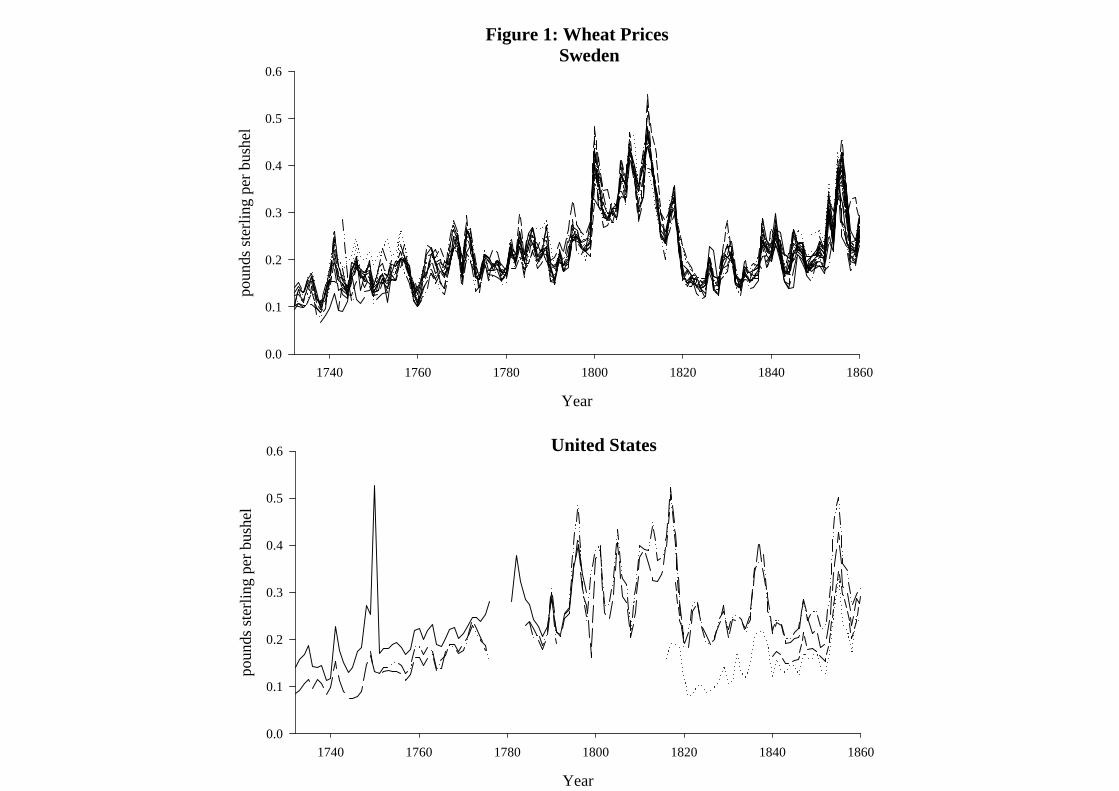
Figure 1: Wheat Prices Sweden

Year

1740 1760 1780 1800 1820 1840 1860

poun

ds st

erlin

g pe

r bus

hel

0.0

0.1

0.2

0.3

0.4

0.5

0.6

United States

Year

1740 1760 1780 1800 1820 1840 1860

poun

ds st

erlin

g pe

r bus

hel

0.0

0.1

0.2

0.3

0.4

0.5

0.6

Figure 2: Beef Prices Sweden

Year

1740 1760 1780 1800 1820 1840 1860

poun

ds st

erlin

g pe

r bbl

0

1

2

3

4

5

6

United States

Year

1740 1760 1780 1800 1820 1840 1860

poun

ds st

erlin

g pe

r bbl

0

1

2

3

4

5

6

4. Price Dispersion

qijk,t = log(Pi ,j ,t)− log(Pi ,k,t)

Figure 3 shows densities for the US, Sweden, and trans-oceanicqijk,t .

Observations: UU: 4,093; SS: 179,156; SU: 43,531.

4. Price Dispersion

qijk,t = log(Pi ,j ,t)− log(Pi ,k,t)

Figure 3 shows densities for the US, Sweden, and trans-oceanicqijk,t .

Observations: UU: 4,093; SS: 179,156; SU: 43,531.

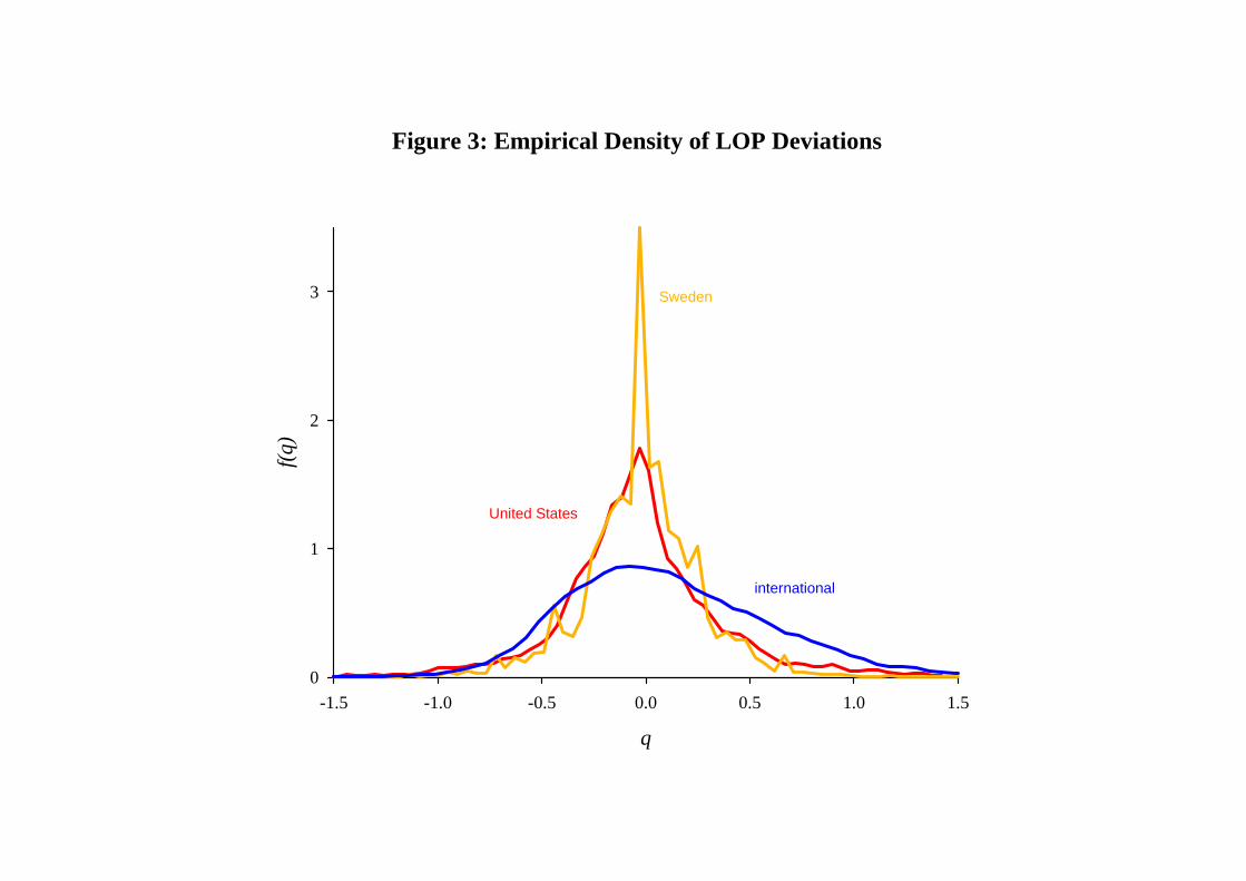
Figure 3: Empirical Density of LOP Deviations

q

-1.5 -1.0 -0.5 0.0 0.5 1.0 1.5

f(q)

0

1

2

3 Sweden

United States

international

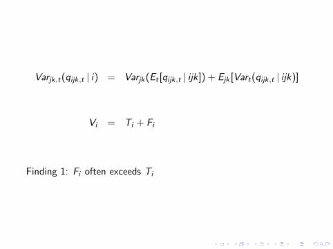
Varjk,t(qijk,t | i) = Varjk(Et [qijk,t | ijk]) + Ejk [Vart(qijk,t | ijk)]

Vi = Ti + Fi

Finding 1: Fi often exceeds Ti

5. HWWTO?

mdaijk = median|qijkt |.

Next, we adopt notation for the time-series mean of each logrelative price:

qijk =T∑

t=1

1

Tqijk,t .

Then the second measure of dispersion is the time-series variance:

Vart(qijk,t) = υijk =T∑

t=1

1

T − 1(qijkt − qijk)2

5. HWWTO?

mdaijk = median|qijkt |.

Next, we adopt notation for the time-series mean of each logrelative price:

qijk =T∑

t=1

1

Tqijk,t .

Then the second measure of dispersion is the time-series variance:

Vart(qijk,t) = υijk =T∑

t=1

1

T − 1(qijkt − qijk)2

The Engel-Rogers (1996) approach:

υijk = αi + βd ln(distance)jk + βodojk + εijk ,

and similarly for mdaijk

Finding 2: Distance is economically and statistically significant, forindividual commodities or in the pool.

Finding 3: The ocean width is insignificant or small.

The border effect is:

exp

(βo

βd

)

For υijk this is 672,000 km with a standard error of 1,216,000 km.

For mdaijk it is 1,350 km with a standard error of 430 km.

But recall the Gorodnichenko-Tesar (2009) critique:

υijk = αi + βd ln(distance)jk + βodojk + βsdsjk + εijk

Finding 4: Measuring ocean-width relative to Swedish pricedispersion does not affect the conclusions.

Figure 3: Empirical Density of LOP Deviations

q

-1.5 -1.0 -0.5 0.0 0.5 1.0 1.5

f(q)

0

1

2

3 Sweden

United States

international

6. What Next I

υijk = αi + βd ln(distance)jk + βodojk + εijk

But:

(a) exp(βo/βd) can be significant even when βo is not, and viceversa(so see Parsley and Wei)

(b) the ocean effect is measured relative to the assumed log-lineardistance effect

6. What Next I

υijk = αi + βd ln(distance)jk + βodojk + εijk

But:

(a) exp(βo/βd) can be significant even when βo is not, and viceversa(so see Parsley and Wei)

(b) the ocean effect is measured relative to the assumed log-lineardistance effect

Figure 4: Volatility and Distance

log distance (thousands of km)

-4 -2 0 2

v(ijk

)

0

20

40

60

intra-United States

intra-Sweden

international

υijk = αi + βd(distancejk + βodojk)1−γi

1− γi+ εijk

6. What Next II

Given the role for Fi and the economic-historical work onconvergence we’ll next study time-varying covariates and timeitself.

6. What Next II

Given the role for Fi and the economic-historical work onconvergence we’ll next study time-varying covariates and timeitself.