Embed Size (px)
Citation preview

How to Compress Interactive Communication
Boaz Barak∗ Mark Braverman† Xi Chen‡ Anup Rao§
October 15, 2010
Abstract
We describe new ways to simulate 2-party communication protocols to get protocols withpotentially smaller communication. We show that every communication protocol that communi-cates C bits and reveals I bits of information about the inputs to the participating parties can besimulated by a new protocol involving at most O(
√CI) bits of communication. If the protocol
reveals I bits of information about the inputs to an observer that watches the communicationin the protocol, we show how to carry out the simulation with O(I) bits of communication.
These results lead to a direct sum theorem for randomized communication complexity. Ig-noring polylogarithmic factors, we show that for worst case computation, computing n copiesof a function requires
√n times the communication required for computing one copy of the
function. For average case complexity, given any distribution µ on inputs, computing n copiesof the function on n inputs sampled independently according to µ requires
√n times the com-
munication for computing one copy. If µ is a product distribution, computing n copies on nindependent inputs sampled according to µ requires n times the communication required forcomputing the function. We also study the complexity of computing the sum (or parity) of nevaluations of f , and obtain results analogous to those above.
As far as we know, our results give the first compression schemes for general randomizedprotocols and the first direct sum results in the general setting. Previous results applied onlywhen the protocols were restricted to running in a bounded number of rounds, where eachmessage can be compressed in turn, and only applied when the parties are given independentinputs.
∗Department of Computer Science, Princeton University, [email protected]. Supported by NSF grantsCNS-0627526, CCF-0426582 and CCF-0832797, US-Israel BSF grant 2004288 and Packard and Sloan fellowships.
†Microsoft Research New England, [email protected].‡Department of Computer Science, Princeton University, [email protected]. Supported by NSF Grants CCF-
0832797 and DMS-0635607.§Center for Computational Intractability, Princeton University, [email protected]. Supported by NSF
Grant CCF 0832797.
1
Contents
1 Introduction 21.0.1 Compressing Communication Protocols . . . . . . . . . . . . . . . . . . . . . 51.0.2 Direct sum theorems . . . . . . . . . . . . . . . . . . . . . . . . . . . . . . . . 51.0.3 XOR Lemmas for communication complexity . . . . . . . . . . . . . . . . . . 6
2 Our Techniques 72.1 Compression According to the Internal Information Cost . . . . . . . . . . . . . . . . 82.2 Compression According to the External Information Cost . . . . . . . . . . . . . . . 9
3 Preliminaries 103.1 Information Theory . . . . . . . . . . . . . . . . . . . . . . . . . . . . . . . . . . . . 103.2 Communication Complexity . . . . . . . . . . . . . . . . . . . . . . . . . . . . . . . . 113.3 Finding differences in inputs . . . . . . . . . . . . . . . . . . . . . . . . . . . . . . . . 123.4 Measures of Information Complexity . . . . . . . . . . . . . . . . . . . . . . . . . . . 12
4 Proof of the direct sum theorems 13
5 Reduction to Small Internal Information Cost 15
6 Compression According to the Internal Information Cost 176.1 A proof sketch . . . . . . . . . . . . . . . . . . . . . . . . . . . . . . . . . . . . . . . 176.2 The actual proof . . . . . . . . . . . . . . . . . . . . . . . . . . . . . . . . . . . . . . 18
7 Compression According to the External Information Cost 217.1 A proof sketch . . . . . . . . . . . . . . . . . . . . . . . . . . . . . . . . . . . . . . . 217.2 The actual proof. . . . . . . . . . . . . . . . . . . . . . . . . . . . . . . . . . . . . . . 227.3 Proof of Theorem 7.5 . . . . . . . . . . . . . . . . . . . . . . . . . . . . . . . . . . . . 25
7.3.1 A single round . . . . . . . . . . . . . . . . . . . . . . . . . . . . . . . . . . . 267.3.2 The whole protocol . . . . . . . . . . . . . . . . . . . . . . . . . . . . . . . . . 29
8 Open problems and final thoughts 30
A A simple generalization of Azuma’s inequality 32
B Analyzing Rejection Sampling 33
C Finding The First Difference in Inputs 34
1
1 Introduction
In this work, we address two questions: (1) Can we compress the communication of an interactiveprotocol so it is close to the information conveyed between the parties? (2) Is it harder to computea function on n independent inputs than to compute it on a single input? In the context ofcommunication complexity, the two questions are related, and our answer to the former will yieldan answer to the latter.
Techniques for message compression, first considered by Shannon [Sha48], have had a big impacton computer science, especially with the rise of the Internet and data intensive applications. Todaywe know how to encode messages so that their length is essentially the same as the amount ofinformation that they carry (see for example the text [CT91]). Can we get a similar savings in aninteractive setting? A first attempt might be to simply compress each message of the interaction inturn. However, this compression involves at least 1 bit of communication for every message of theinteraction, which can be much larger than the total information conveyed between the parties. Inthis paper, we show how compress interactive communication protocols in a way that is independentof the number of rounds of communication, and in some settings, give compressed protocols withcommunication that has an almost linear dependence on the information conveyed in the originalprotocol.
The second question is one of the most basic questions of theoretical computer science, calledthe direct sum question, and is closely related to the direct product question. A direct producttheorem in a particular computational model asserts that the probability of success of performingn independent computational task decreases in n. Famous examples of such theorems includeYao’s XOR Lemma [Yao82] and Raz’s Parallel Repetition Theorem [Raz95]. In the context ofcommunication complexity, Shaltiel [Sha03] gave a direct product theorem for the discrepancy of afunction, but it remains open to give such a theorem for the success probability of communicationtasks. A direct sum theorem asserts that the amount of resources needed to perform n independenttasks grows with n. While the direct sum question for general models such as Boolean circuits hasa long history (cf [Uhl74, Pau76, GF81]), no general results are known, and indeed they cannot beachieved by the standard reductions used in complexity theory, as a black-box reduction mappinga circuit C performing n tasks into a circuit C ′ performing a single task will necessarily makeC ′ larger than C, rather than making it smaller. Indeed it is known that at least the moststraightforward/optimistic formulation of a direct sum theorem for Boolean circuits is false.1
Nevertheless, direct sum theorems are known to hold in other computational models. Forexample, an optimal direct sum theorem is easy to prove for decision tree depth. A more interestingmodel is communication complexity, where this question was first raised by Karchmer, Raz, andWigderson [KRW91] who conjectured a certain direct sum result for deterministic communicationcomplexity of relations, and showed that it would imply that P * NC1. Feder, Kushilevitz, Naor,and Nisan [FKNN91] gave a direct sum theorem for non-deterministic communication complexity,and deduced from it a somewhat weaker result for deterministic communication complexity— if asingle copy of a function f requires C bits of communications, then n copies require Ω(
√Cn) bits.
Feder et al also considered the direct sum question for randomized communication complexity (seealso Open Problem 4.6 in [KN97]) and showed that the dependence of the communication on the
1The example comes from fast matrix multiplication. By a counting argument, there exists an n×n matrix A overGF(2) such that the map x 7→ Ax requires a circuit of Ω(n2/ log n) size. But the map (x1, . . . , xn) 7→ (Ax1, . . . , Axn)is just the product of the matrices A and X (whose columns are x1, . . . , xn) and hence can be carried out by a circuitof O(n2.38) ≪ n · (n2/ log n). See Shaltiel’s paper [Sha03] for more on this question.
2
error of the protocol for many copies can be better than that obtained by the naive protocol formany copies.
Chakrabarti et al [CSWY01] gave a direct sum theorem in the case that the communicationinvolves one simultaneous round of communication, while Jain et al [JRS03] (improved upon by[HJMR07]) gave a direct sum theorem for the distributional complexity of bounded round random-ized protocols when the inputs are assumed to be independent of each other. These results onlyapply when the number of rounds in the protocol is bounded to be less than the total communica-tion, and so give no guarantees in the standard model, with unbounded number of rounds.
All of the works mentioned above, had a common outline that we follow in this work as well.They began by measuring the information that an observer learns about the inputs of the partiesby watching the messages and public randomness of the protocol, a quantity that they called theinformation cost of the protocol. In our paper, we shall refer to this measure of information as theexternal information cost of the protocol, to contrast it with the internal information cost that weshall define later:
Definition 1.1 (External Information Cost). Given a distribution µ on inputs X,Y , and protocolπ, denoting by π(X,Y ) the public randomness and messages exchanged during the protocol, theexternal information cost ICo
µ(π) is defined to be the mutual information between the inputs andπ(X,Y ):
ICoµ(π)
def= I(XY ;π(X,Y ))
The external information cost is always smaller than the communication complexity, and ifthe inputs to the parties are independent of each other (i.e. X is independent of Y ), an optimaldirect sum theorem can be proved for this measure of complexity. This means that from a protocolcomputing n copies of f with communication C, one can obtain a protocol computing f withexternal information cost C/n, as long as the inputs to f are independent of each other. Thus theproblem of proving direct sum theorems for independent inputs reduces to the problem of simulatinga protocol τ with small external information cost with a protocol ρ that has small communication.That is, the direct sum question reduces to the problem of protocol compression. Previous workscarried out the compression by compressing every message of the protocol individually, hence thedependency on the number of rounds. Our stronger method of compression allows us to get newdirect sum theorems that are independent of the number of rounds of communication.
In our work we work with two different measures of the information complexity of a commu-nication protocol. The first is the external information cost, defined above. The second measure,which we call the internal information cost of the protocol, is the information that the parties inthe protocol learn by watching the messages and public randomness of the protocol, that they didnot already know. Formally,
Definition 1.2 (Internal Information Cost). Given a distribution µ on inputs X,Y , and protocolπ, denoting by π(X,Y ) the public randomness and messages exchanged during the protocol, theinternal information cost ICi
µ(π) is defined to be
ICiµ(π)
def= I(X;π(X,Y )|Y ) + I(Y ;π(X,Y )|X).
Since each party knows her own input, the protocol can only reveal less information to herthan to an independent observer. Indeed, it can be shown that the internal information cost isnever larger than the external information cost and that the two are equal if the inputs X,Y
3
are independent of each other. However, in the case that the inputs are dependent, the internalinformation cost may be significantly smaller — for example, if µ is a distribution where X = Yalways, then the internal information cost is always 0, though the external information cost maybe arbitrarily large. It is also easy to check that if π is deterministic, then the internal informationcost is simply the sum of the entropies ICi
µ(π) = H(π(X,Y )|Y )+H(π(X,Y )|X), which is the sameas H(π(X,Y )) if X,Y are independent.
The notion of internal information cost was used implicitly by Bar-Yossef et al [BYJKS04], anda direct sum theorem for this notion (using the techniques originating from Razborov [Raz92] andRaz [Raz95]) is implicit in their work. This direct sum theorem holds whether or not the inputsto the parties are independent of each other, unlike the analogous result for external informationcost. We can convert any protocol computing n copies of f with communication C into one thatcomputes f with internal information cost C/n and communication complexity C.
Our most important contributions are two new protocol compression methods that reduce thecommunication of protocols in terms of their information costs. Indeed, the work of [JRS03,HJMR07] can be viewed as giving ways to compress one round protocols with small externalinformation. In this setting, the external information of a protocol is simply I(X;M), where Mis the single message in the protocol and X is the input used to generate the message. [JRS03,HJMR07] showed how to simulate the sending of such a message using I(X;M)+
√
I(X;M)+O(1)bits. Related problems have also been considered in the information theory literature. Stated in ourlanguage, the now classical Slepian-Wolf theorem [SW73] (see also [WZ76]) is about compressingone round deterministic protocols according to the internal information cost of the protocol. Inthis case, the internal information cost is simply I(X;M |Y ) = H(M |Y ), where here X,Y arethe inputs and M is the lone message transmitted by the first party. The theorem shows how totransmit n independent M1, . . . ,Mn to a receiver that knows the corresponding Y1, . . . , Yn, usingamortized (one way) communication that is close to the internal information cost. In contrast,the results in our work are about compressing a single interaction, which is a harder problem,since one may always repeat the result of the compression n times. A caveat is that the results ofrunning our compression schemes give interactive communication protocols, as opposed to one waycommunication protocols.
We give two methods to compress protocols. Our first method shows that one can always sim-ulate a protocol of internal information cost I and communication complexity C using an expectednumber of O(
√IC) communication bits. The second method shows how to simulate a protocol of
external information cost I with O(I) communication. Note that in both cases the communicationcomplexity of the simulation is independent of the number of rounds. Indeed, these are the firstcompression schemes that do true protocol compression, as opposed to compressing each round ata time, and are the first results that succeed for randomized protocols even when the inputs arenot independent.
As a result, we obtain the first non-trivial direct sum theorem for randomized communicationcomplexity. Loosely speaking, letting fn be the function that outputs the concatenation of ninvocations of f on independent inputs, and letting f+n be the function that outputs the XOR of nsuch invocations, we show that (a) the randomized communication complexity of both fn and f+n
is up to logarithmic factors√n times the communication complexity of f , and (b) the distributional
complexity of both fn and f+n over the distribution µn, where µ is a product distribution overindividual input pairs, is n times the distributional complexity of f .2
2In both (a) and (b), there is a loss of a constant additive factor in the actual statement of the result for f+n.
4

1.0.1 Compressing Communication Protocols
We give two new protocol compression algorithms, that take a protocol π whose information costis small and transform it into a protocol τ of small communication complexity.3 Below we denotethe communication complexity of a protocol τ by CC(τ).
Theorem 1.3. For every distribution µ, every protocol π, and every ǫ > 0, there exists func-
tions πx, πy, and a protocol τ such that |πx(X, τ(X,Y )) − π(X,Y )| < ǫ, Pr[πx(X, τ(X,Y )) 6=πy(Y, τ(X,Y ))] < ǫ and
CC(τ) ≤ O
(
√
CC(π) · ICiµ(π)
log(CC(π)/ǫ)
ǫ
)
.
If the players want to obtain the results of running the protocol π, they can run τ instead andthen use the functions πx, πy to reconstruct the effects of running π. The condition |πx(X, τ(X,Y ))−π(X,Y )| < ǫ ensures that the transcript of τ specifies a unique leaf in the protocol tree for π insuch a way that this leaf is ǫ-close in statistical distance to the leaf sampled by π. The conditionthat Pr[πx(X, τ(X,Y )) 6= πy(Y, τ(X,Y ))] < ǫ guarantees that with high probability both playersachieve a consensus on what the sampled leaf was. Thus, the triple τ, πx, πy specify a new protocolthat is a compression of π.
Our second result gives a simulation for protocols with small external information cost:
Theorem 1.4. For every distribution µ, every protocol π, and every α > 0, there exists func-
tions πx, πy, and a protocol τ such that |πx(X, τ(X,Y )) − π(X,Y )| < α, Pr[πx(X, τ(X,Y )) 6=πy(Y, τ(X,Y ))] < α and
CC(τ) ≤ O
(
ICoµ(π)
log(CC(π)/α)
α2
)
.
Our results can be viewed as a generalization of the traditional notion of string compression,a notion that applies only to the restricted case of deterministic one way protocols. In the abovetheorems, our compressed protocols may use public randomness that can be large (though stillbounded in terms of the communication complexity of the original protocol). However, we notethat by the results of Newman [New91], any protocol that achieves some functionality can beconverted into another protocol that achieves the same functionality and uses few public randombits. Thus our compression schemes are useful even when public randomness is expensive.
1.0.2 Direct sum theorems
Given a function f : X ×Y → Z, we define the function fn : X n×Yn → Zn to be the concatenationof the evaluations:
fn(x1, . . . , xn, y1, . . . , yn)def= (f(x1, y1), f(x2, y2), . . . , f(xn, yn)).
Denote by Rρ(f) the communication complexity of the best randomized public coin protocolfor computing f that errs with probability at most ρ. In this paper we show:
This accounts for the fact that if, say, f is the XOR function itself then clearly there is no direct sum theorem. SeeRemark 1.12.
3 We note that this is in the communication complexity model, and hence these algorithms are not necessarilycomputationally efficient. Even for single message compression, there are distributions with small entropy that cannotbe efficiently compressed (e.g. pseudorandom distributions).
5

Theorem 1.5 (Direct Sum for Randomized Communication Complexity). For every α > 0,
Rρ(fn) · log (Rρ(f
n)/α) ≥ Ω(
Rρ+α(f)α√n)
Theorem 1.5 is obtained using Yao’s min-max principle from an analogous theorem for distri-
butional communication complexity. For a distribution µ on the inputs X × Y, we write Dµρ (f) to
denote the communication complexity of the best protocol (randomized or deterministic) that com-putes f with probability of error at most ρ when the inputs are sampled according to µ. We writeµn to denote the distribution on n inputs, where each is sampled according to µ independently.
We first state the direct sum theorem for information content that is implicit in the work of[BYJKS04].
Theorem 1.6. For every µ, f, ρ there exists a protocol τ computing f on inputs drawn from µ with
probability of error at most ρ and communication at most Dµn
ρ (fn) such that ICiµ(τ) ≤ 2Dµn
ρ (fn)n .
Compressing protocol τ above using Theorem 1.3 reduces the communication of this protocol
to O
(
√
ICiµ(τ)D
µn
ρ (fn)
)
= O(Dµn
ρ (fn)√n). Formally, we prove:
Theorem 1.7 (Direct Sum for Distributional Communication Complexity). For every α > 0,
Dµn
ρ (fn) · log(
Dµn
ρ (fn)/α)
≥ Ω(
Dµρ+α(f)α
√n)
The communication complexity bound of Theorem 1.7 only grows as the square root of thenumber of repetitions. However, in the case that the distribution on inputs is a product distribution,we use our stronger compression (Theorem 1.4) to obtain a direct sum theorem that is optimal upto logarithmic factor:
Theorem 1.8 (Direct Sum for Product Distributions). If µ is a product distribution, then for
every α > 0Dµn
ρ (fn) · polylog(
Dµn
ρ (fn)/α)
≥ Ω(
Dµρ+α(f)α
2n)
1.0.3 XOR Lemmas for communication complexity
When n is very large in terms of the other quantities, the above theorems can be superseded bytrivial arguments, since fn must require at least n bits of communication just to describe theoutput. Our next set of theorems show that almost the same bounds apply to the complexity ofthe XOR (or more generally sum modulo K) of n copies of f , where the trivial arguments do nothold. Assume that the output of the function f is in the group ZK for some integer K, and define
f+n(x1, . . . , xn, y1, . . . , yn)def=
n∑
i=1
f(xi, yi).
We have the following results for the complexity of f+n:
Theorem 1.9 (XOR Lemma for Randomized Communication Complexity). For every α > 0,
Rρ(f+n) · log
(
Rρ(f+n)/α
)
≥ Ω(
(Rρ+α(f)− 2 logK)α√n)
6
Theorem 1.10 (XOR Lemma for Distributional Communication Complexity). For every α > 0,
Dµn
ρ (f+n) · log(
Dµn
ρ (f+n)/α)
≥ Ω((
Dµρ+α(f)− 2 logK
)
α√n)
Theorem 1.11 (XOR Lemma for Product Distributions). If µ is a product distribution, then for
every α > 0,Dµn
ρ (f+n) · polylog(
Dµn
ρ (f+n)/α)
≥ Ω((
Dµρ+α(f)− 2 logK
)
αn)
Remark 1.12. If f : ZK×ZK → ZK is itself the sum function, then the communication complexityof f+n does not grow at all, since there is a simple protocol to compute
∑
i(xi+yi) =∑
i xi+∑
j yjusing 2 logK bits. This suggests that some kind of additive loss (like the 2 logK term above) isnecessary in the above theorems.
2 Our Techniques
We now give an informal overview of our compression algorithms. Our direct sum results areobtained in Section 4 by combining these with the direct sum for information content proven inSection 5. Full description of the compression algorithms are given in Section 6 (for the generalcase) and Section 7 (for the product distribution case).
The goal of our compression algorithms is to take a protocol that uses large amounts of com-munication and conveys little information, and convert it into a protocol that makes better useof the communication to achieve better communication complexity. (Such algorithms need not benecessarily computationally efficient, see Footnote 3.)
Note that generic message compression can be fit into this context by considering a deterministicone-way protocol, where player X needs to send a message to player Y . In this classical setting it iswell known that protocol compression (i.e. simple data compression) can be achieved. In principle,one could try to apply round-by-round message compression to compress entire protocols. Thisapproach suffers from the following fatal flaw: individual messages may (and are even likely) tocontain ≪ 1 bits of information. The communication cost of ≥ 1 bit per round would thus be ≫information content of the round. Thus any attempt to implement the compression on a round-by-round basis, as opposed to an entire-protocol basis may work when the number of rounds isbounded, but is doomed to fail in general.
An instructive example on conveying a subconstant amount of information that we will use laterin this exposition is the following. Suppose that player X gets n independent random bits x1, . . . , xnand Y has no information about them. X then computes the majority m = MAJ(x1, . . . , xn) andsends it to Y . With a perfectly random prior, the bit m is perfectly balanced, and thus in totalX conveys one bit of information to Y . Suppose that in the protocol Y only really cared aboutthe value of x5. How much information did X convey about the input x5? By symmetry andindependence of the inputs, X conveys 1/n bits of information about x5. After the bit m (supposem = 1) is received by Y , her estimate of P [x5 = 1] changes from 1/2 to 1/2 + Θ(1/
√n). The fact
that changing the probability from 1/2 to 1/2 + ǫ only costs ǫ2 bits of information is the cause forthe suboptimality of our general compression algorithm.
There are several challenges that need to be overcome to compress an arbitrary protocol. Aninteresting case to consider is a protocol where the players alternate sending each other messages,and each transmitted message is just a bit with information content ǫ ≪ 1. In this case, we cannotafford to even transmit one bit to simulate each of the messages, since that would incur an overhead
7
of 1/ǫ, which would be too large for our application. This barrier was one of the big stumblingblocks for earlier works, which is why their results applied only when the number of rounds in theprotocols was forced to be small.
We give two simulation protocols to solve this problem. The first solution works for all distribu-tions, achieving sub-optimal parameters, while the second works only for product input distributionsand achieves optimal parameters up to poly-logarithmic factors. In both solutions, the players sim-ulate the original protocol π using shared randomness. The intuition is that if a message containsa small amount of information, then we do not need to communicate it, and can sample it usingshared randomness instead.
v
u
0 1 0 0 1 1 1 0
O v , x ( 0 ) [ O v , y ( 0 ) ] O v , x ( 1 ) [ O v , y ( 1 ) ]
O u , y ( 0 ) [ O u , x ( 0 ) ] O u , y ( 1 ) [ O u , x ( 1 ) ]
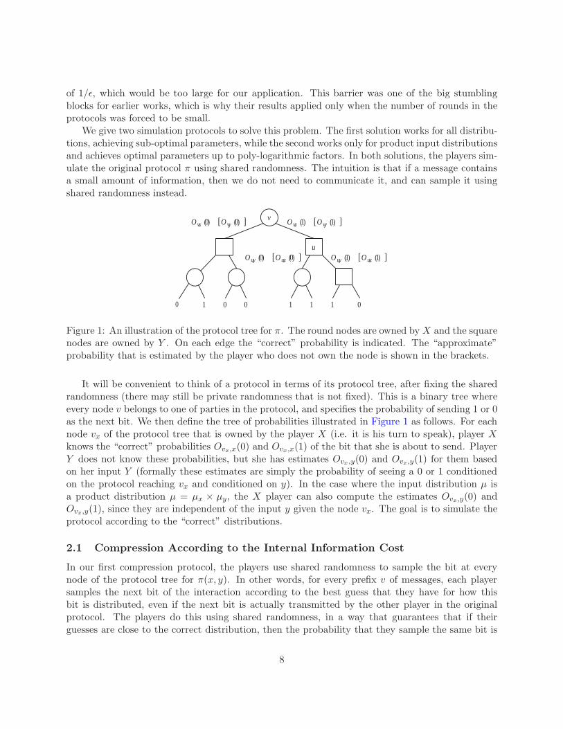
Figure 1: An illustration of the protocol tree for π. The round nodes are owned by X and the squarenodes are owned by Y . On each edge the “correct” probability is indicated. The “approximate”probability that is estimated by the player who does not own the node is shown in the brackets.
It will be convenient to think of a protocol in terms of its protocol tree, after fixing the sharedrandomness (there may still be private randomness that is not fixed). This is a binary tree whereevery node v belongs to one of parties in the protocol, and specifies the probability of sending 1 or 0as the next bit. We then define the tree of probabilities illustrated in Figure 1 as follows. For eachnode vx of the protocol tree that is owned by the player X (i.e. it is his turn to speak), player Xknows the “correct” probabilities Ovx,x(0) and Ovx,x(1) of the bit that she is about to send. PlayerY does not know these probabilities, but she has estimates Ovx,y(0) and Ovx,y(1) for them basedon her input Y (formally these estimates are simply the probability of seeing a 0 or 1 conditionedon the protocol reaching vx and conditioned on y). In the case where the input distribution µ isa product distribution µ = µx × µy, the X player can also compute the estimates Ovx,y(0) andOvx,y(1), since they are independent of the input y given the node vx. The goal is to simulate theprotocol according to the “correct” distributions.
2.1 Compression According to the Internal Information Cost
In our first compression protocol, the players use shared randomness to sample the bit at everynode of the protocol tree for π(x, y). In other words, for every prefix v of messages, each playersamples the next bit of the interaction according to the best guess that they have for how thisbit is distributed, even if the next bit is actually transmitted by the other player in the originalprotocol. The players do this using shared randomness, in a way that guarantees that if theirguesses are close to the correct distribution, then the probability that they sample the same bit is
8
high. More precisely, the players share a random number κv ∈ [0, 1] for every node v in the tree,and each player guesses the next bit following v to be 1, if the player’s estimated probability forthe message being 1 is at least κv. Note that the player that owns v samples the next bit withthe correct probability. It is not hard to see that the probability of getting inconsistent samples
at the node v is at most |Ov,x − Ov,y|def= |Ov,x(0) − Ov,y(0)| + |Ov,x(1) − Ov,y(1)|. Once they
have each sampled from the possible interactions, we shall argue that there is a correct leaf in theprotocol tree, whose distribution is exactly the same as the leaf in the original protocol. This isthe leaf that is obtained by starting at the root and repeatedly taking the edge that was sampledby the owner of the node. We then show how the players can use hashing and binary search tocommunicate a polylogarithmic number of bits with each other to resolve the inconsistencies intheir samples and find this correct path with high probability. In this way, the final outcome willbe statistically close to the distribution of the original protocol. An example run for this protocolis illustrated in Figure 2. The additional interaction cost scales according to the expected numberof inconsistencies on the path to the correct leaf, which we show can be bounded by
√I · C, where
I is the information content and C is the communication cost of the original protocol.Recall from the Majority example above that ǫ information can mean that |Ov,x −Ov,y | ≈
√ǫ.
In fact, the “worst case” example for us is when in each round I/C information is conveyed, leadingto a per-round error of
√
I/C and a total expected number of mistakes of√
I/C · C =√I · C.
2.2 Compression According to the External Information Cost
Our more efficient solution gives a protocol with communication complexity within polylogarithmicfactors of the external information cost. It is illustrated on Figure 3. The idea in this case isto simulate chunks of the protocol that convey a constant amount of information each. If wecan simulate a portion of the protocol that conveys a constant (or even 1/poly-log) amount ofinformation using poly-logarithmic number of bits of communication, then we can simulate theentire protocol using O(I) bits of communication.
The advantage the players have in the case that we are measuring information from the view-point of an observer is that for each node in the tree, the player who owns that node knows not onlythe correct distribution for the next bit, but also knows what the distribution that the observer hasin mind is. They can use this shared knowledge to sample entire paths according to the distributionthat is common knowledge at every step. In general, the distribution of the sampled path can de-viate quite a bit from the correct distribution. However, we argue that if the information conveyedon a path is small (1/polylog bit), then the difference between the correct and the approximateprobability is constant. After sampling the approximate bits for the appropriate number of steps soas to cover 1/polylog information, the players can communicate to estimate the correct probabilitywith which this node was supposed to occur. The players can then either accept the sequence orresample a new sequence in order to get a final sample that behaves in a way that is close to thedistribution of the original protocol.
There are several technical challenges involved in getting this to work. The fact that the inputsof the players are independent is important for the players to decide how many messages the playersshould try to sample at once to get to the frontier where 1/polylog bits of information have beenrevealed. When the players’ inputs are dependent, they cannot estimate how many messages theyshould sample before the information content becomes too high, and we are unable to make thisapproach work.
9
3 Preliminaries
Notation. We reserve capital letters for random variables and distributions, calligraphic lettersfor sets, and small letters for elements of sets. Throughout this paper, we often use the notation |bto denote conditioning on the event B = b. Thus A|b is shorthand for A|B = b. Given a sequenceof symbols A = A1, A2, . . . , Ak, we use A≤j denote the prefix of length j.
We use the standard notion of statistical/total variation distance between two distributions.
Definition 3.1. Let D and F be two random variables taking values in a set S. Their statisticaldistance is
|D − F | def= maxT ⊆S
(|Pr[D ∈ T ]− Pr[F ∈ T ]|) = 1
2
∑
s∈S|Pr[D = s]− Pr[F = s]|
If |D − F | ≤ ǫ we shall say that D is ǫ-close to F . We shall also use the notation Dǫ≈ F to mean
D is ǫ-close to F .
3.1 Information Theory
Definition 3.2 (Entropy). The entropy of a random variableX isH(X)def=∑
x Pr[X = x] log(1/Pr[X =x]). The conditional entropy H(X|Y ) is defined to be Ey∈
RY [H(X|Y = y)].
Fact 3.3. H(AB) = H(A) +H(B|A).
Definition 3.4 (Mutual Information). The mutual information between two random variablesA,B, denoted I(A;B) is defined to be the quantity H(A) − H(A|B) = H(B) − H(B|A). Theconditional mutual information I(A;B|C) is H(A|C)−H(A|BC).
In analogy with the fact that H(AB) = H(A) +H(B|A),
Proposition 3.5. Let C1, C2,D,B be random variables. Then
I(C1C2;B|D) = I(C1;B|D) + I(C2;B|C1D).
The previous proposition immediately implies the following:
Proposition 3.6 (Super-Additivity of Mutual Information). Let C1, C2,D,B be random variables
such that for every fixing of D, C1 and C2 are independent. Then
I(C1;B|D) + I(C2;B|D) ≤ I(C1C2;B|D).
We also use the notion of divergence, which is a different way to measure the distance betweentwo distributions:
Definition 3.7 (Divergence). The informational divergence between two distributions is D (A||B)def=
∑
xA(x) log(A(x)/B(x)).
For example, if B is the uniform distribution on 0, 1n then D (A||B) = n−H(A).
Proposition 3.8. D (A||B) ≥ |A−B|2.
10
Proposition 3.9. Let A,B,C be random variables in the same probability space. For every a in
the support of A and c in the support of C, let Ba denote B|A = a and Bac denote B|A = a,C = c.Then I(A;B|C) = Ea,c∈
RA,C [D (Bac||Bc)]
The above facts imply the following easy proposition:
Proposition 3.10. With notation as in Proposition 3.9, for any random variables A,B,
Ea∈
RA[|(Ba)−B|] ≤
√
I(A;B).
Proof.
Ea∈
RA[|(Ba)−B|] ≤ E
a∈RA
[
√
D (Ba||B)]
≤√
Ea∈
RA[D (Ba||B)] by convexity
=√
I(A;B) by Proposition 3.9
3.2 Communication Complexity
Let X ,Y denote the set of possible inputs to the two players, who we name Px, Py. In this paper4,we view a private coins protocol for computing a function f : X × Y → ZK as a binary tree withthe following structure:
• Each node is owned by Px or by Py
• For every x ∈ X , each internal node v owned by Px is associated with a distribution Ov,x
supported on the children of v. Similarly, for every y ∈ Y, each internal node v owned by Py
is associated with a distribution Ov,y supported on the children of v.
• The leaves of the protocol are labeled by output values from ZK .
On input x, y, the protocol π is executed as in Figure 4.A public coin protocol is a distribution on private coins protocols, run by first using shared
randomness to sample an index r and then running the corresponding private coin protocol πr.Every private coin protocol is thus a public coin protocol. The protocol is called deterministic ifall distributions labeling the nodes have support size 1.
Definition 3.11. The communication complexity of a public coin protocol π, denoted CC(π), isthe maximum depth of the protocol trees in the support of π.
Given a protocol π, π(x, y) denotes the concatenation of the public randomness with all themessages that are sent during the execution of π. We call this the transcript of the protocol. Weshall use the notation π(x, y)j to refer to the j’th transmitted bit in the protocol. We write π(x, y)≤j
to denote the concatenation of the public randomness in the protocol with the first j message bits
4The definitions we present here are equivalent to the classical definitions and are more convenient for our proofs.
11
that were transmitted in the protocol. Given a transcript, or a prefix of the transcript, v, we writeCC(v) to denote the number of message bits in v (i.e. the length of the communication).
We often assume that every leaf in the protocol is at the same depth. We can do this since ifsome leaf is at depth less than the maximum, we can modify the protocol by adding dummy nodeswhich are always picked with probability 1, until all leaves are at the same depth. This does notchange the communication complexity.
Definition 3.12 (Communication Complexity notation). For a function f : X × Y → ZK , adistribution µ supported on X × Y, and a parameter ρ > 0, Dµ
ρ (f) denotes the communicationcomplexity of the cheapest deterministic protocol for computing f on inputs sampled according toµ with error ρ. Rρ(f) denotes the cost of the best randomized public coin protocol for computingf with error at most ρ on every input.
We shall use the following fact, first observed by Yao:
Fact 3.13 (Yao’s Min-Max). Rρ(f) = maxµDµρ (f).
3.3 Finding differences in inputs
We use the following lemma of Feige et al. [FPRU94]:
Lemma 3.14 ([FPRU94]). There is a randomized public coin protocol τ with communication com-
plexity O(log(k/ǫ)) such that on input two k-bit strings x, y, it outputs the first index i ∈ [k] suchthat xi 6= yi with probability at least 1− ǫ, if such an i exists.
For completeness, we include the proof (based on hashing) in Appendix C.
3.4 Measures of Information Complexity
Here we briefly discuss the two measures of information cost defined in the introduction.Let R be the public randomness, and X,Y be the inputs to the protocol π. By the chain rule
for mutual information,
ICoµ(π) = I(XY ;π(X,Y ))
= I(XY ;R) +
CC(π)∑
i=1
I(XY ;π(X,Y )i|π(X,Y )<i)
= 0 +
CC(π)∑
i=1
I(XY ;π(X,Y )i|π(X,Y )<i)
ICiµ(π) = I(X;π(X,Y )|Y ) + I(Y ;π(X,Y ))
= I(X;R|Y ) + I(Y ;R|X) +
CC(π)∑
i=1
I(X;π(X,Y )i|Y π(X,Y )<i) + I(Y ;π(X,Y )i|Xπ(X,Y )<i)
= 0 +
CC(π)∑
i=1
I(X;π(X,Y )i|Y π(X,Y )<i) + I(Y ;π(X,Y )i|Xπ(X,Y )<i)
12
Let w be any fixed prefix of the transcript of length i− 1. If it is the X player’s turn to speakin the protocol, I(Y ;π(X,Y )i|X,π(X,Y )≤i−1 = w) = 0. If it is the Y player’s turn to speak, thenI(X;π(X,Y )i|Y, π(X,Y )≤i−1 = w) = 0. On the other hand I(XY ;π(X,Y )i|π(X,Y )≤i−1 = w) ≥maxI(X;π(X,Y )i|Y π(X,Y )≤i−1 = w), I(Y ;π(X,Y )i|Xπ(X,Y )≤i−1 = w) by the chain rule.
Thus, we get that
Fact 3.15. ICoµ(π) ≥ ICi
mu(π).
If µ is a product distribution,
I(XY ;π(X,Y )i|π(X,Y )≤i−1 = w)
= I(X;π(X,Y )i|π(X,Y )≤i−1 = w) + I(Y ;π(X,Y )i|Xπ(X,Y )≤i−1 = w)
= I(X;π(X,Y )i|Y π(X,Y )≤i−1 = w) + I(Y ;π(X,Y )i|Xπ(X,Y )≤i−1 = w)
So we can conclude,
Fact 3.16. If µ is a product distribution, ICiµ(π) = ICo
µ(π).
We note that ICiµ(π) and ICo
µ(π) can be arbitrarily far apart, for example if µ is such thatPr[X = Y ] = 1, then ICi
µ(π) = 0, even though ICoµ(π) may be arbitrarily large.
A remark on the role of public and private randomness Public randomness is consideredpart of the protocol’s transcript. But even if the randomness is short compared to the overallcommunication complexity, making it public can have a dramatic effect on the information contentof the protocol. (As an example, consider a protocol where one party sends a message of x⊕r wherex is its input and r is random. If the randomness r is private then this message has zero informationcontent. If the randomness is public then the message completely reveals the input. This protocolmay seem trivial since its communication complexity is larger than the input length, but in factwe will be dealing with exactly such protocols, as our goal will be to “compress” communication ofprotocols that have very large communication complexity, but very small information content.)
4 Proof of the direct sum theorems
In this section, we prove our direct sum theorems. By Yao’s minimax principle, for every func-tion f , Rρ(f) = maxµD
µρ (f). Thus Theorem 1.7 implies Theorem 1.5 and Theorem 1.10 implies
Theorem 1.9. So we shall focus on proving Theorem 1.7, Theorem 1.8, and the XOR LemmasTheorem 1.10 and Theorem 1.11.
By Theorem 1.6, the main step to establish Theorem 1.7 is to give an efficient simulation of aprotocol with small information content by a protocol with small communication complexity. Weshall use our two results on compression, that we restate here:
Theorem 1.3 (Restated). For every distribution µ, every protocol π, and every ǫ > 0, there exists
functions πx, πy, and a protocol τ such that |πx(X, τ(X,Y )) − π(X,Y )| < ǫ, Pr[πx(X, τ(X,Y )) 6=πy(Y, τ(X,Y ))] < ǫ and
CC(τ) ≤ O
(
√
CC(π) · ICiµ(π)
log(CC(π)/ǫ)
ǫ
)
.
13
Theorem 1.4 (Restated). For every distribution µ, every protocol π, and every α > 0, there exists
functions πx, πy, and a protocol τ such that |πx(X, τ(X,Y )) − π(X,Y )| < α, Pr[πx(X, τ(X,Y )) 6=πy(Y, τ(X,Y ))] < α and
CC(τ) ≤ O
(
ICoµ(π)
log(CC(π)/α)
α2
)
.
Proof of Theorem 1.5 from Theorem 1.3. Let π be any protocol computing fn on inputsdrawn from µn with probability of error less than ρ. Then by Theorem 1.6, there exists a protocolτ1 computing f on inputs drawn from µ with error at most ρ with CC(τ1) ≤ CC(π) and ICi
µ(τ1) ≤2CC(π)/n. Next, applying Theorem 1.3 to the protocol τ1 gives that there must exist a protocol τ2computing f on inputs drawn from µ with error at most ρ+ α and
CC(τ2) ≤ O
(
√
CC(τ1)ICiµ(τ1) log(CC(τ1)/α)/α
)
= O(
√
CC(π)CC(π)/n log(CC(π)/α)/α)
= O
(
CC(π) log(CC(π)/α)/α√n
)
This proves Theorem 1.7.
Proof of Theorem 1.8 from Theorem 1.4. Let π be any protocol computing fn on inputsdrawn from µn with probability of error less than ρ. Then by Theorem 1.6, there exists a protocolτ1 computing f on inputs drawn from µ with error at most ρ with CC(τ1) ≤ CC(π) and ICi
µ(τ1) ≤2CC(π)/n. Since µ is a product distribution, we have that ICo
µ(π) = ICiµ(π). Next, applying
Theorem 1.4 to the protocol τ1 gives that there must exist a protocol τ2 computing f on inputsdrawn from µ with error at most ρ+ α and
CC(τ2) ≤ O(
ICoµ(τ1) log(CC(τ1)/α)/α
2)
= O
(
CC(π) log(CC(π)/α)
nα2
)
This proves Theorem 1.8.
Proof of the XOR Lemma. The proof for Theorem 1.10 (XOR Lemma for distributional com-plexity) is very similar. First, we show an XOR-analog of Theorem 1.6:
Theorem 4.1. For every distribution µ, there exists a protocol τ computing f with probability of
error ρ over the distribution µ with CC(τ) ≤ Dµn
ρ (f+n) + 2 logK such that if τ ′ is the protocol that
is the same as τ but stops running after Dµn
ρ (f+n) message bits have been sent, then ICiµ(τ
′) ≤2Dµn
ρ (fn+)n .
Now let π be any protocol computing f+n on inputs drawn from µn with probability of errorless than ρ. Then by Theorem 4.1, there exists a protocol τ1 computing f on inputs drawn fromµ with error at most ρ with CC(τ1) ≤ CC(π) + 2 logK and such that if τ ′1 denotes the first CC(π)bits of the message part of the transcript, ICi
µ(τ′1) ≤ 2CC(π)/n. Next, applying Theorem 1.3 to
14

the protocol τ ′1 gives that there must exist a protocol τ ′2 simulating τ ′1 on inputs drawn from µ witherror at most ρ+ α and
CC(τ ′2) ≤ O
(
√
CC(τ ′1)ICiµ(τ
′1) log(CC(τ
′1)/α)/α
)
= O(
√
CC(π)CC(π)/n log(CC(π)/α)/α)
= O
(
CC(π) log(CC(π)/α)/α√n
)
Finally we get a protocol for computing f by first running τ ′2 and then running the last 2 logK
bits of π. Thus we must have that O(
CC(π) log(CC(π)/α)/α√n
)
+2 logK ≤ Dµρ+α(f), as in the theorem.
5 Reduction to Small Internal Information Cost
We now prove Theorem 1.6 and Theorem 4.1, showing that the existence of a protocol with com-munication complexity C for fn (or f+n) implies a protocol for f with information content roughlyC/n.
Theorem 1.6 (Restated). For every µ, f, ρ there exists a protocol τ computing f on inputs drawn
from µ with probability of error at most ρ and communication at most Dµn
ρ (fn) such that ICiµ(τ) ≤
2Dµn
ρ (fn)n .
Theorem 4.1 (Restated). For every distribution µ, there exists a protocol τ computing f with
probability of error ρ over the distribution µ with CC(τ) ≤ Dµn
ρ (f+n)+ 2 logK such that if τ ′ is theprotocol that is the same as τ but stops running after D
µn
ρ (f+n) message bits have been sent, then
ICiµ(τ
′) ≤ 2Dµn
ρ (fn+)n .
The key idea involved in proving the above theorems is a way to split dependencies betweenthe inputs that arose in the study of lowerbounds for the communication complexity of disjointnessand in the study of parallel repetition [KS92, Raz92, Raz95].
Proof. Fix µ, f, n, ρ as in the statement of the theorems. We shall prove Theorem 1.6 first.Theorem 4.1 will easily follow by the nature of our proof. To prove Theorem 1.6, we show how touse the best protocol for computing fn to get a protocol with small information content computingf . Let π be a deterministic protocol with communication complexity D
µn
ρ (fn) computing fn withprobability of error at most ρ.
Let (X1, Y1), . . . , (Xn, Yn) denote random variables distributed according to µn. Let π(Xn, Y n)denote the random variable of the transcript (which is just the concatenation of all messages, sincethis is a deterministic protocol) that is obtained by running the protocol π on inputs (X1, Y1), . . . ,(Xn, Yn). We define random variables W = W1, . . . ,Wn where each Wj takes value in the disjointunion X ⊎ Y so that each Wj = Xj with probability 1/2 and Wj = Yj with probability 1/2. LetW−j denote W1, . . . ,Wj−1,Wj+1, . . . ,Wn.
15
Our new protocol τ shall operate as in Figure 5. Note the distinction between public and private
randomness. This distinction make a crucial difference in the definition of information content, asmaking more of the randomness public reduces the information content of a protocol.
The probability that the protocol τ makes an error on inputs sampled from µ is at most theprobability that the protocol π makes an error on inputs sampled from µn. It is also immediatethat CC(τ) = CC(π). All that remains is to bound the information content ICi
µ(τ). We do this byrelating it to the communication complexity of π.
To simplify notation, below we will use π to denote π(X,Y ) when convenient.
Dµn
ρ (fn) ≥ CC(π) ≥ I(X1 · · ·XnY1 · · ·Yn;π|W ) ≥n∑
j=1
I(XjYj ;π|W ) = nI(XJYJ ;π|WJ),
where the last inequality follows from Proposition 3.6. Next observe that the variables JW−J areindependent of XJ , YJ ,WJ . Thus we can write
I(XJYJ ;π|JW ) = I(XJYJ ;π|JWJW−J) + I(XJYJ ;JW
−J |WJ)
= I(XJYJ ;JW−Jπ|WJ)
= I(XY ;JW−Jπ|WJ)
=I(XY ;JW−Jπ|XJ) + I(XY ;JW−Jπ|YJ)
2
=I(Y ;JW−Jπ|XJ ) + I(X;JW−Jπ|YJ)
2,
where the last equality follows from the fact that XJ determines X and YJ determines Y . This lastquantity is simply the information content of τ . Thus we have shown that CC(π) ≥ (n/2)ICi
µ(τ)as required.
Remark 5.1. The analysis above can be easily improved to get the bound ICiµ(τ) ≤ CC(τ)/n by
taking advantage of the fact that each bit of the transcript gives information about at most one ofthe players’ inputs, but for simplicity we do not prove this here.
This completes the proof for Theorem 1.6. The proof for Theorem 4.1 is very similar. As above,we let π denote the best protocol for computing f+n on inputs sampled according to µn. Analogousto τ as above, we define the simulation γ as in Figure 6.
As before, the probability that the protocol γ makes an error on inputs sampled from µ is atmost the probability that the protocol π makes an error on inputs sampled from µn, since thereis an error in γ if and only if there is an error in the computation of z. It is also immediate thatCC(γ) = CC(π) + 2 logK.
Let γ′(X,Y ) denote the concatenation of the public randomness and the messages of γ uptothe computation of z. Then, exactly as in the previous case, we have the bound:
ICiµ(γ
′) ≤ 2CC(γ)/n
This completes the proof.
16
6 Compression According to the Internal Information Cost
We now prove our main technical theorem, Theorem 1.3:
Theorem 1.3 (Restated). For every distribution µ, every protocol π, and every ǫ > 0, there exists
functions πx, πy, and a protocol τ such that |πx(X, τ(X,Y )) − π(X,Y )| < ǫ, Pr[πx(X, τ(X,Y )) 6=πy(Y, τ(X,Y ))] < ǫ and
CC(τ) ≤ O
(
√
CC(π) · ICiµ(π)
log(CC(π)/ǫ)
ǫ
)
.
6.1 A proof sketch
Here is a high level sketch of the proof. Let µ be a distribution over X ×Y. Let π be a public coinprotocol that does some computation using the inputs X,Y drawn according to µ. Our goal is togive a protocol τ that simulates π on µ such that5
CC(τ) = O
(
√
CC(π) · ICiµ(π) log(CC(π)
)
.
For the sake of simplicity, here we assume that the protocol π has no public randomness. π thenspecifies a protocol tree which is a binary tree of depth CC(π) where every non-leaf node w is ownedby one of the players, whose turn is to speak in this node. Each non leaf node has a “0 child” anda “1 child”. For every such node w in the tree and every possible message b ∈ 0, 1 , the X playergets input x and uses this to define Ow,x(b) as the probability in π that conditioned on reachingthe node w and the input being x, the next bit will be b. The Y player defines Ow,y(b) analogously.Note that if w is owned by the X player, then Ow,x(b) is exactly the correct probability with whichb is transmitted in the real protocol.
For every such node w, the players use public randomness to sample a shared random numberκw ∈ [0, 1] for every non-leaf node w in the tree. The X player uses these numbers to define thechild Cx(w) for every node w as follows: if Ow,x(1) < κw, Cx(w) is set to the 0 child of w, and isset to the 1 child otherwise. The Y Player does the same using the values Ow,y(1) (but the sameκw) instead.
Now let v0, . . . , vCC(π) be the correct path in the tree. This is the path where every subsequentnode was sampled by the player that owned the previous node: for every i,
vi+1 =
Cx(vi) if X player owns vi
Cy(vi) if Y player owns vi
vCC(π) has the same distribution as a leaf in π was supposed to have, and the goal of the playerswill be to identify vCC(π) with small communication.
In order to do this, the X player will compute the sequence of nodes vx0 , . . . , vxCC(π) by setting
vxi+1 = Cx(vxi ). Similarly, the Y player computes the path vy0 , . . . , v
yCC(π) by setting vyi+1 = Cy(v
yi ).
Observe that if these two paths agree on the first k nodes, then they must be equal to the correctpath upto the first k nodes.
5We identify the communication complexity of the protocols π, τ with their expected communication under µ, asby adding a small error, the two can be related using an easy Markov argument.
17
So far, we have not communicated at all. Now the parties communicate to find the first index ifor which vxi 6= vyi . If vi−1 = vxi−1 = vyi−1 was owned by the X player, the parties reset the i’th nodein their paths to vxi . Similarly, if vi−1 was owned by the Y player, the parties reset their i’th nodeto be vyi . In this way, they keep fixing their paths until they have computed the correct path.
Thus the communication complexity of the new protocol is bounded by the number of mistakestimes the communication complexity of finding a single mistake. Every path in the tree is specifiedby a CC(π)-bit string, and finding the first inconsistency reduces to the problem of finding thefirst difference in two CC(π)-bit strings. A simple protocol of Feige et al [FPRU94] (based onhashing and binary search) gives protocol for finding this first inconsistency, with communicationonly O(log CC(π)). We describe and analyze this protocol in Appendix C. In Section 6 we showhow to bound the expected number of mistakes on the correct path in terms of the informationcontent of the protocol. We show that if we are node vi in the protocol and the next bit hasǫ information, then the probability that Pr[Cx(vi) 6= Cy(vi)] ≤
√ǫ. Since the total information
content is ICiµ(π), we can use the Cauchy-Schwartz inequality to bound the expected number of
mistakes by√
CC(π)ICiµ(π).
6.2 The actual proof
In order to prove Theorem 1.3, we consider the protocol tree T for πr, for every fixing of the publicrandomness r. If R is the random variable for the public randomness used in π, we have that
Claim 6.1. ICiµ(π) = ER
[
ICiµ(πR)
]
Proof.
ICiµ(π) = I(π(X,Y );X|Y ) + I(π(X,Y );Y |X)
= I(RπR(X,Y );X|Y ) + I(RπR(X,Y );Y |X)
= I(R;X|Y ) + I(R;Y |X) + I(πR(X,Y );X|Y R) + I(πR(X,Y );Y |XR)
= I(πR(X,Y );X|Y R) + I(πR(X,Y );Y |XR)
= ER
[
ICiµ(πR)
]
It will be convenient to describe protocol πr in a non-standard, yet equivalent way in Figure 7.For some error parameters β, γ, we define a randomized protocol τβ,γ that will simulate π and
use the same protocol tree. The idea behind the simulation is to avoid communicating by guessingwhat the other player’s samples look like. The players shall make many mistakes in doing this, butthey shall then use Lemma 3.14 to correct the mistakes and end up with the correct transcript.Our simulation is described in Figure 8.
Define πx(x, τβ,γ(x, y)) (resp. πy(y, τβ,γ(x, y))) to be leaf of the final path computed by Px (resp.Py) in the protocol τβ,γ (see Figure 8). The definition of the protocol τβ,γ implies immediately thefollowing upper bound on its communication complexity
CC(τβ,γ) = O(√
CC(π) · ICiµ(π) log(CC(π)/β)/γ) . (1)
18
Let V = V0, . . . , VCC(π) denote the “right path” in the protocol tree of τβ,γ . That is, every i,Vi+1 = 0 if the left child of V≤i is sampled by the owner of V≤i and Vi+1 = 1 otherwise. Observe thatthis path has the right distribution, since every child is sampled with exactly the right conditionalprobability by the corresponding owner. That is, we have the following claim:
Claim 6.2. For every x, y, r, the distribution of V |xyr as defined above is the same as the distri-
bution of the sampled transcript in the protocol π.
This implies in particular, that
I(X;V |rY ) + I(Y ;V |rX) = ICiµ(πr) .
Given two fixed trees Tx,Ty as in the above protocol, we say there is a mistake at level i if theout-edges of Vi−1 are inconsistent in the trees. We shall first show that the expected number ofmistakes that the players make is small.
Lemma 6.3. E [# of mistakes in simulating πr|r] ≤√
CC(π) · ICiµ(πr).
Proof. For i = 1, . . . ,CC(π), we denote by Cir the indicator random variable for whether or not a
mistake occurs at level i in the protocol tree for πr, so that the number of mistakes is∑CC(π)
i=1 Cir.We shall bound E [Cir] for each i. A mistake occurs at a vertex w at depth i exactly when
Pr[Vi+1 = 0|x ∧ V≤i = w] ≤ κw < Pr[Vi+1 = 0|y ∧ V≤i = w] or Pr[Vi+1 = 0|y ∧ V≤i = w] ≤ κw <Pr[Vi+1 = 0|x ∧ V≤i = w]. Thus a mistake occurs at v≤i with probability at most |(Vi|xv<ir) −(Vi|yv<ir)|.
If v<i is owned by Px, then Vi|xv<ir has the same distribution as Vi|xyv<ir; If v<i is owned by Py,then Vi|yv<ir has the same distribution as Vi|xyv<ir. Using Proposition 3.8 and Proposition 3.9,we have
E [Cir]
≤ Exyv<i∈R
XY V<i
[|(Vi|xv<ir)− (Vi|yv<ir)|]
≤ Exyv<i∈R
XY V<i
[max|(Vi|xyv<ir)− (Vi|yv<ir)| , |(Vi|xyv<ir)− (Vi|xv<ir)|]
≤ Exyv<i∈R
XY V<i
[
√
D (Vi|xyv<ir||Vi|yv<ir) + D (Vi|xyv<ir||Vi|xv<ir)]
By Proposition 3.8
≤√
Exyv<i∈R
XY V<i
[D (Vi|xyv<ir||Vi|yv<ir) + D (Vi|xyv<ir||Vi|xv<ir)] by convexity
=√
I(X;Vi|Y V<ir) + I(Y ;Vi|XV<ir) by Proposition 3.9
19
Finally we apply the Cauchy Schwartz inequality to conclude that
E
CC(π)∑
i=1
Cir
=
CC(π)∑
i=1
E [Cir]
≤
√
√
√
√CC(π)
CC(π)∑
i=1
E [Cir]2
≤
√
√
√
√CC(π)
CC(π)∑
i=1
I(X;Vi|Y V<ir) + I(Y ;Vi|XV<ir)
=√
CC(π)(
I(X;V CC(π)|Y r) + I(Y ;V CC(π)|Xr))
=√
CC(π) · ICiµ(πr)
We then get that overall the expected number of mistakes is small:
Lemma 6.4. E [# of mistakes in simulating π] ≤√
CC(π) · ICiµ(π).
Proof.
E [# of mistakes in simulating π] = ER[# of mistakes in simulating πR]
≤ ER
[
√
CC(π) · ICiµ(πR)
]
≤√
ER[CC(π) · ICi
µ(πR)]
=√
CC(π) · ICiµ(π)
Lemma 6.5. The distribution of the leaf sampled by τβ,γ is γ + β
√CC(π)·ICi
µ(π)
γ -close to the distri-
bution of the leaf sampled by π.
Proof. We show that in fact the probability that both players do not finish the protocol with the
leaf VCC(π) is bounded by γ + β
√CC(π)·ICi
µ(π)
γ . This follows from a simple union bound — the leafVCC(π) can be missed in two ways: either the number of mistakes on the correct path is larger than√
CC(π) · ICiµ(π)/γ (probability at most γ by Lemma 6.4 and Markov’s inequality) or our protocol
fails to detect all mistakes (for each mistake this happens with probability β).
We set β = γ2/CC(π). Then, since CC(π) ≥ ICiµ(π), we get that the protocol errs with
probability at most ρ + 2γ. On the other hand, by (1), the communication complexity of theprotocol is at most O(
√
CC(π) · ICiµ(π) log(CC(π)/β)/γ) = O(
√
CC(π) · ICiµ(π) log(CC(π)/γ)/γ).
Setting ǫ = 2γ proves the theorem.
20
7 Compression According to the External Information Cost
In this section we argue how to compress protocols according to the information learnt by anobserver watching the protocol. We shall prove Theorem 1.8.
7.1 A proof sketch
We start with a rough proof sketch. Given a function f , distribution µ and protocol π, we wantto come up with a protocol τ simulating π such that CC(τ) = O(ICo
µ(π)). We assume that π is aprivate coin protocol, in this proof sketch, for simplicity. For every non-leaf node w we denote byOw the probability of transmitting a 1 at the node w conditioned on reaching that node (withouttaking into consideration the actual values of the inputs to the protocol). We shall write Ow,x,Ow,y to denote this probability conditioned on a particular fixing of x or y, and conditioned onthe event of reaching w during the run of the protocol. As a technical condition, we will assumethat for every w, Ow,x, Ow,y ∈ 1/2 ± β for β = 1/polylog(CC(π)). This condition can be achievedfor example by re-encoding π so that each party, instead of sending a bit b, sends polylog(CC(π))random bits such that their majority is b.
For every node w owned by the X player, we define the divergence at w, denoted by Dw asD (Ow,x||Ow) where D (p||q) = p log(p/q) + (1 − p) log((1 − p)/(1 − q)) equals the divergence (alsoknown as the Kullback Leibler distance) between the p-biased coin and the q-biased coin. Givena node v, we define Bv to be the set of descendants w of v such that if we sum up Dw′ for allintermediate nodes w′ on the path from v to w we get a total < β but adding Dw makes the totalat least β or w is a leaf. We define Bv to be the distribution over Bv that is induced by followingthe probabilities Ow′ along the path. Note that this distribution is known to both parties. Wedefine Bvx to be the distribution obtained by assigning the probability of an edge according to Ow,x
for nodes owned by the x player and Ow for nodes owned by the y player. Similarly we define thedistribution Bvy.
The protocol proceeds as follows: (initially v is set to the root of the tree, t below is some largeconstant)
1. Both parties use their shared randomness to obtain a random element w according to thedistribution Bv. (This involves first sampling a random leaf and then using binary search tofind the first location in which the divergence surpasses β.)
2. The X player sends a bit a1 that equals 1 with probability min1, Bvx(w)/(tBv(w).
3. The Y player sends a bit a2 that equals 1 with probability min1, Bvy(w)/(tBv(w).
4. If a1 = a2 = 1 then they set v = w. If v is a leaf they end the protocol, otherwise to go backto Step 1.
To get a rough idea why this protocol makes sense, consider the case that all the nodes in Bv
are two levels below v, with the first node (i.e., v) owned by the X player, and the node in theintermediate level owned by the Y player. For a node w ∈ Bv, let Bvxy(w) be the true probability ofarriving at w, and let B(w) = Bv(w) be the estimated probability. Fixing w, we write B(w) = B1B2
and B(w) = B1B2, where Bi denotes the true probability that step i is taken according to w, andBi denotes this probability as estimated by an observer who does not know x, y.
21
The probability that w is output at the end of Step 1 is B1B2. Now assume that the thresholdt is set high enough so that we can assume that tBv(w) > Bvx(w), Bvy(y) with high probability. Inthis case the probability that w is accepted equals
Pr[a1 = 1]Pr[a2 = 1] =
(
B1B2
tB1B2
)(
B1B2
tB1B2
)
=B1B2
t2B1B2
(2)
thus the total probability that w is output is B1B2 times (2) which is exactly its correct probabilityB1B2 divided by t2, and hence we get an overhead of t2 steps, but output the right distributionover w.
7.2 The actual proof.
We shall compress the protocol in two steps. In the first step, we shall get a protocol simulating πwhose messages are smoothed out in the sense that every bit in the protocol is relatively close tobeing unbiased, even conditioned on every fixing of the inputs and the prior transcript. We shallargue that this process does not change the typical divergence of bits in the protocol, a fact thatwill then let us compress such a protocol.
For every prefix of the transcript w that includes i ≥ 1 message bits, and every pair of inputsx, y we define the following distributions on prefixes of transcripts that include i+ 1 message bits:
Ow(a) = Pr[π(X,Y )≤i+1 = a≤i+1|π(X,Y )≤i = w]
Ow,x(a) =
Pr[π(X,Y )≤i+1 = a|π(X,Y )≤i = w,X = x] if the node w is owned by the x player,
Pr[π(X,Y )≤i+1 = a|π(X,Y )≤i = w] else.
Ow,y(a) =
Pr[π(X,Y )≤i+1 = a|π(X,Y )≤i = w, Y = y] if the node w is owned by the y player,
Pr[π(X,Y )≤i+1 = a|π(X,Y )≤i = w] else.
Ow,x,y(a) = Pr[π(X,Y )≤i+1 = a|π(X,Y )≤i = w,X = x, Y = y]
Next we define the following measures of information
Definition 7.1 (Conditional Divergence). Given a protocol π, a prefix v of the transcript andj ∈ [CC(v)], we define the j’th step divergence cost as
Dπx,j(v)
def= D
(
Ov≤j ,x||Ov≤j
)
Dπy,j(v)
def= D
(
Ov≤j ,y||Ov≤j
)
We define the divergence cost for the whole prefix as the sum of the step divergence costs
Dπx(v)
def=
CC(v)∑
j=1
Dπx,j(v), Dπ
y (v)def=
CC(v)∑
j=1
Dπy,j(v)
We denoteDπxy(v)
def= Dπ
x(v) + Dπy (v).
22

We have the following lemma:
Lemma 7.2. For any interval [i, i + 1, . . . , j] of bits from the transcript, and any prefix v,
EX,Y,π(X,Y )|π(X,Y )<i=v
[
j∑
r=i
DπX,r(π(X,Y )) + Dπ
Y,r(π(X,Y ))
]
≤ I(XY ;π(X,Y )≤j |π(X,Y )<i = v)
Proof. By linearity of expectation, the left hand side is equal to:
j∑
r=i
EX,Y,π(X,Y )|π(X,Y )<i=w
[
DπX,r(π(X,Y )) + Dπ
Y,r(π(X,Y ))]
Now consider any fixing of π(X,Y )<r = w. Suppose without loss of generality that for this
fixing it is the x-player’s turn to speak in π. Then EX,Y |π(X,Y )<r=w
[
DπY,j(π(X,Y ))
]
is 0, since Ow,y
and Ow are the same distribution. By Proposition 3.9, the contribution of the other term underthis fixing is
EX,Y,π(X,Y )|π(X,Y )<r=w
[
DπX,r(π(X,Y ))
]
= I(X;π(X,Y )r|π(X,Y )<r = w)
≤ I(XY ;π(X,Y )r|π(X,Y )<r = w)
Thus the entire sum is bounded by
j∑
r=i
I(XY ;π(X,Y )r|π(X,Y )<r, π(X,Y )<i = v) = I(XY ;π(X,Y )≤j |π(X,Y )<i = v),
by the chain rule for mutual information.
Definition 7.3 (Smooth Protocols). A protocol π is β-smooth if for every x, y, i, vi,
Pr[π(x, y)i+1 = 1|π(x, y)≤i = vi] ∈ [1/2 − β, 1/2 + β].
We show that every protocol can be simulated by a smooth protocol whose typical divergencecost is similar to the original protocol.
Lemma 7.4 (Smooth Simulation). There exists a constant ℓ > 0 such that for every protocol πand distribution µ on inputs X,Y , and all 0 < β, γ < 1 there exists a β-smooth protocol τ such that
• |τ(X,Y )− π(X,Y )| < γ
• CC(τ) = ℓCC(π) log(CC(π)/γ)/β2, and
• PrX,Y [DτXY (τ(X,Y )) > ICo
µ(π)/γ] ≤ 2γ .
The main technical part of the proof will be to show how to compress such a smooth protocol.We shall prove the following theorem.
23
Theorem 7.5. There exists a constant k such that for every ǫ > 0, if π is a protocol such that for
every x, y, v, i we have that
Pr[π(x, y)i+1 = 1|v≤i] ∈[
1
2− 1
k log(CC(π)/ǫ),1
2+
1
k log(CC(π)/ǫ)
]
Then for every distribution µ on inputs X,Y , there exists a protocol τ with communication com-
plexity Q and a function p such that for every x, y, the expected statistical distance
EX,Y
[|p(τ(X,Y ))− π(X,Y )|] ≤ Pr
[
DπXY (π(X,Y )) >
ǫQ
k log(CC(π)/ǫ)
]
+ kǫ.
Before proving Lemma 7.4 and Theorem 7.5, we show how to use them to prove Theorem 1.4.
Proof of Theorem 1.4. We set γ = ǫ = α/8k, β = 1k log(CC(π)/γ) . Lemma 7.4 gives a β-smooth
simulation τ1 of π with communication complexity CC(π) · polylog(CC(π)/α)), that is γ close to
the correct simulation. Next set Q =IC
oµ(π)·k log(CC(π)/γ)
γ2 . Then the probability that the divergence
cost of a transcript of τ1 exceeds γQk log(CC(π)/γ) is at most 2γ. Thus, we can apply Theorem 7.5 to
get a new simulation of π with total error 2γ+kγ ≤ α. The communication complexity of the finalsimulation is O(ICo
µ(π) · log(CC(π)/α)/α2).
Next we prove the lemma.
Proof of Lemma 7.4. Every time a player wants to send a bit in π, she instead sends k = ℓ log(CC(π)/γ)β2
bits which are each independently and privately chosen to be the correct value with probability1/2+β. The receiving player takes the majority of the bits sent to reconstruct the intended trans-mission. The players then proceed assuming that the majority of the bits was the real sampledtransmission.
By the Chernoff bound, we can set ℓ to be large enough so that the probability that anytransmission is received incorrectly is at most γ
CC(π) . By the union bound applied to each of
the CC(π) transmissions, we have that except with probability γ, all transmissions are correctlyreceived. Thus the distribution of the simulated transcript is γ-close to the correct distribution.All that remains is to bound the probability of having a large divergence cost.
We denote by R the public randomness used in both protocols, by Vi the i’th intended trans-mission in the protocol τ , and by Wi the block of k bits used to simulate the transmission ofVi. We use Mi to denote the majority of the bits Wi (which is the actual transmission). Forevery i, let Gi denote the event that V1, . . . , Vi = M1, . . . ,Mi, namely that the the first i intendedtransmissions occurred as intended (set G0 to be the event that is true always). Then for each i,conditioned on the event Gi−1, we have that X,Y, Vi, R,M1, . . . ,Mi−1 have the same distributionas X,Y, π(X,Y )i, R, π(X,Y )1, . . . , π(X,Y )i−1. In particular, this implies that
I(XY ;Vi|rm1, . . . ,mi−1Gi−1) = I(XY ;π(X,Y )i|π(X,Y )≤i−1 = rm1, . . . ,mi−1) (3)
On the other hand,
I(XY ;Wi|rm1, . . . ,mi−1Gi−1) ≤ I(XY ;WiVi|rm1, . . . ,mi−1Gi−1)
= I(XY ;Vi|rm1, . . . ,mi−1Gi−1) + I(XY ;Wi|rm1, . . . ,mi−1ViGi−1)
= I(XY ;Vi|rm1, . . . ,mi−1Gi−1), (4)
24

Since in the event Gi−1 and after fixing Vi, R,M1, . . . ,Mi−1, we have that Wi is independent of theinputs XY . Equation 3 and Equation 4 imply that
I(XY ;π(X,Y )i|π(X,Y )≤i−1 = rm1, . . . ,mi−1) ≥ I(XY ;Wi|rm1, . . . ,mi−1Gi−1) (5)
Let D1,D2, . . . be random variables defined as follows. For each i, set
Di =
0 if the event Gi−1 does not hold,∑k
j=1DτX,ik+j(τ(X,Y )) +Dτ
Y,ik+j(τ(X,Y )) otherwise.
Thus we have that conditioned on the event GCC(π),∑CC(π)
i=1 Di is equal to DτXY (τ(X,Y )).
On the other hand, E [Di] = Pr[Gi]E [Di|Gi] ≤ E [Di|Gi]. But by Equation 5 and Lemma 7.2,
E [Di|Gi] can be bounded by EX,Y
[
DπX,i(π(X,Y )) + Dπ
Y,i(π(X,Y ))]
. So by linearity of expectation,
E[
∑CC(π)i=1 Di
]
≤ EX,Y [DπXY (π(X,Y ))] = I(XY ;π(X,Y )) = ICo
µ(π).
Thus, by the union bound,
PrX,Y
[DτXY (τ(X,Y )) > ICo
µ(π)/γ] ≤ (1− Pr[GCC(π)]) + Pr
CC(π)∑
i=1
Di > ICoµ(π)/γ
.
We bound the first term by γ as above, and the second term by γ using Markov’s inequality.
7.3 Proof of Theorem 7.5
It only remains to prove Theorem 7.5. Set β = 1/k log(CC(π)/ǫ). We use the fact that the bits inour protocol are close to uniform to show that the step divergence is at most O(β) for each step:
Proposition 7.6. For every j, Dπx,j(v) and Dπ
y,j(v) are bounded by O(β).
Proof. This follows from the fact that all probabilities for each step lie in [1/2 − β, 1/2 + β]. The
worst the divergence between two distributions that lie in this range can be is clearly log(
1/2+β1/2−β
)
=
log (1 +O(β)) = O(β).
Next, for every prefix v of the transcript, and inputs x, y, we define a subset of the prefixes ofpotential transcripts that start with v, Bvxy in the following way: we include w in Bvxy if and onlyif for every w′ that is a strict prefix of w,
max
CC(w′)∑
j=CC(v)+1
Dπx,j(w
′),‖w′‖∑
j=CC(v)+1
Dπy,j(w
′)
< β,
and we have that w itself is either a leaf or satisfies
max
CC(w)∑
j=CC(v)+1
Dπx,j(w),
‖w‖∑
j=CC(v)+1
Dπy,j(w)
≥ β.
25

The set Bvxy has the property that every path from v to a leaf of the protocol tree must intersectexactly one element of Bvxy, i.e. if we cut all paths at the point where they intersect Bvxy, we geta protocol tree that is a subtree of the original tree.
We define the distribution Bvxy on the set Bvxy as the distribution on Bvxy induced by theprotocol π: namely we sample from Bvxy by sampling each subsequent vertex according to Ow,x,y
and then taking the unique vertex of Bvxy that the sampled path intersects.Similarly, we define the distribution Bvx on Bvxy, to be the distribution obtained by following
the edge out of each subsequent node w according to the distribution Ow,x, and the distribution Bvy
by following edges according to Ow,y, and finally the distribution Bv by sampling edges accordingto Ow.
Observe that for every transcript w, the players can compute the element of Bvxy that inter-sects the path w by communicating 2 log CC(π) bits (the computation amounts to computing theminimum of two numbers of magnitude at most CC(π)). Given these definitions, we are now readyto describe our simulation protocol. The protocol proceeds in rounds. In each round the playersshall use rejection sampling to sample some consecutive part of the transcript.
7.3.1 A single round
The first protocol, shown in Figure 9 assumes that we have already sampled the prefix v. We definethe protocol for some constant t that we shall set later.
Observe that the distributions we have defined satisfy the equation:
(
Bvx
Bv
)(
Bvy
Bv
)
=Bvxy
Bv(6)
This suggests that our protocol should pick a transcript distributed according to Bvxy. We shallargue that the subsequent prefix of the transcript sampled by the protocol in Figure 9 cannot besampled with much higher probability than what it is sampled with in the real distribution. LetB′
vxy denote the distribution of the accepted prefix of τv,t.
Claim 7.7 (No sample gets undue attention). For every prefix w,
B′vxy(w)/Bvxy(w) ≤ 1 + 2 exp
(
−Ω
(
(log t−O(β))2
β
))
We shall also show that the expected communication complexity of this protocol is not too high:
Claim 7.8 (Small number of rounds). The expected communication complexity of τv is at most
O(t2)
1− exp(
−Ω(
(log t−O(β))2
β
))
Claim 7.7 and Claim 7.8 will follow from the following claim:
Claim 7.9.
Prw∈
RBvxy
[
Bvx(w)
Bv(w)≥ t
]
≤ exp
(
−Ω
(
(log t−O(β))2
β
))
, Prw∈
RBvxy
[
Bvy(w)
Bv(w)≥ t
]
≤ exp
(
−Ω
(
(log t−O(β))2
β
))
26

Let us first argue that Claim 7.7 follows from Claim 7.9.
Proof of Claim 7.7. Set a to be the function that maps any w ∈ Bvxy to min
(1/t)Bvx(w)Bv(w) , 1
·
min
(1/t)Bvy(w)Bv(w) , 1
. Set a′ = (1/t)Bvx(w)Bv(w) (1/t)
Bvy(w)Bv(w) . Then clearly a′(w) ≥ a(w) for every w.
Applying Equation 6, we get
a′ = (1/t2)
(
Bvx
Bv
)(
Bvy
Bv
)
= (1/t2)Bvxy
Bv
Thus Bvxy = βa′ · Bv for some constant β. By Proposition B.3, applied to a′, a and thedistributions D = Bvxy,D
′ = B′vxy, we have that for every w,
B′vxy(w)
Bvxy(w)≤ 1
1− Prw∈RBvxy
[a′(w) > a(w)]
On the other hand, by the union bound and Claim 7.9,
Prw∈
RBvxy
[a′(w) > a(w)] ≤ Prw∈
RBvxy
[
Bvx(w)
Bv(w)> t ∨ Bvy(w)
Bv(w)> t
]
≤ 2 exp
(
−Ω
(
(log t−O(β))2
β
))
Since 1/(1− z) ≤ 1 +O(z) for z ∈ (0, 1/10), we get Claim 7.7.
Now we show Claim 7.8 assuming Claim 7.9.
Proof of Claim 7.8. We shall use Proposition B.4. We need to estimate the probability that thefirst round of τv,t accepts its sample. This probability is exactly
∑
w∈Bvxy
Bv(w)min
(1/t)Bvx(w)
Bv(w), 1
·min
(1/t)Bvy(w)
Bv(w), 1
Let A ⊂ Bvxy denote the set w : Bvx(w)Bv(w) ≤ t ∧ Bvy(w)
Bv(w) ≤ t. Then we see that the above sumcan be lower bounded:
∑
w∈Bvxy
Bv(w)min
(1/t)Bvx(w)
Bv(w), 1
·min
(1/t)Bvy(w)
Bv(w), 1
≥ (1/t2)∑
w∈ABv(w)
(
Bvx(w)
Bv(w)
)(
Bvy(w)
Bv(w)
)
= (1/t2)∑
w∈ABvxy,
where the last equality follows from Equation 6.
Finally, we see that Claim 7.9 implies that∑
w∈ABvxy ≥ 1−exp(
−Ω(
(log t−O(β))2
β
))
. Proposition B.4
then gives the bound we need.
Next we prove Claim 7.9. To do this we shall need to use a generalization of Azuma’s inequality,which we prove in Appendix A.
27
Proof of Claim 7.9. LetW be a random variable distributed according toBvxy. Set ZCC(v)+1, . . . , ZCC(π)
to be real valued random variables such that if i ≤ CC(W ),
Zi = log
(
Ow≤i−1,x(w≤i)
Ow≤i−1(w≤i)
)
.
If i > CC(W ), set Zi = 0. Observe that E [Zi|w≤i−1] = Dπx,i(w). We also have that
CC(π)∑
i=CC(v)+1
Zi =
CC(π)∑
i=CC(v)+1
log
(
Ow≤i−1,x(w≤i)
Ow≤i−1(w≤i)
)
= log
(
Bvx(w)
Bv(w)
)
(7)
Next set Ti = Zi − E [Zi|Zi−1, . . . , Z1]. Note that E [Ti|Ti−1, . . . , T1] = 0 (in fact the strongercondition that E [Ti|Zi−1, . . . , Z1] = 0 holds). For every w ∈ Bvxy, we have that
sup(Ti|w≤i−1) ≤ max
log
(
Pr[π(X,Y )i = 0|w≤i−1x]
Pr[π(X,Y )i = 0|w≤i−1]
)
, log
(
Pr[π(X,Y )i = 1|w≤i−1x]
Pr[π(X,Y )i = 1|w≤i−1]
)
inf(Ti|w≤i−1) ≥ min
log
(
Pr[π(X,Y )i = 0|w≤i−1x]
Pr[π(X,Y )i = 0|w≤i−1]
)
− Dπx,i(w), log
(
Pr[π(X,Y )i = 1|w≤i−1x]
Pr[π(X,Y )i = 1|w≤i−1]
)
− Dπx,i(w)
By Proposition 3.8 and using the fact that π(x, Y ) = 1 ∈ [1/2 − β, 1/2 + β] we can bound
sup(Ti|w≤i−1) ≤ log
1/2− β +√
Dπx,i(w)
1/2 − β
= log(
1 +O(√
Dπx,i(w)
))
= O(√
Dπx,i(w)
)
(8)
inf(Ti|w≤i−1) ≥ log
1/2− β
1/2 − β +√
Dπx,i(w)
− Dπx,i(w)
= log(
1−O(√
Dπx,i(w)
))
= −O(√
Dπx,i(w)
)
, (9)
as long as β < 1/10.Equation 8 and Equation 9 imply that for w ∈ Bvxy,
CC(π)∑
i=CC(v)+1
(sup(Ti)− inf(Ti)|w≤i−1)2 ≤
CC(π)∑
i=CC(v)+1
O(Dπx,i(w)) = O(β) (10)
28

For every w,
CC(π)∑
i=CC(v)+1
Ti
|w =
CC(π)∑
i=CC(v)+1
Zi
|w −CC(π)∑
i=CC(v)+1
E [Zi|w≤i−1]
=
CC(w)∑
i=CC(v)+1
log
(
Pr[π(x, Y )i = wi|vπ(x, Y )≤i−1 = w≤i−1]
Pr[π(X,Y )i = wi|π(X,Y )≤i−1 = vw≤i−1]
)
−CC(w)∑
i=CC(v)+1
Dπx,i(w)
≥ log
(
Bvx(w)
Bv(w)
)
−O(β) (11)
where the last inequality follows from the definition of Bvxy, Proposition 7.6 and Equation 7.Thus we can use Theorem A.1 to bound
Prw∈
RBvxy
[
Bvx(w)
Bv(w)≥ t
]
≤ Prw∈
RBvxy
[
log
(
Bvx(w)
Bv(w)
)
≥ log t
]
≤ Pr
CC(π)∑
i=CC(v)+1
Ti ≥ log t−O(β)
by Equation 11
≤ exp
−Ω
(log t−O(β))2
∑CC(π)i=CC(v)+1(sup(Ti)− inf(Ti)|w≤i−1)2
≤ exp
(
−Ω
(
(log t−O(β))2
β
))
by Equation 10
7.3.2 The whole protocol
Our final protocol for computing f is shown in Figure 10.We first argue that our simulation returns the correct answer with decent probability. We shall
actually argue that the probability for any returned transcript does not increase by too much. Toease notations, let us set
αdef= exp
(
−Ω
(
(log t−O(β))2
β
))
Set t to be a large enough constant so that α = exp(−Ω(1/β)) = exp(−Ω(k log(CC(π)/ǫ))).Let L denote the random variable of the sampled transcript returned by τt. Then by Claim 7.7,
we get that for every leaf l,
Pr[L = l|xy]Pr[π(x, y) = l]
≤ (1 + α)CC(π) = exp(O(ǫ)), (12)
29

and we can set k to be large enough so that Pr[L=l|xy]Pr[π(x,y)=l] ≤ 1 + ǫ/2. Thus, the leaf sampled by our
protocol ǫ/2 close in statistical distance to the leaf sampled by π.Observe that if the protocol accepts a leaf l, then the protocol must have involved s((Dπ
x(l) +Dπy (l))/β) rounds, for some constant s.The expected number of bits communicated in each of these rounds is independent of l by
Proposition B.1, and is t2
1−α by Claim 7.8. Let G be the event that s(Dπx(L) + Dπ
y (L))/β) ≤ ǫQ.Thus, by Markov’s inequality, conditioned on G, the expected communication complexity of theprotocol is ǫQ(t2/(1 − α)) ≤ dǫQ, for some constant d. By the union bound, we get that theprobability that the communication exceeds Q is bounded by (1−Pr[G])+dǫ ≤ Pr[Dπ
XY (π(X,Y )) >βǫQ/s]+dǫ. We get our final protocol by terminating the simulation if the communication exceedsQ. The final output is thus Pr[Dπ
XY (π(X,Y )) > βǫQ/s] + (d+1)ǫ close to the correct distribution.This completes the proof of Theorem 7.5.
8 Open problems and final thoughts
The main problem that remains open is whether optimal, or near-optimal compression is possiblefor protocols in the general setting.
Open Problem: Is there a generic way to convert any two-party protocol π over a general distri-bution µ into a protocol that uses only ICi
µ(π) polylog(CC(π)) bits of communication?
An affirmative answer to this problem would immediately yield an optimal direct-sum theoremfor randomized communication complexity, showing that the communication complexity of fn isO(n) times as high as the communication complexity of f . Curiously enough, it turns out [BR]that the converse is true as well, and the problem above is complete for randomized communicationdirect sum — one can show that if there is no such compression scheme, then there is a (partial)function U for which a direct sum theorem fails to hold.6 In this function U , each player gets asinput a protocol tree, as well as the probabilities for all the nodes he owns, and the output is simplythe output of the protocol. Unfortunately, by design, information theoretic techniques seem to bepowerless in proving lower bounds for U .
Acknowledgements
We thank Noga Alon, Emanuel Milman, Alex Samorodnitsky, Avi Wigderson and Amir Yehudayofffor useful discussions.
References
[BR] M. Braverman and A. Rao. Efficient communication using partial information.
[BYJKS04] Z. Bar-Yossef, T. S. Jayram, R. Kumar, and D. Sivakumar. An information statisticsapproach to data stream and communication complexity. Journal of Computer and
System Sciences, 68(4):702–732, 2004.
6In a partial function / promise problem the protocol only needs to compute the function if the pair of inputscome from some subset. Our results in this paper for information measured according to the viewpoint of the playerscarry over to promise problem as well.
30
[CSWY01] A. Chakrabarti, Y. Shi, A. Wirth, and A. Yao. Informational complexity and the directsum problem for simultaneous message complexity. In B. Werner, editor, Proceedingsof the 42nd Annual IEEE Symposium on Foundations of Computer Science, pages270–278, Los Alamitos, CA, Oct. 14–17 2001. IEEE Computer Society.
[CT91] T. M. Cover and J. A. Thomas. Elements of Information Theory. Wiley series intelecommunications. J. Wiley and Sons, New York, 1991.
[FKNN91] T. Feder, E. Kushilevitz, M. Naor, and N. Nisan. Amortized communication com-plexity. SIAM Journal on Computing, 24(4):736–750, 1995. Prelim version by Feder,Kushilevitz, Naor FOCS 1991.
[FPRU94] U. Feige, D. Peleg, P. Raghavan, and E. Upfal. Computing with noisy information.SIAM Journal on Computing, 23(5):1001–1018, 1994.
[GF81] G. Galbiati and M. Fischer. On the complexity of 2-output boolean networks. Theor.Comput. Sci., 16:177–185, 1981.
[HJMR07] P. Harsha, R. Jain, D. A. McAllester, and J. Radhakrishnan. The communicationcomplexity of correlation. In IEEE Conference on Computational Complexity, pages10–23. IEEE Computer Society, 2007.
[JHM+98] M. Jerrum, M. Habib, C. McDiarmid, J. L. Ramirez-Alfonsin, and B. Reed. Proba-
bilistic Methods for Algorithmic Discrete Mathematics, volume 16 of Algorithms and
Combinatorics. Springer-Verlag, 1998.
[JRS03] R. Jain, J. Radhakrishnan, and P. Sen. A direct sum theorem in communicationcomplexity via message compression. In J. C. M. Baeten, J. K. Lenstra, J. Parrow,and G. J. Woeginger, editors, ICALP, volume 2719 of Lecture Notes in Computer
Science, pages 300–315. Springer, 2003.
[KN97] E. Kushilevitz and N. Nisan. Communication complexity. Cambridge University Press,Cambridge, 1997.
[KRW91] M. Karchmer, R. Raz, and A. Wigderson. Super-logarithmic depth lower bounds viathe direct sum in communication complexity. Computational Complexity, 5(3/4):191–204, 1995. Prelim version CCC 1991.
[KS92] B. Kalyanasundaram and G. Schnitger. The probabilistic communication complexityof set intersection. SIAM Journal on Discrete Mathematics, 5(4):545–557, Nov. 1992.
[New91] I. Newman. Private vs. common random bits in communication complexity. Informa-
tion Processing Letters, 39(2):67–71, 31 July 1991.
[Pau76] W. Paul. Realizing boolean functions on disjoint sets of variables. Theor. Comput.
Sci., 2:383–396, 1976.
[Raz92] Razborov. On the distributed complexity of disjointness. TCS: Theoretical Computer
Science, 106, 1992.
31

[Raz95] R. Raz. A parallel repetition theorem. SIAM Journal on Computing, 27(3):763–803,June 1998. Prelim version in STOC ’95.
[Sha48] C. E. Shannon. A mathematical theory of communication. Bell System Technical
Journal, 27, 1948. Monograph B-1598.
[Sha03] R. Shaltiel. Towards proving strong direct product theorems. Computational Com-
plexity, 12(1-2):1–22, 2003.
[SW73] D. Slepian and J. K. Wolf. Noiseless coding of correlated information sources. IEEE
Transactions on Information Theory, 19(4):471–480, July 1973.
[Uhl74] D. Uhlig. On the synthesis of self-correcting schemes from functional elements with asmall number of reliable elements. Matematicheskie Zametki, 15(6):937–944, 1974.
[WZ76] A. D. Wyner and J. Ziv. The rate-distortion function for source coding with sideinformation at the decoder. IEEE Trans. Information Theory, 22(1):1–10, Jan. 1976.
[Yao82] A. C.-C. Yao. Theory and applications of trapdoor functions (extended abstract). InFOCS, pages 80–91. IEEE, 1982.
A A simple generalization of Azuma’s inequality
We shall need the following theorem, whose proof appears in [JHM+98]. For completeness, wereproduce the part of the proof we need here:
Theorem A.1 (Azuma). Let T1, . . . , Tk be real valued random variables such that for every i, wehave E [Ti|Ti−1, . . . , Ti] ≤ 0. Set Ai = (sup(Ti)− inf(Ti)|Ti−1, . . . , T1)
2. Then if
∑ki=1Ai ≤ c, for
every α > 0,
Pr
[
k∑
i=1
Ti ≥ α
]
≤ exp(−2α2/c).
To prove the theorem, we need the following lemma appearing as Lemma 2.6 in [JHM+98]:
Lemma A.2. Let X be a real valued random variable with E [X] = 0 and X ∈ [a, b] almost surely.
Then E [exp(X)] ≤ exp(
(b−a)2
8
)
.
Proof of Theorem A.1. First, we assume without loss of generality that E [Ti|Ti−1, . . . , Ti] ≤ 0. Wecan do this by changing each random variable Ti to Ti − E [Ti|Ti−1, . . . , T1]. This does not changeany of the conditions above, and only increases Pr[
∑
i Ti ≥ α].By Markov’s inequality, for every positive λ we have
Pr
[
k∑
i=1
Ti ≥ α
]
= Pr
[
exp
(
λk∑
i=1
Ti
)
> exp(λα)
]
≤ E
[
exp
(
λk∑
i=1
Ti
)]
exp(−λα)
Next we show by induction on k that E[
exp(
λ∑k
i=1 Ti
)]
≤ sup(
∏ki=1 E [exp(λTi)|Ti−1, . . . , T1]
)
.
The case k = 1 is trivial. For general k we compute
32
E
[
exp
(
λk∑
i=1
Ti
)]
= E
[
exp (λT1)E
[
exp
(
λk∑
i=2
Ti
)
|T1
]]
≤ E [exp (λT1)] sup
(
k∏
i=2
E [exp(λTi)|Ti−1, . . . , T1]
)
by induction
= sup
(
E [exp (λT1)]
k∏
i=2
E [exp(λTi)|Ti−1, . . . , T1]
)
= sup
(
k∏
i=1
E [exp(λTi)|Ti−1, . . . , T1]
)
Thus we can bound
Pr
[
k∑
i=1
Ti ≥ α
]
≤ exp(−λα) sup
(
k∏
i=1
E [exp(λTi)|Ti−1, . . . , T1]
)
≤ exp(−λα) sup
(
k∏
i=1
exp
(
λ2Ai
8
)
)
by Lemma A.2
= exp(−λα) sup
(
exp
(
∑ki=1 λ
2Ai
8
))
= exp(−λα) exp
(
sup
(
∑ki=1 λ
2Ai
8
))
≤ exp(−λα+ λ2c/8)
Setting λ = 4α/c, we get that
Pr
[
k∑
i=1
Ti ≥ α
]
≤ exp(−2α2/c)
B Analyzing Rejection Sampling
In this section we give some basic facts about rejection sampling. For a distribution C supportedon some finite set C and a function a : C → [0, 1], Figure 11 describes a generic rejection samplingalgorithm.
We prove some simple properties of this kind of sampling. Let D′ denote the random variable ofthe sampled element. Let R denote the random variable that counts the number of rounds beforethe algorithm accepts the sample. Then we see that D′ is independent of R, since for any integersc, c′, D′|R = c has the same distribution as D′|R = c′.
33
Proposition B.1. D′ is independent of R.
We then see that D′(w) = Pr[(R = 1) ∧w is accepted]/Pr[R = 1] = C(w)a(w)/Pr[R = 1]. Wehave shown the following claim:
Claim B.2. For some constant α, D′ = αa · C.
Now let a′ : C → [0, 1] be a function such that a′(w) ≥ a(w) for all w ∈ C, and let D denotethe random variable of the sampled element. Set b = a′ − a. Then D = βa′ · C = βC · (a + b)for some β > 0. Thus, by Claim B.2, there exists a distribution D′′ such that D′ is a convex
combination D = β′D′′ + (1 − β′)D′. In particular, this implies that D′(w)D(w) ≤ 1
1−β′ . We bound
β′ ≤ Pr[D′ ∈ Supp(D′′)] = Prw∈RD[a
′(w) > a(w)]. This gives us the following two bounds:
Proposition B.3. Let D = βa′ ·C be a distribution such that a′(w) ≥ a(w) for every w. Then for
every w,D′(w)D(w)
≤ 1
1− Prw∈RD[a′(w) > a(w)]
.
Proposition B.4. The expected number of rounds that the above protocol runs for is 1/Pr[R = 1].
Proof. From the construction, we see that E [R] = Pr[R = 1]+(1−Pr[R = 1])(1+E [R]). Rewritingthis, we get E [R] = 1/Pr[R = 1].
C Finding The First Difference in Inputs
Proof Sketch for Lemma 3.14. Without loss of generality, we assume that k = 2t for an integer t (ifnot, we can always pad the input strings with 0’s until the lengths are of this form before runningthe protocol). For a parameter C, we define a labeled tree of depth C log(k/ǫ) = C(t+ log(1/ǫ) asfollows. The root of the tree is labeled by the interval [1, 2t]. For i ranging from 0 to t− 1, everynode at depth i labeled by [a, b] has two children, corresponding to splitting the interval [a, b] intoequal parts. Thus the left one is labeled by the interval [a, b− 2t−i+1] and the right one is labeledby [a + 2t−i+1, b]. Thus at depth t there are 2t nodes, each labeled by [a, a] for distinct a’s from[2t]. Every node at depth ≥ t has exactly one child, labeled the same as the parent.
In the protocol, the players shall try to narrow down where the first difference in their inputsis by taking a walk on the tree. At each step, the players first check that the interval they areon is correct, and then try to narrow down their search. For any integer a ∈ [k], let xa denotethe prefix of x of length a. To check whether a given interval [a, b] contains the index that theyseek, the players will use public randomness to pick random functions h1 : 0, 1a → [18] andh2 : 0, 1b → [18] and compare h1(xa) with h1(ya) and h2(xb) with h2(yb). The probability ofgetting an incorrect answer is thus at most 1/9.
For a parameter C, the protocol works as follows:
1. The players set v to be the root of the tree.
2. The players run the tests described above to check whether the index with the first differencelies in the interval corresponding to v and in those corresponding to v’s children. If the testsare consistent, and indicate that the interval for v does not contain the index, the playersset v to be the parent of the old v (or leave it unchanged if v is the root). If the tests areconsistent and indicate that the interval of one of the children contains the index, the playersset v to be that child. If the tests are inconsistent, the players leave v unchanged.
34
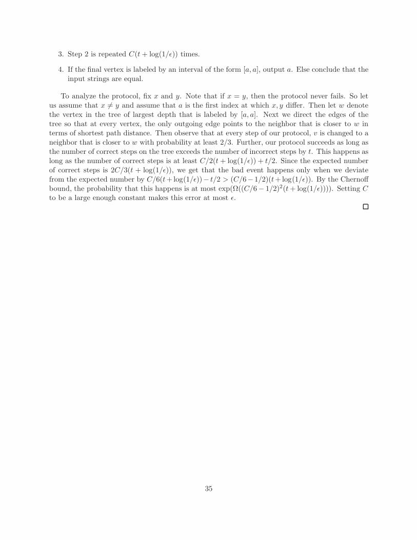
3. Step 2 is repeated C(t+ log(1/ǫ)) times.
4. If the final vertex is labeled by an interval of the form [a, a], output a. Else conclude that theinput strings are equal.
To analyze the protocol, fix x and y. Note that if x = y, then the protocol never fails. So letus assume that x 6= y and assume that a is the first index at which x, y differ. Then let w denotethe vertex in the tree of largest depth that is labeled by [a, a]. Next we direct the edges of thetree so that at every vertex, the only outgoing edge points to the neighbor that is closer to w interms of shortest path distance. Then observe that at every step of our protocol, v is changed to aneighbor that is closer to w with probability at least 2/3. Further, our protocol succeeds as long asthe number of correct steps on the tree exceeds the number of incorrect steps by t. This happens aslong as the number of correct steps is at least C/2(t+ log(1/ǫ)) + t/2. Since the expected numberof correct steps is 2C/3(t + log(1/ǫ)), we get that the bad event happens only when we deviatefrom the expected number by C/6(t+log(1/ǫ))− t/2 > (C/6− 1/2)(t+log(1/ǫ)). By the Chernoffbound, the probability that this happens is at most exp(Ω((C/6− 1/2)2(t+ log(1/ǫ)))). Setting Cto be a large enough constant makes this error at most ǫ.
35
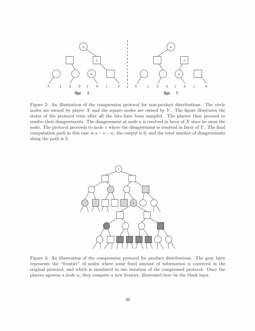
u
v
w
0 1 0 0 1 0 1 0
u
v
w
0 1 0 0 1 0 1 0
P l a y e r X P l a y e r Y
Figure 2: An illustration of the compression protocol for non-product distributions. The circlenodes are owned by player X and the square nodes are owned by Y . The figure illustrates thestates of the protocol trees after all the bits have been sampled. The players then proceed toresolve their disagreements. The disagreement at node u is resolved in favor of X since he owns thenode. The protocol proceeds to node v where the disagreement is resolved in favor of Y . The finalcomputation path in this case is u− v−w, the output is 0, and the total number of disagreementsalong the path is 2.
v
u
Figure 3: An illustration of the compression protocol for product distributions. The gray layerrepresents the “frontier” of nodes where some fixed amount of information is conveyed in theoriginal protocol, and which is simulated in one iteration of the compressed protocol. Once theplayers agreeon a node u, they compute a new frontier, illustrated here by the black layer.
36

Generic Communication Protocol
1. Set v to be the root of the protocol tree.
2. If v is a leaf, the protocol ends and outputs the value in the label of v. Otherwise, theplayer owning v samples a child of v according to the distribution associated with her inputfor v and sends a bit to the other player to indicate which child was sampled.
3. Set v to be the newly sampled node and return to the previous step.
Figure 4: A communication protocol.
Protocol τ
Public Randomness Phase :
1. The players sample j, w−j ∈RJ,W−J using public randomness.
Private Randomness Phase :
1. Px sets xj = x, Py sets yj = y.
2. For every i 6= j, Px samples Xi conditioned on the value of w−j .
3. For every i 6= j, Py samples Yi conditioned on the value of w−j .
4. The players simulate π on the inputs x1, . . . , xn, y1, . . . , yn and output the j’th outputof π.
Figure 5: A protocol simulating π
Protocol γ
Public Randomness Phase :
1. The players sample j, w−j ∈RJ,W−J using public randomness.
Private Randomness Phase :
1. Px sets xj = x, Py sets yj = y.
2. For every i 6= j, Px samples Xi conditioned on the value of w−j .
3. For every i 6= j, Py samples Yi conditioned on the value of w−j .
4. The players simulate π on the inputs x1, . . . , xn, y1, . . . , yn to compute z ∈ ZK .
5. Px computes∑
i 6=j,wi=yif(xi, wi) and sends this sum to Py
6. Py outputs the value of the function as z−∑i 6=j,wi=yif(xi, wi)−
∑
i 6=j,wi=xif(wi, yi).
Figure 6: A protocol simulating π
37

Protocol πr
Sampling Phase :
1. For every non-leaf node w in the tree, the player who owns w samples a child accordingto the distribution given by her input and the public randomness r. This leaves eachplayer with a subtree of the original protocol tree, where each node has out-degree 1or 0 depending on whether or not it is owned by the player.
Path Finding Phase :
1. Set v to be the root of the tree.
2. If v is a leaf, the computation ends with the value of the node. Else, the player towhom v belongs communicates one bit to the other player to indicate which of thechildren was sampled.
3. Set v to the sampled child and return to the previous step.
Figure 7: π restated
Protocol τβ,γ
Public Sampling Phase :
1. Sample r according to the distribution of the public randomness in π.
Correlated Sampling Phase :
1. For every non-leaf node w in the tree, let κw be a uniformly random element of [0, 1]sampled using public randomness.
2. On input x, y, player Px (resp. Py) defines the tree Tx (resp. Ty) in the fol-lowing way: for each node w, Px (resp. Py) includes the edge to the left childif Pr[πr(X,Y ) reaches the left child|πr(X,Y ) reaches w and X = x] > κw (resp. ifPr[πr(X,Y ) reaches the left child|πr(X,Y ) reaches w and Y = y] > κw). Otherwise,the right child is picked.
Path Finding Phase :
1. Each of the players computes the unique path in their trees that leads from the rootto a leaf. The players then use Lemma 3.14, communicating O(log(n/β)) bits tofind the first node at which their respective paths differ, if such a node exists. Theplayer that does not own this node corrects this edge and recomputes his path. Theyrepeatedly correct their paths in this way
√
CC(π) · ICiµ(π)/γ times.
Figure 8: The simulation of π
38
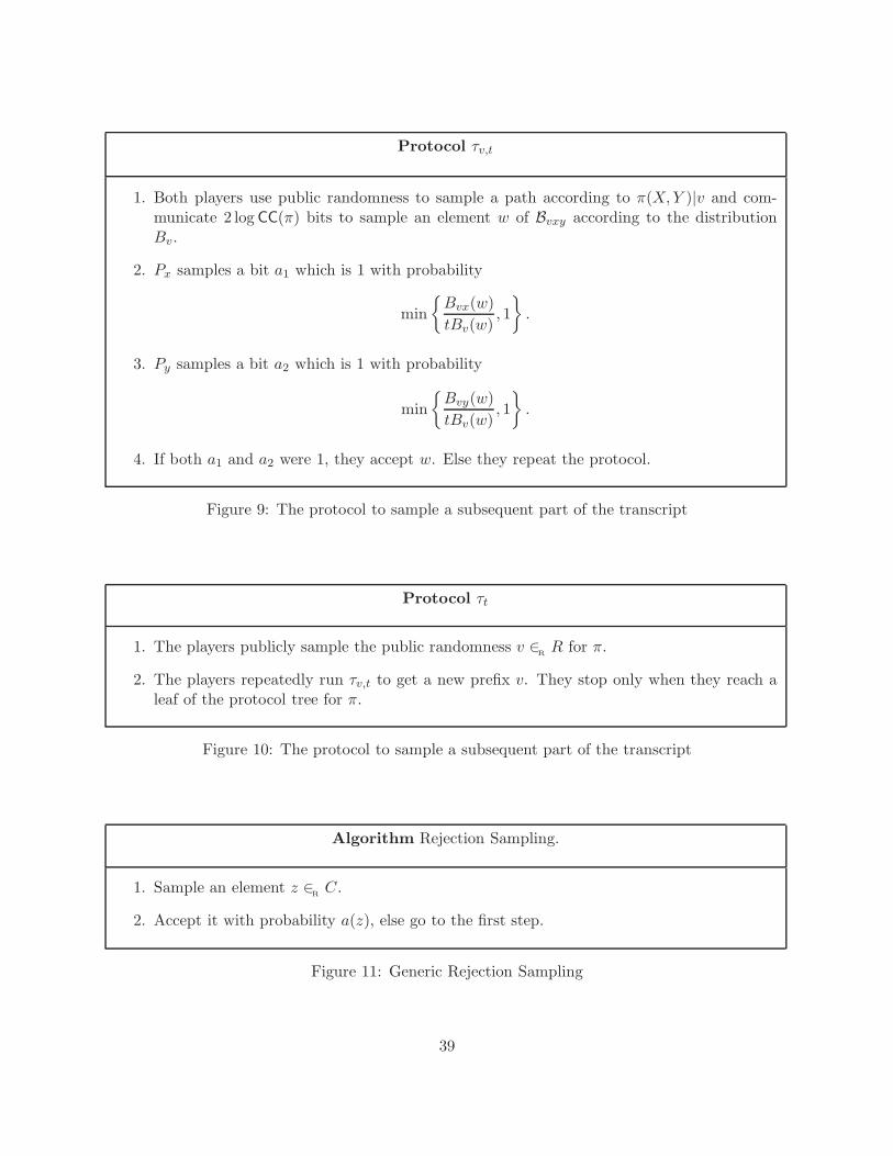
Protocol τv,t
1. Both players use public randomness to sample a path according to π(X,Y )|v and com-municate 2 log CC(π) bits to sample an element w of Bvxy according to the distributionBv.
2. Px samples a bit a1 which is 1 with probability
min
Bvx(w)
tBv(w), 1
.
3. Py samples a bit a2 which is 1 with probability
min
Bvy(w)
tBv(w), 1
.
4. If both a1 and a2 were 1, they accept w. Else they repeat the protocol.
Figure 9: The protocol to sample a subsequent part of the transcript
Protocol τt
1. The players publicly sample the public randomness v ∈RR for π.
2. The players repeatedly run τv,t to get a new prefix v. They stop only when they reach aleaf of the protocol tree for π.
Figure 10: The protocol to sample a subsequent part of the transcript
Algorithm Rejection Sampling.
1. Sample an element z ∈RC.
2. Accept it with probability a(z), else go to the first step.
Figure 11: Generic Rejection Sampling
39


![Acoustic comfort in large dining spaceseprints.whiterose.ac.uk/108552/1/Acoustic Comfort in Large Dining... · XiChen&JianKang:Appliedacoustic [DOI:10.1016/j.apacpust.2016.08.030]](https://img.pdfslide.net/doc/110x75/6038f32cc15e020daa77d58b/acoustic-comfort-in-large-dining-comfort-in-large-dining-xichenjiankangappliedacoustic.jpg)