Hubbard-like Hamiltonians for interacting electrons in s, p and d orbitals

M. E. A. Coury∗

Imperial College London, London SW7 2AZ, United Kingdom andCCFE, Culham Science Centre, Abingdon, Oxfordshire OX14 3DB, United Kingdom

S. L. DudarevCCFE, Culham Science Centre, Abingdon, Oxfordshire OX14 3DB, United Kingdom

W. M. C. FoulkesImperial College London, London SW7 2AZ, United Kingdom

A. P. HorsfieldImperial College London, London SW7 2AZ, United Kingdom

Pui-Wai MaCCFE, Culham Science Centre, Abingdon, Oxfordshire OX14 3DB, United Kingdom

J. S. SpencerImperial College London, London SW7 2AZ, United Kingdom

Hubbard-like Hamiltonians are widely used to describe on-site Coulomb interactions in magneticand strongly-correlated solids, but there is much confusion in the literature about the form theseHamiltonians should take for shells of p and d orbitals. This paper derives the most general s, p andd orbital Hubbard-like Hamiltonians consistent with the relevant symmetries, and presents themin ways convenient for practical calculations. We use the full configuration interaction method tostudy p and d orbital dimers and compare results obtained using the correct Hamiltonian and thecollinear and vector Stoner Hamiltonians. The Stoner Hamiltonians can fail to describe properlythe nature of the ground state, the time evolution of excited states, and the electronic heat capacity.

PACS numbers: 31.15.aq, 31.15.xh, 31.10.+z

I. INTRODUCTION

The starting point for any electronic structure calculationis the Hamiltonian that describes the dynamics of theelectrons. Correlated electron problems are often formu-lated using Hamiltonians that involve only a small num-ber of localized atomic-like orbitals and use an effectiveCoulomb interaction between electrons that is assumedto be short ranged, and thus confined to within atomicsites. However, there is widespread variation in the liter-ature over the form chosen for these Hamiltonians, andthey often do not retain the correct symmetry proper-ties. Here we derive the most general Hamiltonians ofthis type that are rotationally invariant and describe elec-trons populating s, p and d orbitals.

Despite often missing terms, multi-orbital Hamiltonianswith on-site Coulomb interactions have been used suc-cessfully to describe strong correlation effects in sys-tems with narrow bands near the Fermi energy. Ap-plications include studies of metal-insulator transitions1,colossal magnetoresistant manganites2, and d band su-perconductors such as copper oxides3 and iron pnictides4.The Hubbard Hamiltonian has also been used to sim-ulate graphene5,6, where both theory and experimenthave found magnetic ordering in nanoscale structures7,8.However, the lack of consistency in the forms used for

the Hamiltonians is problematic. Indeed, according toDagotto2, “the discussions in the current literature re-garding this issue are somewhat confusing”.The Hubbard Hamiltonian9 is both the simplest and bestknown Hamiltonian of the form we are considering, andis valid for electrons in s orbitals. Hubbard was not thefirst to arrive at this form; two years earlier, in 1961,Anderson wrote down a very similar Hamiltonian10 forelectrons in s orbitals with on-site Coulomb interactions.Furthermore, in the appendix of the same paper, theHamiltonian was extended to two orbitals, introducingthe on-site exchange interaction, J . Unfortunately, thisextra term is not rotationally invariant in spin space.In 1966, Roth11 also considered two orbitals and two pa-rameters, producing a Hamiltonian that is rotationallyinvariant in spin space. In 1969 Caroli et al.12 correctedAnderson’s Hamiltonian for two orbitals, again making itrotationally invariant in spin space. However, the Hamil-tonians of Roth and Caroli et al. do not satisfy rota-tional invariance in orbital space. This was corrected byDworin and Narath in 197013, who produced a Hamilto-nian that is rotationally invariant in both spin and orbitalspace. They generalized the multi-orbital Hamiltonian toinclude all 5 d orbitals, although they only included twoparameters: the on-site Hartree integral, U , and the on-site exchange integral, J .The next contribution to the multi-orbital Hamiltonian

2

was by Lyon-Caen and Cyrot14, who in 1975 considereda two-orbital Hamiltonian for the eg d orbitals. Theyintroduced U0 − U = 2J , where U0 = Vαα,αα is the self-interaction term, U = Vαβ,αβ is the on-site Hartree in-tegral, and J = Vαβ,βα is the on-site exchange integral,important for linking these parameters. Here V is theCoulomb interaction between electrons, and α and β areindices for atomic orbitals. Lyon-Caen and Cyrot also

included the pair excitation, Jc†I1,↑c†I1,↓cI2,↓cI2,↑, where

c† and c are fermionic creation and annihilation opera-tors. The new term moves a pair of electrons from acompletely occupied orbital, 2, on site I, to a completelyunoccupied orbital, 1, on site I. Such double excitationsare common in the literature15–18.In 1978, Castellani et al.19 wrote down the three-orbitalHamiltonian for the t2g d orbitals20 in a very clear andconcise way: its form is exactly what we find here for porbital symmetry. They too make note of the equationU0 − U = 2J and include the double excitation terms.The next major contribution was by Oles and Stollhoff21,who introduced a d orbital Hamiltonian with three inde-pendent parameters. The third parameter, ∆J , repre-sents the difference between the t2g and the eg d orbitalexchange interactions; they estimated ∆J to be 0.15J .In our discussion of d orbitals we adopt their notation.Unfortunately, their Hamiltonian is not rotationally in-variant in orbital space.In 1989, Nolting et al.22 referenced the Hamiltonian pro-posed by Oles and Stollhoff but discarded the double ex-citation terms and ignored the ∆J term. Their Hamilto-nian will be called the vector Stoner Hamiltonian in thispaper. Since then, most papers have used a Hamiltoniansimilar to that of Nolting et al., with only two parame-ters; see for example references 23–25. The vector StonerHamiltonian is often simplified by replacing the rotation-ally invariant moment-squared operator, m2 = m ·m, bym2z, yielding the collinear Stoner Hamiltonian.

The multi-orbital Hamiltonians derived here consistof one-particle hopping (inter-site) integrals and two-electron on-site Coulomb interactions. The on-siteCoulomb interactions for s, p and d orbital symmetriesare presented in a clear tensor notation, as well as interms of physically meaningful, rotationally invariant (inboth orbital and spin space), operators that include allof the terms from the previous papers as well as addi-tional terms of the same order of magnitude that havenot been previously considered. The d orbital Hamil-tonian presented in section II D corrects the d orbitalHamiltonian proposed by Oles and Stollhoff21 by restor-ing full rotational invariance in orbital space. For ans orbital Hamiltonian, the on-site Coulomb interactionsmay be described using one independent parameter. Twoindependent parameters are required for p orbital sym-metry, and three for d orbital symmetry. Furthermore,the method presented can be extended to f and g orbitalsymmetry and generalized to atoms with valence orbitalsof multiple different angular momenta.The use of a restricted basis set and the neglect of the

two-electron inter-site Coulomb interactions means thatscreening effects are missing. Thus, even though the pa-rameters that define the s, p and d Hamiltonians appearas bare on-site Coulomb integrals, screened Coulomb in-tegrals should be used when modelling real systems; thissignificantly reduces the values of the parameters.

Although it is possible to find the on-site Coulomb inte-grals using tables of Slater-Condon parameters26,27 or theclosed forms for the integrals of products of three spheri-cal harmonics found by Gaunt28 and Racah29, the pointof this paper is to remove that layer of obscurity andpresent model Hamiltonians written in a succinct formwith clear physical meaning. The Slater-Condon param-eters and Gaunt integrals were not used in the deriva-tions of the on-site Coulomb interaction Hamiltonianspresented here; however, they did provide an indepen-dent check to confirm that the tensorial forms derivedhere are correct. The link between the spherical har-monics Coulomb integrals, the Slater-Condon parametersand the Racah parameters is explained clearly in30. Thetransformation to cubic harmonics is straightforward; anexample of which has been included for the p-orbitals inSection II C.

We note that Rudzikas31 has derived rotationally invari-ant Hamiltonians for p and d orbital atoms. However, hisderivation is different from ours and his d orbital Hamil-tonian is partially expressed in terms of tensors; the formwe present in this paper is written in terms of physicallymeaningful operators.

The p and d symmetry Hamiltonians are described inSection II (see Appendix B for full derivations) and com-pared with the vector Stoner Hamiltonian. In SectionIII we show the ground state results for both our Hamil-tonian and the vector Stoner Hamiltonian for p and dorbital dimers. We find that, although the results are of-ten similar, there are important qualitative and quanti-tative differences. In Section IV we show the differencesthat emerge when evolving a starting state for a p or-bital dimer under our Hamiltonian and the vector StonerHamiltonian. We also calculate a thermodynamic prop-erty, the electronic heat capacity of a p orbital dimer,and obtain significantly different results when using ourHamiltonian and the vector Stoner Hamiltonian. Theeigenstates of all Hamiltonians are found using the fullconfiguration interaction (FCI) method as implementedin the HANDE code32.

II. THEORY

A. General form of the Hamiltonian

We start with the general many-body Hamiltonian ofelectrons in a solid, expressed in second-quantized formusing a basis of localized one-electron orbitals and ig-noring terms that do not include electronic degrees of

3

freedom33:

H =∑IαJβ

∑σ

tIαJβ c†Iα,σ cJβ,σ

+∑IJKL

∑αβχγ

∑σξ

VIαJβ,KχLγ c†Iα,σ c

†Jβ,ξ cLγ,ξ cKχ,σ.

(1)

Here c†Iα,σ and cIα,σ are creation and annihilation op-erators, respectively, for an electron in orbital α on siteI with spin σ. Upper case Roman letters such as I, J ,K and L refer to atomic sites, the lower case Greek let-ters α, β, χ and γ represent localized orbitals, and σ andζ indicate spin (either up or down). The one-electroncontributions to the Hamiltonian are encapsulated in thetIαJβ term that includes the electronic kinetic energy andelectron-nuclear interaction. The electron-electron inter-action terms are represented by the Coulomb matrix el-ements VIαJβ,KχLγ .We now make two approximations: we only retainelectron-electron Coulomb interactions on-site and we re-strict the basis to a minimal set of localized angular mo-mentum orbitals. Thus we have just one s orbital per sitefor the s-symmetry Hamiltonian, three p orbitals per sitefor the p-symmetry Hamiltonian, and five d orbitals persite for the d-symmetry Hamiltonian. The Hamiltoniancan then be written as follows:

H ≈∑IαJβ

∑σ

tIαJβ c†Iα,σ cJβ,σ

+1

2

∑I

∑αβχγ

∑σξ

V Iαβ,χγ c†Iα,σ c

†Iβ,ξ cIγ,ξ cIχ,σ, (2)

where V Iαβ,χγ = VIαIβ,IχIγ . To improve readability, fromthis point onwards we drop the site index, I, from theCoulomb integrals and creation and annihilation opera-tors as we shall always be referring to on-site Coulombinteractions.The on-site Coulomb interaction, Vαβ,χγ , is a rotation-ally invariant tensor if the atomic-like orbitals are angu-lar momentum eigenstates. To demonstrate this we notethat applying the rotation operator R to an atomic-likeorbital φα of angular momentum ` gives

R|φα〉 =∑β

|φβ〉d`βα(R), (3)

where d`βα(R) is the (2`+1)× (2`+1) matrix that corre-

sponds to the rotation R in the irreducible representationof angular momentum `. By making the change of vari-able x = Rr and x′ = Rr′, it is straightforward to showthat

Vαβ,χγ =

∫drdr′

φ∗ασ(r)φ∗βσ′(r′)φχσ(r)φγσ′(r

′)

|r− r′| ,

=(d`α′α(R)

)∗ (d`β′β(R)

)∗Vα′β′,χ′γ′d

`χ′χ(R)d`γ′γ(R),

(4)

which demonstrates that Vαβ,χγ is indeed a rotationallyinvariant tensor.

B. The one band Hubbard model: s orbitalsymmetry

The Hubbard Hamiltonian is applicable only to one bandmodels where the one orbital per atom has s symmetry.This gives a simple form for the on-site Coulomb inter-action tensor, U0 = Vαα,αα; as there is only one type oforbital, there is only one matrix element. We can use thisresult to simplify the Coulomb interaction part of Eq. (2)and express it in terms of the electron number operator orthe magnetic moment vector operator, defined as follows:

n =∑αζ

c†α,ζ cα,ζ , (5)

m =∑αζζ′

c†α,ζσζζ′ cα,ζ′ , (6)

σζζ′ = (σxζζ′ , σyζζ′ , σ

zζζ′),

where σ are the Pauli spin matrices and the sum over αhas only one term as there is only one spatial orbital forthe s case. Hence

1

2

∑αβχγ

∑σξ

Vαβ,χγ c†α,σ c

†β,ξ cγ,ξ cχ,σ =

1

2U0 : n2 :, (7)

or, equivalently,

1

2

∑αβχγ

∑σξ

Vαβ,χγ c†α,σ c

†β,ξ cγ,ξ cχ,σ = −1

6U0 : m2 :, (8)

where we have use the normal ordering operator, ::, toremove self interactions. The action of this operator is torearrange the creation and annihilation operators suchthat all the creation operators are on the left, withoutadding the anticommutator terms that would be requiredto leave the product of operators unaltered; if the rear-rangement requires an odd number of flips, the normalordering also introduces a sign change. For example

: n2 : =∑αβσζ

: c†α,ζ cα,ζ c†β,σ cβ,σ :,

=∑αβσζ

c†α,ζ c†β,σ cβ,σ cα,ζ . (9)

If the normal ordering operator is not used in Eqs. (7)and (8) then additional one electron terms have to besubtracted to remove the self interaction.The mean-field form of this Hamiltonian has been in-cluded in Appendix A 1.

C. The multi-orbital model Hamiltonian: p orbitalsymmetry

Consider the case where the local orbitals, α, β, χ and γappearing in Eq. (4) are real cubic harmonic p orbitalswith angular dependence x/r, y/r, and z/r. In this case

4

the rotation matrices, d`α′α(R), are simply 3 × 3 Carte-sian rotation matrices. This makes Vαβ,χγ a rotationallyinvariant fourth-rank Cartesian tensor, the general formof which is34,

Vαβ,χγ = Uδαχδβγ + Jδαγδβχ + J ′δαβδχγ , (10)

where U = Vαβ,αβ , J = Vαβ,βα and J ′ = Vαα,ββ , withα 6= β. By examination of the integral in Eq. (4), wenote that the Coulomb tensor has an additional symme-try when the orbitals are real (as are the cubic harmonic porbitals), namely Vαβ,χγ = Vχβ,αγ and Vαβ,χγ = Vαγ,χβ ,and hence J must be equal to J ′. Thus we find

Vαβ,χγ = Uδαχδβγ + J (δαγδβχ + δαβδχγ) . (11)

This recovers the well known equation U0 = U + 2J ,where U0 = Vαα,αα

14,19, and shows that the most gen-eral cubic p orbital interaction Hamiltonian is defined byexactly two independent parameters35. In Appendix B 1we give a full derivation of Eq. (11) using representationtheory.In passing we observe that symmetric fourth-rankisotropic tensors can be found in other areas of physics,such as the stiffness tensor in isotropic elasticity theory36

Ciklm = λδikδlm + µ(δilδkm + δimδkl), (12)

where λ is the Lame coefficient and µ is the shear mod-ulus.Transforming Eq. (11) into a basis of complex sphericalharmonic p orbitals with angular dependence of the formY`m(θ, φ) is straightforward. We write Vmm′′,m′m′′′ =∑αβχγ l

∗mαl

∗m′′βlm′χlm′′′γVαβ,χγ , where lmα is defined by

psphm =∑α

lmαpα, (13)

and has the following values

[lmα] =

1√2− i√

20

0 0 1− 1√

2− i√

20

. (14)

The result of applying this transformation is

Vmm′′,m′m′′′ =Uδmm′δm′′m′′′ + Jδmm′′′δm′′m′

+ (−1)m+m′Jδ−mm′′δ−m′m′′′ , (15)

where m, m′, m′′ and m′′′ are spherical harmonics indicesgoing from −1 to +1, U = V10,10, and J = V10,01.Using Eq. (11) as a convenient starting point, it isstraightforward to rewrite the on-site Coulomb Hamil-tonian in terms of rotationally invariant operators:31

1

2

∑αβχγ

∑σξ

Vαβ,χγ c†α,σ c

†β,ξ cγ,ξ cχ,σ

=1

2

((U − J) : n2 : −J : m2 : −J : L2 :

), (16)

where the vector angular momentum operator for p or-bitals on site I is defined to be

L = i∑αβσ

(ε1βα, ε2βα, ε3βα)c†α,σ cβ,σ, (17)

and εµβα is the three-dimensional Levi-Civita symbol.An equivalent expression is

1

2

∑αβχγ

∑σζ

Vαβ,χγ c†α,σ c

†β,ζ cγ,ζ cχ,σ

=1

2

((U − 1

2J

): n2 : −1

2J : m2 :

+ J∑αβ

: (nαβ)2

:

), (18)

where the final term corresponds to on-site electronhopping37,

nαβ =∑σ

c†α,σ cβ,σ. (19)

Eq. (16) embodies Hund’s rules for an atom. By mak-

ing the substitution m = 2S, we see that the spin ismaximized first (prefactor −2J) and then the angularmomentum is maximized (prefactor − 1

2J).

The mean-field form of the above p orbital Hamiltonianis given in Appendix A 2.

D. The multi-orbital model Hamiltonian: d orbitalsymmetry

The on-site Coulomb interaction for cubic harmonic dorbitals can be expressed as

Vαβ,χγ =1

2

(Uδαχδβγ

+

(J +

5

2∆J

)(δαγδβχ + δαβδγχ)

− 48∆J∑abdt

ξαabξβbdξχdtξγta

), (20)

5

where ξ is a five-component vector of traceless symmetric3× 3 transformation matrices defined as follows

[ξ1ab] =

−1

2√3

0 0

0 − 12√3

0

0 0 1√3

,

[ξ2ab] =

0 0 12

0 0 012 0 0

,

[ξ3ab] =

0 0 00 0 1

20 1

2 0

,

[ξ4ab] =

0 12 0

12 0 00 0 0

,

[ξ5ab] =

12 0 00 − 1

2 00 0 0

. (21)

We use the convention that index numbers (1, 2, 3, 4, 5)correspond to the d orbitals (3z2−r2, zx, yz, xy, x2−y2).See Appendix B 2 for a derivation of Eq. (21) using rep-resentation theory. We have chosen U to be the Hartreeterm between the t2g orbitals, J to be the average of theexchange integral between the eg and t2g orbitals, and∆J to be the difference between the exchange integralsfor eg and t2g. That is, U = V(zx)(yz),(zx)(yz), J =12

(V(zx)(yz),(yz)(zx) + V(3z2−r2)(x2−y2),(x2−y2)(3z2−r2)

),

and ∆J = V(3z2−r2)(x2−y2),(x2−y2)(3z2−r2) −V(zx)(yz),(yz)(zx). This choice of parameters is the

same as was used by Oles and Stollhoff21; Eq. (20)generalizes their result and restores rotational invariancein orbital space. Note that, in the mean field, the on-siteblock of the density matrix in a cubic solid is diagonal;this will cause the mean-field version of Eq. 22) to reduceto that of Oles and Stollhoff21. However the presenceof interfaces, vacancies or interstitials will break thecubic symmetry make the on-site blocks of the densitymatrix non-diagonal. Therefore the use of the completeHamiltonian is recommended in mean-field calculationsfor systems that do not have cubic symmetry.Rewriting Eq. (20) in terms of rotationally invariant op-erators gives

Vtot =1

2

[(U − 1

2J + 5∆J

): n2 : −1

2(J − 6∆J) : m2 :

+ (J − 6∆J)∑αβ

: (nαβ)2

: +2

3∆J : Q2 :

], (22)

where Q2 is the on-site quadrupole operator squared.The quadrupole operator for a single electron is definedas

Qµν =1

2

(LµLν + LνLµ

)− 1

3δµνL

2. (23)

The quadrupole operator for a system of many electronsis obtained by summing the operators for each electron.

Since each term in the sum acts on the coordinates ofone electron only, the operators Lµ and Lν appearing inthat term measure the angular momentum of one elec-tron only, not the whole system. More detail on the Q2

operator is included in Appendix C. Eq. (22) is similarin form to that found in Rudzikas31, the difference beingthat our Hamiltonian is expressed in terms of physicallymeaningful operators.The mean-field form of this Hamiltonian is given in Ap-pendix A 3.

E. Comparison with the Stoner Hamiltonian

The Stoner Hamiltonian for p and d orbital atoms, asgenerally defined in the literature, has the following formfor the on-site Coulomb interaction:25

VStoner =1

2

(U − 1

2J

): n2 : −1

4J : m2

z :, (24)

where J , in this many-body context, is the Stoner pa-rameter, I. However, in the mean field, the Stoner pa-rameter should not be taken to be equal to J due to theself-interaction error; see reference38. This form clearlybreaks rotational symmetry in spin space, which can berestored by substituting : m2

z : with : m2 :

Vm2 Stoner =1

2

(U − 1

2J

): n2 : −1

4J : m2 : . (25)

In this paper we will compare our Hamiltonians, Eqs. (18)and (22), with Eq. (25), which we shall call the vectoror m2 Stoner Hamiltonian. By starting with the vectorStoner Hamiltonian and working backwards, it is possibleto find the corresponding tensorial form of the Coulombinteraction:

V m2 Stonerαβ,χγ = Uδαχδβγ + Jδαγδβχ. (26)

This is very similar to the tensorial form for the p-caseCoulomb interaction, Eq. (11), except that it is missinga term, Jδαβδγχ. The lack of this term means that thevector Stoner Hamiltonian does not respect the symme-try between pairs αχ and βγ evident from the form of

the integral in Eq. (4), i.e., V m2 Stonerχβ,αγ 6= V m2 Stoner

αβ,χγ . Aswe shall see later, this omission changes the computedresults.

III. GROUND STATE RESULTS

A. Simulation setup

Here we investigate the eigenstates of dimers using bothour Hamiltonians, Eqs. (18) and (22), and the vectorStoner Hamiltonian, Eq. (25). We employ a restrictedbasis with a single set of s, p and d orbitals for the s, p

6

and d Hamiltonians respectively. We perform FCI cal-culations using the HANDE32 computer program to findexact eigenstates of the model Hamiltonians. The Lanc-zos algorithm was used to calculate the lowest 40 wave-functions for our Hamiltonian, more than sufficient tofind the correct ground state wavefunction, while the fullspectrum was calculated for the vector Stoner Hamilto-nian.The single particle contribution to the Hamiltonian forall models (the hopping matrix) is defined for a dimeraligned along the z-axis: in this case it is only non-zerobetween orbitals of the same type, whether on the samesite or on different sites. The sigma hopping integral,|tσ|, was set to 1 to define the energy scale. The otherhopping matrix elements follow the canonical relationssuggested by Andersen39, and we use the values of Paxtonand Finnis40: ppσ : ppπ = 2 : −1 for p orbitals, andddσ : ddπ : ddδ = −6 : 4 : −1 for d orbitals.The directionally averaged magnetic correlation betweenthe two sites has been calculated for the ground state.If positive it shows that the atoms are ferromagneticallycorrelated (spins parallel on both sites) and if it is neg-ative it shows that the atoms are antiferromagneticallycorrelated (spins antiparallel between sites). The correla-tion between components of spin projected onto a direc-tion described by angles θ and φ, in spherical coordinates,is defined as follows

Cθφ = 〈: m1θφm

2θφ :〉, (27)

where the :: is the normal ordering operator, used toremove self-interaction, and

mIθφ =

∑αξξ′

σθφξξ′ c†Iα,ξ cIα,ξ′ , (28)

σθφξξ′ = σzξξ′ cos θ + σxξξ′ sin θ cosφ+ σyξξ′ sin θ sinφ.

The magnetic correlation averaged over solid angle is

Cavg =1

3〈: m1.m2 :〉. (29)

B. Ground state: p orbital dimer

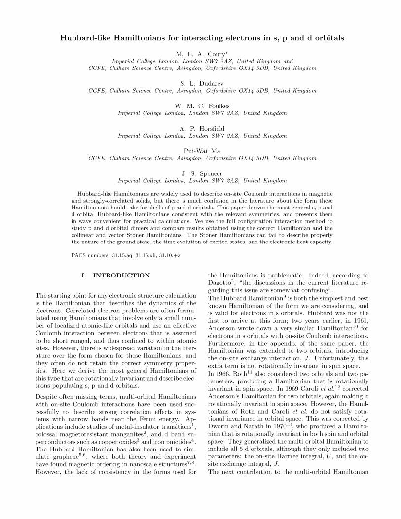
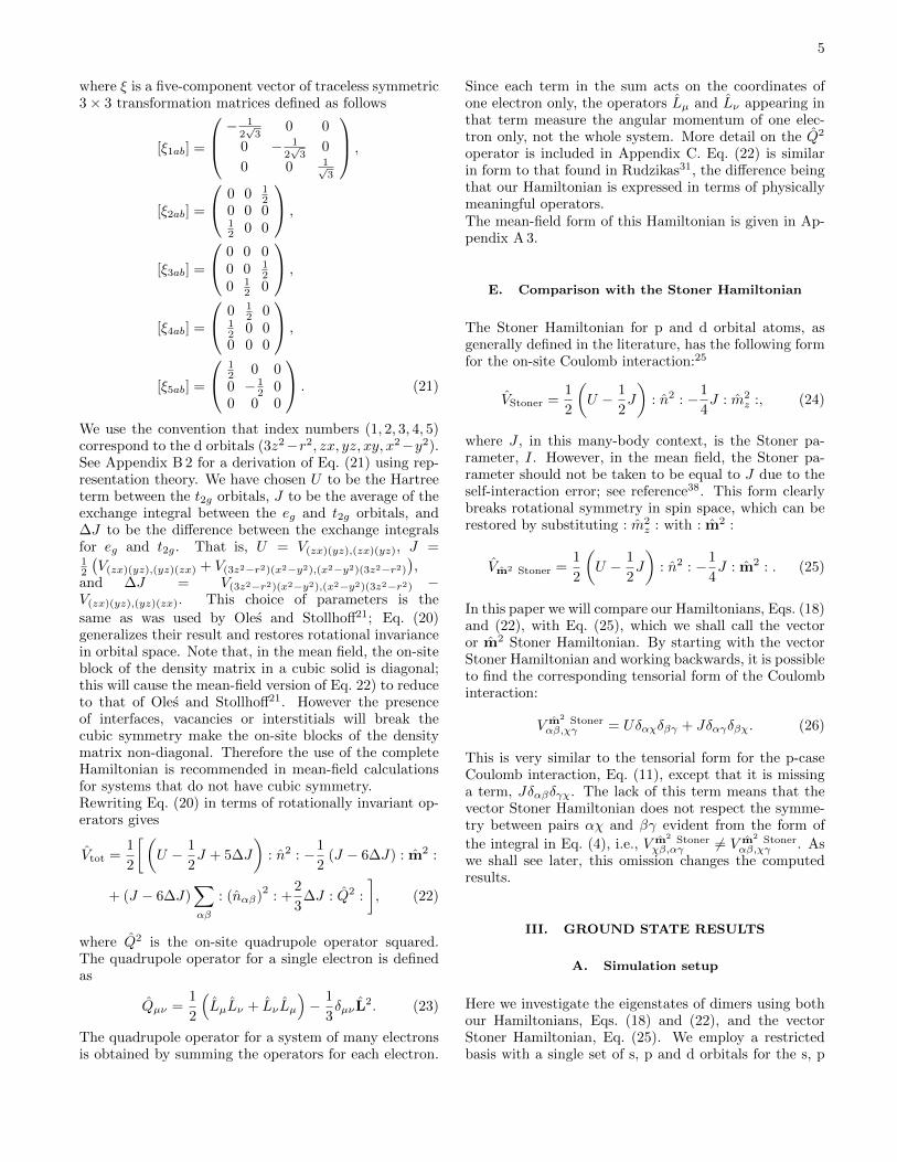
The ground states of our Hamiltonian and the vectorStoner Hamiltonian have been found to be rather similarfor 2, 6 and 10 electrons split over the p orbital dimer,but qualitatively different for 4 and 8 electrons. The mag-netic correlation between the two atoms for 4 electrons isshown in Fig. 1. The symmetries of the wavefunctions41

are indicated on the graph by the notation 2S+1Λ±u/g: the

± is only used for Lz = 0 (i.e. Σ states) and correspondsto the sign change after a reflection in a plane parallelto the axis of the dimer; the u/g term refers to ungerade(odd) and gerade (even) and corresponds to a reflectionthrough the midpoint of the dimer; Λ is the symbol cor-responding to the total value for Lz (e.g. Lz = 1 is Π,Lz = 2 is ∆, Lz = 3 is Φ, Lz = 4 is Γ); and S is the

2 4 6 8 10U/|t|

0.5

1.0

1.5

2.0

2.5

J/|t|

−2.5

−2.0

−1.5

−1.0

−0.5

0.0

0.5

1.0

13 〈:m1 .m

2:〉

FIG. 1: The magnetic correlation between two p-shellatoms, each with 2 electrons, for a large range of

parameters U/|t| and J/|t|, where t is the sigma bondhopping. The different regions of the graph are labeledby the symmetry of the ground state. The top graph isgenerated from our Hamiltonian and the bottom from

the vector Stoner Hamiltonian. The bottom graph has aregion with symmetry 3Σ−g extending a long way up theJ axis, which is not present in the ground state of ourHamiltonian. The bottom graph also includes a regionwith two degenerate states with symmetries 1∆g and

1Σ+g ; this degeneracy is broken when our Hamiltonian is

used.

total spin. The differences between the ground statesof our Hamiltonian and the vector Stoner Hamiltonianshown in Fig. 1 are as follows: the ground-state wave-function of the vector Stoner Hamiltonian has a regionwith 3Σ−g symmetry extending far up the J axis, which

is not present for our Hamiltonian; the region with 1∆g

symmetry is doubly degenerate for our Hamiltonian, astotal Lz = ±2, whereas for the Stoner Hamiltonian it istriply degenerate, as it is also degenerate with the state

7

of symmetry 1Σ+g (this state appears at a higher energy

for our Hamiltonian).

C. Ground state: d orbital dimer

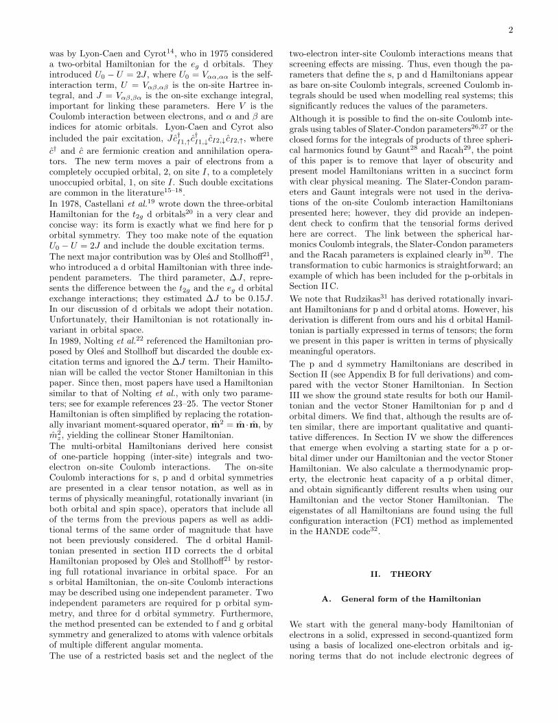
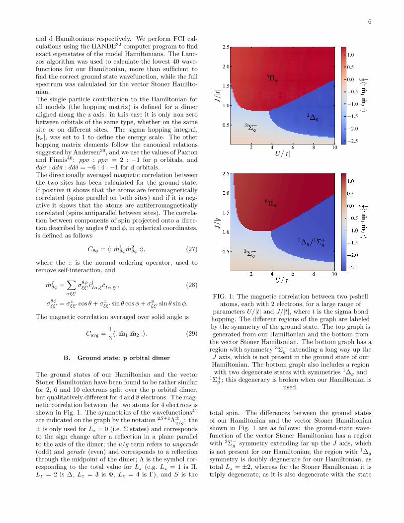
The ground states of our Hamiltonian and vector StonerHamiltonian have been found to be rather similar for 2, 4,6, 14, and 18 electrons split over the d orbital dimer when∆J is small. The simulations for 10 electrons were notcarried out as they are too computationally expensive.Qualitative differences were found for 8 and 12 electrons;for an example see Fig. 2, which shows the magnetic cor-relation between two atoms in the ground state of thed-shell dimer with 6 electrons per atom. From Fig. 2 wesee that the results for our Hamiltonian with ∆J/|t| = 0.0(top graph) and with a small value of ∆J/|t| = 0.1 (mid-dle graph) are qualitatively different from those for thevector Stoner Hamiltonian (bottom graph). The vectorStoner Hamiltonian makes the 1Γg and 1Σ+

g states de-generate, which is not the case for our Hamiltonian. Thelargest differences are between the ∆J/|t| = 0.1 graphand the vector Stoner Hamiltonian: new regions withsymmetry 1Σ+

g , 3Φg and 5Σ−g appear, and the region with

symmetry 3Σ−g almost disappears. This shows that theinclusion of the quadrupole term in Eq. (22) can make aqualitative difference to the ground state.

IV. EXCITED STATE RESULTS

Differences between our Hamiltonian and the vectorStoner Hamiltonian are also observed for excited states.Here we present three examples, one demonstrating ex-plicitly the effect of the pair hopping, one showing moregeneral differences in the excited states through a cal-culation of the electronic heat capacity as a function oftemperature, and one showing a difference in the spindynamics of a collinear and a non-collinear Hamiltonian.The full spectrum of eigenstates was calculated for all ofthese examples.

A. Pair hopping

The pair hopping term, J∑αβσσ′ c

†α,σ c

†α,σ′ cβ,σ′ cβ,σ =

J∑αβ : (nαβ)

2:, is found in both our p and d or-

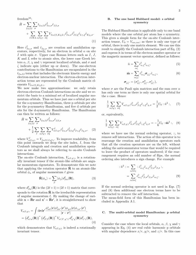
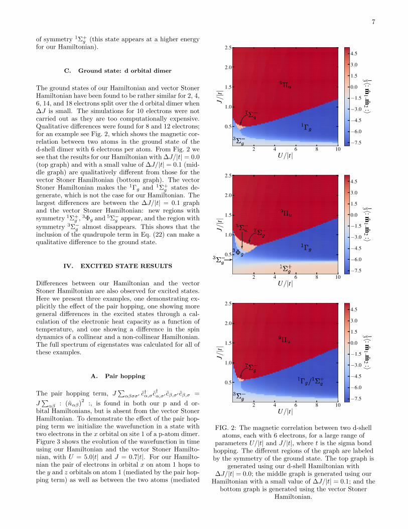
bital Hamiltonians, but is absent from the vector StonerHamiltonian. To demonstrate the effect of the pair hop-ping term we initialize the wavefunction in a state withtwo electrons in the x orbital on site 1 of a p-atom dimer.Figure 3 shows the evolution of the wavefunction in timeusing our Hamiltonian and the vector Stoner Hamilto-nian, with U = 5.0|t| and J = 0.7|t|. For our Hamilto-nian the pair of electrons in orbital x on atom 1 hops tothe y and z orbitals on atom 1 (mediated by the pair hop-ping term) as well as between the two atoms (mediated

2 4 6 8 10U/|t|

0.5

1.0

1.5

2.0

2.5

J/|t|

−7.5

−6.0

−4.5

−3.0

−1.5

0.0

1.5

3.0

4.5

13 〈:m1 .m

2:〉

2 4 6 8 10U/|t|

0.5

1.0

1.5

2.0

2.5

J/|t|

−7.5

−6.0

−4.5

−3.0

−1.5

0.0

1.5

3.0

4.5

13 〈:m1 .m

2:〉

2 4 6 8 10U/|t|

0.5

1.0

1.5

2.0

2.5

J/|t|

−7.5

−6.0

−4.5

−3.0

−1.5

0.0

1.5

3.0

4.5

13 〈:m1 .m

2:〉

FIG. 2: The magnetic correlation between two d-shellatoms, each with 6 electrons, for a large range of

parameters U/|t| and J/|t|, where t is the sigma bondhopping. The different regions of the graph are labeledby the symmetry of the ground state. The top graph is

generated using our d-shell Hamiltonian with∆J/|t| = 0.0; the middle graph is generated using our

Hamiltonian with a small value of ∆J/|t| = 0.1; and thebottom graph is generated using the vector Stoner

Hamiltonian.

8

0 2 4 6 8 10 12 14 16time(h/|t|)

0.0

0.5

1.0

1.5

2.0〈n

Iα〉

1x1y1z2x2y2z

0 2 4 6 8 10 12 14 16time(h/|t|)

0.0

0.5

1.0

1.5

2.0

〈nIα〉

1x1y1z2x2y2z

FIG. 3: The time evolution under our Hamiltonian(top) and the vector Stoner Hamiltonian (bottom) of astarting state with two electrons in 1x, the x orbital on

atom 1, of a p-atom dimer with U = 5.0|t| andJ = 0.7|t|. We see that the two electrons in 1x are ableto hop into 1y and 1z when the wavefunction is evolvedusing our Hamiltonian but not when it is evolved using

the vector Stoner Hamiltonian.

by the single electron hopping term). The result is thatthere is a finite probability of finding the pair of electronsin any of the x, y and z orbitals on either atom. However,for the vector Stoner Hamiltonian, the two electrons inthe x orbital on site 1 are unable to hop into the y andz orbitals on atom 1; they are only able to hop to the xorbital on atom 2. This means tha there is no possibilityof observing the pair of electrons in the y or z orbitalson either atom.

10−3 10−2 10−1 100 101 102

kBT/|t|0.0

0.1

0.2

0.3

0.4

0.5

0.6

0.7

0.8

CV/(

k BN

a)

p orbital HamiltonianStoner Hamiltonian

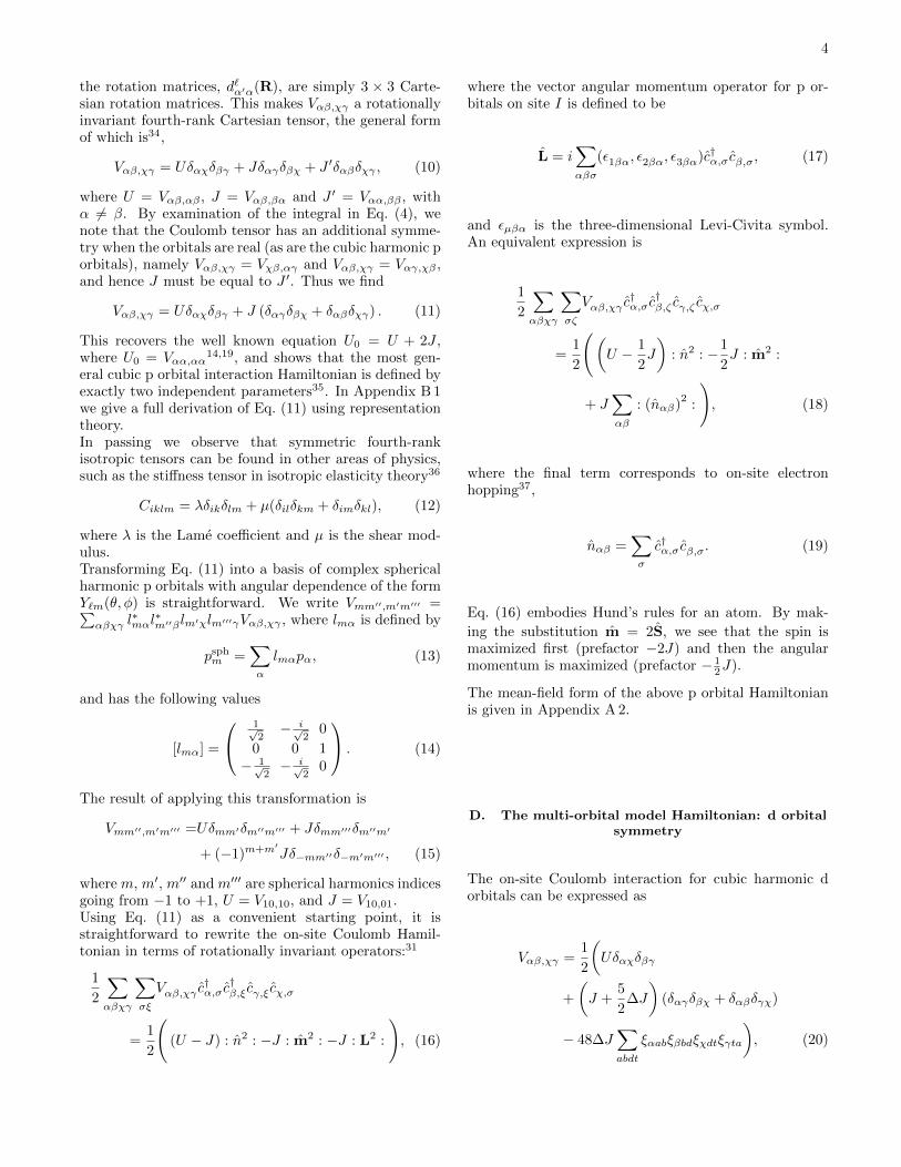
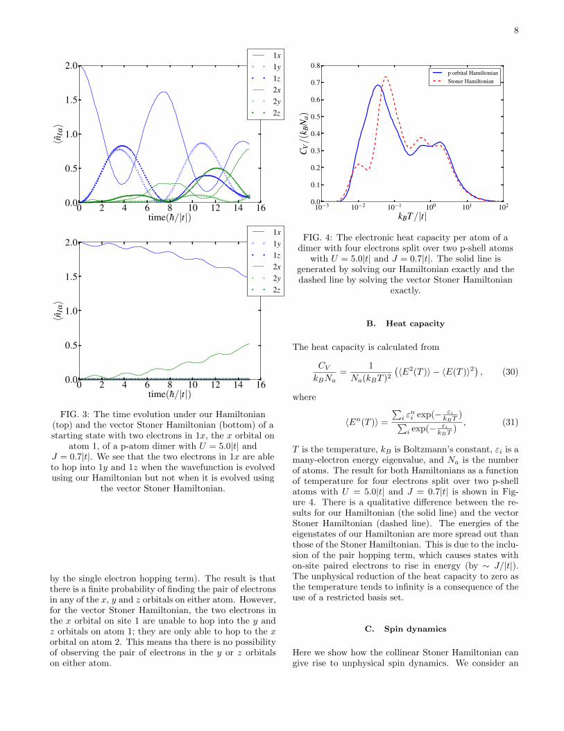
FIG. 4: The electronic heat capacity per atom of adimer with four electrons split over two p-shell atoms

with U = 5.0|t| and J = 0.7|t|. The solid line isgenerated by solving our Hamiltonian exactly and thedashed line by solving the vector Stoner Hamiltonian

exactly.

B. Heat capacity

The heat capacity is calculated from

CVkBNa

=1

Na(kBT )2(〈E2(T )〉 − 〈E(T )〉2

), (30)

where

〈En(T )〉 =

∑i εni exp(− εi

kBT)∑

i exp(− εikBT

), (31)

T is the temperature, kB is Boltzmann’s constant, εi is amany-electron energy eigenvalue, and Na is the numberof atoms. The result for both Hamiltonians as a functionof temperature for four electrons split over two p-shellatoms with U = 5.0|t| and J = 0.7|t| is shown in Fig-ure 4. There is a qualitative difference between the re-sults for our Hamiltonian (the solid line) and the vectorStoner Hamiltonian (dashed line). The energies of theeigenstates of our Hamiltonian are more spread out thanthose of the Stoner Hamiltonian. This is due to the inclu-sion of the pair hopping term, which causes states withon-site paired electrons to rise in energy (by ∼ J/|t|).The unphysical reduction of the heat capacity to zero asthe temperature tends to infinity is a consequence of theuse of a restricted basis set.

C. Spin dynamics

Here we show how the collinear Stoner Hamiltonian cangive rise to unphysical spin dynamics. We consider an

9

Sz = +1 triplet with both electrons on one of the twop orbital atoms, |Ψ〉 = |T+1〉. Written as linear com-binations of two-electron Slater determinants, the threestates in the triplet are

|T+1〉 =1√2

(−|1x ↑ 1y ↑〉+ |2x ↑ 2y ↑〉) ,

|T−1〉 =1√2

(−|1x ↓ 1y ↓〉+ |2x ↓ 2y ↓〉) ,

|T0〉 =− 1√2

(|1x ↓ 1y ↑〉+ |1x ↑ 1y ↓〉)

+1√2

(|2x ↓ 2y ↑〉+ |2x ↑ 2y ↓〉) . (32)

These states are simultaneously eigenstates of thecollinear Stoner Hamiltonian, the vector Stoner Hamil-tonian, and our p-case Hamiltonian. They are degener-ate, with eigenvalue U − J , for both our p-case Hamil-tonian and for the vector Stoner Hamiltonian. For thecollinear Stoner Hamiltonian the states |T+1〉 and |T−1〉have eigenvalue U − J whereas state |T0〉 has eigenvalueU . This means that the degeneracy of this triplet is bro-ken in the collinear Stoner Hamiltonian. We now rotate|Ψ〉 in spin space so that the spins are aligned with thex-axis, i.e. Sx = +1,

|Ψrot〉 =1

2(|T+1〉+ |T−1〉) +

1√2|T0〉. (33)

|Ψrot〉 is still an eigenstate, with eigenvalue U−J , of boththe vector Stoner Hamiltonian and our Hamiltonian, butit is no longer an eigenstate of the collinear Stoner Hamil-tonian. The wavefunction |Ψrot〉 evolves in time as

|Ψtot(τ)〉 = e−iHτh |Ψtot(0)〉, (34)

=

e−i(U−J)τ

h

(1

2(|T+1〉+ |T−1〉) +

e−iJτh√2|T0〉

)︸ ︷︷ ︸

collinear Stoner Hamiltonian

,

e−i(U−J)τ

h

(1

2(|T+1〉+ |T−1〉) +

1√2|T0〉

)︸ ︷︷ ︸

m2 Stoner and our Hamiltonian

,

where τ is time. If we take the expectation value of themagnetic moment on each site using the collinear StonerHamiltonian, we find

〈Ψrot(τ)|m1x|Ψrot(τ)〉 = 〈Ψrot(τ)|m2x|Ψrot(τ)〉 = cos

(Jτ

h

),

〈Ψrot(τ)|m1y|Ψrot(τ)〉 = 〈Ψrot(τ)|m2y|Ψrot(τ)〉 = 0,

〈Ψrot(τ)|m1z|Ψrot(τ)〉 = 〈Ψrot(τ)|m2z|Ψrot(τ)〉 = 0.(35)

In contrast, using the vector Stoner Hamiltonian or ourp-shell Hamiltonian, the expectation value of the mag-netic moment is independent of time, equal to (1, 0, 0)in vector format. This demonstrates that calculationsof spin dynamics using the collinear Stoner Hamiltoniancan give rise to unphysical oscillations of the magneticmoments.

V. CONCLUSION

We have established the correct form of the multi-orbitalmodel Hamiltonian with on-site Coulomb interactions foratoms with valence shells of s, p and d orbitals. Themethodology used may be extended to atoms with f andg shells, and to atoms with valence orbitals of severaldifferent angular momenta. The results presented showthat there are important differences between our p- andd-shell Hamiltonians and the vector Stoner Hamiltonian.The vector Stoner Hamiltonian misses both the pair hop-ping term, which is present in our p and d orbital Hamil-tonians, and the quadrupole term, which is present in ourd orbital Hamiltonian. The pair hopping term pushesstates with pairs of electrons up in energy, whereas themagnetism term pulls states with local magnetic mo-ments down in energy. The pair hopping term has thelargest effect on the ground state for p orbitals with 2and 4 electrons per atom and for d orbitals with 4 and6 electrons per atom, for J/|t| < 2. This is because thenumber of possible determinants with paired electronson site is large for these filling factors and the low ly-ing states can be separated based on this. At values ofJ/|t| > 2 the magnetism becomes the dominant effectupon the selection of the ground state and the differencebetween the ground state of our Hamiltonian and thatof the vector Stoner Hamiltonian becomes small. How-ever, the differences are rather more pronounced for theexcited states. This is evidenced by the hopping of pairsof electrons between orbitals on the same site, which isallowed by our Hamiltonian but not by the vector StonerHamiltonian, and in differences in the electronic heat ca-pacity as a function of temperature. We also find clearevidence that the collinear Stoner Hamiltonian is inap-propriate for use in describing spin dynamics as it breaksrotational symmetry in spin space. We would expect sim-ilar problems when using collinear time dependent DFTsimulations to model spin dynamics.

ACKNOWLEDGEMENTS

The authors would like to thank Toby Wiseman for helpwith the representation theory and Dimitri Vvedensky,David M. Edwards, Cyrille Barreteau and Daniel Span-jaard for stimulating discussions. M. E. A. Coury wassupported through a studentship in the Centre for Doc-toral Training on Theory and Simulation of Materials atImperial College funded by EPSRC under grant num-ber EP/G036888/1. This work was part-funded by theEuroFusion Consortium, and has received funding fromEuratom research and training programme 20142018 un-der Grant Agreement No. 633053, and funding from theRCUK Energy Programme (Grant No. EP/I501045).The views and opinions expressed herein do not neces-sarily reflect those of the European Commission. Theauthors acknowledge support from the Thomas YoungCentre under grant TYC-101

10

Appendix A: Mean-field Hamiltonians

1. The one band Hubbard model: s orbitalsymmetry

Application of the mean-field approximation42 to the on-site Coulomb interaction part of the Hubbard Hamilto-nian with s orbital symmetry, Eq. (7), yields the follow-ing,

VMF =U0

(〈n〉n−

∑σζ

〈c†σ cζ〉c†ζ cσ

), (A1)

for which the total energy is

ECoulombMF =

1

2U0

〈n〉2 −∑σζ

〈c†σ cζ〉〈c†ζ cσ〉

, (A2)

where the double counting correction has been included.Equivalently, applying the mean-field approximation toEq. (8) yields the following,

VMF =1

3U0

(2〈n〉n− 〈m〉.m−

∑σζ

〈c†σ cζ〉c†ζ cσ

), (A3)

for which the total energy is

ECoulombMF =

1

6U0

2〈n〉2 − 〈m〉2 −∑σζ

〈c†σ cζ〉〈c†ζ cσ〉

,

(A4)

where again the double counting correction has been in-cluded.

2. The multi-orbital model Hamiltonian: p orbitalsymmetry

Application of the mean-field approximation42 to themodel Hamiltonian with p orbital symmetry, Eq. (18),yields the following,

VMF =

(U − J

2

)〈n〉n− J

2〈m〉.m

+∑αβ

J

(〈nαβ〉nβα + 〈nαβ〉nαβ

)

−∑αβσζ

(U〈c†ασ cβζ〉c

†βζ cασ + J〈c†ασ cβζ〉c

†αζ cβσ

),

(A5)

for which the total energy is

ECoulombMF =

1

2

(U − J

2

)〈n〉2 − J

4〈m〉2

+∑αβ

J

2

(〈nαβ〉〈nβα〉+ 〈nαβ〉2

)−∑αβσζ

(U

2〈c†ασ cβζ〉〈c

†βζ cασ〉

+J

2〈c†ασ cβζ〉〈c

†αζ cβσ〉

), (A6)

where the double counting correction has been included.

3. The multi-orbital model Hamiltonian: d-orbitalsymmetry

Application of the mean-field approximation42 to themodel Hamiltonian with d-orbital symmetry, Eq. (22),yields the following,

VMF =

(U − 1

2J + 2∆J

)〈n〉n− J

2〈m〉.m

+ (J − 6∆J)∑αβ

(〈nαβ〉nβα + 〈nαβ〉nαβ

)+

2

3∆J

∑µν

〈Qµν〉Qνµ

−∑αβσζ

(U〈c†ασ cβζ〉c

†βζ cασ + J〈c†ασ cβζ〉c

†αζ cβσ

)+ 48∆J

∑αβγχσζ

∑stuv

ξαstξβtuξχuvξγvs〈c†ασ cγζ〉c†βζ cχσ,

(A7)

for which the total energy is

ECoulombMF =

1

2

(U − 1

2J + 2∆J

)〈n〉2 − J

4〈m〉2

+∑αβ

J − 6∆J

2

(〈nαβ〉〈nβα〉+ 〈nαβ〉2

)+

1

3∆J

∑µν

〈Qµν〉〈Qνµ〉

−∑αβσζ

(U

2〈c†ασ cβζ〉〈c

†βζ cασ〉

+J

2〈c†ασ cβζ〉〈c

†αζ cβσ〉

)+ 24∆J

∑αβγχσζ

∑stuv

ξαstξβtuξχuvξγvs

× 〈c†ασ cγζ〉〈c†βζ cχσ〉, (A8)

where the double counting correction has been included.

11

Appendix B: Representation theory

1. p orbital symmetry

As a precursor to our treatment of the d case in AppendixB 2, we use representation theory43 to derive Eq. (11) forcubic harmonic p orbitals. First we define the follow-ing irreducible objects: “0” is a scalar, “1” is a three-dimensional vector, “2” is a 3 × 3 symmetric tracelesssecond-rank tensor, “3” is a third-rank tensor consistingof three “2”s, and “4” is a fourth-rank tensor consisting ofthree “3”s. The Coulomb interaction Vαβ,γδ transformsas a tensor product of four “1”s, 1 ⊗ 1 ⊗ 1 ⊗ 1, but weknow also that it must be isotropic and that from theabove irreducible objects only the “0” is isotropic.Objects such as 1 ⊗ 1, represented as Aij , may be ex-panded just as in the addition of angular momentum:

1⊗ 1 = 0⊕ 1⊕ 2, (B1)

where “0” is a scalar, s =∑ij Aijδij , “1” is a vector,

vi =∑jk Ajkεijk, and “2” is a traceless symmetric ten-

sor, Mij = 12 (Aij + Aji) − 1

3δij(∑klAklδkl). The reader

may be more familiar with combinations of angular mo-mentum. In the language of angular momentum, thetransformation properties of a tensor product of two ob-jects of angular momentum with l = 1 are described bya 9× 9 matrix, which is block diagonalisable into a 1× 1matrix (which describes the transformations of an l = 0object), a 3× 3 matrix (which describes the transforma-tions of an l = 1 object), and a 5 × 5 matrix (whichdescribes the transformations of an l = 2 object). In theangular momentum representation the matrix elementsare complex. Here we are using cubic harmonics and thematrix elements are real. Similarly 1⊗ 1⊗ 1⊗ 1 may beexpanded out as:

1⊗ 1⊗ 1⊗ 1 = (1⊗ 1)⊗ (1⊗ 1),

= (0⊕ 1⊕ 2)⊗ (0⊕ 1⊕ 2),

= (0⊗ 0)⊕ (0⊗ 1)⊕ (0⊗ 2)⊕ (1⊗ 0)⊕ (1⊗ 1)

⊕ (1⊗ 2)⊕ (2⊗ 0)⊕ (2⊗ 1)⊕ (2⊗ 2). (B2)

The only isotropic, “0”, objects arise from 0⊗0, 1⊗1 and2⊗ 2. A general isotropic three-dimensional fourth-ranktensor, Tijkl, therefore has three independent scalars thatare found from symmetric and antisymmetric contrac-tions of Tijkl. We are interested in the form of the p or-bital on-site Coulomb interactions, Vαβ,χγ , which have anadditional symmetry, such that they remain unchangedunder exchange of α and χ and under exchange of β andγ. We therefore only require the symmetric scalars thatarise from the 0 ⊗ 0 and 2 ⊗ 2 contractions to describeVαβ,χγ :

Vαβ,χγ = s0δαχδβγ + s2 (δαγδβχ + δαβδχγ) , (B3)

which is symmetric under exchange of α and χ or β and

γ; where

s0 =∑χγ

Vαβ,χγδαχδβγ ,

s2 =∑χγ

Vαβ,χγδαγδβχ =∑χβ

Vαβ,χγδαβδχγ . (B4)

This is equivalent to Eq. (11), where s0 = U and s2 = J .

2. d orbital symmetry

To find the isotropic five-dimensional fourth-rank tensorthat describes the on-site Coulomb interactions for d or-bital symmetry, we find it convenient to map from a five-dimensional fourth-rank tensor to a three-dimensionaleighth-rank tensor. We do this by replacing the five-dimensional vector of d orbitals by the three-dimensionaltraceless symmetric B matrix of the d orbitals:

B =

23x

2 − 13

(y2 + z2

)xy xz

xy 23y

2 − 13

(x2 + z2

)yz

xz yz 23z

2 − 13

(x2 + y2

) .

(B5)We refer to the elements of B as Bab, and use the sub-scripts a, b, c, d, s, t, u and v as the indices for irre-ducibles of rank 2 or higher. The transformation betweenthe irreducible Bab and the cubic harmonic d orbitals is

φασ(r) = Nd∑ab

ξαabBab1

r2Rd(r)S(σ), (B6)

where ξ is a traceless, symmetric transformation matrix,

defined in Eq. (21), Nd = 12

√15π is a normalisation factor,

Rd is the radial function for a cubic d orbital, and S is thespin function. The orbital indices α, β, χ and γ run overthe five independent d orbitals, whereas the irreducibleindices a, b, c, d, s, t, u and v run over the three Cartesiandirections. The mapping between the five-dimensionalfourth-rank tensor and the three-dimensional eighth-ranktensor is as follows

Vαβ,χγ =

∫dr1dr2

φ∗ασ(r1)φ∗βσ′(r2)φχσ(r1)φγσ′(r2)

|r1 − r2|,

=

∫dr1dr2N

4d |Rd(r1)/r21|2|Rd(r2)/r22|2

×∑abcd

∑stuv ξ

∗αabB

∗abξ∗βcdB

∗cdξχstBstξγuvBuv

|r1 − r2|,

=∑abcd

∑stuv

ξαabξβcdξχstξγuvVab,cd,st,uv, (B7)

where this equation defines the isotropic three-dimensional eighth-rank tensor for the on-site Coulombintegrals, Vab,cd,st,uv, and we have dropped the complexconjugates on the ξ matrices as they are real. The Bmatrix is a three-dimensional traceless symmetric “2”and thus contains 5 independent terms. As we show

12

below, it is possible to represent the isotropic three-dimensional eighth-rank tensor as a list of quadruple Kro-necker deltas, with 5 independent parameters in generaland 3 independent parameters for the on-site Coulombinteractions. The isotropic three-dimensional eighth-rank tensor is then converted back into an isotropic five-dimensional fourth-rank tensor. For an independent ver-ification of the form of the isotropic three-dimensionaleighth-rank tensor see Ref. 44.The power of representation theory is that one can followan analogous procedure for shells of higher angular mo-mentum, using a “3” to represent the seven f orbitals, a“4” to represent the nine g orbitals, and so on. Onecan also construct interaction Hamiltonians for atomswith important valence orbitals of several different an-gular momenta.We now return to the case of a d shell and explain theprocedure used to find the general isotropic CoulombHamiltonian in more detail. We start by represent-ing the isotropic three-dimensional eighth-rank tensor,Vab,cd,st,uv, as a 2 ⊗ 2 ⊗ 2 ⊗ 2. Proceeding as we did forthe p case, we write

2⊗ 2⊗ 2⊗ 2 = (2⊗ 2)⊗ (2⊗ 2),

2⊗ 2 = 0⊕ 1⊕ 2⊕ 3⊕ 4,

=⇒ 2⊗ 2⊗ 2⊗ 2 = (0⊕ 1⊕ 2⊕ 3⊕ 4)

⊗ (0⊕ 1⊕ 2⊕ 3⊕ 4). (B8)

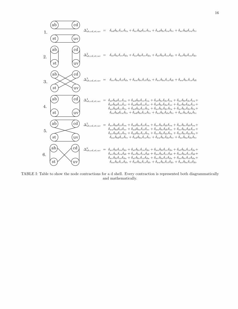
The terms in Eq. (B8) that can generate a rank 0 (ascalar) are 0⊗ 0, 1⊗ 1, 2⊗ 2, 3⊗ 3 and 4⊗ 4. This im-plies that a general isotropic three-dimensional eighth-rank tensor is defined by five independent parameters.We know that, for Vαβ,χγ , there exists a symmetry be-tween the pairs αχ and βγ. It follows that Vab,cd,st,uv hasa symmetry between the pairs (ab)(st) and (cd)(uv). Wetherefore require only the even contractions, 0⊗ 0, 2⊗ 2and 4 ⊗ 4, reducing the five parameters to three45; thisis the same number proposed in Chapter 4 of Ref. 35.To get the scalars from Vab,cd,st,uv we have to contractit. There are six possible contractions of Vab,cd,st,uv, out-lined in Table I, of which only five are independent. Notethat one does not contract within the indices ab, cd, st oruv because Bab is traceless, hence

∑ab δabBab = 0. By

examining the diagrammatic contractions from Table I,and maintaining the symmetry between the pairs (ab)(st)and (cd)(uv), we conclude that the relevant contractions

are ∆2ab,cd,st,uv,

(∆1ab,cd,st,uv + ∆3

ab,cd,st,uv

), ∆5

ab,cd,st,uv

and(

∆4ab,cd,st,uv + ∆6

ab,cd,st,uv

). This is evident because

switching two symmetry-related pairs [that is, switching(ab) and (st) or (cd) and (su)] in diagram 1 yields dia-gram 3. Similarly, switching two symmetry-related pairsin diagram 4 yields diagram 6. We see that there are fourcontractions but we have only three parameters. Thisimplies that out of these four contractions there are onlythree linearly independent contractions.We can now write down a general interaction Hamilto-nian Vab,cd,st,uv as a linear combination of three Kro-

necker delta products, each multiplied by one of the threeindependent coefficients:

Vab,cd,st,uv = c0∆2ab,cd,st,uv

+ c1(∆1ab,cd,st,uv + ∆3

ab,cd,st,uv

)+ c2∆5

ab,cd,st,uv. (B9)

We find Vαβ,χγ by transforming this expression back tothe five-dimensional fourth-rank representation, as dic-tated by Eq. (B7). For completeness we include all six ofthe transformed contractions:∑

abcd

∑stuv

∆1ab,cd,st,uvξαabξβcdξχstξγuv =∑

abst

4ξαabξβbaξχstξγts = δαβδχγ ,∑abcd

∑stuv

∆2ab,cd,st,uvξαabξβcdξχstξγuv =∑

abcd

4ξαabξχbaξβcdξγdc = δαχδβγ ,∑abcd

∑stuv

∆3ab,cd,st,uvξαabξβcdξχstξγuv =∑

abcd

4ξαabξγbaξβcdξχdc = δαγδβχ,∑abcd

∑stuv

∆4ab,cd,st,uvξαabξβcdξχstξγuv =∑

abdv

16ξαabξβbdξγdvξχva,∑abcd

∑stuv

∆5ab,cd,st,uvξαabξβcdξχstξγuv =∑

abdt

16ξαabξβbdξχdtξγta,∑abcd

∑stuv

∆6ab,cd,st,uvξαabξβcdξχstξγuv =∑

abdt

16ξαabξχbtξβtdξγda. (B10)

We find that the last three of the transformations ofthe contractions, although rotationally invariant in or-bital space, are not expressible in terms of Kroneckerdeltas of α, β, χ and γ. This is to be expected asthere exist terms in Vαβ,χγ that are non-zero and havemore than two orbital indices, e.g. V(3z2−r2)(xy),(yz)(xz)

or V(3z2−r2)(xy),(xy)(x2−y2).We can now write down Vαβ,χγ concisely,

Vαβ,χγ = Uδαχδβγ +

(J +

5

2∆J

)(δαγδβχ + δαβδχγ)

− 48∆J∑abdt

ξαabξβbdξχdtξγta, (B11)

where we have defined U to be the Hartree termbetween the t2g orbitals on-site, U = V(zx)(yz),(zx)(yz),J to be the average of the exchange integral

13

between the eg and t2g orbitals on-site, J =12

(V(zx)(yz),(yz)(zx) + V(3z2−r2)(x2−y2),(x2−y2)(3z2−r2)

),

and ∆J to be the difference between theexchange integrals for eg and t2g, ∆J =V(3z2−r2)(x2−y2),(x2−y2)(3z2−r2) − V(zx)(yz),(yz)(zx).We could equally well have chosen to use the sum ofthe fourth and sixth contractions instead of the fifthcontraction, although with different coefficients.

Appendix C: Angular momentum and quadrupoleoperators

1. Angular momentum

The angular momentum operators are most naturally ex-pressed in spherical polar coordinates, even when usingthem to operate on cubic harmonics. Their forms are:

Lx = i

(sinφ

∂

∂θ+ cot θ cosφ

∂

∂φ

), (C1)

Ly = i

(− cosφ

∂

∂θ+ cot θ sinφ

∂

∂φ

), (C2)

Lz = −i ∂∂φ, (C3)

where we have set h to 1 for simplicity. When applyingthe above operators to the on-site cubic harmonic p or-bitals (we have dropped the site index for clarity) it isstraightforward to show that

Lµpj = i∑k

εµjkpk. (C4)

A general one particle operator O may be expressed interms of creation and annihilation operators as follows:

O =∑αβσσ′

〈φασ|O|φβσ′〉c†ασ cβσ′ . (C5)

Substituting Eq. (C4) into Eq. (C5) yields

Lµ = i∑αβσ

εµβαc†ασ cβσ, (C6)

where µ is a Cartesian direction and α and β are cubicharmonic p orbitals (x, y or z). The d case is slightlymore complicated, but is greatly simplified by the use ofEq. (B6). Applying the angular momentum operators tothe B matrix reveals that

Lµ|Bjk〉 = i∑s

(εµjs|Bsk〉+ εµks|Bjs〉) , (C7)

with

Lµ|φασ〉 = iNd∑jks

S(σ)Rd(r)

r2ξαjk (εµjs|Bsk〉+ εµks|Bjs〉) .

(C8)

By finding the expectation value and substituting intoEq. (C5) we obtain

Lµ = 4i∑jkm

∑αβσ

εµmkξαkjξβjmc†ασ cβσ. (C9)

2. Quadrupole operator

We define the quadrupole operator for a single electronas

Qµν =1

2

(LµLν + LνLµ

)− 1

3δµνL

2. (C10)

Here we interpret Lµ and Lν in Eq. (C10) as compo-nents of the angular momentum of a single electron.The quadrupole operator for a system of N electronsis then a sum over contributions from each electron:Qµν =

∑Ni=1 Qµν(i). This makes Qµν a one-electron

operator, respresented in second quantization as a lin-ear combination of strings of one creation operator andone annihilation operator. Squaring and tracing the one-electron tensor operator Qµν yields a two-electron oper-

ator Q2 =∑µν QµνQνµ.

To find the form of this operator, we start by applying thesingle electron version of Qµν to the B matrix, making

use of Eq. (C7). Starting with LµLν

LµLν |Bjk〉 = iLµ∑s

(ενjs|Bsk〉+ ενks|Bjs〉) ,

= (i)2∑ss′

(ενjs (εµss′ |Bs′k〉+ εµks′ |Bss′〉)

+ ενks (εµjs′ |Bs′s〉+ εµss′ |Bjs′〉)),

= (−1)

(δjµ|Bνk〉+ δkµ|Bjν〉 − 2δνµ|Bjk〉

+∑ss′

(ενjsεµks′ + ενksεµjs′) |Bss′〉), (C11)

LνLµ|Bjk〉 = (−1)

(δjν |Bµk〉+ δkν |Bjµ〉 − 2δµν |Bjk〉

+∑ss′

(εµjsενks′ + εµksενjs′) |Bss′〉), (C12)

where the last equation was found by exchanging µ andν in the previous equation. Following the same process,the final term in Eq. (C10) becomes∑

ν

LνLν |Bjk〉 = 6|Bjk〉, (C13)

This is not a surprising result as the B matrix containslinear combinations of spherical harmonics |l, lz〉 with l =

2, and L2|l, lz〉 = l(l + 1)|l, lz〉. Combining Eqs. (C11),

14

(C12) and (C13) we find

Qµν |Bjk〉 = −(

1

2(δµj |Bνk〉+ δkµ|Bjν〉

+δjν |Bµk〉+ δkν |Bjµ〉)

+∑ss′

(ενjsεµks′ + ενksεµjs′) |Bss′〉). (C14)

Equation (C5) yields the corresponding operator for asystem of many electrons:

Qµν = −∑αβσ

(2∑k

(ξανkξβkµ + ξαµkξβkν

)+ 4

∑mnjk

ξαmnξβjkενjmεµkn

)c†ασ cβσ. (C15)

We now define the normal ordered quadrupole squaredas

: Q2 :=∑µν

: QµνQνµ : . (C16)

By substituting Eq. (C15) into Eq. (C16) and droppingthe site index for clarity, one obtains the following simpleformula for the quadrupole squared operator:

: Q2 : =∑

αβγχσσ′

(− 3δαχδβγ + 9

(δαγδβχ + δαβδχγ

)− 72

∑stuv

ξαstξβtuξχuvξγvs

)c†ασ c

†βσ′ cγσ′ cχσ. (C17)

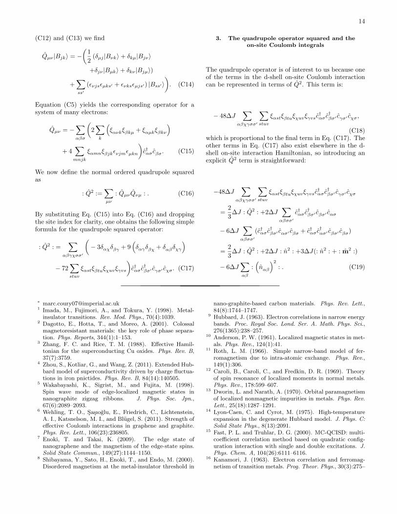
3. The quadrupole operator squared and theon-site Coulomb integrals

The quadrupole operator is of interest to us because oneof the terms in the d-shell on-site Coulomb interactioncan be represented in terms of Q2. This term is:

− 48∆J∑

αβχγσσ′

∑stuv

ξαstξβtuξχuvξγvsc†ασ c†βσ′ cγσ′ cχσ,

(C18)which is proportional to the final term in Eq. (C17). Theother terms in Eq. (C17) also exist elsewhere in the d-shell on-site interaction Hamiltonian, so introducing anexplicit Q2 term is straightforward:

−48∆J∑

αβχγσσ′

∑stuv

ξαstξβtuξχuvξγvsc†ασ c†βσ′ cγσ′ cχσ

=2

3∆J : Q2 : +2∆J

∑αβσσ′

c†ασ c†βσ′ cβσ′ cασ

− 6∆J∑αβσσ′

(c†ασ c†βσ′ cασ′ cβσ + c†ασ c

†ασ′ cβσ′ cβσ)

=2

3∆J : Q2 : +2∆J : n2 : +3∆J(: n2 : + : m2 :)

− 6∆J∑αβ

:(nαβ

)2: . (C19)

∗ marc.coury07@imperial.ac.uk1 Imada, M., Fujimori, A., and Tokura, Y. (1998). Metal-

insulator transitions. Rev. Mod. Phys., 70(4):1039.2 Dagotto, E., Hotta, T., and Moreo, A. (2001). Colossal

magnetoresistant materials: the key role of phase separa-tion. Phys. Reports, 344(1):1–153.

3 Zhang, F. C. and Rice, T. M. (1988). Effective Hamil-tonian for the superconducting Cu oxides. Phys. Rev. B,37(7):3759.

4 Zhou, S., Kotliar, G., and Wang, Z. (2011). Extended Hub-bard model of superconductivity driven by charge fluctua-tions in iron pnictides. Phys. Rev. B, 84(14):140505.

5 Wakabayashi, K., Sigrist, M., and Fujita, M. (1998).Spin wave mode of edge-localized magnetic states innanographite zigzag ribbons. J. Phys. Soc. Jpn.,67(6):2089–2093.

6 Wehling, T. O., Sasıoglu, E., Friedrich, C., Lichtenstein,A. I., Katsnelson, M. I., and Blugel, S. (2011). Strength ofeffective Coulomb interactions in graphene and graphite.Phys. Rev. Lett., 106(23):236805.

7 Enoki, T. and Takai, K. (2009). The edge state ofnanographene and the magnetism of the edge-state spins.Solid State Commun., 149(27):1144–1150.

8 Shibayama, Y., Sato, H., Enoki, T., and Endo, M. (2000).Disordered magnetism at the metal-insulator threshold in

nano-graphite-based carbon materials. Phys. Rev. Lett.,84(8):1744–1747.

9 Hubbard, J. (1963). Electron correlations in narrow energybands. Proc. Royal Soc. Lond. Ser. A. Math. Phys. Sci.,276(1365):238–257.

10 Anderson, P. W. (1961). Localized magnetic states in met-als. Phys. Rev., 124(1):41.

11 Roth, L. M. (1966). Simple narrow-band model of fer-romagnetism due to intra-atomic exchange. Phys. Rev.,149(1):306.

12 Caroli, B., Caroli, C., and Fredkin, D. R. (1969). Theoryof spin resonance of localized moments in normal metals.Phys. Rev., 178:599–607.

13 Dworin, L. and Narath, A. (1970). Orbital paramagnetismof localized nonmagnetic impurities in metals. Phys. Rev.Lett., 25(18):1287–1291.

14 Lyon-Caen, C. and Cyrot, M. (1975). High-temperatureexpansion in the degenerate Hubbard model. J. Phys. C:Solid State Phys., 8(13):2091.

15 Fast, P. L. and Truhlar, D. G. (2000). MC-QCISD: multi-coefficient correlation method based on quadratic config-uration interaction with single and double excitations. J.Phys. Chem. A, 104(26):6111–6116.

16 Kanamori, J. (1963). Electron correlation and ferromag-netism of transition metals. Prog. Theor. Phys., 30(3):275–

15

289.17 Maitra, N. T., Zhang, F., Cave, R. J., and Burke, K.

(2004). Double excitations within time-dependent den-sity functional theory linear response. J. Chem. Phys.,120:5932.

18 Moszynski, R., Jeziorski, B., and Szalewicz, K. (1994).Many-body theory of exchange effects in intermolecularinteractions. Second-quantization approach and compari-son with full configuration interaction results. J. Chem.Phys., 100:1312.

19 Castellani, C., Natoli, C. R., and Ranninger, J. (1978).Magnetic structure of V2O3 in the insulating phase. Phys.Rev. B, 18(9):4945.

20 In this notation t2g refers to cubic harmonic d orbitalsdxy, dyz and dxz and eg refers to cubic harmonic d orbitalsd3z2−r2 and dx2−y2 .

21 Oles, A. M. and Stollhoff, G. (1984). Correlation effectsin ferromagnetism of transition metals. Phys. Rev. B,29(1):314.

22 Nolting, W., Borgiel, W., Dose, V., and Fauster, Th.(1989). Finite-temperature ferromagnetism of nickel. Phys.Rev. B, 40(7):5015.

23 Desjonqueres, M.-C., Barreteau, C., Autes, G., and Span-jaard, D. (2007). Orbital contribution to the magneticproperties of iron as a function of dimensionality. Phys.Rev. B, 76(2):024412.

24 Dudarev, S. L. and Derlet, P. M. (2007). Interatomic po-tentials for materials with interacting electrons. J. Com-put. Mater. Des., 14(1):129–140.

25 Nguyen-Manh, D. and Dudarev, S. L. (2009). Model many-body Stoner Hamiltonian for binary FeCr alloys. Phys.Rev. B, 80(10):104440.

26 Condon, E. U. (1930). The theory of complex spectra.Phys. Rev., 36:1121–1133.

27 Slater, J. C. (1929). The theory of complex spectra. Phys.Rev., 34(10):1293.

28 Gaunt, J. A. (1929). The triplets of helium. Philos. Trans-actions Royal Soc. Lond. Ser. A, Containing Pap. Math.or Phys. Character, pages 151–196.

29 Racah, G. (1942). Theory of complex spectra. II. Phys.Rev., 62(9-10):438.

30 Powell, R. C. (1998). Physics of solid-state laser materials,volume 1. Springer Science & Business Media. Pages 45–

48.31 Rudzikas, Z. B. (1997). Theoretical atomic spectroscopy.

Cambridge University Press (Cambridge and New York).32 Spencer, J. S., Thom, A. J. W., Blunt, N. S., Vigor, W. A.,

Malone, F. D., Shepherd, J. J., Foulkes, W. M. C., Rogers,T. W., Handley, W., and Weston, J. (2015). HANDE quan-tum Monte Carlo. http://www.hande.org.uk/.

33 Helgaker, T., Jørgensen, P., Olsen, J., and Ratner, M. A.(2001). Molecular electronic-structure theory. Phys. To-day, 54:52.

34 Matthews, P. C. (2000). Vector calculus. Springer.35 Griffith, J. S. (1961). The theory of transition-metal ions.

Cambridge University Press.36 Kosevich, A. M. (2005). The Crystal Lattice: Phonons,

Solitons, Dislocations. Wiley-VCH Weinheim.37 Sakai, S. (2006). Theoretical study of multi-orbital corre-

lated electron systems with Hunds coupling. PhD thesis,Univ. Tokyo.

38 Stollhoff, G., Oles, A. M., and Heine, V. (1990). Stonerexchange interaction in transition metals. Phys. Rev. B,41(10):7028.

39 Andersen, O. K. (1975). Linear methods in band theory.Phys. Rev. B, 12(8):3060.

40 Paxton, A. T. and Finnis, M. W. (2008). Magnetic tightbinding and the iron-chromium enthalpy anomaly. Phys.Rev. B, 77:024428.

41 Landau, L. D. and Lifshitz, E. M. (1981). Quantum me-chanics non-relativistic theory, volume 3. Butterworth-Heinemann.

42 Flensberg, H. B. K. and Bruus, H. (2004). Many-BodyQuantum Theory in Condensed Matter Physics. OxfordUniversity Press New York.

43 Fulton, W. and Harris, J. (1991). Representation theory:a first course, volume 129. Springer.

44 Kearsley, E. A. and Fong, J. T. (1975). Linearly inde-pendent sets of isotropic Cartesian tensors of ranks up toeight. J. Res. Natl Bureau Standards Part B: Math. Sci.B, 79:49–58.

45 By continuing this argument, one finds that there 4 pa-rameters are required to describe the on-site Coulomb in-teractions for an f shell (arising from 0 ⊗ 0, 2 ⊗ 2, 4 ⊗ 4and 6 ⊗ 6) and 5 parameters for a g shell (arising from0⊗0, 2⊗2, 4⊗4, 6⊗6 and 8⊗8), respectively. This trendcontinues with increasing angular momentum.

16

1.

3.

2.

4.

5. 6.

ab

st uv

cd ab

st uv

cd

ab

st uv

cd ab

st uv

cd

ab

st uv

cd ab

st uv

cd

∆1ab,cd,st,uv = δadδbcδsvδtu + δacδbdδsvδtu + δadδbcδsuδtv + δacδbdδsuδtv

1.

3.

2.

4.

5. 6.

ab

st uv

cd ab

st uv

cd

ab

st uv

cd ab

st uv

cd

ab

st uv

cd ab

st uv

cd

∆2ab,cd,st,uv = δatδbsδcvδdu + δasδbtδcvδdu + δatδbsδcuδdv + δasδbtδcuδdv

1.

3.

2.

4.

5. 6.

ab

st uv

cd ab

st uv

cd

ab

st uv

cd ab

st uv

cd

ab

st uv

cd ab

st uv

cd

∆3ab,cd,st,uv = δavδbuδctδds + δauδbvδctδds + δavδbuδcsδdt + δauδbvδcsδdt

1.

3.

2.

4.

5. 6.

ab

st uv

cd ab

st uv

cd

ab

st uv

cd ab

st uv

cd

ab

st uv

cd ab

st uv

cd

∆4ab,cd,st,uv = δatδbdδcvδsu + δadδbtδcvδsu + δatδbcδdvδsu + δacδbtδdvδsu+

δatδbdδcuδsv + δadδbtδcuδsv + δatδbcδduδsv + δacδbtδduδsv+δasδbdδcvδtu + δadδbsδcvδtu + δasδbcδdvδtu + δacδbsδdvδtu+δasδbdδcuδtv + δadδbsδcuδtv + δasδbcδduδtv + δacδbsδduδtv

1.

3.

2.

4.

5. 6.

ab

st uv

cd ab

st uv

cd

ab

st uv

cd ab

st uv

cd

ab

st uv

cd ab

st uv

cd∆5ab,cd,st,uv = δavδbdδctδsu + δadδbvδctδsu + δavδbcδdtδsu + δacδbvδdtδsu+

δauδbdδctδsv + δadδbuδctδsv + δauδbcδdtδsv + δacδbuδdtδsv+δavδbdδcsδtu + δadδbvδcsδtu + δavδbcδdsδtu + δacδbvδdsδtu+δauδbdδcsδtv + δadδbuδcsδtv + δauδbcδdsδtv + δacδbuδdsδtv

1.

3.

2.

4.

5. 6.

ab

st uv

cd ab

st uv

cd

ab

st uv

cd ab

st uv

cd

ab

st uv

cd ab

st uv

cd ∆6ab,cd,st,uv = δavδbtδcuδds + δatδbvδcuδds + δauδbtδcvδds + δatδbuδcvδds+

δavδbsδcuδdt + δasδbvδcuδdt + δauδbsδcvδdt + δasδbuδcvδdt+δavδbtδcsδdu + δatδbvδcsδdu + δavδbsδctδdu + δasδbvδctδdu+δauδbtδcsδdv + δatδbuδcsδdv + δauδbsδctδdv + δasδbuδctδdv

TABLE I: Table to show the node contractions for a d shell. Every contraction is represented both diagrammaticallyand mathematically.