Huber-Norm Regularization for LinearPrediction Models

Oleksandr Zadorozhnyi1, Gunthard Benecke1, Stephan Mandt2,Tobias Scheffer1, Marius Kloft3

1 University of Potsdam, Department of Computer Science{zadorozh, gunthard.benecke, tobias.scheffer}@uni-potsdam.de

2 Columbia University, Data Science Institute, Department of Computer Sciencesm3976@columbia.edu

3 Humboldt-Universitat zu Berlin, Department of Computer Sciencekloft@hu-berlin.de

Abstract. In order to avoid overfitting, it is common practice to reg-ularize linear prediction models using squared or absolute-value normsof the model parameters. In our article we consider a new method ofregularization: Huber-norm regularization imposes a combination of `1and `2-norm regularization on the model parameters. We derive the dualoptimization problem, prove an upper bound on the statistical risk ofthe model class by means of the Rademacher complexity and establisha simple type of oracle inequality on the optimality of the decision rule.Empirically, we observe that logistic regression with Huber-norm regu-larizer outperforms `1-norm, `2-norm, and elastic-net regularization fora wide range of benchmark data sets.

1 Introduction

Linear classification and regression models—such as the support vector machine(SVM) and logistic and linear regression—are widely used in machine learning,and regularized empirical-risk minimization is a standard approach to optimizingtheir parameters. To avoid overfitting, linear models are typically either denselyor sparsely regularized. With an `2 regularizer, one obtains a dense weight vectorin which all features contribute to the prediction task. For interpretability, oneis often interested in a sparse solution in which many entries of the weight vectorare zero. To this end, one may employ an `1 absolute value norm regularizer [25,18]. While this type of regularization may lead to lower predictive accuraciesthan `2 regularization [10], the result focuses only on the most relevant features.

This paper promotes the idea of using a combination of both types of regu-larization, thus combining the best of both worlds. Instead of using just a singleweight vector w that is either dense or sparse, we employ a sum of two weightvectors w+v. While w is `2 regularized and therefore dense, v is `1 regularizedand therefore sparse. Having two different weight vectors with different regular-izations allows linear models to more flexibly fit the data. It comes at a moderatecomputational cost, since the number of parameters is doubled.

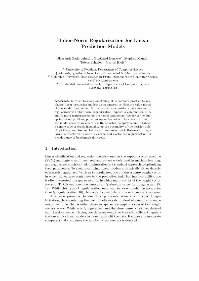
Fig. 1. Geometrical illustration of the proposed Huber-norm regularizer and compari-son to common regularizers.

We first show that the proposed combination of two weight vectors is mathe-matically equivalent to imposing Huber-norm [7] regularization on the empiricalrisk of a linear model. This approach is known to be statistically more robust [8]in the sense that individual sparse weights do not necessarily involve a huge costin the loss. This Huber norm involves quadratic costs near the origin and linearcosts far away from the origin, this way penalizing outliers less severely. Becauseof this analogy, we call our method Huber-norm regularization. We derive uni-form and data-dependent upper bounds on the statistical risk of the model classby means of the Rademacher complexity. We deduce a simple type of oracleinequality on the inference efficiency of the decision rule which measures thedeviation of the model’s risk from the lowest risk of any model in the class.

Our empirical studies show that Huber-norm regularized logistic regressionoutperforms `1- and `2-regularized as well as elastic-net-regularized logistic re-gression [26] in the majority of cases over a wide range of benchmark problems.To support this claim we provide evidence based on empirical studies on theUCI machine learning repository, where our method performs best among thecompared methods on 23 out of 31 data sets. On particular data set—the well-known Iris data set—Huber-norm regularization leads to a prediction accuracyof 0.96 while the next-best method merely achieves 0.84.

Our paper is organized as follows. Section 2 reviews related work. In Section 3,we describe our model and its basic properties. We also prove the equivalenceof the two weight vectors to Huber-norm regularization in the conventional set-ting. In Section 4 we then present the underlying theoretical foundations of ourapproach, where we prove an upper bound on the statistical risk. We presentour experimental results in section 5 and conclude in Section 6.

2 Related Work

Comparisons between `1-norm and `2-norm SVMs are ubiquitous in the liter-ature [25, 14, 13]. A robust alternative to the SVM based on the smooth ramploss [23] requires the convex-concave procedure to convert this non-convex op-timization problem into a convex one [24]. Another way of making the SVMrobust [20] is based on the weighted LS-SVM that yields sparse results. Differ-

2

ent type of classification problems for the SVM (both convex and non-convex)are discussed by Hailong et al. [6] where the conjugate gradient approach is usedto solve the optimization problem.

Our novel type of regularizer relates to the elastic-net regularizer [26] thatsimply amounts to taking the sum of an `1 and `2 regularizer. Our proposedregularizer is very different, as is evident from Figure 1. The plot shows contoursof different regularizers in comparison. As a major difference between the elasticnet and our approach, our regularizer grows asymptotically linearly for largeweight vectors whereas the elastic net grows asymptotically quadratically. Lastly,our theoretical contributions are based on fundamental work by Vapnik [22].

The Huber norm [7] is frequently used as a loss function; it penalizes outliersasymptotically linearly which makes it more robust than the squared loss. TheHuber norm is used as a regularization term of optimization problems in imagesuper resolution [21] and other computer-graphics problems. The inverse Huberfunction [17] has been studied as a regularizer for regression problems. While theHuber norm penalizes large weights asymptotically linearly, the inverse Huberfunction imposes an asymptotically squared penalty on large weights.

3 Huber-Norm-Regularized Linear Models

In this section, after formally introducing the problem setting and optimizationcriterion, we show that this optimization criterion has an equivalent formulationin which the Huber norm becomes explicit. We derive the dual form and showhow Huber-norm regularization for linear models can be implemented.

3.1 Problem Setting and Preliminaries

We consider the standard supervised prediction setup, where we are given atraining sample S = {xi, yi}ni=1 from a space X × Y with X = Rd. We aimat finding a linear function f that predicts well. A common way to achievethis is to first define a loss function ` : R × Y → R+ ∪ {0} that measures thedeviation of the prediction f(x) from the correct value y, such as the logistic loss`(f(x), y) := log(1 + exp(−yf(x))) or hinge loss `(f(x), y) := max(0, 1− yf(x)).The empirical risk is then the averaged loss over the training sample, Ln(f) =1n

∑ni=1 `(f(xi), yi) of f .

In this paper we consider methods that employ linear prediction functionsf(x) = w>x. To avoid overfitting, one usually uses a regularizer such as the `1regularizer R1(w) = ‖w‖1, the `2 regularizer R2(w) = ‖w‖22, or the elastic-net

regularizer Ren(w) = ‖w‖1 +‖w‖22. This results in the regularized empirical riskminimization or short reg-ERM problem:

minw

λR(w) +1

n

n∑i=1

`(yi,w>xi).

The `1 and elastic-net regularizers produce sparse, `2-norm regularizer denseweight vectors. Hence, depending on the problem, the regularizer can be chosento match the underlying sparsity of the problem.

3

3.2 Linear Models with Sums of Dense and Sparse Weights

Using `1-, `2-, or elastic-net-regularized ERM either produces dense or sparsesolutions. In this paper, we argue it can be beneficial to produce dense solutionswith pronounced feature weights as in `1-norm regularized methods. We pro-pose to consider linear models of the form f(x) := (v + w)>x (for notationalconvenience, we disregard constant offsets and assume that the first element ofeach x is a constant 1) and the regularizer RH(v,w) = λ ‖v‖1 + µ ‖w‖22, henceresulting in the following optimization problem.

Optimization Problem 1 (Sums of dense and sparse weights) Givenλ, µ > 0 and loss function `(t, y), solve:

(w, v) = arg minv,w

G(w,v, S)

with G(w,v, S) = λ||v||1 + µ ‖w‖22 +1

n

n∑i=1

`(yi, (w + v)>xi), (1)

where || · ||2 and || · ||1 denote standard `2-norm and `1-norm correspondingly.

For reasons that will become clear in the section below we call the method Huber-regularized empirical risk minimization or short Huber-regERM. Note that byletting λ→∞, we obtain the classic `2-norm regularization, while letting µ→∞leads to `1-norm regularization. Thus these methods are obtained as limit casesof our method. Elastic-net-regularization is not a special case of this framework,but it could be obtained by enforcing an additional constraint v = w.

3.3 Geometry of the Huber Norm

The following geometrical interpretation lets us compare linear models with sumsof dense and sparse weights to the `1, `2, and elastic-net regularizers. We provethat Problem 1 is equivalent to the following problem.

Optimization Problem 2 (Equivalent Huber-Norm Problem)Optimization Problem 1 can equivalently be formulated as:

z = arg minz

RH(z) +1

n

n∑i=1

`(yi, z>xi) (2)

where RH(z) =∑di=1 rH(zi), and rH(zi) =

{λ(|zi| − λ

4µ

)if |zi| ≥ λ

2µ

µz2i , otherwise.

Note that RH(z) is the Huber norm of z. While the Huber norm is often used asa robust loss function that is less sensitive to outliers, Optimization Problem 2employs the Huber norm as regularizer. Intuitively, this results in a regularizationscheme that is less sensitive to individual features which have a stong impact on

4

f than `2 regularization. Figure 1 illustrates isotropic lines for the Huber-normregularizer and known regularizers for λ = µ = 1. The Huber norm is composedof linear and squared segments. While it does not encourage sparsity as the `1regularizer does, it encourages that most attributes only have a small impact onthe decision function.

Proof (Equivalence of Optimization Problems 1 and 2). Let z = w+v. Problem 1can then be formulated as

minw,v

G(w,v, S) = minz,v

λ||v||1 + µ ‖z− v‖22 +1

n

n∑i=1

`(yi, z>xi)

= minz

(µmin

v

(λ

µ||v||1 + ‖z− v‖22

)+

1

n

n∑i=1

`(yi, z>xi)

). (3)

Let us define R(v, z) := c||v||1 + ‖z− v‖22 where c := λµ . It remains to be shown

that minvR(v, z) is a Huber-norm regularizer.

Simplifying R = v>v − 2v>(z− c

2 sgn(v))

+ z>z, we find

minvR = min

v(v1,...,vd)

(d∑i=1

v2i − 2vi(zi −c

2sgn(vi))

)+

d∑i=1

z2i . (4)

For each i ∈ {1, ..., d} we minimize Ri := v2i − 2vi(zi− c2 sgn(vi)) with respect to

vi. This is equivalent to:minvi

v2i − 2(zi − c2 )vi if vi > 0

minvi

v2i − 2(zi + c2 )vi if vi ≤ 0.

We can minimize each of these two quadratic terms analytically:[−(zi − c

2 )2 if zi ∈ A := {z ∈ R : |z| ≥ c2}

0 if zi ∈ Ac := {z ∈ R : |z| < c2}.

This means, that for Equation 4 we have explicitly:

minvR =

d∑i=1

(z2i −

(zi −

c

2

)2

Izi∈A

)=

d∑i=1

(z2i Izi∈AC + c

(|zi| −

c

4

)Izi∈A

).

This is exactly the Huber-norm regularizer RH(z) of Optimization Problem 2.ut

3.4 Dual Problem

In order to classify a training point, we need to compute the scalar product(w+v)>x which may be expensive when the dimension of vectors w,v is large.

5

One possible solution to overcome this consists in considering a weighted sum ofconstraints together with an objective function computed on the training sample.This leads to a dual approach. Steinwart [19] gives a general overview of dualoptimization problems for SVMs using `2- and `1-norm regularizers. The dualform of the optimization problem depends on the loss function. We completeSteinwart’s overview by deriving the dual form of the Huber-norm regularizedSVM in the following.

Optimization Problem 3 (Dual Huber-Norm SVM Problem)Optimization Problem 1 with hinge-loss loss function (Huber-Norm SVM)has an equivalent dual form which can be formulated as follows:

maxα∈Rn

n∑i=1

αi −1

2

n∑i,j=1

αiαjyiyjx>i xj

s.t. α ∈ [0, C]n ∧ ||X>α||∞ ≤λ

2µ, (5)

where C := 12nµ and X = (x1, ...,xn) ∈ Rn×d.

Proof. The Lagrangian L(w,v, ξ, α, η) that corresponds to Equation 1 is givenas follows:

L(w,v, ξ, α, η) := C

n∑i=1

ξi +λ

2µ||v||1 +

1

2||w||22+

n∑i=1

αi(1− yi(w> + v>)xi − ξi

)−

n∑i=1

ηiξi, (6)

where α = (α1, ..., αn) ∈ [0,∞)n and η = (η1, ..., ηn) ∈ [0,∞)n. So the dualproblem [3] can be written as:

maxα,η

infw,v,ξ

L(w,v, ξ, α, η). (7)

Grouping the terms in the Lagrangian gives us:

L(w,v, ξ, α, η) =

n∑i=1

(C − αi − ηi)ξi +λ

2µ||v||1

−n∑i=1

αiyiv>xi +

1

2||w||22 −

n∑i=1

αiyiw>xi +

n∑i=1

αi.

Now, considering the infimum with respect to v and w separately, and using thedefinition of a conjugate function [3, 19] we obtain:

infv

λ

2µ||v||1 −

n∑i=1

αiyiv>xi = − sup

v

λ

2µ||v||1 + v>

n∑i=1

αiyixi

=

{0, when |X>α||∞ ≤ λ

2µ

−∞, otherwise,(8)

6

where X = (x1, ...,xn) ∈ Rn×d is the data matrix whose rows x>i are the in-stances and ‖·‖∞ -supremum norm in Rd. Analogously, for w we have:

infw

1

2||w||22 −

n∑i=1

αiyiw>xi = − sup

w−1

2||w||22 + w>

n∑i=1

αiyixi

=1

2

(n∑i=1

αiyixi

)>( n∑i=1

αiyixi

). (9)

Finally, computing the gradient with respect to ξ gives that for each i ∈ {1, ...n}:

C − ηi − αi = 0⇔ αi = C − ηi. (10)

Now, for fixed λ, µ, and X, define P = {α|α ∈ [0, C]n ∧ ||X>α||∞ ≤ λ2µ},where

y = (y1, ..., yn) ∈ Rn. Substituting Equations 8, 9, and 10 into Equation 7 givesthe following dual problem:

maxα∈P

n∑i=1

αi −1

2

n∑i,j=1

αiαjyiyjx>i xj , (11)

which is a quadratic optimization problem within set P and can be solved withknown methods.

ut

By close inspection of Equation 11, we observe that our dual optimizationproblem closely resembles the one for SVM using `2 regularization, but with adifference in the form of the domain P of the optimization problem.

3.5 Algorithm & Implementation

Algorithm 1 implements Huber-regularized empirical risk minimization for linearmodels. The algorithm works by alternatingly minimizing the occurring `1-normand `2-norm regularized minimization problems, respectively. For each step ofoptimization procedure we use gradient descent, assuming that the other vectoris constant. The gradient of the `1 norm of v is not defined for v = 0; here, weuse subgradients [3].

4 Theoretical Analysis

In this section we present a theoretical analysis of the proposed Huber-normregularizer for linear models. We obtain bounds on the statistical risk based onthe established framework of Rademacher complexities [2, 16] and, consequently,on the norms of the vectors v,w and number of training samples n [2].

7

Algorithm 1 Optimization Procedure

1: Input: S = {xi, yi}ni=1

2: w = 0, v = 0.3: repeat4: solve w := arg min

wG(w,v, S) by gradient descent,

5: solve v := arg minv

G(w,v, S) by gradient descent,

6: let w,v = (w, v).7: until convergence.8: Output: w,v

4.1 Preliminaries and Aim

Let S = {xi, yi}ni=1 be a sample of n training points that are independentlydrawn from one and the same distribution PX,Y over X ×Y, where X = Rd; letthe output space Y be discrete for classification and continuous for regression.In this theoretical analysis, we study the Huber-regERM model class

F := {f : x 7→ (w + v)>x : Rd → R| ‖w‖2 ≤W, ‖v‖2 ≤ V }, (12)

where W and V are initially unknown constants. Loss function ` : R × Y →R+ ∪ {0} may be any convex loss function that is L-Lipschitz continuous andabsolutely bounded by constant B ∈ R. The aim of our theoretical analysis isto obtain bounds on the deviation of the risk L(f) = EPX,Y

[`(f(x), y)] of the

model f ∈ F from empirical risk Ln(f) = 1n

∑ni=1 `(f(xi), yi).

Let {σi}ni=1 be independent Rademacher random variables, meaning thateach of them is uniformly distributed over {−1,+1}. Denote by Σ the jointuniform distribution of σ1, . . . , σn. Then the empirical Rademacher complexityis defined as

RS(` ◦ F) := EΣ

[supf∈F

1

n

n∑i=1

σi`(f(xi), yi))

], (13)

and the (theoretical) Rademacher complexity [2, 16] is defined as Rn(` ◦ F) :=

ES [RS(`◦F)]. Here, the expectation is taken under the distribution of the sampleS. It has been shown [2, 16] that when ` is L-Lipschitz continuous in the secondargument, then with probability at least 1− δ, for all f ∈ F :

L(f) ≤ Ln(f) + 2LES[RS(F)

]+B

√log δ−1

2n. (14)

4.2 Bounds on the Risk of Huber-regularized Linear Models

Our main theoretical contributions are bounds on statistical risk based on data-dependent and uniform upper bounds on the Rademacher complexity of themodel class F defined by Equation 12.

8

Theorem 1 (Uniform risk bound for Huber regularization) Let F bedefined by Equation 12, let ` be a L-Lipschitz continuous loss function, andlet R be a constant such that |`(t, y)| ≤ R for all t ∈ R and y ∈ Y. Let the `2norm of all instances is bounded by ‖x‖2 ≤ Rx with probability 1 by some Rx.Then, for every δ ∈ (0, 1), with probability at least 1− δ the following holds forall f ∈ F :

L(f) ≤ Ln(f) + 2L√

2(W 2 + V 2)

nRx +R

√log δ−1

2n(15)

where W =√

Rµ , V = R

λ

Instead of relying on a uniform bound Rx on the data xi, we can give thefollowing data-dependent bound on the risk.

Proposition 1 (Data-dependent risk bound for Huber regularization)Let F be defined by Equation 12, and let ` be a L-Lipschitz continuous lossfunction. Then, for every δ ∈ (0, 1), with probability at least 1− δ the followingholds for all f ∈ F , where W , V , and R as defined as in Theorem 1:

L(f) ≤ Ln(f) + 2L

√2(W 2 + V 2)

n∑i=1

‖xi‖2

n+ (2L+ 1)R

√log( 2

δ )

2n. (16)

4.3 Lemmata and Auxilary Results

The risk bounds are based on the following three lemmas.

Lemma 1 For the functional class F of Equation 12, the following data-dependend bound on the empirical Rademacher complexity holds:

RS(F) ≤

√2(W 2 + V 2)

n∑i=1

‖xi‖2

n. (17)

Lemma 2 For the functional class F of Equation 12, the (theoretical)Rademacher complexity is bounded as follows:

Rn(F) = ES [RS(F)] ≤√

2(W 2 + V 2)

nRx. (18)

where Rx is a constant such that ||x||2 ≤ Rx almost surely under PX .

Lemma 3 Let (w, v) = arg minv,w

G(w,v, S). Then ‖w‖2≤√

Rµ , ‖v‖2≤

Rλ , where

R as in Theorem 1.

9

Proof (Lemma 1). Following the ideas presented by Mohri [16], we rewrite theempirical Rademacher complexity using the Cauchy-Schwartz inequality:

RS(F) =1

nEσ

[sup

‖w‖2≤W,‖v‖2≤V

n∑i=1

(σi(w + v)>xi

)]

=1

nEσ

[sup

‖w‖2≤W,‖v‖2≤V(w + v)>

n∑i=1

σixi

]

≤ 1

nEσ

[sup

‖w‖2≤W,‖v‖2≤V‖w + v‖2

∥∥∥∥∥n∑i=1

σixi

∥∥∥∥∥2

]. (19)

Using the inequality∑di=1(wi + vi)

2 ≤ 2∑di=1(w2

i + v2i ) for the right-handside of Equation 19, according to the restrictions on the norms of w,v we get:

Eσ

[sup

‖w‖2≤W,‖v‖2≤V‖w + v‖2

∥∥∥∥∥n∑i=1

σixi

∥∥∥∥∥2

]≤√

2(W 2 + V 2)Eσ

[∥∥∥∥∥n∑i=1

σixi

∥∥∥∥∥2

](20)

and because of Jensen’s inequality for Eσ [‖·‖], linearity of expectation and in-dependence of σi, σj for j 6= i we obtain:

Eσ

[∥∥∥∥∥n∑i=1

σixi

∥∥∥∥∥2

]≤

√√√√√Eσ

n∑i,j=1

σiσjxitxj

=

√√√√ n∑i=1

Eσ

[‖xi‖22

]=

√√√√ n∑i=1

‖xi‖22. (21)

Uniting the results of Inequality 20 and Equation 21 in Equation 19 we get thestatement of Lemma 1.

ut

Proof (Lemma 2). Using Lemma 1 and the assumption that the xi are uniformlybounded by constant Rx we obtain:

RS(F) ≤√

2(W 2 + V 2)

nRx. (22)

Equation 22 no longer depends on the sample, and therefore Lemma 2 follows.ut

Naturally, one may not have any a-priori knowledge about the constants Wand V that restrict the possible values of w and v in Inequality 18. Despite that,for a given optimization problem that includes the current class of models, onecan apply certain arguments from which one can infer bounds for W and V .Lemma 3 gives us such bounds for Optimization Problem 1.

10

Proof (Lemma 3). When (w, v) is a solution of optimization problem (1), then

G(w, v, S) ≤ G(0,0, S) ≤ R

This implies that the optimal solution necessarily satisfies the following condi-tion: λ ‖v‖1 + µ ‖w‖2 ≤ R. As far as ‖v‖1 ≥ ‖v‖2 we have that in order to bean optimal solution v should satisfy following constraint: ‖v‖2 ≤

Rλ . For w we

obtain straightforward necessary condition, that ‖w‖22 ≤Rµ which implies the

claim of Lemma 3.ut

Lemma 3 implies that the norms of the vectors v and w of a solution of

Optimization Problem 1 necessary have to lie within balls with radius W :=√

Rµ

for w and of radius V := Rλ for v, centered in the origin.

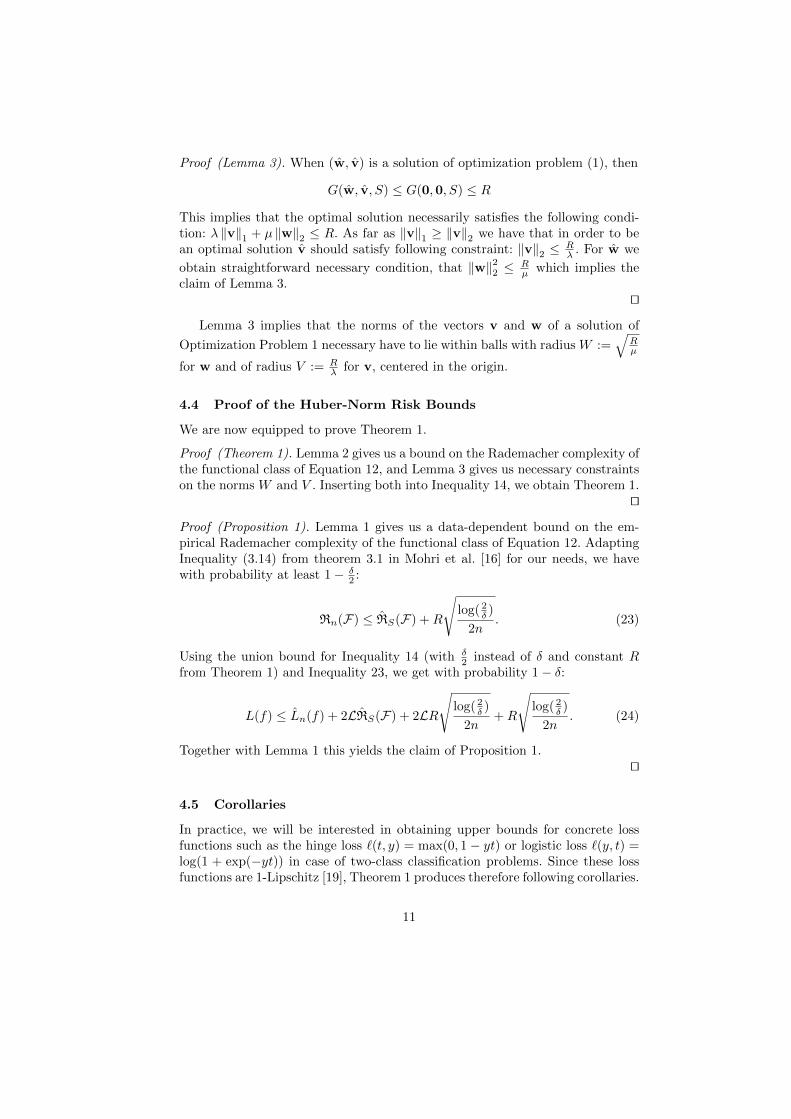
4.4 Proof of the Huber-Norm Risk Bounds

We are now equipped to prove Theorem 1.

Proof (Theorem 1). Lemma 2 gives us a bound on the Rademacher complexity ofthe functional class of Equation 12, and Lemma 3 gives us necessary constraintson the norms W and V . Inserting both into Inequality 14, we obtain Theorem 1.

ut

Proof (Proposition 1). Lemma 1 gives us a data-dependent bound on the em-pirical Rademacher complexity of the functional class of Equation 12. AdaptingInequality (3.14) from theorem 3.1 in Mohri et al. [16] for our needs, we havewith probability at least 1− δ

2 :

Rn(F) ≤ RS(F) +R

√log( 2

δ )

2n. (23)

Using the union bound for Inequality 14 (with δ2 instead of δ and constant R

from Theorem 1) and Inequality 23, we get with probability 1− δ:

L(f) ≤ Ln(f) + 2LRS(F) + 2LR

√log( 2

δ )

2n+R

√log( 2

δ )

2n. (24)

Together with Lemma 1 this yields the claim of Proposition 1.ut

4.5 Corollaries

In practice, we will be interested in obtaining upper bounds for concrete lossfunctions such as the hinge loss `(t, y) = max(0, 1− yt) or logistic loss `(y, t) =log(1 + exp(−yt)) in case of two-class classification problems. Since these lossfunctions are 1-Lipschitz [19], Theorem 1 produces therefore following corollaries.

11

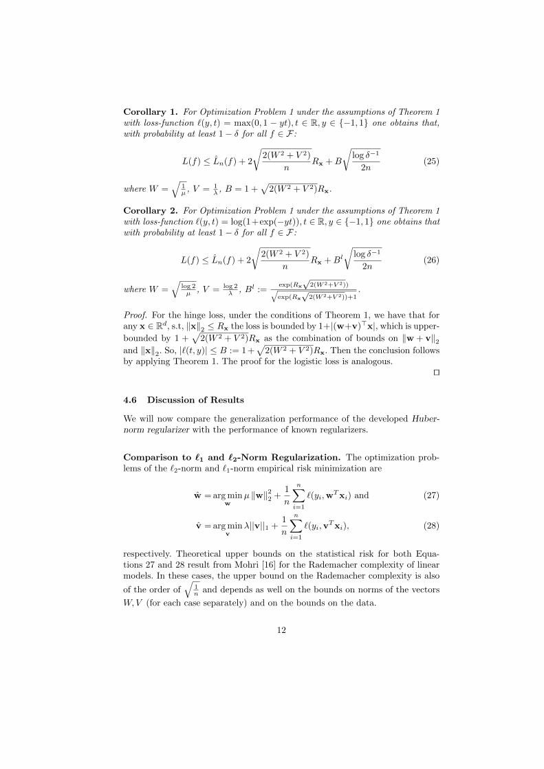
Corollary 1. For Optimization Problem 1 under the assumptions of Theorem 1with loss-function `(y, t) = max(0, 1 − yt), t ∈ R, y ∈ {−1, 1} one obtains that,with probability at least 1− δ for all f ∈ F :

L(f) ≤ Ln(f) + 2

√2(W 2 + V 2)

nRx +B

√log δ−1

2n(25)

where W =√

1µ , V = 1

λ , B = 1 +√

2(W 2 + V 2)Rx.

Corollary 2. For Optimization Problem 1 under the assumptions of Theorem 1with loss-function `(y, t) = log(1+exp(−yt)), t ∈ R, y ∈ {−1, 1} one obtains thatwith probability at least 1− δ for all f ∈ F :

L(f) ≤ Ln(f) + 2

√2(W 2 + V 2)

nRx +Bl

√log δ−1

2n(26)

where W =√

log 2µ , V = log 2

λ , Bl :=exp(Rx

√2(W 2+V 2))√

exp(Rx

√2(W 2+V 2))+1

.

Proof. For the hinge loss, under the conditions of Theorem 1, we have that forany x ∈ Rd, s.t, ‖x‖2 ≤ Rx the loss is bounded by 1+|(w+v)>x|, which is upper-

bounded by 1 +√

2(W 2 + V 2)Rx as the combination of bounds on ‖w + v‖2and ‖x‖2. So, |`(t, y)| ≤ B := 1 +

√2(W 2 + V 2)Rx. Then the conclusion follows

by applying Theorem 1. The proof for the logistic loss is analogous.ut

4.6 Discussion of Results

We will now compare the generalization performance of the developed Huber-norm regularizer with the performance of known regularizers.

Comparison to `1 and `2-Norm Regularization. The optimization prob-lems of the `2-norm and `1-norm empirical risk minimization are

w = arg minw

µ ‖w‖22 +1

n

n∑i=1

`(yi,wTxi) and (27)

v = arg minv

λ||v||1 +1

n

n∑i=1

`(yi,vTxi), (28)

respectively. Theoretical upper bounds on the statistical risk for both Equa-tions 27 and 28 result from Mohri [16] for the Rademacher complexity of linearmodels. In these cases, the upper bound on the Rademacher complexity is also

of the order of√

1n and depends as well on the bounds on norms of the vectors

W,V (for each case separately) and on the bounds on the data.

12

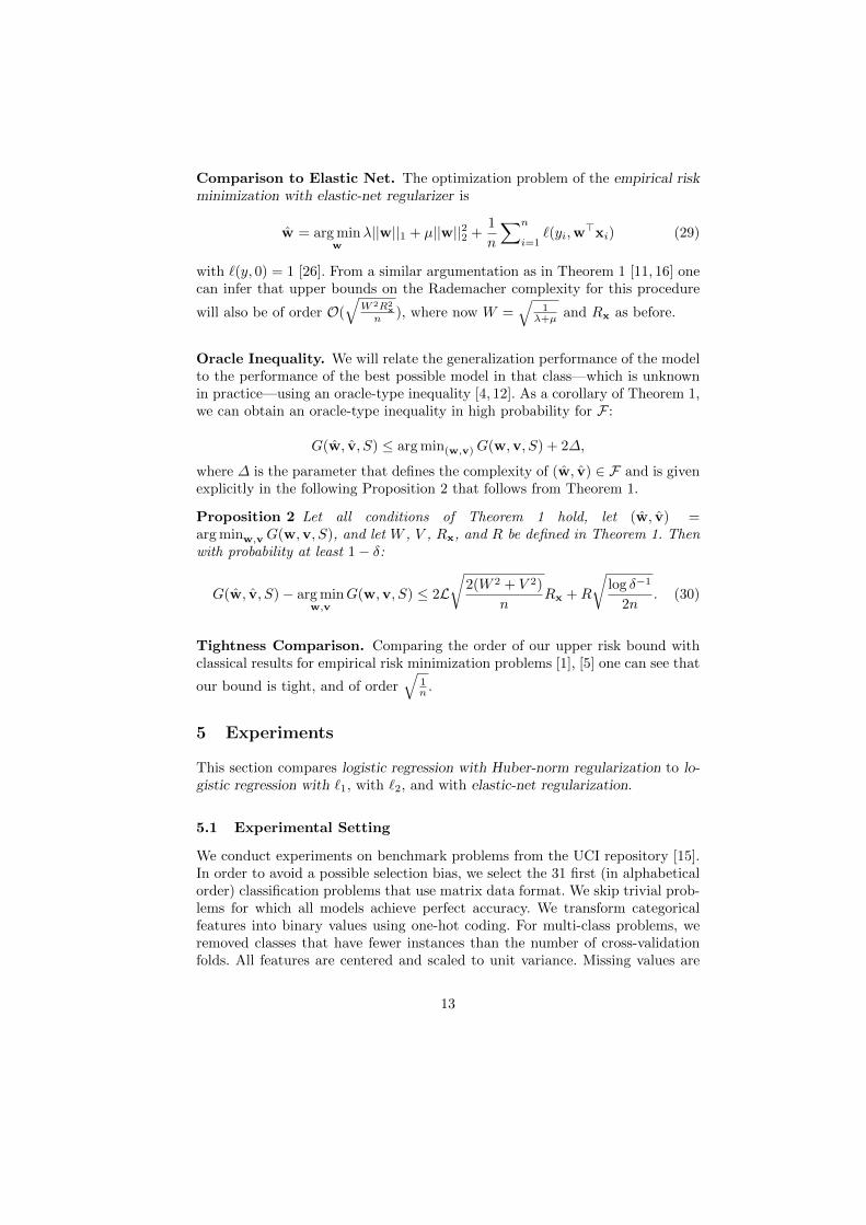
Comparison to Elastic Net. The optimization problem of the empirical riskminimization with elastic-net regularizer is

w = arg minw

λ||w||1 + µ||w||22 +1

n

∑n

i=1`(yi,w

>xi) (29)

with `(y, 0) = 1 [26]. From a similar argumentation as in Theorem 1 [11, 16] onecan infer that upper bounds on the Rademacher complexity for this procedure

will also be of order O(√

W 2R2x

n ), where now W =√

1λ+µ and Rx as before.

Oracle Inequality. We will relate the generalization performance of the modelto the performance of the best possible model in that class—which is unknownin practice—using an oracle-type inequality [4, 12]. As a corollary of Theorem 1,we can obtain an oracle-type inequality in high probability for F :

G(w, v, S) ≤ arg min(w,v)G(w,v, S) + 2∆,

where ∆ is the parameter that defines the complexity of (w, v) ∈ F and is givenexplicitly in the following Proposition 2 that follows from Theorem 1.

Proposition 2 Let all conditions of Theorem 1 hold, let (w, v) =arg minw,vG(w,v, S), and let W , V , Rx, and R be defined in Theorem 1. Thenwith probability at least 1− δ:

G(w, v, S)− arg minw,v

G(w,v, S) ≤ 2L√

2(W 2 + V 2)

nRx +R

√log δ−1

2n. (30)

Tightness Comparison. Comparing the order of our upper risk bound withclassical results for empirical risk minimization problems [1], [5] one can see that

our bound is tight, and of order√

1n .

5 Experiments

This section compares logistic regression with Huber-norm regularization to lo-gistic regression with `1, with `2, and with elastic-net regularization.

5.1 Experimental Setting

We conduct experiments on benchmark problems from the UCI repository [15].In order to avoid a possible selection bias, we select the 31 first (in alphabeticalorder) classification problems that use matrix data format. We skip trivial prob-lems for which all models achieve perfect accuracy. We transform categoricalfeatures into binary values using one-hot coding. For multi-class problems, weremoved classes that have fewer instances than the number of cross-validationfolds. All features are centered and scaled to unit variance. Missing values are

13

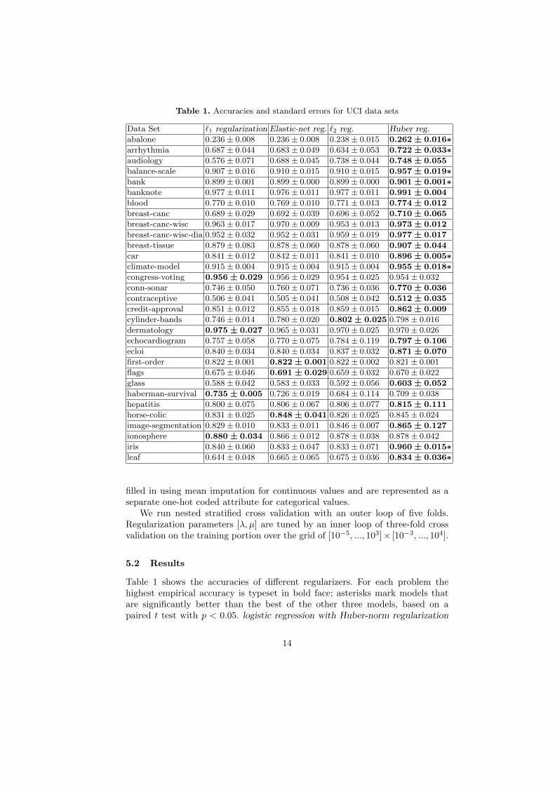
Table 1. Accuracies and standard errors for UCI data sets

Data Set `1 regularization Elastic-net reg. `2 reg. Huber reg.

abalone 0.236± 0.008 0.236± 0.008 0.238± 0.015 0.262 ± 0.016∗arrhythmia 0.687± 0.044 0.683± 0.049 0.634± 0.053 0.722 ± 0.033∗audiology 0.576± 0.071 0.688± 0.045 0.738± 0.044 0.748 ± 0.055

balance-scale 0.907± 0.016 0.910± 0.015 0.910± 0.015 0.957 ± 0.019∗bank 0.899± 0.001 0.899± 0.000 0.899± 0.000 0.901 ± 0.001∗banknote 0.977± 0.011 0.976± 0.011 0.977± 0.011 0.991 ± 0.004

blood 0.770± 0.010 0.769± 0.010 0.771± 0.013 0.774 ± 0.012

breast-canc 0.689± 0.029 0.692± 0.039 0.696± 0.052 0.710 ± 0.065

breast-canc-wisc 0.963± 0.017 0.970± 0.009 0.953± 0.013 0.973 ± 0.012

breast-canc-wisc-dia 0.952± 0.032 0.952± 0.031 0.959± 0.019 0.977 ± 0.017

breast-tissue 0.879± 0.083 0.878± 0.060 0.878± 0.060 0.907 ± 0.044

car 0.841± 0.012 0.842± 0.011 0.841± 0.010 0.896 ± 0.005∗climate-model 0.915± 0.004 0.915± 0.004 0.915± 0.004 0.955 ± 0.018∗congress-voting 0.956 ± 0.029 0.956± 0.029 0.954± 0.025 0.954± 0.032

conn-sonar 0.746± 0.050 0.760± 0.071 0.736± 0.036 0.770 ± 0.036

contraceptive 0.506± 0.041 0.505± 0.041 0.508± 0.042 0.512 ± 0.035

credit-approval 0.851± 0.012 0.855± 0.018 0.859± 0.015 0.862 ± 0.009

cylinder-bands 0.746± 0.014 0.780± 0.020 0.802 ± 0.025 0.798± 0.016

dermatology 0.975 ± 0.027 0.965± 0.031 0.970± 0.025 0.970± 0.026

echocardiogram 0.757± 0.058 0.770± 0.075 0.784± 0.119 0.797 ± 0.106

ecloi 0.840± 0.034 0.840± 0.034 0.837± 0.032 0.871 ± 0.070

first-order 0.822± 0.001 0.822 ± 0.001 0.822± 0.002 0.821± 0.001

flags 0.675± 0.046 0.691 ± 0.029 0.659± 0.032 0.670± 0.022

glass 0.588± 0.042 0.583± 0.033 0.592± 0.056 0.603 ± 0.052

haberman-survival 0.735 ± 0.005 0.726± 0.019 0.684± 0.114 0.709± 0.038

hepatitis 0.800± 0.075 0.806± 0.067 0.806± 0.077 0.815 ± 0.111

horse-colic 0.831± 0.025 0.848 ± 0.041 0.826± 0.025 0.845± 0.024

image-segmentation 0.829± 0.010 0.833± 0.011 0.846± 0.007 0.865 ± 0.127

ionosphere 0.880 ± 0.034 0.866± 0.012 0.878± 0.038 0.878± 0.042

iris 0.840± 0.060 0.833± 0.047 0.833± 0.071 0.960 ± 0.015∗leaf 0.644± 0.048 0.665± 0.065 0.675± 0.036 0.834 ± 0.036∗

filled in using mean imputation for continuous values and are represented as aseparate one-hot coded attribute for categorical values.

We run nested stratified cross validation with an outer loop of five folds.Regularization parameters [λ, µ] are tuned by an inner loop of three-fold crossvalidation on the training portion over the grid of [10−5, ..., 103]× [10−3, ..., 104].

5.2 Results

Table 1 shows the accuracies of different regularizers. For each problem thehighest empirical accuracy is typeset in bold face; asterisks mark models thatare significantly better than the best of the other three models, based on apaired t test with p < 0.05. logistic regression with Huber-norm regularization

14

achieves the highest empirical accuracy for 23 out of 31 problems; its accuracyis significantly higher than the accuracy of any other model for 8 problems. Noreference methods outperform Huber-norm regularization significantly.

The UCI repository reflects a certain distribution P (S) over data sets. Westate the null hypothesis A that the probability of Huber-norm regularizationoutperforming all three reference methods on a randomly drawn problem underP (S) does not exceed 0.5, and the null hypothesis B that the probability ofHuber-norm regularization outperforming all three reference methods on a ran-domly drawn problem under P (S) is below 0.5. We count each cross-validationfold of each UCI data set as a single observation of a binary random variable anddetermine the binomial likelihood of observing the outcomes which are reflectedin Table 1. Logistic regression with Huber-norm regularization achieves a higherempirical accuracy than all three baselines in 86 out of 155 cross-validation folds,and an equally high accuracy as the best baseline in an additional 24 cases. Wecan therefore reject the null hypothesis A at p = 0.09 and null hypothesis Beven at p < 0.001. We conclude that for the distribution of UCI problems, theHuber-norm regularization is the best-performing regularizer among the `1, `2,elastic-net and Huber regularization.

6 Conclusions

We proposed a new way of regularizing linear prediction models based on a com-bination of dense and sparse weight vectors. In more detail, we employ a linearweight vector that is the sum of two terms, w+v, where w is `2 regularized andv is `1 regularized. This results in an effective Huber-norm regularizer for w+v,which is very different from an elastic net. Starting with theoretical considera-tions, we first derived bounds on the statistical risk based on the framework ofRademacher complexities. In our subsequent experimental study, our algorithmshowed higher predictive accuracies on a majority of UCI data sets, where wecompared against `1, `2, and elastic-net regularization. In future work, we wouldlike to study extensions to non-linear kernel functions and multiple kernels [9].

Acknowledgments

MK acknowledges support from the German Research Foundation (DFG) awardKL 2698/2-1 and from the Federal Ministry of Science and Education (BMBF)award 031L0023A. The authors would like to thank Christoph Lippert, GillesBlanchard, Florian Wenzel, and Shinichi Nakajima for helpful discussions.

References

1. Bartlett, P.L., Bousquet, O., Mendelson, S.: Local rademacher complexities. Annalsof Statistics pp. 1497–1537 (2005)

2. Bartlett, P.L., Mendelson, S.: Rademacher and Gaussian complexities: Risk boundsand structural results. In: Proceedings of the International Conference on Compu-tational Learning Theory. pp. 224–240. Springer (2001)

15

3. Boyd, S., Vandenberghe, L.: Convex Optimization. Cambridge University Press(2004)

4. Clarke, B., Fokoue, E., Zhang, H.: Principles and Theory for Data Mining andMachine Learning. Springer Verlag (2009)

5. Devroye, Luc and Lugosi, Gabor: Lower bounds in pattern recognition and learn-ing. Pattern Recognition 28(7) (1995)

6. Hailong, H., Haien, L., Jianwei, L.: P-norm regularized SVM classifier by non-convex conjugate gradient algorithm. In: Proceedings of the Chinese Control andDecision Conference. vol. 3, pp. 2685–2690. IEEE (2013)

7. Huber, P.: Robust estimation of a location parameter. Annals of MathematicalStatistics 53, 73–101 (1964)

8. Huber, P.J.: Robust statistics. Springer (2011)9. Kloft, M., Brefeld, U., Sonnenburg, S., Zien, A.: lp-Norm Multiple Kernel Learning.

Journal of Machine Learning Research 12, 953–997 (2011)10. Kloft, M., Brefeld, U., Laskov, P., Muller, K.R., Zien, A., Sonnenburg, S.: Efficient

and accurate lp-norm multiple kernel learning. In: Advances in Neural InformationProcessing Systems 22, pp. 997–1005. Curran Associates, Inc. (2009)

11. Kloft, M., Ruckert, U., Bartlett, P.L.: A unifying view of multiple kernel learn-ing. In: Proceedings of the European Conference on Machine Learning, pp. 66–81.Springer (2010)

12. Koltchinskii, V.: Oracle Inequalities in Empirical Risk Minimization and SparseRecovery Problems, vol. 2033. Springer (2011)

13. Koshiba, Y., Abe, S.: Comparison of l1 and l2 support vector machines. In: Pro-ceedings of the International Joint Conference on Neural Networks. vol. 3, pp.2054–2059. IEEE (2003)

14. Kujala, J., Aho, T., Elomaa, T.: A walk from 2-norm SVM to 1-norm SVM. In:Proceedings of the IEEE Conference on Data Mining. pp. 836–841. IEEE (2009)

15. Lichman, M.: UCI machine learning repository (2013),http://archive.ics.uci.edu/ml

16. Mohri, M., Rostamizadeh, A., Talwalkar, A.: Foundations of Machine Learning.MIT press (2012)

17. Owen, A.: A robust hybrid of lasso and ridge regression. Contemporary Mathe-matics 443, 59–72 (2007)

18. Robert, T.: The Lasso method for variable selection in the Cox model. Statisticsin Medicine 16, 385–395 (1997)

19. Steinwart, I., Christmann, A.: Support Vector Machines. Springer Science & Busi-ness Media (2008)

20. Suykens, J.A., De Brabanter, J., Lukas, L., Vandewalle, J.: Weighted least squaressupport vector machines: robustness and sparse approximation. Neurocomputing48(1), 85–105 (2002)

21. Unger, M., Pock, T., Werlberger, M., Bischof, H.: A convex approach for variationalsuper-resolution. In: Joint Pattern Recognition Symposium. pp. 313–322 (2010)

22. Vapnik, V.: The nature of statistical learning theory. Springer (1995)23. Wang, L., Jia, H., Li, J.: Training robust support vector machine with smooth

ramp loss in the primal space. Neurocomputing 71(13), 3020–3025 (2008)24. Yuille, A.L., Rangarajan, A.: The concave-convex procedure. Neural computation

15(4), 915–936 (2003)25. Zhu Ji, S.R., Trevor, H., Rob, T.: 1-norm support vector machines. Advances of

Neural Information Processing Systems (2004)26. Zou, H., Hastie, T.: Regularization and variable selection via the elastic net. Jour-

nal of the Royal Statistical Society: Series B 67(2), 301–320 (2005)

16