Human Action Recognition using Bag of Features

Jesper Birksø BækdahlMaster’s Thesis

May 2012

Supervisor: Thomas Moeslund

Vision, Graphics and Interactive SystemsAalborg University

Elektroniske SystemerInstitut 8Fredrik Bajers Vej 79220 Aalborg Øhttp://es.aau.dk/

Title:Human Action Recognitionusing Bag of Features

Project period:9 - 10. semester,August 2011 - May 2012

Project group:11gr924

Group members:Jesper Birksø Bækdahl

Supervisor:Thomas Moeslund

Pages: 51

Finished: May 31st 2012

Abstract:

This thesis explores the popular bag-of-features framework for human action recogni-tion. Different feature detectors and descrip-tors are described and compared.The combination of the Harris3D detector andthe HOG/HOF descriptor is chosen for use inthe experimental setup. Unsupervised and su-pervised classification methods are comparedto show the difference in performance. Thesupervised algorithm used is a support vectormachine, and the unsupervised algorithms arek-means clustering, and affinity propagation,where the latter has not been used before foraction recognition. The algorithms are testedon two different datasets. The simple KTHdataset with 6 classes, and the more compli-cated UCF50 with 50 classes.The SVM classification obtains good resultson both KTH and UCF50. Of the two unsu-pervised methods, affinity propagation obtainsthe best performance. SVM outperforms bothof the unsupervised algorithms. The strategyused for building the vocabulary, which is acentral part of the bag-of-features frameworkis tested. The results show, that increasingthe number of words will slightly increase theclassifier performance.

1

Preface

This report documents the Master’s thesis: “Human Action Recognition using Bag of Features”during the 9th and 10th semester of the specialisation: “Vision Graphichs and Interactive Sys-tems”.The software developed in this project has been submitted to the Aalborg University projectdatabase1, and can also be found on the authors website2.The front page of shows examples of different actions from a dataset of still images presented in[7].

Acknowledgements

I would like to thank:Dr. Mubarak Shah and University of Central Florida for hosting me from autumn 2011 to summer2012. The inspiration and help i received there has been a great support during this project.My supervisor Thomas Moeslund for making it possible for me to go to UCF, and for supportingme both professionally and personally during my stay.Bhaskar Chakraborty and Michael Holte for supplying me with action recognition code and ad-vice.

1http://projekter.aau.dk/projekter/2http://kom.aau.dk/˜baekdahl/masters/

3

Contents

Contents 5

1 Introduction 7

2 Analysis 9

3 Feature Detectors 19

4 Feature Descriptors 23

5 Feature comparison 27

6 Representation 29

7 Supervised Learning 31

8 Unsupervised Learning 35

9 Results 39

10 Conclusion 47

Bibliography 49

5

Chapter 1

Introduction

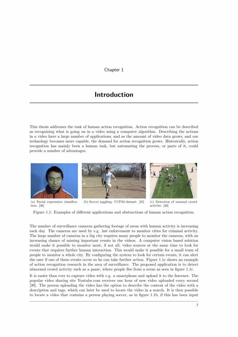
This thesis addresses the task of human action recognition. Action recognition can be describedas recognizing what is going on in a video using a computer algorithm. Describing the actionsin a video have a large number of applications, and as the amount of video data grows, and ourtechnology becomes more capable, the demand for action recognition grows. Historically, actionrecognition has mainly been a human task, but automating the process, or parts of it, couldprovide a number of advantages.

(a) Facial expression classifica-tion. [36]

(b) Soccer juggling. UCF50 dataset. [25] (c) Detection of unusual crowdactivity. [26]

Figure 1.1: Examples of different applications and abstractions of human action recognition.

The number of surveillance cameras gathering footage of areas with human activity is increasingeach day. The cameras are used by e.g. law enforcement to monitor cities for criminal activity.The large number of cameras in a big city requires many people to monitor the cameras, with anincreasing chance of missing important events in the videos. A computer vision based solutionwould make it possible to monitor most, if not all, video sources at the same time to look forevents that requires further human interaction. This would make it possible for a small team ofpeople to monitor a whole city. By configuring the system to look for certain events, it can alertthe user if one of these events occur so he can take further action. Figure 1.1c shows an exampleof action recognition research in the area of surveillance. The proposed application is to detectabnormal crowd activity such as a panic, where people flee from a scene as seen in figure 1.1c.It is easier than ever to capture video with e.g. a smartphone and upload it to the Internet. Thepopular video sharing site Youtube.com receives one hour of new video uploaded every second[39]. The person uploading the video has the option to describe the content of the video with adescription and tags, which can later be used to locate the video in a search. It is then possibleto locate a video that contains a person playing soccer, as in figure 1.1b, if this has been input

7

CHAPTER 1. INTRODUCTION

Figure 1.2: Children playing a game controlled via motion capture by Microsoft Kinect [21].

in the title and/or description of the video. But what if a user is interested in searching for allgoals or free kicks in a soccer match between two teams? It is not common for a descriptionof a video to include this many details because the user who uploaded the video has to inputit manually. This kind of detailed search could be possible if the video had been annotated byan action recognition system that recognizes such events. It could even be possible to locate theexact time instant where a goal happens. Using action recognition for video categorization andannotation will enable us to make better use of the vast amounts of video data in ways that arenot possible today.The progress in video capture and processing hardware has also spawned products like the Mi-crosoft Kinect, that acts as a motion capture controller for a gaming console. The Kinect combinesaction, gesture and voice recognition for a total interactive experience, as seen in figure 1.2, with-out the use of an old-fashioned joystick. The system is robust enough to work in a normal livingroom with varying lighting and background clutter. The idea of gesture control is extending todevices such as televisions, where we soon will be able to change channels or lower the volumewith the use of gestures.Action recognition remains a challenging problem, and so far only the tip of the iceberg has beenrevealed. Most of the existing solutions only work for simple or synthetic scenes which have beencreated for the purpose of testing action recognition algorithms. The best solutions still requirelarge amounts of supervised training data, which is expensive to obtain. This leads us to thefollowing initiating problem:

• What is the state of the art in human action recognition, and what is the bestway to take advantage of the large number of unlabelled videos?

8

Chapter 2

Analysis

This section describes the different methods and algorithms used for Human Action Recognition.Different datasets are presented to show that action recognition has evolved from classifying simplesynthetic datasets to new challenging realistic datasets. The main frameworks and models used torepresent an action recognition problem are presented in section 2.3 along with the bag-of-featuresframework which is the one used in this thesis. Finally a problem statement is presented to givea concise description of the contribution and scope of this thesis.

2.1 Human Action Recognition

Initialisation Tracking Pose Estimation Recognition

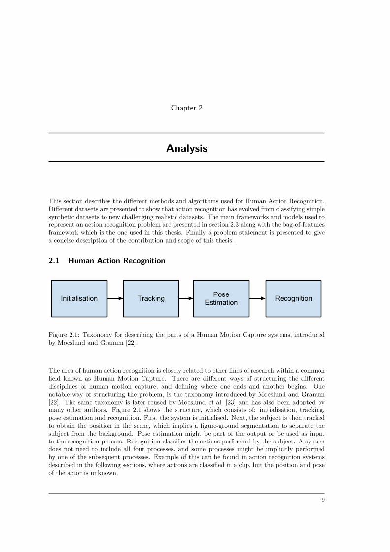
Figure 2.1: Taxonomy for describing the parts of a Human Motion Capture systems, introducedby Moeslund and Granum [22].

The area of human action recognition is closely related to other lines of research within a commonfield known as Human Motion Capture. There are different ways of structuring the differentdisciplines of human motion capture, and defining where one ends and another begins. Onenotable way of structuring the problem, is the taxonomy introduced by Moeslund and Granum[22]. The same taxonomy is later reused by Moeslund et al. [23] and has also been adopted bymany other authors. Figure 2.1 shows the structure, which consists of: initialisation, tracking,pose estimation and recognition. First the system is initialised. Next, the subject is then trackedto obtain the position in the scene, which implies a figure-ground segmentation to separate thesubject from the background. Pose estimation might be part of the output or be used as inputto the recognition process. Recognition classifies the actions performed by the subject. A systemdoes not need to include all four processes, and some processes might be implicitly performedby one of the subsequent processes. Example of this can be found in action recognition systemsdescribed in the following sections, where actions are classified in a clip, but the position and poseof the actor is unknown.

9

CHAPTER 2. ANALYSIS

2.2 Datasets

In this section four action recognition datasets are presented: Weizmann, KTH, Hollywood andUCF50. Weizmann and KTH are both scripted datasets, where the actors have been told toperform a specific action in a controlled setting with only minor changes in viewpoint, backgroundand illumination. This makes them easy to classify, and every state of the art algorithm is able toget over 90% average precision, which makes these datasets less interesting to use as a benchmark.Developing an algorithm that solves these datasets does not necessarily mean that the algorithmwill be good at solving the more advanced datasets because the challenges there are different.Hollywood and UCF50 have been sampled from existing video, that was not created for thepurpose of action recognition. This provides a more realistic environment but also much morechallenging. The huge differences in the videos mean that an algorithm have very few conditionsto rely on. It has to be adaptable to different viewpoints, cluttered backgrounds, multiple actors,occlusions, etc. These conditions makes it much harder to obtain good results, especially foralgorithms that depend on e. g. being able to get a good segmentation.

2.2.1 WeizmannThe Weizmann dataset, figure 2.2 [1], contains 10 different actions: walk, run, jump, gallopsideways, bend, one-hand wave, two-hands wave, jump in place, jumping jack and skip. Eachaction is performed by 10 different actors resulting in a total of 100 clips. The viewpoint andbackground are static and equal for all clips.

11

3 11

5

inria

-004

5965

3, v

ersi

on 1

- 24

Feb

201

0

Figure 2.2: Example frames from Weizmann dataset.

2.2.2 KTHKTH, figure 2.3 [32], contains 6 different actions: walking, jogging, running, boxing, hand wavingand hand clapping. The actions are performed by 25 different actors in four different scenarios:outdoors, outdoors with zooming, outdoors with different clothing and indoors. Compared toWeizmann, KTH has considerable amounts of intraclass differences. There are differences induration and somewhat in viewpoint.

2.2.3 HollywoodThe original Hollywood dataset, figure 2.4 [16], contains 8 different actions. It has later beenextended with 4 additional actions [20]. The actions are: answer phone, get out of car, handshake,hug, kiss, sit down, sit up, stand up, drive car, eat, fight, run. There are approximately 150samples per class. All actions are taken from 69 different Hollywood movies, resulting in hugevariety between viewpoint, background and action performance.

10

2.3. ACTION RECOGNITION METHODS

inria

-004

5965

3, v

ersi

on 1

- 24

Feb

201

0

Figure 2.3: Example frames from KTH dataset.

Figure 2.4: Example frames from Hollywood dataset.

2.2.4 UCF50UCF50 [25] is an extension of the UCF Youtube dataset. The dataset has 50 different actionshaving at least 100 clips for each action for a total of 6681 clips. The actions are all user-submittedvideos from Youtube.com, and by that nature very different from each other. Many of the videosinclude large amounts of camera motion, illumination changes and cluttered backgrounds.The actions in UCF50 are: baseball pitch, basketball shooting, bench press, biking, biking, bil-liards shot,breaststroke, clean and jerk, diving, drumming, fencing, golf swing, playing guitar,high jump, horse race, horse riding, hula hoop, javelin throw, juggling balls, jump rope, jumpingjack, kayaking, Lunges, military parade, mixing batter, nun chucks, playing piano, pizza tossing,pole vault, pommel horse, pull ups, punch, push ups, rock climbing indoor, rope climbing, row-ing, salsa spins, skate boarding, skiing, skijet, soccer juggling, swing, playing tabla, taichi, tennisswing, trampoline jumping, playing violin, volleyball spiking, walking with a dog, and yo yo.

2.3 Action Recognition Methods

This section provides an overview of the different approaches to action recognition, taken fromvarious surveys [22, 23, 27, 37, 41].

2.3.1 Body modelsOne of the most intuitive approaches to action recognition is body models. To recognize an actionperformed by a human, the different body parts are detected according to a body model. Themodel constraints how one body part is positioned compared to the others, e. g. a foot can not

11

CHAPTER 2. ANALYSIS

Figure 2.5: Example frames from UCF50 dataset.

be connected to an arm, and the angle between the upper arm and forearm can only be withinthe range that is physically possible with the human join configuration. The recognition worksby comparing the movement performed by the body model extracted from a video with existingground truth body models. The ground truth body models can be generated synthetically or takenfrom motion capture of a human performing the action in a controlled setting, where markers orother remedies are used to obtain a ground truth body model. There are two common approachesin the use of body models: recognition by reconstruction and direct recognition.

inria

-004

5965

3, v

ersi

on 1

- 24

Feb

201

0

(a) Moving Light Display(MLD).[12]

inria

-004

5965

3, v

ersi

on 1

- 24

Feb

201

0

(b) Body model based on rectan-gular patches. [28]

Figure 2.6: Examples of body models.

Recognition by reconstruction is a 3D approach, where the motion of the body is captured and a3D model of the body is estimated. This is a challenging approach because of the large numberof degrees-of-freedoms of the human body. Marr and Nishihara [19] proposed a body modelconsisting of cylindrical primitives . Using such a model is called a top down approach. Thisrefers to the fact that the 3D body models are found by matching 2D projections sampled inthe search space of joint configurations. The opposite method is called bottom-up and works bytracking body parts in 2D and subsequently lifting the 2D model into 3D. An example of the

12

2.3. ACTION RECOGNITION METHODS

bottom-up approach is seen in figure 2.6b, where the body parts are tracked using rectangularpatches and lifted into 3D using an orthographic camera model.Direct recognition works on a 2D model without lifting this model into 3D. Many different 2Dmodels have been investigated. Some models consist of anatomical landmarks like joint positions.This was pioneered by Johansson [12], who showed that humans can recognize actions merelyfrom the motion of a few moving light displays(MLD) attached to the human body as seen infigure 2.6a. Other models use stick figures which can be detected from a space-time volume.

2.3.2 Holistic approaches

The holistic approach, also referred to as global model or image model, encodes the whole subjectas one entity. This often involves locating a ROI via segmentation and/or tracking. Commonrepresentations are silhouettes, edges or optical flow. This representation can be much simplerand faster to compute than body model, but still be as discriminative in problems consisting of alarge number of classes.

!"#$%&'(&)*+ (," '%"$&#" ',-#" ,-# .&((." "//"$( )* (," #,-'"!"#$%&'(&)*0

1," -"%)2&$# &3-4"%5 '%)6&!"# "7-3'."# )/ 8,5 ,-6&*42)(, (," 9:; -*! 9<; &# 6-.=-2." "6"* (,)=4, (," 9:; $-*2" $)*#(%=$("! 25 (,%"#,).!&*4 (," 9<;0 >&40 ? #,)8# (,"9:; -*! 9<; /)% 3)6"# @+ A+ -*! BC0 D)(" (,-( 3)6" A -*!BC ,-6" E=&(" #&3&.-% 9:;# 5"( !&#(&*$( 9<;#F 3)6"# @ -*! A,-6" #&3&.-% 9<;# &* ("%3# )/ 8,"%" (," 3-G)%&(5 )/ &3-4""*"%45 &# .)$-("! 5"( !&#'.-5 E=&(" !&#(&*$( 9:;#0 H"$-=#"(," 9:; -*! 9<; '%)G"$(&)* /=*$(&)*# $-'(=%" (8) !&#(&*$($,-%-$("%&#(&$# )/ (," 3)(&)*IJ8,"%"K -*! J,)8+K %"#'"$L(&6".5I(," #,-'" !"#$%&'()%# )/ (,"#" (8) &3-4"# !&#$%&3&L*-(" !&//"%"*(.50

>)% (,&# "7'"%&3"*(+ (," ("3')%-. #"43"*(-(&)* -*!#"."$(&)* )/ (," (&3" 8&*!)8 )6"% 8,&$, () &*("4%-(" 8"%"'"%/)%3"! 3-*=-..50 M-("%+ 8" 8&.. !"(-&. - #"./L#"43"*(&*4+(&3"L#$-.&*4 %"$)4*&(&)* #5#("3 NO"$(&)* PQ0 1," )*.5 '%"L'%)$"##&*4 !)*" )* (," !-(- 8-# () %"!=$" (," &3-4"%"#).=(&)* () R@S 7 @AS /%)3 (," $-'(=%"! ?AS 7 ATS0 1,&# #("',-! (," "//"$( )/ *)( )*.5 %"!=$&*4 (," !-(- #"( #&U" 2=( -.#) )/'%)6&!&*4 #)3" .&3&("! 2.=%%&*4 8,&$, "*,-*$"# (," #(-2&.&(5)/ (," 4.)2-. #(-(&#(&$#0

V" $)*#(%=$("! (," ("3')%-. ("3'.-(" /)% "-$, 6&"8 )/"-$, 3)6" -*! (,"* $)3'=("! (," <= 3)3"*(# )* "-$,$)3')*"*(0 1) !) - =#"/=. 9-,-.-*)2&# '%)$"!=%" 8)=.!%"E=&%" 8-($,&*4 #"6"%-. !&//"%"*( '")'." '"%/)%3&*4 (,"#-3" 3)6"3"*(#+ (,&# 3=.(&#=2G"$( -''%)-$, &# (-W"* &* (,"*"7( #"$(&)* 8,"%" 8" !"6".)' - %"$)4*&(&)* '%)$"!=%"=#&*4 - /=.. $)6-%&-*$" NO"$(&)* PQ0 ;*#("-!+ ,"%" 8" !"#&4*(," "7'"%&3"*( () 2" - 3"-#=%"3"*( )/ $)*/=#&)*0 X *"8("#( #=2G"$( '"%/)%3"! "-$, 3)6" -*! (," &*'=( !-(- 8-#%"$)%!"! 25 (8) $-3"%-# 6&"8&*4 (," 3)6"3"*( -(-''%)7&3-(".5 !"! () ."/( -*! #"! () (," %&4,( )/ (," #=2G"$(01," ("3')%-. ("3'.-(" /)% "-$, )/ (," (8) 6&"8# )/ (," ("#(

&*'=( 3)6"3"*(# 8-# $)*#(%=$("! -*! (," -##)$&-("!3)3"*(# $)3'=("!0

Y=% /&%#( ("#( =#"# )*.5 (," ."/( N!"!Q $-3"%- -# &*'=( -*!3-($,"# -4-&*#( -.. #"6"* 6&"8# )/ -.. BT 3)6"# NB@? ()(-.Q0;* (,&# "7'"%&3"*(+ 8" =#"! )*.5 )*" &*#(-*$" )/ "-$, 6&"8Z3)6" '-&%0 V" #"."$( -# - 3"(%&$ - !""#$% &*!"'"*!"*(9-,-.-*)2&# !&#(-*$"I=#&*4 (," #-3" !&-4)*-. $)6-%&-*$"3-(%&7 /)% -.. (," $.-##"# -# 4"*"%-("! 25 ')).&*4 -.. (,"!-(-I() -$$)33)!-(" 6-%&-(&)*# &* 3-4*&(=!" )/ (,"3)3"*(#0 1-2." B !&#'.-5# (," %"#=.(#0 ;*!&$-("! -%" (,"!&#(-*$" () (," 3)6" $.)#"#( () (," &*'=( N-# 8".. -# &(#&*!"7Q+ (," !&#(-*$" () (," $)%%"$( 3-($,&*4 3)6"+ (,"3"!&-* !&#(-*$" N() 4&6" - #"*#" )/ #$-."Q+ -*! (," %-*W&*4)/ (," $)%%"$( 3)6" &* ("%3# )/ ."-#( !&#(-*$"0

1," /&%#( %"#=.( () *)(" &# (,-( B@ )/ BT 3)6"# -%" $)%%"$(.5&!"*(&/&"! =#&*4 (," #&*4." 6&"80 1,&# '"%/)%3-*$" &# E=&("4))! $)*#&!"%&*4 (," $)3'-$(*"## )/ (," %"'%"#"*(-(&)* N-()(-. )/ BA 3)3"*(# /%)3 (8) $)%%".-("! 3)(&)* &3-4"#Q -*!(," #&U" -*! #&3&.-%&(5 )/ (," (-%4"( #"(0 O"$)*!+ &* (," (5'&$-.#&(=-(&)* &* 8,&$, (," 2"#( 3-($, &# *)( (," $)%%"$( 3)6"+ (,"!&//"%"*$" &* !&#(-*$"# /%)3 (," &*'=( () (," $.)#"#( 3)6"6"%#=# (," $)%%"$( 3)6" &# #3-.. $)3'-%"! () (," 3"!&-*!&#(-*$"0 :7-3'."# )/ (,&# &*$.=!" ("#( 3)6"# B+ [+ BR+ B?+ -*!BT0 ;* /-$(+ /)% 3)6"# B+ B?+ -*! BT (," !&//"%"*$" &# *"4.&4&2."0

1) -*-.5U" (," $)*/=#&)* !&//&$=.(&"# /=%(,"%+ $)*#&!"% (,""7-3'." #,)8* &* >&40 C0 \&#'.-5"! ,"%"+ ."/( () %&4,(+ -%" (,"&*'=( 9<; NW*)8* () 2" 3)6" BR -( 6&"8 -*4." !"!Q+ (,"$.)#"#( 3-($, 9<; N3)6" ? -( 6&"8 -*4.""!Q+ -*! (," J$)%%"$(K3-($,&*4 9<; )/ 3)6" BR0 1," '%)2."3 &# (,-( -* -.("%*-(&6"6&"8 )/ - !&//"%"*( 3)6"3"*( '%)G"$(# &*() - ("3')%-.

!"!#$% &'( (&)#*+ ,-. /.$"0'#,#"' "1 -23&' 3").3.', 2*#'0 ,.34"/&5 ,.345&,.* 678

19:; 7; $<=>?@9A<B <C 3.# ?BD 3-#; 2BDE@ ?B 3.# DEAF@9>G9<B =<HEA I?BD JK ?@E E?A9LM F<BCNAEDO NBDE@ GPE 3-#Q =<HEA 6 ?BD I ?@E A9=9L?@;!EF?NAE GPE :L<R?L AP?>E DEAF@9>G9<BA ?@E SE9:PGED RM GPE >9TEL H?LNEAQP?H9B: R<GP 9=?:EA M9ELDA =<@E D9AF@9=9B?G9<B ><SE@;

,&!5. J,EAG /EANLGA 2A9B: "BE $?=E@? ?G !"! "CC 1@<BG?L

!"#$ %&' #&%%()*&+,) -& &+( -()- .&/( "+, 01/() -$( ,1)-"+#( -& -$(+("%()- .&/( 2"+, 1-) 1+,(345 -$( ,1)-"+#( -& -$( #&%%(#- ."-#$1+0 .&/(5-$( .(,1"+ ,1)-"+#(5 "+, -$( %"+61+0 &7 -$( #&%%(#- .&/(8

(a) MEI and MHI for 3 different ballet actions.[2]

(b) Space-time shapes. [1]

Figure 2.7: Examples of holistic methods.

Silhouettes have proved to be a useful global representation of a subject. The silhouette canbe found by background subtraction, and can be encoded in a contour or by the area inside.Silhouettes are insensitive to color, texture and contrast changes, but have problems with self-occlusion and depend on robust segmentation. An early examples of the use of silhouettes, extractssilhouettes from each frame of the video which results in a motion energy image(MEI). A motionhistogram image(MHI) is also computed which is function of the history at that pixel over timeas seen in figure 2.7a. Silhouettes can also be combined over time to form space-time shapes asshown in figure 2.7b.Other holistic approaches are based on flow and gradients. This works by extracting optical flowor gradients within the ROI or in the entire image. A grid is often used to divide the extractionarea to partly overcome partial occlusions and changes in viewpoint. This grid can be definedin different ways. Danafar and Gheissari [6] divides the ROI into horizontal slices correspondingapproximately to head, body and leg, and use optical flow extracted in these areas. Histogramsof oriented gradients(HOG) have also been used to represent the ROI by a number of histogramsthat consists of gradient directions.

13

CHAPTER 2. ANALYSIS

2.3.3 Local featuresLocal features describes the action in a video as a set of local descriptors instead of one globaldescriptor as in the global approach. These local descriptors are combined in one representationof the video, which can be done in different ways to either ignore, or maintain the spatial and/ortemporal relationship between the features. The features can either be extracted densely or atspatio-temporal interest points(STIPs), which are points that contain information important todetermining the action in the video.STIP detectors usually works by evaluating the response of one or more filters applied to the video.Laptev [14] extended the Harris corner detector to 3D and detects STIPs by finding local maximaof the extended corner function. Dollar et al. [8] uses a Gabor filter in the temporal dimension,and overcomes the problem of too few interest points that predecessors had. Rapantzikos et al.[29] apply discrete wavelet transform in spatial and temporal direction of the video, and uses afiltered version to detect salient regions. Willems et al. [38] identifies saliency as the determinantof a 3D Hessian matrix. Chakraborty et al. [3] filters out points that belong to the backgroundusing a surround suppression measure. The final points are selected based on point matching andGabor filtering in the temporal direction.

of the cuboid over multiple scales and locations in both space andtime. In related work by Scovanner et al. [126], the SIFT descriptor[79] is extended to 3D. Wang et al. [151] compared local descrip-tors and found that, in general, a combination of image gradientand flow information resulted in the best performance.

Several approaches combine interest point detection and thecalculation of local descriptors in a feed-forward framework. Forexample, Jhuang et al. [58] use several stages to ensure invarianceto a number of factors. Their approach is motivated by the humanvisual system. At the lowest level, Gabor filters are applied to denseflow vectors, followed by a local max operation. Then the re-sponses are converted to a higher level using stored prototypesand a global max operation is applied. A second matching stagewith prototypes results in the final representation. The work in[96] is similar in concept, but uses different window settings.Schindler and Van Gool [124] extend the work by Jhuang et al.[58] by combining both shape and flow responses. Escobar et al.[31] use motion-sensitive responses and also consider interactionsbetween cells, which allows them to model more complex proper-ties such as motion contrasts.

Comparing sets of local descriptors is not straightforward due tothe possibly different number and the usually high dimensionalityof the descriptors. Therefore, often a codebook is generated byclustering patches and selecting either cluster centers or the clos-est patches as codewords. A local descriptor is described as a code-word contribution. A frame or sequence can be represented as abag-of-words, a histogram of codeword frequencies (e.g. [95,125]).

2.2.3. Local grid-based representationsSimilar to holistic approaches, described in Section 2.1.1, grids

can be used to bin the patches spatially or temporally. Comparedto the bag-of-words approach, using a grid ensures that spatialinformation is maintained to some degree.

In the spatial domain, _Ikizler and Duygulu [56] sample orientedrectangular patches, which they bin into a grid. Each cell has anassociated histogram that represents the distribution of rectangleorientations. Zhao and Elgammal [180] bin local descriptorsaround interest points in a histogram with different levels ofgranularity. Patches are weighted according to their temporal dis-tance to the current frame.

Nowozin et al. [98] use a temporal instead of a spatial grid. Thecells overlap, which allows them to overcome small variations inperformance. Observations are described as PCA-reduced vectorsaround extracted interest points, mapped onto codebook indices.

Laptev and Pérez [74] bin histograms of oriented gradients andflow, extracted at interest points, into a spatio-temporal grid. Thisgrid spans the volume that is determined based on the position andsize of a detected head. The distribution of these histograms isdetermined for every spatio-temporal cell in the grid. Three differ-ent block types are used to form the new feature set. These typescorrespond to a single cell, a concatenation of two temporallyneighboring cells and a concatenation of spatially neighboringcells. A subset of all possible blocks within the grid is selectedusing AdaBoost. A larger number of grid types, with different spa-tial and temporal divisions and overlap settings, is evaluated in[73]. Flow descriptors from [27] are used by Fathi and Mori [35],who select a discriminative set of low-level flow features withinspace–time cells which form an overlapping grid. In a subsequentstep, a set of these mid-level features is selected using the Ada-Boost algorithm. In the work by Bregonzio et al. [13], no local im-age descriptor are calculated. Rather, they look at the number ofinterest points within cells of a spatio-temporal grid with differentscales. This approach is computationally efficient but depends onthe number and relevancy of the interest points.

2.2.4. Correlations between local descriptorsGrid-based representations model spatial and temporal rela-

tions between local descriptors to some extent. However, theyare often redundant and contain uninformative features. In thissection, we describe approaches that exploit correlations betweenlocal descriptors for selection or the construction of higher-leveldescriptors.

Scovanner et al. [126] construct a word co-occurrence matrix,and iteratively merge words with similar co-occurrences untilthe difference between all pairs of words is above a specifiedthreshold. This leads to a reduced codebook size and similaractions are likely to generate more similar distributions of code-words. Similar in concept is the work by Liu et al. [76], who usea combination of the space–time features and spin images, whichglobally describe an STV. A co-occurrence matrix of the featuresand the action videos is constructed. The matrix is decomposedinto eigenvectors and subsequently projected onto a lower-dimen-sional space. This embedding can be seen as feature-level fusion.Instead of determining pairs of correlated codewords, Patron-Perezand Reid [106] approximate the full joint distribution of featuresusing first-order dependencies. Features are binary variables thatindicate the presence of a codeword. A maximum spanning treeis formed by analyzing a graph between all pairs of features. The

xtime

y

xtime

y

xtime

y

xtime

y

Fig. 3. Extraction of space–time cuboids at interest points from similar actions performed by different persons (reprinted from [71], ! Elsevier, 2007).

R. Poppe / Image and Vision Computing 28 (2010) 976–990 981

Figure 2.8: Extraction of space–time cuboids at interest points from similar actions performed bydifferent persons [15].

The feature descriptor should capture the important information in the area around a STIP andrepresent it in a sparse and discriminative way. The size of the volume or patch used to computethe descriptor is usually determined by the detection scale. Examples of volumes extracted atinterest points is seen in figure 2.8. Schuldt et al. [32] uses patches based on normalized derivativeswith respect to space and time. Similar to the global approach, descriptors can also be grid-basedlike HOG [5]. Many of these grid-based methods have also been extended to 3D. ESURF featuresis an extension of the SURF descriptor to 3D introduced in [38]. HOG is extended to HOG3D byKlaser et al. [13]. A 3D version of the popular 2D descriptor SIFT was introduced by Scovanneret al. [33].The set of feature descriptors in a video needs to be combined to form a representation thatmakes is possible to compare videos to each other. A popular representation is the bag-of-featuresrepresentation [32], where a vocabulary is generated by clustering feature descriptors from allpossible classes into a number of words. Each video is then represented by a histogram thatcounts the number of occurrences of each possible word in the video. The histograms can then beused to train a classifier, like e. g. a support vector machine(SVM).

2.3.4 Un- and semisupervised approachesThe amounts of unlabelled data is increasing and there is a high cost of labelling the large amountsof data needed for typical machine learning applications. This makes methods that require little orno supervised data become attractive. Supervised methods have so far received far more attention,but the interests in un- and semisupervised methods is growing.

14

2.4. FRAMEWORK

Niebles et al. [24] proposed unsupervised classification of bag-of-features histogram using latenttopic models such as the probabilistic Latent Semantic Analysis(pLSA) model and Latent DirichletAllocation (LDA). Savarese et al. [31] replaced bag-of-features with spatio-temporal correllogramsto better describe the temporal pattern of the features. Dueck and Frey [9] uses affinity prop-agation [10] for unsupervised learning of image categories, obtaining better results than usingk-means clustering.One of the most simple and intuitive methods for semisupervised learning is self-training. Inself-training a supervised classifier is trained on available the labelled samples. The unlabelledpoints are then classified using this weakly trained classifier, and the most confident points areused to retrain the classifier together with the labelled points. This is repeated until all points areused. Rosenberg et al. [30] used self-training for object detection. A common way of developinga semisupervised algorithm is to extend an unsupervised algorithm to respect constraints. Onenotable example is constrained expectation maximization [34].

2.4 Framework

,QSXWYLGHR )HDWXUHGHWHFWRU

6XSHUYLVHG

8QVXSHUYLVHG

)HDWXUHGHVFULSWRUV

9LGHRUHSUHVHQWDWLRQ

&ODVVLILFDWLRQ

9LGHR

9LGHR1

Figure 2.9: Human action recognition framework.

This section describes the action recognition framework that is used in this thesis. The frameworkfocuses on a subset of the methods presented in the former sections. The representation used islocal features in a bag of words framework, because it is a promising direction for describing themore advanced datasets like UCF50. Supervised and unsupervised classification will be compared,to see how training data affects the recognition rate. There has not been many attempts to dounsupervised classification within this framework, so this will be explored in this thesis by a testof the clustering algorithm: affinity propagation that, to our knowledge, has not been used beforein action recognition.The framework consists of four main components: feature detector, feature descriptor, videorepresentation and classification. The different parts of this framework can be replaced withdifferent algorithms to form different combinations and thereby produce different results.

15

CHAPTER 2. ANALYSIS

Feature detector

The first step is to detect interest points in the video, which are the positions where the featuredescriptors are computed. These points should ideally be located at places in the video where theaction is taking place.

Feature descriptor

The feature descriptor encodes the information in the area of an interest point into a representationsuited for representing the action. The feature descriptor should ideally be invariant to changeslike orientation, scale and illumination to be able to match features across different kinds of videos.

Video representation

The set of local feature descriptors in a video has to be combined into a representation that enablesthe comparison with other videos. The most popular method is the bag-of-features representation,where the spatial and temporal locations of the features are ignored. Other methods tries to takethe relationship between the features into account.

Classification

The classification step can be: unsupervised, semi-supervised or supervised.In the unsupervised approach, we assume that we do not know the labels of any of the videos.The videos are then grouped together based on their similarities. The number of groups used forunsupervised learning can be given as part of the problem, or can be dynamic where differentpartitions of videos corresponds to different semantically meanings.In semi-supervised classification there is some prior knowledge about the videos, which can consistof a few labelled samples, or e. g. a constraint saying that sample a and b are from different classeswithout giving the label. Semi-supervised learning is not explored further in this thesis.Supervised classification uses a large number of training samples to train a classifier.

2.5 Problem Statement

The analysis described different approaches to action recognition, and a specific framework waschosen to examine further. The rest of this thesis tries to answer the following problem statement:

• What are the pros and cons of the different components in the bag-of-featuresframework, and which combination yields the best performance?

– How does unsupervised clustering algorithms compare to supervised classification?– How does the performance of the methods change when the complexity of the dataset

change?– What is the best strategy for bag-of-features vocabulary building?

2.5.1 Scope of this thesis

This thesis compares methods within the beforementioned framework, and does then not considerall other possible action recognition frameworks beyond the brief introduction given in section 2.3.All video clips are presumed to contain exactly one action being performed, i. e. the describedframework does not worry about action detection, multiple actors or multiple actions in the sameclip.

16

2.6. THESIS OUTLINE

2.6 Thesis outline

The rest of this thesis seeks to answer the questions asked in the above problem statement.Notable examples of each component of the bag-of-features framework is described. Section 3and 4 presents feature detectors and descriptors, respectively. A comparison of detector anddescriptor combinations is given in section 5. The bag of words representation is described insection 6. Supervised and unsupervised classification is presented in section 7 and 8, respectively.Finally the results of classification using various combinations of methods are presented in 9.

17

Chapter 3

Feature Detectors

This section describes in detail some of the more notable local feature detectors. A feature detectorfinds the points in the video where features are going to be extracted. These points are known asSpatio-Temporal Interest Points(STIPs). A STIP is a point in space and time (x, y, t) that hashigh saliency. High saliency means that there are high amounts of changes in the neighbourhoodof the point. In the spatial domain this shows as large contrast changes, yielding a Spatial InterestPoint(SIP). Saliency in the temporal domain occurs when a point changes over time, and whenthis change occurs at a SIP the point is then a STIP.The motivation for locating areas in the video having high saliency, is that they must be theimportant areas for describing the action in the scene. This can be confirmed by observing avideo of a person running. The difference in appearance between the person and the backgroundwill result in high spatial saliency all around the contour of the person. The fact that the personis running results in high temporal saliency at the same points, thus giving rise to STIPs.

Good points

Bad points

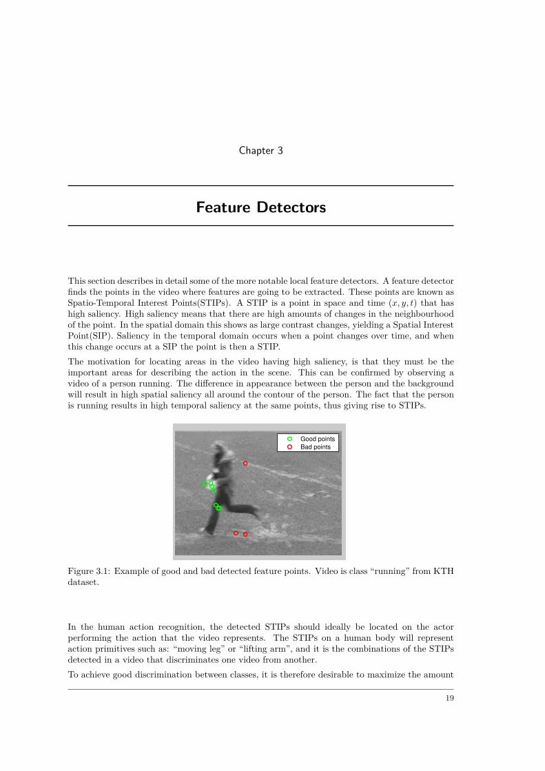
Figure 3.1: Example of good and bad detected feature points. Video is class “running” from KTHdataset.

In the human action recognition, the detected STIPs should ideally be located on the actorperforming the action that the video represents. The STIPs on a human body will representaction primitives such as: “moving leg” or “lifting arm”, and it is the combinations of the STIPsdetected in a video that discriminates one video from another.To achieve good discrimination between classes, it is therefore desirable to maximize the amount

19

CHAPTER 3. FEATURE DETECTORS

of good STIPs, i. e. STIPs on the actors, versus bad STIPs, i. e. STIPs on the background or onmotion that does not represent the action in the video. Figure 3.1 shows a frame of detectedSTIPs of “person running” from the KTH dataset. The detector has detected three points on thebackground, which will not add any useful information about the action.

3.1 Scale space

In the more challenging datasets, there can be large intraclass differences between videos. Videoshave different camera viewpoint, scene composition, resolution, etc. This results in that the sameobject, e. g. a human being, in one video can have the size of hundreds of pixels, while a humanin another video only takes up about 50 pixels of space. To be able to detect similar featuresin these videos, STIPs are detected in different temporal and spatial scales. These scales arerepresented as a convolution with a Gaussian blur function, where higher values of the variancesσ2, τ2, represents larger scales. This has intuitive meaning because the more the video is blurredthe more small details are lost, leaving only larger scale details behind. A video f(x, y, t) is thenrepresented by the scale-space

L(x, y, t;σ2, τ2) = f ∗ g(·;σ2l , τ

2l ) (3.1)

where g is the spatio-temporal Gaussian kernel

g(x, y, t;σ2l , τ

2l ) = exp(−(x2 + y2)/2σ2

l − t2/2τ2l )√

(2π)3σ4l τ

2l

(3.2)

having spatial variance σ2l and temporal variance τ2

l . Figure 3.2 shows the scale space of twodifferent videos from the same class: “Horse race”. In figure 3.2a, b and c the camera is close tothe race, while in 3.2d, e and f it is further away. This means that the number of features foundon the horse and rider will be larger, and represent smaller details in the close up video than theone with distance. Scale space representation can compensate for this as the blur removes thedetails. The features in 3.2c can then be comparable to the ones in 3.2d allowing the videos torepresent the same class even though their view point differs.

(a) Original (b) σ2l = 4 (c) σ2

l = 16

(d) Original (e) σ2l = 4 (f) σ2

l = 16

Figure 3.2: Parts of scale space representation of 2 videos from class: “Horse race” from UCF50.

20

3.2. HARRIS

There are multiple approaches to find the best points across scales. The trivial method is to applya multi-scale approach where the resulting points are the collection of all points from all scales.Another way is to try to estimate the best set of points across scales.

3.2 Harris

The Harris corner detector is a well-known algorithm for detection of salient regions in images[11]. The detector operates on a windowed second moment matrix

µ = g(·;σ2i ) ∗

(L2x LxLy

LxLy L2y

)(3.3)

where Lξ are derivatives of the image scale space

Lξ(x, y;σ2l ) = ∂L(x, y;σ2

l )∂ξ

(3.4)

and σi is the variance used in the gaussian kernel that serves as a window function. It is alsocalled the integration scale. The eigenvalues of µ determines if there is a corner, an edge or a“flat” area. If λ1 and λ2 both are large the point is a corner. If λ1 >> λ2 or λ2 >> λ1 the pointis an edge, and if both eigenvalues are small the area is “flat”.Since the computation of eigenvalues is expensive, the corners are detected as local maxima ofthe corner function

H = det(µ)− ktrace2(µ) = λ1λ2 − k(λ1 + λ2)2 (3.5)

3.3 Harris3D

Laptev [14] extended the idea of the Harris corner detector to three dimensions. The second-moment matrix is now spatio-temporal

µ = g(·;σ2i , τ

2i ) ∗

L2x LxLy LxLt

LxLy L2y LyLt

LxLt LyLt L2t

(3.6)

and the gaussian window function is now spatio-temporal having temporal variance τi. The cornerfunction becomes

H = det(µ)− ktrace3(µ) = λ1λ2λ3 − k(λ1 + λ2 + λ3)3 (3.7)

The implementation of the Laptev detector used in this thesis is the one provided on his webpagewhich also bundles the feature extractor for HOG/HOF features. The original algorithm [14]uses scale selection in space-time [17], but the newer implementation used in this thesis uses amulti-scale approach.

3.4 Cuboid detector

Dollar et al. [8] reports that the Harris3D detector in many cases does not detect enough featuresto perform well. The Cuboid detector is consequently tuned in a way that results in more STIPsthan Harris3D for the same videos. It is sensitive to periodic motions which occur often in actionvideos. The response function is

R = (f ∗ g(·, σ2l ) ∗ hev)2 + (f ∗ g(·, σ2

l ) ∗ hod)2 (3.8)

where hev and hod are the quadrature pair of one dimensional Gabor Filters, which are appliedtemporally and g is two dimensional Gaussian function applied spatially.

21

CHAPTER 3. FEATURE DETECTORS

3.5 Selective STIP

Selective STIP [3] tries to combine the best of existing approaches with a novel way of pointsuppression to strengthen the quality of detected STIPs. Instead of computing a response inspace and time simultaneously, the algorithm starts out with a simple detection of Spatial InterestPoints(SIPs) using Harris. For each interest point, an inhibition term is computed. The ideabehind the inhibition term is that points belonging to the background follow a particular geometricpattern. For this purpose, a gradient weight factor is introduced

∆Θ,σ(x, y, x− u, y − v) = |cos(Θσ(x, y)−Θσ(x− u, y − v))| (3.9)

where ∆Θ,σ(x, y) is the image gradient and u and v is the size of the mask. A suppression termis then defined as the weighted sum of gradient weights in the suppression surround of that point

tα(x, y) =∫ ∫

ΩCσ(x− u, y − v)×∆Θ,σ(x, y, x− u, y − v)dudv (3.10)

where Ω denotes the image coordinate domain. The resulting measure of corner strength, is thedifference between original Harris corner strength Cσ(x, y) and the suppression term

Cσ(x, y)− αtσ(x, y) (3.11)

where the factor α controls the amount of suppression.Scale selection is then applied to the remaining points in the same way as the original Harris3D[17],and the n best SIPs are kept as the final set of suppressed SIPs.The SIPs are then temporally constrained by point matching and Gabor filtering. The points arematched between two frames n and n − 1, and matching points are removed since static pointsdo not contribute to any motion information. The final points are selected based on the Gaborresponse at their locations. The resulting set of STIPs are usually sparser having a higher numberof STIPs on the actors in the scene.

3.6 Dense Sampling

Instead of detecting feature points, feature points can be sampled uniformly over the whole frameat every time instant in the video. The points are often distributed in a way the results in acertain amount of both spatial and temporal overlap to be sure to capture all the information inthe video. Dense sampling results in massive amounts of information and comes close to the rawpixel representation of the video. The amounts of bad features that dense sampling includes isoutweighed by the fact that it does not miss any information.

22

Chapter 4

Feature Descriptors

Feature descriptors represents the underlying pixels in a way that maximizes classification perfor-mance and gives a sparse representation. The descriptors should ideally be invariant to operationslike scale, rotation and illumination changes. This invariance enables descriptors to be matchedacross videos which have differences in these parameters.The descriptors are local, meaning that they are extracted in a predefined area around the detectedSTIPs. This area is often proportional to the scale where the STIP was detected. The descriptors

(a) Optical Flow (b) Gradient

Figure 4.1: Most significant optical flow and gradient and gradient vectors. Action is “handwav-ing” from KTH dataset.

are often based on gradients or optical flow, because these representations emphasize the parts inthe video where changes occur. Figure 4.1 shows an example of optical flow and spatial gradientsin a action video. The highest values are located on the actor, and the optical flow is concentratedaround the arms which makes sense because the action is “handwaving”.A popular way of constructing motion feature descriptors, is to extend an existing spatial featuredescriptor to account for the temporal domain as well. Histograms of Oriented Gradients(HOG) isone example of this. The 2D descriptor HOG is extended to 3D in two different ways: HOG/HOFand HOG3D.

23

CHAPTER 4. FEATURE DESCRIPTORS

4.1 Histograms of Oriented Gradients

Histograms of Oriented Gradients [5] is a popular 2D descriptor originally developed for persondetection. The important components of the detector are shown in figure 4.2. A HOG descriptoris computed using a block consisting of a grid of cells where each cell again consists of a grid ofpixels. The number of pixels in a cell and number of cells in a block can be varied. The structureperforming best according to the original paper is 3× 3 cells with 6× 6 pixels.

BlockCell

0 - 180

Gradient histogram

HOG Discriptor

Figure 4.2: Block diagram of HOG method.

For each cell in the block, a histogram of the gradients in the pixels is computed. The histogramhas 9 bins and a range of either 0-180or 0-360, where the former is known as unsigned and thelatter as signed. Each gradient votes for the bin corresponding to the gradient direction, with avote size corresponding to the gradient magnitude.Finally, each block is concatenated into a vector v and normalized by its L2 norm

vnorm = v√||v||22 + ε2

(4.1)

where ε is a small constant to prevent division by zero.The HOG descriptor is very similar to the descriptor used in SIFT [18]. The difference is thatthat the SIFT descriptor is rotated according to the orientation of the interest point.

4.2 HOG/HOF

HOG/HOF is the combination of histograms of oriented gradients with histograms of optical flow.HOF is computed the same way as HOG but with gradients replaced by optical flow. In [16],HOG is extended to include temporal information, by turning the 2D block in HOG into a 3Dvolume spanning (x, y, t). This volume is then divided into cuboids that corresponds to cells. Thesizes of the volume is determined by the detection scale

∆x,∆y = 2kσl∆t = 2kτl

24

4.3. HOG3D

making volumes larger for larger scales.

4.3 HOG3D

changes. We base our descriptor on gradient orientations, as those are robust to changesin illumination [6]. This also goes along with the works of Lowe [13] and Dalal et al. [3].

Laptev and Lindeberg [9] investigated single- and multi-scale N-jets, histograms ofoptical flow, and histograms of gradients as local descriptors for video sequences. Bestperformance has been obtained with optical flow and spatio-temporal gradients. Insteadof a direct quantization of the gradient orientations, however, each component of thegradient vector was quantized separately. In later work, Laptev et al. [10, 11] applieda coarse quantization to gradient orientations. However, as only spatial gradients havebeen used, histogram features based on optical flow were employed in order to capturethe temporal information. The computation of optical flow is rather expensive and resultsdepend on the choice of regularization method [1]. Therefore, we base our descriptor onpure spatio-temporal 3D gradients which are robust and cheap to compute. We performorientation quantization with up to 20 bins by using regular polyhedrons. Furthermore,we propose integral histograms for memory-efficient computation of features at arbitraryspatial and temporal scales.

An extension of the SIFT descriptor [13] to 3D was proposed by Scovanner et al. [17].For a given cuboid, spatio-temporal gradients are computed for each pixel. All pixels voteinto a Nx Ny Nt grid of histograms of oriented gradients. For orientation quantization,gradients are represented in polar coordinates f ,y that are divided into a 84 histogramby meridians and parallels. This leads to problems due to singularities at the poles sincebins get progressively smaller. We avoid the problem of singularities by employing reg-ular polyhedrons and use their homogeneously distributed faces as histogram bins. Ef-ficient histogram computation is then done by projecting gradient vectors onto the axesrunning through the center of the polyhedron and the face centers.

2 Spatio-temporal descriptorLocal descriptors are used to describe a local fragment in an image or a video. Usually,local regions are determined first by using an interest point detector or by dense sampling

Figure 1: Overview of the descriptor computation; (a) the support region around a pointof interest is divided into a grid of gradient orientation histograms; (b) each histogram iscomputed over a grid of mean gradients; (c) each gradient orientation is quantized usingregular polyhedrons; (d) each mean gradient is computed using integral videos.

Figure 4.3: HOG3D Block diagram. [13]

The former approach of using HOG as a spatio-temporal feature involved computing gradientsin cuboids instead of in cells, but the gradient directions are still two-dimensional. This makesthem unable to capture the temporal information in the video, which is why the addition of HOFsignificantly improves the results.HOG3D [13] changes the underlying approach by considering the three dimensional gradientinstead of the 2D gradient. The gradient is computed in three dimensions, and histograms arequantized into polyhedrons. This elegant way of quantization is intuitive if we look at the standardway of quantizing 2D gradient orientations by approximation of a circle with a polygon. Eachside of the polygon corresponds then to a histogram bin. By extending this to 3D the polygonbecomes a polyhedron. The polyhedron used is an icosahedron which has 20 sides, thus resultingin a 20 bin histogram of 3d gradient directions. The final descriptor is obtained by concatenationof histograms into a vector, and normalization by the L2 norm.

25

Chapter 5

Feature comparison

There are many different combinations of detector and descriptor that can be used in the frame-work, but which combination is the best? Wang et al. [35] tries to answer this question in a thor-ough comparison of detectors and descriptors. The detectors compared are: Harris3D, Cuboid,Hessian and Dense sampling. The descriptors used are HOG/HOF, HOG3D and ESURF. Alldifferent combinations of detector and descriptor are tested, to find the combination the yieldsthe highest precision. The testing framework used, is the same as described in section 2.4, wherethe videos are represented using bag-of-features and classified using a non-linear support vectormachine. Three different datasets are used: KTH, UCF sports and Hollywood2, to make surethat a results are not only achievable in a certain kind of videos.

5.1 Results

Table 5.1 shows the results for the KTH dataset. Harris3D is the best performing detector, andHOF is the best descriptor with the combination of the two gives the highest accuracy of 92.1%.The detectors outperform dense sampling in this dataset, and this could be explained by thesimplicity of the dataset. The lack of camera movement and background clutter makes it lesslikely for the detectors to detect STIPs on the background, while the dense sampling will alwaysinclude the background, which in KTH does not provide any valuable information about theaction.

HOG3D HOG/HOF HOG HOF Cuboids ESURFHarris3D 89.0% 91.8% 80.9% 92.1% - -Cuboids 90.0% 88.7% 82.3% 88.2% 89.1% -Hessian 84.6% 88.7% 77.7% 88.6% - 81.4%Dense 85.3% 86.1% 79.0% 88.0% - -

Table 5.1: Average accuracy for various detector/descriptor combinations on the KTH dataset.

Table 5.2 shows the results for UCF Sports. In this more complex dataset, dense sampling performsbetter than all of the detectors. This can be explained the amounts of contextual informationavailable in the background which is being captured by the dense sampling. In a sports dataset likeUCF, the different actions will often have very similar background, e. g. stadium, pool or indoorsports arena. Capturing these backgrounds can provide better accuracy. The best performingdescriptor is HOG3D and HOG/HOF the second-best.

27

CHAPTER 5. FEATURE COMPARISON

HOG3D HOG/HOF HOG HOF Cuboids ESURFHarris3D 79.7% 78.1% 71.4% 75.4% - -Cuboids 82.9% 77.7% 72.7% 76.7% 76.6% -Hessian 79.0% 79.3% 66.0% 75.3% - 77.3%Dense 85.6% 81.6% 77.4% 82.6% - -

Table 5.2: Average accuracy for various detector/descriptor combinations on the UCF Sportsdataset.

HOG3D HOG/HOF HOG HOF Cuboids ESURFHarris3D 43.7% 45.2% 32.8% 43.3% - -Cuboids 45.7% 46.2% 39.4% 42.9% 45.0% -Hessian 41.3% 46.0% 36.2% 43.0% - 77.3%Dense 45.3% 47.4% 39.4% 45.5 - -

Table 5.3: Average accuracy for various detector/descriptor combinations on the Hollywood2dataset.

The results for Hollywood2 is shown in table 5.3. This dataset is the most varied of the three, andthis is reflected in the results. Dense is again performing better than the detectors, but this timethe difference is not more than about 1% which could be explained by the fact that the intraclassvariance in background and context is higher in Hollywood2 than in UCF Sports.The best performing descriptor is HOG/HOF, and not HOG3D as in UCF Sports.It is hard to saywhy there is a difference between the performance of the descriptors across the different datasets,but some things can be concluded. Spatial Gradient information alone does not capture enoughinformation as HOG is consistently outperformed by the other descriptors.

5.2 Conclusion

In the two realistic datasets tested in this survey, dense sampling outperforms the detectors.The detectors only perform slightly better in KTH because of the simple scene and background.Feature detectors still needs a lot of improvement to truly capture the important information inthe video. Dense sampling does results in massive amounts of data, which can be time-consumingto process. Cuboids is generally the best performing of the detectors, but not significantly betterthan Harris3D.The descriptor performing best is varying across datasets, but in general it seems to the descrip-tors containing temporal information that yields the highest accuracy. HOG3D includes spatialinformation by considering the gradient direction in both space and time and HOF includes opti-cal flow which also encodes temporal changes in the video. HOG/HOF performs best in the mostcomplicated dataset: Hollywood2, and generally performs good in the other datasets as well.The combination selected for use in the experiments conducted in this thesis is Harris3D andHOG/HOF. This choice is made because it shows good results in all three datasets and althoughdense sampling gives a slightly better result in KTH and Hollywood, the more sparse representa-tion of STIPs is preferred. The implementation used [16] also has the advantage of bundling bothHarris3D and HOG/HOF.

28

Chapter 6

Representation

This section describes the representation of videos in the framework. The features extracted froma video have to be represented in a way that serves well for classification. This generally resultsin a dimensionality reduction were the video often ends up being represented as a single vector,which is a useful input to a classifier.

6.1 Bag-of-features

Bag-of-features is derived from the bag of words representation that is a used in natural languageprocessing to represent a text. The idea is that the text can be represented by the occurrencesof words, disregarding the order in which they appear in the text, or to use the metaphor in thename, put all the words in a bag and draw them out without knowing the order in which theywere put in. The result of the algorithm is a histogram of word occurrences, which can be moreuseful for comparing texts than a direct word-by-word comparison. The bins in the histogram arecalled the vocabulary, and can be the complete set of all kinds of words used in the text, or onlya subset as it might be relevant to filter out common words like: the, be, to and of.

200 400 600 800 1000

10

20

30

40

50

60

70

80

90

100

(a) Boxing 1200 400 600 800 1000

10

20

30

40

50

60

70

80

90

100

(b) Boxing 2200 400 600 800 1000

10

20

30

40

50

60

70

80

90

100

(c) Running

Figure 6.1: Three examples of word histograms from KTH with a vocabulary size of 1087 words.

The idea is extended to action recognition by Schuldt et al. [32]. Instead of a text, the histogram isnow representing a video and instead of words consisting of letters, they are now features extractedfrom the videos. The vocabulary has to be defined and is most often generated by clustering arepresentative subset of all features in a dataset as seen in figure 6.2. There is no final answer tothe number of words a vocabulary should consist of, but usually a more complex dataset requiresa larger vocabulary. The bag-of-features histogram is computed by putting each feature into thebin of the most similar word, most often measured by euclidean distance. Finally the histogram

29

CHAPTER 6. REPRESENTATION

is normalized so that all feature vectors are comparable, even if there is a different number offeatures in the videos. Figure 6.1 shows 3 examples of word histograms, where two are of thesame class. The histograms are not very meaningful to the human eye, and this lack of semanticmeaning is one of the downsides to the bag-of-features representation.

Input videos Vocabulary Word histograms

Figure 6.2: Bag-of-features representation.

Loosing the spatial and temporal information about the features is a strength and a weakness ofbag-of-features. It makes it possible to classify datasets that have high intraclass variance andby that nature high differences in the spatio-temporal collocation of features. Throwing away thelocation information does, on the other hand, cause classification problems as confusion betweensimilar classes.There are ways to change the feature representation before bag-of-features to maintain the colloca-tion information between the features. One example of this is a two step approach where featuresare grouped together based on their collocation to form new features. Yuan et al. [40] groupswords together as phrases, where each phrase represents a combination of words. Chakrabortyet al. [3] uses a pyramid division of features that divides them into groups based on their spatiallocation.

30

Chapter 7

Supervised Learning

Supervised learning uses training data to train a classifier that encodes the differences betweenthe classes. The training data are supervised, i. e. the labels of the samples are known, so theclassifier can learn the relationship between the features and the labels. Most of supervisedclassifiers requires significant amounts of training data, depending on the number of classes andthe complexity of the dataset.One challenge is not to overfit the classifier to the training data, resulting in that the classifieris only able to perform well on data very similar to the training data. In the opposite case,underfitting can cause the classifier to become too general, and the accuracy will suffer.

7.1 Support Vector Machine

A Support Vector Machine(SVM) is a linear binary classifier that seeks to maximize the distancebetween the points of two classes. The solution consists of a hyperplane that separates thetwo classes in the best way. It is possible to extend the SVM to achieve non-linear multi-classclassification.

Decision hyperplane

Margin

Support vectors

Figure 7.1: Support Vector Machine

31

CHAPTER 7. SUPERVISED LEARNING

7.1.1 Linear separable classesIn the simple case in fig 7.1, it is actually possible to obtain complete separation between twoclasses using a linear function. When the space is extended from two dimensions to n dimensionsthis linear function becomes a hyperplane. Many different hyperplanes could separate the points,but the desired hyperplane is the one in middle between the two point clouds, i. e. it maximizesthe distance to the points. The points that influences the position of the hyperplane are the pointsclosest to the empty space between the classes. These points are called support vectors.The distance between the hyperplane and the support vectors is the margin, so the desired hy-perplane is defined as the hyperplane that maximizes the margin.We have L training points, where each input xi is a D-dimensional feature vector, and is one oftwo classes yi ∈ −1,+1. The hyperplane is defined as

w · x+ b = 0 (7.1)

where w is the normal to the hyperplane. The objective of the SVM can then be described asfinding w and b such that the two classes are separated

xi · w + b ≥ +1 for yi = +1 (7.2)xi · w + b ≤ −1 for yi = −1 (7.3)

These equations can be combined into

yi(xi · w + b)− 1 ≥ 0 ∀i (7.4)

The objective is to maximize the margin, which by simple vector geometry is found to be 1||w|| .

This means that the optimization problem can be formulated as a minimization of ||w|| or rather

minimize 12 ||w||

2

subject to yi(xi · w + b)− 1 ≥ 0 ∀i(7.5)

as this makes it possible to perform quadratic programming optimization later on. By introducingLagrange multipliers α, the dual problem can eventually be reached

maximizeα

L∑i=1

αi −12α

THα

subject to αi ≥ 0 ∀i,L∑i=1

αiyi = 0

(7.6)

This problem is solved using a quadratic programming solver, yielding a solution for α and therebyw and b. Points can now be classified using the decision function

y′ = sgn(w · x′ + b) (7.7)

7.1.2 Non-separable pointsIn the formulation used above, it is assumed that the two classes are completely separable by ahyperplane, but this is often not the case. The points are often entangled in a way that makes itimpossible to separate them, but it is still desired to have a classifier that makes as few mistakesas possible.This is achieved by introducing a positive slack variable ξi, i = 1 . . . L. This slack allows the points

32

7.1. SUPPORT VECTOR MACHINE

to be located on the “wrong” side of the hyperplane as seen in the modified expressions

xi · w+b ≥ +1− ξi for yi = +1 (7.8)xi · w+b ≤ −1 + ξi for yi = −1 (7.9)

ξi ≥ 0∀i (7.10)

The minimization problem is reformulated as

minimize 12 ||w||

2 + C

L∑i=1

ξi

subject to yi(xi · w + b)− 1 + ξi ≥ 0 ∀i

(7.11)

where the parameter C controls how much the slack variables are punished.

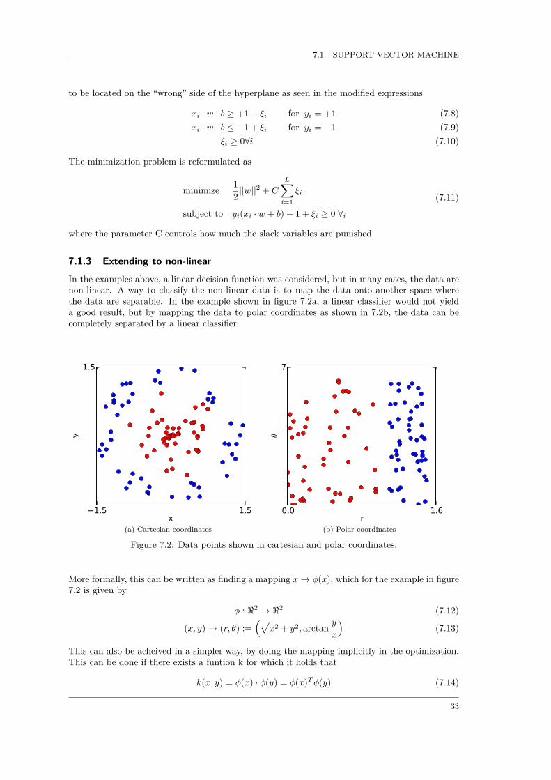
7.1.3 Extending to non-linear

In the examples above, a linear decision function was considered, but in many cases, the data arenon-linear. A way to classify the non-linear data is to map the data onto another space wherethe data are separable. In the example shown in figure 7.2a, a linear classifier would not yielda good result, but by mapping the data to polar coordinates as shown in 7.2b, the data can becompletely separated by a linear classifier.

1.5 1.5x

1.5

y

(a) Cartesian coordinates

0.0 1.6r

7

θ

(b) Polar coordinates

Figure 7.2: Data points shown in cartesian and polar coordinates.

More formally, this can be written as finding a mapping x→ φ(x), which for the example in figure7.2 is given by

φ : <2 → <2 (7.12)

(x, y)→ (r, θ) :=(√

x2 + y2, arctan yx

)(7.13)

This can also be acheived in a simpler way, by doing the mapping implicitly in the optimization.This can be done if there exists a funtion k for which it holds that

k(x, y) = φ(x) · φ(y) = φ(x)Tφ(y) (7.14)

33

CHAPTER 7. SUPERVISED LEARNING

i. e. k is equal to the dot product of the vectors. K is called a kernel-function, and it enables theproblem to be solved in complexity of the original space, while having the classification accuracyof the potentialy higher-order space.

Kernel ExpressionLinear k(x, y) = xT y + c

Polynomial k(x, y) =(axT y + c

)dRadial basis function(RBF) k(x, y) = exp

(− ||x−y||

2

2σ2

)Intersection k(x, y) =

n∑i=1

min(xi, yi)

χ-squared k(x, y) = 1−n∑i=1

(xi−yi)2

12 (xi+yi)

Table 7.1: Different examples of kernel functions.

Table 7.1 shows some popular choices of SVM kernels. The intersection and χ-squared kernelsare especially useful when it comes to bag-of-features classification because they provide a goodway to capture the difference between histograms which is the common way to represent a videoin bag-of-features.

7.1.4 Multi-class approachThe above-mentioned SVM classifiers have all considered the binary case of labelling a video aseither one class or the other, but this can of course be extended to the general case of n classes.Two common approaches are: one-vs-all and one-vs-one.In one-vs-all, each classifier is trained using training data from one class, vs. the training datafrom all other classes resulting in n classifiers for n classes. In classification, a point is assigned toclass that has the highest output of the descision function. The classifiers have to be trained in away that results in the same range of their output to make the descision functions comparable.In one-vs-one a classifier is constructed for each combination of two classes which results inn(n − 1)/2 classifiers. In the classification step, each point casts a vote for one of the classes ineach of the classifiers and in the end picks the class having the highest number of votes. In theevent of a tie, the class being assigned is usually arbitrary.The implementation used in this work, libSVM[4], uses one-vs-one for multi-class approach.

34

Chapter 8

Unsupervised Learning

In unsupervised Learning, there is no prior knowledge of labels or constraints between the data,and it is up to the algorithm to cluster the videos based on their features. This clustering canhave a fixed goal of a number of clusters, or the number can be variable making it part of theproblem to figure out how many clusters to choose.One question is how to evaluate the results of an unsupervised algorithm. If the results has acluster that consists of 4 videos, where 2 videos are of class a and 2 of class b, is this evaluatedas 2 positive results for class a and 2 negative for class b, or the opposite? When there are nosupervised data involved, a cluster does not have a prior label, and if the algorithm does notoutput a fixed number of clusters, there can be more than one cluster per label.It could also be the case, that class a and b are actually similar in a way different from the problemformulation. If e. g. class a is running, class b is boxing, but all videos in the cluster takes place ina baseball stadium, the cluster could be representing baseball stadium and not running or boxing.When the features used have no specific semantic meaning, the clusters found by an unsupervisedmethod can not be guaranteed to have the semantic meaning defined by the prior class definitions.

8.1 K-means clustering

K-meas clustering is a clustering method that divides n points into k clusters, where each clusterbelongs to a mean value of the cluster. Formally this is defined as minimizing the sum of squareswithin each cluster

argminS

k∑i=1

∑xj∈Si

||xj − µi||2 (8.1)

where xj is a point and µi is the mean belonging to cluster i. Solving this problem is NP-hard,but there are efficient heuristic algorithms to reach an approximation.

8.1.1 Standard algorithm

1. InitializationThe algorithm is usually initialized by setting all the means to a random value, but thereare also various heuristics that can choose starting means based on the data.

2. Assignment stepIn the assignment step, each point is assigned to the nearest mean based on the distancebetween the point and the means

Si = xp : ||xp − µi|| ≤ ||xp − µj || ∀ j = 1 . . . k (8.2)

35

CHAPTER 8. UNSUPERVISED LEARNING

This distance is usually the euclidean distance, but other distance measures can be used.When each point has been assigned to one mean, the result is k temporary clusters.

3. Update stepA new mean is calculated in each cluster as the centroid of all the points in the cluster, i. e.the average of the point coordinates in a cluster.

µi = 1|Si|

∑xj∈Si

xj (8.3)

4. Repeat step 2 and 3 until convergence.

The algorithm is simple and efficient, but it also has a number of drawbacks. The solution foundwill almost always only be a local minimum. Picking the best out of multiple runs with differentinitializations is a way of improving the solution, but a guaranteed global minimum can of coursenot be found.K-means has a tendency to find clusters that are similar in size. This does not make it suitablefor data where there are significant differences in the sizes of the clusters.Because that the distance measure used is the euclidean distance, the result is spherical clusterswhich is not very well suited for certain distributions.

8.2 Affinity Propagation

Affinity Propagation [10] is a message passing algorithm. This means that each point in theclustering exchanges messages with all other points to gain an understanding of the compositionof the data. The result of affinity propagation is a number of exemplars, which are points selectedfrom the input points. Each cluster has exactly one exemplar, which can be seen as the point thebest represents the points in the cluster. Because there can be only one exemplar in a cluster,and every point has to choose an exemplar, each exemplar is its own exemplar. The number of

(a) Responsibilities (b) Availabilities

Figure 8.1: The two types of messages exchanged in affinity propagation. [10]

exemplars are not constrained to a fixed number like in e. g. k-means. Instead each point has anumber called the preference p(i). Points having a higher preference are more likely to becomeexemplars. The preference is usually equal for all points, and the author suggest setting it to themedian of the similarities. When collective preferences determine the number of resulting clusters.Exemplars are selected based on the messages which are passed between the points. The inputto the algorithm are pairwise similarities between all the points s(i, k). Any similarity measure

36

8.2. AFFINITY PROPAGATION

can be used, and similarities do not have to be symmetric: i. e. s(i, k) = s(k, i) is always true, orsatisfy the triangle equality: s(i, k) < s(i, j) + s(j, k).There are two types of messages that are being exchanged between the points: responsibility andavailability, as shown in figure 8.1. Responsibility r(i, k), sent from point i to candidate exemplarpoint k, is the evidence of how much i wants k to be it’s exemplar. This evidence is based on howi views its other options of exemplars.Availability a(i, k), sent from candidate exemplar point k to i, is the evidence of how much kthinks that it should be i’s exemplar. The availability from k is based on the responsibilities sentto k, i. e. if other points like k as an exemplar, k must be a good candidate exemplar and will thensend a higher availability to i.

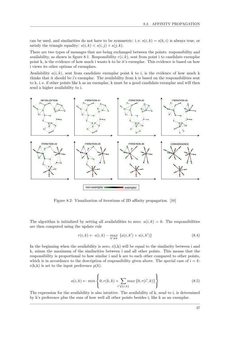
Figure 8.2: Visualization of iterations of 2D affinity propagation. [10]

The algorithm is initialized by setting all availabilities to zero: a(i, k) = 0. The responsibilitiesare then computed using the update rule

r(i, k)← s(i, k)−maxk′ 6=k

a(i, k′) + s(i, k′) (8.4)

In the beginning when the availability is zero, r(i,k) will be equal to the similarity between i andk, minus the maximum of the similarities between i and all other points. This means that theresponsibility is proportional to how similar i and k are to each other compared to other points,which is in accordance to the description of responsibility given above. The special case of i = k:r(k,k) is set to the input preference p(k).

a(i, k)← min

0, r(k, k) +∑

i′ /∈i,k

max 0, r(i′, k)

(8.5)

The expression for the availability is also intuitive. The availability of k, send to i, is determinedby k’s preference plus the sum of how well all other points besides i, like k as an exemplar.

37

CHAPTER 8. UNSUPERVISED LEARNING

The self-availability a(k, k) is a measure of the accumulated evidence that k is an exemplar andis computed differently

a(k, k)←∑i′ 6=k

max 0, r(i′, k) (8.6)

For each iteration of computing availabilities and responsibilities, the temporary exemplars aredetermined by

exemplar(i) = argmaxk

a(i, k) + r(i, k) (8.7)

which means that if k = i, i is itself an exemplar, and else k is the exemplar of i. When theexemplar choices does not change for a number of iterations, convergence is reached and thealgorithm terminates.Figure 8.2 shows an illustration of the different iterations of affinity propagation. The messagesstarts out being almost equal between all points, but as the number of iterations increase themessages to some points increases and finally the algorithm converges with three exemplars.

38

Chapter 9

Results

This chapter presents the experimental results and comparison of the chosen subset of methodsdescribed in the previous sections. Section 9.1 describes the algorithms and parameters used inthe tests. In section 9.2, the supervised results are presented for each of the datasets: KTHand UCF50. The results from the unsupervised algorithms are presented in section 9.3, anda comparison of supervised and unsupervised algorithms is given. Finally the parameters forbag-of-features vocabulary generation are evaluated.

9.1 Experimental Setup

The framework used in all experiments is the one described in section 2.4. The two first steps inthe framework: feature detector and feature descriptor are fixed in all the experiments, while thelast two: video representation and classification are changed, to compare the results.The feature detector used is Harris3D which is combined with the HOG/HOF descriptor. Theimplementation used is the updated version of the one described in [16], obtained from the authorsweb page. The default settings are used for parameters like number of temporal and spatial scalesand detector sensitivity. SVM is used for supervised classification and affinity propagation andk-means clustering are used for unsupervised classification.For each of the datasets, a number of different vocabularies are built to find the best strategy forvocabulary generation. Each individual experiment utilizes the vocabulary that provides the bestresult for that specific experiment.The measure used for comparison is mean average precision. Average precision is the average ofall true positive percentages across classes. When cross validation is used, the test is run multipletimes resulting in different average precisions. The mean of all these runs is reported as the resultof the cross validation.

9.2 Supervised

This section presents the results of the supervised classifier. The classifier used is a support vectormachine(SVM) and the implementation used is libsvm [4], with a χ-squared kernel. Becauselibsvm does not have native support for the χ-squared kernel, the kernel is precomputed usingan external function. The default option of one-vs-one approach for multi-class classification isselected.

39

CHAPTER 9. RESULTS

9.2.1 KTHThe 600 videos in KTH are partitioned according to the directions given in the dataset [32], withone exception: the video files are not split up into the sequences described in the directions, butkept together meaning that one video file contains the same subject performing an action multipletimes. This does not seem to affect the recognition rate particularly, even when compared to Wanget al. [35], where the mirrored versions of the clips also are used to gain more data.Figure 9.1 shows the confusion matrix for the result of the SVM classification of KTH. Theaverage precision of 89.4% is close to the precision of 91.8% reported by [35], even though thereare differences in methodology.

.94 .06

.03 .97

.19 .11 .69

.92 .08

.17 .83

1.0

boxing

handclapping

handwaving

jogging

running

walking

boxing

handclapping

handwaving

jogging

running

walking

Figure 9.1: Confusion matrix of the best SVM classification of the KTH dataset. Avg. precision:89.4%

There is some confusion among the arm classes and among the leg classes but not between thetwo. This is expected, as a video involving movement of the arms should be more likely to beconfused with a class the involves arm movement. The highest error is found in handwaving,which is confused as boxing almost 20% of the time.

9.2.2 UCF50UCF50 is classified using 10-fold cross-validation, i. e. the videos are divided into 10 groups andfor each test run the classifier is trained using 1 group and tested on 9 remaining groups. Thereported precision and confusion matrix is the average over the 10 runs.Figure 9.2 shows the confusion matrix for the best SVM classification. There are large differencesbetween the precision of the different classes, ranging from 98% in class 5: “Billiards” to 0% inclass 44: “TaiChi”. Class 45: “TennisSwing” has many false positives from other classes.

9.3 Unsupervised

The unsupervised algorithms use the same word histograms for input as the SVM. K-means usesthe histograms directly while affinity propagation uses their pairwise χ-squared distances. The

40

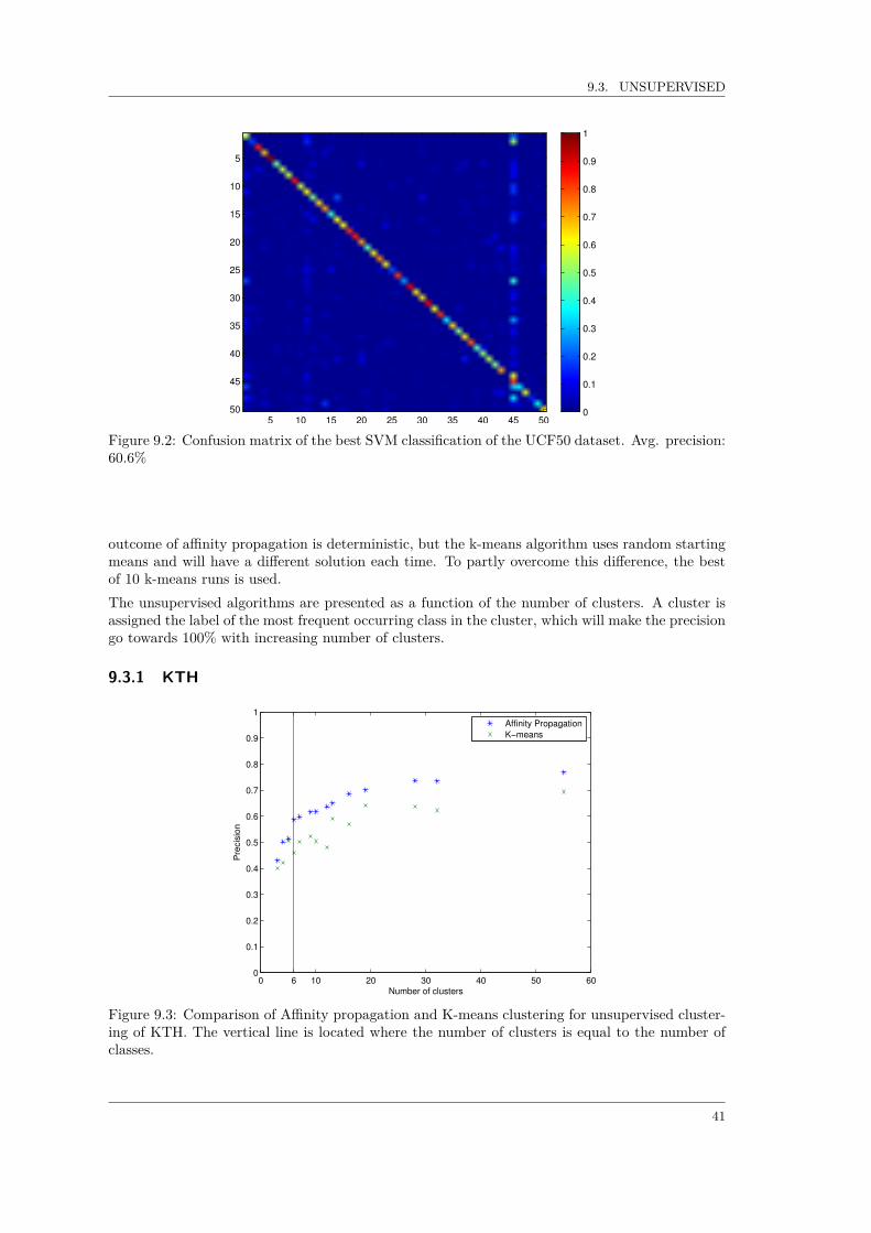
9.3. UNSUPERVISED

5 10 15 20 25 30 35 40 45 50

5

10

15

20

25

30

35

40

45

50 0

0.1

0.2

0.3

0.4

0.5

0.6

0.7

0.8

0.9

1

Figure 9.2: Confusion matrix of the best SVM classification of the UCF50 dataset. Avg. precision:60.6%

outcome of affinity propagation is deterministic, but the k-means algorithm uses random startingmeans and will have a different solution each time. To partly overcome this difference, the bestof 10 k-means runs is used.The unsupervised algorithms are presented as a function of the number of clusters. A cluster isassigned the label of the most frequent occurring class in the cluster, which will make the precisiongo towards 100% with increasing number of clusters.

9.3.1 KTH

0 6 10 20 30 40 50 600

0.1

0.2

0.3

0.4

0.5

0.6

0.7

0.8

0.9

1

Number of clusters

Pre

cis

ion

Affinity Propagation

K−means

Figure 9.3: Comparison of Affinity propagation and K-means clustering for unsupervised cluster-ing of KTH. The vertical line is located where the number of clusters is equal to the number ofclasses.

41

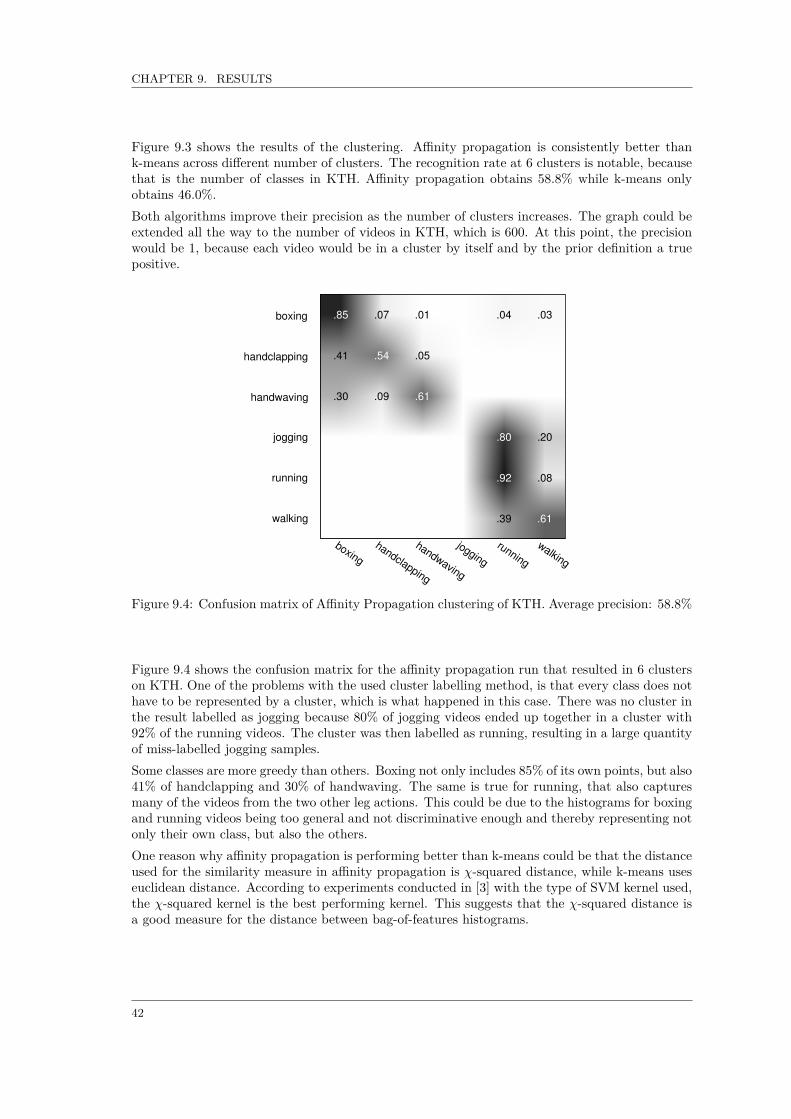
CHAPTER 9. RESULTS

Figure 9.3 shows the results of the clustering. Affinity propagation is consistently better thank-means across different number of clusters. The recognition rate at 6 clusters is notable, becausethat is the number of classes in KTH. Affinity propagation obtains 58.8% while k-means onlyobtains 46.0%.Both algorithms improve their precision as the number of clusters increases. The graph could beextended all the way to the number of videos in KTH, which is 600. At this point, the precisionwould be 1, because each video would be in a cluster by itself and by the prior definition a truepositive.

.85 .07 .01 .04 .03

.41 .54 .05

.30 .09 .61

.80 .20

.92 .08

.39 .61

boxing

handclapping

handwaving

jogging

running

walking

boxing

handclapping

handwaving

jogging

running

walking

Figure 9.4: Confusion matrix of Affinity Propagation clustering of KTH. Average precision: 58.8%

Figure 9.4 shows the confusion matrix for the affinity propagation run that resulted in 6 clusterson KTH. One of the problems with the used cluster labelling method, is that every class does nothave to be represented by a cluster, which is what happened in this case. There was no cluster inthe result labelled as jogging because 80% of jogging videos ended up together in a cluster with92% of the running videos. The cluster was then labelled as running, resulting in a large quantityof miss-labelled jogging samples.Some classes are more greedy than others. Boxing not only includes 85% of its own points, but also41% of handclapping and 30% of handwaving. The same is true for running, that also capturesmany of the videos from the two other leg actions. This could be due to the histograms for boxingand running videos being too general and not discriminative enough and thereby representing notonly their own class, but also the others.One reason why affinity propagation is performing better than k-means could be that the distanceused for the similarity measure in affinity propagation is χ-squared distance, while k-means useseuclidean distance. According to experiments conducted in [3] with the type of SVM kernel used,the χ-squared kernel is the best performing kernel. This suggests that the χ-squared distance isa good measure for the distance between bag-of-features histograms.

42

9.3. UNSUPERVISED

0 10 20 30 40 50 60 70 80 900

0.05

0.1

0.15

0.2

0.25

0.3

Number of clusters

Pre

cis

ion

Affinity Propagation

K−means

Figure 9.5: Comparison of affinity propagation and K-means clustering for unsupervised clusteringof UCF50. The vertical line is located where the number of clusters is equal to the number ofclasses.

9.3.2 UCF50

The unsupervised results for UCF50 are seen in figure 9.5. Affinity propagation performs betterthan k-means over all number of clusters, and obtains a precision of 18.0% at 50 clusters. Thegap between AP and k-means is smaller than it is for KTH.

5 10 15 20 25 30 35 40 45 50

5

10

15

20

25

30

35

40

45

50 0

0.1

0.2

0.3

0.4

0.5

0.6

0.7

0.8

0.9

1

Figure 9.6: Confusion matrix of affinity propagation clustering of UCF50. Average precision:18.9%

Figure 9.6 shows the confusion matrix for the best affinity propagation result. There is significantconfusion, what mostly seems random, in almost every class apart from a few exceptions. Classes:33: “Punch”, 14: “HorseRiding” and 19: “JumpingJack”, are the three classes having the highest

43

CHAPTER 9. RESULTS

precision. Class 1:“BaseballPitch” and 45: “TennisSwing” are attracting many false positives frommany other classes.

9.4 Comparison of supervised and unsupervised

This section compares the precision of the SVM classification with the precision of the unsuper-vised algorithms.

SVM AP K-meansKTH 89.4% 58.8% 46.0%

UCF50 50% 18.9% 14.8%

Table 9.1: Comparison of average precision of supervised and unsupervised algorithms.

Table 9.1 shows the average precisions from supervised and unsupervised classification. Theunsupervised precisions used, are from the clustering runs that has number of clusters equal tothe number of classes, so that the results are comparable. SVM classification is over 30% moreprecise in KTH, and more than double as precise for UCF50 compared to affinity propagation.

9.5 Vocabulary Building Strategy

Number of words1078 2160 4856

AP 20.000 87.0% 85.6% 87.0%KM 20.000 88.4% 82.4% 87.9%KM 50.000 84.2% 85.6% 89.4%KM 100.000 88.4% 85.6% 88.4%

Table 9.2: Comparison of different parameters for vocabulary building for KTH. AP is affinitypropagation and KM is K-means.

The vocabulary is an important part of the bag-of-features framework. This makes it interestingto explore the different parameters used for vocabulary building to see which values that yieldsthe best performance. The vocabulary is the result of clustering where the input is a sampleof features from the dataset. Affinity propagation and k-means are compared to see if the usedclustering algorithm makes any difference.Three different vocabulary sizes are tested for each dataset. Affinity propagation does not outputa fixed number of clusters, so by trying different p values, 3 different number of words were foundfor each dataset. The number of words output by AP is then used as the input k to k-means toget a comparable number of clusters. The number of input samples to the clustering algorithmsused are: 20,000, 50,000 and 100,000. To get a representative sample from the set of all features,the same number of random features is sampled from each of the videos in the dataset to formthe collective set used for clustering. This is only done for k-means because the implementationof AP has too high complexity in memory for running on large sample sizes, at least for thecomputational power available in this project.The different vocabularies have been tested only using the supervised algorithm.Table 9.2 shows the results for KTH. There are not a huge difference between the different strate-gies. K-means and AP perform similarly on 20.000 input features. There is a little gain in

44

9.5. VOCABULARY BUILDING STRATEGY

Number of words591 2839 4327

AP 20,000 50.4% 55.7% 58.3%KM 20,000 49.5% 56.4% 58.4%KM 50,000 51.2% 54.4% 59.3KM 100,000 51.1% 57.9% 60.6%

Table 9.3: Comparison of different parameters for vocabulary building for UCF50. AP is affinitypropagation and KM is K-means.

performance by using more input points. K-means with 50.000 points performs better than k-means with 100.000 for the highest number of words, but this could be explained by the inherentrandom outcome of k-means.Table 9.3 shows the results for UCF50. Here, the performance increases significantly with thenumber of words, which is not surprising as a diverse dataset is expected to require a diversevocabulary to represent it. The performance also increases a little with the number of inputsamples, but not as much as expected.

45

Chapter 10

Conclusion

This thesis has explored the pros and cons of methods within the bag-of-features framework. Thebest methods within each component category were compared, and a few combinations selectedfor experimental tests. The Harris3D detector with HOG/HOF descriptor was used in a bag-of-features representation as a base for classification. Supervised and unsupervised classifiers werecompared on the simple KTH dataset and the more complicated UCF50 dataset.The results of the supervised SVM classification was an average precision of 89.4% in KTH. Thiswas expected as this is simillar to what others achieved on KTH. This shows that KTH is gettingto simple for comparison of state-of-the art supervised algorithms, as there is not enough roomfor future improvement. The mean average precision for SVM classification of UCF50 was 60.6%in UCF50, with many higly varying performance of the different classes.The two unsupervised algorithms tested were: affinity propagation(AP) and k-means. Affinitypropagation outperforms k-means for both KTH and UCF50, but the difference is more significantin KTH, which could mean that affinity propagation works better for small problems. The averageprecision of affinity propagation is 60% for KTH and 18.9% for UCF50.One of the goals of this thesis was to compare supervised and unsupervised classification. SVMoutperforms AP by about 30% in KTH and 20% in UCF50. The training data used in SVMprovides a lot of information that the unsupervised methods do not have. UCF50 is especially aproblem for the unsupervised algorithms. Even though the unsupervised algorithms do not achievethe best performance, they obtained their results without the use of training data which is a hugeadvantage. Further development of unsupervised methods will make classification less dependantof large amounts of training data. Semisupervised methods are also gaining attentention for theirability to combine the advantages of supervised and unsupervised algorithms.Two different algorithms were tested for vocabulary building: affinity propagation and k-means.The clustering was done with a different number of words and a different number of input featuresto see which combination that yielded the best performance for supervised classification. Theaverage precision of the SVM increases with the number of words in the vocabulary, having thebest vocabulary at 4856 words in KTH and 4327 in UCF50. One explanation could be thatSVM is good at dealing with many-dimensional points, and therefore benefits from having theextra information provided by a larger vocabulary. Affinity propagation does not seem to provideany advantage over k-means for vocabulary building as the two algorithms have almost the sameprecision in the comparable case of 20,000 input samples. Increasing the number of sampledfeatures for clustering does not improve the vocabulary much above 50.000 features. The numberof samples is more important for UCF50 than for KTH which can be expected because UCF50 isa much more diverse dataset.

47

Bibliography

[1] Moshe Blank, Lena Gorelick, Eli Shechtman, Michal Irani, and Ronen Basri. Actions as space-time shapes. In The Tenth IEEE International Conference on Computer Vision (ICCV’05),pages 1395–1402, 2005.

[2] A.F. Bobick and J.W. Davis. The recognition of human movement using temporal templates.Pattern Analysis and Machine Intelligence, IEEE Transactions on, 23(3):257–267, 2001.

[3] B. Chakraborty, M.B. Holte, T.B. Moeslund, and J. Gonzalez. Selective spatio-temporalinterest points. Computer Vision and Image Understanding, 2011.

[4] Chih-Chung Chang and Chih-Jen Lin. LIBSVM: A library for support vector machines. ACMTransactions on Intelligent Systems and Technology, 2:27:1–27:27, 2011. Software availableat http://www.csie.ntu.edu.tw/˜cjlin/libsvm.

[5] N. Dalal and B. Triggs. Histograms of oriented gradients for human detection. In ComputerVision and Pattern Recognition, 2005. CVPR 2005. IEEE Computer Society Conference on,volume 1, pages 886–893. Ieee, 2005.

[6] S. Danafar and N. Gheissari. Action recognition for surveillance applications using optic flowand svm. In Proceedings of the 8th Asian conference on Computer vision-Volume Part II,pages 457–466. Springer-Verlag, 2007.

[7] V. Delaitre, I. Laptev, and J. Sivic. Recognizing human actions in still images: a study ofbag-of-features and part-based representations. IEEE PAMI, 31(10):1775–1789, 2009.

[8] P. Dollar, V. Rabaud, G. Cottrell, and S. Belongie. Behavior recognition via sparse spatio-temporal features. In Visual Surveillance and Performance Evaluation of Tracking andSurveillance, 2005. 2nd Joint IEEE International Workshop on, pages 65–72. IEEE, 2005.

[9] D. Dueck and B.J. Frey. Non-metric affinity propagation for unsupervised image categoriza-tion. In Computer Vision, 2007. ICCV 2007. IEEE 11th International Conference on, pages1–8. IEEE, 2007.

[10] Brendan J. Frey and Delbert Dueck. Clustering by passing messages between data points.Science, 315:972–976, 2007. URL www.psi.toronto.edu/affinitypropagation.

[11] C. Harris and M. Stephens. A combined corner and edge detector. In Alvey vision conference,volume 15, page 50. Manchester, UK, 1988.

[12] G. Johansson. Visual perception of biological motion and a model for its analysis. Attention,Perception, & Psychophysics, 14(2):201–211, 1973.

[13] Alexander Klaser, Marcin Marsza lek, and Cordelia Schmid. A spatio-temporal descriptorbased on 3d-gradients. In British Machine Vision Conference, pages 995–1004, 2008.

49

BIBLIOGRAPHY

[14] I. Laptev. On space-time interest points. International Journal of Computer Vision, 64(2):107–123, 2005.

[15] I. Laptev, B. Caputo, C. Schuldt, and T. Lindeberg. Local velocity-adapted motion eventsfor spatio-temporal recognition. Computer Vision and Image Understanding, 108(3):207–229,2007.

[16] I. Laptev, M. Marszalek, C. Schmid, and B. Rozenfeld. Learning realistic human actions frommovies. In Computer Vision and Pattern Recognition, 2008. CVPR 2008. IEEE Conferenceon, pages 1–8. IEEE, 2008.

[17] T. Lindeberg. Feature detection with automatic scale selection. International journal ofcomputer vision, 30(2):79–116, 1998.

[18] D.G. Lowe. Distinctive image features from scale-invariant keypoints. International journalof computer vision, 60(2):91–110, 2004.

[19] D. Marr and H.K. Nishihara. Representation and recognition of the spatial organization ofthree-dimensional shapes. Proceedings of the Royal Society of London. Series B. BiologicalSciences, 200(1140):269–294, 1978.

[20] M. Marszalek, I. Laptev, and C. Schmid. Actions in context. In Computer Vision and PatternRecognition, 2009. CVPR 2009. IEEE Conference on, pages 2929–2936. IEEE, 2009.

[21] Microsoft. Kinect for xbox 360, 2012. URL http://www.xbox.com/da-DK/Kinect.

[22] Thomas B. Moeslund and Erik Granum. A survey of computer vision-based human motioncapture. Computer Vision and Image Understanding, 81(3):231 – 268, 2001.

[23] Thomas B. Moeslund, Adrian Hilton, and Volker Kruger. A survey of advances in vision-based human motion capture and analysis. Computer Vision and Image Understanding, 104(2–3):90–126, 2006.

[24] J.C. Niebles, H. Wang, and L. Fei-Fei. Unsupervised learning of human action categories usingspatial-temporal words. International Journal of Computer Vision, 79(3):299–318, 2008.

[25] University of Central Florida. Ucf50 dataset. URL http://vision.eecs.ucf.edu/datasetsActions.html.

[26] University of Minnesota. Unusual crowd activity dataset. URL http://mha.cs.umn.edu/proj_events.shtml.

[27] R. Poppe. A survey on vision-based human action recognition. Image and Vision Computing,28(6):976–990, 2010.

[28] D.K. Ramanan and D. Forsyth. Automatic annotation of everyday movements. ComputerScience Division, University of California, 2003.

[29] K. Rapantzikos, Y. Avrithis, and S. Kollias. Spatiotemporal saliency for event detectionand representation in the 3d wavelet domain: potential in human action recognition. InProceedings of the 6th ACM international conference on Image and video retrieval, pages294–301. ACM, 2007.

[30] C. Rosenberg, M. Hebert, and H. Schneiderman. Semi-supervised self-training of objectdetection models. 2005.

[31] S. Savarese, A. DelPozo, J.C. Niebles, and L. Fei-Fei. Spatial-temporal correlatons for un-supervised action classification. In Motion and video Computing, 2008. WMVC 2008. IEEEWorkshop on, pages 1–8. IEEE, 2008.

50

BIBLIOGRAPHY

[32] C. Schuldt, I. Laptev, and B. Caputo. Recognizing human actions: A local svm approach.In Pattern Recognition, 2004. ICPR 2004. Proceedings of the 17th International Conferenceon, volume 3, pages 32–36. IEEE, 2004.

[33] P. Scovanner, S. Ali, and M. Shah. A 3-dimensional sift descriptor and its application toaction recognition. In Proceedings of the 15th international conference on Multimedia, pages357–360. ACM, 2007.

[34] N. Shental, A. Bar-Hillel, T. Hertz, and D. Weinshall. Computing gaussian mixture modelswith em using equivalence constraints. Advances in neural information processing systems,16:465–472, 2004.

[35] H. Wang, M.M. Ullah, A. Klaser, I. Laptev, C. Schmid, et al. Evaluation of local spatio-temporal features for action recognition. BMVC, 2009.

[36] S. Wang, Z. Liu, S. Lv, Y. Lv, G. Wu, P. Peng, F. Chen, and X. Wang. A natural visibleand infrared facial expression database for expression recognition and emotion inference.Multimedia, IEEE Transactions on, 12(7):682–691, 2010.

[37] D. Weinland, R. Ronfard, and E. Boyer. A survey of vision-based methods for action rep-resentation, segmentation and recognition. Computer Vision and Image Understanding, 115(2):224–241, 2011.

[38] G. Willems, T. Tuytelaars, and L. Van Gool. An efficient dense and scale-invariant spatio-temporal interest point detector. Computer Vision–ECCV 2008, pages 650–663, 2008.

[39] Youtube.com. Youtube statistics, 2012. URL http://www.youtube.com/t/press_statistics.

[40] J. Yuan, Y. Wu, and M. Yang. Discovery of collocation patterns: from visual words to visualphrases. In Computer Vision and Pattern Recognition, 2007. CVPR’07. IEEE Conferenceon, pages 1–8. Ieee, 2007.

[41] Xiaojin Zhu. Semi-supervised learning literature survey. Technical Report 1530, ComputerSciences, University of Wisconsin-Madison, 2005.

51