Embed Size (px)
Citation preview

Human Bio-Kinematic Parameter
Estimation Using Inertial Sensors
By
Maddumage Sajeewani Karunarathne
B.Sc.
Submitted in fulfilment of the requirements for the degree of
Doctor of Philosophy
Deakin University
June, 2016

DEAKIN UNIVERSITY
ACCESS TO THESIS-A
I am the author of the thesis entitled
Human Bio-Kinematic Parameter Estimation Using Inertial Sensors
submitted for the degree of Doctor of Philosophy
This thesis may be made available for consultation, loan and limited copying in
accordance with the Copyright Act 1968.
‘I certify that I am the student named below and that the information provided in
the form is correct’
Full Name: Maddumage Sajeewani Karunarathne
Signed: . . . . . . . . . . . . . . . . . . . . . . . . . . . . . . . . . . . . . . . . . . . . . . . . . . . . . . . . . . . . . . . . . . . . . . . . .
Date: 11.10.2016

DEAKIN UNIVERSITY
CANDIDATE DECLARATION
I certify the following about the thesis entitled
Human Bio-Kinematic Parameter Estimation Using Inertial Sensors
submitted for the degree of Doctor of Philosophy
a. I am the creator of all or part of the whole work(s) (including content and
layout) and that where reference is made to the work of others, due acknowl-
edgment is given.
b. The work(s) are not in any way a violation or infringement of any copyright,
trademark, patent, or other rights whatsoever of any person.
c. That if the work(s) have been commissioned, sponsored or supported by any
organisation, I have fulfilled all of the obligations required by such contract
or agreement.
d. That any material in the thesis which has been accepted for a degree or
diploma by any university or institution is identified in the text.
e. All research integrity requirements have been complied with.
‘I certify that I am the student named below and that the information provided in
the form is correct’
Full Name: Maddumage Sajeewani Karunarathne
Signed: . . . . . . . . . . . . . . . . . . . . . . . . . . . . . . . . . . . . . . . . . . . . . . . . . . . . . . . . . . . . . . . . . . . . . . . . .
Date: 11.10.2016

Acknowledgements
It is a genuine pleasure to express my deep sense of gratitude to my supervisor, As-
sociate Professor Dr. Pubudu Pathirana. Being an excellent advisor and mentor,
his dedication, keen interest and above all, his immense knowledge mainly sup-
ported me for completing this work. Further, his timely advice, financial supports,
meticulous reviews, scholarly advice and scientific approaches have helped me to a
great extent to complete my dissertation.
Apart from my supervisor, my thank also goes to Dr Samitha Ekanayake. His
ideas and feedbacks inspired me and encouraged me to venturing deeper into this
research field.
I would also like to thank Sabaragamuwa University of Sri Lanka, University
Grants Commission of Sri Lanka and Deakin University for giving me this oppor-
tunity to be a PhD student by supporting through financial support.
Further, I thank Professor Malcolm Horne in the University of Melbourne and
his staff for their help and constructive feedback on clinical trials.
I also thank all the members of the Deakin Network and Sensing Group and
Deakin University staff for sharing me with valuable experience of both study and
life.
Last but not least, I thank my parents for supporting me spiritually and ma-
terially during my study in Australia, as well as throughout my life. At the same
time, I would like to thank my husband who dedicated his time to take care of my
life and cheer me up during highs and lows of my student life. This dissertation is
dedicated to them.
i

Publications
• Published: Saiyi Li, Hai Trieu Pham, Karunarathne M. S., Yee Siong Lee,
SamithaW. Ekanayake, and Pubudu N. Pathirana, “A Mobile Cloud Comput-
ing Framework Integrating Multilevel Encoding for Performance Monitoring
in Telerehabilitation”, Mathematical Problems in Engineering, vol. 2015, pp.
14
• To be submitted: Pathirana P. N., Karunarathne M. S., Nam P. T.,
Hugh Durrant-Whyte, “Robust Estimation of Human Movements from In-
ertial Measurements”
• To be submitted: Karunarathne M. S., Saiyi Li, Ekanayake S. W., Pathi-
rana P. N., “Limb Length Estimation with IMU sensors for Limb Length
Discrepancy”, Journal of Computers in Biology and Medicine, Elsevier Pub-
lication
• Published: Karunarathne M. S., Nguyen N. D., Menikidiwela M. P., Pathi-
rana P. N., “The study to track human arm kinematics applying solutions of
Wahba’s Problem upon inertial/magnetic sensors”, Inclusive Smart Cities and
Digital Health, ICOST 2016, pp. 395-406
• Published: Williams G. L., Karunarathne M. S., Ekanayake S. W., Pathi-
rana P. N., “Ambulatory Energy Expenditure Evaluation for Treadmill Exer-
cises”, Inclusive Smart Cities and e-Health. Springer International Publishing,
2015, pp. 331-336.
• Published: M. S. Karunarathne, S. A. Jones, S. W. Ekanayake and P.
N. Pathirana, “Remote Monitoring System Enabling Cloud Technology upon
Smart Phones and Inertial Sensors for Human Kinematics”, Big Data and
ii

iii
Cloud Computing (BdCloud), 2014 IEEE Fourth International Conference
on, Sydney, NSW, 2014, pp. 137-142.
• Published: M. S. Karunarathne, S. W. Ekanayake and P. N. Pathirana,
“An adaptive complementary filter for inertial sensor based data fusion to
track upper body motion”, Information and Automation for Sustainability
(ICIAfS), 2014 7th International Conference on, Colombo, 2014, pp. 1-5.
• Published: M. S. Karunarathne, S. Li, S. W. Ekanayake and P. N. Pathi-
rana, “A machine-driven process for human limb length estimation using in-
ertial sensors”, 2015 IEEE 10th International Conference on Industrial and
Information Systems (ICIIS), Peradeniya, 2015, pp. 429-433.
• Published: M. S. Karunarathne, S. Li, S. W. Ekanayake and P. N. Pathi-
rana, “An adaptive orientation misalignment calibration method for shoulder
movements using inertial sensors: A feasibility study”, Bioelectronics and
Bioinformatics (ISBB), 2015 International Symposium on, Beijing, 2015, pp.
99-102.
• Accepted: M. S. Karunarathne and P. N. Pathirana, “A Comparison for
Capturing Arm Kinematics using Solutions of Wahbas Problem and Ordi-
nary Data Fusion Mechanisms”, 5th Edition of International Conference on
Wireless Networks and Embedded Systems - WECON 2016

Table of Contents
Acknowledgements i
Publications ii
Table of Contents iv
Abstract viii
1 Introduction 1
1.1 Motivation . . . . . . . . . . . . . . . . . . . . . . . . . . . . . . . . 1
1.2 Background . . . . . . . . . . . . . . . . . . . . . . . . . . . . . . . 2
1.3 Human kinematics . . . . . . . . . . . . . . . . . . . . . . . . . . . 4
1.4 Musculoskeletal injuries and neurological movement disorders . . . . 7
1.4.1 Musculoskeletal injuries . . . . . . . . . . . . . . . . . . . . 7
1.4.2 Movement disorders . . . . . . . . . . . . . . . . . . . . . . 7
1.5 Sensors in rehabilitation . . . . . . . . . . . . . . . . . . . . . . . . 9
1.5.1 Goniometer . . . . . . . . . . . . . . . . . . . . . . . . . . . 11
1.5.2 Passive marker based optical system - VICON and Qualisys
systems . . . . . . . . . . . . . . . . . . . . . . . . . . . . . 12
1.5.3 Kinect c© optical system . . . . . . . . . . . . . . . . . . . . 14
1.5.4 Inertial sensor . . . . . . . . . . . . . . . . . . . . . . . . . . 16
1.5.5 Summary and challenges . . . . . . . . . . . . . . . . . . . . 18
1.5.6 Motivation to use inertial sensors . . . . . . . . . . . . . . . 19
1.6 Orientation tracking using inertial sensor measurements . . . . . . . 20
1.6.1 Accelerometer . . . . . . . . . . . . . . . . . . . . . . . . . . 21
1.6.2 Magnetometer . . . . . . . . . . . . . . . . . . . . . . . . . . 23
1.6.3 Gyroscope . . . . . . . . . . . . . . . . . . . . . . . . . . . . 26
1.6.4 Summary . . . . . . . . . . . . . . . . . . . . . . . . . . . . 28
1.7 Wahba’s problem . . . . . . . . . . . . . . . . . . . . . . . . . . . . 28
1.7.1 Applicability of Wahba’s problem for inertial sensor based
orientation estimation . . . . . . . . . . . . . . . . . . . . . 29
1.7.2 Available solutions for Wahba’s problem . . . . . . . . . . . 30
1.8 Contributions . . . . . . . . . . . . . . . . . . . . . . . . . . . . . . 33
iv

v
1.9 Outline of the thesis . . . . . . . . . . . . . . . . . . . . . . . . . . 34
2 Robust Estimation Of Shoulder Movements 36
2.1 Introduction . . . . . . . . . . . . . . . . . . . . . . . . . . . . . . . 36
2.2 Data fusion techniques and algorithms . . . . . . . . . . . . . . . . 37
2.2.1 Gradient descent algorithm . . . . . . . . . . . . . . . . . . 37
2.2.2 Complementary filter . . . . . . . . . . . . . . . . . . . . . . 39
2.2.3 Adaptive complementary filter . . . . . . . . . . . . . . . . . 40
2.2.4 The algorithms for solving Wahba’s solution . . . . . . . . . 42
2.2.5 Kalman filter . . . . . . . . . . . . . . . . . . . . . . . . . . 48
2.2.6 Extended Kalman filter . . . . . . . . . . . . . . . . . . . . . 49
2.2.7 Robust extended Kalman filter . . . . . . . . . . . . . . . . 52
2.2.8 Comparison and summary . . . . . . . . . . . . . . . . . . . 53
2.3 Dynamic model . . . . . . . . . . . . . . . . . . . . . . . . . . . . . 56
2.4 Robustness of the non-linear model . . . . . . . . . . . . . . . . . . 60
2.5 Robust optimisation based approach for orientation estimation . . . 62
2.6 Implementation of the orientation estimation . . . . . . . . . . . . . 63
2.6.1 Extended Kalman filter based approach . . . . . . . . . . . . 64
2.6.2 Robust extended Kalman filter approach . . . . . . . . . . . 64
2.6.3 Robust extended Kalman filter with linear
measurements approach . . . . . . . . . . . . . . . . . . . . 64
2.7 Computer simulation . . . . . . . . . . . . . . . . . . . . . . . . . . 66
2.7.1 Model based state estimation techniques compared to uncer-
tainty bias . . . . . . . . . . . . . . . . . . . . . . . . . . . . 67
2.7.2 Model based state estimation techniques compared to noise
variance . . . . . . . . . . . . . . . . . . . . . . . . . . . . . 67
2.7.3 Simulation results and discussion . . . . . . . . . . . . . . . 68
2.8 Real-time experiments . . . . . . . . . . . . . . . . . . . . . . . . . 69
2.8.1 Experimental setup . . . . . . . . . . . . . . . . . . . . . . . 69
2.8.2 Comparison of model based state estimation techniques with
experimental measurements . . . . . . . . . . . . . . . . . . 70
2.8.3 Summary and conclusion . . . . . . . . . . . . . . . . . . . . 76
3 Curvature Estimation In Limb Trajectories Using Inertial Sensors
And Its Applications 77
3.1 Introduction . . . . . . . . . . . . . . . . . . . . . . . . . . . . . . . 77
3.2 Adaptive orientation misalignment calibration mechanism for iner-
tial/magnetic sensors . . . . . . . . . . . . . . . . . . . . . . . . . . 78
3.2.1 Motivation for orientation misalignment calibration . . . . . 78
3.2.2 Geometrical relationship between curvature, misalignment er-
ror and shoulder to limb length . . . . . . . . . . . . . . . . 80
3.2.3 Equations and algorithm formulation . . . . . . . . . . . . . 81
3.2.4 Computer simulations . . . . . . . . . . . . . . . . . . . . . 84

vi
3.2.5 Discussion and conclusion . . . . . . . . . . . . . . . . . . . 88
3.3 Limb length estimation . . . . . . . . . . . . . . . . . . . . . . . . . 88
3.3.1 Introduction . . . . . . . . . . . . . . . . . . . . . . . . . . . 88
3.3.2 Proposed approach . . . . . . . . . . . . . . . . . . . . . . . 90
3.3.3 Identification of least noisy threshold (LNT) in noisy data . 92
3.3.4 Real-data experiment and result . . . . . . . . . . . . . . . . 96
3.3.5 Conclusion . . . . . . . . . . . . . . . . . . . . . . . . . . . . 100
3.4 Summary . . . . . . . . . . . . . . . . . . . . . . . . . . . . . . . . 100
4 Qualitative Analysis Of Human Kinematics With Inertial Sensors102
4.1 Introduction . . . . . . . . . . . . . . . . . . . . . . . . . . . . . . . 102
4.2 Investigation of the thoracic rotational patterns of Parkinson’s pa-
tients using inertial sensors . . . . . . . . . . . . . . . . . . . . . . . 104
4.2.1 Evaluation of physical features of Parkinson’s patients . . . 105
4.2.2 Experiement setup . . . . . . . . . . . . . . . . . . . . . . . 105
4.2.3 Results and discussion . . . . . . . . . . . . . . . . . . . . . 107
4.2.4 Summary . . . . . . . . . . . . . . . . . . . . . . . . . . . . 116
4.3 Ambulatory energy expenditure evaluation for gait exercises . . . . 117
4.3.1 Energy expenditure in activities . . . . . . . . . . . . . . . . 119
4.3.2 Experiment setup . . . . . . . . . . . . . . . . . . . . . . . . 120
4.3.3 Relationship of gyro based proposed energy expenditure with
gold standard metabolic rate . . . . . . . . . . . . . . . . . . 122
4.3.4 Variation of energy expenditure pattern with the subject . . 123
4.3.5 Summary . . . . . . . . . . . . . . . . . . . . . . . . . . . . 124
4.4 Conclusion . . . . . . . . . . . . . . . . . . . . . . . . . . . . . . . . 125
5 Mobile - Cloud Based Physical Tele-rehabilitation System - A Pro-
totype 126
5.1 Introduction . . . . . . . . . . . . . . . . . . . . . . . . . . . . . . . 126
5.2 Available remote human monitoring system and architectures . . . 127
5.3 System architecture bridging sensor modules, mobile, PC and web
Cloud . . . . . . . . . . . . . . . . . . . . . . . . . . . . . . . . . . 129
5.3.1 Development of BioKin-Mobi . . . . . . . . . . . . . . . . . 131
5.3.2 Development of web application - BioKin-Cloud . . . . . . . 131
5.3.3 Analysis oriented decision support system . . . . . . . . . . 136
5.3.4 Security service layer . . . . . . . . . . . . . . . . . . . . . . 138
5.4 Multi-Level data encoding technique . . . . . . . . . . . . . . . . . 139
5.4.1 Protocol . . . . . . . . . . . . . . . . . . . . . . . . . . . . . 139
5.4.2 Determine encoding level . . . . . . . . . . . . . . . . . . . . 143
5.4.3 Optimised bio-feedback . . . . . . . . . . . . . . . . . . . . . 145
5.4.4 Results and platform demonstration . . . . . . . . . . . . . . 147
5.5 Summary . . . . . . . . . . . . . . . . . . . . . . . . . . . . . . . . 151
6 Conclusion 153

vii
Bibliography 168

Abstract
This thesis focuses on accurately capturing bio-kinematic parameters for physical
tele-rehabilitation using measurements from inertial sensors. The contributions can
be classified into three categories: accurately capturing human kinematics despite
intrinsic uncertainties omnipresent with human movements, improving the track-
ing accuracy by correcting the sensor misalignment error and assessing rehabilita-
tion exercises quantitatively or qualitatively in a systematic way for evaluating the
progress of people with disabilities.
Firstly, a dynamic model for human kinematics is proposed and different data
fusion algorithms are applied to fuse inertial sensor measurements for obtaining
accurate movement angles. Specifically, a novel robust extended Kalman filter with
linear measurements (REKFLM) is proposed to improve accuracy in estimated an-
gles. Secondly, a sensor misalignment calibration method is proposed. In addition,
a method for estimating the limb’s length for assessing a common musculoskele-
tal disorder called Limb Length Discrepancy is proposed. Importantly, these two
methods are proposed considering the curvature in limb trajectories which has not
previously used in similar problems. Thirdly, the novel REKFLM approach and
other relevant sensor fusion algorithms have successfully been used to assess arm
exercises quantitatively. The qualitative and statistical analyses for trunk move-
ments are conducted to distinguish Parkinson’s patients from healthy subjects.
Finally, these advancements led to a prototype of a mobile cloud-based physical
tele-rehabilitation system for motion capturing and evaluation of patients. This
prototype is developed in the web cloud to facilitate convenient access to patients
using mobile devices. A multi-level encoding scheme is proposed to avoid limitations
of mobile and sensor devices to ensure reliable and efficient rehabilitation services.
viii

Chapter 1
Introduction
1.1 Motivation
Remote health condition monitoring applications are becoming a part of everyday
life due to the rapid increase in the aged population, the people with disabilities
due to various neurological conditions and health care expenditures in across the
world. Stroke which is a severe neurological condition, is considered the leading
cause of disability worldwide. Further, it is considered as the second most common
cause of dementia, and the third leading cause of death [1, 2, 3].
This trend can also be observed in Australia. Based on a study conducted by the
Australian government [4], the aged population (over 65 years) in Australia has
increased by 7% in 1970 and 13% in 2001 which is destined to further increase
next forty years. According to statistical sources in Australia [5], 75% - 80% of
survivors of such neurological conditions (mainly stroke and Parkinson’s disease)
required post rehabilitation therapy [6] which is a heavy burden for Australia in
terms of illness, disability, death and medical care expenditure. The largest cost
component of the total medical budget (around 10700 USD) was allocated for re-
habilitation admissions every year. Moreover, this number is forecasted to increase
over the next decades due to the increasing number of elderly Australians in agree-
ment with the global trends. This naturally raises the need for remote therapy
and tele-rehabilitation. On the other hand, there are motion analysing laboratories
1

Chapter 1. Introduction 2
which are especially designed and augmented by special instruments for kinematic
and kinetic analysis. However, they require expensive specialized instrumentation
and engineering support. Furthermore, bringing survivors to motion analysis labo-
ratories is inconvenient for both patients and caregivers.
Nevertheless, among a dearth of assessment equipment appropriate for home use
[1], few are efficient in terms of cost and usability. Inertial sensors are widely used
for Mo-Cap (Motion-Capturing) systems due to their affordability and usability
for long term monitoring [7]. However, the inertial sensor based systems are gen-
erally deficient of the required accuracy due to noise and so called sensor drift.
Indeed the accuracy improvement of IMU (Inertial Measurement Unit) based esti-
mations will have affordable wearable systems capturing human kinematics vital for
tele-rehabilitation applications. This thesis aims to improve bio-kinematic motion
estimation primarily using model based estimation techniques.
1.2 Background
The advancement in assistive bio-medical applications have drawn researcher’s at-
tention during the last few decades with their remarkable contribution for assisting
people with disabilities in rehabilitation activities. Furthermore, with the rapid
increase of the aged population across the world, the need for such applications is
further increased.
Human monitoring systems with a number of sensors have been already used in
rehabilitation for patients under severe neurological conditions such as Parkinson’s
disease, stroke and cerebral palsy. However, the major challenge of most of these
systems is the substantial cost. On the other hand, some sensor technologies are only
suitable for a laboratory environment. In that scenario, caregivers bring patients
to clinics which waste their time and money. Moreover, it is inconvenient to both
patients and caregivers. On the other hand, the importance of long term monitoring
is emphasised in continuous rehabilitation by clinicians. Hence, systems enabling

Chapter 1. Introduction 3
long-term monitoring are a significant requirement.
The available sensor technologies in rehabilitation can be categorised into sev-
eral dimensions such as wearable/non-wearable, optical/non-optical, yet each of
these categories have advantages and disadvantages. However, under the aspects of
cost, accuracy, compactness, portability and ability for long-term monitoring, the
inertial sensors have replaced other sensors. IMU included devices are commercially
available such as smart watches and activity tracking bands. Hence the use of IMUs
is very common today for capturing human motions.
Orientation estimation of human body using IMUs is one of the leading research
areas in rehabilitation. One of the first and most influential works in this problem
was a mathematical problem proposed by Wahba in 1965. Over time, the solutions
for this problem have evolved. The deterministic attitude estimators such as TRIAD
method, Davenport’s q method, singular value decomposition method and QUEST
method are well known solutions for Wahba’s problem which has potential to be
applied in quantitative evaluation of human motion tracking.
Nonetheless, the powerful data fusion algorithms such as Kalman filter, parti-
cle filter have been applied to get improved accuracy in attitude estimation using
IMUs. The advantage of applying these algorithms into attitude estimation is that
it enables capturing human movements in real-time. Further, the robustness and
uncertainty could be accounted in some data fusion mechanisms such as robust
extended Kalman filter. All these filters have shown better accuracy in determin-
ing positions and velocity of dynamic objects in fields such as aerial science and
robotics. In the last decade, with the emergence of a new class of attitude esti-
mation techniques, relying on nonlinear observers and accounting uncertainty, has
brought new hopes for more reliable and stable attitude estimation which can be
applied in human motion tracking.
Recently, the advancement of Information Communication Technology (ICT)

Chapter 1. Introduction 4
and Mobile Cloud Computing (MCC) are commonly used for home-based rehabil-
itation systems. Rehabilitation systems are emerging with easy access to mobile
phone and internet. The mobile phone is one of convenient tool and the cloud based
web services provide unlimited resources for data intensive computations and stor-
age. The combination of the powerful attitude estimators with ICT, has potential
to improve rehabilitation with fast and convenient services.
1.3 Human kinematics
The human upper body can be divided into five segments: trunk, right upper arm,
right forearm, left upper arm and left forearm. The arm segments are connected by
a glenohumeral joint (shoulder joint) and it is a multi-axial synovial ball and socket
joint which has three degrees of freedom (3 DOF). The upper arm and forearm are
connected to each other by elbow joint. It is a synovial hinge joint with 2 DOF.
Human kinematics is defined as a branch of mechanics that describes the motion
without regard to the forces or torques that may produce the motion[8]. Therefore,
human kinematics is essentially the investigation of human body motion ignoring
the cause of the motion such as forces, momentum and torque. Both range of
movement and muscle length is vital for describing human kinematics [9]. Hu-
man kinematics can be categorised in two main groups: Arthorkinematics and Os-
teokinematics. Arthorkinematics refers to actual movement of the joint surfaces in
relation to one another and Osteokinematics refers to the observation of the quality
and degree of motion in the bony lever arm. In this study, Osteokinematics is the
focus.
First, the planes of motion, axes of movement and point of reference should be
identified for better understanding of human motions. The point of reference is an
anatomical position such as shoulder, elbow and neck. The human motion can be
described in three imaginary planes: Sagittal plane as in figure 1.1(a), Frontal plane
as in figure 1.1(b) and Transversal plane as in figure 1.1(c).

Chapter 1. Introduction 5
(a) Sagittal plane (b) Frontal plane (c) Transversal plane
Figure 1.1: Plane of motion [10]
The Sagittal plane is an imaginary plane which the body divides into right
and left sides around the perpendicular axis. This perpendicular axis is called the
medial-laternal axis. There are two fundamental kinematic movements observed
in this plane which are named Flexion and Extension. Flexion is defined as a
motion when the angle between two bones is decreased [11] and Extension is the
opposite action of flexion as the angle is increased. The Flexion - Extension motion
is demonstrated in figure 1.2.
The Frontal/Coronal plane is also a vertical plane that divides the body into
anterior/front or posterior/back. The main two motions in this plane are abduction
and adduction around the anterior - posterior axis. Abduction is defined as a
movement when a limb is moved away from the midsagittal plane or when the
fingers or toes are moved away from the median longitudinal axis of the hand [11].
Adduction is the opposite action. Adduction happens when a limb is moved toward
or beyond the midsagittal plane or when the fingers or toes are moved towards
median longitudinal axis of the hand or foot[11]. These movements are shown in
figure 1.2.
The last plane is the transverse plane. This is a horizontal plane which divides

Chapter 1. Introduction 6
the body into upper/superior/cranial and lower/interior/caudal sections. The main
movements in this plane are medial rotation, lateral rotation, pronation and supina-
tion However, all these movements include a rotation around a central axis. This
rotation is defined as a form of movement which a bone moves around a central axis
without undergoing any other displacement. The supination/pronation is shown in
figure 1.2.
Figure 1.2: Osteokinematic motions [10]
Referenced to discussed human kinematics, a human upper arm can perform
three fundamental movements:
1. Abduction and Adduction
2. Flexion and Extension
3. Pronation and Supination
Tables 1.1 and 1.2 show the standard length and constraints of ROM for upper
limbs of healthy subjects.

Chapter 1. Introduction 7
Table 1.1: Length of upper limb segments
Subject Upper arm (m) Forearm (m) Hand(m)
Adult Male 0.315 0.287 0.105Adult Female 0.272 0.252 0.091
Table 1.2: Angle limits
Angle Min (degrees) Max(degrees)
Shoulder Joint -140 90Elbow Joint 0 145Wrist Joint -70 90
1.4 Musculoskeletal injuries and neurological move-
ment disorders
Movement disorders associated with various injuries and conditions are generally
treated with physical rehabilitation. There are number of causes for abnormal move-
ments, which can be classified into two main categories, including musculoskeletal
injuries and neurological movement disorders. In this section, some examples in
these two categories are briefly discussed.
1.4.1 Musculoskeletal injuries
These injuries are normally observed in joints with certain degree of movements,
such as shoulder, elbow and wrists in upper extremities, hips, knees and ankles in
lower ones, which may eventually lead to abnormal movements or disabilities.
1.4.2 Movement disorders
Movement disorders are generally indicated by various symptoms and signs result-
ing from different neurological disorders and conditions. There are two main types
of symptoms associated with these disorders. In one type, the movements of the pa-
tients are much slower and less magnitude than healthy people, which are classified
as hypokinesias. On the other hand, some patients may experience excessive and

Chapter 1. Introduction 8
abnormal involuntary movements or hyperkinesias [12]. According to [13], some
common examples of hypokinesias include bradykinesia, freezing, rigidity and stiff
muscles, while those belong to hyperkinesias are chorea, dyskinesia, myoclonus, tics
and tremor.
There are some commonly seen diseases and conditions that are associated with
one or multiple movement disorders, examples of which are discussed as follows.
Firstly, the most common neurological disorder [14] and adult movement disor-
der, essential tremor (ET) is about 20 times prevalent as Parkinson’s disease. Due
to the fact that patients with ET are highly likely to have tremor with 4 to 12 Hz,
their ability to perform tasks in both work and daily living is adversely affected
[15]. Three potential risks that may lead to ET include age, ethnicity and a family
history [14]. As for the pathology of ET, although there are some controversial dis-
cussions, three hypotheses are tested. According to the conclusions made by [16],
some evidence can be found for the neurodegeneration hypotheses. In addition, it
is confirmed that GABAergic tone is reduced in the same location as the change
of neurodegeneration. Lastly, some studies were conducted to test the hypothesis
that there is an oscillating network, rather than one oscillator leading to essential
tremor. A number of medical approaches have been proposed to treat essential
tremor [17], physical rehabilitation methods are also used [18].
The second condition that leads to a number of different movement disorders
is Parkinson’s disease (PD), which is the second most common neurodegenerative
disorder [19]. As for its prevalence, 160 out of 100000 people in Western Europe
with age over 80[20] suffer from the condition. In China, 1.7 % people over 65 years
of age and approximately 1.7 million people over 55[21] years of age are diagnosed
with PD. The potential causes of PD can be generally divided into two categories:
non-genetic (environmental) and genetic risk factors [19]. The former includes but is
not limited to endotoxin (lipopolysaccharide) resulting from Salmonella minnesota
[22] and pesticide[23], while the latter involves causative genes and susceptibility

Chapter 1. Introduction 9
genes [19]. According to [24], the movement disorders experienced by a PD patient
can be classified into three stages. In the initial stage of PD, the patient may have
forward stooped posture, festinating gait (involuntarily leg movements with short,
accelerating steps with the trunk flexed forward and the legs flexed stiffly at the
hips and knees) and rigidity [25]. Furthermore, during the first ten years of PD,
phenomena such as resting tremor, hypokinesia and micrographic handwriting are
observed. Moreover, in the latter phase, patients may exhibit dyskinesia, akinesia
and postural instability. In terms of treatment, various kinds of medical therapies,
surgical approaches and deep brain stimulation are utilised to control symptoms.
Physical therapies, such as [26] are also considered.
Although the previous two conditions are very common, they are not fatal.
Stroke is one of the most fatal conditions in developed countries[27]. However, the
majority of the stroke suffers lose of some motor functions subsequently [28] after
survival. In [29], it is mentioned that, in 2005, there were 5.7 million death in
low and middle income countries resulted from stroke, which may increase signif-
icantly to 6.5 million and 7.8 million in 2015 and 2030 without intervention. The
risk factors considered for stroke are age, gender, race, ethnicity and heredity [30].
Additionally, hypertension, cardiac disease, diabetes, glucose metabolism, lipids,
cigarette smoking, alcohol, illicit drug use and lifestyle may contribute [30]. The
main pathophysiology of ischemic stroke is tissue necrosis resulted from excito-
toxic, inflammatory and microvascular mechanisms [31]. Similar to PD, a number
of involuntary abnormal movements are associated with stroke. Similar to other
disorders, physiotherapies are also widely utilised to assist stroke patients to regain
some physical functionality [32].
1.5 Sensors in rehabilitation
The goal of rehabilitation is defined as enabling a person with neurological condi-
tions such as stroke or Parkinson’s disease, to regain the highest possible level of

Chapter 1. Introduction 10
independence so that they can be as productive as possible [33]. The rehabilita-
tion process engaged dynamic corrective iterations to achieve the desired motions
with resources such as physiotherapy instructions and Mo-Cap equipment. On the
other hand, long-term monitoring of patients is important. With the development
of Mo-Cap systems, different sensor technologies have been considered due to the
complex flexibility of the human body [34]. Human motions are normally captured
with three methods: visual sensors, on-body sensors or a combination of the two.
Figure 1.3 shows the setup for human motion tracking using these methods. The
Figure 1.3: An illustration of available human movement tracking system [34, 35]
overall sensor technologies which apply in human rehabilitation, are characterised
in [34].
The sensor technologies for movement tracking are mainly categorised in three
groups: visual, non-visual and robot aided tracking, as in figure 1.4 [34, 35]. In-
ertial, magnetic, mechanical, acoustic, radio or microwave sensors are considered
under non-visual tracking sensors. Optical sensors and cameras are used under vi-
sual tracking sensor technology. Generally, these visual systems are very accurate
for detecting the positions of a dynamic object. Further, they are grouped as marker
based and marker free visual systems. However, the markers are mounted on body
segments of interest to acquire accurate positions. The marker-free visual based
tracking systems only exploit optical sensors to measure movements of the human
body [34]. The marker free visual systems can avoid the following drawbacks of

Chapter 1. Introduction 11
markers.
1. Identification of standard bony segments can be unreliable
2. The soft tissue overlying bony parts can move, giving rise to noisy data
3. The marker itself can wobble due to its own inertia
4. The markers can be loose and adrift
However, these marker-free cameras require a million pixel resolution and high speed
to detect tenuous human movements. Indeed, drawbacks such as a sophisticated,
expensive and fixed infrastructure and occlusions are common.
Sensor Technologies for Capturing Human Movements
Visual Sensors Non-Visual Sensors Robot-aided Tracking
Kinect
Leap Motion
Marker BasedMarker Free
VICON
Qualisys
Inertial Magnetic Other
Acoustic
Mechanical
Radio/ Microwave
Glove
Figure 1.4: Classification of human motion tracking using sensor technologies
The following movement tracking technologies will be discussed in detail.
1.5.1 Goniometer
Goniometric measurement is considered as a preliminary method to determine
Range of Motion (ROM) and is considered the gold standard for measuring ROM.
The history of universal goniometers starts from the early 1900s [9]. It was com-
mercially invented in France [10]. Over time, goniometers were developed to include

Chapter 1. Introduction 12
number of varieties and specializations. The universal goniometers are famous for
measuring the ROM of the upper extremity, lower extremity and spine. The go-
niometers in various sizes and styles are shown in figure 1.5.
Figure 1.5: Various goniometers [10]
However, these goniometers suffer several deficiencies [36]. The main deficiency
is that the presence of goniometers on the limbs to measure ROM may restrict natu-
ral movements. On the other hand, positioning and stability can make measurement
variations. Further, as there is no direct contact with bones, inferring their posi-
tion information from external measurements is inherently subject to measurement
errors. Due to all these problems, the method is considered to be more complicated
and inefficient than other visual estimations [36]. The American Society of Or-
thopaedic Surgeons (ASOS) has suggested that other visual estimations are equal
in performance with goniometric estimations [10] and the inertial sensor based tech-
nologies are considered as a small and light weight replacement of goniometers [37].
1.5.2 Passive marker based optical system - VICON andQualisys systems
Vicon optical systems [38] are often used as the gold standard or benchmark for
human kinematic analysis due to their proven accuracy [39],[34]. The error in the
position of VICON optical system is normally less than 1 mm. This technology is
categorised under visual marker based systems and the markers are usually worn

Chapter 1. Introduction 13
on the body segments. Figure 1.6 demonstrates the visualization of positions of
markers which are attached to the upper limb using three cameras in order to track
arm kinematics.
Figure 1.6: Demonstration of position tracking using marker based visual trackingsystem: (a) markers attached to the joints; (b - d) marker positions captured bythree cameras [40]
However, VICON system (see figure 1.7(a)) requires a sophisticated laboratory
to setup the system [39] since they are designed to operate in virtual and immersive
environments for measuring kinematics and kinetics. Usually there are eight cam-
eras included in the system and the repeatable dynamic calibration for each camera
is required to track the motion accurately [42]. Unfortunately, these systems are
very costly (approximately 213502 USD). On the other hand, bringing patients
to these clinical laboratories is tedious to both patients and caregivers because it
requires both time and money. Furthermore, these systems are not suitable for
long-term monitoring [43].
(a) An operating VICON system (b) An operating Qualisys system [34]
Figure 1.7: Marker based visual systems

Chapter 1. Introduction 14
Qualisys (see figure 1.7(b)) system [44] is similar to VICON [34]. It is a Mo-Cap
system consisting of 1 to 16 cameras, each emitting a beam of infrared light. Small
reflective markers are placed on an object to be tracked. Infrared light is flashed
from close to, and then picked up by, the cameras. The system then computes a
3-D position of the reflective target, by combining 2-D data from several cameras.
1.5.3 Kinect c© optical system
Kinect c© optical system implements as non-invasive, portable and affordable visual
motion tracking technologies for the full body motion capturing. Its first version
was released in 2010 with Xbox 360 for gaming and the second version with Xbox
One in 2014. The majority of the applications in Tele-rehabilitation field was with
the first version. The first version of Kinect c© utilised a depth sensor provided by
a company named “PrimeSense” [45]. The appearance and components of this ver-
sion of Kinect c© is shown in Fig. 1.8. The infrared projector and the corresponding
(a) (b)
Figure 1.8: Appearance and components of Kinect c© version 1[46]
camera is shown in figure 1.9. These sensors measure the depth information via
structured light principle, which analyses a pattern of bright spots (infrared light
and unobservable by human eyes) projected to the surface of an object[48]. Two
techniques are used to further process the information to generate depth maps such
as depth from focus and depth from stereo [49]. The principle of the former is that

Chapter 1. Introduction 15
Figure 1.9: The pinhole camera model of Kinect c© version 1[47].
the further the object is, more blurred it will be [50], while the latter utilised parallax
to estimate the depth information. The second version measures depth information
with time-of-flight (ToF) technique[51], which states that the distance can be mea-
sured by knowing the speed of light and the duration the light used to travel from
the active emitter to the target. As in [51], this version of Kinect c© utilised indi-
rect time-of-flight, which measures the “phase shift between emitted and received
signal”. The depth is computed as
d = cΔφ
4πf, (1.5.1)
where f is the modulation frequency, c is the light speed and Δφ is determined
phase shift.
In general, the accuracy is about 10 cm due to unavoidable factors, such as oc-
clusions. Therefore, the improved skeletonisation algorithms should be investigated
if Kinect c© was used for quantitative estimation. Furthermore, Xu et al. [55] eval-
uated the accuracy of both the first and the second version of Kinect c© for static
postures. Though Kinect c© was initially developed for gaming, it is considered
for use in tele-rehabilitation as a non-invasive and affordable motion capture device
[56], [58]. Even though Kinect c© devices are known as low-cost and non-obstructive
system, they suffer from occlusion, gesture recognition errors and limited sensing
range [59].
Chapter 1. Introduction 16
1.5.4 Inertial sensor
The inertial sensors contain a multi sensory device called inertial measurement unit
(IMU) which is packed with a three-axial gyroscope, a three axial magnetometer
and a three axial accelerometer. In general, the accelerometer and gyroscope are
used to measure linear acceleration and angular rates [60]. The three-axial magne-
tometer reads the earth’s magnetic field. These sensors are integrated with wireless
communication capabilities enabling them to be used in a multitude of applications
in aerospace, robotics, human motion tracking in health and sport, navigation and
machine interaction.
Inertial sensors have been frequently used in navigation and augmented reality
modelling [61, 62, 63, 64, 65]. This is an easy to use and cost efficient way for full-
body human motion detection [34]. MEMSs (Micro-Electro-Mechanical sensors)
have the capacity to be used in human movement in various environments [37] and
numerous studies on motion tracking and location estimation systems can be found
in the literature. As a combination or individually, accelerometer, gyroscope and
magnetometer readings can be used to estimate the orientation of body segments
[37].
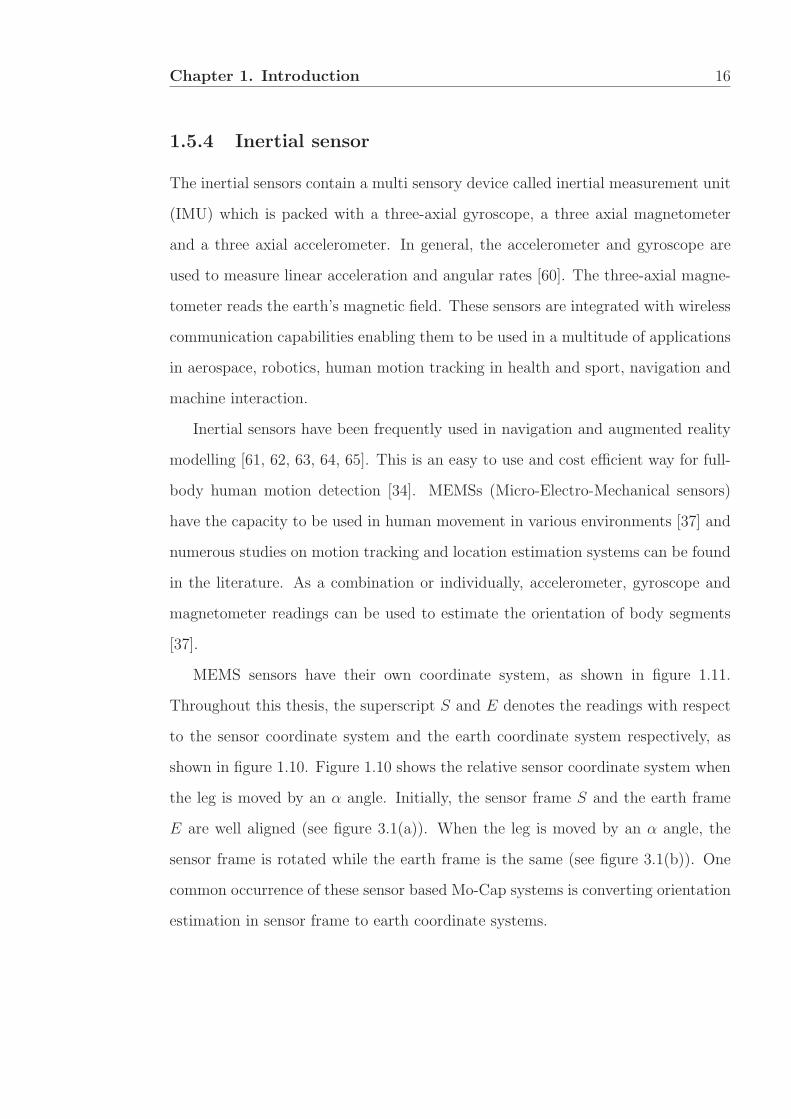
MEMS sensors have their own coordinate system, as shown in figure 1.11.
Throughout this thesis, the superscript S and E denotes the readings with respect
to the sensor coordinate system and the earth coordinate system respectively, as
shown in figure 1.10. Figure 1.10 shows the relative sensor coordinate system when
the leg is moved by an α angle. Initially, the sensor frame S and the earth frame
E are well aligned (see figure 3.1(a)). When the leg is moved by an α angle, the
sensor frame is rotated while the earth frame is the same (see figure 3.1(b)). One
common occurrence of these sensor based Mo-Cap systems is converting orientation
estimation in sensor frame to earth coordinate systems.

Chapter 1. Introduction 17
ASz
ASx
ASy
AEx
AEz
ASy
(a) Before
ASz
α
AAAAAASαα
ASx
AEx
ASy
ASy
AEz
(b) After
Figure 1.10: Earth and sensor co-ordinate systems
There are various commercially available inertial sensors such as Xsens, micro-
strain, VectorNav, Intersense, PNI and Crossbow [66]. MT9 (newly MTx) is a com-
mercially available digital measurement unit and the accuracy is recorded as 0.058
root-mean-square (RMS) angular resolution; � 1.08 static accuracy; and 38 RMS
dynamic accuracy. However, these inertial sensors undergo the error in accuracy
due to drift caused by continuous integration of gyroscope readings. Even though
gyroscope readings suffer from gyroscopic drift, it can be mitigated with the aid of
acceleration readings or magnetometer readings [37]. The current studies in motion
tracking with the aid of inertial sensors and magnetic sensors have shown good
accuracy [37] and most of them were validated with optical fusion technology such
as VICON systems. Further, theoretically, the accelerometer reads gravity, though
practically, it reads resultant acceleration due to interferences in the environment
[67, 68, 69]. On the other hand, since the magnetic north and geographical north
are different and it highly depends on external magnetic fields in the environment,
a proper calibration is required before measurement[39].

Chapter 1. Introduction 18
(a) Xsens sensor- MT9 unit [70] (b) BioKin sensor
Figure 1.11: Rotational angles of inertial sensors
1.5.5 Summary and challenges
The existing rehabilitation and motion tracking systems have been comprehensively
summarised in terms of accuracy, compactness, computation, cost and drawbacks
in table 1.3.
Table 1.3: Comparison of sensor technologies use in rehabilitationTechnology Accuracy Compactness Computation Cost Major Drawbacks
Marker based Visualsystem - VICON sys-tem, Qualisys system
High Low High High Occlusion, High spacerequirement, Operatingskill, limited sensingrange, Not suitable forlong term monitoring
Marker based Visualsystem - Kinect Op-tical System
Median Low High Low Occlusion, limited sens-ing range, Not suitablefor long term monitor-ing
Marker-free VisualSystem
High Low High High Occlusion, limited sens-ing range, Not suitablefor long term monitor-ing
Glove High High Low Median Partial and limited pos-ture, Difficult to wear
Inertial Sensors High High Low Low Drift, Resultant accel-eration
Magnetic Sensors Median High Low Low Interference due to Fer-romagnetic materials
In general, these sensor technologies require professionals to perform calibration
and sampling. These systems do not provide patient-oriented therapy, and hence
cannot be directly used in home-based environments, although the advancements

Chapter 1. Introduction 19
of these technologies are being considered for home use [34].
The second challenge is cost. The affordability of equipment is highly important
for patients, caregivers and medical experts. The cost of Mo-Cap systems is a prime
factor for the uptake of these systems. In certain occasions, the cost is important
than accuracy.
Further, ergonomics based properties such as user friendliness, light weight and
portability of devices are very important. Most people with neurological conditions,
have significant loss of functionality in the attached limbs and therefore need careful
consideration. It has been consistently suggested that the devices need to be quite
user friendly.
Existing rehabilitation systems typically require a large space and specialized
facilities. As a consequence, this prevents people who have less accommodation
space from using these systems to regain their mobility. On the other hand, both
caregivers and patients face difficulties to facilitate patient travel to those clini-
cal laboratories. Further, the clinical environments are not suitable to study their
natural behaviour and sometimes, long term monitoring is required for better un-
derstanding of the underlying condition.
In summary, when one sensor technology is considered for a rehabilitation sys-
tem, number of major issues need to be taken into account: cost, size and weight,
functionality, accuracy, user-friendliness and suitability to dynamic environments.
1.5.6 Motivation to use inertial sensors
In section 1.5.5, the main challenges of the sensor based human motion monitor-
ing and rehabilitation systems were discussed. These challenges entail low cost
healthcare monitoring systems suitable for home use, with remote access for med-
ical professionals and emergency responders. Among these technologies, inertial
sensor based instruments are outperforming than the other methods with respect
to compactness, computation and cost. However, inertial sensor based systems lack

Chapter 1. Introduction 20
accuracy compared to visual tracking systems. Significant attention has been drawn
to inertial sensor based rehabilitation systems due to ease of use and affordability.
Recently, a number of studies have attempted to increase the accuracy by mitigat-
ing the discussed drawbacks such as gyroscope drift, interferences to accelerometer
and magnetic field applying powerful filtering. Inertial sensor based systems have
the potential to be the most leading technology in rehabilitation, if the accuracy
can be enhanced.
1.6 Orientation tracking using inertial sensor mea-
surements
Inertial sensor contains a multi-sensory device called IMU which is used to measure
the moving object’s angular velocity, gravitational forces with the aid of a three-
axial gyroscope and a three-axial accelerometer. Further, these sensor units are
self-contained with a magnetometer, which is able to measure magnetic field of the
earth. The applications of these sensors spread over multiple disciplines such as
aerospace, robotics, navigation and machine interaction. Recently, these sensors
have been developed with wireless capabilities enabling them to be readily used for
determining human activities [71, 72]. On the other hand, they consume very low
power enabling long term monitoring [73] of human activities.
However, these sensors undergo errors in accuracy due to drift caused by contin-
uous integration of gyroscope readings and interferences to accelerometer measure-
ments due to external forces. Further, since the magnetic north and geographical
north are different and it highly depends on external magnetic fields in the envi-
ronment, the magnetometer readings are noisy.
In this study, BioKin sensors as figure 1.12 are being used to conduct exper-
iments. The BioKin project is aimed at introducing a platform to move gesture
analyses, currently restricted to a suitably equipped clinical environment, into an

Chapter 1. Introduction 21
ambulatory system possibly aimed at non-clinical settings, which can provide com-
plementary services to communities with limited access to gait laboratories. The
BioKin system consists of several layers: a low-cost wearable wireless motion cap-
ture sensor, data collection and storage engine, motion analysis algorithm and visu-
alization platform. The first layer is implemented in the BioKin-WMS sensor and
the latter layers are distributed among different components of the BioKin soft-
ware suite: BioKin-PC, BioKin-Cloud and BioKin-Mobi. The BioKin sensor is an
inertial sensor providing 140 Hz sampling frequency.
Figure 1.12: BioKin sensor
Each sensory component of inertial sensors will be further investigated in the
following sections.
1.6.1 Accelerometer
A large number of accelerometer based Mo-Cap systems [74, 75, 76, 77, 78] are
present in the literature. In general, the basic mechanism behind the accelerometer
can be described in terms of a Mass–spring system, which operates under the prin-
ciples of Hookes law (F = kx) and Newtons second law of motion (F = ma)[78].
When a massspring system is submitted to a compression or stretching force due to
movement, the spring will generate a restoring force proportional to the amount of
compression or stretch. Given that the mass, and the stiffness of the spring can be
controlled, the resultant acceleration of the mass element can be determined from
the characteristics of its displacement using two equations F = ma and F = kx.

Chapter 1. Introduction 22
Calibration of accelerometer
There are various types of accelerometers in use and all should undergo a standard
calibration procedure. Usually, there are two calibrations procedures: static cal-
ibration and periodic calibration. Under the static calibration, the accelerometer
readings in a static state will be read. In general, the accelerometer with the global
vertical axis (earth vertical axis) should read gravity which is + or − 9.81ms−2
depending on the direction of vertical axis of the sensor frame. Then a two point
linear calibration is conducted for accelerometer measurements.
Specialised equipment called a shaker is generally used in periodic calibration.
It essentially involves harmonic forcing of the accelerometer to determine the re-
lationship between the known acceleration harmonics and the raw output of the
accelerometer [79]. The accuracy can be enhanced using this method particularly
at a range of amplitudes and frequencies that could be expected under real-world
conditions [79].
Modelling of accelerometer measurements for human activities
The output of an accelerometer worn on the human body originates from several
sources such as 1. Acceleration due to body movements, 2. Gravitational acceler-
ation and 3. External accelerations excluding body movements and accelerations
due to movements of the sensor against other objects or jolting of the sensor on
the body [80]. Hence, the accelerometers read resultant acceleration of all these
acceleration components. Further, accelerometer readings have a constant offset
and a moving bias. The accelerometer readings can be modelled as follows:
at = a+ Ct +Bt +Nt, (1.6.1)
where at, a, Ct, Bt and Nt are the measured accelerometer readings, true arm
rotation, a constant offset or bias, a moving bias and noise at time t respectively
[69].

Chapter 1. Introduction 23
Orientation determination
Initially, the accelerometer needs to be properly calibrated. The noise in acceler-
ation can be removed using low pass filtering up to a certain extent. The filtered
acceleration can be used to estimate the angle of movement(θa) using (1.6.2) [60].
θa = tan−1 ayaz, (1.6.2)
Challenges
The major challenges of using accelerometers for tracking human body movement
can be listed as follows.
1. The output of accelerometer reading is influenced by motion artefacts and
other noise components discussed in section 1.6.1. Hence, the accuracy of
estimation will be reduced.
2. The gravitational acceleration can be only read in the sagittal and the frontal
plane, but not the transverse plane. Hence, human movement in the trans-
verse plane cannot be tracked accurately with accelerometer readings alone.
1.6.2 Magnetometer
Magnetometers are used to measure the strength of earth’s magnetic field and
determine the heading angle to the earth’s magnetic field. The strength of the
earth’s magnetic field is about 0.5 to 0.6 gauss and has a component parallel to the
earth’s surface that always points toward the magnetic north pole. In the northern
hemisphere, this field points down. At the equator, it points horizontally and in the
southern hemisphere, it points up. This angle between the earths magnetic field
and the horizontal plane is defined as an inclination angle. Another angle between
the earth’s magnetic north and geographic north is defined as a declination angle
in the range of ±20◦ depending on the geographic location [81].
Magnetometer readings suffer accuracy errors due to the following reasons:

Chapter 1. Introduction 24
1. The accuracy error due to hard-iron interferences with the magnetic field.
This is prevalent in ferromagnetic materials [81]. Investigations into the ef-
fect of magnetic distortions on an orientation sensor’s performance have shown
that substantial errors may be introduced by sources including electrical ap-
pliances, metal furniture and metal structures within a buildings construction
[66]. The hard iron based error can be corrected by conducting proper cali-
brations.
2. The accuracy error due to soft-iron interferences. This error is generated by
internal devices.
3. Scale factor error due to mismatch of the sensitivity of magnetic sensor sensing
axes. This error can be corrected by normalizing magnetometer readings of
each axis with to earth magnetic field.
4. Declination error due to difference of horizontal plane and earth frame. Addi-
tional heading equipment such as calibration table is required to correct this
error.
Calibration of magnetometer
Magnetometer readings can significantly fluctuate across sensors and locations pri-
marily due to soft-iron interferences in each sensor and the strength of hard iron
interferences in the environment. Hence, calibration should be conducted for sensors
and locations separately.
In the calibration process, the sensor is slowly rotated around each axis while
it is being moved in a lemniscate trajectory between ten to twelve minutes as to
measure the maximum value (MAXxS) and minimum value MINx
S in readings of
each axis. Then, each magnetometer reading is normalized with the earth’s max-
imum magnetic field MAXxE and minimum magnetic field MINx
E using equation
1.6.3. The normalized magnetometer readings (MAGx) are usually free from offset
and scaling error.

Chapter 1. Introduction 25
MAGx =MAXx
E −MINxE
MAXxS −MINx
S
×MAG, (1.6.3)
Eventually, the calibrated sensor readings should be approximately equal to
the actual magnetic readings of the geographical location. In our study, all the
experiments were conducted in Geelong, Victoria, Australia and the magnetometer
readings were as in table 1.4.
Table 1.4: Magnetic fields in Geelong
East Component (nT) North Component (nT) Vertical Component (nT)
4248.95561 21083.6 56226.5
Modelling of magnetometer readings
The calibrated magnetometer readings should be normalised to compensate for tilt.
The normalized magnetometer readings h can be modelled as follows [82].
ht = h+D +Nt, (1.6.4)
where ht, h, D and Nt are normalized magnetometer readings, true earth’s magnetic
field vector, magnetic disturbances and the noise at time t respectively. However, D
can be mitigated by conducting trials at least 60 cm beyond the potential sources
of magnetic disturbances [83], so all the experiments were conducted to mitigate
the magnetic disturbances as in [83].
Orientation determination
The heading angle can be calculated based on (1.6.5) where hx and hy are magne-
tometer readings of x axis and y axis respectively.
Heading = arctan(hy
hx), (1.6.5)

Chapter 1. Introduction 26
Challenges
The major challenges of using magnetometers for tracking human body movements
can be listed as follows.
1. The magnetometer readings are affected by the aforementioned uncertainties
and, hence the estimated movement angles become inaccurate
2. The strength and the direction of the earth’s magnetic field is dependent on
the geographic location and, hence when the heading angle is calculated, more
vertical magnetic directions are susceptible to erroneous deductions
1.6.3 Gyroscope
Gyroscopes are considered for numerous applications [84, 85, 86]. These capture
angular rates in each time stamp. Generally, the angle of rotation is derived by
integrating the angular velocity [84].
Modelling of gyroscope measurements for human activities
When gyroscopes measure the angular rates of each time stamp t, inevitably, it
consists of measurement noise. However, the angular rates are considered to be less
noisy and have a relatively higher accuracy. In order to derive the angle, angular
rates need to be integrated. The integration causes drift which is a major concern.
The measurements of gyroscope can be modelled as (1.6.6).
ωt = ω + Ct +Bt +Nt, (1.6.6)
where ωt ,ω, Ct, Bt and Nt are the measured gyroscope readings, gyroscope readings
for actual arm rotation, a constant offset, a moving bias and a wide band sensor
noise at time t respectively [69].

Chapter 1. Introduction 27
Orientation determination
The gyroscope readings are filtered using a high pass filter. Then, the angular rates
in each t is integrated as (1.6.7) [60].
θω =
∫ t
i=1
f(ωi), (1.6.7)
The gyroscope measurements are always with respect to the sensor frame, hence
it is necessary to convert to the earth frame to estimate the absolute orientation.
For that, the angular rates were integrated and the angle of rotation determined in
each axis with respect to a known reference (initial) position. Rodrigues rotational
formula [87, 39] can be applied to estimate absolute orientation as in (1.6.8) where
vrot is a rotated vector in R3 of the vector �v and K is the unit vector of axis of
rotation.
vrot = �v cos θω + (K × �v) sin θω +K(K.�v)(1− cos θω), (1.6.8)
An alternative approach for this conversion is calculating the quaternion derivative
[88]. Here, the gyroscope readings in the sensor frame ωS at time t is considered as
pure quaternion (1.6.9) and quaternion multiplication (⊗
) is applied for calculating
the derivative as in (1.6.10). Initially, quaternion is considered as[1 0 0 0
]and
then, the quaternion of each time t with respect to the earth frame is calculated as
(1.6.11).
ωSt =
[0 ωS
X ωSY ωS
Z
]t, (1.6.9)
SE qω,t =
1
2SE qt−1
⊗ωSt , (1.6.10)
SEqω,t =
SE qt−1 +
SE qω,tΔt, (1.6.11)
Challenges
Gyroscopic measurement based tracking is associated with the drift which causes
erroneous estimations, therefore mitigating this is essential. It can be mitigated
with a known reference point or direction to a certain extent. However, gyroscope
based tracking is not suitable for longer time frames due to the drift and it should be

Chapter 1. Introduction 28
reset using a known reference point at regular intervals for comparatively accurate
estimations. This is an inconvenient process for long-term monitoring.
1.6.4 Summary
There are numerous advantages and disadvantages with IMU sensors. However, the
fusion of information from these sensory devices can lead to improved accuracies
resulting in reliable systems for multitude of applications. Later sections will inves-
tigate the available approaches for fusion of each sensory modules to acquire better
accuracy compared to individual estimations.
1.7 Wahba’s problem
The orientation estimation of a dynamic object, based on its observation vectors
in local frame and corresponding global frame’s observations, was approached as
a minimizing loss function problem by Grace Wahba in 1965 [89, 90]. Later, this
problem was generally known as Wahba’s Problem in applied mathematics [91].
Thereupon, the solutions to this problem have been improved and these solutions
have been applied to various applications including aerospace, ship navigation, bio-
medical advancements and multi camera calibration in computer vision [92].
Considering Wahba’s problem, some relevant aspects are as follows.
1. A dynamic object with its own coordinate system and moving in a global
coordinate system
2. The orientation of the object with respect to the global coordinate system is
required to determine using the observation vectors
3. There should be static observation vectors which are common to both local
and global coordinate systems
Under Wahba’s problem, the orthogonal matrix for the corresponding rotation is
found between two coordinate systems from a set of weighted observation vectors
Chapter 1. Introduction 29
[93, 90]. First, the reference frame coordinate system and local body coordinate
system were abbreviated as RCS and LCS respectively. The unit vectors measured
in LCS are noted as bi and the corresponding vectors in RCI are noted as ri. Here A
and ai are the rotation matrix between two coordinate systems and the non negative
weight respectively.
L(A) ≡ 1
2
∑i
ai|bi − Ari|2, (1.7.1)
As (1.7.1), the Wahba’s problem is basically a minimization problem to determine
least variance of orientation estimation between RCS (ri, i = 1, 2..n) and LCS
(bi, i = 1, 2..n). Here, i from 1 to n is the number of different observation vectors.
This approach was originally used for spacecraft’s attitudes estimation where the
observation vectors are unit vectors of a star or sun [94, 95, 96]. However, each
solutions of Wahba’s problem is attempted to minimise the loss function (1.7.1)
[90]. Later, this equation is simplified to a convenient form as (1.7.2) [90].
L(A) ≡ λ0 − tr(ABT ), (1.7.2)
where B is∑n
i=1 aibirTi . It is clear that the matrix B is maximised when the least
error of estimation L(A) is minimized. each approach in section 1.7.2 was attempted
to find optimal solution based rotation matrix or quaternion presentation from
(1.7.2).
1.7.1 Applicability of Wahba’s problem for inertial sensorbased orientation estimation
Considering the applicability of Wahba’s problem for tracking human arm move-
ments, Some similarities can be stated satisfying the above three conditions as
follows.
1. The inertial sensor and earth frame are having two different coordinate sys-
tems
2. The earth magnetic field measurements are static measurement, hence it is
common to both frames

Chapter 1. Introduction 30
3. When the object is being moved under constant velocity, the resultant accel-
eration is gravity, hence the acceleration vector is common to both frames
Hence, the solutions for Wahba’s problem are applicable tracking human arm move-
ments [97].
The major benefit of applying these techniques is that the use of gyroscope
readings can be avoided. As we know, Even though gyroscope readings are accu-
rate measurements in sensor frame, the integration causes inaccuracies due to drift
[39]. Further, the solutions of Wahba problem have closed form estimation which
are efficient to compute[97, 98]. In addition, this method needs only two measure-
ments to estimate rotation matrix which gives equivalent result in comparison to
the complementary filter.
1.7.2 Available solutions for Wahba’s problem
TRIAD method
TRIAD method is an initial approach to solve this problem [99], which was intro-
duced by Harold Black. He attempted to find an optimal solution through cosine
matrix of two common observation vectors in LCS and RCS. In this approach, the
observation vectors in LCS (b1 and b2) and the corresponding observation vectors
in RCS (r1 and r2) are normalized and the cross product of each vectors were used
to calculate the optimal rotation matrix (A) as (1.7.3).
A =[
R1
‖R1‖ ,R1×R2
‖R1×R2‖ ,R1
‖R1‖ × R1×R2
‖R1×R2‖
] [r1
‖r1‖ ,r1×r2
‖r1×r2‖ ,r1
‖r1‖ × r1×r2‖r1×r2‖
]T, (1.7.3)
Singular value decomposition method
Subsequently, the SVD method was introduced to solve this problem [100, 101].
The significance of this method is that its outstanding performance even with noisy
observation vectors [90, 101]. Under this method, the U and V orthogonal value is
determined using B matrix using (1.7.2). Then, the determinants detU and detV

Chapter 1. Introduction 31
were obtained. The optimal rotation matrix is estimated using (1.7.4).
L(A) = U
⎡⎢⎢⎣
1 0 0
0 1 0
0 0 (detU)(detV )
⎤⎥⎥⎦V T , (1.7.4)
Davenport’s q method
Davenport introduced this method to determine the attitude of spacecraft [98, 103].
Under the method, trace of ABT in (1.7.2) is written as a homogeneous quadratic
function of quaternion q [90, 98] as (1.7.5).
tr(ABT ) = qTKq (1.7.5)
where K is a symmetric traceless matrix.
K ≡[S − Itr(B) z
zT tr(B)
], (1.7.6)
Here, S is equal to the summation of B and its transpose (B + BT ). z is a 3
by 1 matrix which is equal to the summation of cross product of ri and bi of all
observation vectors. In other words, z =∑n
i=1 aibi × ri (Refer to equations 1.7.1
and equation 1.7.2). Then, the optimal quaternion for the movement is given by
the normalized eigenvector (V ) of K with the largest eigenvalue (D).
Kqopt = λmaxqopt, (1.7.7)
qopt = V < −max(D)), (1.7.8)
QUEST method
The QUaternion ESTimator (QUEST) method was initially introduced in 1979
[90, 104, 105]. Since then, this method is considered as the most applied algorithm
for attitude estimation of spacecraft. Under this method, the fourth order quadratic
method is found λmax in (1.7.7) as follows.
0 = γ[λmax −tr(B)
]− zT
[αI +λmax −tr(B)S +S2
](1.7.9)

Chapter 1. Introduction 32
where
α = λ2max − [tr(B)]2 + tr(adj[S]),
and
γ = α[λmax + tr(B)] + det(S),
λmax can be found for the optimal quaternion using Newton -Raphson iteration
[91]. When the loss function is very small, λ0 will be close to λmax. in which
case, several iterations are required to obtain the optimal(maximum) λ result. The
advantages and disadvantages of the above four methods in general, are listed in
following table.
Table 1.5: Advantages and disadvantages of solutions to the Wahba’s problemTRIAD Method SVD Method Davenport’s q method QUEST Method
Advantages
Simplest Solution Robust algorithm Fast method since theeigenvalues are used
Always gives one op-timal solution becauseof applying Newton-Raphson iterations
Faster than othermethod
Good performancewith noisy data
Robust algorithm Fast algorithm
Robust algorithm High computationalcost
Since optimal quater-nion is estimated, thesingularity problemsare eliminated
Less computation cost
Since optimal quater-nion is estimated, thesingularity problemsare eliminated
Disad
vantages
Singularity problemoccurs since the resultis rotation matrixwith Euler angles
Singularity problemoccurs since the resultis rotation matrixwith Euler angles
Sometimes, unique so-lution will not befound when two ormore eigenvalues areequal to largest eigen-value
Less Robust algorithm
Three primary approaches to human motion analysis using inertial sensors can
be found [106].
1. Systems that use single module of inertial sensors (either accelerometer or
gyroscope) for analysing qualitative information on human motions

Chapter 1. Introduction 33
2. Systems that operate on the basis of a combination of accelerometers and
gyroscopes with additional signal processing algorithms
3. Systems that operate on the basis of both inertial sensor types in combination
with additional sensors (usually magnetometers) and data fusion algorithms
Chapter 2 discusses the second and third type of systems for arm kinematics and
chapter 4 investigates the first type of systems for qualitative analyses of upper
body and lower limbs.
1.8 Contributions
This thesis attempts to introduce novel accurate orientation estimator for human
kinematics while delivering four contributions to inertial sensor based rehabilitation
systems. One contribution is introducing novel orientation estimators for monitor-
ing human activity accurately as in [39, 107]. In addition, a novel calibration mech-
anism for correcting sensor misalignment between sensor frame and earth frame has
investigated as in [108]. With these outcomes, the orientation and angle of move-
ment could be estimated accurately facilitating the capture of human movements.
Limb length is a useful assessment criteria for a common anatomical disease
called limb length discrepancy. This condition makes the disorders in human move-
ments specifically gait cycles with presence of leg length discrepancy (LLD). Hence,
the machine driven mechanism [43] to estimate limb length has been investigated
using only an IMU sensor as the second contribution. Importantly, the above cali-
bration mechanism and limb length estimator are developed by applying curvature
and geometrical relationships of limb trajectories.
As the third contribution, a qualitative analyses of human kinematics were inves-
tigated. Under this, analyses were conducted for evaluating the trunk movements
relevant to Parkinson’s disease based on their kinematic features. Further, the
ambulatory energy expenditure evaluation was conducted to investigate the rela-
tionship between energy consumption for gait exercises such as walking and running

Chapter 1. Introduction 34
as in [109].
Finally, a novel cloud based tele-rehabilitation system based on inertial sensors
was introduced in [110]. This system was then extended to connect other sensory
devices. A multi-level encoding mechanism was introduced in [111] for efficiently
sharing limited resources such as internet bandwidth and mobile phone battery
power while the sensor is transmitting the data to a master server.
1.9 Outline of the thesis
The first chapter is a literature review on human kinematics and available sensor
technologies used for rehabilitation. The principles behind each sensory components
of inertial sensor are comprehensively investigated. In later sections, the histori-
cal attitude determination algorithms are discussed and feasibility for applying in
human motion tracking using inertial sensors is investigated.
The second chapter provides an overview of existing attitude estimators which
are suitable for real time human upper body activity monitoring. Subsequently,
it proposes a novel data fusion algorithm accommodating uncertainty and mea-
surement noise for capturing human motion activities in real-time. Importantly,
the arm kinematics were modelled as a dynamic mathematical model and then,
different data fusion techniques such as extended Kalman filter, robust extended
Kalman filter and introduced novel robust extended Kalman filter with linear mea-
surements are engaged. Further, results are compared with gold standard : VICON
optical system.
In the third chapter, the curvature and geometrical relationships on circular
motions were studied using measurements of inertial sensors. In particular, curva-
ture could be applied in shoulder and hip exercises such as flexion-extension and
abduction-adduction. With the knowledge of these concepts and limb trajectories,
a calibration mechanism for correcting sensor misalignment was introduced. Fur-
ther, a novel approach for estimating limb lengths to assess limb length discrepancy

Chapter 1. Introduction 35
anatomical condition was discussed.
In the fourth chapter, a qualitative analysis on human upper body movements
was investigated. In this chapter, the single type of sensory module (either ac-
celerometer or gyroscope) are used for the analysis of trunk movements. Trunk
movements were compared between healthy subjects and Parkinson patients to
identify physical features of Parkinson’s disease such as rigidity of trunk, slow move-
ments and inflexibility. Further, for the lower body, gait activities were analysed to
examine the relationship between energy expenditure and gait activities.
With the increasing population of aged and people with disabilities, the need
for innovative solutions supporting accurate and personalized medical diagnosis and
treatments at affordable price is highlighted. Furthermore, carefully monitoring of
patient’s activities and physical features can play a significant role in diagnostic
and rehabilitation processes. This highlights the requirement for a multi-sensor
equipped system to cater to all signals to derive valuable information about a pa-
tient. Hence, the tele-rehabilitation system using different sensory technologies is
implemented using cloud web services and mobile phone. The challenges of such
systems are discussed and multi-level encoding mechanism was introduced for effi-
ciently sharing resources.
Finally, the last chapter presents the conclusion of the discussed work and reveals
future directions for further studies based on the thesis.

Chapter 2
Robust Estimation Of ShoulderMovements
2.1 Introduction
Capturing human posture real time with wearable sensors is useful in many practical
applications ranging from rehabilitation, motion capture for movie industry as well
as activity monitoring in sports. IMU sensors are considered widely for this purpose
as its ability to be used in form of wearable sensors. Indeed, the main challenge
is capturing human movements by estimating the relative attitude of IMU sensors
strategically positioned in different parts of the human body.
Capturing highly flexible human poses with 278 joints combining 308 bones is
challenging albeit approximating the movements of inflexible fibrous joints, rela-
tively flexible cartilaginous joints and highly flexible synovial joints into the joints
with more prominent movements. Usually, the human motion is characterized
through carefully analysing spatial reconstruction, trajectory tracking, joint angle
determination and derivative computation [112].
Using inertial/magnetic sensors for capturing human movement has been al-
ready discussed in sections 1.5.4, 1.6.1, 1.6.2 and 1.6.3. IMU sensors have shown
potentiality due to wearable nature, accuracy and three forms of measurements
facilitating the engagement of sensor fusion ideas. The solutions for Wahba’s prob-
lem which discussed in section 1.7 were enhanced with powerful estimators such
36

Chapter 2. Robust Estimation Of Human Shoulder Movements 37
as Kalman filter and extended Kalman filter(EKF) [113]. However, these studies
are conducted under strong assumptions that the rigid body to which the sensor
is attached is stationary or moving at a constant velocity. In other words, these
algorithms are not suitable for highly dynamic tracking applications. Further, De-
viation from ideal behaviour of the sensors due to noise and external interferences
reduces the accuracy of estimations as well.
In this chapter, four major contributions has been discussed for accurate human
motion tracking using inertial/magnetic sensors. Firstly, an unified quaternion
based model for bio-kinematic state estimation is introduced. Secondly, a theoret-
ical justification is conducted for quaternion normalisation required for recursive
estimators. Thirdly, a converted measurement based approach for the formation
of a quasi-linear state estimation problem is introduced. Finally, the robust ex-
tended Kalman filter based approach to estimate the orientation (attitude) of the
human pose subjected to large uncertainties, is introduced. This novel approach is
validated with computer simulation and in a real-time data with a comprehensive
evaluation of existing sensor fusion approaches in a real time estimation domain.
2.2 Data fusion techniques and algorithms
2.2.1 Gradient descent algorithm
The MARG algorithm in [88] represents orientation as a quaternion minimizing
gyroscope drift accommodating novel algorithm. Under this, an analytically derived
and optimized gradient descent algorithm was introduced by Sebastian et al. in 2011
using IMUs, which is shown in figure 2.1.
In this algorithm, the quaternion representation Sω in (2.2.1) is used for esti-
mating the orientation rather than Euler angles.
Sω =[0 ωx ωy ωz
]. (2.2.1)

Chapter 2. Robust Estimation Of Human Shoulder Movements 38
Figure 2.1: Block diagram of MARG algorithm implementation [88]
The quaternion derivative is given by SE q in equation (2.2.2) to convert the mea-
surement in sensor frame to earth frame.
q = 12q ⊗ ω. (2.2.2)
Then, the orientation of the earth frame relative to the sensor frame at time t was
calculated by numerically integrating SE q as in equation (2.2.3).
SEqω,t =
SE qest,t−1 +
SE qω,tΔt (2.2.3)
The optimisation problem in [88] was formulated as equation (2.2.4) and the gradi-
ent descent algorithm was used to identify the orientation of the sensor with respect
to the earth coordinate system.
minSE q∈R4
f(SE q,E d,S s), (2.2.4)
where SE q is the estimated orientation of the sensor, E d is the predefined referenced
earth direction such as gravity or magnetic field and S s is the measured field of the

Chapter 2. Robust Estimation Of Human Shoulder Movements 39
sensor. SE q could be found by MARG algorithm to n iterations with a variable step
size of μ given in equation (2.2.5).
SEqk+1 =
SE qk − μ
Δf(SE qk,E d,S s)
‖Δf(SE qk,E d,S s)‖, k = 0, 1, 2, 3...n (2.2.5)
The error direction of the solution surface was calculated using the objective func-
tion f and its Jacobian, J using equation (2.2.6).
Δf(SE qk,E d,S s) = JT (SE qk,
E d)f(SE qk,E d,S s) (2.2.6)
2.2.2 Complementary filter
The complementary filter was improved by Euston [114] to attitude estimation.
Further, Vasconcelos [115] introduced the time varying complementary filter to
compensate errors due to the drift and Hong [116] proposed a fuzzy logic based
algorithm to correct the error in the gyroscope readings. The traditional comple-
mentary filter is shown in figure 2.2 [60].
Gyro
Low Pass FilterAccelerometer
High Pass Filter
I
A
G
L
H
Figure 2.2: Traditional complementary filter [60]
The rotation angle (θ) can be calculated as in equation (2.2.7) where θω and θa
are angles derived from gyroscope data and acceleration data respectively. K1 and
K2 in equation (2.2.7) are constants and their total value is equal to one.
[θ] = K1× θω +K2× θa (2.2.7)

Chapter 2. Robust Estimation Of Human Shoulder Movements 40
2.2.3 Adaptive complementary filter
The author have introduced an adaptive complementary filter [39] as an advance-
ment of traditional complementary filter. This filter was created by replacing K1
and K2 constants to variables as in equation (2.2.7). The values for K1 and K2 has
been dynamically bound with a linear relationship to minimize the error of angle
estimation.
When the object is stationary or moving in a relatively low acceleration respect
to gravity, the accelerometer reading can be considered only due to the gravity. At
that time with reference to the gravity, the initial orientation can be found using
acceleration readings. However while the object, potentially the human arm, is
being moved, it reads both gravity and acceleration due to forces generate from
muscles. At this point, acceleration based angles are not accurate since it reads
resultant acceleration. Hence the gyroscope angular rates are used to calculate the
angles in real time. At the final stage, acceleration readings are used to correct the
drift.
The initial gyroscope readings and accelerometer readings are (ω =[ωx ωy ωz
])
and (a =[ax ay az
]) respectively. [Aarm] and [k] are the initial coordination of
the arm and the unit vector. Then, as in figure 2.3, the noise free gyroscope readings
(ω) were obtained by applying a high pass filter to ω and the noise free accelerations
(a) were obtained by applying a low pass filter to accelerations.
ω = fh(ω), a = fl(a), (2.2.8)
The rotated angle (θa) was found using equation (1.6.1) [60]. Further, the same
angle( θω) was found using gyroscope data using equation (1.6.7) [60]. The adaptive
complementary filter is given as follows.
[θ] = Vω × θω + Va × θa, (2.2.9)
where Vω and Va are variables which satisfy the following two conditions.

Chapter 2. Robust Estimation Of Human Shoulder Movements 41
High Pass Filter =Higgg (h== reFilteFPass F== (( )))
Low Pass Filter = Lo ww (ww == rreFilteFPass F== (( )))
= (== , ((( , ))
Combine rotationand transition
Complementary Filter
Sensor Frame to Global Frame orr FFra laaabme to Glo
Identify Orientation = ( Iddde= ten= ifyf(( ,y Orier nen, ,n, [atatat ]onoiott , [[ ]])])
Sensor Measurements
Figure 2.3: Adaptive complementary filter
1.
Vω + Va = K (2.2.10)
2.
Vω, Va =
{Vω satisfying Vω ∝ ω
Va satisfying Va ∝ a(2.2.11)
In the first condition, it implies that the summation of Vω and Va is equal to a con-
stant. The second condition implies that the value of Vω is changing proportionally
to change of gyroscope readings and the value of Va is changing proportionally to

Chapter 2. Robust Estimation Of Human Shoulder Movements 42
change of accelerometer readings. The values of Vω in the ith frame were dynami-
cally bound based on following formula.
Vωi =
i∑i=1
[K
ngyro
], (2.2.12)
where ngyro, K and i are the sample size of gyroscope data, a constant and the
index of current frame respectively.
The new orientation of the arm [Aarm] has been found by applying [θ], [k] and
[Aarm] to the Rodrigues rotational formula 1.6.8.
2.2.4 The algorithms for solving Wahba’s solution
The approaches in 1.7 have been investigated with inertial sensor measurements:
accelerometer readings and magnetometer readings as given in figure 2.4. Firstly,
Static Observation Vectors in LCS
Accelerations MagneticOrientations
Low Pass Filtering Calibration
FilteredAccelerations
MagneticOrientations
Optimal Quaternion
Wahba’sSolutions
TRIAD Method
Rotation Matrix
Static Observation Vector in RCS
Earth gravity vectorInitial MagneticOrientation
SVD Method Davenport’s qMethod QUEST Method
Rotation Matrix
Figure 2.4: Orientation estimation using solutions of Wahba’s problem and IMUs
the human arm behaviour was simulated as two scenarios. The first scenario (Ex-
ercise 1) is aimed at simulating shoulder exercises for arm: shoulder to wrist as one

Chapter 2. Robust Estimation Of Human Shoulder Movements 43
limb. Under this, the exercise abduction/adduction was considered as in section
1.3. The measurements of inertial sensor were simulated as it is worn on the wrist
without bending the elbow. Then, the second scenario (Exercise 2) is aimed to at
simulating the arm bending exercise from the elbow, apparently a day-to-day ac-
tivity:lifting a bottle. In this exercise, the elbow was lifted 45 degrees in Y -Z plane
and the wrist was moved by 153 degrees in same plane. Initially, these scenarios
were simulated without measurement noise. Then, the noise was introduced to each
measurements as equations (1.6.1) and (1.6.4) as decreasing Signal-to-Noise Ratio
(SNR) from 60 dB to 5dB. Later, the optimal estimation of movement angle from
each algorithm with noise was compared with the ideal movement without noise as
in figure 2.5.
5 10 15 20 25 30 35 40 45 50 55 600
0.05
0.1
0.15
0.2
0.25
0.3
0.35
0.4
0.45
0.5
0
0.1
0.2
0.3
0.4
0.5
0.6
0.7
0.8
5 10 15 20 25 30 35 40 45 50 55 60 0
0.2
0.4
0.6
0.8
1
1.2
5 10 15 20 25 30 35 40 45 50 55 60
0
0.05
0.1
0.15
0.2
0.25
0.3
0.35
0.4
0.45
0.5
5 10 15 20 25 30 35 40 45 50 55 600
0.2
0.4
0.6
0.8
1
1.2
5 10 15 20 25 30 35 40 45 50 55 60
0.2
0.4
0.6
0.8
1
1.2
5 10 15 20 25 30 35 40 45 50 55 60
(a) (c)(b)
(d) (e) (f)
Root
Mea
n S
quar
e E
rror
in A
ngle
(ra
d)
SNR SNR
SNR SNR SNR
SNR
SVD method / Davenport’s q method TRIAD method QUEST method
Figure 2.5: Simulation Result: (a), (b) and (c) - RMSE of movement angle in X,Y and Z axis for shoulder exercise, (d),(e) and (f) - RMSE of movement angle inrespectively X, Y and Z axis for lifting a bottle exercise
According to the analysis, the angles derived from each approach such as TRIAD
method, Davenport’s q method, SVDmethod and QUESTmethod, were identical in
the absence of noise. However, when the noise was introduced to accelerometer and
magnetometer readings, the estimated angles of each axis were changed. According
to figure 2.5, initially the root mean square error (RMSE) was very small in both
exercises. However, when the Signal-to-noise ratio (SNR) was decreased from 50

Chapter 2. Robust Estimation Of Human Shoulder Movements 44
dB to 20 dB, the RMSE was increased approximately three times than the rate of
RMSE change from 60 dB to 50 dB. The RMSE was significantly changed when
the noise (lesser than 20 dB) was introduced. The same phenomenon could be seen
in sub figures (d), (e) and (f) for the exercise for day-to-day activity. However,
considering sub figures (a) and (b) for exercise 1 and (d) and (f) for exercise 2, the
QUEST algorithm was outperforming compared to other approaches. The QUEST
algorithm has the least RMSE in all noise levels from 5 dB to 60 dB in those figures.
The second least RMSE could be seen in SVD approach and Davenport’s q method.
Further, both SVD method and Davenport’s q method were performing similarly
and hence the trajectories from each approaches were overlapping in every figure.
The least performing algorithm was the TRIAD method. Although, considering
the subfigures (e) and (f), the QUEST algorithm, SVD method and Davenport’s
q method are equally performing until the SNR level is less than 15 dB. TRIAD
method is outperforming other methods which is a valuable aspect in the TRIAD
method.
Real data experiment
The abduction/adduction and flexion/extension exercises as the section 1.3 were
performed under the real time experiments, in order to compare each approaches for
arm exercises. The experiments to validate the algorithm were conducted with ten
healthy subjects (eight males and two females) without any history of orthopaedic or
intramuscular impairments. The actual exercises were conducted having relatively
low speed compared to gravity or constant velocity in order to closely approximate
the simulated environment. Each exercise was conducted wearing the inertial sen-
sors on the left wrist and elbow. The second exercise was designed as lifting a water
bottle from the front of the body to the mouth. The motion was simultaneously
recorded using the VICON optical motion capture system (VICON T40S System)
equipped with eight cameras sampling at 250 Hz. The angles were derived from
output of the VICON system. During the analysis, VICON data were re-sampled

Chapter 2. Robust Estimation Of Human Shoulder Movements 45
(a) (b)
(c) (d)
Mov
emen
t an
gle
(in ra
d)M
ovem
ent
angl
e (in
rad)
RM
SE in
mov
emen
t an
gle
(in ra
d)R
MSE
in m
ovem
ent
angl
e (in
rad)
sample time
sample time
sample time
sample time
SVD method / Davenport’s q method TRIAD methodQUEST method VICON Optical System data
0 200 400 600 800 1000 12006
4
2
8
6
4
2
0
2
0 200 400 600 800 1000 12000
1
2
3
4
5
6
7
0 50 100 150 200 250 300 350 400 4500
2
4
6
8
1
2
4
6
0 50 100 150 200 250 300 350 400 4500
1
2
Figure 2.6: Experiment result: (a) - movement angle for abduction exercise, (b) -root mean square error in movement angle for abduction exercise, (c) - movementangle for lifting water bottle exercise and (d) - root mean square error in movementangle for lifting a bottle exercise
at 140Hz for comparison purposes. The movements of the wrist were analysed.
Table 2.1: Root mean square error for flexion-extension exercise
TRIAD method Davenport’s q method SVD method QUEST method
Subject 1 0.287 0.2582 0.2582 0.1267Subject 2 0.0633 0.0713 0.0713 0.0704Subject 3 0.1752 0.0537 0.0537 0.0554Subject 4 0.0717 0.0638 0.0638 0.0691Subject 5 0.0544 0.1138 0.1138 0.0554Subject 6 0.0624 0.0686 0.0686 0.0724Subject 7 0.1205 0.0705 0.0705 0.0403Subject 8 0.0453 0.0204 0.0204 0.0281Subject 9 0.0864 0.0781 0.0781 0.0699Subject 10 0.0813 0.0801 0.0801 0.0634
Overall 0.10475 0.08785 0.08785 0.06511
The root mean square errors of the movement angle for each exercise were anal-
ysed and listed in table 2.1 and 2.2. According to table 2.1 for flexion/extension,
table 2.2 for abduction/adduction and 2.3 for lifting water bottle, in general, the

Chapter 2. Robust Estimation Of Human Shoulder Movements 46
QUEST algorithm has the least error compared to other methods. The aver-
age RMSE values for all subjects for exercise 1 :abduction/adduction and flex-
ion/extension were respectively 0.0651 radians and 0.0608 radians. Further, the
average RMSE for lifting exercise is 0.0987 radians for QUEST algorithm. The
Davenport’s q method and SVD method performed equally in each of the exer-
cises and they have the second least error. The highest error could be observed in
TRIAD method for three exercises. This result is shown in figure 2.7. Importantly,
the same phenomenon could be observed in simulation for the same exercise.
1 2 3 4 5 6 7 8 9 100
0.05
0.1
0.15
0.2
0.25
Subjects
Roo
t Mea
n Sq
uare
d Er
ror (
in ra
dian
s)
1 2 3 4 5 6 7 8 9 100
0.05
0.1
Subjects
Roo
t Mea
n Sq
uare
d Er
ror (
in ra
dian
s)
0.15
(A) Flexion -Extension Exercise (B) Abduction - Adduction Exercise
TRIAD Method Davenport q Method SVD Method QUEST Method
0.3
1 2 3 40
0.05
0.1
0.15
0.2
0.25
0.3
Subjects
Roo
t Mea
n Sq
uare
d Er
ror (
in ra
dian
s)
(C) Lifting a bottle Exercise
0.35
Figure 2.7: Experiment result: (a), (b) and (c) - root mean squared error of move-ment angle for extension/flexion exercise, abduction/adduction exercise and liftinga bottle exercise respectively
Table 2.2: Root mean square error for abduction-adduction exercise
TRIAD method Davenport’s q method SVD method QUEST method
Subject 1 0.0802 0.0841 0.0841 0.0481Subject 2 0.0438 0.0574 0.0574 0.0579Subject 3 0.1008 0.0785 0.0785 0.0793Subject 4 0.1299 0.049 0.049 0.0473Subject 5 0.1424 0.1215 0.1215 0.125Subject 6 0.0703 0.0769 0.0769 0.0674Subject 7 0.0152 0.043 0.043 0.0491Subject 8 0.0283 0.04 0.04 0.0434Subject 9 0.0274 0.0372 0.0372 0.0464Subject 10 0.1116 0.0512 0.0512 0.0438
Overall 0.07499 0.06388 0.06388 0.06077
On the other hand, according to table 2.3 for lifting a bottle exercise, the same
trend could be seen for exercise 1. However, under exercise 1, it rotates through

Chapter 2. Robust Estimation Of Human Shoulder Movements 47
Table 2.3: Root mean square error for lifting a bottle exercise
TRIAD method Davenport’s q method SVD method QUEST method
Subject 1 0.1593 0.1178 0.1178 0.0681Subject 2 0.1441 0.0817 0.0817 0.0745Subject 3 0.3408 0.2067 0.2067 0.2085Subject 4 0.0611 0.2174 0.2174 0.0438Overall 0.1763 0.1559 0.1559 0.0987
only one joint which is the shoulder joint. The lifting exercise is considered as a
comparatively complex one, because the arm rotates through two joints such as the
shoulder joint and the elbow joint. Further, when the lower arm is being lifted from
the elbow, this exercise is no longer a planar movement like abduction-adduction
because the lower limb is slightly twisting towards the body. The QUEST algo-
rithm was superior to the other methods even with this kinematic complexity as in
the result in table 2.3. This demonstrates the higher robustness of the algorithm
for complex day-to-day exercises. The external accelerations such as force from
arm muscles, will be observed when conducting complicated exercise such as the
lifting exercise. The second least RMSE was observed in Davenport’s q method
and SVD which is 0.1559 radians. Likewise, the highest error was shown in TRIAD
method. However, the accuracy is slightly reduced in the lifting exercise than the
first exercises. Importantly, the impact of external accelerations may affect the es-
timation. However, the QUEST method performed better in real-time environment
in line with our previous observations in a simulated environment. According to
the computer simulation and real time experiments, QUEST algorithm outperforms
than the other algorithms considered for the simple arm exercises such as flexion-
extension and abduction-adduction. However, the accuracy for complicated arm
exercises such as internal/external rotation for day-to-day activities is expected to
be reduced compared to the simple exercises. This implies that the QUEST method
should be improved for complicated exercises to enhance accuracy by integrating
powerful data fusion and optimization mechanisms.

Chapter 2. Robust Estimation Of Human Shoulder Movements 48
2.2.5 Kalman filter
Kalman filter was initially developed by Rudolf Emil Kalman to solve the problem
of estimating the trajectory for the Apollo program in the NASA Ames Research
centre [117, 118]. It is commonly used as a powerful method for sensor data fusion.
Further, it can also be used to estimate the system state at a given time of a
known dynamic model specified control inputs. Kalman filter is commonly used as
an estimation algorithm, because it has proven better accuracy compared to other
non-iterative methods. However, It has several deficiencies such as linear regression
iterations in the Kalman process and demand sampling rates which can exceed the
subject bandwidth [88].
In general, Kalman filter is defined as linear, discrete time, finite dimensional
time-varying system estimating the system state by minimizing mean square error
[119]. It runs through iterative process of filtering and predicting. Each of these
iterations are derived and interpreted as Gaussian probability density functions. A
typical application of Kalman filter is illustrated as in figure 2.8 [119].
Figure 2.8: The Kalman filter [119]

Chapter 2. Robust Estimation Of Human Shoulder Movements 49
2.2.6 Extended Kalman filter
The conditional probability density functions that provide the minimum mean
square estimation are no longer Gaussian [119], when the state dynamics or ob-
servation dynamics are non-linear. For such circumstances, the extended Kalman
filter: the non-linear version of Kalman filter, is applied. It linearizes about an
estimation of current mean and covariance.
Indeed, the state transition model xk and observation model zk are non-linear
or a differentiable function as equations (2.2.13) and (2.2.14) [119].
xk = f(xk−1, uk−1, wk−1) (2.2.13)
zk = f(xk, vk) (2.2.14)
There are four main steps in the formulation of EKF[120]. x(k|k), u(k), P (k|k) areknown inputs and the new measurement is z(k + 1).
1. State Prediction x(k + 1|k) = F (k)x(k|k) +G(k)u(k)
2. Measurement Prediction z(k + 1|k) = H(k)x(k + 1|k)
3. Measurement Residual v(k + 1) = z(k + 1)− z(k + 1|k)
4. Updated State Estimate: x(k + 1|k + 1) = x(k + 1|k) +W (k + 1)v(k + 1)
W (k + 1) is known as Kalman gain.
Quaternion-based extended Kalman filter
Numerous studies were conducted on 2D and 3D human motion tracking applying
Kalman filter and extended Kalman filter (EKF) such as Azuma and Bizop in 1994
[121, 122], Foxlin et al. in 1996 - 1998 [123, 124], E.R. Bachmann in 2000-2011
[113, 125, 126] and Sebatini et al. in 1995-2013 [127, 128, 129, 130]. The outcomes
of those studies applying EKF for the measurement vectors from inertial/magnetic
sensors has shown better accuracy improvement in obtaining the orientation. Xi-
aoping Yun et al. has introduced quaternion based EKF and the quaternion was

Chapter 2. Robust Estimation Of Human Shoulder Movements 50
Figure 2.9: Extended Kalman filter [113]
calculated applying QUEST method (refer 1.7.2) using accelerometer measurements
and magnetometer measurements.
The use of quaternion rather than Euler angles has following advantages [113].
1. Quaternion based estimation avoids trigonometric functions, hence it compu-
tationally efficient and easier to implement
2. It avoids the singularities
3. Simple as the rotational complicities can be ignored.
The quaternion derivative SE q is the rate of change of the earth frame relative
to the sensor frame and it was obtained using gyroscope readings as in equation
(2.2.2). In [113], two approaches were presented for calculating the quaternion as
given in figures 2.10 and 2.11.
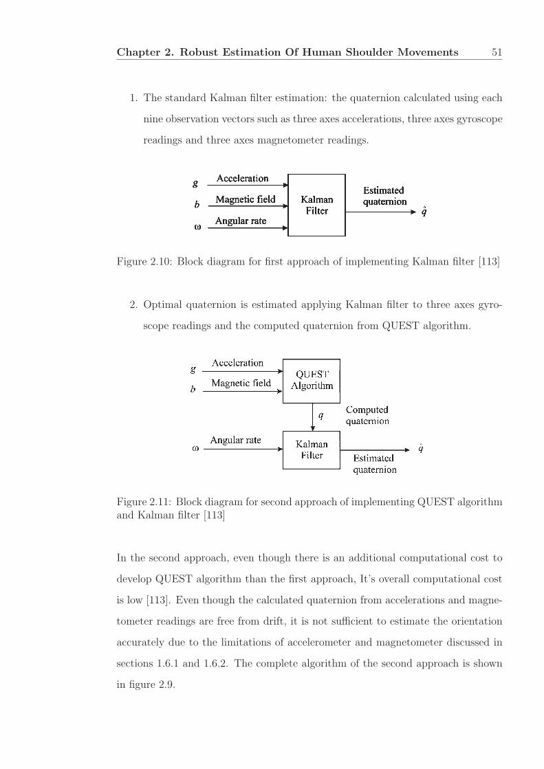
Chapter 2. Robust Estimation Of Human Shoulder Movements 51
1. The standard Kalman filter estimation: the quaternion calculated using each
nine observation vectors such as three axes accelerations, three axes gyroscope
readings and three axes magnetometer readings.
Figure 2.10: Block diagram for first approach of implementing Kalman filter [113]
2. Optimal quaternion is estimated applying Kalman filter to three axes gyro-
scope readings and the computed quaternion from QUEST algorithm.
Figure 2.11: Block diagram for second approach of implementing QUEST algorithmand Kalman filter [113]
In the second approach, even though there is an additional computational cost to
develop QUEST algorithm than the first approach, It’s overall computational cost
is low [113]. Even though the calculated quaternion from accelerations and magne-
tometer readings are free from drift, it is not sufficient to estimate the orientation
accurately due to the limitations of accelerometer and magnetometer discussed in
sections 1.6.1 and 1.6.2. The complete algorithm of the second approach is shown
in figure 2.9.

Chapter 2. Robust Estimation Of Human Shoulder Movements 52
After obtaining the appropriate parameters to initialize EKF, it was simulated
using the observation vectors of MARG sensors. Finally, the real-time quaternion
was produced by EKF, which was visualized using an avatar.
2.2.7 Robust extended Kalman filter
The first appearence of robust Kalman filtering was in 1992 as a potential method
to address the lack of robustness issue which is a significant shortcoming in the state
space control theory [131]. Ian R. Peterson and Andrey V. Savkin has introduced
this improved version of Kalman filter by addressing the issues of robustness against
a large parameter uncertainty in the linear process model. Furthermore, the robust
Kalman filter is available to both linear systems and non-linear systems. The robust
extended Kalman filter (REKF) is the nonlinear form of robust Kalman filter. These
two versions were applied in node localization of mobile robots [132, 133]and missile
guidance [134, 135, 136]. However, these methods are not widely used in human
motion tracking which is our area of interest.
The REKF for a nonlinear uncertain system can be formulated as follows
x = A(x, u) + B2w (2.2.15)
z(t) = K(x, u) (2.2.16)
y = C(x) + v (2.2.17)
where (2.2.15) is the state equation, z(t) in (2.2.16) are uncertainty outputs and
(2.2.17) is the measurement equation. The approximate solutions for the above
problem can be written as equations 2.2.18 and 2.2.19 [133].
˙x(t) = A(x(t), u0) +X−1[ΔxC(x(t))TR(y0 − x(t)) (2.2.18)
+ΔxK(x(t), u0)TK(x(t), u0)], x(t) = x0
X = ΔxA(x(t), u0)TX +XΔxA(x(t), u
0) +XB2Q−1BT
2 X (2.2.19)
−ΔxC(xT )RΔxC(x) + ΔxK(x(t), u0)TΔxK(x(t), u0) = 0

Chapter 2. Robust Estimation Of Human Shoulder Movements 53
2.2.8 Comparison and summary
The data fusion and filtering mechanisms are categorised into two categories as
model based state estimators and ordinary data fusion techniques. The complemen-
tary filter and adaptive complementary filter are listed under the ordinary filtering
techniques. The Kalman filter, extended Kalman filter, robust Kalman filter and
robust extended Kalman filters are listed under the model based state estimators.
Comparison of filtering mechanisms
Firstly, estimation accuracy of the ordinary data fusion techniques such as high pass
filter, low pass filter, complementary filter and adaptive complementary filter have
been evaluated compared to the VICON system. For that, the author conducted an
action of lifting a bottle discussed in section 2.2.4 as an experiment. Figures 2.12(a)
and 2.12(b) show the exercise procedure and the experiment setup respectively.
(a) The exercise procedure (b) Experimental setup
Figure 2.12: Lifting a bottle: VICON markers and BioKin sensors were attachedto the arm (Left arm).
The elbow joint angle variation of each subject was calculated using the following
methods:

Chapter 2. Robust Estimation Of Human Shoulder Movements 54
1. High-pass filtered angular rate integration (θω) (To ensure experimental sim-
plicity manually adjusted the initial orientation to match VICON data)
2. Direct orientation estimation from low-pass filtered acceleration measure-
ments (θa)
3. Sensor fusion using the adaptive complementary filter using (2.2.9)
4. Sensor fusion using traditional complementary filter using (2.2.7)
5. Using VICON motion capture data.
For the traditional complementary filter, the constant K1 for gyroscope as in
equation (2.2.7), was 0.98 and the constant K2 was 0.02. The Root Mean Square
Error (RMSE) was used to estimate the error between trajectories (figure 2.13 shows
for subject 1) in which derived from the sensor measurements and the VICON
optical motion capture system as in table 2.4.
0 50 00 2 0−180
−160
−140
−120
−100
−80
−60
−40
−20
0
Time
Ang
le (d
egre
es)
High Pass Filter GyroscopeLow Pass FilterAccelerations
The Ground Truth
Figure 2.13: Elbow angles were calculated with different filtering and sensor fusiontechniques compared to VICON optical motion capture system for subject 1

Chapter 2. Robust Estimation Of Human Shoulder Movements 55
Table 2.4: The root mean square error comparison of each methods
Method Subject 1 Subject 2 Subject 3 Subject 4
High Pass Filter - Gyroscope 8.918◦ 11.735◦ 6.301◦ 13.779◦
Low Pass Filter - Accelerations 16.484◦ 20.173◦ 31.032◦ 5.522◦
Traditional ComplementaryFilter 8.974◦ 11.853◦ 6.785◦ 13.596◦
Adaptive ComplementaryFilter 7.083◦ 11.270◦ 7.929◦ 8.803◦
As figure 2.13, the plot from the high pass filter on the gyroscope measurements
and the plot from traditional complementary filter were overlapped on each other.
Further, the calculated angles were highly dependent on the accelerations of the
subject’s motion. Subject 4 has shown a better accuracy in the method of low pass
filter compared to others because the particular motion conducted in a very low ac-
celeration. However, this effect has been limited in other three subjects. From table
2.4, the least RMSE of the elbow joint angle and least deviation between minimum
error and maximum error (4.187 degrees) were observed in the adaptive complemen-
tary filter. The deviation in error for other methods: gyroscope based, accelerations
Table 2.5: Advantages and disadvantages of data fusion algorithmsOrdinary filtering techniques Model based state estimators
Complementary filter Adaptive complemen-tary filter
Kalman filter EKF REKF
Advantages Easy to implement
and less computations[39, 137]
Easy to implementand less computations[39, 137]
Noise parameters ofthe measurementsare considered [137]
Noise parameters ofthe measurements areconsidered [137]
Not only noise param-eters but uncertaintyof measurements isalso considered, hencevery robust algorithm
Lower accuracy Average accuracy butbetter than comple-mentary filter [39]
Higher accuracy Higher accuracy Higher accuracy
Simple equations [39,137]
Simple equations [39] Suitable for non-linear systems whichare very common inreal life
Suitable for non-linear systems whichare very common inreal life
Disad
vantages Accuracy is low with
large noise and uncer-tainty
Accuracy is low withlarge noise and uncer-tainty
Complex equationsand calculations
Complex equationsand calculations
Complex equationsand calculations
Not consider any sta-tistical description forthe noise corruptingthe signals [137]
Not consider any sta-tistical description forthe noise corruptingthe signals [137]
Not account-ing uncertaintyparameters of mea-surements, henceless robust [132]
Not accounting uncer-tainty parameters ofmeasurements, henceless robust [132]
Not robust Not robust

Chapter 2. Robust Estimation Of Human Shoulder Movements 56
based and traditional filter are 7.478, 25.5099, 6.811 degrees respectively.
With these experimental results and previous studies in open literature, the
advantages and disadvantages of these data fusion mechanisms are listed in table
2.5.
Model based state estimator implementation relevant to human arm kinematics
is discussed in the next sections of this chapter.
2.3 Dynamic model
General superior performance of dynamic model based estimations inevitably pro-
vides a natural choice for human pose estimation. Identification of a proper dynamic
model facilitating dynamic parameter estimation of rotating and translating frame
is crucial. Indeed the model can be further improved by incorporating full body
human bio-kinematic modelling and here, the author try to keep the overall model
simple to highlight the key contributions of this work. Further, the quaternion
based approach is preferred as it eliminates the issues stated in section 2.2.6. The
nomenclature is included in table 1, Appendix I.
Denoting the orientation quaternion in the earth coordinate frame as q, angular
velocity ω, (2.3.1) is stated as [138],
q = 12q ⊗ ω , (2.3.1)
where, ⊗ denotes the quaternion multiplication with ω = [0 ω1 ω2 ω3]� used as a
pure quaternion. Here vector x is [x1 x2 x3 x4 x5 x6 x7 x8 x9 x10].
Defining the state vector as,
x = [x1 x2 x3 x4 x5 x6 x7 x8 x9 x10]� , (2.3.2)
where,
[x1 x2 x3] = [ω1 ω2 ω3] = ω,
[x4 x5 x6 x7] = [q1 q2 q3 q4] = q,
[x8 x9 x10]� = δ.

Chapter 2. Robust Estimation Of Human Shoulder Movements 57
ω, q and δ are angular rates, quaternions and gyro drift respectively, the dynamic
model can be stated as,
x = A(x) +Ww,where
A(x) =
⎡⎢⎢⎢⎢⎢⎢⎢⎢⎢⎢⎢⎢⎢⎢⎢⎢⎢⎢⎢⎢⎢⎢⎢⎢⎣
− 1τxx1
− 1τyx2
− 1τzx3
x3x5−x2x6+x1x7
2√
x24+x2
5+x26+x2
7
−x3x4+x1x6+x2x7
2√
x24+x2
5+x26+x2
7
x2x4−x1x5+x3x7
2√
x24+x2
5+x26+x2
7
−x1x4−x2x5−x3x6
2√
x24+x2
5+x26+x2
7
− 1dxx8
− 1dyx9
− 1dzx10
⎤⎥⎥⎥⎥⎥⎥⎥⎥⎥⎥⎥⎥⎥⎥⎥⎥⎥⎥⎥⎥⎥⎥⎥⎥⎦
∈ R10×1
W =
⎡⎢⎢⎢⎢⎢⎢⎢⎢⎣
I3 O3×3
O4×3 O3×3
O3×3 I3
⎤⎥⎥⎥⎥⎥⎥⎥⎥⎦∈ R10×6
w = [Tx, Ty, Tz, B1, B2, B3]� (2.3.3)
Here, Tx, Ty, Tz indicate the torque due to uncertain human movements andB1, B2, B3
indicate the uncertainty in the bias responsible for the Gyroscopic drift. Im and
Om×n denotes identity and zero matrix of indicted sizes. The measurement model
can be stated as follows,
y = C(x) + v, (2.3.4)
where y = [y1 · · · y13]� =[ω1 ω2 ω3 a1 a2 a3 h1 h2 h3 x4 x5 x6 x7
]�, is the IMU
measurement vector with angular rate from gyroscopes, acceleration from accelerom-
eters and orientation of the earth magnetic field from magnetometers. Here, v =
[v1 v2 v3 0 0 0 0 0 0]� is the measurement noise. Further, the time constant for

Chapter 2. Robust Estimation Of Human Shoulder Movements 58
the motion and variance of continuous white noise is denoted respectively by τ =
[τx τy τz]� and d = [dx dy dz]
� [139].
C(x) =
⎡⎢⎢⎢⎢⎢⎢⎢⎢⎢⎢⎢⎢⎢⎢⎢⎢⎢⎢⎢⎢⎢⎢⎢⎢⎢⎢⎢⎢⎢⎢⎣
x1 + x8
x2 + x9
x3 + x10
−2‖g‖ (x5x7 − x4x6)
−2‖g‖ (x4x5 + x6x7)
−‖g‖ (x24 − x25 − x26 + x27)
2he2 (x5x6 + x4x7) + 2he3 (x5x7 − x4x6)
he2 (x24 − x25 + x26 − x27) + 2he3 (x6x7 + x4x5)
2he2 (x6x7 − x4x5) + he3 (x24 − x25 − x26 + x27)
x4
x5
x6
x7
⎤⎥⎥⎥⎥⎥⎥⎥⎥⎥⎥⎥⎥⎥⎥⎥⎥⎥⎥⎥⎥⎥⎥⎥⎥⎥⎥⎥⎥⎥⎥⎦
(2.3.5)
Let the measurement in the earth frame have g = [0 0 − ‖g‖]� and he =[0 he2 h
e3
]�acceleration and magnetometer readings respectively.
Remark 1. Without the loss of generality, the X axis of the stationary globalco-ordinate frame in a perpendicular direction to the magnetic direction has beenaligned to simplify the resulting expressions.
Considering (2.3.4), an unique solution is given by,
xm =
√Km+
√K2
m+4L2m
2m ∈ {4, 6}
xn =
√−Kn+
√K2
n+4L2n
2n ∈ {5, 7}
where
K4 = K5 =p2 + q3
2, L4 = L5 =
q2−p32,
K6 = K7 =p2 − q3
2, L6 = L7 =
q2+p32

Chapter 2. Robust Estimation Of Human Shoulder Movements 59
with
p2 =h2‖g‖+a2he
3
he2‖g‖
, p3 =h3‖g‖+ a3h
e3
2he2‖g‖q2 = −a2
2‖g‖ , q3 =−a3‖g‖ . (2.3.6)
Considering the measurement uncertainty, let the measurement model for the con-
verted measurements with respect to magnetometer and accelerometer measure-
ments be:
ai = ai + vai , hej = hej + vej , hj = hj + vhj (2.3.7)
∀i ∈ {1, 2, 3} and j ∈ {2, 3}.
where, ai, hej and hj indicates the accelerometer readings subjected to measure-
ment noise, magnetometer measurement in the earth frame and the mobile frame
respectively. The error bounds are described in the following form:
Assumption 1. The following holds
1 For given constants α and β, let 0 ≤ vai ≤ βai, 0 ≤ vej ≤ αhej and 0 ≤ vhj ≤αhj ∀i ∈ {1, 2, 3} and j ∈ {2, 3}.
In the case of converted measurements, let’s define the following:
μ = (1+α)(1+β)(1−α)(1−β)
, σ = (1−α)(1−β)(1+α)(1+β)
(2.3.8)
λ =√
μ+σ2, φ =
√μ−σ2, (2.3.9)
Now the converted measurement can be stated as,
xi = λxi + ni (2.3.10)
and
‖ni(t)‖ ≤ ‖φxi‖ ∀i ∈ [4, 5, 6, 7] (2.3.11)
Denoting
C =
⎡⎣ I3 O3×4 I3
O4×3 λI4 O4×3
⎤⎦ and
K =
⎡⎣ I3 O3×4 I3
O4×3 φI4 O4×3
⎤⎦
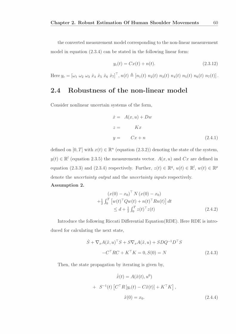
Chapter 2. Robust Estimation Of Human Shoulder Movements 60
the converted measurement model corresponding to the non-linear measurement
model in equation (2.3.4) can be stated in the following linear form:
yc(t) = Cx(t) + n(t). (2.3.12)
Here yc = [ω1 ω2 ω3 x4 x5 x6 x7]�, n(t) � [n1(t) n2(t) n3(t) n4(t) n5(t) n6(t) n7(t)] .
2.4 Robustness of the non-linear model
Consider nonlinear uncertain systems of the form,
x = A(x, u) +Dw
z = Kx
y = Cx+ n (2.4.1)
defined on [0, T ] with x(t) ∈ Rn (equation (2.3.2)) denoting the state of the system,
y(t) ∈ Rl (equation 2.3.5) the measurements vector. A(x, u) and Cx are defined in
equation (2.3.3) and (2.3.4) respectively. Further, z(t) ∈ Rq, u(t) ∈ R
l, w(t) ∈ Rp
denote the uncertainty output and the uncertainty inputs respectively.
Assumption 2.
(x(0)− x0)�N (x(0)− x0)
+12
∫ T
0
[w(t)�Qw(t) + n(t)�Rn(t)
]dt
≤ d+ 12
∫ T
0z(t)�z(t) (2.4.2)
Introduce the following Riccati Differential Equation(RDE). Here RDE is intro-
duced for calculating the next state,
S +∇xA(x, u)�S + S∇xA(x, u) + SDQ−1D�S
−C�RC +K�K = 0, S(0) = N (2.4.3)
Then, the state propagation by iterating is given by,
˙x(t) = A(x(t), u0)
+ S−1(t)[C�R [yc(t)− Cx(t)] +K�K
],
x(0) = x0. (2.4.4)

Chapter 2. Robust Estimation Of Human Shoulder Movements 61
The earth frame is oriented with the following assumptions.
1. Accelerations apart from gravity is negligible
2. Earth frame is such that the direction of the magnetic field is perpendicular
to the X axis.
Remark 2. Notice here that the there is a significant component of the earth mag-netic field in the Z direction in Australia and this cannot be neglected unlike in thecase for locations close to the equator.
Robustness of the estimation
The approximate solution for the set of estimated states for the robust set valued
state estimation is :
χs ={x ∈ Rn : 1
2(x− x(s))�X(s) (x− x(s)) ≤ d− φ(s)
}(2.4.5)
where
φ(t) �∫ t
0
[12(y − Cx)�R (y − Cx)− x�K�Kx
]dτ
Therefore, the centroid of the ellipsoidal set is taken as the estimated state. Let
Φ and Θ denote the diagonalising and the resulting diagonal matrix respectively
while ai and aj denote the spectral densities of 1√d−φ(s)
Θ and√d− φ(s) Θ−1 re-
spectively. Taking, δ+ = [0 · · · ai · · · ]� ∈ Rn and δ− = [0 · · · aj · · · ]� ∈ Rn and
noticing Φ�X(s)Φ = Θ, x+ = x(s) + Φδ+ and x− = x(s) + Φδ− indicate the major
axis and the minor axis of the set values state estimation. This provides a measure
of the estimation bounds.

Chapter 2. Robust Estimation Of Human Shoulder Movements 62
2.5 Robust optimisation based approach for ori-
entation estimation
The x4, x5, x6 and x7 of the state vector denotes the orientation quaternion. With
R+ denoting the set of non-negative real numbers, define,
F (x) = (x4 − P )2 + (x5 −Q)2 + (x6 −R)2 + (x7 − S)2,
G(x) = −2Px4 − 2Qx5 − 2Rx6 − 2Sx7,
x = [x4 x5 x6 x7]T , A1 = [1 0 0 0]T ,
A2 = [0 1 0 0]T , A3 = [0 0 1 0]T , A4 = [0 0 0 1]T ,
Γ =√P 2 +Q2 +R2 + S2, p1 =
1Γ[P Q R S]� ,
p2 =−1Γ[P Q R S]�
Ω = {x ∈ R4+ : x24 + x25 + x26 + x27 = 1},
Λ =
⎧⎪⎪⎨⎪⎪⎩x ∈ R
4+ :
x24 + x25 + x26 + x27 ≤ 1
and
x4 + x5 + x6 + x7 ≥ 1
⎫⎪⎪⎬⎪⎪⎭ ,
∂Λis a boundary ofΛ.
h4 = {x ∈ R4+| x4 = 0}, h5 = {x ∈ R
5+| x5 = 0},
h6 = {x ∈ R4+| x6 = 0}, h7 = {x ∈ R
5+| x7 = 0},
h8 = {x ∈ R4+| x4 + x5 + x6 + x7 = 1},
Λ4 = (∂Λ\Ω)⋂h4,Λ5 = (∂Λ\Ω)⋂h5,Λ6 = (∂Λ\Ω)⋂h6,
Λ7 = (∂Λ\Ω)⋂h7,Λ8 = (∂Λ\Ω)⋂h8Now, the following lemma can be stated as,
Lemma 1. The solution to the following problem of,
minF (x) subjected to x ∈ Ω
can be stated as follows:
1 If P = Q = R = 0 then[12
12
12
12
]�is the optimal solution.
2 if P ≥ 0, Q ≥ 0, R ≥ 0, S ≥ 0 then optimal value of (OP )1 is
min{F (A1), F (A2), F (A3), F (A4), F (p1)}
3 if P ≤ 0, Q ≤ 0, R ≤ 0, S ≤ 0 then optimal value of (OP )1 is
min{F (A1), F (A2), F (A3), F (A4), F (p2)}

Chapter 2. Robust Estimation Of Human Shoulder Movements 63
4 Else the optimal value of (OP )1 is
min{F (A1), F (A2), F (A3), F (A4)}.
Proof. From lemma 3 and 4 in Appendix I, if x∗ ∈ Ω is an optimal point of problem(OP )3 then it also is an optimal point of problem (OP )1. Therefore, to solveproblem (OP )3, an optimal point x∗ ∈ Ω need to be found for problem (OP )3.
For γ ∈ R, the author denote the γ-level set for linear functional G(x) as follows.
Gγ = {x ∈ R4| G(x) = γ}.
Clearly, Gγ, γ ∈ R are parallel hyperplanes. Therefore, if Gγ0 is a supportinghyperplane of the convex set Λ at x0 ∈ ∂Λ then x0 is an optimal point and G(x0) =γ0 is the optimal value of problem (OP )3. Similar to the proof of lemma 3, if x0
belongs to one of five sets Λi, i = 4, 5, · · · , 8 then one of four points A1, A2, A3,A4 is an optimal point of problem (OP )3. On the other hand, Gγ0 is a supportinghyperplane of the convex set Λ at x0 = [x04 x
05 x
06 x
07]
T ∈ Ω if
x04P
=x05Q
=x06R
=x07R
(2.5.1)
(for case P = 0, Q = 0, R = 0.) In this case, (2.5.1) implies that
(x04)2
P 2=
(x05)2
Q2=
(x06)2
R2=
(x07)2
R2
=(x04)
2 + (x05)2 + (x06)
2 + (x07)2
P 2 +Q2 + 2R2. (2.5.2)
If P > 0, Q > 0, R > 0 then by using (2) there is an unique solution that belongsto Ω of (2.5.1) is p1. If P < 0, Q < 0, R < 0 then by using (2) there is an uniquesolution that belong to Ω of (2.5.1) is p2. Note that if P = 0, Q = 0, P = 0, thenthe author conclude x04 = 0, x05 = 0, x06 = x07 = 0, respectively. Otherwise (2.5.1)has no solution belonging to Ω.
2.6 Implementation of the orientation estimation
The process of pre-filtering is to ensure the frequency bounded noise is filtered
out via simple low pass filtering. Using the empirical knowledge, the bandwidth
of the low pass filters was set. The converted measurements have been used as
raw estimates, standard extended Kalman filtering and also the robust extended
Kalman filtering to evaluate the performance of our approach. Indeed, all these
use the optimisation framework, the author mathematically justified to ensure the

Chapter 2. Robust Estimation Of Human Shoulder Movements 64
standard quaternions constraint are met. As depicted in figure 2.14, in the first step,
the converted measurement approach is used to compute the quaternion using the
magnetometer (h) and the accelerometer readings (a). The magnetometer readings
suffer scaling error and offset biases. The error are indeed device specific and hence,
the normalised readings were used to calculate the quaternions.
2.6.1 Extended Kalman filter based approach
The non-linear dynamic and measurement model described in equations (2.3.3) and
(2.3.4) respectively are used in the standard extended Kalman filter implementation.
E(w�w) =
⎡⎣ Q1I3 O3
O3 Q2I3
⎤⎦ (2.6.1)
The numerical values for Q1 and Q2 are evaluated as given in [138].
2.6.2 Robust extended Kalman filter approach
The non-linear dynamic and measurement model described in equations (2.3.3) and
(2.3.4) respectively are used under the norm bounded uncertainty assumption given
in inequality 2.4.2.
2.6.3 Robust extended Kalman filter with linearmeasurements approach
The non-linear dynamic and measurement model described in equations (2.3.3)
and (2.3.12) respectively are used under the norm bounded uncertainty assumption
given in inequality 2.4.2. The non-linear measurement model given in equation
(2.3.4) is converted to the underlying linear form with the measurement assump-
tions in 2.3.7 resulting in 2.3.12. The quaternions obtained in equation (2.3.6) as
converted measurements is intact considered as time wise observation in the linear
measurement model in equation (2.3.12). Hence, the measurement vector can be
updated as,
y = [y1 · · · y13]� = [ω1 ω2 ω3 a1 a2 a3 h1 h2 h3 x4 x5 x6 x7]� ,

Chapter 2. Robust Estimation Of Human Shoulder Movements 65
Figure 2.14: Block diagram of the algorithm

Chapter 2. Robust Estimation Of Human Shoulder Movements 66
0 0.25 0.50 0.75 1 1.25 1.500
0.05
0.1
0.15
0.2
0.25
0.3
0.35
0.4
0.45
Robust Extended Kalman Filter With Linear MeasurementsExtended Kalman Filter Robust Extended Kalman Filter
RM
SE (r
adia
ns)
Time (seconds)
Figure 2.15: RMSE of the estimated angle
with the angular rates from gyroscopes, accelerations from accelerometers, ori-
entation of the earth magnetic field from magnetometers and the measurement
converted quaternions from equation (2.3.6). Further, the time constants for the
motion and variance of continuous white noise is denoted by τ and d respectively.
2.7 Computer simulation
Two hypothetical scenarios were considered to validate the underlying assertions
by employing torque Tx, Ty, Tz and time constants τx, τy, τz in the respective carte-
sian axes to emulate the relevant kinematics of human arm. The torque gradually
increases while the arm is being lifted and then the torque is kept constant prior
to reducing to the resting state corresponding to the upright position. Gyroscope,
accelerometer and magnetometer readings were captured as the simulated kinemat-
ics using equation (2.3.3), (2.3.4) and (2.3.5). The resulting measurements were
used with different estimators; Extended Kalman filter (EKF), Robust Extended
Kalman Filter (REKF) and Robust Extended Kalman Filter with Linear Measure-
ments (REKFLM) for real time estimation of the arm orientation. Figure 2.15
shows the actual angle variation with time and the estimated angle variation from
each of the algorithms simultaneously for this hypothetical scenario.

Chapter 2. Robust Estimation Of Human Shoulder Movements 67
2.7.1 Model based state estimation techniques compared touncertainty bias
0
0.5
1
1.5
2
2.5
Roo
t Mea
n Sq
uare
Err
or o
f ang
le (r
adia
ns)
B T B Values
1.73 e 4.33 e 0.0108- Pitch Angle
8.66 e 0.0022
0
0.2
0.4
0.6
1.0
0.8
B T B Values
1.73 e 4.33 e 0.0108- Yaw Angle
8.66 e 0.0022 0
0.2
0.4
0.6
0.8
1
1.2
B T B Values
1.73 e 4.33 e 0.0108- Yaw Angle
8.66 e 0.0022
Extended Kalman Filter Implementation Robust Extended Kalman Filter Implementation Robust Extended Kalman Filter with Linear Measurement
Figure 2.16: The error in estimated angle with against the uncertainty bias
Under the first simulation scenario, the impact of uncertainty factor is investi-
gated. Notably, the shoulder pitch, yaw and roll angles deduced from the estimated
state is same for each algorithm compared to the simulated actual angles when the
uncertainty is low. However, when the gyroscopic bias uncertainty (√BTB) where
B � [B1 B2 B3]� and B1, B2 and B3 are taken as identical with at 0.00005 incre-
ments from 0.00001. The estimation error is increased significantly as depicted in
figure 2.16.
2.7.2 Model based state estimation techniques compared tonoise variance
Under the second hypothetical scenario, Gaussian noise was introduced to the gen-
erated measurements to validate the robustness of each algorithms in measurement
noise uncertainty. Signal to noise ratio between 60 dB to 20 dB was introduced to
the simulated accelerometer, magnetometer and gyroscope readings with the kine-
matic model parameters of τx,τy and τz set to 0.25 s−1 and[B1 B2 B3
]set to[
0.0001 0.0001 0.0001].
This simulation was extended to investigate the optimisation algorithm dis-
cussed in section 2.5. Here, the estimated quaternion ([X4 X5 X6 X7
]), prior

Chapter 2. Robust Estimation Of Human Shoulder Movements 68
to using as input to the estimator, is optimised using the proposed algorithm. In-
deed it is the standard practice to normalise the quaternion and here the author
establish a mathematical justification to this process. The model parameters such
as time constant, uncertainty constant are the same as they were for the first sim-
ulation. Gaussian noise (60 dB - 20 dB Signal-to-noise ratios) was introduced to
gyroscope, magnetometer and accelerometer readings as the first simulation.
2.7.3 Simulation results and discussion
The root mean square error (RMSE) was plotted in figure 2.17 for the three esti-
mators considered; EKF, REKF and REKFLM with the subjected (60 dB - 20 dB)
noise levels. Irrespective of engaging optimised quaternion (section 2.5), the RMSE
was less for REKFLM. This is particularly observable when the uncertainties are
significant. Indeed, the filter accuracy in estimating the rotation angle improved
when the noise level reduced from 20dB to 60dB. The error in EKF increased
markedly and the error in REKF was exaggerated compared to the REKFLM. In
all the estimation algorithms considered, quaternion optimisation had a positive yet
lesser impact on lower noise levels(50dB - 60dB) on the angle estimation accuracy
unlike for larger noise levels(20dB - 30dB). Indeed the superior estimation accuracy
in the Robust Extended Kalman Filter with Linear Measurements (REKFLM) is
further enhanced with the use of quaternion optimisation as depicted in figure 2.17.
As shown in figure 2.18, quaternion optimisation resulted in an approximately
30% RMSE improvement in the EKF implementation when the SNR is 20 dB in
addition to a more prominent improvement when the SNR is between 28 dB to
20 dB. Contrastingly, RMSE improvement in the REKF implementation was 42%
when the SNR is 20 dB with noticeable improvements in the 20-30 dB noise range.
The RMSE improvement in REKFLM due to quaternion optimisation is relatively
less in comparison to the other two algorithms; approximately 9% improvement
when the SNR is 20 dB. REKFLM outperforms the other estimators albeit all

Chapter 2. Robust Estimation Of Human Shoulder Movements 69
Non-Optimized Quaternion Optimized Quaternion
Extended Kalman Filter Implementation
Robust Extended Kalman Filter Implementation
Robust Extended Kalman Filter with Linear Measurement
20 23 25 28 30 50 600
0.2
0.4
0.6
0.8
1
20 23 25 28 30 50 600
0.2
0.4
0.6
0.8
1
Figure 2.17: RMSE subjected to introduced noise
0
10
20
30
40
50
60
70
80
90
100
% Im
prov
emen
t due
to o
ptim
izat
ion
Extended Kalman Filter ImplementationRobust Extended Kalman Filter ImplementationRobust Extended Kalman Filter with Linear Measurement
20 23 25 28 30 50 60
Figure 2.18: Percentage improvement due to quaternion optimisation
approaches proclaim the benefit of quaternion optimisation to varying degrees.
2.8 Real-time experiments
2.8.1 Experimental setup
An inertial measurement sensor in an integrated system with wireless communica-
tion was positioned in the wrist of the subject in order to capture the movement

Chapter 2. Robust Estimation Of Human Shoulder Movements 70
of the shoulder joint. The validation of the underlying algorithms were conducted
through the data captured from four healthy subjects (two males and two females)
using Kinect c©optical system and ten healthy subjects (eight males and two fe-
males) using VICON optical system without any history of joint or muscle impair-
ments. Each subject was asked to do three simple exercises :
1) Lifting the arm in front of the body by 90o (Forward Flexion-Extension as sub-
figures 2.19-(A) and 2.19-(B))
2) Lifting the arm along the side of the body (Abduction-Adduction as sub-figures
2.19-(A) and 2.19-(C)) and
3) Lifting the arm to the back of the body (Backward Flexion-Extension as sub-
figures 2.19-(A) and 2.19-(D)).
Each exercise was repeated three times approximately over 10 minutes with the
inertial sensor worn at the distal end of lower left arm. The experiment setup is
shown as in Figure 2.19. The exercise routines were simultaneously recorded us-
ing VICON optical motion capture system (VICON T40S System) and a Microsoft
Kinect c© system.
The subject is in the orthostatic position with the sensor frames and earth frames
are approximately aligned initially. In the underlying formulation, the torques are
considered as uncertainty inputs and the time constants are determined inline with
the prior computer simulations discussed in 2.7.
2.8.2 Comparison of model based state estimation tech-niques with experimental measurements
Figure 2.15 shows the RMSE in the estimated shoulder movement angles for the
simple exercise of forward extension, when the movement replicated the execution
in a simulated environment. Here the physical movement is carried out as close as
possible to the simulated movement and the IMU measurements were then used
to estimate the actual angle turned. The arm motion is along a planar trajectory
ensuring minimal system complexity allowing the primary focus on the assessment

Chapter 2. Robust Estimation Of Human Shoulder Movements 71
(A) – Initial Position (B) - Flexion
(C) – Abduction (D) – Backward Extension
(E) – Biokin Sensor and MOCAP marker
Biokin Sensor
MOCap Marker
(B) - Flexion
VICON Camera
S1
S2
S3
S1 S2 S3
S1 S2 S3
S1
S2
S3
Figure 2.19: Experiment Setup and Procedure: S1, S2 and S3 are sensor and wornmarker positions: distal end of elbow, wrist and palm respectively

Chapter 2. Robust Estimation Of Human Shoulder Movements 72
of the underlying filtering algorithms. This indeed avoided more complex torques
necessary for generating arbitrary trajectories generally experienced in reality.
Non-Optimized QuaternionR
MSE
(rad
)
Sample time
RM
SE (r
ad)
Optimized Quaternion
0 50 100 150 200 250 3000
0.05
0.1
0.15
0.2
0.25
0.3
Extended Kalman Filter based approachRobust Extended Kalman Filter Implementation
Robust Extended Kalman Filter with Linear Measurement
Sample time(a) (b)
0 50 100 150 200 250 3000
0.05
0.1
0.15
0.2
0.25
0.3
Figure 2.20: RMSE in angle estimation for Forward Extension Exercise in compar-ison to VICON optical system
Figure 2.20 shows the estimated angle (roll angle) difference compared to VI-
CON optical system for the same exercise. Here, figure (a) and (b) shows the
RMSE in the corresponding angle differences non-optimised and optimised quater-
nions respectively. Angles derived from REKFLM is similar to the angles measured
from the VICON system irrespective of the engagement of quaternion optimisations
(see figure 2.20). Quaternion optimisation, improved each estimation algorithm
markedly reducing the angle estimation error significantly. The average RMSE for
three exercises: Forward Flexion-Extension, Abduction-Adduction and Backward
Flexion-Extension when IMU measurements were compared to both Kinect c© and
the VICON systems is listed in table 2.6. The bar charts in figures 2.21 and 2.23
show the performance in terms of RMSE of each algorithm over four healthy subjects
with respect to Kinect c© and VICON measurements. The last column indicates
the averaged performance as listed in table 2.6 and each performance improvement
due to quaternion optimisation is provided with each figure concurrently.

Chapter 2. Robust Estimation Of Human Shoulder Movements 73
Table 2.6: Averaged RMSE Error in angle estimation for arm exercises in compar-ison to Kinect c© and VICON systems based measurements
Averaged RMSE of Non- Optimisation Quaternion Averaged RMSE of Optimized Quaternion
Compared to Kinect c© Optical System Compared to VICON Optical System Compared to Kinect c© Optical System Compared to VICON Optical SystemEKF REKF REKFLM EKF REKF REKFLM EKF REKF REKFLM EKF REKF REKFLM
Forward Flexion-Extension 0.2576 0.1631 0.0712 0.1469 0.0833 0.0491 0.1476 0.0874 0.0613 0.0911 0.0574 0.0393Abduction-Adduction 0.206 0.1242 0.0698 0.1181 0.0933 0.0531 0.1352 0.063 0.0537 0.0924 0.0569 0.0415Abduction-Adduction 0.1622 0.117 0.0527 0.0904 0.058 0.0376 0.1475 0.1004 0.0417 0.0723 0.0438 0.0351
1 2 3 4 Overall0
0.1
0.2
0.3
0.4
0.5
0.6
0.7
0.8
0.9
1
Subject
Nor
mal
ized
RM
SE (i
n ra
dian
s)
SubjectSubject Subject0
0.1
0.2
0.3
0.4
0.5
0.6
0.7
0.8
0.9
1
Nor
mal
ized
RM
SE (i
n ra
dian
s)
1 2 3 4 OverallSubject SubjectSubject Subject
0
0.1
0.2
0.3
0.4
0.5
0.6
0.7
0.8
0.9
1
Nor
mal
ized
RM
SE (i
n ra
dian
s)
1 2 3 4 OverallSubject SubjectSubject Subject0
0.1
0.2
0.3
0.4
0.5
0.6
0.7
0.8
0.9
1
Nor
mal
ized
RM
SE (i
n ra
dian
s)
1 2 3 4 OverallSubject SubjectSubject Subject
0
0.1
0.2
0.3
0.4
0.5
0.6
0.7
0.8
0.9
1
Nor
mal
ized
RM
SE (i
n ra
dian
s)
1 2 3 4 OverallSubject SubjectSubject Subject0
0.1
0.2
0.3
0.4
0.5
0.6
0.7
0.8
0.9
1
Nor
mal
ized
RM
SE (i
n ra
dian
s)
1 2 3 4 OverallSubject SubjectSubject Subject
Non-Optimized Quaternion Optimized Quaternion
Forward Flexion-Extension
Abduction-Deduction
Backward Flexion-Extension
Extended Kalman Filter Implementation
Robust Extended Kalman Filter Implementation
Robust Extended Kalman Filter with Linear Measurement
Figure 2.21: RMSE in angle estimation for the upper arm exercises in comparisonto Kinect c© optical System
0
10
20
30
40
50
60
70
80
Subject 1 Subjects 3Subject 2 Subjects 4 Overall
(a) Forward Flexion-Extension
% Im
prov
emen
t due
to o
ptim
izat
ion
0
10
20
30
40
50
60
70
80
Subject 1 Subjects 3Subject 2 Subjects 4 Overall
(b) Abduction - Adduction
% Im
prov
emen
t due
to o
ptim
izat
ion
0
5
10
15
20
25
30
35
40
Subject 1 Subjects 3Subject 2 Subjects 4 Overall
(c) Backward Flexion - ExtensionExtended Kalman Filter Implementation Robust Extended Kalman Filter Implementation
% Im
prov
emen
t due
to o
ptim
izat
ion
Robust Extended Kalman Filter with Linear Measurement
Figure 2.22: Percentage improvement due to optimisation of the experiment withKinect c© optical system

Chapter 2. Robust Estimation Of Human Shoulder Movements 74
Non-Optimized Quaternion Optimized Quaternion
Forward Flexion-Extension
Abduction-Deduction
Backward Flexion-Extension
Extended Kalman Filter Implementation
Robust Extended Kalman Filter Implementation
Robust Extended Kalman Filter with Linear Measurement
1 2 3 4 5 6 7 8 9 100
0.1
0.2
0.3
0.4
0.5
0.6
0.7
0.8
0.9
1
Subje cts
Nor
mal
ized
RM
SE (i
n ra
dian
s )
1 2 3 4 5 6 7 8 9 100
0.1
0.2
0.3
0.4
0.5
0.6
0.7
0.8
0.9
1
Subjects
Nor
mal
ized
RM
SE (i
n ra
dian
s)
1 2 3 4 5 6 7 8 9 100
0.1
0.2
0.3
0.4
0.5
0.6
0.7
0.8
0.9
1
Subjects
Nor
mal
ized
RM
SE (i
n ra
dian
s)
1 2 3 4 5 6 7 8 9 100
0.1
0.2
0.3
0.4
0.5
0.6
0.7
0.8
0.9
1
Subjects
Nor
mal
ized
RM
SE (i
n ra
dian
s)
1 2 3 4 5 6 7 8 9 100
0.1
0.2
0.3
0.4
0.5
0.6
0.7
0.8
0.9
1
Subjects
Nor
mal
ized
RM
SE (i
n r
adia
ns)
1 2 3 4 5 6 7 8 9 100
0.1
0.2
0.3
0.4
0.5
0.6
0.7
0.8
0.9
1
Subjects
Nor
mal
ized
RM
SE (i
n ra
dian
s)
Figure 2.23: Root mean square error of upper arm exercises compared to VICONoptical system

Chapter 2. Robust Estimation Of Human Shoulder Movements 75
0
10
20
30
40
50
60
% Im
prov
emen
t due
to o
ptim
izat
ion
1 2 3 4 5 6 7 8 9 10Subjects
Forward Flexion-Extension
0
10
20
30
40
50
60
1 2 3 4 5 6 7 8 9 10Subjects
Abduction - Adduction
% Im
prov
emen
t due
to o
ptim
izat
ion
0
5
10
15
20
25
30
35
40
45
1 2 3 4 5 6 7 8 9 10
SubjectsBackward Flexion - Extension
% Im
prov
emen
t due
to o
ptim
izat
ion
Extended Kalman Filter Implementation Robust Extended Kalman Filter Implementation Robust Extended Kalman Filter with Linear Measurement
Figure 2.24: Percentage improvement due to optimisation of the experiment withVICON optical system
Similar to computer simulations, the EKF and REKFLM are the least accurate
and most accurate algorithm respectively. The improvement in terms of RMSE
with respect to Kinect c© and VICON measurements due to the engagement of
quaternion optimisation for each filter and subject is depicted in figure 2.22 and
2.24 respectively. As depicted in table 2.6, the averaged RMSE with respect to
Kinect c© when using EKF is reduced by 43%, 34% and 10% for the three ex-
ercises respectively due to quaternion optimisation while the averaged RMSE in
EKF algorithm is reduced by 36%, 21%, and 19% with respect to VICON optical
system. For the case of REKF accuracy improved by 47%, 49% and 14% with re-
spect to Kinect c© system and 30%, 38% and 24% with respect to VICON optical
system across the aforementioned exercises. This result implies that the accuracy
in EKF and REKF methods improved significantly due to quaternion optimisa-
tion yet the accuracy of REKFLM algorithm improved by about 14%, 23% and
21% respectively for the above exercises with the Kinect c© system. Accuracy of the
REKFLM approach is improved by 20%, 21% and 7% for forward Flexion Extension
exercise, Abduction Adduction exercise and Backward Flexion-Extension exercise
respectively compared to VICON optical system when engaged with quaternion
optimisation.
Generally, the observation is that REKFLM algorithm outperforms EKF and REKF.

Chapter 2. Robust Estimation Of Human Shoulder Movements 76
Further, quaternion optimisation significantly improves the state estimation irre-
spective of the estimator.
2.8.3 Summary and conclusion
Under this chapter, available data fusion techniques both ordinary filters such as low
pass filter, high pass filter, complementary filter and adaptive complementary filter
were investigated, and then, model based state estimators such as Kalman filter,
extended Kalman filter, robust Kalman filter and robust extended Kalman filter to
obtain an accurate estimation using measurements of inertial/magnetic sensors.
Further, the dynamic model for quantify the human kinematics was introduced.
It has been demonstrated that adopting a linear formulation in the measurement
scheme provides improved results for real time human kinematic movement estima-
tion as opposed to the standard approach involving extended Kalman filtering or
even robust version of extended Kalman filtering. Measurement conversion based
linear approach in fact results in improved estimation accuracy. Indeed the Quater-
nion normalisation improved the estimation accuracy of all estimators in general
and the mathematical verification of the process completes the justification of the
current practice in place. Although the improvements due to quaternion estima-
tion is relatively less for the converted measurement Kalman filtering, the proposed
approach still outperforms the traditional approaches. These assertions have been
verified by both computer simulations as well and hardware experimentation.

Chapter 3
Curvature Estimation In LimbTrajectories Using Inertial SensorsAnd Its Applications
3.1 Introduction
In Mathematics, curvature of a curve is defined as the rotating velocity of a tangent
line along the curve with natural parameterization[140]. In other words, curvature
is the deviates from being a flat plane. With respect to the limb trajectories, the
curvature can be calculated and used to investigate the nature of movement [141].
The curvature is a novel concept for inertial sensors which has not been applied
before to the measurements of inertial sensors. The major advantage of applying
curvature for analyses is that it is a frame independent calculation in spatial space.
In this chapter, the main focus is to investigate the curvature calculation based on
inertial sensors. Further, two curvature based applications are discussed such as a
novel misalignment calibration method and limb length estimator.
Quantitative assessment of the progress in physical rehabilitation largely de-
pends on accurate measurement of range of the movements and other kinematic
parameters [142, 143]. Obtaining accurate measurements from wearable sensors
have a significant dependence on the initial orientation calibration and the assump-
tion that the sensor will not slip or move with respect to the attached limb. As one
application of curvature with inertial sensor measurements, this chapter introduces
77

Chapter 3.Curvature Estimation In Limb Trajectories Using InertialSensors And Its Applications 78
a novel calibration algorithm to correct initial orientation misalignment, as well
as to track and correct subsequent alignment errors progressively throughout the
experiment.
Further, limb length is a useful parameter in the assessment of common mus-
culoskeletal disorders such as limb length discrepancy. The measurement variation
among rates is affecting the quantitative aspects in assessments and introduces a
greater subjectivity in the course of treatment. Common practice for measuring
limb length is based on radiography and imaging techniques which are not con-
venient, affordable and requiring professional knowledge. Direct instruments such
as callipers, anthropometers and measuring tapes are difficult to use with patients
due to susceptible to human error in determining rotation joint especially for lower
extremity. As the second application of curvature, the determination of limb length
is automated using a contemporary algorithm to the measurements from a low-cost
and miniaturised inertial sensor which is generally used in rehabilitation. Further-
more, the robustness of the algorithm is optimized with a least noise threshold
model. The proposed estimation technique was validated with real data observed
from eight healthy subjects. The experimental results indicate greater accuracy
compared to manual measurements having low RMSE percentages for arm length
and lower limb lengths. In the rest of this chapter, the novel misalignment calibra-
tion is introduced firstly and then the estimator of human limb length is discussed.
3.2 Adaptive orientation misalignment calibration
mechanism for inertial/magnetic sensors
3.2.1 Motivation for orientation misalignment calibration
The exercises such as flexion - extension, abduction - adduction and internal ro-
tation - external rotation [144], are regularly performed by patients with shoulder
movement disorders in rehabilitation sessions to regain their shoulder functions

Chapter 3.Curvature Estimation In Limb Trajectories Using InertialSensors And Its Applications 79
[145]. Recently, inertial sensors are pervasively utilised to quantitatively and ob-
jectively track these shoulder exercises in both clinical and in-home environments
[39]. A major assumption in these applications is that the combined structure of
sensor and the limb rotating around the joint, has not misalignment in frames [146].
However, sensor orientation misalignment is unavoidable due to uneven nature and
movements of users’ clothes, muscle or skin, which is highly likely to vary with time
and adversely affects the deviation of limb orientations from sensor measurements
[108]. Nonetheless, a proper calibration phase is required for correcting the initial
IMU orientation misalignment errors before performing the exercises [147].
In literature, the studies in [148, 146, 145, 149, 147] have investigated the initial
misalignment error. Praydi et al. in [148] and Roeternberg et al. in [146] have dis-
cussed the need for orientation calibration (misalignment of sensor frame and joint
coordination system) for human upper limbs in order to track human arm motion
accurately. They have used pre-defined arm poses such as T-pose to calibrate the
frame misalignment and quaternion based calibration method has been introduced
to correct the error. Further, J Favre et al. in [149] has introduced a functional
calibration procedure for 3D knee joint angle by estimating the constant calibra-
tion quaternions for pre-defined postures of lower limbs. According to given passive
movements such as limb flexion, the rotational axes were determined by observed
angular velocities. The rotational quaternion was calculated using angular veloc-
ity. The calculated quaternion was considered as align with the joint coordinate
system as the thigh and shank of lower limbs are collinear. Hence, this algorithm
is limited to human lower limbs. The importance of frame calibration process in
dead-reckoning algorithm has been discussed in [147]. They have used antisymmet-
ric velocity transformation matrix for calibration. However, none of these studies
have discussed the time varying sensor misalignment error for shoulder exercises
which is the case with typical applications of wearable nature.

Chapter 3.Curvature Estimation In Limb Trajectories Using InertialSensors And Its Applications 80
EZ
EX
EY
SZ
SX
SY
θ
θ
(a) Arm down
EZ θ+α
α
EX
EY
SZ
SX
SY θ+α
(b) Lifting arm
Figure 3.1: The sensor misalignment error in a shoulder abduction exercise
The following sections introduce an innovative algorithm to correct sensor ori-
entation misalignment error for the applications of tracking single plane shoulder
movements for rehabilitation. Importantly, this algorithm takes the arc length of
the motion trajectory into consideration to correct not only initial misalignment
errors, but also, the progressive errors throughout the exercise. The theoretical as-
sertions are validated through controlled experiments with simulated accelerometer
and gyroscope measurements.
3.2.2 Geometrical relationship between curvature, misalign-ment error and shoulder to limb length
Problem formulation
To track shoulder joint exercises, a sensor which captures 3-D gyroscope readings
(ω = [ωx, ωy, ωz]) and 3-D accelerometer readings (As = [asx, asy, a
sz]), is worn on the
distal end of the corresponding upper arm. The three axes of the earth frame and
the sensor frame are denoted by (Ex, Ey, Ez) and (Sx, Sy, Sz) respectively.
Figure 3.1 depicts the misalignment of a sensor in respect to the earth frame
during the shoulder movement. The misalignment error in the sagittal plane is
denoted by θ and the angle change of the arm about Y axis is denoted by α.
Furthermore, the shape of the sensor’s trajectory is an arc with the radius of the
distance between the sensor and the shoulder joint. The roll, pitch and yaw angles

Chapter 3.Curvature Estimation In Limb Trajectories Using InertialSensors And Its Applications 81
can be calculated using the observed accelerometer and gyroscope reading as in
equations (3.2.1) and (3.2.2) respectively, yet the calculated angles are subject to
misalignment error (θ). It is clear that merely using equations (3.2.1) and (3.2.2)
is insufficient to calculate θ and α because they are identical.
Angroll = θ + α Angyaw = 0 Angpitch = θ + α (3.2.1)
Angroll = 0 Angyaw = θ + α Angpitch = 0 (3.2.2)
Further, the arc length is independent of the sensor orientation which is derived
using accelerometer readings. Therefore, the arc length for the same movement will
be identical in both situations: the error-free situation and the erroneous situation
alike. If the length from the shoulder joint to the sensor is known, the actual
rotated angle in each time interval can be calculated through the arc length as in
the proposed method. With this research, a simulation based feasibility study was
conducted to correct sensor orientation misalignment.
3.2.3 Equations and algorithm formulation
The flow chart in figure 3.2 shows the determination of the sensor and the earth
frame misalignment for shoulder planar movement. Here, the author assume the
sensor attached to the arm is subject to a circular motion about the Y axis without
noise and drift. Then, the assumption is that the arm is moved exactly through a
plane under a low speed with static initialisation. The distance between the sensor
and the shoulder joint (R) is directly measured. In addition, actual rotation angle
of the arm, misalignment error and calculated angle with the misalignment error are
denoted as α, θ and β of positive angles in clockwise rotations respectively. Since
this is a non-uniform circular motion, the object is subjected to radial acceleration
(ar) towards the centre of the circular trajectory and tangent acceleration (aT )
towards the direction of the motion.
It is necessary to consider the linear acceleration with respect to the earth frame
AE = [AEx , A
Ey , A
Ez ] without the gravity component for calculating the length L.

Chapter 3.Curvature Estimation In Limb Trajectories Using InertialSensors And Its Applications 82
Sensor Data
Angular Rates Accelerometer Data
Quaternion Propagationgravity
Estimated Quaternion Quaternion Rotation
Kinematic Acceleration
Kinematic Acceleration
Length from Arbitrary origin to sensor
Measured Arm Length
Sensor is not Aligned
Arc Length Calculation Actual Movement Calculation
Figure 3.2: Proposed algorithm

Chapter 3.Curvature Estimation In Limb Trajectories Using InertialSensors And Its Applications 83
Since the movement starts from static position, the mean of accelerometer readings
while the arm is stationary, is considered as gravity. The linear acceleration with
respect to the earth frame can be written as equations 3.2.3, 3.2.4 and 3.2.5 which
is same as gravity compensated sensor readings obtained from equation AEt − g in
figure 3.2.
aEx = aT cosα− ar sinα = Lα cosα− Lα2 sinα (3.2.3)
aEy = 0 (3.2.4)
aEz = aT sinα + ar cosα = Lα sinα + Lα2 cosα, (3.2.5)
where α and α are the angular velocity and the angular acceleration.
Furthermore, the three orthogonally mounted gyroscopes read only Y axial an-
gular velocity with the absence of drift, noise and misalignment error, because the
motion is across the Sx−Sz plane. The sensor orientation in each temporal interval
(Δt) can be calculated by quaternion propagation shown in figure 3.2. It is well
α
α+θE
Z
EX
SZ
SY
αθ
α+θ
EY
SX
SZ
S
R
o
�
L
L
Figure 3.3: The geometrical relationships between error-θ and arm movement-α
known that the arc length L can be calculated as
Lt+1t = θt+1
t L, (3.2.6)
where Lt+1t and θt+1
t are the arc-length of the trajectory and rotation angle of the
limb from time t to t + 1 with temporal interval Δt → 0. Since the recommended

Chapter 3.Curvature Estimation In Limb Trajectories Using InertialSensors And Its Applications 84
frequency range for navigation systems with accelerometer is between 100 Hz to 400
Hz [150], the rotated angle between two frames can be considered as small enough
to meet the requirement in equation (3.2.6). Furthermore, the calculated length
(L in figure 3.2) should be equal to the measured length (R), unless the sensor is
misaligned (In section 3.3 , the machine-driven process for estimating limb length
is investigated). If the sensor is misaligned, the origin (O) and R will vary from
desired values as in figure 3.3. The length from the arbitrary origin (O) to the
sensor can be calculated using equations (3.2.3), (3.2.4) and (3.2.5). Therefore, the
change of α can be computed as
α =β × L
R, (3.2.7)
where β is the erroneous rotated angle.
3.2.4 Computer simulations
Simulation for calculating length from shoulder to sensor
The first simulation is designed to validate the equations derived for calculating
the length with the absence of noise, drift and misalignment. This validation was
conducted for a non-uniform circular motion with a constant angular acceleration.
The sensor moved along a circular trajectory with radius of 0.315 meter which is
the average length of an upper arm according to [151]. The radius derived from the
proposed algorithm and the actual one were same.
Then, the accelerometer readings and gyroscope readings were simulated as
equations 1.6.1 and 1.6.6 respectively. The noise with various signal-to-noise ratios
(SNR) were introduced and one dimensional median smoother with order 10 was
applied to both the erroneous accelerometer data and the gyroscope data to reduce
the noise. According to following sections, the direct correlation between the mis-
alignment and noise could be observed. This observation is due to the fact that the
curvature is very sensitive to noise. Therefore, the relationship between curvature
and noise was thoroughly investigated.

Chapter 3.Curvature Estimation In Limb Trajectories Using InertialSensors And Its Applications 85
Roll
Angle
(in r
adia
n)
0
0.5
1
1.5
2
2.5
Ideal Angles without Alignment Error
Angles with Sensor Alignment Error
Sensor Alignment Error
Pit
ch A
ngle
(in r
adia
n)
-0.1
-0.05
0
0.05
0.1
Yaw
An
gle
(in r
adia
n)
0
0.5
1
1.5
2
2.5
Time (sec)1000 20 40 60 80
Figure 3.4: Simulation results
Impact of noisy accelerometer measurements for curvature
With the increase of the SNR, RMSE of the estimated curvature reduces as in table
3.1. For example, when the SNR raises from 1 dB to 60 dB in acceleration, RMSE
of the curvature dropped from 0.436 to 0.017 (refer to the last column in table 3.1).
When noise was introduced to acceleration, initially the radius was highly varied
and later (after approximately 30 seconds), the variance narrowed and the radius
converged to the expected value.
Impact of noisy gyroscope measurements for curvature
With the increase of the SNR, RMSE of the estimated curvature reduces as in table
3.2. However, the radius changed significantly, when the ample noise was included
to angular rates as in figure 3.5.

Chapter 3.Curvature Estimation In Limb Trajectories Using InertialSensors And Its Applications 86
Table 3.1: The results of curvature after introducing noise to accelerometer readingsSNR RMSE in Curvature
1-10 sample 10-20 sample 20-30 sample 30-60 sample 60-100 sample 1-100 sample
1 1.292 0.404 0.117 0.113 0.071 0.4362 1.301 0.503 0.187 0.09 0.044 0.4495 0.659 0.307 0.078 0.053 0.042 0.23410 0.166 0.045 0.045 0.027 0.024 0.06120 0.124 0.014 0.014 0.007 0.009 0.0430 0.08 0.007 0.007 0.003 0.003 0.02540 0.057 0.006 0.006 0.001 0.001 0.01850 0.057 0.001 0.001 0 0 0.01860 0.053 0 0 0 0 0.017
Table 3.2: The results of curvature after introducing noise to gyroscope readingsSNR RMSE in Curvature
1-10 sample 10-20 sample 20 -30 sample 30-60 sample 60-100 sample 1-100 sample
1 0.315 0.316 0.315 0.315 0.315 0.3152 0.315 0.314 0.315 0.315 0.315 0.3155 0.316 0.316 0.313 0.315 0.313 0.31410 0.322 0.319 0.315 0.317 0.315 0.31720 0.318 0.328 0.323 0.306 0.315 0.31530 0.336 0.291 0.233 0.279 0.297 0.28840 0.181 0.121 0.209 0.223 0.311 0.24050 0.052 0.080 0.052 0.041 0.059 0.05560 0.019 0.008 0.009 0.010 0.014 0.012
Err
or
in C
urv
atu
re
(m )
0
0.5
1
1.5
2
-1
0 20 40 60 80 1000
0.2
0.4
0.6
Time (sec)
10
20
30
40
50
60
Err
or
in C
urv
atu
re
(m )-1
Figure 3.5: The error of estimated curvature with noisy data. The top figure showsthe errors when noise was introduced to acceleration while the lower one illustratesthe errors when noise was added to angular rates. The colour bar is the amount ofnoise in the form of signal-to-noise ratio with unit of dB.

Chapter 3.Curvature Estimation In Limb Trajectories Using InertialSensors And Its Applications 87
Simulation for frame calibration
Initially, the simulation was designed to identify the time varying sensor misalign-
ment without noise and drift. The arm was rotated with constant angular acceler-
ation about Y axis. The sensor was simulated with misalignment error varied with
time while rotating around the same arm rotation axis under different angular ac-
celerations. The actual arm rotation and misalignment error were calculated using
pre-determined length. The simulation results showing in figure 3.4 were identical
as expected demonstrating the potential to apply the proposed algorithm for given
calibration. Then, noise with 60 dB, 50dB and 40 dB signal-to-noise ratios (SNR)
were introduced to accelerations and angular rates to validate the robustness of the
algorithm.
Length
(m
)
0
0.1
0.2
0.3 Without Noise
With Noise
Actu
al
Rota
tion
(radia
n)
0
1
2
3
Time (1/150 s)
0 20 40 60 80 100
Ori
enta
tion M
isali
gnm
ent
(radia
n)
0
0.2
0.4
0.6
0.8
1
Figure 3.6: Visualization of impact of noise to estimation

Chapter 3.Curvature Estimation In Limb Trajectories Using InertialSensors And Its Applications 88
3.2.5 Discussion and conclusion
As in figure 3.6, when the accelerometer readings and gyroscope measurements were
subject to noise, the length from sensor to origin was varied with actual length. As
a result of that, the calculated actual arm rotation after introducing noise and the
simulated arm rotation without noise were different with 0.2023 radians root mean
square error. Then, RMSE between calculated orientation misalignment error and
introduced alignment error is 0.0246 radians when the SNR is 60 dB in both accel-
erations and angular rates. Furthermore, the root mean square error in actual arm
rotation angle was increased to 1.4491 radians and 3.0665 radians, when the signal-
to-noise ratio is respectively 50 dB and 40 dB. At that time, the root mean square
error in orientation misalignment was increased to respectively 0.0441 radians and
0.1834 radians. Hence it is required to minimise drift of gyroscope readings and
filter the noise from accelerometer readings in order to apply this algorithm.
3.3 Limb length estimation
3.3.1 Introduction
Limb length discrepancy or anisomelia, is defined as an anatomical condition in
which paired limbs are noticeably unequal [152, 153, 154]. The possible causes
for this condition are infections, paralysis, tumors and consequences of surgical
procedures [152]. The most common form of the discrepancy can be seen in lower
extremity which is called Leg Length Discrepancy (LLD) [152]. The outcomes of this
condition are the muscle tightens or weakens, joint tightness and difficulties in hip
abduction/adduction due to tightens[152]. According to the studies in [155, 156],
LLD is consider as a common condition which can be seen between 40% - 70% of
population. Statistically, one out of a thousand people are suffering from LLD of
greater than 20 mm, a condition that can develop either from childhood or later in
life.
The consequences such as low back pain (LBP), osteoarthritis (OA) of the hip,

Chapter 3.Curvature Estimation In Limb Trajectories Using InertialSensors And Its Applications 89
stress fractures, aseptic loosening of hip prostheses, standing imbalance, running
and walking difficulties are associated with LLD. The affected limb length discrep-
ancy can range between 9 mm to 60mm [152] and the severity of LLD is determined
based on limb length inequalities. According to [157], the treatments are defined
as 1. mild (0-20 mm) - insignificant to treat, 2. moderate (20-60 mm) should be
treated by using shoe lifts, epiphysiodesis, or shortening and 3. severe (60-200 mm)
should be treated by combined surgical procedures with prosthetic fitting. However,
quantifying the magnitude of LLD for treatments are very subjective and accurate
detection of limb lengths plays a vital role in determining the appropriate course of
action [152, 154].
A number of sensor technologies are used to estimate the limb lengths. Radio-
graphic technology is considered as the gold standard which enables to measure the
leg length between markers: femur/pelvic to ankle [152]. There are basically three
commonly used radiographic techniques; orthoroentgenogram, scanogram and com-
puterized digital radio-graph. These technologies have shortcomings, such as distor-
tion by parallax error, radiation exposure, cost and the requirement of dedicated lab-
oratory facilities restricting any use in non-clinical settings. Some investigators have
used direct measurements, such as measuring limb lengths using instruments such
as anthropometric callipers and measuring tapes [158, 159, 160, 161, 162, 163, 39].
However they are cumbersome to use and susceptible to human error especially
when determining the pelvic bone of DDL patients [152]. However, the develop-
ment of reliable, accurate, affordable and easy to use limb length measurement
technique is a necessity especially for DDL patients [154].
With the advancement in MEMS sensors, miniaturised and low cost sensors
that can be packaged as wearable devices are decorously considered for human
motion capture. However, usage of MEMS sensors for limb length estimation has
not been considered. Further, if this process could be automated by using MEMS
sensors, it will not only results in improved accuracy, but also measurements in

Chapter 3.Curvature Estimation In Limb Trajectories Using InertialSensors And Its Applications 90
the absence of specialised personnel enhancing the use in non-clinical settings and
tele-rehabilitation. This application is aimed at providing a novel and systematic
approach to estimate limb length using MEMS sensors especially for applications
such as the treatment of LLD. Further, only one IMU sensor is required to facilitate
the measurement of limb length.
3.3.2 Proposed approach
The underlying approach is based on the following assumptions.
Assumption 3. The limbs’ movement originates from a stationary posture. Theacceleration for initiating the movement is negligible with respect to gravity andaccelerating time period is insignificant compared to the overall motion time.
Assumption 4. The sensor frame is aligned with the joint coordinate frame
Assumption 5. The limb is rotated in a single plane (either in sagittal, coronal oraxial plane) as a rigid body between the rotation joint and the sensor
Assumption 6. The sensor is attached at the distal end of the limb, distance (L)away from the rotating joint
The accelerometer measurements and gyroscope measurements of the inertial
device are fed into the algorithm for limb length estimation. Furthermore, the
quaternion (qt) is required to transform the accelerometer reading in the sensor
frame, to the earth frame at time t. Hence the quaternion derivative qt is calculated
as in equation 2.2.2. The quaternion qt at time t is calculated using the quaternion
propagation equation 2.2.3 [164, 66]. The initial quaternion q0 is considered as
[1, 0, 0, 0].
Further, AE is used to calculate the curvature of the motion trajectory as section
3.2.3. Here, a different approach was applied to compensate gravity compared to
section 3.2.3. In this approach, the mean value of the accelerometer readings were
used during the static state as the gravitational acceleration g =[gx gy gz
]. Due
to static conditions, the measurements are entirely based on gravitational force.
According to assumption 4, the gravity readings from sensor gS is with respect to
the earth coordination system. In other words, gS = gE. When the arm is moved,

Chapter 3.Curvature Estimation In Limb Trajectories Using InertialSensors And Its Applications 91
Sensor Data
Angular Rates Accelerometer Data
Figure 3.7: Algorithm of limb length estimator

Chapter 3.Curvature Estimation In Limb Trajectories Using InertialSensors And Its Applications 92
the sensor frame and earth frame are different. Hence the accelerometer readings
in the sensor frame at time t is transformed to the earth frame as given in equation
3.3.1.
AEt = qtA
St q
−1t . (3.3.1)
Since the accelerometer readings AEt is the resultant acceleration of both kinematic
acceleration AEt and g, the kinematic acceleration is calculated using the relationship
AEt = AE
t − g.
As the limb is stationary at the outset, linear velocity (V E1 = [vx, vy, vz]
E1 ) is
zero and at each time stamp it is calculated by integrating kinematic accelerations
and the curvature of the trajectory is calculated using the equation 5.4.1 [141].
Kt =
∥∥∥V Et × AE
t
∥∥∥∥∥∥V Et
∥∥∥3 (3.3.2)
The curvature is constant and equal to reciprocal of radius in a circular motion.
Hence, the limb length is calculated as follows,
L =
∑Tt=1
1Kt
T. (3.3.3)
The accelerometer readings were used for calculating curvature instead of deriving
angular velocity from gyroscope since the accelerometer measures the linear accel-
eration directly respect to the earth frame instead of the local frame. The mean of
L is considered as limb length.
The technique is illustrated in figure 3.7. However, with the noisy measurements,
the accuracy of curvature calculation is significantly affected [43]. Following section
describes the Least Noise Threshold (LNT) approach for computationally remove
noisy measurements from curvature calculation.
3.3.3 Identification of least noisy threshold (LNT) in noisydata
The accelerometer readings become noisy and irregular with the presence of noise
[67, 68, 69]. The noise can mostly be seen in beginning of the movements due to

Chapter 3.Curvature Estimation In Limb Trajectories Using InertialSensors And Its Applications 93
the instantaneous acceleration to start the limb movement from a static status, as
well as the ending portion of the measurements due to decelerating force on the arm
to cease the motion. On the other hand, the resultant acceleration is affected by
white noise [69]. However accelerometer readings are successfully used for physical
activity identification based on thresholds [165]. In this study, noisy portions of
acceleration readings are excluded from curvature calculation for estimating limb
length accurately. The exclusion of noisy data as in [43] can be conducted by
manual observation for initial and terminal phases for exclusion of the uncertainty
regions which can time consuming and requires technical know-how. Therefore, a
systematic method is required to exclude noisy data to facilitate the overall imple-
mentation in a user friendly manner.
Sample entropy (SampEn) is a technique used for determining the regularity of
data in complex systems [166, 167]. SampEn produces more consistent outcomes
than other entropy related techniques [168]. In this paper, SampEn is applied on
each segment of curvature Kj with j = 1, 2, · · · , J and the window size WSampEn
to determine the LNT. Here j is the index of curvature segments and J is the total
number of segments. The value of sampling entropy Hj is calculated with Kj as
follow:
Hj = SampEn(dim, r,Kj) (3.3.4)
where dim is the embedded dimension, r is the tolerance used to determine the
regularity of two subsets. The least entropy thresholds (ζ to η) are determined by
applying SampEn as pseudocode Algorithm 1: Determining the mean length.
In the pseudocode, the variables: entropy as an array, average adult’s limb
length and the estimated optimal length are denoted as H [·], L and L. Repetitive
section A is aimed at capturing ζ to η the global minimum and most likely avoiding
locals minimum recursively; based on a condition that the L should be varied within
±10cm of L. L is the corresponding average limb segment length of healthy adults
in [151, 169]. The start index, end index and middle index of local minimum H are

Chapter 3.Curvature Estimation In Limb Trajectories Using InertialSensors And Its Applications 94
Algorithm 1 Determining the mean length
Input: H[], LOutput: L1: Call Repetitive Section A:FindLocalMinimumH
2: L =(Σ
η×WSampEn
i=ζ×WSampEnLi
)/ ((η − ζ)×WSampEn)
3: if L � L : ±0.1 then4: L = L5: break6: else7: H1 = H.SubArray(η, length(H)), H2 = H.SubArray(1, ζ)8: Repetitive Section A:FindLocalMinimumH1 || Repetitive Section
A:FindLocalMinimumH2
9: function Repetitive Section A: FindLocalMinimum(H)10: for i = 2, length(H) do11: if (H[i] ≤ H[i− 1])&&(H[i] ≥ H[i+ 1]) then12: H[V al, J ].add(H[i], i)13: break
14: ˆH[V al, j] = Sort(H, ASC)15: for i =← H.getJIndex(1),−1 : 1 do � search start index16: S = i17: if (H[i] > H.getV alue(2)) then18: break
19: for i =← H.getJIndex(1),+1 : H.getJIndex(2) do � search end index20: E = i21: if (H[i] > H.getV alue(2)) then22: break
23: H ← H[S,E], ζ ← S, η ← E24: if length(H) > 6 then � Narrow down the local minimum25: M ← S+E
2, ζ ←M − 3, η ←M + 3, H ← H[M − 3,M + 3]
26: break27: return H
denoted as S, E, M respectively. If the above condition is not satisfied in current
local minimum, the next local minimum H will be considered.

Chapter 3.Curvature Estimation In Limb Trajectories Using InertialSensors And Its Applications 95
Sample time
Sam
ple
Ent
ropy
( A II )
(A I )
(A III )
Gravtity compensated linear acceleration around X axis
Gravtity compensated linear acceleration around Z axisGravtity compensated linear acceleration around Y axis
0 50 100 150 200-0.5
0
0.5
1
0 5 10 15 200.02
0.06
0.1
0.14
0.18
0 50 100 150 2000
0.51
1.52
2.53
0 50 150 250 350-4
-2
0
2
4
6
0 5 10 15 20 25 30 350
0.1
0.2
0.3
0.4
0 50 150 250 3500
4
8
12
16
Simulated linear acceleration around X axisSimulated linear acceleration around Y axisSimulated linear acceleration around Z axis
0 200 400 600 800 1000 1200-3-2-101234
0 10 20 30 40 50 600
0.1
0.2
0.3
0.4
0.5
0 200 400 600 800 1000 12000
4
8
12
16
0 100 200 300 400 500-3-2-1012345
0 10 20 30 40 5000.10.20.30.40.50.60.7
0 100 200 300 400 5000
20
40
60
80
100
120
( B II )
(B I )
(B III )
( C II )
(C I )
(C III )
( D II )
(D I )
(D III )
Sam
ple
Entro
py A
ccel
erat
ion
(ms
)-2
Cur
vatu
re (m
)-1
(A ) Hip to Ankle Limb Segment (B ) Hip to Knee Limb Segment
(C ) Shoulder to Wrist Limb Segment (D ) Shoulder to Elbow Limb Segment
Sample time
Sample time Sample time
Kin
emat
ic A
ccel
erat
ion
(ms
)-2
Kin
emat
icC
urva
ture
(m )-1
Figure 3.8: Experimentally Determined LNT

Chapter 3.Curvature Estimation In Limb Trajectories Using InertialSensors And Its Applications 96
In figure 3.8, sub figures (A) to (D) depicts the determined LNT results for
limb segments: hip to ankle, hip to knee, shoulder to wrist and shoulder to elbow
respectively. For each limb segment, there are three subfigures (I to III) showing the
sample entropy, kinematic acceleration and trajectory curvature respectively. In II
plots, the simulated linear accelerations without the presence of noise are shown
as a dotted line. According to the protocol, the lower limbs were lifted around
34◦- 40◦ degrees within 20-30 seconds and the upper limbs were moved around
80◦- 100◦ degrees within 60-80 seconds. The least entropy thresholds (ζ and η)
were determined by applying the algorithm 1. The examples of the least entropy
thresholds for various body segments are shown in figure 3.8. In this approach, the
segment with the least entropies for hip to ankle, hip to knee, shoulder to wrist and
shoulder to elbow are 9 to 12, 14 to 16, 17 to 21 and 45 to 60 respectively.
The reasoning behind considering trajectory curvature to determine the sample
entropy, but not linear acceleration or linear velocity, is that the curvature is inde-
pendent from linear acceleration and linear velocity, even though the curvature can
be calculated using them.
3.3.4 Real-data experiment and result
Real-data experiment setup
Experimental evidence validated the optimized algorithm using LNT, which con-
sisted eight healthy subjects (six males and two females) without any history of
orthopaedic or intramuscular impairments. These subjects participated in the ex-
periment after gaining ethics clearance from Deakin University. BioKin [170] wire-
less inertial sensors were used in the experiment to collect data. According to the
experimental protocol, two sensors were attached to two distinct positions in the up-
per and lower limbs (refer to figure 3.9). Subsequently, the corresponding distance
from rotation joint to the sensors were manually measured using an anthropometer.

Chapter 3.Curvature Estimation In Limb Trajectories Using InertialSensors And Its Applications 97
InertialSensors
(a) Armdown
InertialSensors
(b) Lifting arm
InertialSensors
(c) Legdown
InertialSensors
(d) Lifting leg
Figure 3.9: Experimental setup. (a) and (b) - Lifting the arm: inertial sensors wereattached close to elbow and wrist on the left arm, (c) and (d) - Lifting the leg:inertial sensors were attached close to knee and ankle on the right leg
As for the limb movement, each subject was asked to perform limb extension
exercises as indicated in figure 3.9. They were asked to stretch the upper limb as
much as they can and then slowly move in the sagittal plane to their front as figure
3.9(b) from the initial static position (refer to figure 3.9(a)). Then, the subject
was asked to slowly lift the lower limb wearing two sensors from the initial position
depicted in figure 3.9(c) to their front in the sagittal plane shown as figure 3.9(d).
Real-data experiment result
Four limb sections: shoulder to elbow, shoulder to wrist, hip to knee and hip to
ankle were considered for validating the proposed estimator. These four segments
are refered as target limbs in the remaining discussion. The corresponding time
duration for least entropy matching for target limb was determined. The limb
lengths were estimated with the measurements bounded by the thresholds (δ and
ε) determined using LNT technique. The estimated lengths of the target limbs
were then compared to the corresponding measured limb lengths. As evident from
figure 3.10, a higher degree of correlation can be observed between the measured
and the calculated limb lengths. The information in figure 3.10, can be represented
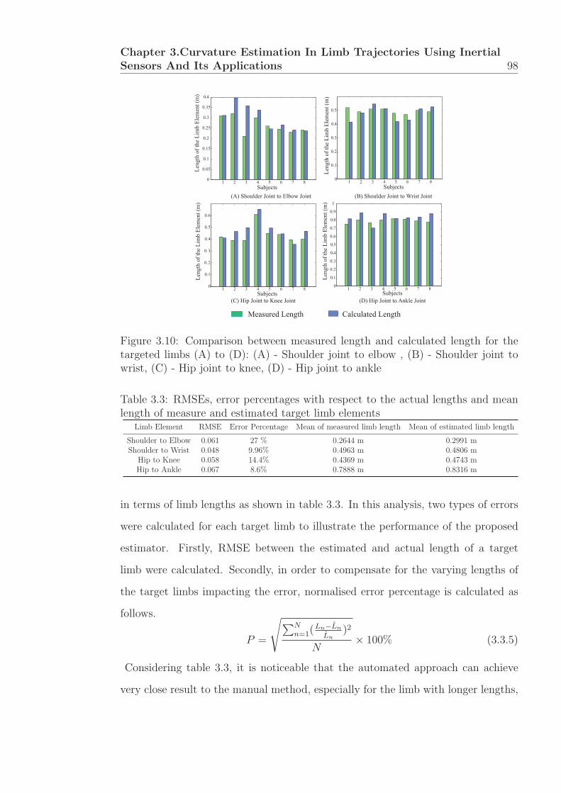
Chapter 3.Curvature Estimation In Limb Trajectories Using InertialSensors And Its Applications 98
1 2 3 4 5 6 7 80
0.05
0.1
0.15
0.2
0.25
0.3
0.35
0.4
SubjectsLe
ngth
of t
he L
imb
Elem
ent (
m)
(A) Shoulder Joint to Elbow Joint
1 2 3 4 5 6 7 80
0.1
0.2
0.3
0.4
0.5
Subjects
Leng
th o
f the
Lim
b El
emen
t (m
)
(B) Shoulder Joint to Wrist Joint
1 2 3 4 5 6 7 80
0.1
0.2
0.3
0.4
0.5
0.6
Subjects
Leng
th o
f the
Lim
b El
emen
t (m
)
(C) H Joint to Knee Joint
1 2 3 4 5 6 7 80
0.1
0.2
0.3
0.4
0.5
0.6
0.7
0.8
0.9
1
Leng
th o
f the
Lim
b El
emen
t (m
)
Subjects(D) H p Joint to Ankle Joint
Measured Length Calculated Length
Figure 3.10: Comparison between measured length and calculated length for thetargeted limbs (A) to (D): (A) - Shoulder joint to elbow , (B) - Shoulder joint towrist, (C) - Hip joint to knee, (D) - Hip joint to ankle
Table 3.3: RMSEs, error percentages with respect to the actual lengths and meanlength of measure and estimated target limb elements
Limb Element RMSE Error Percentage Mean of measured limb length Mean of estimated limb length
Shoulder to Elbow 0.061 27 % 0.2644 m 0.2991 mShoulder to Wrist 0.048 9.96% 0.4963 m 0.4806 m
Hip to Knee 0.058 14.4% 0.4369 m 0.4743 mHip to Ankle 0.067 8.6% 0.7888 m 0.8316 m
in terms of limb lengths as shown in table 3.3. In this analysis, two types of errors
were calculated for each target limb to illustrate the performance of the proposed
estimator. Firstly, RMSE between the estimated and actual length of a target
limb were calculated. Secondly, in order to compensate for the varying lengths of
the target limbs impacting the error, normalised error percentage is calculated as
follows.
P =
√∑Nn=1(
Ln−Ln
Ln)2
N× 100% (3.3.5)
Considering table 3.3, it is noticeable that the automated approach can achieve
very close result to the manual method, especially for the limb with longer lengths,

Chapter 3.Curvature Estimation In Limb Trajectories Using InertialSensors And Its Applications 99
such as shoulder to wrist and hip to ankle.
1 2 3 40.2
0.3
0.4
0.5
0.6
0.7
0.8
0.9
1
Limb elements
Mea
n Le
ngth
(m
)
Calculated lengthMeasured length
Figure 3.11: The mean value between measured length and calculated length: xaxis indicates the target limbs such as 1 - Shoulder to wrist, 2 - Shoulder to elbow,3 - Hip to ankle and 4 - Hip to knee
From table 3.3, shoulder to wrist was the most accurately estimated with RMSE
of 0.048 m and least percentage error could be observed in hip to knee target limb.
However, shoulder to elbow limb has the highest average percentage error (27%),
almost doubled compared to hip to knee, although the percentage error for the other
two limb segments were below 10%. This is mainly due to comparatively shorter
limb lengths considered. For an example, the average measured length of shoulder
to elbow is 0.2644 m and the estimated length is 0.2991 m. Though the absolute
error is only 0.0327 m, the percentage error reaches 23%. In comparison, though
the absolute error for hip to ankle is 0.0428 m, because the limb length is 0.7888
m, the percentage error is only 5.4%.
Considering RMSEs for each target limbs, the proposed approach with LNT
gives significantly accurate result with a low RMSE (approximately 0.06 m). How-
ever, a lesser percentage error (less than 15%) could be obtained for the longer limb
component such as hip to knee, hip to ankle and shoulder to wrist. Furthermore, the
mean length and standard deviation of each target limb segments were calculated
for the second analysis as shown in figure 3.10. The box plot shown in figure 3.11
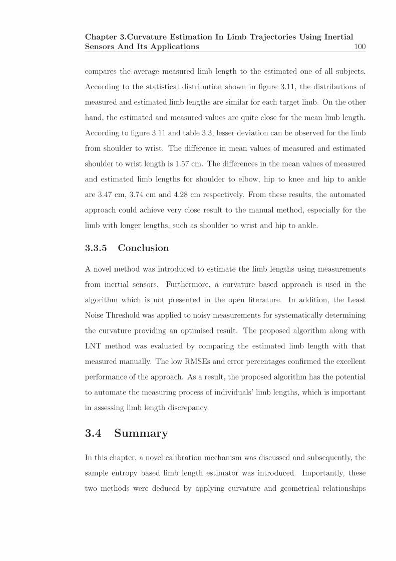
Chapter 3.Curvature Estimation In Limb Trajectories Using InertialSensors And Its Applications 100
compares the average measured limb length to the estimated one of all subjects.
According to the statistical distribution shown in figure 3.11, the distributions of
measured and estimated limb lengths are similar for each target limb. On the other
hand, the estimated and measured values are quite close for the mean limb length.
According to figure 3.11 and table 3.3, lesser deviation can be observed for the limb
from shoulder to wrist. The difference in mean values of measured and estimated
shoulder to wrist length is 1.57 cm. The differences in the mean values of measured
and estimated limb lengths for shoulder to elbow, hip to knee and hip to ankle
are 3.47 cm, 3.74 cm and 4.28 cm respectively. From these results, the automated
approach could achieve very close result to the manual method, especially for the
limb with longer lengths, such as shoulder to wrist and hip to ankle.
3.3.5 Conclusion
A novel method was introduced to estimate the limb lengths using measurements
from inertial sensors. Furthermore, a curvature based approach is used in the
algorithm which is not presented in the open literature. In addition, the Least
Noise Threshold was applied to noisy measurements for systematically determining
the curvature providing an optimised result. The proposed algorithm along with
LNT method was evaluated by comparing the estimated limb length with that
measured manually. The low RMSEs and error percentages confirmed the excellent
performance of the approach. As a result, the proposed algorithm has the potential
to automate the measuring process of individuals’ limb lengths, which is important
in assessing limb length discrepancy.
3.4 Summary
In this chapter, a novel calibration mechanism was discussed and subsequently, the
sample entropy based limb length estimator was introduced. Importantly, these
two methods were deduced by applying curvature and geometrical relationships

Chapter 3.Curvature Estimation In Limb Trajectories Using InertialSensors And Its Applications 101
of circular movements. Further, the inaccuracy due to misalignment of sensors
has been corrected which results improved accuracy for quantitative analyses using
inertial sensors.

Chapter 4
Qualitative Analysis Of HumanKinematics With Inertial Sensors
4.1 Introduction
In literature, computational methodologies for analysing human kinematics are ba-
sically divided into two categories [171] as follows.
1. Algorithms which partition the human kinematics through thresholds based
on experimental observations of sensor data [172, 173, 174]
2. Machine-learning schemes which extract patterns from large sensor datasets
based on certain assumptions [175, 176]
In the first category, several sensors are fused to derive deterministic information
(threshold) about human kinematics such as movement angle and limb length. In
the second category, the machine learning and statistical tests are applied to obtain
a qualitative information under a certain confidence level. Both of these analyses
are essential particularly for evaluating patients with certain neurological conditions
such as stroke and Parkinson’s disease. However, qualitative analysis is not univer-
sal as quantitative analysis, because the analysis usually depends on a number of
impact factors. As an example, the severity of a Parkinson’s patient is subjectively
determined based on several physical features such as slow movements, less flexi-
bility and rigidness. In such cases, the qualitative analyses are usually conducted
102

Chapter 4.Qualitative Analysis Of Human Kinematics With Inertialsensors 103
for determining severity of the disease. The observations are analysed applying
statistical and machine learning techniques to evaluate how well the given activities
are performed.
In this chapter, two major objectives were attempted to achieve using qualitative
analyses about human movements. the first objective is to investigate the feasibility
of statistically distinguishing the Parkinson’s patients and healthy subjects based on
sensor observations while conducting trunk movements. The main focus is analysing
three physical features of Parkinson’s patients such as slow movements, rigidness
and less flexibility of trunk based on thoracic movement and trunk rotation with
leg displacements. In this study, the thoracic rotation is referred the spine rotation
without leg displacements.
As the second objective, the relationship between energy consumption and gait
activities is investigated. The main challenge with this analysis is that the metabolic
relationship with energy and exercise level has number of influencing factors, such
as age, height, weight, fitness of the body and the nature of the exercise. Hence,
the derivation of the relationship between energy and a particular influencing fac-
tor is difficult. Furthermore, medical standard equipment for determining energy
consumption such as V O2 machines, evaluate overall energy consumption of the
complete human body rather than particular body movements such as gaits. Hence,
identifying the metabolic equation of energy consumption for gait exercises is chal-
lenging with this equipment. Additionally, they are not easy to use nor cost effective
and only suitable for laboratory environments [177].
The rest of this chapter is organized as follows: section 4.2.1 discusses the analy-
sis for trunk movements using inertial sensors. In this section, statistical techniques
have been applied to distinguish the Parkinson’s patient and healthy subjects based
on the underlined physical features. Section 4.3 introduces ambulatory energy ex-
penditure evaluation for several level of treadmill exercises from walking to running
with the aid of inertial sensors. Section 4.4 concludes the chapter.

Chapter 4.Qualitative Analysis Of Human Kinematics With Inertialsensors 104
4.2 Investigation of the thoracic rotational pat-
terns of Parkinson’s patients using inertial
sensors
Parkinson’s disease (PD) is a chronic, progressive and degenerative disorder of the
central nervous system [178] as discussed in section 1.4. A high percentage (52-62%)
of people with Parkinson’s disease have difficulty when turning [179], which is often
associated with falling and freezing of gait [180, 181]. This indicates a significant
negative effect on their quality of life [181]. Hence, it is important to analyse key
elements such as maximum span of turning, duration for turning and turning quality
in order to evaluate a Parkinson’s patients. In addition, if these assessments can be
carried out at home, this would be an affordable and cost saving solution than the
current practice which requires patients to attend clinics.
Some of the key clinical features of Parkinson’s patients are described as bradyki-
nesia, rigidity, tremor and postural instability. As a result, a patient’s movement
may slightly differ compared to a healthy person, particularly during standing, lo-
comotion and trunk movements [182]. Parkinsonian gait has various typical charac-
teristics such as a low walking velocity, small stride length, propulsion, retropulsion,
shuffling steps, reduced or absent arm swing and rigidity in trunk movements [182].
The Parkinson’s patients usually show difficulties while performing multi axial body
rotations. One such critical movement is trunk rotation, which changes the trunk
from the sagittal to transverse axis during locomotion [182].
According to Richard et al. 1999 [183], systematic manipulation of velocity
can be used to identify the coordination deficits and rigidity in trunk movement of
Parkinsons patients. This is believed to be a sensitive measure for early diagnosis
of Parkinson’s patients in pharmacological therapy [183]. According to studies of
Van Emmerik et al. in 1993, Wagenaar et al. in 1994 and Pei-Yi Chou et al.
in 2013, difficulties in trunk movement of Parkinson’s patients has been shown in
gait initiation and switching gaits. Knuttson at al. 1972, and Murray et al. 1978

Chapter 4.Qualitative Analysis Of Human Kinematics With Inertialsensors 105
recognised two major characteristics of a Parkinson’s patient such as lower velocity
during movement and rigidity of the trunk.
MEMS sensors are more accurate and less noisy for movements having low ac-
celerations and velocity. Usually Parkinson’s patients have slow movements. Hence
these sensors can be used to capture and monitor kinematics of Parkinson’s patients
especially to identify trunk moving patterns compared to healthy people. However,
tremor is a natural property of Parkinson disease which cannot be avoided or reset.
G Buzsaki et al. [184] has suggested that the tremor of Parkinson’s disease has
a systematic rhythm and this systematic rhythm can be removed. Hence, this is
unlike to have any substantial impact in the analysis on their natural movement
patterns.
4.2.1 Evaluation of physical features of Parkinson’s patients
In this section, two movement disorders of Parkinson’s patients are investigated.
4.2.2 Experiement setup
In the clinical study, a specifically designed jacket as shown in figure 4.1 is used.
Initially, the jacket was designed with 13 pockets to accommodate BioKin inertial
sensors. A stretchable fabric was used to ensure the tightness between the fabric
and body surface.
Two following exercises were conducted while wearing the jacket.
1. Turning the body with leg displacements (Refer figure 4.2 (a) and (c))
2. The trunk rotation (Refer figure 4.2 (a) and (b))
In the turning body exercise with leg displacements, sensor 5 and 9 were used
to analyse kinematics of the spine. Firstly, three healthy subjects were asked to
turn their body by 90 degrees, as shown in figures 4.2(a) and 4.2(c) without foot
displacements and secondly, to turn their body by 90 degrees having steps imitating
the Parkinson’s patient as figures 4.2(a) and 4.2(b).

Chapter 4.Qualitative Analysis Of Human Kinematics With Inertialsensors 106
Sensor 1 Sensor 2
Sensor 3 Sensor 4
Sensor 5
Sensor 6 Sensor 7
Sensor 8
Sensor 9
Sensor 10
Sensor 11
Sensor 12
Sensor 13
Figure 4.1: Sensor suite having 13 sensor positions
(a) (b) (c)
Figure 4.2: Exercise 1: (a) and (b) are the initial posture and end posture of thoracicrotation, (a) and (c) are the initial posture and end posture of body rotation withleg displacements
The second exercise is designed to evaluate the trunk movements while perform-
ing a pointing test as shown in figure 4.3. Four sensors (Sensor 1, Sensor 2, Sensor 3
and Sensor 4 of the jacket) were used to make it more convenient to patients (refer
to figure 4.1). This analysis was conducted with eight healthy controls and sev-
enteen Parkinson’s patients. All the subjects were between 40-60 years old. Each
subject was positioned in the centre of a room and the two markers were attached
on both sides (left and right) of the wall. The subject was then asked to point to

Chapter 4.Qualitative Analysis Of Human Kinematics With Inertialsensors 107
(a) Start (b) End
Figure 4.3: Pointing exercise
each marker alternatively with thoracic rotation but without leg displacement.
4.2.3 Results and discussion
Distinguishing upper body kinematics: Thoracic rotation with and with-out leg displacements
The gyroscope rates were analysed for two scenarios: 1. Thoracic rotation (Refer
figure 4.4 ) and 2. Body rotation with leg displacements (Refer figure 4.5).
Figure 4.4: Angular rates for thoracic rotation
From figures 4.4 and 4.5, The moving pattern was clearly observed that can be
used to differentiate the thoracic rotation and the body rotation having leg dis-
placements. Fast Fourier Transform (FFT) technique was applied to both datasets

Chapter 4.Qualitative Analysis Of Human Kinematics With Inertialsensors 108
Figure 4.5: Angular rates for rotation with steps
to distinguish thoracic rotation from the body rotation with leg displacements. Fre-
quency spectrums were obtained from the FFT analyses of angular rates observed
in two scenarios. Several peaks could be observed in the frequency spectrum of the
body rotation with leg displacements as shown in figure 4.6(b). For the thoracic
rotation without leg displacements, these peaks were not evident in the frequency
spectrum, as shown in figure 4.6(a).
(a) Thoracic rotation (b) Turning body havingleg displacements
Figure 4.6: Frequency spectrum after applying FFT technique
Additionally, the gradient based statistical method was applied to differentiate
the kinematic artefacts of the two exercise scenarios. These two activities could
be distinguished by calculating the gradient of the movement angle at each sample

Chapter 4.Qualitative Analysis Of Human Kinematics With Inertialsensors 109
time. The gradient derived from the integrated angle of the thoracic movement,
was negative at each sample time, as shown in figure 4.7(a). Time varying sign of
gradient for the rotation with leg displacement could be observed as shown in figure
4.7(b).
(a) Thoracic rotation (b) Turning body having leg displace-ments
Figure 4.7: Gradient analyses of angular rates
According to the experimental results of the FFT technique and gradient based
method, the thoracic movement was successfully distinguished from the turning
the body with leg movements. Additionally, according to the frequency spectrums
generated by FFT, these two activities belong to different frequency domains.
Upper trunk movement without leg displacements
Trunk movements were further investigated based on the pointing exercise, as shown
in figure 4.3. The angular rates acquired from sensor 2 and sensor 4 (refer to figure
4.1) were processed in following forms.
1. Average maximum magnitude in angular rates acquired from sensor 2 and
sensor 4
2. Relative difference of magnitude in angular rates between sensors worn on
upper and lower body of trunk on the same side
3. Average maximum span (movement angle) of the hip

Chapter 4.Qualitative Analysis Of Human Kinematics With Inertialsensors 110
4. Relative difference of maximum span (movement angle) between sensors worn
on upper and lower body of trunk on the same side
A similar pattern in the above forms of data series could be seen in both healthy
subjects and Parkinson’s patients as shown in figure 4.8.
0 5 10 15 20 25 30
0
50
100
Time/(s)
w/(d
eg/s
)0 5 10 15 20 25 30
0
50
100
Time/(s)w/
(deg
/s)
Parkinson PatientHealthy Subject
0 5 10 15 20 25 30
0
10
20
30
50
/(deg
/s)
Time/(s)
w
0 5 10 15 20 25 30
0
20
Time/(s)
q/(de
g)
0 5 10 15 20 25 30
01020
Time/(s)
q/(de
g)
0 5 10 15
0
50
100
(A) Angular rates in Sensor 2Time/(s)
w/(d
eg/s
)
0 5 10 15
0
50
100
Time/(s)
w/(d
eg/s
)
0 5 10 15
0
20
100
/(deg
/s)
w
Time/(s)
0 5 10 15
020
(D) Movement Angle in Sensor 2Time/(s)
q/(de
g)
0 5 10 15
0
50
Time/(s)
q/(de
g)
(F) Angular rates in Sensor 2
(G) Movement Angle in Sensor 2
Figure 4.8: Comparison of healthy subjects and Parkinson’s patients
In order to distinguish the healthy subject and Parkinson’s patients, these data
series measured from gyroscope were further investigated based on two physical

Chapter 4.Qualitative Analysis Of Human Kinematics With Inertialsensors 111
features. The first physical feature under the consideration was execution speed
of movements. For this, the average cycle time and average magnitude in angular
rates for each pointing cycle were calculated. Figure 4.9 shows the statistical result
of analysing average relative magnitude. The averaged relative magnitude values
for eight controls and seventeen Parkinson’s patients are shown as in figure 4.9(a).
In general, the higher mean value is for healthy subjects than the patients, but the
variance for heathy subjects and patients are very similar according to table 4.1.
Figure 4.9(b) shows the variance of each subject as a box plot.
Table 4.1: The result of averaged relative magnitude in angular rates
Mean Standard Deviation
Healthy Subjects 67.08 degs−1 20.71 degs−1
Parkinson’s Patients 45.91 degs−1 20.8 degs−1
10
20
30
40
50
60
70
80
90
100
51 432 106 987 11 141312 15 16 191817 20 21 242322 25
Normal Patient
Rel
ativ
e A
ngul
ar ra
tes
(deg
/s)
Varia
nce
of H
ealth
y Su
bjec
t
Varia
nce
of P
atie
nts
(a) Magnitude in angular rates
0
20
40
60
80
100
120
Rel
ativ
e A
ngul
ar ra
tes
(deg
/s)
51 432 106 987 11 141312 1516 191817 20 21 242322 25
Normal Patient
Varia
nce
of H
ealth
y Su
bjec
t
Varia
nce
of P
atie
nts
(b) Variance in angular rates
Figure 4.9: Magnitude in relative movement based on angular rates of a cycle
Figure 4.10 shows the results of analysing cycle time in the pointing exercise.
The cycle time is referred to as the time for pointing from one marker to another and
pointing back to previous marker. According to figure 4.10(a), the mean value of
cycle time for Parkinson’s patients is higher than healthy subjects. This means that
healthy subjects finish the pointing cycle in a shorter time duration than patients.
However, the variance of patients is approximately three times higher than healthy
subjects according to table 4.2. Figure 4.10(b) shows the variance of each subject
in a box plot.

Chapter 4.Qualitative Analysis Of Human Kinematics With Inertialsensors 112
Table 4.2: The result of averaged cycle time of pointing cycle
Mean Standard Deviation
Healthy Subjects 2.67 seconds 0.38 secondsParkinson’s Patients 3.41 seconds 1.38 seconds
1.5
2
3
4
5
6
Cyc
le T
ime
(s)
51 432 106 987 11 141312 15 16 191817 20 21 242322 25
Normal Patient
Var
ianc
e of
Hea
lthy
Subj
ect
Varia
nce
of P
atie
nts
(a) Cycle time
1
2
3
4
5
6
7
Cyc
le T
ime
(s)
51 432 106 987 11 141312 1516 191817 20 21 242322 25
Normal Patient
Varia
nce
of H
ealth
y Su
bjec
t
Varia
nce
of P
atie
nts
(b) Variance in cycle time
Figure 4.10: Cycle time of a pointing cycle
The second physical feature is the relative maximum span between the upper
trunk and the lower trunk. The eight healthy subjects and twenty patients par-
ticipated in this analysis. The integrated movement angles for each pointing cycle
were calculated using gyroscope readings acquired from two sensors worn on upper
trunk and lower trunk of left side of the trunk. Then, the difference in movement
angles between upper trunk and lower trunk is the relative maximum span for the
cycle. To avoid the impact of gyroscope drift, the averaged relative maximum span
for all cycles is considered. Figure 4.11 shows the averaged relative maximum span
for all subjects.
Table 4.3: The result of averaged relative maximum span
Healthy subject Parkinson’s Patient
Average maximum span of upper trunk 49.50 degrees 41 degreesAverage maximum span of lower trunk 48 seconds 27.88 seconds
Relative average maximum span 28.66 degrees 16.67 degreesStandard deviation of relative span 17.89 degrees 18.61 degrees
According to the experimental results as shown in table 4.3, the healthy subject
has a larger span for both upper body and lower body compared to Parkinson’s

Chapter 4.Qualitative Analysis Of Human Kinematics With Inertialsensors 113
Rel
ativ
e A
ngle
(deg
)
5432 6 987 242322 25 2726 28
Normal Patient
Varia
nce
of H
ealth
y Su
bjec
t
Varia
nce
of P
atie
nts
Figure 4.11: Comparison of relative orientation between upper trunk and lowertrunk
patients. Similarly, the relative average maximum span between upper body and
lower body is relatively higher for a healthy subject than a Parkinson’s patient. The
relative span for a healthy subject is approximately twice compared to a Parkinson’s
patient. This implies that the Parkinson’s patient has less flexibility in the trunk
compared to a healthy person. The standard deviation in both healthy subjects’
and patients’ relative span are approximately similar.
According to above analyses, the author can conclude that Parkinson’s patient
has less flexibility to move both upper trunk and lower trunk independently because
they have less relative span than a healthy subject. Further, Parkinson’s patients
move slower than healthy subjects since the patients’ cycle time is approximately
21% less than a healthy person’s cycle time.
Analysis combining multiple features
In this section, each patient is investigated based on two of above identified physical
features in the pointing exercise. The combinations of physical features are as
follows.
1. Cycle time and relative averaged maximum span of a cycle
2. Cycle time and relative average maximum magnitude in angular rates of a
cycle
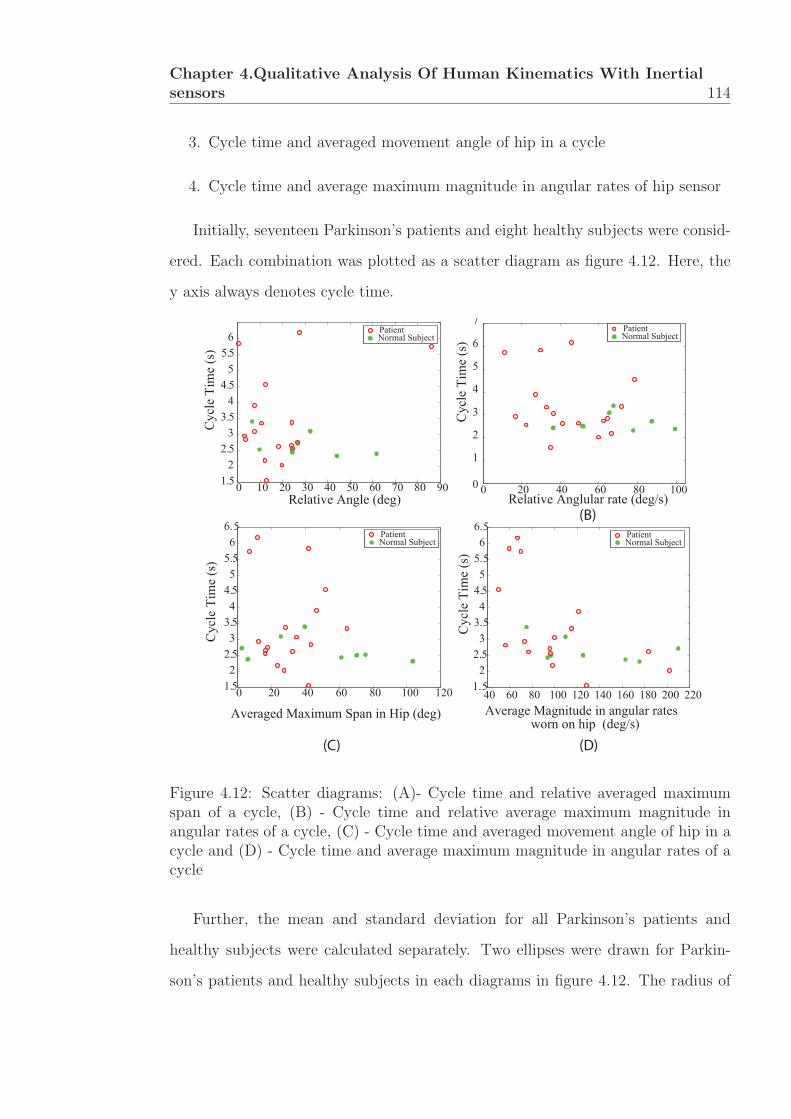
Chapter 4.Qualitative Analysis Of Human Kinematics With Inertialsensors 114
3. Cycle time and averaged movement angle of hip in a cycle
4. Cycle time and average maximum magnitude in angular rates of hip sensor
Initially, seventeen Parkinson’s patients and eight healthy subjects were consid-
ered. Each combination was plotted as a scatter diagram as figure 4.12. Here, the
y axis always denotes cycle time.
0 20 40 60 80 1000
1
2
3
4
5
6
7
Relative Anglular rate (deg/s)
Cyc
le T
ime
(s)
Averaged Maximum Span in Hip (deg)
Cyc
le T
ime
(s)
Average Magnitude in angular rates
Cyc
le T
ime
(s)
worn on hip (deg/s)(D)(C)
(B)
0 10 20 30 40 50 60 70 80 901.52
2.53
3.54
4.55
5.56
Relative Angle (deg)
Cyc
le T
ime
(s)
PatientNormal Subject
PatientNormal Subject
40 60 80 100 120 140 160 180 200 2201. 5
22. 5
33. 54
4. 55
5. 56
6. 5
PatientNormal Subject
0 20 40 60 80 100 1201. 52
2. 53
3. 54
4. 55
5. 56
6. 5
PatientNormal Subject
Figure 4.12: Scatter diagrams: (A)- Cycle time and relative averaged maximumspan of a cycle, (B) - Cycle time and relative average maximum magnitude inangular rates of a cycle, (C) - Cycle time and averaged movement angle of hip in acycle and (D) - Cycle time and average maximum magnitude in angular rates of acycle
Further, the mean and standard deviation for all Parkinson’s patients and
healthy subjects were calculated separately. Two ellipses were drawn for Parkin-
son’s patients and healthy subjects in each diagrams in figure 4.12. The radius of

Chapter 4.Qualitative Analysis Of Human Kinematics With Inertialsensors 115
ellipse was the standard deviation in corresponding axes. The centre of the ellipse
is the coordinations of the mean value of Parkinson’s patients or healthy subjects.
With this representation as shown in figure 4.13, the patients and healthy subjects
could be classified.
CycleTime(secon
ds)
Relative Angle (deg)CycleTime(secon
ds)
Relative Magnitude in Angular rates (deg/s)
CycleTime(secon
ds)
Average Maximum Span in Hip (deg)
(A) (B)
(C)
CycleTime(secon
ds)
Average MaximumMagnitude in Angular Rates worn on Hip (deg/s)(D)
Figure 4.13: Classification between healthy subjects and patients: (A)- Cycle timeand relative averaged maximum span of a cycle, (B) - Cycle time and relative aver-age maximum magnitude in angular rates of a cycle, (C) - Cycle time and averagedmovement angle of hip in a cycle and (D) - Cycle time and average maximummagnitude in angular rates of a cycle
According to the result as in figures 4.13, figure 4.13 (B) has classified patients
(red region) and healthy subjects (green region) with least overlapping of two re-
gions. The second least overlapped representation is figure 4.13 (D). This implies
that angular rates without processing gives a more accurate classification than other
process factors such as integrated angle.

Chapter 4.Qualitative Analysis Of Human Kinematics With Inertialsensors 116
Figures (C) and (D) of 4.13 are processed based on angular rates measured from
sensors worn on the hip. Here, the possibility to reduce sensor usage is investigated
in these tests in order to make it more convenient for the patients. According to
results, figure (D) has less overlapped regions than figure (A), which means that
the angular rates from a sensor worn on hip is represented in two groups than the
processed relative angle using two sensors.
4.2.4 Summary
The qualitative analyses can be used evidently to distinguish the Parkinson’s pa-
tients from healthy subjects based on upper body kinematics. In this study, three
important physical features of Parkinson’s patient such as rigidness, reduced flex-
ibility and slower movements could be qualitatively distinguished using gyroscope
readings from the IMU that was attached on the back of the trunk.
However, one of challenges associated with these analyses is the larger variance
which makes it difficult to separate the two groups as Parkinson’s disease affected
and non-affected. The reason behind this difficulty is the level of Parkinson’s dis-
ease severity of each patients and healthy subjects with back pains (not due to
Parkinson’s disease). Some of patients are close to healthy subject in functionality
aspects. Hence, further investigations should be conducted to obtain more accurate
classification of patients from healthy subjects on their physical features.
Subjects were evaluated based on several mutual physical features to classify
the Parkinson’s patients and healthy subjects. Under these analyses, this approach
could be statistically distinguished that Parkinson’s patients and healthy subjects
based on cycle time and relative average maximum magnitude in angular rates of
a cycle.

Chapter 4.Qualitative Analysis Of Human Kinematics With Inertialsensors 117
4.3 Ambulatory energy expenditure evaluation for
gait exercises
Walking and running are identified as two crucial exercises in human locomotion,
hence numerous studies were conducted under these two categories typically using
a treadmill, such as Andriacchi et al. in 1977, Larsson et al. in 1980, Wagenaar
and Beek in 1992 and Emmerik and Wagenaar in 1996. Parallel to treadmill based
research, a number of studies were conducted to suggest transition in the frequency
relations between the arms and the legs in the bipedal walking mode, such as Craik
et al. in 1976, Wagenaar and Van Emmerik in 1994. A number of studies also
used inertial sensors for analysing gait patterns. Seven T. Moore et al. in 2006,
Benoit Mariani et al. in 2010, Rahimi F. in 2011 and Weijun Tao et al. in 2012
investigated gaits patterns and switching gaits using body worn sensors. Inertial
sensors have been used to obtain the main gait characteristics such as stride length
and gait cycle time [185]. In sports science, the measurement of how much energy
someone has expended through exercise is recognized as a hard problem to solve.
A common form of exercise that would involve energy estimation is walking.
This enabled an easy scenario for capturing the gyroscope data from the movement
of legs using IMU. Knowing this, the experiment performed with healthy subjects
between the ages of 20 to 45 and were on a treadmill at various speeds for some
time for each speed. The BioKin system, and an oxygen intake measurement device
were used to measure limb movement and oxygen consumption levels. Using the
data collected, a correlation was sought and a linear model derived so that energy
estimation for running or similar activities could be measured accurately using an
angular speed ratio based device in place of a bulk oxygen consumption system.
The rate of energy expenditure of a person who is moving (e.g. walking or
running) is linearly proportional to their velocity [186]. Inertial data acquisition
is prone to errors but as a first step to gaining energy expenditure information
[187], the system utilizes a single tri-axial accelerometer and is called the Move II

Chapter 4.Qualitative Analysis Of Human Kinematics With Inertialsensors 118
sensor. In the experiment, which comprised three different walk speeds on a tread
mill, the step cycle or two consecutive steps were interpreted and converted the
signal to a feature vector using weight and height as parameters to influence energy
expenditure measurement. One restriction is that it is indoor based and does not
have any GPS based sensors to measure outside movements. Steps using a sensor
placed on the chest in [188] utilized a full angular speed ratio unit that comprised of
accelerometer, gyroscope and magnetometer (although the former two were used).
The same issue was raised in [189] where a sensor using an angular speed ratio, albeit
a different model from [187], was placed on the hip. [189, 190, 191, 192, 193] found
that utilising acceleration and rotation data as well as using a V O2 breath sensor
apparatus to confirm energy measurement was accurate in some combinations but
not others. Vathsangam et al. investigated this further, using statistical analysis
to gain a better understanding of the results. Specifically, it was found that the
combination of both acceleration and gyroscope data yielded the least amount of
error.
It was evident from the paper that a different implementation of energy mea-
surement capture was presented. A new approach was looked at in [194] and [195],
where the angle of the knee was taken by using gyroscopes on two sensors on the
leg, where one would be on the knee and other positioned on the lower leg, and
the results were then used to estimate energy levels. In both papers, the aim is to
verify that using knee angle measurements is reliable, not to observe energy expen-
diture. It should be noted that all of the papers surveyed looked at indoor walking
whilst [189] also considered outdoor walking using a GPS system. Walking can be
considered a common enough activity that should be used for the purposes of gait
analysis and energy expenditure measurement and is easy to model.
In [189, 190, 191, 192, 193], the authors constantly used Bayesian Linear Re-
gression and Gaussian Process Regression throughout their experiments as well as
coupling both gyroscopic and acceleration measurements. In [189], the authors used

Chapter 4.Qualitative Analysis Of Human Kinematics With Inertialsensors 119
Hierarchical Linear Models. This was used to supplement the energy expenditure
estimation model by looking at the variations from user to user. It includes the
user’s height, weight, and age as parameters for the model as inputs. From this, a
gap in the literature covered was found, and taking the experiment from [194] and
[195] and instead of using the knees - it was found that using the angular velocity
of the legs could be used to measure energy expenditure.
4.3.1 Energy expenditure in activities
The gold standard in evaluating the energy expenditure in a human body is by
means of a metabolic measurements system [196]. A metabolic measurement system
measures the consumption of Oxygen through a breathing mask attachment, as
illustrated in figure 4.14. Energy expenditure from the rate of oxygen consumption
data is calculated using(4.3.1) [197]:
Em =vo × 20900
60(4.3.1)
where vo represents the oxygen consumption during the activity in l/min and en-
ergy rate that is being measured Em is in watts. The energy calculation from IMU
does not have a direct relationship with energy expenditure via a rate of change of
limb angles. The major disadvantage in such a system is the inability to measure
energy or activity level while the subject is at rest or performing non-mobile exer-
cises whereas the metabolic measurement systems can measure energy expenditure
during any activity. Therefore, this study is focused on measuring energy expendi-
ture in walking and running based activities where the subject’s activity level has
a close relationship with the movement intensities of body segments.
In this study, angular rates of the lower limb has been used to estimate the
energy expenditure during the activity as follows:
Er =k
T
∑(‖ω‖2) . (4.3.2)
Here T is the duration of the activity in seconds, energy rate of the activity
level Er is in watts, ω = [ ωx ωy ωz ] represents the raw gyroscope measurements

Chapter 4.Qualitative Analysis Of Human Kinematics With Inertialsensors 120
around the respective local coordinate axis from the ankle mounted sensor (see
figure 4.14(b)) and k is a scalar function to transform the angular rates into the
energy. This equation assumes a linear relationship between mean of ‖ω‖2 and the
actual energy expenditure, which will be confirmed later.
Another method to evaluate energy in walking or running based exercises is
based on the assumption that the energy consumption is linearly proportionl to
the speed of walking or running [186]. The following empirical formula has been
employed in calculating energy using speed of motion,
Es =(vL ×m)
1000, (4.3.3)
where vL represents the linear velocity of motion (i.e. the treadmill speed),
energy rate of the activity level Es is in watts and m represents the weight of the
subject in kilograms. This provides the Es in the rate of oxygen consumption which
can be used with equation (4.3.1) to calculate the actual energy consumption inW .
4.3.2 Experiment setup
The experiment was conducted in a laboratory environment with a speed regulated
treadmill for precise control of the activity intensity. The experiment was performed
with six subjects (five males and one female) without any history of orthopaedic
or intramuscular impairments. All subjects were non athletes and recruited from
general population within the age bracket of 20 to 45 years.
The oxygen intake measurement system was the Metamax 3B unit developed
by Cortex-Medical. Time-stamped metabolic information was stored in the device
and was later transferred to a computer for analysis.
Inertial measurements, in particular the angular speed of the limb which is of
interest to this study, were recorded using BioKin sensor attached to ankle of the
subject as shown in figure 4.14(b).
The activity level of the experiment was controlled by means of the speed of
the treadmill the subject is walking/running. Before the exercises, the subject’s

Chapter 4.Qualitative Analysis Of Human Kinematics With Inertialsensors 121
(a) Experimental setup (b) Sensor worn Leg
Figure 4.14: (a)- Experimental Setup: Metamax metabolic measurement systemwas attached to the subject while performing the treadmill based exercises. (b) -Capturing inertial data: BioKin-WMS inertial measurement sensor was attachedto the subject’s ankle while performing the treadmill based exercises.
metabolic rate was measured for the resting state. This parameter was used to
calibrate the Metamax system as well as to obtain a baseline measurement for the
subject. However, in the inertial measurement system, the resting state does not
provide any valuable information, hence this was normalized by means of normal-
izing against the first activity level, as explained in the next section.
Each subject was asked to perform walking/running activities for five activity
levels at treadmill speeds 3, 5, 7, 9 and 11km/h with each activity lasting for 2 min-
utes. The length of time is comparatively short compared to [191] but the duration
is long enough to get valid sets of data for each speed section (see [197]). The
V O2 measurements were taken in the final minute of recording. In addition to the
logging of gyroscope, accelerometer and rate of oxygen consumption measurements,
height and weight were measured in order to use older models/equations to roughly
estimate their energy expenditure.
In this study, the author aimed at develop a relationship between the energy
expenditure from a gold standard metabolic measurement system and the proposed
energy expenditure system introduced in equation (4.3.2). The system uses angular
rate measurements recorded by an IMU sensor worn on the ankle. The subject
was investigated based variation of the energy expenditure relationships estimated

Chapter 4.Qualitative Analysis Of Human Kinematics With Inertialsensors 122
0 1 2 3 4 50
1
2
3
4
5
Limb angular rate based energy ratio (ψr)M
etab
olic
rate
bas
ed e
nerg
y ra
tio (ψ
m)
Mean data for five subjectsLeast Square LineEvaluation data for the sixth subject
Figure 4.15: Variation of treadmill speed derived, normalized energy expenditure(ψr) with activity levels for all test subjects
with different methods. An additional energy expenditure estimation method was
employed using speed of walking or running as introduced in equation (4.3.3). Note
that during the treadmill based exercises, some subjects could not perform the full
set of activity levels due to physical fitness level of the individual.
4.3.3 Relationship of gyro based proposed energy expendi-ture with gold standard metabolic rate
In this section, the proposed energy expenditure technique was compared as (4.3.2)
with the gold standard oxygen consumption based system. In order to maintain gen-
erality and comparability between two energy expenditure calculation techniques,
the normalized energy expenditure compared to the first level of activities, i.e.
3km/h walking was used in this study. The normalized energy at ith activity level
is calculated as,
ψi =Ei
E1
. (4.3.4)
Here, E1 is the energy for the base activity level of 3km/h walk and Ei is the
estimated energy at ith activity level. The mean energy across five subjects for
each activity level was calculated and figure 4.15 illustrates the comparison of this
approach with gold standard. A linear regression line was generated using least-
square approximation of the data points and the linear relationship was evaluated

Chapter 4.Qualitative Analysis Of Human Kinematics With Inertialsensors 123
using the sixth subject data. The evaluation data set demonstrated a mean error
of −0.0959 with a standard deviation of 0.2306. The proposed hypothesis in this
study to explain such high standard deviation is the subject specific variation of
the energy expenditure calculation from each method. In order to evaluate this
hypothesis, the data for each subject was analysed to derive a pattern, as shown in
the next section.
4.3.4 Variation of energy expenditure pattern with the sub-ject
The variations in the normalized energy-activity level relationship within each sub-
ject were investigated. The energy expenditure calculated from each method were
evaluated in section 4.3.1 and are shown in Fig. 4.16(a), 4.16(b) and 4.16(c).The
normalized energy-activity level is represented as a ratio ψi with ψr being the ratio
of limb based movements, ψm is V O2 based Energy Expenditure and ψs is running
or walking speed. The idea of using a ratio is useful as it allows us to see these
variations from an objective viewpoint and allows the observation of abnormalities
from what happens in the individual ψs, ψm and ψr readings in a unitless context.
Essentially, the walking/running speed based energy estimation ratio ψs does not
demonstrate any difference among the subjects due to the fact that ψs only de-
pends on the speed and does not take any physical parameter of the subject into
the equation. However, metabolic rate and lower-limb angular rate based energy
estimation techniques demonstrates a clear variation between the subjects. This
variation could be from the varying weight and height of each subject, with Body
Mass Index (BMI) seemingly affecting the V O2 Max of those who run/walk as ob-
served in [198]. Therefore, further study will need to be performed with more test
subjects in order to confirm if these two variables can be attributed to be an influ-
ence on the final results and then possibly define the relationship between energy
estimation and a person’s BMI.
It should be noted that subject 4 and 5 did not complete the run, with subject

Chapter 4.Qualitative Analysis Of Human Kinematics With Inertialsensors 124
(a) (b)
(c)
Figure 4.16: (a)- Variation of rate gyro derived, normalized energy expenditure (ψr)with activity levels for all test subjects, (b)- Variation of metabolic measurementbased, normalized energy expenditure (ψm) with activity levels for all test subjects,(c)- Variation of treadmill speed derived, normalized energy expenditure (ψs) withactivity levels for all test subjects
4’s V O2 result was not recorded in the final activity level. Subject 5 found the
ambulation at the intensity level was too uncomfortable and had to discontinue
that part of the experiment.
4.3.5 Summary
In this study, the feasibility of employing a single inertial sensor based energy
expenditure estimation technique were investigated for treadmill based exercises.

Chapter 4.Qualitative Analysis Of Human Kinematics With Inertialsensors 125
Although the author have limited the study to treadmill based exercises, to main-
tain a controlled experimental setup the same technique could be used in out-door
walking and running based exercises. The proposed energy estimation method was
evaluated with the industry standard Metamax metabolic rate measurement sys-
tem, which is the gold standard form of measurement in human energy expenditure.
4.4 Conclusion
The investigation of human movements are usually conducted as two types of anal-
yses: deterministic and qualitative analyses. The use of inertial sensors for deter-
ministic analyses was investigated in chapter 2 and chapter 3. In this chapter, the
main focus was to investigate the possibility to use inertial sensors in qualitative
analyses which are very important for qualitative evaluations of human movements.
The trunk movements and gait analyses were investigated under this form of ap-
proaches. The feasibility of separating Parkinson’s patients and healthy patients
were investigated based on three physical features such as rigidness, flexibility and
execution speed of movements based on trunk movements using gyroscope readings.
Further, the relationship between energy expenditure for ambulatory exercises was
analysed using angular rates and accelerometer readings. The author confirmed a
linear relationship with energy and activity levels in line with common understand-
ing in literature. All these analyses demonstrates that the IMU sensors can be used
to perform qualitative analyses of human movements.

Chapter 5
Mobile - Cloud Based PhysicalTele-rehabilitation System - APrototype
5.1 Introduction
The severe challenges in rehabilitation such as skyrocketing healthcare expenditure
and increasing aged population highlight the need for innovative solutions sup-
porting more accurate, affordable, flexible and personalized medical diagnosis and
treatments [199]. This implies that the unnecessary cost components should be
avoided while providing convenient and more facilities to patients. As in [199], the
critical and costly part of current healthcare systems is the frequently monitoring of
patients signs and other physiological signals, which can be mitigated with the aid
of long-term, off-site or in-home care health systems. Through in-home care [199],
it is possible to save time and money for both caregivers and patients, providing
greater convenience to patients at the same time.
Furthermore, mobile phone based, domestic medication is popular due to easy
access and higher availability. Recent advances in wireless body sensors and mobile
technologies have promoted the use of mobile-based health monitoring and alert
systems (usually referred as mHealth) [199]. However the usage of mobile phone,
in-home based medications is limited due to its inherent constraints such as less
126

Chapter 5.Mobile - Cloud Based Physical Tele-rehabilitation System -A Prototypes 127
memory, limited processing power, battery power and screen size [200]. Still, mo-
bile phones are popular for medical monitoring and recently, mobile-based medical
monitoring devices have been developed with the ability to process a wide variety
of classes of physiological signals [199, 201, 202].
This chapter attempts to propose a novel cloud based architecture of a biomed-
ical system for a wearable motion kinematic analysis system using IMU devices
which mitigates the above mentioned deficiencies of mobile devices. Furthermore,
novel multilevel data encoding scheme is proposed satisfying the limitations in mo-
bile cloud computing devices such as battery power and computational cost. An-
other advantage of this scheme is that different sensory devices can be connected
together for deriving better information. the introducing platform is usable not
only for patients to experience tele-rehabilitation services but also for therapists to
acquire essential support from analysis oriented decision support system (AODSS)
for making decisions on treatments after conducting extensive analyses. Further,
the safety issues and solutions are addressed in underlined tele-rehabilitation system
for reliable service.
5.2 Available remote human monitoring system
and architectures
Cloud and mobile technologies are widely used in various fields such as bio-medical
[199, 203] and sport activity monitoring [199, 203]. The studies in [199, 203] pre-
sented a mobile phone based system, which was enabled with features to acquire
various physiological signals from a set of ambient body sensors. The system per-
formed the regular lightweight and on-site diagnostic tasks using cloud technology
by executing heavy algorithms on diverse devices such as smart phones, laptops,
tablets, hospital servers and video conferencing tools. Importantly, their architec-
ture is fully reliant on a cloud service. It has monitored the abnormalities of patients
and capable of raising diagnostic alarms for medical staffs when necessary.

Chapter 5.Mobile - Cloud Based Physical Tele-rehabilitation System -A Prototypes 128
The Mobile Cloud Computing(MCC) is an emerging technology in computing.
The one advantage using MCC model in medical domain is that the data intensive
analyses from the medical applications can be executed in one system rather than
number of dedicated analysing systems [73]. The second advantage is that the
data acquired from medical systems can be stored in a private or hybrid database
servers according to privacy needs. Third advantage is that the most of cloud
services provides relational database management services (RDBMS) as their web
service, since most of developers are familiar with RDBMS. Additionally, the fast,
flexible and comprehensive analyses can be performed by extracting the appropriate
datasets from systems using pre-processed MATLAB scripts and stored the results
in different formats such as PDF and JSON.
The case study in [204] presented a biometric evaluation system on the cloud
server. A common dataset named HumanID was utilized in the system and it
allowed the user to submit the algorithm as a source code or Linux x-86 executable
in a pre-defined standard format. The main advantage of this system is that the
researcher does not need to acquire a local copy of huge dataset. In addition,
this system is more suitable for comparing and bench marking algorithms in the
experiment stage. Once the evaluation is completed, the results are available in the
form of a Receiver Operating Characteristic (ROC) curve and a Cumulative Match
Curve (CMC). In future, this system has been suggested to deploy in the Amazon
web service.
Even though the numerically intensive and power hungry operations are suitable
to execute in a cloud server, it suffers several limitations such as imbalance of loads
on the server and network traffic[199]. However, most of the cloud service providers
has given an in-built services to manage the load on the server and network traffic
through their elasticity policy. Hence, It is easy to get rid of these limitations
without externally written programs on the cloud. The smart phone only works
as an intermediary tool to process and visualize data under this model. The cloud

Chapter 5.Mobile - Cloud Based Physical Tele-rehabilitation System -A Prototypes 129
data model is used as a supervised training data model to diagnose diseases, based
on several pattern recognition methods including Neural Networks and Fuzzy Logic.
5.3 System architecture bridging sensor modules,
mobile, PC and web Cloud
BioKin system
The BioKin system consists of several layers: a low-cost wearable wireless mo-
tion capturing MEMS sensors, data collection and storage engine, motion analysis
algorithm and visualization platform. The first layer is implemented in the BioKin-
WMS sensor and the latter layers are distributed among different components of
the BioKin software suite: BioKin-PC, BioKin-Cloud and BioKin-Mobi.
Cloud technology And MCC Model
With the aid of recent developments in Cloud technology, the most dominant con-
straints of mobile phones in memory and processing power aspects can now be
shrunk. Recently, fast growing cloud computing technology has led to a novel com-
puting paradigm: MCC model which allows users to access unlimited computing
power and storage space online [199]. According to the National Institute of Stan-
dards and Technology of the United States, cloud technology is defined as a model
for enabling ubiquitous, convenient, on - demand network access to a shared pool
of configurable computing resources (networks, servers, storage, applications, and
services) that can be rapidly provisioned and released with minimal management
effort or service provider interaction [205]. By definition, it is required to fulfil essen-
tial characteristics such as on demand self-service, broad network access, resource
pooling, rapid elasticity and measured services. Hence, cloud technology can be
used to mitigate resource constraints of a mobile phone. Hybrid technology align-
ing mobile phones and cloud technology, is emerging nowadays because of elasticity
in resources and processing power which are limitations of a mobile phone.
Cloud technology is attractive in quick start ups and research projects since it is

Chapter 5.Mobile - Cloud Based Physical Tele-rehabilitation System -A Prototypes 130
Web application
Sense IMUdataTransmitdatawirelessly
Transmitdata file tocloudReceivedata filefrom cloudVisualizeoutput
Web Application Database (RDS) Process dataMaintainrecord forchronicdiseases
Storeprocesseddata
Update
BioKin BioKin Mobi BioKin Cloud
Figure 5.1: Proposed architecture bridging BioKin, BioKin Mobi and BioKin Cloud
a low cost, viable computer platform which makes easy to test and prove potential
concepts [205]. There are basically three types of cloud architectures; public cloud,
private cloud and hybrid cloud. A public cloud is a model which allows users to
access to the cloud via interfaces using mainstream web browsers. It is typically
based on a pay-per-use model [205]. The key advantage of cloud computing is that
the user can lease only the required amount of software and/or hardware for the
desired duration without incurring capital and maintenance expenses. Further, it
is able to dynamically scale resources if needed [206, 204].
Accurate clinical decision making in medical monitoring mainly depends on the
strategic fusion of multi- parameter physiological signals and a large database set
[207]. Thus, the focus is developing a web based application (BioKin-Cloud app)
and a mobile application (BioKin-Mobi) to manipulate signals which are sent from
BioKin sensors to the cloud application. The system was deployed in a public cloud
under the Amazon web service provider. The architecture of the system is shown
in figure 5.1.

Chapter 5.Mobile - Cloud Based Physical Tele-rehabilitation System -A Prototypes 131
(a) Standing (b) Push off a gait
Figure 5.2: 3D skeletal visualization of human posture
5.3.1 Development of BioKin-Mobi
BioKin-Mobi utilizes WiFi hotspot feature of modern smart phones to connect mul-
tiple BioKin wireless sensors communicating using IEEE 802.11b/g/n and storing
collected data in a local storage, until it is transferred to the BioKin-Cloud system.
The BioKin device is only used to gather data on motion which it will transmit to
the mobile phone. Once the data for an entire motion is gathered, the phone will
create a text based file and send it to the web server. Due to computational limita-
tions of the mobile phones, the mobile software does not provide motion analysis.
Instead, BioKin-Mobi can request a pre-analysed motion history from the cloud
application. The mobile software supports 3D playback visualization of such pre-
analysed data. Figure 5.2 shows screen captures of BioKin-Mobi in an Android
mobile phone, illustrating the 3D playback feature.
5.3.2 Development of web application - BioKin-Cloud
The web application was initially developed in a local machine under the Eclipse
Integrated Development Environment (IDE). Infrastructure as a Service (IaaS) was

Chapter 5.Mobile - Cloud Based Physical Tele-rehabilitation System -A Prototypes 132
used which offered by Amazon Web Services (AWS) [208]. The Amazon cloud
service provides the tool for Eclipse with access to web services and web resources,
hence it mitigates the development cost. Further, it is easy to access available web
services and resources for the account through the AWS Explorer window.
Figure 5.3: The patients and therapists interaction scenario
Furthermore, the web application listens for the appearance of the data files
and updates relevant records in the relational database according to the head of
the files. A relational database service named Amazon RDS was used for the cloud
application to maintain the data intensive tasks. The Amazon Relational Database
Service (RDS) [209] is a web service that makes it easy to setup, operate and scale
a relational database in the cloud. Figure 5.2 demonstrates the scenario of how a
patient and a therapist interact with those three parts of the system: BioKinWMS,
BioKin-Mobi and BioKin-Cloud. Figure 5.4 displays a snapshot of the home page
in the cloud based web system for BioKin.
There are three main components in the tele-rehabilitation platform: therapist
side, server side and patient side. Except for the server side, there is only one

Chapter 5.Mobile - Cloud Based Physical Tele-rehabilitation System -A Prototypes 133
Figure 5.4: Home page of the web system
Figure 5.5: The overview of the tele-rehabilitation system
instance of the other two components in figure, which can actually be multiple
simultaneous instances, representing a number of therapists and patients accessing
the tele-rehabilitation services at the same time.
• Therapist side
Primary focus of this side is on the inclusion of patient profile management,
building exercise models and visual (on-line or off-line) review of the exercise
data and analysis result collected from various sensors and ADOSS (refer to
section 5.3.3). Exercise models built in this side have two major aims. First
of all, the models can be downloaded by patients and utilised as a guidance in
performing tele-rehabilitation exercises. Secondly, models built by therapists

Chapter 5.Mobile - Cloud Based Physical Tele-rehabilitation System -A Prototypes 134
can be used as references for tele-rehabilitation exercise performance evalua-
tion. As for the data flow, except for life streaming, which is introduced in
the patient side.
Process Request
Patient Profile Database
WCF Channel
Create& Update Patient Profile
Delete& Search Patient Profile
Model Motion Capture
Off-line Review
Show Confirmation
WCF Channel
Signal Processing
Generate Response
Patient Exercise Database
Model Motion Database
Encode Decode
EncodeReview Data Presentation
Decode
Figure 5.6: Data flow model in therapist side (except for online review)
Figure 5.6 shows the data flow between the cloud (server side) and the ther-
apist side. Symbols in the graph with different colours indicate the data
and requests from various sources and their corresponding responses. Here,
squares and downward triangles are the encoded version (refer to section 5.4)
of data represented by circles, while upward triangles and diamonds repre-
sent database operations without storing new data. Additionally, as for the
responses, there are two methods to display information. One is showing a
confirmation statement to notify the therapists whether or not the requested
operation was successful. The second approach is visually displaying informa-
tion obtained from the cloud, such as histograms. In addition, the data flow
of off-line review (with green symbols) in figure 5.6 is an abstract process and
detailed information is discussed in section. 5.3.3.
• Patient side
The patient side of the platform provides interactive tele-rehabilitation ser-
vices and passive exercise monitoring capabilities. The data flow is shown in

Chapter 5.Mobile - Cloud Based Physical Tele-rehabilitation System -A Prototypes 135
WCF Channel
WCF Channel
Request Model Motion
Exercise Capture
Process Request
Patient Profile Database
Patient Exercise Database
Model Motion Database
Signal Processing
Generate Response
Generate BioFeedback
Display Model Motion
Present BioFeedback
Channel SelectionWCF ChannelDisplay
Exercise Data
Encode Decode
EncodeDecode
Decode Encode
Local Database
M
Figure 5.7: Data flow model in patient side (with online review for therapists)
figure 5.7. For interactive tele-rehabilitation, first of all, the patient requires
the exercise model created by his/her therapist from the cloud (shown with
blue symbols), which is later utilised in the rehabilitation exercises as refer-
ences and streamed to the patient’s mobile devices (with purple symbols).
After that, the performed exercise motions of the patient are recorded and
sent to the cloud (with red symbols). It is noteworthy to send encoded data
which produced by this system, instead of sending video or audio data like
typical tele-rehabilitation systems.
When the cloud (server side) receives the recorded exercise information, signal
processing techniques are applied to filter out the noise and also to extract
relevant features. The data is stored in patient exercise database for off-line
review and also used to provide corresponding bio-feedback, particularly for
performance measurement and assessment through the comparison between
patients’ acts and therapist model. The bio-feedback is denoted with blue
triangles and presented in various forms (refer to section 5.4.3). Finally, if a
therapist has enough bandwidth and choose to review the patient’s exercise

Chapter 5.Mobile - Cloud Based Physical Tele-rehabilitation System -A Prototypes 136
online, he/she just has to register a channel, through which the processed
motion information is forwarded by the cloud to the therapist. As for the
passive exercise monitoring, the data follow the path indicated by red symbols.
In order to solve the disconnection issue in mobile terminals, a small local
database is maintained in the patient side to store the most recently used
model motion information and the patient’s exercise motion data. Therefore,
even when the patient is unable to connect to the Internet temporarily, he/she
is still able to use the tele-rehabilitation system. When the connection is
established again, the patient’s motion data can be synchronised to the main
database in the server side for further analysis. Indeed when the Internet is
not available, the patient is unable to receive bio-feedback and performance
measurement updates if the computational power in their mobile device is
insufficient.
5.3.3 Analysis oriented decision support system
In this subsection, the concept of analysis oriented decision support system (AODSS)
is discussed, which is a combination of the concepts of the service-oriented decision
support system (SODSS) [210] and the clinical decision support system (CDSS)
[211]. Since AODSS is integrated in the MCC-based tele-rehabilitation platform, it
contributes to the establishment of mobile CDSS mentioned in [211], which is con-
sidered as a research challenge in CDSS. The contribution of this study to AODSS
is that data is analysed with different granularities, which can be collected from
various types of sensors and stored in various databases in the cloud. This method
is embedded into the data flow (with green symbols) shown in figure 5.6.
The concept of AODSS is illustrated in figure 5.8. The first column shows the
source of data, which is not included in the data flow of information query and re-
sponse between the therapist side and the sever side. Data from the sensor is stored
in single or multiple databases in the cloud which is highly likely to be distributed

Chapter 5.Mobile - Cloud Based Physical Tele-rehabilitation System -A Prototypes 137
BioKinSensor
OtherSensors
HardwareArchitecture
UploadData
MySQLDatabaseInstance
Amazon RDSservice
NoSQLDatabase inApache
Cassandra
Amazon RDSservice
Data Layer
ETL
Data ManagementTool
DataManagement
Layer
Analytics
DataAnalysisLayer
Data Mining andPattern Recognition
ClassificationData
ClusteringRegression
AnomalyDetectionAttributeImportance
Simulation
Automated DecisionSupport Systems
Gait Analysis
Upper BodyAnalysis
Hand Analysis
Long Termmonitoring
Data As A Service Information As A ServiceAnalytics As A Service
User Layer
Figure 5.8: The conceptual architecture for analysis oriented decision support sys-tem
into different servers to maintain the response speed with a large number of queries.
After raising a query from the therapist side (user layer), the data extraction tool
retrieves related data from the data layer, which is further processed by using var-
ious integrated data mining tools (in data analysis layer) and mining algorithms,
such as clustering, classification, regression, attribute importance, anomaly detec-
tion, association and feature extraction. Eventually, the data is visually presented
to the therapist to assist him/her to make further decisions.
The main contribution of this AODSS is its ability to analyse a huge amount
of data collected from IMU devices (i.e. BioKin sensors) and provide supportive
information in various granularities to therapists based on the encoding levels of
data sources.
stroke tele-rehabilitation is used as an example for this. Since the kinematic
performance of a post-stroke patient can be assessed through the movement of limbs,
AODSS first retrieves related data from the database. Due to the fact that data used
by AODSS is encoded with various encoding schemes, AODSS is able to provide
results in various granularities. For instance, AODSS can provide a histogram

Chapter 5.Mobile - Cloud Based Physical Tele-rehabilitation System -A Prototypes 138
showing the change in performance (computed by the performance measurement
algorithms mentioned in section 5.4.1) of a patient in tele-rehabilitation sessions
during a day, a month or even longer period. After receiving the analysis results,
the therapist will have a general idea about the effectiveness of the therapy and the
progress of the patient. If the therapist wants to know the movement patterns of the
patient in each session, AODSS is also able to analyse the encoded data at motion
trajectory, elbow points or shape model level and generate a report to show the
details in each session. These information assists the therapist to investigate why
is the patient under-progressing or improving. Thus, the therapists can re-evaluate
the exercise components in the session to suit the patient’s capabilities to achieve
better rehabilitative outcomes or have the confidence to encourage the patient to
stick with the therapy.
5.3.4 Security service layer
As mentioned previously, security and privacy are some of the challenges faced in
CDSS. Therefore, AODSS is inevitably impacted by this challenge. Security service
layer (SSL) introduced in this subsection is a concept that has the potential to solve
this challenge in the proposed AODSS, as well as the MCC-based tele-rehabilitation
platform.
Since many parties such as patients, clinicians, health-care administrators, in-
surers, and researchers are involved, an End-to-End security control will be applied
to enhance the protection of data. The security associations is managed by a Se-
curity Association Manager to coordinate the communication groups [212]. The
Security Association Manager includes a Security Policy Collections, Security As-
sociation Flows, and Distributed Logs. The Security Policies Collections specifies
which security level and which rules need to be used in associations with the types of
parties. The Security Association Flows contains routing algorithms, keys, encryp-
tion schemes, protocol modes, and flow-level lifetime. The distributed logs store

Chapter 5.Mobile - Cloud Based Physical Tele-rehabilitation System -A Prototypes 139
the logs of both end points in order to avoid fragmentation of logs stored in dif-
ferent repository. The Security Association Manager can collaborate with external
Certificate Authority [213] to enhance authorization processes. This collaboration
allows a patient or the service provider to rely on their service provider to provide
other e-Healthcare providers with only the specific data necessary to complete the
transaction.
An example would be the security enhancements defining work roles in order to
ensure security to data and avoid unauthorized and unauthenticated access. Each
role of this system, including software engineers and database administrators are
created as a project group and their scope of access is predefined. Each role can only
access the system using their credentials. Further, any modifications to the system
can be done only by accessing the cloud server and this requires three security
certificate files including key pairs, security keys and X.509 certificates to make
any modifications. This is an in-built requirement of the cloud service provider.
Further, the text file which is sent from the smart phone to the cloud application, is
encrypted, hence it mitigates disclosing data to unauthorized people. Additionally,
the database instance is configured to get a snapshot of the database automatically
once a day. Those undertakings mitigate concerns of security and data loss.
5.4 Multi-Level data encoding technique
This section is dedicated to solving one of the limitation, namely limited power
for computing and data transferring, in applying mobile cloud computing in tele-
rehabilitation field by utilising the characteristics of biomedical data collected from
various types of sensors.
5.4.1 Protocol
Due to the limited battery resources in a mobile device, how to reduce the power
consumption is an open question in MCC field. In this study, a multi-level data
Chapter 5.Mobile - Cloud Based Physical Tele-rehabilitation System -A Prototypes 140
encoding scheme is proposed so that the data can be encoded differently to reduce
the quantity and time during transfer, thereby reducing the power utilized to trans-
fer data. However, different encoding schemes require varying computational times.
Generally speaking, if the amount of data after encoding is smaller, the time utilised
to encode the original data is longer. Therefore, it is crucial to find an approach to
determine which level of encoding should be utilised.
Motion Trajectory
Shape Model
Elbow Points
Performance Measurement
Level 1
Level 2
Level 3
Level 4
Figure 5.9: Multi-level exercise data encoding scheme
Figure 5.9 shows the data encoding schemes for motion rehabilitation. The en-
coding scheme in the higher position indicates that the data amount after encoding
is smaller than approaches in lower levels. For instance, in human motion capturing,
the details of each encoding scheme are introduced as follows.
• 3D Motion Trajectory
In the majority of the motion capture devices, human motions are analysed
with joint positions in the forms of Γn(t) = [xn(t), yn(t), zn(t)]�, where xn(t),
yn(t) and zn(t) are 3D positions of nth joint (n = 1, 2, · · · , N) on the X, Y
and Z axes at time t in the traditional Cartesian coordinate system. each
point of data in an axis requires 8 bytes, hence for three axis points, 3 × 8

Chapter 5.Mobile - Cloud Based Physical Tele-rehabilitation System -A Prototypes 141
bytes (24 bytes) is required. Hence, a frame of 3D trajectories for N joints is
24×N bytes.
• Elbow point technique
In a motion trajectory, each point has its own importance and its contribution
to the shape of trajectory is different from others. An array of points lying on
a straight line can be represented by only two points at the two end-point of
the line. Therefore, points at the middle of the straight line can be removed
to reduce the computational cost and data storage. Points lying on a curve
are called “elbow points” which are essential points to form the shape of the
trajectory [214]. Differentiation of “straight points” and “elbow points” can
be based on curvature. Curvature at a point Γn(t) is defined as:
κn(t) =‖vn(t)× an(t)‖
v3n(t), (5.4.1)
where
vn(t) =
[(∂xn(t)
∂t
)2
+
(∂yn(t)
∂t
)2
+
(∂zn(t)
∂t
)2] 1
2
. (5.4.2)
A point is marked as an “elbow point” when its curvature is larger than a
specific threshold ε. Conversely, a point is marked as a “straight point” if its
curvature is larger than or equal to zero and less than the specific threshold
ε. In elbow method, points with curvature κ < ε will be removed from the
trajectory. The original trajectory can be approximately reconstructed from
the new trajectory if the coordinates of the elbow points and their sequential
orders can be determined. The new trajectory which includes only elbow
points obviously requires less computational cost than the original trajectory.
this technique is illustrated in figure 5.10 for the 2D case. The technique
can be applied in 3D case[214]. Here, the function f(x) = x sin x where
x1 = 0, ..., x100 = 10π and xn+1 − xn = xn − xn−1 is drawn. As figure shows,
the new trajectory formed by elbow points is almost identical to the original

Chapter 5.Mobile - Cloud Based Physical Tele-rehabilitation System -A Prototypes 142
0 5 10 15 20 25 30 35−40
−30
−20
−10
0
10
20
30
Full point trajectoryElbow point trajectory
Figure 5.10: An illustration of the elbow point concept. Red points are elbowpoints when κ > 0.05. Blue points with curvature less than 0.05 is removed fromthe trajectory.
trajectory with all the points. In this example, the value of 0.05 is used for the
threshold ε, hence half of the points from the trajectory have been removed.
Depending on the application, this threshold value can be chosen accordingly.
• Shape model
To tackle some situations where the bandwidth is insufficient to transfer el-
bow points, shape models can be further derived to encode motion trajecto-
ries. Apart from the curvature in (5.4.1), torsion is needed since the motion
trajectories are in three dimensions. It is derived as,
τn(t) =(vn(t)× an(t)) · jn(t)‖vn(t)× an(t)‖2
, (5.4.3)
where
jn(t) =
√(∂3xn(t)
∂t3
)2
+
(∂3yn(t)
∂t3
)2
+
(∂3zn(t)
∂t3
)2
(5.4.4)
is the jerk of the motion trajectory.
From the derivation, it is observed that the motion trajectory is encoded from
three dimensions (X, Y and Z) to two dimensions (κ and τ).

Chapter 5.Mobile - Cloud Based Physical Tele-rehabilitation System -A Prototypes 143
• Performance measurement
Two methods can be utilised to encode and measure the performance of
the tele-rehabilitation exercises, including smoothness based and elbow point
based measurements. As for the former [215], it is specially designed for
tele-rehabilitation service users with neurological movement disorders, such
as dyskinesia, that involve large amplitude involuntary movements, which
leads to less smooth motion trajectories than healthy people. Due to the fact
that the shape model [141] is very sensitive to noise in motion trajectories,
the sub-movements and jerky movements are also shown in the shape model.
As a result, the entropy of the shape models of these trajectories are com-
puted to represent the severity of involuntary movements, thereby indicating
the ability of patients to perform tele-rehabilitation exercises given by their
therapists. Another method that can be used for this encoding scheme is
the algorithm in [214]. In this approach, the authors used longest common
sub-sequence (LCSS) to match the trajectory from the patient and the corre-
sponding one from the therapist (model motion trajectory) and gave a score
for performance measurement.
5.4.2 Determine encoding level
The introduction of various encoding approaches naturally raises the question of
determining the encoding level that should be used depending on the computational
power and the speed used to upload data to the cloud from the mobile device.
The study in [216] introduces an approach for offloading decision by estimating
how much power is used for computations and transfer of data. this method is
adopted to determine which encoding level should be utilised with respect to the
bandwidth. Notations utilised in the estimation process are shown in table 1.
Unlike the approach introduced in [216], the computation time in the server is not
considered in this case. The reason is that the data communication between the

Chapter 5.Mobile - Cloud Based Physical Tele-rehabilitation System -A Prototypes 144
Table 5.1: Notations used in the process of estimating power consumption for dataencoding and transfer. Here i = 1, 2, 3, 4 for motion tele-rehabilitation and i =1, 2, 3 for respiratory tele-rehabilitation.
Notation Unit Description
d byte the size of memory occupied by a double value
Di -dimension of encoded data of each frame with ith encodingscheme
Li frame the length of exercise data encoded by the ith encoding scheme
N -the number of monitored points in the motion. N =1 forrespiratory monitoring
Si byte size of encoded data at the scheme ith
ui Joulethe energy consumed by the mobile device to encode 1 frameat the scheme ith
v Joulethe energy consumed by the mobile device to transfer encodedexercise data to the cloud
PLi Joule
the energy consumed by the mobile device to encode entiretrajectory at the scheme ith
P Ti Joule
the energy consumed by the mobile device to transfer entireencoded data to the cloud at the scheme ith
B kbps the speed of uploading data to the server
server and the mobile device uses asynchronous channels which means the channels
are not blocked when the server is engaged in the computation. Therefore, there is
no idle time in the mobile device. Further in this case, it is hard to estimate the
number of instructions required by the computation for data encoding. As a result,
the numbers of unit energy consumption (ui) utilized to perform encoding for each
frame of data was directly recorded, which can be retrieved automatically by the
system.
The formula to calculate data size is :
Si = d×Di × Li ×N (5.4.5)
The formula used to calculate local computational power with scheme i is
PLi = PL
i−1 + ui × Li−1 ×N, (5.4.6)
where u1 = 0; u2 is the average power consumption to determine whether a point
is an elbow point and it includes the calculation of curvature; u3 is the average

Chapter 5.Mobile - Cloud Based Physical Tele-rehabilitation System -A Prototypes 145
power consumption to calculate torsion value of 1 point; u4 is the average power
consumption to calculate the performance.
The formula used to calculate data transfer power is
P Ti =
Si
B× v, (5.4.7)
where v is the energy consumption for uploading data in 1 second and B is the
network speed. Table 5.2 summarises the power consumption of various encoding
scheme and encoded data transfer for motion tele-rehabilitation.
Table 5.2: Power consumption of various encoding scheme and encoded data trans-fer for motion tele-rehabilitation.
i D L Data size
Energyconsumption
of localcomputation
Energyconsumption
of datatransfer
Original trajectory 1 3 L1 24× L1 ×N 0 24× L1 ×N × v/BElbow points 2 3 ≈ 0.5× L1 12× L1 ×N u2 × L1 ×N 12× L1 ×N × v/BShape model 3 2 ≈ 0.5× L1 8× L1 ×N P2 + u3 × 0.5× L1 ×N 8× L1 ×N × v/BOverall performance 4 1 1 8 P3 + u4 × 1×N 8× v/B
The following cost function is used to determine which encoding scheme is to
be used
E(i) = argmini
(PLi + P T
i
)(5.4.8)
In some cases, if |E(i1 − E(i2)| < ε, and i1 < i2, the author select i = i1 so that
more data can be transferred to the cloud by consuming similar power. Here ε is a
small constant value.
5.4.3 Optimised bio-feedback
Traditionally, the feedback with regards to the rehabilitation exercises is given di-
rectly from therapists, which is the most effective approach. Therefore, this method
is implemented in the system as a bio-feedback option. However, it is only available
when the therapist reviews the exercises of the patient online so that the auditory
message is routed by the server side from the therapist to the selected patient and
vice versa for communication. It means that this method relies heavily on the high

Chapter 5.Mobile - Cloud Based Physical Tele-rehabilitation System -A Prototypes 146
bandwidth, which is not always available for MCC. Therefore, in the system, three
other types of bio-feedback are implemented, which can be selected according to
the availability and the bandwidth of the allocated network connection.
First of all, since the model motions recorded by therapists were utilised to
guide patients to perform tele-rehabilitation exercises, patients are able to receive
the visual bio-feedback directly by looking at the differences between their motion
trajectories and those from the model motions. However, due to the fact that the
motion trajectories on the screen are always in 2 dimensions and the third one is
unable to be observed by the patient, the top down view of both the model and
patient’s motion are presented in the another window to illustrate the differences
in the third dimension. By looking at the screen, the patient is able to see the
gap between his/her motion with the model, thereby correcting their motion in
time. Since the model motion is always available, either from the cloud (when the
speed of the Internet is fast enough) or from the local temporary database (when
the bandwidth is low or the Internet is disconnected), this type of bio-feedback is
always available.
Secondly, auditory bio-feedback is also an option in the introduced platform to
correct patient’s tele-rehabilitation exercises. For instance, fast rhythm indicates
that the patient should move the limbs or other body parts involved in the tele-
rehabilitation session faster and the slow rhythm tends to slow down the patient’s
movement. To modify the rhythm of the music, the speed of the patient’s movement
is derived from their motion trajectories in the server side and is compared with
that of the model motion. Eventually, a ratio is generated and sent to the patient
side to change the rhythm.
Although the performance measurement is utilised as an encoding scheme (refer
to 5.4), this value can also be utilised as a feedback indicating the performance of
doing specific rehabilitation exercises. As is mentioned in the previous subsection,
two approaches (including elbow-point based and entropy based) could be utilised

Chapter 5.Mobile - Cloud Based Physical Tele-rehabilitation System -A Prototypes 147
to represent the performance of a rehabilitation exercise session. This feedback not
only gives both the patient and the therapist an overview about the ability of the
patient to perform certain tasks, but also is able to stimulate the patient to perform
exercises more frequently, thereby achieving higher performance measurement.
5.4.4 Results and platform demonstration
Implementation of BioKin Cloud web system
The BioKin web system is developed under the AWS toolkit for Eclipse which
provides AWS Explorer. The AWS Explorer offers access to each service which is
made available by the AWS including the EC2 console and the RDS console. The
instances which are enabled for the account, are viewed under AWS Explorer and
the instances can be connected and disconnected directly through it. The BioKin
cloud web system is deployed under the hardware environment in table 5.3. It is
deployed in an EC2.t1.micro server and Amazon Elastic Beanstalk service [217].
Table 5.3: Hardware environment of the system
Server type Ec2.t1.micro
Server Software Windows 2003Memory capacity 5 GB
Load Balancer 1Deploying Environment AWS Elastic Beanstalk
Database MySQL
The system is evaluated under three categories such as total execution time,
CPU utilization and monetary costs. The application is developed and deployed
under the Amazon Business Plan and the charge for the computing in the cloud
service was less than fifty USD per month. The system is allowed to run contin-
uously on the server over a couple of days and the server was manually stopped.
The Amazon Elastic Beanstalk service was able to auto-start on the new server in
spite of the terminating pervious server and the web system was alive throughout
the testing period. The CPU utilization of the server was an average of 5% at the

Chapter 5.Mobile - Cloud Based Physical Tele-rehabilitation System -A Prototypes 148
non-data processing stage. The BioKin Cloud system is able to access unlimited
processing power and storage according to the capabilities of cloud technology.
With the BioKin Mobi and BioKin Cloud applications, it is expected that it
will enable true ambulatory operation of the BioKin remote physiotherapy system,
where patients and medical professionals can interact with each other while the
patients are in their home environment. Since the cloud resources can be scaled to
the demand, it is easy to expand the project to cover a larger capacity of data.
Computer simulation for multi-level encoding scheme
0 200 400 600 800 1000 1200 1400 1600 1800 20000
0.5
1
1.5
Connection Speed (kbps)
Ene
rgy
(J)
level1level2level3level4
Figure 5.11: Numerical experimental result
In this subsection, a numerical example is presented to demonstrate the effective-
ness of the multi-level encoding scheme for motion exercise monitoring in saving
energy in mobile devices. First of all, 18 motion trajectories are generated with
L1 = 1000 for each exercise. The author further assumed u1 = 0 μJ , u2 = 8.8 μJ ,

Chapter 5.Mobile - Cloud Based Physical Tele-rehabilitation System -A Prototypes 149
u3 = 21 μJ and u4 = 0.6 mJ . These assumptions were based on execution time
for each specific task which directly related to the complexity of the computations
and transmission. The author also assumed that the connection setting which cost
v = 50 mJ for transferring data in a second. The total energy consumption was ex-
amined for both local computations and data transfer for different uploading speeds
from 0 kbps to 2000 kbps. The numerical experimental result is shown in figure
5.11. In figure, the minimum energy for the uploading speed from 0 kbps to 50 kbps
can be achieved if level 4 of encoding scheme is used. Similarly, level 3 for uploading
speed from 50 kbps to 200 kbps, level 2 for uploading speed from 200 kbps to 1200
kbps and level 1 for above 1400 kbps. At the uploading speed of 50 kbps, the total
of energy spending for levels are 21.6 J , 10.9 J , 7.5 J and 1.3 J . The difference
of energy between levels can be up to 20.3 J and this means the use of encoding
schemes can save up to 20 times of energy for low connection speeds. Indeed, for
better connections, for example, uploading speed above 1400 kbps, sending all data
to the cloud for processing is the best in terms of saving energy and preserving
information.
Real-data experiment for multi-level encoding scheme
To further illustrate the performance of the proposed multi-level encoding scheme,
a preliminary real-data experiment was performed with simulated motion trajec-
tory data and four various encoding methods. In this experiment, software named
BatteryMon (V2.1 build 1008) and NetBalancer were utilised to monitor the energy
consumption and to control the speed of the Internet connection. Furthermore, the
encoding algorithms and data transferring program was implemented in C#. The
experiment was done on a laptop with CPU of Inter R©CoreTM i7-3740QM and Wifi
card of Intel R©Centrino R©Ultimate-N 6300AGN. To eliminate the influences of other
software, first of all, BatteryMon was initialised for half an hour without running
any unnecessary program to estimate the energy consumption of the laptop in idle
state. All the following measurements were subtracted by this energy to compute

Chapter 5.Mobile - Cloud Based Physical Tele-rehabilitation System -A Prototypes 150
the power utilised in order to compute the proposed encoding methods or to transfer
the data to the cloud.
After that, a 3D trajectory with length of 1000000 frames was collected and
further encoded with the other three encoders. Each of the encoding was repeated
for 10 times (reliability test) where the average energy consumption of computing
for each encoder was recorded in terms of per frame.
Data Receiver
Wireless Router
Test Laptop (Data Transmitter)
WNetBalancer
Figure 5.12: Setup of the real-data experiment
Furthermore, the setup of the real-data experiment is shown in figure 5.12. The
data receiver component of the data transferring program was deployed in a desktop
connected to a wireless router with a network cable to secure the speed of the data
transfer. Additionally, the laptop is connected to the router with the Wifi card like
a normal mobile device. Moreover, NetBalancer was used to control the Internet
upload speed of the laptop to simulate the environment with different conditions
of the Internet. The author limited the upload speed from 80 to 800 Kbps with a
step of 80 Kbps for testing because the upload speed on 3G/4G is about 0.45Mbps
to 1.93Mbps [218]. Eventually, the average energy utilized to transfer one frame of
the encoded data was recorded with each respective speed.
Finally, the total power consumption was calculated for each encoding approach
and various uploading speed for a trajectory with 10000 frames. The result is shown
in figure 5.13.
From the result, a similar trend as the simulation was observed. When the
upload speed was smaller than about 160Kbps, level 4 encoder was the best option

Chapter 5.Mobile - Cloud Based Physical Tele-rehabilitation System -A Prototypes 151
80 160 240 320 400 480 560 640 720 8000
20
40
60
80
100
120
140
Upload Speed (Kbps)
Ener
gy C
onsu
mpt
ion
(Jou
le)
Level 1Level 2Level 3Level 4
Figure 5.13: Result of real-data experiment for the multi-level encoding scheme.
since it consumed the lowest energy to encode the motion data and transfer the
result to the cloud, while the level 3 encoding approach should be selected when the
upload speed of the Internet was ranging from 160 to 480 Kbps and subsequently,
level 2 encoder should be utilised. Using real experiment’s data, it shows that the
level 1 encoding method always consumes more energy than level 2 and level 3
encoder in this scenario.
5.5 Summary
This chapter basically attempts to solve two major challenges in computer-aided
tele-rehabilitation systems. One of the challenges is extending application as a
framework to add various wearable and non-wearable sensors for better analysis.
The cloud based web system will be the hub for processing such heterogeneous
data. Since most diseases are not single symptom, but rather a grouping of signs,
these are reflected with highly inter-correlated physiological measures [219] and

Chapter 5.Mobile - Cloud Based Physical Tele-rehabilitation System -A Prototypes 152
the development of the system combining other measurements will be a valuable
endeavour.
The other challenge is building a tele-rehabilitation system based on mobile
cloud computing (MCC) while minimising the energy expenditure of mobile de-
vices to extend the duration of accessing tele-rehabilitation services. In this study,
the characteristics of bio-kinematic signals were considered for achieving this goal.
More specifically, a multi-level encoding scheme is introduced to encode human
motion trajectories into various levels according to the computational power and
the Internet speed of the mobile device. The simulation and real-data experiment
have confirmed the effectiveness of the proposed scheme in saving power of mobile
devices.
Apart from that, an architecture of MCC-based tele-rehabilitation system was
introduced with analysis-oriented decision support system and security service layer
to provide advanced and secured data communication and analysis. As future work,
focus should be put on the development of suitable algorithms for AODSS under
various conditions.
.

Chapter 6
Conclusion
Rehabilitation is becoming one of essential part in medical treatments due to rapid
increase in aged population and people with disabilities. Capturing human posture
in real-time using wearable sensors is destined to have far reaching consequences in
many practical medical applications involving rehabilitation and long term monitor-
ing in health care sector. Further, wearable sensors are used for activity monitoring
in sports and motion capture in movie and gaming industries. Readily available
and low cost IMU sensors in an integrated and miniaturised form are considered
in wearable sensors for capturing human movement in medical, sport and virtual
reality.
However, there remain several challenges in implementing effective rehabilita-
tion services using IMUs. One of the challenges is accurately capturing human
movements while having affordable and robust system. These systems should be
able to access and archive information remotely for both patients and therapists for
further analyses. Additionally, the limb length is required to evaluate the severity
of limb length discrepancy which is a very common anatomical condition. Hence,
the second challenge is a machine driven process to estimate limb lengths using
IMUs. The third challenge is the improvement of sensor measurement accuracy
using appropriate misalignment calibration in order to obtain accurate orientation
estimation of the human body segments, because the orientation are used to cap-
ture human movements to distinguish and evaluate patients neurological conditions
153

Chapter 6. Conclusion 154
such as stroke and Parkinson’s disease affecting the movements. The effective sta-
tistical features to distinguish patients from healthy subjects and evaluate their
level of severity based on captured characteristics of kinematics are also an open
question in rehabilitation process. Finally, all these systems and automated eval-
uations should produce useful feedback to patients and supportive information to
therapists for their further analyses. Hence, the development of effective computer
solution which can be accessed fast and remotely by both patients and therapists
to perform data-extensive and complicated analyses is also challenging.
In this dissertation, one of the most important contribution is the representation
of limb orientations as a linear characterisation of an inherently nonlinear estimation
problem with improved overall estimation accuracy. This representation named as
robust extended Kalman filter with Linear Measurements (REKFLM), has shown
outperforming accuracy than non-linear characterisations such as extended Kalman
filter (EKF) and robust extended Kalman filter (REKF) comparable to when data
captured from optical systems: VICON and Kinect. Furthermore, an optimisation
based mathematical justification was introduced providing a systematic basis for
Quaternion normalisation typically performed in the pre-filtering stage. The intro-
duced optimisation was very effective on improving accuracy of estimations using
EKF, REKF and REKFLM approaches.
In this dissertation, the investigation on human movements are conducted as
both deterministic and qualitative analyses. The determination of angle of move-
ment and limb length are some of deterministic analyses and the distinguishing
the Parkinsons patients from healthy subjects based on their kinematic features
is performed as qualitative analysis. Here, three important physical features of
Parkinson’s patient such as rigidness, less flexibility and slower movement are con-
sidered to statistically distinguish patients from normal subjects. These analyses
were conducted based on gyroscope readings captured while trunk movements such
as thoracic rotation and turning body. The author could categorise patients and

Chapter 6. Conclusion 155
healthy subjects based on these analyses. However, the large standard deviations of
both patients’ and controls’ analyses were observed, making it difficult to separate
the two groups as patients and normal subjects. Further, the gait activities such
as walking and running were considered to identify metabolic equation for energy
consumptions. The author could formulate a linear relationship between energy
expenditure and the level of exercise (walking to running) using gyroscope and ac-
celerometer readings. The major limitation of each of these qualitative analyses is
the larger number of influencing factors which are difficult to test in one experi-
ment and large variance in the distributions. In the future, the machine learning
techniques can be applied to obtain more accurate classifications.
Using the curvature of circular movements, two algorithms were introduced for
correcting the misalignment error and estimating the limb length. The misalign-
ment of sensor frame and earth frame is unavoidable in wearable systems due to
uneven nature of human limbs and the movements of users’ clothes, muscle or skin,
which is highly likely to vary with time and adversely affects the deviation of limb
orientations from sensor measurements. The curvature based calibration method
has used to overcome this problem and obtain more accurate measurements from
the sensors for patient’s assessment. Curvature and sample entropy based optimiza-
tion techniques were used to estimate limb lengths for determining and evaluating
the limb length discrepancy condition. The validity of limb length estimator is
verified with computer simulation and controlled experiments. The experimental
results indicated greater accuracy compared to manual measurements having low
root mean squared error (RMSE) percentages for arm length and lower limb lengths
with values ranging from - 8.6% to 14.4%. However, these methods are formulated
only for one degree-of-freedom movements formulated and verified for planar move-
ments to reduce the complexity in kinematics in the first stage. These methods
should be formulated to two-plane movements in future.
Last but not least, a mobile cloud computing (MCC) based architecture was

Chapter 6. Conclusion 156
proposed to combine the techniques introduced in this dissertation to build a pro-
totype of a tele-rehabilitation system so that patients are able to access the tele-
rehabilitation service with their mobile devices regardless of their location and the
time. In this investigation, a multi-level encoding scheme was utilised to minimise
the energy expenditure of mobile devices by encoding the motion trajectories into
various levels. As a result, by selecting a suitable encoding method, both patients
and therapists could manage to archive and access the data and information even in
limited resources such as battery power and internet bandwidth with their mobile
devices.
All these contributions in this dissertation are to ensure accurate, convenient,
fast, affordable and automated service to patients in their day-to-day rehabilitation
activities. The author could achieve accuracy improvements of kinematic parame-
ter estimations due to novel state-based dynamic estimator (REKFLM) and proper
calibration for correcting misalignment error of inertial sensors. The novel algo-
rithms for deterministic analyses such as orientation estimation to capture human
movements and limb length estimation to evaluate limb length discrepancy were
introduced and evaluated real-time using inertial sensors. Furthermore, two quali-
tative analyses: investigation of Parkinson’s patients’ kinematics based on physical
features and energy expenditure for gait exercises were conducted. Eventually, all
these analyses were automated as a computer application with aid of mobile phone
and web clouds that could successfully achieve the objective to facilitate a better
rehabilitation experience to patients.

Appendix I 157
Consider the following optimization problems :
OP1 : minF (x) subjected to x ∈ Ω
OP2 : minG(x) subjected to x ∈ Ω
OP3 : minG(x) subjected to x ∈ Λ
Lemma 2. Consider the problem OP3. Assuming that x∗ is an optimal point ofthe problem and two points z1 ∈ Ω2, z
2 ∈ Λ. If there exists a real number λ ∈ (0; 1)such that x∗ = λz1 + (1− λ)z2 then z1 and z2 are also optimal points.
Proof. Since x∗ is an optimal point of problem and z1 ∈ Λ, z2 ∈ Λ, there areG(x∗) ≤ G(z1) and G(x∗) ≤ G(z2). If z1 is not an optimal point of problem (OP )3then G(x∗) < G(z1). By linearity of functional G(x), there is,
G(x∗) = G(λz1 + (1− λ)z2)
= λG(z1) + (1− λ)G(z2)
< λG(x∗) + (1− λ)G(x∗)
= G(x∗). (.0.1)
This is a contradiction. Thus, z1 is an optimal point. Similarly, z2 can be proovedas an optimal point.
Lemma 3. Problem OP3 has at least an optimal point which belong to Ω.
Proof. From lemma 2, it implies that problem OP3 has a optimal point x∗ whichbelongs to boundary of Λ. It means that x∗ ∈ ∂Λ. Note that Λi∩Λj = ∅, λi∩Ω = ∅,i = j, i, j = 4 · · · 8 and
∂Λ = Ω ∪( 8⋃
i=4
Λi
).
Therefore, if x∗ ∈ Ω then there is an index i ∈ {4, 5, · · · , 8} such that x∗ ∈ Λi.Without loss of generality, the author assume that x∗ ∈ Λ4. By using lemma 2, itimplies that one of three points A2, A3 and A4 must be an optimal point. It meansthat problem OP3 has at least an optimal point which belong to Ω. �
Now. let’s recall the definition of equivalence of optimisation problems as given
in [223] as follows:
Definition Two optimisation problems are equivalent if from a solution of one, a
solution of the other is readily found and vice versa.
Lemma 4. The problems are equivalent

Appendix I 158
Proof. By expanding functional F (x) and using the constraint x24+x25+x
26+x
27 = 1,
that OP1 = 1+P 2+Q2+R2+S2+OP2 can be found. This implies that if x∗ is anoptimal point of problem OP1 then it is also an optimal point of problem OP2 andvice versa. Therefore, problem OP1 is equivalent to problem OP2. On the otherhand, it is easy to see that if x∗ ∈ Ω is an optimal point of problem OP3 then italso is an an optimal point of problem OP2. Note that in case x∗ ∈ Ω then usinglemma 3, it can find another optimal point x∗∗ ∈ Ω. Certainly, this point x∗∗ is anoptimal point of problem OP2. The rest of the proof is to prove converse. It meansthat if x∗ ∈ Ω is an optimal point of problem OP2 then the author must prove thatit also is an optimal point of problem OP3. If the author assume that x∗ is not anoptimal point of problem OP3 then there is another point z1 ∈ (Λ\Ω) such thatG(z1) < G(x∗). By lemma 3, there exist z2 ∈ Ω such that G(z2) = G(z1). Thisimplies that G(z2) < G(x∗). This contradicts with that x∗ is an optimal point ofproblem OP2. Therefore,x∗ must be an optimal point of problem OP3. The proofof lemma 4 is completed. �

Appendix I 159
Table 1: Notations used in dynamic model.
Notation Description
N The weight on the initial solutionQ Weighting on the uncertainty of human arm movementsR Weighting on the measurment noiset Time durationA Weighting on u(t)u(t) The uncertanity ouputsz(t) The uncertanity ouputsw(t) The uncertanity inputsx1 Angular rates (ω1) in x axisx2 Angular rates (ω2) in x axisx3 Angular rates (ω3) in x axisx4 The first component of the quaternion (q1)x5 The second component of the quaternion (q2)x6 The third component of the quaternion (q3)x7 The fourth component of the quaternion (q4)x8 The gyro drift (δ) of x axisx9 The gyro drift (δ) of y axisx10 The gyro drift (δ) of z axisy Measurment vector : [y1 · · · y13]yc Measurment vector : [y1, y2, y3, y10, y11, y12, y13]y1 Pre-filtered angular rates (ω1) in x axisy2 Pre-filtered angular rates (ω2) in y axisy3 Pre-filtered angular rates (ω3) in z axisy4 Pre-filtered accelerometer readings (a1) in x axisy5 Pre-filtered accelerometer readings (a2) in y axisy6 Pre-filtered accelerometer readings (a3) in z axis
y7 Calibrated magnetometer readings (h1) in x axis
y8 Calibrated magnetometer readings (h2) in y axis
y9 Calibrated magnetometer readings (h3) in z axisy10 First component of estimated quaternion in previous state (q1)y11 Second component of estimated quaternion in previous state (q2)y12 Third component of estimated quaternion in previous state (q3)y13 Fourth component of estimated quaternion in previous state (q4)

List of Figures
1.1 Plane of motion [10] . . . . . . . . . . . . . . . . . . . . . . . . . . 5
1.2 Osteokinematic motions [10] . . . . . . . . . . . . . . . . . . . . . . 6
1.3 An illustration of available human movement tracking system [34, 35] 10
1.4 Classification of human motion tracking using sensor technologies . 11
1.5 Various goniometers [10] . . . . . . . . . . . . . . . . . . . . . . . . 12
1.6 Demonstration of position tracking using marker based visual track-
ing system: (a) markers attached to the joints; (b - d) marker posi-
tions captured by three cameras [40] . . . . . . . . . . . . . . . . . 13
1.7 Marker based visual systems . . . . . . . . . . . . . . . . . . . . . . 13
1.8 Appearance and components of Kinect c© version 1[46] . . . . . . . 14
1.9 The pinhole camera model of Kinect c© version 1[47]. . . . . . . . . 15
1.10 Earth and sensor co-ordinate systems . . . . . . . . . . . . . . . . . 17
1.11 Rotational angles of inertial sensors . . . . . . . . . . . . . . . . . . 18
1.12 BioKin sensor . . . . . . . . . . . . . . . . . . . . . . . . . . . . . . 21
2.1 Block diagram of MARG algorithm implementation [88] . . . . . . . 38
2.2 Traditional complementary filter [60] . . . . . . . . . . . . . . . . . 39
2.3 Adaptive complementary filter . . . . . . . . . . . . . . . . . . . . 41
2.4 Orientation estimation using solutions of Wahba’s problem and IMUs 42
160

List of Figures 161
2.5 Simulation Result: (a), (b) and (c) - RMSE of movement angle in
X, Y and Z axis for shoulder exercise, (d),(e) and (f) - RMSE of
movement angle in respectively X, Y and Z axis for lifting a bottle
exercise . . . . . . . . . . . . . . . . . . . . . . . . . . . . . . . . . 43
2.6 Experiment result: (a) - movement angle for abduction exercise, (b)
- root mean square error in movement angle for abduction exercise,
(c) - movement angle for lifting water bottle exercise and (d) - root
mean square error in movement angle for lifting a bottle exercise . . 45
2.7 Experiment result: (a), (b) and (c) - root mean squared error of
movement angle for extension/flexion exercise, abduction/adduction
exercise and lifting a bottle exercise respectively . . . . . . . . . . . 46
2.8 The Kalman filter [119] . . . . . . . . . . . . . . . . . . . . . . . . 48
2.9 Extended Kalman filter [113] . . . . . . . . . . . . . . . . . . . . . . 50
2.10 Block diagram for first approach of implementing Kalman filter [113] 51
2.11 Block diagram for second approach of implementing QUEST algo-
rithm and Kalman filter [113] . . . . . . . . . . . . . . . . . . . . . 51
2.12 Lifting a bottle: VICON markers and BioKin sensors were attached
to the arm (Left arm). . . . . . . . . . . . . . . . . . . . . . . . . . 53
2.13 Elbow angles were calculated with different filtering and sensor fusion
techniques compared to VICON optical motion capture system for
subject 1 . . . . . . . . . . . . . . . . . . . . . . . . . . . . . . . . 54
2.14 Block diagram of the algorithm . . . . . . . . . . . . . . . . . . . . 65
2.15 RMSE of the estimated angle . . . . . . . . . . . . . . . . . . . . . 66
2.16 The error in estimated angle with against the uncertainty bias . . . 67
2.17 RMSE subjected to introduced noise . . . . . . . . . . . . . . . . . 69
2.18 Percentage improvement due to quaternion optimisation . . . . . . 69
2.19 Experiment Setup and Procedure: S1, S2 and S3 are sensor and worn
marker positions: distal end of elbow, wrist and palm respectively . 71

List of Figures 162
2.20 RMSE in angle estimation for Forward Extension Exercise in com-
parison to VICON optical system . . . . . . . . . . . . . . . . . . . 72
2.21 RMSE in angle estimation for the upper arm exercises in comparison
to Kinect c© optical System . . . . . . . . . . . . . . . . . . . . . . 73
2.22 Percentage improvement due to optimisation of the experiment with
Kinect c© optical system . . . . . . . . . . . . . . . . . . . . . . . . 73
2.23 Root mean square error of upper arm exercises compared to VICON
optical system . . . . . . . . . . . . . . . . . . . . . . . . . . . . . 74
2.24 Percentage improvement due to optimisation of the experiment with
VICON optical system . . . . . . . . . . . . . . . . . . . . . . . . . 75
3.1 The sensor misalignment error in a shoulder abduction exercise . . . 80
3.2 Proposed algorithm . . . . . . . . . . . . . . . . . . . . . . . . . . . 82
3.3 The geometrical relationships between error-θ and arm movement-α 83
3.4 Simulation results . . . . . . . . . . . . . . . . . . . . . . . . . . . . 85
3.5 The error of estimated curvature with noisy data. The top figure
shows the errors when noise was introduced to acceleration while the
lower one illustrates the errors when noise was added to angular rates.
The colour bar is the amount of noise in the form of signal-to-noise
ratio with unit of dB. . . . . . . . . . . . . . . . . . . . . . . . . . . 86
3.6 Visualization of impact of noise to estimation . . . . . . . . . . . . 87
3.7 Algorithm of limb length estimator . . . . . . . . . . . . . . . . . . 91
3.8 Experimentally Determined LNT . . . . . . . . . . . . . . . . . . . 95
3.9 Experimental setup. (a) and (b) - Lifting the arm: inertial sensors
were attached close to elbow and wrist on the left arm, (c) and (d) -
Lifting the leg: inertial sensors were attached close to knee and ankle
on the right leg . . . . . . . . . . . . . . . . . . . . . . . . . . . . . 97

List of Figures 163
3.10 Comparison between measured length and calculated length for the
targeted limbs (A) to (D): (A) - Shoulder joint to elbow , (B) -
Shoulder joint to wrist, (C) - Hip joint to knee, (D) - Hip joint to
ankle . . . . . . . . . . . . . . . . . . . . . . . . . . . . . . . . . . 98
3.11 The mean value between measured length and calculated length: x
axis indicates the target limbs such as 1 - Shoulder to wrist, 2 -
Shoulder to elbow, 3 - Hip to ankle and 4 - Hip to knee . . . . . . . 99
4.1 Sensor suite having 13 sensor positions . . . . . . . . . . . . . . . . 106
4.2 Exercise 1: (a) and (b) are the initial posture and end posture of
thoracic rotation, (a) and (c) are the initial posture and end posture
of body rotation with leg displacements . . . . . . . . . . . . . . . 106
4.3 Pointing exercise . . . . . . . . . . . . . . . . . . . . . . . . . . . . 107
4.4 Angular rates for thoracic rotation . . . . . . . . . . . . . . . . . . 107
4.5 Angular rates for rotation with steps . . . . . . . . . . . . . . . . . 108
4.6 Frequency spectrum after applying FFT technique . . . . . . . . . 108
4.7 Gradient analyses of angular rates . . . . . . . . . . . . . . . . . . 109
4.8 Comparison of healthy subjects and Parkinson’s patients . . . . . . 110
4.9 Magnitude in relative movement based on angular rates of a cycle . 111
4.10 Cycle time of a pointing cycle . . . . . . . . . . . . . . . . . . . . . 112
4.11 Comparison of relative orientation between upper trunk and lower
trunk . . . . . . . . . . . . . . . . . . . . . . . . . . . . . . . . . . . 113
4.12 Scatter diagrams: (A)- Cycle time and relative averaged maximum
span of a cycle, (B) - Cycle time and relative average maximum
magnitude in angular rates of a cycle, (C) - Cycle time and averaged
movement angle of hip in a cycle and (D) - Cycle time and average
maximum magnitude in angular rates of a cycle . . . . . . . . . . . 114

List of Figures 164
4.13 Classification between healthy subjects and patients: (A)- Cycle time
and relative averaged maximum span of a cycle, (B) - Cycle time and
relative average maximum magnitude in angular rates of a cycle, (C)
- Cycle time and averaged movement angle of hip in a cycle and (D)
- Cycle time and average maximum magnitude in angular rates of a
cycle . . . . . . . . . . . . . . . . . . . . . . . . . . . . . . . . . . . 115
4.14 (a)- Experimental Setup: Metamax metabolic measurement system
was attached to the subject while performing the treadmill based
exercises. (b) - Capturing inertial data: BioKin-WMS inertial mea-
surement sensor was attached to the subject’s ankle while performing
the treadmill based exercises. . . . . . . . . . . . . . . . . . . . . . 121
4.15 Variation of treadmill speed derived, normalized energy expenditure
(ψr) with activity levels for all test subjects . . . . . . . . . . . . . 122
4.16 (a)- Variation of rate gyro derived, normalized energy expenditure
(ψr) with activity levels for all test subjects, (b)- Variation of metabolic
measurement based, normalized energy expenditure (ψm) with ac-
tivity levels for all test subjects, (c)- Variation of treadmill speed
derived, normalized energy expenditure (ψs) with activity levels for
all test subjects . . . . . . . . . . . . . . . . . . . . . . . . . . . . . 124
5.1 Proposed architecture bridging BioKin, BioKin Mobi and BioKin
Cloud . . . . . . . . . . . . . . . . . . . . . . . . . . . . . . . . . . 130
5.2 3D skeletal visualization of human posture . . . . . . . . . . . . . . 131
5.3 The patients and therapists interaction scenario . . . . . . . . . . . 132
5.4 Home page of the web system . . . . . . . . . . . . . . . . . . . . . 133
5.5 The overview of the tele-rehabilitation system . . . . . . . . . . . . 133
5.6 Data flow model in therapist side (except for online review) . . . . . 134
5.7 Data flow model in patient side (with online review for therapists) . 135
List of Figures 165
5.8 The conceptual architecture for analysis oriented decision support
system . . . . . . . . . . . . . . . . . . . . . . . . . . . . . . . . . . 137
5.9 Multi-level exercise data encoding scheme . . . . . . . . . . . . . . 140
5.10 An illustration of the elbow point concept. Red points are elbow
points when κ > 0.05. Blue points with curvature less than 0.05 is
removed from the trajectory. . . . . . . . . . . . . . . . . . . . . . . 142
5.11 Numerical experimental result . . . . . . . . . . . . . . . . . . . . . 148
5.12 Setup of the real-data experiment . . . . . . . . . . . . . . . . . . . 150
5.13 Result of real-data experiment for the multi-level encoding scheme. 151

List of Tables
1.1 Length of upper limb segments . . . . . . . . . . . . . . . . . . . . 7
1.2 Angle limits . . . . . . . . . . . . . . . . . . . . . . . . . . . . . . . 7
1.3 Comparison of sensor technologies use in rehabilitation . . . . . . . 18
1.4 Magnetic fields in Geelong . . . . . . . . . . . . . . . . . . . . . . . 25
1.5 Advantages and disadvantages of solutions to the Wahba’s problem 32
2.1 Root mean square error for flexion-extension exercise . . . . . . . . 45
2.2 Root mean square error for abduction-adduction exercise . . . . . . 46
2.3 Root mean square error for lifting a bottle exercise . . . . . . . . . 47
2.4 The root mean square error comparison of each methods . . . . . . 55
2.5 Advantages and disadvantages of data fusion algorithms . . . . . . 55
2.6 Averaged RMSE Error in angle estimation for arm exercises in com-
parison to Kinect c© and VICON systems based measurements . . . 73
3.1 The results of curvature after introducing noise to accelerometer
readings . . . . . . . . . . . . . . . . . . . . . . . . . . . . . . . . . 86
3.2 The results of curvature after introducing noise to gyroscope readings 86
3.3 RMSEs, error percentages with respect to the actual lengths and
mean length of measure and estimated target limb elements . . . . 98
4.1 The result of averaged relative magnitude in angular rates . . . . . 111
4.2 The result of averaged cycle time of pointing cycle . . . . . . . . . 112
4.3 The result of averaged relative maximum span . . . . . . . . . . . 112
166

167
5.1 Notations used in the process of estimating power consumption for
data encoding and transfer. Here i = 1, 2, 3, 4 for motion tele-
rehabilitation and i = 1, 2, 3 for respiratory tele-rehabilitation. . . . 144
5.2 Power consumption of various encoding scheme and encoded data
transfer for motion tele-rehabilitation. . . . . . . . . . . . . . . . . . 145
5.3 Hardware environment of the system . . . . . . . . . . . . . . . . . 147
1 Notations used in dynamic model. . . . . . . . . . . . . . . . . . . 159

Bibliography
[1] A. Bakhai, “The burden of coronary, cerebrovascular and peripheral arterial disease,” Phar-macoeconomics, vol. 22, no. 4, pp. 11–18, 2004.
[2] P. Deb, S. Sharma, and K. Hassan, “Pathophysiologic mechanisms of acute ischemic stroke:An overview with emphasis on therapeutic significance beyond thrombolysis,” Pathophysi-ology, vol. 17, no. 3, pp. 197 – 218, 2010.
[3] Stroke Association, “Stroke statistics,” http://www.stroke.org.uk, accessed: 2013-01-01.
[4] “Australia’s demographic challenges,” http://demographics.treasury.gov.au/content/download/austral04.asp, accessed: 2015-11-20.
[5] Australian Institute of Health and Welfare, National Heart Foundation ofAustralia, “Heart, stroke and vascular diseases: Australian facts 2004,”http://www.aihw.gov.au/WorkArea/DownloadAsset.aspx?id=6442454948, accessed:2016-01-27.
[6] d. J. B. Wade D, “Recent advances in rehabilitation,” Journal of British Medical, p. 320,2000.
[7] S. o. R. W. N. L. H. R. van Exel N, Koopmanschap M, “Cost-effectiveness of integratedstroke services,” Journal of Medicine, vol. 98, no. 6, pp. 415–425, 2005.
[8] P. J. Mansfield and D. A. Neumann, Essentials of Kinesiology for the Physical TherapistAssistant. Elsevier Health Sciences, 2014.
[9] N. Reese and W. Bandy, Joint Range of Motion and Muscle Length Testing, 2nd ed. USA:Saunders, 2009.
[10] N. B. Reese and W. D. Bandy, Joint range of motion and muscle length testing. ElsevierHealth Sciences, 2013.
[11] P. L. Williams et al., “Gray’s anatomy,” 1980.
[12] J. Jankovic and A. E. Lang, “Classification of movement disorders,” Neurosurgical Treatmentof Movement Disorders. Park Ridge, IL: AANS, pp. 3–18, 1998.
[13] A. P. Moore, “Classification of movement disorders,” Neuroimaging Clinics of North Amer-ica, vol. 20, no. 1, pp. 1–6, 2010.
[14] E. D. Louis, “Essential tremor,” The Lancet Neurology, vol. 4, no. 2, pp. 100–110, 2005.
[15] E. D. Louis, R. Ottman, and W. Allen Hauser, “How common is the most common adultmovement disorder? estimates of the prevalence of essential tremor throughout the world,”Movement Disorders, vol. 13, no. 1, pp. 5–10, 1998.
[16] R. Helmich, I. Toni, G. Deuschl, and B. Bloem, “The pathophysiology of essential tremorand parkinsons tremor,” Current Neurology and Neuroscience Reports, vol. 13, no. 9, pp.1–10, 2013.
168
Bibliography 169
[17] A. H. Rajput and A. Rajput, “Medical treatment of essential tremor,” Journal of Cen-tral Nervous System Disease, vol. 6, no. 4165-JCNSD-Medical-Treatment-of-Essential-Tremor.pdf, pp. 29–39, 2014.
[18] M. Bilodeau, D. A. Keen, P. J. Sweeney, R. W. Shields, and R. M. Enoka, “Strength trainingcan improve steadiness in persons with essential tremor,” Muscle & Nerve, vol. 23, no. 5,pp. 771–778, 2000.
[19] L. M. de Lau and M. M. Breteler, “Epidemiology of parkinson’s disease,” The Lancet Neu-rology, vol. 5, no. 6, pp. 525–535, 2006.
[20] C. A. Davie, “A review of parkinson’s disease,” British medical bulletin, vol. 86, no. 1, pp.109–127, 2008.
[21] Z.-X. Zhang, G. C. Roman, Z. Hong, C.-B. Wu, Q.-M. Qu, J.-B. Huang, B. Zhou, Z.-P.Geng, J.-X. Wu, H.-B. Wen, H. Zhao, and G. E. P. Zahner, “Parkinson’s disease in china:prevalence in beijing, xian, and shanghai,” The Lancet, vol. 365, no. 9459, pp. 595–597,2005.
[22] I. Niehaus and J. Lange, “Endotoxin: is it an environmental factor in the cause of parkinson’sdisease?” Occupational and environmental medicine, vol. 60, no. 5, p. 378, 2003.
[23] M. Paolini, A. Sapone, and F. J. Gonzalez, “Parkinson’s disease, pesticides and individualvulnerability,” Trends in Pharmacological Sciences, vol. 25, no. 3, pp. 124–129, 2004.
[24] M. E. Morris, “Movement disorders in people with parkinson disease: A model for physicaltherapy,” Physical Therapy, vol. 80, no. 6, pp. 578–597, 2000.
[25] Y. Sharabi, S.-T. Li, R. Dendi, C. Holmes, and D. Goldstein, “Neurotransmitter specificityof sympathetic denervation in parkinsons disease,” Neurology, vol. 60, no. 6, pp. 1036–1039,2003.
[26] S. H. Keus, B. R. Bloem, E. J. Hendriks, A. B. BrederoCohen, and M. Munneke, “Evidence-based analysis of physical therapy in parkinson’s disease with recommendations for practiceand research,” Movement Disorders, vol. 22, no. 4, pp. 451–460, 2007.
[27] C. Warlow, J. van Gijn, M. Dennis, J. Wardlaw, J. Bamford, G. Hankey, P. Sandercock,G. Rinkel, P. Langhorne, C. Sudlow, and P. Rothwell, Introduction. Blackwell PublishingLtd, 2008, pp. 1–5.
[28] P. Langhorne, F. Coupar, and A. Pollock, “Motor recovery after stroke: a systematic re-view,” The Lancet Neurology, vol. 8, no. 8, pp. 741–754, 2009.
[29] K. Strong, C. Mathers, and R. Bonita, “Preventing stroke: saving lives around the world,”The Lancet Neurology, vol. 6, no. 2, pp. 182–187, 2007.
[30] Panel, R. L. Sacco, E. J. Benjamin, J. P. Broderick, M. Dyken, J. D. Easton, W. M. Feinberg,L. B. Goldstein, P. B. Gorelick, G. Howard, S. J. Kittner, T. A. Manolio, J. P. Whisnant,and P. A. Wolf, “Risk factors,” Stroke, vol. 28, no. 7, pp. 1507–1517, 1997.
[31] J. Jordn, I. Ikuta, J. Garca-Garca, S. Calleja, and T. Segura, “Stroke pathophysiology: man-agement challenges and new treatment advances,” Journal of Physiology and Biochemistry,vol. 63, no. 3, pp. 261–277, 2007.
[32] A. Pollock, G. Baer, P. Langhorne, and V. Pomeroy, “Physiotherapy treatment approachesfor the recovery of postural control and lower limb function following stroke: a systematicreview,” Clinical Rehabilitation, vol. 21, no. 5, pp. 395–410, 2007.
[33] J. Newman, H. Zhou, and H. Hu, “Inertial sensors for motion detection of human upperlimbs,” Sensor Review, vol. 27, no. 2, pp. 151–158, 2007.
[34] H. Zhou and H. Hu, “Human motion tracking for rehabilitationa survey,” Biomedical SignalProcessing and Control, vol. 3, no. 1, pp. 1–18, 2008.

Bibliography 170
[35] Y. Zhang, H. Hu, and H. Zhou, “Study on adaptive kalman filtering algorithms in humanmovement tracking,” in Information Acquisition, 2005 IEEE International Conference on,June 2005, pp. 11 – 15.
[36] J. Isacson, L. Gransberg, and E. Knutsson, “Three-dimensional electrogoniometric gaitrecording,” Journal of Biomechanics, vol. 19, no. 8, pp. 627 – 635, 1986. [Online]. Available:http://www.sciencedirect.com/science/article/pii/0021929086901685
[37] C. G. A. H. R. Y. L. Kambiz Saber-Sheikh, Elizabeth C. Bryant, “Feasibility of using inertialsensors to assess human movement,” Journal of Manual Therapy, vol. 15, no. 1, pp. 122 –125, February 2010.
[38] http://www.vicon.com/, accessed: 2016-03-06.
[39] M. S. Karunarathne, S. W. Ekanayake, and P. N. Pathirana, “An adaptive complementaryfilter for inertial sensor based data fusion to track upper body motion,” in 7th InternationalConference on Information and Automation for Sustainability, Dec 2014, pp. 1–5.
[40] Y. Tao and H. Hu, “Building a visual tracking system for home-based rehabilitation,” inProc. of the 9th Chinese Automation and Computing Society Conf. In the UK, 2003, pp.343 – 448.
[41] J. P. Joanne k. Gronley, “Gait analysis techniques: Rancho los amigos hospital gait labo-ratory,” Journal of the Amarican Physical Therapy Asscoiciation and Physical Theraphy,vol. 64, pp. 1831–1838, 1984.
[42] M. Windolf, N. Gotzen, and M. Morlock, “Systematic accuracy and precision analysis ofvideo motion capturing systemsexemplified on the vicon-460 system,” Journal of biome-chanics, vol. 41, no. 12, pp. 2776–2780, 2008.
[43] M. S. Karunarathne, S. Li, S. W. Ekanayake, and P. N. Pathirana, “A machine-drivenprocess for human limb length estimation using inertial sensors,” in 2015 IEEE 10th In-ternational Conference on Industrial and Information Systems (ICIIS). IEEE, 2015, pp.429–433.
[44] http://www.qualisys.se/, accessed: 2016-03-06.
[45] Z. Zhengyou, “Microsoft kinect sensor and its effect,” MultiMedia, IEEE, vol. 19, no. 2, pp.4–10, 2012.
[46] https://www.ifixit.com/Teardown/Xbox+360+Kinect+Teardown/4066, accessed: 2015-05-22.
[47] L. Wang, R. Vanderhout, and T. Shi, “Computer vision detection of negative obstacles withthe microsoft kinect,” 2012.
[48] A. Shpunt and Z. Zalevsky, “Depth-varying light fields for three dimensional sensing,”2008. [Online]. Available: http://www.google.com/patents/US20080106746
[49] H. Gonzalez-Jorge, B. Riveiro, E. Vazquez-Fernandez, J. Martnez-Snchez, and P. Arias,“Metrological evaluation of microsoft kinect and asus xtion sensors,” Measurement, vol. 46,no. 6, pp. 1800–1806, 2013.
[50] P. Grossmann, “Depth from focus,” Pattern Recognition Letters, vol. 5, no. 1, pp. 63–69,1987.
[51] E. Lachat, H. Macher, M. Mittet, T. Landes, and P. Grussenmeyer, “First experiences withkinect v2 sensor for close range 3d modelling,” The International Archives of Photogram-metry, Remote Sensing and Spatial Information Sciences, vol. 40, no. 5, p. 93, 2015.
[52] http://blog.zopper.com/microsoft-announces-kinect-windows-v2-available-pre-order/,accessed: 2015-05-22.

Bibliography 171
[53] D. Webster and O. Celik, “Experimental evaluation of microsoft kinect’s accuracy and cap-ture rate for stroke rehabilitation applications,” in 2014 IEEE Haptics Symposium (HAP-TICS), Feb 2014, pp. 455–460.
[54] S. Obdrzalek, G. Kurillo, F. Ofli, R. Bajcsy, E. Seto, H. Jimison, and M. Pavel, “Accuracyand robustness of kinect pose estimation in the context of coaching of elderly population,” inEngineering in medicine and biology society (EMBC), 2012 annual international conferenceof the IEEE. IEEE, 2012, pp. 1188–1193.
[55] X. Xu and R. W. McGorry, “The validity of the first and second generation microsoft kinectfor identifying joint center locations during static postures,” Applied Ergonomics, vol. 49,no. 0, pp. 47–54, 2015.
[56] D. Antn, A. Goni, A. Illarramendi, J. J. Torres-Unda, and J. Seco, “Kires: A kinect-basedtelerehabilitation system,” in e-Health Networking, Applications & Services (Healthcom),2013 IEEE 15th International Conference on, pp. 444–448.
[57] L. Luna-Oliva, R. M. Ortiz-Gutirrez, R. Cano-de la Cuerda, R. M. Pidrola, I. M. Alguacil-Diego, C. Snchez-Camarero, and M. d. C. Martnez Culebras, “Kinect xbox 360 as a ther-apeutic modality for children with cerebral palsy in a school environment: A preliminarystudy,” NeuroRehabilitation, vol. 33, no. 4, pp. 513–521, 2013.
[58] R. Ortiz-Gutirrez, R. Cano-de-la Cuerda, F. Galn-del Ro, I. M. Alguacil-Diego, D. Palacios-Cea, and J. C. Miangolarra-Page, “A telerehabilitation program improves postural controlin multiple sclerosis patients: a spanish preliminary study,” International journal of envi-ronmental research and public health, vol. 10, no. 11, pp. 5697–5710, 2013.
[59] Y. Zhang, Y. Fei, L. Xu, and G. Sun, “Micro-imu-based motion tracking system for virtualtraining,” in Control Conference (CCC), 2015 34th Chinese, July 2015, pp. 7753–7758.
[60] S. Tseng, W.-L. Li, C.-Y. Sheng, J.-W. Hsu, and C.-S. Chen, “Motion and attitude es-timation using inertial measurements with complementary filter,” in Control Conference(ASCC), 2011 8th Asian, May 2011, pp. 863–868.
[61] Y. Uno, M. Kawato, and R. Suzuki, “Formation and control of optimal trajectory in humanmultijoint arm movement,” Biological cybernetics, vol. 61, no. 2, pp. 89–101, 1989.
[62] E. Nebot and H. Durrant-Whyte, “Initial calibration and alignment of low-cost inertialnavigation units for land vehicle applications,” Journal of Robotic Systems, vol. 16, no. 2,pp. 81–92, 1999.
[63] J. Zhao and N. I. Badler, “Inverse kinematics positioning using nonlinear programmingfor highly articulated figures,” ACM Transactions on Graphics (TOG), vol. 13, no. 4, pp.313–336, 1994.
[64] S. You, U. Neumann, and R. Azuma, “Hybrid inertial and vision tracking for augmentedreality registration,” in Virtual Reality, 1999. Proceedings., IEEE. IEEE, 1999, pp. 260–267.
[65] M. C. Boonstra, R. M. van der Slikke, N. L. Keijsers, R. C. van Lummel, M. C. de Waal Male-fijt, and N. Verdonschot, “The accuracy of measuring the kinematics of rising from a chairwith accelerometers and gyroscopes,” Journal of biomechanics, vol. 39, no. 2, pp. 354–358,2006.
[66] S. O. Madgwick, “An efficient orientation filter for inertial and inertial/magnetic sensorarrays,” Report x-io and University of Bristol (UK), 2010.
[67] D. Simsık, J. Karchnak, B. Jobbagy, and A. Galajdova, “Design of inertial module forrehabilitation device,” in 11th International Symposium on Applied Machine Intelligenceand Informatics, 2013, pp. 33–36.
[68] O. J. Woodman, “An introduction to inertial navigation,” University of Cambridge, Com-puter Laboratory, Tech. Rep. UCAMCL-TR-696, vol. 14, p. 15, 2007.

Bibliography 172
[69] W. Flenniken, J. Wall, and D. Bevly, “Characterization of various imu error sources andthe effect on navigation performance,” in ION GNSS, 2005, pp. 967–978.
[70] https://www.xsens.com/products/mti/, accessed: 2016-03-07.
[71] K. Zhang, P. Werner, M. Sun, F. X. Pi-Sunyer, and C. N. Boozer, “Measurement of humandaily physical activity,” Obesity research, vol. 11, no. 1, pp. 33–40, 2003.
[72] S. L. Kozey, K. Lyden, C. A. Howe, J. W. Staudenmayer, and P. S. Freedson, “Accelerometeroutput and met values of common physical activities,” Medicine and science in sports andexercise, vol. 42, no. 9, p. 1776, 2010.
[73] D. Rowlands, T. McNab, L. Laakso, and D. James, “Cloud based activity monitoring sys-tem for health and sport,” in Neural Networks (IJCNN), The 2012 International JointConference on, June 2012, pp. 1–5.
[74] H. B. Menz, S. R. Lord, and R. C. Fitzpatrick, “Acceleration patterns of the head andpelvis when walking on level and irregular surfaces,” Gait & posture, vol. 18, no. 1, pp.35–46, 2003.
[75] M. Henriksen, H. Lund, R. Moe-Nilssen, H. Bliddal, and B. Danneskiod-Samsøe, “Test–retest reliability of trunk accelerometric gait analysis,” Gait & posture, vol. 19, no. 3, pp.288–297, 2004.
[76] R. Moe-Nilssen and J. L. Helbostad, “Interstride trunk acceleration variability but not stepwidth variability can differentiate between fit and frail older adults,” Gait & posture, vol. 21,no. 2, pp. 164–170, 2005.
[77] T. Jamsa, A. Vainionpaa, R. Korpelainen, E. Vihriala, and J. Leppaluoto, “Effect of dailyphysical activity on proximal femur,” Clinical Biomechanics, vol. 21, no. 1, pp. 1–7, 2006.
[78] J. J. Kavanagh, S. Morrison, D. A. James, and R. Barrett, “Reliability of segmental ac-celerations measured using a new wireless gait analysis system,” Journal of biomechanics,vol. 39, no. 15, pp. 2863–2872, 2006.
[79] J. K. Sinha, “On standardisation of calibration procedure for accelerometer,” Journal ofSound and Vibration, vol. 286, no. 1, pp. 417–427, 2005.
[80] C. V. Bouten, K. Koekkoek, M. Verduin, R. Kodde, and J. D. Janssen, “A triaxial ac-celerometer and portable data processing unit for the assessment of daily physical activity,”Biomedical Engineering, IEEE Transactions on, vol. 44, no. 3, pp. 136–147, 1997.
[81] S. Microelectronics, “Using lsm303dlh for a tilt compensated electronic compass,”http://www. st. com/stonline/products/literature/an/17, vol. 3, no. 5, p. 3, 2010.
[82] S. Bonnet and R. Heliot, “A magnetometer-based approach for studying human move-ments,” Biomedical Engineering, IEEE Transactions on, vol. 54, no. 7, pp. 1353–1355,2007.
[83] E. R. Bachmann, X. Yun, and C. W. Peterson, “An investigation of the effects of magneticvariations on inertial/magnetic orientation sensors,” in Robotics and Automation, 2004.Proceedings. ICRA’04. 2004 IEEE International Conference on, vol. 2. IEEE, 2004, pp.1115–1122.
[84] K. Tong and M. H. Granat, “A practical gait analysis system using gyroscopes,” Medicalengineering & physics, vol. 21, no. 2, pp. 87–94, 1999.
[85] B. Coley, B. Najafi, A. Paraschiv-Ionescu, and K. Aminian, “Stair climbing detection duringdaily physical activity using a miniature gyroscope,” Gait & posture, vol. 22, no. 4, pp. 287–294, 2005.
[86] R. Y. Lee, J. Laprade, and E. H. Fung, “A real-time gyroscopic system for three-dimensionalmeasurement of lumbar spine motion,” Medical engineering & physics, vol. 25, no. 10, pp.817–824, 2003.

Bibliography 173
[87] S. Belongie, “Rodrigues rotation formula,” MathWorld–A Wolfram Web Resource, 1999.
[88] S. O. Madgwick, A. J. Harrison, and R. Vaidyanathan, “Estimation of imu and marg orien-tation using a gradient descent algorithm,” in Rehabilitation Robotics (ICORR), 2011 IEEEInternational Conference on. IEEE, 2011, pp. 1–7.
[89] G. Wahba, “A least squares estimate of satellite attitude,” SIAM review, vol. 7, no. 3, pp.409–409, 1965.
[90] F. L. Markley and D. Mortari, “Quaternion attitude estimation using vector observations.”Journal of the Astronautical Sciences, vol. 48, no. 2, pp. 359–380, 2000.
[91] F. L. Markley and D. Mortari, “How to estimate attitude from vector observations,” 1999.
[92] S. M. R. C. P. Lima, “Comparison of small satellite attitude determination methods,” p. 1,2000.
[93] F. L. Markley and J. L. Crassidis, Fundamentals of spacecraft attitude determination andcontrol. Springer, 2014, vol. 33.
[94] M. D. Shuster and W. F. Dellinger, “Spacecraft attitude determination and control,” Fun-damentals of Space Systems, pp. 236–325, 1994.
[95] J. R. Wertz, Spacecraft attitude determination and control. Springer Science & BusinessMedia, 2012, vol. 73.
[96] M. J. Sidi, Spacecraft dynamics and control: a practical engineering approach. Cambridgeuniversity press, 1997, vol. 7.
[97] X. Yun and E. Bachmann, “Design, implementation, and experimental results of aquaternion-based kalman filter for human body motion tracking,” Robotics, IEEE Transac-tions on, vol. 22, no. 6, pp. 1216–1227, Dec 2006.
[98] M. D. Shuster, “A survey of attitude representations,” Navigation, vol. 8, no. 9, pp. 439–517,1993.
[99] H. D. Black, “Early development of transit, the navy navigation satellite system,” Journalof Guidance, Control, and Dynamics, vol. 13, no. 4, pp. 577–585, 1990.
[100] C. Hajiyev, D. Cilden, and Y. Somov, “Gyroless attitude and rate estimation of smallsatellites using singular value decomposition and extended kalman filter,” in CarpathianControl Conference (ICCC), 2015 16th International, May 2015, pp. 159–164.
[101] F. L. Markley, “Attitude determination using vector observations and the singular valuedecomposition,” The Journal of the Astronautical Sciences, vol. 36, no. 3, pp. 245–258,1988.
[102] F. C. Moon, The Machines of Leonardo Da Vinci and Franz Reuleaux: kinematics of ma-chines from the Renaissance to the 20th Century. Springer, 2007, vol. 2.
[103] P. B. Davenport, A vector approach to the algebra of rotations with applications. NationalAeronautics and Space Administration, 1968, vol. 4696.
[104] M. D. Shuster, “Approximate algorithms for fast optimal attitude computation,” in Guid-ance and Control Conference, vol. 1, 1978, pp. 88–95.
[105] F. L. Markley, “Equivalence of two solutions of wahbas problem,” The Journal of the As-tronautical Sciences, vol. 60, no. 3-4, pp. 303–312, 2013.
[106] J. Music, R. Kamnik, and M. Munih, “Model based inertial sensing of human body motionkinematics in sit-to-stand movement,” Simulation Modelling Practice and Theory, vol. 16,no. 8, pp. 933–944, 2008.

Bibliography 174
[107] M. S. Karunarathne, N. D. Nguyen, M. P. Menikidiwela, and P. N. Pathirana, The Studyto Track Human Arm Kinematics Applying Solutions of Wahba’s Problem upon Iner-tial/Magnetic Sensors. Cham: Springer International Publishing, 2016, pp. 395–406.
[108] M. S. Karunarathne, S. Li, S. W. Ekanayake, and P. N. Pathirana, “An adaptive orientationmisalignment calibration method for shoulder movements using inertial sensors: A feasibilitystudy,” in Bioelectronics and Bioinformatics (ISBB), 2015 International Symposium on, Oct2015, pp. 99–102.
[109] G. L. Williams, M. S. Karunarathne, S. W. Ekanayake, and P. N. Pathirana, AmbulatoryEnergy Expenditure Evaluation for Treadmill Exercises. Cham: Springer InternationalPublishing, 2015, pp. 331–336.
[110] M. S. Karunarathne, S. A. Jones, S. W. Ekanayake, and P. N. Pathirana, “Remote moni-toring system enabling cloud technology upon smart phones and inertial sensors for humankinematics,” in Big Data and Cloud Computing (BdCloud), 2014 IEEE Fourth InternationalConference on, Dec 2014, pp. 137–142.
[111] S. Li, H. T. Pham, M. S. Karunarathne, Y. S. Lee, S. W. Ekanayake, and P. N. Pathirana,“A mobile cloud computing framework integrating multilevel encoding for performance mon-itoring in telerehabilitation,” Mathematical Problems in Engineering, vol. 2015, p. 14, 2015.
[112] P. Cerveri, A. Pedotti, and G. Ferrigno, “Robust recovery of human mo-tion from video using kalman filters and virtual humans,” Human Move-ment Science, vol. 22, no. 3, pp. 377 – 404, 2003. [Online]. Available:http://www.sciencedirect.com/science/article/pii/S0167945703000046
[113] X. Yun and E. R. Bachmann, “Design, implementation, and experimental results of aquaternion-based kalman filter for human body motion tracking,” Robotics, IEEE Transac-tions on, vol. 22, no. 6, pp. 1216–1227, 2006.
[114] M. Euston, P. Coote, R. Mahony, J. Kim, and T. Hamel, “A complementary filter forattitude estimation of a fixed-wing uav,” in Intelligent Robots and Systems, 2008. IROS2008. IEEE/RSJ International Conference on, Sept 2008, pp. 340–345.
[115] J. Vasconcelos, C. Silvestre, P. Oliveira, P. Batista, and B. Cardeira, “Discrete time-varyingattitude complementary filter,” in American Control Conference, 2009. ACC ’09., June2009, pp. 4056–4061.
[116] S. K. Hong, “Fuzzy logic based closed-loop strapdown attitude system for unmanned aerialvehicle (uav),” Journal of Sensors and Actuators A: Physical, vol. 107, no. 2, pp. 109 – 118,2003.
[117] R. E. Kalman, “A new approach to linear filtering and prediction problems,” Journal ofbasic Engineering, vol. 82, no. 1, pp. 35–45, 1960.
[118] “The president’s national medal of science: Recipient details,”http://www.nsf.gov/od/nms/recipdetails.jsp, accessed: 2016-03-29.
[119] M. I. Ribeiro, “Kalman and extended kalman filters: Concept, derivation and properties,”Institute for Systems and Robotics, p. 43, 2004.
[120] L. Kleeman, “Understanding and applying kalman filtering,” in Proceedings of the SecondWorkshop on Perceptive Systems, Curtin University of Technology, Perth Western Australia(25-26 January 1996), 1996.
[121] R. Azuma and G. Bishop, “Improving static and dynamic registration in an optical see-through hmd,” in Proceedings of the 21st Annual Conference on Computer Graphics andInteractive Techniques, ser. SIGGRAPH ’94. New York, NY, USA: ACM, 1994, pp. 197–204.

Bibliography 175
[122] R. Azuma and G. Bishop, “A frequency-domain analysis of head-motion prediction,” inProceedings of the 22nd annual conference on Computer graphics and interactive techniques.ACM, 1995, pp. 401–408.
[123] E. Foxlin, “Pedestrian tracking with shoe-mounted inertial sensors,” IEEE Computer Graph-ics and Applications, vol. 25, no. 6, pp. 38–46, Nov 2005.
[124] S. Wan and E. Foxlin, “Improved pedestrian navigation based on drift-reduced mems imuchip,” in Proceedings of the 2010 International Technical Meeting of the The Institute ofNavigation, San Diego, CA, USA, vol. 2527, 2010, pp. 220–229.
[125] J. L. Marins, X. Yun, E. R. Bachmann, R. B. McGhee, and M. J. Zyda, “An extendedkalman filter for quaternion-based orientation estimation using marg sensors,” in IntelligentRobots and Systems, 2001. Proceedings. 2001 IEEE/RSJ International Conference on, vol. 4.IEEE, 2001, pp. 2003–2011.
[126] E. R. Bachmann, “Inertial and magnetic tracking of limb segment orientation for insertinghumans into synthetic environments,” DTIC Document, Tech. Rep., 2000.
[127] A. M. Sabatini, “A digital signal-processing technique for compensating ultrasonic sensors,”Instrumentation and Measurement, IEEE Transactions on, vol. 44, no. 4, pp. 869–874, 1995.
[128] A. M. Sabatini, “Quaternion-based extended kalman filter for determining orientation byinertial and magnetic sensing,” Biomedical Engineering, IEEE Transactions on, vol. 53,no. 7, pp. 1346–1356, 2006.
[129] A. M. Sabatini, “Estimating three-dimensional orientation of human body parts by iner-tial/magnetic sensing,” Sensors, vol. 11, no. 2, pp. 1489–1525, 2011.
[130] G. Ligorio and A. M. Sabatini, “Extended kalman filter-based methods for pose estima-tion using visual, inertial and magnetic sensors: Comparative analysis and performanceevaluation,” Sensors, vol. 13, no. 2, pp. 1919–1941, 2013.
[131] I. R. Petersen and A. V. Savkin, Robust Kalman filtering for signals and systems with largeuncertainties. Springer Science & Business Media, 1999.
[132] A. V. Savkin and I. R. Petersen, “Robust state estimation and model validation for discrete-time uncertain systems with a deterministic description of noise and uncertainty,” Automat-ica, vol. 34, no. 2, pp. 271–274, 1998.
[133] P. N. Pathirana, N. Bulusu, A. V. Savkin, and S. Jha, “Node localization using mobile robotsin delay-tolerant sensor networks,” Mobile Computing, IEEE Transactions on, vol. 4, no. 3,pp. 285–296, 2005.
[134] I. R. Manchester and A. V. Savkin, “Circular navigation missile guidance with incompleteinformation and uncertain autopilot model,” Journal of guidance, control, and dynamics,vol. 27, no. 6, pp. 1078–1083, 2004.
[135] V. Malyavej, I. R. Manchester, and A. V. Savkin, “Precision missile guidance usingradar/multiple-video sensor fusion via communication channels with bit-rate constraints,”Automatica, vol. 42, no. 5, pp. 763–769, 2006.
[136] I. R. Manchester, A. V. Savkin, and F. A. Faruqi, “Optical-flow based precision missileguidance inspired by honeybee navigation,” in 42nd IEEE Conference on Decision andControl, 2003, pp. 5444–5449.
[137] W. T. Higgins, “A comparison of complementary and kalman filtering,” IEEE Transactionson Aerospace and Electronic Systems, vol. 11, no. 3, pp. 321–325, 1975.
[138] X. Yun and E. R. Bachmann, “Design, implementation, and experimental results of aquaternion-based kalman filter for human body motion tracking,” IEEE Transactions onRobotics, vol. 22, no. 6, pp. 1216–1227, December 2006.

Bibliography 176
[139] A. Kim and M. F. Golnaraghi, “A quaternion-based orientation estimation algorithm us-ing an inertial measurement unit,” in Position Location and Navigation Symposium, 2004.PLANS 2004, April 2004, pp. 268–272.
[140] V. Rovenski, Curvature and Torsion of Curves. Boston, MA: Birkhauser Boston, 2000, pp.125–132.
[141] L. Saiyi, M. Ferraro, T. Caelli, and P. N. Pathirana, “A syntactic two-component encodingmodel for the trajectories of human actions,” Biomedical and Health Informatics, IEEEJournal of, vol. 18, no. 6, pp. 1903–1914, 2014.
[142] B. R. Mandelbaum, M. S. Myerson, and R. Forster, “Achilles tendon ruptures a new methodof repair, early range of motion, and functional rehabilitation,” The American Journal ofSports Medicine, vol. 23, no. 4, pp. 392–395, 1995.
[143] D. Jack, R. Boian, A. S. Merians, M. Tremaine, G. C. Burdea, S. V. Adamovich, M. Recce,and H. Poizner, “Virtual reality-enhanced stroke rehabilitation,” IEEE Transactions onNeural Systems and Rehabilitation Engineering, vol. 9, no. 3, pp. 308–318, Sept 2001.
[144] G. Fleisig, S. Barrentine, R. Escamilla, and J. Andrews, “Biomechanics of overhand throwingwith implications for injuries,” Sports Medicine, vol. 21, no. 6, pp. 421–437, 1996.
[145] Z. Luo, C. K. Lim, W. Yang, K. Y. Tee, K. Li, C. Gu, K. D. Nguen, I.-M. Chen, andS. H. Yeo, “An interactive therapy system for arm and hand rehabilitation,” in RoboticsAutomation and Mechatronics (RAM), 2010 IEEE Conference on, June 2010, pp. 9–14.
[146] D. Roetenberg, H. Luinge, and P. Slycke, “Xsens mvn: full 6dof human motion trackingusing miniature inertial sensors,” Xsens Motion Technologies BV, Tech. Rep, 2009.
[147] E. Nebot and H. Durrant-Whyte, “Initial calibration and alignment of low-cost inertialnavigation units for land vehicle applications,” Journal of Robotic Systems, vol. 16, no. 2,pp. 81–92, 1999.
[148] I. Prayudi and D. Kim, “Design and implementation of imu-based human arm motioncapture system,” in Mechatronics and Automation (ICMA), 2012 International Conferenceon. IEEE, 2012, pp. 670–675.
[149] J. Favre, R. Aissaoui, B. Jolles, J. de Guise, and K. Aminian, “Functional calibration pro-cedure for 3d knee joint angle description using inertial sensors,” Journal of Biomechanics,vol. 42, no. 14, pp. 2330 – 2335, 2009.
[150] N. Yazdi, F. Ayazi, and K. Najafi, “Micromachined inertial sensors,” Proceedings of theIEEE, vol. 86, no. 8, pp. 1640–1659, Aug 1998.
[151] V. Grecu, L. Grecu, M. Demian, and G. Demian, “A virtual system for simulation of humanupper limb,” in Proceedings of the World Congress on Engineerin g (WCE), London, UK.Citeseer, 2009.
[152] B. Gurney, “Leg length discrepancy,” Gait & posture, vol. 15, no. 2, pp. 195–206, 2002.
[153] H. T. Nguyen, D. N. Resnick, S. G. Caldwell, E. W. Elston, B. B. Bishop, J. B. Steinhouser,T. J. Gimmillaro, and J. C. Keating, “Interexaminer reliability of activator method’s rel-ative leg-length evaluation in the prone extended position,” Journal of manipulative andphysiological therapeutics, vol. 22, no. 9, pp. 565–569, 1999.
[154] P. Gibbons, C. Dumper, and C. Gosling, “Inter-examiner and intra-examiner agreement forassessing simulated leg length inequality using palpation and observation during a standingassessment,” Journal of Osteopathic Medicine, vol. 5, no. 2, pp. 53–58, 2002.
[155] S. I. Subotnick, “Limb length discrepancies of the lower extremity (the short leg syndrome),”Journal of Orthopaedic & Sports Physical Therapy, vol. 3, no. 1, pp. 11–16, 1981.

Bibliography 177
[156] A. L. Woerman and S. A. Binder-Macleod, “Leg length discrepancy assessment: accuracyand precision in five clinical methods of evaluation*,” Journal of Orthopaedic & SportsPhysical Therapy, vol. 5, no. 5, pp. 230–239, 1984.
[157] D. Reid and B. Smith, “Leg length inequality: a review of etiology and management,”Physiotherapy Canada, vol. 36, no. 4, pp. 177–182, 1984.
[158] H. Junker, O. Amft, P. Lukowicz, and G. Trster, “Gesture spotting with body-worn inertialsensors to detect user activities,” Pattern Recognition, vol. 41, no. 6, pp. 2010 – 2024, 2008.
[159] K. Altun, B. Barshan, and O. Tunel, “Comparative study on classifying human activitieswith miniature inertial and magnetic sensors,” Pattern Recognition, vol. 43, no. 10, pp. 3605– 3620, 2010.
[160] A. Avci, S. Bosch, M. Marin-Perianu, R. Marin-Perianu, and P. Havinga, “Activity recog-nition using inertial sensing for healthcare, wellbeing and sports applications: A survey,” inArchitecture of computing systems (ARCS), 2010 23rd international conference on. VDE,2010, pp. 1–10.
[161] O. Amft and G. Trster, “Recognition of dietary activity events using on-body sensors,”Artificial Intelligence in Medicine, vol. 42, no. 2, pp. 121 – 136, 2008, wearable Computingand Artificial Intelligence for Healthcare Applications.
[162] Y. Tao, H. Hu, and H. Zhou, “Integration of vision and inertial sensors for 3d arm motiontracking in home-based rehabilitation,” The International Journal of Robotics Research,vol. 26, no. 6, pp. 607–624, 2007.
[163] H. Zhou, H. Hu, N. D. Harris, and J. Hammerton, “Applications of wearable inertial sensorsin estimation of upper limb movements,” Biomedical Signal Processing and Control, vol. 1,no. 1, pp. 22–32, 2006.
[164] S. Madgwick, A. Harrison, and R. Vaidyanathan, “Estimation of imu and marg orienta-tion using a gradient descent algorithm,” in Rehabilitation Robotics (ICORR), 2011 IEEEInternational Conference on, June 2011, pp. 1–7.
[165] M. Marschollek, “A method to find generic thresholds for identifying relevant physical ac-tivity events in sensor data,” Journal of medical systems, vol. 40, no. 1, pp. 1–8, 2016.
[166] J. S. Richman, D. E. Lake, and J. Moorman, “Sample entropy,” in Numerical ComputerMethods, Part E, ser. Methods in Enzymology. Academic Press, 2004, vol. 384, pp. 172 –184.
[167] J. S. Richman and J. R. Moorman, “Physiological time-series analysis using approximateentropy and sample entropy,” American Journal of Physiology-Heart and Circulatory Phys-iology, vol. 278, no. 6, pp. H2039–H2049, 2000.
[168] X. Chen, I. Solomon, and K. Chon, “Comparison of the use of approximate entropy andsample entropy: applications to neural respiratory signal.” in Conference proceedings:...Annual International Conference of the IEEE Engineering in Medicine and Biology Society.IEEE Engineering in Medicine and Biology Society. Annual Conference, vol. 4, 2004, pp.4212–4215.
[169] C. E. Clauser, J. T. McConville, and J. W. Young, “Weight, volume, and center of mass ofsegments of the human body,” DTIC Document, Tech. Rep., 1969.
[170] S. W. Ekanayake, A. J. Morris, M. Forrester, and P. N. Pathirana, “Biokin: an ambulatoryplatform for gait kinematic and feature assessment,” Healthcare Technology Letters, vol. 2,no. 1, pp. 40–45, 2015.
[171] N. Abaid, P. Cappa, E. Palermo, M. Petrarca, and M. Porfiri, “Gait detection in childrenwith and without hemiplegia using single-axis wearable gyroscopes,” PloS one, vol. 8, no. 9,p. e73152, 2013.

Bibliography 178
[172] R. C. Gonzalez, A. M. Lopez, J. Rodriguez-Urıa, D. Alvarez, and J. C. Alvarez, “Real-timegait event detection for normal subjects from lower trunk accelerations,” Gait & posture,vol. 31, no. 3, pp. 322–325, 2010.
[173] S. J. M. Bamberg, A. Y. Benbasat, D. M. Scarborough, D. E. Krebs, and J. A. Paradiso,“Gait analysis using a shoe-integrated wireless sensor system,” Information Technology inBiomedicine, IEEE Transactions on, vol. 12, no. 4, pp. 413–423, 2008.
[174] K. Aminian, B. Najafi, C. Bula, P.-F. Leyvraz, and P. Robert, “Spatio-temporal param-eters of gait measured by an ambulatory system using miniature gyroscopes,” Journal ofbiomechanics, vol. 35, no. 5, pp. 689–699, 2002.
[175] J. Bae and M. Tomizuka, “Gait phase analysis based on a hidden markov model,” Mecha-tronics, vol. 21, no. 6, pp. 961–970, 2011.
[176] M. Hansen, M. K. Haugland, and T. Sinkjær, “Evaluating robustness of gait event detec-tion based on machine learning and natural sensors,” Neural Systems and RehabilitationEngineering, IEEE Transactions on, vol. 12, no. 1, pp. 81–88, 2004.
[177] C. B. Liden, M. Wolowicz, J. Stivoric, A. Teller, S. Vishnubhatla, R. Pelletier, J. Farring-don, and S. Boehmke, “Accuracy and reliability of the sensewear armband as an energyexpenditure assessment device,” BodyMedia White Papers, 2002.
[178] C. Olanow and W. Tatton, “Etiology and pathogenesis of parkinson’s disease,” Annualreview of neuroscience, vol. 22, no. 1, pp. 123–144, 1999.
[179] B. R. Bloem, Y. A. Grimbergen, M. Cramer, M. Willemsen, and A. H. Zwinderman,“Prospective assessment of falls in parkinson’s disease,” Journal of neurology, vol. 248,no. 11, pp. 950–958, 2001.
[180] P.-Y. Chou and S.-C. Lee, “Turning deficits in people with parkinson’s disease,” Tzu ChiMedical Journal, vol. 25, no. 4, pp. 200–202, 2013.
[181] S. Rahman, H. J. Griffin, N. P. Quinn, and M. Jahanshahi, “Quality of life in parkinson’sdisease: the relative importance of the symptoms,” Movement Disorders, vol. 23, no. 10,pp. 1428–1434, 2008.
[182] R. Van Emmerik and R. Wagenaar, “Dynamics of movement coordination and tremor duringgait in parkinson’s disease,” Human Movement Science, vol. 15, no. 2, pp. 203–235, 1996.
[183] R. E. Van Emmerik, R. C. Wagenaar, A. Winogrodzka, and E. C. Wolters, “Identificationof axial rigidity during locomotion in parkinson disease,” Archives of physical medicine andrehabilitation, vol. 80, no. 2, pp. 186–191, 1999.
[184] G. Buzsaki, A. Smith, S. Berger, L. Fisher, F. Gage, G. Aston-Jones, and F. Bloom, “Petitmal epilepsy and parkinsonian tremor: hypothesis of a common pacemaker,” Neuroscience,vol. 36, no. 1, pp. 1–14, 1990.
[185] B. Mariani, C. Hoskovec, S. Rochat, C. Bula, J. Penders, and K. Aminian, “3d gait assess-ment in young and elderly subjects using foot-worn inertial sensors,” Journal of biomechan-ics, vol. 43, no. 15, pp. 2999–3006, 2010.
[186] R. Margaria, P. Cerretelli, P. Aghemo, and G. Sassi, “Energy cost of running,” Journal ofApplied Physiology, vol. 18, pp. 367–370, 1962.
[187] A. Panagiota, S. Layal, and H. Stefan, “Assessment of human gait speed and energy ex-penditure using a single triaxial accelerometer,” in Wearable and Implantable Body SensorNetworks (BSN), 2012 Ninth International Conference on, pp. 184–188.
[188] G. Panahandeh, N. Mohammadiha, A. Leijon, and P. Handel, “Continuous hidden markovmodel for pedestrian activity classification and gait analysis,” Instrumentation and Mea-surement, IEEE Transactions on, vol. 62, no. 5, pp. 1073–1083, 2013.

Bibliography 179
[189] H. Vathsangam, A. Emken, E. T. Schroeder, D. Spruijt-Metz, and G. S. Sukhatme, “De-termining energy expenditure from treadmill walking using hip-worn inertial sensors: Anexperimental study,” Biomedical Engineering, IEEE Transactions on, vol. 58, no. 10, pp.2804–2815, 2011.
[190] H. Vathsangam, B. A. Emken, E. T. Schroeder, D. Spruijt-Metz, and G. Sukhatme, “Energyestimation of treadmill walking using on-body accelerometers and gyroscopes,” in Engineer-ing in Medicine and Biology Society (EMBC), 2010 Annual International Conference of theIEEE, pp. 6497–6501.
[191] H. Vathsangam, B. A. Emken, E. T. Schroeder, D. Spruijt-Metz, and G. Sukhatme, “To-wards a generalized regression model for on-body energy prediction from treadmill walking,”in Pervasive Computing Technologies for Healthcare (PervasiveHealth), 2011 5th Interna-tional Conference on, pp. 168–175.
[192] H. Vathsangam, B. A. Emken, D. Spruijt-Metz, and G. S. Sukhatme, “Toward free-livingwalking speed estimation using gaussian process-based regression with on-body accelerom-eters and gyroscopes,” in Pervasive Computing Technologies for Healthcare (Pervasive-Health), 2010 4th International Conference on-NO PERMISSIONS, pp. 1–8.
[193] H. Vathsangam, E. T. Schroeder, and G. S. Sukhatme, “On determining the best physiolog-ical predictors of activity intensity using phone-based sensors,” in Point-of-Care HealthcareTechnologies (PHT), 2013 IEEE, pp. 140–143.
[194] M. Schulze, T. Calliess, M. Gietzelt, K. H. Wolf, T. H. Liu, F. Seehaus, R. Bocklage,H. Windhagen, and M. Marschollek, “Development and clinical validation of an unobtrusiveambulatory knee function monitoring system with inertial 9dof sensors,” in Engineering inMedicine and Biology Society (EMBC), 2012 Annual International Conference of the IEEE,pp. 1968–1971.
[195] M. Schulze, L. Tsung-Han, X. Jiang, Z. Wu, K.-H. Wolf, T. Calliess, H. Windhagen, andM. Marschollek, “Unobtrusive ambulatory estimation of knee joint angles during walkingusing gyroscope and accelerometer data - a preliminary evaluation study,” in Biomedical andHealth Informatics (BHI), 2012 IEEE-EMBS International Conference on, pp. 559–562.
[196] H. J. Luinge and P. H. Veltink, “Measuring orientation of human body segments usingminiature gyroscopes and accelerometers,” Medical and Biological Engineering and comput-ing, vol. 43, no. 2, pp. 273–282, 2005.
[197] The American College of Sports Medicines, Guidelines for Exercise Testing and Prescription,7th ed. Philadelphia: Lippincott Willims & Wilkins, 2006.
[198] K. Pandey, V. Singh, A. K. Upadhyay, A. D. Shukla, A. B. Asthana, and D. Kumar, “Effectof bmi on maximum oxygen uptake of high risk individuals in a population of eastern uttarpradesh,” Indian Journal of Community Health, vol. 26, no. 1, pp. 20–24, 2014.
[199] X. Wang, Q. Gui, B. Liu, Z. Jin, and Y. Chen, “Enabling smart personalized healthcare: ahybrid mobile-cloud approach for ecg telemonitoring.”
[200] M. Karunarathne, L. Nanayakkara, and K. Ponnamperuma, “Sentence prediction on smsin sinhala language,” International Journal of Scientific and Research Publications, vol. 3,no. 12, p. 392.
[201] J. Oresko, Z. Jin, J. Cheng, S. Huang, Y. Sun, H. Duschl, and A. Cheng, “A wearablesmartphone-based platform for real-time cardiovascular disease detection via electrocardio-gram processing,” Information Technology in Biomedicine, IEEE Transactions on, vol. 14,no. 3, pp. 734–740, May 2010.
[202] A. Pantelopoulos and N. Bourbakis, “A survey on wearable sensor-based systems for healthmonitoring and prognosis,” Systems, Man, and Cybernetics, Part C: Applications and Re-views, IEEE Transactions on, vol. 40, no. 1, pp. 1–12, Jan 2010.

Bibliography 180
[203] M. Blondet, A. Badarinath, C. Khanna, and Z. Jin, “A wearable real-time bci systembased on mobile cloud computing,” in Neural Engineering (NER), 2013 6th InternationalIEEE/EMBS Conference on, Nov 2013, pp. 739–742.
[204] R. Panchumarthy, R. Subramanian, and S. Sarkar, “Biometric evaluation on the cloud:A case study with humanid gait challenge,” in Proceedings of the 2012 IEEE/ACM FifthInternational Conference on Utility and Cloud Computing. IEEE Computer Society, 2012,pp. 219–222.
[205] P. Mell and T. Grance, “The nist definition of cloud computing,” 2011.
[206] S. Ramgovind, M. Eloff, and E. Smith, “The management of security in cloud computing,”in Information Security for South Africa (ISSA), 2010, Aug 2010, pp. 1–7.
[207] Z. Jin, X. Wang, Q. Gui, B. Liu, and S. Song, “Impr’oving diagnostic accuracy usingmultiparameter patient monitoring based on data fusion in the cloud,” in Future InformationTechnology. Springer, 2014, pp. 473–476.
[208] User guide. [Online]. Available: http://docs.aws.amazon.com/AWSEC2/
[209] User guide. [Online]. Available: http://docs.aws.amazon.com/AmazonRDS/
[210] H. Demirkan and D. Delen, “Leveraging the capabilities of service-oriented decision supportsystems: Putting analytics and big data in cloud,” Decision Support Systems, vol. 55, no. 1,pp. 412–421, 2013.
[211] K. Sartipi, M. H. Yarmand, and N. P. Archer, Challenges in developing effective clinicaldecision support systems. INTECH Open Access Publisher, 2011.
[212] W. Liu and E. K. Park, “E-Healthcare cloud computing application solutions: Cloud-enabling characteristices, challenges and adaptations,” in 2013 International Conferenceon Computing, Networking and Communications, ICNC 2013, 2013, pp. 437–443.
[213] W. Liu and E. K. Park, “e-Healthcare security solution framework,” 2012 21st InternationalConference on Computer Communications and Networks, ICCCN 2012 - Proceedings, 2012.
[214] H.-T. Pham, J.-J. Kim, T. L. Nguyen, and Y. Won, “3d motion matching algorithm usingsignature feature descriptor,” Multimedia Tools and Applications, pp. 1–12, 2014.
[215] S. Li and P. Pathirana, A Kinematic Based Evaluation of Upper Extremity MovementSmoothness for Tele-Rehabilitation, ser. Lecture Notes in Computer Science. SpringerInternational Publishing, 2015, vol. 9102, book section 18, pp. 221–231.
[216] K. Karthik, “Cloud computing for mobile users: Can offloading computation save energy?”vol. 43, no. 4, pp. 51–56, 2010, computer.
[217] Aws elastic beanstalk. [Online]. Available: http://docs.aws.amazon.com/AmazonRDS/
[218] T. Jing, X. Cui, W. Cheng, S. Zhu, and Y. Huo, Enabling Smartphone Based HD VideoChats by Cooperative Transmissions in CRNs, ser. Lecture Notes in Computer Science.Springer International Publishing, 2014, vol. 8491, book section 57, pp. 636–647.
[219] G. Clifford, W. Long, G. Moody, and P. Szolovits, “Robust parameter extraction for decisionsupport using multimodal intensive care data,” Philosophical Transactions of the RoyalSociety A: Mathematical, Physical and Engineering Sciences, vol. 367, no. 1887, pp. 411–429, 2009.
[220] R. Palisano, P. Rosenbaum, S. Walter, D. Russell, E. Wood, and B. Galuppi, “Developmentand reliability of a system to classify gross motor function in children with cerebral palsy,”Developmental Medicine & Child Neurology, vol. 39, no. 4, pp. 214–223, 1997.
[221] J. A. DeLisa, Gait analysis in the science of rehabilitation. Diane Publishing, 1998, vol. 2.

Bibliography 181
[222] A. Ahmadi, D. D. Rowlands, and D. A. James, “Investigating the translational and rota-tional motion of the swing using accelerometers for athlete skill assessment,” in Sensors,2006. 5th IEEE Conference on. IEEE, 2006, pp. 980–983.
[223] S. Boyd and L. Vandenberghe, Convex Optimization. New York, NY, USA: CambridgeUniversity Press, 2004.