Human Capital and Growth in Cross-Country Regressions:

Robert J. Barro

Harvard University

October 1998

2

Abstract

The determinants of economic growth and investment are analyzed in a panel ofaround 100 countries observed from 1960 to 1995. The data reveal a pattern ofconditional convergence in the sense that the growth rate of per capita GDP is inverselyrelated to the starting level of per capita GDP, holding fixed measures of governmentpolicies and institutions and the character of the national population.

For given values of these variables, growth is positively related to the starting levelof average years of school attainment of adult males at the secondary and higher levels.Growth is insignificantly related to years of school attainment of females at these levels orto years of primary attainment by either sex. The strong effect of secondary and higherschooling suggests a paramount role for the diffusion of technology. The weak effect offemale schooling suggests that women’s human capital is not well exploited in the labormarkets of many countries.

Data on students’ scores on internationally comparable examinations are used tomeasure the quality of schooling. Scores on science tests have a particularly strongpositive relation with economic growth. If science scores are held fixed, then results onreading examinations are insignificantly related to growth. (The results on mathematicsscores could not be reliably disentangled from those of science scores.) Given the qualityof education, as represented by the test scores, the quantity of schooling—measured byaverage years of attainment of adult males at the secondary and higher levels—is stillpositively and significantly related to subsequent growth. The results on test scores alsohold if the estimation is by instrumental variables, where the instrument list includesvariables that have significant explanatory power for test scores—prior values of totalyears of schooling in the adult population (a proxy for the education of parents), pupil-teacher ratios, and school dropout rates.

When economists talked in the 1960s and 1970s about the government’s

macroeconomic policies, they mostly had in mind fiscal and monetary policies. These

interventions figured prominently in short-term business fluctuations, the topic that

occupied most of the attention of macroeconomists at the time. This emphasis reflected

partly the primacy of Keynesian economics, which was born during the Great Depression

and, therefore, naturally focused on aggregate-demand management in a short-term

context. But even non-Keynesian monetarists were absorbed through the 1970s by

questions about how to smooth out the business cycle. To the extent that there was a

longer term focus to macroeconomic policy it revolved around the saving rate and on how

this rate was influenced by fiscal policy and other factors.

Since the late 1980s, much of the attention of macroeconomists has shifted to

longer term issues, specifically, to the effects of government policies on the long-term rate

of economic growth. This shift reflects partly the recognition that the difference between

prosperity and poverty for a country depends on how fast it grows over the long term.

Although fiscal and monetary policies matter in this context, other aspects of “policy”—

broadly interpreted to encompass all aspects of government activity that matter for

economic performance—are even more important. One of these aspects concerns the

character of a nation’s basic political, legal, and economic institutions. These institutions

typically remain stable from year to year and, therefore, have little to do with the latest

recession or boom. However, the long-lasting differences in these institutions across

countries have proven empirically to be among the most important determinants of

differences in rates of economic growth and investment.

2

The accumulation of human capital is an important part of the development

process, and this accumulation is influenced in major ways by public programs for

schooling and health. Also important are government policies that promote or discourage

free markets, including regulations of labor and capital markets and interventions that

affect the degree of international openness. Finally, government policy includes the

amount and nature of public investment, especially in areas related to transportation and

communication.

The recognition that the determinants of long-term economic growth is the central

macroeconomic problem was fortunately accompanied in the late 1980s by important

advances in the theory of economic growth. This period featured the development of

“endogenous-growth” models, in which the long-term rate of growth was determined

within the model. A key feature of these models is a theory of technological progress,

viewed as a process whereby purposeful research and application leads over time to new

and better products and methods of production and to the adoption of superior

technologies that were developed in other countries or sectors. One of the major

contributions in this area is Romer (1990).

Shortly thereafter, in the early 1990s, there was a good deal of empirical

estimation of growth models using cross-country and cross-regional data. This empirical

work was, in some sense, inspired by the excitement of the endogenous-growth theories.

However, the framework for the applied work owed more to the older, neoclassical

model, which was developed in the 1950s and 1960s. (See Solow [1956], Cass [1965],

Koopmans [1965], the earlier model of Ramsey [1928], and the exposition in Barro and

Sala-i-Martin [1995].) The framework used in recent empirical studies combines basic

3

features of the neoclassical model—especially the convergence force whereby poor

economies tend to catch up to rich ones—with extensions that emphasize the role of

government policies and institutions. For an overview of this framework and the recent

empirical work on growth, see Barro (1997).

The recent endogenous-growth models are useful for understanding why advanced

economies—and the world as a whole—can continue to grow in the long run despite the

workings of diminishing returns in the accumulation of physical and human capital. In

contrast, the extended neoclassical framework does well as a vehicle for understanding

relative growth rates across countries, for example, for assessing why South Korea grew

much faster than the United States or Zaire over the last 30 years. Thus, overall, the new

and old theories are more complementary than they are competing.

I. Framework for the Empirical Analysis of Growth

The empirical framework derived from the extended neoclassical growth model

can be summarized by a simple equation:

Dy = F(y, y*)

where Dy is the growth rate of per capita output, y is the current level of per capita

output, and y* is the long-run or target level of per capita output. In the neoclassical

model, the diminishing returns to the accumulation of capital imply that an economy’s

4

growth rate, Dy, is inversely related to its level of development, as represented by y.1 In

the present framework, this property applies in a conditional sense, for a given value of y*.

For a given value of y, the growth rate, Dy, rises with y*. The value y* depends,

in turn, on government policies and institutions and on the character of the national

population. For example, better enforcement of property rights and fewer market

distortions tend to raise y* and, hence, increase Dy for given y. Similarly, if people are

willing to work and save more and have fewer children, then y* increases, and Dy rises

accordingly for given y.

In this model, a permanent improvement in some government policy initially raises

the growth rate, Dy, and then raises the level of per capita output, y, gradually over time.

As output rises, the workings of diminishing returns eventually restore the growth rate,

Dy, to a value consistent with the long-run rate of technological progress (which is

determined outside of the model in the standard neoclassical framework). Hence, in the

very long run, the impact of improved policy is on the level of per capita output, not its

growth rate. But since the transitions to the long run tend empirically to be lengthy, the

growth effects from shifts in government policies persist for a long time.

II. Empirical Findings on Growth and Investment across Countries

A. Empirical Framework

The findings on economic growth surveyed in Barro (1997) provide estimates for the

effects of a number of government policies. That study applied to roughly 100 countries

1 The starting level of per capita output, y, can be viewed more generally as referring to the starting levelsof physical and human capital and other durable inputs to the production process. In some theories, the

5

observed from 1960 to 1990. This sample has now been updated to 1995 and has been

modified in other respects, as detailed below.

This framework includes countries at vastly different levels of economic

development, and places are excluded only because of missing data. The attractive feature

of this broad sample is that it encompasses great variation in the government policies that

are to be evaluated. In fact, my view is that it is impossible to use the experience of one

or a few countries to get an accurate empirical assessment of the long-term growth

implications from policies such as legal institutions, size of government, monetary and

fiscal policies, and so on.

One drawback of this kind of diverse sample is that it creates difficulties in

measuring variables in a consistent and accurate way across countries and over time. In

particular, less developed countries tend to have a lot of measurement error in national-

accounts and other data. The hope, of course, is that the strong signal from the diversity

of the experience dominates the noise.

The other empirical issue, which is likely to be more important than measurement

error, is the sorting out of directions of causation. The objective is to isolate the effects of

alternative government policies on long-term growth. But, in practice, much of the

government’s behavior—including its monetary and fiscal policies and its political

stability—is a reaction to economic events. In most cases discussed in the following, the

labeling of directions of causation depends on timing evidence, whereby earlier values of

government policies are thought to influence subsequent economic performance.

However, this approach to determining causation is not always valid.

growth rate, Dy, falls with a higher starting level of overall capital per person but rises with the initial

6

The empirical work considers average growth rates and average ratios of

investment to GDP over three decades, 1965-75, 1975-85, and 1985-95. In one respect,

this long-term context is forced by the data, because many of the determining variables

considered, such as school attainment and fertility, are measured at best over five-year

intervals. Data on internationally comparable test scores are available even for fewer

years. The low-frequency context accords, in any event, with the underlying theories of

growth, which do not attempt to explain short-run business fluctuations. In these theories,

the exact timing of response—for example, of the rate of economic growth to a change in

a public institution—is not as clearly specified as the long-run response. Therefore, the

application of the theories to annual or other high-frequency observations would

compound the measurement error in the data by emphasizing errors related to the timing

of relationships.

B. Empirical Findings

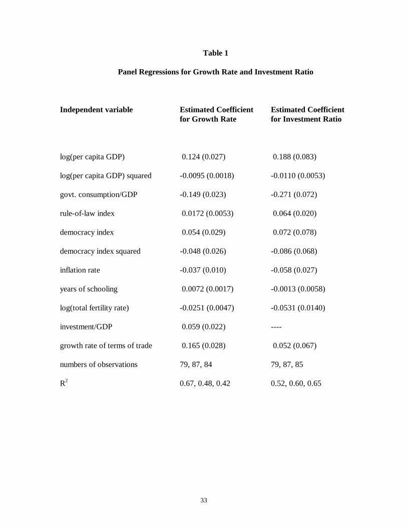
Table 1 shows panel regression estimates for the determination of the growth rate

of real per capita GDP and the ratio of real investment to real GDP.2 The effects of the

starting level of real per capita GDP show up in the estimated coefficients[RB1] on the level

and square of log(GDP). The other regressors include an array of policy variables—the

ratio of government consumption to GDP, a subjective index of the maintenance of the

rule of law, a subjective index for democracy (electoral rights), and the rate of inflation.

ratio of human to physical capital.2 The GDP figures in 1985 prices are the purchasing-power-parity adjusted chain-weighted values fromSummers and Heston, version 5.6. These data are available on the internet from the National Bureau ofEconomic Research. See Summers and Heston (1991) for a general description of their data. Realinvestment (private plus public) is from the same source.

7

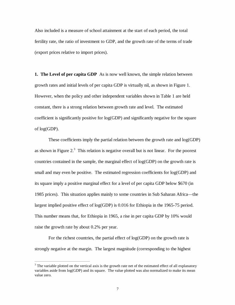
Also included is a measure of school attainment at the start of each period, the total

fertility rate, the ratio of investment to GDP, and the growth rate of the terms of trade

(export prices relative to import prices).

1. The Level of per capita GDP As is now well known, the simple relation between

growth rates and initial levels of per capita GDP is virtually nil, as shown in Figure 1.

However, when the policy and other independent variables shown in Table 1 are held

constant, there is a strong relation between growth rate and level. The estimated

coefficient is significantly positive for log(GDP) and significantly negative for the square

of log(GDP).

These coefficients imply the partial relation between the growth rate and log(GDP)

as shown in Figure 2.3 This relation is negative overall but is not linear. For the poorest

countries contained in the sample, the marginal effect of log(GDP) on the growth rate is

small and may even be positive. The estimated regression coefficients for log(GDP) and

its square imply a positive marginal effect for a level of per capita GDP below $670 (in

1985 prices). This situation applies mainly to some countries in Sub Saharan Africa—the

largest implied positive effect of log(GDP) is 0.016 for Ethiopia in the 1965-75 period.

This number means that, for Ethiopia in 1965, a rise in per capita GDP by 10% would

raise the growth rate by about 0.2% per year.

For the richest countries, the partial effect of log(GDP) on the growth rate is

strongly negative at the margin. The largest magnitude (corresponding to the highest

3 The variable plotted on the vertical axis is the growth rate net of the estimated effect of all explanatoryvariables aside from log(GDP) and its square. The value plotted was also normalized to make its meanvalue zero.

8

value of per capita GDP) is for Luxembourg in 1995—the GDP value of $19794 implies a

marginal effect of -0.064 on the growth rate. The United States in 1995 has the next

largest GDP value ($18951) and also has an estimated marginal effect on GDP of -0.064.

These values mean that an increase in per capita GDP by 10% implies a decrease in the

growth rate on impact by 0.6% per year. However, higher levels of GDP tend to be

associated with levels of other explanatory variables—such as more schooling, lower

fertility, and better maintenance of the rule of law—that have offsetting implications for

growth.

Overall, the cross-country evidence shows no pattern of absolute convergence—

whereby poor countries tend systematically to grow faster than rich ones—but does

provide strong evidence of conditional convergence. That is, except possibly at extremely

low levels of per capita product, a poorer country tends to grow faster for given values of

the policy and other explanatory variables. The pattern of absolute convergence does not

appear because poor countries tend systematically to have less favorable values of the

determining variables other than log(GDP).

In the panel for the investment ratio in Table 1, the pattern of estimated

coefficients on log(GDP) is also positive on the linear term and negative on the square.

These values imply a hump-shaped relation between the investment ratio and the starting

level of GDP—the relation is positive for per capita GDP below $5100 and then becomes

negative.

2. Government Consumption The ratio of government consumption to GDP is

intended to measure a set of public outlays that do not directly enhance an economy’s

9

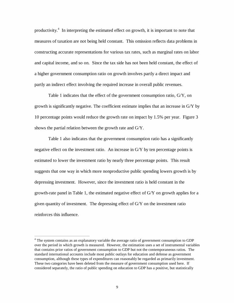
productivity.4 In interpreting the estimated effect on growth, it is important to note that

measures of taxation are not being held constant. This omission reflects data problems in

constructing accurate representations for various tax rates, such as marginal rates on labor

and capital income, and so on. Since the tax side has not been held constant, the effect of

a higher government consumption ratio on growth involves partly a direct impact and

partly an indirect effect involving the required increase in overall public revenues.

Table 1 indicates that the effect of the government consumption ratio, G/Y, on

growth is significantly negative. The coefficient estimate implies that an increase in G/Y by

10 percentage points would reduce the growth rate on impact by 1.5% per year. Figure 3

shows the partial relation between the growth rate and G/Y.

Table 1 also indicates that the government consumption ratio has a significantly

negative effect on the investment ratio. An increase in G/Y by ten percentage points is

estimated to lower the investment ratio by nearly three percentage points. This result

suggests that one way in which more nonproductive public spending lowers growth is by

depressing investment. However, since the investment ratio is held constant in the

growth-rate panel in Table 1, the estimated negative effect of G/Y on growth applies for a

given quantity of investment. The depressing effect of G/Y on the investment ratio

reinforces this influence.

4 The system contains as an explanatory variable the average ratio of government consumption to GDPover the period in which growth is measured. However, the estimation uses a set of instrumental variablesthat contains prior ratios of government consumption to GDP but not the contemporaneous ratios. Thestandard international accounts include most public outlays for education and defense as governmentconsumption, although these types of expenditures can reasonably be regarded as primarily investment.These two categories have been deleted from the measure of government consumption used here. Ifconsidered separately, the ratio of public spending on education to GDP has a positive, but statistically

10

3. The Rule of Law Many analysts believe that secure property rights and a strong legal

system are central for investment and other aspects of economic activity. The empirical

challenge has been to measure these concepts in a reliable way across countries and over

time. Probably the best indicators available come from international consulting firms that

advise clients on the attractiveness of countries as places for investments. These investors

are concerned about institutional matters such as the prevalence of law and order, the

capacity of the legal system to enforce contracts, the efficiency of the bureaucracy, the

likelihood of government expropriation, and the extent of official corruption. These kinds

of factors have been assessed by a number of consulting companies, including Political

Risk Services in its publication International Country Risk Guide.5 This source is

especially useful because it covers over 100 countries since the early 1980s. Although the

data are subjective, they have the virtue of being prepared contemporaneously by local

experts. Moreover, the willingness of customers to pay substantial fees for this

information is perhaps some testament to their validity.

Among the various indicators available, the index for overall maintenance of the

rule of law (also referred to as “law and order tradition”) turns out to have the most

explanatory power for economic growth and investment. This index was initially

measured by Political Risk Services in seven categories on a zero to six scale, with six the

most favorable. The index has been converted here to a zero-to-one scale, with zero

indicating the poorest maintenance of the rule of law and one the best.

insignificant, effect on economic growth. The ratio of defense outlays to GDP has roughly a zero relationwith economic growth.5 These data were introduced to economists by Knack and Keefer (1995). Two other consulting servicesthat construct these type of data are BERI (Business Environmental Risk Intelligence) and BusinessInternational (now a part of the Economist Intelligence Unit).

11

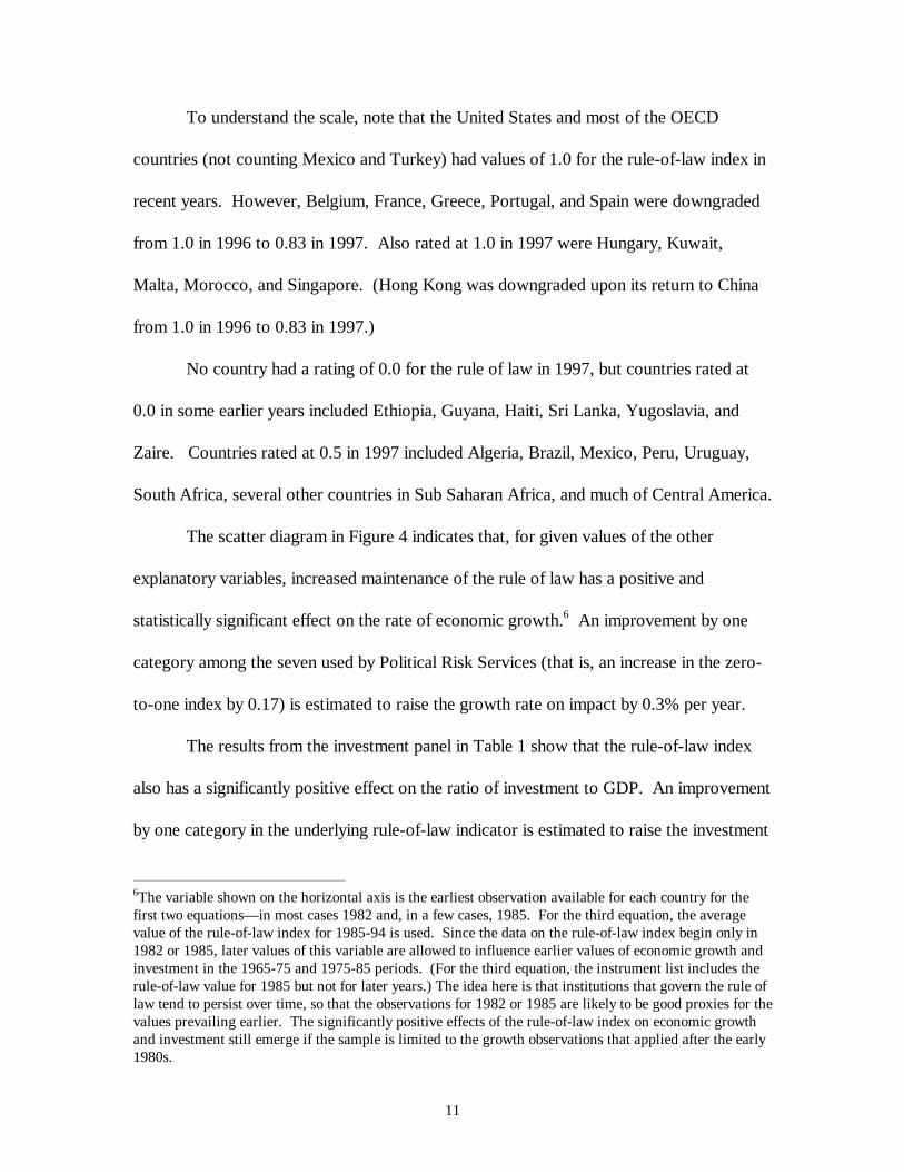
To understand the scale, note that the United States and most of the OECD

countries (not counting Mexico and Turkey) had values of 1.0 for the rule-of-law index in

recent years. However, Belgium, France, Greece, Portugal, and Spain were downgraded

from 1.0 in 1996 to 0.83 in 1997. Also rated at 1.0 in 1997 were Hungary, Kuwait,

Malta, Morocco, and Singapore. (Hong Kong was downgraded upon its return to China

from 1.0 in 1996 to 0.83 in 1997.)

No country had a rating of 0.0 for the rule of law in 1997, but countries rated at

0.0 in some earlier years included Ethiopia, Guyana, Haiti, Sri Lanka, Yugoslavia, and

Zaire. Countries rated at 0.5 in 1997 included Algeria, Brazil, Mexico, Peru, Uruguay,

South Africa, several other countries in Sub Saharan Africa, and much of Central America.

The scatter diagram in Figure 4 indicates that, for given values of the other

explanatory variables, increased maintenance of the rule of law has a positive and

statistically significant effect on the rate of economic growth.6 An improvement by one

category among the seven used by Political Risk Services (that is, an increase in the zero-

to-one index by 0.17) is estimated to raise the growth rate on impact by 0.3% per year.

The results from the investment panel in Table 1 show that the rule-of-law index

also has a significantly positive effect on the ratio of investment to GDP. An improvement

by one category in the underlying rule-of-law indicator is estimated to raise the investment

6The variable shown on the horizontal axis is the earliest observation available for each country for thefirst two equations—in most cases 1982 and, in a few cases, 1985. For the third equation, the averagevalue of the rule-of-law index for 1985-94 is used. Since the data on the rule-of-law index begin only in1982 or 1985, later values of this variable are allowed to influence earlier values of economic growth andinvestment in the 1965-75 and 1975-85 periods. (For the third equation, the instrument list includes therule-of-law value for 1985 but not for later years.) The idea here is that institutions that govern the rule oflaw tend to persist over time, so that the observations for 1982 or 1985 are likely to be good proxies for thevalues prevailing earlier. The significantly positive effects of the rule-of-law index on economic growthand investment still emerge if the sample is limited to the growth observations that applied after the early1980s.

12

ratio by about 1.1 percentage points. The stimulus to investment is one way that better

maintenance of the rule of law would encourage growth. However, since the investment

ratio is held constant in the growth panel in Table 1, the estimated positive effect of the

rule-of-law indicator on growth applies for a given quantity of investment. The

stimulative effect on the investment ratio reinforces this influence.

4. Democracy Another strand of research on the role of institutions has focused on

democracy, specifically on the strength of electoral rights and civil liberties. In this case,

the theoretical effects on investment and growth are ambiguous. One effect, characteristic

of systems of one-person/one-vote majority voting, involves the pressure to enact

redistributions of income from rich to poor. These redistributions may involve land

reforms and social-welfare programs. Although the direct effects on income distribution

may be desirable (because they are equalizing), these programs tend to compromise

property rights and reduce the incentives of people to work and invest. One kind of

disincentive involves the transfers given to poor people. Since the amount received

typically falls as the person earns more income, the recipient is motivated to remain on

welfare or otherwise disengage from productive activity. The other adverse effect

involves the income taxes or other levies that are needed to pay for the transfers. An

increase in these taxes encourages the non-poor to work and invest less.

One offsetting effect is that an evening of income distribution may reduce the

tendency for social unrest. Specifically, transfers to the poor may reduce incentives to

13

engage in criminal activity, including riots and revolutions.7 Since social unrest reduces

incentives to work and invest, some amount of publicly organized income redistribution

may contribute to overall economic activity. However, even a dictator would be willing to

engage in transfers to the extent that the decrease in social unrest was worth the cost of

the transfers. Thus, the main point is that democracy will tend to generate “excessive”

transfers purely from the standpoint of maximizing the economy’s total output.

Although democracy has its down side, one cannot conclude that autocracy

provides ideal economic incentives. One problem with dictators is that they have the

power and, hence, the inclination to steal the nation’s wealth. More specifically, an

autocrat may find it difficult to convince people that their property will not be confiscated

once investments have been made. This convincing can sometimes be accomplished

through reputation—that is, from a history of good behavior—but also by relaxing to

some degree the hold on power. In this respect, an expansion of democracy—viewed as a

mechanism for checking the power of the central authority—may enhance property rights

and, thereby, encourage economic activity. From this perspective, democracy would

encompass not only electoral rights but also civil liberties that allow for freedom of

expression, assembly, and so on.

A number of researchers have provided quantitative measures of democracy, and

Alex Inkeles (1991, p. x) finds in an overview study a “high degree of agreement produced

by the classification of nations as democratic or not, even when democracy is measured in

somewhat different ways by different analysts.” One of the most useful measures—

7 Data are available across countries on numbers of revolutions, riots, and so on. However, once the rule-of-law index is held constant, these measures of social unrest turn out to lack significant explanatorypower for growth and investment.

14

because it is available for almost all countries annually on a consistent basis since 1972—is

the one provided by Gastil (1982-83 and other years) and his followers at Freedom House.

This source provides separate indexes for electoral rights and civil liberties.

The Freedom House concept of electoral rights uses the following basic definition:

“Political rights are rights to participate meaningfully in the political process. In a

democracy this means the right of all adults to vote and compete for public office, and for

elected representatives to have a decisive vote on public policies” (Gastil, 1986-87 edition,

p. 7). In addition to the basic definition, the classification scheme rates countries

(somewhat impressionistically) as less democratic if minority parties have little influence

on policy.

Freedom House applies the concept of electoral rights on a subjective basis to

classify countries annually into seven categories, where group one is the highest level of

rights and group seven is the lowest. This classification was made by Gastil and his

associates and followers based on an array of published and unpublished information about

each country. The original ranking from one to seven was converted here to a scale from

zero to one, where zero corresponds to the fewest rights (Freedom House rank seven) and

one to the most rights (Freedom House rank one). The scale from zero to one

corresponds to a classification made by Kenneth Bollen (1990) for 1960 and 1965. The

Bollen index differs mainly in that its concept of democracy goes beyond electoral rights.

To fix ideas on the meaning of the zero-to-one subjective scale, note first that the

United States and most other OECD countries in recent years received the value 1.0,

thereby being designated as full representative democracies. Dictatorships that received

the value 0.0 in 1996 included China, Indonesia, Iraq, Saudi Arabia, Syria, and several

15

countries in sub Saharan Africa. Places that were rated in 1996 at 0.5—halfway along

between dictatorship and democracy—included Colombia, Ethiopia, Haiti, Jordan,

Malaysia, Mexico, Nicaragua, Pakistan, Paraguay, Peru, Senegal, Singapore, Turkey, and

Uganda.

The Freedom House index of civil liberties is constructed in a similar way. The

definition here is “civil liberties are rights to free expression, to organize or demonstrate,

as well as rights to a degree of autonomy such as is provided by freedom of religion,

education, travel, and other personal rights” (Gastil, 1986-87 edition, p. 7). In practice,

the indicator for civil liberties is extremely highly correlated with that for electoral rights.

Thus, for practical purposes, it makes little difference in the analysis of growth and

investment whether one uses the index for electoral rights or the one for civil liberties.

The empirical work discussed here uses the index of electoral rights and sometimes refer

to this indicator as simply a measure of democracy.

With the other independent variables shown in Table 1 held constant, the overall

relation between the growth rate and the democracy index turns out to be close to zero.

The results shown in the table suggest a non-linear relationship—positive on the level of

democracy and negative on the square of democracy. However, since a Wald test for the

joint significance of the two democracy variables has a p-value of 0.18, the statistical

support for this relationship is weak.

The fitted relation between growth and democracy is shown in Figure 5. As the

Wald test suggested, the overall relation between growth and democracy is weak. In

particular, there are examples of dictatorships (values of electoral rights near zero) with

high and low rates of growth and similarly for democracies (values of democracy near

16

one). Analogous findings apply to the effect of democracy on the investment ratio, as

shown in Table 1.

The results should not be taken as saying that dictatorship is desirable from the

standpoint of economic performance. There are examples of autocrats—such as Pinochet

in Chile, Fujimori in Peru, the Shah in Iran, and Lee and several others in East Asia—that

produced good growth outcomes. There are, however, other examples—including

Marcos in the Philippines, Mao in China, Mobutu and numerous other despots in Africa,

and many others in South America and eastern Europe—that delivered poor growth

outcomes. However, the findings also do not support the oft-mentioned idea that

democracy is necessary for growth.

5. The Inflation Rate Table 1 shows a significantly negative effect of inflation (based on

consumer price indexes) on the rate of economic growth.8 The estimated coefficient

implies that an increase in the average rate of inflation by 10 % per year would lower the

growth rate on impact by 0.4% per year.

Figure 6 shows the partial relation between growth and inflation. In the upper

panel, which includes the full range of inflation, the estimated effect of inflation is

significantly negative. However, the relation appears to be driven by the observations of

8 Because of the concern about reverse causation—lower growth causing higher inflation—the panelestimation in Table 1 does not contain contemporaneous or lagged values of inflation or money growth inthe set of instruments. Rather, the system includes dummy variables for prior colonial history asinstruments. These dummy variables have substantial predictive content for inflation. (An attempt to usecentral-bank independence as an instrument failed because this variable turned out to lack predictivecontent for inflation.) The estimated coefficient on the inflation rate has a smaller magnitude but is stillsignificantly negative if lagged inflation is included with the instruments.

17

extreme inflation. (Note that 1.0 on the horizontal axis signifies inflation at the

continuously compounded rate of 100% per year.)

The middle panel of Figure 6 shows that the relation between growth and inflation

is only weakly negative (and not statistically significant) if one considers only moderate

inflation, up to rates of 20% per year. The bottom panel shows that a clear negative

relationship applies for higher rates of inflation. Despite these apparent differences in the

effects of inflation at low and high levels, a Wald test accepts the hypothesis that the effect

of inflation on growth in the low range of inflation (middle panel) is the same as that in

the high range (bottom panel). In any event, there is no indication in the data over any

range of a positive effect of inflation on growth. That is, for growth averaged over ten

years, there is no sign that an economy has to accept more inflation to achieve better real

outcomes.

Table 1 shows that inflation also has a negative effect on the investment ratio.

This depressing effect on investment would reinforce the direct negative effect on growth

that has already been discussed.

6. Education Governments typically have strong direct involvement in the financing and

provision of schooling at various levels. Hence, public policies in these areas have major

effects on a country’s accumulation of human capital. One measure of this schooling

capital is the average years of attainment, as constructed by Barro and Lee (1997). These

data are classified by sex and age (for persons aged 15 and over and 25 and over) and by

levels of education (no school, partial and complete primary, partial and complete

secondary, and partial and complete higher).

18

In growth-accounting exercises, the growth rate would be related to the change in

human capital—say the change in years of schooling—over the sample period. My

approach, however, is to think of changes in capital inputs, including human capital, as

jointly determined with economic growth. These variables all depend on (hopefully

exogenous) policy variables and national characteristics and on initial values of state

variables, including stocks of human and physical capital.

For a given level of initial per capita GDP, a higher initial stock of human capital

signifies a higher ratio of human to physical capital. This higher ratio tends to generate

higher economic growth through at least two channels. First, more human capital

facilitates the absorption of superior technologies from leading countries. This channel is

likely to be especially important for schooling at the secondary and higher levels. Second,

human capital tends to be more difficult to adjust than physical capital. Therefore, a

country that starts with a high ratio of human to physical capital—such as in the aftermath

of a war that destroys primarily physical capital—tends to grow rapidly by adjusting

upward the quantity of physical capital.

Table 1 shows that the average years of school attainment at the secondary and

higher levels for males aged 25 and over has a positive and significant effect on the

subsequent rate of economic growth.9 The estimated coefficient implies than an additional

year of schooling raises the growth rate on impact by 0.7% per year. As already

mentioned, one interpretation of this effect is that a work force educated at the secondary

and higher levels facilitates the absorption of technologies from more advanced foreign

countries.

9 The results are basically the same if the years of attainment apply to persons aged 15 and over.

19

Female schooling at the secondary and higher levels turns out not to have

significant explanatory power for growth—if this variable is added to the growth panel, its

estimated coefficient is -0.0044 (s.e.=0.0040). Note, however, that female education has a

strong negative effect on fertility rates, and the fertility variable is already held constant in

the growth panel. If fertility is not held constant, then female schooling appears somewhat

more important for growth (with a coefficient that is roughly zero, rather than negative).

One possible explanation for the weak role of female schooling in the growth panel is that

many countries follow discriminatory practices that prevent the efficient exploitation of

females in the formal labor market. Given these practices, it is not surprising that more

resources devoted to female education would not show up as enhanced growth.

Years of attainment of males or females at the primary level turn out to be

insignificant for growth. The special importance of schooling at the secondary and higher

levels supports the idea that education affects growth particularly by facilitating the

absorption of new technologies—which are likely to be complementary with labor

educated to these higher levels. Primary schooling is, however, critical as a prerequisite

for secondary schooling.

Table 1 indicates that years of schooling (for males at the secondary and higher

levels) are insignificantly related to the investment ratio. Hence, the linkage between

human capital and growth does not involve an expansion in the intensity of physical

capital. This result is inconsistent with the effects mentioned before involving the ratio of

human to physical capital.

Many researchers argue that the quality of schooling is more important than the

quantity, measured, for example, by years of attainment. Barro and Lee (1997) discuss the

20

available cross-country aggregate measures of the quality of education. Hanushek and

Kim (1995) find that scores on international examinations—an indicator of the quality of

schooling capital—matters more than years of attainment for subsequent economic

growth. My preliminary results support this finding.

Information on test scores—for science, reading, and mathematics—are available

for 51 of the countries in my sample. One drawback of these data, however, is that the

observations apply to different years and are most plentiful in the 1990s. In any event, the

available data were used to construct a single cross section of test scores for the 51

countries. If this variable is added to the panel system for growth, then the estimated

coefficient on the test-score variable is highly significant—0.101 (s.e.=0.027).10 The male

secondary and higher schooling variable remains significant but the estimated coefficient

falls by about one-half from the value shown in Table 1—the estimate is now 0.0035

(s.e.=0.0015). Hence, there is a suggestion that the quality and quantity of schooling both

matter for growth.

The results just described result if the cross-sectional test-score variable is included

in the instrument list for each time period. One problem with this procedure is that later

values of test scores are allowed, in some cases, to influence prior values of growth rates.

However, the results are nearly the same if the instrument list omits the test-score variable

and includes instead only prior values of variables that have predictive content for test

scores. These variables are the total years of schooling of the adult population (a proxy

for the education of parents) and pupil-teacher ratios at the primary and secondary levels.

10 This system has 40 observations for 1965-75, 43 for 1975-85, and 43 for 1985-95. There is someindication that science test scores have the most explanatory power for growth, although it is difficult to

21

Results are also similar if prior values of school dropout rates—which are inversely related

to test scores—are added as instruments.

7. Fertility Rate Table 1 shows that economic growth is significantly negatively related

to the total fertility rate. Thus, the choice to have more children per adult—and, hence, in

the long run to have a higher rate of population growth—comes at the expense of growth

in output per person. It should be emphasized that this relation applies when variables

such as per capita GDP and education are held constant. These variables are themselves

substantially negatively related to the fertility rate. Thus, the estimated coefficient on the

fertility variable likely isolates differing underlying preferences across countries on family

size, rather than effects related to the level of economic development. The partial relation

between the growth rate and the fertility rate is shown in Figure 8.

Table 1 also reveals a significant negative relation between the investment ratio

and the fertility rate. This relation can be interpreted as an indication that numbers of

children is a form of saving that is a substitute for other types of saving (which support

physical investment). The negative effect of the fertility rate on the investment ratio

reinforces the direct inverse effect of fertility on growth.

8. Investment Ratio Table 1 shows that the growth rate depends positively on the

investment ratio. This effect applies for given values of policy and other variables, as

already discussed, which affect the investment ratio. For example, an improvement in the

rule of law raises investment and also raises growth for a given amount of investment.

separate this variable statistically from mathematics scores. For given science scores, reading scores have

22

Thus, the estimated coefficient of the investment ratio in the growth panel—0.059

(s.e.=0.022)—is interpretable as an effect from a greater propensity to invest for given

values of the policy and other variables. For example, the effect would relate to the

investment ratio being higher because of a greater propensity to save (which would affect

domestic investment to the extent that an economy is not fully open) or because of some

unmeasured policies that influence investment. Recall also that the instrument list for the

estimation includes earlier values of the investment ratio but not values that are

contemporaneous with the growth rate. Hence, there is some reason to believe that the

estimated relation reflects effects of greater investment on the growth rate, rather than a

reverse effect from higher growth (and the accompanying better investment opportunities)

on the investment ratio.

Figure 9 shows the partial relation between the growth rate and the investment

ratio. The implied effect—with an estimated coefficient of 0.059 in Table 1—suggests that

an economy’s real rate of return to investment is reasonable but not astronomical.

9. The Terms of Trade Table 1 indicates that improvements in the terms of trade (a

higher growth rate of the ratio of export prices to import prices) enhance economic

growth but are insignificantly related to the investment ratio. The measurement of growth

rates in terms of changes in real GDP means that this relation is not a mechanical one.

That is, if patterns of employment and production are unchanged, then an improvement in

the terms of trade would raise real income and probably real consumption but would have

roughly a zero relation with economic growth.

23

a zero effect on real GDP. The positive impact of an improvement in the terms of trade

on real GDP therefore reflects increases in factor employments or productivity.

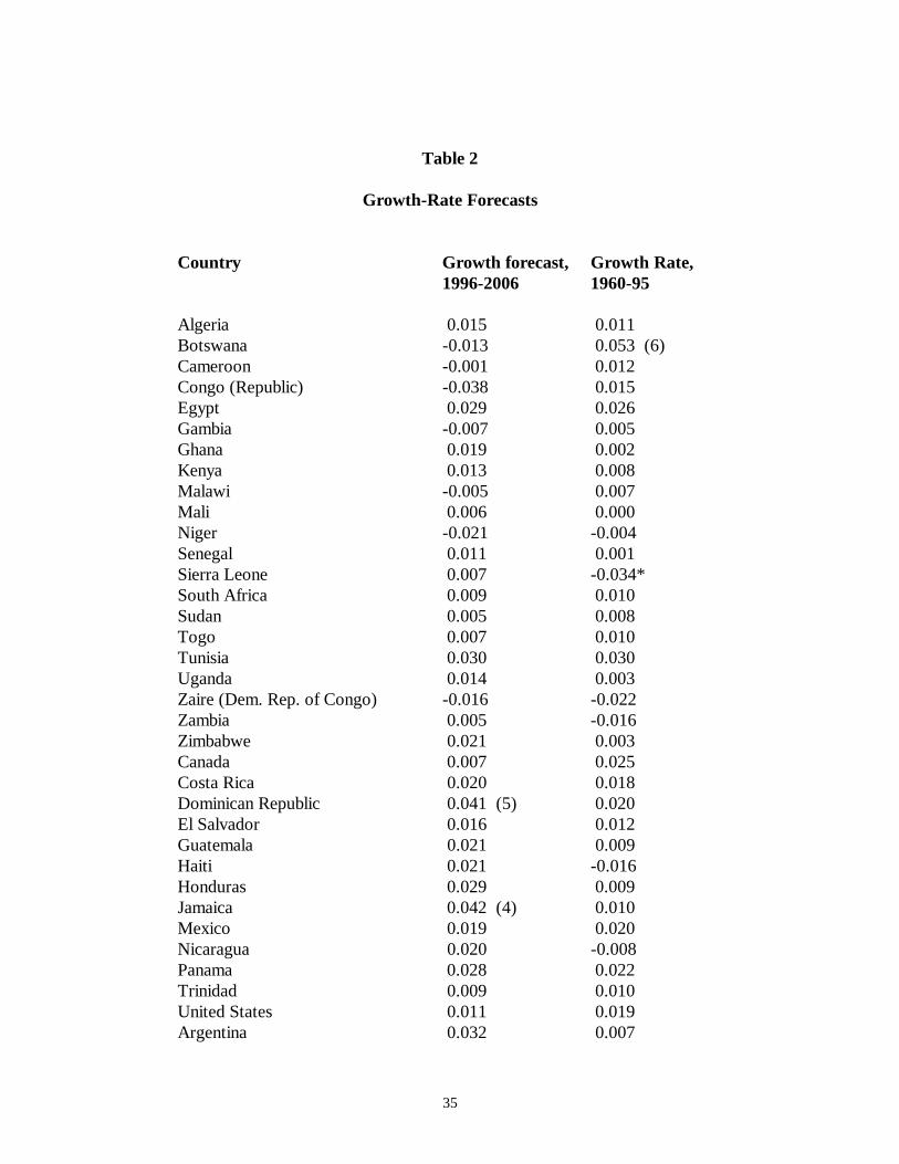
C. Growth-Rate Forecasts

The system estimated over the period 1965-95 can be adapted to generate growth

forecasts for the period after 1995. These forecasts are based on the latest available

observations on the variables that have already been discussed. For most countries and

variables, the data are for 1996. However, the figures on schooling, government

consumption, and investment are for the early 1990s. In most cases—aside from the

growth rate of the terms of trade—the historical relationships indicate that these latest

observations on the explanatory variables would have substantial predictive power for the

sample averages of these variables over the forecast period, 1996-2006.

The growth-rate panel discussed in Table 1 was reestimated (by the seemingly-

unrelated method) using only prior values of the regressors. For example, for 1965-75,

this system has as explanatory variables log(GDP) and its square for 1965, the government

consumption ratio for 1960-64, the earliest available value for the rule-of-law variable (for

1982 or 1985), democracy and its square in 1965, inflation for 1960-65, schooling in

1965, fertility in 1965, and the investment ratio for 1960-64. The predicted values of the

per capita growth rate for 1996-2006 generated from this system are shown for the 88

countries with the necessary data in Table 2.11 The actual growth rates from 1960 to 1995

are also shown in the table.

11 The constant term used here is the one that applies to the 1985-95 period. For China, Hungary, andPoland, rough estimates were used for the government consumption ratio.

24

For all 110 countries with the data on GDP, the average growth rate of per capita

GDP from 1960 to 1995 was 1.8% per year. Some regional average growth rates were

4.3% for 11 east Asian countries, 2.6% for 24 OECD countries, 1.2% for 24 Latin

American countries, and 0.7% for 37 sub Saharan African countries.

The group of high-growing countries was, as is well known, dominated by East

Asian countries—South Korea first at 6.6%, Taiwan second at 6.1%, Hong Kong third at

5.9%, Singapore fourth at 5.6%, Thailand seventh at 4.8%, Japan eighth at 4.7%, and

Malaysia ninth at 4.5%. The other countries in the top-ten list were Malta (fifth at 5.3%),

Botswana (sixth at 5.3%), and Cyprus (tenth at 4.4%).

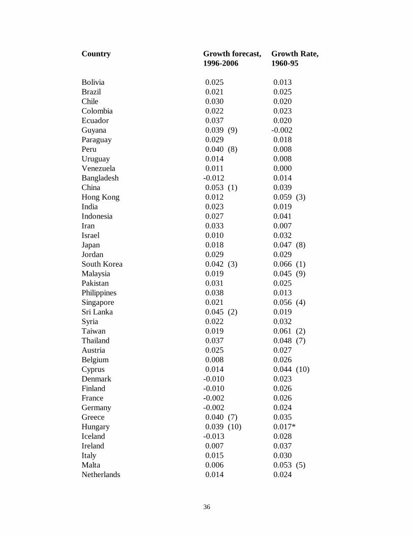
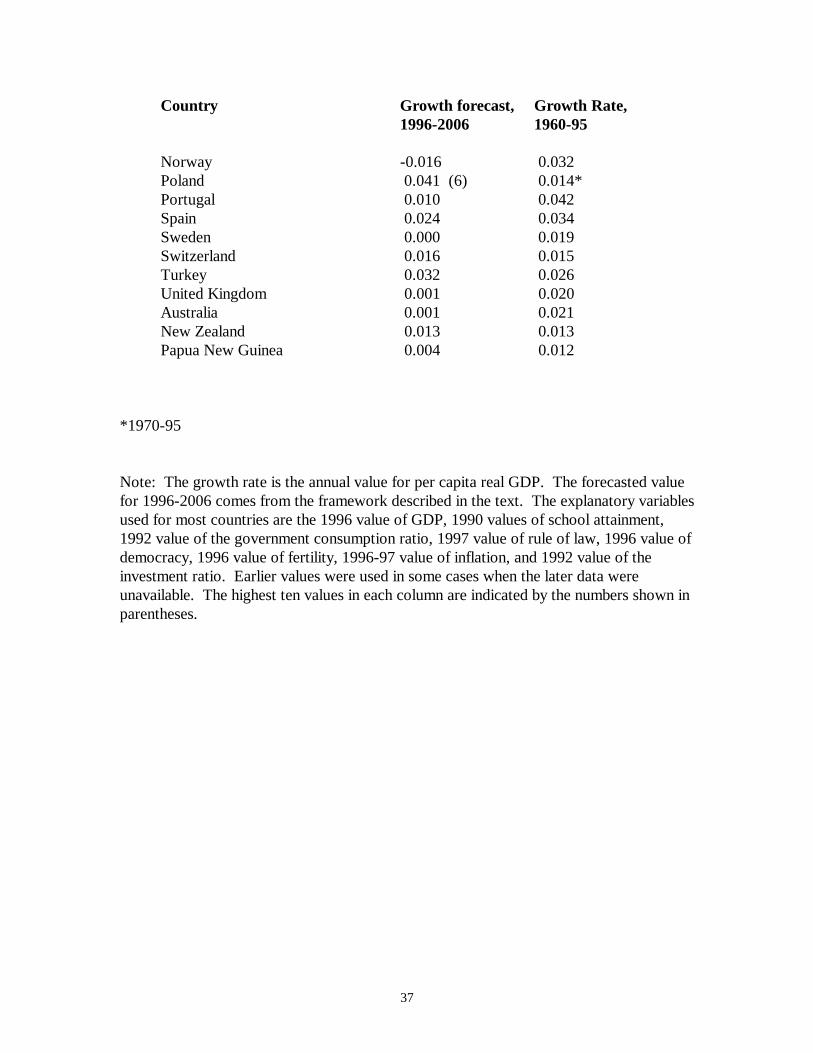
For the forecasts of growth from 1996 to 2006, the average value for 88 countries

with the necessary data is 1.6% per year.12 Regional averages are 2.7% for 11 east Asian

countries, 0.8% for 23 OECD countries, 2.6% for 22 Latin American countries, and 0.1%

for 18 sub Saharan African countries. The reduction in projected performance for the east

Asian and OECD countries—compared with actual growth rates from 1960 to 1995—

reflects especially the workings of the convergence force. These places are now pretty

rich on average, even in comparison with years of schooling and the values of the other

independent variables. The projected increase of growth in Latin America reflects

particularly improvements in policy variables, including reduced inflation and better

maintenance of the rule of law.

In the list of projected high growers, east Asian countries are much less prominent

than before—the only ones appearing on the top-ten list are China (first at 5.3%) and

South Korea (third at 4.2%). The transition economies of Poland (sixth at 4.1%) and

12 Note that the constant term is, by assumption, the one applying for the 1985-95 period.

25

Hungary (tenth at 3.9%) are on the list, and other formerly non-market economies would

likely be present if the data were available. The other high-growth forecasts are mixed

geographically, including Sri Lanka, Trinidad, Dominican Republic, Greece (the only

OECD representative), Peru, and Guyana.

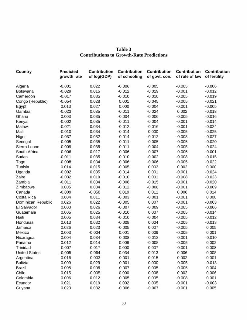
One way to understand the pattern of forecasts is to break down the growth

prediction (expressed as a deviation from the sample mean) into contributions from each

of the explanatory variables. These variables, each expressed as deviations from their

respective sample means, are log(GDP) and its square, the government consumption ratio,

the rule of law, democracy and its square, the inflation rate, years of schooling, the fertility

rate, and the investment ratio. For instance, a relatively high value of log(GDP)

contributes a negative amount to the growth prediction. This effect is the conditional-

convergence force. Relatively good values of policy variables—low government

consumption, high rule of law, and low inflation—contribute positively to the growth

forecast. Similarly, the growth contribution is positive for high years of schooling, low

fertility, and high investment. The democracy variable has a nonlinear effect, but the

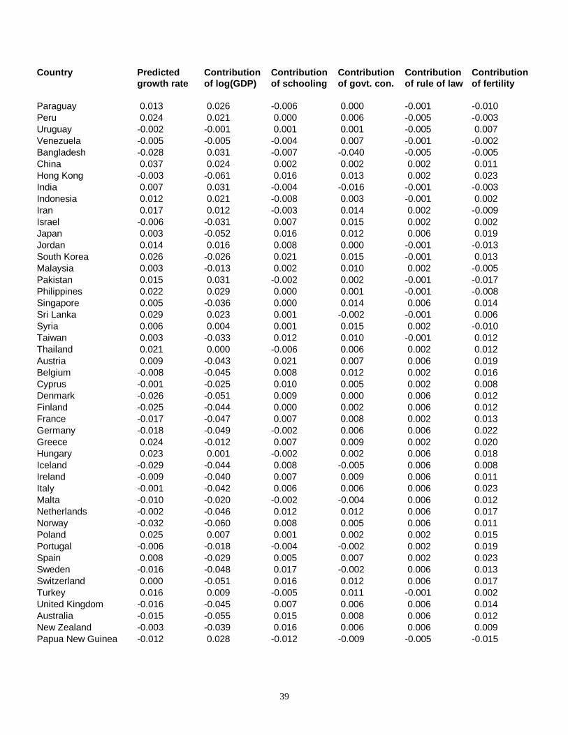
overall magnitudes here are small. Table 3 shows the values of the contributions for the

explanatory variables that turned out to be most important—log(GDP) and its square,

schooling, government consumption, the rule of law, and the fertility rate.

As an example, for the United States, the extremely high value of log(GDP)

contributes -0.064 to the growth forecast because of the large convergence effect. This

negative contribution is, however, offset by positive effects from high years of schooling

(0.034), low government consumption (0.013), strong rule of law (0.006), and low

fertility (0.008). Therefore, the U.S. per capita growth-rate forecast of 0.011 is only

26

0.005 below the sample mean of 0.016. For some other OECD countries—Denmark,

Finland, France, Germany, Iceland, Norway, and Sweden—the offset to the negative

convergence force is not as great and the forecasted per capita growth rates are zero or

negative. For a transition economy such as China, the contribution from log(GDP) is

positive (0.024), and the reasonably good values of the other explanatory variables

reinforce this effect.

One way to assess the likely reliability of the growth projections is to use the data

up to 1985 to make “forecasts” for 1985-95. These within-sample projections can be

compared with observed growth rates for this ten-year period. To carry out this

procedure, the growth-rate panel was reestimated over the two periods 1965-75 and

1975-85—that is, the period 1985-95 was excluded from this system. As with the

projections discussed before, the equations included only prior values of the regressors.

The resulting coefficient estimates (from the seemingly-unrelated technique) turn out to be

basically similar to those generated from the three-period panel.13

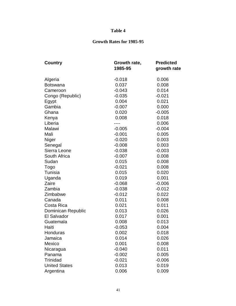
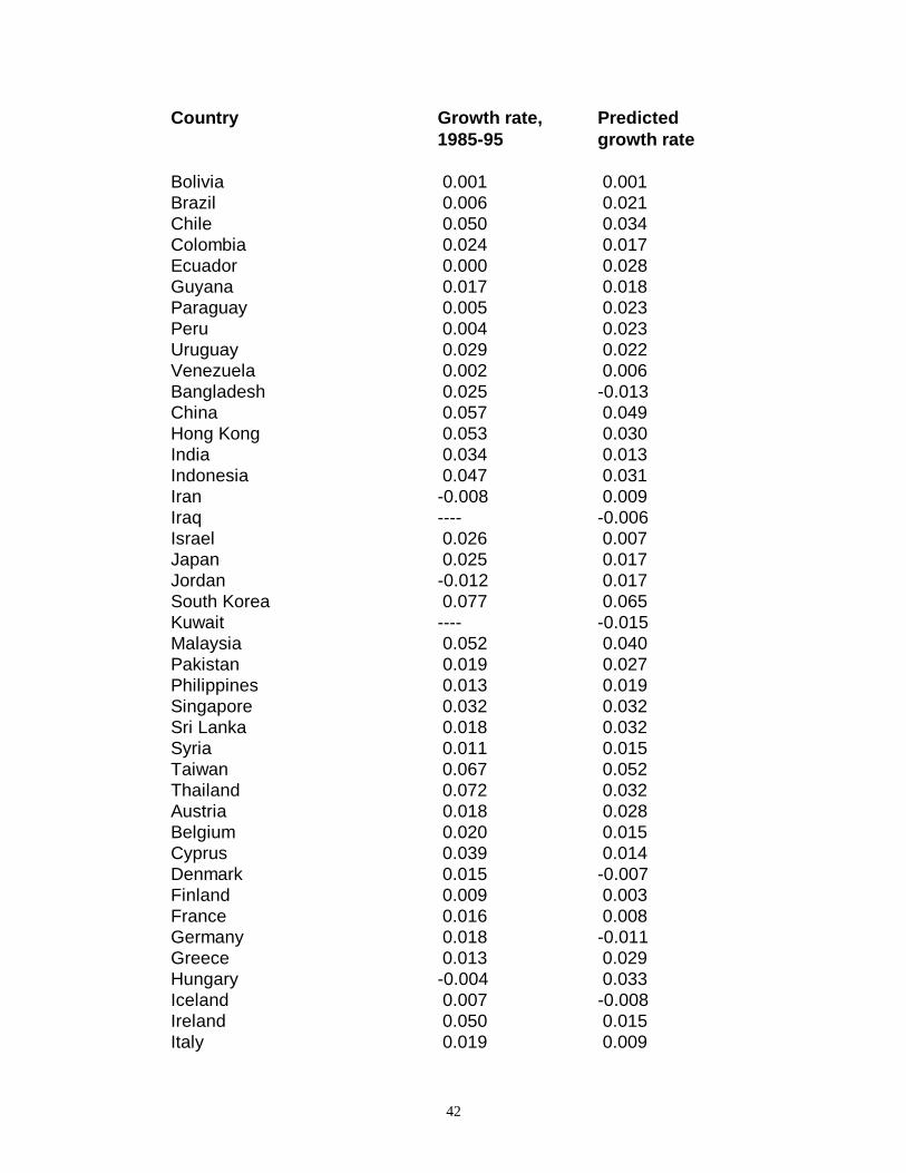
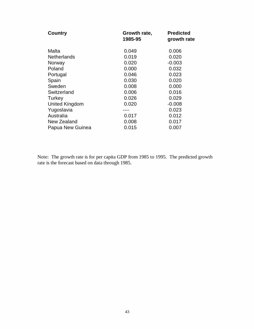
Table 4 shows the resulting projections of growth rates for 1985-95 along with the

actual values. For the 88 countries that have data on projected and actual values, the

correlation is 0.56, corresponding to a prediction R2 of 0.31. In contrast, the R2 value for

the 1985-95 period is 0.46 in the three-period estimation based only on lagged variables.14

This better fit emerges because the observations for 1985-95 were allowed to influence the

13 However, a Wald test of equality for the coefficients of all ten explanatory variables (not including theconstant term) for the first two periods versus the third period has a p-value for rejection of only 0.003.14 The fit would also be expected to improve with knowledge of the contemporaneous values of theregressors, rather than just the lagged values. However, the R2 value for 1985-95 in the system in Table 1that includes contemporaneous values of the independent variables is only 0.42. This result is notprecisely comparable to those from the systems with lagged variables, which were estimated by theseemingly-unrelated technique, because the system in Table 1 was estimated by instrumental variables. If

27

estimation of the coefficients in the three-period setting. In any event, the conclusion is

that the empirical growth framework has substantial predictive content for growth rates

but that substantial prediction errors remain.

D. Other Policy Influences on Growth and Investment

1. Public Debt The results described thus far for traditional fiscal and monetary policy

involve government consumption and inflation. The choice of public financing between

current and future taxation—or, equivalently, between taxes and public borrowing—is

often thought also to matter for economic growth. In a closed economy, the predicted

effect is that more public debt would depress national saving and lead thereby to lower

growth. This effect would arise for past budget deficits, as reflected in current debt levels,

and also for prospective future borrowing. In an open economy, the predicted effects of

public debt on domestic investment and growth are mitigated by foreign borrowing but

still apply to the extent that international capital markets are “imperfect” or that the home

economy is large enough to matter for world aggregates.

To assess the effects of public debt on economic growth and investment, I use a

recently constructed data set on ratios of consolidated central government debt to GDP.

The underlying data come from IMF publications and other country sources. The figures

refer to five-year averages over the period 1960 to 1994 and are available for a subset of

the observations considered before.

this system is estimated by the seemingly-unrelated method, then the R2 value for the third period is 0.46.If the system is fit by ordinary least squares, then the value is 0.49.

28

If the debt-GDP ratio is added to the system described in Table 1, then the

estimated coefficient of this new variable is -0.0045 (s.e.=0.0034).15 Hence, the effect is

negative but not statistically significant. Recall, however, that this system holds constant

the investment ratio, and the usual view is that more public debt depresses growth by

lowering investment. In the system for the investment ratio, the estimated coefficient of

the debt-GDP ratio is 0.0077 (s.e.=0.0100). Hence, there is no indication that more public

debt depresses investment.

From the standpoint of a supporter of Ricardian equivalence—whereby the choice

between taxes and public debt does not matter for much—these cross-country results have

to be gratifying. On the other hand, after so much effort was expended in the construction

of this new data set on government debt, it would have been nice to obtain stronger

findings. At this point, the conclusion seems to be that ratios of public debt to GDP

matter little for an economy’s subsequent rates of economic growth and investment.

2. Labor-Market Restrictions Labor-market restrictions imposed by governments are

often thought to underlie the sluggish recent performance of many countries in western

Europe. The public interventions include mandated levels of wages and benefits,

restrictions on labor turnover, and encouragement of collective bargaining. The

assessment of the effects of these kinds of policies for a broad sample of countries has

been hindered by lack of good data. To get a rough idea of whether these sorts of

15 The system includes the average ratio of debt to GDP over each period. The instrument lists include theaverage debt-GDP ratio over the five-year earlier period. For example, the 1965-75 growth-rate equationincludes as an independent variable the average of the debt-GDP ratio from 1965 to 1975 and includes asan instrument the average of this ratio from 1960 to 1964.

29

restrictions matter a lot for growth, I used a rough proxy for the extent of these

restrictions.

The approach is based on the labor-standards conventions adopted by the

International Labor Organization (ILO).16 Once ratified by an individual member state

(which includes most countries other than Taiwan and Hong Kong), a labor standard is

supposed to be binding in terms of international law. Since its inception in 1919, the ILO

conference has adopted 174 conventions.17 Many of these provisions are not very

controversial, covering matters such as elimination of forced labor, freedom of

association, and discrimination. Others are more directly related to the kinds of labor-

market interventions that would hinder economic performance.

For present purposes, I consider country ratifications of four of the ILO

conventions that seem to relate closely to intervention into labor markets: minimum-wage

fixing (no. 131, adopted in 1970), restrictions on termination of employment (no. 158,

1982), promotion of collective bargaining (no. 154, 1981), and equal pay for men and

women (no. 100, 1951). At one extreme, all four of these provisions had been ratified by

1994 by Spain, Niger, and Zambia, whereas none had been ratified by the United States,

Botswana, Mauritius, South Africa, South Korea, Malaysia, Singapore, Thailand, and a

few other places.

Although the adoption of an ILO convention likely would not matter much directly

for a country’s labor-market policy, the number of these ratifications may nevertheless

proxy for the government’s general stance with regard to intervention into labor markets.

16 These measures have been employed previously by Rodrik (1996).17 For descriptions of the main conventions, see International Labour Organization (1990). Information oncountry ratifications is contained in International Labour Organization (1995).

30

If the number of ratifications (at any date up to 1994) of the four conventions is added to

the system in Table 1, then the estimated coefficient of the ILO variable is -0.0059

(s.e.=0.0043) in the growth-rate system and 0.031 (s.e.=0.019) in the investment-ratio

system.18 The point estimates suggest that more regulation lowers growth for given

investment but tends to raise investment. Since neither coefficient estimate is statistically

significant, the best inference is probably that the ILO number is not a good proxy for the

state of labor-market regulation. Hence, cross-country estimation of the effects of labor-

market regulation requires better data on these regulations.

3. Other Policy Influences on Growth and Investment Other researchers have studied

additional ways in which government policies affect economic growth. Sachs and Warner

(1995) focus on international openness, as reflected in tariff and non-tariff barriers, the

black-market premium on foreign exchange, and subjective measures of open policies.

The overall finding is that increased openness to international trade promotes economic

growth. In my own research, I have found, however, that it is difficult to isolate these

effects once the variables described earlier in this paper are held constant. My view is that

this difficulty reflects problems in measuring policies that influence international openness,

not the lack of importance of this openness.

King and Levine (1993) analyzed the development of domestic capital markets.

They used various proxies for this development, including the extent of intermediation by

commercial banks and other domestic financial institutions. The general finding is that the

presence of a more advanced domestic financial sector predicts higher economic growth.

18 These systems include the one ILO variable in all three equations and all three instrument lists.

31

The main outstanding issue here is to disentangle the effect of financial development on

growth from the reverse channel. In particular, it is important for future research to

isolate the effects of government policies—for example, on regulation of domestic capital

markets—on the state of financial development and, hence, on the rate of economic

growth.

Easterly and Levine (1993) examined aspects of public investment and also

considered the nature of tax systems. One result is that public investment does not exhibit

high rates of return overall. The main positive effects on economic growth showed up for

investments in the area of transportation. With regard to tax systems, the findings were

largely inconclusive because of the difficulties in measuring marginal tax rates on labor and

capital incomes in a consistent and accurate way for a large sample of countries. An

important priority for future research is better measurement of the nature of tax systems.

III. Implications of the Cross-Country Findings for the Most Advanced Countries

The cross-country evidence provides good and bad news for the growth prospects

of the United States and other advanced countries. The good news is that the basic

institutions and policies of these successful places are favorable in comparison with those

of most other countries. In particular, the legal systems and public bureaucracies function

reasonably well, markets and price systems are allowed to operate to a considerable

extent, and high inflation is unusual. The population is also highly educated and rich.

The bad news is that successful countries cannot grow rapidly by filling the

vacuum of non-working public institutions or by absorbing the technologies and ideas that

have been developed elsewhere. Moreover, the levels of physical and human capital are

32

already high, and further accumulations are subject to diminishing returns. (Although test

scores—and, hence, schooling quality—could no doubt be improved substantially in the

United States.) These considerations result in the relatively low growth forecasts for the

most advanced countries in 1996-2006 that are shown in Tables 2 and 3—1.1% for the

United States, -0.2% for France and Germany, 0.1% for the United Kingdom, 0.7% for

Canada, and 0.0% for Sweden. Italy and Switzerland do somewhat better at 1.5% and

1.6%, respectively, and Japan is at 1.8% (well above its recent actual performance).

Sustained growth in the leading countries depends on innovations that lead to

new products and better methods of production, the factors stressed in the endogenous-

growth theories. This kind of technological progress occurs, and the rate of progress is

responsive to policies that shape the economic environment. However, the empirical

evidence suggests that feasible policies will not improve technology rapidly enough to

raise the long-term per capita growth rate above the range of 1- 2% per year. In fact,

maintaining this rate of advance will be a challenge in the long run.

33

Table 1

Panel Regressions for Growth Rate and Investment Ratio

Independent variable Estimated Coefficientfor Growth Rate

Estimated Coefficientfor Investment Ratio

log(per capita GDP) 0.124 (0.027) 0.188 (0.083)

log(per capita GDP) squared -0.0095 (0.0018) -0.0110 (0.0053)

govt. consumption/GDP -0.149 (0.023) -0.271 (0.072)

rule-of-law index 0.0172 (0.0053) 0.064 (0.020)

democracy index 0.054 (0.029) 0.072 (0.078)

democracy index squared -0.048 (0.026) -0.086 (0.068)

inflation rate -0.037 (0.010) -0.058 (0.027)

years of schooling 0.0072 (0.0017) -0.0013 (0.0058)

log(total fertility rate) -0.0251 (0.0047) -0.0531 (0.0140)

investment/GDP 0.059 (0.022) ----

growth rate of terms of trade 0.165 (0.028) 0.052 (0.067)

numbers of observations 79, 87, 84 79, 87, 85

R2 0.67, 0.48, 0.42 0.52, 0.60, 0.65

34

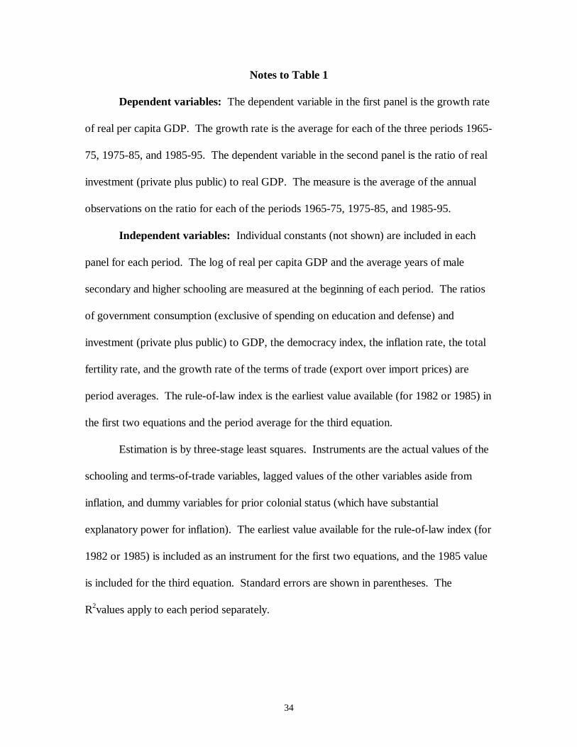
Notes to Table 1

Dependent variables: The dependent variable in the first panel is the growth rate

of real per capita GDP. The growth rate is the average for each of the three periods 1965-

75, 1975-85, and 1985-95. The dependent variable in the second panel is the ratio of real

investment (private plus public) to real GDP. The measure is the average of the annual

observations on the ratio for each of the periods 1965-75, 1975-85, and 1985-95.

Independent variables: Individual constants (not shown) are included in each

panel for each period. The log of real per capita GDP and the average years of male

secondary and higher schooling are measured at the beginning of each period. The ratios

of government consumption (exclusive of spending on education and defense) and

investment (private plus public) to GDP, the democracy index, the inflation rate, the total

fertility rate, and the growth rate of the terms of trade (export over import prices) are

period averages. The rule-of-law index is the earliest value available (for 1982 or 1985) in

the first two equations and the period average for the third equation.

Estimation is by three-stage least squares. Instruments are the actual values of the

schooling and terms-of-trade variables, lagged values of the other variables aside from

inflation, and dummy variables for prior colonial status (which have substantial

explanatory power for inflation). The earliest value available for the rule-of-law index (for

1982 or 1985) is included as an instrument for the first two equations, and the 1985 value

is included for the third equation. Standard errors are shown in parentheses. The

R2values apply to each period separately.

35

Table 2

Growth-Rate Forecasts

Country Growth forecast,1996-2006

Growth Rate,1960-95

Algeria 0.015 0.011Botswana -0.013 0.053 (6)Cameroon -0.001 0.012Congo (Republic) -0.038 0.015Egypt 0.029 0.026Gambia -0.007 0.005Ghana 0.019 0.002Kenya 0.013 0.008Malawi -0.005 0.007Mali 0.006 0.000Niger -0.021 -0.004Senegal 0.011 0.001Sierra Leone 0.007 -0.034*South Africa 0.009 0.010Sudan 0.005 0.008Togo 0.007 0.010Tunisia 0.030 0.030Uganda 0.014 0.003Zaire (Dem. Rep. of Congo) -0.016 -0.022Zambia 0.005 -0.016Zimbabwe 0.021 0.003Canada 0.007 0.025Costa Rica 0.020 0.018Dominican Republic 0.041 (5) 0.020El Salvador 0.016 0.012Guatemala 0.021 0.009Haiti 0.021 -0.016Honduras 0.029 0.009Jamaica 0.042 (4) 0.010Mexico 0.019 0.020Nicaragua 0.020 -0.008Panama 0.028 0.022Trinidad 0.009 0.010United States 0.011 0.019Argentina 0.032 0.007

36

Country Growth forecast,1996-2006

Growth Rate,1960-95

Bolivia 0.025 0.013Brazil 0.021 0.025Chile 0.030 0.020Colombia 0.022 0.023Ecuador 0.037 0.020Guyana 0.039 (9) -0.002Paraguay 0.029 0.018Peru 0.040 (8) 0.008Uruguay 0.014 0.008Venezuela 0.011 0.000Bangladesh -0.012 0.014China 0.053 (1) 0.039Hong Kong 0.012 0.059 (3)India 0.023 0.019Indonesia 0.027 0.041Iran 0.033 0.007Israel 0.010 0.032Japan 0.018 0.047 (8)Jordan 0.029 0.029South Korea 0.042 (3) 0.066 (1)Malaysia 0.019 0.045 (9)Pakistan 0.031 0.025Philippines 0.038 0.013Singapore 0.021 0.056 (4)Sri Lanka 0.045 (2) 0.019Syria 0.022 0.032Taiwan 0.019 0.061 (2)Thailand 0.037 0.048 (7)Austria 0.025 0.027Belgium 0.008 0.026Cyprus 0.014 0.044 (10)Denmark -0.010 0.023Finland -0.010 0.026France -0.002 0.026Germany -0.002 0.024Greece 0.040 (7) 0.035Hungary 0.039 (10) 0.017*Iceland -0.013 0.028Ireland 0.007 0.037Italy 0.015 0.030Malta 0.006 0.053 (5)Netherlands 0.014 0.024

37

Country Growth forecast,1996-2006

Growth Rate,1960-95

Norway -0.016 0.032Poland 0.041 (6) 0.014*Portugal 0.010 0.042Spain 0.024 0.034Sweden 0.000 0.019Switzerland 0.016 0.015Turkey 0.032 0.026United Kingdom 0.001 0.020Australia 0.001 0.021New Zealand 0.013 0.013Papua New Guinea 0.004 0.012

*1970-95

Note: The growth rate is the annual value for per capita real GDP. The forecasted valuefor 1996-2006 comes from the framework described in the text. The explanatory variablesused for most countries are the 1996 value of GDP, 1990 values of school attainment,1992 value of the government consumption ratio, 1997 value of rule of law, 1996 value ofdemocracy, 1996 value of fertility, 1996-97 value of inflation, and 1992 value of theinvestment ratio. Earlier values were used in some cases when the later data wereunavailable. The highest ten values in each column are indicated by the numbers shown inparentheses.

38

Table 3Contributions to Growth-Rate Predictions

Country Predictedgrowth rate

Contributionof log(GDP)

Contributionof schooling

Contributionof govt. con.

Contributionof rule of law

Contributionof fertility

Algeria -0.001 0.022 -0.006 -0.005 -0.005 -0.006Botswana -0.029 0.015 -0.012 -0.019 -0.001 -0.012Cameroon -0.017 0.035 -0.010 -0.010 -0.005 -0.019Congo (Republic) -0.054 0.028 0.001 -0.045 -0.005 -0.021Egypt 0.013 0.027 0.000 -0.004 -0.001 -0.005Gambia -0.023 0.035 -0.011 -0.024 0.002 -0.018Ghana 0.003 0.035 -0.004 -0.006 -0.005 -0.016Kenya -0.002 0.035 -0.011 -0.004 -0.001 -0.014Malawi -0.021 0.034 -0.012 -0.016 -0.001 -0.024Mali -0.010 0.034 -0.014 0.000 -0.005 -0.025Niger -0.037 0.032 -0.014 -0.012 -0.008 -0.027Senegal -0.005 0.035 -0.011 -0.005 -0.005 -0.020Sierra Leone -0.009 0.035 -0.011 -0.004 -0.005 -0.024South Africa -0.006 0.017 -0.006 -0.007 -0.005 -0.001Sudan -0.011 0.035 -0.010 -0.002 -0.008 -0.015Togo -0.008 0.034 -0.006 -0.006 -0.005 -0.022Tunisia 0.014 0.015 -0.005 0.003 0.002 0.000Uganda -0.002 0.035 -0.014 0.001 -0.001 -0.024Zaire -0.032 0.019 -0.010 0.001 -0.008 -0.023Zambia -0.011 0.034 -0.008 -0.015 -0.001 -0.020Zimbabwe 0.005 0.034 -0.012 -0.008 -0.001 -0.009Canada -0.009 -0.058 0.019 0.011 0.006 0.014Costa Rica 0.004 0.011 -0.003 -0.001 -0.001 0.000Dominican Republic 0.026 0.022 -0.005 0.007 -0.001 -0.003El Salvador 0.000 0.026 -0.007 -0.009 -0.005 -0.006Guatemala 0.005 0.025 -0.010 0.007 -0.005 -0.014Haiti 0.005 0.034 -0.010 -0.004 -0.005 -0.012Honduras 0.013 0.032 -0.008 0.004 -0.005 -0.013Jamaica 0.026 0.023 -0.005 0.007 -0.005 0.005Mexico 0.003 -0.004 0.001 0.009 -0.005 0.001Nicaragua 0.004 0.034 -0.008 -0.012 -0.001 -0.010Panama 0.012 0.014 0.006 -0.008 -0.005 0.002Trinidad -0.007 -0.017 0.000 0.007 -0.001 0.008United States -0.005 -0.064 0.034 0.013 0.006 0.008Argentina 0.016 -0.003 -0.001 0.015 0.002 0.001Bolivia 0.009 0.029 -0.001 0.000 -0.005 -0.013Brazil 0.005 0.008 -0.007 0.005 -0.005 0.004Chile 0.015 -0.005 0.000 0.008 0.002 0.006Colombia 0.006 0.012 -0.005 0.005 -0.008 0.001Ecuador 0.021 0.019 0.002 0.005 -0.001 -0.003Guyana 0.023 0.032 -0.006 -0.007 -0.001 0.005

39

Country Predictedgrowth rate

Contributionof log(GDP)

Contributionof schooling

Contributionof govt. con.

Contributionof rule of law

Contributionof fertility

Paraguay 0.013 0.026 -0.006 0.000 -0.001 -0.010Peru 0.024 0.021 0.000 0.006 -0.005 -0.003Uruguay -0.002 -0.001 0.001 0.001 -0.005 0.007Venezuela -0.005 -0.005 -0.004 0.007 -0.001 -0.002Bangladesh -0.028 0.031 -0.007 -0.040 -0.005 -0.005China 0.037 0.024 0.002 0.002 0.002 0.011Hong Kong -0.003 -0.061 0.016 0.013 0.002 0.023India 0.007 0.031 -0.004 -0.016 -0.001 -0.003Indonesia 0.012 0.021 -0.008 0.003 -0.001 0.002Iran 0.017 0.012 -0.003 0.014 0.002 -0.009Israel -0.006 -0.031 0.007 0.015 0.002 0.002Japan 0.003 -0.052 0.016 0.012 0.006 0.019Jordan 0.014 0.016 0.008 0.000 -0.001 -0.013South Korea 0.026 -0.026 0.021 0.015 -0.001 0.013Malaysia 0.003 -0.013 0.002 0.010 0.002 -0.005Pakistan 0.015 0.031 -0.002 0.002 -0.001 -0.017Philippines 0.022 0.029 0.000 0.001 -0.001 -0.008Singapore 0.005 -0.036 0.000 0.014 0.006 0.014Sri Lanka 0.029 0.023 0.001 -0.002 -0.001 0.006Syria 0.006 0.004 0.001 0.015 0.002 -0.010Taiwan 0.003 -0.033 0.012 0.010 -0.001 0.012Thailand 0.021 0.000 -0.006 0.006 0.002 0.012Austria 0.009 -0.043 0.021 0.007 0.006 0.019Belgium -0.008 -0.045 0.008 0.012 0.002 0.016Cyprus -0.001 -0.025 0.010 0.005 0.002 0.008Denmark -0.026 -0.051 0.009 0.000 0.006 0.012Finland -0.025 -0.044 0.000 0.002 0.006 0.012France -0.017 -0.047 0.007 0.008 0.002 0.013Germany -0.018 -0.049 -0.002 0.006 0.006 0.022Greece 0.024 -0.012 0.007 0.009 0.002 0.020Hungary 0.023 0.001 -0.002 0.002 0.006 0.018Iceland -0.029 -0.044 0.008 -0.005 0.006 0.008Ireland -0.009 -0.040 0.007 0.009 0.006 0.011Italy -0.001 -0.042 0.006 0.006 0.006 0.023Malta -0.010 -0.020 -0.002 -0.004 0.006 0.012Netherlands -0.002 -0.046 0.012 0.012 0.006 0.017Norway -0.032 -0.060 0.008 0.005 0.006 0.011Poland 0.025 0.007 0.001 0.002 0.002 0.015Portugal -0.006 -0.018 -0.004 -0.002 0.002 0.019Spain 0.008 -0.029 0.005 0.007 0.002 0.023Sweden -0.016 -0.048 0.017 -0.002 0.006 0.013Switzerland 0.000 -0.051 0.016 0.012 0.006 0.017Turkey 0.016 0.009 -0.005 0.011 -0.001 0.002United Kingdom -0.016 -0.045 0.007 0.006 0.006 0.014Australia -0.015 -0.055 0.015 0.008 0.006 0.012New Zealand -0.003 -0.039 0.016 0.006 0.006 0.009Papua New Guinea -0.012 0.028 -0.012 -0.009 -0.005 -0.015

40

Note: The predicted growth rate for 1996-2006 is expressed as a deviation from thesample mean (which was 0.016). The other columns show the contribution to the growth-rate prediction from the indicated independent variable. The contribution equals therespective coefficient estimate multiplied by the value of the independent variable(expressed as a deviation from the sample mean).

41

Table 4

Growth Rates for 1985-95

Country Growth rate,1985-95

Predictedgrowth rate

Algeria -0.018 0.006Botswana 0.037 0.008Cameroon -0.043 0.014Congo (Republic) -0.035 -0.021Egypt 0.004 0.021Gambia -0.007 0.000Ghana 0.020 -0.005Kenya 0.008 0.018Liberia ---- 0.006Malawi -0.005 -0.004Mali -0.001 0.005Niger -0.020 0.003Senegal -0.008 0.003Sierra Leone -0.038 -0.003South Africa -0.007 0.008Sudan 0.015 0.008Togo -0.021 0.008Tunisia 0.015 0.020Uganda 0.019 0.001Zaire -0.068 -0.006Zambia -0.038 -0.012Zimbabwe -0.012 0.022Canada 0.011 0.008Costa Rica 0.021 0.011Dominican Republic 0.013 0.026El Salvador 0.017 0.001Guatemala 0.008 0.013Haiti -0.053 0.004Honduras 0.002 0.018Jamaica 0.014 0.026Mexico 0.001 0.008Nicaragua -0.040 0.011Panama -0.002 0.005Trinidad -0.021 -0.006United States 0.013 0.019Argentina 0.006 0.009

42

Country Growth rate,1985-95

Predictedgrowth rate

Bolivia 0.001 0.001Brazil 0.006 0.021Chile 0.050 0.034Colombia 0.024 0.017Ecuador 0.000 0.028Guyana 0.017 0.018Paraguay 0.005 0.023Peru 0.004 0.023Uruguay 0.029 0.022Venezuela 0.002 0.006Bangladesh 0.025 -0.013China 0.057 0.049Hong Kong 0.053 0.030India 0.034 0.013Indonesia 0.047 0.031Iran -0.008 0.009Iraq ---- -0.006Israel 0.026 0.007Japan 0.025 0.017Jordan -0.012 0.017South Korea 0.077 0.065Kuwait ---- -0.015Malaysia 0.052 0.040Pakistan 0.019 0.027Philippines 0.013 0.019Singapore 0.032 0.032Sri Lanka 0.018 0.032Syria 0.011 0.015Taiwan 0.067 0.052Thailand 0.072 0.032Austria 0.018 0.028Belgium 0.020 0.015Cyprus 0.039 0.014Denmark 0.015 -0.007Finland 0.009 0.003France 0.016 0.008Germany 0.018 -0.011Greece 0.013 0.029Hungary -0.004 0.033Iceland 0.007 -0.008Ireland 0.050 0.015Italy 0.019 0.009

43

Country Growth rate,1985-95

Predictedgrowth rate

Malta 0.049 0.006Netherlands 0.019 0.020Norway 0.020 -0.003Poland 0.000 0.032Portugal 0.046 0.023Spain 0.030 0.020Sweden 0.008 0.000Switzerland 0.006 0.016Turkey 0.026 0.029United Kingdom 0.020 -0.008Yugoslavia ---- 0.023Australia 0.017 0.012New Zealand 0.008 0.017Papua New Guinea 0.015 0.007

Note: The growth rate is for per capita GDP from 1985 to 1995. The predicted growthrate is the forecast based on data through 1985.

44

References

Barro, Robert J. (1997). Determinants of Economic Growth: A Cross-Country

Empirical Study, Cambridge MA, MIT Press.

Barro, Robert J. and Jong-Wha Lee (1997). “Determinants of Schooling Quality,”

unpublished, Harvard University, March.

Barro, Robert J. and Xavier Sala-i-Martin (1995). Economic Growth, New York,

McGraw Hill.

Bollen, Kenneth A. (1990). “Political Democracy: Conceptual and Measurement Traps,”

Studies in Comparative International Development, Spring, 7-24.

Cass, David (1965). “Optimum Growth in an Aggregative Model of Capital

Accumulation,” Review of Economic Studies, 32 (July), 233-240.

Easterly, William and Sergio Rebelo (1993). “Fiscal Policy and Economic Growth: An

Empirical Investigation,” Journal of Monetary Economics, 32, 3 (December),

417-458.

Gastil, Raymond D. (1982-83 and other years). Freedom in the World, Westport CT,

Greenwood Press.

Hanushek, Eric and Dongwook Kim (1995). “Schooling, Labor Force Quality, and

Economic Growth,” Rochester Center for Economic Research, working paper no.

411, September.

Inkeles, Alex (1991). On Measuring Democracy, New Brunswick NJ, Transaction

Publishers.

International Labour Organization (1990). Summaries of International Labour

45

Standards, 2nd edition, Geneva, International Labour Office.

International Labour Organization (1995). Lists of Ratification by Convention and by

Country, Geneva, International Labour Office.

King, Robert G. and Ross Levine (1993). “Finance, Entrepreneurship, and Growth:

Theory and Evidence,” Journal of Monetary Economics, 32, 3 (December),

513-542.

Knack, Stephen and Philip Keefer (1995). “Institutions and Economic Performance:

Cross-Country Tests Using Alternative Institutional Measures,” Economics and

Politics, 7, 207-227.

Koopmans, Tjalling C. (1965). “On the Concept of Optimal Economic Growth,” in The

Econometric Approach to Development Planning, Amsterdam, North Holland.

Rodrik, Dani (1996). “Labor Standards in International Trade: Do They Matter and

What Do We Do about Them?,” unpublished, Harvard University, May.

Ramsey, Frank (1928). “A Mathematical Theory of Saving,” Economic Journal, 38

(December), 543-559.

Romer, Paul M. (1990). “Endogenous Technological Change,” Journal of Political

Economy, 98, 5 (October), part II, S71-S102.

Sachs, Jeffrey D. and Andrew Warner (1995). “Economic Reform and the Process of

Global Integration,” Brookings Papers on Economic Activity, no. 1, 1-95.

Solow, Robert M. (1956). “A Contribution to the Theory of Economic Growth,”

Quarterly Journal of Economics, 70, 1 (February), 65-94.

Summers, Robert, and Alan Heston (1991). “The Penn World Table (Mark 5): An

46

Expanded Set of International Comparisons, 1950-1988,” Quarterly Journal of

Economics, 106, 2 (May), 327-369.

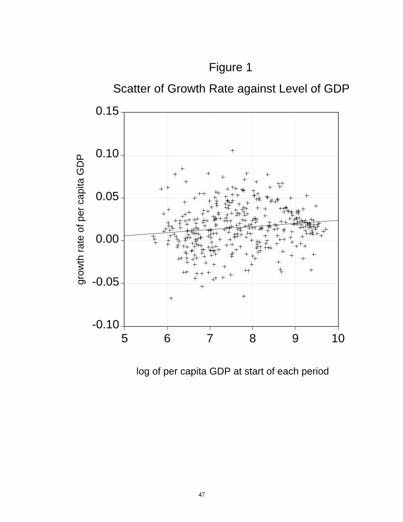
47

-0.10

-0.05

0.00

0.05

0.10

0.15

5 6 7 8 9 10

grow

th r

ate

of p

er c

apita

GD

P

log of per capita GDP at start of each period

Scatter of Growth Rate against Level of GDP

Figure 1

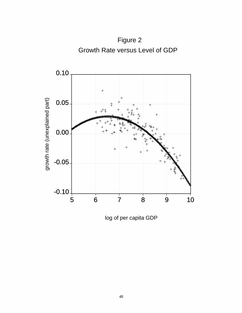
48

-0.10

-0.05

0.00

0.05

0.10

5 6 7 8 9 10

grow

th r

ate

(une

xpla

ined

par

t)

log of per capita GDP

-0.10

-0.05

0.00

0.05

0.10

5 6 7 8 9 10

Growth Rate versus Level of GDP

Figure 2

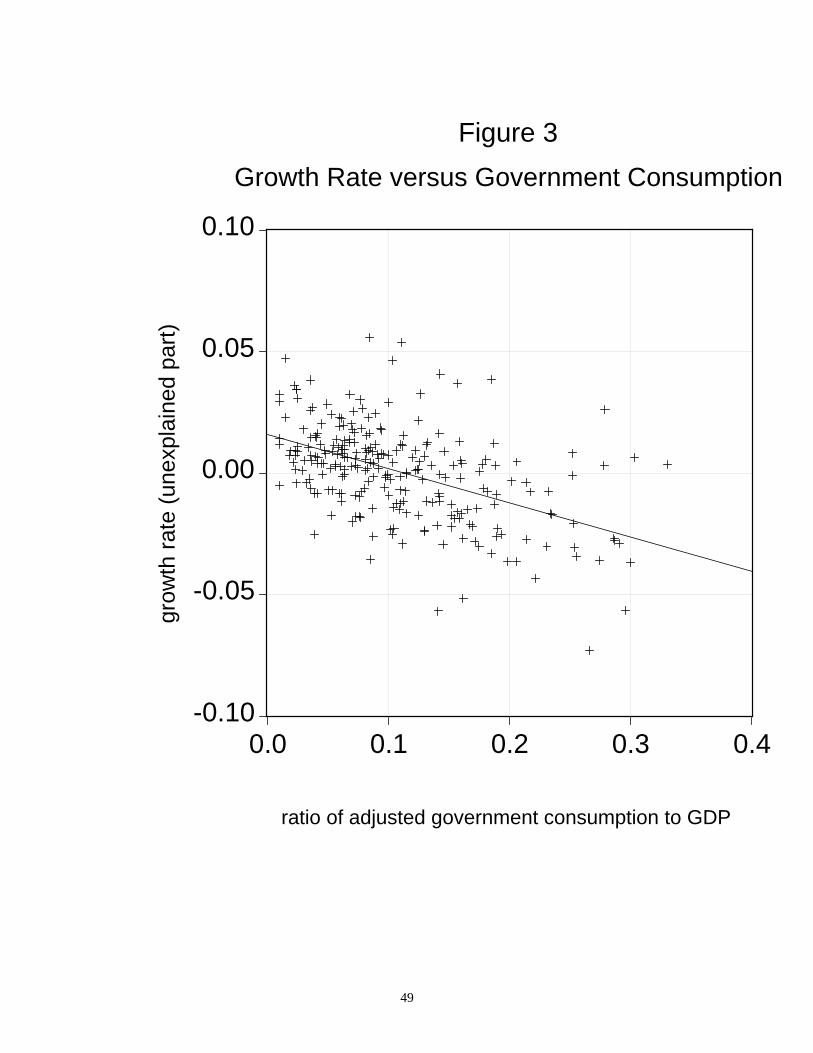
49

-0.10

-0.05

0.00

0.05

0.10

0.0 0.1 0.2 0.3 0.4

grow

th r

ate

(une

xpla

ined

par

t)

ratio of adjusted government consumption to GDP

Growth Rate versus Government Consumption

Figure 3

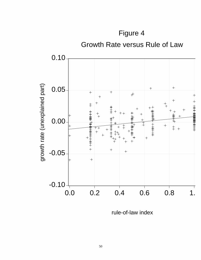
50

-0.10

-0.05

0.00

0.05

0.10

0.0 0.2 0.4 0.6 0.8 1.

grow

th r

ate

(une

xpla

ined

par

t)

rule-of-law index

Growth Rate versus Rule of Law

Figure 4

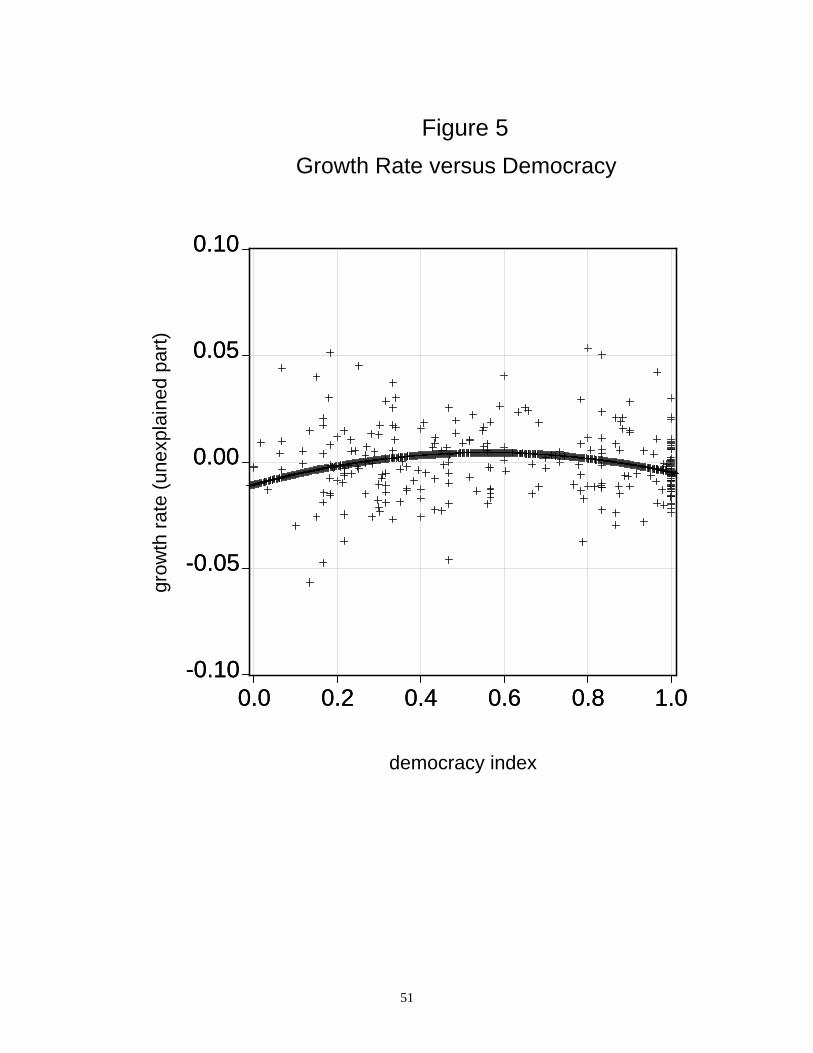
51

-0.10

-0.05

0.00

0.05

0.10

0.0 0.2 0.4 0.6 0.8 1.0

grow

th r

ate

(une

xpla

ined

par

t)

democracy index

-0.10

-0.05

0.00

0.05

0.10

0.0 0.2 0.4 0.6 0.8 1.0

Growth Rate versus Democracy

Figure 5

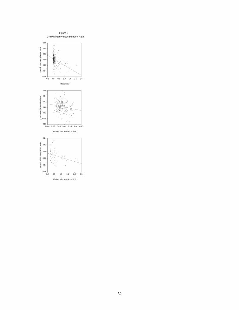
52

-0.06

-0.04

-0.02

0.00

0.02

0.04

0.06

-0.5 0.0 0.5 1.0 1.5 2.0 2.5

grow

th r

ate

(une

xpla

ined

par

t)

inflation rate

-0.06

-0.04

-0.02

0.00

0.02

0.04

0.06

-0.05 0.00 0.05 0.10 0.15 0.20 0.25

grow

th r

ate

(une

xpla

ined

par

t)

inflation rate, for rates < 20%

-0.06

-0.04

-0.02

0.00

0.02

0.04

0.0 0.5 1.0 1.5 2.0 2.5

grow

th r

ate

(une

xpla

ined

par

t)

inflation rate, for rates > 20%

Growth Rate versus Inflation Rate

Figure 6

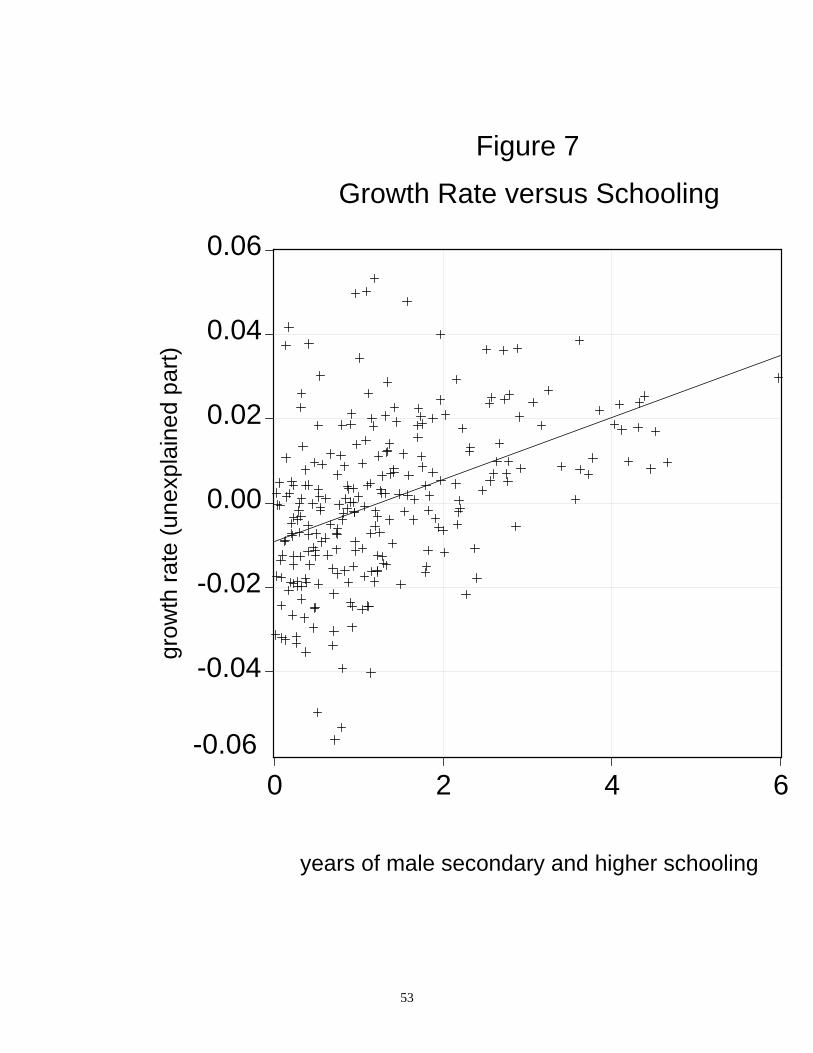
53

-0.04

-0.02

0.00

0.02

0.04

0.06

0 2 4 6

grow

th r

ate

(une

xpla

ined

par

t)

years of male secondary and higher schooling

Growth Rate versus Schooling

Figure 7

-0.06

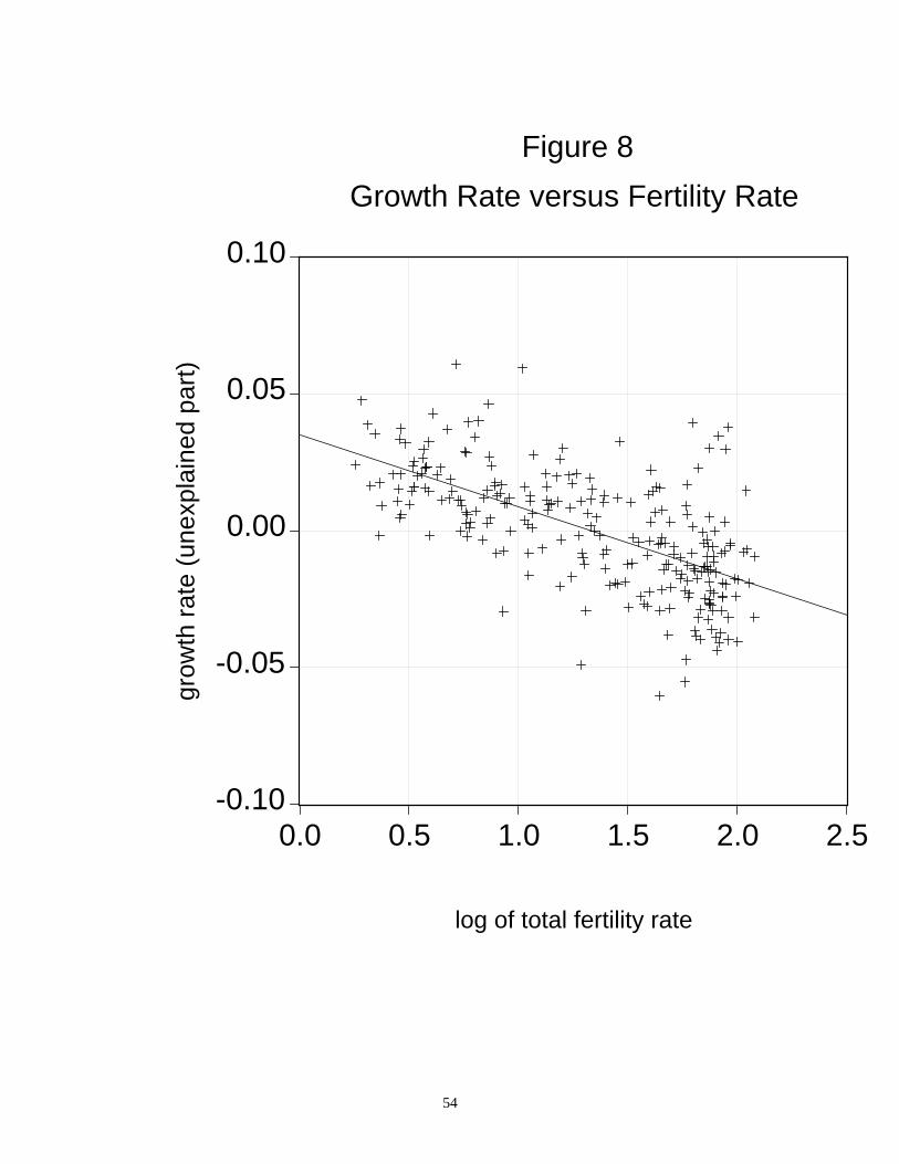
54

-0.10

-0.05

0.00

0.05

0.10

0.0 0.5 1.0 1.5 2.0 2.5

grow

th r

ate

(une

xpla

ined

par

t)

log of total fertility rate

Growth Rate versus Fertility Rate

Figure 8

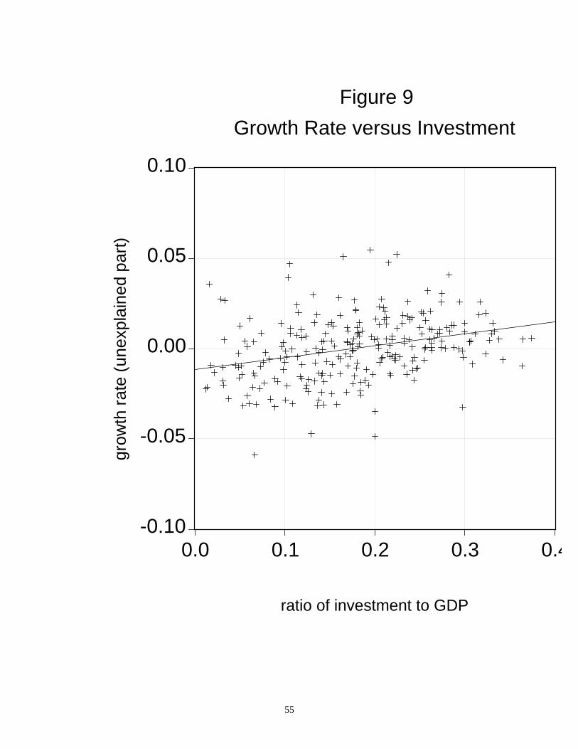
55

-0.10

-0.05

0.00

0.05

0.10

0.0 0.1 0.2 0.3 0.4

grow

th r

ate

(une

xpla

ined

par

t)

ratio of investment to GDP

Growth Rate versus Investment

Figure 9

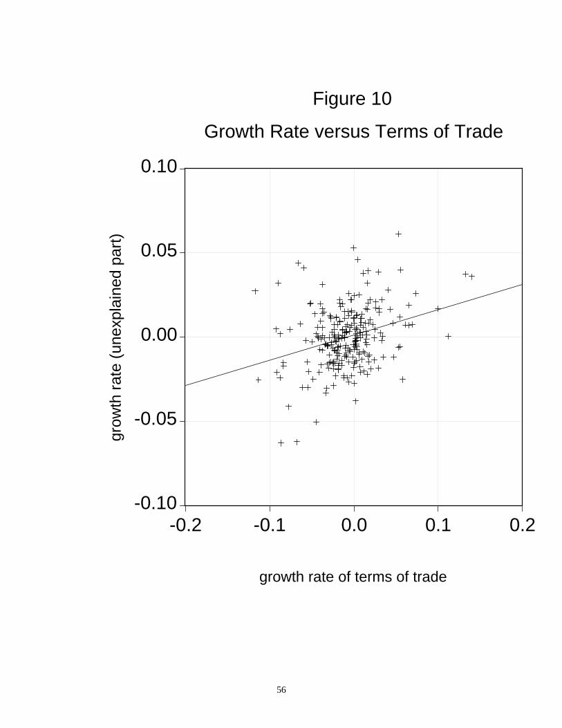
56

-0.10

-0.05

0.00

0.05

0.10

-0.2 -0.1 0.0 0.1 0.2

grow

th r

ate

(une

xpla

ined

par

t)

growth rate of terms of trade

Growth Rate versus Terms of Trade

Figure 10