Human capital and growth - UNU-WIDER · 1957 E St. NW, Suite 502 Voice: (202) 994-5320 ... 2007; Lobell, Schlenker, and Costa-Roberts, 2011; Schlenker and Lobell, 2010; Guiteras,

DRAFTThis paper is a draft submission to the

This is a draft version of a conference paper submitted for presentation at UNU-WIDER’s conference, held in Helsinki on 6-7 June 2016. This is not a formal publication of UNU-WIDER and may refl ect work-in-progress.

Human capital and growth6-7 June 2016 Helsinki, Finland

THIS DRAFT IS NOT TO BE CITED, QUOTED OR ATTRIBUTED WITHOUT PERMISSION FROM AUTHOR(S).

WIDER Development Conference

Institute for International Economic Policy Working Paper Series

Elliott School of International Affairs

The George Washington University

Long-Term Impacts of High Temperatures on Economic

Productivity

IIEP-WP-2015-18

Ram Fishman

Jason Russ

Paul Carrillo

George Washington University

October 2015

Institute for International Economic Policy

1957 E St. NW, Suite 502

Voice: (202) 994-5320

Fax: (202) 994-5477

Email: [email protected]

Web: www.gwu.edu/~iiep

http://www.gwu.edu/~iiep

mailto:[email protected]

1

Long-Term Impacts of High Temperatures on Economic Productivity Ram Fishman*

Jason Russ**

Paul Carrillo***

DRAFT: October 2015

A substantial body of recent evidence on the socio-economic and health related impacts of high temperature anomalies, alongside the literature on the long-term impacts of in-utero stress on adult welfare (the fetal origins hypothesis), suggests that exposure to high temperature anomalies in-utero may have long-term impacts on adult human capital accumulation and economic productivity. To test this hypothesis, we match and regress administrative data on the 2010 earnings of all formal sector workers in Ecuador (over 1.5 million individuals born between 1950 and 1989) on temperature and rainfall anomalies in and around the time of each individual’s birth, at the location of birth. We find that higher temperatures while in-utero lead to significantly lower earnings, especially for women, for whom a 1°C increase in temperature leads to a 1.1%-1.7% decrease in earnings. The results are robust to the inclusion of rich sets of flexible controls and a range of falsification tests., and suggest climate change may already have caused adverse long-term �pipeline� economic impacts that have not been appreciated to date.

Keywords: Climate Change, Economic Impacts, Fetal Origins

JEL Codes: J31, Q50

Acknowledgments: we are grateful for support by the Institute for International Economic Policy at George Washington University. This paper has benefited from comments and suggestions by seminar participants at George Washington University, Aalto University, UC Berkeley, the Hebrew University of Jerusalem and the Washington Area Development Economics Conference. ____________________________________________

* George Washington University. Contact Email: [email protected] ** George Washington University. Contact Email: [email protected] ***George Washington University. Contact Email: [email protected]

2

Growing interest in the future impacts of climate change has spurred a burgeoning

literature on the economic impacts of high temperatures (see Dell et al, 2012, for a review).

Multiple analyses of historical weather and socio-economic data have now produced a

substantial body of robust evidence that high temperature anomalies lead to a range of adverse

social and economic impacts, including reductions in economic productivity and growth in both

the agricultural and non-agricultural sectors (Deschenes and Greenstone, 2007; Lobell,

Schlenker, and Costa-Roberts, 2011; Schlenker and Lobell, 2010; Guiteras, 2009; Fishman,

2011; Hsiang, 2010; Dell et al, 2012; Sudarshan and Tewari, 2011; Zivin and Neidel, 2014;

Deryugina and Hsiang, 2014), increases in morbidity (Burgess et al, 2011; Patz et al, 2005;

McMichael, Woodruff, and Hales, 2006 ), crime and conflict (Hsiang, Burke and Miguel 2013;

Ranson 2012; Blakeslee and Fishman 2013).

Another, independent body of evidence establishes the long-term impacts of early life

stress on adult socio-economic indicators, health and well-being. In particular, the fetal origins

hypothesis posits that in-utero circumstances can have substantial long-term impacts on human

development. Numerous studies have provided evidence in support of this hypothesis, finding

that economic, environmental or disease-related stress in infancy or in-utero lead to long-term

impacts on physical and cognitive health, educational attainment and wages (Almond and Curie,

2011). When combined with the evidence on the multiple socio-economic and health related

impacts of high temperature anomalies, this suggests that individuals who are exposed to high

ambient temperatures in-utero or in infancy may experience life-long negative consequences

through a number of possible channels, both physiological and economic (for example, declines

in income or economic hardship can reduce consumption of crucial nutritional inputs by

pregnant women). This, in turn, would suggest that the warming that has already taken places in

the past few decades may incur hitherto under-appreciated, long-term economic losses. To the

best of our knowledge, this paper provides the first body of empirical evidence on this possible

important long-term linkage.

In this paper, we investigate the effect of high temperature anomalies around the time of

birth on formal earnings as an adult. Economic theory suggests that in well functioning markets,

wages provide an accurate indicator of economic productivity and human capital, including

physical and cognitive function. A relationship between temperature anomalies in-utero and

3

adult earnings would therefore measure the total economic losses associated with long-term

human capital losses resulting from stress in-utero, even if the contribution of each potential

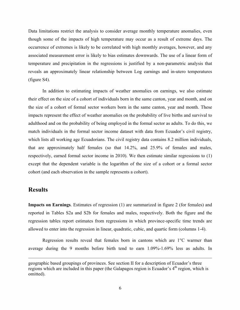
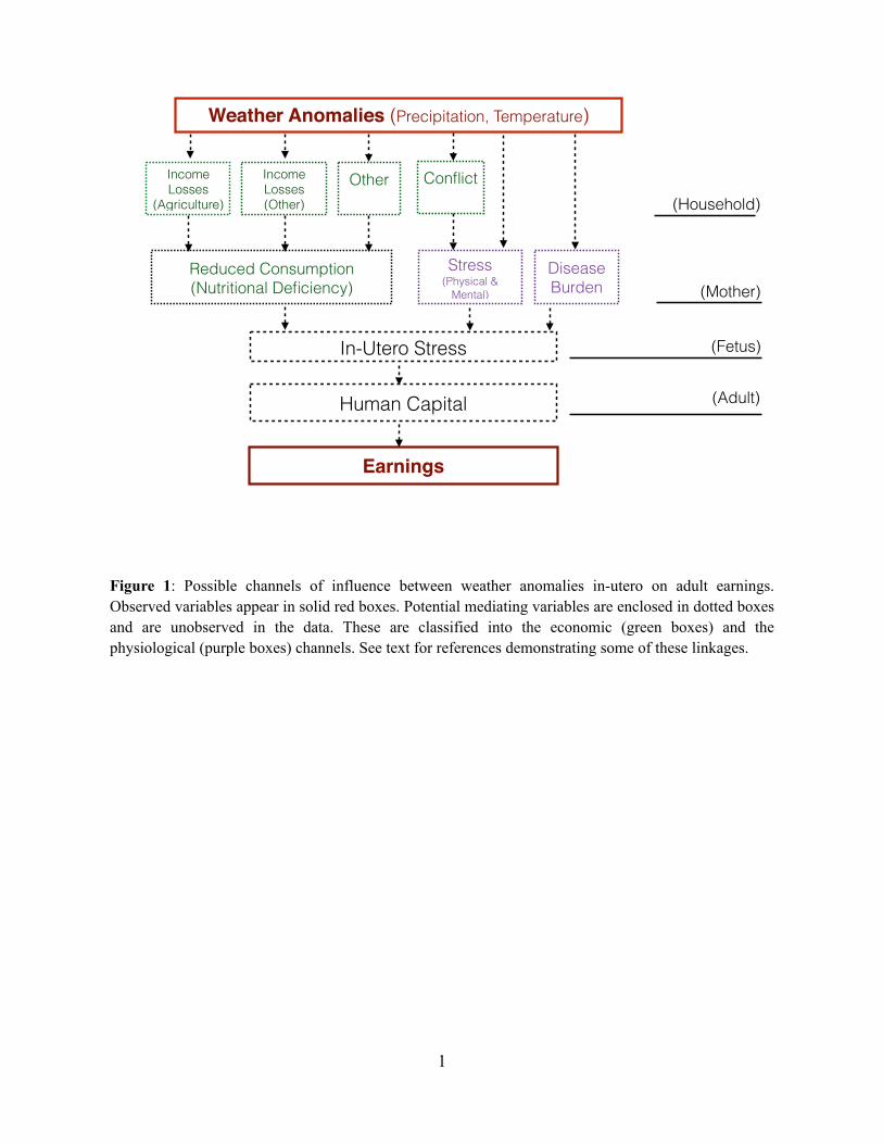
channel of causation may not be possible to measure directly (figure 1).

Our analysis makes use of a unique data set on the 2010 earnings of all 1.5 million formal

sector workers in Ecuador, born between 1950 and 1989, that was merged with civil registry data

to identify the place and time of birth of these individuals, and then merged with historical

weather data sets to identify temperature and precipitation levels around the time of birth

(including in-utero). A regression analysis of the relationship between adult earnings and

temporal temperature anomalies revealed that higher temperatures in-utero lead to significantly

lower adult earnings for women, with a 1°C increase in average monthly temperature in-utero

leading to a 1.1%-1.7% decrease in adult earnings. These results are highly robust to the

inclusion of fine geographic controls, localized annual cycles and time trends, and to various

falsification tests. Even though the reduced-form analysis does not allow us to identify which of

the established negative impacts of high temperatures is driving the association, the random

nature of temperature variations over time within a geographical locality facilitates causal

inference (Dell et al, 2012).

Several previous studies have used a similar methodology to find long-term impacts of

drought or floods at the year of birth on the welfare, physical and cognitive health of farming

households in low-income countries (Maccini and Yang, 2008; Aguilar and Vicarelli, 2011;

Tiwari et al, 2013). We believe this study to be the first to focus on temperature anomalies, or to

relate weather anomalies to administrative formal earning data. In addition, our sample consists

of adults born in both urban and rural areas that are employed in the formal sector of a middle-

income economy, and therefore have higher earnings and education levels than the samples

studied in previous studies. Our findings are consistent with a small number of other studies that

have found detrimental short-term impacts of high temperatures in-utero on post-birth health

outcomes. For example, birthweight in the U.S. is found to be negatively correlated with in-utero

exposure to high temperatures (Deschens, Greenstone and Guryan, 2009). However, we extend

these results by observing much longer-term, economic impacts.

4

Materials and Methods

Data: Ecuador is a relatively small, middle-income country in South America with a

population of about 16 million residents. Over the time period in which our sample was born,

GDP per capita has increased significantly, and at the same time, infant mortality has fallen

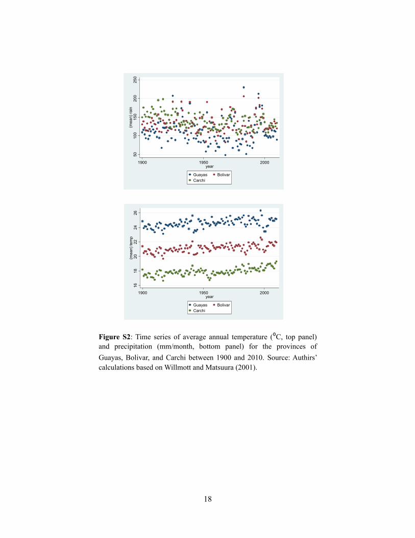
precipitously (Figure S1). Despite its small size, Ecuador’s weather patterns display a large

degree of spatial and temporal variation (Figure S2).

Earnings data were obtained from the Ecuadorian Tax Authority. This dataset contains

the 2010 annual earnings of all Ecuadorians working in the formal sector, i.e. all workers

employed in firms that report corporate tax returns to the Tax Authority. The Tax Authority

complemented their earnings data with information from the National Civil Registry, which

includes several demographic characteristics of workers including their gender, year and month

of birth, place of birth (at the level of a canton, a small political administrative unit of which

there are 218 in Ecuador, and educational attainment. Our sample includes individuals born

between the year 1950 and 1989, implying that all individuals in our dataset are between 21 and

60 years old at the time their earnings are reported. Unfortunately, the data does not allow us to

group individuals by family unit.

Precipitation and Temperature data is based on the 1900-2010 Gridded Monthly Time

Series on Terrestrial Air Temperature, and the 1900-2010 Gridded Monthly Time Series on

Terrestrial Precipitation from the University of Delaware (Willmott and Matsuura, 2001). The

gridded data was used to calculate monthly temperature and precipitation in each of Ecuador’s

218 Cantons through spatial averaging (see the SI section and figure S3). Summary statistics for

the earnings and weather data are given in Table S1.

Regression Analysis: We employ regression analysis to investigate the correlation

between in-utero weather and adult earnings. Regressing adult earnings on weather patterns

across geographical locations of birth can generate biased estimates because of potential

unobservable confounding variables. We therefore follow previous studies (Dell et al, 2012) and

base our estimates on local temporal deviations of weather from the local long-term mean in

each locality. Such deviations are likely to be random and therefore orthogonal to any possible

confounders, facilitating causal inference. To isolate these localized temporal fluctuations in

5

weather, we include location (canton) fixed effects and year fixed effects in the regressions (the

latter flexibly control for annual variation in weather that affects the entire country such as

ENSO). Similarly, given the long time span over which individuals in our earnings data are born,

it is also important to control for time-trends in the regression. Otherwise, unrelated trends in

weather (such as warming), socio-economic circumstances (due to economic growth) and 2010

earnings (due to age effects) can result in spurious correlations. To adequately capture these

potentially confounding trends in observable and unobservable variables, our regressions include

highly flexible, localized time trends which we allow to vary from linear to quartic in each of

Ecuador’s 24 provinces. In the same vein, we include fixed-effects for every combination of

canton and month (1-12) of birth in order to ensure estimates are not driven by potentially biased

correlations between the month of birth and local seasonal patterns that can also lead to spurious

correlations. The inclusion of this rich set of controls assures that regression estimates are based

solely on temporal random fluctuations in monthly temperature within each locale. Our main

model specification therefore takes the following form:

!"(!!"#$) = !! + !!!!"#! + !!!!"#! + !!!!"#! + !!!!"#!! + !!(!) + !!" + !! + !! (1)

where is (log) income of individual i, born in canton c, in month m of year y;!!!"#! and !!"#! are

the average temperature (in degrees Celsius) in the canton of birth for the 9 months before birth,

and the 9 months after birth, respectively, and !!"#! and !!"#!! !are the average monthly

precipitation (cm) in the canton of birth for the 9 months before birth, and the 9 months after

birth, respectively; !!(!) is a province specific time trend (ranging from linear to quartic

specifications); !!" are month-canton fixed effects that capture any unobserved characteristics

of every combination of a canton and month of year, such as location specific seasonal cycles;

and !! are year fixed effects. To account for possible serial or spatial correlations amongst

observations, we cluster our main results at several different levels: canton, province-year,

region-year1 and province, but find little impact on the significance of our estimates. Subsequent

results have errors conservatively clustered at the province level.

1 Provinces are Ecuador’s largest political unit. There are 24 provinces in Ecuador, including the Galapagos province, which is excluded from our study, leaving 23 provinces. Cantons are the second largest political unit. Our dataset consists of births from 218 cantons. Regions are

6

Data limitations restrict the analysis to consider average monthly temperature anomalies, even

though some of the impacts of high temperature may occur as a result of extreme days. The

occurrence of extremes is likely to be correlated with high monthly averages, however, and any

associated measurement error is likely to bias estimates downwards. The use of a linear form of

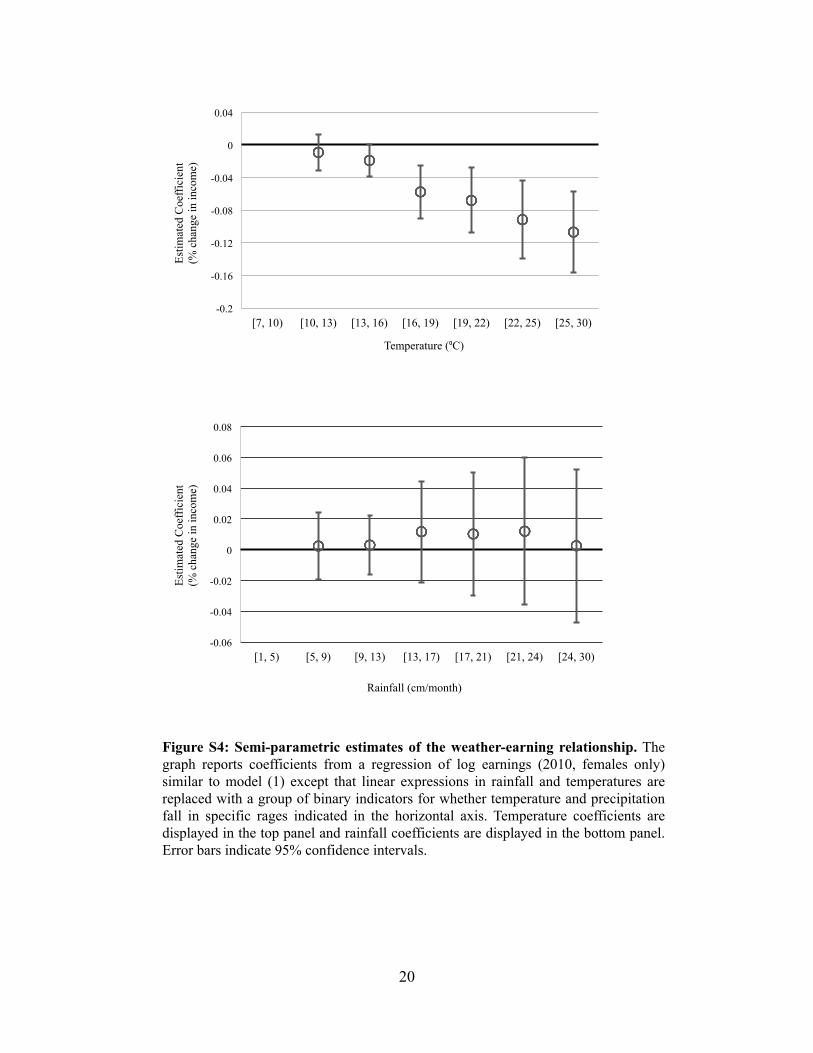
temperature and precipitation in the regressions is justified by a non-parametric analysis that

reveals an approximately linear relationship between Log earnings and in-utero temperatures

(figure S4).

In addition to estimating impacts of weather anomalies on earnings, we also estimate

their effect on the size of a cohort of individuals born in the same canton, year and month, and on

the size of a cohort of formal sector workers born in the same canton, year and month. These

impacts represent the effect of weather anomalies on the probability of live births and survival to

adulthood and on the probability of being employed in the formal sector as adults. To do this, we

match individuals in the formal sector income dataset with data from Ecuador’s civil registry,

which lists all working age Ecuadorians. The civil registry data contains 8.2 million individuals,

that are approximately half females (so that 14.2%, and 25.9% of females and males,

respectively, earned formal sector income in 2010). We then estimate similar regressions to (1)

except that the dependent variable is the logarithm of the size of a cohort or a formal sector

cohort (and each observation in the sample represents a cohort).

Results

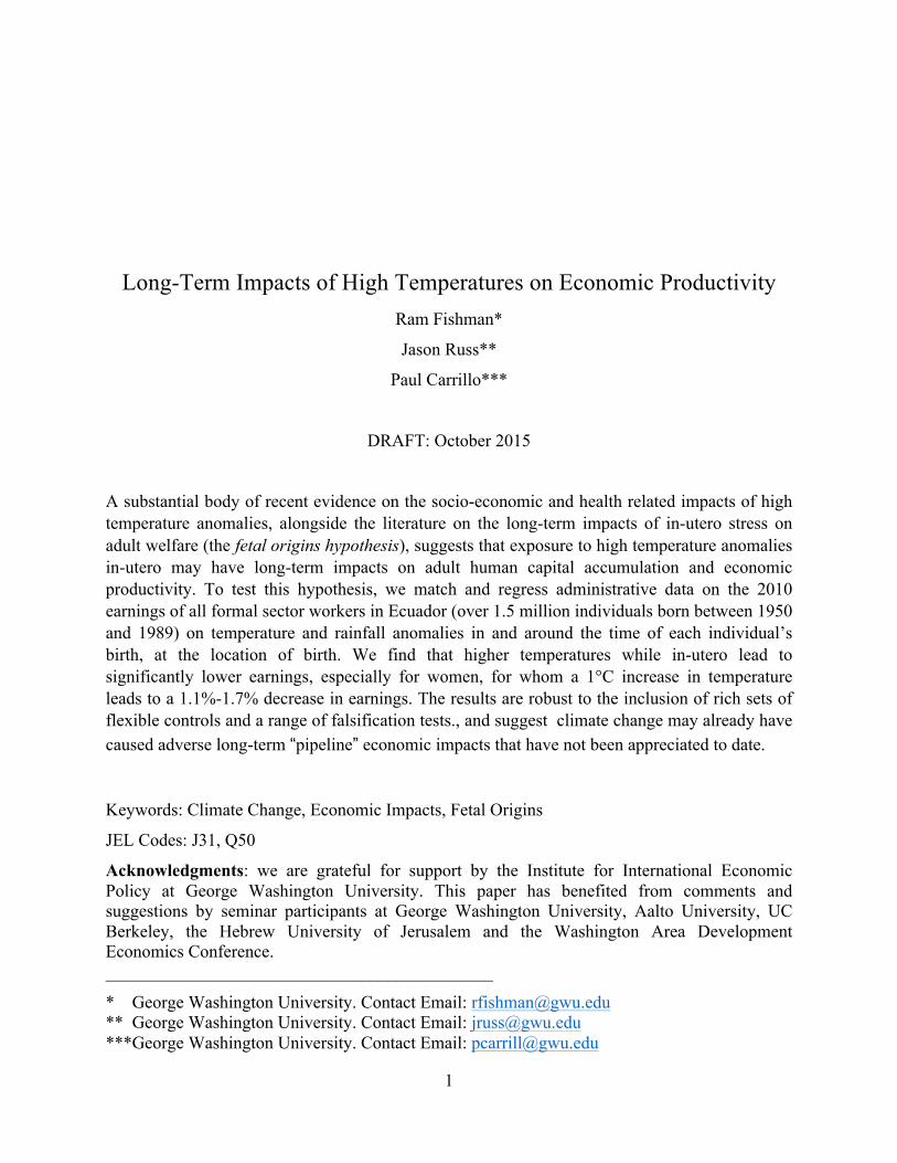
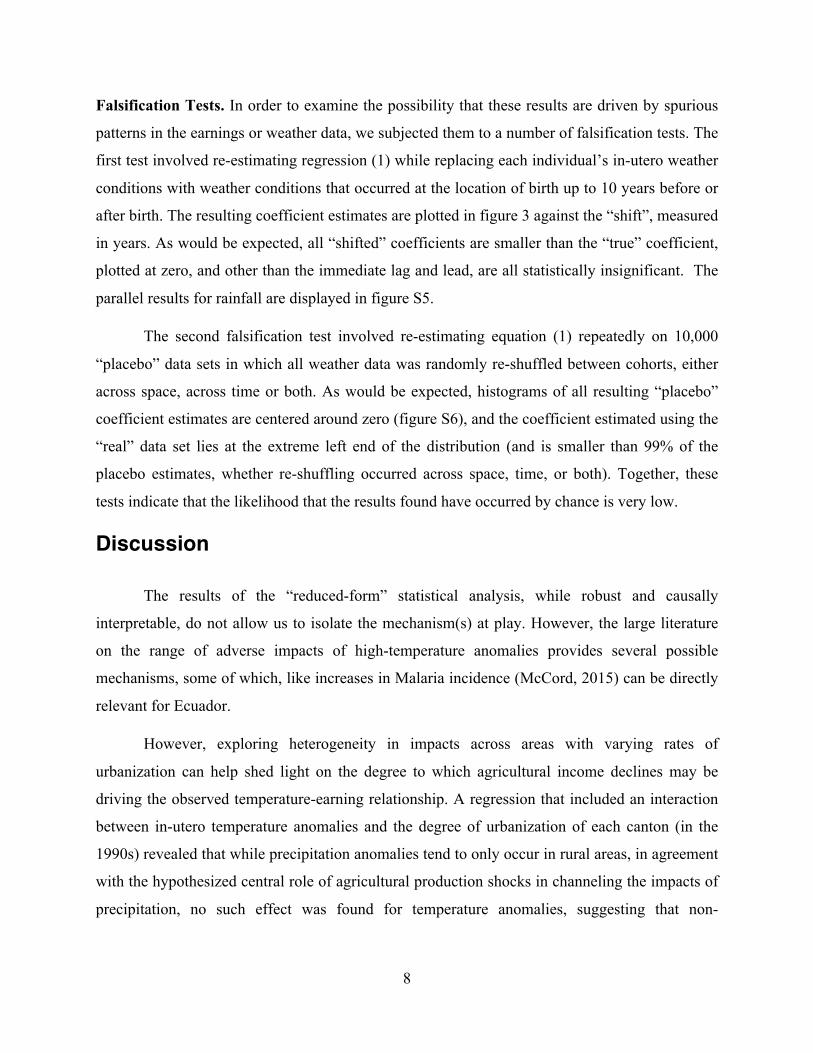
Impacts on Earnings. Estimates of regression (1) are summarized in figure 2 (for females) and

reported in Tables S2a and S2b for females and males, respectively. Both the figure and the

regression tables report estimates from regressions in which province-specific time trends are

allowed to enter into the regression in linear, quadratic, cubic, and quartic form (columns 1-4).

Regression results reveal that females born in cantons which are 1°C warmer than

average during the 9 months before birth tend to earn 1.09%-1.69% less as adults. In

geographic based groupings of provinces. See section II for a description of Ecuador’s three regions which are included in this paper (the Galapagos region is Ecuador’s 4th region, which is omitted).

7

comparison, temperature anomalies during the 9 month period following birth have smaller and

statistically insignificant impacts, in line with other studies that find strongest effect of stress

occurring in-utero. Rainfall anomalies in-utero also have positive and statistically significant

effect, in agreement with previous studies, with a 100 mm increase in rainfall leading to a

1.03%-1.45% increase in adult earning for women. As with temperature, rainfall anomalies in

the 9 months following birth have no statistically significant effect on income.

The corresponding estimates for males, reported in in Table S2b, while of similar sign,

are smaller, less precise and less robust to the specification of time trends, and the difference

between the impacts of temperature and precipitation anomalies on males and females is

statistically significant (p=0.04). Similar gender differences were found in previous studies (see

discussion section). The remainder of the analysis is therefore focused on the female sample.

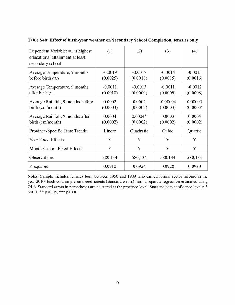
A similar analysis for the impact of in-utero temperature anomalies on educational

attainment did not reveal statistically significant patterns (see SI section and tables S4a-S4c),

potentially because the educational data available to us is limited to rather rough indicators of

high school and college completion.

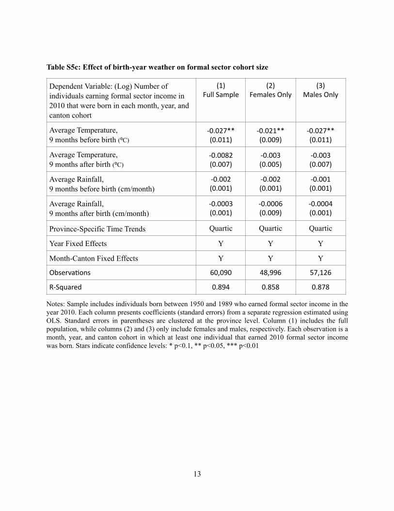
Cohort Size and Selection. The effect of weather anomalies on cohort size and on formal sector

cohort size represent the impacts on the probability of survival to adulthood and on the

probability of being employed in the formal sector. In addition to being of interest in themselves,

such effects can potentially bias the results of the earnings regressions, since they point to

selection effects into the sample (Almond and Currie, 2011).

Regression results indicate that cohorts that experience a 1⁰C increase in in-utero

temperature tend to be smaller by 2.6%. The effects are somewhat larger for males (3.0%) than

for women (2.2%) and are statistically significant (table S5a). Similar effects are found on the

sizes of formal sector workers, with male formal sector cohorts declining by 2.7% and female

formal sector cohorts declining by 2.1% (table S5c). The similar magnitudes of these impacts

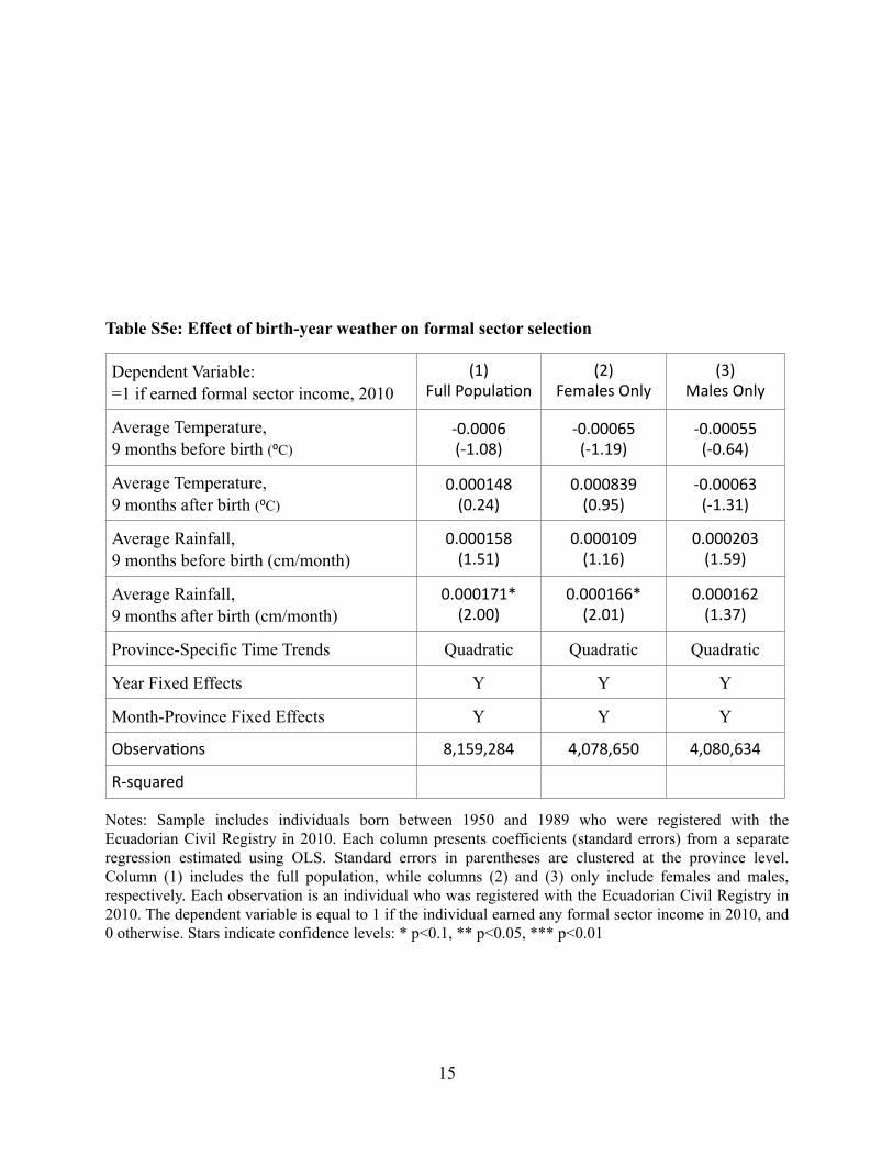
suggests the probably of being employed in the formal sector, conditional on survival to

adulthood, is unaffected by in-utero weather, and indeed, a regression of the ratio of formal

cohort and total cohort sizes (table S5d), or (at the individual level) of this probability on in-utero

temperature fails to find a statistically significant relationship (table S5e). We discuss the

implications of these results below.

8

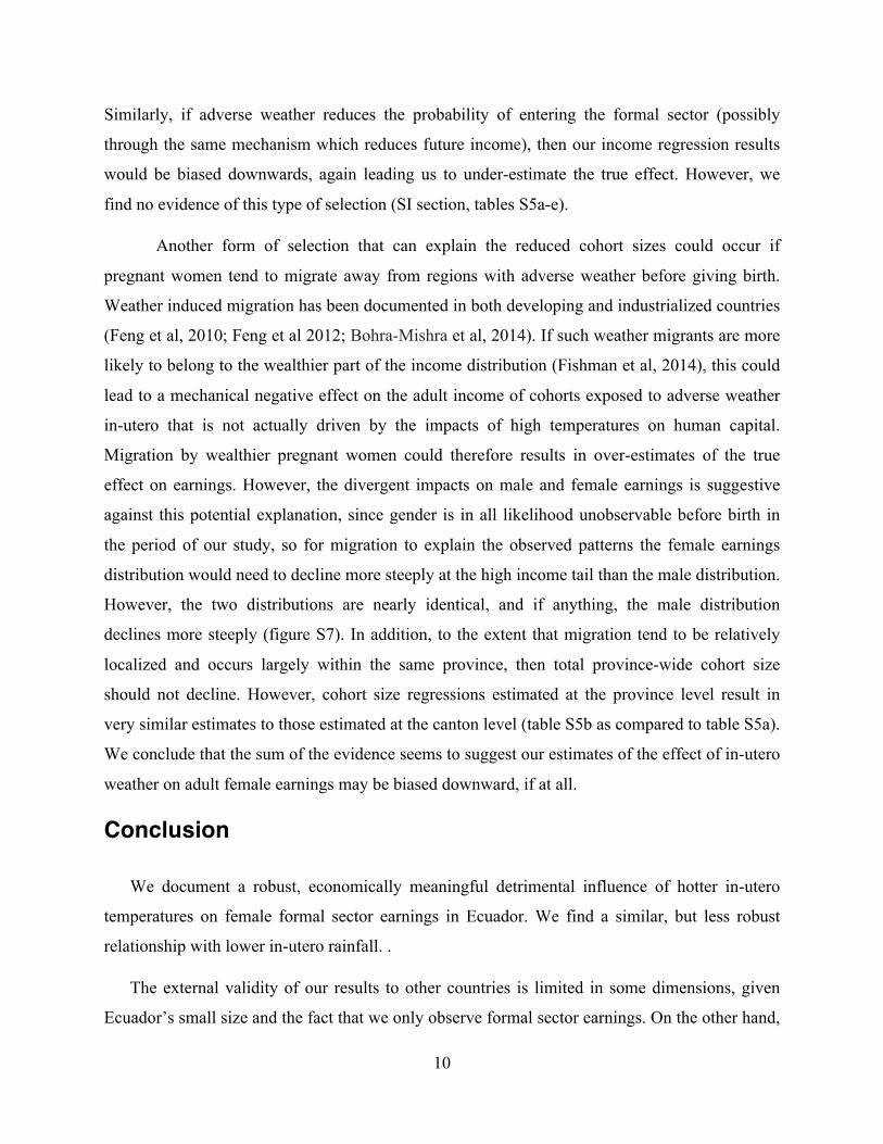
Falsification Tests. In order to examine the possibility that these results are driven by spurious

patterns in the earnings or weather data, we subjected them to a number of falsification tests. The

first test involved re-estimating regression (1) while replacing each individual’s in-utero weather

conditions with weather conditions that occurred at the location of birth up to 10 years before or

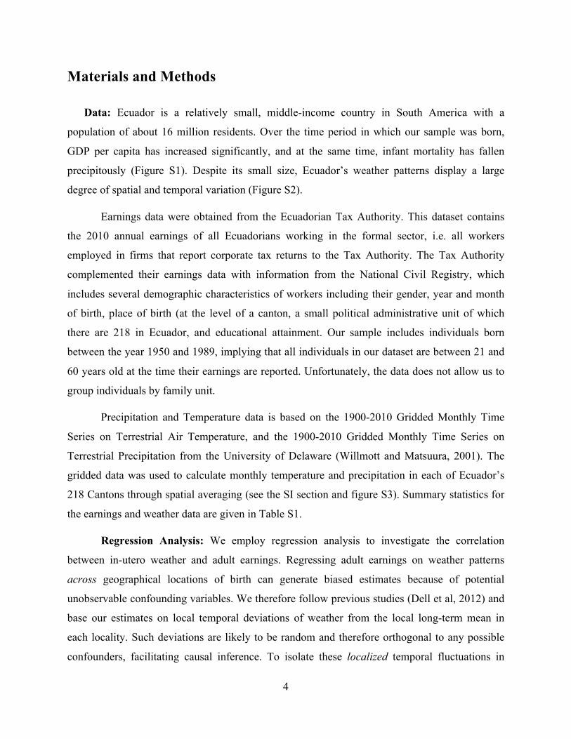
after birth. The resulting coefficient estimates are plotted in figure 3 against the “shift”, measured

in years. As would be expected, all “shifted” coefficients are smaller than the “true” coefficient,

plotted at zero, and other than the immediate lag and lead, are all statistically insignificant. The

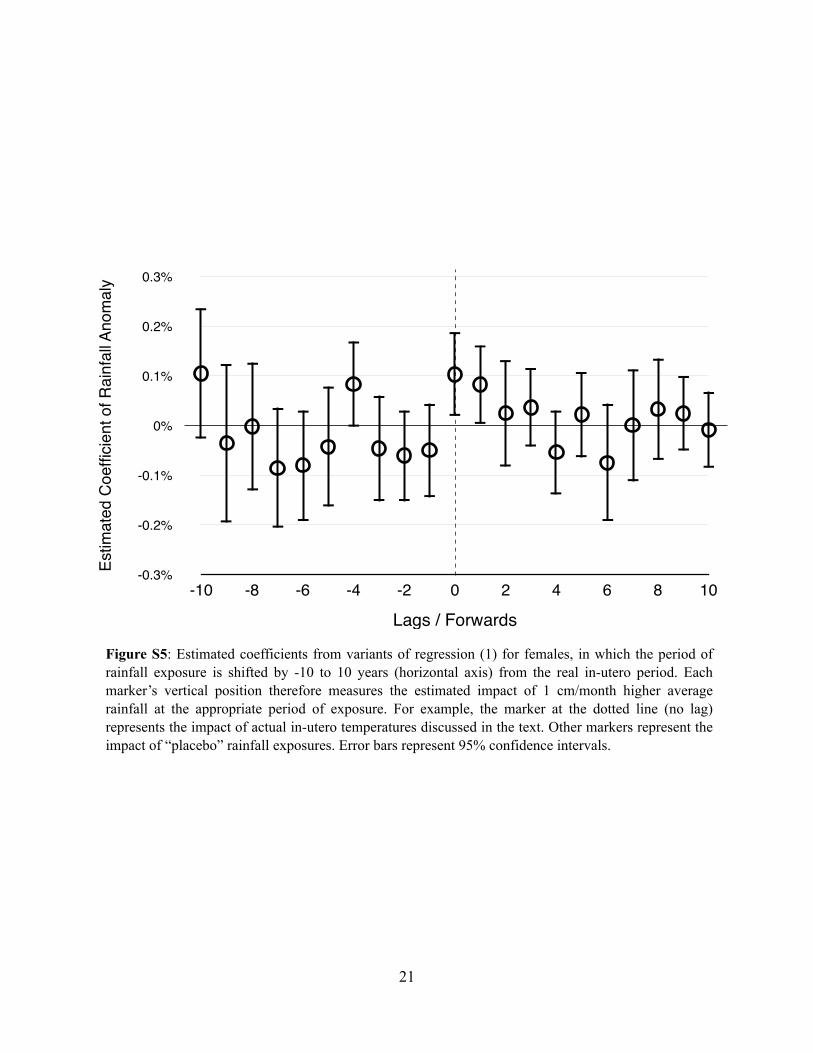
parallel results for rainfall are displayed in figure S5.

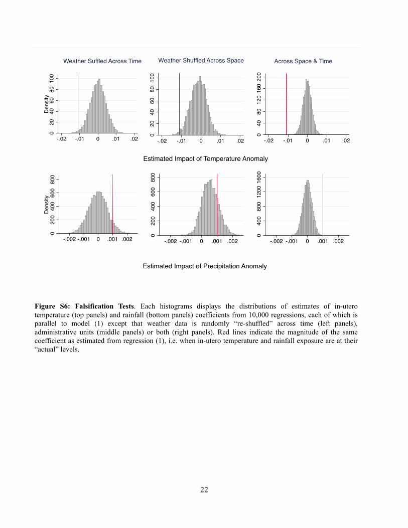
The second falsification test involved re-estimating equation (1) repeatedly on 10,000

“placebo” data sets in which all weather data was randomly re-shuffled between cohorts, either

across space, across time or both. As would be expected, histograms of all resulting “placebo”

coefficient estimates are centered around zero (figure S6), and the coefficient estimated using the

“real” data set lies at the extreme left end of the distribution (and is smaller than 99% of the

placebo estimates, whether re-shuffling occurred across space, time, or both). Together, these

tests indicate that the likelihood that the results found have occurred by chance is very low.

Discussion

The results of the “reduced-form” statistical analysis, while robust and causally

interpretable, do not allow us to isolate the mechanism(s) at play. However, the large literature

on the range of adverse impacts of high-temperature anomalies provides several possible

mechanisms, some of which, like increases in Malaria incidence (McCord, 2015) can be directly

relevant for Ecuador.

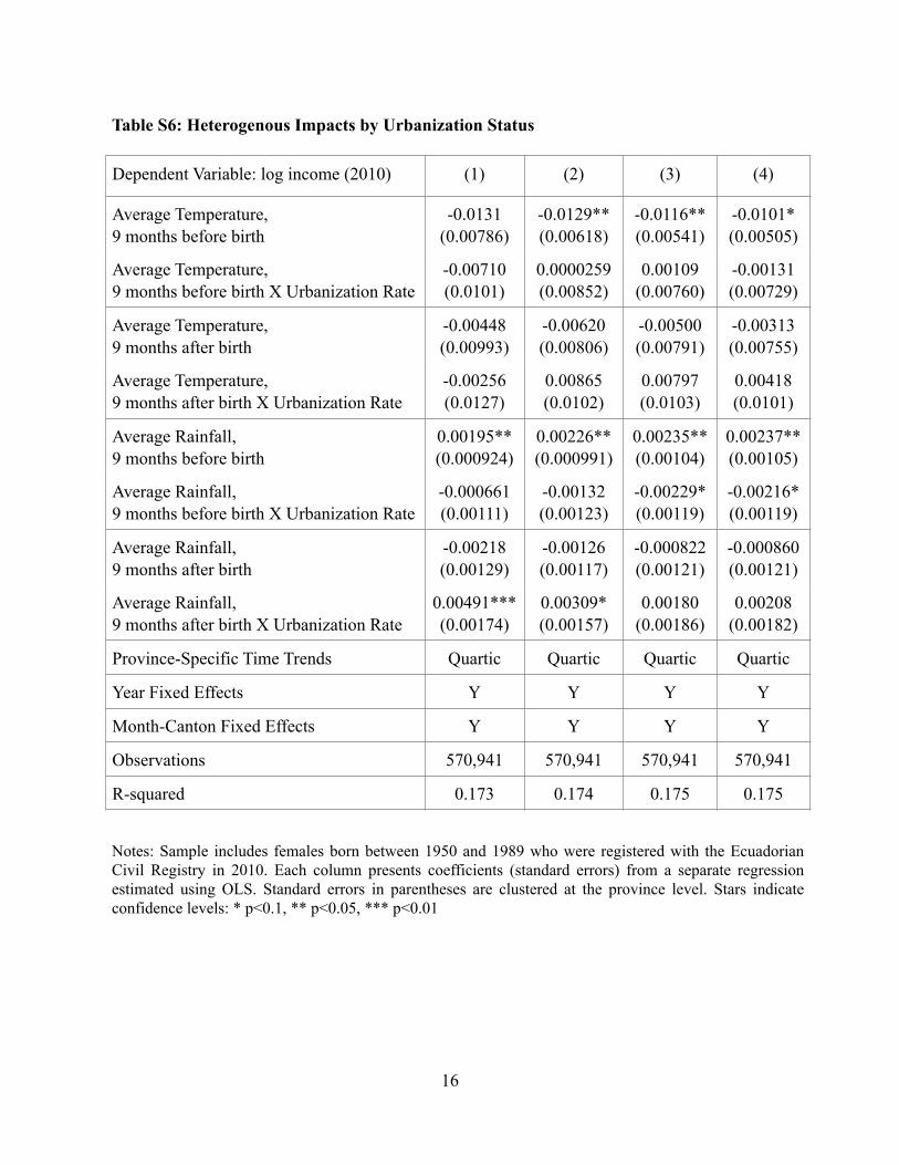
However, exploring heterogeneity in impacts across areas with varying rates of

urbanization can help shed light on the degree to which agricultural income declines may be

driving the observed temperature-earning relationship. A regression that included an interaction

between in-utero temperature anomalies and the degree of urbanization of each canton (in the

1990s) revealed that while precipitation anomalies tend to only occur in rural areas, in agreement

with the hypothesized central role of agricultural production shocks in channeling the impacts of

precipitation, no such effect was found for temperature anomalies, suggesting that non-

9

agricultural channels may have a central role in mediating the impacts of high temperatures (see

SI section and table S6 for details).

The appearance of larger and more statistically significant impacts of in-utero weather on

women relative to that on men is similar to the results of other studies that show that in poor

households, negative household shocks often tend to affect girls more than boys, presumably

because of gender bias in intra-household resource allocation in times of economic stress. For

example, Jayachandran (2005) find that infant mortality due to poor air quality was higher

amongst females than males. Maccini and Yang (2008) find that early life rainfall effects the

future incomes, health, and schooling of only females. Baird, Friedman and Schady (2011) find

that in developing countries, the infant mortality rate of females is much more sensitive to

economic shocks than the infant mortality rate of males

Our results, however, suggest that the impacts of high temperatures occur in-utero, when an

infant’s gender is likely to be unknown to parents. One possible interpretation is that corrective

investments can be made after birth to affected infants, and that these are less likely to be

provided to girls. A second possible explanation has to do with the well-documented higher

mortality rates of male fetuses subjected to in-utero stress in relation to females (Almond and

Mezumder, 2011), which is also consistent with the evidence presented above of reductions in

cohort sizes exposed to in-utero high temperature anomalies, that are larger for females than for

males. Fetal or infant mortality2 can remove the most vulnerable individuals from the adult

sample, leading to under-estimates of the true impact of high temperature in-utero. If mortality is

higher for males, this can also explain the lower impacts observed for males over females

(Almond and Currie, 2011).

Survival to adulthood is only one of possible selection effects that can potentially bias

regression estimates of adult earnings on in-utero weather and need to be carefully assessed. As

explained above, selection through survival to adulthood, which is well recognized in the fetal

origins literature, and for which we find some evidence, is likely to downward bias regression

estimates (Almond and Currie, 2011). This suggests the true effects are larger than our estimates. 2 Note that because our data from the civil registry only includes living people and not all births, we cannot distinguish between cohorts that are smaller because of additional fetal deaths, or additional infant, or even later in life mortality.

10

Similarly, if adverse weather reduces the probability of entering the formal sector (possibly

through the same mechanism which reduces future income), then our income regression results

would be biased downwards, again leading us to under-estimate the true effect. However, we

find no evidence of this type of selection (SI section, tables S5a-e).

Another form of selection that can explain the reduced cohort sizes could occur if

pregnant women tend to migrate away from regions with adverse weather before giving birth.

Weather induced migration has been documented in both developing and industrialized countries

(Feng et al, 2010; Feng et al 2012; Bohra-Mishra et al, 2014). If such weather migrants are more

likely to belong to the wealthier part of the income distribution (Fishman et al, 2014), this could

lead to a mechanical negative effect on the adult income of cohorts exposed to adverse weather

in-utero that is not actually driven by the impacts of high temperatures on human capital.

Migration by wealthier pregnant women could therefore results in over-estimates of the true

effect on earnings. However, the divergent impacts on male and female earnings is suggestive

against this potential explanation, since gender is in all likelihood unobservable before birth in

the period of our study, so for migration to explain the observed patterns the female earnings

distribution would need to decline more steeply at the high income tail than the male distribution.

However, the two distributions are nearly identical, and if anything, the male distribution

declines more steeply (figure S7). In addition, to the extent that migration tend to be relatively

localized and occurs largely within the same province, then total province-wide cohort size

should not decline. However, cohort size regressions estimated at the province level result in

very similar estimates to those estimated at the canton level (table S5b as compared to table S5a).

We conclude that the sum of the evidence seems to suggest our estimates of the effect of in-utero

weather on adult female earnings may be biased downward, if at all.

Conclusion

We document a robust, economically meaningful detrimental influence of hotter in-utero

temperatures on female formal sector earnings in Ecuador. We find a similar, but less robust

relationship with lower in-utero rainfall. .

The external validity of our results to other countries is limited in some dimensions, given

Ecuador’s small size and the fact that we only observe formal sector earnings. On the other hand,

11

that these impacts are occurring for formal sector workers in a middle-income country is striking.

Previous studies have mostly focused on samples that were dominated by rural farming

households. Additional studies of similar relationships would be important to conduct in other

contexts.

The size of the effect we find is economically meaningful. A simple extrapolation of our

estimates suggests that future warming may have additional economic impacts that have not been

sufficiently appreciated to date. In fact, our findings suggest that the warming that has already

occurred in Ecuador may have already resulted in large and to date unappreciated economic

losses. However, such extrapolations must be made with great caution, since, just as for short-

term impacts of high temperatures, the long-term impacts of an isolated temperature shock may

be quite different than that of a prolonged persistent change in temperature (Dell et al, 2013).

Nevertheless, our results may help improve our understanding of the mechanism driving the well

established cross-sectional inverse relationship between temperatures and economic income

(Nordhaus, 2006).

12

References

1. Dell, Melissa, Benjamin F. Jones, and Benjamin A. Olken. "What Do We Learn from the

Weather? The New Climate�Economy Literature."�Journal of Economic Literature�52.3

(2014): 740-798.

2. Deschenes, Olivier, and Michael Greenstone. "The economic impacts of climate change:

evidence from agricultural output and random fluctuations in weather." The American

Economic Review (2007): 354-385.

3. Lobell, David B., Wolfram Schlenker, and Justin Costa-Roberts. "Climate trends and

global crop production since 1980." Science 333.6042 (2011): 616-620.

4. Schlenker, Wolfram, and David B. Lobell. "Robust negative impacts of climate change

on African agriculture." Environmental Research Letters 5.1 (2010): 014010.

5. Guiteras, Raymond. "The impact of climate change on Indian agriculture." Manuscript,

Department of Economics, University of Maryland, College Park, Maryland (2009).

6. Fishman, Ram. "Climate change, rainfall variability, and adaptation through irrigation:

Evidence from Indian agriculture." Job Market Paper (2011).

7. Hsiang, Solomon M. "Temperatures and cyclones strongly associated with economic

production in the Caribbean and Central America." Proceedings of the National Academy

of Sciences 107.35 (2010): 15367-15372.

8. Dell, Melissa, Benjamin F. Jones, and Benjamin A. Olken. "Temperature shocks and

economic growth: Evidence from the last half century." American Economic Journal:

Macroeconomics 4.3 (2012): 66-95.

9. Sudarshan, Anant, and Meenu Tewari. The economic impacts of temperature on

industrial productivity: Evidence from indian manufacturing. Working Paper, 2013.

10. Zivin, Joshua Graff, and Matthew Neidell. "Temperature and the allocation of time:

Implications for climate change."�Journal of Labor Economics�32.1 (2014): 1-26.

13

11. Deryugina, Tatyana, and Solomon M. Hsiang.�Does the environment still matter? Daily

temperature and income in the United States. No. w20750. National Bureau of Economic

Research, 2014.

12. Burgess, Robin, et al. "Weather and death in India." Cambridge, United States:

Massachusetts Institute of Technology, Department of Economics. Manuscript (2011).

13. Patz, Jonathan A., et al. "Impact of regional climate change on human health."

Nature�438.7066 (2005): 310-317.

14. McMichael, Anthony J., Rosalie E. Woodruff, and Simon Hales. "Climate change and

human health: present and future risks."�The Lancet�367.9513 (2006): 859-869.

15. McMichael, Anthony J., Rosalie E. Woodruff, and Simon Hales. "Climate change and

human health: present and future risks."�The Lancet�367.9513 (2006): 859-869.

16. McCord, Gordon. �Malaria Ecology and Climate Change�. Forthcoming, European

Physics Journal.

17. Hsiang, Solomon M., Marshall Burke, and Edward Miguel. "Quantifying the influence of

climate on human conflict." Science 341.6151 (2013): 1235367.

18. Ranson, Matthew. "Crime, weather, and climate change."�Journal of environmental

economics and management�67.3 (2014): 274-302.

19. Blakeslee, David, and Ram Fishman. "Weather Shocks, Crime and Agriculture: Evidence

from India." Crime and Agriculture: Evidence from India (April 23, 2014) (2013).

20. Almond, Douglas, and Janet Currie. "Killing me softly: The fetal origins hypothesis."

The Journal of Economic Perspectives (2011): 153-172.

21. Maccini, Sharon L., and Dean Yang. �Under the weather: Health, schooling, and

economic consequences of early-life rainfall�. No. w14031. National Bureau of

Economic Research, 2008.

14

22. Aguilar, Arturo, and Marta Vicarelli. "El Nino and Mexican children: medium-term

effects of early-life weather shocks on cognitive and health outcomes." Cambridge,

United States: Harvard University, Department of Economics. Manuscript (2011).

23. Tiwari, Sailesh, Hanan G. Jacoby, and Emmanuel Skoufias. "Monsoon babies: rainfall

shocks and child nutrition in Nepal." World Bank Policy Research Working Paper 6395

(2013).

24. Deschênes, Olivier, Michael Greenstone, and Jonathan Guryan. "Climate change and

birth weight." The American Economic Review (2009): 211-217.

25. Willmott, C. J. and K. Matsuura (2001) Terrestrial Air Temperature: 1900-2010 Gridded

Monthly Time Series (V 3.01),

http://climate.geog.udel.edu/~climate/html_pages/Global2011/README.GlobalTsT2011

.html

26. Willmott, C. J. and K. Matsuura (2001) Terrestrial Precipitation: 1900-2010 Gridded

Monthly Time Series (V 3.01),

http://climate.geog.udel.edu/~climate/html_pages/Global2011/README.GlobalTsP2011

.html

27. Jayachandran, Seema. "Air quality and early-life mortality evidence from Indonesia’s

wildfires." Journal of Human Resources 44.4 (2009): 916-954.

28. Baird, Sarah, Jed Friedman, and Norbert Schady. "Aggregate income shocks and infant

mortality in the developing world." Review of Economics and Statistics 93.3 (2011):

847-856.

29. Almond, Douglas, and Bhashkar Mazumder. "Health capital and the prenatal

environment: the effect of Ramadan observance during pregnancy."�American Economic

Journal: Applied Economics�(2011): 56-85.

30. Feng, Shuaizhang, Alan B. Krueger, and Michael Oppenheimer. "Linkages among

climate change, crop yields and Mexico�US cross-border migration."Proceedings of the

National Academy of Sciences�107.32 (2010): 14257-14262.

15

31. Feng, Shuaizhang, Michael Oppenheimer, and Wolfram Schlenker.�Climate change, crop

yields, and internal migration in the United States. No. w17734. National Bureau of

Economic Research, 2012.

32. Bohra-Mishra, Pratikshya, Michael Oppenheimer, and Solomon M. Hsiang. "Nonlinear

permanent migration response to climatic variations but minimal response to

disasters."�Proceedings of the National Academy of Sciences(2014): 201317166.

33. Fishman, Ram, Meha Jain, and Avinash Kishore. "Groundwater Depletion, Adaptation

and Migration: Evidence from Gujarat, India." (2013).

34. Hsiang, Solomon M., and Amir S. Jina.�The causal effect of environmental catastrophe

on long-run economic growth: evidence from 6,700 cyclones. No. w20352. National

Bureau of Economic Research, 2014.

35. Nordhaus, William D. "Geography and macroeconomics: New data and new

findings."�Proceedings of the National Academy of Sciences of the United States of

America�103.10 (2006): 3510-3517.

!

! 1

Weather Anomalies (Precipitation, Temperature)

Stress (Physical &

Mental)

Disease Burden

In-Utero Stress

Human Capital

Earnings

Income Losses

(Agriculture)

Income Losses (Other)

Other

Reduced Consumption (Nutritional Deficiency)

(Household)

(Mother)

(Fetus)

(Adult)

Conflict

Figure 1: Possible channels of influence between weather anomalies in-utero on adult earnings. Observed variables appear in solid red boxes. Potential mediating variables are enclosed in dotted boxes and are unobserved in the data. These are classified into the economic (green boxes) and the physiological (purple boxes) channels. Numbers appearing next to each casual link (arrows) represent references to papers that demonstrate the associated impact empirically.

Figure 1: Possible channels of influence between weather anomalies in-utero on adult earnings. Observed variables appear in solid red boxes. Potential mediating variables are enclosed in dotted boxes and are unobserved in the data. These are classified into the economic (green boxes) and the physiological (purple boxes) channels. See text for references demonstrating some of these linkages.

!

! 2

Impa

ct o

n Ad

ult E

arni

ngs

(Fem

ale)

-3%

-2%

-1%

0%

1%

2%

3% Li

near

T.T

.

Qua

drat

ic T

.T.

Cub

ic T

.T.

Qua

rtic

T.T.

Temperature (C), Before Birth Temperature (C), After BirthPrecipitation (100mm), Before Birth Precipitation (100mm), After Birth

Figure 2: Regression estimates for the impact of average monthly temperature (red, degrees centigrade) and precipitation (blue, 100mm) anomalies in-utero (circles) on (Log) adult earnings. Error bars represent 95% confidence intervals. For comparison, dotted square markers represent parallel coefficients for the impacts of average monthly weather during the 9 months following birth (confidence intervals are not shown, but all coefficients are statistically insignificant). Estimates from models with localized time trends ranging from linear to quartic are presented from left to right.

!

! 3

Estim

ated

Coe

ffici

ent o

f Tem

pera

ture

Ano

mal

y

-2%

-1.5%

-1%

-0.5%

0%

0.5%

1%

1.5%

2%

Lags / Forwards-10 -8 -6 -4 -2 0 2 4 6 8 10

Figure 3: Estimated coefficients from variants of regression (1) for females, in which the period of temperature exposure is shifted by -10 to 10 years (horizontal axis) from the real in-utero period. Each marker’s vertical position therefore measures the estimated impact of one degree centigrade higher average temperatures at the appropriate period of exposure. For example, the marker at the dotted line (no lag) represents the impact of actual in-utero temperatures discussed in the text. Other markers represent the impact of “placebo” temperature exposures. Error bars represent 95% confidence intervals.

16

Supplementary Material

Data. The 1900-2010 Gridded Monthly Time Series on Terrestrial Air Temperature and

Precipitation from the University of Delaware (Willmott and Matsuura, 2001) compile weather

station data from several different sources, and interpolate monthly averages to a 0.5 degree by

0.5 degree latitude/longitude grid, with station nodes centered on the 0.25 degree. In order to

merge this gridded data with place of birth identifiers in the earnings data, weather values were

averaged across all grid cells falling within each canton, with weights proportional to the fraction

of area falling within the canton�s administrative boundaries (figure S3). Summary statistics for

the earnings and weather data are reported in Table S1.

Non-Parametric Estimation: To test for non-linear effects of in-utero weather, we

divided the range of observed precipitation and temperature observations into a series of

intervals and defined corresponding binary variables that indicate, for precipitation and

temperature separately, which of the intervals a given weather observation falls in. For

temperature, we divide the 7⁰C-29⁰C range into seven intervals of 3⁰C width each. For rainfall,

we divide the 0-30 cm/month range into 7 intervals, where the first 6 intervals are 4cm/month

wide each, and the 7th interval ranges from 24-30cm/month (we did this in lieu of adding an 8th

interval because only 8,319 females experienced a value between 28-30cm/month rainfall). We

then estimated a semi-parametric version of equation (1) in which the linear weather variables

are replaced with these 24 binary variables (7 each for temperature and rainfall, before and after

birth, with the indicator of the lowest intervals in each category omitted as a reference value),.

The estimated coefficients of these in-utero temperature and rainfall indicators are plotted in

figure S4. For both temperature and rainfall, we find that the pattern of the relationship is

approximately linear, justifying the use of a linear form in our main regressions. However, we

note that for rainfall, coefficients tend to be small and quite imprecise.

Are the Impacts Concentrated in Rural Regions? If the impacts of weather anomalies

are mostly occurring through their effect on agricultural production, one would expect them to be

concentrated in rural areas. To examine this hypothesis, we estimate a variant of model (1) that

also includes interaction terms between each of the four weather variables and a continuous

variable measuring the urbanization rate (the fraction of the population residing in urban

17

settlements) of each individual�s province of birth in 1990.3 These interaction terms measure the

degree to which impacts of weather anomalies are higher in more urbanized areas. The resulting

estimates are reported in Table S6.

Consistently with the hypothesis that rainfall anomalies operate mainly through their

impact on agricultural production, which is only a major source of income in rural areas, the

estimated interaction term of the in-utero rainfall is statistically significant and has a similar

magnitude (0.002) but opposite sign to the un-interacted rainfall coefficient (which measures the

impact of in-utero rainfall anomalies in completely rural areas). Thus, the more urbanized a

province is, the smaller is the effect of in-utero rainfall on the future earnings of those born there,

and the estimates point to a negligible effect of rainfall in completely urbanized locations.

The estimated interaction term between in-utero temperature and urbanization, in

contrast, is of very small magnitude (-0.001) in comparison to the un-interacted term (0.01).

Thus, we find no evidence to suggest that the effects of temperature differ between rural and

urban areas. 4 This can be suggestive of a temperature effect that is not primarily agricultural or

rural, which would not be inconsistent with the growing body evidence on the numerous non-

agricultural impacts of high temperature anomalies on economic productivity and welfare.

Impacts on Educational Attainment: Much of the literature on the impact of early life

weather shocks is focused on human capital accumulation, including indicators of educational

attainment. Unfortunately, our data only provides us with rather crude indicators of educational

attainment consisting of whether individuals had completed secondary school (84%) or college

(29%, Table S4a). In Tables S4b and S4c, we report estimates of regressions parallel to equation

(1) in which the dependent variable is a binary indicator of secondary education and higher

education, respectively. We find negative, but small and imprecise impact of in-utero

temperature exposure on either of these outcomes.

3 Urban populations rates are only available to us in one time period. The data was obtained from http://www.citypopulation.de/Ecuador-Cities.html 4 Note, however, that the confidence intervals of the interaction term are quite large. As a result, we are also unable to reject urban temperature effects that are substantially stronger or weaker than those in rural areas.

18

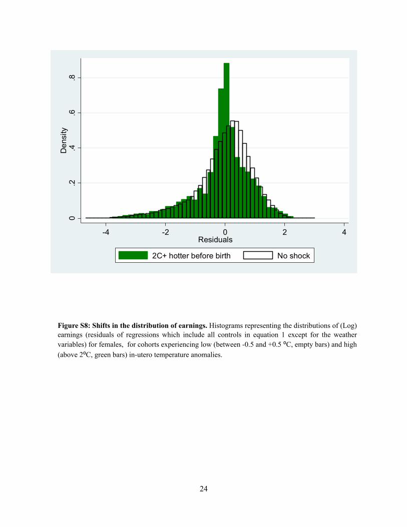
Impacts on the Distribution of Earnings.. In addition to estimating changes in mean

cohort earnings, we also examine the impact of temperatures anomalies on the distribution of

earnings. To do so, we calculate residuals from a regression of (log) earnings on the same fixed

effects and (quartic) time trends as in Equation (1), and then plot the residuals for two different

sub-samples: those females whose in-utero average temperature was between -0.5 and 0.5 of the

local average, and those whose in-utero average temperature was 2⁰C+ hotter than normal.5

Histograms of the two sets of residuals are overlaid in figure S8. Perhaps surprisingly, the

sample experiencing a 2⁰C+ hot temperature shock in-utero shows a significant shift in density

that mostly occurs in the right-central portion of the income distribution. Even though this is not

a conclusive indication, the pattern suggests that the effect does not seem to be primarily driven

by the low or high income tails of the earnings distribution.

Selection and Cohort Size: We begin by examining whether birth-cohort size is affected

by birth-year weather. To do this, we estimate a regression parallel to equation (1) except that the

unit of observation is a cohort rather than an individual and the dependent variable is the

logarithm of the cohort size, i.e. the number of individuals born in canton c, in month m of year

y. Results for the entire cohort, females only and males only are reported in columns 1-3 of table

S5a.,We find that a 1⁰C increase in in-utero temperature decreases the size of the birth cohort by

2.6%. The point estimate is larger for males (3.0%) than for females (2.2%). As discussed in the

text, changes in cohort size could be driven by survival to adulthood or by pre-birth migration by

the household. Lower likelihood of survival to adulthood is likely to downward bias the

estimated impacts on earnings, whereas selective migration by wealthier household may lead to

an upward bias.

In order to partially test whether this cohort size reduction is likely due to migration, we

run a similar regression, but re-define cohorts on the basis of province (a larger administrative

unit), rather than the canton, of birth. If most migration is relatively local in nature, for instance,

from rural areas to the nearest city, than most migration will be inter-provincial, so that,

provincial cohort sizes would be less affected by in-utero weather,. Results of the province level

5 These buckets are used after de-trending the weather data by taking the residuals from the regression of the weather data on the province specific time trends, and the fixed effects used in Equation (1).

19

regressions, reported in table S5b, are very similar to those reported in table S5a, suggesting

against inter-provincial migration as the main driver of the results. As discussed in the main text,

migration is also inconsistent with the diverging earnings results found for males and females..

Next, we test if in-utero weather affects one’s probability of entering the formal sector.

We do so in three different ways. In the first, we test if the count of the number of individuals

that earned formal sector income in 2010 in each cohort is affected by birth-year weather.

Results are reported in table S5c and indicate that hotter in-utero temperatures do tend to reduce

the formal sector cohort size. However, the magnitude of the effect is quite similar to the

magnitude of the reduction of the total birth cohort size reported in table S5a, suggesting against

additional reduction in the proportion of formal sector workers in a cohort. To test this directly,

we replace the dependent variable with the ratio of the number of formal sector cohort size to the

total cohort size, i.e. the percentage of individuals in each cohort working in the formal sector.

The results, reported in table S5d confirm that birth-year weather does not affect selection into

the formal sector, as all coefficients are very small and statistically insignificant. Finally, in the

last test for selection, we estimate whether the probability of entering the formal sector is

affected by early-life weather by estimating a regression parallel to equation (1) in which the

sample consists of all individuals in the civil registry, and the dependent variable is a binary

indicator of formal sector employment.6 We do not find any evidence for selection for either

males or females (table S5e).

Falsification Tests. In our first falsification test, we re-estimate Equation (1) while

replacing each individual’s in-utero weather exposure with weather occurring during �placebo�

9-month periods generated by displacing the actual in-utero period up to 10 years backwards and

forward in time. The resulting estimates are plotted in figure 3 (for temperature) and figure S5

(for precipitation) against the number of years by which weather was displaced in time, so that

the coefficients of the actual (non-placebo) regressions are plotted at the zero point on the

horizontal axis. We note that this falsification test may be too restrictive, in the sense that

�placebo� estimates could still be non-zero, for two reasons. First, serial correlation in weather

6 Note, due to computational restrictions, the regressions are estimated with quadratic province time-trends, rather than the standard quartic time trends.

20

can create significant correlations between the actual in-utero and placebo weather, and second,

it is not implausible that shocks occurring outside of the in-utero period may also affect future

earnings. For example, weather shocks occurring before conceptions could still impact

household welfare during pregnancy, and post-natal shocks could still be affecting adult

outcomes. Nevertheless, one would expect impacts to decline with the level of time

displacement. The results, displayed in figure 3, confirm this expectation. All placebo

temperature estimates are smaller than the actual one, and other than the first lag and lead, are all

statistically insignificant. Figure S5 shows a similar pattern for rainfall, i.e. that only the actual

and first lead coefficients statistically significant, with nearly all other point estimates being

small in magnitude and statistically insignificant...

In our second falsification test, we repeatedly and randomly “re-shuffle” the weather data

across time and space and re-estimate regression (1), in order to test the appropriateness of our

statistical model and the likelihood that our results are an artifact of chance or of a systematic

error in the data. We conduct three separate such “re-shufflings” (Hsiang and Jina 2014). In the

first, we randomly allocate to each birth cohort (individuals born in the same month, year, and

canton) the weather values from a different year, but in the same birth month and canton, and

then re-estimate Equation (1). We repeat this procedure 10,000 times and plot the distribution of

point-estimates (for the impact on in-utero temperature) in figure S6. We find that only 0.52% of

these estimates are larger in magnitude (and negative) than the actual coefficient, -0.0109,

indicated by the vertical line, implying that it is very unlikely that the estimates we found (table

2) arise by chance. In the second test, we “re-shuffle” weather across space. All individuals born

in the same birth cohort are now allocated birth-year weather from their year and month of birth,

but from a different canton. Given the granularity of the original weather data, as well as spatial

autocorrelation of weather data in general, adjacent cantons may have the same, or very similar

weather observations. This increases the likelihood that a birth cohort may be randomly assigned

weather data very similar or identical to its actual weather data, making this falsification test

highly conservative. Nevertheless, only 0.9% of the estimated coefficients on “in-utero”

temperature fall to the left of the actual coefficient. Finally, in the third test, we re-shuffle

weather across all cohorts, allocating to each cohort the weather in another, randomly chosen

birth month, year, and canton. None of the 10,000 bootstrapped estimates are larger in magnitude

than the actual estimate. These results indicate a very low likelihood that our results could have

21

arisen by chance. Also, as expected, the distributions of the �placebos� estimates are centered

around zero, providing a degree of validation to our model specification and the data sets we use.

The parallel results for rainfall are similar but less conclusive. Reshuffling across time, we find

that 6.27% of placebo estimates to be larger in magnitude (and positive) than the actual

coefficient, 0.001. Reshuffling across space, we find 20.86% of placebo estimates to be larger.

However, when reshuffling across both space and time, none of the placebo estimates are larger

than the actual estimate.

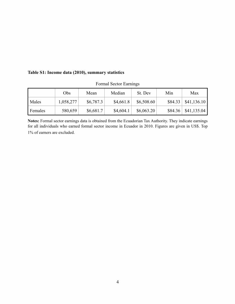
!!!!Table S1: Income data (2010), summary statistics

Notes: Formal sector earnings data is obtained from the Ecuadorian Tax Authority. They indicate earnings for all individuals who earned formal sector income in Ecuador in 2010. Figures are given in US$. Top 1% of earners are excluded. !

Formal Sector Earnings

Obs Mean Median St. Dev Min Max

Males 1,058,277 $6,787.3 $4,661.8 $6,508.60 $84.33 $41,136.10

Females 580,659 $6,681.7 $4,604.1 $6,063.20 $84.36 $41,135.04

! 4

Table S2: Average Monthly Weather !

Notes: Raw weather data is obtained from Willmott and Matsuura (2001), and is in the form of gridded monthly averages. Province averages are calculated by taking the spatially weighted average of all grids falling within a province. Annual averages are calculated by averaging the average monthly temperature for each month in a given year. !

ProvinceTemperature (⁰C) Rainfall (cm/month)

Mean Median St Dev Min Max Mean Median St Dev Min Max

Azuay 14.2 14.1 0.85 11.4 17.1 7.88 6.31 5.07 0.08 40.37

Bolivar 21.1 21.2 0.95 17.8 23.6 13.18 7.23 12.88 0.0 73.27

Carchi 17.9 17.9 0.73 15.5 20.6 13.93 13.50 4.65 4.39 35.91

Cañar 14.3 14.3 0.92 11.1 18.2 10.35 7.45 7.67 0.64 50.63

Chimborazo 11.6 11.7 0.82 8.7 13.8 7.73 6.50 5.13 0.98 51.51

Cotopaxi 13.5 13.6 0.81 10.7 16.1 12.01 10.05 7.75 0.26 51.51

El Oro 24.4 24.4 1.14 21.2 27.8 7.94 3.80 8.61 0.04 52.16

Esmeraldas 24.4 24.4 0.74 21.8 27.1 18.86 16.78 9.94 1.05 57.75

Guayas 24.6 24.6 1.22 20.2 27.4 10.93 3.62 13.53 0.02 79.99

Imbabura 18.1 18.0 0.92 14.6 23.4 9.73 9.21 5.56 0.47 34.82

Loja 20.4 20.4 1.00 17.2 23.9 7.74 4.53 7.66 0.13 50.07

Los Rios 24.3 24.4 1.00 20.6 27.0 15.75 8.06 16.43 0.0 88.65

Manabi 24.4 24.4 1.15 20.0 27.3 10.83 5.70 11.25 0.0 55.73

Morona Santiago

22.7 22.7 0.89 19.6 25.0 19.55 18.84 4.90 5.13 40.34

Napo 18.2 18.2 0.72 15.5 20.6 24.41 23.94 6.28 5.93 56.95

Orellana 25.3 25.3 0.81 22.3 27.9 26.04 24.73 7.40 5.26 48.23

Pastaza 25.6 25.7 0.78 22.6 27.8 29.27 29.04 6.23 8.55 55.21

Pichincha 15.2 15.2 0.70 12.1 17.5 14.36 12.69 8.83 1.03 43.30

Santa Elena 23.4 23.3 1.79 17.8 27.3 5.13 0.86 8.28 0.0 65.53

Santo Domingo

21.6 21.6 0.96 19.1 24.4 22.57 14.56 19.48 0.04 88.08

Sucumbios 23.9 23.9 0.83 21.1 26.7 21.48 21.34 6.50 4.02 53.68

Tungurahua 12.2 12.3 0.94 8.9 14.6 12.86 12.75 4.57 1.03 39.95

Zamora Chinchipe

20.9 21.0 0.92 17.8 24.1 12.30 11.11 4.86 0.84 43.14

! 5

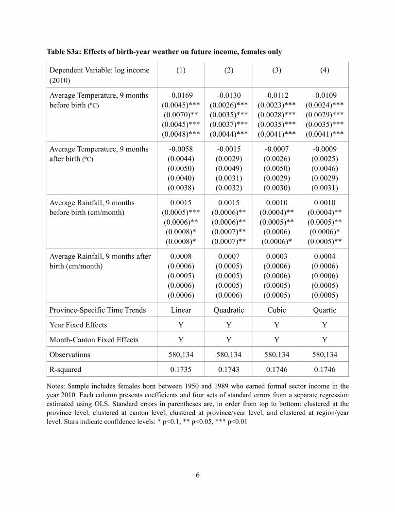
Table S3a: Effects of birth-year weather on future income, females only

Notes: Sample includes females born between 1950 and 1989 who earned formal sector income in the year 2010. Each column presents coefficients and four sets of standard errors from a separate regression estimated using OLS. Standard errors in parentheses are, in order from top to bottom: clustered at the province level, clustered at canton level, clustered at province/year level, and clustered at region/year level. Stars indicate confidence levels: * p<0.1, ** p<0.05, *** p<0.01 !!!

Dependent Variable: log income (2010)

(1) (2) (3) (4)

Average Temperature, 9 months before birth (⁰C)

-0.0169 (0.0045)*** (0.0070)** (0.0045)*** (0.0048)***

-0.0130 (0.0026)*** (0.0035)*** (0.0037)*** (0.0044)***

-0.0112 (0.0023)*** (0.0028)*** (0.0035)*** (0.0041)***

-0.0109 (0.0024)*** (0.0029)*** (0.0035)*** (0.0041)***

Average Temperature, 9 months after birth (⁰C)

-0.0058 (0.0044) (0.0050) (0.0040) (0.0038)

-0.0015 (0.0029) (0.0049) (0.0031) (0.0032)

-0.0007 (0.0026) (0.0050) (0.0029) (0.0030)

-0.0009 (0.0025) (0.0046) (0.0029) (0.0031)

Average Rainfall, 9 months before birth (cm/month)

0.0015 (0.0005)*** (0.0006)** (0.0008)* (0.0008)*

0.0015 (0.0006)** (0.0006)** (0.0007)** (0.0007)**

0.0010 (0.0004)** (0.0005)** (0.0006) (0.0006)*

0.0010 (0.0004)** (0.0005)** (0.0006)* (0.0005)**

Average Rainfall, 9 months after birth (cm/month)

0.0008 (0.0006) (0.0005) (0.0006) (0.0006)

0.0007 (0.0005) (0.0005) (0.0005) (0.0006)

0.0003 (0.0006) (0.0006) (0.0005) (0.0005)

0.0004 (0.0006) (0.0006) (0.0005) (0.0005)

Province-Specific Time Trends Linear Quadratic Cubic Quartic

Year Fixed Effects Y Y Y Y

Month-Canton Fixed Effects Y Y Y Y

Observations 580,134 580,134 580,134 580,134

R-squared 0.1735 0.1743 0.1746 0.1746

! 6

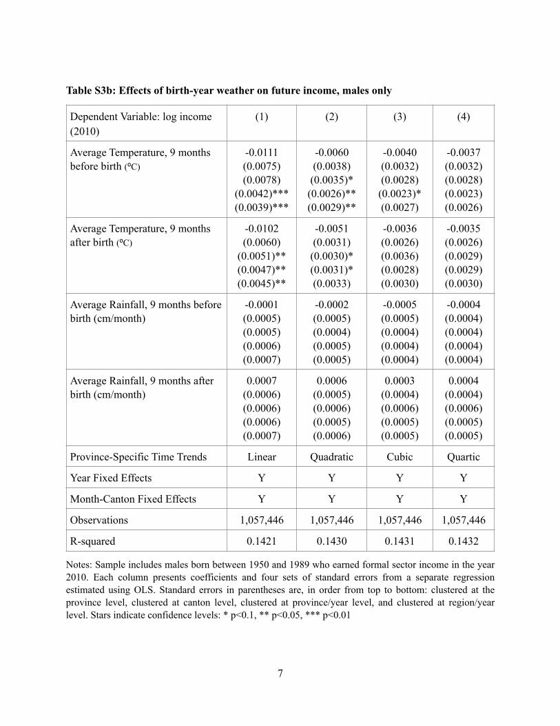
!Table S3b: Effects of birth-year weather on future income, males only

Notes: Sample includes males born between 1950 and 1989 who earned formal sector income in the year 2010. Each column presents coefficients and four sets of standard errors from a separate regression estimated using OLS. Standard errors in parentheses are, in order from top to bottom: clustered at the province level, clustered at canton level, clustered at province/year level, and clustered at region/year level. Stars indicate confidence levels: * p<0.1, ** p<0.05, *** p<0.01 !!

Dependent Variable: log income (2010)

(1) (2) (3) (4)


-0.0111 (0.0075) (0.0078)

(0.0042)*** (0.0039)***

-0.0060 (0.0038) (0.0035)* (0.0026)** (0.0029)**

-0.0040 (0.0032) (0.0028) (0.0023)* (0.0027)

-0.0037 (0.0032) (0.0028) (0.0023) (0.0026)


-0.0102 (0.0060)

(0.0051)** (0.0047)** (0.0045)**

-0.0051 (0.0031) (0.0030)* (0.0031)* (0.0033)

-0.0036 (0.0026) (0.0036) (0.0028) (0.0030)

-0.0035 (0.0026) (0.0029) (0.0029) (0.0030)


-0.0001 (0.0005) (0.0005) (0.0006) (0.0007)

-0.0002 (0.0005) (0.0004) (0.0005) (0.0005)

-0.0005 (0.0005) (0.0004) (0.0004) (0.0004)

-0.0004 (0.0004) (0.0004) (0.0004) (0.0004)


0.0007 (0.0006) (0.0006) (0.0006) (0.0007)

0.0006 (0.0005) (0.0006) (0.0005) (0.0006)

0.0003 (0.0004) (0.0006) (0.0005) (0.0005)

0.0004 (0.0004) (0.0006) (0.0005) (0.0005)




Observations 1,057,446 1,057,446 1,057,446 1,057,446

R-squared 0.1421 0.1430 0.1431 0.1432

! 7

Table S4a: Summary Statistics: Educational Attainment

Notes: Sample includes females born between 1950 and 1989 who earned formal sector income in the year 2010. Educational attainment data is obtained from the National Civil Registry and is merged with earnings data from the Ecuadorian tax authority. Data is from 2010.

!

Educational Attainment Percent completed, females

Percent completed, males

Average Income, females

Average Income, males

Less than Secondary School

16.25% 33.70% $3,225 $3,999

At least Secondary School

83.75% 66.30% $7,352 $8,204

At least College 29.43% 15.81% $9,832 $12,316

! 8

!Table S4b: Effect of birth-year weather on Secondary School Completion, females only

Notes: Sample includes females born between 1950 and 1989 who earned formal sector income in the year 2010. Each column presents coefficients (standard errors) from a separate regression estimated using OLS. Standard errors in parentheses are clustered at the province level. Stars indicate confidence levels: * p<0.1, ** p<0.05, *** p<0.01 !!!!!!!

Dependent Variable: =1 if highest educational attainment at least secondary school

(1) (2) (3) (4)


-0.0019 (0.0025)

-0.0017 (0.0018)

-0.0014 (0.0015)

-0.0015 (0.0016)


-0.0011 (0.0010)

-0.0013 (0.0009)

-0.0011 (0.0009)

-0.0012 (0.0008)


0.0002 (0.0003)

0.0002 (0.0003)

-0.00004 (0.0003)

0.00005 (0.0003)


0.0004 (0.0002)

0.0004* (0.0002)

0.0003 (0.0002)

0.0004 (0.0002)




Observations 580,134 580,134 580,134 580,134

R-squared 0.0910 0.0924 0.0928 0.0930

! 9

Table S4c: Effect of birth-year weather on College Completion, females only

Notes: Sample includes females born between 1950 and 1989 who earned formal sector income in the year 2010. Each column presents coefficients (standard errors) from a separate regression estimated using OLS. Standard errors in parentheses are clustered at the province level. Stars indicate confidence levels: * p<0.1, ** p<0.05, *** p<0.01

!!!!!!!!!!

Dependent Variable: =1 if highest educational attainment at least college

(1) (2) (3) (4)


-0.0059 (0.0043)

-0.0047* (0.0023)

-0.0034 (0.0023)

-0.0033 (0.0023)


-0.0046 (0.0028)

-0.0036** (0.0016)

-0.0020* (0.0011)

-0.0017* (0.0010)


0.0008** (0.0003)

0.0008*** (0.0003)

0.0006*** (0.0002)

0.0005** (0.0002)


0.0007* (0.0004)

0.0008** (0.0003)

0.0007** (0.0003)

0.0006** (0.0002)




Observations 580,134 580,134 580,134 580,134

R-squared 0.0798 0.0796 0.0805 0.0806

! 10

Table S5a: Effect of birth-year weather on birth cohort size, canton level

!Notes: Sample includes individuals born between 1950 and 1989 who were in the Ecuadorian civil registry in 2010. Each column presents coefficients (standard errors) from a separate regression estimated using OLS. Standard errors in parentheses are clustered at the province level. Column (1) includes the full population, while columns (2) and (3) only include females and males, respectively. Each observation is a month, year, and canton cohort in which at least one individual in the civil registry was born. Stars indicate confidence levels: * p<0.1, ** p<0.05, *** p<0.01

!!!!!!!!

Dependent Variable: (Log) number of individuals born in each month, year, and canton cohort

(1)%Full%Sample

(2)%Females%Only

(3)%Males%Only


50.0264**%(52.18)

50.0221*%(51.85)

50.0300**%(52.74)


50.0154%(51.40)

50.0162%(51.64)

50.0103%(50.91)


50.00109%(50.77)

50.0009%(50.67)

50.00134%(50.88)


50.00144%(51.13)

50.00155%(51.16)

50.0012%(51.06)

Province-Specific Time Trends Quartic% Quartic% Quartic%

Year Fixed Effects Y Y Y

Month-Canton Fixed Effects Y Y Y

ObservaBons 67,157 65,994 65,799

R5Squared 0.894 0.858% 0.878

! 11

Table S5b: Effect of birth-year weather on birth cohort size, province level

Notes: Sample includes individuals born between 1950 and 1989 who were in the Ecuadorian civil registry in 2010. Each column presents coefficients (standard errors) from a separate regression estimated using OLS. Standard errors in parentheses are clustered at the province level. Column (1) includes the full population, while columns (2) and (3) only include females and males, respectively. Each observation is a month, year, and province cohort in which at least one individual in the civil registry was born. Stars indicate confidence levels: * p<0.1, ** p<0.05, *** p<0.01

!!!!!!!!

Dependent Variable: (Log) Number of individuals born in each month, year, and province cohort

(1) Full Sample

(2) Females Only

(3) Males Only


-0.0188*** (0.005)

-0.0152** (0.007)

-0.0221*** (0.007)


0.00812 (0.007)

0.000833 (0.009)

0.0145** (0.006)


-0.00140* (0.001)

-0.00207*** (0.001)

-0.000982 (0.001)


-0.00261** (0.001)

-0.00214** (0.001)

-0.00295** (0.001)

Province-Specific Time Trends Quartic Quartic Quartic



Observations 11318 11312 11310

R-Squared 0.992 0.988 0.986

! 12

!Table S5c: Effect of birth-year weather on formal sector cohort size

Notes: Sample includes individuals born between 1950 and 1989 who earned formal sector income in the year 2010. Each column presents coefficients (standard errors) from a separate regression estimated using OLS. Standard errors in parentheses are clustered at the province level. Column (1) includes the full population, while columns (2) and (3) only include females and males, respectively. Each observation is a month, year, and canton cohort in which at least one individual that earned 2010 formal sector income was born. Stars indicate confidence levels: * p<0.1, ** p<0.05, *** p<0.01

!!!!!!!

Dependent Variable: (Log) Number of individuals earning formal sector income in 2010 that were born in each month, year, and canton cohort

(1)%Full%Sample

(2)%Females%Only

(3)%Males%Only


50.027**%(0.011)

50.021**%(0.009)

50.027**%(0.011)


50.0082%(0.007)

50.003%(0.005)

50.003%(0.007)


50.002%(0.001)

50.002%(0.001)

50.001%(0.001)


50.0003%(0.001)

50.0006%(0.009)

50.0004%(0.001)




ObservaBons 60,090 48,996 57,126

R5Squared 0.894 0.858% 0.878

! 13

!Table S5d: Effect of birth-year weather on formal sector cohort to birth cohort ratio

Notes: Sample includes individuals born between 1950 and 1989 who earned formal sector income in the year 2010. Each column presents coefficients (standard errors) from a separate regression estimated using OLS. Standard errors in parentheses are clustered at the province level. Column (1) includes the full population, while columns (2) and (3) only include females and males, respectively. Each observation is a month, year, and canton cohort in which at least one individual in the civil registry was born. Stars indicate confidence levels: * p<0.1, ** p<0.05, *** p<0.01

!!!!!!!!

Dependent Variable: Ratio of formal sector cohort size and birth cohort size

(1)%Full%Sample

(2)%Females%Only

(3)%Males%Only


50.0011(0.0013)

50.00005(0.00110)

50.002(0.0021)


50.0011(0.001)

50.0012(0.0013)

50.0017(0.0016)


0.0002(0.0002)

50.00002(0.0002)

0.0003(0.0003)


0.0003*(0.0002)

0.0001(0.0001)

0.0003(0.0002)




ObservaBons 67,157 65,994 65,799

R5Squared 0.285 0.194 0.256

! 14

!!!!!!Table S5e: Effect of birth-year weather on formal sector selection

Notes: Sample includes individuals born between 1950 and 1989 who were registered with the Ecuadorian Civil Registry in 2010. Each column presents coefficients (standard errors) from a separate regression estimated using OLS. Standard errors in parentheses are clustered at the province level. Column (1) includes the full population, while columns (2) and (3) only include females and males, respectively. Each observation is an individual who was registered with the Ecuadorian Civil Registry in 2010. The dependent variable is equal to 1 if the individual earned any formal sector income in 2010, and 0 otherwise. Stars indicate confidence levels: * p<0.1, ** p<0.05, *** p<0.01

!!

Dependent Variable: =1 if earned formal sector income, 2010

(1)%Full%PopulaBon

(2)%Females%Only

(3)%Males%Only


50.0006%(51.08)

50.00065%(51.19)

50.00055%(50.64)


0.000148%(0.24)

0.000839%(0.95)

50.00063%(51.31)


0.000158%(1.51)

0.000109%(1.16)

0.000203%(1.59)


0.000171*%(2.00)

0.000166*%(2.01)

0.000162%(1.37)

Province-Specific Time Trends Quadratic Quadratic Quadratic


Month-Province Fixed Effects Y Y Y

ObservaBons 8,159,284 4,078,650 4,080,634

R5squared

! 15

! 16

Dependent Variable: log income (2010) (1) (2) (3) (4)

Average Temperature, 9 months before birth

-0.0131 (0.00786)

-0.0129** (0.00618)

-0.0116**(0.00541)

-0.0101* (0.00505)

Average Temperature, 9 months before birth X Urbanization Rate

-0.00710 (0.0101)

0.0000259(0.00852)

0.00109(0.00760)

-0.00131 (0.00729)

Average Temperature, 9 months after birth

-0.00448 (0.00993)

-0.00620 (0.00806)

-0.00500 (0.00791)

-0.00313 (0.00755)

Average Temperature, 9 months after birth X Urbanization Rate

-0.00256 (0.0127)

0.00865(0.0102)

0.00797(0.0103)

0.00418(0.0101)

Average Rainfall, 9 months before birth

0.00195**(0.000924)

0.00226**(0.000991)

0.00235**(0.00104)

0.00237**(0.00105)

Average Rainfall, 9 months before birth X Urbanization Rate

-0.000661 (0.00111)

-0.00132 (0.00123)

-0.00229* (0.00119)

-0.00216* (0.00119)

Average Rainfall, 9 months after birth

-0.00218 (0.00129)

-0.00126 (0.00117)

-0.000822 (0.00121)

-0.000860 (0.00121)

Average Rainfall, 9 months after birth X Urbanization Rate

0.00491***(0.00174)

0.00309*(0.00157)

0.00180(0.00186)

0.00208(0.00182)

Province-Specific Time Trends Quartic Quartic Quartic Quartic



Observations 570,941 570,941 570,941 570,941

R-squared 0.173 0.174 0.175 0.175

Table S6: Heterogenous Impacts by Urbanization Status

Notes: Sample includes females born between 1950 and 1989 who were registered with the Ecuadorian Civil Registry in 2010. Each column presents coefficients (standard errors) from a separate regression estimated using OLS. Standard errors in parentheses are clustered at the province level. Stars indicate confidence levels: * p<0.1, ** p<0.05, *** p<0.01

!!

!

!!

! 17

!Figure S1: Economic growth and infant mortality rate during sample birth period. Bars (inner left axis) indicate the number of individuals in the sample that were born in each year. GDP per capita (center left axis, solid line), and infant mortality rate (outer left axis, dotted line) are also plotted (source: World Bank Development Indicators).

! 18

Figure S2: Time series of average annual temperature (⁰C, top panel) and precipitation (mm/month, bottom panel) for the provinces of Guayas, Bolivar, and Carchi between 1900 and 2010. Source: Authirs’ calculations based on Willmott and Matsuura (2001).

5010

015

020

025

0(m

ean)

rain

1900 1950 2000year

Guayas BolivarCarchi

1618

2022

2426

(mea

n) te

mp

1900 1950 2000year

Guayas BolivarCarchi

!!!!!!!!!!

! 19

Figure S3 : An overlay of average temperature (1950-1989) calculated from the gridded weather data of Willmott and Matsuura (2001) on a map of Ecuador’s administrative boundaries. The felt panel displays average temperatures from the raw gridded data and the right panel displays the result of spatial averaging of the gridded data within each administrative unit (canton).

! 20

!

!

!

!

-0.2

-0.16

-0.12

-0.08

-0.04

0

0.04

[7, 10) [10, 13) [13, 16) [16, 19) [19, 22) [22, 25) [25, 30)

Estim

ated

Coe

ffic

ient

(%

cha

nge

in in

com

e)

Temperature (�C)

-0.06

-0.04

-0.02

0

0.02

0.04

0.06

0.08

[1, 5) [5, 9) [9, 13) [13, 17) [17, 21) [21, 24) [24, 30)

Estim

ated

Coe

ffic

ient

(%

cha

nge

in in

com

e)

Rainfall (cm/month)

Figure S4: Semi-parametric estimates of the weather-earning relationship. The graph reports coefficients from a regression of log earnings (2010, females only) similar to model (1) except that linear expressions in rainfall and temperatures are replaced with a group of binary indicators for whether temperature and precipitation fall in specific rages indicated in the horizontal axis. Temperature coefficients are displayed in the top panel and rainfall coefficients are displayed in the bottom panel. Error bars indicate 95% confidence intervals.

!! !!

! 21

Figure S5: Estimated coefficients from variants of regression (1) for females, in which the period of rainfall exposure is shifted by -10 to 10 years (horizontal axis) from the real in-utero period. Each marker’s vertical position therefore measures the estimated impact of 1 cm/month higher average rainfall at the appropriate period of exposure. For example, the marker at the dotted line (no lag) represents the impact of actual in-utero temperatures discussed in the text. Other markers represent the impact of “placebo” rainfall exposures. Error bars represent 95% confidence intervals.

Estim

ated

Coe

ffici

ent o

f Rai

nfal

l Ano

mal

y

-0.3%

-0.2%

-0.1%

0%

0.1%

0.2%

0.3%

Lags / Forwards-10 -8 -6 -4 -2 0 2 4 6 8 10

! 22

020

4060

8010

0D

ensi

ty

-.02 -.01 0 .01 .02

Weather Suffled Across Time

020

4060

8010

0

-.02 -.01 0 .01 .02

Weather Shuffled Across Space

Estimated Impact of Temperature Anomaly

040

8012

016

020

0

-.02 -.01 0 .01 .02

Across Space & Time0

200

400

600

800

Den

sity

-.002 -.001 0 .001 .002 020

040

060

080

0

-.002 -.001 0 .001 .002

040

080

012

0016

00

-.002 -.001 0 .001 .002

Estimated Impact of Precipitation Anomaly

Estimated Impact of Temperature Anomaly

Figure S6: Falsification Tests. Each histograms displays the distributions of estimates of in-utero temperature (top panels) and rainfall (bottom panels) coefficients from 10,000 regressions, each of which is parallel to model (1) except that weather data is randomly “re-shuffled” across time (left panels), administrative units (middle panels) or both (right panels). Red lines indicate the magnitude of the same coefficient as estimated from regression (1), i.e. when in-utero temperature and rainfall exposure are at their “actual” levels.

! 23

0.2

.4.6

Density

-4 -2 0 2 4Residuals

Female Male

Figure S7: Histograms representing the distribution of (log) income residuals of males (transparent bars) and females (green shaded bars) after removing all controls in equation (1) other than weather variables.

! !!!

!!!

0.2

.4.6

.8D

ensi

ty

-4 -2 0 2 4Residuals

2C+ hotter before birth No shock

! 24

Figure S8: Shifts in the distribution of earnings. Histograms representing the distributions of (Log) earnings (residuals of regressions which include all controls in equation 1 except for the weather variables) for females, for cohorts experiencing low (between -0.5 and +0.5 ⁰C, empty bars) and high (above 2⁰C, green bars) in-utero temperature anomalies.

Documents

Human capital and growth - UNU-WIDER · 1957 E St. NW, Suite 502 Voice: (202) 994-5320 ... 2007; Lobell, Schlenker, and Costa-Roberts, 2011; Schlenker and Lobell, 2010; Guiteras,