NBER WORKING PAPER SERIES

HUMAN CAPITAL IN CHINA

Haizheng LiBarbara M. Fraumeni

Zhiqiang LiuXiaojun Wang

Working Paper 15500http://www.nber.org/papers/w15500

NATIONAL BUREAU OF ECONOMIC RESEARCH1050 Massachusetts Avenue

Cambridge, MA 02138November 2009

This project is funded by National Natural Science Foundation of China and Central University of Finance and Economics. This paper was drafted with excellent assistance form other project teammembers. The views expressed herein are those of the author(s) and do not necessarily reflect the viewsof the National Bureau of Economic Research.

NBER working papers are circulated for discussion and comment purposes. They have not been peer-reviewed or been subject to the review by the NBER Board of Directors that accompanies officialNBER publications.

© 2009 by Haizheng Li, Barbara M. Fraumeni, Zhiqiang Liu, and Xiaojun Wang. All rights reserved.Short sections of text, not to exceed two paragraphs, may be quoted without explicit permission providedthat full credit, including © notice, is given to the source.

Human Capital In ChinaHaizheng Li, Barbara M. Fraumeni, Zhiqiang Liu, and Xiaojun WangNBER Working Paper No. 15500November 2009JEL No. J24

ABSTRACT

In this paper we estimate China’s human capital stock from 1985 to 2007 based on the Jorgenson-Fraumenilifetime income approach. An individual’s human capital stock is equal to the discounted present valueof all future incomes he or she can generate. In our model, human capital accumulates through formaleducation as well as on-the-job training. The value of human capital is assumed to be zero upon reachingthe mandatory retirement ages.

China’s total real human capital increased from 26.98 billion yuan in 1985 (i.e., the base year) to 118.75billion yuan in 2007, implying an average annual growth rate of 6.78%. The annual growth rate increasedfrom 5.11% during 1985-1994 to 7.86% during 1995-2007. Per capita real human capital increasedfrom 28,044 yuan in 1985 to 106,462 yuan in 2007, implying an average annual growth rate of 6.25%.The annual growth rate also increased from 3.9% during 1985-1994 to 7.5% during 1995-2007. Therefore,although population growth contributed significantly to the total human capital accumulation before1994, per capita human capital growth was primary driving force after 1995. The substantial increasein educational attainment during 1985-2007 contributed significantly to the growth in total and percapita real human capital.

Haizheng LiSchool of EconomicsGeorgia Institute of TechnologyAtlanta, GA 30332haizheng.li@econ.gatech.edu

Barbara M. FraumeniMuskie School of Public ServiceUniversity of Southern MaineP.O. Box 9300Portland, ME 04104-9300and NBERbfraumeni@usm.maine.edu

Zhiqiang LiuSUNY BuffaloDepartment of Economics445 Fronczak HallBuffalo, NY 14260zqliu@buffalo.edu

Xiaojun WangUniversity of Hawaii at ManoaDepartment of Economics2424 Maile Way SSB 527Honolulu, HI 96822xiaojun@hawaii.edu

Introduction to

China Human Capital Index Project

“China Human Capital Measurement and Human Capital Index Project” is funded

by China National Natural Science Foundation and Central University of Finance and

Economics, conducted by China Center for Human Capital and Labor Market Research

(CHLR). The goal of this project is to establish China’s first set of systematic and

scientific measurements of human capital and quantify its distribution and dynamics. The

Indexes, once established, can be used to support empirical research as well as

government policy-making. In addition, the China human capital index we are

constructing is aimed at becoming an important part of the nascent international human

capital measurement system, and eventually being incorporated into the National Income

Accounting system.

This project is led by CHLR Director, Professor Haizheng Li. Professor Barbara

Fraumeni, who did the pioneer work in developing the popular Jorgenson-Fraumeni

method of calculating human capital stock, and all faculty members and graduate

students at the CHLR participated in the project.

This project requires a huge amount of data collection and processing. After one

year of daily effort, we have obtained China’s total human capital stock series from 1985

to 2007. We have also calculated disaggregated values by location (i.e. urban and rural)

and gender, and projected the series until 2020. Our results have seen rising attention

from international organizations such as the OECD, and we are actively looking for

opportunities of more international collaboration.

Contents

Executive Summary ............................................................................................................ I

I. Introduction..................................................................................................................... 3

II. Methodology ................................................................................................................. 6

II.1 Jorgenson-Fraumeni income-based approach ........................................................ 6

II.2 Cost approach ......................................................................................................... 9

II.3 Indicator approach ................................................................................................ 10

II.4 Attribute-based approach ..................................................................................... 11

II.5 Residual approach ................................................................................................ 12

III. Data ............................................................................................................................ 13

III.1 Population .......................................................................................................... 13

III.2 Obtaining parameter estimates of the Mincer equation ...................................... 19

III.3 Growth rates of real income and the discount rate ............................................. 28

III.4 Additional data imputations and assumptions for the Jorgenson- Fraumeni

estimates ............................................................................................................ 29

IV. Result discussions ...................................................................................................... 31

IV.1 Total human capital stock, GDP, and physical capital stock ............................. 31

IV.2 The trend of total human capital stock ............................................................... 38

IV.3 Per capita human capital .................................................................................... 46

IV.4 Divisia indexes ................................................................................................... 52

IV.5 Human capital in China 2008-2020: a projection .............................................. 54

V. Conclusions ................................................................................................................. 57

Reference List .................................................................................................................. 59

Acknowledgement……………………………………………………………………….64

Research Team Members

Principle Investigator

Haizheng Li Special-term Director, CHLR at CUFE

Associate Professor of Economics, Georgia Institute of

Technology

Members

Professors and Staff

Ake Blomqvist Professor, CHLR

Belton Fleisher Special-term Professor and Senior Fellow, CHLR

Professor of Economics, Ohio State University

Barbara Fraumeni Senior Fellow, CHLR

Associate Dean and Professor of Public Policy, Muskie

School of Public Service, University of Southern Maine

Zhiqiang Liu Special-term Professor, CHLR

Associate Professor of Economics, State University of New York

at Buffalo

Xiaojun Wang Special-term Professor, CHLR

Associate Professor of Economics, University of Hawaii at

Manoa

Kang-Hung Chang Assistant Professor, CHLR

Song Gao Assistant Professor, China Academy of Public Finance and

Public Policy, CUFE

Zhiyong Liu Instructor, Hunan University of Commerce

Ruiju Wang Executive Assistant to Director, CHLR

Hao Deng Graduate Coordinator, CHLR

Graduate Students

CHLR Yunling Liang (Ph.D.), Huajuan Chen, Yuhua Dong,

Mengxin Du, Jinquan Gong, Jingjing Jiang, Rui Jiang,

Qian Li, Sen Li, Chen Qiu, Xinping Tian, Mo Yang

Georgia Institute of

Technology

Yuxi Xiao

I

Executive Summary

In this project we estimate China’s human capital stock from 1985 to 2007 based

on the Jorgenson-Fraumeni lifetime income approach. An individual’s human capital

stock is equal to the discounted present value of all future incomes he or she can generate.

In our model, human capital accumulates through formal education as well as on-the-job

training. The value of human capital is assumed to be zero upon reaching the mandatory

retirement ages.

China’s total real human capital increased from 26.98 billion yuan in 1985 (i.e., the

base year) to 118.75 billion yuan in 2007, implying an average annual growth rate of

6.78%. The annual growth rate increased from 5.11% during 1985-1994 to 7.86% during

1995-2007. Per capita real human capital increased from 28,044 yuan in 1985 to 106,462

yuan in 2007, implying an average annual growth rate of 6.25%. The annual growth rate

also increased from 3.9% during 1985-1994 to 7.5% during 1995-2007. Therefore, although

population growth contributed significantly to the total human capital accumulation before

1994, per capita human capital growth was primary driving force after 1995. The

substantial increase in educational attainment during 1985-2007 contributed significantly to

the growth in total and per capita real human capital.

Since human capital accumulation was slower than GDP growth and physical

capital accumulation, the ratio of human capital to GDP fell from 30 in 1985 to 18 in

2007, the ratio of human capital to physical capital declined from 16 in 1985 to 11 in

2007. These values are not far away from those obtained in studies on other countries. An

important unanswered question is whether optimal values of human capital relative to

physical capital and GDP can be defined in relationship to sustainable economic growth.

In 2007, total male human capital was about twice that of total female human

capital, this gap is slightly larger than in 1985. However, female per capita human capital

is nearly 72% of male per capita human capital in 2007, indicating that most of the gap in

total human capital can be attributed to differences in population, returns to schooling and

work experience, and mandatory retirement age. Rural total human capital was greater

than that of urban in 1985, but urban overtook rural in the early 1990s, and by 2007 urban

total was about twice of rural total. Urban per capita human capital increased from 47,874

yuan in 1985 to 154,803 yuan in 2007, while rural per capita human capital increased

from 21,856 yuan to 66,164 yuan. The rural-urban gap increased by about 3 percentage

points (i.e., the rural-urban per capita human capital ratio was 45.7% in 1985 and 42.7%

in 2007).

II

In our projection from 2007 to 2020, total human capital will grow at a much

slower annual rate of 0.61%. This is mainly because we assume future parameters and

values will remain the same as their 2007 values. Urban total human capital will continue

to rise, while rural total human capital will slowly decline, mainly due to continued

migration and urbanization. Per capita human capita, however, will remain constant in

the rural area and will grow slowly in the urban area.

3

I. Introduction

Since the concept of human capital was introduced to modern economic analysis

by Schultz (1961) and Becker (1964), it has been widely used in academic studies and

policy analysis. Human capital is probably “the most important and most original

development in the economics of education” in the second part of the 20th century

(Coleman, 1990, page 304). The latest definition of human capital from the Organization

for Economic Co-operation and Development (OECD) is “The knowledge, skills,

competencies and attributes embodied in individuals that facilitate the creation of

personal, social and economic well-being” (OECD, 2001, page 18). In most countries,

human capital accounts for more than 60% of the nation’s wealth, which includes natural

resources, physical capital and human capital (World Bank, 1997).

It is generally believed that human capital is an important source of economic

growth and innovation, an important factor for sustainable development, and for reducing

poverty and inequality (see, for example, Stroombergen et al., 2002, and Keeley, 2007).

For example, the detailed analysis of human capital accounts for Canada, New Zealand,

Norway, Sweden, and the United States unanimously shows that human capital is a

leading source of economic growth.1

In China, since the start of economic reforms, the economy has grown at a dramatic

rate. It is believed that human capital has played a significant role in the Chinese

economic miracle (see, for example, Fleisher and Chen, 1997, and Démurger, 2001).

Additionally, studies show that human capital also has an important effect on productivity

growth and on reducing regional inequality in China (Fleisher, Li and Zhao, 2009).

Despite the important role of human capital in the Chinese economy, however,

until now, there has been almost no comprehensive measurement of the total stock of

human capital in China. Human capital measures for China are central to any

understanding of the global importance of human capital for a number of reasons. First,

China is the most populous country in the world. It is important to understand the

dynamics of human capital caused by demographic changes (for example, due to

one-child policy, migration, and urbanization) and by the rapid expansion of education

during the course of economic development. Second, such measures would allow for

better assessment of the contribution of human capital to growth, development, and social

well-being in empirical and theoretical research. Construction of human capital measures

1 These include Jorgenson-Fraumeni (J-F) accounts for Canada (Gu and Ambrose 2008), New Zealand (Le, Gibson, and Oxley 2005), Norway (Greaker and Liu 2008), Sweden (Alroth 1997), and the United States (Jorgenson and Fraumeni 1989, 1992a, 1992b, and Christian 2009).

4

is an important step in assessing the contribution of human capital to economic growth.

Currently, only partial measurement of human capital, such as education characteristics,

has been used in such studies.

Additional benefits from human capital measures include the provision of useful

information for policy makers, such as assessing how education policies of central and

local governments affect the accumulation of human capital. This is especially important,

given the long-term nature of human capital investment. For example, since the early

1980s, there has been a remarkable increase in the educational attainment of the Chinese

population. In 1982 the largest population mass was concentrated in the “no schooling”

category (Figure III.1.4). By 2007 the largest population mass was concentrated in the

“junior middle” school category (Figure III.1.7). Developing comprehensive measures of

human capital in China provides the necessary early work for constructing China’s

human capital account and for eventually incorporating human capital into the national

accounting so that China can join the international OECD initiative. It would facilitate

international comparison of human capital accumulation and growth across nations.

There is an ongoing international effort in developed countries to measure a

nation’s total human capital stock and to develop national human capital accounts. For

example, the United States formed the Committee on National Statistics’ Panel to Study

the Design of Nonmarket Accounts (Abraham 2005, and Christian 2009); in early 2008,

Statistics Canada set up a program “Human Development and its Contribution to the

Wealth Accounts in Canada” (Gu and Wong 2008); Australian Bureau of Statistics (Wei

2008), Statistics Norway (Greaker and Liu 2008) and New Zealand (Le, Gibson, and

Oxley 2005), have also established similar research program on the measurement of

human capital. In addition, seventeen countries: Australia, Canada, Denmark, France,

Italy, Japan, Korea, Mexico, Netherlands, Norway, New Zealand, Poland, Spain, the

United Kingdom, the United States, Romania, and Russia, and two international

organizations Eurostat and the International Labour Organization, have agreed to join the

OECD consortium to develop human capital accounts. A researcher from Statistics

Norway, Gang Liu, is at the OECD as of October 1, 2009 for nine months to coordinate

this effort. The work of this consortium will facilitate cross-country comparisons. In

addition, the Lisbon Council European Human Capital Index has been constructed for the

13 European Union (EU) states and 12 Central and Eastern European states (See Ederer

2006 and Ederer et. al. 2007). Developed countries have obviously realized the

importance of monitoring human capital accumulation, while most developing countries

have yet to start such projects, including China.

Until now, there has been no systematic effort to construct comprehensive

measures of the total human capital stock in China. There are a few studies on human

5

capital measurement published in Chinese journals. For example, Zhang (2000) and Qian

and Liu (2004) calculated China’s human capital stock based on total investment

(cost-side); others, such as Zhu and Xu (2007), Wang and Xiang (2006), estimated

human capital from the income side. Zhou (2005) and Yue (2008) used some weighted

average of human capital attributes to construct a measurement. In most cases, these

studies partially measure human capital based on some education characteristics such as

average education, for example, Cai (1999), Hu (2002), Zhou (2004), Hou (2000), Hu

(2005), etc.

While the above studies did contribute to the understanding of human capital in

China, there are major limitations. First, there has been no comprehensive and systematic

measurement of the total human capital stock in China from the 1980s up to date,

especially on the changes of human capital in rural and urban areas and for males and

females respectively. Second, the methodology used has been limited by data availability,

feasibility of parameter estimation, and some technical treatment difficulties. Thus, there

has no exact implementation of internationally recognized methods to China’s data for

human capital estimation.

We attempt to construct a comprehensive measurement of human capital in China

by applying the methods used in other countries after modifying them to fit China’s

special cases. We estimate total human capital at the national level, for male and female,

for urban and rural areas from 1985 to 2007. Our estimates include nominal values, real

values, indexes, and quantity measures. We mostly adopted the Jorgensen- Fraumeni (J-F)

lifetime income based approach, which has been widely used in other countries.

In addition to a full-implementation of the J-F approach to China’s data to estimate

the human capital series, another contribution of this study is that we combine

micro-level survey data in human capital estimation to mitigate the lack of earnings data

in China. In particular, we apply the Mincer equation to estimate earnings by using

various available household survey data. Thus, it is possible to integrate the changes of

returns to education and experience (on-the-job-training) into our estimates during the

course of economic transition.

Moreover, by separating the calculation of human capital for urban and rural areas,

we are able to capture the changes caused by rapid urbanization as well as by the large

scale rural-urban migration since the start of economic reform in China. This framework

is not only important for any transitional economy because of its changing economic

structure and migration, it can also at least partially measure the effect of another type of

human capital investment—migration, which helps realize higher value of one’s human

capital.

6

The rest of this report is arranged as follows. Section II discusses methodology for

human capital measurement. Section III describes our data and data treatments. The

estimated results of human capital are reported in Section IV. Section V concludes. All

data and technical details are reported in appendixes which can be obtained online from

the NBER web site.

II. Methodology

In general, human capital can be produced by education and training (child bearing

and rearing are investments that increase future human capital), as well as by job turnover

and migration that help to realize the potential value of human capital. Like physical

capital stock, the human capital can be valued using two methods: i) it can be valued as

the sum of investment, minus depreciation, added over time to the initial stock; ii) it can

be valued as the net present value of the income flow it will be able to produce over an

assumed lifetime. The first method, the perpetual inventory method, is used in the cost

approach; while the second method is the income-based approach (this method is used to

estimate the value of most natural resources). When human capital is measured using the

perpetual inventory approach, only costs or expenditures are included in investment.

When physical capital is measured, investments are valued at their purchase price which

is not generally available for human capital.

There are several measures of human capital commonly adopted by researchers:

(1) The lifetime income approach of Jorgenson and Fraumeni (1989, 1992a,

1992b);

(2) The cost approach of Kendrick (1976);

(3) The indicator approach;

(4) Laroche and Merette (2000) construct indexes with either relative wage

weights or relative lifetime income weights;

(5) The Lisbon Council’s approach (2006) is described as an example of the

indicator approach;

(6) The World Bank residual approach (2006).

The approach of Jorgenson-Fraumeni is discussed further next.

II.1 Jorgenson-Fraumeni income-based approach

The Jorgenson and Fraumeni (J-F) income-based approach is the most widely used

method in estimating human capital stock, and has been adopted by a number of countries

7

in constructing human capital accounts (see footnote 1 for examples). The advantages of

this approach are that it has a sound theoretical foundation and that the data and

parameters are relatively easier to obtain than they are for other approaches.

When estimating lifetime income to calculate human capital, an important issue is

that income (or implicit income) can be generated from both market and non-market

activities. Market activities of individuals produce goods and services, foster innovation

and growth through managerial and creative activities, and generate income that allows

for the acquisition of market goods and services. Nonmarket activities of individuals

include household production, e.g., cooking, cleaning, and care-giving. Investment is

generated from both market and nonmarket activities. Because household production

activities are difficult to quantify and value and require time-use estimates, we have opted

to exclude them in this first approximation to estimating China’s human capital.2 The J-F

approach imputes expected future lifetime incomes based on survival, enrollment, and

employment probabilities. Expected future wages and incomes are estimated from the

currently observed wages and incomes of the cross section of individuals who are older

than a given cohort at the time of observation. Future incomes are augmented with a

projected labor income growth rate and discounted to the present with a constant interest rate.

Estimation is conducted in a backward recursive fashion, from those aged 75, 74, 73, and so

forth to those aged 0.3

With the J-F income-based approach, we first need data or estimates of individual’s

annual market labor income per capita. Then lifetime incomes are calculated by a

backward recursion, starting from the oldest cohorts in the population. The life cycle is

divided into five stages, and the equations used for calculating the lifetime expected

incomes are as follows.

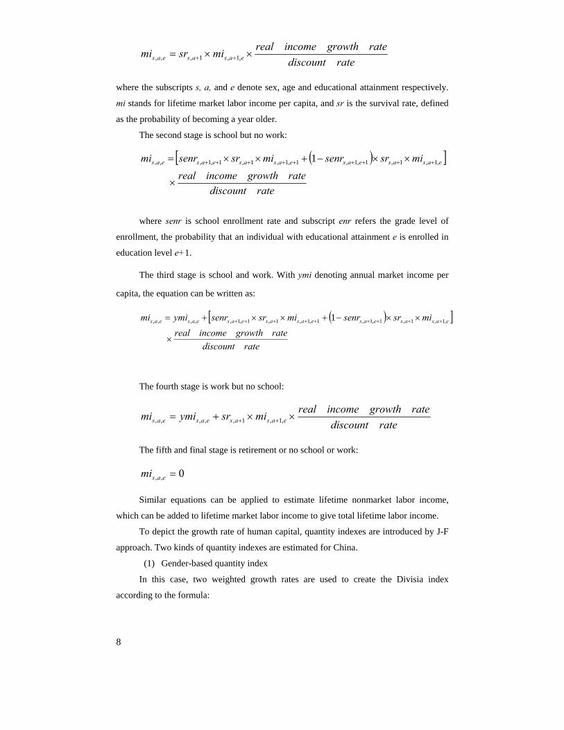
The first stage is no school and no work:

2 Among the most recent human capital estimates, i.e., Gu and Ambrose (2008), Greaker and Liu (2008) and Christian (2009), only Christian, for the United States, includes a full set of nonmarket activities and estimates human capital for those too young to go to school or to perform market work. 3 The J-F inclusion of nonmarket lifetime income and expected lifetime income for youngsters produces human capital estimates that are notably higher than those in the studies mentioned above who have adopted the J-F methodology.

8

ratediscountrategrowthincomerealmisrmi easaseas ××= ++ ,1,1,,,

where the subscripts s, a, and e denote sex, age and educational attainment respectively.

mi stands for lifetime market labor income per capita, and sr is the survival rate, defined

as the probability of becoming a year older.

The second stage is school but no work:

( )[ ]

ratediscountrategrowthincomereal

misrsenrmisrsenrmi easaseaseasaseaseas

×

××−+××= +++++++++ ,1,1,1,1,1,1,1,1,1,,, 1

where senr is school enrollment rate and subscript enr refers the grade level of

enrollment, the probability that an individual with educational attainment e is enrolled in

education level e+1.

The third stage is school and work. With ymi denoting annual market income per

capita, the equation can be written as:

( )[ ]

ratediscountrategrowthincomereal

misrsenrmisrsenrymimi easaseaseasaseaseaseas

×

××−+××+= +++++++++ ,1,1,1,1,1,1,1,1,1,,,,, 1

The fourth stage is work but no school:

ratediscountrategrowthincomerealmisrymimi easaseaseas ××+= ++ ,1,1,,,,,

The fifth and final stage is retirement or no school or work:

0,, =easmi

Similar equations can be applied to estimate lifetime nonmarket labor income,

which can be added to lifetime market labor income to give total lifetime labor income.

To depict the growth rate of human capital, quantity indexes are introduced by J-F

approach. Two kinds of quantity indexes are estimated for China.

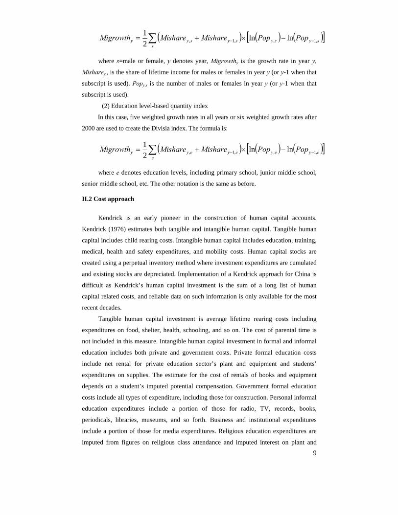
(1) Gender-based quantity index

In this case, two weighted growth rates are used to create the Divisia index

according to the formula:

9

( ) ( ) ( )[ ]∑ −− −×+=s

sysysysyy PopPopMishareMishareMigrowth ,1,,1, lnln21

where s=male or female, y denotes year, Migrowthy is the growth rate in year y,

Misharey,s is the share of lifetime income for males or females in year y (or y-1 when that

subscript is used). Popy,s is the number of males or females in year y (or y-1 when that

subscript is used).

(2) Education level-based quantity index

In this case, five weighted growth rates in all years or six weighted growth rates after

2000 are used to create the Divisia index. The formula is:

( ) ( ) ( )[ ]∑ −− −×+=e

eyeyeyeyy PopPopMishareMishareMigrowth ,1,,1, lnln21

where e denotes education levels, including primary school, junior middle school,

senior middle school, etc. The other notation is the same as before.

II.2 Cost approach

Kendrick is an early pioneer in the construction of human capital accounts.

Kendrick (1976) estimates both tangible and intangible human capital. Tangible human

capital includes child rearing costs. Intangible human capital includes education, training,

medical, health and safety expenditures, and mobility costs. Human capital stocks are

created using a perpetual inventory method where investment expenditures are cumulated

and existing stocks are depreciated. Implementation of a Kendrick approach for China is

difficult as Kendrick’s human capital investment is the sum of a long list of human

capital related costs, and reliable data on such information is only available for the most

recent decades.

Tangible human capital investment is average lifetime rearing costs including

expenditures on food, shelter, health, schooling, and so on. The cost of parental time is

not included in this measure. Intangible human capital investment in formal and informal

education includes both private and government costs. Private formal education costs

include net rental for private education sector’s plant and equipment and students’

expenditures on supplies. The estimate for the cost of rentals of books and equipment

depends on a student’s imputed potential compensation. Government formal education

costs include all types of expenditure, including those for construction. Personal informal

education expenditures include a portion of those for radio, TV, records, books,

periodicals, libraries, museums, and so forth. Business and institutional expenditures

include a portion of those for media expenditures. Religious education expenditures are

imputed from figures on religious class attendance and imputed interest on plant and

10

equipment of religious organizations. Government expenditures include those for library,

recreation costs and military expenditures.

Intangible human capital investment in training values initial nonproductive time

and nonwage costs and includes explicit training expenditures. Both specific and general

training is captured, as well as military training. A substantial fraction of medical, health

and safety expenditures, which are split between investment and preventive expenditures,

are by governments. Annual rental costs for plant and equipment are imputed when not

available.

Kendrick considers his human capital mobility investment estimates to be tentative.

These include unemployment, job-search, hiring, and moving costs, for both residents

and immigrants. Depreciation is estimated using the depreciation methodology most

widely used at the time of his research: A double declining balance formula with a switch

to a straight-line method. Lifetimes in these formulas are assumed to be the reciprocal of

the percentage of persons in the group.

Kendrick nominal human capital is about five times Gross Domestic Product.

However, Jorgenson-Fraumeni human capital is substantially larger than Kendrick human

capital.4 The Kendrick approach covers detailed aspects of human capital formation from

the cost side and provides a very complete menu for sum up all related cost to estimate

the value of human capital. Yet, the data requirement is enormous, for example, we may

need to get government statistics ninety years back to do the calculation. This is

impossible, given the People’s Republic of China is only 60 years old in 2009.

Additionally, it lacks guideline for many technique treatments, such as for the split of

health expenses between investment and preventative costs. Therefore, we do not adopt it

here for our calculation.

II.3 Indicator approach

An example of an indicator approach is the Human Capital Index of the Lisbon

Council. It is a human capital input cost, or cost of creation approach. This index has

been constructed for the 13 European Union (EU) states and 12 Central and Eastern

European states as previously noted.5 The Human Capital Endowment measure is an

input to two of the other three components of the overall European Human Capital Index.

The Human Capital Endowment measure sums up expenditures on formal education and

4 See table 37 of Jorgenson-Fraumeni (1989). 5 See Ederer (2006) and Ederer et. al.(2007). The 2006 paper states that the index was developed by the German think tank Deutschland Denken. In addition the paper states that the paper is part of a research project undertaken by several individuals in the think tank and with the institutional support of Zeppelin University.

11

the opportunity cost of parental education, adult education, and learning on the job.

Parental education includes teaching their children to speak, be trustful, have empathy,

take responsibility, etc. The Human Capital Utilization Index is the endowment measure

divided by total population and the Human Capital Productivity Measure is Gross

Domestic Product (GDP) divided by the endowment employed in the country.

Finally the Demography and Employment measure estimates the number of people

who will be employed in the year 2030 in each country by looking at economic,

demographic, and migratory trends.6 As it has cost components and index components,

it is best viewed as a blend of a cost approach and an indicator approach. Since the

technique details for this approach have not been released, we do not apply it here in our

calculation.7

II.4 Attribute-based approach

The attribute-based approach is usually considered to be a variant of the

income-based approach (Le, Gibson and Oxley 2003, 2005). However, it constructs an

index value of human capital instead of a monetary value in other income-based methods.

The primary advantage of an index value is that it nets out the effect of aggregate

physical capital on labor income, therefore this measure captures the variation in quality

and relevance of formal education across time and country.

Based on the pioneer work of Mulligan and Sala-i-Martin (1997), Koman and

Marin (1997) applied the attribute-based method to Austria and Germany. However, our

method is akin to Laroche and Merette (2000) in that we also incorporate work

experience into the model along with formal education. That is, we also emphasize

informal channels, such as work experience, in the accumulation of human capital.

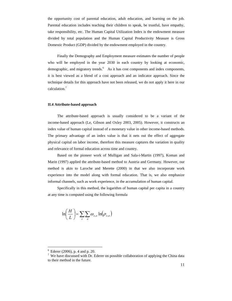
Specifically in this method, the logarithm of human capital per capita in a country

at any time is computed using the following formula

( )∑∑=⎟⎠⎞

⎜⎝⎛

e aaeaeL

H,, lnln ρω

6 Ederer (2006), p. 4 and p. 20. 7 We have discussed with Dr. Ederer on possible collaboration of applying the China data to their method in the future.

12

( )

( )∑∑

∑

∑

=++

++

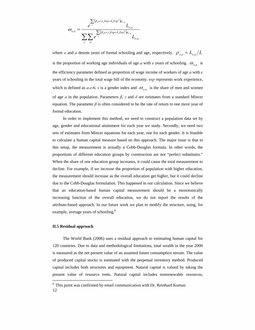
e aae

ExpExpe

ae

ExpExpe

ae

Le

Le

sassss

sassss

,

,,

,2

,2

ϕδγβ

ϕδγβ

ω

where e and a denote years of formal schooling and age, respectively. LL aeae ,, =ρ

is the proportion of working age individuals of age a with e years of schooling. ae,ω is

the efficiency parameter defined as proportion of wage income of workers of age a with e

years of schooling in the total wage bill of the economy. exp represents work experience,

which is defined as a-e-6. s is a gender index and ae,ω is the share of men and women

of age a in the population. Parameters β, γ and δ are estimates from a standard Mincer

equation. The parameter β is often considered to be the rate of return to one more year of

formal education.

In order to implement this method, we need to construct a population data set by

age, gender and educational attainment for each year we study. Secondly, we need two

sets of estimates from Mincer equations for each year, one for each gender. It is feasible

to calculate a human capital measure based on this approach. The major issue is that in

this setup, the measurement is actually a Cobb-Douglas formula. In other words, the

proportions of different education groups by construction are not “perfect substitutes.”

When the share of one education group increases, it could cause the total measurement to

decline. For example, if we increase the proportion of population with higher education,

the measurement should increase as the overall education get higher, but it could decline

due to the Cobb-Douglas formulation. This happened in our calculation. Since we believe

that an education-based human capital measurement should be a monotonically

increasing function of the overall education, we do not report the results of the

attribute-based approach. In our future work we plan to modify the structure, using, for

example, average years of schooling.8

II.5 Residual approach

The World Bank (2006) uses a residual approach to estimating human capital for

120 countries. Due to data and methodological limitations, total wealth in the year 2000

is measured as the net present value of an assumed future consumption stream. The value

of produced capital stocks is estimated with the perpetual inventory method. Produced

capital includes both structures and equipment. Natural capital is valued by taking the

present value of resource rents. Natural capital includes nonrenewable resources, 8 This point was confirmed by email communication with Dr. Reinhard Koman.

13

cropland, pastureland, forested areas, and protected areas. Intangible capital is equal to

total wealth minus produced and natural capital. Intangible capital is an aggregate which

includes human capital, the infrastructure of the country, social capital, and the returns

from net foreign financial assets. Net foreign financial assets are included because debt

interest obligations will affect the level of consumption. Intangible capital represents

greater than 50% of wealth for almost 85% of the countries studied.

Using a net present value approach to estimate total wealth requires assumptions

about the time horizon and the discount rate. The World Bank chooses 25 years as the

time horizon as it roughly corresponds to one generation. It chooses a social discount rate

rather than a private rate as governments would use a social discount rate to allocate

resources across generations. The social discount rate is set at 4%, which is at the upper

range of estimates it reviewed for industrialized countries. The same rate is used for all

countries to facilitate comparisons across countries.

A Cobb-Douglas specification is employed to estimate the marginal returns and

contribution of three types of intangible capital in the model. The model independent

variables include per capita years of schooling of the working population, human capital

abroad, and governance/social capital. Human capital abroad is measured by remittances

by workers outside the country. Governance/social capital is measured with a rule of law

index. Although the marginal return to human capital in the aggregate is the highest of

the three included intangible capital components, the contribution decomposition

demonstrates that the relative contributions can differ significantly across countries

(World Bank, 2006, chapter 7).

III. Data

III.1 Population

In order to implement the various methods used in estimating human capital, we

first and foremost need annual population data by age, sex, and educational attainment.

We construct such data sets according to the following procedure.

First, data sets are available for the years 1982, 1987, 1990, 1995, 2000, and 2005.

They are reported in various issues of Population Census, Population Sampling Survey,

and Population Yearbooks. The data sets also contain disaggregated numbers for urban

and rural populations.

For all other years, we collect population data by age and sex from various issues

of China Population Yearbooks. Then we combine birth rate (China Statistical Yearbook),

mortality rate by age and sex (China Population Yearbook), and enrollment (including

new enrollment and graduation, China Education Statistical Yearbook) at different levels

14

of education to impute population by age, sex and educational attainment for each and

every year. We define the following levels of educational attainment: illiterate (no

schooling), primary school (Grade 1-6), junior middle school (Grade 7-9), senior middle

school (Grade 10-12), and college and above. From 2000 on, additional information

makes it possible to separate the population at the level of college and above into two:

one is college, and the other is university and above.

Specifically, we use the following perpetual inventory formula to deduce

population by age, sex and educational attainment in missing years:

( ) ( ) ( )( ) ( )( ) ( )

, , , 1, , , 1 , , , , ,

, , , , , ,

L y e a s L y e a s y a s IF y e a s

OF y e a s EX y e a s

δ= − ⋅ − +

− +

L(y,e,a,s) is the population in year y at education level e, with age a and sex s. δ(y,a,s) is

the mortality rate in year y, with age a and sex s. IF(y,e,a,s) and OF(y,e,a,s) are inflow

and outflow of this particular group. For example, inflow would include individuals just

achieved this level of education, while outflow would include those who just achieved the

next level of education. EX(y,e,a,s) is a discrepancy term. Moreover,

( ) ( ) ( )seyERSsaeysaeyIF ,,,,,,,, ⋅= λ

( ) ( ) ( )seyERSsaeysaeyOF ,1,,,1,,,, +⋅+= λ

( ) 1,,, =∑a

saeyλ

ERS is the matriculation at education level e, λ is the age distribution at education level e.

In order to obtain accurate estimate for λ, we use both microeconomic data sets (China

Health and Nutrition Survey and China Household Income Project) and macroeconomic

data sets (China Education Statistical Yearbook). Next we discuss several salient features

of China’s population growth, especially the educational attainment by age, sex, and

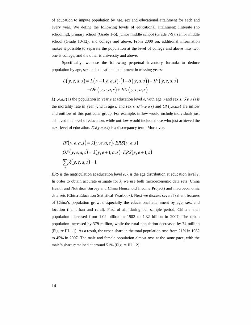
location (i.e. urban and rural). First of all, during our sample period, China’s total

population increased from 1.02 billion in 1982 to 1.32 billion in 2007. The urban

population increased by 379 million, while the rural population decreased by 74 million

(Figure III.1.1). As a result, the urban share in the total population rose from 21% in 1982

to 45% in 2007. The male and female population almost rose at the same pace, with the

male’s share remained at around 51% (Figure III.1.2).

15

Figure III.1.1 Population in China, 1982-2007

0

300

600

900

1200

1500

1982 1984 1986 1988 1990 1992 1994 1996 1998 2000 2002 2004 2006year

mill

ions

total urban rural

Figure III.1.2 Population in China, 1982-2007

0

300

600

900

1200

1500

1982 1984 1986 1988 1990 1992 1994 1996 1998 2000 2002 2004 2006

year

millions

total male female

Figure III.1.3 Population by educational attainment, 1982-2007

0

100

200

300

400

500

1982 1984 1986 1988 1990 1992 1994 1996 1998 2000 2002 2004 2006

year

millio

ns

no schooling primary school junior middle school

senior middle school college and over

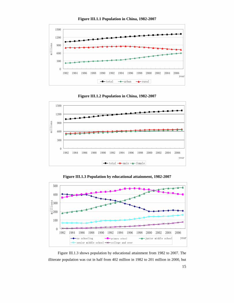
Figure III.1.3 shows population by educational attainment from 1982 to 2007. The

illiterate population was cut in half from 402 million in 1982 to 201 million in 2000, but

16

was relatively stable from 2000 to 2007. The number of primary school graduates

increased from 359 million in 1982 to the peak of 466 million in 1997, then declined

gradually to 399 million in 2007. This decline is expected as more primary school

graduates continue on to higher education level instead of terminating formal education.

This is also evident in the rapid growth of junior middle school graduates.

Junior middle school students registered the largest growth among all education

levels: the number of junior middle school graduates increased from 181 million in 1982

to 471 million in 2007. This might be related to the implementation of 9-Year

Compulsory Schooling since 1994 (9-year schooling amounts to completing junior

middle school). However, the growth slowed after 2001. Senior middle school and

college and over, both started from very low numbers and have grown significantly.

Senior middle school graduates increased from 68 million in 1982 to 166 million in 2007,

while college and above increased from only 6 million in 1982 to 76 million in 2007.

Figure III.1.4 Population of different educational levels by gender, 1982

0

100

200

300

400

500

no schooling primary

school

junior middle

school

senior middle

school

college and

over

millions

male female total

Figure III.1.5 Population of different educational levels by gender, 1988

0

100

200

300

400

500

no schooling primary school junior middleschool

senior middleschool

college and over

mill

ions

male female total

17

Figure III.1.6 Population of different educational levels by gender, 1998

0

100

200

300

400

500

no schooling primary school junior middleschool

senior middleschool

college and over

mill

ions

male female total

Figure III.1.7 Population of different educational levels by gender, 2007

0

100

200

300

400

500

no schooling primary school junior middleschool

senior middleschool

college and over

mill

ions

male female total

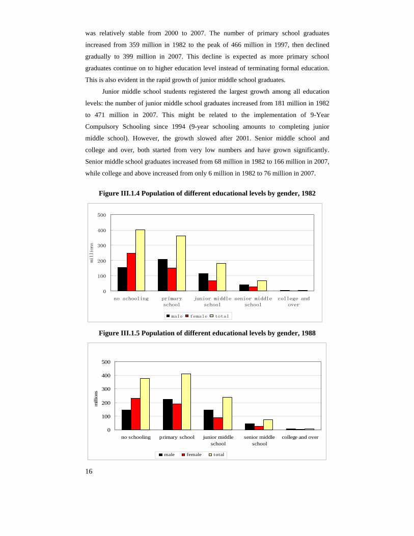
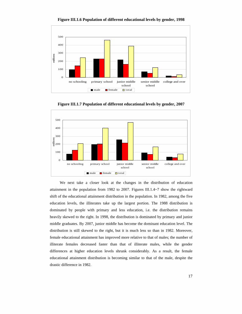
We next take a closer look at the changes in the distribution of education

attainment in the population from 1982 to 2007. Figures III.1.4~7 show the rightward

shift of the educational attainment distribution in the population. In 1982, among the five

education levels, the illiterates take up the largest portion. The 1988 distribution is

dominated by people with primary and less education, i.e. the distribution remains

heavily skewed to the right. In 1998, the distribution is dominated by primary and junior

middle graduates. By 2007, junior middle has become the dominant education level. The

distribution is still skewed to the right, but it is much less so than in 1982. Moreover,

female educational attainment has improved more relative to that of males; the number of

illiterate females decreased faster than that of illiterate males, while the gender

differences at higher education levels shrunk considerably. As a result, the female

educational attainment distribution is becoming similar to that of the male, despite the

drastic difference in 1982.

18

Figure III.1.8 Population of different educational levels by urban and rural, 1982

0

100

200

300

400

500

no schooling primary

school

junior middle

school

senior middle

school

college and

over

millions

urban rural total

Figure III.1.9 Population of different educational levels by urban and rural, 1988

0

100

200

300

400

500

no schooling primary school junior middleschool

senior middleschool

college and over

mill

ions

urban rural total

Figure III.1.10 Population of different educational levels by urban and rural, 1998

0

100

200

300

400

500

no schooling primary school junior middleschool

senior middleschool

college and over

mill

ions

urban rural total

19

Figure III.1.11 Population of different educational levels by urban and rural, 2007

0

100

200

300

400

500

no schooling primary school junior middleschool

senior middleschool

college and over

mill

ions

urban rural total

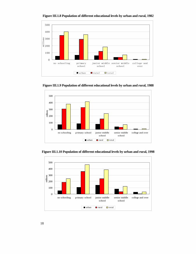
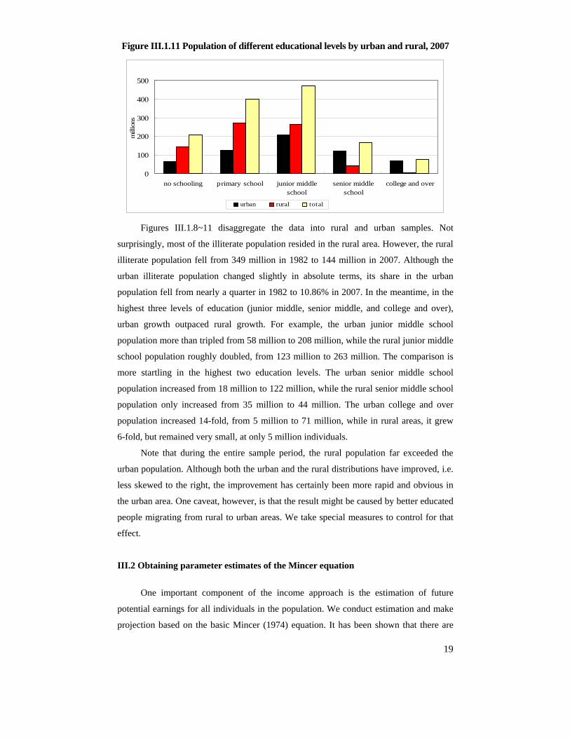
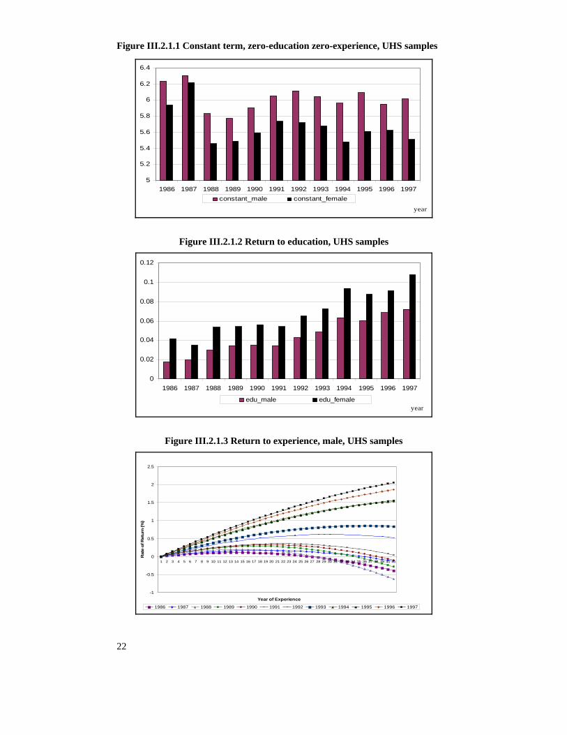
Figures III.1.8~11 disaggregate the data into rural and urban samples. Not

surprisingly, most of the illiterate population resided in the rural area. However, the rural

illiterate population fell from 349 million in 1982 to 144 million in 2007. Although the

urban illiterate population changed slightly in absolute terms, its share in the urban

population fell from nearly a quarter in 1982 to 10.86% in 2007. In the meantime, in the

highest three levels of education (junior middle, senior middle, and college and over),

urban growth outpaced rural growth. For example, the urban junior middle school

population more than tripled from 58 million to 208 million, while the rural junior middle

school population roughly doubled, from 123 million to 263 million. The comparison is

more startling in the highest two education levels. The urban senior middle school

population increased from 18 million to 122 million, while the rural senior middle school

population only increased from 35 million to 44 million. The urban college and over

population increased 14-fold, from 5 million to 71 million, while in rural areas, it grew

6-fold, but remained very small, at only 5 million individuals.

Note that during the entire sample period, the rural population far exceeded the

urban population. Although both the urban and the rural distributions have improved, i.e.

less skewed to the right, the improvement has certainly been more rapid and obvious in

the urban area. One caveat, however, is that the result might be caused by better educated

people migrating from rural to urban areas. We take special measures to control for that

effect.

III.2 Obtaining parameter estimates of the Mincer equation

One important component of the income approach is the estimation of future

potential earnings for all individuals in the population. We conduct estimation and make

projection based on the basic Mincer (1974) equation. It has been shown that there are

20

significant differences in the structure of the earnings equation across gender and

between the rural and urban population. To ensure our income estimates to be as accurate

as possible, we estimate the parameters for the rural and urban population by gender and

year using survey data in selected years and derive their imputed values for missing years

over the period of 1985 to 2020.

We first estimate the basic Mincer equation:

( ) 2ln inc e exp exp uα β γ δ= + ⋅ + ⋅ + ⋅ + （1）

where ln(inc) is the logarithm of earnings, e is years of schooling, exp and exp2 are,

respectively, years of work experience and experience squared, and u is a random error.

The coefficient α is an estimate of the average log earnings of individuals with zero years

of schooling and work experience, β is an estimate of the return to an extra year of

schooling, and γ and δ measure the return to investment in on-the-job training.

Equation (1) has been the workhorse widely adopted in empirical research on

earnings determination. It has been estimated on a large number of data sets for numerous

countries and time periods. Many studies have applied the model to Chinese data and

found evidence consistent with the human capital theory. Notable studies include, among

others, Liu (1998), Maurer-Fazio (1999), Li (2003), Fleisher and Wang (2004), Yang

(2005), and Zhang et al. (2005). Following the convention of a large body of empirical

literature, we estimate equation (1) by ordinary least squares.9

The data used for estimating the parameters of the earnings equation come from

two well-known household surveys in China. The first is the annual Urban Household

Survey (UHS) conducted by the National Statistical Bureau of China over the period of

1986-1997. We use this data set to estimate the parameters of equation (1) for each

gender of the urban population by year, and then extract fitted estimates by applying

linear or exponential time trends. We use the fitted time trends to generate the imputed

parameters of the earnings equation for the urban population for the period 1985 through

2020.

The second data set we use is the China Health and Nutrition Survey (CHNS) for

the years of 1989, 1991, 1993, 1997, and 2000. This survey covers both the urban and

rural population. We use CHNS to obtain earnings-equation parameter estimates by year

for each gender and separately for the rural and urban population. We calculate the

urban-to-rural ratio for each of these parameters. We then use the ratio to fit a time trend

model (i.e. interpolate and extrapolate), which is used to generate fitted values of the 9 Griliches (1977) finds that accounting for the endogeneity of schooling and ability bias does not alter the estimates of earnings equation. Ashenfelter and Krueger (1994) also conclude that omitted ability variables do not cause an upward bias in the estimated parameters of equation (1).

21

urban-to-rural ratio over the period 1985 to 2020. We use the fitted ratios along with the

imputed parameters for the urban population to derive the imputed parameters for the

rural population over the period 1985 to 2020.

III.2.1 Imputing the earnings equation parameters for the urban population

The UHS is a representative sample of the urban population. The sample size

varies from year to year, ranging from a low of 4,934 respondents in 1986 to a high of

31,266 respondents in 1992. Individual earnings are annual wage incomes, which include

basic wage, bonus, subsidies and other work-related incomes. Years of schooling are

calculated using the information on the level of schooling completed: primary school

equals 6 years of schooling, junior middle school 9 years, senior middle school 12 years,

professional school 11 years, community college 15 years, and college and above 16

years. Assuming schooling begins at age 6, we approximate work experience by age

minus years of schooling minus 6. As the minimum legal working age is 16 and the

retirement ages are 60 and 55 for males and females respectively, we restrict our sample

to include individuals who are currently employed and are between 16 and 60 years of

age for male workers and between 16 and 55 for female workers. Self-employed and

temporary job holders are excluded, so are those who failed to report wage income or

educational attainment.

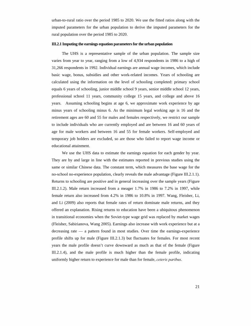
We use the UHS data to estimate the earnings equation for each gender by year.

They are by and large in line with the estimates reported in previous studies using the

same or similar Chinese data. The constant term, which measures the base wage for the

no-school no-experience population, clearly reveals the male advantage (Figure III.2.1.1).

Returns to schooling are positive and in general increasing over the sample years (Figure

III.2.1.2). Male return increased from a meager 1.7% in 1986 to 7.2% in 1997, while

female return also increased from 4.2% in 1986 to 10.8% in 1997. Wang, Fleisher, Li,

and Li (2009) also reports that female rates of return dominate male returns, and they

offered an explanation. Rising returns to education have been a ubiquitous phenomenon

in transitional economies when the Soviet-type wage grid was replaced by market wages

(Fleisher, Sabirianova, Wang 2005). Earnings also increase with work experience but at a

decreasing rate — a pattern found in most studies. Over time the earnings-experience

profile shifts up for male (Figure III.2.1.3) but fluctuates for females. For most recent

years the male profile doesn’t curve downward as much as that of the female (Figure

III.2.1.4), and the male profile is much higher than the female profile, indicating

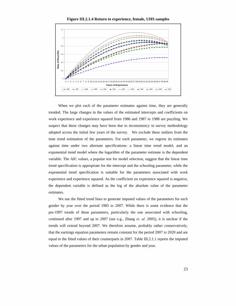
uniformly higher return to experience for male than for female, ceteris paribus.

22

Figure III.2.1.1 Constant term, zero-education zero-experience, UHS samples

5

5.2

5.4

5.6

5.8

6

6.2

6.4

1986 1987 1988 1989 1990 1991 1992 1993 1994 1995 1996 1997

year

constant_male constant_female

Figure III.2.1.2 Return to education, UHS samples

0

0.02

0.04

0.06

0.08

0.1

0.12

1986 1987 1988 1989 1990 1991 1992 1993 1994 1995 1996 1997

yearedu_male edu_female

Figure III.2.1.3 Return to experience, male, UHS samples

-1

-0.5

0

0.5

1

1.5

2

2.5

1 2 3 4 5 6 7 8 9 10 11 12 13 14 15 16 17 18 19 20 21 22 23 24 25 26 27 28 29 30 31 32 33 34 35 36 37 38 39 40 41

Year of Experience

Rat

e of

Ret

urn

(%)

1986 1987 1988 1989 1990 1991 1992 1993 1994 1995 1996 1997

23

Figure III.2.1.4 Return to experience, female, UHS samples

0

0.2

0.4

0.6

0.8

1

1.2

0 1 2 3 4 5 6 7 8 9 10 11 12 13 14 15 16 17 18 19 20 21 22 23 24 25 26 27 28 29 30 31 32 33 34 35 36 37 38 39 40

Years of Experience

Rat

e of

Reu

rn(%

)

1986 1987 1988 1989 1990 1991 1992 1993 1994 1995 1996 1997

When we plot each of the parameter estimates against time, they are generally

trended. The large changes in the values of the estimated intercepts and coefficients on

work experience and experience squared from 1986 and 1987 to 1988 are puzzling. We

suspect that these changes may have been due to inconsistency in survey methodology

adopted across the initial few years of the survey. We exclude these outliers from the

time trend estimation of the parameters. For each parameter, we regress its estimates

against time under two alternate specifications: a linear time trend model, and an

exponential trend model where the logarithm of the parameter estimate is the dependent

variable. The AIC values, a popular test for model selection, suggest that the linear time

trend specification is appropriate for the intercept and the schooling parameter, while the

exponential trend specification is suitable for the parameters associated with work

experience and experience squared. As the coefficient on experience squared is negative,

the dependent variable is defined as the log of the absolute value of the parameter

estimates.

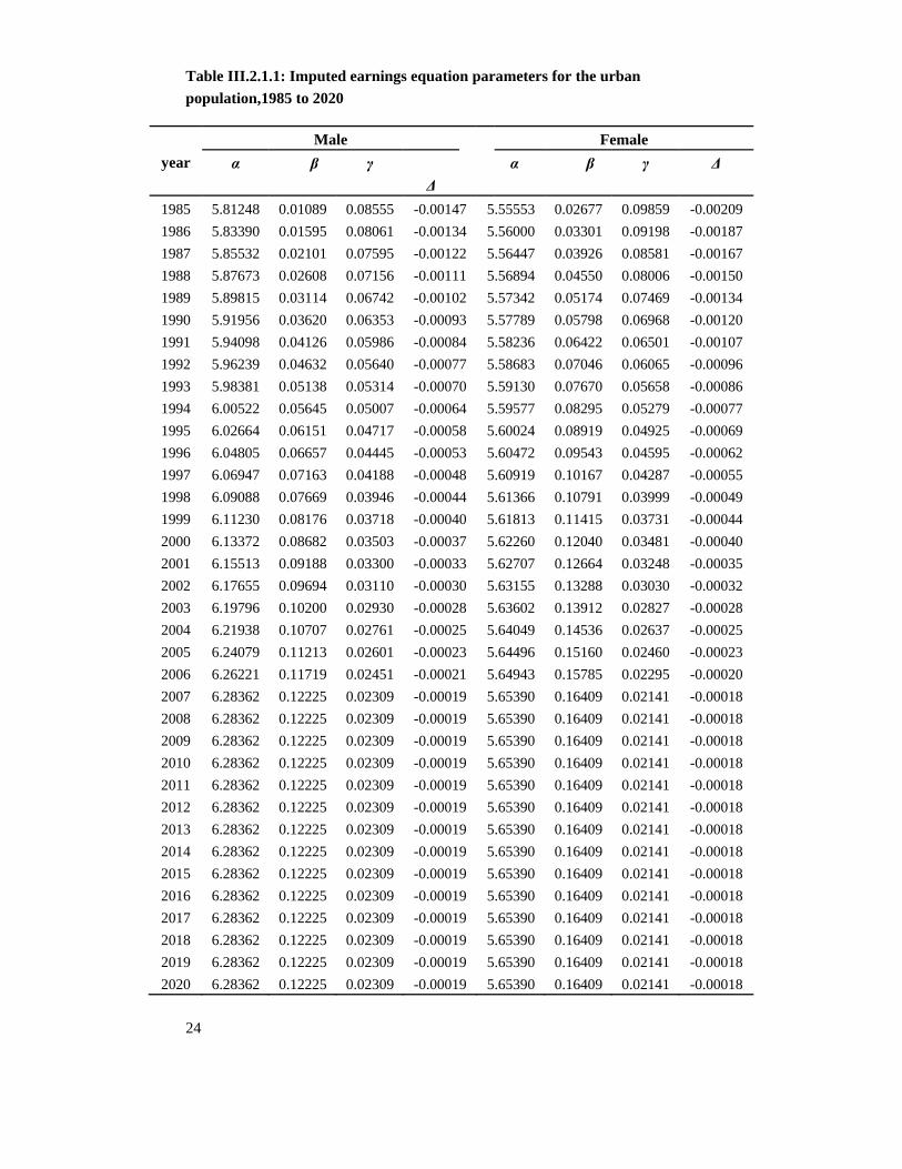
We use the fitted trend lines to generate imputed values of the parameters for each

gender by year over the period 1985 to 2007. While there is some evidence that the

pre-1997 trends of these parameters, particularly the one associated with schooling,

continued after 1997 and up to 2007 (see e.g., Zhang et. al. 2005), it is unclear if the

trends will extend beyond 2007. We therefore assume, probably rather conservatively,

that the earnings equation parameters remain constant for the period 2007 to 2020 and are

equal to the fitted values of their counterparts in 2007. Table III.2.1.1 reports the imputed

values of the parameters for the urban population by gender and year.

24

Table III.2.1.1: Imputed earnings equation parameters for the urban population,1985 to 2020

year Male Female

α β γ Δ

α β γ Δ

1985 5.81248 0.01089 0.08555 -0.00147 5.55553 0.02677 0.09859 -0.00209 1986 5.83390 0.01595 0.08061 -0.00134 5.56000 0.03301 0.09198 -0.00187 1987 5.85532 0.02101 0.07595 -0.00122 5.56447 0.03926 0.08581 -0.00167 1988 5.87673 0.02608 0.07156 -0.00111 5.56894 0.04550 0.08006 -0.00150 1989 5.89815 0.03114 0.06742 -0.00102 5.57342 0.05174 0.07469 -0.00134 1990 5.91956 0.03620 0.06353 -0.00093 5.57789 0.05798 0.06968 -0.00120 1991 5.94098 0.04126 0.05986 -0.00084 5.58236 0.06422 0.06501 -0.00107 1992 5.96239 0.04632 0.05640 -0.00077 5.58683 0.07046 0.06065 -0.00096 1993 5.98381 0.05138 0.05314 -0.00070 5.59130 0.07670 0.05658 -0.00086 1994 6.00522 0.05645 0.05007 -0.00064 5.59577 0.08295 0.05279 -0.00077 1995 6.02664 0.06151 0.04717 -0.00058 5.60024 0.08919 0.04925 -0.00069 1996 6.04805 0.06657 0.04445 -0.00053 5.60472 0.09543 0.04595 -0.00062 1997 6.06947 0.07163 0.04188 -0.00048 5.60919 0.10167 0.04287 -0.00055 1998 6.09088 0.07669 0.03946 -0.00044 5.61366 0.10791 0.03999 -0.00049 1999 6.11230 0.08176 0.03718 -0.00040 5.61813 0.11415 0.03731 -0.00044 2000 6.13372 0.08682 0.03503 -0.00037 5.62260 0.12040 0.03481 -0.00040 2001 6.15513 0.09188 0.03300 -0.00033 5.62707 0.12664 0.03248 -0.00035 2002 6.17655 0.09694 0.03110 -0.00030 5.63155 0.13288 0.03030 -0.00032 2003 6.19796 0.10200 0.02930 -0.00028 5.63602 0.13912 0.02827 -0.00028 2004 6.21938 0.10707 0.02761 -0.00025 5.64049 0.14536 0.02637 -0.00025 2005 6.24079 0.11213 0.02601 -0.00023 5.64496 0.15160 0.02460 -0.00023 2006 6.26221 0.11719 0.02451 -0.00021 5.64943 0.15785 0.02295 -0.00020 2007 6.28362 0.12225 0.02309 -0.00019 5.65390 0.16409 0.02141 -0.00018 2008 6.28362 0.12225 0.02309 -0.00019 5.65390 0.16409 0.02141 -0.00018 2009 6.28362 0.12225 0.02309 -0.00019 5.65390 0.16409 0.02141 -0.00018 2010 6.28362 0.12225 0.02309 -0.00019 5.65390 0.16409 0.02141 -0.00018 2011 6.28362 0.12225 0.02309 -0.00019 5.65390 0.16409 0.02141 -0.00018 2012 6.28362 0.12225 0.02309 -0.00019 5.65390 0.16409 0.02141 -0.00018 2013 6.28362 0.12225 0.02309 -0.00019 5.65390 0.16409 0.02141 -0.00018 2014 6.28362 0.12225 0.02309 -0.00019 5.65390 0.16409 0.02141 -0.00018 2015 6.28362 0.12225 0.02309 -0.00019 5.65390 0.16409 0.02141 -0.00018 2016 6.28362 0.12225 0.02309 -0.00019 5.65390 0.16409 0.02141 -0.00018 2017 6.28362 0.12225 0.02309 -0.00019 5.65390 0.16409 0.02141 -0.00018 2018 6.28362 0.12225 0.02309 -0.00019 5.65390 0.16409 0.02141 -0.00018 2019 6.28362 0.12225 0.02309 -0.00019 5.65390 0.16409 0.02141 -0.00018 2020 6.28362 0.12225 0.02309 -0.00019 5.65390 0.16409 0.02141 -0.00018

25

III.2.2 Imputing the earnings equation parameters for the rural population

The CHNS is an ongoing international collaborative project between the Carolina

Population Center at the University of North Carolina at Chapel Hill and the National

Institute of Nutrition and Food Safety at the Chinese Center for Disease Control and

Prevention and was designed for evaluating the impact of social and economic

transformation of the Chinese society on socioeconomic, demographic, and health

behaviors of the urban and rural population. The survey also contains information on

income, age and educational attainment, which we use to estimate the earnings equation

by year for each gender and separately for the urban and rural population. For the urban

sample, earnings contain wage income and subsidies from work.

The rural sample contains only household income, which includes family

members’ incomes from the collective or household productions or both in five distinct

activities: gardening, farming, raising livestock, fishing, and small handicraft and family

businesses. We allocate household income to each individual member according to his or

her working hours as a share of the household’s total. Years of schooling are calculated

based on the reported grade or years completed (depending on the sample year). Work

experience is approximated by age minus years of schooling minus 6. We restrict our

sample to males between 16 and 60 years of age and females between 16 and 55 who

reported information on education and income.

We use the CHNS data to estimate equation (1) by gender and separately for the

rural and urban samples for each of the sample year (i.e., 1989, 1991, 1993, 1997, and

2000). The parameter estimates are then used to calculate the urban-to-rural ratio for each

parameter by gender. We use the ratios to fit an exponential trend model, which is used to

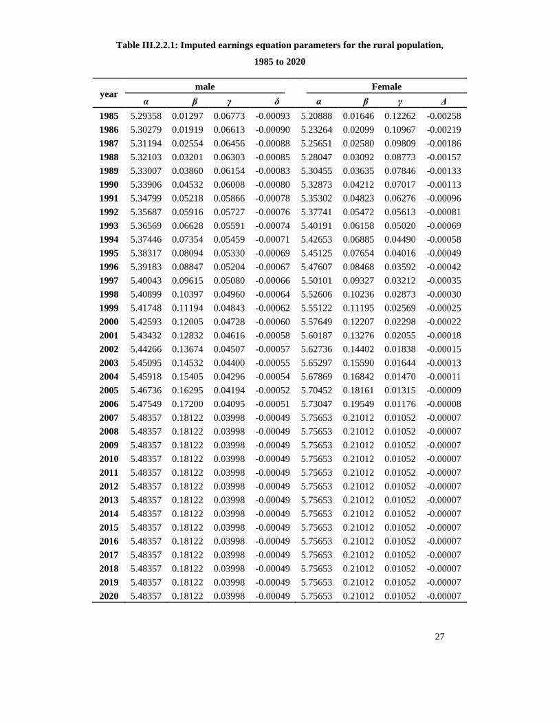
generate the fitted ratios for the period 1985 to 2007. We assume that the ratios remain

constant for the period 2007 to 2020 and are equal to the fitted values of their

counterparts in 1997. The fitted urban-to-rural ratios by themselves provide interesting

insights. For example, in 1985, the urban no-schooling no-experience male cohort was on

average paid 9.8% more than its rural counterpart, and by 2007 this gap has increased to

14.6%. In the meantime, the urban no-schooling no-experience female cohort was on

average paid 6.7% more than its rural counterpart, and by 2007 the rural cohort was paid

1.8% more than the urban cohort. Return to education is always higher for rural male than

for urban male. In 1985, the rate of return was 16% higher for rural male, and by 2007 it

was 33% higher. For female, however, it is a different story. Return to education for

urban female was 63% higher than rural female, but by 2007 the return to urban female

was 22% less than rural female. The relation between urban and rural return to experience

has also changed. All of these are not central to our current project, but nevertheless

deserves attention in future research.

26

We use these ratios along with the imputed parameters for the urban population in

Table III.2.1.1 to impute parameters for the rural population which are presented in Table

III.2.2.1.

27

Table III.2.2.1: Imputed earnings equation parameters for the rural population,

1985 to 2020

year male Female

α β γ δ α β γ Δ 1985 5.29358 0.01297 0.06773 -0.00093 5.20888 0.01646 0.12262 -0.00258 1986 5.30279 0.01919 0.06613 -0.00090 5.23264 0.02099 0.10967 -0.00219 1987 5.31194 0.02554 0.06456 -0.00088 5.25651 0.02580 0.09809 -0.00186 1988 5.32103 0.03201 0.06303 -0.00085 5.28047 0.03092 0.08773 -0.00157 1989 5.33007 0.03860 0.06154 -0.00083 5.30455 0.03635 0.07846 -0.00133 1990 5.33906 0.04532 0.06008 -0.00080 5.32873 0.04212 0.07017 -0.00113 1991 5.34799 0.05218 0.05866 -0.00078 5.35302 0.04823 0.06276 -0.00096 1992 5.35687 0.05916 0.05727 -0.00076 5.37741 0.05472 0.05613 -0.00081 1993 5.36569 0.06628 0.05591 -0.00074 5.40191 0.06158 0.05020 -0.00069 1994 5.37446 0.07354 0.05459 -0.00071 5.42653 0.06885 0.04490 -0.00058 1995 5.38317 0.08094 0.05330 -0.00069 5.45125 0.07654 0.04016 -0.00049 1996 5.39183 0.08847 0.05204 -0.00067 5.47607 0.08468 0.03592 -0.00042 1997 5.40043 0.09615 0.05080 -0.00066 5.50101 0.09327 0.03212 -0.00035 1998 5.40899 0.10397 0.04960 -0.00064 5.52606 0.10236 0.02873 -0.00030 1999 5.41748 0.11194 0.04843 -0.00062 5.55122 0.11195 0.02569 -0.00025 2000 5.42593 0.12005 0.04728 -0.00060 5.57649 0.12207 0.02298 -0.00022 2001 5.43432 0.12832 0.04616 -0.00058 5.60187 0.13276 0.02055 -0.00018 2002 5.44266 0.13674 0.04507 -0.00057 5.62736 0.14402 0.01838 -0.00015 2003 5.45095 0.14532 0.04400 -0.00055 5.65297 0.15590 0.01644 -0.00013 2004 5.45918 0.15405 0.04296 -0.00054 5.67869 0.16842 0.01470 -0.00011 2005 5.46736 0.16295 0.04194 -0.00052 5.70452 0.18161 0.01315 -0.00009 2006 5.47549 0.17200 0.04095 -0.00051 5.73047 0.19549 0.01176 -0.00008 2007 5.48357 0.18122 0.03998 -0.00049 5.75653 0.21012 0.01052 -0.00007 2008 5.48357 0.18122 0.03998 -0.00049 5.75653 0.21012 0.01052 -0.00007 2009 5.48357 0.18122 0.03998 -0.00049 5.75653 0.21012 0.01052 -0.00007 2010 5.48357 0.18122 0.03998 -0.00049 5.75653 0.21012 0.01052 -0.00007 2011 5.48357 0.18122 0.03998 -0.00049 5.75653 0.21012 0.01052 -0.00007 2012 5.48357 0.18122 0.03998 -0.00049 5.75653 0.21012 0.01052 -0.00007 2013 5.48357 0.18122 0.03998 -0.00049 5.75653 0.21012 0.01052 -0.00007 2014 5.48357 0.18122 0.03998 -0.00049 5.75653 0.21012 0.01052 -0.00007 2015 5.48357 0.18122 0.03998 -0.00049 5.75653 0.21012 0.01052 -0.00007 2016 5.48357 0.18122 0.03998 -0.00049 5.75653 0.21012 0.01052 -0.00007 2017 5.48357 0.18122 0.03998 -0.00049 5.75653 0.21012 0.01052 -0.00007 2018 5.48357 0.18122 0.03998 -0.00049 5.75653 0.21012 0.01052 -0.00007 2019 5.48357 0.18122 0.03998 -0.00049 5.75653 0.21012 0.01052 -0.00007 2020 5.48357 0.18122 0.03998 -0.00049 5.75653 0.21012 0.01052 -0.00007

28

III.3 Growth rates of real income and the discount rate

To measure lifetime earnings for all individuals in the population, we need to

project incomes for future years, discount these incomes back to the present, and weight

income for each individual by the age- and gender-specific probability of survival. We

use the imputed earnings equation parameters to estimate earnings for all individuals in a

given year, and then derive earnings for future years until retirement assuming real

earnings grow at a constant rate.10 The main task of this section is to estimate the

expected growth rate of real income and select an appropriate discount rate. Since the real

income grew at fairly different rates in the past for the urban and rural population, we

estimate them separately.

III.3.1 Growth rates of real income

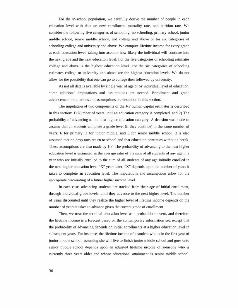
Assuming that the technology is labor-augmenting, we specify the aggregate

production function as:

( )a bY AL K=

where Y is output, A denotes a technology factor, L denotes labor input, and K physical

capital input. The average product of labor or labor productivity is proportional to the

marginal product of labor.11 Because the marginal product of labor equals the real wage

when the labor market is in equilibrium, labor productivity and the real wage are

expected to grow at the same rate. Therefore, the growth rate of real output per employed

worker can serve as a reasonable estimate for the growth rate of the real wage.

National Statistical Bureau of China publishes nominal GDP and real GDP index

(in 1978 prices) by sector (primary industry, secondary industry, and tertiary industry).

We derive real GDP as the product of nominal GDP in the base year and real GDP index.

The labor productivity in the rural sector is defined as real GDP of the primary industry

divided by the number of persons employed in the primary industry. The labor

productivity in the urban sector is the ratio of real GDP of the secondary and tertiary

industries to the number of persons employed in these industries.

10 Mincer equation parameter estimates are used to calculate the cohort-wise labor income for a given year, it is not used to project future income. 11 The marginal product of labor is given by βQ/L, where Q/L is the average product of labor.

29

In the past 30 years labor productivity grew on average 4.11% and 6% per annum

in the rural and urban sectors, respectively. We assume labor productivities (and hence

the real income) continue to grow annually at these average rates.12

III.3.2 The discount rate

The discount rate that is used to value future incomes in present terms should

reflect the rate of return one expects from investments over a long time horizon. In this

regard, the interest rate paid on government bonds is a good proxy. We choose a discount

rate of 3.14%, which is the average interest rate on the 10-year government bonds issued

to individual investors over the period 1996 to 2007, net of the average rate of inflation

over the same period. It should be noted that our discount rate is lower than the discount

rates used in the Jorgenson and Fraumeni studies cited in this report.

III.4 Additional data imputations and assumptions for the Jorgenson- Fraumeni

estimates

Besides annual population data by age, sex, and educational attainment, the

Jorgenson-Fraumeni method requires additional information on the lifetime income,

enrollment rate, growth rate of real wage, and discount rate. We briefly discuss how we

construct these supplemental data sets in this section. Some parameters have to be set at

values appropriate for China.

Following Jorgenson and Fraumeni, an individual may assume one of the following

six statuses at any time: no school or work (age 0-5), school only (age 6-16), work and

school (age 16 to age), work only (age to retirement), and retirement (age 60+ for male

and 55+ for female). Each status implies a different pattern of age-income profile,

therefore the method of computing lifetime income shall be different.

We first estimate a standard Mincer equation (i.e. with a regression of annual

income on schooling years, work experience, and work experience squared) with

microeconomic data sets (China Household Income Project, China Health and Nutrition

Survey, and Urban Household Survey). We use annual employment rates by age, sex, and

educational attainment (from China Population Statistical Yearbook and China

Population Census) to convert annual income into annual market income. Then the

lifetime income for each age/sex/education category can be calculated using the

methodology described in the earlier section.

12 One obvious concern is how fast these rates will converge to the long-run steady-state rates, and what are the long-run steady-state rates. Our future research will address these issues.

30

For the in-school population, we carefully derive the number of people in each

education level with data on new enrollment, mortality rate, and attrition rate. We

consider the following five categories of schooling: no schooling, primary school, junior

middle school, senior middle school, and college and above or for six categories of

schooling college and university and above. We compute lifetime income for every grade

at each education level, taking into account how likely the individual will continue into

the next grade and the next education level. For the five categories of schooling estimates

college and above is the highest education level. For the six categories of schooling

estimates college or university and above are the highest education levels. We do not

allow for the possibility that one can go to college then followed by university.

As not all data is available by single year of age or by individual level of education,

some additional imputations and assumptions are needed. Enrollment and grade

advancement imputations and assumptions are described in this section.

The imputation of two components of the J-F human capital estimates is described

in this section: 1) Number of years until an education category is completed, and 2) The

probability of advancing to the next higher education category. A decision was made to

assume that all students complete a grade level (if they continue) in the same number of

years: 6 for primary, 3 for junior middle, and 3 for senior middle school. It is also

assumed that no drop-outs return to school and that education continues without a break.

These assumptions are also made by J-F. The probability of advancing to the next higher

education level is estimated as the average ratio of the sum of all students of any age in a

year who are initially enrolled to the sum of all students of any age initially enrolled in

the next higher education level “X” years later. “X” depends upon the number of years it

takes to complete an education level. The imputations and assumptions allow for the

appropriate discounting of a future higher income level.

In each case, advancing students are tracked from their age of initial enrollment,

through individual grade levels, until they advance to the next higher level. The number

of years discounted until they realize the higher level of lifetime income depends on the

number of years it takes to advance given the current grade of enrollment.

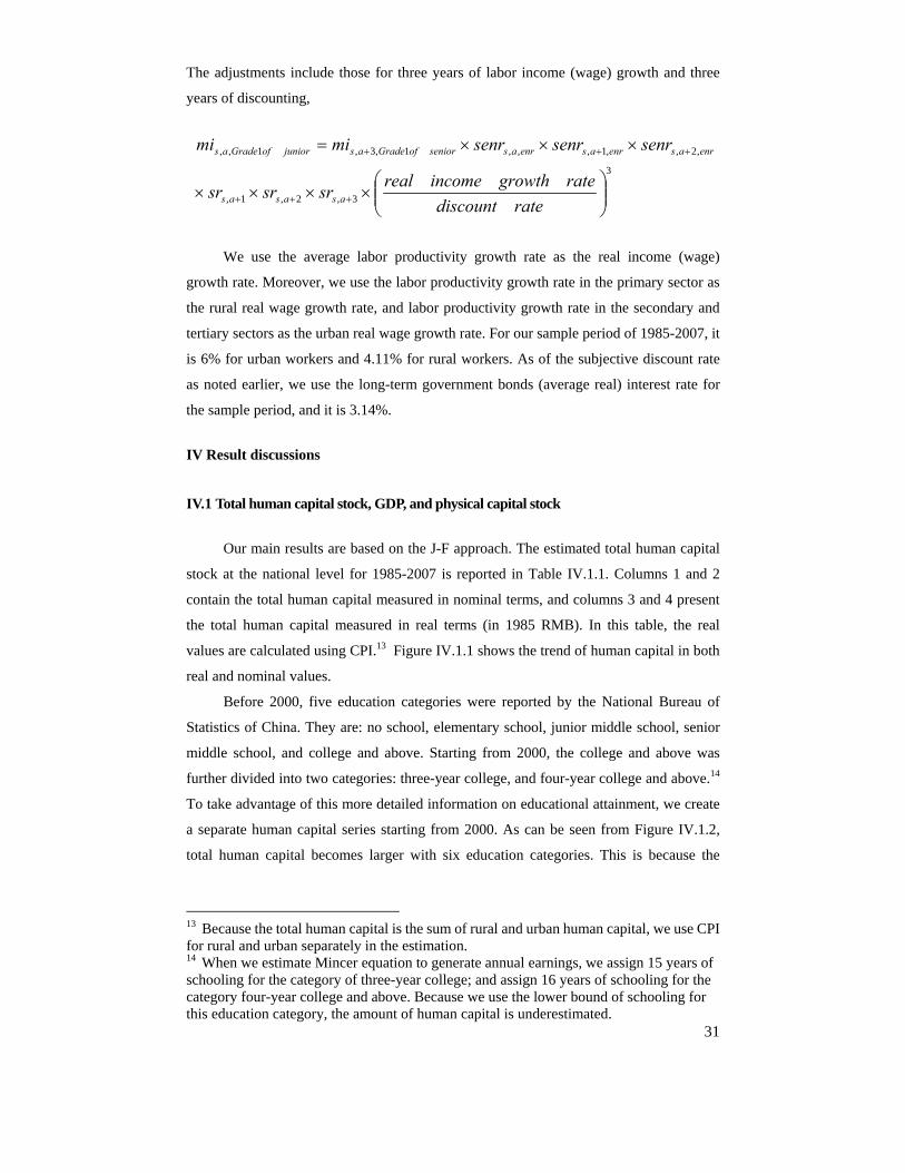
Then, we treat the terminal education level as a probabilistic event, and therefore

the lifetime income is a forecast based on the contemporary information set, except that

the probability of advancing depends on initial enrollments at a higher education level in

subsequent years. For instance, the lifetime income of a student who is in the first year of

junior middle school, assuming she will live to finish junior middle school and goes onto

senior middle school depends upon an adjusted lifetime income of someone who is

currently three years older and whose educational attainment is senior middle school.

31

The adjustments include those for three years of labor income (wage) growth and three

years of discounting,

3

3,2,1,

,2,,1,,,1,3,1,,

⎟⎟⎠

⎞⎜⎜⎝

⎛××××

×××=

+++

+++

ratediscountrategrowthincomerealsrsrsr

senrsenrsenrmimi

asasas

enrasenrasenrasseniorofGradeasjuniorofGradeas

We use the average labor productivity growth rate as the real income (wage)

growth rate. Moreover, we use the labor productivity growth rate in the primary sector as

the rural real wage growth rate, and labor productivity growth rate in the secondary and

tertiary sectors as the urban real wage growth rate. For our sample period of 1985-2007, it

is 6% for urban workers and 4.11% for rural workers. As of the subjective discount rate

as noted earlier, we use the long-term government bonds (average real) interest rate for

the sample period, and it is 3.14%.

IV Result discussions

IV.1 Total human capital stock, GDP, and physical capital stock

Our main results are based on the J-F approach. The estimated total human capital

stock at the national level for 1985-2007 is reported in Table IV.1.1. Columns 1 and 2

contain the total human capital measured in nominal terms, and columns 3 and 4 present

the total human capital measured in real terms (in 1985 RMB). In this table, the real

values are calculated using CPI.13 Figure IV.1.1 shows the trend of human capital in both

real and nominal values.

Before 2000, five education categories were reported by the National Bureau of

Statistics of China. They are: no school, elementary school, junior middle school, senior

middle school, and college and above. Starting from 2000, the college and above was

further divided into two categories: three-year college, and four-year college and above.14

To take advantage of this more detailed information on educational attainment, we create

a separate human capital series starting from 2000. As can be seen from Figure IV.1.2,

total human capital becomes larger with six education categories. This is because the

13 Because the total human capital is the sum of rural and urban human capital, we use CPI for rural and urban separately in the estimation. 14 When we estimate Mincer equation to generate annual earnings, we assign 15 years of schooling for the category of three-year college; and assign 16 years of schooling for the category four-year college and above. Because we use the lower bound of schooling for this education category, the amount of human capital is underestimated.

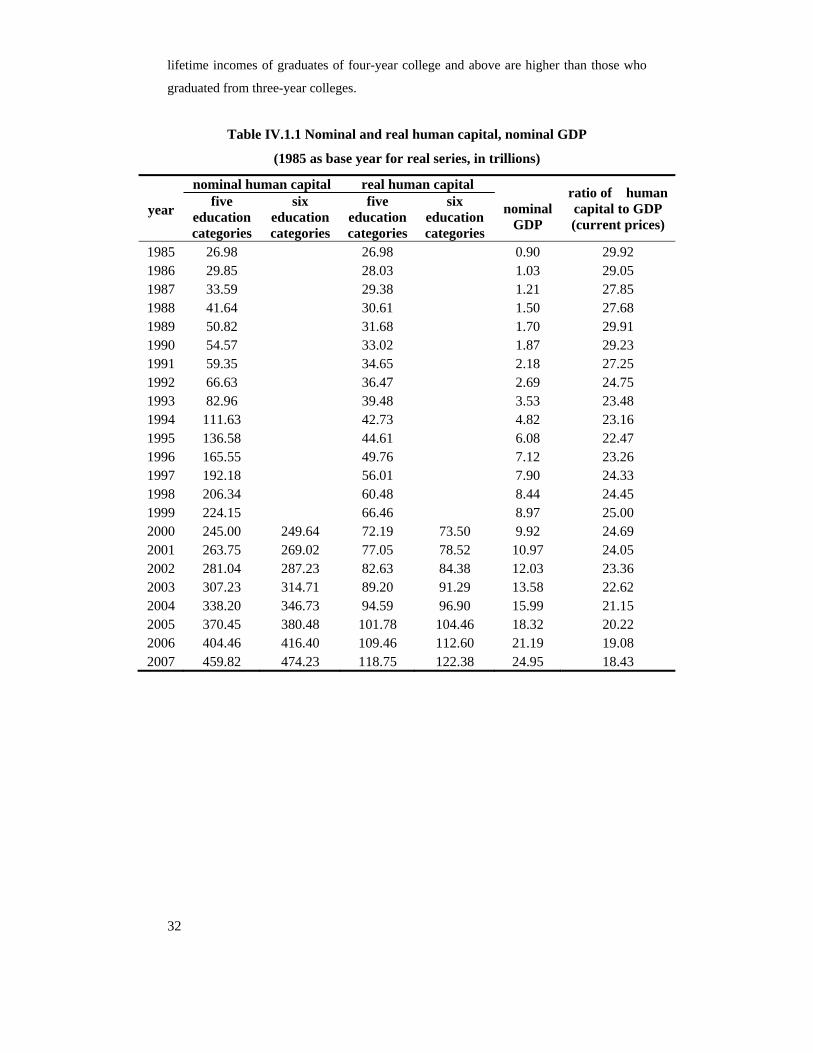
32

lifetime incomes of graduates of four-year college and above are higher than those who

graduated from three-year colleges.

Table IV.1.1 Nominal and real human capital, nominal GDP

(1985 as base year for real series, in trillions)

year

nominal human capital real human capital nominal

GDP

ratio of human capital to GDP (current prices)

five education categories

six education categories

five education categories

six education categories

1985 26.98 26.98 0.90 29.92 1986 29.85 28.03 1.03 29.05 1987 33.59 29.38 1.21 27.85 1988 41.64 30.61 1.50 27.68 1989 50.82 31.68 1.70 29.91 1990 54.57 33.02 1.87 29.23 1991 59.35 34.65 2.18 27.25 1992 66.63 36.47 2.69 24.75 1993 82.96 39.48 3.53 23.48 1994 111.63 42.73 4.82 23.16 1995 136.58 44.61 6.08 22.47 1996 165.55 49.76 7.12 23.26 1997 192.18 56.01 7.90 24.33 1998 206.34 60.48 8.44 24.45 1999 224.15 66.46 8.97 25.00 2000 245.00 249.64 72.19 73.50 9.92 24.69 2001 263.75 269.02 77.05 78.52 10.97 24.05 2002 281.04 287.23 82.63 84.38 12.03 23.36 2003 307.23 314.71 89.20 91.29 13.58 22.62 2004 338.20 346.73 94.59 96.90 15.99 21.15 2005 370.45 380.48 101.78 104.46 18.32 20.22 2006 404.46 416.40 109.46 112.60 21.19 19.08 2007 459.82 474.23 118.75 122.38 24.95 18.43

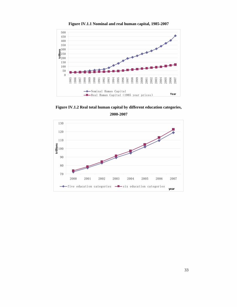
33

Figure IV.1.1 Nominal and real human capital, 1985-2007

0

50

100

150

200

250

300

350

400

450

500

1985

1986

1987

1988

1989

1990

1991

1992

1993

1994

1995

1996

1997

1998

1999

2000

2001

2002

2003

2004

2005

2006

2007

Year

trillions

Nominal Human CapitalReal Human Capital（1985 year prices）

Figure IV.1.2 Real total human capital by different education categories,

2000-2007

70

80

90

100

110

120

130

2000 2001 2002 2003 2004 2005 2006 2007

year

trillions

five education categories six education categories

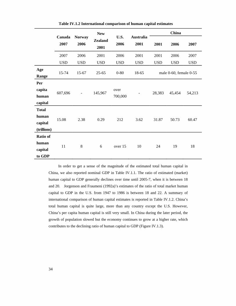
34

Table IV.1.2 International comparison of human capital estimates

Canada

2007

Norway

2006

New

Zealand

2001

U.S.

2006

Australia

2001

China

2001 2006 2007

2007

USD

2006

USD

2001

USD

2006

USD

2001

USD

2001

USD

2006

USD

2007

USD

Age Range

15-74 15-67 25-65 0-80 18-65 male 0-60, female 0-55

Per capita human capital

607,696 - 145,967 over 700,000

- 28,383 45,454 54,213

Total human capital (trillions)

15.08 2.38 0.29 212 3.62 31.87 50.73 60.47

Ratio of human capital to GDP

11 8 6 over 15 10 24 19 18

In order to get a sense of the magnitude of the estimated total human capital in

China, we also reported nominal GDP in Table IV.1.1. The ratio of estimated (market)

human capital to GDP generally declines over time until 2005-7, when it is between 18

and 20. Jorgenson and Fraumeni (1992a)’s estimates of the ratio of total market human

capital to GDP in the U.S. from 1947 to 1986 is between 18 and 22. A summary of

international comparison of human capital estimates is reported in Table IV.1.2. China’s

total human capital is quite large, more than any country except the U.S. However,

China’s per capita human capital is still very small. In China during the later period, the

growth of population slowed but the economy continues to grow at a higher rate, which

contributes to the declining ratio of human capital to GDP (Figure IV.1.3).

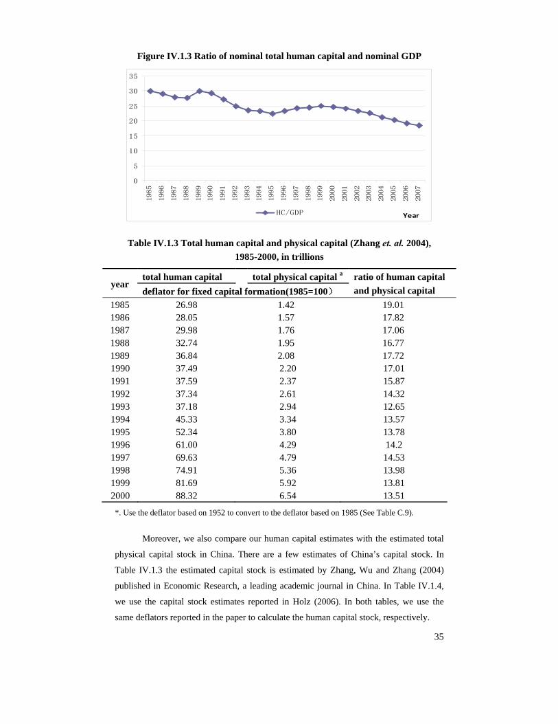
35

Figure IV.1.3 Ratio of nominal total human capital and nominal GDP

0

5

10

15

20

25

30

35

1985

1986

1987

1988

1989

1990

1991

1992

1993

1994

1995

1996

1997

1998

1999

2000

2001

2002

2003

2004

2005

2006

2007

YearHC/GDP

Table IV.1.3 Total human capital and physical capital (Zhang et. al. 2004), 1985-2000, in trillions

year total human capital total physical capital a ratio of human capital

and physical capital deflator for fixed capital formation(1985=100） 1985 26.98 1.42 19.01 1986 28.05 1.57 17.82 1987 29.98 1.76 17.06 1988 32.74 1.95 16.77 1989 36.84 2.08 17.72 1990 37.49 2.20 17.01 1991 37.59 2.37 15.87 1992 37.34 2.61 14.32 1993 37.18 2.94 12.65 1994 45.33 3.34 13.57 1995 52.34 3.80 13.78 1996 61.00 4.29 14.2 1997 69.63 4.79 14.53 1998 74.91 5.36 13.98 1999 81.69 5.92 13.81 2000 88.32 6.54 13.51

*. Use the deflator based on 1952 to convert to the deflator based on 1985 (See Table C.9).

Moreover, we also compare our human capital estimates with the estimated total

physical capital stock in China. There are a few estimates of China’s capital stock. In

Table IV.1.3 the estimated capital stock is estimated by Zhang, Wu and Zhang (2004)

published in Economic Research, a leading academic journal in China. In Table IV.1.4,

we use the capital stock estimates reported in Holz (2006). In both tables, we use the

same deflators reported in the paper to calculate the human capital stock, respectively.

36

As can be seen in Figure IV.1.4 and Figure IV.1.5, in both cases, the total human

capital is much higher than total physical capital. More specifically, human capital is

about 10-20 times of the amount of physical capital. This is not surprising, given that in

most countries human capital accounts for over 60% of national wealth (which also

include natural resources). On the other hand, the ratio of human capital to physical

capital appears to be declining continuously, based on both estimates of physical capital.

It is unclear whether such a trend indicates that the Chinese government has overly

weighted toward physical capital investment relative to human capital investment.15

15 Heckman (2005) and Liu (2007) also find over-investment of physical capital and under-investment of human capital in China during the reform period.

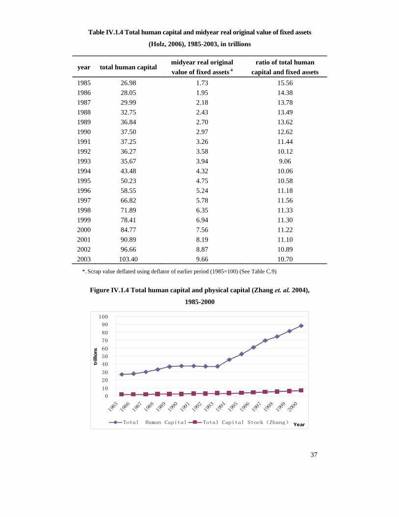
37

Table IV.1.4 Total human capital and midyear real original value of fixed assets

(Holz, 2006), 1985-2003, in trillions

year total human capital midyear real original value of fixed assets a

ratio of total human capital and fixed assets

1985 26.98 1.73 15.56 1986 28.05 1.95 14.38 1987 29.99 2.18 13.78 1988 32.75 2.43 13.49 1989 36.84 2.70 13.62 1990 37.50 2.97 12.62 1991 37.25 3.26 11.44 1992 36.27 3.58 10.12 1993 35.67 3.94 9.06 1994 43.48 4.32 10.06 1995 50.23 4.75 10.58 1996 58.55 5.24 11.18 1997 66.82 5.78 11.56 1998 71.89 6.35 11.33 1999 78.41 6.94 11.30 2000 84.77 7.56 11.22 2001 90.89 8.19 11.10 2002 96.66 8.87 10.89 2003 103.40 9.66 10.70

*. Scrap value deflated using deflator of earlier period (1985=100) (See Table C.9)

Figure IV.1.4 Total human capital and physical capital (Zhang et. al. 2004),

1985-2000

0

10

20

30

40

50

60

70

80

90

100

1985

1986

1987

1988

1989

1990

1991

1992

1993

1994

1995

1996

1997

1998

1999

2000

Year

trillions

Total Human Capital Total Capital Stock（Zhang）

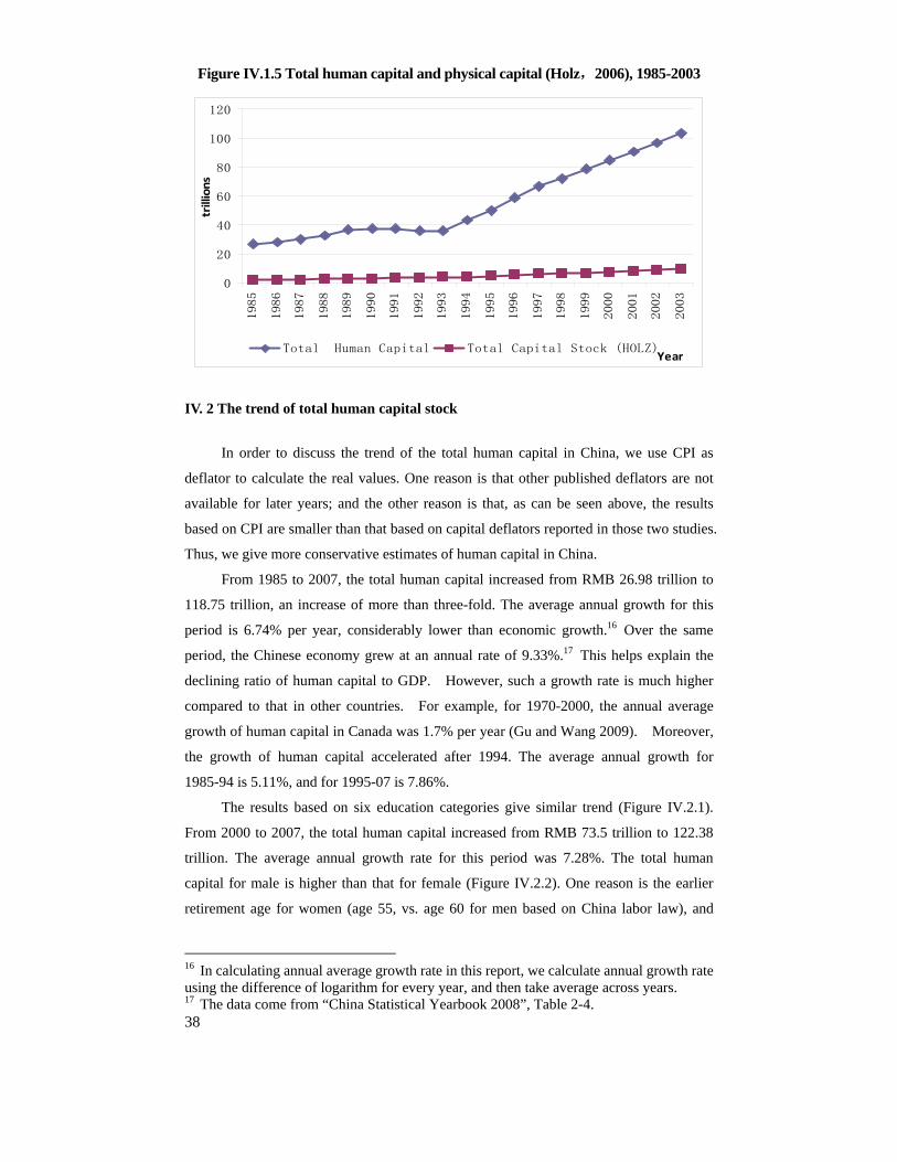
38

Figure IV.1.5 Total human capital and physical capital (Holz，2006), 1985-2003

0

20

40

60

80

100

120

1985

1986

1987

1988

1989

1990

1991

1992

1993

1994

1995

1996

1997

1998

1999

2000

2001

2002

2003

Year

trillions

Total Human Capital Total Capital Stock (HOLZ)

IV. 2 The trend of total human capital stock

In order to discuss the trend of the total human capital in China, we use CPI as

deflator to calculate the real values. One reason is that other published deflators are not

available for later years; and the other reason is that, as can be seen above, the results

based on CPI are smaller than that based on capital deflators reported in those two studies.

Thus, we give more conservative estimates of human capital in China.

From 1985 to 2007, the total human capital increased from RMB 26.98 trillion to

118.75 trillion, an increase of more than three-fold. The average annual growth for this

period is 6.74% per year, considerably lower than economic growth.16 Over the same

period, the Chinese economy grew at an annual rate of 9.33%.17 This helps explain the

declining ratio of human capital to GDP. However, such a growth rate is much higher

compared to that in other countries. For example, for 1970-2000, the annual average

growth of human capital in Canada was 1.7% per year (Gu and Wang 2009). Moreover,

the growth of human capital accelerated after 1994. The average annual growth for

1985-94 is 5.11%, and for 1995-07 is 7.86%.

The results based on six education categories give similar trend (Figure IV.2.1).

From 2000 to 2007, the total human capital increased from RMB 73.5 trillion to 122.38

trillion. The average annual growth rate for this period was 7.28%. The total human

capital for male is higher than that for female (Figure IV.2.2). One reason is the earlier

retirement age for women (age 55, vs. age 60 for men based on China labor law), and

16 In calculating annual average growth rate in this report, we calculate annual growth rate using the difference of logarithm for every year, and then take average across years. 17 The data come from “China Statistical Yearbook 2008”, Table 2-4.

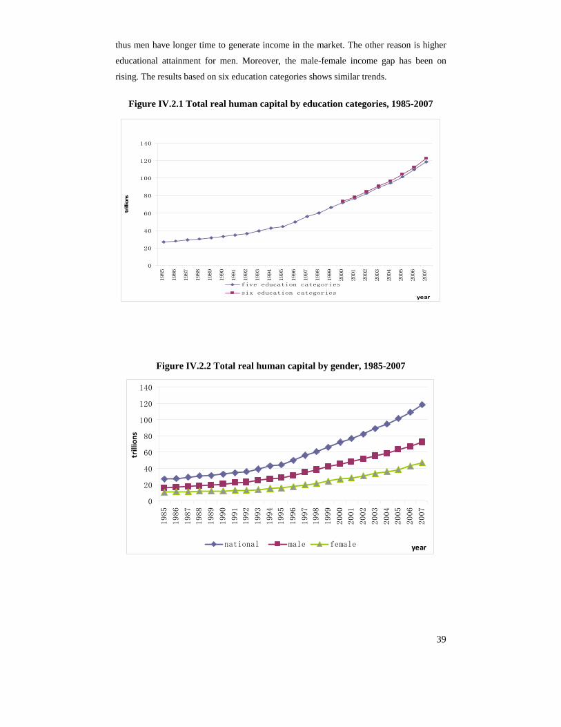
39

thus men have longer time to generate income in the market. The other reason is higher

educational attainment for men. Moreover, the male-female income gap has been on

rising. The results based on six education categories shows similar trends.

Figure IV.2.1 Total real human capital by education categories, 1985-2007

0

20

40

60

80

100

120

140

1985

1986

1987

1988

1989

1990

1991

1992

1993

1994

1995

1996

1997

1998

1999

2000

2001

2002

2003

2004

2005

2006

2007

year

trillions

five education categories

six education categories

Figure IV.2.2 Total real human capital by gender, 1985-2007

0

20

40

60

80

100

120

140

1985

1986

1987

1988

1989

1990

1991

1992

1993

1994

1995

1996

1997

1998

1999

2000

2001

2002

2003

2004

2005

2006

2007

year

trillions

national male female

40

Figure IV.2.3 Total real human capital by urban and rural, 1985-2007

0

20

40

60

80

100

120

140

1985

1986

1987

1988

1989

1990

1991

1992

1993

1994

1995

1996

1997

1998

1999

2000

2001

2002

2003

2004

2005

2006

2007

year

trillions

urban rural national

Figure IV.2.3 shows the total human capital for urban and rural China separately.

Before 1995, the amount of total human capital in both areas was very close. In fact, rural

human capital was even larger than that in the urban area until 1993. Since 1995,

however, the human capital in the urban area has been rising much more rapidly. The

total human capital for the rural area was 16.03 trillion in 1985 and 40.25 trillion in 2007;

and for the urban area it was 10.95 trillion and 78.50 trillion, respectively. In this period,

the annual growth rates of human capital were 4.19% (4.99% after 1995) and 8.95%

(9.90% after 1995) for rural and urban areas, respectively. The urban-rural gap in the

estimated human capital stock increased from 1.24 trillion in 1995 to 38.25 trillion in

2007, growing at an annual rate of 28.55%. Figure IV.2.4 shows the total human capital

estimates in urban and rural areas based on six education categories. The trends are

similar to those based on five education categories.18

18 However, our estimates for the rural area are rather conservative because we assume the same male retirement age of 60 and female retirement age of 55 as in the urban area. In fact, many rural residents continue to work after these ages.

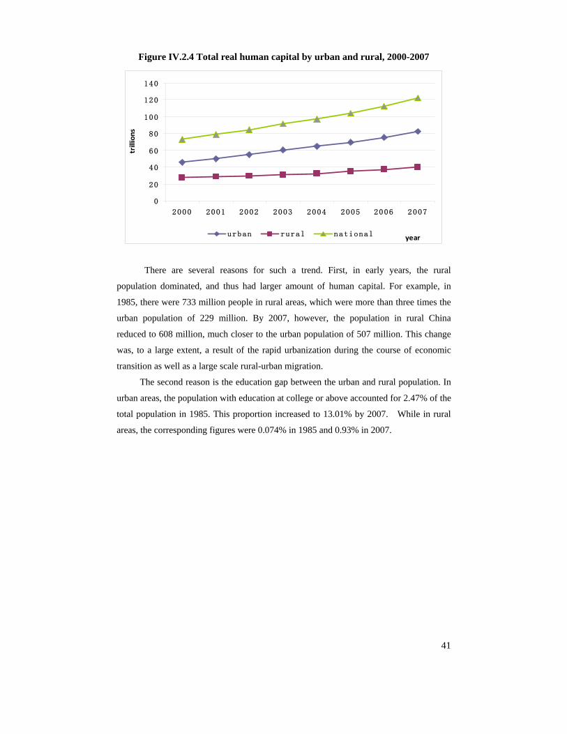
41

Figure IV.2.4 Total real human capital by urban and rural, 2000-2007

0

20

40

60

80

100

120

140

2000 2001 2002 2003 2004 2005 2006 2007

year

trillions

urban rural national

There are several reasons for such a trend. First, in early years, the rural

population dominated, and thus had larger amount of human capital. For example, in

1985, there were 733 million people in rural areas, which were more than three times the

urban population of 229 million. By 2007, however, the population in rural China

reduced to 608 million, much closer to the urban population of 507 million. This change

was, to a large extent, a result of the rapid urbanization during the course of economic

transition as well as a large scale rural-urban migration.

The second reason is the education gap between the urban and rural population. In

urban areas, the population with education at college or above accounted for 2.47% of the

total population in 1985. This proportion increased to 13.01% by 2007. While in rural

areas, the corresponding figures were 0.074% in 1985 and 0.93% in 2007.

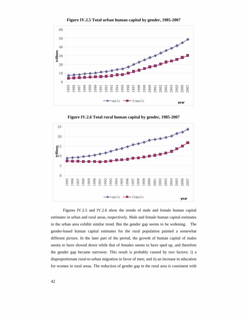
42

Figure IV.2.5 Total urban human capital by gender, 1985-2007

0

10

20

30

40

50

60

1985

1986

1987

1988

1989

1990

1991

1992

1993

1994

1995

1996

1997

1998

1999

2000

2001

2002

2003

2004

2005

2006

2007

year

trillions

male female

Figure IV.2.6 Total rural human capital by gender, 1985-2007

0

5

10

15

20

25

1985

1986

1987

1988

1989

1990

1991

1992

1993

1994

1995

1996

1997

1998

1999

2000

2001

2002

2003

2004

2005

2006

2007

year

trillions

male female

Figures IV.2.5 and IV.2.6 show the trends of male and female human capital

estimates in urban and rural areas, respectively. Male and female human capital estimates

in the urban area exhibit similar trend. But the gender gap seems to be widening. The

gender-based human capital estimates for the rural population painted a somewhat

different picture. In the later part of the period, the growth of human capital of males

seems to have slowed down while that of females seems to have sped up, and therefore

the gender gap became narrower. This result is probably caused by two factors: i) a

disproportionate rural-to-urban migration in favor of men; and ii) an increase in education

for women in rural areas. The reduction of gender gap in the rural area is consistent with

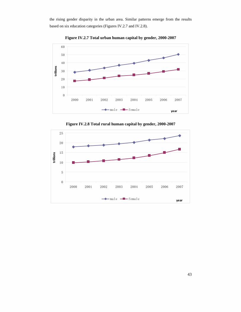
43

the rising gender disparity in the urban area. Similar patterns emerge from the results

based on six education categories (Figures IV.2.7 and IV.2.8).

Figure IV.2.7 Total urban human capital by gender, 2000-2007

0

10

20

30

40

50

60

2000 2001 2002 2003 2004 2005 2006 2007

year

trillions

male female

Figure IV.2.8 Total rural human capital by gender, 2000-2007

0

5

10

15

20

25

2000 2001 2002 2003 2004 2005 2006 2007

year

trillions

male female

44

Table IV.2.1 Total human capital index, 1985-2007 (1985=100)

Year total

human capital

male total human capital

female total

human capital

urban total human capital

rural total human capital

1985 100 100 100 100 100

1986 104 105 102 108 101

1987 109 111 107 118 103

1988 113 118 108 126 105

1989 117 123 110 134 106

1990 122 129 112 143 109

1991 128 138 114 153 111

1992 135 146 120 164 115

1993 146 159 128 181 123

1994 158 171 140 198 131

1995 165 179 145 209 135

1996 184 200 162 245 143

1997 208 225 183 289 152

1998 224 243 197 322 157

1999 246 266 219 367 164

2000 268 288 239 406 173

2001 286 306 256 442 179

2002 306 326 279 484 184

2003 331 348 305 533 192

2004 351 370 324 568 202

2005 377 397 349 611 217

2006 406 421 384 661 232

2007 440 454 420 717 251

Finally we calculate human capital index using 1985 as the base year and set its

value at 100. The results for each group are reported in Table IV.2.1. Figure IV.2.9 shows

the index of total human capital, and Figures IV.2.10 and IV.2.11 show the index by

gender for urban and rural areas, respectively.

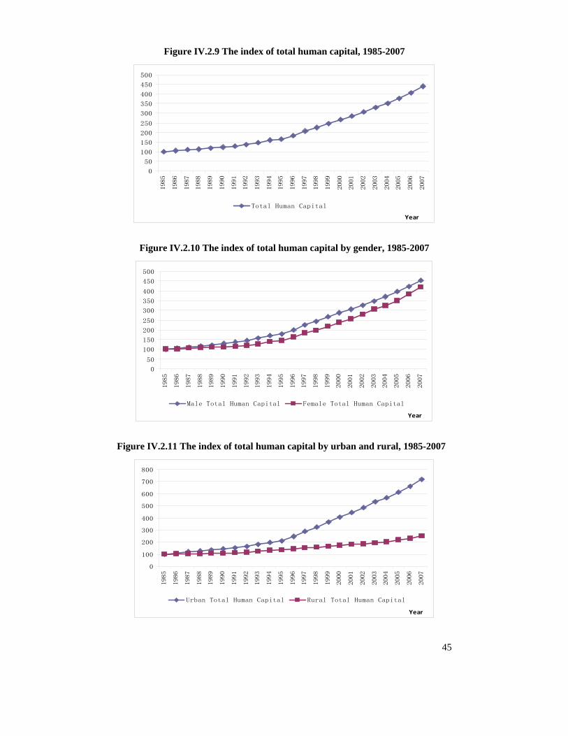
45

Figure IV.2.9 The index of total human capital, 1985-2007

0

50

100

150

200

250

300

350

400

450

500

1985

1986

1987

1988

1989

1990

1991

1992

1993

1994

1995

1996

1997

1998

1999

2000

2001

2002

2003

2004

2005

2006

2007

Year

Total Human Capital

Figure IV.2.10 The index of total human capital by gender, 1985-2007

0

50

100

150

200

250

300

350

400

450

500

1985

1986

1987

1988

1989

1990

1991

1992

1993

1994

1995

1996

1997

1998

1999

2000

2001

2002

2003

2004

2005

2006

2007

Year

Male Total Human Capital Female Total Human Capital

Figure IV.2.11 The index of total human capital by urban and rural, 1985-2007

0

100

200

300

400

500

600

700

800

1985

1986

1987

1988

1989

1990

1991

1992

1993

1994

1995

1996

1997

1998

1999

2000

2001

2002

2003

2004

2005

2006

2007

Year

Urban Total Human Capital Rural Total Human Capital

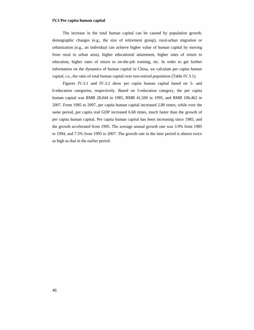
46

IV.3 Per capita human capital

The increase in the total human capital can be caused by population growth,

demographic changes (e.g., the size of retirement group), rural-urban migration or

urbanization (e.g., an individual can achieve higher value of human capital by moving

from rural to urban area), higher educational attainment, higher rates of return to

education, higher rates of return to on-the-job training, etc. In order to get further

information on the dynamics of human capital in China, we calculate per capita human

capital, i.e., the ratio of total human capital over non-retired population (Table IV.3.1).

Figures IV.3.1 and IV.3.2 show per capita human capital based on 5- and

6-education categories, respectively. Based on 5-education category, the per capita

human capital was RMB 28,044 in 1985, RMB 41,500 in 1995, and RMB 106,462 in

2007. From 1985 to 2007, per capita human capital increased 2.80 times; while over the

same period, per capita real GDP increased 6.68 times, much faster than the growth of

per capita human capital. Per capita human capital has been increasing since 1985, and

the growth accelerated from 1995. The average annual growth rate was 3.9% from 1985

to 1994, and 7.5% from 1995 to 2007. The growth rate in the later period is almost twice

as high as that in the earlier period.

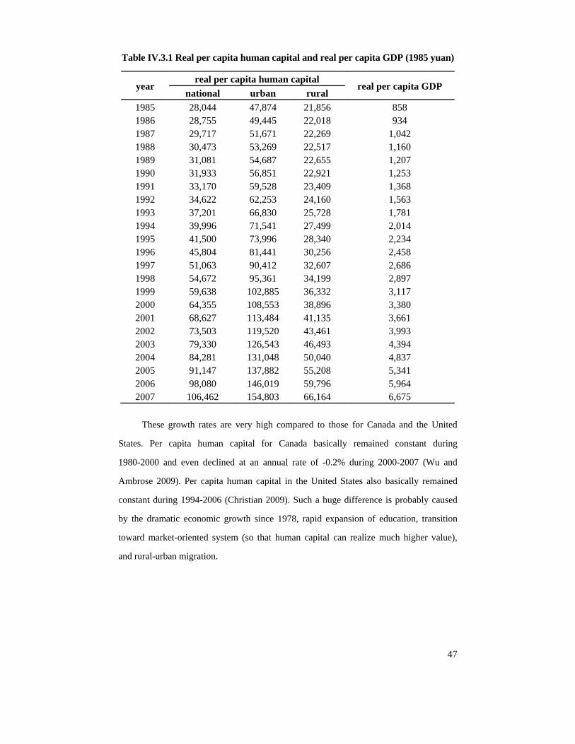
47

Table IV.3.1 Real per capita human capital and real per capita GDP (1985 yuan)

year real per capita human capital

real per capita GDP national urban rural

1985 28,044 47,874 21,856 858 1986 28,755 49,445 22,018 934 1987 29,717 51,671 22,269 1,042 1988 30,473 53,269 22,517 1,160 1989 31,081 54,687 22,655 1,207 1990 31,933 56,851 22,921 1,253 1991 33,170 59,528 23,409 1,368 1992 34,622 62,253 24,160 1,563 1993 37,201 66,830 25,728 1,781 1994 39,996 71,541 27,499 2,014 1995 41,500 73,996 28,340 2,234 1996 45,804 81,441 30,256 2,458 1997 51,063 90,412 32,607 2,686 1998 54,672 95,361 34,199 2,897 1999 59,638 102,885 36,332 3,117 2000 64,355 108,553 38,896 3,380 2001 68,627 113,484 41,135 3,661 2002 73,503 119,520 43,461 3,993 2003 79,330 126,543 46,493 4,394 2004 84,281 131,048 50,040 4,837 2005 91,147 137,882 55,208 5,341 2006 98,080 146,019 59,796 5,964 2007 106,462 154,803 66,164 6,675

These growth rates are very high compared to those for Canada and the United

States. Per capita human capital for Canada basically remained constant during

1980-2000 and even declined at an annual rate of -0.2% during 2000-2007 (Wu and

Ambrose 2009). Per capita human capital in the United States also basically remained

constant during 1994-2006 (Christian 2009). Such a huge difference is probably caused

by the dramatic economic growth since 1978, rapid expansion of education, transition

toward market-oriented system (so that human capital can realize much higher value),

and rural-urban migration.

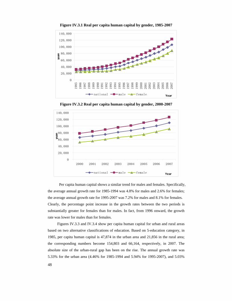
48

Figure IV.3.1 Real per capita human capital by gender, 1985-2007

0

20,000

40,000

60,000

80,000

100,000

120,000

140,000

1985

1986

1987

1988

1989

1990

1991

1992

1993

1994

1995

1996

1997

1998

1999

2000

2001

2002

2003

2004

2005

2006

2007

Year

yuan

national male female

Figure IV.3.2 Real per capita human capital by gender, 2000-2007

0

20,000

40,000

60,000

80,000

100,000

120,000

140,000

2000 2001 2002 2003 2004 2005 2006 2007

Year

yuan

national male female

Per capita human capital shows a similar trend for males and females. Specifically,

the average annual growth rate for 1985-1994 was 4.8% for males and 2.6% for females;

the average annual growth rate for 1995-2007 was 7.2% for males and 8.1% for females.

Clearly, the percentage point increase in the growth rates between the two periods is

substantially greater for females than for males. In fact, from 1996 onward, the growth

rate was lower for males than for females.

Figures IV.3.3 and IV.3.4 show per capita human capital for urban and rural areas

based on two alternative classifications of education. Based on 5-education category, in

1985, per capita human capital is 47,874 in the urban area and 21,856 in the rural area;

the corresponding numbers become 154,803 and 66,164, respectively, in 2007. The

absolute size of the urban-rural gap has been on the rise. The annual growth rate was

5.33% for the urban area (4.46% for 1985-1994 and 5.94% for 1995-2007), and 5.03%

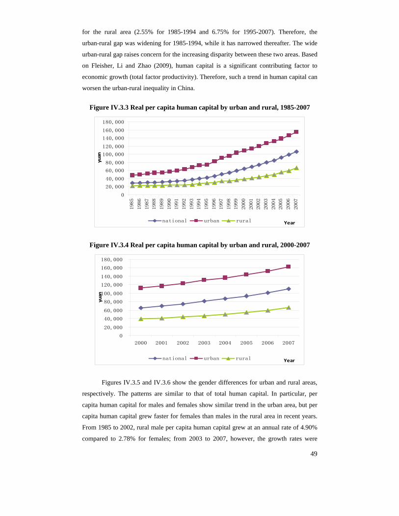
49

for the rural area (2.55% for 1985-1994 and 6.75% for 1995-2007). Therefore, the

urban-rural gap was widening for 1985-1994, while it has narrowed thereafter. The wide

urban-rural gap raises concern for the increasing disparity between these two areas. Based

on Fleisher, Li and Zhao (2009), human capital is a significant contributing factor to

economic growth (total factor productivity). Therefore, such a trend in human capital can

worsen the urban-rural inequality in China.

Figure IV.3.3 Real per capita human capital by urban and rural, 1985-2007

0

20,000

40,000

60,000

80,000

100,000

120,000

140,000

160,000

180,000

1985

1986

1987

1988

1989

1990

1991

1992

1993

1994

1995

1996

1997

1998

1999

2000

2001

2002

2003

2004

2005

2006

2007

Year

yuan

national urban rural

Figure IV.3.4 Real per capita human capital by urban and rural, 2000-2007

0

20,000

40,000

60,000

80,000

100,000

120,000

140,000

160,000

180,000

2000 2001 2002 2003 2004 2005 2006 2007

Year

yuan

national urban rural

Figures IV.3.5 and IV.3.6 show the gender differences for urban and rural areas,

respectively. The patterns are similar to that of total human capital. In particular, per

capita human capital for males and females show similar trend in the urban area, but per

capita human capital grew faster for females than males in the rural area in recent years.

From 1985 to 2002, rural male per capita human capital grew at an annual rate of 4.90%

compared to 2.78% for females; from 2003 to 2007, however, the growth rates were

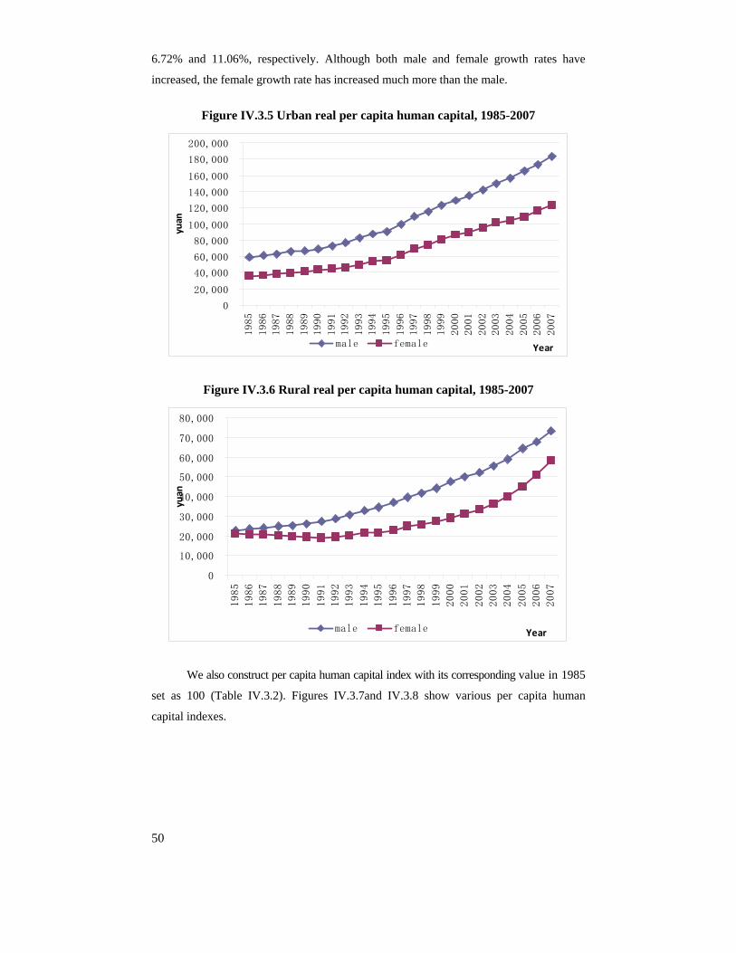
50

6.72% and 11.06%, respectively. Although both male and female growth rates have

increased, the female growth rate has increased much more than the male.

Figure IV.3.5 Urban real per capita human capital, 1985-2007

0

20,000

40,000

60,000

80,000

100,000

120,000

140,000

160,000

180,000

200,000

1985

1986

1987

1988

1989

1990

1991

1992

1993

1994

1995

1996

1997

1998

1999

2000

2001

2002

2003

2004

2005

2006

2007

Year

yuan

male female

Figure IV.3.6 Rural real per capita human capital, 1985-2007

0

10,000

20,000

30,000

40,000

50,000

60,000

70,000

80,000

1985

1986

1987

1988

1989

1990

1991

1992

1993

1994

1995

1996

1997

1998

1999

2000

2001

2002

2003

2004

2005

2006

2007

Year

yuan

male female

We also construct per capita human capital index with its corresponding value in 1985

set as 100 (Table IV.3.2). Figures IV.3.7and IV.3.8 show various per capita human

capital indexes.

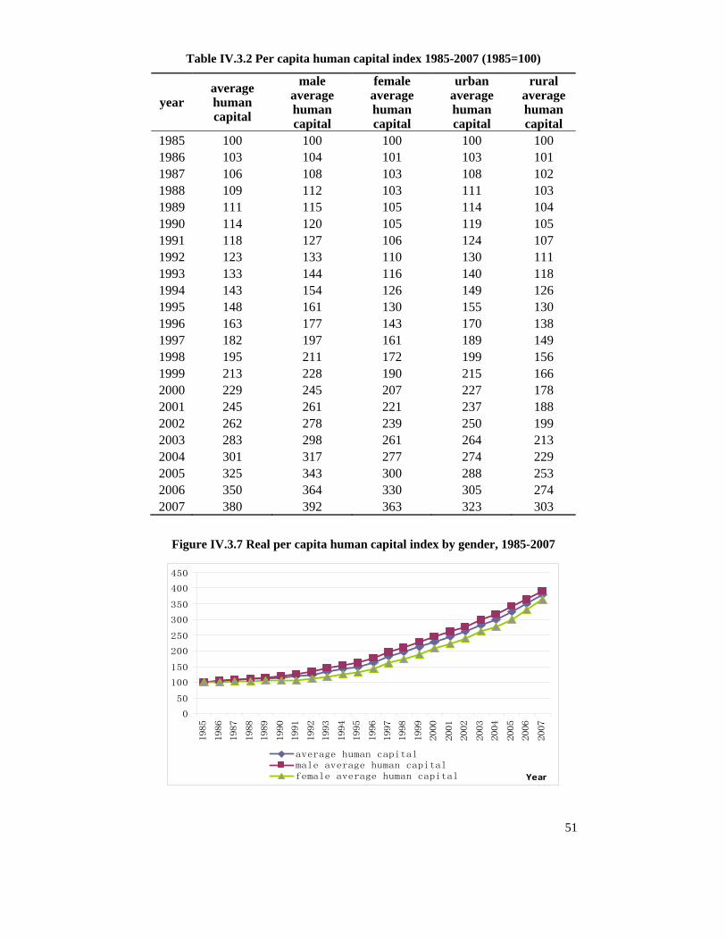
51

Table IV.3.2 Per capita human capital index 1985-2007 (1985=100)

year average human capital

male average human capital

female average human capital

urban average human capital

rural average human capital

1985 100 100 100 100 100 1986 103 104 101 103 101 1987 106 108 103 108 102 1988 109 112 103 111 103 1989 111 115 105 114 104 1990 114 120 105 119 105 1991 118 127 106 124 107 1992 123 133 110 130 111 1993 133 144 116 140 118 1994 143 154 126 149 126 1995 148 161 130 155 130 1996 163 177 143 170 138 1997 182 197 161 189 149 1998 195 211 172 199 156 1999 213 228 190 215 166 2000 229 245 207 227 178 2001 245 261 221 237 188 2002 262 278 239 250 199 2003 283 298 261 264 213 2004 301 317 277 274 229 2005 325 343 300 288 253 2006 350 364 330 305 274 2007 380 392 363 323 303

Figure IV.3.7 Real per capita human capital index by gender, 1985-2007

0

50

100

150

200

250

300

350

400

450

1985

1986

1987

1988

1989

1990

1991

1992

1993

1994

1995

1996

1997

1998

1999

2000

2001

2002

2003

2004

2005

2006

2007

Year

average human capitalmale average human capitalfemale average human capital

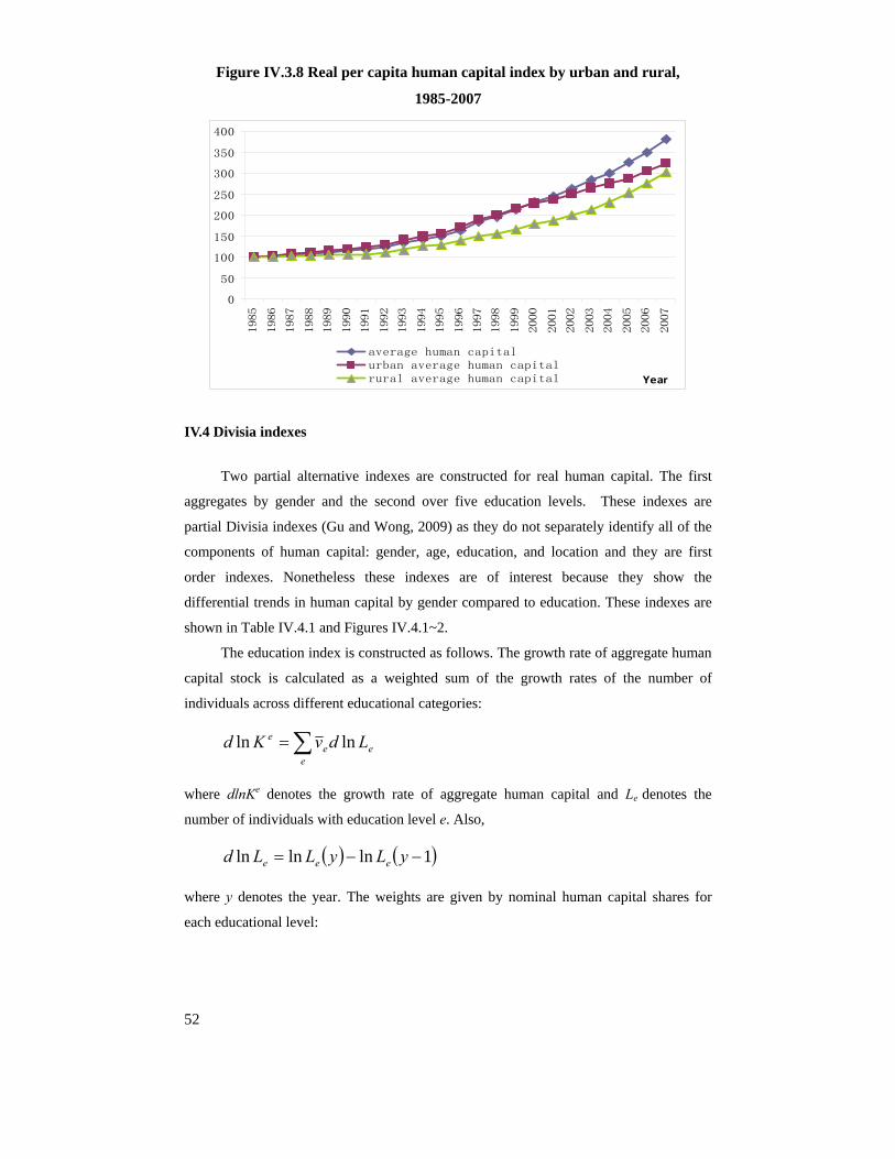
52

Figure IV.3.8 Real per capita human capital index by urban and rural,

1985-2007

0

50

100

150

200

250

300

350

400

1985

1986

1987

1988

1989

1990

1991

1992

1993

1994

1995

1996

1997

1998

1999

2000

2001

2002

2003

2004

2005

2006

2007

Year

average human capitalurban average human capitalrural average human capital

IV.4 Divisia indexes

Two partial alternative indexes are constructed for real human capital. The first

aggregates by gender and the second over five education levels. These indexes are

partial Divisia indexes (Gu and Wong, 2009) as they do not separately identify all of the

components of human capital: gender, age, education, and location and they are first

order indexes. Nonetheless these indexes are of interest because they show the

differential trends in human capital by gender compared to education. These indexes are

shown in Table IV.4.1 and Figures IV.4.1~2.

The education index is constructed as follows. The growth rate of aggregate human

capital stock is calculated as a weighted sum of the growth rates of the number of

individuals across different educational categories:

ee

ee LdvKd lnln ∑=

where dlnKe denotes the growth rate of aggregate human capital and Le denotes the

number of individuals with education level e. Also,

( ) ( )1lnlnln −−= yLyLLd eee

where y denotes the year. The weights are given by nominal human capital shares for

each educational level:

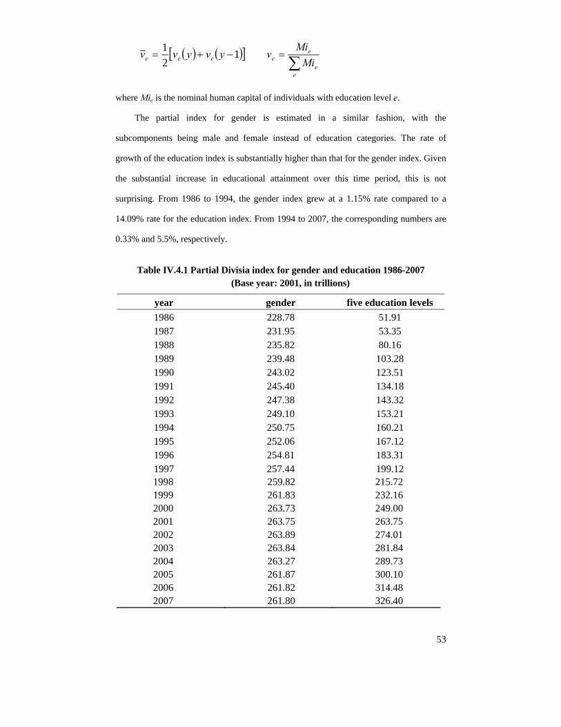
53

( ) ( )[ ]121

−+= yvyvv eee ∑

=

ee

ee Mi

Miv

where Mie is the nominal human capital of individuals with education level e.

The partial index for gender is estimated in a similar fashion, with the

subcomponents being male and female instead of education categories. The rate of

growth of the education index is substantially higher than that for the gender index. Given

the substantial increase in educational attainment over this time period, this is not

surprising. From 1986 to 1994, the gender index grew at a 1.15% rate compared to a

14.09% rate for the education index. From 1994 to 2007, the corresponding numbers are

0.33% and 5.5%, respectively.

Table IV.4.1 Partial Divisia index for gender and education 1986-2007 (Base year: 2001, in trillions)

year gender five education levels 1986 228.78 51.91 1987 231.95 53.35 1988 235.82 80.16 1989 239.48 103.28 1990 243.02 123.51 1991 245.40 134.18 1992 247.38 143.32 1993 249.10 153.21 1994 250.75 160.21 1995 252.06 167.12 1996 254.81 183.31 1997 257.44 199.12 1998 259.82 215.72 1999 261.83 232.16 2000 263.73 249.00 2001 263.75 263.75 2002 263.89 274.01 2003 263.84 281.84 2004 263.27 289.73 2005 261.87 300.10 2006 261.82 314.48 2007 261.80 326.40

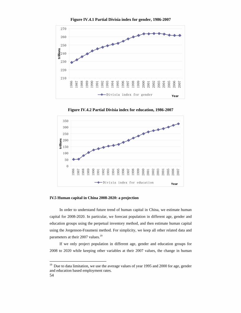
54

Figure IV.4.1 Partial Divisia index for gender, 1986-2007

210

220

230

240

250

260

270

1986

1987

1988

1989

1990

1991

1992

1993

1994

1995

1996

1997

1998

1999

2000

2001

2002

2003

2004

2005

2006

2007

Year

trillions

Divisia index for gender

Figure IV.4.2 Partial Divisia index for education, 1986-2007

0

50

100

150

200

250

300

350

1986

1987

1988

1989

1990

1991

1992

1993

1994

1995

1996

1997

1998

1999

2000

2001

2002

2003

2004

2005

2006

2007

Year

trillions

Divisia index for education

IV.5 Human capital in China 2008-2020: a projection

In order to understand future trend of human capital in China, we estimate human

capital for 2008-2020. In particular, we forecast population in different age, gender and

education groups using the perpetual inventory method, and then estimate human capital

using the Jorgenson-Fraumeni method. For simplicity, we keep all other related data and

parameters at their 2007 values.19

If we only project population in different age, gender and education groups for

2008 to 2020 while keeping other variables at their 2007 values, the change in human

19 Due to data limitation, we use the average values of year 1995 and 2000 for age, gender and education based employment rates.

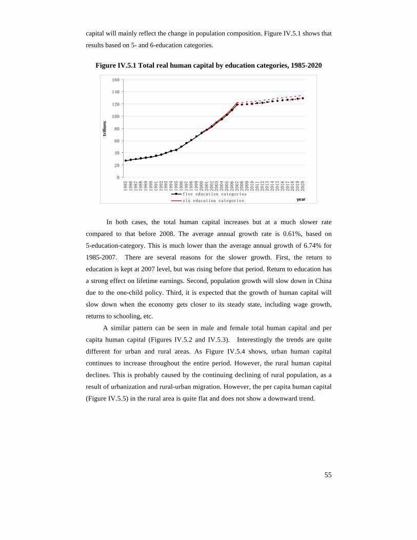
55

capital will mainly reflect the change in population composition. Figure IV.5.1 shows that

results based on 5- and 6-education categories.

Figure IV.5.1 Total real human capital by education categories, 1985-2020

0

20

40

60

80

100

120

140

160

1985

1986

1987

1988

1989

1990

1991

1992

1993

1994

1995

1996

1997

1998

1999

2000

2001

2002

2003

2004

2005

2006

2007

2008

2009

2010

2011

2012

2013

2014

2015

2016

2017

2018

2019

2020

year

trillions

five education categories

six education categories

In both cases, the total human capital increases but at a much slower rate

compared to that before 2008. The average annual growth rate is 0.61%, based on

5-education-category. This is much lower than the average annual growth of 6.74% for

1985-2007. There are several reasons for the slower growth. First, the return to

education is kept at 2007 level, but was rising before that period. Return to education has

a strong effect on lifetime earnings. Second, population growth will slow down in China

due to the one-child policy. Third, it is expected that the growth of human capital will

slow down when the economy gets closer to its steady state, including wage growth,

returns to schooling, etc.

A similar pattern can be seen in male and female total human capital and per

capita human capital (Figures IV.5.2 and IV.5.3). Interestingly the trends are quite

different for urban and rural areas. As Figure IV.5.4 shows, urban human capital

continues to increase throughout the entire period. However, the rural human capital

declines. This is probably caused by the continuing declining of rural population, as a

result of urbanization and rural-urban migration. However, the per capita human capital

(Figure IV.5.5) in the rural area is quite flat and does not show a downward trend.

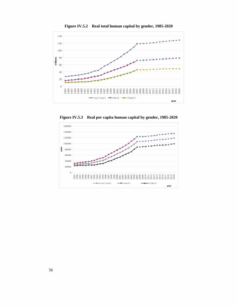
56

Figure IV.5.2 Real total human capital by gender, 1985-2020

0

20

40

60

80

100

120

140

1985

1986

1987

1988

1989

1990

1991

1992

1993

1994

1995

1996

1997

1998

1999

2000

2001

2002

2003

2004

2005

2006

2007

2008

2009

2010

2011

2012

2013

2014

2015

2016

2017

2018

2019

2020

year

trillions

national male female

Figure IV.5.3 Real per capita human capital by gender, 1985-2020

0

20000

40000

60000

80000

100000

120000

140000

160000

1985

1986

1987

1988

1989

1990

1991

1992

1993

1994

1995

1996

1997

1998

1999

2000

2001

2002

2003

2004

2005

2006

2007

2008

2009

2010

2011

2012

2013

2014

2015

2016

2017

2018

2019

2020

year

yuan

national male female

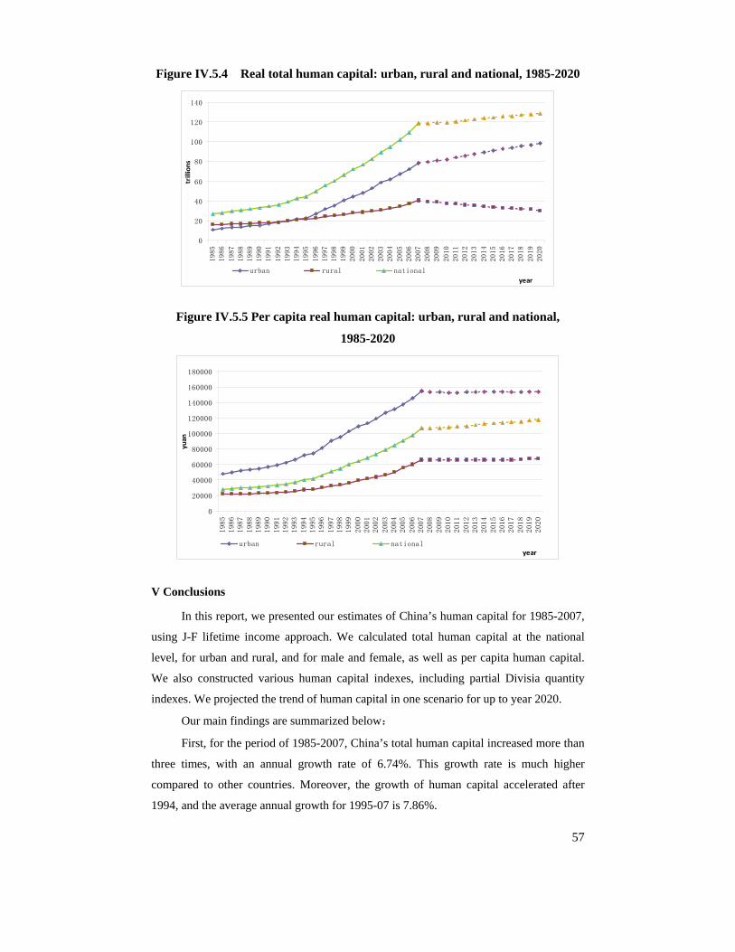
57

Figure IV.5.4 Real total human capital: urban, rural and national, 1985-2020

0

20

40

60

80

100

120

140

1985

1986

1987

1988

1989

1990

1991

1992

1993

1994

1995

1996

1997

1998

1999

2000

2001

2002

2003

2004

2005

2006

2007

2008

2009

2010

2011

2012

2013

2014

2015

2016

2017

2018

2019

2020

year

trillions

urban rural national

Figure IV.5.5 Per capita real human capital: urban, rural and national,

1985-2020

0

20000

40000

60000

80000

100000

120000

140000

160000

180000

1985

1986

1987

1988

1989

1990

1991

1992

1993

1994

1995

1996

1997

1998

1999

2000

2001

2002

2003

2004

2005

2006

2007

2008

2009

2010

2011

2012

2013

2014

2015

2016

2017

2018

2019

2020

year

yuan

urban rural national

V Conclusions

In this report, we presented our estimates of China’s human capital for 1985-2007,

using J-F lifetime income approach. We calculated total human capital at the national

level, for urban and rural, and for male and female, as well as per capita human capital.

We also constructed various human capital indexes, including partial Divisia quantity

indexes. We projected the trend of human capital in one scenario for up to year 2020.

Our main findings are summarized below：

First, for the period of 1985-2007, China’s total human capital increased more than

three times, with an annual growth rate of 6.74%. This growth rate is much higher

compared to other countries. Moreover, the growth of human capital accelerated after

1994, and the average annual growth for 1995-07 is 7.86%.

58

Second, the total human capital in urban area increased at a much higher rate than

in rural area over the period 1985-07. The annual average growth rates are 8.95% and

4.19% respectively for urban and rural areas. The total human capital in urban area

surpassed that in rural area in 1993. The urban-rural gap has been widening rapidly,

probably because of urbanization, large-scale rural-urban migration, and increase in

educational attainment.

Third, per capita human capital also increased rapidly from 1985-2007, with a

higher growth rate since 1995. Interestingly, before 1995 total human capital increased

faster than per capita human capital on average, while since 1995, both have grown at a

similar average annual rate. This result indicates that in recent years, the growth of

human capital is mostly driven by factors such as increases in educational attainment, not

by population growth.

Fourth, the gender gap in total human capital has been widening at the national

level. However, the gender difference in per capita human capital appears to be

narrowing down.

Fifth, the partially education-based human capital index grew at a much higher rate

than the gender-based index. This indicates the greater impact of education on China’s

human capital accumulation.

On the other hand, our results also show that, compared to GDP and physical

capital, human capital grew at a slower pace. More specifically, the ratio of human capital

to GDP decreased from approximately 30 in 1985 to 18 in 2007; and the ratio of human

capital to physical capital also declined from 16-19 in 1985 to 11~12 in 2003, these

findings indicates that the Chinese government should invest more in human capital,

especially compared to physical capital investment.

The gap in total human capital and per capita human capital between urban and

rural areas has been increasing. Thus, in order to reduce urban-rural inequality, more

investment in human capital should be directed to the rural area.

Finally, our projection to 2020 shows that, if we keep everything else at the 2007

level and only allow population to change, the growth of total human capital and per

capita human capital will slow down after 2007. The amount of total human capital will

even decline in rural China. Therefore, more active policies on human capital

investment should be adopted in order to maintain the high speed growth.

Our future work includes: i) finding more data to improve estimates of lifetime

earnings and other related variables; ii) refining the estimation of some related parameters

and data; and iii) refining our projections of future incomes and testing the effects of

various policy scenarios on human capital accumulation.

59

Reference List

Abraham, Katharine (2005), Beyond the Market: Designing Nonmarket Accounts for

the United States, National Academies Press, Washington, D.C.

Ahlroth, Sofia, A. and Bjorklund, A. Forslund (1997), “The Output of the Swedish

Education Sector”, Review of Income and Wealth Volume 43, Number 1, pp.89-104.

Ashenfelter, Orley and Krueger, Alan (1994), “Estimates of the Economic Return to

Schooling from a New Sample of Twins”, American Economic Review 84, December,

pp.1157-73.

Becker, G. (1964), Human Capital, 2nd edition, Columbia University Press, New

York.

Bureau of Statistics of China (2008), China Population Statistical Yearbook 2008,

China Statistics Press, Beijing.

Cai Fang and Wang,Dewen(1999), ”The Sustainability of China's Economic Growth

and Labor Contributions”, Economic Research (Chinese) 10, pp.62-68

Christian, Michael S. (2009), “Human Capital Accounting in the United States: 1994 to

2006”, paper presented at the Canadian Economic Association Annual Conference, May

29.

Coleman, J. (1990), Foundations of Social Theory, Belknap, 304

Démurger, Sylvie (2001), “Infrastructure Development and Economic Growth: An

Explanation for Regional Disparities in China?” Journal of Comparative Economics 19,

pp.95-117.

Ederer, Peer (2006). “Innovation at Work: The European Human Capital Index”, The

Lisbon Council Policy Brief, in conjunction with Deutschland Denken! and Zeppelin

University, Brussels, October 12

Ederer, Peer, Philipp Schuller, and Stepham Willms (2007), “Innovation at work：The

European Human Capital Index”, The Lisbon Council Policy Brief, Volume 2, Number 3,

Brussels

Fleisher, Belton., and Chen, Jian (1997), “The Coast-Noncoast Income Gap,

Productivity and Regional Economic Policy in China”, Journal of Comparative

Economics 252: pp.220-236.

Fleisher, Belton., Sabirianova, Klara., and Wang, Xiaojun (2005), “Returns to Skills

and the Speed of Reforms: Evidence from Central and Eastern Europe, China, and

Russia.”, Journal of Comparative Economics 33, issue 2, pp.351-370.

60

Fleisher, Belton and Wang, Xiaojun (2004), “Skill Differentials, Return to Schooling,

and Market Segmentation in a Transition Economy: the Case of Mainland China”,

Journal of Development Economics 73, pp.315-328.

Fleisher, Belton, Li Haizheng and Zhao Minqiang (2009), “Human Capital, Economic

Growth, and Regional Inequality in China”, Journal of Development Economics,

forthcoming.

Fraumeni, Barbara M. (2006), “A Human Capital Approach to Measuring Government

Education Output”, presentation at the OECD/ONS/Government of Norway Workshop

on the Measurement of Non-market Output and Health, London, England, UK, October

4.

Fraumeni, Barbara M. (2008a), “Human Capital and Investment in Education: A

Streamlined Approach”, presentation at the Fondazione Giovanni Agnelli/OECD

Workshop on the Measurement of Human Capital, Turin, Italy, November 3.

Fraumeni, Barbara M. (2008b), “Human Capital: From Indicators and Indexes to

Accounts,” paper presented at the Fondazione Giovanni Agnelli/OECD Workshop on the

Measurement of Human Capital, Turin, Italy, November 4.

Fraumeni, Barbara M. (2009), “Further Comments: Results by Country and Future

Efforts” presentation at a China Center for Human Capital and Labor Market Research

seminar at the Central University of Finance and Economics, Beijing, China, June 19.

Greaker, Mads and Liu, Gang (2008) “Measuring the Stock of Human Capital for

Norway: A Lifetime Labour Income Approach,” paper presented at the Fondazione

Giovanni Agnelli/OECD Workshop on the Measurement of Human Capital, Turin, Italy,

November 3.

Griliches, Zvi, “Estimating the Returns to Schooling.” Econometrica 45, 1977,

pp.1-22.

Gu, Wulong and Wong, Ambrose (2008), “Human Development and its Contribution

to the Wealth Accounts in Canada,” paper presented at the Fondazione Giovanni

Agnelli/OECD Workshop on the Measurement of Human Capital, Turin, Italy, November

3.

Gu, Wulong and Wong Ambrose (2009), “Human Development and its Contribution to

the Wealth Accounts in Canada,” paper presented at the Canadian Economic Association

Annual Conference, May 29.

Heckman, James J. (2005), “China's Human Capital Investment”, China Economic

Review 16, pp.50-70.

61

Holz, Carsten A. (2006), “New Capital Estimates for China”, China Economic Review

17, pp.142-185.

Hou,Yafei and Cao Yin(2000), ”Analysis of the Quality of Human Capital Stock”,

Chinese Journal of Population Science(Chinese) 6, pp.43-48

Hu,Angang(2002), ”From the Most Populous Country to A Country with Great Power

of Human Capital:1980-2000”, Chinese Journal of Population Science(Chinese) 5,

pp.1-10

Hu,Yongyuan(2005), ”Human Capital and Economic Growth: A Co-integration

Analysis”, Science and Technology Management Research(Chinese) 4, pp.88-90

Jorgenson, Dale W. and Fraumeni, Barbara M. (1989), “The Accumulation of Human

and Non-Human Capital, 1948-1984,” in R. Lipsey and H. Tice eds., The Measurement of

Saving, Investment and Wealth, Chicago, University of Chicago Press, NBER, pp.

227-282.

Jorgenson, Dale W. and Fraumeni, Barbara M. (1992a), “Investment in Education and

U.S. Economic Growth,” Scandinavian Journal of Economics, Vol. 94, supplement, pp.

S51-70.

Jorgenson, Dale W. and Fraumeni, Barbara M. (1992b), “The Output of the Education

Sector,” in Z. Griliches, T. Breshnahan, M. Manser, and E. Berndt eds., The Output of the

Service Sector, Chicago, NBER, 1992, pp. 303-341.

Keeley, Brian (2007), Human Capital, How What You Know Shapes Your Life, OECD

Insights, Paris.

Kendrick, J. (1976), The Formation and Stocks of Total Capital, NBER, Columbia

University Press, New York, N.Y.

Koman, R., and Marin, D. (1997), “Human Capital and Macroeconomic Growth:

Austria and Germany 1960-1997. An Update.” IAS Economics Series No. 69.

Laroche, M. and Merette, M. (2000), “Measuring Human Capital in Canada.” Ministry

of Finance of Canada.

Le, Trinh Van Thi, Gibson, John, and Oxley, Les (2005), “Measuring the Stock of

Human Capital in New Zealand,” Mathematics and Computers in Simulation, Volume

68, Issue 5-6, May, pp. 485-98.

Le, Trinh, Gibson, John, and Oxley, Les (2003), “Cost- and Income-Based Measures

of Human Capital.” Journal of Economic Surveys 17, 3: pp.271-307.

Le, Trinh, Gibson, John, and Oxley, Les (2005), “Measures of Human Capital: A

Review of the Literature.” New Zealand Treasury Working Paper 05/10.

62

Li, Haizheng (2003), “Economic Transition and Returns to Education in China.”

Economics of Education Review 2 317-328.

Liu, Zhiqiang (1998), “Earnings, Education, and Economic Reforms in Urban China.”

Economic Development and Cultural Change 46, pp.697-725.

Liu, Zhiqiang (2007), "The External Returns to Education: Evidence from Chinese

Cities”, Journal of Urban Economics 61 (3), pp.542-564.

Maurer-Fazio, Maggie (1999), “Earnings and Education in China’s Transition to a

Market Economy: Survey Evidence from 1989 and 1992.” China Economic Review 10,

pp.17-40.

Mincer, Jacob (1974), Schooling, Experience and Earnings. Columbia University Press.

New York.

Mulligan, C. B., and Sala-i-Martin, X. (1997), “A Labor Income-based Measure of the

Value of Human Capital: An Application to the States of the United States”. Japan and

the World Economy 9, 2: pp.159-191.

OECD (2001), The Well-being of Nations: The Role of Human and Social Capital,

OECD, Paris.

Qian,Xuya, and Liu,Jie(2007), ”Empirical Study of Human Capital in China”, Statistic

Research(Chinese) 3, pp.39-45

Schultz, T. (1961), “Investment in Human Capital”, American Economic Review 51, 1:

pp.1-17.

Stroombergen, A., D. Rose and Nana, G. (2002), “Review of the Statistical

Measurement of Human Capital”, Statistics New Zealand working paper.

Wang,Dejin and Xiang,Rongmei(2006), ”Estimates of Human Capital Stock in

China”,Statistics and Decision (Chinese) 5, pp.100-102

Wang, Xiaojun, Fleisher, Belton, Li, Haizheng, and Li, Shi (2009) “Access to Higher

Education and Inequality: A Chinese Experiment.” IZA Discussion Paper No. 2823.

Wei, Hui (2008) “Developments in the Estimation of the Value of Human Capital in

Australia,” paper presented at the Fondazione Giovanni Agnelli/OECD Workshop on the

Measurement of Human Capital, Turin, Italy, November 3.

World Bank (1997), “Expanding the Measure of Wealth: Indicators of

Environmentally Sustainable Development,” Environmentally Sustainable Development

Studies and Monographs Series No. 17, Washington, D.C.

World Bank (2006) Where is the Wealth of Nations, Measuring Capital for the 21st

Century, The International Bank for Reconstruction and Development/The World Bank,

Washington, DC.

63

Yang, Dennis (2005), “Determinants of Schooling Returns during Transition: Evidence

from Chinese Cities.” Journal of Comparative Economics 33, pp.244-264.

Yu,Shujing(2008), ”Comprehensive Evaluation and Dynamic Analysis on China's

Provincial-level Regional Human Capital”, Modern Management Science(Chinese) 4, pp.

36-37

Zhang Fan(2000), ”Estimates of Physical Capital and Human Capital in China”,

Economic Research (Chinese) 8, pp.66-71

Zhang Jun, Wu, Guiying, and Zhang Jipeng (2004), “Compilation of China’s

Provincial Capital Stock Series Using Perpetual Inventory Method, 1952-2000”,

Economic Research (Chinese), October.

Zhang, Junsen, Zhao, Yaohui, Park, Alberb, and Song, Xiaoqing (2005), “Economic

Returns to Schooling in Urban China, 1988-2001.” Journal of Comparative Economics 33,

pp.730-752.

Zhou,Delu,(2005), ”Population-based Indicators of Human Capital Accounting Theory

and Empirical Study”, Chinese Journal of Population Science(Chinese) 3, pp. 56-62

Zhou Ya(2004), “Study on the Distribution Differences of China's Human Capital”,

Education & Economics(Chinese) 2, pp.17-20

Zhu,Pingfang, and Xu,Dafeng(2007), ”Estimation of Human Capital in Chinese Cities”,

Economic Research (Chinese) 8, pp.84-95

64

Acknowledgement

This research project and international symposium have benefited tremendously

from supports inside and outside the Central University of Finance and Economics

(CUFE). President Guangqian Wang of CUFE supported the project from the very

beginning, and encouraged us to finish the preliminary study ahead of the schedule. Vice

President Junsheng Li, President Assistant Lifen Zhao, and Director of Research Office

Baowen Sun coordinated with various departments and facilitated the project and the

symposium. Many offices in the university, such as the President’s Office, Office of

Research, Assets Management Office, Finance Office, Human Resources Office, and

International Cooperation Office, cooperated to help the CHLR’s research endeavor.

Office spaces, conference facilities and computer labs were generously provided by the

university Virtual Experiment Lab, the School of International Exchange, the Academy

of Public Finance and Policy, and the School of Marxism Studies. The School of

Economics at Georgia Institute of Technology, especially the Chair, Professor Patrick

McCarthy, also generally supported the project. Last but not least, we greatly appreciate

the help from two academic journals -- Economic Research and Labor Economics and

Relations.