Embed Size (px)
Citation preview
Human Pose Regression with Residual Log-likelihood Estimation
Jiefeng Li1 Siyuan Bian1 Ailing Zeng2 Can Wang3
Bo Pang1 Wentao Liu3 Cewu Lu1
1Shanghai Jiao Tong University 2The Chinese University of Hong Kong 3SenseTime Research
Abstract
Heatmap-based methods dominate in the field of hu-man pose estimation by modelling the output distribu-tion through likelihood heatmaps. In contrast, regression-based methods are more efficient but suffer from inferiorperformance. In this work, we explore maximum likeli-hood estimation (MLE) to develop an efficient and effec-tive regression-based methods. From the perspective ofMLE, adopting different regression losses is making differ-ent assumptions about the output density function. A den-sity function closer to the true distribution leads to a bet-ter regression performance. In light of this, we proposea novel regression paradigm with Residual Log-likelihoodEstimation (RLE) to capture the underlying output distri-bution. Concretely, RLE learns the change of the distri-bution instead of the unreferenced underlying distributionto facilitate the training process. With the proposed repa-rameterization design, our method is compatible with off-the-shelf flow models. The proposed method is effective,efficient and flexible. We show its potential in various hu-man pose estimation tasks with comprehensive experiments.Compared to the conventional regression paradigm, regres-sion with RLE bring 12.4 mAP improvement on MSCOCOwithout any test-time overhead. Moreover, for the firsttime, especially on multi-person pose estimation, our re-gression method is superior to the heatmap-based methods.Our code is available at https://github.com/Jeff-sjtu/res-loglikelihood-regression.
1. IntroductionHuman pose estimation has been extensively studied
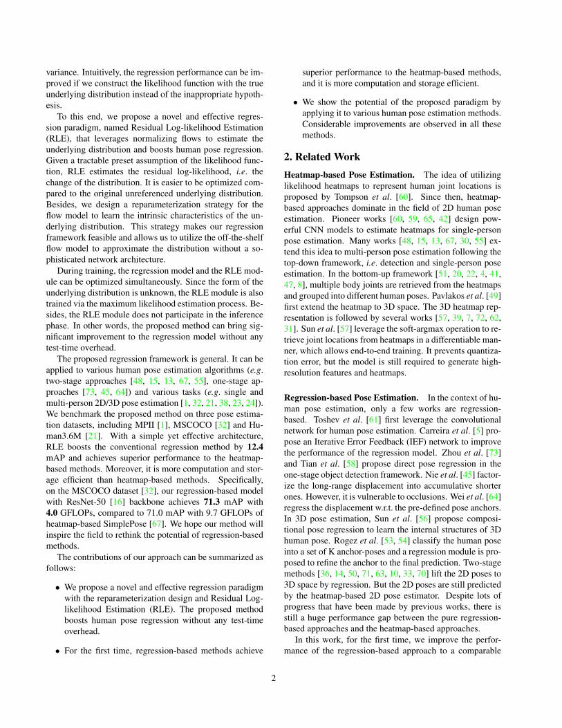
in the area of computer vision [23, 24, 1, 32, 21]. Re-cently, with deep convolutional neural networks, significantprogress has been achieved. Existing methods can be di-vided into two categories: heatmap-based [60, 59, 65, 4,67, 57, 49, 55] and regression-based [61, 5, 56, 73, 45, 64].Heatmap-based methods are dominant in the field of hu-man pose estimation. These methods generate a likelihoodheatmap for each joint and locate the joint as the point
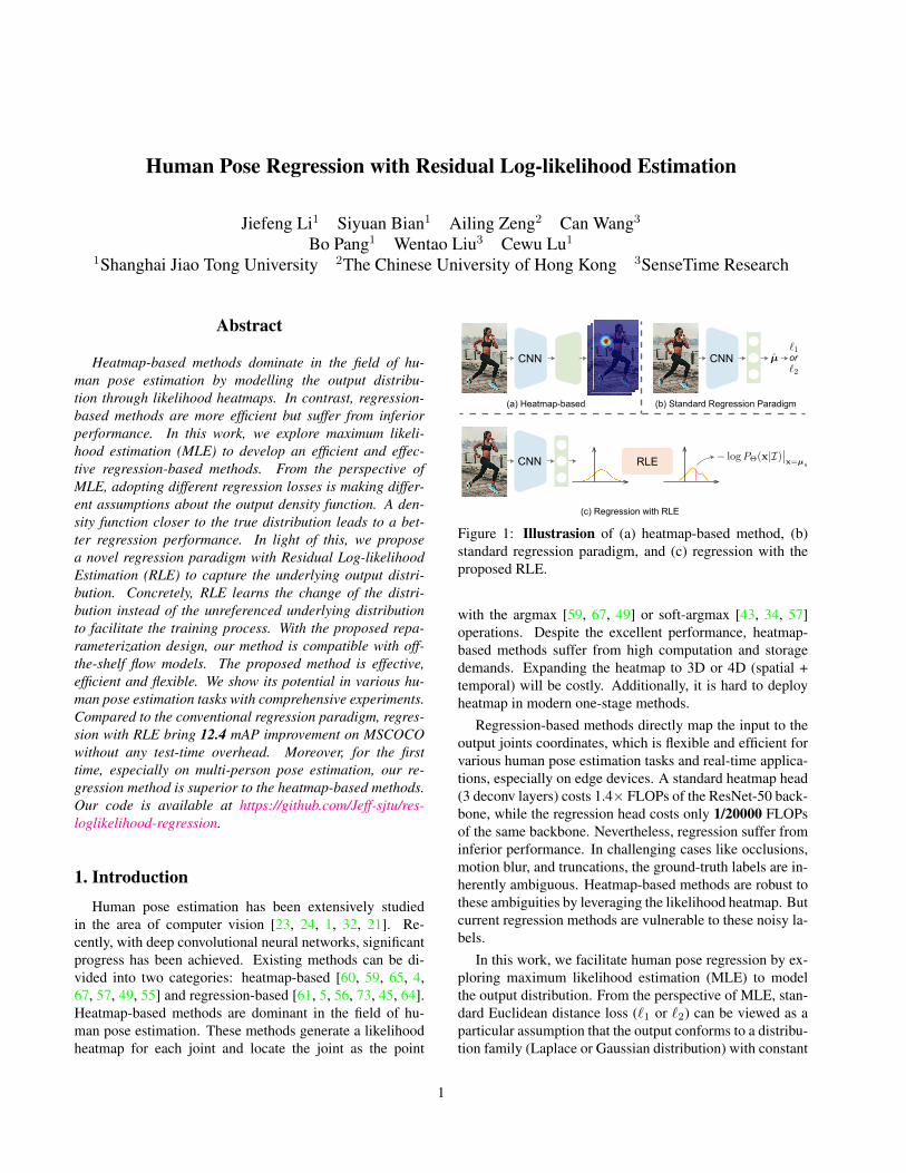
(a) Heatmap-based
(c) Regression with RLE
CNN�1
�2CNN µ or
(b) Standard Regression Paradigm
RLECNN − logPΘ(x|I)∣∣x=µg
Figure 1: Illustrasion of (a) heatmap-based method, (b)standard regression paradigm, and (c) regression with theproposed RLE.
with the argmax [59, 67, 49] or soft-argmax [43, 34, 57]operations. Despite the excellent performance, heatmap-based methods suffer from high computation and storagedemands. Expanding the heatmap to 3D or 4D (spatial +temporal) will be costly. Additionally, it is hard to deployheatmap in modern one-stage methods.
Regression-based methods directly map the input to theoutput joints coordinates, which is flexible and efficient forvarious human pose estimation tasks and real-time applica-tions, especially on edge devices. A standard heatmap head(3 deconv layers) costs 1.4× FLOPs of the ResNet-50 back-bone, while the regression head costs only 1/20000 FLOPsof the same backbone. Nevertheless, regression suffer frominferior performance. In challenging cases like occlusions,motion blur, and truncations, the ground-truth labels are in-herently ambiguous. Heatmap-based methods are robust tothese ambiguities by leveraging the likelihood heatmap. Butcurrent regression methods are vulnerable to these noisy la-bels.
In this work, we facilitate human pose regression by ex-ploring maximum likelihood estimation (MLE) to modelthe output distribution. From the perspective of MLE, stan-dard Euclidean distance loss (`1 or `2) can be viewed as aparticular assumption that the output conforms to a distribu-tion family (Laplace or Gaussian distribution) with constant
1
variance. Intuitively, the regression performance can be im-proved if we construct the likelihood function with the trueunderlying distribution instead of the inappropriate hypoth-esis.
To this end, we propose a novel and effective regres-sion paradigm, named Residual Log-likelihood Estimation(RLE), that leverages normalizing flows to estimate theunderlying distribution and boosts human pose regression.Given a tractable preset assumption of the likelihood func-tion, RLE estimates the residual log-likelihood, i.e. thechange of the distribution. It is easier to be optimized com-pared to the original unreferenced underlying distribution.Besides, we design a reparameterization strategy for theflow model to learn the intrinsic characteristics of the un-derlying distribution. This strategy makes our regressionframework feasible and allows us to utilize the off-the-shelfflow model to approximate the distribution without a so-phisticated network architecture.
During training, the regression model and the RLE mod-ule can be optimized simultaneously. Since the form of theunderlying distribution is unknown, the RLE module is alsotrained via the maximum likelihood estimation process. Be-sides, the RLE module does not participate in the inferencephase. In other words, the proposed method can bring sig-nificant improvement to the regression model without anytest-time overhead.
The proposed regression framework is general. It can beapplied to various human pose estimation algorithms (e.g.two-stage approaches [48, 15, 13, 67, 55], one-stage ap-proaches [73, 45, 64]) and various tasks (e.g. single andmulti-person 2D/3D pose estimation [1, 32, 21, 38, 23, 24]).We benchmark the proposed method on three pose estima-tion datasets, including MPII [1], MSCOCO [32] and Hu-man3.6M [21]. With a simple yet effective architecture,RLE boosts the conventional regression method by 12.4mAP and achieves superior performance to the heatmap-based methods. Moreover, it is more computation and stor-age efficient than heatmap-based methods. Specifically,on the MSCOCO dataset [32], our regression-based modelwith ResNet-50 [16] backbone achieves 71.3 mAP with4.0 GFLOPs, compared to 71.0 mAP with 9.7 GFLOPs ofheatmap-based SimplePose [67]. We hope our method willinspire the field to rethink the potential of regression-basedmethods.
The contributions of our approach can be summarized asfollows:
• We propose a novel and effective regression paradigmwith the reparameterization design and Residual Log-likelihood Estimation (RLE). The proposed methodboosts human pose regression without any test-timeoverhead.
• For the first time, regression-based methods achieve
superior performance to the heatmap-based methods,and it is more computation and storage efficient.
• We show the potential of the proposed paradigm byapplying it to various human pose estimation methods.Considerable improvements are observed in all thesemethods.
2. Related WorkHeatmap-based Pose Estimation. The idea of utilizinglikelihood heatmaps to represent human joint locations isproposed by Tompson et al. [60]. Since then, heatmap-based approaches dominate in the field of 2D human poseestimation. Pioneer works [60, 59, 65, 42] design pow-erful CNN models to estimate heatmaps for single-personpose estimation. Many works [48, 15, 13, 67, 30, 55] ex-tend this idea to multi-person pose estimation following thetop-down framework, i.e. detection and single-person poseestimation. In the bottom-up framework [51, 20, 22, 4, 41,47, 8], multiple body joints are retrieved from the heatmapsand grouped into different human poses. Pavlakos et al. [49]first extend the heatmap to 3D space. The 3D heatmap rep-resentation is followed by several works [57, 39, 7, 72, 62,31]. Sun et al. [57] leverage the soft-argmax operation to re-trieve joint locations from heatmaps in a differentiable man-ner, which allows end-to-end training. It prevents quantiza-tion error, but the model is still required to generate high-resolution features and heatmaps.
Regression-based Pose Estimation. In the context of hu-man pose estimation, only a few works are regression-based. Toshev et al. [61] first leverage the convolutionalnetwork for human pose estimation. Carreira et al. [5] pro-pose an Iterative Error Feedback (IEF) network to improvethe performance of the regression model. Zhou et al. [73]and Tian et al. [58] propose direct pose regression in theone-stage object detection framework. Nie et al. [45] factor-ize the long-range displacement into accumulative shorterones. However, it is vulnerable to occlusions. Wei et al. [64]regress the displacement w.r.t. the pre-defined pose anchors.In 3D pose estimation, Sun et al. [56] propose composi-tional pose regression to learn the internal structures of 3Dhuman pose. Rogez et al. [53, 54] classify the human poseinto a set of K anchor-poses and a regression module is pro-posed to refine the anchor to the final prediction. Two-stagemethods [36, 14, 50, 71, 63, 10, 33, 70] lift the 2D poses to3D space by regression. But the 2D poses are still predictedby the heatmap-based 2D pose estimator. Despite lots ofprogress that have been made by previous works, there isstill a huge performance gap between the pure regression-based approaches and the heatmap-based approaches.
In this work, for the first time, we improve the perfor-mance of the regression-based approach to a comparable
2
level of the heatmap-based approaches. Our method is flex-ible and can be applied to various human pose estimationalgorithms.
Normalizing Flow in Human Pose Estimation. Somerecent works leverage normalizing flows to build priors in3D human pose estimation. Xu et al. [68] propose new 3Dhuman shape and articulated pose models with the kine-matic prior based on normalizing flows. Zanfir et al. [69]use normalizing flows to build a prior on SMPL joint an-gles for their weakly-supervised method. Biggs et al. [3]learn a pose prior by normalizing flows to sample the bestoutput from the ambiguous image. Different from previousmethods, we leverage normalizing flows to estimate the un-derlying output distribution.
Adaptive Loss Function. In our method, the output dis-tribution is learnable, which resulting in a learnable lossfunction. There have been several works towards adaptiveloss functions. Imani et al. [19] propose histogram loss,which use histogram (i.e. heatmap) to represent the outputdistribution. Some works define a superset of loss functionsand change the loss by tuning the parameters of the func-tion. Wu et al. [66] using a teacher model to dynamicallychange the loss function of the student model. Barron [2]presents a generalization of common loss functions, whichautomatically adapts itself during training. Different fromprevious methods, we do not set the form of the distribu-tion family in advance. The loss function can learn to bearbitrary forms within the maximum likelihood estimationframework.
3. MethodIn this work, we aim at improving the performance of
the regression-based method to a competitive level of theheatmap-based method. Compared with the heatmap-basedmethod, regression-based method has lots of merits: i) Itgets rid of the high-resolution heatmaps and has low com-putation and storage complexity. ii) It has a continuousoutput and does not suffer from the quantization problem.iii) It can be extended to a wide variety of scenarios (e.g.one-stage methods, video-based methods, 3D scenes) at aminimal cost. However, existing regression-based methodssuffer from poor performance, which is fatal and restricts itswide usage.
In this section, before introducing our solution, we firstreview the general formulation of regression from the per-spective of maximum likelihood estimation in §3.1. Then,in §3.2, we present the Residual Log-likelihood Estimation(RLE), an approach that leverages normalizing flows to cap-ture the underlying residual log-likelihood function and fa-cilitate human pose regression. Finally, the necessary im-
plementation details are provided in §3.3.
3.1. General Formulation of Regression
The standard regression paradigm is to apply `1 or `2loss to the regressed output µ. Loss functions are empir-ically chosen for different tasks. Here, we review the re-gression problem from the perspective of maximum likeli-hood estimation (MLE). Given an input image I, the regres-sion model predicts a distribution PΘ(x|I) that indicatesthe probability of the ground truth appearing in the locationx, where Θ denotes the learnable model parameters. Dueto the inherent ambiguities in the labels, the labelled loca-tion µg can be viewed as an observation sampled near theground truth by the human annotator. The learning processis to optimize the model parameters Θ that makes the ob-served label µg most probable. Therefore, the loss functionof this maximum likelihood estimation (MLE) process isdefined as:
Lmle = − logPΘ(x|I)∣∣∣x=µg
. (1)
In this formulation, different regression losses are es-sentially different hypotheses of the output probability dis-tribution. For example, in some works of object detec-tion [18, 29, 28] and dense correspondences [40], the den-sity is assumed to be a Gaussian distribution. The modelneeds to predict two values, µ and σ, to construct the den-
sity function PΘ(x|I) = 1√2πσ
e−(x−µ)2
2σ2 . To maximize thelikelihood of the observed label µg , the loss function be-comes:
L = − logPΘ(x|I)∣∣∣x=µg
∝ log σ +(µg − µ)2
2σ2 . (2)
If we assume the density function has a constant variance,i.e. σ is a constant, the loss degenerates to standard `2 loss:L = (µg − µ)2. Further, if we assume the density fol-lows the Laplace distribution with a constant variance, theloss function becomes the standard `1 loss. In the inferencephase, the value µ used to control the location of distribu-tion serves as the regressed output.
From this perspective, the loss function depends on theshape of the distribution PΘ(x|I). Therefore, a more accu-rate density function could lead to better results. However,since the analytical expression of the underlying distribu-tion is unknown, the model can not simply regress severalvalues to construct the density function like Eq. 2. To esti-mate the underlying distribution and facilitate human poseregression, in the following section, we propose a novel re-gression paradigm by leveraging normalizing flow.
3.2. Regression with Normalizing Flows
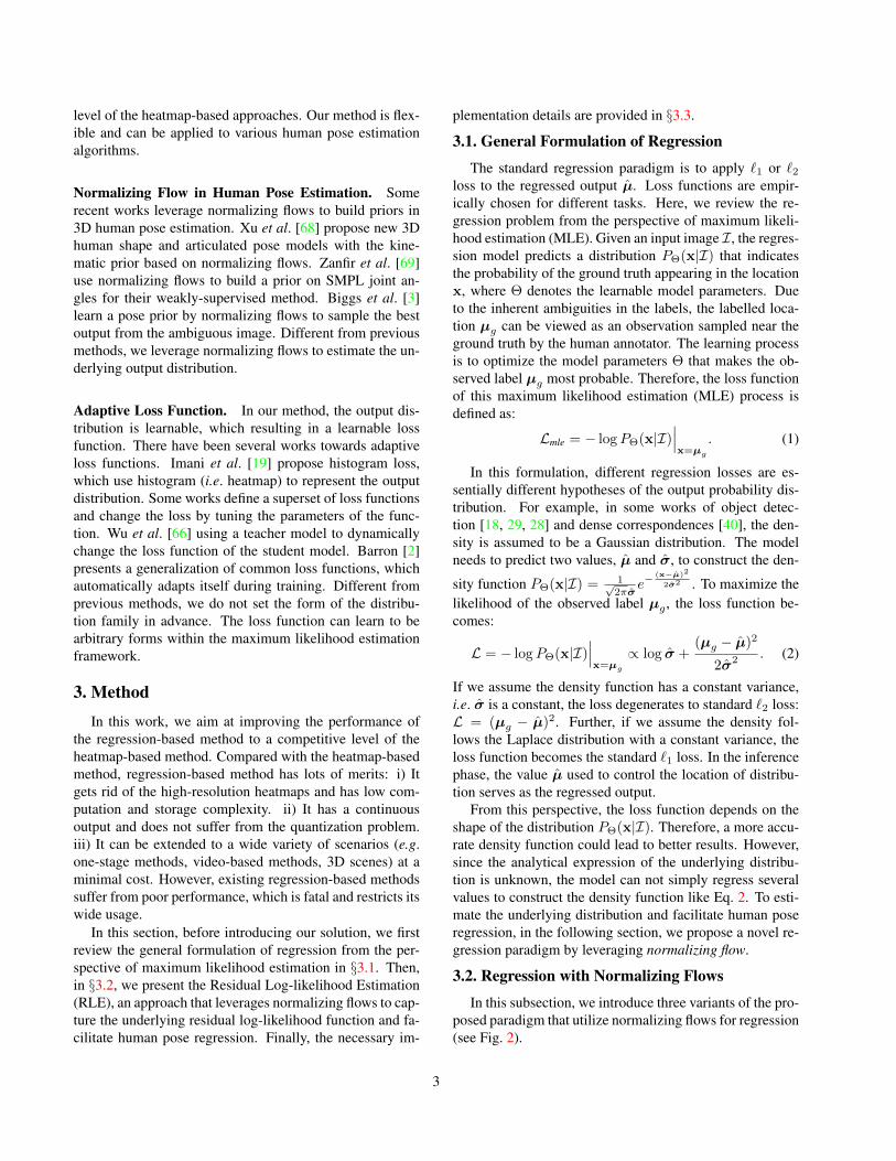
In this subsection, we introduce three variants of the pro-posed paradigm that utilize normalizing flows for regression(see Fig. 2).
3
Basic Design. The basic design of the proposed regres-sion paradigm with normalizing flows is illustrated inFig. 2(a). Here, normalizing flows [52, 11, 26, 46, 25] learnto construct a complex distribution by transforming a sim-ple distribution through an invertible mapping. We considerthe distribution PΘ(z|I) on a random variable z as the ini-tial density function. It is defined by the output µ and σfrom the regression model Θ. For simplicity, we assume
PΘ(z|I) = 1√2πσ
e−(z−µ)2
2σ2 , i.e. the Gaussian distribution.A smooth and invertible mapping fφ : R2 → R2 is chosento transform z to x, i.e. x = fφ(z), where φ is the learnableparameters of the flow model.
The transformed variable x follows another distributionPΘ,φ(x|I). The probability density function PΘ,φ(x|I) de-pends on both the regression model Θ and the flow modelfφ, which can be calculated as:
logPΘ,φ(x|I) = logPΘ(z|I) + log
∣∣∣∣∣det∂f−1
φ
∂x
∣∣∣∣∣ , (3)
where f−1φ is the inverse of fφ and z = f−1
φ (x). In this way,given arbitrary x, the corresponding log-probability can beestimated through Eq. 3 by reversely computing z. Besides,PΘ,φ(x|I) is learnable and can fit arbitrary distribution aslong as fφ is complex enough. In practice, we can composeseveral simple mappings successively to construct arbitrar-ily complex functions, i.e. x = fφ(z) = fK◦· · ·◦f2◦f1(z).
The maximum likelihood process is performed on thelearned distribution PΘ,φ(x|I). Hence, the loss functionis formulated as:
Lmle = − logPΘ,φ(x|I)∣∣∣x=µg
= − logPΘ(f−1φ (µg) | I)− log
∣∣∣∣∣det∂f−1
φ
∂µg
∣∣∣∣∣ .(4)
Note that the underlying optimal distribution Popt(x|I)is unknown. The flow model is learned in an unsupervisedmanner by maximizing the likelihood of the labelled loca-tions. For example, for the challenging cases (e.g. occlu-sions) with larger deviations in the labels from human an-notators, the predicted distribution should have a large vari-ance to maximize the log-probability.
Reparameterization. Although the basic design seemsreasonable, it is not feasible in practice. The learning of fφ
relies on the terms log
∣∣∣∣det∂f−1φ
∂µg
∣∣∣∣ and f−1φ (µg) in the loss
function (Eq. 4). Therefore, φ will learn to fit the distribu-tion of µg across all images. Nevertheless, the distributionthat we want to learn is about how the output deviates fromthe ground truth conditioning on the input image, not thedistribution of the ground truth itself across all images.
µ
σRegression
NormalizingFlow
PΘ,φ(x|I)PΘ(z|I)Image
x = fφ(z)
(a) Basic Design
×Normalizing
Flow
PΘ,φ(x|I)
Q(x)
Pφ(x)
Reparameterization
ResidualLog-likelihood
Gφ(x)
µ
σRegressionImage x = x · σ + µ
x = fφ(z)
(c) Residual log-likelihood estimation with reparameterization
(b) Direct likelihood estimation with reparameterization
µ
σRegression
Reparameterization
NormalizingFlow
PΘ,φ(x|I)
Pφ(x)N (0, I)
Image x = x · σ + µ
x = fφ(z)
Figure 2: Illustrasion of the proposed regression frame-works. (a) The basic design. (b) Direct likelihood esti-mation with reparameterization. (c) Residual log-likelihoodestimation with reparameterization.
Here, to make our regression framework feasible andcompatible with the off-the-shelf flow models, we furtherdesign the regression paradigm with the reparameterizationstrategy. The new paradigm is illustrated in Fig. 2(b). Weassume all the underlying distribution share the same den-sity function family but with different mean and varianceconditioning on the input I. Firstly, the flow model fφis leveraged to map a zero-mean initial distribution z ∼N (0, I) to a zero-mean deformed distribution x ∼ Pφ(x).Then the regression model Θ predicts two values, µ andσ, to control the position and scale of the distribution.The final distribution PΘ,φ(x|I) is obtained by shifting andrescaling x to x, where x = x · σ + µ.
Therefore, the loss function with reparameterization canbe written as:
Lmle = − logPΘ,φ(x|I)∣∣∣x=µg
= − logPφ(µg)− log
∣∣∣∣det∂µg∂µg
∣∣∣∣
= − logPφ(µg) + log σ,
(5)
where µg = (µg − µ)/σ, and ∂µg/∂µg = 1/σ. With thereparameterization design, now the flow model can focus onlearning the distribution of µg , which reflects the deviationof the output from the ground truth.
4
Residual Log-likelihood Estimation. After reparameter-ization, the regression framework can be trained in an end-to-end manner. The training of the regressed value µ andthe flow model fφ are coupled together, depending on theterm logPφ(µg) in the loss function (Eq. 5). However, thereare intricate dependencies between these two models. Thetraining of the regression model entirely relies on the dis-tribution estimated by the flow model fφ. At the beginningstage of training, the shape of the distribution is far fromcorrect, which increases the difficulty to train the regressionmodel and might degrade the model performance.
To facilitate the training process, we develop a gradientshortcut to reduce the dependence between these two mod-els. Formally, the distribution estimated by the flow modelPφ(x) is trying to fit the optimal underlying distributionPopt(x), which can be split into three terms:
logPopt(x) = log
(Q(x) · Popt(x)
s ·Q(x)· s)
= logQ(x) + logPopt(x)
s ·Q(x)+ log s,
(6)
where the termQ(x) can be a simple distribution, e.g. Gaus-sian distribution Q(x) = N (0, I), the term log
Popt(x)s·Q(x) is
what we call residual log-likelihood, and the constant s isto make sure the residual term is a distribution. We assumethatQ(x) can roughly match the underlying distribution butnot perfectly. The residual log-likelihood is to compen-sate for the difference. Thus, we split the log-probabilityof Pφ(x) the same way as Eq. 6:
logPφ(x) = logQ(x) + logGφ(x) + log s, (7)
where Gφ(x) is the distribution learned by the flow model.The value of s = 1∫
Gφ(x)Q(x)dxcan be approximated by
the Riemann sum. The derivation of s is provided in thesupplemental document.
In this way, Gφ(x) will try to fit the underlying resid-ual likelihood Popt(x)
s·Q(x) instead of learning the entire distri-bution. Finally, combining the reparameterization design(Eq. 5) and residual log-likelihood estimation (Eq. 7), thetotal loss function can be defined as:
Lrle = − logPΘ,φ(x|I)∣∣∣x=µg
= − logPφ(µg) + log σ
= − logQ(µg)− logGφ(µg)− log s+ log σ.
(8)
This process is illustrated in Fig. 2(c).During training, the backward propagated gradients from
Q(µg) do not depend on the flow model, which acceleratesthe training of the regression model. Besides, as the hypoth-esis of ResNet [16], it is easier to optimize the residual map-ping than to optimize the original unreferenced mapping.
To the extreme, if the preset approximation Q(x) is opti-mal, it would be easier to push the residual log-probabilityto zero than to fit an identity mapping by a stack of invert-ible mappings in fφ. The effectiveness of the residual log-likelihood estimation is validated in §4.1.
3.3. Implementation Details
In the training phase, the regression model and the flowmodel are simultaneously optimized in an end-to-end man-ner. We replace the standard regression loss (`1 and `2)with the proposed residual log-likelihood estimation lossLrle. The initial density is set to Laplace distribution bydefault. In the testing phase, the predicted mean µ servesas the regressed output. Therefore, the flow model does notneed to be run during inference. This characteristic makesthe proposed method flexible and easy to apply to variousregression algorithms without any test-time overhead. Be-sides, the prediction confidence can be obtained from σ:
c = 1− 1
K
K∑
i
σi, (9)
where σi is the learned deviation of the ith joint, and Kdenotes the total number of joints. The deviation σi is pre-dicted with a sigmoid function. Hence we have σi ∈ (0, 1)and c ∈ (0, 1).
Flow Model. The proposed regression paradigm is agnos-tic to the flow models. Hence, various off-the-shelf flowmodels [52, 11, 26, 46, 25] can be applied. In the experi-ments, we adopt RealNVP [11] for fast training. We denotethe invertible function with Lfc fully-connected layers withNn neurons as Lfc × Nn. We set Lfc = 3 and Nn = 64by default. The flow model is light-weighted and barely af-fects the training speed. More detailed descriptions of theflow model architecture are provided in the supplementaldocument (§A).
Tasks. The proposed regression paradigm is general andis ready for various human pose estimation tasks. In the ex-periments, we validate the proposed regression paradigm onseven different algorithms in five tasks: single-person 2Dpose estimation, top-down 2D pose estimation, one-stage2D pose estimation, single-stage 3D pose estimation andtwo-stage 3D pose estimation. Detailed training settings areprovided in §4 and §5. The experiments on single-person2D pose estimation are provided in the supplemental docu-ment.
4. Experiments on COCOWe first evaluate the proposed regression paradigm on a
large-scale in-the-wild 2D human pose benchmark COCOKeypoint [32].
5
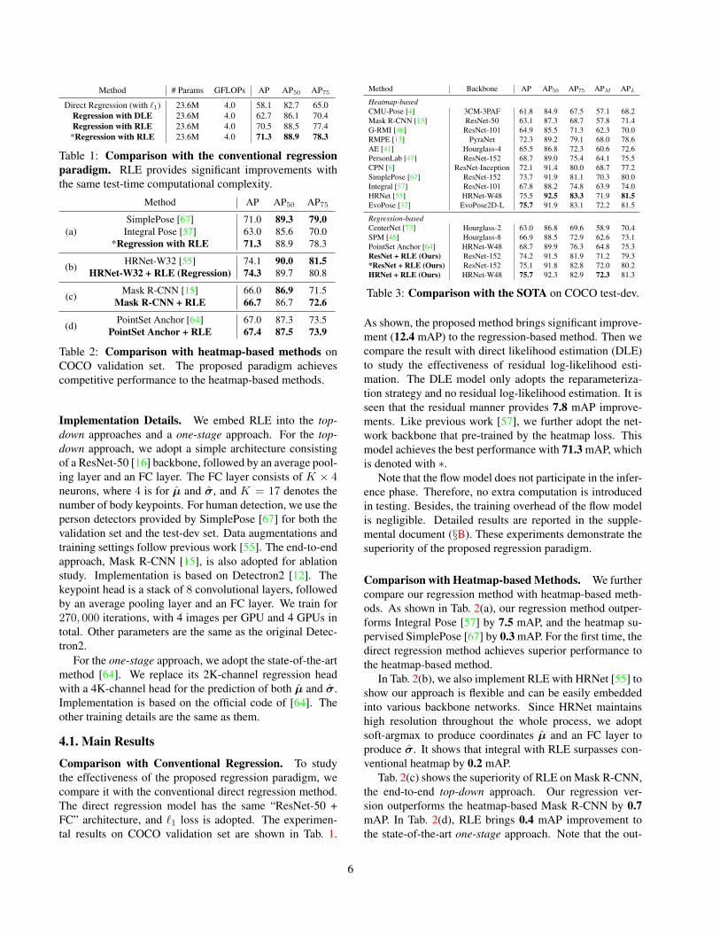
Method # Params GFLOPs AP AP50 AP75
Direct Regression (with `1) 23.6M 4.0 58.1 82.7 65.0Regression with DLE 23.6M 4.0 62.7 86.1 70.4Regression with RLE 23.6M 4.0 70.5 88.5 77.4*Regression with RLE 23.6M 4.0 71.3 88.9 78.3
Table 1: Comparison with the conventional regressionparadigm. RLE provides significant improvements withthe same test-time computational complexity.
Method AP AP50 AP75
(a)SimplePose [67] 71.0 89.3 79.0
Integral Pose [57] 63.0 85.6 70.0*Regression with RLE 71.3 88.9 78.3
(b) HRNet-W32 [55] 74.1 90.0 81.5HRNet-W32 + RLE (Regression) 74.3 89.7 80.8
(c) Mask R-CNN [15] 66.0 86.9 71.5Mask R-CNN + RLE 66.7 86.7 72.6
(d) PointSet Anchor [64] 67.0 87.3 73.5PointSet Anchor + RLE 67.4 87.5 73.9
Table 2: Comparison with heatmap-based methods onCOCO validation set. The proposed paradigm achievescompetitive performance to the heatmap-based methods.
Implementation Details. We embed RLE into the top-down approaches and a one-stage approach. For the top-down approach, we adopt a simple architecture consistingof a ResNet-50 [16] backbone, followed by an average pool-ing layer and an FC layer. The FC layer consists of K × 4neurons, where 4 is for µ and σ, and K = 17 denotes thenumber of body keypoints. For human detection, we use theperson detectors provided by SimplePose [67] for both thevalidation set and the test-dev set. Data augmentations andtraining settings follow previous work [55]. The end-to-endapproach, Mask R-CNN [15], is also adopted for ablationstudy. Implementation is based on Detectron2 [12]. Thekeypoint head is a stack of 8 convolutional layers, followedby an average pooling layer and an FC layer. We train for270, 000 iterations, with 4 images per GPU and 4 GPUs intotal. Other parameters are the same as the original Detec-tron2.
For the one-stage approach, we adopt the state-of-the-artmethod [64]. We replace its 2K-channel regression headwith a 4K-channel head for the prediction of both µ and σ.Implementation is based on the official code of [64]. Theother training details are the same as them.
4.1. Main Results
Comparison with Conventional Regression. To studythe effectiveness of the proposed regression paradigm, wecompare it with the conventional direct regression method.The direct regression model has the same “ResNet-50 +FC” architecture, and `1 loss is adopted. The experimen-tal results on COCO validation set are shown in Tab. 1.
Method Backbone AP AP50 AP75 APM APL
Heatmap-basedCMU-Pose [4] 3CM-3PAF 61.8 84.9 67.5 57.1 68.2Mask R-CNN [15] ResNet-50 63.1 87.3 68.7 57.8 71.4G-RMI [48] ResNet-101 64.9 85.5 71.3 62.3 70.0RMPE [13] PyraNet 72.3 89.2 79.1 68.0 78.6AE [41] Hourglass-4 65.5 86.8 72.3 60.6 72.6PersonLab [47] ResNet-152 68.7 89.0 75.4 64.1 75.5CPN [6] ResNet-Inception 72.1 91.4 80.0 68.7 77.2SimplePose [67] ResNet-152 73.7 91.9 81.1 70.3 80.0Integral [57] ResNet-101 67.8 88.2 74.8 63.9 74.0HRNet [55] HRNet-W48 75.5 92.5 83.3 71.9 81.5EvoPose [37] EvoPose2D-L 75.7 91.9 83.1 72.2 81.5
Regression-basedCenterNet [73] Hourglass-2 63.0 86.8 69.6 58.9 70.4SPM [45] Hourglass-8 66.9 88.5 72.9 62.6 73.1PointSet Anchor [64] HRNet-W48 68.7 89.9 76.3 64.8 75.3ResNet + RLE (Ours) ResNet-152 74.2 91.5 81.9 71.2 79.3*ResNet + RLE (Ours) ResNet-152 75.1 91.8 82.8 72.0 80.2HRNet + RLE (Ours) HRNet-W48 75.7 92.3 82.9 72.3 81.3
Table 3: Comparison with the SOTA on COCO test-dev.
As shown, the proposed method brings significant improve-ment (12.4 mAP) to the regression-based method. Then wecompare the result with direct likelihood estimation (DLE)to study the effectiveness of residual log-likelihood esti-mation. The DLE model only adopts the reparameteriza-tion strategy and no residual log-likelihood estimation. It isseen that the residual manner provides 7.8 mAP improve-ments. Like previous work [57], we further adopt the net-work backbone that pre-trained by the heatmap loss. Thismodel achieves the best performance with 71.3 mAP, whichis denoted with ∗.
Note that the flow model does not participate in the infer-ence phase. Therefore, no extra computation is introducedin testing. Besides, the training overhead of the flow modelis negligible. Detailed results are reported in the supple-mental document (§B). These experiments demonstrate thesuperiority of the proposed regression paradigm.
Comparison with Heatmap-based Methods. We furthercompare our regression method with heatmap-based meth-ods. As shown in Tab. 2(a), our regression method outper-forms Integral Pose [57] by 7.5 mAP, and the heatmap su-pervised SimplePose [67] by 0.3 mAP. For the first time, thedirect regression method achieves superior performance tothe heatmap-based method.
In Tab. 2(b), we also implement RLE with HRNet [55] toshow our approach is flexible and can be easily embeddedinto various backbone networks. Since HRNet maintainshigh resolution throughout the whole process, we adoptsoft-argmax to produce coordinates µ and an FC layer toproduce σ. It shows that integral with RLE surpasses con-ventional heatmap by 0.2 mAP.
Tab. 2(c) shows the superiority of RLE on Mask R-CNN,the end-to-end top-down approach. Our regression ver-sion outperforms the heatmap-based Mask R-CNN by 0.7mAP. In Tab. 2(d), RLE brings 0.4 mAP improvement tothe state-of-the-art one-stage approach. Note that the out-
6
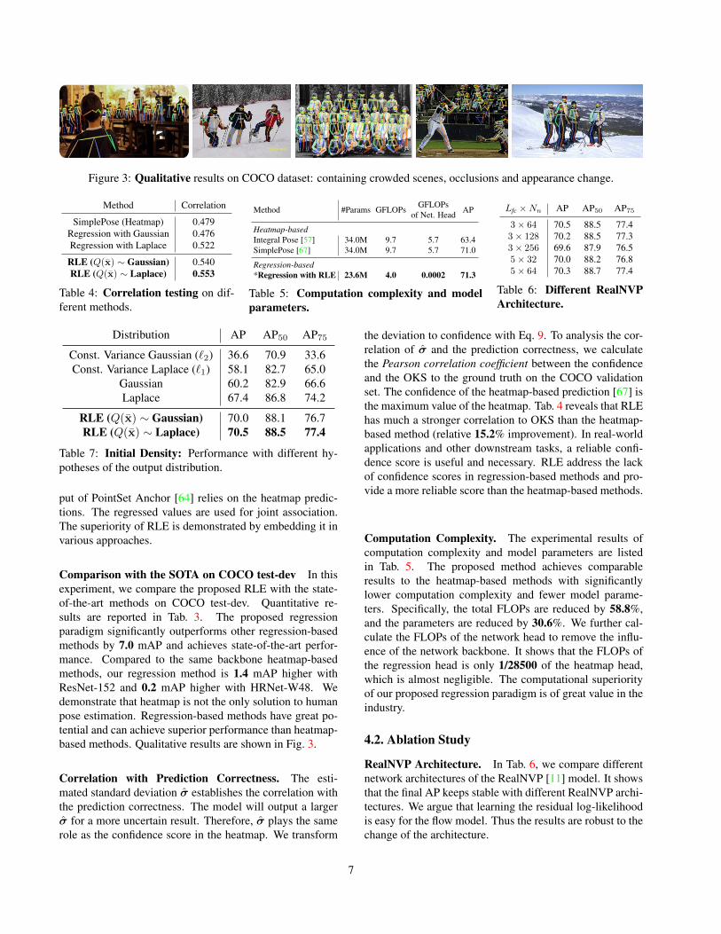
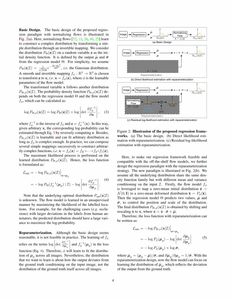
Figure 3: Qualitative results on COCO dataset: containing crowded scenes, occlusions and appearance change.
Method Correlation
SimplePose (Heatmap) 0.479Regression with Gaussian 0.476Regression with Laplace 0.522
RLE (Q(x) ∼ Gaussian) 0.540RLE (Q(x) ∼ Laplace) 0.553
Table 4: Correlation testing on dif-ferent methods.
Method #Params GFLOPsGFLOPs
of Net. Head AP
Heatmap-basedIntegral Pose [57] 34.0M 9.7 5.7 63.4SimplePose [67] 34.0M 9.7 5.7 71.0
Regression-based*Regression with RLE 23.6M 4.0 0.0002 71.3
Table 5: Computation complexity and modelparameters.
Lfc ×Nn AP AP50 AP75
3× 64 70.5 88.5 77.43× 128 70.2 88.5 77.33× 256 69.6 87.9 76.55× 32 70.0 88.2 76.85× 64 70.3 88.7 77.4
Table 6: Different RealNVPArchitecture.
Distribution AP AP50 AP75
Const. Variance Gaussian (`2) 36.6 70.9 33.6Const. Variance Laplace (`1) 58.1 82.7 65.0
Gaussian 60.2 82.9 66.6Laplace 67.4 86.8 74.2
RLE (Q(x) ∼ Gaussian) 70.0 88.1 76.7RLE (Q(x) ∼ Laplace) 70.5 88.5 77.4
Table 7: Initial Density: Performance with different hy-potheses of the output distribution.
put of PointSet Anchor [64] relies on the heatmap predic-tions. The regressed values are used for joint association.The superiority of RLE is demonstrated by embedding it invarious approaches.
Comparison with the SOTA on COCO test-dev In thisexperiment, we compare the proposed RLE with the state-of-the-art methods on COCO test-dev. Quantitative re-sults are reported in Tab. 3. The proposed regressionparadigm significantly outperforms other regression-basedmethods by 7.0 mAP and achieves state-of-the-art perfor-mance. Compared to the same backbone heatmap-basedmethods, our regression method is 1.4 mAP higher withResNet-152 and 0.2 mAP higher with HRNet-W48. Wedemonstrate that heatmap is not the only solution to humanpose estimation. Regression-based methods have great po-tential and can achieve superior performance than heatmap-based methods. Qualitative results are shown in Fig. 3.
Correlation with Prediction Correctness. The esti-mated standard deviation σ establishes the correlation withthe prediction correctness. The model will output a largerσ for a more uncertain result. Therefore, σ plays the samerole as the confidence score in the heatmap. We transform
the deviation to confidence with Eq. 9. To analysis the cor-relation of σ and the prediction correctness, we calculatethe Pearson correlation coefficient between the confidenceand the OKS to the ground truth on the COCO validationset. The confidence of the heatmap-based prediction [67] isthe maximum value of the heatmap. Tab. 4 reveals that RLEhas much a stronger correlation to OKS than the heatmap-based method (relative 15.2% improvement). In real-worldapplications and other downstream tasks, a reliable confi-dence score is useful and necessary. RLE address the lackof confidence scores in regression-based methods and pro-vide a more reliable score than the heatmap-based methods.
Computation Complexity. The experimental results ofcomputation complexity and model parameters are listedin Tab. 5. The proposed method achieves comparableresults to the heatmap-based methods with significantlylower computation complexity and fewer model parame-ters. Specifically, the total FLOPs are reduced by 58.8%,and the parameters are reduced by 30.6%. We further cal-culate the FLOPs of the network head to remove the influ-ence of the network backbone. It shows that the FLOPs ofthe regression head is only 1/28500 of the heatmap head,which is almost negligible. The computational superiorityof our proposed regression paradigm is of great value in theindustry.
4.2. Ablation Study
RealNVP Architecture. In Tab. 6, we compare differentnetwork architectures of the RealNVP [11] model. It showsthat the final AP keeps stable with different RealNVP archi-tectures. We argue that learning the residual log-likelihoodis easy for the flow model. Thus the results are robust to thechange of the architecture.
7
Initial Density. To examine how the assumption of theoutput distribution affects the regression performance in thecontext of MLE, we compare the results of different den-sity functions with our method. The Laplace distributionand Gaussian distribution will degenerate to standard `1 and`2 loss if they are assumed to have constant variances. Asshown in Tab. 7, the learned distributions of our methodprovide more than 21.3% improvements. Besides, we studythe baselines that assuming the output follows the Gaus-sian and Laplace distributions with the learnable deviationσ. The distributions with learnable σ outperform those withconstant variance, but are still inferior to RLE.
Moreover, different initial densities Q(x) for RLE arealso tested. There is a large gap between the original Gaus-sian and Laplace distribution. However, with RLE to learnthe change of the density, the difference between these twodistributions is significantly reduced. It demonstrates thatRLE is robust to different assumptions of the initial density.
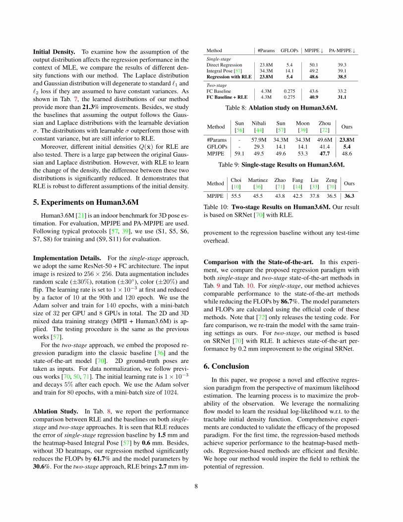
5. Experiments on Human3.6MHuman3.6M [21] is an indoor benchmark for 3D pose es-
timation. For evaluation, MPJPE and PA-MPJPE are used.Following typical protocols [57, 39], we use (S1, S5, S6,S7, S8) for training and (S9, S11) for evaluation.
Implementation Details. For the single-stage approach,we adopt the same ResNet-50 + FC architecture. The inputimage is resized to 256× 256. Data augmentation includesrandom scale (±30%), rotation (±30◦), color (±20%) andflip. The learning rate is set to 1× 10⁻³ at first and reducedby a factor of 10 at the 90th and 120 epoch. We use theAdam solver and train for 140 epochs, with a mini-batchsize of 32 per GPU and 8 GPUs in total. The 2D and 3Dmixed data training strategy (MPII + Human3.6M) is ap-plied. The testing procedure is the same as the previousworks [57].
For the two-stage approach, we embed the proposed re-gression paradigm into the classic baseline [36] and thestate-of-the-art model [70]. 2D ground-truth poses aretaken as inputs. For data normalization, we follow previ-ous works [70, 50, 71]. The initial learning rate is 1× 10⁻³
and decays 5% after each epoch. We use the Adam solverand train for 80 epochs, with a mini-batch size of 1024.
Ablation Study. In Tab. 8, we report the performancecomparison between RLE and the baselines on both single-stage and two-stage approaches. It is seen that RLE reducesthe error of single-stage regression baseline by 1.5 mm andthe heatmap-based Integral Pose [57] by 0.6 mm. Besides,without 3D heatmaps, our regression method significantlyreduces the FLOPs by 61.7% and the model parameters by30.6%. For the two-stage approach, RLE brings 2.7 mm im-
Method #Params GFLOPs MPJPE ↓ PA-MPJPE ↓Single-stageDirect Regression 23.8M 5.4 50.1 39.3Integral Pose [57] 34.3M 14.1 49.2 39.1Regression with RLE 23.8M 5.4 48.6 38.5
Two-stageFC Baseline 4.3M 0.275 43.6 33.2FC Baseline + RLE 4.3M 0.275 40.9 31.1
Table 8: Ablation study on Human3.6M.
MethodSun[56]
Nibali[44]
Sun[57]
Moon[39]
Zhou[72] Ours
#Params - 57.9M 34.3M 34.3M 49.6M 23.8MGFLOPs - 29.3 14.1 14.1 41.4 5.4MPJPE 59.1 49.5 49.6 53.3 47.7 48.6
Table 9: Single-stage Results on Human3.6M.
MethodChoi[10]
Martinez[36]
Zhao[71]
Fang[14]
Liu[33]
Zeng[70] Ours
MPJPE 55.5 45.5 43.8 42.5 37.8 36.5 36.3
Table 10: Two-stage Results on Human3.6M. Our resultis based on SRNet [70] with RLE.
provement to the regression baseline without any test-timeoverhead.
Comparison with the State-of-the-art. In this experi-ment, we compare the proposed regression paradigm withboth single-stage and two-stage state-of-the-art methods inTab. 9 and Tab. 10. For single-stage, our method achievescomparable performance to the state-of-the-art methodswhile reducing the FLOPs by 86.7%. The model parametersand FLOPs are calculated using the official code of thesemethods. Note that [72] only releases the testing code. Forfare comparison, we re-train the model with the same train-ing settings as ours. For two-stage, our method is basedon SRNet [70] with RLE. It achieves state-of-the-art per-formance by 0.2 mm improvement to the original SRNet.
6. Conclusion
In this paper, we propose a novel and effective regres-sion paradigm from the perspective of maximum likelihoodestimation. The learning process is to maximize the prob-ability of the observation. We leverage the normalizingflow model to learn the residual log-likelihood w.r.t. to thetractable initial density function. Comprehensive experi-ments are conducted to validate the efficacy of the proposedparadigm. For the first time, the regression-based methodsachieve superior performance to the heatmap-based meth-ods. Regression-based methods are efficient and flexible.We hope our method would inspire the field to rethink thepotential of regression.
8
References[1] Mykhaylo Andriluka, Leonid Pishchulin, Peter Gehler, and
Bernt Schiele. 2d human pose estimation: New benchmarkand state of the art analysis. In CVPR, 2014. 1, 2, 11, 12
[2] Jonathan T Barron. A general and adaptive robust loss func-tion. In CVPR, 2019. 3
[3] Benjamin Biggs, Sebastien Ehrhadt, Hanbyul Joo, BenjaminGraham, Andrea Vedaldi, and David Novotny. 3d multi-bodies: Fitting sets of plausible 3d human models to am-biguous image data. In NeurIPS, 2020. 3
[4] Zhe Cao, Tomas Simon, Shih-En Wei, and Yaser Sheikh.Realtime multi-person 2d pose estimation using part affinityfields. In CVPR, 2017. 1, 2, 6
[5] Joao Carreira, Pulkit Agrawal, Katerina Fragkiadaki, and Ji-tendra Malik. Human pose estimation with iterative errorfeedback. In CVPR, 2016. 1, 2
[6] Yilun Chen, Zhicheng Wang, Yuxiang Peng, ZhiqiangZhang, Gang Yu, and Jian Sun. Cascaded pyramid networkfor multi-person pose estimation. In CVPR, 2018. 6
[7] Zerui Chen, Yiru Guo, Yan Huang, and Liang Wang. Learn-ing depth-aware heatmaps for 3d human pose estimation inthe wild. In BMVC, 2019. 2
[8] Bowen Cheng, Bin Xiao, Jingdong Wang, Honghui Shi,Thomas S Huang, and Lei Zhang. Higherhrnet: Scale-awarerepresentation learning for bottom-up human pose estima-tion. In CVPR, 2020. 2
[9] Stephanie J Chiu, Michael J Allingham, Priyatham S Mettu,Scott W Cousins, Joseph A Izatt, and Sina Farsiu. Kernel re-gression based segmentation of optical coherence tomogra-phy images with diabetic macular edema. Biomedical opticsexpress, 2015. 14
[10] Hongsuk Choi, Gyeongsik Moon, and Kyoung Mu Lee.Pose2mesh: Graph convolutional network for 3d human poseand mesh recovery from a 2d human pose, 2020. 2, 8
[11] Laurent Dinh, Jascha Sohl-Dickstein, and Samy Bengio.Density estimation using real nvp. In ICRL, 2016. 4, 5, 7, 11
[12] facebookresearch. Detectron2. https://github.com/facebookresearch/detectron2, 2021. 6
[13] Hao-Shu Fang, Shuqin Xie, Yu-Wing Tai, and Cewu Lu.Rmpe: Regional multi-person pose estimation. In ICCV,2017. 2, 6
[14] Hao-Shu Fang, Yuanlu Xu, Wenguan Wang, Xiaobai Liu,and Song-Chun Zhu. Learning pose grammar to encode hu-man body configuration for 3d pose estimation. In AAAI,2018. 2, 8
[15] Kaiming He, Georgia Gkioxari, Piotr Dollar, and Ross Gir-shick. Mask r-cnn. In ICCV, 2017. 2, 6
[16] Kaiming He, Xiangyu Zhang, Shaoqing Ren, and Jian Sun.Deep residual learning for image recognition. In CVPR,2016. 2, 5, 6
[17] Yufan He, Aaron Carass, Yihao Liu, Bruno M Jedynak,Sharon D Solomon, Shiv Saidha, Peter A Calabresi, andJerry L Prince. Fully convolutional boundary regression forretina oct segmentation. In MICCAI, 2019. 14
[18] Yihui He, Chenchen Zhu, Jianren Wang, Marios Savvides,and Xiangyu Zhang. Bounding box regression with uncer-tainty for accurate object detection. In CVPR, 2019. 3
[19] Ehsan Imani and Martha White. Improving regression per-formance with distributional losses. In ICML, 2018. 3
[20] Eldar Insafutdinov, Leonid Pishchulin, Bjoern Andres,Mykhaylo Andriluka, and Bernt Schiele. Deepercut: Adeeper, stronger, and faster multi-person pose estimationmodel. In ECCV, 2016. 2
[21] Catalin Ionescu, Dragos Papava, Vlad Olaru, and CristianSminchisescu. Human3.6m: Large scale datasets and predic-tive methods for 3D human sensing in natural environments.TPAMI, 2014. 1, 2, 8, 12
[22] Umar Iqbal and Juergen Gall. Multi-person pose estimationwith local joint-to-person associations. In ECCV, 2016. 2
[23] Sam Johnson and Mark Everingham. Clustered pose andnonlinear appearance models for human pose estimation. InBMVC, 2010. 1, 2
[24] Sam Johnson and Mark Everingham. Learning effective hu-man pose estimation from inaccurate annotation. In CVPR,2011. 1, 2
[25] Diederik P Kingma and Prafulla Dhariwal. Glow: Genera-tive flow with invertible 1x1 convolutions. In NeurIPS, 2018.4, 5
[26] Diederik P Kingma, Tim Salimans, Rafal Jozefowicz, XiChen, Ilya Sutskever, and Max Welling. Improving varia-tional inference with inverse autoregressive flow, 2016. 4,5
[27] Muhammed Kocabas, Chun-Hao P Huang, Otmar Hilliges,and Michael J Black. Pare: Part attention regressor for 3dhuman body estimation. arXiv preprint arXiv:2104.08527,2021. 12
[28] Youngwan Lee, Joong-won Hwang, Hyung-Il Kim, KiminYun, and Joungyoul Park. Localization uncertainty esti-mation for anchor-free object detection. arXiv preprintarXiv:2006.15607, 2020. 3
[29] Chen Li and Gim Hee Lee. Generating multiple hypothesesfor 3d human pose estimation with mixture density network.In CVPR, 2019. 3
[30] Jiefeng Li, Can Wang, Hao Zhu, Yihuan Mao, Hao-ShuFang, and Cewu Lu. Crowdpose: Efficient crowded scenespose estimation and a new benchmark. In CVPR, 2019. 2
[31] Jiefeng Li, Chao Xu, Zhicun Chen, Siyuan Bian, Lixin Yang,and Cewu Lu. Hybrik: A hybrid analytical-neural inversekinematics solution for 3d human pose and shape estimation.In CVPR, 2021. 2
[32] Tsung-Yi Lin, Michael Maire, Serge Belongie, James Hays,Pietro Perona, Deva Ramanan, Piotr Dollar, and C LawrenceZitnick. Microsoft COCO: Common objects in context. InECCV, 2014. 1, 2, 5, 12
[33] Kenkun Liu, Rongqi Ding, Zhiming Zou, Le Wang, and WeiTang. A comprehensive study of weight sharing in graphnetworks for 3d human pose estimation, 2020. 2, 8
[34] Diogo C Luvizon, Hedi Tabia, and David Picard. Humanpose regression by combining indirect part detection andcontextual information. Computers & Graphics, 2019. 1
[35] Andrew L Maas, Awni Y Hannun, and Andrew Y Ng. Recti-fier nonlinearities improve neural network acoustic models.In ICML, 2013. 11
9
[36] Julieta Martinez, Rayat Hossain, Javier Romero, and James JLittle. A simple yet effective baseline for 3d human poseestimation. In ICCV, 2017. 2, 8
[37] William McNally, Kanav Vats, Alexander Wong, and JohnMcPhee. Evopose2d: Pushing the boundaries of 2d hu-man pose estimation using neuroevolution. arXiv preprintarXiv:2011.08446, 2020. 6
[38] Dushyant Mehta, Helge Rhodin, Dan Casas, PascalFua, Oleksandr Sotnychenko, Weipeng Xu, and ChristianTheobalt. Monocular 3D human pose estimation in the wildusing improved cnn supervision, 2017. 2
[39] Gyeongsik Moon, Ju Yong Chang, and Kyoung Mu Lee.Camera distance-aware top-down approach for 3D multi-person pose estimation from a single rgb image. In ICCV,2019. 2, 8
[40] Natalia Neverova, David Novotny, and Andrea Vedaldi. Cor-related uncertainty for learning dense correspondences fromnoisy labels. In NeurIPS, 2019. 3
[41] Alejandro Newell, Zhiao Huang, and Jia Deng. Associa-tive embedding: End-to-end learning for joint detection andgrouping. In NeurIPS, 2017. 2, 6
[42] Alejandro Newell, Kaiyu Yang, and Jia Deng. Stacked hour-glass networks for human pose estimation. In ECCV, 2016.2
[43] Aiden Nibali, Zhen He, Stuart Morgan, and Luke Prender-gast. Numerical coordinate regression with convolutionalneural networks. arXiv preprint arXiv:1801.07372, 2018. 1
[44] Aiden Nibali, Zhen He, Stuart Morgan, and Luke Prender-gast. 3d human pose estimation with 2d marginal heatmaps.In WACV, 2019. 8
[45] Xuecheng Nie, Jiashi Feng, Jianfeng Zhang, and ShuichengYan. Single-stage multi-person pose machines. In ICCV,2019. 1, 2, 6
[46] George Papamakarios, Theo Pavlakou, and Iain Murray.Masked autoregressive flow for density estimation, 2017. 4,5
[47] George Papandreou, Tyler Zhu, Liang-Chieh Chen, SpyrosGidaris, Jonathan Tompson, and Kevin Murphy. Person-lab: Person pose estimation and instance segmentation witha bottom-up, part-based, geometric embedding model. InECCV, 2018. 2, 6
[48] George Papandreou, Tyler Zhu, Nori Kanazawa, AlexanderToshev, Jonathan Tompson, Chris Bregler, and Kevin Mur-phy. Towards accurate multi-person pose estimation in thewild. In CVPR, 2017. 2, 6
[49] Georgios Pavlakos, Xiaowei Zhou, Konstantinos G Derpa-nis, and Kostas Daniilidis. Coarse-to-fine volumetric predic-tion for single-image 3d human pose, 2017. 1, 2
[50] Dario Pavllo, Christoph Feichtenhofer, David Grangier, andMichael Auli. 3d human pose estimation in video with tem-poral convolutions and semi-supervised training. In CVPR,2019. 2, 8
[51] Leonid Pishchulin, Eldar Insafutdinov, Siyu Tang, BjoernAndres, Mykhaylo Andriluka, Peter V Gehler, and BerntSchiele. Deepcut: Joint subset partition and labeling formulti person pose estimation. In CVPR, 2016. 2
[52] Danilo Rezende and Shakir Mohamed. Variational inferencewith normalizing flows. In ICML, 2015. 4, 5
[53] Gregory Rogez, Philippe Weinzaepfel, and Cordelia Schmid.Lcr-net: Localization-classification-regression for humanpose. In CVPR, 2017. 2
[54] Gregory Rogez, Philippe Weinzaepfel, and Cordelia Schmid.Lcr-net++: Multi-person 2d and 3d pose detection in naturalimages. TPAMI, 2019. 2
[55] Ke Sun, Bin Xiao, Dong Liu, and Jingdong Wang. Deephigh-resolution representation learning for human pose esti-mation. In CVPR, 2019. 1, 2, 6
[56] Xiao Sun, Jiaxiang Shang, Shuang Liang, and Yichen Wei.Compositional human pose regression. In ICCV, 2017. 1, 2,8
[57] Xiao Sun, Bin Xiao, Fangyin Wei, Shuang Liang, and YichenWei. Integral human pose regression. In ECCV, 2018. 1, 2,6, 7, 8, 11, 12
[58] Zhi Tian, Hao Chen, and Chunhua Shen. Directpose: Di-rect end-to-end multi-person pose estimation. arXiv preprintarXiv:1911.07451, 2019. 2
[59] Jonathan Tompson, Ross Goroshin, Arjun Jain, Yann LeCun,and Christoph Bregler. Efficient object localization usingconvolutional networks. In CVPR, 2015. 1, 2
[60] Jonathan J Tompson, Arjun Jain, Yann LeCun, and ChristophBregler. Joint training of a convolutional network and agraphical model for human pose estimation. NeurIPS, 2014.1, 2
[61] Alexander Toshev and Christian Szegedy. Deeppose: Humanpose estimation via deep neural networks. In CVPR, 2014.1, 2
[62] Can Wang, Jiefeng Li, Wentao Liu, Chen Qian, and CewuLu. Hmor: Hierarchical multi-person ordinal relations formonocular multi-person 3d pose estimation. In ECCV, 2020.2
[63] Luyang Wang, Yan Chen, Zhenhua Guo, Keyuan Qian,Mude Lin, Hongsheng Li, and Jimmy S Ren. Generalizingmonocular 3d human pose estimation in the wild, 2019. 2
[64] Fangyun Wei, Xiao Sun, Hongyang Li, Jingdong Wang, andStephen Lin. Point-set anchors for object detection, instancesegmentation and pose estimation. In ECCV, 2020. 1, 2, 6, 7
[65] Shih-En Wei, Varun Ramakrishna, Takeo Kanade, and YaserSheikh. Convolutional pose machines. In CVPR, 2016. 1, 2
[66] Lijun Wu, Fei Tian, Yingce Xia, Yang Fan, Tao Qin, Jian-huang Lai, and Tie-Yan Liu. Learning to teach with dynamicloss functions. In NeurIPS, 2018. 3
[67] Bin Xiao, Haiping Wu, and Yichen Wei. Simple baselinesfor human pose estimation and tracking. In ECCV, 2018. 1,2, 6, 7, 12
[68] Hongyi Xu, Eduard Gabriel Bazavan, Andrei Zanfir,William T Freeman, Rahul Sukthankar, and Cristian Smin-chisescu. Ghum & ghuml: Generative 3d human shape andarticulated pose models. In CVPR, 2020. 3
[69] Andrei Zanfir, Eduard Gabriel Bazavan, Hongyi Xu, BillFreeman, Rahul Sukthankar, and Cristian Sminchisescu.Weakly supervised 3d human pose and shape reconstructionwith normalizing flows. ECCV, 2020. 3
[70] Ailing Zeng, Xiao Sun, Fuyang Huang, Minhao Liu, QiangXu, and Stephen Lin. Srnet: Improving generalization in 3dhuman pose estimation with a split-and-recombine approach.In ECCV, 2020. 2, 8
10
[71] Long Zhao, Xi Peng, Yu Tian, Mubbasir Kapadia, and Dim-itris N. Metaxas. Semantic graph convolutional networks for3d human pose regression. In CVPR, 2019. 2, 8
[72] Kun Zhou, Xiaoguang Han, Nianjuan Jiang, Kui Jia, andJiangbo Lu. Hemlets pose: Learning part-centric heatmaptriplets for accurate 3d human pose estimation. In ICCV,2019. 2, 8
[73] Xingyi Zhou, Dequan Wang, and Philipp Krahenbuhl. Ob-jects as points. arXiv preprint arXiv:1904.07850, 2019. 1, 2,6
Appendix
In the supplemental document, we provide:
§A A more detailed explanation of normalizing flows andRealNVP [11].
§B Experiments on MPII dataset.
§C Additional ablation experiments.
§D Visualization of the learn distribution.
§E The derivation of s in RLE.
§F Pseudocode for the proposed method.
§G Qualitative results on COCO, MPII and Human3.6Mdatasets.
§H Extended experiments on retina OCT segmantationdataset.
A. Normalizing Flows
The idea of normalizing flows is to represent a complexdistribution Pφ(x) by transforming a much simpler distri-bution P (z) with a learnable function x = fφ(z). As de-scribed in §3.2, the probability of Pφ(x) is calculated as:
logPφ(x) = logP (z) + log
∣∣∣∣∣det∂f−1
φ
∂x
∣∣∣∣∣ . (10)
The function fφ must be invertible since we need to cal-culate z = f−1
φ (x). In practice, we can compose severalsimple mappings successively to construct arbitrarily com-plex functions, i.e. x = fφ(z) = fK ◦· · ·◦f2◦f1(z), whereK denotes the number of mapping functions and zK = x.The log-probability of x becomes:
logPΘ(x|I) = logPΘ(z|I) +
K∑
k=1
log
∣∣∣∣det∂f−1
k
∂zk
∣∣∣∣ . (11)
FLOPs #Params AP AP50 AP75
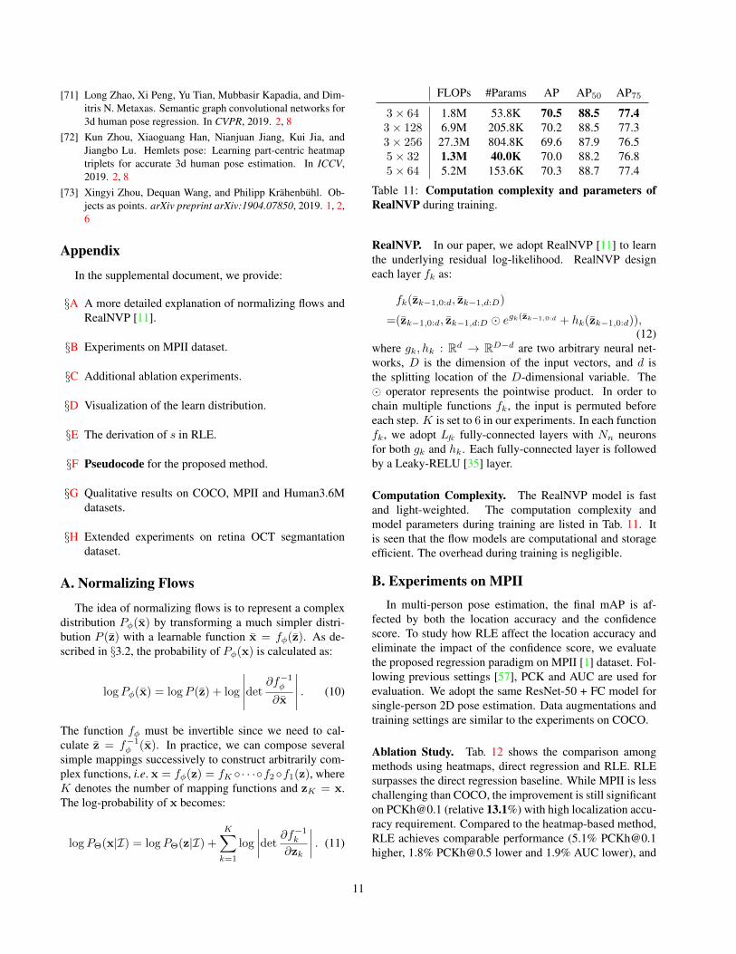
3× 64 1.8M 53.8K 70.5 88.5 77.43× 128 6.9M 205.8K 70.2 88.5 77.33× 256 27.3M 804.8K 69.6 87.9 76.55× 32 1.3M 40.0K 70.0 88.2 76.85× 64 5.2M 153.6K 70.3 88.7 77.4
Table 11: Computation complexity and parameters ofRealNVP during training.
RealNVP. In our paper, we adopt RealNVP [11] to learnthe underlying residual log-likelihood. RealNVP designeach layer fk as:
fk(zk−1,0:d, zk−1,d:D)
=(zk−1,0:d, zk−1,d:D � egk(zk−1,0:d + hk(zk−1,0:d)),(12)
where gk, hk : Rd → RD−d are two arbitrary neural net-works, D is the dimension of the input vectors, and d isthe splitting location of the D-dimensional variable. The� operator represents the pointwise product. In order tochain multiple functions fk, the input is permuted beforeeach step. K is set to 6 in our experiments. In each functionfk, we adopt Lfc fully-connected layers with Nn neuronsfor both gk and hk. Each fully-connected layer is followedby a Leaky-RELU [35] layer.
Computation Complexity. The RealNVP model is fastand light-weighted. The computation complexity andmodel parameters during training are listed in Tab. 11. Itis seen that the flow models are computational and storageefficient. The overhead during training is negligible.
B. Experiments on MPIIIn multi-person pose estimation, the final mAP is af-
fected by both the location accuracy and the confidencescore. To study how RLE affect the location accuracy andeliminate the impact of the confidence score, we evaluatethe proposed regression paradigm on MPII [1] dataset. Fol-lowing previous settings [57], PCK and AUC are used forevaluation. We adopt the same ResNet-50 + FC model forsingle-person 2D pose estimation. Data augmentations andtraining settings are similar to the experiments on COCO.
Ablation Study. Tab. 12 shows the comparison amongmethods using heatmaps, direct regression and RLE. RLEsurpasses the direct regression baseline. While MPII is lesschallenging than COCO, the improvement is still significanton [email protected] (relative 13.1%) with high localization accu-racy requirement. Compared to the heatmap-based method,RLE achieves comparable performance (5.1% [email protected], 1.8% [email protected] lower and 1.9% AUC lower), and
11
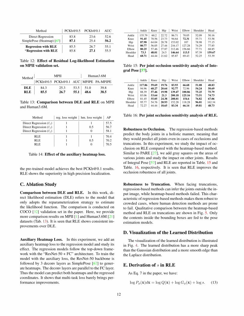
Method [email protected] [email protected] AUC
Direct Regression 83.8 23.6 52.6SimplePose (Heatmap) [67] 87.1 25.4 56.2
Regression with RLE 85.5 26.7 55.1*Regression with RLE 85.8 27.1 55.5
Table 12: Effect of Residual Log-likelihood Estimationon MPII validation set.
Method MPII Human3.6M
[email protected] [email protected] AUC MPJPE PA-MPJPE
DLE 84.3 25.3 53.5 51.0 39.8RLE 85.5 26.7 55.1 48.6 38.5
Table 13: Comparison between DLE and RLE on MPIIand Human3.6M.
Method reg. loss weight hm. loss weight AP
Direct Regression (`1) 1 1 57.5Direct Regression (`1) 1 0.5 56.7Direct Regression (`1) 1 0 58.1
RLE 1 1 70.4RLE 1 0.5 70.2RLE 1 0 70.5
Table 14: Effect of the auxiliary heatmap loss.
the pre-trained model achieves the best [email protected] results.RLE shows the superiority in high precision localization.
C. Ablation Study
Comparison between DLE and RLE. In this work, di-rect likelihood estimation (DLE) refers to the model thatonly adopts the reparameterization strategy to estimatethe likelihood function. The comparison is conducted onCOCO [32] validation set in the paper. Here, we providemore comparison results on MPII [1] and Human3.6M [21]datasets (Tab. 13). It is seen that RLE shows consistent im-provements over DLE.
Auxiliary Heatmap Loss. In this experiment, we add anauxiliary heatmap loss to the regression model and study itseffect. The regression models follow the top-down frame-work with the “ResNet-50 + FC” architecture. To train themodel with the auxiliary loss, the ResNet-50 backbone isfollowed by 3 deconv layers as SimplePose [67] to gener-ate heatmaps. The deconv layers are parallel to the FC layer.Thus the model can predict both heatmaps and the regressedcoordinates. It shows that multi-task loss barely brings per-formance improvements.
Ankle Knee Hip Wrist Elbow Shoulder Head
Ankle 135.79 60.2 22.72 86.71 70.05 52.09 50.16Knee 91.45 70.56 23.73 94.64 72.31 55.71 53.58Hip 87.98 64.04 28.78 153.02 107 78.98 77.15
Wrist 80.77 56.05 27.44 216.17 127.28 74.29 77.85Elbow 80.25 57.46 27.87 212.46 156.66 77.71 68.85
Shoulder 73.3 48.01 24.5 146.64 113.5 97.39 159.67Head 68.71 44.44 21.62 85.87 69.43 52.25 53.39
Table 15: Per joint occlusion sensitivity analysis of Inte-gral Pose [57].
Ankle Knee Hip Wrist Elbow Shoulder Head
Ankle 117.86 59.69 19.76 83.93 66.68 51.08 48.83Knee 94.96 68.27 20.64 92.77 72.96 54.24 50.69Hip 88.39 57.46 19.98 139.47 100.86 75.25 75.79
Wrist 83.06 53.64 21.3 200.18 125.16 73.51 74.73Elbow 81.45 55.05 24.38 208.01 154.6 76.82 67.06
Shoulder 95.77 54.76 20.93 152.28 118.28 96.01 162.34Head 72.27 44.44 18.65 83.34 66.14 49.81 48.73
Table 16: Per joint occlusion sensitivity analysis of RLE.
Robustness to Occlusion. The regression-based methodspredict the body joints in a holistic manner, meaning thatthey would predict all joints even in cases of occlusions andtruncations. In this experiment, we study the impact of oc-clusion on RLE compared with the heatmap-based method.Similar to PARE [27], we add gray squares on the areas ofvarious joints and study the impact on other joints. Resultsof Integral Pose [57] and RLE are reported in Table. 15 andTable. 16, respectively. It is seen that RLE improves theocclusion robustness of all joints.
Robustness to Truncation. When facing truncations,regression-based methods can infer the joints outside the in-put image, while heatmap-based methods failed. This char-acteristic of regression-based methods makes them robust tocrowded cases, where human detection methods are proneto fail. Qualitative comparison between the heatmap-basedmethod and RLE on truncations are shown in Fig. 5. Onlythe contents inside the bounding boxes are fed to the poseestimation models.
D. Visualization of the Learned Distribution
The visualization of the learned distribution is illustratedin Fig. 4. The learned distribution has a more sharp peakthan the Gaussian distribution and a more smooth edge thanthe Laplace distribution.
E. Derivation of s in RLE
As Eq. 7 in the paper, we have:
logPφ(x)dx = logQ(x) + logGφ(x) + log s. (13)
12
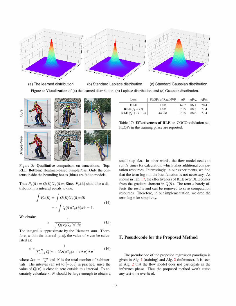
(a) The learned distribution (b) Standard Laplace distribution (c) Standard Gaussian distribution
Figure 4: Visualization of (a) the learned distribution, (b) Laplace distribution, and (c) Gaussian distribution.
Our
sS
impl
ePos
e
Figure 5: Qualitative comparison on truncations. Top:RLE. Bottom: Heatmap-based SimplePose. Only the con-tents inside the bounding boxes (blue) are fed to models.
Thus Pφ(x) = Q(x)Gφ(x)s. Since Pφ(x) should be a dis-tribution, its integral equals to one:
∫Pφ(x) =
∫Q(x)Gφ(x)sdx
= s
∫Q(x)Gφ(x)dx = 1.
(14)
We obtain:s =
1∫Q(x)Gφ(x)dx
. (15)
The integral is approximate by the Riemann sum. There-fore, within the interval [a, b], the value of s can be calcu-lated as:
s ≈ 1∑Ni=1Q(a+ i∆x)Gφ(a+ i∆x)∆x
, (16)
where ∆x = b−aN and N is the total number of subinter-
vals. The interval can set to [−5, 5] in practice, since thevalue of Q(x) is close to zero outside this interval. To ac-curately calculate s, N should be large enough to obtain a
Loss FLOPs of RealNVP AP AP50 AP75
DLE 1.8M 62.7 86.1 70.4RLE (Q+G) 1.8M 70.5 88.5 77.4
RLE (Q+G+ s) 44.2M 70.5 88.6 77.4
Table 17: Effectiveness of RLE on COCO validation set.FLOPs in the training phase are reported.
small step ∆x. In other words, the flow model needs torun N times for calculation, which takes additional compu-tation resources. Interestingly, in our experiments, we findthat the term log s in the loss function is not necessary. Asshown in Tab. 17, the effectiveness of RLE over DLE comesfrom the gradient shortcut in Q(x). The term s barely af-fects the results and can be removed to save computationresources. Therefore, in our implementation, we drop theterm log s for simplicity.
F. Pseudocode for the Proposed Method
The pseudocode of the proposed regression paradigm isgiven in Alg. 1 (training) and Alg. 2 (inference). It is seenin Alg. 2 that the flow model does not participate in theinference phase. Thus the proposed method won’t causeany test-time overhead.
13
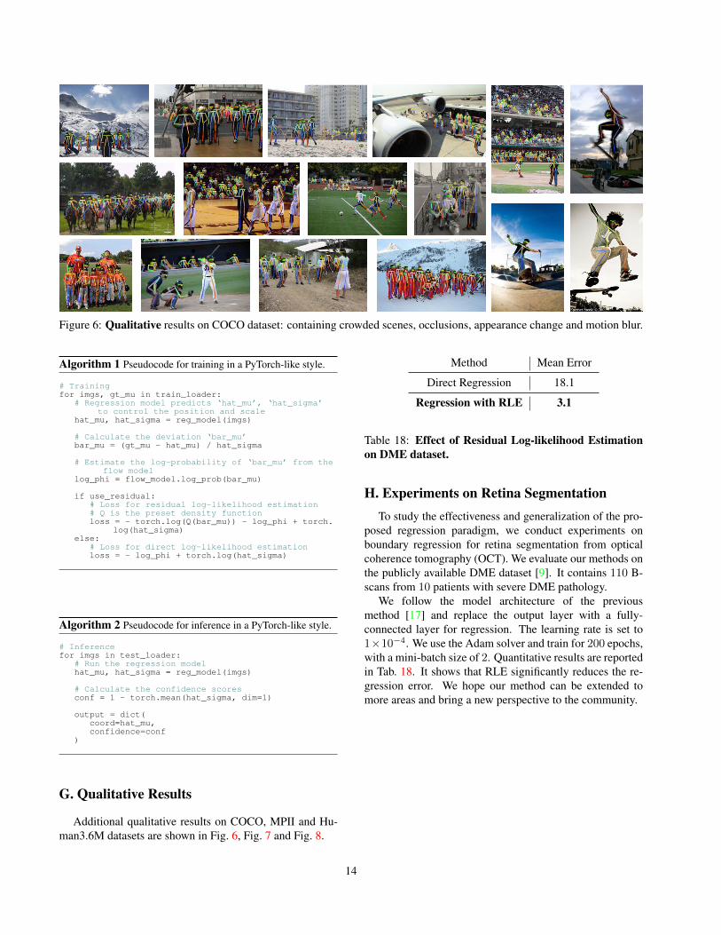
Figure 6: Qualitative results on COCO dataset: containing crowded scenes, occlusions, appearance change and motion blur.
Algorithm 1 Pseudocode for training in a PyTorch-like style.
# Trainingfor imgs, gt_mu in train_loader:
# Regression model predicts ‘hat_mu’, ‘hat_sigma’to control the position and scale
hat_mu, hat_sigma = reg_model(imgs)
# Calculate the deviation ‘bar_mu’bar_mu = (gt_mu - hat_mu) / hat_sigma
# Estimate the log-probability of ‘bar_mu’ from theflow model
log_phi = flow_model.log_prob(bar_mu)
if use_residual:# Loss for residual log-likelihood estimation# Q is the preset density functionloss = - torch.log(Q(bar_mu)) - log_phi + torch.
log(hat_sigma)else:
# Loss for direct log-likelihood estimationloss = - log_phi + torch.log(hat_sigma)
Algorithm 2 Pseudocode for inference in a PyTorch-like style.
# Inferencefor imgs in test_loader:
# Run the regression modelhat_mu, hat_sigma = reg_model(imgs)
# Calculate the confidence scoresconf = 1 - torch.mean(hat_sigma, dim=1)
output = dict(coord=hat_mu,confidence=conf
)
G. Qualitative Results
Additional qualitative results on COCO, MPII and Hu-man3.6M datasets are shown in Fig. 6, Fig. 7 and Fig. 8.
Method Mean Error
Direct Regression 18.1
Regression with RLE 3.1
Table 18: Effect of Residual Log-likelihood Estimationon DME dataset.
H. Experiments on Retina SegmentationTo study the effectiveness and generalization of the pro-
posed regression paradigm, we conduct experiments onboundary regression for retina segmentation from opticalcoherence tomography (OCT). We evaluate our methods onthe publicly available DME dataset [9]. It contains 110 B-scans from 10 patients with severe DME pathology.
We follow the model architecture of the previousmethod [17] and replace the output layer with a fully-connected layer for regression. The learning rate is set to1×10−4. We use the Adam solver and train for 200 epochs,with a mini-batch size of 2. Quantitative results are reportedin Tab. 18. It shows that RLE significantly reduces the re-gression error. We hope our method can be extended tomore areas and bring a new perspective to the community.
14
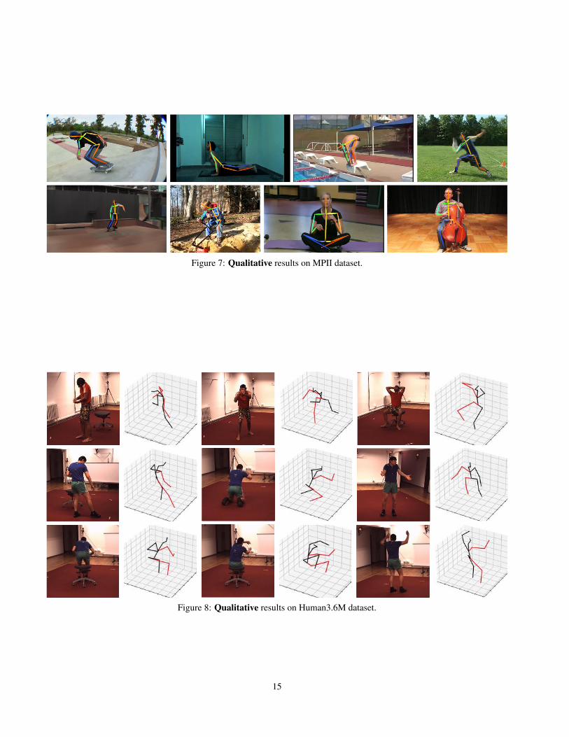
Figure 7: Qualitative results on MPII dataset.
Figure 8: Qualitative results on Human3.6M dataset.
15

![Test-time Adaptation for 3D Human Pose Estimation3D [1,4,5,12]. In these approaches 2D detectors are either used to model the likelihood of the 3D pose [5,12], or provide a set of](https://img.pdfslide.net/doc/110x75/5fe817978875942258299736/test-time-adaptation-for-3d-human-pose-estimation-3d-14512-in-these-approaches.jpg)