Huxley’s Model of Muscle Contraction with · PDF fileHuxley’s Model of Muscle Contraction with Compliance W. O. Williams January 3, 2011 Abstract Huxley’s cross-bridge dynamics

Huxley’s Model of Muscle Contraction withCompliance

W. O. Williams

January 3, 2011

Abstract

Huxley’s cross-bridge dynamics of muscle contraction is widely usedin understanding, in particular, laboratory experiments on muscles andsubunits of muscle. The hard-connection version of the model has severaldefects. In this paper I present a detailed and precise method of solutionof the problem with a compliant element in series with the muscle.

1 Introduction

The Huxley [4] model of muscle contraction, formulated more than fifty yearsago, still is the model most used by experimenters. This fact reflects both thesimplicity of the model and the inability of more elaborate models simultane-ously to replicate its precision on the basic experimental tests and to apply suc-cessfully to more than a single extended test.

The formulation is a simple population-dynamics model, with elementaryaffine birth- and death-rate rules and a linear elastic mechanics for force gener-ation. Various proposals to “tweak” the system by altering these rules have notgreatly improved its predictive ability, in particular not repairing defects in itspredictions (including those noted by Huxley himself).

One aspect of the Huxley model which hampers its performance is that it is a“hard” system, with rigid attachment of the force-generating element to attach-ment points. Of course all physiologists recognize the elasticity of tendon andthe microscopic fibers within the muscle itself, and a few adjusted models haveappeared in the literature. In this paper, I derive the equations which describethe system with an added serial elastic element and give a formal integrationscheme for them. I present computations to verify that the equations can pre-dict two classical experimental results not within the scope of the original forms.

1

Compliant Huxley Model January 3, 2011 Page 2 of 22

FascicleFiber

Myofibril

Figure 1: An illustration of the structure of a skeletal muscle

2 Physiology and Experiments

Figure 1 illustrates the base structure of skeletal (striated) muscle, as observedsince the invention of the light microscope. The remarkable fact which enablesextension of calculations from molecular level to (nearly) whole muscle is theregularity of the structure. Each muscle is comprised of a collection of fascicles,usually laid in a parallel arrangement, and each of these fascicles is a bundleof muscle fibres likewise laid in a parallel arrangement. To have a sense of scale:the fibres, each of which is a single cell, may be 10-100µ in diameter, while beingas much as 30 cm long. There may be 100,000 fibres in a muscle. The regularityof structure extends to the next level as well. As sketched, each fibre includes abundle of a hundred or more myofibrils, approximately 1-3 µ in diameter. Themyofibrils, as illustrated, have a banded appearance, leading to the descriptionof skeletal muscle as striated muscle. This regular striation consists in periodicstructures called sarcomeres (Figure 2).

Each sarcomere is about 2.5 µ long and is symmetric. Within the sarcom-ere there are, as indicated, filaments,which are coiled collections of polymericchains of molecules. The thicker ones are myosin; the regular array of thick fil-aments is interleaved in a regular geometric pattern with thin filaments of actinmolecules, each thick filament surrounded by six thin ones. The myosin fila-ments are anchored at each end of the sarcomere; the actin filaments are at-tached together by a membrane in the center. The thick filaments are approxi-


Myofibril

Myosin Actin

Sarcomere

Actin Lattice

MyosinLattice Anchoring Intermeshed

Lattices

Figure 2: The sarcomere.

mately 15 nm in diameter, the thin ones about 6 nm. Because of the symmetry ofthe sarcomere, the computational unit which we consider is the half-sarcomere.

Contraction of the muscle is effected by sliding of the thin and the thick fil-aments past one another. The mechanism that engenders this sliding action isnow agreed to be the action of the myosin cross-bridges. Each myosin moleculeconsists of a long thin tail with a pair of globular heads. About 180 of thesemolecules are coiled together to form a thick filament with the heads and theleading part of the tail projecting from the coil to form a cross-bridge. The headsinclude a binding site for actin, and a site which accepts adenosine triphos-phate, or ATP, molecules. The thin filament, in turn, consists of two polymericchains of actin in a helical coil which presents spaced binding sites for the myosin.

When the muscle is stimulated, in vivo through the presence of Ca2+ ionsperfusing the sarcomere and unblocking binding sites on the actin filament, thecross-bridge head attaches to the adjacent thin filament. At this point hydroliza-tion of an attached ATP molecule (which loses a phosphate and becomes aden-esine diphosphate or ADP) creates a change in angle of the myosin head relativeits tail, and the result is a shift of the cross-bridge head’s pivot point relative thethin filament. At the end of the process the myosin head detaches (with anotherATP–ADP reaction).

The angular shift can have two results (or a combination of the two) in that


the thin filaments may slide past the thick ones, or, if constrained from so do-ing, the shift stretches the elastic cross-bridge tail (and the compliant actin andmyosin filaments). The stretching generates the force which the muscle exerts,while the sliding generates the contraction of the muscle.

Modeling of the behavior of larger units, filament, fascicle or whole muscle isdeduced from the behavior of sarcomeres, due to the regular arrangement of theelements, since it is usually held that the stimulation is essentially simultaneousthroughout the muscle. The parallel arrangement of fibrils leads to additivityof forces across the cross-section, extending to the entire muscle. Likewise, theconcatenation of sarcomeres engenders additivity of length, and hence additiv-ity of velocity along the length of a fibre. That neither additivity is absolutelytrue in detail has been observed1, but in any case additivity seems a reasonableassumption.

There are several classical experiments which serve as benchmarks for anyproposed model. We look at the ones which are most relevant to our purposeshere.

A twitch is the result of a single pulse of stimulation applied to a muscle.Normally the experiment is done with the muscle held at fixed length and theresulting force measured. The force ascends to a peak value and then decays tozero.

A tetanus is the result of a sustained stimulation. Again the standard exper-iment has the muscle held at fixed length, with force measured. A typical trace,with a twitch of the same muscle, is shown in Figure 3,

A later result is important to us: experiments show that in a tetanus, theforce evolution toward its maximum lags behind the evolution of the number ofattached cross-bridges. (The latter is deduced from measurements of the evo-lution of the stiffness of the muscle.) This lagging of force is contrary to the pre-dictions of the simplest version of the Huxley model.

3 Basics of Huxley’s Model.

In 1957 A. E. Huxley [4] developed the base model which has proved the founda-tion for all subsequent work, including elaborations which he shared in creating.Here we examine the ideas basic to this model. It is important to note that thismodel pre-dates the notion of rotation of the myosin heads; in fact, at the time itwas considered debatable even that the cross-bridges were the actors in gener-

1Perreqault et al [32] find non-additivity of force. It has long been suggested that lengthchanges may not be uniform along the muscle; see, e.g., Sugi and Kobayashi [10], See also thediscussion by Zajac [15].


0 100 200 300 400 5000.0

0.2

0.4

0.6

0.8

Time (msec)

Forc

e (n

orm

alize

d)

Figure 3: Tetanus and twitch traces superposed, using data from [30] .

ating the relative sliding of the two classes of fibers; Huxley proposed the modelto aid in validating this concept2.

Consider a half-sarcomere. Huxley pictured the myosin heads, attached tothe parent myosin filament by elastic tails, by utilizing a cartoon replicated inFigure 4. When the muscle is stimulated, those heads which are in the vicin-ity of an attachment site on the actin filament can be expected to attach to thatsite. Force then would be applied to the actin filament by the stretched elastictail of the cross-bridge; a contractile force being created if the elastic tail is in astate of extension. Since a contraction velocity would tend to shorten the elas-tic tail, in order that force be created one must suppose that the cross-bridgetail already is extended when the cross-bridge attaches. Huxley proposed thatthis extension could be provided by thermal agitation of the cross-bridge head.Since this agitation should be as likely to contract as to extend the tails of in-dividual cross-bridges, Huxley further suggested that attachment would, by anunspecified chemo-mechanical mechanism, be facilitated for the cross-bridgeswhich are displaced positively and made difficult for those whose tails are in a

2The cross-bridge-generated sliding-filament model was not universally accepted until the in-vention of the electron microscope enabled direct observation.


Actin

Myosin

x

v

Contraction of Muscle

Figure 4: Huxley’s basic cartoon

rest position or contracted.3

The variable of significance for the problem is the displacement x. Basedthen on the enormous numbers of cross bridges involved, it is reasonable tomodel the number of cross-bridges as a distribution in x. The number of cross-bridges which are attached to the actin filament at time t and which have dis-placement between a and b is

N ((a,b), t ) =∫ b

an(x, t )dx , (1)

and the total number attached is

N (t ) =∫ X

−Xn(x, t )dx , (2)

where X is the maximum possible extension of the cross-bridge tail.The balance relation for numbers of cross-bridges in the interval (a,b) will

involve an attachment rate F (x, t ) and a detachment rate G(x, t ) and also trans-port effects, as the velocity of contraction, in drawing the actin filament past themyosin filament, will carry cross-bridges into and out of this range of extension.We suppose that both F and G are piecewise continuous and of compact sup-port. Then we have

d

d tN ((a,b), t ) =

∫ b

a

∂n

∂t(x, t )dx

=∫ b

a(F (x, t )−G(x, t )) dx + v(t )[n(b, t )−n(a, t )] . (3)

3Huxley recognized the ad hoc nature of these suppositions, and ultimately revised the model.


The signs on the latter terms reflect the fact that the velocity of contractionv(t ) carries cross-bridges with a certain displacement into smaller values of dis-placement. If we divide this equation by b−a and take the limit as b approachesa, we obtain the equation of balance of cross-bridges:

∂n(x, t )

∂t= F (x, t )−G(x, t )+ v(t )

(∂n(x, t )

∂x

)or

∂n(x, t )

∂t− v(t )

(∂n(x, t )

∂x

)= F (x, t )−G(x, t ) (4)

The natural associated initial condition would be

n(x,0) = no(x). (5)

Following the Huxley cartoon, each attached cross-bridge provides a forceaccording to the extension imposed upon the cross-bridge’s tail section. Sup-posing that the response is elastic 4, we arrive at the form

P (t ) =∫ X

−XE (x)n(x, t )dx . (6)

Here P (t ) is the tension of the muscle, and we suppose E to be an non-decreasingfunction, zero at x = 0. It seems to be most consistent with the physical modelto suppose that negative values of x should produce no compressive force, al-though compressive forces are allowed in some elaborations of the model.

Although it is generally recognized that biological materials are genericallynon-linear in response, Huxley, and most of the developers of his model up tothe current time, assume the elasticity in the myosin tails to be linear. In part,this is justified by convenience and in part by recognition that in light of the largenumbers involved an averaged elasticity may be appropriate.

Two steps remain before we introduce the particular constitutive equationsof the Huxley 1957 model.

First, it is natural to simplify the form of the computations by normalizingthe distribution functions. In light of the parallel nature of the structures, scal-ing upwards by the number of cross-bridges in an assembly then is quite simple.While it seems natural to normalize by dividing the density n(x, t ) by the total

4It has long been recognized that biological materials, and in particular, polymers like the actinfilaments, display more elaborate behaviors (see, e.g., [37]), in particular, both rate-dependenceand some memory effects.


number of cross-bridges available, in order to justify the linearization in the up-take and loss functions which is assumed by Huxley and all elaborators of hismodel, one should divide n(x, t ) by the total number of cross-bridges availableat the extension x. Implicitly, Huxley and the others assume that the total popu-lation of cross-bridges at extension x, U (x, t ), is a constant, independent of bothx and t 5. Let this constant be U ; we define a new density

w(x, t ) = n(x, t )

U. (7)

and rewrite the balance equation:

∂w(x, t )

∂t− v(t )

(∂w(x, t )

∂x

)= F (x, t )

U− G(x, t )

U(8)

Second, we note that it is convenient for analysis and computation to use arestatement of the problem by using characteristic coordinates. We define

χ(r, t ) := r −∫ t

0v(s)ds =: r −R(t ) (9)

so that r is a virtual reference displacement: one pictures r = constant as identi-fying a cross-bridge attached and of length r at time 0 so that χ tracks its historyas time goes on. We use (9) to change coordinates via

σ(r, t ) := w(χ(r, t ), t ) , (10)

so that, for example, the total number of attached cross-bridges can be expressedas

N (t ) =U∫ ∞

−∞σ(r, t )dr ; (11)

of course the support of σ(·, t ) is finite. This enables us to rewrite (4) as

∂σ

∂t(r, t ) = F (χ(r, t ), t )

U− G(χ(r, t ), t )

U. (12)

In his original article, Huxley chose to model the attachment and detach-ment rates for cross-bridges as

F (x, t )

U= (1−w(x, t )) f (x) (13)

and

G(x, t )

U= g (x) w(x, t ) (14)


f g

h

Figure 5: Huxley’s attachment and detachment functions

He took f and g to be of the forms shown in Figure 5; note that f is zero outsidethe interval [0,h] while g continues indefinitely.

Huxley said that he assumed f (x) and g to be linear in positive displacementx merely to simplify the analysis. The presence of the sharp limits on attachmentrate, 0 and h, represent the idea that attachments which would work againstthe acceleration of the motion are blocked, and that the extension of the cross-bridge tail is limited while the cross-bridge is unattached6. We presume thath ≤ X . Setting the detachment rate to be very high when the cross-bridge tailsare forced into a negative extension is a soft version of a stripping rule. Growth ofg with positive extension reflects a susceptibility of cross-bridges to detachmentwhen they are over-extended

Huxley’s 1957 version of the balance equation (8) then is

∂σ

∂t(r, t ) = f (χ(r, t ))− [

f (χ(r, t ))+ g (χ(r, t ))]σ(r, t ) ,

σ(r,0) = w0(r ) .

(15)

Finally, to replicate Huxley’s calculations, we assume that the cross-bridgetails are linearly elastic, so that the form of the force function now is

P (t ) =U Em

∫ X

−Xxw(x, t )dx =U Em

∫ ∞

−∞χ(r, t )σ(r, t )dr . (16)

5That this is necessary to ensure consistency apparently first was noted by Keener andSneyd[38], cf.[34].

6While h is thus proposed as the the maximal “natual” extension of a cross-bridge, it is not amaximum for extension, since a cross-bridge may be displaced further through a forced exten-sion.


A

D

C

B

t

rh0

F

E

Figure 6: Characteristics (dashed lines) in the r − t plane.

Note that a uniform delta-function increment in displacement would produce adelta-function increment in tension of

U Em

∫ X

−Xw(x, t )dx = N (t )Em , (17)

yielding an instantaneous modulus of elasticity of the contractile unit.To obtain explicit or easily computable solutions, we formally integrate the

balance equation (15). Consider the r − t plane as shown in Fig 6. If we supposethat v always is positive, then R as defined in (9) is invertible and the graphsof r = R(t ) and r = h +R(t ) might look like those plotted as dashed lines. Thevertical bars and these section the plane into the domains A, B, C, D, E and F,with slightly different formulae applying in each.

In A, D and F we have x ≤ 0 and thus solve

∂σ(r, t )

∂t=−g2σ(r, t ) (18)

yielding

σ(r, t ) = K (r )exp{−g2t

}. (19)

The initial condition, and hence K (r ), differs from region to region.In B and E we have 0 ≤ x ≤ h, so that we solve

∂σ(r, t )

∂t= f1χ(r, t )− [

f1 + g1]χ(r, t )σ(r, t ) (20)


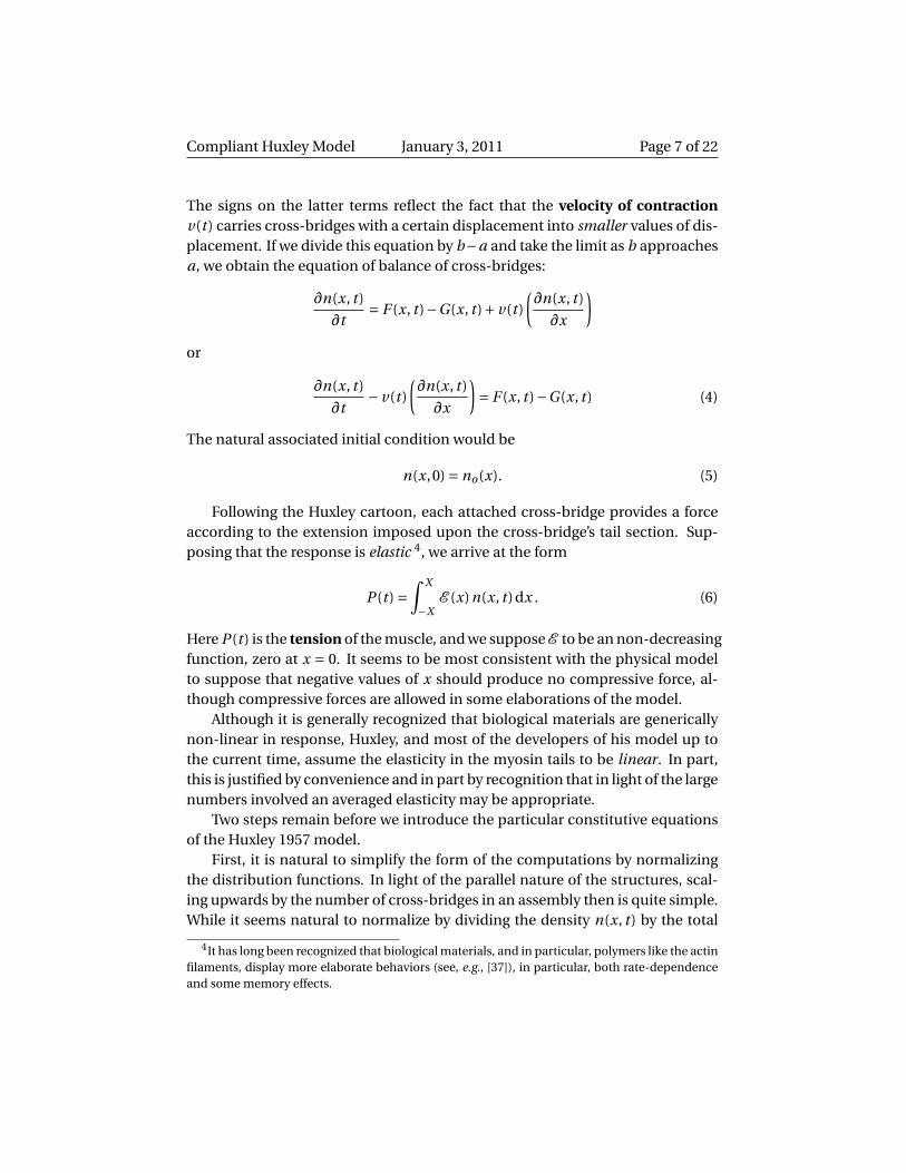
yielding

σ(r, t ) = f1

∫ t

0

[χ(r, s)exp

{−( f1 + g1)

∫ t

sχ(r,τ)dτ

}]ds

+K (r )exp

{−( f1 + g1)

∫ t

0χ(r, s)ds

}. (21)

Again, the initial condition differs between the two regions.In C we solve

∂σ(r, t )

∂t=−g1χ(r, t )σ(r, t ) (22)

yielding

σ(r, t ) = w0(r )exp

{−g1

∫ t

0χ(r, s)ds

}. (23)

Here the initial condition is σ(r,0) = w0(r ).Finally, we can express the solutions by matching across the region bound-

aries. We note that the upper curve of separation can be expressed as

t = T (r ) = R−1(r ) (24)

and the lower as

t = T1(r ) = R−1(r −h) (25)

Then we work upwards to establish

σA(r, t ) = w0(r )exp{−g2t

}, (26a)

σB (r, t ) = f1

∫ t

0

[χ(r, s)exp

{−( f1 + g1)

∫ t

sχ(r,τ)dτ

}]ds

+w0(r )exp

{−( f1 + g1)

∫ t

0χ(r, s)ds

}, (26b)

σC (r, t ) = w0(r )exp

{−g1

∫ t

0χ(r, s)ds

}, (26c)

σD (r, t ) =σB (r,T (r ))exp{−g2 (t −T (r ))

}, (26d)

σE (r, t ) = f1

∫ t

T1(r )

[χ(r, s)exp

{−( f1 + g1)

∫ t

sχ(r,τ)dτ

}]ds

+σC (r,T1(r ))exp

{−( f1 + g1)

∫ t

T1(r )χ(r,τ)dτ

}, (26e)


and

σF (r, t ) =σE (r,T (r ))exp{−g2 (t −T (r ))

}. (26f)

We eschew the straightforward expression for the corresponding tensions, as be-ing non-informative.

4 Serial Elasticity

The above model reflects the historical form up until 1969, in that it allowedfor elasticity in the system only in the cross-bridge tails. From the beginningit was recognized that the upwardly scaled full muscle model should be cor-rected for the elasticity of the attaching tendons. The elasticity of the thick andthin filaments and the other attaching structure in the sarcomere likewise wasnominally acknowledged but usually it was supposed, if only for conveniencein modeling, that the contribution of the stretch of the filaments was negligiblecompared to that of the cross-bridges. Only in 1994, after experiments ([17] and[19]) confirmed that only 30 to 50% of the compliance of the filament should beascribed to the cross-bridge tails did this attitude begin to change.

Introducing this contribution in the Huxley model is important. A) If the at-tachment rate of the cross-bridges depends upon the number of myosin headsat a given extension which find themselves adjacent to a binding site on the actinfiber, the probabilities of attachment must change with tension, since the elasticstretch of the thin and thick filaments must differ. B) There are purely mechan-ical effects. First, the long-standing way of determining the elastic modulus ofthe cross-bridge tails is through experiments measuring the force response assuper-posed small extensions are applied to tetanically-contracting muscles. Ifpart of the measured deformation is due to elasticity of the filaments, then theprevious estimates of elasticity of the cross-bridge tails would have been lowerthan actually was true, and in turn this would cause inaccuracies in predictionsof response in other experiments. Similarly, once the cross-bridge-tail elasticmodulus has been deduced, the most convenient way to determine evolutionof the numbers of cross-bridges attached at a given time in an experiment is tomeasure the force response under such super-posed extensions of the muscle.If the elasticity were all in the cross-bridges, the force would be proportional tothe number attached, if not, as we see below, this proportionality fails. Finally,the filament elasticity must contribute to the form of the force-time curve in atime-varying experiment, as during an excitation or relaxation or during a forcedmovement.


Direct inclusion of the kinetic effect A) is naturally done through change ofthe attachment and detachment rules F and G , or in more elaborate multi-statekinetics through change in the kinetic coefficients. Most of the literature oncompliance effects focuses on this aspect. Here we will consider the mechan-ical effect B), retaining the original Huxley kinetics. The bibliography includesarticles treating both effects, but here we discuss only those which include sig-nificant discussion of the mechanical effects.

In 1969 Julian [5] did calculations with a truncated Huxley model, includinga non-linear elastic element in series with the contractile element. He also intro-duced a time-course excitation for tetanus and twitch. Following the 1994 exper-iments, Goldman and Huxley [16] did rough computations overlying the model,extended somewhat in 1996 by Huxley and Tideswell [21]. Using a discretizedversion of the model in 1993 and 1994 Luo, Cooke and Pate [?, 18] consideredthe effect of series compliance on decay of tetanus and on the lead-lag prob-lem discussed below. In 1996 Mijailovich, Fredberg and Butler [22] considereda detailed model with elasticity in both actin and myosin, decoupling the equa-tions of deformation from the cross-bridge kinetics to obtain computations ofthe lead-lag problem similar to those below. Torelli in 1997 [24] established ex-istence and uniqueness for the fully coupled Huxley-kinetics, elastic actin prob-lem with rather general constitutive equations.

Here we integrate the standard Huxley model with an added series linearelasticity to illustrate the effect of non-cross-bridge elasticity7. We thus can usethe integrated density equations (26), but need to reexamine the evolution of thedisplacement.

Let L+l (t ) denote the total length of the muscle/series-elastic element, withl (0) = 0. If the length of the series-elasticity element is ls(t ) and that of the con-tractile unit lm(t ), we have

l ′s(t )+ l ′m(t ) = l ′(t ). (27)

The contraction velocity of the muscle then is

v(t ) =−l ′m(t ) = l ′s(t )− l ′(t ) (28)

The length of the elastic unit, or spring, is determined by the tension generatedby the muscle, and hence carried by the elastic unit, as

ls(t )−Ls = P (t )/Es ; (29)

7The elaboration which includes detailed actin and myosin elasticity does not lead to improve-ments in the output.


where Ls is the rest-length of the spring and Es its modulus of elasticity8. From(28) we have a relation between the cross-bridge extension and the force in thespring:

χ(r, t ) = r −∫ t

0v(s)ds = r −

(ls(t )− ls(0)

)+ l (t )

= r − 1

Es

(P (t )−P (0)

)+ l (t ) (30)

Now we combine (30) and (16), the representation for P (t ), to find

χ(r, t ) = r −(

U Em

Es

) [∫ ∞

−∞χ(p, t )σ(p, t )dp −

∫ ∞

−∞pw0(p)dp

]+ l (t ) . (31)

Here we recall the notation w0 for the initial distribution of attached cross-bridges.To simplify calculations, let us set

µ= U Em

Es, (32)

Q(t ) =∫ ∞

−∞σ(p, t )dp , (33)

M(t ) =∫ ∞

−∞χ(p, t )σ(p, t )dp . (34)

In light of (17), µ is the ratio of a “maximal” elastic modulus of the contractileunit to the elastic modulus of the serial unit; UQ(t ) is the number of attachedcross-bridges.

Using these abbreviations, (31) is

χ(r, t ) = r −µ(M(t )−M(0)

)+ l (t ) (35)

We multiply through by σ(r, t ) and integrate to obtain

M(t ) =∫ ∞

−∞rσ(r, t )dr −µ [M(t )−M(0)]Q(t )+ l (t )Q(t ) , (36)

and solve to find

M(t )−M(0) =[∫ ∞

−∞rσ(r, t )dr −M(0)+ l (t )Q(t )

]/(1+µQ(t )) . (37)

8To facilitate comparison to the previous results for the Huxley57 model, we assume linearelastic response for the series unit and for the elasticity of the cross-bridges. Changing to non-linear elastic forms leads to obscuring complexity


Finally, then, we obtain the prescription for the displacement

χ(r, t ) = r − µ

1+µQ(t )

∫ ∞

−∞(σ(p, t )−w0(p)

)p dp + l (t )

1+µQ(t ). (38)

We now can use (38) to calculate χ for the formal solutions (26), and alsoto determine the region boundaries in Fig 6 for the current case. In practice, itis necessary to calculate numerically. The results shown below are found by afront-tracking scheme: the fronts in the r − t plane are those where the attach-ment and detachment functions change form: χ(r, t ) = 0 and χ(r, t ) = h. Giventhese r values at a specified time, we project them forward for a time-step, usingthe current velocity. Then the resulting values ofσ at the new time are calculatedfrom (26). These values are then used to find a new χ, from (38) and the processcontinued.

Isometric Loading; Tetanus and TwitchIn this instance l (t ) = 0 and the initial density of attached cross-bridges is

assumed to be zero. Computations were made for various values of the compli-ance ratio

µ= U Em

Es. (39)

The computation for µ= 0 corresponds to rigid attachments of the muscle unitand increasing values of µ describe increasing compliance in the serial element.

The first set of computations is to verify that the presence of serial compli-ance changes the timing of the number and tension development in a tetanus.In Figure 7, graphing normalized values of both quantities, we see that at a valueof µ = 0 (original Huxley model), the tension does lead the number, while withserial compliance, hereµ= 10, the precedence is reversed. It also is worth notingthat the presence of compliance significantly delays the development of bothnumber and tension. The point at which lead becomes lag is on the order ofµ= 2.

These computations show that contrary to some conjectures in the litera-ture, the shift in tension-number development can be the effect simply of serialcompliance.

As pointed out above, however, the experimentalists compare instead theevolution of the tension and the stiffness (modulus of elasticity) of the muscle9.

9To examine the stiffness experimenters apply very high frequency superposed extensions (cf.,e.g., [26]).


0 200 400 6000.0

0.4

0.8

1.2

time (msec)

norm

aliz

ed v

alue

s

numbertension

0 200 400 6000.0

0.4

0.8

1.2

time (msec)

norm

aliz

ed v

alue

s

numbertension

Figure 7: Predictions of development of (normalized) number and tension, with-out (upper graph) and with serial compliance (µ= 10)


0 200 400 6000.0

0.4

0.8

1.2

time

norm

aliz

ed v

alue

s

stiffnesstension

0 200 400 6000.0

0.4

0.8

1.2

time

norm

aliz

ed v

alue

s

stiffnesstension

Figure 8: Predictions of development of (normalized) stiffness and tension,without (upper graph) and with serial compliance (µ= 3)

To examine this we combine (16) and (37) to obtain

P (t ) =U Em

{M(0)+

[∫ ∞

−∞rσ(r, t )dr −M(0)

]/(1+µQ(t ))

}+U Em

Q(t )

1+µQ(t )l (t ) (40)

Thus the modulus of elasticity in an increment of length is U EmQ(t )

1+µQ(t ) . Thenormalized values of this quantity are plotted together with the tension in Figure8. Again, the change from leading to lagging occurs, notably at a much lowervalue of µ (here the breaking point is µ= 0.5).

Next we turn to the effect of compliance on a twitch. Hill in [2] produceda series of twitches on the same muscle, first with rigid attachments, then with


0.0 0.1 0.2 0.30

2

4

6

time (sec)

forc

e

0.0 mm/10g0.440.691.042.58

0 20 400.00

0.05

0.10

0.15

0.20

time (msec)

forc

e

μ = 0.01.05.010.0

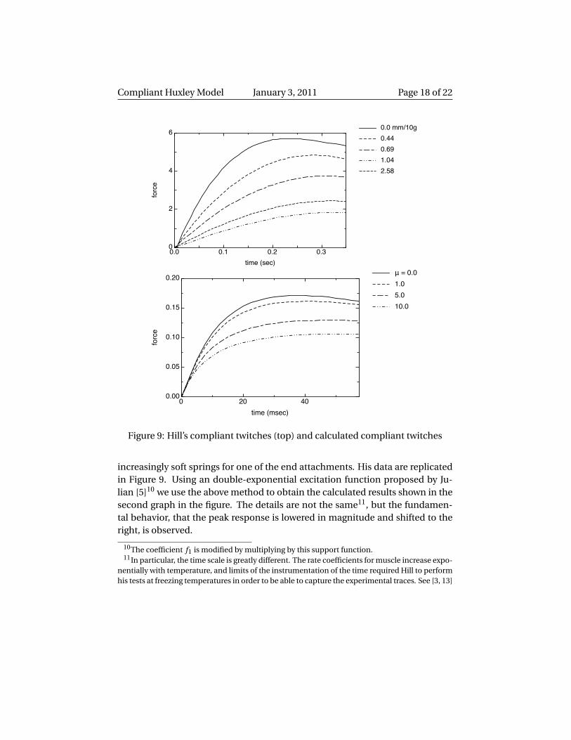
Figure 9: Hill’s compliant twitches (top) and calculated compliant twitches

increasingly soft springs for one of the end attachments. His data are replicatedin Figure 9. Using an double-exponential excitation function proposed by Ju-lian [5]10 we use the above method to obtain the calculated results shown in thesecond graph in the figure. The details are not the same11, but the fundamen-tal behavior, that the peak response is lowered in magnitude and shifted to theright, is observed.

10The coefficient f1 is modified by multiplying by this support function.11In particular, the time scale is greatly different. The rate coefficients for muscle increase expo-

nentially with temperature, and limits of the instrumentation of the time required Hill to performhis tests at freezing temperatures in order to be able to capture the experimental traces. See [3, 13]


References

[1] A. V. Hill. The heat of shortening and the dynamic constants of muscle.Proc. R. Soc. Lond. B, 126:136–195, 1938.

[2] A. V. Hill. The effect of series compliance on the tension developed in amuscle twitch. Proc. R. Soc. Lond. B, 138:325–329, 1951.

[3] A. V. Hill. The influence of temperature on the tension developed in anisometric twitch. Proc. R. Soc. Lond. B, 138:349–354, 1951.

[4] A. F. Huxley. Muscle structure and theories of contraction. Prog. Biophys.Biophys. Chem., 7:255–318, 1957.

[5] F. Julian. Activation in a skeletal muscle contraction model with a modifi-cation for insect fibrillar muscle. Biophys. J., 9:547–570, 1969.

[6] J. Thorson and D. C. S. White. Distributed representations of actin-myosininteraction in the oscillatory contraction of muscle. Biophys. J., 9:360–389,1969.

[7] A. F. Huxley and R. M. Simmons. A quick phase in the series-elastic com-ponent of striated muscle, demonstrated in isolated fibres from the frog. J.Physiol., 208:52P–53P, 1970.

[8] G. I. Zahalak. A distribution-moment approximation for kinetic theories ofmuscular contraction. Math. Biosci., 55:89–114, 1981.

[9] G Cecchi, P. J. Griffiths, and S. Taylor. Muscular contraction: Kineticsof crossbridge attachment studied by high-frequency stiffness measure-ments. Science, 217:70–72, 1982.

[10] H. Sugi and T. Kobayashi. Sarcomere length and tension changes intetanized frog muscle fibers after quick stretches and releases. Proc. Natl.Acad. Sci., 80:6422–6425, 1983.

[11] G. Avanzolini and A. Cappello. The characteristic method applied to thestudy of muscle dynamics. Bul. Math. Biol., 46:827–844, 1984.

[12] W. O. Williams. On the Lacker-Peskin model for muscular contraction.Math. Biosci., 70:203–216, 1984.

[13] A. F. Bennett. Temperature and muscle. J. Exp. Biology, 115:333–344, 1985.


[14] M. A. Bagni, G. Cecchi, and M. Schoenberg. A model of force productionthat explains the lag between crossbridge attachment and force after elec-trical stimulation of striated muscle fibers. Biophys. J., 54:1105–1114, 1988.

[15] F. E. Zajac. Muscle and tendon: properties, models, scaling, and applica-tions to biometrics and motor control. Crit. Rev. in Biomed. Eng., 17:359–411, 1989.

[16] Y. E. Goldman and A. F. Huxley. Actin compliance: are you pulling mychain? Biophys. J., 67:2131–2133, 1994.

[17] H. E. Huxley, A. Stewart, H. Sosa, and T. Irving. X-ray diffraction mea-surements of the extensibility of actin and myosin filaments in contractingmuscle. Biophys. J., 67:2411–2421, 1994.

[18] Y. Luo, R. Cooke, and E. Pate. Effect of series elasticity on delay in develop-ment of tension relative to stiffness during muscle activation. Am. J. Phys-iol., 267:C1598–C1606, 1994.

[19] K. Wakabayashi, Y. Sugimoto, H. Tanaka, Y. Ueno, Y. Takezawa, andY. Amemiya. X-ray diffraction evidence for the extensibility of actin andmyosin filaments during muscle contraction. Biophys. J., 67:2422–2435,1994.

[20] D. A. Smith and M.A. Geeves. Strain-dependent cross-bridge cycle for mus-cle. Biophys. J., 69:524–537, 1995.

[21] A. F. Huxley and S. Tideswell. Filament compliance and tension transientsin muscle. J. Muscle Res. Cell Motil., 17:507–511, 1996.

[22] S.M. Mijailovich, J.J. Fredberg, and J.P. Butler. On the theory of muscle con-traction: filament extensibility and the development of isometric force andstiffness. Biophys. J., 71:1475–1484, 1996.

[23] M. Forcinito, M. Epstein, and W. Herzog. Theoretical considerations onmyofibril stiffness. Biophys. J., 72:1278–1286, 1997.

[24] A. Torelli. Study of a mathematical model for muscle contraction with de-formable elements. Rend. Sem. Mat. Univ. Politec. Torino, 55:241–271, 1997.

[25] T. L. Daniel, A. C. Trimble, and P. B. Chase. Compliant realignment of bind-ing sites in muscle: Transient behavior and mechanical tuning. Biophys. J.,74:1611–1621, 1998.


[26] M. A. Bagni, G. Cecchi, B. Colombin, and F. Colomo. Sarcomere tension–stiffness relation during the tetanus rise in single frog muscle fibres. J. Mus-cle Res. Cell Motil., 20:469–476, 1999.

[27] T. A. J. Duke. Molecular model of muscle contraction. Proc. Natl. Acad. Sci.,96:2770–2775, 1999.

[28] U. Proske and D. L. Morgan. Do cross-bridges contribute to the tensionduring stretch of passive muscle? J. Muscle Res. Cell Motil., 20:433–442,1999.

[29] G. Wang, W. Ding, and M Kawai. Does thin filament compliance diminishthe cross-bridge kinetics? a study in rabbit psoas fibers. Biophys. J., 76:978–984, 1999.

[30] M. A. Bagni, G. Cecchi, B. Colombini, and F. Colomo. A non-cross-bridgestiffness in activated frog muscle fibers. Biophys. J., 82:3118–3127, 2002.

[31] D. Martyn, P. Chase, M. Regnier, and A. Gordon. A simple model with my-ofilament compliance predicts activation-dependent crossbridge kineticsin skinned skeletal fibers. Biophys. J., 83:3425–3434, 2002.

[32] E. J. Perreault, S. J. Day, Hulliger, C. J. Heckman, and T. G. Sandercock. Sum-mation of forces from multiple motor units in the cat soleus muscle. J. Neu-rophysiol., 89:738–744, 2003.

[33] P. B. Chase, J. M. Macpherson, and T. L. Daniel. A spatially explicit nanome-chanical model of the half-sarcomere: Myofilament compliance affectsca2+-activation. Ann Biomed. Eng, 32:1559–1568, 2004.

[34] N. P. Smith, C. J. Barclay, and D. S. Loiselle. The efficiency of muscle con-traction. Prog. Biophys. Mol. Bio., 88:1–58, 2005.

[35] KS Campbell. Filament compliance effects can explain tension overshootsduring force development. Biophys. J., 91:4102–4109, 2006.

[36] M. Kawai and H. R. Halvorson. Force transients and minimum cross-bridgemodels in muscular contraction. J. Muscle Res. Cell Motil., 28:371–395,2007.

[37] Y. C. Fung. Biomechanics : mechanical properties of living tissues. Springer-Verlag, New York, 1993.

[38] J. Keener and N. Sneyd. Mathematical Physiology, chapter 18, pages 542–578. Springer, NY, 1998.


[39] C. S. Peskin. Mathematical Aspects of Heart Physiology. Courant InstituteLecture Notes. Courant Institute, 1975.

Documents

Huxley’s Model of Muscle Contraction with · PDF fileHuxley’s Model of Muscle Contraction with Compliance W. O. Williams January 3, 2011 Abstract Huxley’s cross-bridge dynamics