Embed Size (px)
Citation preview

HAL Id: tel-02860746https://hal.univ-lorraine.fr/tel-02860746
Submitted on 8 Jun 2020
HAL is a multi-disciplinary open accessarchive for the deposit and dissemination of sci-entific research documents, whether they are pub-lished or not. The documents may come fromteaching and research institutions in France orabroad, or from public or private research centers.
L’archive ouverte pluridisciplinaire HAL, estdestinée au dépôt et à la diffusion de documentsscientifiques de niveau recherche, publiés ou non,émanant des établissements d’enseignement et derecherche français ou étrangers, des laboratoirespublics ou privés.
Hybrid functionals approach for the study of theproperties of complex materials for photovoltaic
applicationsFabien Lafond
To cite this version:Fabien Lafond. Hybrid functionals approach for the study of the properties of complex materialsfor photovoltaic applications. Chemical Sciences. Université de Lorraine, 2019. English. NNT :2019LORR0308. tel-02860746

AVERTISSEMENT
Ce document est le fruit d'un long travail approuvé par le jury de soutenance et mis à disposition de l'ensemble de la communauté universitaire élargie. Il est soumis à la propriété intellectuelle de l'auteur. Ceci implique une obligation de citation et de référencement lors de l’utilisation de ce document. D'autre part, toute contrefaçon, plagiat, reproduction illicite encourt une poursuite pénale. Contact : [email protected]
LIENS Code de la Propriété Intellectuelle. articles L 122. 4 Code de la Propriété Intellectuelle. articles L 335.2- L 335.10 http://www.cfcopies.com/V2/leg/leg_droi.php http://www.culture.gouv.fr/culture/infos-pratiques/droits/protection.htm
École doctorale C2MP
Thèsepour l’obtention du grade de
Docteur de l’Université de Lorraine
présentée par
Fabien LAFOND
Hybrid functionals approach for the studyof the properties of complex materials
for photovoltaic applications
Défendue le 16 décembre 2019 à Metz
Composition du jury
Hong XU PrésidenteProfesseur, Université de Lorraine
Mébarek ALOUANI RapporteurProfesseur, Université de Strasbourg
Ludger WIRTZ RapporteurProfesseur, Université du Luxembourg
Jéléna SJAKSTE ExaminateurChargée de recherche CNRS, École Polytechnique
Michael SPRINGBORG ExaminateurProfesseur, Université de la Sarre
Andrei POSTNIKOV Directeur de thèseProfesseur, Université de Lorraine
Thèse préparée sous l’encadrement de Philippe BARANEK(EDF R&D) au Laboratoire de Chimie et de Physique – Approche
Multi-échelles des Milieux Complexes (LCP–A2MC) et àl’Institut du Photovoltaïque d’Île de France (IPVF)

Acknowledgement
This thesis would not have been possible without the help of my PhD director,Andrei Postnikov, and my supervisor at EDF R&D, Philippe Baranek. Thankyou for your time and advice.My sincere thanks to all the members of my doctoral committee, for the timethey spent reading and reviewing my work and for their thoughtful questions andremarks during my defence.This acknowledgement also addresses my managers at EDF, Matthieu Versavel,Cédric Guérard, Stéphanie Muller and with a special thought to Jean-ChristopheGault.I would also like to thank all the EDF R17 team, especially Mireille, for her helpfor all the administrative tasks, and the close-knit group of PhD students.A big thank you to the rest of my colleagues from IRDEP, IPVF and LCP-A2MC.About the financial aspect, I would like to thank the ANRT for its support withinthe CIFRE agreement 2016/0608.Heartfelt thanks go to all my friends, who have always been a major source ofsupport and motivation. From Böen to Sherbrooke through Le Mans, thank youfor your valued presence in my life.I also express my profound gratitude to all my family members. Who I havebecome is due to the hard work of my parents who help me and my two sistersto push our limits everyday.Finally, I could not thank Clara-Victoria enough for sharing her life with me. Shehas done so many things for me that if she wants the moon, she can just say theword, and I’ll throw a lasso around it and pull it down.

Contents
Acknowledgement iii
Contents vi
Introduction 1
1 Theoretical background 51.1 First-principles calculations . . . . . . . . . . . . . . . . . . . . . 5
1.1.1 Hartree-Fock approximation . . . . . . . . . . . . . . . . . 61.1.2 Density Functional Theory . . . . . . . . . . . . . . . . . . 71.1.3 Beyond HF and DFT . . . . . . . . . . . . . . . . . . . . . 71.1.4 Hybrid functionals . . . . . . . . . . . . . . . . . . . . . . 8
1.2 Computational details . . . . . . . . . . . . . . . . . . . . . . . . 91.2.1 Basis set . . . . . . . . . . . . . . . . . . . . . . . . . . . . 91.2.2 The CRYSTAL code . . . . . . . . . . . . . . . . . . . . . . 10
1.3 Quasi-harmonic approximation . . . . . . . . . . . . . . . . . . . 101.4 Electrical transport properties . . . . . . . . . . . . . . . . . . . . 12
1.4.1 Boltzmann transport equation . . . . . . . . . . . . . . . . 121.4.2 Relaxation Time approximation . . . . . . . . . . . . . . . 131.4.3 Electrical conductivity . . . . . . . . . . . . . . . . . . . . 131.4.4 Computational approaches . . . . . . . . . . . . . . . . . . 14
1.5 Summary and conclusion . . . . . . . . . . . . . . . . . . . . . . . 15
2 Hybrid functional performances 172.1 Hybrid functionals . . . . . . . . . . . . . . . . . . . . . . . . . . 17
2.1.1 Hamiltonian optimisation . . . . . . . . . . . . . . . . . . 172.1.2 Hamiltonian benchmark . . . . . . . . . . . . . . . . . . . 252.1.3 Comparison of electronic structures from hybrid functional
and from GW calculations . . . . . . . . . . . . . . . . . . 352.2 Temperature dependence of various properties . . . . . . . . . . . 43
2.2.1 Structural parameters . . . . . . . . . . . . . . . . . . . . 432.2.2 Electronic properties . . . . . . . . . . . . . . . . . . . . . 442.2.3 Thermodynamic properties . . . . . . . . . . . . . . . . . . 46
2.3 Electrical conductivity . . . . . . . . . . . . . . . . . . . . . . . . 492.4 Summary and conclusion . . . . . . . . . . . . . . . . . . . . . . . 51
vi Contents
3 Chalcopyrite-type compounds for tandem applications 533.1 Doping/defect incorporation method . . . . . . . . . . . . . . . . 533.2 Chalcopyrite composition . . . . . . . . . . . . . . . . . . . . . . . 55
3.2.1 The variation of the band gap with concentration . . . . . 563.2.2 Variation of lattice parameters with concentration . . . . . 583.2.3 Influence of the concentration on thermodynamic
properties. . . . . . . . . . . . . . . . . . . . . . . . . . . . 593.3 Copper substitution by alkali metal . . . . . . . . . . . . . . . . . 60
3.3.1 Review on alkali incorporation in chalcopyrite . . . . . . . 603.3.2 Influence of the substitutions on the crystals structures . . 643.3.3 Electronic structures . . . . . . . . . . . . . . . . . . . . . 683.3.4 Thermodynamical properties of the substituted chalcopyrites 73
3.4 Summary and conclusion . . . . . . . . . . . . . . . . . . . . . . . 77
4 Point defects in crystalline silicon for ageing investigation 794.1 Context . . . . . . . . . . . . . . . . . . . . . . . . . . . . . . . . 794.2 Defect incorporation . . . . . . . . . . . . . . . . . . . . . . . . . 80
4.2.1 Silicon vacancies . . . . . . . . . . . . . . . . . . . . . . . 804.2.2 Hydrogen point defects . . . . . . . . . . . . . . . . . . . . 824.2.3 Fe, B and FeB complex . . . . . . . . . . . . . . . . . . . . 86
4.3 Summary and conclusion . . . . . . . . . . . . . . . . . . . . . . . 88
General conclusion 89
Bibliography 92
List of Contributions and Awards 117
Summary 119
Résumé en français 121
List of Figures 131
List of Tables 134
Appendices 135
A Basis set 137
B Structural data 139
C Alkali incorporation in CIGSSe: supplementary data 141
Introduction
The electrical properties of semiconductors, such as concentrations and mobili-ties of charge careers, are strongly influenced by the types of dopants and defectsinserted or formed during the synthesis of materials (Mahajan, 2000; Holt andYacobi, 2007). In the field of photovoltaics, the objective of device is to convertthe sunlight into electricity via charge separation on a p-n junction. When pho-tons are absorbed by the material, they excite the minority charge carriers, i.e.,holes in n-type and electrons in p-type semiconductors, creating a electron-holepair, which subsequently flows into the solar cell’s electrical contacts. In thisprocess, the structural defects inevitably present in the semiconductor result invarious obstacles, such as phase stability’s perturbation, supplementary energylevel appearing in the band gap, etc. and can degrade the efficiency and durabil-ity of solar cells (Sopori, 1999; Carr and Chaudhary, 2013). The understandingof these effects is thus a priority for solar cell development in order to increasethe efficiency and the lifetime of the cell. Experimental process and characteri-sation techniques are widely used, yet the defects remain hard to identify and tocharacterise (Seeger, 1974; Saarinen et al., 1997). Theoretical study and simula-tion works are then complementary to experimental technics. They can describeconcentration too low to be characterised, or probe a system under specific condi-tions not experimentally achievable. When dealing with material properties andbehaviour, different length and time scales of study are possible, from atomic tomacroscopic.
At the atomistic scale, speaking specifically about first-principles simulation,different theories and approximations exist but the calculation are usually donewithin, or with, the Hartree-Fock (HF) approximation (Hartree, 1928a,b) or thedensity functional theory (DFT) (Hohenberg and Kohn, 1964). Among the prac-tical issues important for modelling the materials in photovoltaics are the abilityof calculation schemes to predict the equilibrium structure and the optical prop-erties, or, at least, the magnitude and the character (direct vs indirect) of theoptical gap. The “straightforward” determination of the band gap (estimatedfrom the electron band structures) turns out to be largely overestimated, as com-pared to experimental values, when using the HF and underestimated in the DFT.Therefore, more justified methods like the configuration interaction method (CI)and the GW approximation should be used but these requires a big amount oftime and computational resources. One possible alternative can be the use of hy-brid functional within the DFT framework. This pragmatic approach combinedresults from both HF and DFT, thus using their drawbacks for more accurate
2 Introduction
description of the electronic properties of the system.In any case, temperature is not taken into account in first-principles calcula-
tions. Classical molecular dynamics simulations deal with evolution of the tem-perature, but electronic structures are not explicit variables in the model. As bothof these aspect are primordials, the quasi-harmonic approximation (QHA) can beused by bringing a posteriori the temperature in the model via the vibrationalmodes of the crystal.
At mesoscopic or macroscopic scale of simulation, transport properties arevery important in order to understand the behaviour of the material. However,these are properties intrinsic to the material and deeply linked to its composition,doping or the presence of other defects. These properties like the conductivityare accessible via the Boltzmann transport equation that describes the non equi-librium behaviour of charge carriers by statistically averaging over all possiblequantum states.
The main problematic of this work is the development of a pragmatic methodthat would permit a quick and accurate description of realistic complex systemdepending on temperature. The objective here is to be able to understand thebehaviour of system under the influence of changing the alloy concentration,modification of the level of doping by impurities, or creation of other types ofpoint defects. The context of photovoltaic imposes the correct description of theelectronic and transport properties in particular. This method will be applied tothe analysis of two groups of materials common for applications in photovoltaics,namely chalcopyrite-type Cu(III)(VI)2 compounds and crystalline silicon.
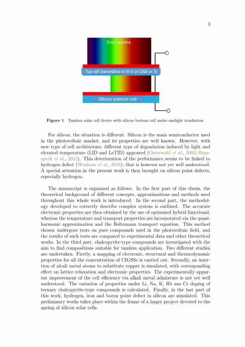
The first species represents a family of compounds which can be ternary,quaternary or penternary, depending of the composition. In this work, we are in-terested in the copper-based chalcopyrite (Coughlan et al., 2017; Abou-Ras et al.,2017), of which the most general form is CuGaxIn1−x(SySe1−y)2. These materi-als are conventionally referred to in shorthand notation, depending of the atomspresent. For exemple, CIGSSe is the general form, CIGS correspond to the qua-ternary CuIn1−xGaxS2, and CGSe to the ternary CuGaSe2. This direct band gapmaterial have high absorption properties that allows high efficiency for thin-filmsolar cells. Various properties of CIGSSe are directly linked to its compositions.A broad range of band gap, lattice parameter values and other properties can beobtained within this family of materials, especially with a new type of dopant,alkali metals. This is why its application in tandem solar cell, e.g., with silicon,is considered. In a solar cell, the absorber that captures phonons is sensible to acertain range of photon energy and thus can only absorb a part of the sunlight.In order to increase the number of photons captured, the stacking of more thanone solar cell is called a multijunction or tandem solar cell. A typical tandemstructure can be found in figure 1. The optimised efficiency for tandem solarcell have been calculated in the literature (Meillaud et al., 2006). The maximumefficiency range corresponds to a bottom cell having the band gap of around 1 eVand the top cell having the band gap of 1.5 – 1.7 eV. The objective for the studyon chalcopyrites is then to determine the composition or doping that would leadto a band gap in the desired area.
3
Figure 1 Tandem solar cell device with silicon bottom cell under sunlight irradiation.
For silicon, the situation is different. Silicon is the main semiconductor usedin the photovoltaic market, and its properties are well known. However, withnew type of cell architecture, different type of degradation induced by light andelevated temperature (LID and LeTID) appeared (Osterwald et al., 2002; Ram-speck et al., 2012). This deterioration of the performance seems to be linked tohydrogen defect (Wenham et al., 2018), that is however not yet well understood.A special attention in the present work is then brought on silicon point defects,especially hydrogen.
The manuscript is organised as follows. In the first part of this thesis, thetheoretical background of different concepts, approximations and methods usedthroughout this whole work is introduced. In the second part, the methodol-ogy developed to correctly describe complex system is outlined. The accurateelectronic properties are then obtained by the use of optimised hybrid functional,whereas the temperature and transport properties are incorporated via the quasi-harmonic approximation and the Boltzmann transport equation. This methodchosen undergoes tests on pure compounds used in the photovoltaic field, andthe results of such tests are compared to experimental data and other theoreticalworks. In the third part, chalcopyrite-type compounds are investigated with theaim to find compositions suitable for tandem application. Two different studiesare undertaken. Firstly, a mapping of electronic, structural and thermodynamicproperties for all the concentration of CIGSSe is carried out. Secondly, an inser-tion of alcali metal atoms to substitute copper is simulated, with correspondingeffect on lattice relaxation and electronic properties. The experimentally appar-ent improvement of the cell efficiency via alkali metal admixture is not yet wellunderstood. The variation of properties under Li, Na, K, Rb ans Cs doping ofternary chalcopyrite-type compounds is calculated. Finally, in the last part ofthis work, hydrogen, iron and boron point defect in silicon are simulated. Thispreliminary works takes place within the frame of a larger project devoted to theageing of silicon solar cells.

Chapter 1
Theoretical background
Before diving into their practical use, the different methods and procedures ap-plied during this thesis are described theoretically. The Hartree-Fock (HF) anddensity functional theory (DFT) are summarised before the introduction of thehybrid approach. In order to deal with the effect of temperature, the theorybehind the quasi-harmonic approximation is explained. Finally, the derivationof the electrical conductivity and other transport properties from the Boltzmanntransport equation (BTE) are demonstrated.
1.1 First-principles calculationsIn this section, the first-principles approaches are presented. They are based onthe resolution of the time-independent Schrödinger equation,
HΨ = EΨ, (1.1)
where the Hamiltonian operator H is
H = −1
2
∑
i
∇2i +
∑
i
1
2MA
∇2A −
∑
i,A
ZAriA
+∑
A,B
ZAZBRAB
+∑
i>j
1
rij, (1.2)
with i, j refering to electrons and A, B to nuclei. In order to simplify this equa-tion, the adiabatic or Born-Oppenheimer approximation (Born and Oppenheimer,1927) decouples the motion of nuclei and electrons, adopting the following formof the wavefunction:
ΨR(r) = Ψelectron(r;R)Ψnuclei(R), (1.3)
where the nuclei positions R are entering as parameters. The remaining taskis to solve the electronic part of the Schrödinger equation with the followingHamiltonian:
He = −1
2
∑
i
∇2i −
∑
i,A
ZAriA
+∑
i>j
1
rij(1.4)
= T + VeN + Vee, (1.5)
6 Chapter 1. Theoretical background
with T being the operator of the kinetic energy of the electrons, VeN the operatorof interaction between electron and nuclei and Vee the operator of interactionbetween electrons.
The later term is a sum overN independent particles difficult to evaluate. Thisequation is not exactly solvable for more than two particles. Different methodsto tackle this problem exist as we briefly explain in the following sections.
1.1.1 Hartree-Fock approximation
The first method we evoke is the Hartree-Fock (HF) approximation (Hartree,1928a,b; Fock, 1930). The objective of HF approximation is to find the wave-function of the fundamental state via a variational method. It is a purely mono-electronic model where one electron is under the influence of the mean field ofall others. In order to satisfy the Pauli’s exclusion principle, we assume thatthe many-electron wavefunction takes the form of a Slater determinant of single-electron wavefunctions (Slater, 1929):
Ψ =1√N !
ϕ1(r1) · · · ϕN(r1)...
...ϕ1(rN) · · · ϕN(rN)
. (1.6)
In this context, each electron is associated to a wavefunction ϕi and the mono-electronic Hamiltonians for the i -th electron can be written as follows:
hi = −1
2∇2i −
∑
A
ZAriA
+1
2
∑
j
[Jj(ri) + Kj(ri)
](1.7)
hi = T + VeN + J [ρ(r)] + K[ρ(r, r′)], (1.8)
where Jj the Coulombian operator between electrons and Kj the exchange oper-ator defined as
Jj(ri)ϕi(ri) =
[∫ϕ∗j(rj)
1
rijϕj(rj)
]ϕi(ri) (1.9)
andKj(ri)ϕi(ri) =
[∫ϕ∗j(rj)
1
rijϕj(ri)
]ϕi(ri). (1.10)
One of the big drawbacks of this method is that it fails to represent the correla-tion between electrons beyond the Pauli’s exclusion principle. The correlation isdefined as the difference between the real ground state energy of the system andthe one determined by HF method:
Ec = ErealTOT + EHF . (1.11)
The lack of correlation here means that an electron at a position r has no influenceon the position r′ of another electron other than Coulomb interaction. Thatleads to an overestimation of the ionic character of the system. The band gapsof semiconductors and insulators are thus highly overestimated. The J and K
1.1. First-principles calculations 7
operators lead to a calculation time proportional to N4, with N the number ofelectrons in the system. From a computational point of view, the system is either0D (molecules), 1D (chains, or polymers), 2D (surfaces) or 3D (periodic crystals).In our case, we deal with 3D cells with periodic boundary conditions.
1.1.2 Density Functional Theory
Driven by a motivation to grasp the electron correlation within a practical theory,Hohenberg and Kohn put foundation to what is nowadays known as the densityfunctional theory (DFT) (Hohenberg and Kohn, 1964). They proved that theground state energy is a functional of the electronic density and that the minimumof this functional is the true electronic density:
E0 ≤ E[ρ0] = minρ
(min
Ψ
[F [ρ] +
∫ρ(r)veN(r)d3r
]). (1.12)
In the Kohn-Sham DFT (Kohn and Sham, 1965), the wavefunction-based the-ory (WFT) is abandoned and the real density is mimicked by a density of non-interacting particles under the influence of an external potential Vxc. In thiscontext, the Hamiltonian of the mono-electronic equation is
hi = T + VeN + J [ρ(r)] + vxc(r). (1.13)
The terms are the same as for equation (1.8) except for the exchange-correlationfunctional vxc. The external potential is defined such that the electronic densityof non-interacting electrons equals the one of the real system:
ρ(r) =N∑
i=1
|ψi(r)|2. (1.14)
The only problem is that the form of the exchange-correlation functional is un-known and we need to use some approximations. The simplest is the local densityapproximation (LDA) where the exchange-correlation energy Exc is the one of anuniform electron gas:
ELDAxc =
∫εxcρ(r)d3r, (1.15)
where εxc is the exchange-correlation energy per particle of an uniform electrongas of density ρ. When density undergoes rapid spatial variations, LDA fails andthe semi-local generalised gradient approximation (GGA) is used. It takes intoaccount the density and its gradient with position ∇ρ(r). As these methods arebased on the assumption that the electron distribution is more delocalised andhomogeneous like in metal, it thus underestimates the band gap. This method iseven faster than HF as it is proportional to N3(Leach, 2001).
1.1.3 Beyond HF and DFT
Both HF and DFT suffer from drawbacks, especially their inevitable error on thedetermination of the band gap of semiconductors. Further methods called post-HF and -DFT were created to correct some of these issues. In the WFT, a many-electrons wavefunction corresponds to a particular electronic configuration where
8 Chapter 1. Theoretical background
the electrons are assigned to specific orbitals. The HF wavefunction correspondsto the ground state configuration where electrons filled the lowest orbitals. Theconfiguration interaction (CI) method (Hehre et al., 1986) takes advantage ofall these configurations. Its wavefunction is a sum of Slater determinants ofwavefunctions corresponding to specific electron configurations:
Ψ = c0Ψ0 + c1Ψ1 + c2Ψ2 + · · · . (1.16)
In this framework, the correlation is taken into account, including also the excitedstates. However, this method can be very time consuming (proportional to N12)and the full CI where all the configurations are investigated can only be done forsmall systems.
Within the DFT, the many-body GW approximation correct the electronicstructures determined by LDA or GGA. It takes advantage of Green’s functionsdescribing the photoemission process, and the screen-Coulomb interaction to ap-proximate the exact exchange self-energy (Aryasetiawan and Gunnarsson, 1998;Reining, 2018): This method thus increases the description of the electron’s in-teraction with its environment. CI and GW are not the only methods availableto reach more accurate results from HF and DFT. However, all of these methodsrequire important computational time. The time necessary for GW calculationsscales with the system size as N8. For a quick but reliable description of semi-conductors properties, hybrid functionals are a good alternative.
1.1.4 Hybrid functionals
In order to correct the drawback of DFT and HF, hybrid functionals were intro-duced by Becke (1993b). It is a pragmatic approach which combines the exactexchange of HF with DFT exchange-correlation term, since both methods giveerror of the opposite sign when compared to the experimental data. The simplestform corresponds to full-range hybrid functionals which is a linear combinationof the HF and DFT exchange:
EPBE0xc = α× EHF
x + (1− α)× EPBEx + EPBE
c , (1.17)
with α being the exchange mixing ratio. This notation should not be mixed upwith the similar labelling of the thermal expansion coefficient in the subsequentchapters. In the case of the PBE0 functional, 25% of HF exact exchange aremixed with the PBE exchange (Adamo and Barone, 1999); this exchange mixingratio is not empirical but based on a model (Perdew et al., 1996b). Because of thepotentially very demanding computational time of the exact exchange for longdistance interactions, it is decomposed into short (sr) and long (lr) range parts.This is done by splitting the Coulomb interaction as
1
r=
erfc(ωr)r
+erf(ωr)r
, (1.18)
where r is the interatomic distance between r and r′, and ω is the screeningparameter that defines the range separation. When the screening parameter is
1.2. Computational details 9
zero, equation (1.18) is equivalent to equation (1.17). One of the most used hybriddefined this way is HSE06 (Heyd et al., 2003, 2006). It is a short range hybridfunctional where the exchange energy is written as
EHSE06xc = 0.25× EHF,sr,µ
x + 0.75× EPBE,sr,µx + EPBE,lr,µ
x + EDFTc . (1.19)
In this case, the µ parameter is defined empirically. The performance of hybridfunctionals will be discussed more thoroughly in section 2.1.
1.2 Computational details
1.2.1 Basis set
In a vast majority of calculation methods in practical use, either one or theother of two families of functions serve as basis sets in order to represent thewavefunction, or the electron density.
The first family of localised basis sets is the Gaussian-type orbitals (GTO). AGaussian-type orbital (Boys, 1950), centered at some site and possessing the angu-lar symmetry Ylm(θ, φ) around it, can be expressed by equation (1.20), wherebythe parameter α gives control over the desired extension (more or less diffusecharacter) of the radial part:
gl,m(r) = B(l, α)rl exp(−αr2)Ylm(θ, φ). (1.20)
This type of basis set is easily tuned. As the product of two Gaussians is anotherGaussian, the two-center and other multicenter integrals involving these functionscan be expressed analytically and thus easy to compute. The wavefunction isexpressed as a linear combinaison of GTOs. One drawback of this type of orbitalis that, for metallic system, the number of diffuse GTOs required can be quiteimportant.
The second family is the plane-waves basis sets. A plane-wave (PW) is writtenas
p(r) =1
Ωexp(iG · r), (1.21)
with G a vector of the reciprocal lattice. The drawback here is that a largenumber of plane-wave functions is required for a good description of system withinhomogeneous electronic clouds.
Since the HF exact exchange is difficult to determine in the PW framework(Betzinger, 2007; Dziedzic et al., 2013), some codes such as VASP (Paier et al.,2005) propose an approximative way to do it but do not allow to have a self-consistent description of the system. In general, the optimisation of the geometryis done within LDA or GGA approximation. The determination of the electronicstructure is further on done at a fixed geometry with the hybrid functional. AsGTOs do not suffer from this problem, all calculations done during this thesis havebeen performed with the GTO-oriented CRYSTAL17 code (Dovesi et al., 2018). Thedescription of the basis sets used can be found in the appendix A.
10 Chapter 1. Theoretical background
1.2.2 The CRYSTAL code
CRYSTAL17 is based on the linear crystalline atomic orbital (LCAO) theory wherethe wave function is described as a sum of one-electron crystalline orbitals thatare solutions of the one-particle equation:
hiϕki = εkiϕki . (1.22)
The one-particle Hamiltonian hi is the one explicit for HF and KS in the equa-tions (1.8) and (1.13) respectively. These one-electron crystalline orbitals are inturn expressed as a sum of Bloch function φi build from local Gaussians:
ϕi(r,k) =∑
j
cij(k)φj(r,k). (1.23)
In order to computationally solve it, the one-electron Schrödinger equation canbe written in a form of matrix equation (Dovesi et al., 2005):
H(k)C(k) = S(k)C(k)E(k), (1.24)
with S(k) being the overlap matrix and C(k) the matrix of coefficients from equa-tion (1.23). In CRYSTAL, the self-consistent field (SCF) observes the followingsteps (Dovesi et al., 2005). After creating the basis sets and evaluating the over-lap matrix and the Fock matrix (corresponding to the single electron operator hi)in direct space, these matrices are then Fourier-transformed into the reciprocalspace. The Schrödinger equation is then solved at every k-point, and the Fermienergy is calculated. After that, the density matrix is determined and Fourier-transformed back into the direct space. At the end on this procedure, the totalenergy of the system is calculated. This is the cornerstone of every other calcu-lations. Once we know how to solve the Schrödinger equation for a given nucleigeometry thanks to the different theories and approximations, various proper-ties can be obtained from different types of calculations. Below, we outline thequasi-harmonic approximation and the transport properties calculations as twoimportant parts of this work.
1.3 Quasi-harmonic approximationGeometry optimisations, once performed, lead to the equilibrium position in thepotential energy surface where the other types of calculations can take place.However in a real crystal, the lattice is not rigid and each atom moves aroundits equilibrium position. The effect of temperature on the crystal vibrationalproperties can be taken into account via the crystal vibrational properties. Whenlooking for small variations around the equilibrium position, the Taylor expansion,see -equation (1.25), comes in handy:
f(x) = f(x0) + (x− x0) · df(x0)
dx+
(x− x0)2
2· df
2(x0)
d2x+ · · · (1.25)
By definition, the first derivative of energy over displacements at the equilibriumposition is zero so that the first assumption is to consider only the quadratic
1.3. Quasi-harmonic approximation 11
term. This would correspond to the harmonic approximation for atomic vibra-tions. The Hessian or dynamic matrix is obtained by the finite displacement tech-nique, whereby the atoms are shifted one by one from their equilibrium positions.The dynamical equations which contain the Hessian are then diagonalised, yield-ing the phonon eigenvalues (frequencies squared) and eigenvectors (displacementpatterns within each mode). By default in CRYSTAL, the phonon calculationis done at the Γ point. In order to take phonons with other (commensurate)wavevectors into account, one can resort to constructing a supercell which wouldaccommodate the vibration wave in question. The phonon calculation is e.g.,useful for checking the dynamical stability of presumably equilibrium structure.An instability could be identified by detecting an imaginary phonon frequency,that means that a combined displacement pattern exists which would lower thetotal energy on displacement from the equilibrium. Once the phonon frequenciesare calculated in the harmonic approximation, the energy levels of correspondingquantum oscillators can be artificially populated with Bose-Einstein distributionfor a specific temperature. Even as this would allow the calculation of differentthermodynamic properties, a major drawback of such approach is that it doesnot provide a mechanism that would relate the variation of interatomic distanceswith temperature. That means for example that there is no thermic expansionof the crystal or that the thermal conductivity will be infinite.
This problem can be tackled down via the incorporation of inharmonic termsbut this requires to solve more complex equation. A simpler solution is the quasi-harmonic approximation (QHA) that keeps the harmonic expression but adds anexplicit dependence of vibration phonon frequencies on volume.
The quasi-harmonic approximation has been implemented in CRYSTAL17 (Erba,2014). An automated algorithm computes the influence of the temperature andpressure on different structural and thermodynamic properties. The procedureneeds to start from an optimised geometry at 0 K, either from a previous workor done at the beginning of the calculation. Depending of the chosen param-eters, the algorithm performes structural optimisation and phonon calculationfor different contracted or expanded systems around the zero-temperature equi-librium position. Once all those structures have been computed, their volumeand energy can be used to fit the purely electronic internal energy as a functionof volume via different equations-of-state (EOS) from the literature. CRYSTALproposes different EOS but uses the third-order Birch-Murnaghan (Birch, 1947;Murnaghan, 1944) for further thermodynamic calculations. Volume dependenceof each phonon frequency is then individually fitted with second or third-orderpolynomes.For a given temperature, the Helmholtz free energy is calculated thanks to thefollowing equations :
FQHA(T, V ) = U0(V ) + FQHAvib (T, V ), (1.26)
FQHAvib (T, V ) =EZP
0 (V ) + kBT∑
kp
[ln
(1− e−
~ωkp(V )
kBT
)](1.27)

12 Chapter 1. Theoretical background
andEZP
0 (V ) =∑
kp
~ωkp(V )/2. (1.28)
For each temperature, the Helmholtz free energy is minimised in order to ob-tain the equilibrium structure. In that way, the temperature dependence of thevolume can be plotted. As several properties depend on the derivative of thevolume’s variation with the temperature, the number of temperature steps mustbe sufficiently large.
Once the geometry has been fitted at each temperature, the band gap can becalculated for this fixed geometry.
1.4 Electrical transport properties
1.4.1 Boltzmann transport equation
In order to study the classical transport of charge carrier in the bulk, the Boltz-mann transport equation (BTE) is used that deals with the local concentrationof carriers in the state k close to the point r and describes how this concentrationchanges in time (Allen, 1996). Even though the transport properties need, inprinciple, to be calculated by taking into account the phonon contribution, onlythe electronic contribution will be considered in this thesis. Three different effectsshould be indicated in what concerns the charge carriers’ distribution.
• The first one is their diffusion. If the velocity of a carrier in state k isdenoted vk, the carrier will travel a distance tvk in an interval t, with thevelocity:
vα (i,k) =1
~∂εi,k∂kα
. (1.29)
Thanks to Liouville’s theorem, which states that "the phase-space distribu-tion function is constant along the trajectories of the system", we can writefor the probability density function f :
fk(r, t) = fk(r− tvk, 0), (1.30)
so that : [∂fk∂t
]
diff
= −vk∂fk∂r
= −vk∇rfk. (1.31)
• The second effect concerns constant external fields that change the vectork at a rate of
dkdt
=e
~
(E +
1
cvk ∧H
). (1.32)
This corresponds to the velocity in k-space so that by analogy with equa-tion (1.30), the impact of the field is
[∂fk∂t
]
field
= − e~
(E +
1
cvk ∧H
)∇kfk. (1.33)

1.4. Electrical transport properties 13
• The last one is the scattering effect. It is more complicated to express andwe generally stay in the scope of elastic scattering.
The BTE states that the net rate of change of fk(r) with time is zero :[∂fk∂t
]
diff
+
[∂fk∂t
]
field
+
[∂fk∂t
]
scatt.
= 0. (1.34)
The distribution function can be seen as the perturbation, gk(r), of the equilib-rium Fermi-Dirac distribution function defined at spatially variable temperatureT (r):
fk(T (r)) = f 0k(T (r)) + gk(r), (1.35)
with:f 0k =
1
eεk−µkBT + 1
. (1.36)
In the absence of temperature gradients (∇rfk = 0) and for an external forceconsisting only of a low electric field E (H = 0), the equation (1.34) becomes:
(∂fk(T )
∂t
)
s
= eEvk
(−∂f
0k(T )
∂ε
). (1.37)
1.4.2 Relaxation Time approximation
In order to solve the BTE, the scattering effect term must be explicated. However,instead of defining every possible scattering effects, the following assumption ismade: [
∂fk∂t
]
scatt.
= −1
τ· gk, (1.38)
with τ the relaxation time needed for a system without the influence of externalfields to go back to its equilibrium. This can also be seen as
gk(t) = gk(0)e−tτ . (1.39)
By replacing equation (1.38) in equation (1.37), we obtain
gk = −τvk · eE(−∂f
0k(T )
∂ε
). (1.40)
Even though the relaxation time depends on the band index and the vector di-rection, it is usually taken as a constant in the constant relaxation time approxi-mation (CRTA).
1.4.3 Electrical conductivity
The number of carriers in the volume dk is g(k)dk4π3 so that we can write the current
density in the band n as
Jn = −e∫
1
4π3vn,kgn,kdk. (1.41)
14 Chapter 1. Theoretical background
As the electrical conductivity is the sum of the contribution of each band Jn =σnEn,
σ =∑
n
e2
∫1
4π3τnvn,kvn,k
(−∂f
0k(T )
∂ε
)dk, (1.42)
and the inverse mass tensor,
M−1βu (i,k) =
1
~2
∂2εi,k∂kβ∂ku
, (1.43)
the different transport properties can be written :
[σ]i,j (T ;µ) = e2
∫Σi,j (ε)
[−∂f(µ,E, T )
∂E
]dE, (1.44)
[σS]ij =e
T
∫Σi,j (ε)
[−∂f(µ,E, T )
∂E
](E − µ)dE, (1.45)
and[κe]i,j (T ;µ) =
1
T
∫Σi,j (ε)
[−∂f(µ,E, T )
∂E
](E − µ)2dE, (1.46)
with the transport distribution function defined as
Σij(E) =1
V
∑
n,k
vi(n, k)vj(n, k)τn,kδ(E − En,k). (1.47)
1.4.4 Computational approaches
During the last decade, different codes were developed in order to calculate thetransport properties from the BTE. The underlying theory is usually the same.
First, the rigid band approximation (RBA) implies that the band structuredoes not change under the influence of temperature or chemical potential.
The different packages principally differ in their way to interpolate the bandstructure. One of the most famous package is BoltzTraP (Madsen and Singh,2006) that uses a Fourier expansion to interpolate the band. This numericalinterpolation offers the advantage of directly obtaining the group velocity andthe inverse mass tensor from the derivative with the finite-difference procedure.The problem with this method is the potential band crossing at the boundaries. Inthis case, a very fine k-grid needs to be used to correctly describe the phenomena.To avoid that, Scheidemantel et al. (2003) calculated the group velocities withthe momentum matrix , also called the intraband optical matrix element:
vn,k =1
mpn,k =
1
m〈Ψn,k|p|Ψn,k〉 . (1.48)
The new version of BoltzTraP, simply called BoltzTraP2 (Madsen et al., 2018),had implemented the momentum matrix approach. Another method consists inusing Wannier functions as in BoltzWann (Pizzi et al., 2014). This analyticalmethod uses the localised Wannier functions on a coarse k-point grid to avoid
1.5. Summary and conclusion 15
the finite-difference methods. Boltzmann transport equation has also been im-plemented in CRYSTAL17 within the RBA and RTA.
Until now, all the codes cited performed calculations under the constant re-laxation time approximation (CRTA). However, this is not a necessary limitation.For example, one can abandon the CRTA by varying the relaxation time withthe energy. Another possible way is to take into account different types of scat-tering process. This is the case for the work of Faghaninia (Faghaninia et al.,2015; Faghaninia, 2016) who suggested an abinitio model for calculating mobilityand Seebeck coefficient using the Boltzmann transport (aMoBT) which was imple-mented in the AMSET (Faghaninia et al., 2015, 2017) script. This Python moduleapproximates scattering effects via different properties such as the phonon fre-quencies and the dielectric constant. The acoustic deformation potential, ionisedimpurity, piezoelectric and polar optical phonon differential scattering rates areavailable in this code.
In this thesis, we tested BoltzTraP2 and CRYSTAL17 . As we used CRYSTAL17for all the type of calculation, we first calculated the transport properties ofthe build-in module of CRYSTAL17 . The calculation works smoothly for thematerial tested in a within a bearable time. A defective system of 32 atoms withlow symmetry takes less than three hours. However, the important number ofintegrals to calculate and store during the time of simulation results in creatingfiles of several gigabytes of data. For one simulation, 1.2 Tb of temporary datahave been accumulated. This is problematic because of the limit of memory of thecomputer. Even if the jobs are launched sequentially, one heavy file can stop theprogram due to a memory error. This is why we turned to the second solution,the python module BoltzTraP2. It is not configured for CRYSTAL17 output butwe created the necessary interface. BoltzTraP2 can be used in command line oras a python library. Here, only the command line function was used.
1.5 Summary and conclusionAll these methods are complementary and can be used to reach different types ofproperties. The hybrid functionals are a pragmatic way to correct the band gapproblem of Hartree-Fock and density functional theory and prevent the compu-tational cost of more sophisticated methods. Quasi-harmonic approximation andBoltzmann transport equation enable us to access the temperature dependenceof various properties and the transport properties of our material. We explainedthe underlying theory in this chapter and their practical use and optimisation willbe developed in the next one. The properties calculated from the quasi-harmonicapproximation and the transport properties will be compared to experimentaldata and the performance of different functionals.

Chapter 2
Hybrid functional performances
The main objective of this thesis is to access macroscopic properties of defectivematerials in the context of photovoltaic applications. In this thesis, hybrid func-tionals have been optimised to reproduce the experimental value of the studiedmaterials’ band gap. This method will first be explained before comparing theoptimised hybrid functionals to the theoretical and experimental works of litera-ture for perfect compounds in order to verify the reliability of this method. Oncethese are obtained, the temperature effect will be tested via the quasi-harmonicapproximation. Finally, the Boltzmann transport equation will be solved for thedetermination of macroscopic transport properties. The methodology introducedin this chapter is tested for pure compounds and its results are compared withthe experimental and computational works from literature.
2.1 Hybrid functionals
2.1.1 Hamiltonian optimisation
State-of-the-art
As we saw in section 1.1.4, hybrid functionals were created to correct the “bandgap problem” of density functional theory and Hartree-Fock approximation. Theycould be an interesting alternative to accurate but time-consuming methods suchas GW. In the full-range hybrid functionals, a percentage of the HF exact ex-change, called α, see equation (1.17), is incorporated into the DFT functionals.Other parameters such as the screening parameter are used in short- and long-range hybrid functionals but we limit ourselves to the full-range hybrid function-als in this thesis. In the early years of hybrid functionals, different Hamiltonianswere created with a fixed value of the exchange mixing ratio. For example, PBE0(Adamo and Barone, 1999) uses a PBE functional (Perdew et al., 1996a) with 25%of exact exchange from HF. This value was obtained without any experimentalconsiderations (Perdew et al., 1996b). Nevertheless, PBE0 is known to overesti-mate the band gap of low band gap materials and underestimate the one of highband gap materials (Alkauskas et al., 2011). It is more a compromise than anabsolute and perfect value. Since the middle of the 2000s, discussions about theoptimised amount of exact exchange to incorporate in DFT functionals have been

18 Chapter 2. Hybrid functional performances
set. This value can be system-dependent but its determination must be done inpreliminary calculation. Alkauskas et al. (2008) tuned the exchange mixing ratioto reproduce the experimental band gap for the determination of band offsetsat silicon-based semiconductors interface. They found that the lineup of bulkreference levels is practically independent of α. In the same year, the same groupobserved a linear impact of α on the evolution of the valence- and conduction-band edges of Si and Ge (Broqvist et al., 2008). In both cases, the DFT functionalchosen was PBE and the optimised values of α were 0.11, 0.15 and 0.15 for Si,Ge and SiC respectively. Moreover, they observed that the optimised value ofthe exchange mixing is related to an effective static screening of the long-rangeinteraction (Alkauskas et al., 2008). The link between the optimised value andthe high frequency dielectric constant (ε∞) has also been found by Shimazaki andAsai (2008) at the same period. The relation is
α ' 1
ε∞. (2.1)
This can be explained by observing the similarity with GW approximation (Alka-uskas and Pasquarello, 2011). The non-local exchange-correlation potential of hy-brid functionals can be seen as the many-electron exchange-correlation self-energyin the GW approximation. In this approximation, the long-range interaction canbe compared to a screened exchange whose asymptotic is the inverse of the dielec-tric constant times the distance between r and r′. As the DFT, semi-local, termsof the hybrid functional are short-ranged, the long-range interactions are fully cov-ered by the non-local, HF exact exchange α/|r− r′|. Since the cited observationof Alkauskas and Pasquarello, numerous works used the inverse of the dielectricconstant as an approximation for the exchange mixing ratio (Alkauskas et al.,2011; Marques et al., 2011; Conesa, 2012; Hinuma et al., 2017; Shimazaki andNakajima, 2014; Fritsch et al., 2017). In order to automatise the process, someself-consistent methods have been proposed (Shimazaki and Asai, 2009; Skoneet al., 2014). They suggest to calculate the dielectric constant self-consistentlyuntil convergence by changing at each iteration the value of alpha. The methodproposed by Skone et al. (2014) was implemented in CRYSTAL17 (Erba, 2017).The procedure is exposed in figure 2.1. In this algorithm, the dielectric constantis calculated via a coupled-perturbed Kohn-Sham or HF (CPKS or CPHF) cal-culation (Ferrero et al., 2008) at each iteration for a given value α defined as inequation (2.1).
Band gap optimised hybrid functional
For tandem applications, the band gaps of the two absorbers need to be comple-mentary to capture as much of the incident light as possible. In order to have aqualitative and quantitative description of the electronic properties such as theband structure, we adjusted α in order to define a hybrid functional that leads toa band gap which matches its experimental value for each material. A fully au-tomated algorithm for the determination of the optimal fraction was developed.
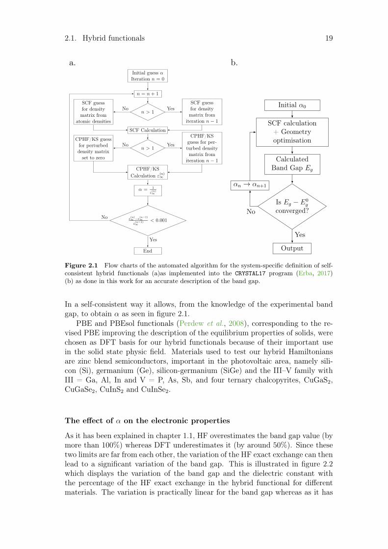
2.1. Hybrid functionals 19
a. b.Initial guess αIteration n = 0
n = n + 1
SCF guessfor densitymatrix from
atomic densities
n > 1
SCF guessfor densitymatrix from
iteration n − 1
SCF Calculation
CPHF/KS guessfor perturbeddensity matrixset to zero
n > 1
CPHF/KSguess for per-turbed densitymatrix from
iteration n − 1
CPHF/KSCalculation ε(n)
∞
α = 1
ε(n)∞
ε(n)∞ −ε(n−1)
∞ε(n−1)∞
< 0.001
End
No Yes
No Yes
No
Yes
Initial α0
SCF calculation+ Geometryoptimisation
CalculatedBand Gap Eg
Is Eg − E0g
converged?
Output
αn → αn+1
No
Yes
Figure 2.1 Flow charts of the automated algorithm for the system-specific definition of self-consistent hybrid functionals (a)as implemented into the CRYSTAL17 program (Erba, 2017)(b) as done in this work for an accurate description of the band gap.
In a self-consistent way it allows, from the knowledge of the experimental bandgap, to obtain α as seen in figure 2.1.
PBE and PBEsol functionals (Perdew et al., 2008), corresponding to the re-vised PBE improving the description of the equilibrium properties of solids, werechosen as DFT basis for our hybrid functionals because of their important usein the solid state physic field. Materials used to test our hybrid Hamiltoniansare zinc blend semiconductors, important in the photovoltaic area, namely sili-con (Si), germanium (Ge), silicon-germanium (SiGe) and the III–V family withIII = Ga, Al, In and V = P, As, Sb, and four ternary chalcopyrites, CuGaS2,CuGaSe2, CuInS2 and CuInSe2.
The effect of α on the electronic properties
As it has been explained in chapter 1.1, HF overestimates the band gap value (bymore than 100%) whereas DFT underestimates it (by around 50%). Since thesetwo limits are far from each other, the variation of the HF exact exchange can thenlead to a significant variation of the band gap. This is illustrated in figure 2.2which displays the variation of the band gap and the dielectric constant withthe percentage of the HF exact exchange in the hybrid functional for differentmaterials. The variation is practically linear for the band gap whereas as it has
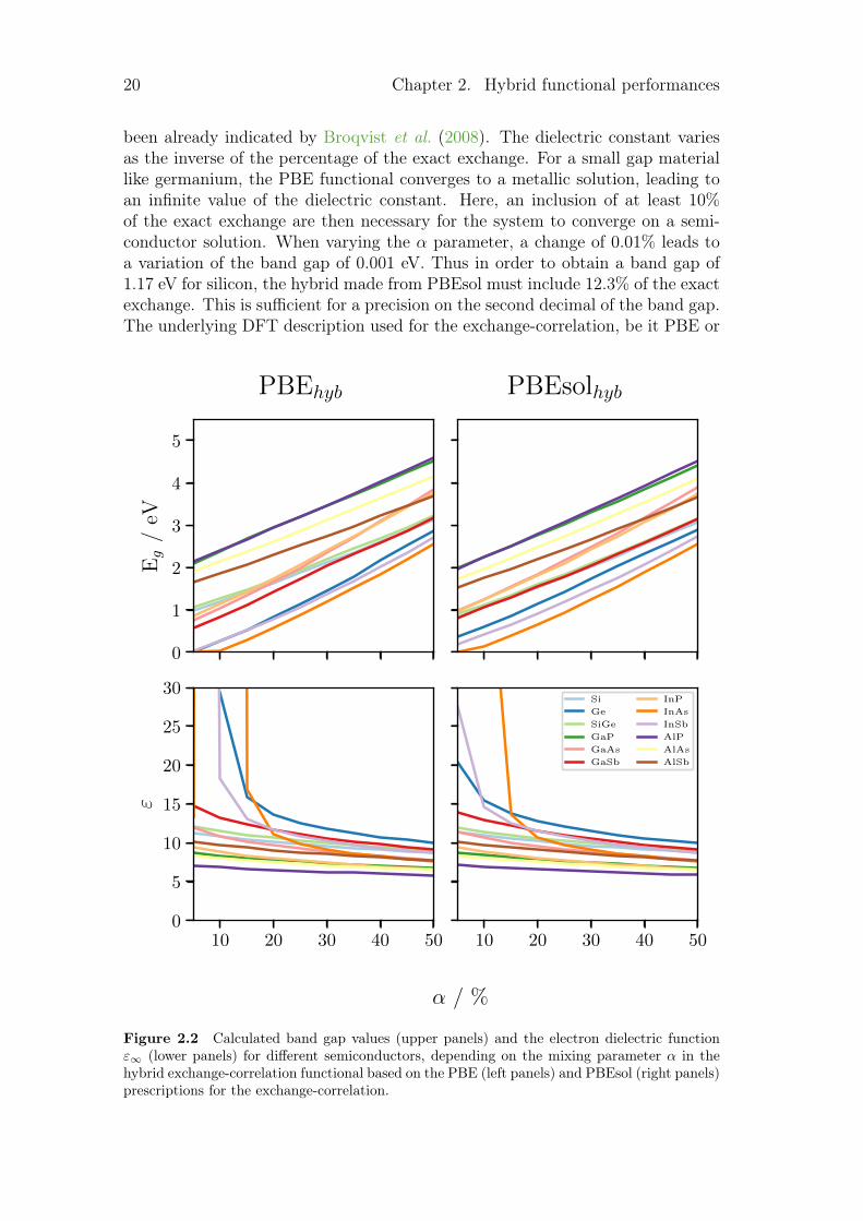
20 Chapter 2. Hybrid functional performances
been already indicated by Broqvist et al. (2008). The dielectric constant variesas the inverse of the percentage of the exact exchange. For a small gap materiallike germanium, the PBE functional converges to a metallic solution, leading toan infinite value of the dielectric constant. Here, an inclusion of at least 10%of the exact exchange are then necessary for the system to converge on a semi-conductor solution. When varying the α parameter, a change of 0.01% leads toa variation of the band gap of 0.001 eV. Thus in order to obtain a band gap of1.17 eV for silicon, the hybrid made from PBEsol must include 12.3% of the exactexchange. This is sufficient for a precision on the second decimal of the band gap.The underlying DFT description used for the exchange-correlation, be it PBE or
0
1
2
3
4
5
Eg
/eV
PBEhyb PBEsolhyb
10 20 30 40 500
5
10
15
20
25
30
ε
α / %
10 20 30 40 50
Si
Ge
SiGe
GaP
GaAs
GaSb
InP
InAs
InSb
AlP
AlAs
AlSb
Figure 2.2 Calculated band gap values (upper panels) and the electron dielectric functionε∞ (lower panels) for different semiconductors, depending on the mixing parameter α in thehybrid exchange-correlation functional based on the PBE (left panels) and PBEsol (right panels)prescriptions for the exchange-correlation.

2.1. Hybrid functionals 21
10 20 30 40 50
α / %
5.4
5.6
5.8
6.0
6.2
a/
APBEhyb
10 20 30 40 50
α / %
PBEsolhybsi
ge
sige
gap
gaas
gasb
inp
inas
insb
alp
alas
alsb
Figure 2.3 Influence of the percentage of exact exchange in the hybrid functional on thestructural parameters for different materials.
PBEsol, hardly makes a noticeable difference. Moreover, as their impact on thefinal result decreases with the increase of α, they tend to the same HF limit.
Impact on the structural properties
Even though we are interested here in the correct description of the band gap,the other parameters are of significant importance. The structural propertieshave also a key role for tandem application where the lattice parameters of thetwo compounds must be similar to avoid lattice mismatch and thus growth andadhesion problems. According to literature, α does not have a strong influence onthe structural properties (Deák et al., 2005; Paier et al., 2006; Heyd et al., 2005).Figure 2.3 shows the variation of the lattice parameter a for Si, Ge, SiGe, GaP,GaAs and GaSb. Similar to the behaviour of the band gap, the lattice parametercan be seen at first approximation as linear with the percent α. However, unlikethe variation of the band gap, the lattice parameter decreases for higher α. Therelative variation of each one is of the order of magnitude of 0.1 for the wholerange of percentage of exact exchange studied.
If we turn this differently, in an attempt to optimise our hybrid not accordingto the band gap but to the lattice parameter, the percentage would need tobe changed drastically for a very small change of the lattice parameter. Thus,the corresponding value of the band gap might happen to be too far from theexperimental value.
Optimised HF exact exchange percentage
Figure 2.4 shows the values of the mixing parameter α, optimised by the pro-cedure described in figure 2.1, and grouped as function of calculated band gap
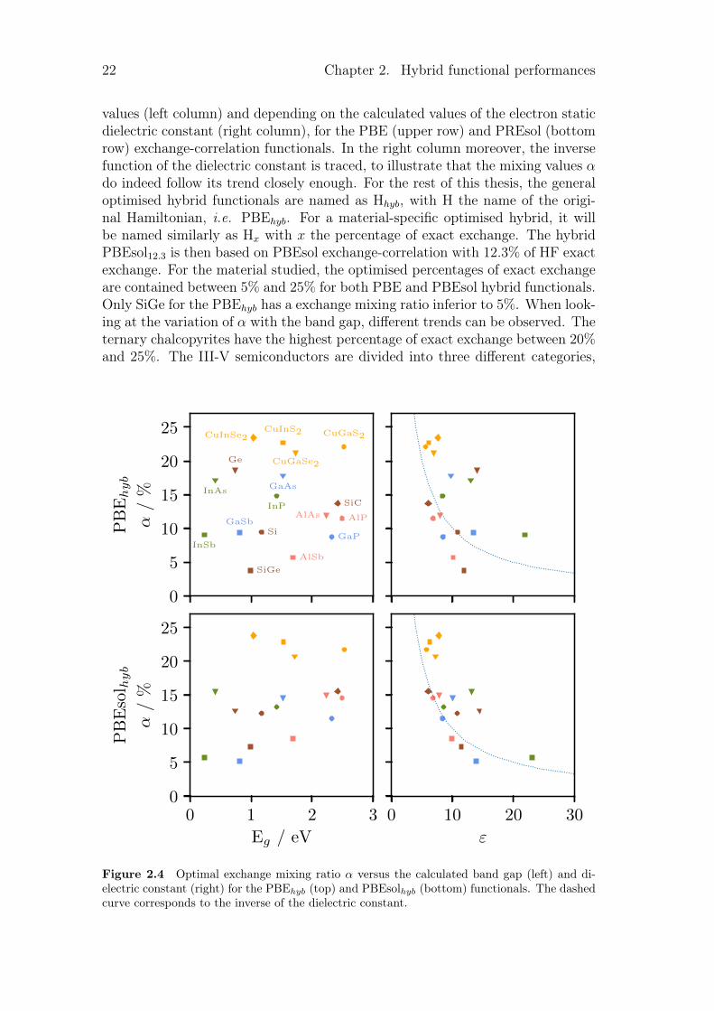
22 Chapter 2. Hybrid functional performances
values (left column) and depending on the calculated values of the electron staticdielectric constant (right column), for the PBE (upper row) and PREsol (bottomrow) exchange-correlation functionals. In the right column moreover, the inversefunction of the dielectric constant is traced, to illustrate that the mixing values αdo indeed follow its trend closely enough. For the rest of this thesis, the generaloptimised hybrid functionals are named as Hhyb, with H the name of the origi-nal Hamiltonian, i.e. PBEhyb. For a material-specific optimised hybrid, it willbe named similarly as Hx with x the percentage of exact exchange. The hybridPBEsol12.3 is then based on PBEsol exchange-correlation with 12.3% of HF exactexchange. For the material studied, the optimised percentages of exact exchangeare contained between 5% and 25% for both PBE and PBEsol hybrid functionals.Only SiGe for the PBEhyb has a exchange mixing ratio inferior to 5%. When look-ing at the variation of α with the band gap, different trends can be observed. Theternary chalcopyrites have the highest percentage of exact exchange between 20%and 25%. The III-V semiconductors are divided into three different categories,
0
5
10
15
20
25
α/
%
Si
Ge
SiGe
SiC
GaP
GaAs
GaSb
InP
InAs
InSb
AlPAlAs
AlSb
CuGaS2
CuGaSe2
CuInS2CuInSe2
PB
Ehyb
0 1 2 3
Eg / eV
0
5
10
15
20
25
α/
%
PB
Eso
l hyb
0 10 20 30
ε
Figure 2.4 Optimal exchange mixing ratio α versus the calculated band gap (left) and di-electric constant (right) for the PBEhyb (top) and PBEsolhyb (bottom) functionals. The dashedcurve corresponds to the inverse of the dielectric constant.
2.1. Hybrid functionals 23
for which the value of α is dictated by the V’s atoms. Phosphide-based materialsare in the same range of percentage, just as arsenide-based and antimonide-basedmaterials. This is true for both PBE and PBEsol hybrid functionals. SiGe is notin the middle of a line between Si and Ge even though its band gap is comprisedbetween their values. In general, two materials with the same approximate bandgap do not have the same optimised α. AlSb and CuGaSe2 each have a band gaparound 1.70 eV but their optimised exchange mixing ratio differs from more than10% for PBEsol-based and more than 15% for PBE-based hybrid functional. Onthe contrary, different materials with various band gap may have practically thesame optimised exchange mixing ratio. This is the case for InSb, GaSb, Si andGaP for a PBEhyb optimised with 10% of exact exchange for band gaps going from0.23 eV to 2.32 eV. Thus, there is no direct correlation between the optimisedamount of exact exchange to incorporate into DFT functionals and the band gapof the material. Other parameters like the chemical nature of the compoundmight have an influence.
For the dielectric, our results are in accordance with equation (2.1). Theglobal description of α by the inverse dielectric constant is well reproduced forPBEsol functional and to a lesser extent for PBE where there is more dispersion.However, even though the description of α by the inverse dielectric constant canbe a first good approximation, some difference arise. As for the band gap, twomaterials with the same dielectric constant do not have the same optimised α.This is true for both PBE and PBEsol-based hybrids.
Comparison with the performance of the hybrid functionals optimisedusing Skone’s method
Here, we will compare our Hamiltonians with functionals optimised with Skone’smethod that have been implemented in CRYSTAL17. Table 2.1 shows the per-formance of the two types of hybrid functionals on the structural, dielectric andelectronic properties. The first column for each material corresponds to the per-centage of exact exchange incorporated in the functional. The values of α aresensitively different for both methods in numerous cases. In Ge, for example,when our hybrids have α equal to 19 % and 13 % for PBEhyb and PBEsolhyb,the dielectric dependent functionals have 6 % and 4 % respectively. This leadsto different calculated values for the band gap. For PBE and PBEsol-based di-electric dependent hybrid Hamiltonian, the band gap is underestimated. PBEε∞even gives a nearly disappearing band gap (0.04 eV). The same test was madefor the ternary compound and PBEsolε∞ converged, for CuInSe2, to a solutionwith closing band gap. The hybrid functionals optimised taking into account thecalculated values of the dielectric constant are not well suited for an accurate de-scription of the band gap. The description of the dielectric constant is not bettercompared to the one obtained with PBEhyb and PBEsolhyb. The performances areglobally the same, except for the band gap. Hence, our hybrids are more adaptedfor photovoltaic applications where the electronic properties are of most interest.

24 Chapter 2. Hybrid functional performances
Table 2.1 Comparison of the performance of two type of self-consistent hybrid Hamiltoniansin reproducing the various properties of semiconductors.
Si Ge SiGeα a ε Eg α a ε Eg α a ε Eg
PBEEg 9.45 5.464 10.85 1.17 18.57 5.684 14.06 0.74 3.79 5.542 11.87 0.99
PBEsolEg 12.29 5.432 10.78 1.17 12.62 5.625 14.40 0.74 7.37 5.485 11.43 0.99
PBEε∞ 9.1848 5.465 10.88 1.16 5.86 5.717 17.05 0.04 8.52 5.517 11.73 1.13
PBEsolε∞ 9.0464 5.434 11.05 1.02 3.69 5.637 27.07 0.30 8.61 5.463 11.60 0.99
Others 5.46 11.76 0.99 15.65 0.71
Exp. 5.430 11.4 1.17 5.652 15.36 0.74 5.537 13.95 0.99
GaP GaAs GaSbα a ε Eg α a ε Eg α a ε Eg
PBEEg 8.75 5.474 8.45 2.32 17.75 5.663 9.79 1.52 9.37 6.111 13.43 0.81
PBEsolEg 11.53 5.418 8.35 2.32 14.58 5.606 9.99 1.52 5.16 6.045 13.87 0.81
PBEε∞ 12.06 5.469 8.29 2.51 8.78 5.686 11.38 0.94 6.91 6.107 14.47 0.78
PBEsolε∞ 11.99 5.418 8.34 2.34 9.23 5.613 10.83 1.18 7.37 6.032 13.57 0.97
OthersExp. 5.447 8.46 2.31 5.648 10.58 1.52 6.096 13.80 0.81
InP InAs InSbα a ε Eg α a ε Eg α a ε Eg
PBEEg 14.81 5.931 8.38 1.42 17.08 6.110 13.01 0.41 9.05 6.516 21.89 0.23
PBEsolEg 13.23 5.877 8.55 1.42 15.47 6.047 13.15 0.41 5.73 6.445 22.99 0.23
PBEε∞ 11.26 5.940 8.88 1.21
PBEsolε∞ 11.36 5.880 8.80 1.32
OthersExp. 5.866 9.56 1.42 6.058 11.78 0.41 6.479 16.76 0.23
AlP AlAs AlSbα a ε Eg α a ε Eg α a ε Eg
PBEEg 11.50 5.497 6.81 2.49 11.96 5.687 7.90 2.23 5.70 6.149 10.11 1.69
PBEsolEg 14.57 5.463 6.80 2.49 15.02 5.643 7.77 2.23 8.53 6.093 9.89 1.69
PBEε∞ 14.90 5.491 6.71 2.67 12.62 5.689 7.92 2.26 10.20 6.151 9.80 1.88
PBEsolε∞ 14.71 5.463 6.79 2.50 12.61 5.647 7.93 2.10 10.21 6.102 9.79 1.77
Others 7.23 2.37
Exp. 5.464 9.8 2.50 5.660 8.2 2.23 6.136 9.88 1.69
Table 2.2 Calculated mean absolute relative error (MARE) in percent for each tested Hamil-tonians for the structural properties (a), the bulk modulus (B), the band gap (Eg), the dielectricconstant (ε), the Gamma phonon frequencies (ω), the average of all the properties (MAREtot)and all except the band gap (MARE0)).
Hamiltonian a B Eg ε ω MAREtot MARE0
HF 1.05 36.95 350.80 34.76 10.92 86.90 20.92
PBE 0.52 12.09 43.00 30.6 0.39 17.32 10.90
PBE0 1.34 22.46 31.49 11.23 5.89 14.48 10.23
PBEsol 0.14 20.30 19.69 40.56 2.59 16.66 15.90
PBEsol0 0.64 33.02 52.45 15.98 7.56 21.93 14.30
LDA 0.47 18.77 41.01 14.96 4.22 15.89 9.61
B3LYP 1.22 14.36 8.19 34.30 1.37 11.89 12.81
HSE06 1.29 21.20 18.14 5.18 11.45 9.22
HSEsol 0.56 31.49 20.85 6.95 14.96 13.00
M06 1.10 18.95 18.20 3.26 10.38 7.77
M06L 1.07 16.21 55.48 1.20 18.49 6.16
HISS 1.65 28.50 29.46 8.68 17.07 12.94
PBEhyb 0.45 20.24 2.15 3.80 3.11 5.95 6.90
PBEsolhyb 0.40 27.47 0.26 3.69 5.29 7.42 9.21
2.1. Hybrid functionals 25
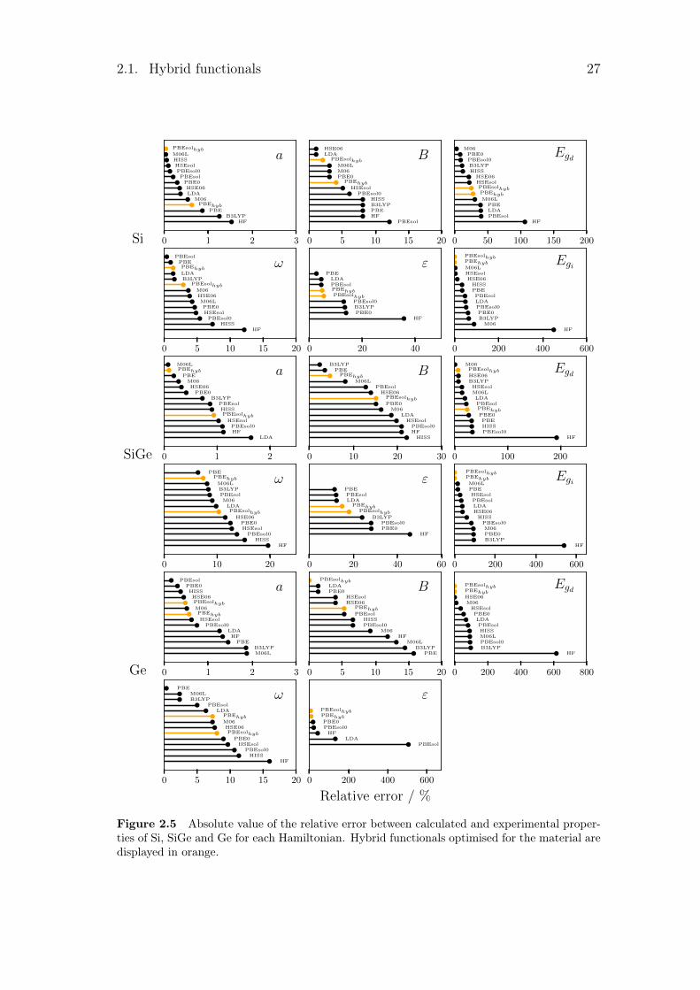
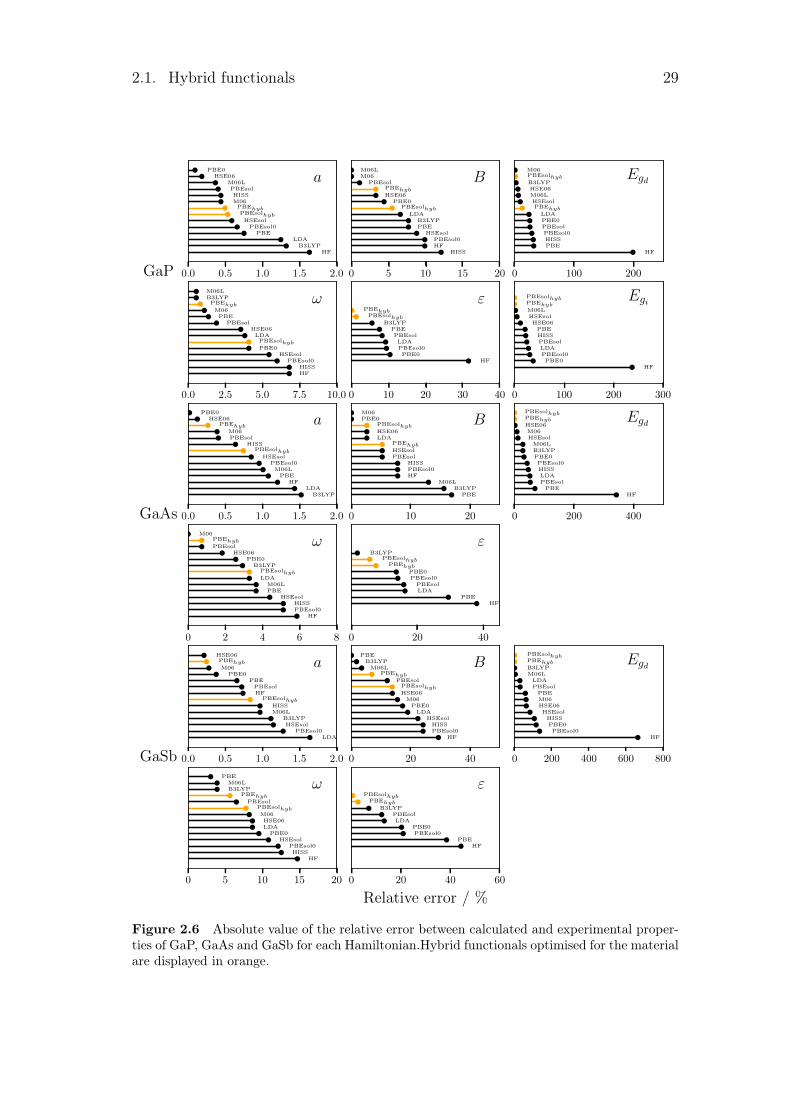
2.1.2 Hamiltonian benchmark
Method
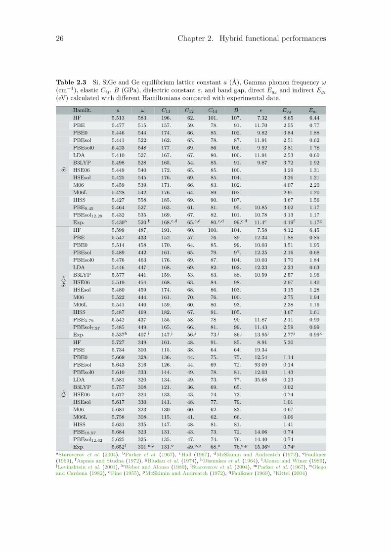
Once the hybrid functionals were optimised to accurately describe the exper-imental band gap, we tested and compared them against the other Hamilto-nians from literature. Several exchange-correlation functionals were used forthe comparison. The local density approximation (LDA) is represented by aDirac-Slater exchange (Dirac, 1930) plus a Vosko-Wilk-Nusair correlation po-tential (Vosko et al., 1980). The varieties of the GGA used were the Perdew-Burke-Ernzerhof (PBE) exchange-correlation functional (Perdew et al., 1996a),and PBEsol (Perdew et al., 2008). Different hybrid HF/KS functionals were alsoconsidered: three global, B3LYP (Becke, 1993a; Lee et al., 1988), PBE0 (Adamoand Barone, 1999) and PBEsol0, three range-separated, HSE06 (Heyd et al., 2003,2006), HSEsol (Schimka et al., 2011; Perdew et al., 2008) and HISS (Hendersonet al., 2007, 2008), and two meta-GGA, M06 (Zhao and Truhlar, 2006) and M06L(Zhao and Truhlar, 2008). All those Hamiltonian were tested by comparing theirequilibrium geometry a (Å), Gamma phonon frequency ω (cm−1), elastic Cij andB (GPa) as well as the dielectric properties ε∞ and direct and indirect band gapEgd,i (eV), with experimental data. The dielectric properties are calculated viathe coupled-perturbed HF/KS which option, however, is not yet implemented forHSE06, HSEsol, M06, M06L and HISS. The tables 2.3 to 2.8 regroup the differentcalculated values for each material and the corresponding relative error with theexperimental data are shown in the figures 2.5 to 2.11.
Results
Several patterns can be pointed out in the different tables. The first one is thedirect or indirect behaviour of the band gap. For GaP, GaSb and AlAs, the calcu-lated band gaps converge to the wrong solution for functionals such as B3LYP orM06. For the second one, as LDA and GGA underestimate the band gap, smallband gap semiconductors are sometimes seen as metal by some LDA or GGA.This is the case here for Ge, InaS, InSb and CuInSe2 which become metallic forseveral Hamiltonians. Finally, some calculated band gaps are really close to zero.This leads to an infinite dielectric constant, as for InSb with the PBEsol func-tional with its 0.01 eV. All these problems are linked to the electrical properties.With the optimised hybrid functionals, those types of problems disappear.
Relative error from experimental data
In order to have a general point of view of the different error with experimentaldata, these errors are quantified in table 2.2. In this table, the mean absolute rel-ative error (MARE) was calculated for each family of properties. The mean valueregrouping the different lattice parameters a, c and u can be found in the firstcolumn, noted a. For every functional, it has been obtained by taking the averagevalue of the mean absolute relative value for all the material. For the structuralproperties, different constants are calculated. We then took the average value of
26 Chapter 2. Hybrid functional performances
Table 2.3 Si, SiGe and Ge equilibrium lattice constant a (Å), Gamma phonon frequency ω(cm−1), elastic Cij , B (GPa), dielectric constant ε, and band gap, direct Egd and indirect Egi
(eV) calculated with different Hamiltonians compared with experimental data.
Hamilt. a ω C11 C12 C44 B ε Egd EgiHF 5.513 583. 196. 62. 101. 107. 7.32 8.65 6.44
PBE 5.477 515. 157. 59. 78. 91. 11.70 2.55 0.77
PBE0 5.446 544. 174. 66. 85. 102. 9.82 3.84 1.88
PBEsol 5.441 522. 162. 65. 78. 87. 11.91 2.51 0.62
PBEsol0 5.423 548. 177. 69. 86. 105. 9.92 3.81 1.78
LDA 5.410 527. 167. 67. 80. 100. 11.91 2.53 0.60
B3LYP 5.498 528. 165. 54. 85. 91. 9.87 3.72 1.92
HSE06 5.449 540. 172. 65. 85. 100. 3.29 1.31
HSEsol 5.425 545. 176. 69. 85. 104. 3.26 1.21
M06 5.459 539. 171. 66. 83. 102. 4.07 2.20
M06L 5.428 542. 176. 64. 89. 102. 2.91 1.20
HISS 5.427 558. 185. 69. 90. 107. 3.67 1.56
PBE9.45 5.464 527. 163. 61. 81. 95. 10.85 3.02 1.17
PBEsol12.29 5.432 535. 169. 67. 82. 101. 10.78 3.13 1.17
Si
Exp. 5.430a 520.b 168.c,d 65.c,d 80.c,d 99.c,d 11.4e 4.19f 1.17g
HF 5.599 487. 191. 60. 100. 104. 7.58 8.12 6.45
PBE 5.547 433. 152. 57. 76. 89. 12.34 1.88 0.85
PBE0 5.514 458. 170. 64. 85. 99. 10.03 3.51 1.95
PBEsol 5.489 442. 161. 65. 79. 97. 12.25 2.16 0.68
PBEsol0 5.476 463. 176. 69. 87. 104. 10.03 3.70 1.84
LDA 5.446 447. 168. 69. 82. 102. 12.23 2.23 0.63
B3LYP 5.577 441. 159. 53. 83. 88. 10.59 2.57 1.96
HSE06 5.519 454. 168. 63. 84. 98. 2.97 1.40
HSEsol 5.480 459. 174. 68. 86. 103. 3.15 1.28
M06 5.522 444. 161. 70. 76. 100. 2.75 1.94
M06L 5.541 440. 159. 60. 80. 93. 2.38 1.16
HISS 5.487 469. 182. 67. 91. 105. 3.67 1.61
PBE3.79 5.542 437. 155. 58. 78. 90. 11.87 2.11 0.99
PBEsol7.37 5.485 449. 165. 66. 81. 99. 11.43 2.59 0.99
SiGe
Exp. 5.537h 407.i 147.j 56.j 73.j 86.j 13.95j 2.77j 0.99k
HF 5.727 349. 161. 48. 91. 85. 8.91 5.30
PBE 5.734 300. 115. 38. 64. 64. 19.34
PBE0 5.669 328. 136. 44. 75. 75. 12.54 1.14
PBEsol 5.643 316. 126. 44. 69. 72. 93.09 0.14
PBEsol0 5.610 333. 144. 49. 78. 81. 12.03 1.43
LDA 5.581 320. 134. 49. 73. 77. 35.68 0.23
B3LYP 5.757 308. 121. 36. 69. 65. 0.02
HSE06 5.677 324. 133. 43. 74. 73. 0.74
HSEsol 5.617 330. 141. 48. 77. 79. 1.01
M06 5.681 323. 130. 60. 62. 83. 0.67
M06L 5.758 308. 115. 41. 62. 66. 0.06
HISS 5.631 335. 147. 48. 81. 81. 1.41
PBE18.57 5.684 323. 131. 43. 73. 72. 14.06 0.74
PBEsol12.62 5.625 325. 135. 47. 74. 76. 14.40 0.74
Ge
Exp. 5.652l 301.m,n 131.o 49.o,p 68.o 76.o,p 15.36q 0.74r
aStaroverov et al. (2004), bParker et al. (1967), cHall (1967), dMcSkimin and Andreatch (1972), eFaulkner(1969), fAspnes and Studna (1972), gBludau et al. (1974), hDismukes et al. (1964), iAlonso and Winer (1989),jLevinshtein et al. (2001), kWeber and Alonso (1989), lStaroverov et al. (2004), mParker et al. (1967), nOlegoand Cardona (1982), oFine (1955), pMcSkimin and Andreatch (1972), qFaulkner (1969), rKittel (2004)
2.1. Hybrid functionals 27
0 1 2 3
HFB3LYP
PBE
PBEhyb
M06LDAHSE06
PBE0PBEsol
PBEsol0HSEsolHISSM06L
PBEsolhyb
a
Si 0 5 10 15 20
PBEsolHFPBEB3LYPHISS
PBEsol0HSEsol
PBEhyb
PBE0M06M06L
PBEsolhyb
LDAHSE06
B
0 50 100 150 200
HFPBEsolLDAPBE
M06L
PBEhyb
PBEsolhyb
HSEsolHSE06
HISSB3LYPPBEsol0PBE0
M06 Egd
0 5 10 15 20
HFHISS
PBEsol0HSEsolPBE0
M06LHSE06M06
PBEsolhyb
B3LYPLDA
PBEhyb
PBEPBEsol
ω
0 20 40
HFPBE0B3LYPPBEsol0
PBEsolhyb
PBEhyb
PBEsolLDA
PBE
ε
0 200 400 600
HFM06
B3LYPPBE0PBEsol0LDAPBEsol
PBEHISS
HSE06HSEsolM06L
PBEhyb
PBEsolhyb Egi
0 1 2
LDAHFPBEsol0
HSEsol
PBEsolhyb
HISSPBEsol
B3LYPPBE0
HSE06M06
PBE
PBEhyb
M06L
a
SiGe 0 10 20 30
HISSHFPBEsol0
HSEsolLDA
M06PBE0
PBEsolhyb
HSE06PBEsol
M06L
PBEhyb
PBEB3LYP
B
0 100 200
HFPBEsol0HISSPBE
PBE0
PBEhyb
PBEsolLDA
M06LHSEsol
B3LYPHSE06
PBEsolhyb
M06 Egd
0 10 20
HFHISS
PBEsol0HSEsolPBE0
HSE06
PBEsolhyb
LDAM06
PBEsolB3LYPM06L
PBEhyb
PBE
ω
0 20 40 60
HFPBE0PBEsol0
B3LYP
PBEsolhyb
PBEhyb
LDAPBEsolPBE
ε
0 200 400 600
HFB3LYPPBE0M06
PBEsol0HISS
HSE06LDAPBEsolHSEsol
PBEM06L
PBEhyb
PBEsolhyb Egi
0 1 2 3
M06LB3LYP
PBEHF
LDAPBEsol0
HSEsol
PBEhyb
M06
PBEsolhyb
HSE06HISS
PBE0PBEsol
a
Ge 0 5 10 15 20
PBEB3LYP
M06LHF
M06PBEsol0HISS
PBEsol
PBEhyb
HSE06HSEsol
PBE0LDA
PBEsolhyb
B
0 200 400 600 800
HFB3LYPPBEsol0M06LHISSPBEsol
LDAPBE0
HSEsolM06HSE06
PBEhyb
PBEsolhyb Egd
0 5 10 15 20
HFHISS
PBEsol0HSEsol
PBE0
PBEsolhyb
HSE06M06
PBEhyb
LDAPBEsol
B3LYPM06L
PBE
ω
0 200 400 600
PBEsolLDA
HFPBEsol0PBE0
PBEhyb
PBEsolhyb
ε
Relative error / %
Figure 2.5 Absolute value of the relative error between calculated and experimental proper-ties of Si, SiGe and Ge for each Hamiltonian. Hybrid functionals optimised for the material aredisplayed in orange.
28 Chapter 2. Hybrid functional performances
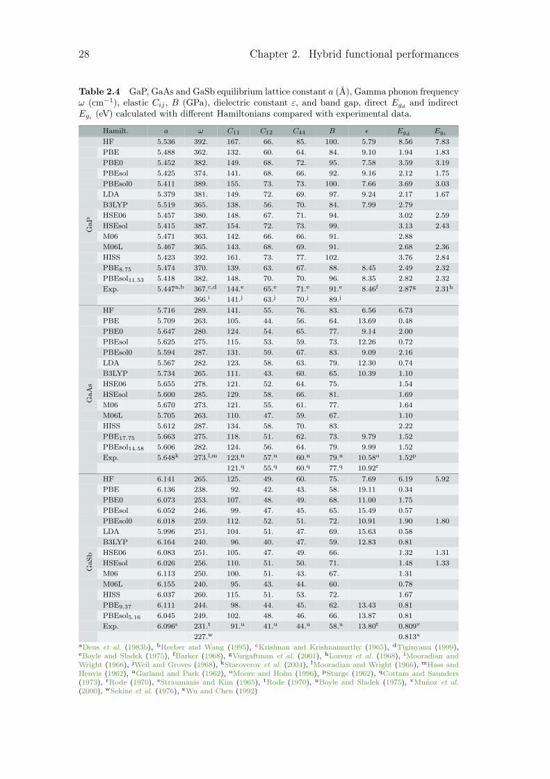
Table 2.4 GaP, GaAs and GaSb equilibrium lattice constant a (Å), Gamma phonon frequencyω (cm−1), elastic Cij , B (GPa), dielectric constant ε, and band gap, direct Egd and indirectEgi (eV) calculated with different Hamiltonians compared with experimental data.
Hamilt. a ω C11 C12 C44 B ε Egd EgiHF 5.536 392. 167. 66. 85. 100. 5.79 8.56 7.83
PBE 5.488 362. 132. 60. 64. 84. 9.10 1.94 1.83
PBE0 5.452 382. 149. 68. 72. 95. 7.58 3.59 3.19
PBEsol 5.425 374. 141. 68. 66. 92. 9.16 2.12 1.75
PBEsol0 5.411 389. 155. 73. 73. 100. 7.66 3.69 3.03
LDA 5.379 381. 149. 72. 69. 97. 9.24 2.17 1.67
B3LYP 5.519 365. 138. 56. 70. 84. 7.99 2.79
HSE06 5.457 380. 148. 67. 71. 94. 3.02 2.59
HSEsol 5.415 387. 154. 72. 73. 99. 3.13 2.43
M06 5.471 363. 142. 66. 66. 91. 2.88
M06L 5.467 365. 143. 68. 69. 91. 2.68 2.36
HISS 5.423 392. 161. 73. 77. 102. 3.76 2.84
PBE8.75 5.474 370. 139. 63. 67. 88. 8.45 2.49 2.32
PBEsol11.53 5.418 382. 148. 70. 70. 96. 8.35 2.82 2.32
Exp. 5.447a,b 367.c,d 144.e 65.e 71.e 91.e 8.46f 2.87g 2.31h
GaP
366.i 141.j 63.j 70.j 89.j
HF 5.716 289. 141. 55. 76. 83. 6.56 6.73
PBE 5.709 263. 105. 44. 56. 64. 13.69 0.48
PBE0 5.647 280. 124. 54. 65. 77. 9.14 2.00
PBEsol 5.625 275. 115. 53. 59. 73. 12.26 0.72
PBEsol0 5.594 287. 131. 59. 67. 83. 9.09 2.16
LDA 5.567 282. 123. 58. 63. 79. 12.30 0.74
B3LYP 5.734 265. 111. 43. 60. 65. 10.39 1.10
HSE06 5.655 278. 121. 52. 64. 75. 1.54
HSEsol 5.600 285. 129. 58. 66. 81. 1.69
M06 5.670 273. 121. 55. 61. 77. 1.64
M06L 5.705 263. 110. 47. 59. 67. 1.10
HISS 5.612 287. 134. 58. 70. 83. 2.22
PBE17.75 5.663 275. 118. 51. 62. 73. 9.79 1.52
PBEsol14.58 5.606 282. 124. 56. 64. 79. 9.99 1.52
Exp. 5.648k 273.l,m 123.n 57.n 60.n 79.n 10.58o 1.52p
GaA
s
121.q 55.q 60.q 77.q 10.92r
HF 6.141 265. 125. 49. 60. 75. 7.69 6.19 5.92
PBE 6.136 238. 92. 42. 43. 58. 19.11 0.34
PBE0 6.073 253. 107. 48. 49. 68. 11.00 1.75
PBEsol 6.052 246. 99. 47. 45. 65. 15.49 0.57
PBEsol0 6.018 259. 112. 52. 51. 72. 10.91 1.90 1.80
LDA 5.996 251. 104. 51. 47. 69. 15.63 0.58
B3LYP 6.164 240. 96. 40. 47. 59. 12.83 0.81
HSE06 6.083 251. 105. 47. 49. 66. 1.32 1.31
HSEsol 6.026 256. 110. 51. 50. 71. 1.48 1.33
M06 6.113 250. 100. 51. 43. 67. 1.31
M06L 6.155 240. 95. 43. 44. 60. 0.78
HISS 6.037 260. 115. 51. 53. 72. 1.67
PBE9.37 6.111 244. 98. 44. 45. 62. 13.43 0.81
PBEsol5.16 6.045 249. 102. 48. 46. 66. 13.87 0.81
Exp. 6.096s 231.t 91.u 41.u 44.u 58.u 13.80t 0.809v
GaS
b
227.w 0.813x
aDeus et al. (1983b), bReeber and Wang (1995), cKrishnan and Krishnamurthy (1965), dTiginyanu (1999),eBoyle and Sladek (1975), fBarker (1968), gVurgaftman et al. (2001), hLorenz et al. (1968), iMooradian andWright (1966), jWeil and Groves (1968), kStaroverov et al. (2004), lMooradian and Wright (1966), mHass andHenvis (1962), nGarland and Park (1962), oMoore and Holm (1996), pSturge (1962), qCottam and Saunders(1973), rRode (1970), sStraumanis and Kim (1965), tRode (1970), uBoyle and Sladek (1975), vMuñoz et al.(2000), wSekine et al. (1976), xWu and Chen (1992)
2.1. Hybrid functionals 29
0.0 0.5 1.0 1.5 2.0
HFB3LYP
LDAPBE
PBEsol0HSEsol
PBEsolhyb
PBEhyb
M06HISS
PBEsolM06L
HSE06PBE0
a
GaP 0 5 10 15 20
HISSHFPBEsol0
HSEsolPBEB3LYP
LDA
PBEsolhyb
PBE0HSE06
PBEhyb
PBEsolM06M06L
B
0 100 200
HFPBEHISSPBEsol0PBEsolPBE0LDA
PBEhyb
HSEsolM06LHSE06B3LYP
PBEsolhyb
M06 Egd
0.0 2.5 5.0 7.5 10.0
HFHISS
PBEsol0HSEsol
PBE0
PBEsolhyb
LDAHSE06
PBEsolPBE
M06
PBEhyb
B3LYPM06L
ω
0 10 20 30 40
HFPBE0
PBEsol0LDA
PBEsolPBE
B3LYP
PBEsolhyb
PBEhyb
ε
0 100 200 300
HFPBE0
PBEsol0LDAPBEsolHISSPBE
HSE06HSEsolM06L
PBEhyb
PBEsolhyb Egi
0.0 0.5 1.0 1.5 2.0
B3LYPLDA
HFPBE
M06LPBEsol0
HSEsol
PBEsolhyb
HISSPBEsolM06
PBEhyb
HSE06PBE0
a
GaAs 0 10 20
PBEB3LYP
M06LHFPBEsol0HISS
PBEsolHSEsol
PBEhyb
LDAHSE06
PBEsolhyb
PBE0M06
B
0 200 400
HFPBE
PBEsolLDAHISSPBEsol0
PBE0B3LYPM06L
HSEsolM06HSE06
PBEhyb
PBEsolhyb Egd
0 2 4 6 8
HFPBEsol0HISS
HSEsolPBEM06L
LDA
PBEsolhyb
B3LYPPBE0
HSE06PBEsol
PBEhyb
M06
ω
0 20 40
HFPBE
LDAPBEsol
PBEsol0PBE0
PBEhyb
PBEsolhyb
B3LYP
ε
0.0 0.5 1.0 1.5 2.0
LDAPBEsol0
HSEsolB3LYP
M06LHISS
PBEsolhyb
HFPBEsol
PBEPBE0
M06
PBEhyb
HSE06
a
GaSb 0 20 40
HFPBEsol0HISS
HSEsolLDA
PBE0M06
HSE06
PBEsolhyb
PBEsol
PBEhyb
M06LB3LYP
PBE
B
0 200 400 600 800
HFPBEsol0
PBE0HISS
HSEsolHSE06M06PBE
PBEsolLDA
M06LB3LYP
PBEhyb
PBEsolhyb Egd
0 5 10 15 20
HFHISS
PBEsol0HSEsol
PBE0LDAHSE06
M06
PBEsolhyb
PBEsol
PBEhyb
B3LYPM06L
PBE
ω
0 20 40 60
HFPBE
PBEsol0PBE0
LDAPBEsol
B3LYP
PBEhyb
PBEsolhyb
ε
Relative error / %
Figure 2.6 Absolute value of the relative error between calculated and experimental proper-ties of GaP, GaAs and GaSb for each Hamiltonian.Hybrid functionals optimised for the materialare displayed in orange.

30 Chapter 2. Hybrid functional performances
Table 2.5 InP, InAs and InSb equilibrium lattice constant a (Å), Gamma phonon frequencyω (cm−1), elastic Cij , B (GPa), dielectric constant ε, and band gap, direct Egd and indirectEgi (eV) calculated with different Hamiltonians compared with experimental data.
Hamilt. a ω C11 C12 C44 B ε EgdHF 5.974 327. 126. 61. 61. 83. 10.41 6.70
PBEXC 5.971 297. 93. 48. 44. 63. 7.67 0.61
PBE0 5.910 316. 109. 58. 50. 75. 10.16 2.08
PBESOLXC 5.897 309. 100. 55. 45. 70. 7.74 0.72
PBESOL0 5.864 324. 114. 62. 51. 79. 10.32 2.11
SVWN 5.851 315. 105. 59. 47. 74. 8.49 0.70
B3LYP 5.995 300. 98. 48. 48. 64. 8.57 1.32
HSE06 5.915 315. 107. 57. 50. 73. 1.54
HSESOL 5.869 322. 112. 61. 50. 78. 1.59
M06 5.941 306. 103. 57. 44. 72. 1.55
M06L 5.957 289. 97. 53. 44. 69. 1.25
HISS 5.874 326. 118. 62. 54. 81. 2.13
PBE14.81 5.931 309. 102. 54. 48. 70. 8.38 1.42
PBEsol13.23 5.877 317. 108. 59. 49. 75. 8.55 1.42
Exp. 5.866a 308.b 102.c 58.c 46.c,d 73.c 9.56e 1.42f,g
InP
101.d 56.d 71.d
HF 6.136 226. 108. 52. 55. 69. 6.24 5.47
PBEXC 6.171 204. 75. 39. 36. 50. 15.29
PBE0 6.087 222. 91. 48. 43. 61. 9.83 0.88
PBESOLXC 6.077 214. 83. 46. 38. 57. 14.39
PBESOL0 6.030 228. 97. 53. 45. 66. 9.72 0.94
SVWN 6.020 220. 89. 50. 40. 62. 14.67
B3LYP 6.186 210. 81. 38. 41. 51. 97.39 0.10
HSE06 6.096 220. 89. 47. 42. 60. 0.46
HSESOL 6.038 227. 95. 51. 44. 65. 0.52
M06 6.133 220. 88. 46. 40. 59. 0.55
M06L 6.198 201. 75. 40. 36. 50.
HISS 6.047 228. 99. 52. 47. 66. 0.99
PBE17.08 6.110 217. 86. 45. 41. 58. 13.01 0.41
PBEsol15.47 6.047 224. 92. 50. 42. 63. 13.15 0.41
Exp. 6.058h 220.i 90.j 50.j 39.j 63.j 11.78k 0.41l
InAs
83.m 45.m 40.m
HF 6.524 211. 102. 47. 47. 63. 7.20 5.39
PBEXC 6.548 186. 71. 37. 31. 47. 16.42
PBE0 6.468 202. 85. 44. 37. 56. 10.87 1.08
PBESOLXC 6.457 194. 77. 42. 33. 52. 0.01
PBESOL0 6.410 206. 89. 47. 38. 60. 10.77 1.19
SVWN 6.402 197. 81. 44. 34. 56. 15.92
B3LYP 6.571 191. 76. 36. 35. 48. 17.35 0.29
HSE06 6.478 200. 83. 43. 36. 55. 0.71
HSESOL 6.418 205. 88. 46. 37. 58. 0.81
M06 6.544 200. 77. 43. 31. 53. 0.61
M06L 6.590 189. 72. 38. 31. 48. 0.14
HISS 6.426 207. 92. 47. 40. 60. 1.22
PBE9.05 6.516 194. 77. 40. 33. 50. 21.89 0.23
PBEsol5.73 6.445 199. 80. 43. 34. 54. 22.99 0.23
Exp. 6.479n 182.o 67.p 34.p 31.p,q 45.p 16.76r 0.23s
InSb
69.q 38.q
aReeber andWang (1995), bMooradian andWright (1966), cHickernell and Gayton (1966), dNichols et al. (1980),eRode (1970), fPavesi et al. (1991), gVarshni (1967) hIoffe Institute (2019), iCarles et al. (1980), jGerlich (1964),kRode (1970), lFang et al. (1990), mGerlich (1963) nStraumanis and Kim (1965), oKiefer et al. (1975), pPotter(1956), qSlutsky and Garland (1959), rRode (1970), sZollner et al. (1991)
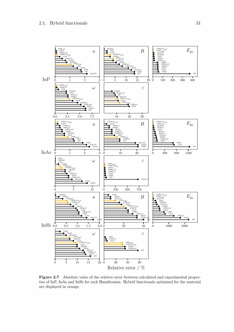
2.1. Hybrid functionals 31
0 1 2 3
B3LYPHF
PBEM06L
M06
PBEhyb
HSE06PBE0
PBEsolLDA
PBEsolhyb
PBEsol0HISS
HSEsol
a
InP 0 5 10 15 20
HFPBE
B3LYPHISS
PBEsol0HSEsol
M06LPBEsol
PBEhyb
PBE0
PBEsolhyb
LDAM06
HSE06
B
0 100 200 300 400
HFPBELDAHISSPBEsolPBEsol0PBE0
HSEsolM06LM06HSE06B3LYP
PBEhyb
PBEsolhyb Egd
0.0 2.5 5.0 7.5
HFM06L
HISSPBEsol0
HSEsolPBE
PBEsolhyb
PBE0B3LYP
LDAHSE06
M06PBEsol
PBEhyb
ω
10 20 30
PBEPBEsol
PBEhyb
LDA
PBEsolhyb
B3LYPHF
PBEsol0PBE0
ε
0 1 2 3
M06LB3LYP
PBEHF
M06
PBEhyb
LDAHSE06
PBE0PBEsol0
HSEsolPBEsol
HISS
PBEsolhyb
a
InAs 0 10 20
PBEM06L
B3LYPHFPBEsol
PBEhyb
M06PBEsol0HSE06HISS
PBE0HSEsol
LDA
PBEsolhyb
B
0 400 800 1200
HFLDA
PBEHISSPBEsol0PBE0PBEsol
B3LYPM06L
M06HSEsolHSE06
PBEhyb
PBEsolhyb Egd
0 5 10
M06LPBE
B3LYPPBEsol0HISS
HSEsolHFPBEsol
PBEsolhyb
PBEhyb
PBE0LDAHSE06M06
ω
0 250 500 750
B3LYPHF
PBELDAPBEsolPBEsol0PBE0
PBEsolhyb
PBEhyb
ε
0.0 0.5 1.0 1.5 2.0
M06LB3LYP
LDAPBEPBEsol0
M06HSEsol
HISSHF
PBEhyb
PBEsolhyb
PBEsolPBE0
HSE06
a
InSb 0 20 40
HFPBEsol0HISS
HSEsolPBE0LDA
HSE06
PBEsolhyb
M06PBEsol
PBEhyb
B3LYPM06L
PBE
B
0 1000 2000
HFM06L
PBEsolLDA
PBEHISSPBEsol0
PBE0HSEsol
HSE06M06
B3LYP
PBEhyb
PBEsolhyb Egd
0 5 10 15 20
HFHISS
PBEsol0HSEsol
PBE0HSE06M06
PBEsolhyb
LDAPBEsol
PBEhyb
B3LYPM06L
PBE
ω
0 20 40 60
HFPBEsol0PBE0
PBEsolhyb
PBEhyb
LDAB3LYP
PBE
ε
Relative error / %
Figure 2.7 Absolute value of the relative error between calculated and experimental proper-ties of InP, InAs and InSb for each Hamiltonian. Hybrid functionals optimised for the materialare displayed in orange.
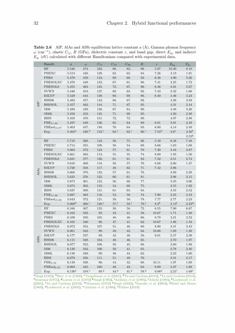
32 Chapter 2. Hybrid functional performances
Table 2.6 AlP, AlAs and AlSb equilibrium lattice constant a (Å), Gamma phonon frequencyω (cm−1), elastic Cij , B (GPa), dielectric constant ε, and band gap, direct Egd and indirectEgi (eV) calculated with different Hamiltonians compared with experimental data.
Hamilt. a ω C11 C12 C44 B ε Egd EgiHF 5.540 474. 162. 68. 83. 99. 5.07 10.30 8.10
PBEXC 5.513 440. 129. 62. 62. 84. 7.26 3.19 1.91
PBE0 5.479 459. 143. 69. 68. 93. 6.38 4.90 3.20
PBESOLXC 5.476 448. 132. 67. 61. 88. 7.41 3.25 1.72
PBESOL0 5.455 463. 145. 72. 67. 96. 6.46 4.91 3.07
SVWN 5.440 453. 137. 69. 63. 92. 7.43 3.32 1.68
B3LYP 5.529 444. 138. 60. 69. 86. 6.40 4.46 3.23
HSE06 5.482 457. 142. 68. 67. 92. 4.28 2.58
HSESOL 5.457 462. 144. 71. 67. 95. 4.31 2.44
M06 5.489 429. 138. 67. 64. 90. 4.46 3.26
M06L 5.456 452. 145. 71. 69. 95. 4.20 2.30
HISS 5.459 470. 151. 72. 72. 99. 4.97 2.88
PBE11.50 5.497 449. 136. 65. 64. 89. 6.81 3.91 2.49
PBEsol14.57 5.463 457. 140. 70. 64. 93. 6.80 4.14 2.49
Exp. 5.464a 440.b 133.c 63.c 62.c 86.c 7.54d 3.6e 2.50f
AlP
2.52g
HF 5.710 380. 142. 58. 75. 86. 5.49 8.48 7.48
PBEXC 5.714 355. 109. 50. 54. 69. 8.66 1.83 1.68
PBE0 5.663 372. 123. 57. 61. 79. 7.30 3.44 2.87
PBESOLXC 5.661 363. 113. 55. 55. 74. 8.69 1.95 1.50
PBESOL0 5.631 377. 126. 61. 61. 82. 7.32 3.51 2.74
SVWN 5.616 369. 118. 58. 57. 78. 8.68 2.00 1.47
B3LYP 5.720 358. 117. 48. 62. 71. 7.42 2.86
HSE06 5.668 370. 122. 57. 61. 78. 2.89 2.28
HSESOL 5.635 376. 125. 60. 61. 81. 2.96 2.15
M06 5.673 361. 122. 56. 60. 77. 3.25 3.06
M06L 5.674 362. 118. 54. 60. 75. 2.55 1.92
HISS 5.637 380. 131. 61. 65. 84. 3.55 2.52
PBE11.96 5.687 363. 116. 53. 58. 74. 7.90 2.45 2.23
PBEsol15.02 5.643 372. 121. 59. 59. 79. 7.77 2.77 2.23
AlA
s
Exp. 5.660h 360.i 120.j 57.j 59.j 78.j 8.2k 3.13l 2.23m
HF 6.166 367. 123. 50. 58. 72. 6.55 7.90 6.67
PBEXC 6.162 333. 93. 43. 41. 58. 10.67 1.71 1.46
PBE0 6.109 350. 105. 48. 46. 66. 8.79 3.21 2.52
PBESOLXC 6.105 340. 96. 47. 41. 62. 10.67 1.86 1.33
PBESOL0 6.072 354. 107. 51. 46. 68. 8.80 3.31 2.43
SVWN 6.061 343. 99. 49. 42. 64. 10.66 1.89 1.30
B3LYP 6.177 337. 99. 42. 46. 59. 9.01 2.57 2.39
HSE06 6.115 348. 104. 48. 46. 65. 2.70 1.97
HSESOL 6.077 352. 106. 50. 45. 68. 2.80 1.88
M06 6.130 342. 100. 50. 41. 65. 2.78 2.40
M06L 6.138 340. 99. 46. 44. 62. 2.23 1.60
HISS 6.079 358. 111. 51. 49. 70. 3.31 2.17
PBE5.70 6.149 338. 96. 44. 42. 60. 10.11 1.97 1.69
PBEsol8.53 6.093 345. 100. 48. 43. 64. 9.89 2.27 1.69
AlSb
Exp. 6.136n 318.o 89.p 44.p 41.p 59.p 9.88q 2.21r 1.69s
aSingh (1992), bBeer et al. (1968), cVurgaftman et al. (2001), dYu and Cardona (2010), eYu and Cardona (2010),fMonemar (1973), gLorenz et al. (1970) hSingh (1992), iAzuhata et al. (1995), jAdachi (1985), kLockwood et al.(2005), lYu and Cardona (2010), mMonemar (1973) nSingh (1992), oIsaenko et al. (2003), pBolef and Menes(1960), qLockwood et al. (2005), rCardona et al. (1966), sPalmer (2019)

2.1. Hybrid functionals 33
0.0 0.5 1.0 1.5 2.0
HFB3LYP
PBE
PBEhyb
M06LDA
HSE06PBE0
PBEsolPBEsol0M06LHSEsol
HISS
PBEsolhyb
a
AlP 0 5 10 15 20
HFHISS
PBEsol0HSEsolM06L
PBE0
PBEsolhyb
LDAHSE06
M06
PBEhyb
PBEPBEsol
B3LYP
B
0 100 200
HFPBE
LDAPBEsol
HISSPBEsol0PBE0
M06LB3LYPM06
HSEsolHSE06
PBEsolhyb
PBEhyb Egd
0 5 10
HFHISS
PBEsol0HSEsol
PBE0HSE06
PBEsolhyb
LDAM06L
M06
PBEhyb
PBEsolB3LYP
PBE
ω
0 20 40 60
HFPBE0B3LYPPBEsol0
PBEsolhyb
PBEhyb
PBEPBEsolLDA
ε
0 100 200 300
HFLDAPBEsolM06B3LYPPBE0
PBEPBEsol0
HISSM06L
HSE06HSEsol
PBEhyb
PBEsolhyb Egi
0.0 0.5 1.0 1.5
B3LYPPBE
HFLDA
PBEsol0
PBEhyb
HSEsolHISS
PBEsolhyb
M06LM06
HSE06PBE0
PBEsol
a
AlAs 0 5 10 15
PBEHF
B3LYPHISS
PBEsolPBEsol0
PBEhyb
HSEsolM06L
PBE0M06
PBEsolhyb
LDAHSE06
B
0 100 200
HFPBEsol
M06L
PBEhyb
HISSPBEsol0
PBEsolhyb
PBE0B3LYPHSE06HSEsolM06 Egd
0 2 4 6 8
HFHISS
PBEsol0HSEsol
PBE0
PBEsolhyb
HSE06LDA
PBEPBEsol
PBEhyb
B3LYPM06L
M06
ω
0 20 40
HFPBE0PBEsol0
B3LYPPBEsolLDAPBE
PBEsolhyb
PBEhyb
ε
0 100 200 300
HFM06LDAPBEsolPBE0PBEPBEsol0
M06LHISS
B3LYPHSEsolHSE06
PBEhyb
PBEsolhyb Egi
0.0 0.5 1.0 1.5
LDAPBEsol0
HSEsolHISS
PBEsolhyb
B3LYPPBEsolHF
PBE0PBE
HSE06
PBEhyb
M06M06L
a
AlSb 0 10 20 30
HFHISS
PBEsol0HSEsol
PBE0HSE06M06
LDA
PBEsolhyb
PBEsolM06L
PBE
PBEhyb
B3LYP
B
0 100 200 300
HFPBEsol0HISSPBE0
HSEsolM06HSE06
B3LYP
PBEhyb
PBEsolhybEgd
0 5 10 15 20
HFHISS
PBEsol0HSEsol
PBE0HSE06
PBEsolhyb
LDAM06
PBEsolM06L
PBEhyb
B3LYPPBE
ω
0 10 20 30 40
HFPBE0PBEsol0
B3LYPPBEPBEsolLDA
PBEhyb
PBEsolhyb
ε
Relative error / %0 100 200 300
HFPBE0
PBEsol0M06
HISSLDAPBEsolHSE06PBEHSEsol
M06L
PBEhyb
PBEsolhyb Egi
Figure 2.8 Absolute value of the relative error between calculated and experimental proper-ties of AlP, AlAs and AlSb for each Hamiltonian.Hybrid functionals optimised for the materialare displayed in orange.
34 Chapter 2. Hybrid functional performances
this different properties and defined a global error for the structural parameters.The same procedure have been done for the other properties. Thus, we found thebulk modulus, the electrical properties corresponding to the average error for di-rect and indirect band gap, the dielectric properties which regroup the dielectricconstant and the vibrational frequencies. Even though all this properties are notdirectly comparable, we summed their relative errors with experiments to have aglobal point of view of the functional’s performances. As the hybrid functionaldeveloped in this work correctly reproduced the experimental band gap, the rel-ative error for the electronic properties only comes from the divergence betweenthe calculated and experimental values of the direct band gap of indirect-bandgap semiconductors. This error is then extremely small compared to the otherfunctionals from literature. We then define the measure of two distinct globalerrors for every Hamiltonian. The first one, called MAREtot, is the average er-ror throughout all properties. The second one, called MARE0, is the same asMAREtot without the contribution of the electronic properties’ error.
As expected, the Hartree-Fock Hamiltonian leads to an overestimation of theband gap (350%) when LDA and GGA functionals underestimate its value, giving40% and 43% respectively. PBEhyb and PBEsolhyb obviously give the best resultsfor the band gap. B3LYP was created for organic molecular systems with covalentbonds. The high number of covalent materials among our test cases explainstherefore that the mean B3LYP energy is low. However, B3LYP wrongly predictsthe band gap to be direct for GaP and AlAs. PBEsol, HSe06 and M06 are theother functionals that lead to the lowest MARE, around 19%. When looking atthe structural properties, PBE and PBEsol functionals have the lowest MARE.This is why the MARE of PBEhyb and PBEsolhyb is better than the majority ofthe other functionals with only 0.5 %. This is not the case for the precision inthe bulk modulus calculation where PBEhyb is in the average error of the otherfunctionals and PBEsolhyb is among those with the highest error. Just as forthe lattice parameters, PBE gives the lowest MARE. Nonetheless, these resultsare less significant because of the experimental precision of the bulk modulusthat is often of the order of several tens of percent. The dielectric propertiescalculated with PBEhyb and PBEsolhyb are very close to the experimental datawith less than a 5% error. The other functionals tested give results from 10%to more than 30% for PBEsol. This comparison is not complete as the coupled-perturbed Kohn-Sham/Hartree-Fock (CPKS/HF) method is not implemented forseveral functionals used here. Finally, the last properties studied were the Gammavibration frequencies of the crystal. Once again, PBE has the smallest MAREwhich is 0.39%. All the MARE are less or equal to 10%. In this context, thetwo optimised hybrid functionals do not give significant result compared to theother functionals with 3% and 5% for PBEhyb and PBEsolhyb respectively. Thepenultimate column is the average value for all the properties of each functional.Thanks to their performance for the calculation of the band gap, PBEhyb andPBEsolhyb give the lowest relative error. However, if we exclude the electronicproperties of the mean values as in the last colum (MARE0), these two optimisedhybrid functionals are still the most accurate ones included in the tests, withrelative errors of 6% and 9% just as LDA, HSE06 and the M06 functionals.
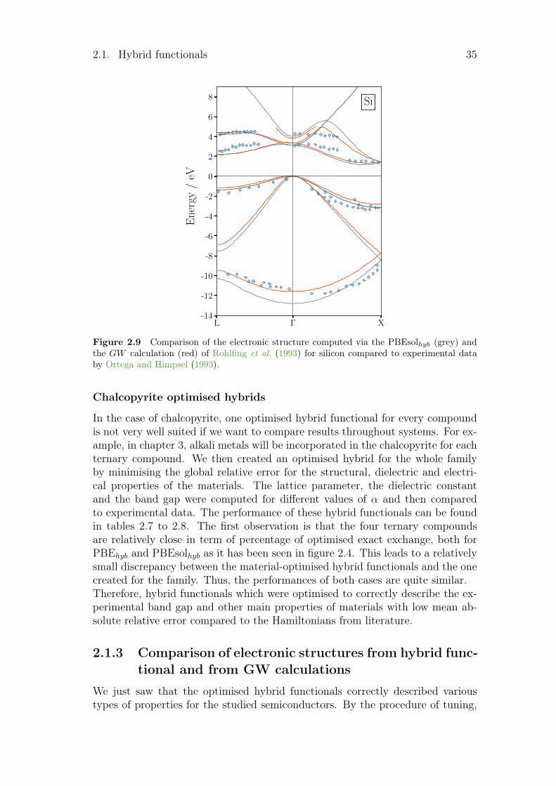
2.1. Hybrid functionals 35
L Γ X-14
-12
-10
-8
-6
-4
-2
0
2
4
6
8 Si
En
ergy
/eV
Figure 2.9 Comparison of the electronic structure computed via the PBEsolhyb (grey) andthe GW calculation (red) of Rohlfing et al. (1993) for silicon compared to experimental databy Ortega and Himpsel (1993).
Chalcopyrite optimised hybrids
In the case of chalcopyrite, one optimised hybrid functional for every compoundis not very well suited if we want to compare results throughout systems. For ex-ample, in chapter 3, alkali metals will be incorporated in the chalcopyrite for eachternary compound. We then created an optimised hybrid for the whole familyby minimising the global relative error for the structural, dielectric and electri-cal properties of the materials. The lattice parameter, the dielectric constantand the band gap were computed for different values of α and then comparedto experimental data. The performance of these hybrid functionals can be foundin tables 2.7 to 2.8. The first observation is that the four ternary compoundsare relatively close in term of percentage of optimised exact exchange, both forPBEhyb and PBEsolhyb as it has been seen in figure 2.4. This leads to a relativelysmall discrepancy between the material-optimised hybrid functionals and the onecreated for the family. Thus, the performances of both cases are quite similar.Therefore, hybrid functionals which were optimised to correctly describe the ex-perimental band gap and other main properties of materials with low mean ab-solute relative error compared to the Hamiltonians from literature.
2.1.3 Comparison of electronic structures from hybrid func-tional and from GW calculations
We just saw that the optimised hybrid functionals correctly described varioustypes of properties for the studied semiconductors. By the procedure of tuning,
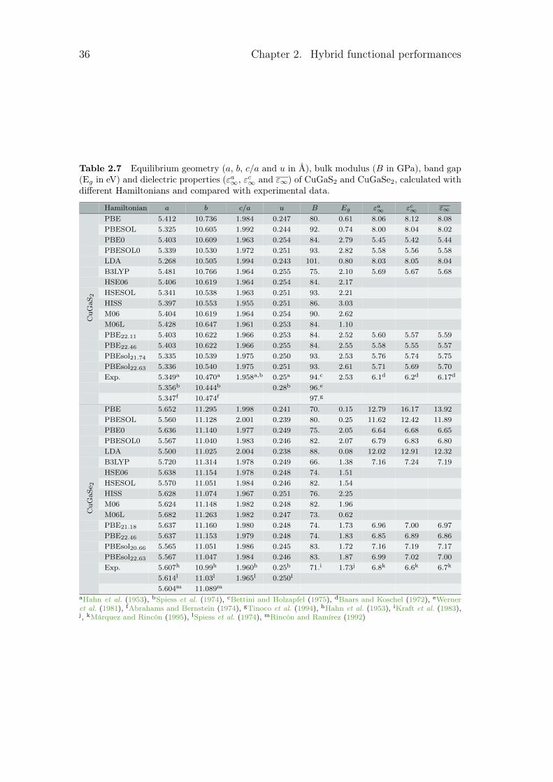
36 Chapter 2. Hybrid functional performances
Table 2.7 Equilibrium geometry (a, b, c/a and u in Å), bulk modulus (B in GPa), band gap(Eg in eV) and dielectric properties (εa∞, εc∞ and ε∞) of CuGaS2 and CuGaSe2, calculated withdifferent Hamiltonians and compared with experimental data.
Hamiltonian a b c/a u B Eg εa∞ εc∞ ε∞
PBE 5.412 10.736 1.984 0.247 80. 0.61 8.06 8.12 8.08
PBESOL 5.325 10.605 1.992 0.244 92. 0.74 8.00 8.04 8.02
PBE0 5.403 10.609 1.963 0.254 84. 2.79 5.45 5.42 5.44
PBESOL0 5.339 10.530 1.972 0.251 93. 2.82 5.58 5.56 5.58
LDA 5.268 10.505 1.994 0.243 101. 0.80 8.03 8.05 8.04
B3LYP 5.481 10.766 1.964 0.255 75. 2.10 5.69 5.67 5.68
HSE06 5.406 10.619 1.964 0.254 84. 2.17
HSESOL 5.341 10.538 1.963 0.251 93. 2.21
HISS 5.397 10.553 1.955 0.251 86. 3.03
M06 5.404 10.619 1.964 0.254 90. 2.62
M06L 5.428 10.647 1.961 0.253 84. 1.10
PBE22.11 5.403 10.622 1.966 0.253 84. 2.52 5.60 5.57 5.59
PBE22.46 5.403 10.622 1.966 0.255 84. 2.55 5.58 5.55 5.57
PBEsol21.74 5.335 10.539 1.975 0.250 93. 2.53 5.76 5.74 5.75
PBEsol22.63 5.336 10.540 1.975 0.251 93. 2.61 5.71 5.69 5.70
Exp. 5.349a 10.470a 1.958a,b 0.25a 94.c 2.53 6.1d 6.2d 6.17d
5.356b 10.444b 0.28b 96.e
CuG
aS2
5.347f 10.474f 97.g
PBE 5.652 11.295 1.998 0.241 70. 0.15 12.79 16.17 13.92
PBESOL 5.560 11.128 2.001 0.239 80. 0.25 11.62 12.42 11.89
PBE0 5.636 11.140 1.977 0.249 75. 2.05 6.64 6.68 6.65
PBESOL0 5.567 11.040 1.983 0.246 82. 2.07 6.79 6.83 6.80
LDA 5.500 11.025 2.004 0.238 88. 0.08 12.02 12.91 12.32
B3LYP 5.720 11.314 1.978 0.249 66. 1.38 7.16 7.24 7.19
HSE06 5.638 11.154 1.978 0.248 74. 1.51
HSESOL 5.570 11.051 1.984 0.246 82. 1.54
HISS 5.628 11.074 1.967 0.251 76. 2.25
M06 5.624 11.148 1.982 0.248 82. 1.96
M06L 5.682 11.263 1.982 0.247 73. 0.62
PBE21.18 5.637 11.160 1.980 0.248 74. 1.73 6.96 7.00 6.97
PBE22.46 5.637 11.153 1.979 0.248 74. 1.83 6.85 6.89 6.86
PBEsol20.66 5.565 11.051 1.986 0.245 83. 1.72 7.16 7.19 7.17
PBEsol22.63 5.567 11.047 1.984 0.246 83. 1.87 6.99 7.02 7.00
Exp. 5.607h 10.99h 1.960h 0.25h 71.i 1.73j 6.8k 6.6k 6.7k
5.614l 11.03l 1.965l 0.250l
CuG
aSe 2
5.604m 11.089m
aHahn et al. (1953), bSpiess et al. (1974), cBettini and Holzapfel (1975), dBaars and Koschel (1972), eWerneret al. (1981), fAbrahams and Bernstein (1974), gTinoco et al. (1994), hHahn et al. (1953), iKraft et al. (1983),j, kMárquez and Rincón (1995), lSpiess et al. (1974), mRincón and Ramírez (1992)
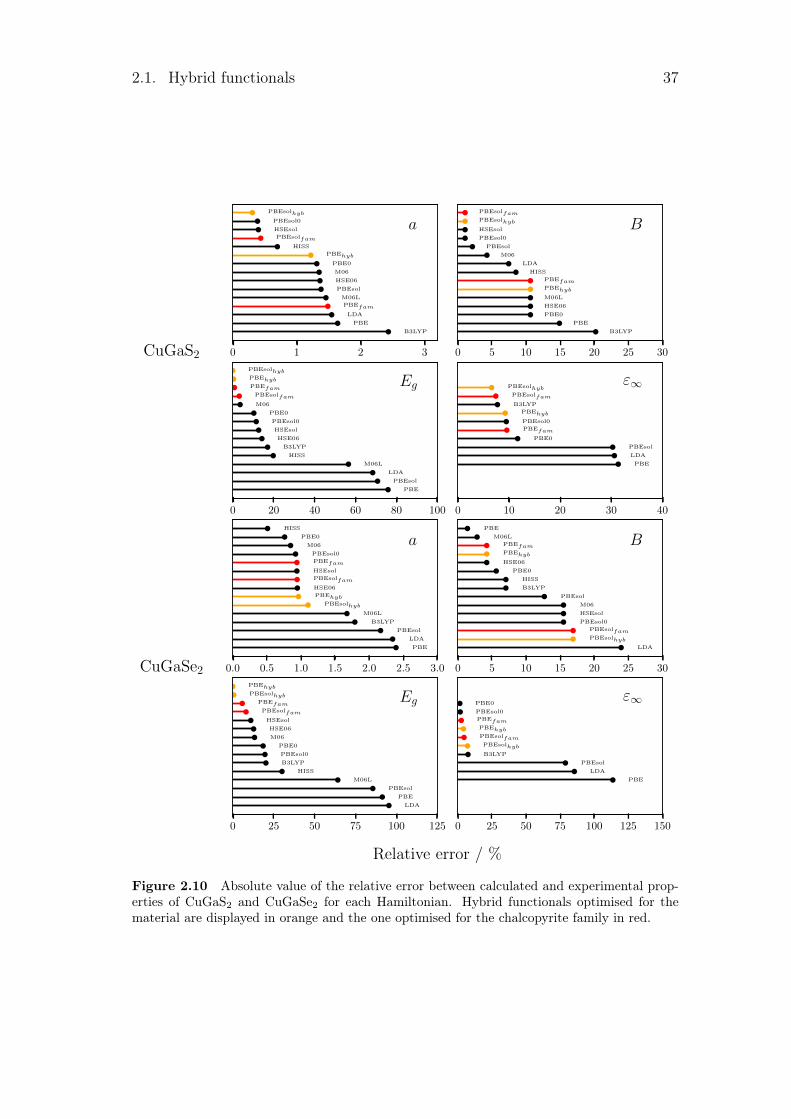
2.1. Hybrid functionals 37
0 1 2 3
B3LYP
PBE
LDA
PBEfam
M06L
PBEsol
HSE06
M06
PBE0
PBEhyb
HISS
PBEsolfam
HSEsol
PBEsol0
PBEsolhyb
a
CuGaS2 0 5 10 15 20 25 30
B3LYP
PBE
PBE0
HSE06
M06L
PBEhyb
PBEfam
HISS
LDA
M06
PBEsol
PBEsol0
HSEsol
PBEsolhyb
PBEsolfam
B
0 20 40 60 80 100
PBE
PBEsol
LDA
M06L
HISS
B3LYP
HSE06
HSEsol
PBEsol0
PBE0
M06
PBEsolfam
PBEfam
PBEhyb
PBEsolhyb
Eg
0 10 20 30 40
PBE
LDA
PBEsol
PBE0
PBEfam
PBEsol0
PBEhyb
B3LYP
PBEsolfam
PBEsolhybε∞
0.0 0.5 1.0 1.5 2.0 2.5 3.0
PBE
LDA
PBEsol
B3LYP
M06L
PBEsolhyb
PBEhyb
HSE06
PBEsolfam
HSEsol
PBEfam
PBEsol0
M06
PBE0
HISS
a
CuGaSe2 0 5 10 15 20 25 30
LDA
PBEsolhyb
PBEsolfam
PBEsol0
HSEsol
M06
PBEsol
B3LYP
HISS
PBE0
HSE06
PBEhyb
PBEfam
M06L
PBE
B
0 25 50 75 100 125
LDA
PBE
PBEsol
M06L
HISS
B3LYP
PBEsol0
PBE0
M06
HSE06
HSEsol
PBEsolfam
PBEfam
PBEsolhyb
PBEhyb
Eg
Relative error / %
0 25 50 75 100 125 150
PBE
LDA
PBEsol
B3LYP
PBEsolhyb
PBEsolfam
PBEhyb
PBEfam
PBEsol0
PBE0ε∞
Figure 2.10 Absolute value of the relative error between calculated and experimental prop-erties of CuGaS2 and CuGaSe2 for each Hamiltonian. Hybrid functionals optimised for thematerial are displayed in orange and the one optimised for the chalcopyrite family in red.
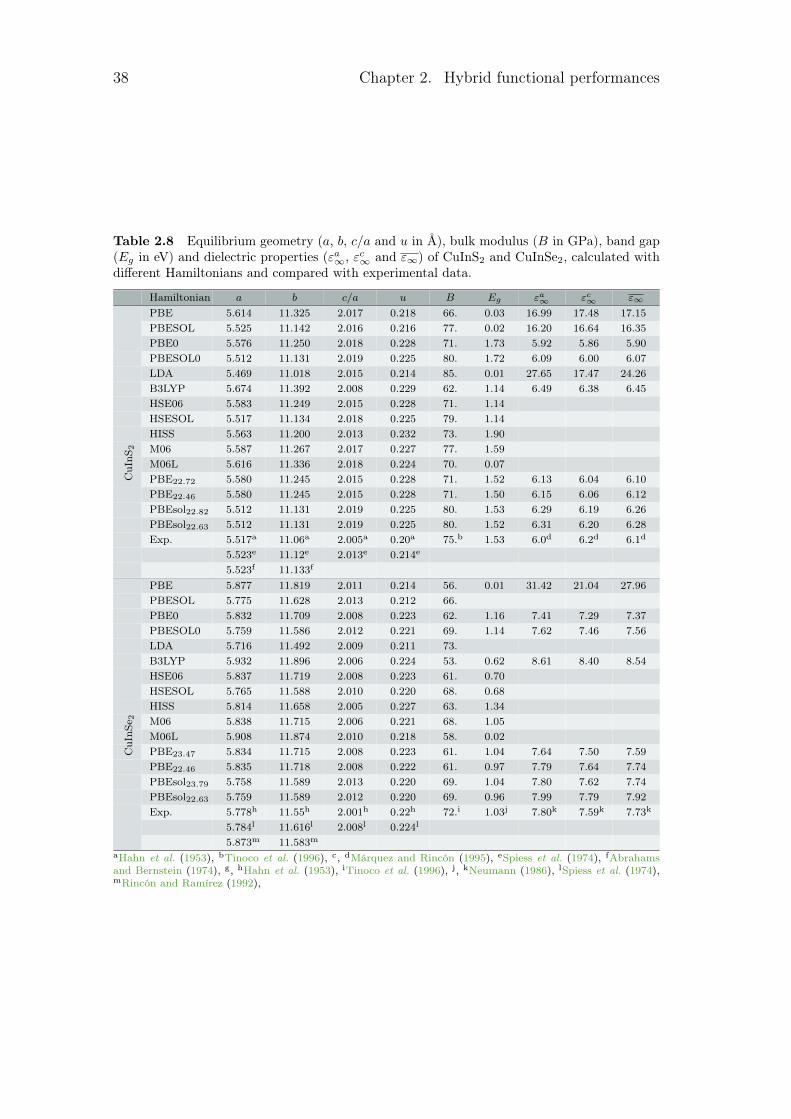
38 Chapter 2. Hybrid functional performances
Table 2.8 Equilibrium geometry (a, b, c/a and u in Å), bulk modulus (B in GPa), band gap(Eg in eV) and dielectric properties (εa∞, εc∞ and ε∞) of CuInS2 and CuInSe2, calculated withdifferent Hamiltonians and compared with experimental data.
Hamiltonian a b c/a u B Eg εa∞ εc∞ ε∞
PBE 5.614 11.325 2.017 0.218 66. 0.03 16.99 17.48 17.15
PBESOL 5.525 11.142 2.016 0.216 77. 0.02 16.20 16.64 16.35
PBE0 5.576 11.250 2.018 0.228 71. 1.73 5.92 5.86 5.90
PBESOL0 5.512 11.131 2.019 0.225 80. 1.72 6.09 6.00 6.07
LDA 5.469 11.018 2.015 0.214 85. 0.01 27.65 17.47 24.26
B3LYP 5.674 11.392 2.008 0.229 62. 1.14 6.49 6.38 6.45
HSE06 5.583 11.249 2.015 0.228 71. 1.14
HSESOL 5.517 11.134 2.018 0.225 79. 1.14
HISS 5.563 11.200 2.013 0.232 73. 1.90
M06 5.587 11.267 2.017 0.227 77. 1.59
M06L 5.616 11.336 2.018 0.224 70. 0.07
PBE22.72 5.580 11.245 2.015 0.228 71. 1.52 6.13 6.04 6.10
PBE22.46 5.580 11.245 2.015 0.228 71. 1.50 6.15 6.06 6.12
PBEsol22.82 5.512 11.131 2.019 0.225 80. 1.53 6.29 6.19 6.26
PBEsol22.63 5.512 11.131 2.019 0.225 80. 1.52 6.31 6.20 6.28
Exp. 5.517a 11.06a 2.005a 0.20a 75.b 1.53 6.0d 6.2d 6.1d
5.523e 11.12e 2.013e 0.214e
CuInS
2
5.523f 11.133f
PBE 5.877 11.819 2.011 0.214 56. 0.01 31.42 21.04 27.96
PBESOL 5.775 11.628 2.013 0.212 66.
PBE0 5.832 11.709 2.008 0.223 62. 1.16 7.41 7.29 7.37
PBESOL0 5.759 11.586 2.012 0.221 69. 1.14 7.62 7.46 7.56
LDA 5.716 11.492 2.009 0.211 73.
B3LYP 5.932 11.896 2.006 0.224 53. 0.62 8.61 8.40 8.54
HSE06 5.837 11.719 2.008 0.223 61. 0.70
HSESOL 5.765 11.588 2.010 0.220 68. 0.68
HISS 5.814 11.658 2.005 0.227 63. 1.34
M06 5.838 11.715 2.006 0.221 68. 1.05
M06L 5.908 11.874 2.010 0.218 58. 0.02
PBE23.47 5.834 11.715 2.008 0.223 61. 1.04 7.64 7.50 7.59
PBE22.46 5.835 11.718 2.008 0.222 61. 0.97 7.79 7.64 7.74
PBEsol23.79 5.758 11.589 2.013 0.220 69. 1.04 7.80 7.62 7.74
PBEsol22.63 5.759 11.589 2.012 0.220 69. 0.96 7.99 7.79 7.92
Exp. 5.778h 11.55h 2.001h 0.22h 72.i 1.03j 7.80k 7.59k 7.73k
5.784l 11.616l 2.008l 0.224l
CuInS
e 2
5.873m 11.583m
aHahn et al. (1953), bTinoco et al. (1996), c, dMárquez and Rincón (1995), eSpiess et al. (1974), fAbrahamsand Bernstein (1974), g, hHahn et al. (1953), iTinoco et al. (1996), j, kNeumann (1986), lSpiess et al. (1974),mRincón and Ramírez (1992),
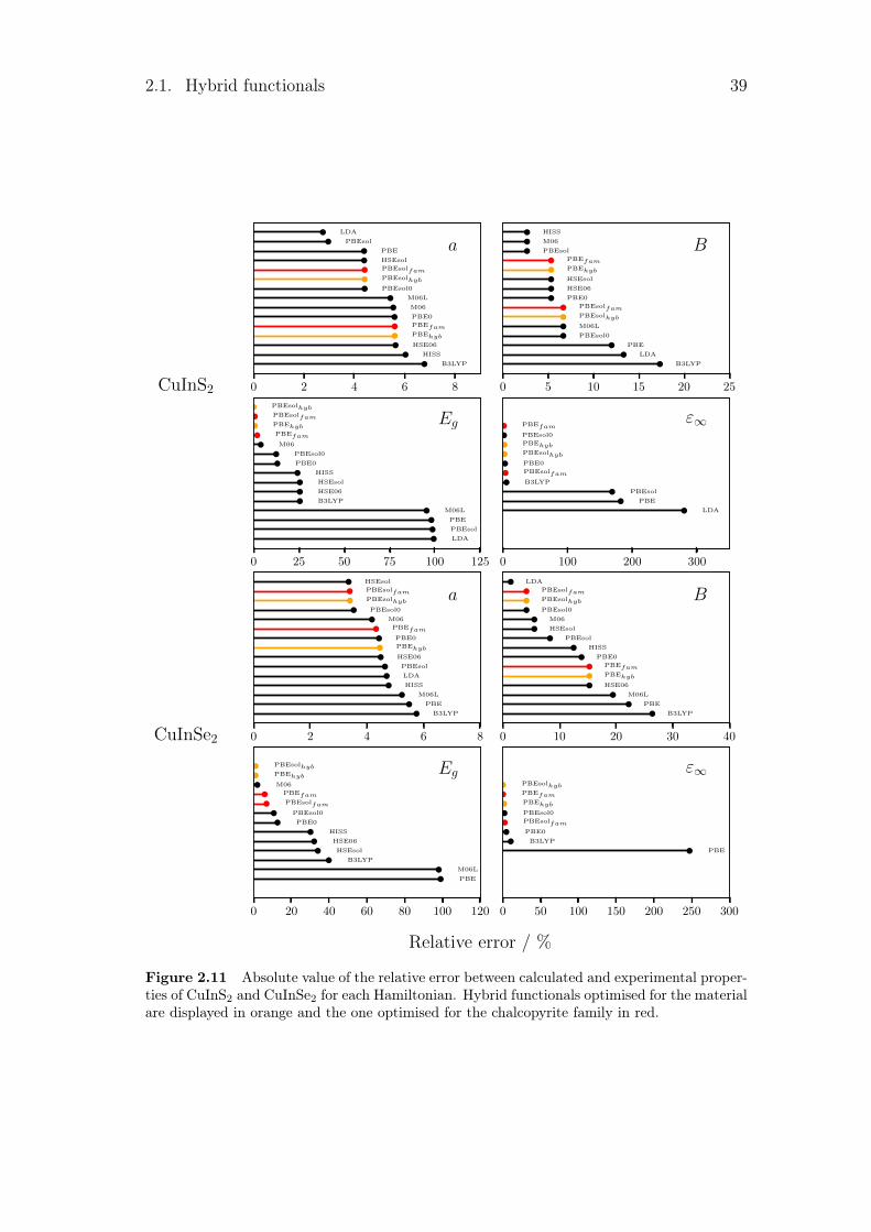
2.1. Hybrid functionals 39
0 2 4 6 8
B3LYP
HISS
HSE06
PBEhyb
PBEfam
PBE0
M06
M06L
PBEsol0
PBEsolhyb
PBEsolfam
HSEsol
PBE
PBEsol
LDA
a
CuInS2 0 5 10 15 20 25
B3LYP
LDA
PBE
PBEsol0
M06L
PBEsolhyb
PBEsolfam
PBE0
HSE06
HSEsol
PBEhyb
PBEfam
PBEsol
M06
HISS
B
0 25 50 75 100 125
LDA
PBEsol
PBE
M06L
B3LYP
HSE06
HSEsol
HISS
PBE0
PBEsol0
M06
PBEfam
PBEhyb
PBEsolfam
PBEsolhyb
Eg
0 100 200 300
LDA
PBE
PBEsol
B3LYP
PBEsolfam
PBE0
PBEsolhyb
PBEhyb
PBEsol0
PBEfamε∞
0 2 4 6 8
B3LYP
PBE
M06L
HISS
LDA
PBEsol
HSE06
PBEhyb
PBE0
PBEfam
M06
PBEsol0
PBEsolhyb
PBEsolfam
HSEsol
a
CuInSe2 0 10 20 30 40
B3LYP
PBE
M06L
HSE06
PBEhyb
PBEfam
PBE0
HISS
PBEsol
HSEsol
M06
PBEsol0
PBEsolhyb
PBEsolfam
LDA
B
0 20 40 60 80 100 120
PBE
M06L
B3LYP
HSEsol
HSE06
HISS
PBE0
PBEsol0
PBEsolfam
PBEfam
M06
PBEhyb
PBEsolhyb Eg
Relative error / %
0 50 100 150 200 250 300
PBE
B3LYP
PBE0
PBEsolfam
PBEsol0
PBEhyb
PBEfam
PBEsolhyb
ε∞
Figure 2.11 Absolute value of the relative error between calculated and experimental proper-ties of CuInS2 and CuInSe2 for each Hamiltonian. Hybrid functionals optimised for the materialare displayed in orange and the one optimised for the chalcopyrite family in red.
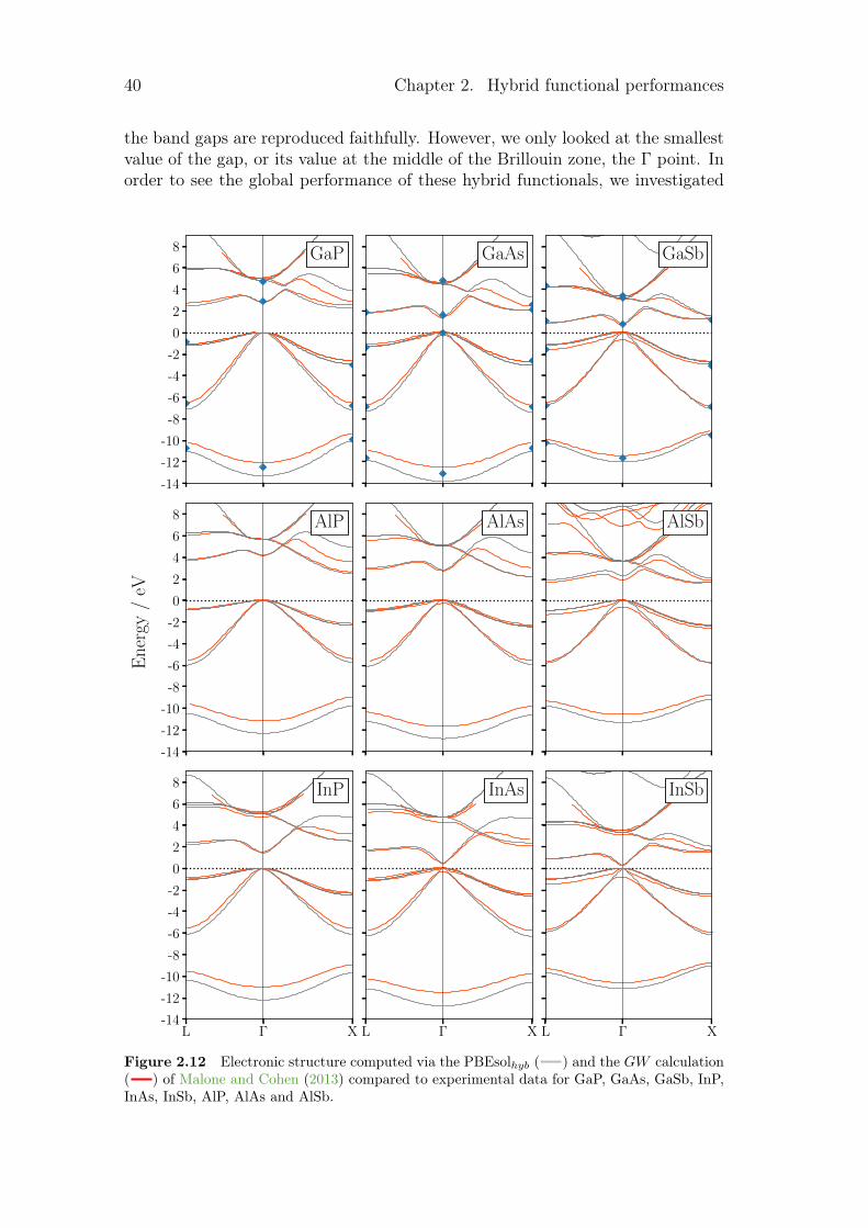
40 Chapter 2. Hybrid functional performances
the band gaps are reproduced faithfully. However, we only looked at the smallestvalue of the gap, or its value at the middle of the Brillouin zone, the Γ point. Inorder to see the global performance of these hybrid functionals, we investigated
-14
-12
-10
-8
-6
-4
-2
0
2
4
6
8 GaP GaAs GaSb
-14
-12
-10
-8
-6
-4
-2
0
2
4
6
8 AlP
En
ergy
/eV
AlAs AlSb
L Γ X-14
-12
-10
-8
-6
-4
-2
0
2
4
6
8 InP
L Γ X
InAs
L Γ X
InSb
Figure 2.12 Electronic structure computed via the PBEsolhyb ( ) and the GW calculation( ) of Malone and Cohen (2013) compared to experimental data for GaP, GaAs, GaSb, InP,InAs, InSb, AlP, AlAs and AlSb.
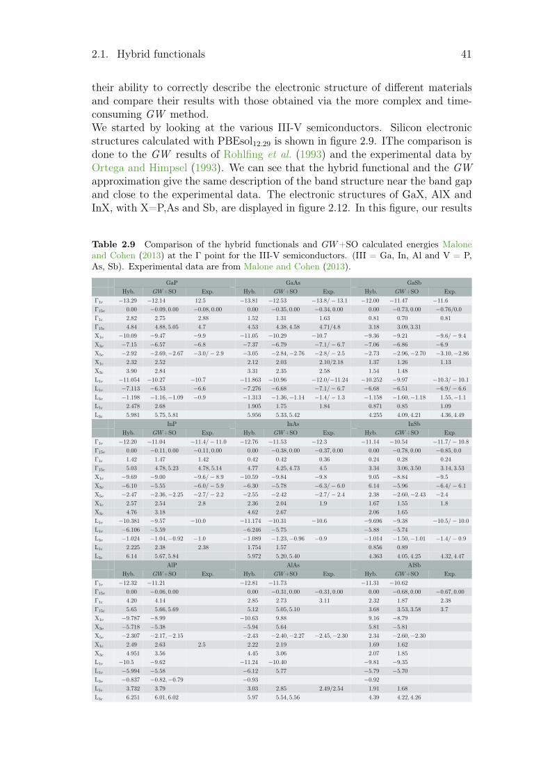
2.1. Hybrid functionals 41
their ability to correctly describe the electronic structure of different materialsand compare their results with those obtained via the more complex and time-consuming GW method.We started by looking at the various III-V semiconductors. Silicon electronicstructures calculated with PBEsol12.29 is shown in figure 2.9. IThe comparison isdone to the GW results of Rohlfing et al. (1993) and the experimental data byOrtega and Himpsel (1993). We can see that the hybrid functional and the GWapproximation give the same description of the band structure near the band gapand close to the experimental data. The electronic structures of GaX, AlX andInX, with X=P,As and Sb, are displayed in figure 2.12. In this figure, our results
Table 2.9 Comparison of the hybrid functionals and GW+SO calculated energies Maloneand Cohen (2013) at the Γ point for the III-V semiconductors. (III = Ga, In, Al and V = P,As, Sb). Experimental data are from Malone and Cohen (2013).
GaP GaAs GaSbHyb. GW+SO Exp. Hyb. GW+SO Exp. Hyb. GW+SO Exp.
Γ1v −13.29 −12.14 12.5 −13.81 −12.53 −13.8/− 13.1 −12.00 −11.47 −11.6
Γ15v 0.00 −0.09, 0.00 −0.08, 0.00 0.00 −0.35, 0.00 −0.34, 0.00 0.00 −0.73, 0.00 −0.76/0.0
Γ1c 2.82 2.75 2.88 1.52 1.31 1.63 0.81 0.70 0.81
Γ15c 4.84 4.88, 5.05 4.7 4.53 4.38, 4.58 4.71/4.8 3.18 3.09, 3.31
X1v −10.09 −9.47 −9.9 −11.05 −10.29 −10.7 −9.36 −9.21 −9.6/− 9.4
X3v −7.15 −6.57 −6.8 −7.37 −6.79 −7.1/− 6.7 −7.06 −6.86 −6.9
X5v −2.92 −2.69,−2.67 −3.0/− 2.9 −3.05 −2.84,−2.76 −2.8/− 2.5 −2.73 −2.96,−2.70 −3.10,−2.86
X1c 2.32 2.52 2.12 2.03 2.10/2.18 1.37 1.26 1.13
X3c 3.90 2.84 3.31 2.35 2.58 1.54 1.48
L1v −11.054 −10.27 −10.7 −11.863 −10.96 −12.0/−11.24 −10.252 −9.97 −10.3/− 10.1
L1v −7.113 −6.53 −6.6 −7.276 −6.68 −7.1/− 6.7 −6.68 −6.51 −6.9/− 6.6
L3v −1.198 −1.16,−1.09 −0.9 −1.313 −1.36,−1.14 −1.4/− 1.3 −1.158 −1.60,−1.18 1.55,−1.1
L1c 2.478 2.68 1.905 1.75 1.84 0.871 0.85 1.09
L3c 5.981 5.75, 5.81 5.956 5.33, 5.42 4.255 4.09, 4.21 4.36, 4.49
InP InAs InSbHyb. GW+SO Exp. Hyb. GW+SO Exp. Hyb. GW+SO Exp.
Γ1v −12.20 −11.04 −11.4/− 11.0 −12.76 −11.53 −12.3 −11.14 −10.54 −11.7/− 10.8
Γ15v 0.00 −0.11, 0.00 −0.11, 0.00 0.00 −0.38, 0.00 −0.37, 0.00 0.00 −0.78, 0.00 −0.85, 0.0
Γ1c 1.42 1.47 1.42 0.42 0.42 0.36 0.24 0.28 0.24
Γ15c 5.03 4.78, 5.23 4.78, 5.14 4.77 4.25, 4.73 4.5 3.34 3.06, 3.50 3.14, 3.53
X1v −9.69 −9.00 −9.6/− 8.9 −10.59 −9.84 −9.8 9.05 −8.84 −9.5
X3v −6.10 −5.55 −6.0/− 5.9 −6.30 −5.78 −6.3/− 6.0 6.14 −5.96 −6.4/− 6.1
X5v −2.47 −2.36,−2.25 −2.7/− 2.2 −2.55 −2.42 −2.7/− 2.4 2.38 −2.60,−2.43 −2.4
X1c 2.57 2.54 2.8 2.36 2.04 1.9 1.67 1.55 1.8
X3c 4.76 3.18 4.62 2.67 2.06 1.65
L1v −10.381 −9.57 −10.0 −11.174 −10.31 −10.6 −9.696 −9.38 −10.5/− 10.0
L1v −6.106 −5.59 −6.246 −5.75 −5.88 −5.74
L3v −1.024 −1.04,−0.92 −1.0 −1.089 −1.23,−0.96 −0.9 −1.014 −1.50,−1.01 −1.4/− 0.9
L1c 2.225 2.38 2.38 1.754 1.57 0.856 0.89
L3c 6.14 5.67, 5.84 5.972 5.20, 5.40 4.363 4.05, 4.25 4.32, 4.47
AlP AlAs AlSbHyb. GW+SO Exp. Hyb. GW+SO Exp. Hyb. GW+SO Exp.
Γ1v −12.32 −11.21 −12.81 −11.73 −11.31 −10.62
Γ15v 0.00 −0.06, 0.00 0.00 −0.31, 0.00 −0.31, 0.00 0.00 −0.68, 0.00 −0.67, 0.00
Γ1c 4.20 4.14 2.85 2.73 3.11 2.32 1.87 2.38
Γ15c 5.65 5.66, 5.69 5.12 5.05, 5.10 3.68 3.53, 3.58 3.7
X1v −9.787 −8.99 −10.63 9.88 9.16 −8.79
X3v −5.718 −5.38 −5.94 5.64 5.81 −5.81
X5v −2.307 −2.17,−2.15 −2.43 −2.40,−2.27 −2.45,−2.30 2.34 −2.60,−2.30
X1c 2.49 2.63 2.5 2.22 2.19 1.69 1.62
X3c 4.951 3.56 4.45 3.06 2.07 1.85
L1v −10.5 −9.62 −11.24 −10.40 −9.81 −9.35
L1v −5.994 −5.58 −6.12 5.77 −5.79 −5.70
L3v −0.837 −0.82,−0.79 −0.93 −0.92
L1c 3.732 3.79 3.03 2.85 2.49/2.54 1.91 1.68
L3c 6.251 6.01, 6.02 5.97 5.54, 5.56 4.39 4.22, 4.26
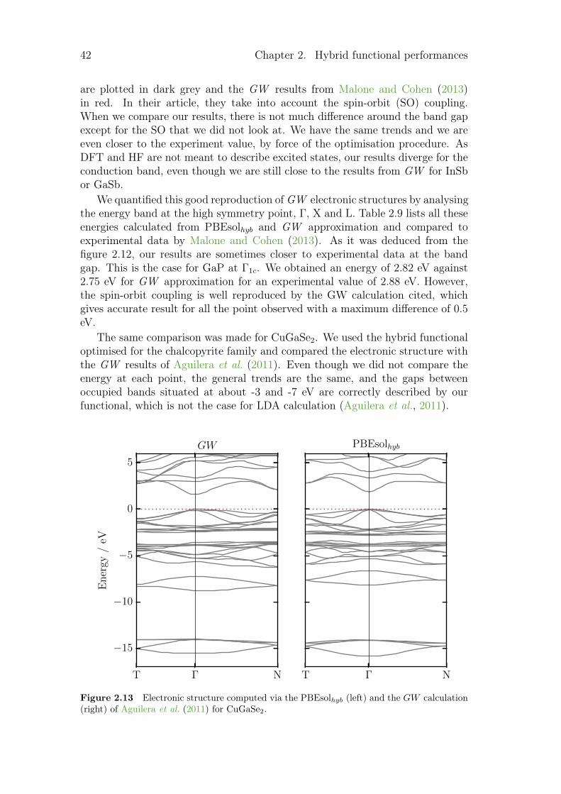
42 Chapter 2. Hybrid functional performances
are plotted in dark grey and the GW results from Malone and Cohen (2013)in red. In their article, they take into account the spin-orbit (SO) coupling.When we compare our results, there is not much difference around the band gapexcept for the SO that we did not look at. We have the same trends and we areeven closer to the experiment value, by force of the optimisation procedure. AsDFT and HF are not meant to describe excited states, our results diverge for theconduction band, even though we are still close to the results from GW for InSbor GaSb.
We quantified this good reproduction ofGW electronic structures by analysingthe energy band at the high symmetry point, Γ, X and L. Table 2.9 lists all theseenergies calculated from PBEsolhyb and GW approximation and compared toexperimental data by Malone and Cohen (2013). As it was deduced from thefigure 2.12, our results are sometimes closer to experimental data at the bandgap. This is the case for GaP at Γ1c. We obtained an energy of 2.82 eV against2.75 eV for GW approximation for an experimental value of 2.88 eV. However,the spin-orbit coupling is well reproduced by the GW calculation cited, whichgives accurate result for all the point observed with a maximum difference of 0.5eV.
The same comparison was made for CuGaSe2. We used the hybrid functionaloptimised for the chalcopyrite family and compared the electronic structure withthe GW results of Aguilera et al. (2011). Even though we did not compare theenergy at each point, the general trends are the same, and the gaps betweenoccupied bands situated at about -3 and -7 eV are correctly described by ourfunctional, which is not the case for LDA calculation (Aguilera et al., 2011).
T Γ N
GW
−15
−10
−5
0
5
En
ergy
/eV
T Γ N
PBEsolhyb
Figure 2.13 Electronic structure computed via the PBEsolhyb (left) and the GW calculation(right) of Aguilera et al. (2011) for CuGaSe2.

2.2. Temperature dependence of various properties 43
Hence, the accuracy of the hybrid functional is remarkably close to the one ob-tained with most complex method as GW approximation. We developed hybridfunctional that has the same precision on structural, mechanical and vibrationalproperties of other functionals in the literature, a better description of the di-electric properties and enables a very accurate reproduction of the band gap andof the electronic structure as a whole. Far less ressources-consuming than GWmethods, our hybrid Hamiltonian are thus a pragmatic way to obtain quick andaccurate result for semiconductors used in the photovoltaic field.
2.2 Temperature dependence of various proper-ties
2.2.1 Structural parameters
In QHA, the effect of the temperature is directly linked to the thermal evolutionof the lattice structure. Each temperature corresponds to a specific set of latticeconstants. This is why the first type of properties to consider when looking atthe QHA is the structural parameters and/or thermal expansion coefficient.
Figure 2.14 represents the variation of the thermal expansion coefficient α withthe temperature for the set of semiconductors studied in this thesis for differentHamiltonians. These computed variations were compared to experimental datafrom literature. The behaviour of the calculated thermal expansion coefficientis close to the experimental ones for all the materials of figure 2.14. The onlydivergence is an underestimation for several III-V semiconductors (AlP, AlAs,AlSb and GaSb). We can see that we have a good description of the negativethermal expansion at low temperatures. It has been observed for various III-Vsemiconductors and Si and is due to the negative Grüneissen parameters of thetransverse acoustical phonon branches near the limit of the Brillouin zone (Somaet al., 1982; Sparks and Swenson, 1967; Gibbons, 1958; Xu et al., 1991; Biernackiand Scheffler, 1989). The QHA successfully reproduces this behaviour and evenhas a small tendency to overestimate it as it can be seen for the Al- and In-basedIII-V semiconductors. The comparison of the different functionals shows similarbehaviour and small dispersion. The highest difference between two functionalsat a fixed temperature does not exceed 3 × 10⁻⁶ K−1 and is only obtained forgermanium which exhibits the maximum dispersion.
We then looked at the lattice expansion of copper-based ternary chalcopy-rites. In this case, the anisotropy of the system leads to two different thermalexpansion coefficients αa and αc. Figure 2.15 shows their variation with the tem-perature. The Hamiltonian used is the PBEsol-based optimised one for the wholechalcopyrite family (see section 2.1.1). The above observation, concerning a goodreproduction of the experimental data, applies in this case as well. However, thedifference between αa and αc is smaller when calculated than according to exper-iment. This is particularly true for CuGaSe2 where the two calculated curves arenearly overlapping. For this material, the negative thermal expansion is not well
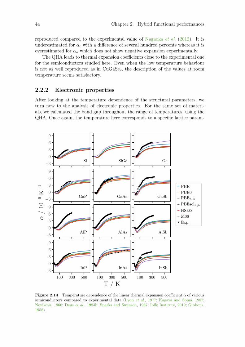
44 Chapter 2. Hybrid functional performances
reproduced compared to the experimental value of Nagaoka et al. (2012). It isunderestimated for αc with a difference of several hundred percents whereas it isoverestimated for αa which does not show negative expansion experimentally.
The QHA leads to thermal expansion coefficients close to the experimental onefor the semiconductors studied here. Even when the low temperature behaviouris not as well reproduced as in CuGaSe2, the description of the values at roomtemperature seems satisfactory.
2.2.2 Electronic properties
After looking at the temperature dependence of the structural parameters, weturn now to the analysis of electronic properties. For the same set of materi-als, we calculated the band gap throughout the range of temperatures, using theQHA. Once again, the temperature here corresponds to a specific lattice param-
−3
0
3
6
9
Si SiGe Ge
−3
0
3
6
9
GaP GaAs GaSb
−3
0
3
6
9
AlP
α/
10−
6·K−
1
AlAs AlSb
PBE
PBE0
PBEhyb
PBEsolhyb
HSE06
M06
Exp.
100 300 500
−3
0
3
6
9
InP
100 300 500
InAs
T / K100 300 500
InSb
Figure 2.14 Temperature dependence of the linear thermal expansion coefficient α of varioussemiconductors compared to experimental data (Lyon et al., 1977; Kagaya and Soma, 1987;Novikova, 1966; Deus et al., 1983b; Sparks and Swenson, 1967; Ioffe Institute, 2019; Gibbons,1958).
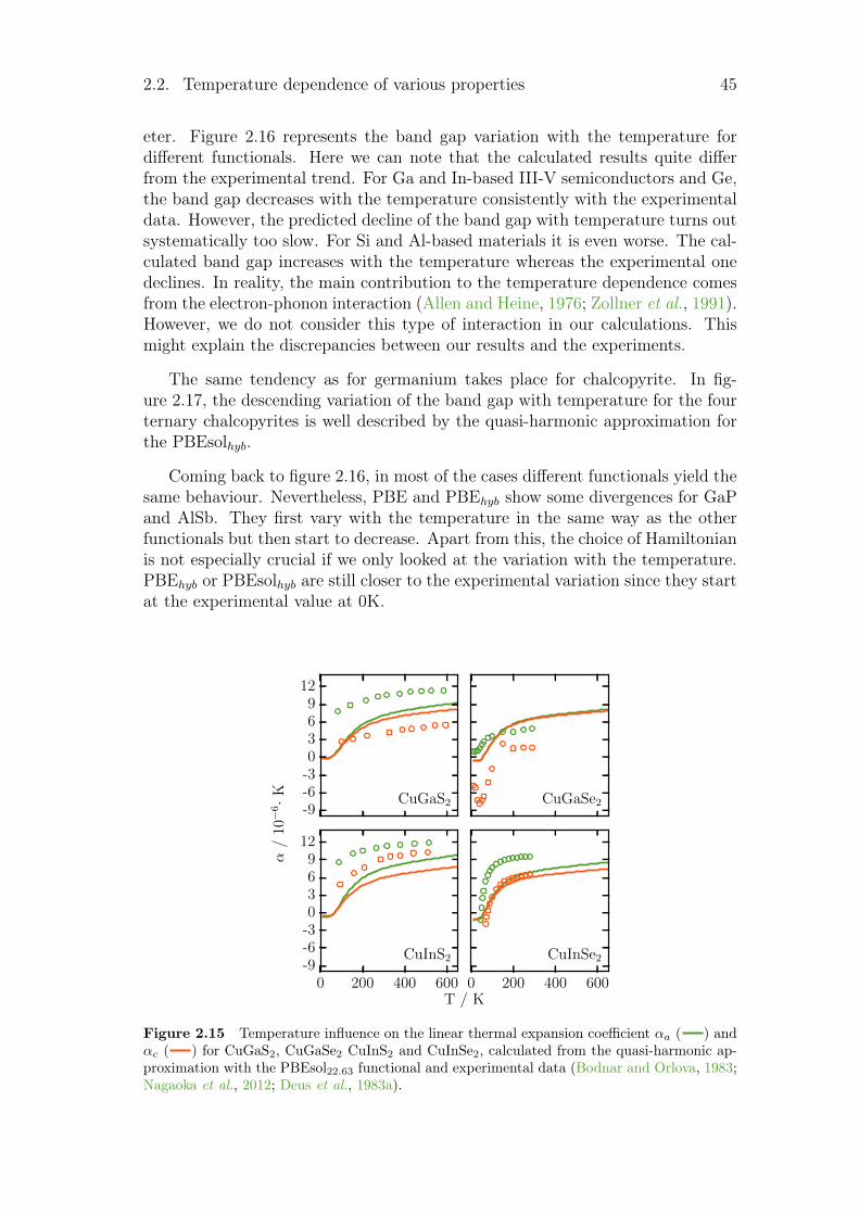
2.2. Temperature dependence of various properties 45
eter. Figure 2.16 represents the band gap variation with the temperature fordifferent functionals. Here we can note that the calculated results quite differfrom the experimental trend. For Ga and In-based III-V semiconductors and Ge,the band gap decreases with the temperature consistently with the experimentaldata. However, the predicted decline of the band gap with temperature turns outsystematically too slow. For Si and Al-based materials it is even worse. The cal-culated band gap increases with the temperature whereas the experimental onedeclines. In reality, the main contribution to the temperature dependence comesfrom the electron-phonon interaction (Allen and Heine, 1976; Zollner et al., 1991).However, we do not consider this type of interaction in our calculations. Thismight explain the discrepancies between our results and the experiments.
The same tendency as for germanium takes place for chalcopyrite. In fig-ure 2.17, the descending variation of the band gap with temperature for the fourternary chalcopyrites is well described by the quasi-harmonic approximation forthe PBEsolhyb.
Coming back to figure 2.16, in most of the cases different functionals yield thesame behaviour. Nevertheless, PBE and PBEhyb show some divergences for GaPand AlSb. They first vary with the temperature in the same way as the otherfunctionals but then start to decrease. Apart from this, the choice of Hamiltonianis not especially crucial if we only looked at the variation with the temperature.PBEhyb or PBEsolhyb are still closer to the experimental variation since they startat the experimental value at 0K.
-9-6-30369
12
α/
10−
6·K CuGaS2 CuGaSe2
0 200 400 600-9-6-30369
12
T / K
CuInS2
0 200 400 600
CuInSe2
Figure 2.15 Temperature influence on the linear thermal expansion coefficient αa ( ) andαc ( ) for CuGaS2, CuGaSe2 CuInS2 and CuInSe2, calculated from the quasi-harmonic ap-proximation with the PBEsol22.63 functional and experimental data (Bodnar and Orlova, 1983;Nagaoka et al., 2012; Deus et al., 1983a).
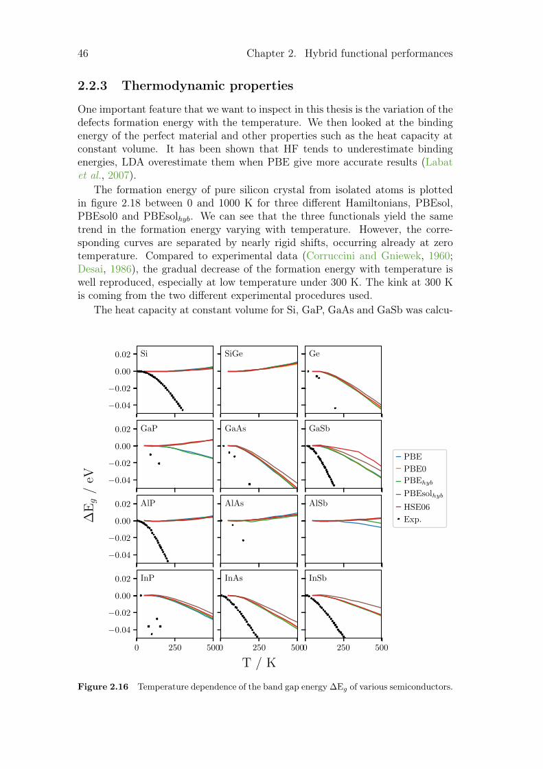
46 Chapter 2. Hybrid functional performances
2.2.3 Thermodynamic properties
One important feature that we want to inspect in this thesis is the variation of thedefects formation energy with the temperature. We then looked at the bindingenergy of the perfect material and other properties such as the heat capacity atconstant volume. It has been shown that HF tends to underestimate bindingenergies, LDA overestimate them when PBE give more accurate results (Labatet al., 2007).
The formation energy of pure silicon crystal from isolated atoms is plottedin figure 2.18 between 0 and 1000 K for three different Hamiltonians, PBEsol,PBEsol0 and PBEsolhyb. We can see that the three functionals yield the sametrend in the formation energy varying with temperature. However, the corre-sponding curves are separated by nearly rigid shifts, occurring already at zerotemperature. Compared to experimental data (Corruccini and Gniewek, 1960;Desai, 1986), the gradual decrease of the formation energy with temperature iswell reproduced, especially at low temperature under 300 K. The kink at 300 Kis coming from the two different experimental procedures used.
The heat capacity at constant volume for Si, GaP, GaAs and GaSb was calcu-
−0.04
−0.02
0.00
0.02 Si SiGe Ge
−0.04
−0.02
0.00
0.02 GaP GaAs GaSb
PBE
PBE0
PBEhyb
PBEsolhyb
HSE06
Exp.
−0.04
−0.02
0.00
0.02 AlP
∆Eg
/eV
AlAs AlSb
0 250 500
−0.04
−0.02
0.00
0.02 InP
0 250 500
InAs
T / K
0 250 500
InSb
Figure 2.16 Temperature dependence of the band gap energy ∆Eg of various semiconductors.
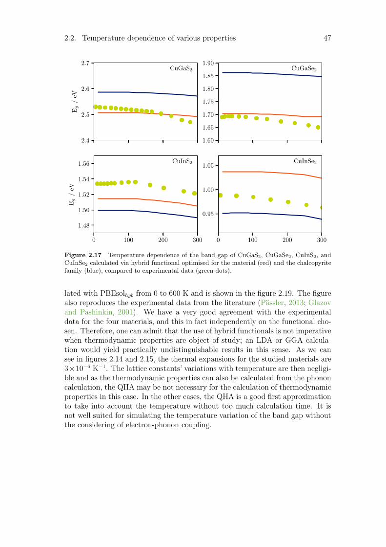
2.2. Temperature dependence of various properties 47
2.4
2.5
2.6
2.7
Eg
/eV
CuGaS2
1.60
1.65
1.70
1.75
1.80
1.85
1.90CuGaSe2
0 100 200 300
1.48
1.50
1.52
1.54
1.56
Eg
/eV
CuInS2
0 100 200 300
0.95
1.00
1.05CuInSe2
Figure 2.17 Temperature dependence of the band gap of CuGaS2, CuGaSe2, CuInS2, andCuInSe2 calculated via hybrid functional optimised for the material (red) and the chalcopyritefamily (blue), compared to experimental data (green dots).
lated with PBEsolhyb from 0 to 600 K and is shown in the figure 2.19. The figurealso reproduces the experimental data from the literature (Pässler, 2013; Glazovand Pashinkin, 2001). We have a very good agreement with the experimentaldata for the four materials, and this in fact independently on the functional cho-sen. Therefore, one can admit that the use of hybrid functionals is not imperativewhen thermodynamic properties are object of study; an LDA or GGA calcula-tion would yield practically undistinguishable results in this sense. As we cansee in figures 2.14 and 2.15, the thermal expansions for the studied materials are3×10−6 K−1. The lattice constants’ variations with temperature are then negligi-ble and as the thermodynamic properties can also be calculated from the phononcalculation, the QHA may be not necessary for the calculation of thermodynamicproperties in this case. In the other cases, the QHA is a good first approximationto take into account the temperature without too much calculation time. It isnot well suited for simulating the temperature variation of the band gap withoutthe considering of electron-phonon coupling.

48 Chapter 2. Hybrid functional performances
0 200 400 600 800 1000
T / K
−560
−540
−520
−500
−480
−460
−440
−420
Eformation
/kJ.m
ol−
1.K−
1PBEsol
PBEsol0
PBEsolhyb
Figure 2.18 Formation energy of silicon for three different Hamiltonians compared to exper-imental data from Corruccini and Gniewek (1960) (•) and Desai (1986) (•).
0 100 200 300 400 500 600
T / K
0
10
20
30
40
50
60
Hea
tC
apaci
ty/
J·K−
1·m
ol−
1
Si
GaP
GaAs
GaSb
Figure 2.19 Temperature dependence of the heat capacity of Si and GaX (X = P, As andSb) calculated with the PBEsolhyb compared to experimental data (Pässler, 2013; Glazov andPashinkin, 2001).

2.3. Electrical conductivity 49
2.3 Electrical conductivity
The last type of properties than we want to reach in this thesis are the transportproperties, especially the electrical conductivity σ. This can be done from theBoltzmann transport equation (BTE). We saw in section 1.4 that there is a lot ofdifferent implementation of the BTE in the literature. Here we used BoltzTraP2.
Effect of the choice of functional
We first investigated the impact of the Hamiltonians on the electrical conduc-tivity. Figure 2.20 shows the variation of the electrical conductivity, normalisedby the relaxation time, with the chemical potential of silicon for different func-tionals. As it has been observed by Sansone et al. (2017), the influence of theHamiltonian is not very important. The trends obtained in calculations usingdifferent hybrid Hamiltonians turn out to be very similar. The curves are prac-tically the same, up to a rigid shift. However, the quantitative analysis showsvariation between functionals. The lower the calculated band gap, the lower theelectrical conductivity. HF has the highest electrical conductivity when PBE hasthe lowest. The only important aspect is the value of the band gap calculatedby the functional. When defects come into play, the chemical potential movesfrom its value at 0 K, the Fermi level. We then need to have the most accuratedescription of the variation of the transport properties near the band gap. This iswhy the self-consistent hybrid functionals developed in this thesis are important.The accurate description of the band gap leads to the most accurate descriptionof the electrical conductivity via the BTE.
−15 −10 −5 0 5 10 15
µ / eV
0
2
4
6
8
10
σ·τ−
1/
1021Ω−
1·m−
1·s−
1
HF
PBE
PBE0
HSE06
PBEhyb
PBEsolhyb
Figure 2.20 Electrical conductivity of silicon calculated with different functionals.

50 Chapter 2. Hybrid functional performances
Effect of the temperature
The quantitative estimation of the electrical conductivity must be done at giventemperature and chemical potential. The influence of temperature is shown infigure 2.21 for silicon for the PBEsol12.29. In this case, the conductivity decreaseswith the temperature. Each system has a particular chemical potential, thatdepends on the doping. For each temperature, it is the one that yields zero netcharge carrier density. For silicon, its variation is only 10−4 eV for 500 K. Wecan then consider that this value is constant with the temperature and take thechemical potential equal to the Fermi level.
Applications
We can then compare the different semiconductor materials. The electrical con-ductivity versus the chemical potential, normalised by the relaxation time, ofdifferent semiconductors is plotted in figure 2.22. Each material has a specificcurve even though the behaviour are usually the same. The electrical conduc-tivity is lower in the valence band compared to the one of the conduction band.The distribution of the electrical conductivity σ is directly linked to the densityof state of the material. Even without looking at the quantitative data, we seethat the normalisation of the electrical conductivity permits to compare materialsbehaviours.
−15 −10 −5 0 5 10 15
µ / eV
0.0
2.5
5.0
7.5
10.0
12.5
15.0
17.5
20.0
σ·τ−
1/
1021Ω−
1·m−
1·s−
1
100
200
300
400
500
600
700
800
Figure 2.21 Temperature dependence of the electrical conductivity of silicon.
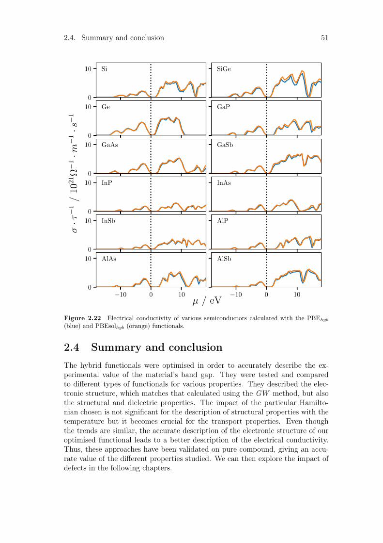
2.4. Summary and conclusion 51
0
10 Si SiGe
0
10 Ge GaP
0
10 GaAs
σ·τ−
1/
1021Ω−
1·m−
1·s−
1
GaSb
0
10 InP InAs
0
10 InSb AlP
−10 0 100
10 AlAs
µ / eV−10 0 10
AlSb
Figure 2.22 Electrical conductivity of various semiconductors calculated with the PBEhyb
(blue) and PBEsolhyb (orange) functionals.
2.4 Summary and conclusionThe hybrid functionals were optimised in order to accurately describe the ex-perimental value of the material’s band gap. They were tested and comparedto different types of functionals for various properties. They described the elec-tronic structure, which matches that calculated using the GW method, but alsothe structural and dielectric properties. The impact of the particular Hamilto-nian chosen is not significant for the description of structural properties with thetemperature but it becomes crucial for the transport properties. Even thoughthe trends are similar, the accurate description of the electronic structure of ouroptimised functional leads to a better description of the electrical conductivity.Thus, these approaches have been validated on pure compound, giving an accu-rate value of the different properties studied. We can then explore the impact ofdefects in the following chapters.


Chapter 3
Chalcopyrite-type compounds fortandem applications
In the previous chapters, the methodology relevant for this thesis was outlinedin what regards theory foundations and practical implementation. Experimentaldata concerning perfect semiconductors were discussed. In the present chapter,this methodology is applied to investigate the chalcopyrite-type complex systemsfor tandem application. In order to use the chalcopyrite as the top cell for a siliconbottom cell, its optimal band gap must be in the range 1.5−1.7 eV. Moreover, thelattice mismatch with the silicon substrate needs to be as small as possible in orderto avoid the growth of a buffer layer. In the following, two types of chalcopyrite-type compounds will be examined. We start by investigating the variation ofconcentrations x and y in CuGaxIn1−xSySe1−y compounds and its impact on thevarious properties of the material. We will then look at the cation (especiallycopper) substitution by alkali metals in four different ternary chalcopyrites.
3.1 Doping/defect incorporation method
Some general remarks on the chalcopyrite structure might be in place here. Thechalcopyrite structure can be viewed as that of II-VI zincblende in which theanions are tetrahedrally coordinated by cations. They have a tetragonal bodycentered Bravais lattice. Their conventional unit cell is shown in the Figure3.1 with 16 atoms (two primitive cells). Their space group is I 42d, and theirstructure is fully described by three crystallographic parameters: the two latticeparameters a, c and the anions fractional coordinate u. The Cu atom is alwaysat the origin, (Ga/In) and (S/Se) atoms at the (0.5, 0.5, 0) and (u, 0.25, 0.125)positions, respectively. As shown in the Figure 3.1, the anions tetrahedra can bedescribed by three internal parameters: d defined as the cation-anion distance, θ1
as the (S/Se) – (Cu/Ga/In) – (S/Se) angle between atoms along the tetrahedra’sbasal plane, and, θ2 as the (S/Se) – (Cu/Ga/In) – (S/Se) angle along the medianof the tetrahedra.
In order to incorporate defect in the bulk material, or to tune its intrinsiccomposition, a procedure is adopted as outlined in figure 3.2. First of all, the
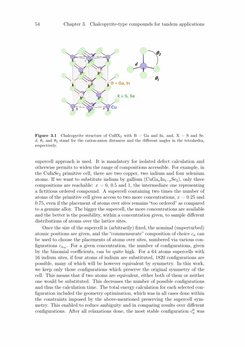
54 Chapter 3. Chalcopyrite-type compounds for tandem applications
d
q1
q2
Figure 3.1 Chalcopyrite structure of CuBX2 with B = Ga and In, and, X = S and Se.d, θ1 and θ2 stand for the cation-anion distances and the different angles in the tetrahedra,respectively.
supercell approach is used. It is mandatory for isolated defect calculation andotherwise permits to widen the range of compositions accessible. For example, inthe CuInSe2 primitive cell, there are two copper, two indium and four seleniumatoms. If we want to substitute indium by gallium (CuGaxIn1−xSe2), only threecompositions are reachable: x = 0, 0.5 and 1, the intermediate one representinga fictitious ordered compound. A supercell containing two times the number ofatoms of the primitive cell gives access to two more concentrations, x = 0.25 and0.75, even if the placement of atoms over sites remains “too ordered” as comparedto a genuine alloy. The bigger the supercell, the more concentrations are availableand the better is the possibility, within a concentration given, to sample differentdistributions of atoms over the lattice sites.
Once the size of the supercell is (arbitrarily) fixed, the nominal (unperturbed)atomic positions are given, and the “commensurate” composition of choice cn canbe used to choose the placements of atoms over sites, numbered via various con-figurations cnm . For a given concentration, the number of configurations, givenby the binomial coefficients, can be quite high. For a 64 atoms supercells with16 indium sites, if four atoms of indium are substituted, 1820 configurations arepossible, many of which will be however equivalent by symmetry. In this work,we keep only those configurations which preserve the original symmetry of thecell. This means that if two atoms are equivalent, either both of them or neitherone would be substituted. This decreases the number of possible configurationsand thus the calculation time. The total energy calculation for each selected con-figuration included the geometry optimisation, which was in all cases done withinthe constraints imposed by the above-mentioned preserving the supercell sym-metry. This enabled to reduce ambiguity and in comparing results over differentconfigurations. After all relaxations done, the most stable configuration c0
n was
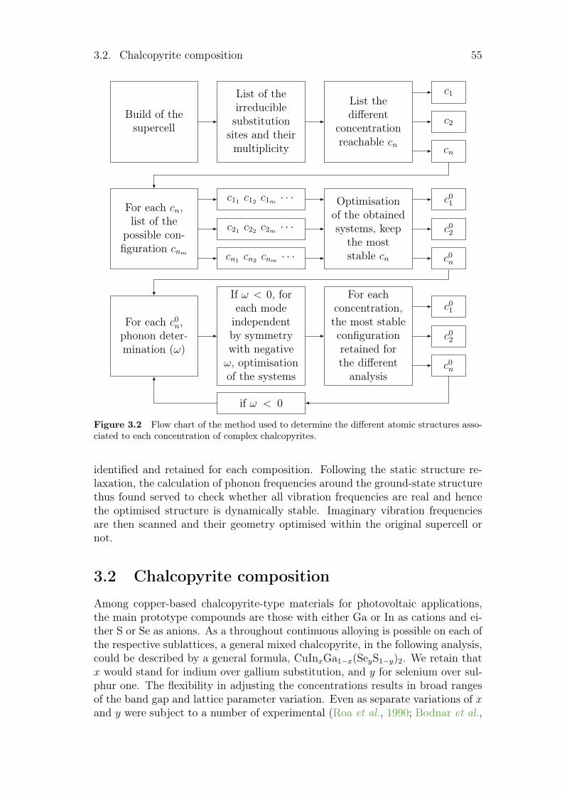
3.2. Chalcopyrite composition 55
Build of thesupercell
List of theirreduciblesubstitution
sites and theirmultiplicity
List thedifferent
concentrationreachable cn
c1
c2
cn
For each cn,list of the
possible con-figuration cnm
c11 c12 c1m · · ·
c21 c22 c2m · · ·
cn1 cn2 cnm · · ·
Optimisationof the obtainedsystems, keep
the moststable cn
c01
c02
c0n
For each c0n,
phonon deter-mination (ω)
If ω < 0, foreach modeindependentby symmetrywith negativeω, optimisationof the systems
For eachconcentration,the most stableconfigurationretained forthe differentanalysis
c01
c02
c0n
if ω < 0
Figure 3.2 Flow chart of the method used to determine the different atomic structures asso-ciated to each concentration of complex chalcopyrites.
identified and retained for each composition. Following the static structure re-laxation, the calculation of phonon frequencies around the ground-state structurethus found served to check whether all vibration frequencies are real and hencethe optimised structure is dynamically stable. Imaginary vibration frequenciesare then scanned and their geometry optimised within the original supercell ornot.
3.2 Chalcopyrite composition
Among copper-based chalcopyrite-type materials for photovoltaic applications,the main prototype compounds are those with either Ga or In as cations and ei-ther S or Se as anions. As a throughout continuous alloying is possible on each ofthe respective sublattices, a general mixed chalcopyrite, in the following analysis,could be described by a general formula, CuInxGa1−x(SeyS1−y)2. We retain thatx would stand for indium over gallium substitution, and y for selenium over sul-phur one. The flexibility in adjusting the concentrations results in broad rangesof the band gap and lattice parameter variation. Even as separate variations of xand y were subject to a number of experimental (Roa et al., 1990; Bodnar et al.,
56 Chapter 3. Chalcopyrite-type compounds for tandem applications
1981; Bodnar and Lukomskii, 1986; Tinoco et al., 1991) and theoretical (Jiangand Feng, 2008) studies, only one work, to our knowledge, addressed both sub-stitutions simultaneously (Bär et al., 2004). In this work, a model was proposedto parametrise the band gap of CuInxGa1−x(SeyS1−y)2, by extending the usualdescription of the band gap in binary compounds A1−xBx:
Eg(x) = (1− x)Eg(A) + xEg(B)− bx(1− x) , (3.1)
where b is the optical bowing constant Wei and Zunger (1995). For the penternarychalcopyrite, Bär et al. (2004) obtained the following band gap (in eV):
Eg(x, y) = 1.00 + 0.13x2 + 0.08y2 + 0.13xy + 0.55x+ 0.54y. (3.2)
In the present study, the band gap was probed in a series of first-principles calcu-lations on a number of mixed structures. In particular, 81 different compositionsfor CuInxGa1−x(SeyS1−y)2 were analysed via the procedure described in figure 3.2.This 81-sample mesh corresponds to 9×9 trials with the values of 0, 1
8, 2
8, . . . , 7
8, 1
over both x and y. As some concentrations could have been represented by manydifferent configurations of atoms within the given supercell size and composition,the geometry optimisations have been performed on more than eight hundredsconfigurations, in order to identify the most competitive ones. In all cases, thetrial systems maintained the symmetry of the chalcopyrite space group. Thestructural, electronic and thermodynamic properties of these compounds werethen analysed under an angle of identifying the range of composition suited fortandem application.
3.2.1 The variation of the band gap with concentration
The effect of concentration on the band gap in mixed chalcopyrite-type com-pounds is shown at the top of figure 3.3. The four corner points of the figureare occupied by the perfect ternary compounds CuGaS2, CuGaSe2, CuInS2 andCuInSe2. The variation of the band gap is linear with both the concentration ofIn x and Se y, just as it was reported in the work of Bär et al. (2004). For a varia-tion of x or y of 10 %, the increase of gap throughout x is ∼1 eV but throughout yonly ∼0.6 eV. The whole span of the band gap variation across the diagonal of theplot goes from 1.03 eV for CuInSe2 to 2.53 eV for CuGaS2. Separately, both thegallium and sulphur incorporation increase the band gap value. The interestingrange of 1.5-1.7 eV for tandem cells is well defined in the figure. It correspondsto the parallelepiped delimited by (x, y) = (0.2, 1); (0.4, 1); (0.8, 0); (1, 1).
Whereas the inner region of this (x, y) map was not systematically investigatedexperimentally, the works have been done accurately exploring its four borders.A comparison of our calculations with these data are shown in figure 3.4. A verygood agreement is found for all binary trends, especially for CuIn(Se2S1−x)2. Animportant conclusion from this is that our optimised hybrid functional is quiteaccurate throughout the whole range of substitutions and is then a reasonablecompromise to use for practical predictions of electronic structure concerningthis family of compounds. This conclusion gets further support from the resultsconcerning the lattice parameters, reported in the following section.
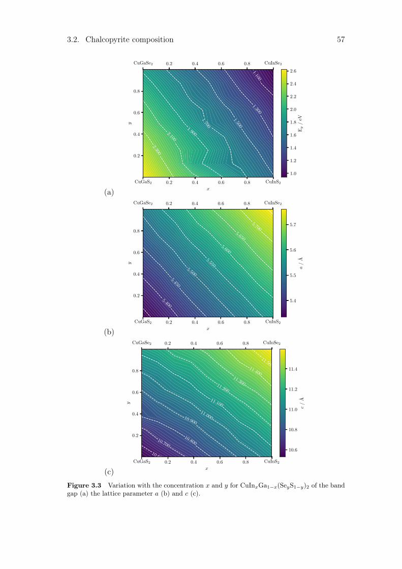
3.2. Chalcopyrite composition 57
(a)CuGaS2 0.2 0.4 0.6 0.8 CuInS2
x
0.2
0.4
0.6
0.8
y
1.1001.300
1.500
1.700
1.9002.100
2.300
CuGaSe2 0.2 0.4 0.6 0.8 CuInSe2
1.0
1.2
1.4
1.6
1.8
2.0
2.2
2.4
2.6
Eg
/eV
(b)CuGaS2 0.2 0.4 0.6 0.8 CuInS2
x
0.2
0.4
0.6
0.8
y
5.400
5.450
5.500
5.550
5.600
5.650
5.700
CuGaSe2 0.2 0.4 0.6 0.8 CuInSe2
5.4
5.5
5.6
5.7
a/
A
(c)CuGaS2 0.2 0.4 0.6 0.8 CuInS2
x
0.2
0.4
0.6
0.8
y
10.600
10.700
10.800
10.900
11.000
11.100
11.200
11.300
11.400
11.500
CuGaSe2 0.2 0.4 0.6 0.8 CuInSe2
10.6
10.8
11.0
11.2
11.4
c/
A
Figure 3.3 Variation with the concentration x and y for CuInxGa1−x(SeyS1−y)2 of the bandgap (a) the lattice parameter a (b) and c (c).
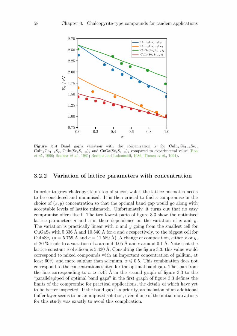
58 Chapter 3. Chalcopyrite-type compounds for tandem applications
0.0 0.2 0.4 0.6 0.8 1.0
x
0.75
1.00
1.25
1.50
1.75
2.00
2.25
2.50
2.75
Eg
/eV
CuInxGa1−xS2
CuInxGa1−xSe2
CuGa(SexS1−x)2
CuIn(SexS1−x)2
Figure 3.4 Band gap’s variation with the concentration x for CuInxGa1−xSe2,CuInxGa1−xS2, CuIn(SexS1−x)2 and CuGa(SexS1−x)2 compared to experimental value (Roaet al., 1990; Bodnar et al., 1981; Bodnar and Lukomskii, 1986; Tinoco et al., 1991).
3.2.2 Variation of lattice parameters with concentration
In order to grow chalcopyrite on top of silicon wafer, the lattice mismatch needsto be considered and minimised. It is then crucial to find a compromise in thechoice of (x, y) concentration so that the optimal band gap would go along withacceptable levels of lattice mismatch. Unfortunately, it turns out that no easycompromise offers itself. The two lowest parts of figure 3.3 show the optimisedlattice parameters a and c in their dependence on the variation of x and y.The variation is practically linear with x and y going from the smallest cell forCuGaS2 with 5.336 Å and 10.540 Å for a and c respectively, to the biggest cell forCuInSe2 (a = 5.759 Å and c = 11.589 Å). A change of composition, either x or y,of 20 % leads to a variation of a around 0.05 Å and c around 0.1 Å. Note that thelattice constant a of silicon is 5.430 Å. Consulting the figure 3.3, this value wouldcorrespond to mixed compounds with an important concentration of gallium, atleast 60%, and more sulphur than selenium, x 6 0.5. This combination does notcorrespond to the concentrations suited for the optimal band gap. The span fromthe line corresponding to a ' 5.43 Å in the second graph of figure 3.3 to the“parallelepiped of optimal band gaps” in the first graph of figure 3.3 defines thelimits of the compromise for practical applications, the details of which have yetto be better inspected. If the band gap is a priority, an inclusion of an additionalbuffer layer seems to be an imposed solution, even if one of the initial motivationsfor this study was exactly to avoid this complication.
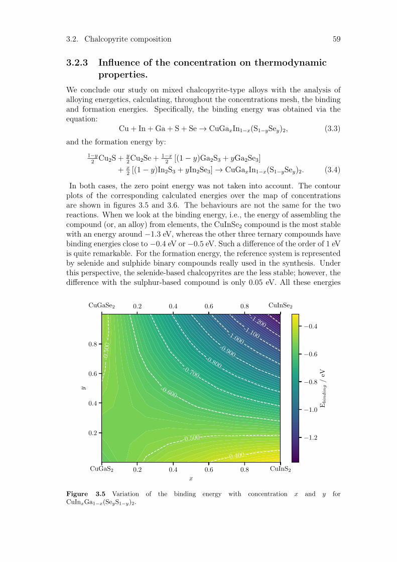
3.2. Chalcopyrite composition 59
3.2.3 Influence of the concentration on thermodynamicproperties.
We conclude our study on mixed chalcopyrite-type alloys with the analysis ofalloying energetics, calculating, throughout the concentrations mesh, the bindingand formation energies. Specifically, the binding energy was obtained via theequation:
Cu + In + Ga + S + Se→ CuGaxIn1−x(S1−ySey)2, (3.3)
and the formation energy by:
1−y2Cu2S + y
2Cu2Se + 1−x
2[(1− y)Ga2S3 + yGa2Se3]
+ x2
[(1− y)In2S3 + yIn2Se3]→ CuGaxIn1−x(S1−ySey)2. (3.4)
In both cases, the zero point energy was not taken into account. The contourplots of the corresponding calculated energies over the map of concentrationsare shown in figures 3.5 and 3.6. The behaviours are not the same for the tworeactions. When we look at the binding energy, i.e., the energy of assembling thecompound (or, an alloy) from elements, the CuInSe2 compound is the most stablewith an energy around −1.3 eV, whereas the other three ternary compounds havebinding energies close to −0.4 eV or −0.5 eV. Such a difference of the order of 1 eVis quite remarkable. For the formation energy, the reference system is representedby selenide and sulphide binary compounds really used in the synthesis. Underthis perspective, the selenide-based chalcopyrites are the less stable; however, thedifference with the sulphur-based compound is only 0.05 eV. All these energies
CuGaS2 0.2 0.4 0.6 0.8 CuInS2
x
0.2
0.4
0.6
0.8
y
-1.200-1.100-1.000
-0.900-0.800-0.700
-0.600
-0.500
-0.5
00
-0.400
CuGaSe2 0.2 0.4 0.6 0.8 CuInSe2
−0.4
−0.6
−0.8
−1.0
−1.2
Ebinding
/eV
Figure 3.5 Variation of the binding energy with concentration x and y forCuInxGa1−x(SeyS1−y)2.
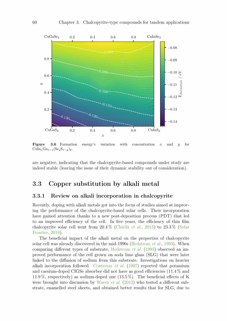
60 Chapter 3. Chalcopyrite-type compounds for tandem applications
CuGaS2 0.2 0.4 0.6 0.8 CuInS2
x
0.2
0.4
0.6
0.8
y
-0.130-0.120
-0.110
-0.100
-0.090
-0.080
CuGaSe2 0.2 0.4 0.6 0.8 CuInSe2
−0.14
−0.13
−0.12
−0.11
−0.10
−0.09
−0.08
Eformation
/eV
Figure 3.6 Formation energy’s variation with concentration x and y forCuInxGa1−x(SeyS1−y)2.
are negative, indicating that the chalcopyrite-based compounds under study areindeed stable (leaving the issue of their dynamic stability out of consideration).
3.3 Copper substitution by alkali metal
3.3.1 Review on alkali incorporation in chalcopyrite
Recently, doping with alkali metals got into the focus of studies aimed at improv-ing the performance of the chalcopyrite-based solar cells. Their incorporationhave gained attention thanks to a new post-deposition process (PDT) that ledto an improved efficiency of the cell. In five years, the efficiency of thin filmchalcopyrite solar cell went from 20.4 % (Chirilă et al., 2013) to 23.3 % (SolarFrontier, 2019).
The beneficial impact of the alkali metal on the properties of chalcopyritesolar cell was already discovered in the mid-1990s (Hedstrom et al., 1993). Whencomparing different types of substrate, Hedstrom et al. (1993) observed an im-proved performance of the cell grown on soda lime glass (SLG) that were laterlinked to the diffusion of sodium from this substrate. Investigations on heavieralkali incorporation followed. Contreras et al. (1997) reported that potassiumand caesium-doped CIGSe absorber did not have as good efficiencies (11.4 % and11.9 %, respectively) as sodium-doped one (13.5 %). The beneficial effects of Kwere brought into discussion by Wuerz et al. (2012) who tested a different sub-strate, enamelled steel sheets, and obtained better results that for SLG, due to
3.3. Copper substitution by alkali metal 61
the higher concentration of potassium. Since then, potassium, rubidium and cae-sium were tried, that pushed the efficiency record even further. A number ofreview articles summarise the influence of the alkali incorporation in chalcopy-rites (Salomé et al., 2015; Muzzillo, 2017; Sun et al., 2017).
Sodium incorporation into CIGS absorber modifies the latter’s properties in anumber of ways. The major modification is the increase of the hole net concentra-tion (Cho et al., 2012; Rudmann et al., 2004), whereupon follows the increase ofthe fill factor (FF) and the open circuit voltage (Voc) (Rau et al., 1998; Granathet al., 2000; Cho et al., 2012). The same effects, yet with superior FF and Voc
than with sodium doping, were observed with potassium (Pianezzi et al., 2014;Khatri et al., 2016; Laemmle et al., 2013; Wuerz et al., 2012). The exact origin ofthe increase of the p-doping with the increase of the net hole concentration for Na(Cho et al., 2012; Rudmann et al., 2004) and K (Laemmle et al., 2013; Pianezziet al., 2014; Khatri et al., 2016) doping is still under debate. Different hypothesisare discussed in the literature. First, Na annihilates donor states, especially InCu.When competing for a Cu site, Na or K are more likely to take the place thanIn or Ga, so that the alkali incorporation lowers the InCu or GaCu concentration(Contreras et al., 1997; Laemmle et al., 2013; Shin et al., 2016). Secondly, asproposed by Niles et al. (1997), Na takes the place of In or Ga in CIGS in orderto create NaIn/Ga. The third hypothesis is that sodium enhanced the formationof oxyde at the surface and passivates selenium vacancies (Ruckh et al., 1996;Kronik et al., 1998); moreover, the oxygen substitutes for selenium vacancies.Finally, Yuan et al. (2016) proposed a mechanism in which sodium in copper siteout-diffuses during the cooling down, thus increasing the concentration of coppervacancies (VCu) and the net hole concentrations. Furthermore, the reduction ofthe thickness of the CdS layer is permitted thanks to potassium incorporationwith a better diffusion of Cd into the absorber (Chirilă et al., 2013), that leadsto a decrease of the optical loss and thus to an increase of the short circuit cur-rent. Potassium doping has an influence of the composition and structure nearthe surface (Muzzillo, 2017). For example, a Cu and Ga depleted zone appears(Chirilă et al., 2013), or a layer of a new material containing K is formed at theinterface (Handick et al., 2017). The Ga gradient becomes larger while increasingthe Na (Ishizuka et al., 2009) or K concentration (Laemmle et al., 2015; Wuerzet al., 2012).
The investigation of the heaviest alkali, rubidium and caesium, began withthe work of Jackson et al. (2016). As in the case of the lighter alkali, this resultedin an increase of the open circuit voltage (Wuerz et al., 2018; Karki et al., 2019;Weiss et al., 2018; Schöppe et al., 2017), the fill factor (Kato et al., 2018; Wuerzet al., 2018) and of the majority carrier concentration (Wuerz et al., 2018; Karkiet al., 2019) of the cell. However, the gain in the open circuit voltage has beenobserved to be more (Wuerz et al., 2018) or less (Jackson et al., 2016) importantthan the one of the sodium post-deposition treatment. Ishizuka et al. (2018) foundthat the Voc and fill factor increase whereas the short circuit current decreases forindium-based chalcopyrite, whereas they have found the opposite trends for the
62 Chapter 3. Chalcopyrite-type compounds for tandem applications
gallium-based compound. As Na and K (Khatri et al., 2016), Rb also increasesthe carrier lifetime (Karki et al., 2019). Just like potassium, rubidium has animportant impact on the morphology and the composition of the surface. Thereduction of the Cu and Ga concentration near the surface (Maticiuc et al., 2018)and formation of a RbInSe2 compound at the CIGS/CdS interface was directlyobserved using TEM measurements (Taguchi et al., 2018; Maticiuc et al., 2018;Kodalle et al., 2018). More recently, a number of works addressed the effect ofdoping with caesium (Jackson et al., 2016; Kim et al., 2018).
As the incorporation of alkali in chalcopyrite begun with sodium and con-tinued with heavier alkali, lithium incorporation was less studied than the rest ofthe family. Lithium incorporation in ternary chalcopyrites was investigated exper-imentally and theoretically (Maeda et al., 2017; Kusumoto et al., 2019; Rong-Tieet al., 2017; Boehnke and Neumann, 1992). The chalcopyrite phase sustains upto 10 % of Li on Cu sites in case of CuInS2 (Maeda et al., 2017; Kusumoto et al.,2019), 20 % for CuGaS2 (Maeda et al., 2017; Kusumoto et al., 2019), 40 % forCu(In,Ga)(S,Se)2(Rong-Tie et al., 2017) and even 50 % for CuInSe2 (Boehnkeand Neumann, 1992). At higher concentration, the chalcopyrite phase coexistswith the orthorhombic one corresponding to the Li(In,Ga)(S,Se)2 compound.
Combining different alkali offers an additional option potentially useful forbetter performances (Chirilă et al., 2013; Kim et al., 2018). However, ion ex-change mechanism takes place inside the absorber. This is the case for K thattends to replace Na (Chirilă et al., 2013) or Rb that pushes away lighter alkali(Jackson et al., 2016; Vilalta-Clemente et al., 2018; Kodalle et al., 2018; Maticiucet al., 2018). That mechanism is not yet well understood.
The origin of the beneficial effect of alkali on the solar cell efficiency is stillunclear (Oikkonen et al., 2013; Mungan et al., 2013). It seems difficult to pin-point whether the effect primarily stems from the grain boundaries (Urbaniaket al., 2014) or from inside the bulk (Yuan et al., 2016; Wei et al., 1999), as alkalihave been found in both these locations (Laemmle et al., 2014; Forest et al., 2017;Cojocaru-Mirédin et al., 2011; Cojocaru-Mirédin et al., 2013; Schöppe et al., 2017;Wuerz et al., 2018; Kodalle et al., 2018). The presence of different alkali plays acrucial role in the diffusivity inside the absorber as it has been proved by Wuerzet al. (2018) by means of secondary ion mass spectrometry.
Compositions and defects were characterised by different techniques such asscanning electron microscopy (Eid et al., 2015; Kodalle et al., 2018) or secondaryion mass spectrometry (Eid et al., 2015). Werner et al. (2018) have shown thatthe electronic effects due to alkali doping in chalcopyrite absorbers are not char-acterisable today because of the strong influence of the buffer/window stack. Fordeeper understanding or predictions, first-principles studies have to be performed.
There are only few papers that discussed the incorporation of alkali metalon CIGS from a theoretical point of view. The majority of these papers are con-cerned with chalcopyrite ternary compounds and particularly CuInSe2 (Oikkonenet al., 2013; Ghorbani et al., 2015; Malitckaya et al., 2017). In order to explain the
3.3. Copper substitution by alkali metal 63
evolution of properties due to alkali doping, different parameters are calculatedsuch as the band gap, lattice constants, or the absorption coefficient. The prop-erties of the major interest for us will be the formation energies for different in-corporations possible like AlkCu, AlkIn/Ga, Alki etc. with Alk = (Li,Na,K,Rb,Cs).
First of all, alkali metals substitute either the cation or the anion. In all thecalculation done, the anion substitution has a very high formation energy [higherthan 1.2 eV -see Malitckaya et al. (2017)] that makes it very unlikely to occur,except maybe at considerable anion deficiency. An alkali element would thereforesubstitute either copper or indium/gallium. In the first case, the formal valencestate is not changed on substitution, whereas in the second case the univalentCu will substitute an atom with three valent electrons, thus resulting in two elec-trons missing and effectively a +2-charged defect. In all previous studies, theneutral copper substitution was found to be the most favourable event. This canbe attributed to the covalent bond linking the anion and the copper atom beingrelatively weak (Oikkonen et al., 2013). The dumbbell configuration was foundpossible only for Li and Na at the copper site (Malitckaya et al., 2017). Theindium-based chalcopyrite has lower substitution energy than the gallium-basedone. This is the case for the substitution of In compared to the one of Ga butalso when copper is substituted: NaCu has a higher formation energy in CuGaSe2
compared to CuInSe2 (Maeda et al., 2015). This substitution does not directlyexplain the observed increase of the net hole concentration on the chalcopyritecompound after alkali-fluoride PDT. AlkIn/Ga could explain this increase of con-centration but it is not the preponderant defect in the material. However, thesubstitution energy of indium in copper site by sodium is lower than the one ofcopper, so that sodium may first decrease the concentration of InCu defects andthus increase the net hole concentration (Wei et al., 1999). On the contrary, ifthe alkali take the place of copper vacancies, this decreases the net hole concen-tration.
An interstitial incorporation of the alcali metal atoms was also investigatedand found possible in the ternary compounds. Sodium (Oikkonen et al., 2013;Malitckaya et al., 2017) and heavier alkali (Malitckaya et al., 2017) occupiedpreferably the tetrahedral sites whereas lithium prefers octahedral sites. Ghor-bani et al. (2015) added that Na is more likely to go to the tetrahedral sitesurrounded by two cations and two anions, whereas K prefers the one completelysurrounded by cations. Yet, all these interstitial incorporations have higher for-mation energy than the copper substitution, and thus less likely to happen. Thediffusion mechanisms of these point defects inside the bulk were also discussedbut are beyond the scope of the present work.
All the theoretical investigations cited were performed on isolated point de-fects, and the effect of concentration was extrapolated. In the following, wesystematically and explicitly investigate the impact of alkali concentration in-side the bulk. That leads to a more detailed picture of the alkali incorporationthroughout a broad range of composition. We start with the most stable defecton the literature, the neutral substitution of copper by alkali metals.
64 Chapter 3. Chalcopyrite-type compounds for tandem applications
3.3.2 Influence of the substitutions on the crystals struc-tures
The methodology used to generate the different substitutions have been discussedin details in the previous section. The table 3.1 summarises the different initialsupercells used in this work. It gives their lattice parameters, the supercell ex-pansion matrices with respect to the primitive cell, the list of the irreducible Cusites and the number of sites equivalent by symmetry for each of them, as wellas the Monkhorst-Pack k-points meshes (Monkhorst and Pack, 1976) applied ineach case. Except for the primitive cell (space group I 42d), the space group ofeach supercell is P 4. In total, 12 different concentrations have been probed for atotal of 50 configurations of different symmetries. In the following, the obtainedresults are discussed in terms of pseudo-conventional tetragonal parameters evo-lution and tetrahedra’s deformation.
The Figure 3.8 shows the relative modifications of the lattice parameters (a/a0,b/b0, c/c0) induced by the copper substitution by alkali metals. The obtainedtrends are in good agreement with experimental data, when available, as illus-trated by the Figure 3.7: for Cu1−xLix(Ga/In)(S/Se)2, with 0 < x < 0.60, ourcalculated lattice deformation are compared to the results of Kusumoto et al.(2019), Rong-Tie et al. (2017) and Maeda et al. (2017) on CuGaS2, CuInS2 andCuInSe2 respectively. The absolute error between our theoretical and experimen-tal data is less than 1 % for these three compounds. Other alkali incorporation atthese ranges of concentration has not yet been done experimentally, to our bestknowledge.
In general, with the rate of substitution, the lattice parameters vary in a nottrivial way. For K, Na, Rb and Cs substituted chalcopyrite, the lattice parametersa and b increase when c decreases as the alkali metal concentration grows. Thisis also true for CuGa(S/Se)2 substituted with Li; however, it is not the case forthe two indium-based compounds, in which, as copper is replaced by lithium, thec parameters grows as well, albeit less pronouncedly than a and b (within 1 %).
0.0 0.1 0.2 0.3 0.4 0.5 0.6
Alkali concentration (x)
0.990
0.995
1.000
1.005
1.010
1.015
1.020
Lat
tice
def
orm
atio
n(a a0,b b 0
,c c 0
) a)
0.0 0.1 0.2 0.3 0.4 0.5 0.6
Alkali concentration (x)
b)
0.0 0.1 0.2 0.3 0.4 0.5 0.6
Alkali concentration (x)
c)
Figure 3.7 Comparison between the calculated and experimental(Kusumoto et al., 2019;Rong-Tie et al., 2017; Maeda et al., 2017) lattice deformations, a
a0(•), b
b0(•) and c
c0(•) of
a) Cu1−xLixGaS2, b) Cu1−xLixInS2 and c) Cu1−xLixInSe2. The experimental aa0
and cc0
arerepresented by H and by N, respectively.
3.3. Copper substitution by alkali metal 65
Table 3.1 Construction of the supercells used in the calculations. The indices P and C standfor primitive and conventional, respectively. The supercell expansion matrices refer to theprimitive lattice vectors. The fractional coordinates (x, y, z) of the irreducible sites of copperas well as their multiplicity (M , number of equivalent sites) in the supercells are given. TheMonkhorst-Pack k-points meshes (Monkhorst and Pack, 1976) (k) to realise the optimisationof the structures are also provided.
Number Space Lattice Supercell Irreducible M. k
of group parameter expansion Cu sitesatoms matrix (x, y, z)
8 I 42d a = b = c = aP
1 0 0
0 1 0
0 0 1
1 - (0, 0, 0) 2 18
α = β = αP
γ = γP
16 P 4 a = aC
0 1 1
1 0 1
1 1 0
1 - (0, 0, 0) 1 12
c = cC 2 - (12 ,
12 ,
12) 1
3 - (12 , 0,
14) 2
32 P 4 a =√
2 · aC
1 1 2
1 −1 0
1 1 0
1 - (0, 0, 0) 1 10
c = cC 2 - (12 ,
12 , 0) 1
3 - (12 , 0,
12) 2
4 - (34 ,
14 ,
34) 4
64 P 4 a = 2 · aC
2 0 2
0 −2 −2
1 1 0
1 - (0, 12 , 0) 2 8
c = cC 2 -(12 ,
12 , 0) 1
3 - (0, 0, 0) 1
4 - (34 ,
14 ,
12) 4
5 - (12 ,
34 ,
34) 4
6 - (0, 14 ,
34) 4
128 P 4 a = 2 · aC
0 2 2
2 0 2
2 2 0
1 - (0, 0, 0) 1 6
c = 2 · cC 2 - (0, 0, 12) 1
3 - (0, 12 , 0) 2
4 - (0, 12 ,
12) 2
5 - (12 ,
12 , 0) 1
6 - (12 ,
12 ,
12) 1
7 - (34 ,
14 ,
14) 4
8 - (34 ,
14 ,
34) 4
9 - (14 , 0,
78) 4
10 - (14 , 0,
38) 4
11 - (14 ,
12 ,
78) 4
12 - (14 ,
12 ,
38) 4
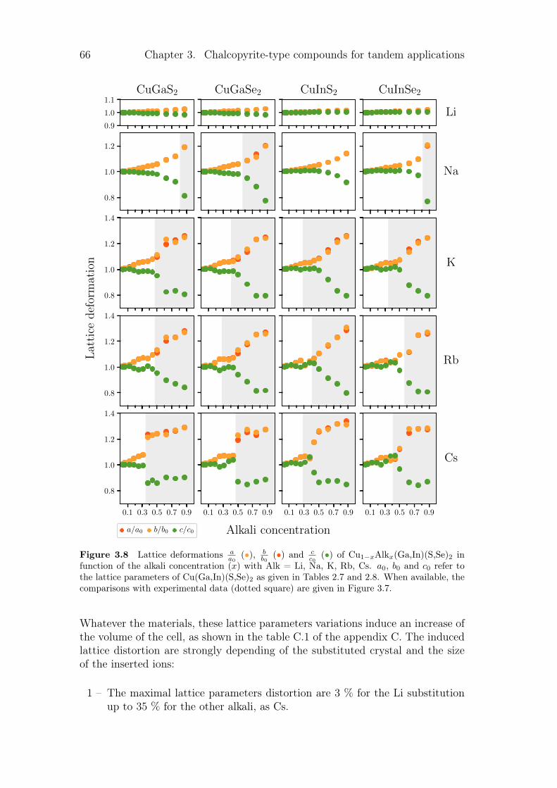
66 Chapter 3. Chalcopyrite-type compounds for tandem applications
0.9
1.0
1.1CuGaS2 CuGaSe2 CuInS2 CuInSe2
Li
0.8
1.0
1.2
Na
0.8
1.0
1.2
1.4
Lat
tice
def
orm
atio
n K
0.8
1.0
1.2
1.4
Rb
0.1 0.3 0.5 0.7 0.9
0.8
1.0
1.2
1.4
a/a0 b/b0 c/c0
0.1 0.3 0.5 0.7 0.9
Alkali concentration
0.1 0.3 0.5 0.7 0.9 0.1 0.3 0.5 0.7 0.9
Cs
Figure 3.8 Lattice deformations aa0
(•), bb0
(•) and cc0
(•) of Cu1−xAlkx(Ga,In)(S,Se)2 infunction of the alkali concentration (x) with Alk = Li, Na, K, Rb, Cs. a0, b0 and c0 refer tothe lattice parameters of Cu(Ga,In)(S,Se)2 as given in Tables 2.7 and 2.8. When available, thecomparisons with experimental data (dotted square) are given in Figure 3.7.
Whatever the materials, these lattice parameters variations induce an increase ofthe volume of the cell, as shown in the table C.1 of the appendix C. The inducedlattice distortion are strongly depending of the substituted crystal and the sizeof the inserted ions:
1 – The maximal lattice parameters distortion are 3 % for the Li substitutionup to 35 % for the other alkali, as Cs.
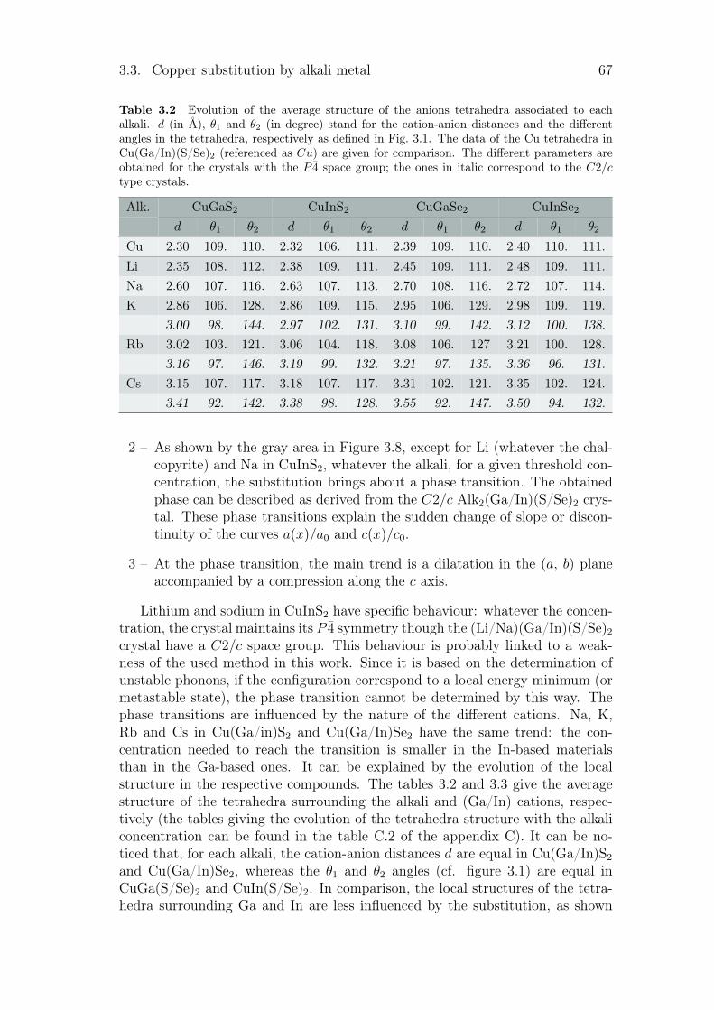
3.3. Copper substitution by alkali metal 67
Table 3.2 Evolution of the average structure of the anions tetrahedra associated to eachalkali. d (in Å), θ1 and θ2 (in degree) stand for the cation-anion distances and the differentangles in the tetrahedra, respectively as defined in Fig. 3.1. The data of the Cu tetrahedra inCu(Ga/In)(S/Se)2 (referenced as Cu) are given for comparison. The different parameters areobtained for the crystals with the P 4 space group; the ones in italic correspond to the C2/ctype crystals.
Alk. CuGaS2 CuInS2 CuGaSe2 CuInSe2
d θ1 θ2 d θ1 θ2 d θ1 θ2 d θ1 θ2
Cu 2.30 109. 110. 2.32 106. 111. 2.39 109. 110. 2.40 110. 111.Li 2.35 108. 112. 2.38 109. 111. 2.45 109. 111. 2.48 109. 111.Na 2.60 107. 116. 2.63 107. 113. 2.70 108. 116. 2.72 107. 114.K 2.86 106. 128. 2.86 109. 115. 2.95 106. 129. 2.98 109. 119.
3.00 98. 144. 2.97 102. 131. 3.10 99. 142. 3.12 100. 138.Rb 3.02 103. 121. 3.06 104. 118. 3.08 106. 127 3.21 100. 128.
3.16 97. 146. 3.19 99. 132. 3.21 97. 135. 3.36 96. 131.Cs 3.15 107. 117. 3.18 107. 117. 3.31 102. 121. 3.35 102. 124.
3.41 92. 142. 3.38 98. 128. 3.55 92. 147. 3.50 94. 132.
2 – As shown by the gray area in Figure 3.8, except for Li (whatever the chal-copyrite) and Na in CuInS2, whatever the alkali, for a given threshold con-centration, the substitution brings about a phase transition. The obtainedphase can be described as derived from the C2/c Alk2(Ga/In)(S/Se)2 crys-tal. These phase transitions explain the sudden change of slope or discon-tinuity of the curves a(x)/a0 and c(x)/c0.
3 – At the phase transition, the main trend is a dilatation in the (a, b) planeaccompanied by a compression along the c axis.
Lithium and sodium in CuInS2 have specific behaviour: whatever the concen-tration, the crystal maintains its P 4 symmetry though the (Li/Na)(Ga/In)(S/Se)2
crystal have a C2/c space group. This behaviour is probably linked to a weak-ness of the used method in this work. Since it is based on the determination ofunstable phonons, if the configuration correspond to a local energy minimum (ormetastable state), the phase transition cannot be determined by this way. Thephase transitions are influenced by the nature of the different cations. Na, K,Rb and Cs in Cu(Ga/in)S2 and Cu(Ga/In)Se2 have the same trend: the con-centration needed to reach the transition is smaller in the In-based materialsthan in the Ga-based ones. It can be explained by the evolution of the localstructure in the respective compounds. The tables 3.2 and 3.3 give the averagestructure of the tetrahedra surrounding the alkali and (Ga/In) cations, respec-tively (the tables giving the evolution of the tetrahedra structure with the alkaliconcentration can be found in the table C.2 of the appendix C). It can be no-ticed that, for each alkali, the cation-anion distances d are equal in Cu(Ga/In)S2
and Cu(Ga/In)Se2, whereas the θ1 and θ2 angles (cf. figure 3.1) are equal inCuGa(S/Se)2 and CuIn(S/Se)2. In comparison, the local structures of the tetra-hedra surrounding Ga and In are less influenced by the substitution, as shown
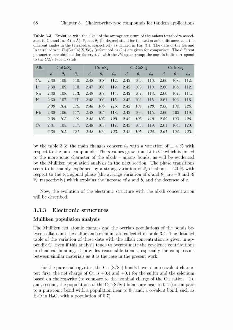
68 Chapter 3. Chalcopyrite-type compounds for tandem applications
Table 3.3 Evolution with the alkali of the average structure of the anions tetrahedra associ-ated to Ga and In. d (in Å), θ1 and θ2 (in degree) stand for the cation-anion distances and thedifferent angles in the tetrahedra, respectively as defined in Fig. 3.1. The data of the Ga andIn tetrahedra in Cu(Ga/In)(S/Se)2 (referenced as Cu) are given for comparison. The differentparameters are obtained for the crystals with the P 4 space group; the ones in italic correspondto the C2/c type crystals.
Alk. CuGaS2 CuInS2 CuGaSe2 CuInSe2
d θ1 θ2 d θ1 θ2 d θ1 θ2 d θ1 θ2
Cu 2.30 109. 110. 2.48 108. 112. 2.42 109. 110. 2.60 108. 112.Li 2.30 109. 110. 2.47 108. 112. 2.42 109. 110. 2.60 108. 112.Na 2.30 108. 113. 2.48 107. 114. 2.42 107. 113. 2.60 107. 114.K 2.30 107. 117.. 2.48 106. 115. 2.42 106. 115. 2.61 106. 116.
2.30 104. 119. 2.48 106. 115. 2.42 104. 120. 2.60 104. 120.Rb 2.30 106. 117. 2.48 105. 118. 2.42 106. 115. 2.60 105 119.
2.30 105. 119. 2.48 105. 120. 2.42 105. 119. 2.59 103. 126.Cs 2.31 105. 117. 2.48 105. 117. 2.43 105. 119. 2.61 104. 120.
2.30 105. 121. 2.48 104. 123. 2.42 105. 124. 2.61 104. 123.
by the table 3.3: the main changes concern θ2 with a variation of ± 4 % withrespect to the pure compounds. The d values grow from Li to Cs which is linkedto the more ionic character of the alkali – anions bonds, as will be evidencedby the Mulliken population analysis in the next section. The phase transitionsseem to be mainly explained by a strong variation of θ2 of about + 20 % withrespect to the tetragonal phase (the average variation of d and θ1 are +8 and -9%, respectively) which explains the increase of a and b, and the decrease of c.
Now, the evolution of the electronic structure with the alkali concentrationwill be described.
3.3.3 Electronic structures
Mulliken population analysis
The Mulliken net atomic charges and the overlap populations of the bonds be-tween alkali and the sulfur and selenium are collected in table 3.4. The detailedtable of the variation of these date with the alkali concentration is given in ap-pendix C. Even if this analysis tends to overestimate the covalence contributionsin chemical bonding, it provides reasonable trends, especially for comparisonsbetween similar materials as it is the case in the present work.
For the pure chalcopyrites, the Cu-(S/Se) bonds have a iono-covalent charac-ter: first, the net charge of Cu is +0.4 and +0.1 for the sulfur and the seleniumbased on chalcopyrite (to compare to the nominal charge of the Cu cation +1),and, second, the populations of the Cu-(S/Se) bonds are near to 0.4 (to compareto a pure ionic bond with a population near to 0., and, a covalent bond, such asH-O in H2O, with a population of 0.7).
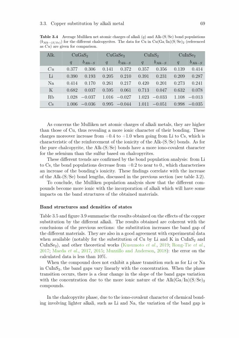
3.3. Copper substitution by alkali metal 69
Table 3.4 Average Mulliken net atomic charges of alkali (q) and Alk-(S/Se) bond populations(bAlk−(S/Se)) for the different chalcopyrites. The data for Cu in Cu(Ga/In)(S/Se)2 (referencedas Cu) are given for comparison.
Alk. CuGaS2 CuGaSe2 CuInS2 CuInSe2
q bAlk−S q bAlk−S q bAlk−S q bAlk−S
Cu 0.377 0.306 0.141 0.372 0.357 0.356 0.139 0.414
Li 0.390 0.193 0.205 0.210 0.391 0.231 0.209 0.287
Na 0.414 0.170 0.261 0.217 0.420 0.201 0.273 0.241
K 0.682 0.037 0.595 0.061 0.713 0.047 0.632 0.078
Rb 1.028 −0.037 1.016 −0.027 1.023 −0.033 1.108 −0.013
Cs 1.006 −0.036 0.995 −0.044 1.011 −0.051 0.998 −0.035
As concerns the Mulliken net atomic charges of alkali metals, they are higherthan those of Cu, thus revealing a more ionic character of their bonding. Thesecharges moreover increase from +0.4 to +1.0 when going from Li to Cs, which ischaracteristic of the reinforcement of the ionicity of the Alk-(S/Se) bonds. As forthe pure chalcopyrite, the Alk-(S/Se) bonds have a more iono-covalent characterfor the selenium than the sulfur based on chalcopyrites.
These different trends are confirmed by the bond population analysis: from Lito Cs, the bond populations decrease from +0.2 to near to 0., which characterisesan increase of the bonding’s ionicity. These findings correlate with the increaseof the Alk-(S/Se) bond lengths, discussed in the previous section (see table 3.2).
To conclude, the Mulliken population analysis show that the different com-pounds become more ionic with the incorporation of alkali which will have someimpacts on the band structures of the obtained materials.
Band structures and densities of states
Table 3.5 and figure 3.9 summarise the results obtained on the effects of the coppersubstitution by the different alkali. The results obtained are coherent with theconclusions of the previous sections: the substitution increases the band gap ofthe different materials. They are also in a good agreement with experimental datawhen available (notably for the substitution of Cu by Li and K in CuInS2 andCuInSe2), and other theoretical works (Kusumoto et al., 2019; Rong-Tie et al.,2017; Maeda et al., 2017, 2015; Muzzillo and Anderson, 2018): the error on thecalculated data is less than 10%.
When the compound does not exhibit a phase transition such as for Li or Nain CuInS2, the band gaps vary linearly with the concentration. When the phasetransition occurs, there is a clear change in the slope of the band gaps variationwith the concentration due to the more ionic nature of the Alk(Ga/In)(S/Se)2
compounds.
In the chalcopyrite phase, due to the iono-covalent character of chemical bond-ing involving lighter alkali, such as Li and Na, the variation of the band gap is
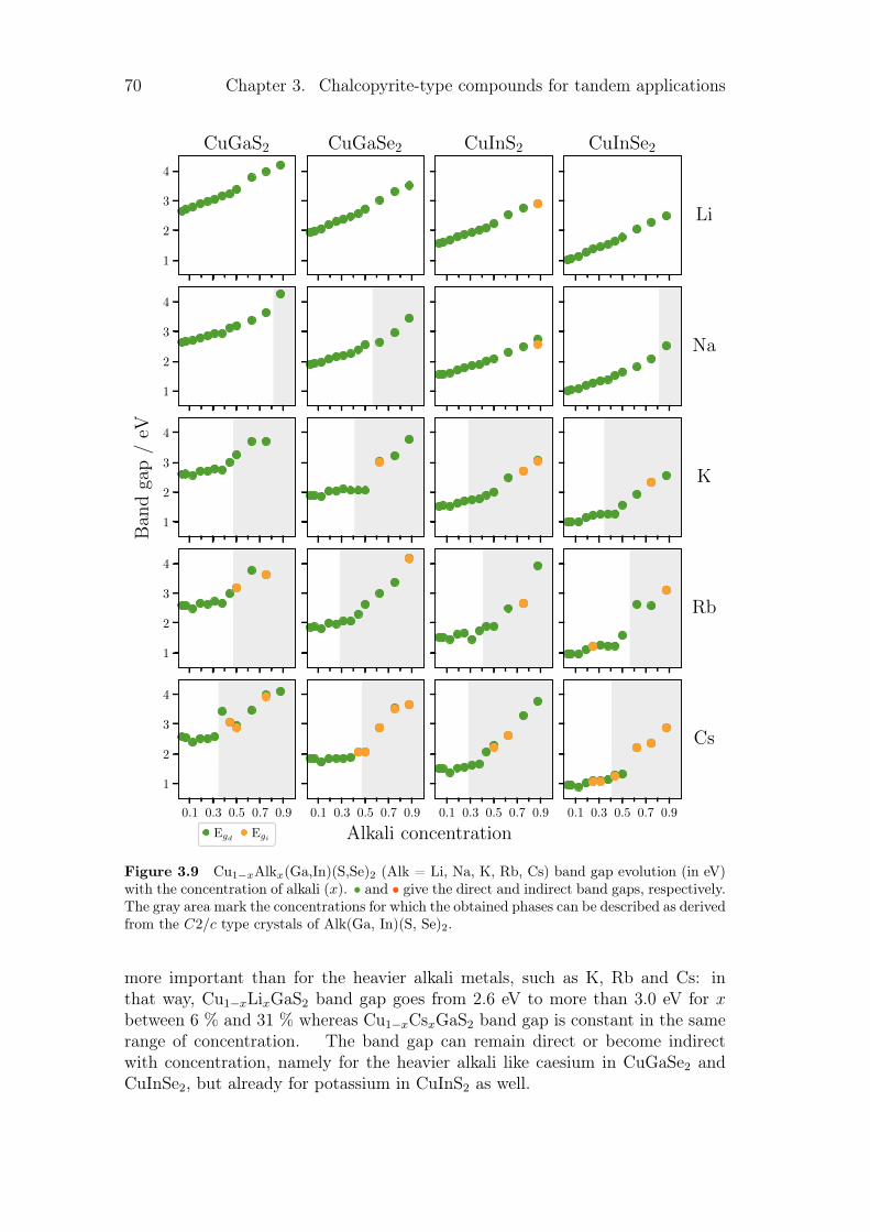
70 Chapter 3. Chalcopyrite-type compounds for tandem applications
1
2
3
4
CuGaS2 CuGaSe2 CuInS2 CuInSe2
Li
1
2
3
4
Na
1
2
3
4
Ban
dga
p/
eV
K
1
2
3
4
Rb
0.1 0.3 0.5 0.7 0.9
1
2
3
4
Egd Egi
0.1 0.3 0.5 0.7 0.9
Alkali concentration0.1 0.3 0.5 0.7 0.9 0.1 0.3 0.5 0.7 0.9
Cs
Figure 3.9 Cu1−xAlkx(Ga,In)(S,Se)2 (Alk = Li, Na, K, Rb, Cs) band gap evolution (in eV)with the concentration of alkali (x). • and • give the direct and indirect band gaps, respectively.The gray area mark the concentrations for which the obtained phases can be described as derivedfrom the C2/c type crystals of Alk(Ga, In)(S, Se)2.
more important than for the heavier alkali metals, such as K, Rb and Cs: inthat way, Cu1−xLixGaS2 band gap goes from 2.6 eV to more than 3.0 eV for xbetween 6 % and 31 % whereas Cu1−xCsxGaS2 band gap is constant in the samerange of concentration. The band gap can remain direct or become indirectwith concentration, namely for the heavier alkali like caesium in CuGaSe2 andCuInSe2, but already for potassium in CuInS2 as well.
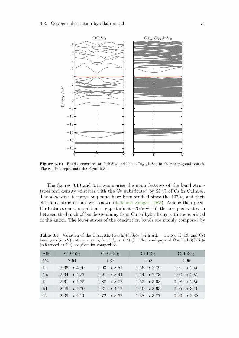
3.3. Copper substitution by alkali metal 71
T Γ N
−18
−16
−14
−12
−10
−8
−6
−4
−2
0
2
4
6
8
En
ergy
/eV
T Γ N
Cu0.75Cs0.25InSe2CuInSe2
Figure 3.10 Bands structures of CuInSe2 and Cu0.75Cs0.25InSe2 in their tetragonal phases.The red line represents the Fermi level.
The figures 3.10 and 3.11 summarise the main features of the band struc-tures and density of states with the Cu substituted by 25 % of Cs in CuInSe2.The alkali-free ternary compound have been studied since the 1970s, and theirelectronic structure are well known (Jaffe and Zunger, 1983). Among their pecu-liar features one can point out a gap at about −3 eV within the occupied states, inbetween the bunch of bands stemming from Cu 3d hybridising with the p orbitalof the anion. The lower states of the conduction bands are mainly composed by
Table 3.5 Variation of the Cu1−xAlkx(Ga/In)(S/Se)2 (with Alk = Li, Na, K, Rb and Cs)band gap (in eV) with x varying from 1
16 to (→) 78 . The band gaps of Cu(Ga/In)(S/Se)2
(referenced as Cu) are given for comparison.
Alk. CuGaS2 CuGaSe2 CuInS2 CuInSe2
Cu 2.61 1.87 1.52 0.96Li 2.66 → 4.20 1.93 → 3.51 1.56 → 2.89 1.01 → 2.46Na 2.64 → 4.27 1.91 → 3.44 1.54 → 2.73 1.00 → 2.52K 2.61 → 4.75 1.88 → 3.77 1.53 → 3.08 0.98 → 2.56Rb 2.49 → 4.70 1.81 → 4.17 1.46 → 3.93 0.95 → 3.10Cs 2.39 → 4.11 1.72 → 3.67 1.38 → 3.77 0.90 → 2.88
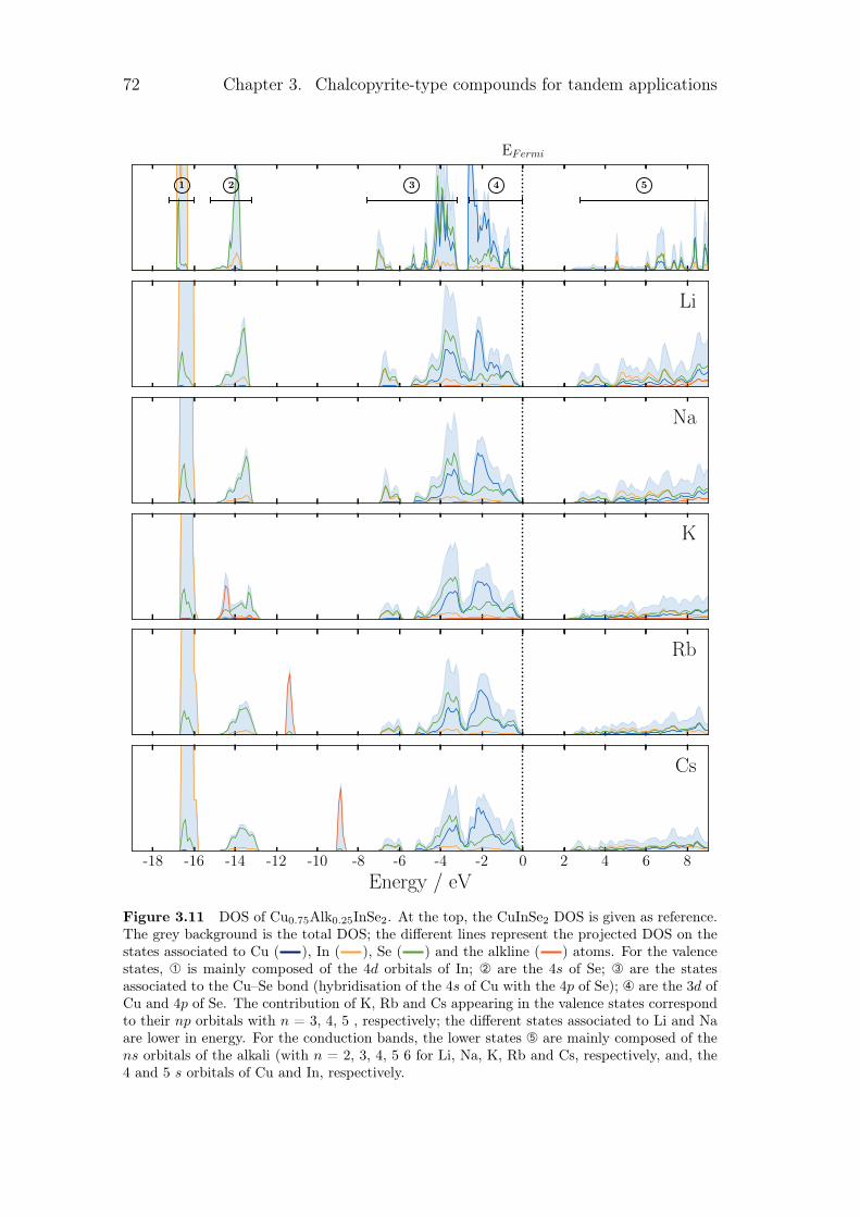
72 Chapter 3. Chalcopyrite-type compounds for tandem applications
1 2 3 4 5
EFermi
Li
Na
K
Rb
-18 -16 -14 -12 -10 -8 -6 -4 -2 0 2 4 6 8
Energy / eV
Cs
Figure 3.11 DOS of Cu0.75Alk0.25InSe2. At the top, the CuInSe2 DOS is given as reference.The grey background is the total DOS; the different lines represent the projected DOS on thestates associated to Cu ( ), In ( ), Se ( ) and the alkline ( ) atoms. For the valencestates, À is mainly composed of the 4d orbitals of In; Á are the 4s of Se; Â are the statesassociated to the Cu–Se bond (hybridisation of the 4s of Cu with the 4p of Se); Ã are the 3d ofCu and 4p of Se. The contribution of K, Rb and Cs appearing in the valence states correspondto their np orbitals with n = 3, 4, 5 , respectively; the different states associated to Li and Naare lower in energy. For the conduction bands, the lower states Ä are mainly composed of thens orbitals of the alkali (with n = 2, 3, 4, 5 6 for Li, Na, K, Rb and Cs, respectively, and, the4 and 5 s orbitals of Cu and In, respectively.
3.3. Copper substitution by alkali metal 73
the empty s orbitals of Cu, Ga and In.
The use of supercells with a partial loss of symmetry lifts the degeneracyof different bands. The main effects on the substitution is the appearance of anisolated state associated to the p orbitals of K, Rb, Cs at −9, −11 and −14 eV,respectively; the s orbital of Li and p orbitals are deeper at -30 eV. The changeof bonding, depending on the concentration, can lead to the disappearance ofthe gap between the p orbitals of S/Se and the d orbitals of Cu. The increaseof the band gap is mainly due to the shift towards higher energies of the lowestconduction bands, linked to the increase of the empty s alkali’s orbitals rate tothese bands.
Recollecting that the target of this work is the design of materials for tandemapplication with an optimal band gap in the range 1.5 – 1.7 eV, we note thatonly the indium-based chalcopyrites reach this criteria. Let’s consider now theirthermodynamical properties.
3.3.4 Thermodynamical properties of the substituted chal-copyrites
Energies of copper substitution by alkali metals
In order to evaluate the feasibility of the copper substitution by alkali metals, thecorresponding energy needs to be evaluated as a function of x. In our case, thefollowing chemical reactions have been considered to determine the substitutionenergy of copper:
xAlk + CuAB2 → xCu + Cu1−xAlkxAB2, (3.5)
with Alk = Li, Na, K, Rb and Cs; A = Ga and In, and, B = S and Se. Thesubstitution energy is then
Ef = ECu1−xAlkxAB2
tot + x× ECu − ECuAB2tot − x× EAlk, (3.6)
where ECu1−xAlkxAB2
tot is the total energy of the defective supercell normalised bythe number of CuAB2 moities in the cell, ECuAB2
tot is the total energy of one CuAB2,and ECu and EAlk the total energies of the isolated atoms in their fundamentalstates. The zero point energy was taken into account here, differently from theenergy calculations reported in section 3.2. The calculated substitutions energiesare plotted in figure 3.12.
For all substituting alkali metals, the formation energy exhibits the sametrend: it initially increases until it reaches a maximum around 10 %, and thendecreases. At low concentration, it is more difficult to substitute copper by analkali metal, whereas at high concentration, with the joint effect of the cell ex-pansion and phase transitions, the incorporation is easier.
Two groups of alkali metals can be distinguished: whereas the lighter ones (Li,Na and K) are characterised by formation energies lower than 2 eV, the formationenergy of the heavier ones (Rb and Cs) is above 3 eV. The substitution energies for
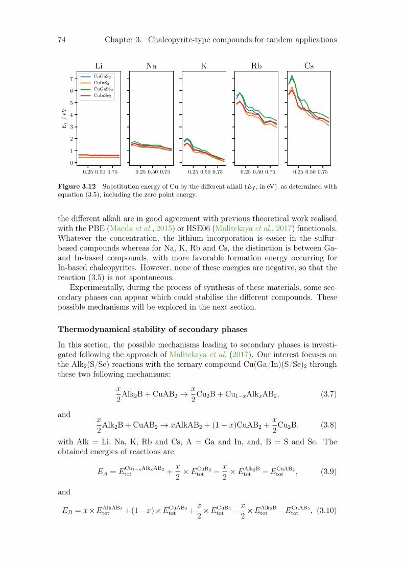
74 Chapter 3. Chalcopyrite-type compounds for tandem applications
0.25 0.50 0.75
0
1
2
3
4
5
6
7
Ef
/eV
LiCuGaS2
CuInS2
CuGaSe2
CuInSe2
0.25 0.50 0.75
Na
0.25 0.50 0.75
K
0.25 0.50 0.75
Rb
0.25 0.50 0.75
Cs
Figure 3.12 Substitution energy of Cu by the different alkali (Ef , in eV), as determined withequation (3.5), including the zero point energy.
the different alkali are in good agreement with previous theoretical work realisedwith the PBE (Maeda et al., 2015) or HSE06 (Malitckaya et al., 2017) functionals.Whatever the concentration, the lithium incorporation is easier in the sulfur-based compounds whereas for Na, K, Rb and Cs, the distinction is between Ga-and In-based compounds, with more favorable formation energy occurring forIn-based chalcopyrites. However, none of these energies are negative, so that thereaction (3.5) is not spontaneous.
Experimentally, during the process of synthesis of these materials, some sec-ondary phases can appear which could stabilise the different compounds. Thesepossible mechanisms will be explored in the next section.
Thermodynamical stability of secondary phases
In this section, the possible mechanisms leading to secondary phases is investi-gated following the approach of Malitckaya et al. (2017). Our interest focuses onthe Alk2(S/Se) reactions with the ternary compound Cu(Ga/In)(S/Se)2 throughthese two following mechanisms:
x
2Alk2B + CuAB2 →
x
2Cu2B + Cu1−xAlkxAB2, (3.7)
andx
2Alk2B + CuAB2 → xAlkAB2 + (1− x)CuAB2 +
x
2Cu2B, (3.8)
with Alk = Li, Na, K, Rb and Cs; A = Ga and In, and, B = S and Se. Theobtained energies of reactions are
EA = ECu1−xAlkxAB2
tot +x
2× ECuB2
tot − x
2× EAlk2B
tot − ECuAB2tot , (3.9)
and
EB = x×EAlkAB2tot +(1−x)×ECuAB2
tot +x
2×ECuB2
tot − x2×EAlk2B
tot −ECuAB2tot , (3.10)
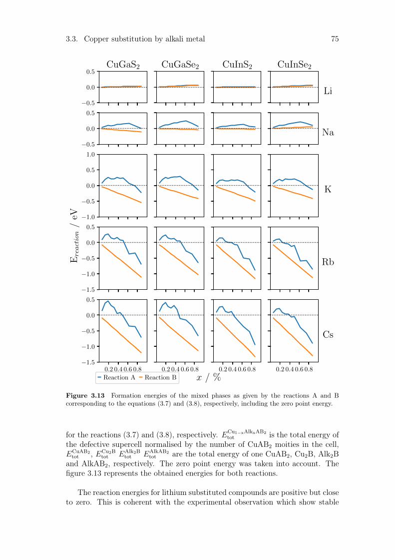
3.3. Copper substitution by alkali metal 75
−0.5
0.0
0.5
−0.5
0.0
0.5
−1.0
−0.5
0.0
0.5
1.0
Ereaction
/eV
−1.5
−1.0
−0.5
0.0
0.5
0.2 0.4 0.6 0.8−1.5
−1.0
−0.5
0.0
0.5
Reaction A Reaction B
0.2 0.4 0.6 0.8
x / %0.2 0.4 0.6 0.8 0.2 0.4 0.6 0.8
CuGaS2 CuGaSe2 CuInS2 CuInSe2
Li
Na
K
Rb
Cs
Figure 3.13 Formation energies of the mixed phases as given by the reactions A and Bcorresponding to the equations (3.7) and (3.8), respectively, including the zero point energy.
for the reactions (3.7) and (3.8), respectively. ECu1−xAlkxAB2
tot is the total energy ofthe defective supercell normalised by the number of CuAB2 moities in the cell,ECuAB2
tot , ECu2Btot EAlk2B
tot EAlkAB2tot are the total energy of one CuAB2, Cu2B, Alk2B
and AlkAB2, respectively. The zero point energy was taken into account. Thefigure 3.13 represents the obtained energies for both reactions.
The reaction energies for lithium substituted compounds are positive but closeto zero. This is coherent with the experimental observation which show stable
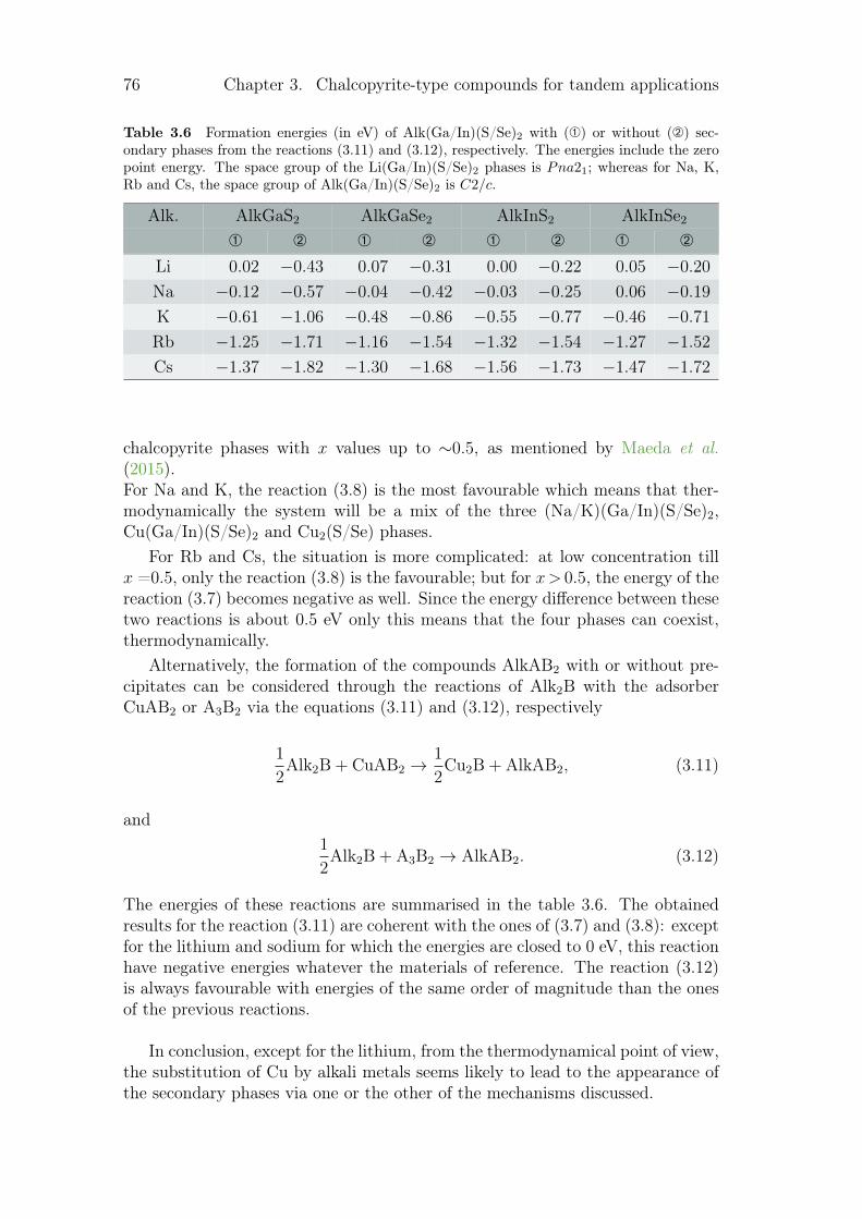
76 Chapter 3. Chalcopyrite-type compounds for tandem applications
Table 3.6 Formation energies (in eV) of Alk(Ga/In)(S/Se)2 with (À) or without (Á) sec-ondary phases from the reactions (3.11) and (3.12), respectively. The energies include the zeropoint energy. The space group of the Li(Ga/In)(S/Se)2 phases is Pna21; whereas for Na, K,Rb and Cs, the space group of Alk(Ga/In)(S/Se)2 is C2/c.
Alk. AlkGaS2 AlkGaSe2 AlkInS2 AlkInSe2
À Á À Á À Á À Á
Li 0.02 −0.43 0.07 −0.31 0.00 −0.22 0.05 −0.20
Na −0.12 −0.57 −0.04 −0.42 −0.03 −0.25 0.06 −0.19
K −0.61 −1.06 −0.48 −0.86 −0.55 −0.77 −0.46 −0.71
Rb −1.25 −1.71 −1.16 −1.54 −1.32 −1.54 −1.27 −1.52
Cs −1.37 −1.82 −1.30 −1.68 −1.56 −1.73 −1.47 −1.72
chalcopyrite phases with x values up to ∼0.5, as mentioned by Maeda et al.(2015).For Na and K, the reaction (3.8) is the most favourable which means that ther-modynamically the system will be a mix of the three (Na/K)(Ga/In)(S/Se)2,Cu(Ga/In)(S/Se)2 and Cu2(S/Se) phases.
For Rb and Cs, the situation is more complicated: at low concentration tillx =0.5, only the reaction (3.8) is the favourable; but for x> 0.5, the energy of thereaction (3.7) becomes negative as well. Since the energy difference between thesetwo reactions is about 0.5 eV only this means that the four phases can coexist,thermodynamically.
Alternatively, the formation of the compounds AlkAB2 with or without pre-cipitates can be considered through the reactions of Alk2B with the adsorberCuAB2 or A3B2 via the equations (3.11) and (3.12), respectively
1
2Alk2B + CuAB2 →
1
2Cu2B + AlkAB2, (3.11)
and1
2Alk2B + A3B2 → AlkAB2. (3.12)
The energies of these reactions are summarised in the table 3.6. The obtainedresults for the reaction (3.11) are coherent with the ones of (3.7) and (3.8): exceptfor the lithium and sodium for which the energies are closed to 0 eV, this reactionhave negative energies whatever the materials of reference. The reaction (3.12)is always favourable with energies of the same order of magnitude than the onesof the previous reactions.
In conclusion, except for the lithium, from the thermodynamical point of view,the substitution of Cu by alkali metals seems likely to lead to the appearance ofthe secondary phases via one or the other of the mechanisms discussed.
3.4. Summary and conclusion 77
3.4 Summary and conclusionOne of the key advantages of CIGS for photovoltaics is a possibility to con-trol their composition that leads to a tunability of different properties such asthe lattice parameter or the band gap. This feature makes chalcopyrite systempromising candidates for tandem application. At the beginning of this chapter,the influence of the penternary chalcopyrite CuInxGa1−x(SeyS1−y)2’s compositionon different properties was investigated. A complete mapping of the lattice pa-rameters, band gap and formation energy with the two concentrations x and ywas made. The target band gap values for photovoltaic applications are accessi-ble for higher concentration of indium than gallium. However, in this very rangeof concentrations, the lattice mismatch with silicon is quite appreciable, whereasa good matching with the silicon lattice parameter correspond to chalcopyritewith higher concentration of gallium and sulphur. Throughout these relevantcompositions, the system stays in the chalcopyrite symmetry, and its energy offormation is negative, thus the system remains thermodynamically stable.
In a similar method, alkali incorporation by means of cation substitution wassimulated. The first observation is that alkali metals increase the volume of thecell with an expansion of the lattice parameter a and a contraction of c. How-ever, the system goes from the P 4 symmetry at lowest concentration to C2/cfor the highest one, except in the case of doping with lithium and most of thecases concerning sodium; however, this might be due to an intrinsic issue of themethod. This deformation is purely due to the local deformation of the tetrahe-dra around the substituted atoms. The calculation of electronic properties werethen performed. The Mulliken population analysis shows that the different com-pounds become more ionic with the incorporation of alkali. As for the band gap,it increases with the concentration of alkali metal. That is not a good news forgallium-based ternary chalcopyrites that have band gap already larger than thetarget value, however might be useful for indium-based chalcopyrites to reach thetarget value. Different energy relations were then calculated corresponding tovarious chemical reactions. The main conclusion is that alkali metals incorpora-tion is not easy in chalcopyrite. Even if Li, Na and K have substitution energylower than 2 eV and hence much lower than Rb and Cs whose substitution energyis around 4 – 5 eV, all these energies are positive, and the substitution reaction isnot spontaneous. Moreover, except for the lithium, thermodynamically, the sub-stitution of the Cu by a alkali metals will lead to the appearance of the secondaryphases whatever the considered mechanisms.

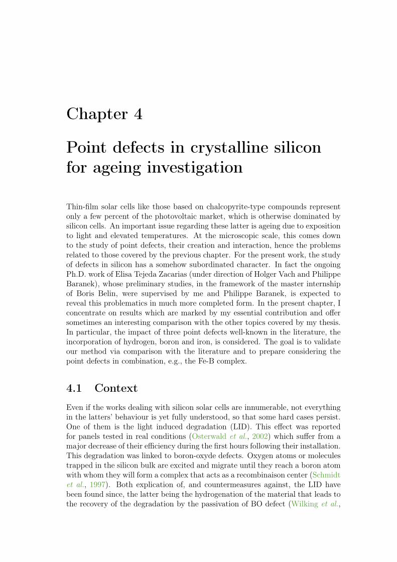
Chapter 4
Point defects in crystalline siliconfor ageing investigation
Thin-film solar cells like those based on chalcopyrite-type compounds representonly a few percent of the photovoltaic market, which is otherwise dominated bysilicon cells. An important issue regarding these latter is ageing due to expositionto light and elevated temperatures. At the microscopic scale, this comes downto the study of point defects, their creation and interaction, hence the problemsrelated to those covered by the previous chapter. For the present work, the studyof defects in silicon has a somehow subordinated character. In fact the ongoingPh.D. work of Elisa Tejeda Zacarias (under direction of Holger Vach and PhilippeBaranek), whose preliminary studies, in the framework of the master internshipof Boris Belin, were supervised by me and Philippe Baranek, is expected toreveal this problematics in much more completed form. In the present chapter, Iconcentrate on results which are marked by my essential contribution and offersometimes an interesting comparison with the other topics covered by my thesis.In particular, the impact of three point defects well-known in the literature, theincorporation of hydrogen, boron and iron, is considered. The goal is to validateour method via comparison with the literature and to prepare considering thepoint defects in combination, e.g., the Fe-B complex.
4.1 Context
Even if the works dealing with silicon solar cells are innumerable, not everythingin the latters’ behaviour is yet fully understood, so that some hard cases persist.One of them is the light induced degradation (LID). This effect was reportedfor panels tested in real conditions (Osterwald et al., 2002) which suffer from amajor decrease of their efficiency during the first hours following their installation.This degradation was linked to boron-oxyde defects. Oxygen atoms or moleculestrapped in the silicon bulk are excited and migrate until they reach a boron atomwith whom they will form a complex that acts as a recombinaison center (Schmidtet al., 1997). Both explication of, and countermeasures against, the LID havebeen found since, the latter being the hydrogenation of the material that leads tothe recovery of the degradation by the passivation of BO defect (Wilking et al.,
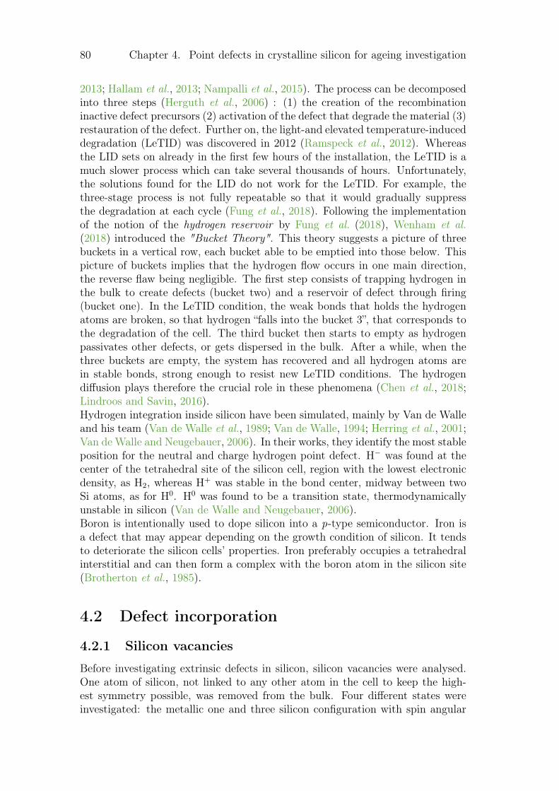
80 Chapter 4. Point defects in crystalline silicon for ageing investigation
2013; Hallam et al., 2013; Nampalli et al., 2015). The process can be decomposedinto three steps (Herguth et al., 2006) : (1) the creation of the recombinationinactive defect precursors (2) activation of the defect that degrade the material (3)restauration of the defect. Further on, the light-and elevated temperature-induceddegradation (LeTID) was discovered in 2012 (Ramspeck et al., 2012). Whereasthe LID sets on already in the first few hours of the installation, the LeTID is amuch slower process which can take several thousands of hours. Unfortunately,the solutions found for the LID do not work for the LeTID. For example, thethree-stage process is not fully repeatable so that it would gradually suppressthe degradation at each cycle (Fung et al., 2018). Following the implementationof the notion of the hydrogen reservoir by Fung et al. (2018), Wenham et al.(2018) introduced the "Bucket Theory". This theory suggests a picture of threebuckets in a vertical row, each bucket able to be emptied into those below. Thispicture of buckets implies that the hydrogen flow occurs in one main direction,the reverse flaw being negligible. The first step consists of trapping hydrogen inthe bulk to create defects (bucket two) and a reservoir of defect through firing(bucket one). In the LeTID condition, the weak bonds that holds the hydrogenatoms are broken, so that hydrogen “falls into the bucket 3”, that corresponds tothe degradation of the cell. The third bucket then starts to empty as hydrogenpassivates other defects, or gets dispersed in the bulk. After a while, when thethree buckets are empty, the system has recovered and all hydrogen atoms arein stable bonds, strong enough to resist new LeTID conditions. The hydrogendiffusion plays therefore the crucial role in these phenomena (Chen et al., 2018;Lindroos and Savin, 2016).Hydrogen integration inside silicon have been simulated, mainly by Van de Walleand his team (Van de Walle et al., 1989; Van de Walle, 1994; Herring et al., 2001;Van de Walle and Neugebauer, 2006). In their works, they identify the most stableposition for the neutral and charge hydrogen point defect. H− was found at thecenter of the tetrahedral site of the silicon cell, region with the lowest electronicdensity, as H2, whereas H+ was stable in the bond center, midway between twoSi atoms, as for H0. H0 was found to be a transition state, thermodynamicallyunstable in silicon (Van de Walle and Neugebauer, 2006).Boron is intentionally used to dope silicon into a p-type semiconductor. Iron isa defect that may appear depending on the growth condition of silicon. It tendsto deteriorate the silicon cells’ properties. Iron preferably occupies a tetrahedralinterstitial and can then form a complex with the boron atom in the silicon site(Brotherton et al., 1985).
4.2 Defect incorporation
4.2.1 Silicon vacancies
Before investigating extrinsic defects in silicon, silicon vacancies were analysed.One atom of silicon, not linked to any other atom in the cell to keep the high-est symmetry possible, was removed from the bulk. Four different states wereinvestigated: the metallic one and three silicon configuration with spin angular
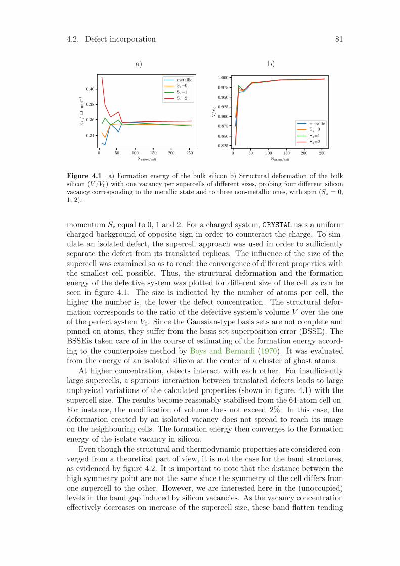
4.2. Defect incorporation 81
a) b)
0 50 100 150 200 250
Natom/cell
0.34
0.36
0.38
0.40
Ef
/kJ·m
ol−
1metallicSz=0
Sz=1
Sz=2
0 50 100 150 200 250
Natom/cell
0.825
0.850
0.875
0.900
0.925
0.950
0.975
1.000
V/V
0
metallicSz=0
Sz=1
Sz=2
Figure 4.1 a) Formation energy of the bulk silicon b) Structural deformation of the bulksilicon (V /V0) with one vacancy per supercells of different sizes, probing four different siliconvacancy corresponding to the metallic state and to three non-metallic ones, with spin (Sz = 0,1, 2).
momentum Sz equal to 0, 1 and 2. For a charged system, CRYSTAL uses a uniformcharged background of opposite sign in order to counteract the charge. To sim-ulate an isolated defect, the supercell approach was used in order to sufficientlyseparate the defect from its translated replicas. The influence of the size of thesupercell was examined so as to reach the convergence of different properties withthe smallest cell possible. Thus, the structural deformation and the formationenergy of the defective system was plotted for different size of the cell as can beseen in figure 4.1. The size is indicated by the number of atoms per cell, thehigher the number is, the lower the defect concentration. The structural defor-mation corresponds to the ratio of the defective system’s volume V over the oneof the perfect system V0. Since the Gaussian-type basis sets are not complete andpinned on atoms, they suffer from the basis set superposition error (BSSE). TheBSSEis taken care of in the course of estimating of the formation energy accord-ing to the counterpoise method by Boys and Bernardi (1970). It was evaluatedfrom the energy of an isolated silicon at the center of a cluster of ghost atoms.
At higher concentration, defects interact with each other. For insufficientlylarge supercells, a spurious interaction between translated defects leads to largeunphysical variations of the calculated properties (shown in figure. 4.1) with thesupercell size. The results become reasonably stabilised from the 64-atom cell on.For instance, the modification of volume does not exceed 2%. In this case, thedeformation created by an isolated vacancy does not spread to reach its imageon the neighbouring cells. The formation energy then converges to the formationenergy of the isolate vacancy in silicon.
Even though the structural and thermodynamic properties are considered con-verged from a theoretical part of view, it is not the case for the band structures,as evidenced by figure 4.2. It is important to note that the distance between thehigh symmetry point are not the same since the symmetry of the cell differs fromone supercell to the other. However, we are interested here in the (unoccupied)levels in the band gap induced by silicon vacancies. As the vacancy concentrationeffectively decreases on increase of the supercell size, these band flatten tending
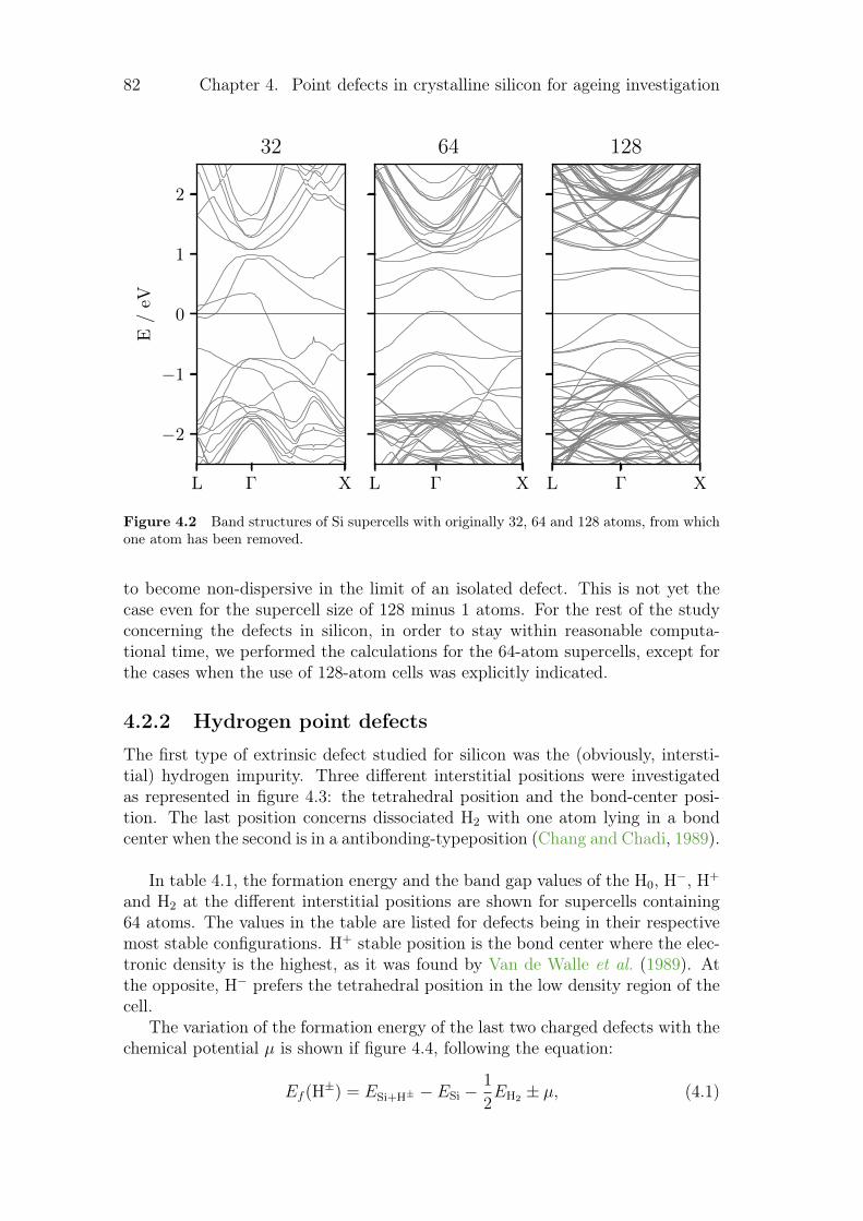
82 Chapter 4. Point defects in crystalline silicon for ageing investigation
L Γ X
−2
−1
0
1
2
E/
eV32
L Γ X
64
L Γ X
128
Figure 4.2 Band structures of Si supercells with originally 32, 64 and 128 atoms, from whichone atom has been removed.
to become non-dispersive in the limit of an isolated defect. This is not yet thecase even for the supercell size of 128 minus 1 atoms. For the rest of the studyconcerning the defects in silicon, in order to stay within reasonable computa-tional time, we performed the calculations for the 64-atom supercells, except forthe cases when the use of 128-atom cells was explicitly indicated.
4.2.2 Hydrogen point defects
The first type of extrinsic defect studied for silicon was the (obviously, intersti-tial) hydrogen impurity. Three different interstitial positions were investigatedas represented in figure 4.3: the tetrahedral position and the bond-center posi-tion. The last position concerns dissociated H2 with one atom lying in a bondcenter when the second is in a antibonding-typeposition (Chang and Chadi, 1989).
In table 4.1, the formation energy and the band gap values of the H0, H−, H+
and H2 at the different interstitial positions are shown for supercells containing64 atoms. The values in the table are listed for defects being in their respectivemost stable configurations. H+ stable position is the bond center where the elec-tronic density is the highest, as it was found by Van de Walle et al. (1989). Atthe opposite, H− prefers the tetrahedral position in the low density region of thecell.
The variation of the formation energy of the last two charged defects with thechemical potential µ is shown if figure 4.4, following the equation:
Ef (H±) = ESi+H± − ESi −
1
2EH2 ± µ, (4.1)
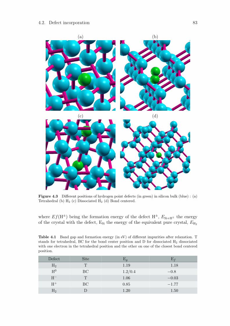
4.2. Defect incorporation 83
(a) (b)
(c) (d)
Figure 4.3 Different positions of hydrogen point defects (in green) in silicon bulk (blue) : (a)Tetrahedral (b) H2 (c) Dissociated H2 (d) Bond centered.
where Ef(H±) being the formation energy of the defect H±, ESi+H± the energyof the crystal with the defect, ESi the energy of the equivalent pure crystal, EH2
Table 4.1 Band gap and formation energy (in eV) of different impurities after relaxation. Tstands for tetrahedral, BC for the bond center position and D for dissociated H2 dissociatedwith one electron in the tetrahedral position and the other on one of the closest bond centeredposition.
Defect Site Eg EfH2 T 1.19 1.18
H0 BC 1.2/0.4 −0.8
H− T 1.06 −0.03
H+ BC 0.85 −1.77
H2 D 1.20 1.50
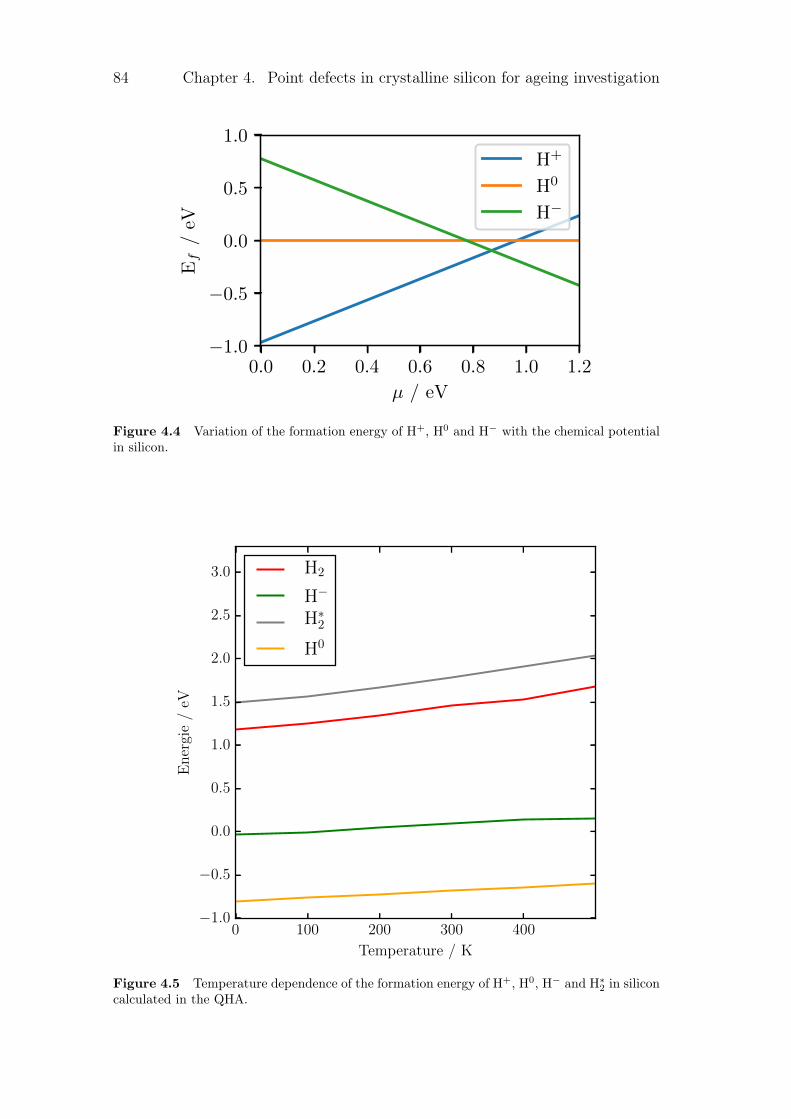
84 Chapter 4. Point defects in crystalline silicon for ageing investigation
0.0 0.2 0.4 0.6 0.8 1.0 1.2
µ / eV
−1.0
−0.5
0.0
0.5
1.0
Ef
/eV
H+
H0
H−
Figure 4.4 Variation of the formation energy of H+, H0 and H− with the chemical potentialin silicon.
0 100 200 300 400
Temperature / K
−1.0
−0.5
0.0
0.5
1.0
1.5
2.0
2.5
3.0
En
ergi
e/
eV
H2
H−
H∗2
H0
Figure 4.5 Temperature dependence of the formation energy of H+, H0, H− and H∗2 in siliconcalculated in the QHA.
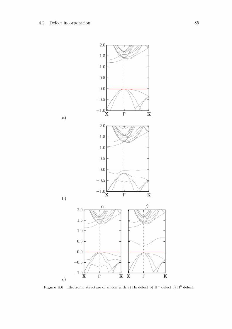
4.2. Defect incorporation 85
a)X Γ K
−1.0
−0.5
0.0
0.5
1.0
1.5
2.0
b)X Γ K
−1.0
−0.5
0.0
0.5
1.0
1.5
2.0
c)X Γ K
−1.0
−0.5
0.0
0.5
1.0
1.5
2.0α
X Γ K
β
Figure 4.6 Electronic structure of silicon with a) H2 defect b) H− defect c) H0 defect.
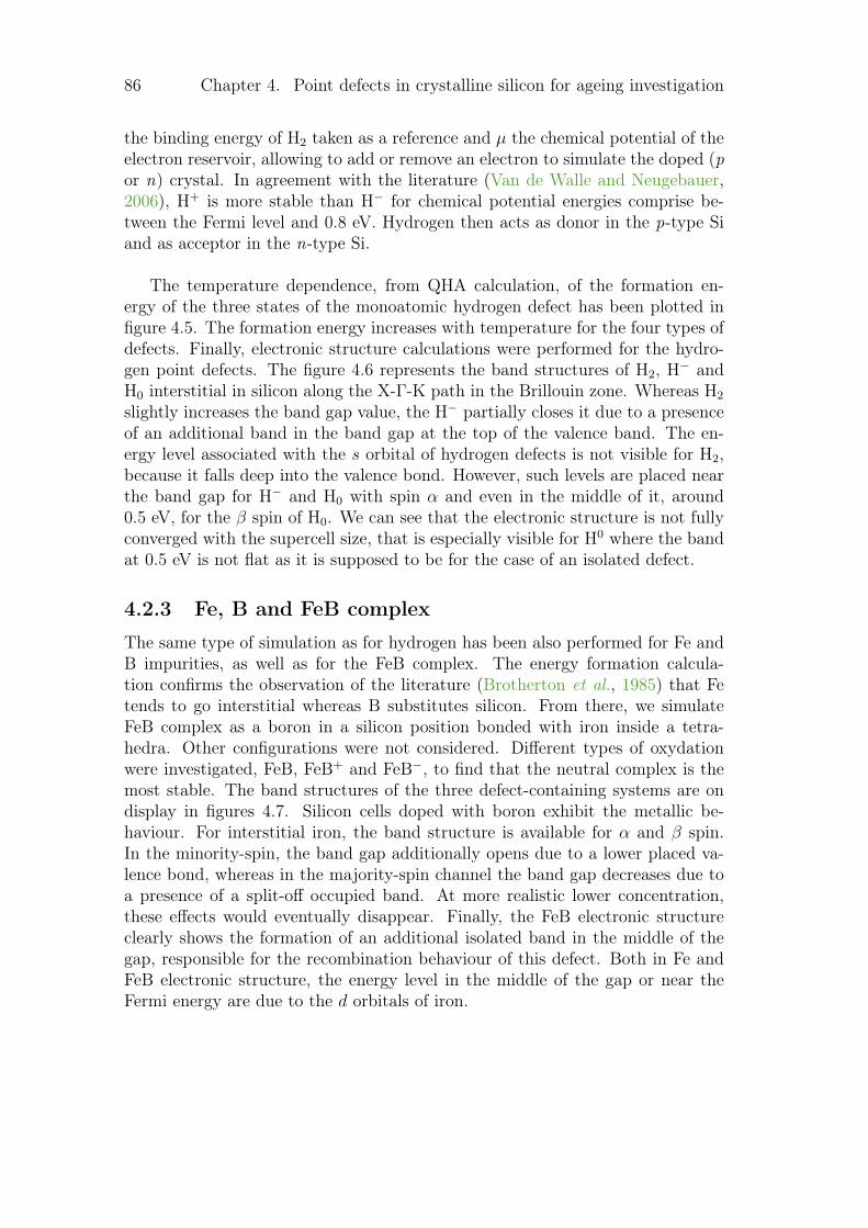
86 Chapter 4. Point defects in crystalline silicon for ageing investigation
the binding energy of H2 taken as a reference and µ the chemical potential of theelectron reservoir, allowing to add or remove an electron to simulate the doped (por n) crystal. In agreement with the literature (Van de Walle and Neugebauer,2006), H+ is more stable than H− for chemical potential energies comprise be-tween the Fermi level and 0.8 eV. Hydrogen then acts as donor in the p-type Siand as acceptor in the n-type Si.
The temperature dependence, from QHA calculation, of the formation en-ergy of the three states of the monoatomic hydrogen defect has been plotted infigure 4.5. The formation energy increases with temperature for the four types ofdefects. Finally, electronic structure calculations were performed for the hydro-gen point defects. The figure 4.6 represents the band structures of H2, H− andH0 interstitial in silicon along the X-Γ-K path in the Brillouin zone. Whereas H2
slightly increases the band gap value, the H− partially closes it due to a presenceof an additional band in the band gap at the top of the valence band. The en-ergy level associated with the s orbital of hydrogen defects is not visible for H2,because it falls deep into the valence bond. However, such levels are placed nearthe band gap for H− and H0 with spin α and even in the middle of it, around0.5 eV, for the β spin of H0. We can see that the electronic structure is not fullyconverged with the supercell size, that is especially visible for H0 where the bandat 0.5 eV is not flat as it is supposed to be for the case of an isolated defect.
4.2.3 Fe, B and FeB complex
The same type of simulation as for hydrogen has been also performed for Fe andB impurities, as well as for the FeB complex. The energy formation calcula-tion confirms the observation of the literature (Brotherton et al., 1985) that Fetends to go interstitial whereas B substitutes silicon. From there, we simulateFeB complex as a boron in a silicon position bonded with iron inside a tetra-hedra. Other configurations were not considered. Different types of oxydationwere investigated, FeB, FeB+ and FeB−, to find that the neutral complex is themost stable. The band structures of the three defect-containing systems are ondisplay in figures 4.7. Silicon cells doped with boron exhibit the metallic be-haviour. For interstitial iron, the band structure is available for α and β spin.In the minority-spin, the band gap additionally opens due to a lower placed va-lence bond, whereas in the majority-spin channel the band gap decreases due toa presence of a split-off occupied band. At more realistic lower concentration,these effects would eventually disappear. Finally, the FeB electronic structureclearly shows the formation of an additional isolated band in the middle of thegap, responsible for the recombination behaviour of this defect. Both in Fe andFeB electronic structure, the energy level in the middle of the gap or near theFermi energy are due to the d orbitals of iron.
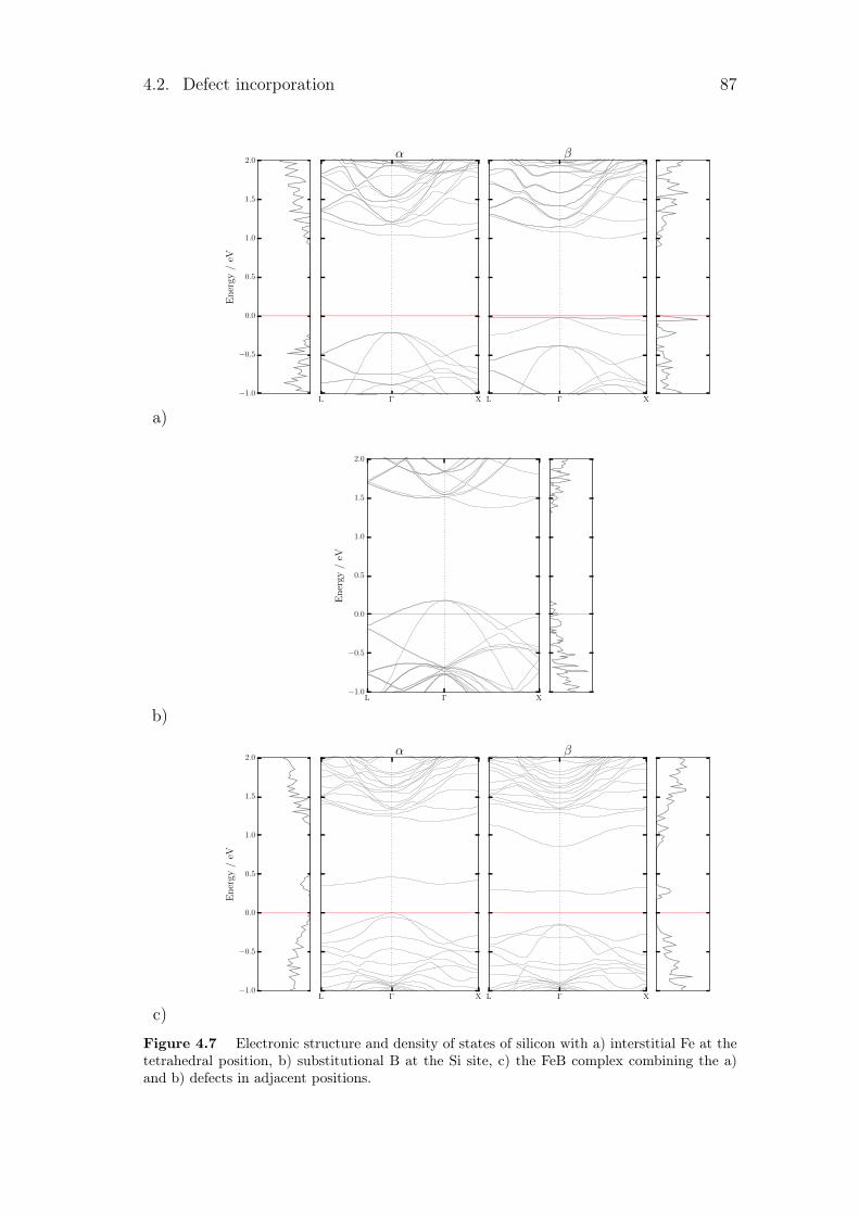
4.2. Defect incorporation 87
a)−1.0
−0.5
0.0
0.5
1.0
1.5
2.0
En
ergy
/eV
L Γ X
α
L Γ X
β
b)L Γ X
−1.0
−0.5
0.0
0.5
1.0
1.5
2.0
En
ergy
/eV
c)−1.0
−0.5
0.0
0.5
1.0
1.5
2.0
En
ergy
/eV
L Γ X
α
L Γ X
β
Figure 4.7 Electronic structure and density of states of silicon with a) interstitial Fe at thetetrahedral position, b) substitutional B at the Si site, c) the FeB complex combining the a)and b) defects in adjacent positions.
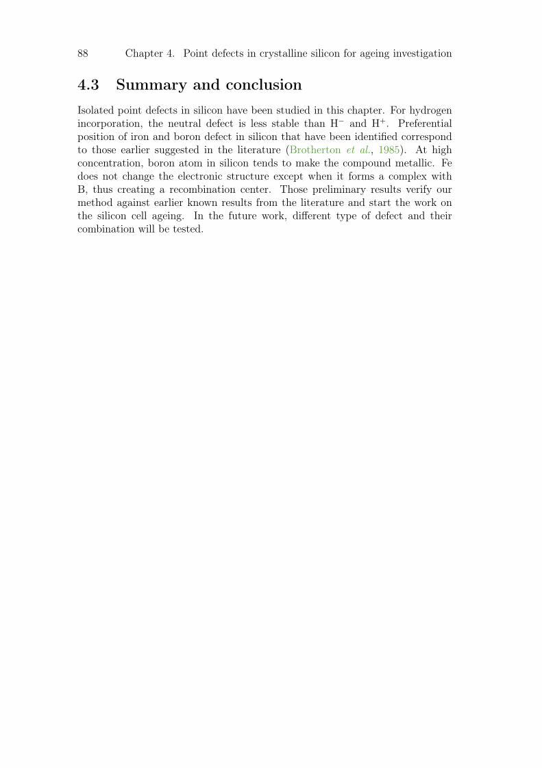
88 Chapter 4. Point defects in crystalline silicon for ageing investigation
4.3 Summary and conclusionIsolated point defects in silicon have been studied in this chapter. For hydrogenincorporation, the neutral defect is less stable than H− and H+. Preferentialposition of iron and boron defect in silicon that have been identified correspondto those earlier suggested in the literature (Brotherton et al., 1985). At highconcentration, boron atom in silicon tends to make the compound metallic. Fedoes not change the electronic structure except when it forms a complex withB, thus creating a recombination center. Those preliminary results verify ourmethod against earlier known results from the literature and start the work onthe silicon cell ageing. In the future work, different type of defect and theircombination will be tested.
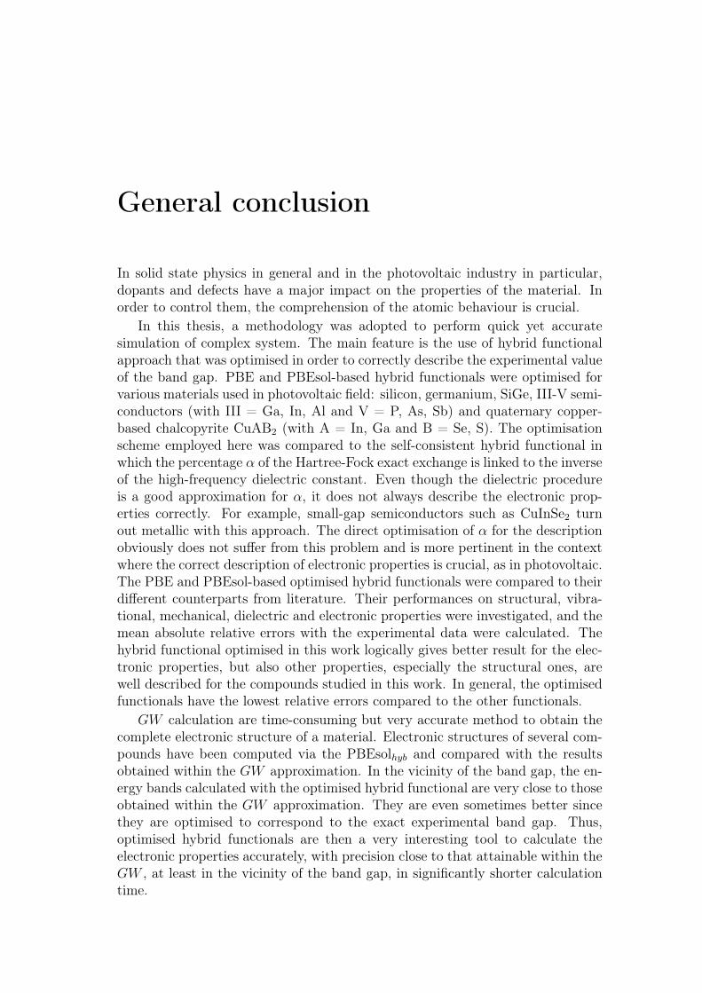
General conclusion
In solid state physics in general and in the photovoltaic industry in particular,dopants and defects have a major impact on the properties of the material. Inorder to control them, the comprehension of the atomic behaviour is crucial.
In this thesis, a methodology was adopted to perform quick yet accuratesimulation of complex system. The main feature is the use of hybrid functionalapproach that was optimised in order to correctly describe the experimental valueof the band gap. PBE and PBEsol-based hybrid functionals were optimised forvarious materials used in photovoltaic field: silicon, germanium, SiGe, III-V semi-conductors (with III = Ga, In, Al and V = P, As, Sb) and quaternary copper-based chalcopyrite CuAB2 (with A = In, Ga and B = Se, S). The optimisationscheme employed here was compared to the self-consistent hybrid functional inwhich the percentage α of the Hartree-Fock exact exchange is linked to the inverseof the high-frequency dielectric constant. Even though the dielectric procedureis a good approximation for α, it does not always describe the electronic prop-erties correctly. For example, small-gap semiconductors such as CuInSe2 turnout metallic with this approach. The direct optimisation of α for the descriptionobviously does not suffer from this problem and is more pertinent in the contextwhere the correct description of electronic properties is crucial, as in photovoltaic.The PBE and PBEsol-based optimised hybrid functionals were compared to theirdifferent counterparts from literature. Their performances on structural, vibra-tional, mechanical, dielectric and electronic properties were investigated, and themean absolute relative errors with the experimental data were calculated. Thehybrid functional optimised in this work logically gives better result for the elec-tronic properties, but also other properties, especially the structural ones, arewell described for the compounds studied in this work. In general, the optimisedfunctionals have the lowest relative errors compared to the other functionals.
GW calculation are time-consuming but very accurate method to obtain thecomplete electronic structure of a material. Electronic structures of several com-pounds have been computed via the PBEsolhyb and compared with the resultsobtained within the GW approximation. In the vicinity of the band gap, the en-ergy bands calculated with the optimised hybrid functional are very close to thoseobtained within the GW approximation. They are even sometimes better sincethey are optimised to correspond to the exact experimental band gap. Thus,optimised hybrid functionals are then a very interesting tool to calculate theelectronic properties accurately, with precision close to that attainable within theGW , at least in the vicinity of the band gap, in significantly shorter calculationtime.
90 General conclusion
The effect of temperature was then tested with the quasi-harmonic approxi-mation. The variation of the thermal expansion, the heat capacity and the bandgap with the temperature show different behaviour compared to experimentaldata. The first two properties are well described with the temperature variation,but the band gap dependence does not correspond to experimental trends. Theinclusion of the electron-phonon coupling in the calculations might be necessaryin order to provide the essential correction. Nevertheless, the choice of particularfunctional does not seem to be very important for estimating the temperaturedependence of properties, the resulting behaviour comes out about the same.For thermodynamic study, the optimised hybrid functional is then not markedlybetter than the other functionals.
Finally, the influence of the choice of functional on the electrical conductivitywas studied. Once again, thanks to the correct description of the band gap,optimised hybrid functional give the most accurate result. The larger the fractionof the HF-exact exchange, the higher the calculated electrical conductivity. Atthis point the methodology have been validated for pure material and ready touse on more complex systems.
The first complex systems investigated were chalcopyrite compounds. One ofthe key features of CIGSSe is the control of their composition that leads to atunability of different properties, such as the lattice parameter or the band gap.This feature makes chalcopyrite system promising candidates for applications intandem cells. In this work, two separate studies on CIGSSe were performedIn the first study, the influence of composition for the penternary chalcopyriteCuInxGa1−x(SeyS1−y)2 on different properties was investigated. A complete map-ping of the lattice parameters, band gap and formation energy with the two con-centrations x and y was done. The variation of the first properties was practicallylinear with the concentration and was in agreement with the experimental data.The “optimal” band gap values of 1.5 – 1.7 eV are accessible for higher concen-tration of indium than gallium. However, the lattice mismatch with the latticeparameter of silicon in this range of concentrations becomes more important.Even if the lattice mismatch is low, the epitaxy of chalcopyrite on top of a siliconwafer might be difficult. The silicon lattice parameter corresponds to that ofchalcopyrite with higher concentration of gallium and sulphur. In all the compo-sitions studied, the system stays in the chalcopyrite symmetry and the energiesof formation are negative, thus the system is thermodynamically stable and nosecondary phases appear.
In the second study, alkali incorporation by means of cation substitution wereperformed by a similar method. As alkali post-deposition treatment has beenshown in the last five years to be able to importantly increase the efficiency ofCIGSSe solar cells, the understanding of the origin of this effect is of great inter-est. In a few theoretical works so far done on the simulation of point defects, thecopper site was identified as the most favorable incorporation site. In this work,we substituted copper by alkali metal for a broad range of concentration, in orderto grasp their influence of these dopants on the bulk. The first observation isthat alkali metal atoms increase the volume of the cell with an expansion of thelattice parameter a but a contraction of c. However, the system goes from the
91
P 4 symmetry at lowest concentration to C2/c for the highest one, except for thecase of doping with lithium and most of the cases concerning sodium; however,this might be due to an intrinsic issue of the method. This deformation is purelydue to the local deformation of the tetrahedra around the substituted atoms.The calculation of electronic properties were then performed. The Mulliken pop-ulation analysis shows that the different compounds become more ionic with theincorporation of alkali As for the band gap, it increases with the concentration ofalkali metal. That is not a good news for gallium-based ternary chalcopyrites thathave band gap already larger than the target value, however might be useful forindium-based chalcopyrites to reach the target value. Different energy relationswere then calculated corresponding to various chemical reactions. The main con-clusion is that the alkali metals incorporation is not easy in chalcopyrite. Evenif Li, Na and K have substitution energy lower than 2 eV and hence much lowerthan Rb and Cs whose substitution energy is around 4 – 5 eV, all these energiesare positive, and the substitution reaction is not spontaneous. Moreover, exceptfor the lithium, thermodynamically, the substitution of the Cu by a alkali met-als will lead to the appearance of the secondary phases whatever the consideredmechanisms.
Finally, the second complex system studied was silicon with various pointdefects. In the context of a global project working on the ageing of silicon so-lar cell, the light and elevated temperature induced degradation (LeTID) mightbe the consequence of atomic effect linked to hydrogen trapped in the bulk andinteracting with defect (iron) or dopant (boron). In this thesis, we performedpreliminary calculation of H, Fe, B point defects and FeB complex. Even thoughthese defects are well known in the literature, they served excellent benchmarksto test and validate the calculation method. The most stable position of thedifferent charge states of the point defect correspond to the knowledge from theliterature. Now that the simulation of simple isolated defects have been demon-strated to be reliable, the combination of defects can be probed, and the wayopened to simulations of the defects’ interaction among themselves and e.g. withdislocations.

Bibliography
Abou-Ras, D., S. Wagner, B. J. Stanbery, H.-W. Schock et al. (2017). Innova-tion highway: Breakthrough milestones and key developments in chalcopyritephotovoltaics from a retrospective viewpoint. Thin Solid Films 633, 2.
Abrahams, S. C. and J. L. Bernstein (1974). Piezoelectric nonlinear op-tic CuGaSe2 and CdGeAs2: Crystal structure, chalcopyrite microhard-ness, and sublattice distortion. The Journal of Chemical Physics 61(3),1140. URL http://scitation.aip.org/content/aip/journal/jcp/61/3/10.1063/1.1681987.
Adachi, S. (1985). GaAs, AlAs, and AlxGa1-xAs: Material parameters for use inresearch and device applications. Journal of Applied Physics 58(3), R1. URLhttp://aip.scitation.org/doi/10.1063/1.336070.
Adamo, C. and V. Barone (1999). Toward reliable density functional methodswithout adjustable parameters: The PBE0 model. The Journal of ChemicalPhysics 110(13), 6158. URL http://aip.scitation.org/doi/10.1063/1.478522.
Aguilera, I., J. Vidal, P. Wahnòn, L. Reining et al. (2011). First-principles studyof the band structure and optical absorption of CuGaS2. Physical Review B84(8). URL https://link.aps.org/doi/10.1103/PhysRevB.84.085145.
Alkauskas, A., P. Broqvist, F. Devynck and A. Pasquarello (2008). Band Offsetsat Semiconductor-Oxide Interfaces from Hybrid Density-Functional Calcula-tions. Physical Review Letters 101(10). URL https://link.aps.org/doi/10.1103/PhysRevLett.101.106802.
Alkauskas, A., P. Broqvist and A. Pasquarello (2011). Defect levels throughhybrid density functionals: Insights and applications. physica status solidi (b)248(4), 775. URL http://doi.wiley.com/10.1002/pssb.201046195.
Alkauskas, A. and A. Pasquarello (2011). Band-edge problem in the theoreticaldetermination of defect energy levels: The O vacancy in ZnO as a benchmarkcase. Physical Review B 84(12). URL https://link.aps.org/doi/10.1103/PhysRevB.84.125206.
Allen, P. (1996). Boltzmann theory and resistivity of metals. Kluwer InternationalSeries in Engineering and Computer Science 219–250.
94 Bibliography
Allen, P. B. and V. Heine (1976). Theory of the temperature dependence ofelectronic band structures. Journal of Physics C: Solid State Physics 9(12),2305. URL https://doi.org/10.1088%2F0022-3719%2F9%2F12%2F013.
Alonso, M. I. and K. Winer (1989). Raman spectra of c–Si1−xGex alloys. Phys-ical Review B 39(14), 10056. URL https://link.aps.org/doi/10.1103/PhysRevB.39.10056.
Aryasetiawan, F. and O. Gunnarsson (1998). The GW method. Reports onProgress in Physics 61(3), 237. URL https://doi.org/10.1088/0034-4885/61/3/002.
Aspnes and Studna (1972). Direct observation of the E0 and E0+δ0 transition insilion. Solid State Communications 11(10), 1375.
Azuhata, T., T. Sota and K. Suzuki (1995). Second-order Raman spectra andlattice dynamics in AlAs. Journal of Physics: Condensed Matter 7(9), 1949.URL https://doi.org/10.1088%2F0953-8984%2F7%2F9%2F018.
Baars, J. and W. H. Koschel (1972). Dielectric dispersion of CuGaS2 by infraredreflectivity analysis. Solid State Communications 11(11), 1513. URL http://www.sciencedirect.com/science/article/pii/003810987290511X.
Bär, M., W. Bohne, J. Röhrich, E. Strub et al. (2004). Determination of theband gap depth profile of the penternary Cu(In1−xGax)(SySe1−y)2 chalcopyritefrom its composition gradient. Journal of Applied Physics 96(7), 3857. URLhttp://aip.scitation.org/doi/10.1063/1.1786340.
Barker, A. S. (1968). Dielectric Dispersion and Phonon Line Shape in GalliumPhosphide. Physical Review 165(3), 917. URL https://link.aps.org/doi/10.1103/PhysRev.165.917.
Becke, A. D. (1993a). Density functional thermochemistry. III. The role of exactexchange. The Journal of Chemical Physics 98(7), 5648. URL http://aip.scitation.org/doi/10.1063/1.464913.
Becke, A. D. (1993b). A new mixing of Hartree–Fock and local density functionaltheories. The Journal of Chemical Physics 98(2), 1372. URL http://aip.scitation.org/doi/10.1063/1.464304.
Beer, S., J. Jackovitz, D. Feldman and J. Parker (1968). Raman and infraredactive modes of aluminium phosphide. Physics Letters A 26(7), 331. URLhttps://linkinghub.elsevier.com/retrieve/pii/0375960168906804.
Bettini, M. and W. B. Holzapfel (1975). Grüneisen parameters of τphonons in CdSiP2, CuAlS2 and CuGaS2. Solid State Communications16(1), 27. URL http://www.sciencedirect.com/science/article/pii/0038109875907814.
Bibliography 95
Betzinger, M. (2007). Efficient Implementation of the Non–Local ExchangePotential within the FLAPW Method. Ph.D. thesis, Diplomarbeit, RWTHAachen, Institut für Festkörperphysik, Forschungszentrum Jülich.
Biernacki, S. and M. Scheffler (1989). Negative thermal expansion of diamondand zinc-blende semiconductors. Physical Review Letters 63(3), 290. URLhttps://link.aps.org/doi/10.1103/PhysRevLett.63.290.
Birch, F. (1947). Finite Elastic Strain of Cubic Crystals. Physical Review 71(11),809. URL https://link.aps.org/doi/10.1103/PhysRev.71.809.
Bludau, W., A. Onton and W. Heinke (1974). Temperature dependence of theband gap of silicon. Journal of Applied Physics 45(4), 1846. URL http://aip.scitation.org/doi/10.1063/1.1663501.
Bodnar, I. V., B. V. Korzun and A. I. Lukomskii (1981). Composition dependenceof the band gap of CuInS2xSe2(1−x). physica status solidi (b) 105(2), K143. URLhttp://onlinelibrary.wiley.com/doi/abs/10.1002/pssb.2221050259.
Bodnar, I. V. and A. I. Lukomskii (1986). The concentration dependence ofthe band gap CuGaxIn1−xS2 and AgGaxIn1−xS2 solid solutions. physica statussolidi (a) 98(2), K165. URL http://onlinelibrary.wiley.com/doi/abs/10.1002/pssa.2210980255.
Bodnar, I. V. and N. S. Orlova (1983). X-ray study of the thermal expansionin CuAlS2, CuGaS2, and CuInS2 compounds over the temperature range from90 to 650 K. Physica Status Solidi (a) 78(1), K59. URL http://doi.wiley.com/10.1002/pssa.2210780155.
Boehnke, U. and H. Neumann (1992). Cu1−xLixInSe2. Journal of Alloys andCompounds 190(1).
Bolef, D. I. and M. Menes (1960). Elastic Constants of Single–Crystal Alu-minum Antimonide. Journal of Applied Physics 31(8), 1426. URL http://aip.scitation.org/doi/10.1063/1.1735857.
Born, M. and R. Oppenheimer (1927). Zur Quantentheorie der Molekeln. An-nalen der Physik 389(20), 457. URL https://onlinelibrary.wiley.com/doi/abs/10.1002/andp.19273892002.
Boyle, W. F. and R. J. Sladek (1975). Elastic constants and lattice anharmonicityof GaSb and GaP from ultrasonic-velocity measurements between 4.2 and 300K. Physical Review B 11(8), 2933. URL https://link.aps.org/doi/10.1103/PhysRevB.11.2933.
Boys, S. (1950). Electronic wave functions. I. A general method of calculation forthe stationary states of any molecular system. Proceeding of the Royal Societyof London 200.
96 Bibliography
Boys, S. and F. Bernardi (1970). The calculation of small molecular interactionsby the differences of separate total energies. Some procedures with reducederrors. Molecular Physics 19(4), 553. URL http://www.tandfonline.com/doi/full/10.1080/00268977000101561.
Broqvist, P., A. Alkauskas and A. Pasquarello (2008). Defect levels of danglingbonds in silicon and germanium through hybrid functionals. Physical ReviewB 78(7). URL https://link.aps.org/doi/10.1103/PhysRevB.78.075203.
Brotherton, S. D., P. Bradley and A. Gill (1985). Iron and the iron-boroncomplex in silicon. Journal of Applied Physics 57(6), 1941. URL http://aip.scitation.org/doi/10.1063/1.335468.
Cardona, M., F. H. Pollak and K. L. Shaklee (1966). Electroreflectance in AlSb:Observation of the Direct Band Edge. Physical Review Letters 16(15), 644.URL https://link.aps.org/doi/10.1103/PhysRevLett.16.644.
Carles, R., N. Saint-Cricq, J. B. Renucci, M. A. Renucci et al. (1980). Second-order Raman scattering in InAs. Physical Review B 22(10), 4804. URL https://link.aps.org/doi/10.1103/PhysRevB.22.4804.
Carr, J. A. and S. Chaudhary (2013). The identification, characterization andmitigation of defect states in organic photovoltaic devices: a review and out-look. Energy & Environmental Science 6(12), 3414. URL http://xlink.rsc.org/?DOI=c3ee41860j.
Chang, K. J. and D. J. Chadi (1989). Hydrogen bonding and diffusion in crys-talline silicon. Physical Review B 40(17), 11644. URL https://link.aps.org/doi/10.1103/PhysRevB.40.11644.
Chen, D., P. G. Hamer, M. Kim, T. H. Fung et al. (2018). Hydrogen in-duced degradation: A possible mechanism for light- and elevated temperature-induced degradation in n-type silicon. Solar Energy Materials and SolarCells 185, 174. URL https://linkinghub.elsevier.com/retrieve/pii/S0927024818302617.
Chirilă, A., P. Reinhard, F. Pianezzi, P. Bloesch et al. (2013). Potassium-inducedsurface modification of Cu(In,Ga)Se2 thin films for high-efficiency solar cells.Nature Materials 12(12), 1107.
Cho, D.-H., K.-S. Lee, Y.-D. Chung, J.-H. Kim et al. (2012). Electronic effect ofNa on Cu(In,Ga)Se2 solar cells. Appl. Phys. Lett. 5.
Cojocaru-Mirédin, O., P.-P. Choi, D. Abou-Ras, S. S. Schmidt et al. (2011). Char-acterization of Grain Boundaries in Cu(In,Ga)Se2 Films Using Atom-ProbeTomography. IEEE Journal of Photovoltaics 1(2), 207.
Cojocaru-Mirédin, O., T. Schwarz, P.-P. Choi, M. Herbig et al. (2013). Atomprobe tomography studies on the Cu(In,Ga)Se2 grain boundaries. Journal ofVisualized Experiments : JoVE 74. URL https://www.ncbi.nlm.nih.gov/pmc/articles/PMC3667468/.
Bibliography 97
Conesa, J. C. (2012). Modeling with Hybrid Density Functional Theory theElectronic Band Alignment at the Zinc Oxide–Anatase Interface. The Journalof Physical Chemistry C 116(35), 18884. URL http://pubs.acs.org/doi/10.1021/jp306160c.
Contreras, M. A., B. Egaas, P. Dippo, J. Webb et al. (1997). On the role of naand modifications to Cu(In,Ga)Se2 absorber materials using thin-MF (M= Na,K, Cs) precursor layers [solar cells]. In Conference Record of the Twenty SixthIEEE Photovoltaic Specialists Conference-1997 , 359–362. IEEE.
Corruccini, R. J. and J. J. Gniewek (1960). Specific heats and enthalpies of tech-nical solids at low temperatures. A compilation from the literature. TechnicalReport NBS-Mon-21, National Bureau of Standards, Washington, D.C. URLhttps://www.osti.gov/biblio/4803576.
Cottam, R. I. and G. A. Saunders (1973). The elastic constants ofGaAs from 2 K to 320 K. Journal of Physics C: Solid State Physics6(13), 2105. URL http://stacks.iop.org/0022-3719/6/i=13/a=011?key=crossref.f69af4617f3239c6ea359f866ce8a29d.
Coughlan, C., M. Ibáñez, O. Dobrozhan, A. Singh et al. (2017). Compoundcopper chalcogenide nanocrystals. Chemical Reviews 117(9), 5865. URL http://pubs.acs.org/doi/10.1021/acs.chemrev.6b00376.
CRYSTAL17 (2019). CRYSTAL - basis sets library. URL http://www.crystal.unito.it/basis-sets.php.
Deák, P., A. Gali, A. Sólyom, A. Buruzs et al. (2005). Electronic structure ofboron-interstitial clusters in silicon. Journal of Physics: Condensed Matter17(22), S2141. URL http://stacks.iop.org/0953-8984/17/i=22/a=001?key=crossref.c6b31286fe557d1278163f8e2c06d3ce.
Desai, P. D. (1986). Thermodynamic Properties of Iron and Silicon. Jour-nal of Physical and Chemical Reference Data 15(3), 967. URL http://aip.scitation.org/doi/10.1063/1.555761.
Deus, P., H. Neumann, G. Kühn and B. Hinze (1983a). Low-temperature thermalexpansion in CuInSe2. Physica Status Solidi (a) 80(1), 205. URL http://doi.wiley.com/10.1002/pssa.2210800122.
Deus, P., U. Voland and H. A. Schneider (1983b). Thermal expansion of GaPwithin 20 to 300 K. Physica Status Solidi (a) 80(1), K29. URL http://doi.wiley.com/10.1002/pssa.2210800152.
Dirac, P. A. M. (1930). Note on Exchange Phenomena in the ThomasAtom. Mathematical Proceedings of the Cambridge Philosophical Soci-ety 26(03), 376. URL http://www.journals.cambridge.org/abstract_S0305004100016108.
98 Bibliography
Dismukes, J. P., L. Ekstrom and R. J. Paff (1964). Lattice Parameter and Densityin Germanium-Silicon Alloys. Journal of Physicsal Chemistry 437(10), 3021.
Dovesi, R., B. Civalleri, R. Orlando, C. Roetti et al. (2005). Ab initio quantumsimulation in solid state chemistry. Reviews in computational chemistry 21, 1.
Dovesi, R., A. Erba, R. Orlando, C. M. Zicovich-Wilson et al. (2018). Quantum-mechanical condensed matter simulations with CRYSTAL. Wiley Interdisci-plinary Reviews: Computational Molecular Science 8(4).
Dovesi, R., E. Ermondi, E. Ferrero, C. Pisani et al. (1983). Hartree-Fock studyof lithium hydride with the use of a polarizable basis set. Phys. Rev. B 29,3591. URL https://doi.org/10.1103/PhysRevB.29.3591.
Dovesi, R., C. Roetti, C. Freyria Fava and V. Prencipe, M.and Saunders (1991).On the elastic properties of lithium, sodium an potassium oxide. An ab initiostudy. Chem. Phys. 156, 11.
Dziedzic, J., Q. Hill and C.-K. Skylaris (2013). Linear-scaling calculation ofHartree-Fock exchange energy with non-orthogonal generalised Wannier func-tions. The Journal of Chemical Physics 139(21), 214103. URL http://aip.scitation.org/doi/10.1063/1.4832338.
Eid, J., H. Liang, I. Gereige, S. Lee et al. (2015). Combinatorial study of NaFaddition in CIGSe films for high efficiency solar cells. Progress in Photovoltaics:Research and Applications 23(3), 269.
Eifler, A., V. Riede, J. Brückner, S. Weise et al. (2000). Band Gap Energiesand Lattice Vibrations of the Lithium Ternary Compounds LiInSe2 , LiInS2 ,LiGaSe2 and LiGaS2. Japanese Journal of Applied Physics 39(S1), 279. URLhttp://stacks.iop.org/1347-4065/39/279.
Erba, A. (2014). On combining temperature and pressure effects on structuralproperties of crystals with standard ab initio techniques. The Journal ofChemical Physics 141(12), 124115. URL http://aip.scitation.org/doi/10.1063/1.4896228.
Erba, A. (2017). Self-consistent hybrid functionals for solids: a fully-automated implementation. Journal of Physics: Condensed Matter 29(31),314001. URL http://stacks.iop.org/0953-8984/29/i=31/a=314001?key=crossref.688c4f145cedf8f27dc556a5cff87ee4.
Faghaninia, A. (2016). Theory of Carrier Transport From First Principles: Ap-plications in Photovoltaic and Thermoelectric Materials. Ph.D. thesis, Wash-ington University.
Faghaninia, A., J. W. Ager and C. S. Lo (2015). Ab initio electronic transportmodel with explicit solution to the linearized Boltzmann transport equation.Phys. Rev. B 91(23).

Bibliography 99
Faghaninia, A., G. Yu, U. Aydemir, M. Wood et al. (2017). A computationalassessment of the electronic, thermoelectric, and defect properties of bournonite(CuPbSbS3) and related substitutions. Physical Chemistry Chemical Physics19(9), 6743.
Fang, Z. M., K. Y. Ma, D. H. Jaw, R. M. Cohen et al. (1990). Photolumines-cence of InSb, InAs, and InAsSb grown by organometallic vapor phase epitaxy.Journal of Applied Physics 67(11), 7034. URL http://aip.scitation.org/doi/10.1063/1.345050.
Faulkner, R. A. (1969). Higher donor excited states for prolate-spheroid conduc-tion bands: A reevaluation of silicon and germanium. Physical Review 184(3),713. URL https://link.aps.org/doi/10.1103/PhysRev.184.713.
Feng, K., D. Mei, L. Bai, Z. Lin et al. (2012). Synthesis, structure,physical properties, and electronic structure of KGaSe2. Solid State Sci-ences 14(8), 1152. URL https://linkinghub.elsevier.com/retrieve/pii/S1293255812001914.
Ferrero, M., M. Rérat, R. Orlando and R. Dovesi (2008). Coupled perturbedHartree-Fock for periodic systems: The role of symmetry and related com-putational aspects. The Journal of Chemical Physics 128(1), 014110. URLhttp://aip.scitation.org/doi/10.1063/1.2817596.
Fine, M. E. (1955). Elastic Constants of Germanium between 1.7 and 80 K.Journal of Applied Physics 26(7), 862. URL http://aip.scitation.org/doi/10.1063/1.1722110.
Fock, V. (1930). Näherungsmethode zur Lösung des quantenmechanischenMehrkörperproblems. Zeitschrift für Physik 61(1–2), 126. URL http://dx.doi.org/10.1007/BF01340294.
Forest, R. V., B. E. McCandless, X. He, A. A. Rockett et al. (2017). Diffusion ofsodium in single crystal CuInSe2. Journal of Applied Physics 121(24), 245102.
Friedrich, D., M. Schlosser, M. Etter and A. Pfitzner (2017a). Influence of AlkaliMetal Substitution on the Phase Transition Behavior of CsGaQ2 (Q = S, Se).Crystals 7(12), 379. URL http://www.mdpi.com/2073-4352/7/12/379.
Friedrich, D., M. Schlosser and A. Pfitzner (2017b). Synthesis and StructuralCharacterization of the layered Selenogallate RbGaSe2. Zeitschrift für anorgan-ische und allgemeine Chemie 643(21), 1589. URL http://onlinelibrary.wiley.com/doi/abs/10.1002/zaac.201700288.
Fritsch, D., B. J. Morgan and A. Walsh (2017). Self-Consistent HybridFunctional Calculations: Implications for Structural, Electronic, and Op-tical Properties of Oxide Semiconductors. Nanoscale Research Letters12(1). URL http://nanoscalereslett.springeropen.com/articles/10.1186/s11671-016-1779-9.

100 Bibliography
Fung, T. H., M. Kim, D. Chen, C. E. Chan et al. (2018). A four-state kineticmodel for the carrier-induced degradation in multicrystalline silicon: Introduc-ing the reservoir state. Solar Energy Materials and Solar Cells 184, 48. URLhttps://linkinghub.elsevier.com/retrieve/pii/S0927024818301995.
Garland, C. W. and K. C. Park (1962). Low Temperature Elastic Constantsof Gallium Arsenide. Journal of Applied Physics 33(2), 759. URL http://aip.scitation.org/doi/10.1063/1.1702519.
Gerlich, D. (1963). Elastic Constants of Single–Crystal Indium Arsenide. Journalof Applied Physics 34(9), 2915. URL http://aip.scitation.org/doi/10.1063/1.1729833.
Gerlich, D. (1964). Low–Temperature Elastic Constants of Indium Arsenide.Journal of Applied Physics 35(10), 3062. URL https://aip-scitation-org.bases-doc.univ-lorraine.fr/doi/10.1063/1.1713174.
Ghorbani, E., J. Kiss, H. Mirhosseini, G. Roma et al. (2015). Hybrid-functionalcalculations on the incorporation of na and k impurities into the CuInSe2 andCuIn5Se8 solar-cell materials. The Journal of Physical Chemistry C 119(45),25197. URL http://pubs.acs.org/doi/10.1021/acs.jpcc.5b07639.
Gibbons, D. F. (1958). Thermal Expansion of Some Crystals with the DiamondStructure. Physical Review 112(1), 136. URL https://link.aps.org/doi/10.1103/PhysRev.112.136.
Glazov, V. M. and A. S. Pashinkin (2001). The Thermophysical Properties (HeatCapacity and Thermal Expansion) of Single-Crystal Silicon. High Temperature39(3), 413. URL https://doi.org/10.1023/A:1017562709942.
Granath, K., M. Bodegard and L. Solt (2000). The effect of NaF on Cu(In,Ga)Se2
thin film solar cells. Solar Energy Materials & Solar Cells 60.
Hahn, H., G. Frank, W. Klingler, A.-D. Meyer et al. (1953). Untersuchun-gen über ternäre Chalkogenide. V. Über einige ternäre Chalkogenide mitChalkopyritstruktur. Zeitschrift für anorganische und allgemeine Chemie271(3-4), 153. URL http://onlinelibrary.wiley.com/doi/abs/10.1002/zaac.19532710307.
Hall, J. J. (1967). Electronic effects in the elastic constants of n-type silicon. Phys.Rev. 161(1961), 756. URL https://link.aps.org/doi/10.1103/PhysRev.161.756http://link.aps.org/doi/10.1103/PhysRev.161.756.
Hallam, B. J., S. R. Wenham, P. G. Hamer, M. D. Abbott et al. (2013).Hydrogen Passivation of B-O Defects in Czochralski Silicon. Energy Pro-cedia 38, 561. URL https://linkinghub.elsevier.com/retrieve/pii/S1876610213014033.
Handick, E., P. Reinhard, R. G. Wilks, F. Pianezzi et al. (2017). Forma-tion of a K—In—Se Surface Species by NaF/KF Postdeposition Treatment
Bibliography 101
of Cu(In,Ga)Se2 Thin-Film Solar Cell Absorbers. ACS Applied Materials &Interfaces 9(4), 3581.
Hartree, D. R. (1928a). The Wave Mechanics of an Atom with a Non-CoulombCentral Field. Part I. Theory and Methods. Mathematical Proceedings of theCambridge Philosophical Society 24(1), 89.
Hartree, D. R. (1928b). The Wave Mechanics of an Atom with a Non-CoulombCentral Field. Part II. Some Results and Discussion. Mathematical Proceedingsof the Cambridge Philosophical Society 24(1), 111.
Hass, M. and B. Henvis (1962). Infrared lattice reflection spectra of III-V com-pound semiconductors. J. Phys. Chem. Solids 23, 1099.
Hay, P. and W. Wadt (1985a). Ab initio effective core potentials for molecularcalculations. Potentials for K to Au including the outermost orbitals. J. Chem.Phys. 82, 299.
Hay, P. and W. Wadt (1985b). Ab initio effective core potentials for molecularcalculations. Potentials for main group elements Na to Bi. J. Chem. Phys. 82,284.
Hedstrom, J., H. Ohlsen, M. Bodegard, A. Kylner et al. (1993).ZnO/CdS/Cu(In,Ga)Se2 thin film solar cells with improved performance. InConference Record of the Twenty Third IEEE Photovoltaic Specialists Confer-ence - 1993 (Cat. No.93CH3283-9), 364–371. IEEE, Louisville, KY, USA.
Hehre, J., L. Radom, P. Schleyer and J. Pople (1986). Ab initio molecular orbitaltheory . John Wiley & Sons.
Henderson, T. M., A. F. Izmaylov, G. E. Scuseria and A. Savin (2007). Theimportance of middle-range Hartree-Fock-type exchange for hybrid densityfunctionals. The Journal of Chemical Physics 127(22), 221103. URL http://aip.scitation.org/doi/10.1063/1.2822021.
Henderson, T. M., A. F. Izmaylov, G. E. Scuseria and A. Savin (2008). Assessmentof a Middle-Range Hybrid Functional. Journal of Chemical Theory and Compu-tation 4(8), 1254. URL http://pubs.acs.org/doi/abs/10.1021/ct800149y.
Herguth, A., G. Schubert, M. Kaes and G. Hahn (2006). A New Approachto Prevent the Negative Impact of the Metastable Defect in Boron Doped CZSilicon Solar Cells. In 2006 IEEE 4th World Conference on Photovoltaic EnergyConference, 940–943. IEEE, Waikoloa, HI. URL http://ieeexplore.ieee.org/document/4059784/.
Herring, C., N. M. Johnson and C. G. Van de Walle (2001). Energy levels ofisolated interstitial hydrogen in silicon. Physical Review B 64(12). URL https://link.aps.org/doi/10.1103/PhysRevB.64.125209.
102 Bibliography
Heyd, J., J. E. Peralta, G. E. Scuseria and R. L. Martin (2005). Energyband gaps and lattice parameters evaluated with the Heyd-Scuseria-Ernzerhofscreened hybrid functional. The Journal of Chemical Physics 123(17), 174101.URL https://aip-scitation-org.bases-doc.univ-lorraine.fr/doi/10.1063/1.2085170.
Heyd, J., G. E. Scuseria and M. Ernzerhof (2003). Hybrid functionals based on ascreened Coulomb potential. The Journal of Chemical Physics 118(18), 8207.URL http://aip.scitation.org/doi/10.1063/1.1564060.
Heyd, J., G. E. Scuseria and M. Ernzerhof (2006). Erratum: Hybrid functionalsbased on a screened Coulomb potential [J. Chem. Phys. 118, 8207 (2003)]. TheJournal of Chemical Physics 124(21), 219906. URL http://aip.scitation.org/doi/10.1063/1.2204597.
Hickernell, F. S. and W. R. Gayton (1966). Elastic Constants of Single–CrystalIndium Phosphide. Journal of Applied Physics 37(1), 462. URL http://aip.scitation.org/doi/10.1063/1.1707886.
Hinuma, Y., Y. Kumagai, I. Tanaka and F. Oba (2017). Band alignment ofsemiconductors and insulators using dielectric-dependent hybrid functionals:Toward high-throughput evaluation. Physical Review B 95(7). URL https://link.aps.org/doi/10.1103/PhysRevB.95.075302.
Hohenberg, P. and W. Kohn (1964). Inhomogeneous Electron Gas. PhysicalReview 136(3B), 8.
Holt, D. B. and B. G. Yacobi (2007). Extended Defects inSemiconductors by D. B. Holt . Cambridge University Press.URL /core/books/extended-defects-in-semiconductors/F94B911A858720A2B44C32F5CBC0CAFD.
Huang, F. Q., B. Deng, D. E. Ellis and J. A. Ibers (2005). Preparation, struc-tures, and band gaps of RbInS2 and RbInSe2. Journal of Solid State Chem-istry 178(6), 2128. URL http://linkinghub.elsevier.com/retrieve/pii/S0022459605001581.
Ioffe Institute (2019). NSM Archive - Physical Properties of Semiconductors.URL http://www.ioffe.ru/SVA/NSM/Semicond/.
Isaenko, L., A. Yelisseyev, S. Lobanov, A. Titov et al. (2003). Growth and prop-erties of LiGaX2 (X = S, Se, Te) single crystals for nonlinear optical appli-cations in the mid-IR. Crystal Research and Technology 38(35), 379. URLhttp://doi.wiley.com/10.1002/crat.200310047.
Ishizuka, S., N. Taguchi, J. Nishinaga, Y. Kamikawa et al. (2018). Group III Ele-mental Composition Dependence of RbF Postdeposition Treatment Effects onCu(In,Ga)Se2 Thin Films and Solar Cells. The Journal of Physical ChemistryC 122(7), 3809.

Bibliography 103
Ishizuka, S., A. Yamada, M. M. Islam, H. Shibata et al. (2009). Na-inducedvariations in the structural, optical, and electrical properties of Cu(In,Ga)Se2
thin films. Journal of Applied Physics 106(3), 034908.
Jackson, P., R. Wuerz, D. Hariskos, E. Lotter et al. (2016). Effects of heavy alkalielements in Cu(In,Ga)Se2 solar cells with efficiencies up to 22.6%. physica statussolidi (RRL) - Rapid Research Letters 10(8), 583.
Jaffe, J. E. and A. Zunger (1983). Electronic structure of the ternary chalcopyritesemiconductors CuAlS2, CuGaS2, CuInS2, CuAlSe2, CuGaSe2, and CuInSe2.Phys. Rev. B 28(10), 5822.
Jiang, F. D. and J. Y. Feng (2008). Electronic modification of cu-based chalcopyrite semiconductors induced by lattice deformation andcomposition alchemy. Semiconductor Science and Technology 23(2),025001. URL http://stacks.iop.org/0268-1242/23/i=2/a=025001?key=crossref.fd5db77c8022d5f52cbb3808b64f74ac.
Kagaya, H. M. and T. Soma (1987). Specific heat and thermal expan-sion coefficient of AlP, AlAs and AlSb. Solid State Communications62(10), 707. URL http://www.sciencedirect.com/science/article/pii/0038109887904133.
Kamijoh, T. and K. Kuriyama (1981). Single crystal growth and characteri-zation of LiInSe2. Journal of Crystal Growth 51(1), 6. URL http://www.sciencedirect.com/science/article/pii/0022024881900038.
Karki, S., P. Paul, G. Rajan, B. Belfore et al. (2019). Analysis of RecombinationMechanisms in RbF-Treated CIGS Solar Cells. IEEE Journal of Photovoltaics9(1), 313.
Kato, T., J.-L. Wu, Y. Hirai, H. Sugimoto et al. (2018). Record Efficiency forThin-Film Polycrystalline Solar Cells Up to 22.9% Achieved by Cs-TreatedCu(In,Ga)(Se,S)2. IEEE Journal of Photovoltaics 1–6.
Khatri, I., H. Fukai, H. Yamaguchi, M. Sugiyama et al. (2016). Effect of potassiumfluoride post-deposition treatment on Cu(In,Ga)Se2 thin films and solar cellsfabricated onto sodalime glass substrates. Solar Energy Materials and SolarCells 155, 280.
Kiefer, W., W. Richter and M. Cardona (1975). Second-order Raman scatteringin InSb. Physical Review B 12(6), 2346. URL https://link.aps.org/doi/10.1103/PhysRevB.12.2346.
Kim, S., H. Tampo, H. Shibata, K. Matsubara et al. (2018). Effect of CombinedAlkali (KF + CsF) Post-Deposition Treatment on Cu(InGa)Se2 Solar Cells.physica status solidi (RRL) – Rapid Research Letters 12(10), 1800372.
Kish, Z. (1985). Synthesis and Crystal Structure of Lithium Thioindate LiInS2.Doklady Akademii nauk SSSR 280(2).
104 Bibliography
Kittel, C. (2004). Introduction to solid state physics.. Wiley, 8 edition. URLhttps://www.osti.gov/etdeweb/biblio/7307886.
Kodalle, T., M. D. Heinemann, D. Greiner, H. A. Yetkin et al. (2018). Elucidatingthe Mechanism of an RbF Post Deposition Treatment in CIGS Thin Film SolarCells. Solar RRL 2(9), 1800156.
Kohn, W. and L. J. Sham (1965). Self-Consistent Equations Including Exchangeand Correlation Effects. Physical Review 140(4A), A1133. URL https://link.aps.org/doi/10.1103/PhysRev.140.A1133.
Kraft, A., G. Kühn and W. Möller (1983). Untersuchung von CuGaSe2 undCuGaTe2 unter hohem Druck. Zeitschrift für anorganische und allgemeineChemie 504(9), 155. URL http://onlinelibrary.wiley.com/doi/abs/10.1002/zaac.19835040920.
Krebs, B. (2006). Thio- und Selenoverbindungen von Hauptgruppenelementen -neue anorganische Oligomere und Polymere. Angewandte Chemie 95(2), 113.URL http://doi.wiley.com/10.1002/ange.19830950206.
Krishnan, R. and N. Krishnamurthy (1965). The Raman spectrum of galliumphosphide. Journal de Physique 26(11), 630. URL http://www.edpsciences.org/10.1051/jphys:019650026011063000.
Kronik, L., D. Cahen and H. W. Schock (1998). Effects of Sodium on Poly-crystalline Cu(In,Ga)Se2 and Its Solar Cell Performance. Advanced Materials10(1), 31.
Kuriyama, K. and T. Nozaki (1981). Single–crystal growth and characterizationof LiGaSe2. Journal of Applied Physics 52(10), 6441. URL http://aip.scitation.org/doi/10.1063/1.328553.
Kusumoto, T., A. Kai, T. Maeda and T. Wada (2019). Crystallographic, optical,and electronic properties of (Cu, Li)GaS2. Thin Solid Films 672, 192.
Labat, F., P. Baranek, C. Domain, C. Minot et al. (2007). Density func-tional theory analysis of the structural and electronic properties of TiO2 rutileand anatase polytypes: Performances of different exchange-correlation func-tionals. The Journal of Chemical Physics 126(15), 154703. URL http://aip.scitation.org/doi/10.1063/1.2717168.
Laemmle, A., R. Wuerz and M. Powalla (2013). Efficiency enhancement ofCu(In,Ga)Se2 thin-film solar cells by a post-deposition treatment with potas-sium fluoride. physica status solidi (RRL) - Rapid Research Letters 7(9), 631.
Laemmle, A., R. Wuerz and M. Powalla (2015). Investigation of the effect ofpotassium on Cu(In,Ga)Se2 layers and solar cells. Thin Solid Films 582, 27.
Laemmle, A., R. Wuerz, T. Schwarz, O. Cojocaru-Mirédin et al. (2014). Investi-gation of the diffusion behavior of sodium in Cu(In,Ga)Se2 layers. Journal ofApplied Physics 115(15), 154501.
Bibliography 105
Leach, A. R. (2001). Molecular Modelling: Principles and Applications . PearsonEducation.
Leal-Gonzalez, J., S. A. Melibary and A. J. Smith (1990). Structure of lithiumgallium sulfide, LiGaS2. Acta Crystallographica Section C: Crystal StructureCommunications 46(11), 2017. URL //scripts.iucr.org/cgi-bin/paper?hu0307.
Lee, C., W. Yang and R. G. Parr (1988). Development of the Colle-Salvetticorrelation-energy formula into a functional of the electron density. PhysicalReview B 37(2), 785. URL https://link.aps.org/doi/10.1103/PhysRevB.37.785.
Lemoine, P., D. Carré and M. Guittard (1984). Structure du sulfure de galliumet de potassium, KGaS2. Acta Crystallographica Section C: Crystal StructureCommunications 40(6), 910. URL //scripts.iucr.org/cgi-bin/paper?a23628.
Levinshtein, M. E., S. L. Rumyantsev and M. S. Shur (2001). Properties ofAdvanced Semiconductor Materials: GaN, AIN, InN, BN, SiC, SiGe. JohnWiley & Sons.
Lindroos, J. and H. Savin (2016). Review of light-induced degradation in crys-talline silicon solar cells. Solar Energy Materials and Solar Cells 147, 115. URLhttps://linkinghub.elsevier.com/retrieve/pii/S0927024815006406.
Lockwood, D., G. Yu and N. Rowell (2005). Optical phonon frequencies anddamping in AlAs, GaP, GaAs, InP, InAs and InSb studied by oblique incidenceinfrared spectroscopy. Solid State Communications 136(7), 404. URL https://linkinghub.elsevier.com/retrieve/pii/S0038109805007398.
Lorenz, M., R. Chicotka, G. Pettit and P. Dean (1970). The fundamental ab-sorption edge of AlAs and AlP. Solid State Communications 8(9), 693. URLhttps://linkinghub.elsevier.com/retrieve/pii/0038109870901973.
Lorenz, M. R., G. D. Pettit and R. C. Taylor (1968). Band gap of galliumphosphide from 0 to 900 K and light emission from diodes at high temperatures.Physical Review 171(3), 876. URL https://doi.org/10.1103/PhysRev.171.876.
Lowe-Ma, C. K., D. O. Kipp and T. A. Vanderah (1991). On the Crystal Structureof KInS2-I. Journal of Solid State Chemistry 92, 520.
Lyon, K. G., G. L. Salinger, C. A. Swenson and G. K. White (1977). Lin-ear thermal expansion measurements on silicon from 6 to 340 K. Journal ofApplied Physics 48(3), 865. URL https://aip-scitation-org.bases-doc.univ-lorraine.fr/doi/10.1063/1.323747.
106 Bibliography
Madsen, G. K., J. Carrete and M. J. Verstraete (2018). BoltzTraP2, a pro-gram for interpolating band structures and calculating semi-classical trans-port coefficients. Computer Physics Communications 231, 140. URL https://linkinghub.elsevier.com/retrieve/pii/S0010465518301632.
Madsen, G. K. and D. J. Singh (2006). BoltzTraP. A code for calculat-ing band-structure dependent quantities. Computer Physics Communica-tions 175(1), 67. URL http://linkinghub.elsevier.com/retrieve/pii/S0010465506001305.
Maeda, T., A. Kawabata and T. Wada (2015). First-principles study on alkali-metal effect of Li, Na, and K in CuInSe2 and CuGaSe2. Japanese Journal ofApplied Physics 54(8S1), 08KC20.
Maeda, T., C. Zhao and T. Wada (2017). Crystallographic, optical, and electronicproperties of (Cu,Li)InS2 system. Thin Solid Films 633, 172.
Mahajan, S. (2000). Defects in semiconductors and their effects on devices.Acta Materialia 48(1), 137. URL http://www.sciencedirect.com/science/article/pii/S135964549900292X.
Malitckaya, M., H.-P. Komsa, V. Havu and M. J. Puska (2017). Effect of AlkaliMetal Atom Doping on the CuInSe2 -Based Solar Cell Absorber. The Journalof Physical Chemistry C 121(29), 15516.
Malone, B. D. and M. L. Cohen (2013). Quasiparticle semiconductor band struc-tures including spin–orbit interactions. Journal of Physics: Condensed Mat-ter 25(10), 105503. URL http://stacks.iop.org/0953-8984/25/i=10/a=105503?key=crossref.998cacdca004cef48338d1ab204a9349.
Marques, M. A. L., J. Vidal, M. J. T. Oliveira, L. Reining et al. (2011). Density-based mixing parameter for hybrid functionals. Physical Review B 83(3). URLhttps://link.aps.org/doi/10.1103/PhysRevB.83.035119.
Márquez, R. and C. Rincón (1995). On the Dielectric Constants of AIBIIICChalcopyrite Semiconductor Compounds. physica status solidi (b) 191(1), 115.URL http://doi.wiley.com/10.1002/pssb.2221910112.
Maticiuc, N., T. Kodalle, J. Lauche, R. Wenisch et al. (2018). In vacuo XPS in-vestigation of Cu(In,Ga)Se2 surface after RbF post-deposition treatment. ThinSolid Films 665, 143.
McSkimin, H. J. and P. Andreatch (1972). Elastic moduli of diamond as a functionof pressure and temperature. Journal of Applied Physics 43(7), 2944.
Meillaud, F., A. Shah, C. Droz, E. Vallat-Sauvain et al. (2006). Efficiency limitsfor single-junction and tandem solar cells. Solar Energy Materials and So-lar Cells 90(18), 2952. URL https://linkinghub.elsevier.com/retrieve/pii/S0927024806002029.
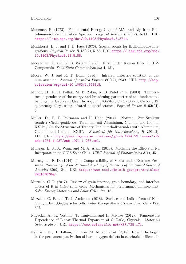
Bibliography 107
Monemar, B. (1973). Fundamental Energy Gaps of AlAs and Alp from Pho-toluminescence Excitation Spectra. Physical Review B 8(12), 5711. URLhttps://link.aps.org/doi/10.1103/PhysRevB.8.5711.
Monkhorst, H. J. and J. D. Pack (1976). Special points for Brillouin-zone inte-grations. Physical Review B 13(12), 5188. URL https://link.aps.org/doi/10.1103/PhysRevB.13.5188.
Mooradian, A. and G. B. Wright (1966). First Order Raman Effec in III-VCompounds. Solid State Communications 4, 431.
Moore, W. J. and R. T. Holm (1996). Infrared dielectric constant of gal-lium arsenide. Journal of Applied Physics 80(12), 6939. URL http://aip.scitation.org/doi/10.1063/1.363818.
Muñoz, M., F. H. Pollak, M. B. Zakia, N. B. Patel et al. (2000). Tempera-ture dependence of the energy and broadening parameter of the fundamentalband gap of GaSb and Ga1−xInxAsySb1−y/GaSb (0.07<x<0.22, 0.05<y<0.19)quaternary alloys using infrared photoreflectance. Physical Review B 62(24),5.
Müller, D., F. E. Poltmann and H. Hahn (2014). Notizen: Zur Strukturternärer Chalkogenide des Thalliums mit Aluminium, Gallium und Indium,XXII* / On the Structure of Ternary Thalliumchalkogenides with Aluminium,Gallium and Indium, XXII*. Zeitschrift für Naturforschung B 29(1-2),117. URL https://www.degruyter.com/view/j/znb.1974.29.issue-1-2/znb-1974-1-237/znb-1974-1-237.xml.
Mungan, E. S., X. Wang and M. A. Alam (2013). Modeling the Effects of NaIncorporation on CIGS Solar Cells. IEEE Journal of Photovoltaics 3(1), 451.
Murnaghan, F. D. (1944). The Compressibility of Media under Extreme Pres-sures. Proceedings of the National Academy of Sciences of the United States ofAmerica 30(9), 244. URL https://www.ncbi.nlm.nih.gov/pmc/articles/PMC1078704/.
Muzzillo, C. P. (2017). Review of grain interior, grain boundary, and interfaceeffects of K in CIGS solar cells: Mechanisms for performance enhancement.Solar Energy Materials and Solar Cells 172, 18.
Muzzillo, C. P. and T. J. Anderson (2018). Surface and bulk effects of K inCu1−xKxIn1−yGaySe2 solar cells. Solar Energy Materials and Solar Cells 179,362.
Nagaoka, A., K. Yoshino, T. Taniyama and H. Miyake (2012). TemperatureDependence of Linear Thermal Expansion of CuGaSe2 Crystals. MaterialsScience Forum URL https://www.scientific.net/MSF.725.171.
Nampalli, N., B. Hallam, C. Chan, M. Abbott et al. (2015). Role of hydrogenin the permanent passivation of boron-oxygen defects in czochralski silicon. In

108 Bibliography
2015 IEEE 42nd Photovoltaic Specialist Conference (PVSC), 1–3. IEEE, NewOrleans, LA. URL http://ieeexplore.ieee.org/document/7356404/.
Neumann, H. (1986). Lattice vibrational, thermal and mechanical properties ofCuInSe2. Solar Cells 16, 399.
Nichols, D. N., D. S. Rimai and R. J. Sladek (1980). Elastic anharmonicity of InP:Its relationship to the high pressure transition. Solid State Communications36(8), 667. URL http://www.sciencedirect.com/science/article/pii/0038109880902057.
Niles, D., K. Ramanathan, F. Hasoon, R. Noufi et al. (1997). Na impurity chem-istry in photovoltaic. Journal of Vacuum Science & Technology A 15(6), 3044.
Novikova, S. (1966). Chapter 2 Thermal Expansion. In Semiconductors andSemimetals , volume 2, 33–48. Elsevier. URL https://linkinghub.elsevier.com/retrieve/pii/S008087840860160X.
Oikkonen, L. E., M. G. Ganchenkova, A. P. Seitsonen and R. M. Nieminen (2013).Effect of sodium incorporation into CuInSe2 from first principles. Journal ofApplied Physics 114(8), 083503.
Olego, D. and M. Cardona (1982). Pressure dependence of Raman phonons of Geand 3C–SiC. Physical Review B 25(2), 1151. URL https://link.aps.org/doi/10.1103/PhysRevB.25.1151.
Ortega, J. E. and F. J. Himpsel (1993). Inverse-photoemission study of Ge(100),Si(100), and GaAs(100): Bulk bands and surface states. Physical Review B47(4), 2130. URL https://link.aps.org/doi/10.1103/PhysRevB.47.2130.
Osterwald, C., A. Anderberg, S. Rummel and L. Ottoson (2002). Degradationanalysis of weathered crystalline-silicon PV modules. In Conference Record ofthe Twenty-Ninth IEEE Photovoltaic Specialists Conference, 2002., 1392–1395.ISSN: 1060-8371.
Paier, J., R. Hirschl, M. Marsman and G. Kresse (2005). The Perdew–Burke–Ernzerhof exchange-correlation functional applied to the G2-1 test set using aplane-wave basis set. The Journal of Chemical Physics 122(23), 234102. URLhttp://aip.scitation.org/doi/10.1063/1.1926272.
Paier, J., M. Marsman, K. Hummer, G. Kresse et al. (2006). Screened hybriddensity functionals applied to solids. The Journal of Chemical Physics 124(15),154709. URL http://aip.scitation.org/doi/10.1063/1.2187006.
Palmer, D. (2019). Properties of III-V Semiconductors. URL http://www.semiconductors.co.uk/propiiiv5653.htm.
Parker, J. H., D. W. Feldman and M. Ashkin (1967). Raman scattering by siliconand germanium. Physical Review 155(3), 712. URL http://link.aps.org/doi/10.1103/PhysRev.155.712.
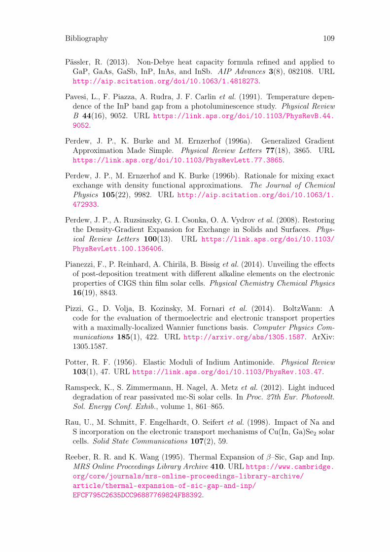
Bibliography 109
Pässler, R. (2013). Non-Debye heat capacity formula refined and applied toGaP, GaAs, GaSb, InP, InAs, and InSb. AIP Advances 3(8), 082108. URLhttp://aip.scitation.org/doi/10.1063/1.4818273.
Pavesi, L., F. Piazza, A. Rudra, J. F. Carlin et al. (1991). Temperature depen-dence of the InP band gap from a photoluminescence study. Physical ReviewB 44(16), 9052. URL https://link.aps.org/doi/10.1103/PhysRevB.44.9052.
Perdew, J. P., K. Burke and M. Ernzerhof (1996a). Generalized GradientApproximation Made Simple. Physical Review Letters 77(18), 3865. URLhttps://link.aps.org/doi/10.1103/PhysRevLett.77.3865.
Perdew, J. P., M. Ernzerhof and K. Burke (1996b). Rationale for mixing exactexchange with density functional approximations. The Journal of ChemicalPhysics 105(22), 9982. URL http://aip.scitation.org/doi/10.1063/1.472933.
Perdew, J. P., A. Ruzsinszky, G. I. Csonka, O. A. Vydrov et al. (2008). Restoringthe Density-Gradient Expansion for Exchange in Solids and Surfaces. Phys-ical Review Letters 100(13). URL https://link.aps.org/doi/10.1103/PhysRevLett.100.136406.
Pianezzi, F., P. Reinhard, A. Chirilă, B. Bissig et al. (2014). Unveiling the effectsof post-deposition treatment with different alkaline elements on the electronicproperties of CIGS thin film solar cells. Physical Chemistry Chemical Physics16(19), 8843.
Pizzi, G., D. Volja, B. Kozinsky, M. Fornari et al. (2014). BoltzWann: Acode for the evaluation of thermoelectric and electronic transport propertieswith a maximally-localized Wannier functions basis. Computer Physics Com-munications 185(1), 422. URL http://arxiv.org/abs/1305.1587. ArXiv:1305.1587.
Potter, R. F. (1956). Elastic Moduli of Indium Antimonide. Physical Review103(1), 47. URL https://link.aps.org/doi/10.1103/PhysRev.103.47.
Ramspeck, K., S. Zimmermann, H. Nagel, A. Metz et al. (2012). Light induceddegradation of rear passivated mc-Si solar cells. In Proc. 27th Eur. Photovolt.Sol. Energy Conf. Exhib., volume 1, 861–865.
Rau, U., M. Schmitt, F. Engelhardt, O. Seifert et al. (1998). Impact of Na andS incorporation on the electronic transport mechanisms of Cu(In, Ga)Se2 solarcells. Solid State Communications 107(2), 59.
Reeber, R. R. and K. Wang (1995). Thermal Expansion of β–Sic, Gap and Inp.MRS Online Proceedings Library Archive 410. URL https://www.cambridge.org/core/journals/mrs-online-proceedings-library-archive/article/thermal-expansion-of-sic-gap-and-inp/EFCF795C2635DCC96887769824FB8392.
110 Bibliography
Reining, L. (2018). The GW approximation: content, successes and limitations.Wiley Interdisciplinary Reviews: Computational Molecular Science 8(3), e1344.URL http://onlinelibrary.wiley.com/doi/abs/10.1002/wcms.1344.
Rincón, C. and F. J. Ramírez (1992). Lattice vibrations of CuInSe2 and CuGaSe2by Raman microspectrometry. Journal of Applied Physics 72(9), 4321. URLhttp://aip.scitation.org/doi/10.1063/1.352195.
Roa, L., C. Rincón, J. González and M. Quintero (1990). Analysis of direct exci-ton transitions in CuGa(SxSe1−x)2 alloys. Journal of Physics and Chemistry ofSolids 51(6), 551. URL http://www.sciencedirect.com/science/article/pii/0022369790901629.
Rode, D. L. (1970). Electron Mobility in Direct-Gap Polar Semiconductors.Physical Review B 2(4), 1012. URL https://link.aps.org/doi/10.1103/PhysRevB.2.1012.
Rohlfing, M., P. Krüger and J. Pollmann (1993). Quasiparticle band-structure cal-culations for C, Si, Ge, GaAs, and SiC using Gaussian-orbital basis sets. Phys-ical Review B 48(24), 17791. URL https://link.aps.org/doi/10.1103/PhysRevB.48.17791.
Rong-Tie, H., Z. Ming, S. Li-Fang, C. Chuan-Bing et al. (2017). Synthesis andPhysical Properties of Solar Material CuxLi1−xInSe2. Journal of InorganicMaterials 32(1), 101.
Ruckh, M., D. Schmid, M. Kaiser, R. Schaffler et al. (1996). Influence of substrateson the electrical properties of Cu(In,Ga)Se2 thin films. Solar Energy Materialsand Solar Cells 41-42, 335.
Rudmann, D., A. F. da Cunha, M. Kaelin, F. Kurdesau et al. (2004). Efficiencyenhancement of Cu(In,Ga)Se2 solar cells due to post-deposition Na incorpora-tion. Applied Physics Letters 84(7), 1129.
Saarinen, K., T. Laine, S. Kuisma, J. Nissilä et al. (1997). Observationof native Ga vacancies in GaN by positron annihilation. MRS OnlineProceedings Library Archive 482. URL https://www.cambridge.org/core/journals/mrs-online-proceedings-library-archive/article/observation-of-native-ga-vacancies-in-gan-by-positron-annihilation/BD4C0A534F4DE0BF4BA220C3F907BF8C.
Salomé, P., H. Rodriguez-Alvarez and S. Sadewasser (2015). Incorporation ofalkali metals in chalcogenide solar cells. Solar Energy Materials and SolarCells 143, 9.
Sansone, G., A. Ferretti and L. Maschio (2017). Ab initio electronic transportand thermoelectric properties of solids from full and range-separated hybridfunctionals. The Journal of Chemical Physics 147(11), 114101. URL http://aip.scitation.org/doi/10.1063/1.4986398.

Bibliography 111
Scheidemantel, T. J., C. Ambrosch-Draxl, T. Thonhauser, J. V. Badding et al.(2003). Transport coefficients from first-principles calculations. Physical ReviewB 68(12). URL https://link.aps.org/doi/10.1103/PhysRevB.68.125210.
Schimka, L., J. Harl and G. Kresse (2011). Improved hybrid functional for solids:The HSEsol functional. The Journal of Chemical Physics 134(2), 024116. URLhttp://aip.scitation.org/doi/10.1063/1.3524336.
Schmidt, J., A. Aberle and R. Hezel (1997). Investigation of carrier lifetimeinstabilities in Cz-grown silicon. In Conference Record of the Twenty SixthIEEE Photovoltaic Specialists Conference - 1997 , 13–18. ISSN: 0160-8371.
Schöppe, P., S. Schönherr, R. Wuerz, W. Wisniewski et al. (2017). Rubidium seg-regation at random grain boundaries in Cu(In,Ga)Se2 absorbers. Nano Energy42, 307.
Schubert, H. and R. Hoppe (1970). Zur Kenntnis der RbInS2-Strukturfamilie. Z.Naturforsch 25b, 886.
Seeger, A. (1974). The study of defects in crystals by positron annihilation.Applied physics 4(3), 183. URL https://doi.org/10.1007/BF00884229.
Sekine, T., K. Uchinokura and E. Matsuura (1976). Two-phonon Raman scatter-ing in GaSb. Solid State Communications 18(9-10), 1337.
Shimazaki, T. and Y. Asai (2008). Band structure calculations based on screenedFock exchange method. Chemical Physics Letters 466(1-3), 91. URL https://linkinghub.elsevier.com/retrieve/pii/S0009261408013717.
Shimazaki, T. and Y. Asai (2009). First principles band structure calculationsbased on self-consistent screened Hartree–Fock exchange potential. The Journalof Chemical Physics 130(16), 164702. URL https://aip-scitation-org.bases-doc.univ-lorraine.fr/doi/10.1063/1.3119259.
Shimazaki, T. and T. Nakajima (2014). Dielectric-dependent screened Hartree–Fock exchange potential and Slater-formula with Coulomb-hole interaction forenergy band structure calculations. The Journal of Chemical Physics 141(11),114109. URL http://aip.scitation.org/doi/10.1063/1.4895623. Cita-tion Key Alias: shimazaki.nakajima_2014_Dielectricdependenta.
Shin, D., J. Kim, T. Gershon, R. Mankad et al. (2016). Effects of the incorporationof alkali elements on Cu(In,Ga)Se2 thin film solar cells. Solar Energy Materialsand Solar Cells 157, 695.
Singh, J. (1992). Physics of Semiconductors and Their Heterostructures , vol-ume 84. McGraw-Hill New York.
Skone, J. H., M. Govoni and G. Galli (2014). Self-consistent hybrid functionalfor condensed systems. Physical Review B 89(19). URL https://link.aps.org/doi/10.1103/PhysRevB.89.195112.

112 Bibliography
Slater, J. C. (1929). The Theory of Complex Spectra. Physical Review 34(10),1293. URL https://link.aps.org/doi/10.1103/PhysRev.34.1293.
Slutsky, L. J. and C. W. Garland (1959). Elastic Constants of Indium Antimonidefrom 4.2K to 300K. Physical Review 113(1), 167. URL https://link.aps.org/doi/10.1103/PhysRev.113.167.
Solar Frontier (2019). Solar frontier achieves world record thin-film solar cell ef-ficiency of 23.35%. URL http://www.solar-frontier.com/eng/news/2019/0117_press.html. [Online; accessed 5-March-2019].
Soma, T., J. Satoh and H. Matsuo (1982). Thermal expansion coefficient ofGaAs and InP. Solid State Communications 42(12), 889. URL https://linkinghub.elsevier.com/retrieve/pii/0038109882902332.
Sommer, H. and R. Hoppe (1977). Die Kristallstruktur von Cs2S, mit einerBemerkung über Cs2Se, Cs2Te, Rb2Se und Rb2Te. Zeitschrift für anorganischeund allgemeine Chemie 429(1), 118. URL http://doi.wiley.com/10.1002/zaac.19774290116.
Sopori, B. (1999). Impurities and defects in photovoltaic si devices: A re-view. Technical Report NREL/CP-520-27524, National Renewable EnergyLab., Golden, CO (US). URL https://www.osti.gov/biblio/753811.
Sparks, P. W. and C. A. Swenson (1967). Thermal Expansions from 2 to 40 Kof Ge, Si, and Four III-V Compounds. Physical Review 163(3), 779. URLhttps://link.aps.org/doi/10.1103/PhysRev.163.779.
Spiess, H. W., U. Haeberlen, G. Brandt, A. Räuber et al. (1974). NuclearMagnetic Resonance in IB–III–VI2 Semiconductors. physica status solidi(b) 62(1), 183. URL http://onlinelibrary.wiley.com/doi/abs/10.1002/pssb.2220620118.
Staroverov, V. N., G. E. Scuseria, J. Tao and J. P. Perdew (2004). Tests of aladder of density functionals for bulk solids and surfaces. Physical Review B69(7). URL https://link.aps.org/doi/10.1103/PhysRevB.69.075102.
Straumanis, M. E. and C. D. Kim (1965). Lattice Parameters, Thermal ExpansionCoefficients, Phase Width, and Perfection of the Structure of GaSb and InSb.Journal of Applied Physics 36(12), 3822. URL http://aip.scitation.org/doi/10.1063/1.1713955.
Sturge, M. D. (1962). Optical absorption of gallium arsenide between 0.6 and2.75 eV. Physical Review 127(3), 768.
Sun, Y., S. Lin, W. Li, S. Cheng et al. (2017). Review on Alkali Element Dopingin Cu(In,Ga)Se2 Thin Films and Solar Cells. Engineering 3(4), 452.
Taguchi, N., S. Tanaka and S. Ishizuka (2018). Direct insights into RbInSe2 for-mation at Cu(In,Ga)Se2 thin film surface with RbF postdeposition treatment.Applied Physics Letters 113(11), 113903.
Bibliography 113
Tiginyanu, I. M. (1999). Raman Modes in Porous GaP under Hydrostatic Pres-sure. Physica Status Solidi (b) 211, 6.
Tinoco, T., J. P. Itié, A. Polian, A. San Miguel et al. (1994). Combined x-rayabsorption and x-ray diffraction studies of CuGaS2, CuGaSe2, CuFeS2 andCuFeSe2 under high pressure. Le Journal de Physique IV 04(C9), C9. URLhttp://www.edpsciences.org/10.1051/jp4:1994923.
Tinoco, T., A. Polian, D. Gómez and J. P. Itié (1996). Structural Stud-ies of CuInS2 and CuInSe2 under High Pressure. physica status solidi (b)198(1), 433. URL http://onlinelibrary.wiley.com/doi/abs/10.1002/pssb.2221980156.
Tinoco, T., M. Quintero and C. Rincón (1991). Variation of the energy gap withcomposition in AIBIIICV I
2 chalcopyrite-structure alloys. Physical Review B44(4), 1613. URL https://link.aps.org/doi/10.1103/PhysRevB.44.1613.
Urbaniak, A., M. Igalson, F. Pianezzi, S. Bücheler et al. (2014). Effects of Naincorporation on electrical properties of Cu(In,Ga)Se2-based photovoltaic de-vices on polyimide substrates. Solar Energy Materials and Solar Cells 128,52.
Van de Walle, C. G. (1994). Energies of various configurations of hydrogen insilicon. Physical Review B 49(7), 4579. URL https://link.aps.org/doi/10.1103/PhysRevB.49.4579.
Van de Walle, C. G., P. J. H. Denteneer, Y. Bar-Yam and S. T. Pantelides (1989).Theory of hydrogen diffusion and reactions in crystalline silicon. Physical Re-view B 39(15), 10791. URL https://link.aps.org/doi/10.1103/PhysRevB.39.10791.
Van de Walle, C. G. and J. Neugebauer (2006). Hydrogen in semiconductors.Annual Review of Materials Research 36(1), 179. URL https://doi.org/10.1146/annurev.matsci.36.010705.155428.
Varshni, Y. P. (1967). Temperature dependence of the energy gap in semiconduc-tors. Physica 34(1), 149. URL http://www.sciencedirect.com/science/article/pii/0031891467900626.
Vilalta-Clemente, A., M. Raghuwanshi, S. Duguay, C. Castro et al. (2018). Ru-bidium distribution at atomic scale in high efficient Cu(In,Ga)Se2 thin-filmsolar cells. Applied Physics Letters 112(10), 103105.
Vosko, S. H., L. Wilk and M. Nusair (1980). Accurate spin-dependent elec-tron liquid correlation energies for local spin density calculations: a criti-cal analysis. Canadian Journal of Physics 58(8), 1200. URL http://www.nrcresearchpress.com/doi/10.1139/p80-159.
Vurgaftman, I., J. R. Meyer and L. R. Ram-Mohan (2001). Band parameters forIII-V compound semiconductors and their alloys. Journal of Applied Physics89(11 I), 5815.
114 Bibliography
Ward, M. D., E. A. Pozzi, R. P. Van Duyne and J. A. Ibers (2014). Syn-theses, structures, and optical properties of the indium/germanium se-lenides Cs4in8gese16, CsInSe2, and CsInGeSe4. Journal of Solid State Chem-istry 212, 191. URL https://linkinghub.elsevier.com/retrieve/pii/S0022459614000279.
Weber, J. and M. I. Alonso (1989). Near-band-gap photoluminescence of Si-Gealloys. Physical Review B 40(8), 5683. URL https://link.aps.org/doi/10.1103/PhysRevB.40.5683.
Wei, S. and A. Zunger (1995). Band offsets and optical bowings of chalcopyritesand Zn–based II–VI alloys. Journal of Applied Physics 78(6), 3846. URLhttp://aip.scitation.org/doi/10.1063/1.359901.
Wei, S.-H., S. B. Zhang and A. Zunger (1999). Effects of Na on the electrical andstructural properties of CuInSe2. Journal of Applied Physics 85(10), 7214.
Weil, R. and W. O. Groves (1968). The Elastic Constants of Gallium Phosphide.Journal of Applied Physics 39(9).
Weiss, T. P., S. Nishiwaki, B. Bissig, R. Carron et al. (2018). Injection CurrentBarrier Formation for RbF Postdeposition-Treated Cu(In,Ga)Se2 -Based SolarCells. Advanced Materials Interfaces 5(4), 1701007.
Wenham, A. C. n., S. Wenham, R. Chen, C. Chan et al. (2018). Hydrogen-Induced Degradation. In 2018 IEEE 7th World Conference on PhotovoltaicEnergy Conversion (WCPEC) (A Joint Conference of 45th IEEE PVSC, 28thPVSEC & 34th EU PVSEC), 0001–0008. IEEE, Waikoloa Village, HI. URLhttps://ieeexplore.ieee.org/document/8548100/.
Werner, A., H. D. Hochheimer and A. Jayaraman (1981). Pressure-inducedphase transformations in the chalcopyrite-structure compounds: CuGaS2 andAgGaS2. Physical Review B 23(8), 3836. URL https://link.aps.org/doi/10.1103/PhysRevB.23.3836.
Werner, F., M. H. Wolter, S. Siebentritt, G. Sozzi et al. (2018). Alkali treatmentsof Cu(In,Ga)Se2 thin-film absorbers and their impact on transport barriers.Progress in Photovoltaics: Research and Applications 26(11), 911.
Wilking, S., A. Herguth and G. Hahn (2013). Influence of hydrogen on theregeneration of boron-oxygen related defects in crystalline silicon. Journal ofApplied Physics 113(19), 194503. URL http://aip.scitation.org/doi/10.1063/1.4804310.
Wu, M. and C. Chen (1992). Photoluminescence of high–quality GaSb grown fromGa– and Sb–rich solutions by liquid–phase epitaxy. Journal of Applied Physics72(9), 4275. URL http://aip.scitation.org/doi/10.1063/1.352216.
Wuerz, R., A. Eicke, F. Kessler, S. Paetel et al. (2012). CIGS thin-film solar cellsand modules on enamelled steel substrates. Solar Energy Materials and SolarCells 100, 132.

Bibliography 115
Wuerz, R., W. Hempel and P. Jackson (2018). Diffusion of Rb in polycrystallineCu(In,Ga)Se2 layers and effect of Rb on solar cell parameters of Cu(In,Ga)Se2thin-film solar cells. Journal of Applied Physics 124(16), 165305.
Xu, C., C. Wang, C. Chan and K. Ho (1991). Theory of the thermal expansionof Si and diamond. Phys. Rev. B 43(6).
Yu, P. and M. Cardona (2010). Fundamentals of Semiconductors: Physicsand Materials Properties . Graduate Texts in Physics. Springer-Verlag,Berlin Heidelberg, 4 edition. URL https://www.springer.com/gp/book/9783642007095.
Yuan, Z.-K., S. Chen, Y. Xie, J.-S. Park et al. (2016). Na-Diffusion Enhancedp-type Conductivity in Cu(In,Ga)Se2 : A New Mechanism for Efficient Dopingin Semiconductors. Advanced Energy Materials 6(24), 1601191.
Zeng, H.-Y., F.-K. Zheng, R.-P. Chen, Z.-C. Dong et al. (2007). Reactive fluxsyntheses, crystal structures and band gaps of AInS2 (A=Rb, Cs). Journalof Alloys and Compounds 432(1-2), 69. URL http://linkinghub.elsevier.com/retrieve/pii/S0925838806007109.
Zhao, Y. and D. G. Truhlar (2006). A new local density functional for main-groupthermochemistry, transition metal bonding, thermochemical kinetics, and non-covalent interactions. The Journal of Chemical Physics 125(19), 194101. URLhttp://aip.scitation.org/doi/10.1063/1.2370993.
Zhao, Y. and D. G. Truhlar (2008). The M06 suite of density functionals for maingroup thermochemistry, thermochemical kinetics, noncovalent interactions, ex-cited states, and transition elements: two new functionals and systematic test-ing of four M06-class functionals and 12 other functionals. Theoretical Chem-istry Accounts 120(1-3), 215. URL http://link.springer.com/10.1007/s00214-007-0310-x.
Zintl, E., A. Harder and B. Dauth (1934). Gitterstruktur der Oxyde, Sulfide,Selenide und Telluride des Lithiums, Natriums und Kaliums. Zeitschrift fürElektrochemie und angewandte physikalische Chemie 40(8), 588. URL https://onlinelibrary.wiley.com/doi/abs/10.1002/bbpc.19340400811.
Zollner, S., S. Gopalan and M. Cardona (1991). The temperature dependenceof the band gaps in InP, InAs, InSb, and GaSb. Solid State Communica-tions 77(7), 485. URL https://linkinghub.elsevier.com/retrieve/pii/003810989190725B.

List of Contributions and Awards
Awards
Best poster presented in symposium A"First-Principles Investigation of Chemical Composition Effects on Thermody-namic and Optoelectronic Properties of Chalcopyrites"F. Lafond, Ph. Baranek, A. PostnikovE-MRS 2018 Spring Meeting, Strasbourg, France
Paper
"Effects of the Copper Substitution by Alkali Metals on the Properties of Chal-copyrites for Tandem Applications: Insights from Theory."F. Lafond, Ph. Baranek, A. PostnikovSubmitted to Inorganic Chemistry
Contributions to conferences
Talk"First-Principles Approach of the Structural, Electronic, Dynamical and Ther-modynamic Properties of Defective Silicon: Influence of the Temperature on theFormation Energy of Defect."F. Lafond, Ph. Baranek, A. PostnikovE-MRS 2017 Fall Meeting, Warsaw, Poland
Talk"First-Principles Investigation of Chemical Composition Effects on Thermody-namic and Optoelectronic Properties of Chalcopyrites"F. Lafond, Ph. Baranek, A. PostnikovInternational Conference on Ternary and Multinary Compounds (ICTMC-21),Boulder, Colorado, USA
Poster"First-Principles Approach of the Structural, Electronic and Dynamical Proper-ties of SixGe1−x (0 ≤ x ≤ 1), SiC, GaX (with X = P, As, Sb): A Study of theHybrid Functionals Performance."
118 List of Contributions and Awards
F. Lafond, Ph. Baranek, A. PostnikovXXIX IUPAP Conference in Computational Physics (CCP2017), Paris, France
Poster"Hybrid Functionals Approach of the Structural, Electronic and Dynamical Prop-erties of Semiconductors for Photovoltaic Applications."F. Lafond, B. Civalleri, Ph. Baranek, A. Postnikov11th Triennial Congress of the World Association of Theoretical and Computa-tional Chemists (WATOC), Munich, Germany
Poster"First-Principles Investigation of Chemical Composition Effects on Thermody-namic and Optoelectronic Properties of Chalcopyrites"F. Lafond, Ph. Baranek, A. PostnikovE-MRS 2018 Spring Meeting, Strasbourg, France
Summary
The electrical properties of semiconductors, such as concentrations and mobili-ties of charge careers, are strongly influenced by the types of dopants and defectsinserted or formed during the synthesis of materials. In the field of photovoltaics,these defects lead to various perturbations (distortions of the phase stability, ap-pearance of supplementary energy levels in the band gap, etc.) and can degradethe efficiency and durability of solar cells. In this context, ab initio simulationmethods, such as Hartree-Fock (HF) or those implemented in the framework ofdensity functional theory (DFT), are relevant to understand these behavioursand thus improve and optimise the photovoltaic materials. However, a qualita-tive and quantitative description of properties, such as the electronic structures,requires sophisticated but time consuming techniques, implementing, e.g., theGW approximation. An interesting alternative to this can be provided by hybridfunctionals, which combine a certain percentage of the HF exact exchange withthe exchange-correlation provided by functionals from the various realisations ofthe DFT.Firstly, hybrid functionals were optimised in order to accurately describe the bandgap for different compounds by carefully adjusting the percentage of the HF ex-act exchange in the exchange part of the PBE and PBEsol functionals, suggestedwithin the generalised gradient approximation of the DFT. The materials investi-gated were Si, Ge, SiGe, III-V and the chalcopyrite-type compounds. The resultsobtained by this approach were compared to those available from the literature,paying particular attention to the GW calculation results. The description ofthe electronic properties, such as the band structures, with the hybrid functionalturns out to generally match that from the GW calculations. Structural anddielectric properties were also in good agreement with the experimental data.The temperature evolution of various thermodynamic properties, like the heatcapacity, was calculated via the quasi-harmonic approximation (QHA). In thislatter approximation and for the range of studied materials, optimised hybridfunctionals however do not bring any noticeable improvement against the ex-isting functionals. Nevertheless, they bring about a coherent description of thematerials.Secondly, these optimised hybrid functionals were used to systematically describethe impact of chemical composition on chalcopyrite’s properties for tandem solarcells. First, they enable the determination of the compositions, structural andelectrical properties of CuGaxIn1−x(SySe1−y)2 for band gap specific to this kind ofapplication. Then, the effect of alkali metals incorporations into the chalcopyrite-type bulk materials was addressed. Doping with alkali metals leads to a major

120 Summary
enhancement of the photovoltaic efficiency of the chalcopyrite-type compounds.Interesting results have been obtained concerning the substitution of copper byLi, Na, K, Rb and Cs. The impact of these dopants on the band gap was in-terpreted via the structural evolution and the thermodynamic stability of thedifferent crystallines phases that can exist within the material.Finally, hydrogen, iron and boron point defects in silicon were simulated as a partof a preliminary study on the light and elevated temperature induced degradation(LeTID) which is among the major challenges in the study of the ageing processof the silicon solar cells.
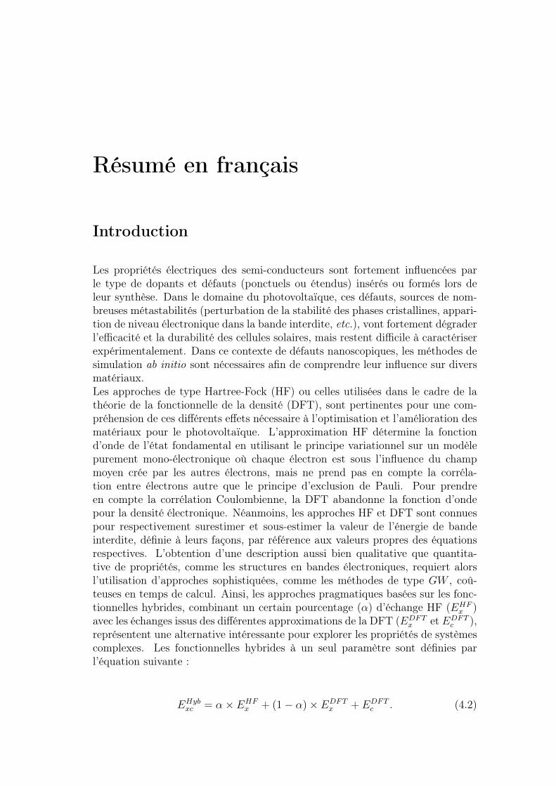
Résumé en français
Introduction
Les propriétés électriques des semi-conducteurs sont fortement influencées parle type de dopants et défauts (ponctuels ou étendus) insérés ou formés lors deleur synthèse. Dans le domaine du photovoltaïque, ces défauts, sources de nom-breuses métastabilités (perturbation de la stabilité des phases cristallines, appari-tion de niveau électronique dans la bande interdite, etc.), vont fortement dégraderl’efficacité et la durabilité des cellules solaires, mais restent difficile à caractériserexpérimentalement. Dans ce contexte de défauts nanoscopiques, les méthodes desimulation ab initio sont nécessaires afin de comprendre leur influence sur diversmatériaux.Les approches de type Hartree-Fock (HF) ou celles utilisées dans le cadre de lathéorie de la fonctionnelle de la densité (DFT), sont pertinentes pour une com-préhension de ces différents effets nécessaire à l’optimisation et l’amélioration desmatériaux pour le photovoltaïque. L’approximation HF détermine la fonctiond’onde de l’état fondamental en utilisant le principe variationnel sur un modèlepurement mono-électronique où chaque électron est sous l’influence du champmoyen crée par les autres électrons, mais ne prend pas en compte la corréla-tion entre électrons autre que le principe d’exclusion de Pauli. Pour prendreen compte la corrélation Coulombienne, la DFT abandonne la fonction d’ondepour la densité électronique. Néanmoins, les approches HF et DFT sont connuespour respectivement surestimer et sous-estimer la valeur de l’énergie de bandeinterdite, définie à leurs façons, par référence aux valeurs propres des équationsrespectives. L’obtention d’une description aussi bien qualitative que quantita-tive de propriétés, comme les structures en bandes électroniques, requiert alorsl’utilisation d’approches sophistiquées, comme les méthodes de type GW , coû-teuses en temps de calcul. Ainsi, les approches pragmatiques basées sur les fonc-tionnelles hybrides, combinant un certain pourcentage (α) d’échange HF (EHF
x )avec les échanges issus des différentes approximations de la DFT (EDFT
x et EDFTc ),
représentent une alternative intéressante pour explorer les propriétés de systèmescomplexes. Les fonctionnelles hybrides à un seul paramètre sont définies parl’équation suivante :
EHybxc = α× EHF
x + (1− α)× EDFTx + EDFT
c . (4.2)
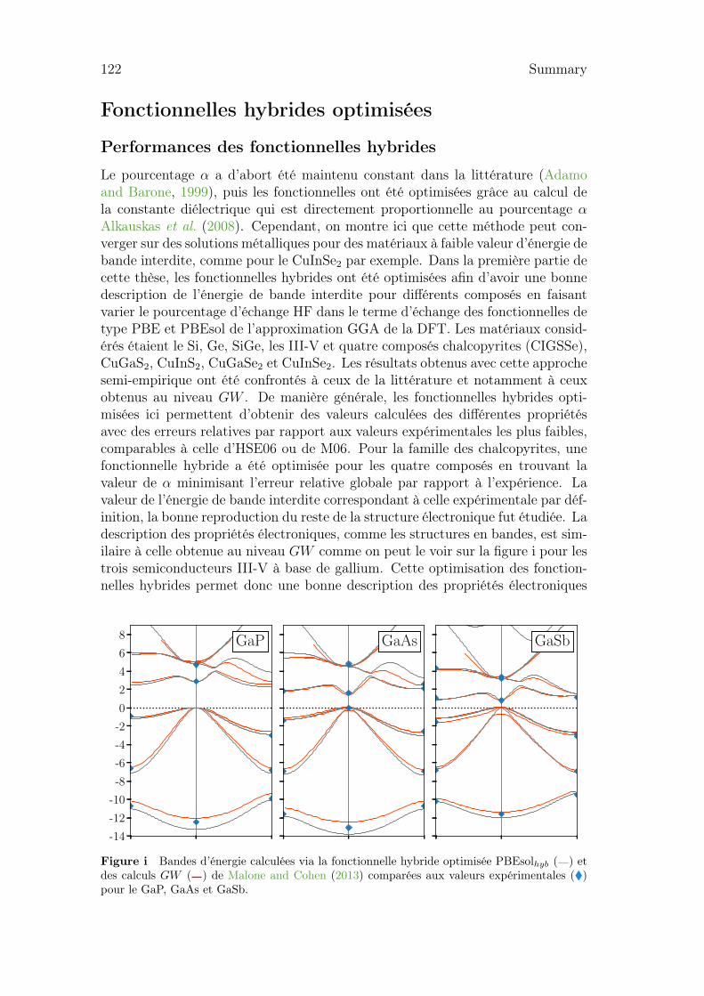
122 Summary
Fonctionnelles hybrides optimisées
Performances des fonctionnelles hybrides
Le pourcentage α a d’abort été maintenu constant dans la littérature (Adamoand Barone, 1999), puis les fonctionnelles ont été optimisées grâce au calcul dela constante diélectrique qui est directement proportionnelle au pourcentage αAlkauskas et al. (2008). Cependant, on montre ici que cette méthode peut con-verger sur des solutions métalliques pour des matériaux à faible valeur d’énergie debande interdite, comme pour le CuInSe2 par exemple. Dans la première partie decette thèse, les fonctionnelles hybrides ont été optimisées afin d’avoir une bonnedescription de l’énergie de bande interdite pour différents composés en faisantvarier le pourcentage d’échange HF dans le terme d’échange des fonctionnelles detype PBE et PBEsol de l’approximation GGA de la DFT. Les matériaux consid-érés étaient le Si, Ge, SiGe, les III-V et quatre composés chalcopyrites (CIGSSe),CuGaS2, CuInS2, CuGaSe2 et CuInSe2. Les résultats obtenus avec cette approchesemi-empirique ont été confrontés à ceux de la littérature et notamment à ceuxobtenus au niveau GW . De manière générale, les fonctionnelles hybrides opti-misées ici permettent d’obtenir des valeurs calculées des différentes propriétésavec des erreurs relatives par rapport aux valeurs expérimentales les plus faibles,comparables à celle d’HSE06 ou de M06. Pour la famille des chalcopyrites, unefonctionnelle hybride a été optimisée pour les quatre composés en trouvant lavaleur de α minimisant l’erreur relative globale par rapport à l’expérience. Lavaleur de l’énergie de bande interdite correspondant à celle expérimentale par déf-inition, la bonne reproduction du reste de la structure électronique fut étudiée. Ladescription des propriétés électroniques, comme les structures en bandes, est sim-ilaire à celle obtenue au niveau GW comme on peut le voir sur la figure i pour lestrois semiconducteurs III-V à base de gallium. Cette optimisation des fonction-nelles hybrides permet donc une bonne description des propriétés électroniques
-14
-12
-10
-8
-6
-4
-2
0
2
4
6
8 GaP GaAs GaSb
-14
-12
-10
-8
-6
-4
-2
0
2
4
6
8 AlP
En
ergy
/eV
AlAs AlSb
L Γ X-14
-12
-10
-8
-6
-4
-2
0
2
4
6
8 InP
L Γ X
InAs
L Γ X
InSb
Figure i Bandes d’énergie calculées via la fonctionnelle hybride optimisée PBEsolhyb ( ) etdes calculs GW ( ) de Malone and Cohen (2013) comparées aux valeurs expérimentales ()pour le GaP, GaAs et GaSb.
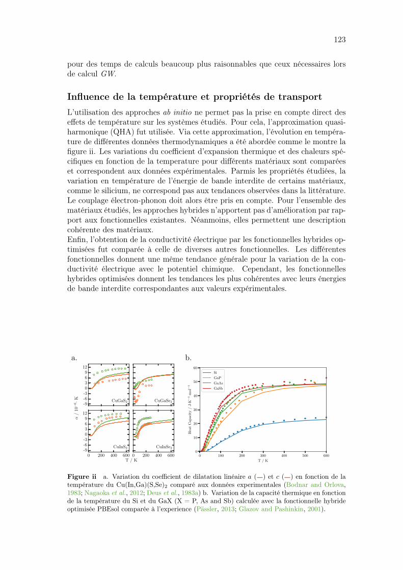
123
pour des temps de calculs beaucoup plus raisonnables que ceux nécessaires lorsde calcul GW.
Influence de la température et propriétés de transport
L’utilisation des approches ab initio ne permet pas la prise en compte direct deseffets de température sur les systèmes étudiés. Pour cela, l’approximation quasi-harmonique (QHA) fut utilisée. Via cette approximation, l’évolution en tempéra-ture de différentes données thermodynamiques a été abordée comme le montre lafigure ii. Les variations du coefficient d’expansion thermique et des chaleurs spé-cifiques en fonction de la temperature pour différents matériaux sont comparéeset correspondent aux données expérimentales. Parmis les propriétés étudiées, lavariation en température de l’énergie de bande interdite de certains matériaux,comme le silicium, ne correspond pas aux tendances observées dans la littérature.Le couplage électron-phonon doit alors être pris en compte. Pour l’ensemble desmatériaux étudiés, les approches hybrides n’apportent pas d’amélioration par rap-port aux fonctionnelles existantes. Néanmoins, elles permettent une descriptioncohérente des matériaux.Enfin, l’obtention de la conductivité électrique par les fonctionnelles hybrides op-timisées fut comparée à celle de diverses autres fonctionnelles. Les différentesfonctionnelles donnent une même tendance générale pour la variation de la con-ductivité électrique avec le potentiel chimique. Cependant, les fonctionnelleshybrides optimisées donnent les tendances les plus cohérentes avec leurs énergiesde bande interdite correspondantes aux valeurs expérimentales.
a. b.
-9-6-30369
12
α/
10−
6·K CuGaS2 CuGaSe2
0 200 400 600-9-6-30369
12
T / K
CuInS2
0 200 400 600
CuInSe2
0 100 200 300 400 500 600
T / K
0
10
20
30
40
50
60
Hea
tC
apaci
ty/
J·K−
1·m
ol−
1
Si
GaP
GaAs
GaSb
Figure ii a. Variation du coefficient de dilatation linéaire a ( ) et c ( ) en fonction de latempérature du Cu(In,Ga)(S,Se)2 comparé aux données experimentales (Bodnar and Orlova,1983; Nagaoka et al., 2012; Deus et al., 1983a) b. Variation de la capacité thermique en fonctionde la température du Si et du GaX (X = P, As and Sb) calculée avec la fonctionnelle hybrideoptimisée PBEsol comparée à l’experience (Pässler, 2013; Glazov and Pashinkin, 2001).
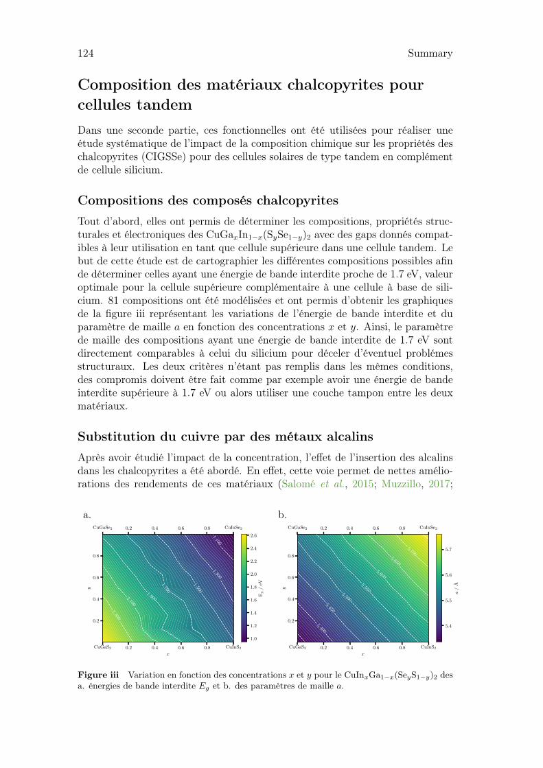
124 Summary
Composition des matériaux chalcopyrites pourcellules tandemDans une seconde partie, ces fonctionnelles ont été utilisées pour réaliser uneétude systématique de l’impact de la composition chimique sur les propriétés deschalcopyrites (CIGSSe) pour des cellules solaires de type tandem en complémentde cellule silicium.
Compositions des composés chalcopyrites
Tout d’abord, elles ont permis de déterminer les compositions, propriétés struc-turales et électroniques des CuGaxIn1−x(SySe1−y)2 avec des gaps donnés compat-ibles à leur utilisation en tant que cellule supérieure dans une cellule tandem. Lebut de cette étude est de cartographier les différentes compositions possibles afinde déterminer celles ayant une énergie de bande interdite proche de 1.7 eV, valeuroptimale pour la cellule supérieure complémentaire à une cellule à base de sili-cium. 81 compositions ont été modélisées et ont permis d’obtenir les graphiquesde la figure iii représentant les variations de l’énergie de bande interdite et duparamètre de maille a en fonction des concentrations x et y. Ainsi, le paramètrede maille des compositions ayant une énergie de bande interdite de 1.7 eV sontdirectement comparables à celui du silicium pour déceler d’éventuel problémesstructuraux. Les deux critères n’étant pas remplis dans les mêmes conditions,des compromis doivent être fait comme par exemple avoir une énergie de bandeinterdite supérieure à 1.7 eV ou alors utiliser une couche tampon entre les deuxmatériaux.
Substitution du cuivre par des métaux alcalins
Après avoir étudié l’impact de la concentration, l’effet de l’insertion des alcalinsdans les chalcopyrites a été abordé. En effet, cette voie permet de nettes amélio-rations des rendements de ces matériaux (Salomé et al., 2015; Muzzillo, 2017;
a. b.
CuGaS2 0.2 0.4 0.6 0.8 CuInS2
x
0.2
0.4
0.6
0.8
y
1.1001.300
1.500
1.700
1.9002.100
2.300
CuGaSe2 0.2 0.4 0.6 0.8 CuInSe2
1.0
1.2
1.4
1.6
1.8
2.0
2.2
2.4
2.6
Eg
/eV
CuGaS2 0.2 0.4 0.6 0.8 CuInS2
x
0.2
0.4
0.6
0.8
y
5.400
5.450
5.500
5.550
5.600
5.650
5.700
CuGaSe2 0.2 0.4 0.6 0.8 CuInSe2
5.4
5.5
5.6
5.7
a/
A
Figure iii Variation en fonction des concentrations x et y pour le CuInxGa1−x(SeyS1−y)2 desa. énergies de bande interdite Eg et b. des paramètres de maille a.
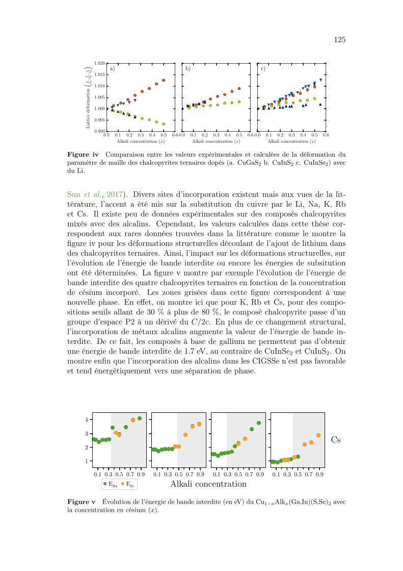
125
0.0 0.1 0.2 0.3 0.4 0.5 0.6
Alkali concentration (x)
0.990
0.995
1.000
1.005
1.010
1.015
1.020
Lat
tice
def
orm
atio
n(a a0,b b 0
,c c 0
) a)
0.0 0.1 0.2 0.3 0.4 0.5 0.6
Alkali concentration (x)
b)
0.0 0.1 0.2 0.3 0.4 0.5 0.6
Alkali concentration (x)
c)
Figure iv Comparaison entre les valeurs expérimentales et calculées de la déformation duparamètre de maille des chalcopyrites ternaires dopés (a. CuGaS2 b. CuInS2 c. CuInSe2) avecdu Li.
Sun et al., 2017). Divers sites d’incorporation existent mais aux vues de la lit-térature, l’accent a été mis sur la substitution du cuivre par le Li, Na, K, Rbet Cs. Il existe peu de données expérimentales sur des composés chalcopyritesmixés avec des alcalins. Cependant, les valeurs calculées dans cette thèse cor-respondent aux rares données trouvées dans la littérature comme le montre lafigure iv pour les déformations structurelles découlant de l’ajout de lithium dansdes chalcopyrites ternaires. Ainsi, l’impact sur les déformations structurelles, surl’évolution de l’énergie de bande interdite ou encore les énergies de subsitutionont été déterminées. La figure v montre par exemple l’évolution de l’énergie debande interdite des quatre chalcopyrites ternaires en fonction de la concentrationde césium incorporé. Les zones grisées dans cette figure correspondent à unenouvelle phase. En effet, on montre ici que pour K, Rb et Cs, pour des compo-sitions seuils allant de 30 % à plus de 80 %, le composé chalcopyrite passe d’ungroupe d’espace P2 à un dérivé du C/2c. En plus de ce changement structural,l’incorporation de métaux alcalins augmente la valeur de l’énergie de bande in-terdite. De ce fait, les composés à base de gallium ne permettent pas d’obtenirune énergie de bande interdite de 1.7 eV, au contraire de CuInSe2 et CuInS2. Onmontre enfin que l’incorporation des alcalins dans les CIGSSe n’est pas favorableet tend énergétiquement vers une séparation de phase.
1
2
3
4
CuGaS2 CuGaSe2 CuInS2 CuInSe2
Li
1
2
3
4
Na
1
2
3
4
Ban
dga
p/
eV
K
1
2
3
4
Rb
0.1 0.3 0.5 0.7 0.9
1
2
3
4
Egd Egi
0.1 0.3 0.5 0.7 0.9
Alkali concentration0.1 0.3 0.5 0.7 0.9 0.1 0.3 0.5 0.7 0.9
Cs
Figure v Évolution de l’énergie de bande interdite (en eV) du Cu1−xAlkx(Ga,In)(S,Se)2 avecla concentration en césium (x).

126 Summary
0.0 0.2 0.4 0.6 0.8 1.0 1.2
µ / eV
−1.0
−0.5
0.0
0.5
1.0
Ef
/eV
H+
H0
H−
Figure vi Variation de l’énergie de formation du H+, H0 et H− dans le silicium avec lepotentiel chimique.
Étude du vieillissement des cellules silicium:importance des défauts ponctuels
Enfin, les défauts ponctuels d’hydrogène, de fer et de bore dans le silicium ont étémodélisés dans le cadre d’une étude préliminaire sur le thème de la dégradationinduite par la lumière à haute temperature (LeTID) qui est l’un des mécanismesde vieillissement des cellules à base de silicium. Cette première étude des défautsponctuels dans le silicium par des fonctionelles hybrides optimisées confirmentles résultats de la littérature (Van de Walle et al., 1989; Brotherton et al., 1985).Pour les défauts d’hydrogène, H+ préfère se placer au centre d’une liaison Si-Si alors que H− se glisse dans les tetrahèdres de la maille. En faisant varier lepotentiel chimique comme sur la figure vi, et comme montré par Van de Walle andNeugebauer (2006), l’hydrogène réagit comme accepteur dans le silicium dopé net donneur dans celui dopé p. H0 correspond quand à lui à un état de transition,instable thermodynamiquement. Le fer et le bore forment de leur côté un centrede recombinaison avec l’apparition d’un niveau d’énergie au centre de la bandeinterdite.
Conclusion
Dans cette thèse, une méthodologie a été adoptée afin d’obtenir des résultatsrapide et précis pour des systèmes complexes. Elle repose sur l’utilisation defonctionnelles hybrides optimisées afin de reproduire les valeurs expérimentalesdes énergies de bandes interdites des matériaux étudiés. Cette approche pragma-tique permet de réduire les erreurs relatives par rapport à l’expérience au niveaucaractéristique standard lors de l’usage des fonctionnelles HSE06 ou M06. Lespropriétés électroniques, telle que les structures en bandes, obtenues via cetteapproche sont comparables à celle calculées par des calculs GW. Cette méthode apar la suite été mise en application pour deux cas concrets relatifs au monde duphotovoltaïque: l’utilisation de matériaux chalcopyrites pour des cellules tandem
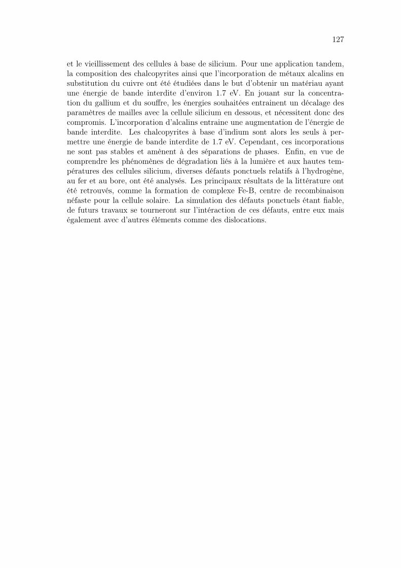
127
et le vieillissement des cellules à base de silicium. Pour une application tandem,la composition des chalcopyrites ainsi que l’incorporation de métaux alcalins ensubstitution du cuivre ont été étudiées dans le but d’obtenir un matériau ayantune énergie de bande interdite d’environ 1.7 eV. En jouant sur la concentra-tion du gallium et du souffre, les énergies souhaitées entrainent un décalage desparamètres de mailles avec la cellule silicium en dessous, et nécessitent donc descompromis. L’incorporation d’alcalins entraine une augmentation de l’énergie debande interdite. Les chalcopyrites à base d’indium sont alors les seuls à per-mettre une énergie de bande interdite de 1.7 eV. Cependant, ces incorporationsne sont pas stables et amènent à des séparations de phases. Enfin, en vue decomprendre les phénomènes de dégradation liés à la lumière et aux hautes tem-pératures des cellules silicium, diverses défauts ponctuels relatifs à l’hydrogène,au fer et au bore, ont été analysés. Les principaux résultats de la littérature ontété retrouvés, comme la formation de complexe Fe-B, centre de recombinaisonnéfaste pour la cellule solaire. La simulation des défauts ponctuels étant fiable,de futurs travaux se tourneront sur l’intéraction de ces défauts, entre eux maiségalement avec d’autres éléments comme des dislocations.

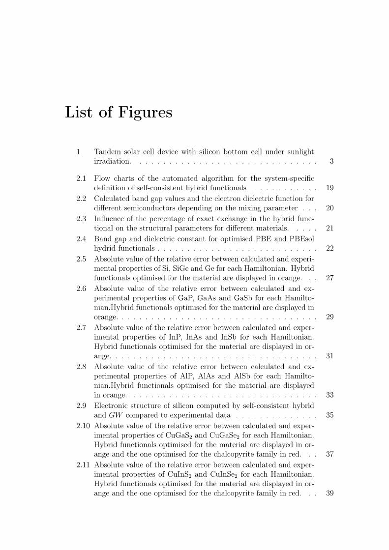
List of Figures
1 Tandem solar cell device with silicon bottom cell under sunlightirradiation. . . . . . . . . . . . . . . . . . . . . . . . . . . . . . . 3
2.1 Flow charts of the automated algorithm for the system-specificdefinition of self-consistent hybrid functionals . . . . . . . . . . . 19
2.2 Calculated band gap values and the electron dielectric function fordifferent semiconductors depending on the mixing parameter . . . 20
2.3 Influence of the percentage of exact exchange in the hybrid func-tional on the structural parameters for different materials. . . . . 21
2.4 Band gap and dielectric constant for optimised PBE and PBEsolhydrid functionals . . . . . . . . . . . . . . . . . . . . . . . . . . . 22
2.5 Absolute value of the relative error between calculated and experi-mental properties of Si, SiGe and Ge for each Hamiltonian. Hybridfunctionals optimised for the material are displayed in orange. . . 27
2.6 Absolute value of the relative error between calculated and ex-perimental properties of GaP, GaAs and GaSb for each Hamilto-nian.Hybrid functionals optimised for the material are displayed inorange. . . . . . . . . . . . . . . . . . . . . . . . . . . . . . . . . . 29
2.7 Absolute value of the relative error between calculated and exper-imental properties of InP, InAs and InSb for each Hamiltonian.Hybrid functionals optimised for the material are displayed in or-ange. . . . . . . . . . . . . . . . . . . . . . . . . . . . . . . . . . . 31
2.8 Absolute value of the relative error between calculated and ex-perimental properties of AlP, AlAs and AlSb for each Hamilto-nian.Hybrid functionals optimised for the material are displayedin orange. . . . . . . . . . . . . . . . . . . . . . . . . . . . . . . . 33
2.9 Electronic structure of silicon computed by self-consistent hybridand GW compared to experimental data . . . . . . . . . . . . . . 35
2.10 Absolute value of the relative error between calculated and exper-imental properties of CuGaS2 and CuGaSe2 for each Hamiltonian.Hybrid functionals optimised for the material are displayed in or-ange and the one optimised for the chalcopyrite family in red. . . 37
2.11 Absolute value of the relative error between calculated and exper-imental properties of CuInS2 and CuInSe2 for each Hamiltonian.Hybrid functionals optimised for the material are displayed in or-ange and the one optimised for the chalcopyrite family in red. . . 39
130 List of Figures
2.12 Electronic structure of various III-V semiconductor computed byself-consistent hybrid and GW compared to experimental data . . 40
2.13 Electronic structure of CuGaSe2 computed by self-consistent hy-brid and GW . . . . . . . . . . . . . . . . . . . . . . . . . . . . . 42
2.14 Temperature dependence of the linear thermal expansion coeffi-cient of various semiconductors . . . . . . . . . . . . . . . . . . . 44
2.15 Temperature influence on the linear thermal expansion coefficienta and c for Cu(In,Ga)(S,Se)2 . . . . . . . . . . . . . . . . . . . . . 45
2.16 Temperature dependence of the band gap of various semiconductors 462.17 Temperature dependence of the band gap of CuGaS2, CuGaSe2,
CuInS2, and CuInSe2 . . . . . . . . . . . . . . . . . . . . . . . . . 472.18 Formation energy of silicon for three different Hamiltonians com-
pared to experimental data . . . . . . . . . . . . . . . . . . . . . . 482.19 Temperature dependence of the heat capacity of Si and GaX (X = P,
As and Sb) . . . . . . . . . . . . . . . . . . . . . . . . . . . . . . 482.20 Electrical conductivity of silicon calculated with different functionals. 492.21 Temperature dependence of the electrical conductivity of silicon. . 502.22 Electrical conductivity of various semiconductors calculated with
the PBEhyb (blue) and PBEsolhyb (orange) functionals. . . . . . . 51
3.1 Chalcopyrite structure of CuBX2 with B = Ga and In, and, X = Sand Se. d, θ1 and θ2 stand for the cation-anion distances and thedifferent angles in the tetrahedra, respectively. . . . . . . . . . . 54
3.2 Flow chart of the method used to determine the different atomicstructures associated to each concentration of complex chalcopyrites. 55
3.3 Band gap and lattice parameters’ variation with the concentrationof CIGSSE . . . . . . . . . . . . . . . . . . . . . . . . . . . . . . . 57
3.4 Comparison of the calculated and experimental variation of theCIGSSE band gap . . . . . . . . . . . . . . . . . . . . . . . . . . 58
3.5 Variation of the binding energy with concentration of CIGSSE . . 593.6 Formation energy’s variation with concentration of CIGSSE . . . 603.7 Comparison between calculated and experimental lattice deforma-
tion in ternary chalcopyrites. . . . . . . . . . . . . . . . . . . . . . 643.8 Lattice deformation of Cu1−xAlkx(Ga,In)(S,Se)2 versus the alkali
concentration . . . . . . . . . . . . . . . . . . . . . . . . . . . . . 663.9 Cu1−xAlkx(Ga,In)(S,Se)2 (Alk = Li, Na, K, Rb, Cs) band gap
evolution (in eV) with the concentration of alkali (x) . . . . . . . 703.10 Bands structures of CuInSe2 and Cu0.75Cs0.25InSe2 in their tetrag-
onal phases . . . . . . . . . . . . . . . . . . . . . . . . . . . . . . 713.11 DOS of Cu0.75Alk0.25InSe2 . . . . . . . . . . . . . . . . . . . . . . 723.12 Substitution energy of Cu by the different alkali (Ef , in eV), as
determined with equation (3.5), including the zero point energy. . 743.13 Formation energies of the mixed phases as given by the reactions A
and B corresponding to the equations (3.7) and (3.8), respectively,including the zero point energy. . . . . . . . . . . . . . . . . . . . 75
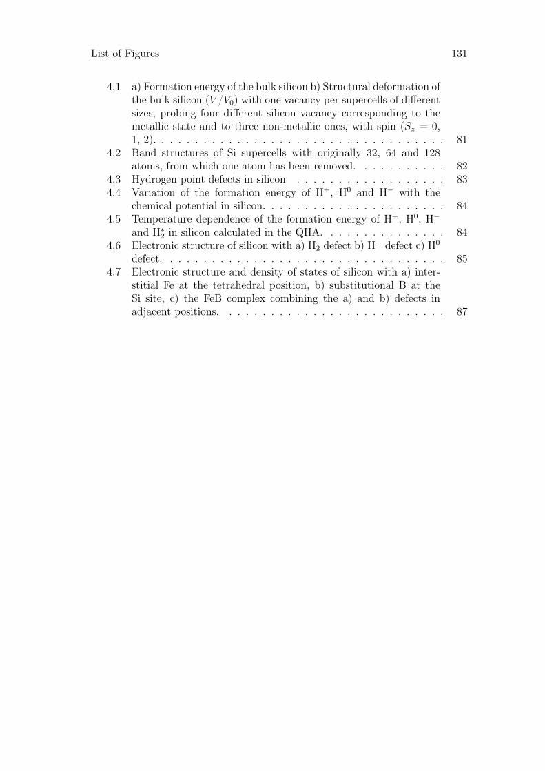
List of Figures 131
4.1 a) Formation energy of the bulk silicon b) Structural deformation ofthe bulk silicon (V /V0) with one vacancy per supercells of differentsizes, probing four different silicon vacancy corresponding to themetallic state and to three non-metallic ones, with spin (Sz = 0,1, 2). . . . . . . . . . . . . . . . . . . . . . . . . . . . . . . . . . . 81
4.2 Band structures of Si supercells with originally 32, 64 and 128atoms, from which one atom has been removed. . . . . . . . . . . 82
4.3 Hydrogen point defects in silicon . . . . . . . . . . . . . . . . . . 834.4 Variation of the formation energy of H+, H0 and H− with the
chemical potential in silicon. . . . . . . . . . . . . . . . . . . . . . 844.5 Temperature dependence of the formation energy of H+, H0, H−
and H∗2 in silicon calculated in the QHA. . . . . . . . . . . . . . . 844.6 Electronic structure of silicon with a) H2 defect b) H− defect c) H0
defect. . . . . . . . . . . . . . . . . . . . . . . . . . . . . . . . . . 854.7 Electronic structure and density of states of silicon with a) inter-
stitial Fe at the tetrahedral position, b) substitutional B at theSi site, c) the FeB complex combining the a) and b) defects inadjacent positions. . . . . . . . . . . . . . . . . . . . . . . . . . . 87

List of Tables
2.1 The performance of two types of self-consistent hybrid Hamiltonians 242.2 Calculated mean absolute relative error in percent between the
calculated and the experimental data for different properties foreach Hamiltonians. . . . . . . . . . . . . . . . . . . . . . . . . . . 24
2.3 Performance of different Hamiltonians on Si, SiGe and Ge properties. 262.4 Performance of different Hamiltonians on GaP, GaAs and GaSb
properties. . . . . . . . . . . . . . . . . . . . . . . . . . . . . . . . 282.5 Performance of different Hamiltonians on InP, InAs and InSb prop-
erties. . . . . . . . . . . . . . . . . . . . . . . . . . . . . . . . . . 302.6 Performance of different Hamiltonians on AlP, AlAs and AlSb
properties. . . . . . . . . . . . . . . . . . . . . . . . . . . . . . . . 322.7 Performance of different Hamiltonians on CuGaS2 and CuGaSe2
properties. . . . . . . . . . . . . . . . . . . . . . . . . . . . . . . . 362.8 Performance of different Hamiltonians on CuInS2 and CuInSe2
properties. . . . . . . . . . . . . . . . . . . . . . . . . . . . . . . . 382.9 Comparison of the hybrid functionals and GW + SO calculated
energies at the Γ point for the III–V semiconductors. . . . . . . . 41
3.1 Construction of the supercells used in the calculations . . . . . . . 653.2 Evolution of the average structure of the anions tetrahedra associ-
ated to each alkali . . . . . . . . . . . . . . . . . . . . . . . . . . . 673.3 Evolution with the alkali of the average structure of the anions
tetrahedra associated to Ga and In . . . . . . . . . . . . . . . . . 683.4 Average Mulliken net atomic charges of alkali and Alk-(S/Se) bond
populations for the different chalcopyrites . . . . . . . . . . . . . . 693.5 Variation of the Cu1−xAlkx(Ga/In)(S/Se)2 (with Alk = Li, Na, K,
Rb and Cs) band gap (in eV) with x varying from 116
to (→) 78. . 71
3.6 Formation energies of Alk(Ga/In)(S/Se)2 with or without secondaryphases from the reactions (3.11) and (3.12), respectively . . . . . 76
4.1 Band gap and formation energy of different impurities after relax-ation . . . . . . . . . . . . . . . . . . . . . . . . . . . . . . . . . . 83
A.1 Exponents of the uncontracted GTFs of Li, Na, K, Rd and Cs . . 137
134 List of Tables
B.1 Reference crystal structure data and the band gap values for thecompounds used for the tests in the present work the substitutionenergy and their structural properties. . . . . . . . . . . . . . . . 139
C.1 Evolution with the alkaline concentration of the average structureof the anions tetrahedra associated to each alkaline for Ga-basedchalcopyrite . . . . . . . . . . . . . . . . . . . . . . . . . . . . . . 142
C.2 Evolution with the alkaline concentration of the average structureof the anions tetrahedra associated to each alkaline for In-basedchalcopyrite . . . . . . . . . . . . . . . . . . . . . . . . . . . . . . 143
C.3 Mulliken net atomic charges of alkali and Alk-(S/Se) bond popu-lations for the different chalcopyrites . . . . . . . . . . . . . . . . 144
C.4 Mulliken net atomic charges of gallium and Ga-(S/Se) bond pop-ulations for the different gallium-based chalcopyrites . . . . . . . . 146
C.5 Mulliken net atomic charges of indium and In-(S/Se) bond popu-lations for the different indium-based chalcopyrites . . . . . . . . 148

Appendices


Appendix A
Basis set
Table A.1 Exponents of the uncontracted GTFs of Li, Na, K, Rd and Cs – see Dovesi et al.(1983, 1991); CRYSTAL17 (2019) for a complete set of data. The K, Rb and Cs basis sets areused in conjunction with the Hay-Wadt small-core pseudoptentials (Hay and Wadt, 1985b,a) .
Atom Shell Expt. Coeff.s(d) p
Li sp 1.466596 1. 1.
sp 0.463406 1. 1.
sp 0.092101 1. 1.
d 0.447768 1.
Na sp 0.517941 1. 1.
sp 0.089944 1. 1.
d 0.162856 1.
K sp 0.310588 1. 1.
sp 0.101487 1. 1.
d 0.525 1.
Rb sp 0.227558 1. 1.
d 0.521716 1.
Cs sp 0.162258 1. 1.
d 0.490609 1.

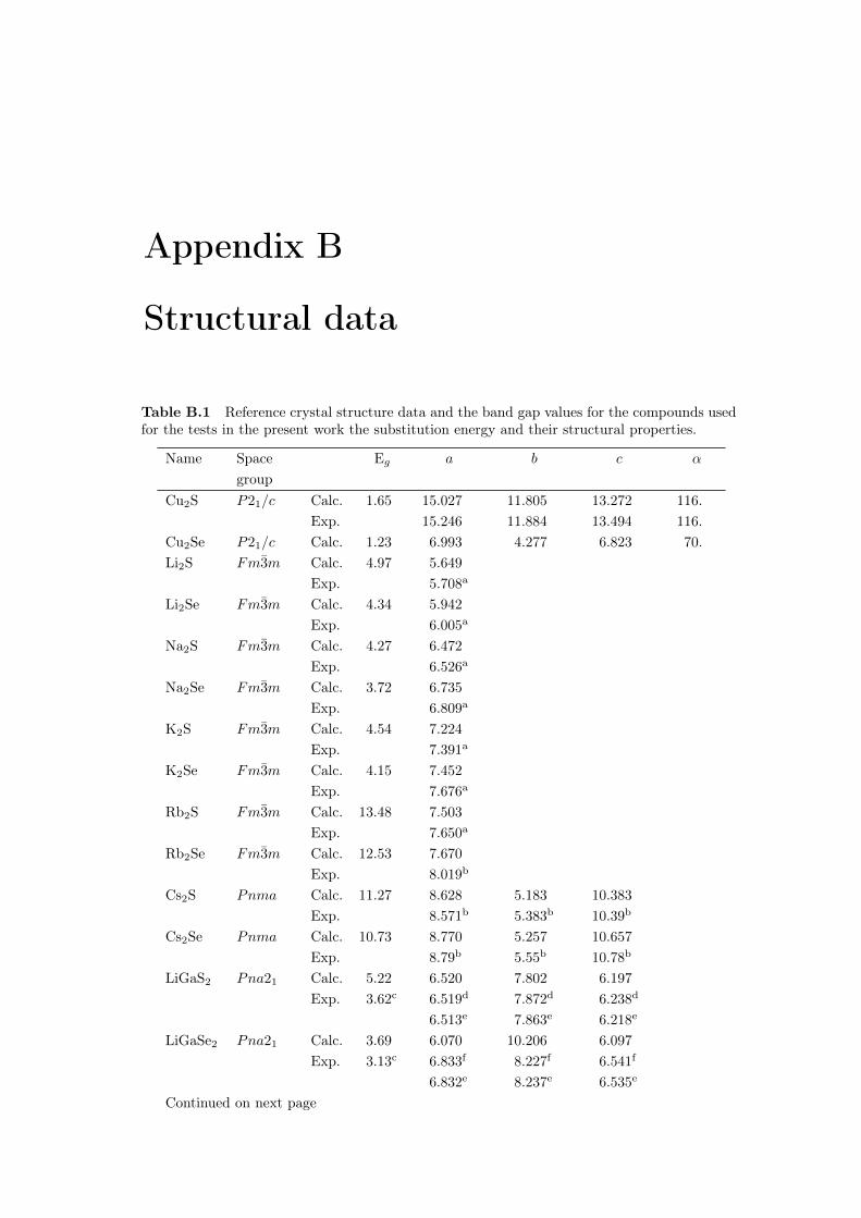
Appendix B
Structural data
Table B.1 Reference crystal structure data and the band gap values for the compounds usedfor the tests in the present work the substitution energy and their structural properties.
Name Space Eg a b c α
groupCu2S P21/c Calc. 1.65 15.027 11.805 13.272 116.
Exp. 15.246 11.884 13.494 116.
Cu2Se P21/c Calc. 1.23 6.993 4.277 6.823 70.
Li2S Fm3m Calc. 4.97 5.649
Exp. 5.708a
Li2Se Fm3m Calc. 4.34 5.942
Exp. 6.005a
Na2S Fm3m Calc. 4.27 6.472
Exp. 6.526a
Na2Se Fm3m Calc. 3.72 6.735
Exp. 6.809a
K2S Fm3m Calc. 4.54 7.224
Exp. 7.391a
K2Se Fm3m Calc. 4.15 7.452
Exp. 7.676a
Rb2S Fm3m Calc. 13.48 7.503
Exp. 7.650a
Rb2Se Fm3m Calc. 12.53 7.670
Exp. 8.019b
Cs2S Pnma Calc. 11.27 8.628 5.183 10.383
Exp. 8.571b 5.383b 10.39b
Cs2Se Pnma Calc. 10.73 8.770 5.257 10.657
Exp. 8.79b 5.55b 10.78b
LiGaS2 Pna21 Calc. 5.22 6.520 7.802 6.197
Exp. 3.62c 6.519d 7.872d 6.238d
6.513e 7.863e 6.218e
LiGaSe2 Pna21 Calc. 3.69 6.070 10.206 6.097
Exp. 3.13c 6.833f 8.227f 6.541f
6.832e 8.237e 6.535e
Continued on next page
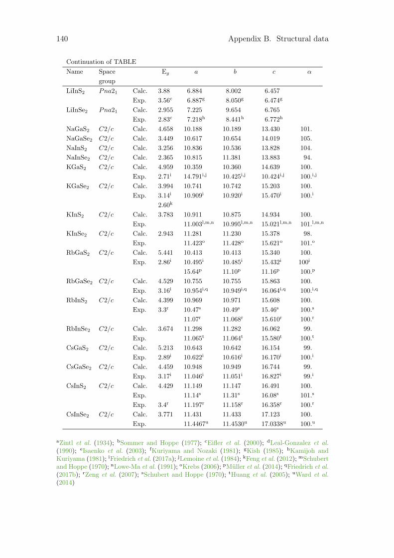
140 Appendix B. Structural data
Continuation of TABLEName Space Eg a b c α
groupLiInS2 Pna21 Calc. 3.88 6.884 8.002 6.457
Exp. 3.56c 6.887g 8.050g 6.474g
LiInSe2 Pna21 Calc. 2.955 7.225 9.654 6.765
Exp. 2.83c 7.218h 8.441h 6.772h
NaGaS2 C2/c Calc. 4.658 10.188 10.189 13.430 101.
NaGaSe2 C2/c Calc. 3.449 10.617 10.654 14.019 105.
NaInS2 C2/c Calc. 3.256 10.836 10.536 13.828 104.
NaInSe2 C2/c Calc. 2.365 10.815 11.381 13.883 94.
KGaS2 C2/c Calc. 4.959 10.359 10.360 14.639 100.
Exp. 2.71i 14.791i,j 10.425i,j 10.424i,j 100.i,j
KGaSe2 C2/c Calc. 3.994 10.741 10.742 15.203 100.
Exp. 3.14i 10.909i 10.920i 15.470i 100.i
2.60k
KInS2 C2/c Calc. 3.783 10.911 10.875 14.934 100.
Exp. 11.003l,m,n 10.995l,m,n 15.021l,m,n 101.l,m,n
KInSe2 C2/c Calc. 2.943 11.281 11.230 15.378 98.
Exp. 11.423o 11.428o 15.621o 101.o
RbGaS2 C2/c Calc. 5.441 10.413 10.413 15.340 100.
Exp. 2.86i 10.495i 10.485i 15.432i 100i
15.64p 11.10p 11.16p 100.p
RbGaSe2 C2/c Calc. 4.529 10.755 10.755 15.863 100.
Exp. 3.16i 10.954i,q 10.949i,q 16.064i,q 100.i,q
RbInS2 C2/c Calc. 4.399 10.969 10.971 15.608 100.
Exp. 3.3r 10.47s 10.49s 15.46s 100.s
11.07r 11.068r 15.610r 100.r
RbInSe2 C2/c Calc. 3.674 11.298 11.282 16.062 99.
Exp. 11.065t 11.064t 15.580t 100.t
CsGaS2 C2/c Calc. 5.213 10.643 10.642 16.154 99.
Exp. 2.89i 10.622i 10.616i 16.170i 100.i
CsGaSe2 C2/c Calc. 4.459 10.948 10.949 16.744 99.
Exp. 3.17i 11.046i 11.051i 16.827i 99.i
CsInS2 C2/c Calc. 4.429 11.149 11.147 16.491 100.
Exp. 11.14s 11.31s 16.08s 101.s
Exp. 3.4r 11.197r 11.158r 16.358r 100.r
CsInSe2 C2/c Calc. 3.771 11.431 11.433 17.123 100.
Exp. 11.4467u 11.4530u 17.0338u 100.u
aZintl et al. (1934); bSommer and Hoppe (1977); cEifler et al. (2000); dLeal-Gonzalez et al.(1990); eIsaenko et al. (2003); fKuriyama and Nozaki (1981); gKish (1985); hKamijoh andKuriyama (1981); iFriedrich et al. (2017a); jLemoine et al. (1984); kFeng et al. (2012); mSchubertand Hoppe (1970); nLowe-Ma et al. (1991); oKrebs (2006); pMüller et al. (2014); qFriedrich et al.(2017b); rZeng et al. (2007); sSchubert and Hoppe (1970); tHuang et al. (2005); uWard et al.(2014)
Appendix C
Alkali incorporation in CIGSSe:supplementary data
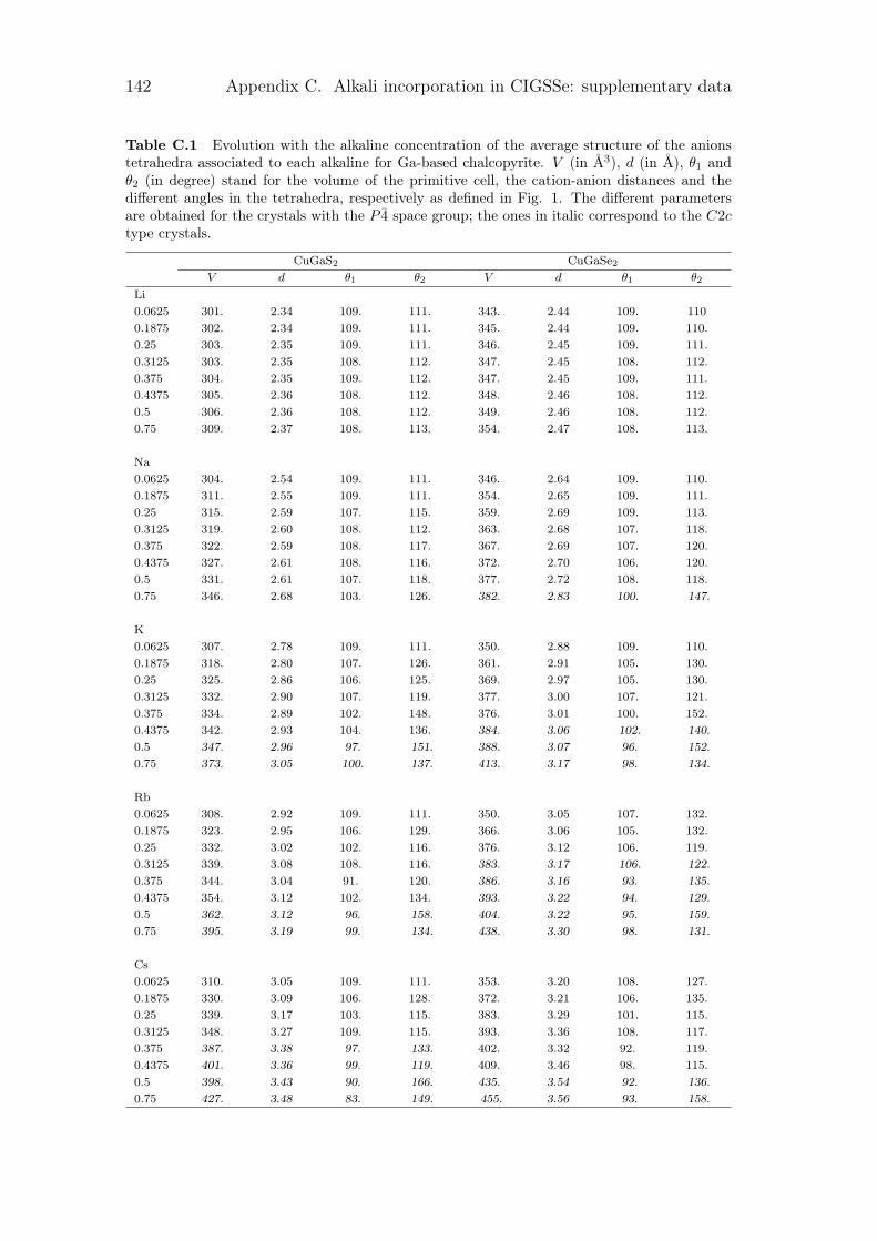
142 Appendix C. Alkali incorporation in CIGSSe: supplementary data
Table C.1 Evolution with the alkaline concentration of the average structure of the anionstetrahedra associated to each alkaline for Ga-based chalcopyrite. V (in Å3), d (in Å), θ1 andθ2 (in degree) stand for the volume of the primitive cell, the cation-anion distances and thedifferent angles in the tetrahedra, respectively as defined in Fig. 1. The different parametersare obtained for the crystals with the P 4 space group; the ones in italic correspond to the C2ctype crystals.
CuGaS2 CuGaSe2V d θ1 θ2 V d θ1 θ2
Li0.0625 301. 2.34 109. 111. 343. 2.44 109. 1100.1875 302. 2.34 109. 111. 345. 2.44 109. 110.0.25 303. 2.35 109. 111. 346. 2.45 109. 111.0.3125 303. 2.35 108. 112. 347. 2.45 108. 112.0.375 304. 2.35 109. 112. 347. 2.45 109. 111.0.4375 305. 2.36 108. 112. 348. 2.46 108. 112.0.5 306. 2.36 108. 112. 349. 2.46 108. 112.0.75 309. 2.37 108. 113. 354. 2.47 108. 113.
Na0.0625 304. 2.54 109. 111. 346. 2.64 109. 110.0.1875 311. 2.55 109. 111. 354. 2.65 109. 111.0.25 315. 2.59 107. 115. 359. 2.69 109. 113.0.3125 319. 2.60 108. 112. 363. 2.68 107. 118.0.375 322. 2.59 108. 117. 367. 2.69 107. 120.0.4375 327. 2.61 108. 116. 372. 2.70 106. 120.0.5 331. 2.61 107. 118. 377. 2.72 108. 118.0.75 346. 2.68 103. 126. 382. 2.83 100. 147.
K0.0625 307. 2.78 109. 111. 350. 2.88 109. 110.0.1875 318. 2.80 107. 126. 361. 2.91 105. 130.0.25 325. 2.86 106. 125. 369. 2.97 105. 130.0.3125 332. 2.90 107. 119. 377. 3.00 107. 121.0.375 334. 2.89 102. 148. 376. 3.01 100. 152.0.4375 342. 2.93 104. 136. 384. 3.06 102. 140.0.5 347. 2.96 97. 151. 388. 3.07 96. 152.0.75 373. 3.05 100. 137. 413. 3.17 98. 134.
Rb0.0625 308. 2.92 109. 111. 350. 3.05 107. 132.0.1875 323. 2.95 106. 129. 366. 3.06 105. 132.0.25 332. 3.02 102. 116. 376. 3.12 106. 119.0.3125 339. 3.08 108. 116. 383. 3.17 106. 122.0.375 344. 3.04 91. 120. 386. 3.16 93. 135.0.4375 354. 3.12 102. 134. 393. 3.22 94. 129.0.5 362. 3.12 96. 158. 404. 3.22 95. 159.0.75 395. 3.19 99. 134. 438. 3.30 98. 131.
Cs0.0625 310. 3.05 109. 111. 353. 3.20 108. 127.0.1875 330. 3.09 106. 128. 372. 3.21 106. 135.0.25 339. 3.17 103. 115. 383. 3.29 101. 115.0.3125 348. 3.27 109. 115. 393. 3.36 108. 117.0.375 387. 3.38 97. 133. 402. 3.32 92. 119.0.4375 401. 3.36 99. 119. 409. 3.46 98. 115.0.5 398. 3.43 90. 166. 435. 3.54 92. 136.0.75 427. 3.48 83. 149. 455. 3.56 93. 158.
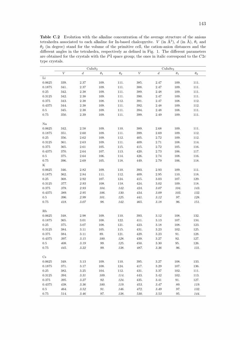
143
Table C.2 Evolution with the alkaline concentration of the average structure of the anionstetrahedra associated to each alkaline for In-based chalcopyrite. V (in Å3), d (in Å), θ1 andθ2 (in degree) stand for the volume of the primitive cell, the cation-anion distances and thedifferent angles in the tetrahedra, respectively as defined in Fig. 1. The different parametersare obtained for the crystals with the P 4 space group; the ones in italic correspond to the C2ctype crystals.
CuInS2 CuInSe2V d θ1 θ2 V d θ1 θ2
Li0.0625 339. 2.37 109. 111. 385. 2.47 109. 111.0.1875 341. 2.37 109. 111. 388. 2.47 109. 111.0.25 342. 2.38 109. 111. 389. 2.48 109. 111.0.3125 342. 2.38 109. 111. 390. 2.47 109. 111.0.375 343. 2.38 108. 112. 391. 2.47 108. 112.0.4375 344. 2.38 109. 111. 392. 2.48 109. 112.0.5 345. 2.38 109. 111. 394. 2.48 108. 111.0.75 350. 2.39 109. 111. 399. 2.49 109. 111.
Na0.0625 342. 2.58 109. 110. 389. 2.68 109. 111.0.1875 351. 2.60 109. 111. 399. 2.69 109. 112.0.25 356. 2.62 109. 112. 405. 2.72 109. 112.0.3125 361. 2.63 109. 111. 409. 2.71 108. 114.0.375 365. 2.61 105. 115. 415. 2.72 105. 116.0.4375 370. 2.64 107. 113. 420. 2.73 106. 117.0.5 375. 2.64 106. 114. 426. 2.74 108. 116.0.75 396. 2.69 105. 118. 449. 2.79 106. 118.K0.0625 346. 2.82 109. 110. 393. 2.93 109. 111.0.1875 362. 2.84 111. 112. 409. 2.95 110. 118.0.25 368. 2.92 107. 124. 415. 3.03 107. 129.0.3125 377. 2.93 108. 118. 424. 3.02 109. 118.0.375 378. 2.93 104. 142. 424. 3.07 104. 143.0.4375 389. 2.95 106. 130. 434. 3.09 103. 132.0.5 396. 2.99 101. 125. 441. 3.12 97. 128.0.75 418. 3.07 98. 142. 465. 3.18 96. 151.
Rb0.0625 348. 2.98 109. 110. 393. 3.12 108. 132.0.1875 365. 3.01 108. 122. 411. 3.13 107. 134.0.25 375. 3.07 108. 121. 423. 3.18 108. 123.0.3125 384. 3.11 105. 115. 431. 3.23 102. 125.0.375 384. 3.11 89. 121. 429. 3.23 91. 128.0.4375 397. 3.15 100. 128. 439. 3.27 92. 127.0.5 408. 3.19 99. 125. 450. 3.30 95. 126.0.75 445. 3.22 99. 138. 487. 3.36 96. 131.
Cs0.0625 349. 3.13 109. 110. 395. 3.27 108. 133.0.1875 371. 3.17 108. 124. 417. 3.29 107. 136.0.25 382. 3.25 104. 112. 431. 3.37 102. 111.0.3125 394. 3.31 109. 114. 443. 3.42 102. 113.0.375 395. 3.27 92. 124. 435. 3.41 91. 127.0.4375 438. 3.36 100. 119. 453. 3.47 89. 119.0.5 464. 3.52 91. 146. 472. 3.49 97. 132.0.75 514. 3.46 97. 138. 530. 3.53 95. 144.

144 Appendix C. Alkali incorporation in CIGSSe: supplementary data
Table C.3 Mulliken net atomic charges of alkali (q) and Alk-(S/Se) bond populations(bAlk−(S/Se)) for the different chalcopyrites. The data for Cu in Cu(Ga/In)(S/Se)2 (referencedas Cu) are given for comparison.
Alk. CuGaS2 CuGaSe2 CuInS2 CuInSe2q bAlk−S q bAlk−S q bAlk−S q bAlk−S
Li0.0625 +0.411 +0.1883 +0.226 +0.256 +0.404 +0.228 +0.221 +0.284
0.125 +0.414 +0.1884 +0.227 +0.254 +0.405 +0.228 +0.222 +0.284
0.1875 +0.410 +0.1894 +0.224 +0.255 +0.402 +0.228 +0.220 +0.286
0.25 +0.407 +0.1926 +0.224 +0.258 +0.402 +0.229 +0.220 +0.286
0.3125 +0.386 +0.1944 +0.202 +0.258 +0.389 +0.230 +0.207 +0.286
0.375 +0.391 +0.1937 +0.205 +0.258 +0.392 +0.230 +0.210 +0.287
0.4375 +0.376 +0.1963 +0.191 +0.259 +0.383 +0.232 +0.201 +0.287
0.5 +0.381 +0.1969 +0.196 +0.259 +0.385 +0.232 +0.204 +0.287
0.625 +0.386 +0.1955 +0.201 +0.258 +0.389 +0.232 +0.207 +0.288
0.75 +0.370 +0.1985 +0.186 +0.260 +0.379 +0.234 +0.199 +0.289
0.875 +0.361 +0.1992 +0.177 +0.261 +0.373 +0.235 +0.193 +0.289
Na0.0625 +0.439 +0.1680 +0.284 +0.224 +0.433 +0.196 +0.283 +0.246
0.125 +0.444 +0.1622 +0.278 +0.224 +0.433 +0.196 +0.279 +0.246
0.1875 +0.438 +0.1680 +0.279 +0.225 +0.430 +0.198 +0.280 +0.247
0.25 +0.437 +0.1708 +0.289 +0.223 +0.435 +0.198 +0.291 +0.244
0.3125 +0.428 +0.1727 +0.264 +0.229 +0.432 +0.198 +0.266 +0.250
0.375 +0.412 +0.1752 +0.264 +0.227 +0.418 +0.203 +0.273 +0.249
0.4375 +0.411 +0.1777 +0.249 +0.233 +0.417 +0.204 +0.257 +0.254
0.5 +0.403 +0.1809 +0.257 +0.230 +0.408 +0.206 +0.264 +0.252
0.625 +0.411 +0.1749 +0.268 +0.218 +0.416 +0.204 +0.272 +0.249
0.75 +0.389 +0.1797 +0.225 +0.190 +0.403 +0.207 +0.267 +0.248
0.875 +0.346 +0.1485 +0.209 +0.169 +0.398 +0.205 +0.267 +0.168
K0.0625 +0.712 +0.0127 +0.624 +0.060 +0.734 +0.030 +0.646 +0.076
0.125 +0.717 −0.003 +0.629 +0.042 +0.731 +0.020 +0.661 +0.061
0.1875 +0.709 +0.0137 +0.619 +0.058 +0.730 +0.033 +0.649 +0.075
0.25 +0.709 +0.0319 +0.624 +0.065 +0.736 +0.041 +0.653 +0.072
0.3125 +0.702 +0.0375 +0.618 +0.070 +0.732 +0.045 +0.628 +0.088
0.375 +0.683 +0.0373 +0.591 +0.068 +0.718 +0.046 +0.639 +0.073
0.4375 +0.683 +0.0437 +0.591 +0.071 +0.719 +0.051 +0.642 +0.080
0.5 +0.655 +0.0528 +0.567 +0.075 +0.703 +0.058 +0.620 +0.083
0.625 +0.659 +0.0589 +0.589 +0.067 +0.689 +0.061 +0.619 +0.074
0.75 +0.649 +0.0628 +0.562 +0.085 +0.683 +0.062 +0.602 +0.087
0.875 +0.627 +0.0633 +0.540 +0.081 +0.671 +0.067 +0.591 +0.087
Rb0.0625 +1.049 −0.082 +1.035 −0.056 +1.037 −0.066 +1.027 −0.043
Continued on next page
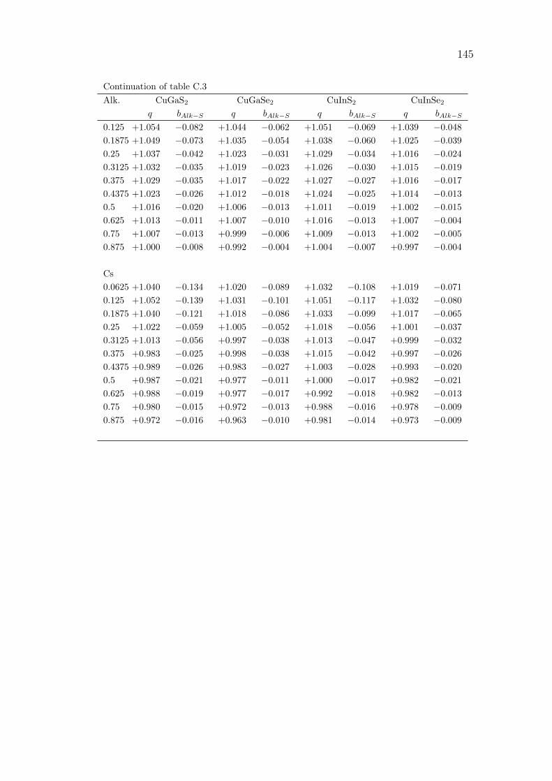
145
Continuation of table C.3Alk. CuGaS2 CuGaSe2 CuInS2 CuInSe2
q bAlk−S q bAlk−S q bAlk−S q bAlk−S0.125 +1.054 −0.082 +1.044 −0.062 +1.051 −0.069 +1.039 −0.048
0.1875 +1.049 −0.073 +1.035 −0.054 +1.038 −0.060 +1.025 −0.039
0.25 +1.037 −0.042 +1.023 −0.031 +1.029 −0.034 +1.016 −0.024
0.3125 +1.032 −0.035 +1.019 −0.023 +1.026 −0.030 +1.015 −0.019
0.375 +1.029 −0.035 +1.017 −0.022 +1.027 −0.027 +1.016 −0.017
0.4375 +1.023 −0.026 +1.012 −0.018 +1.024 −0.025 +1.014 −0.013
0.5 +1.016 −0.020 +1.006 −0.013 +1.011 −0.019 +1.002 −0.015
0.625 +1.013 −0.011 +1.007 −0.010 +1.016 −0.013 +1.007 −0.004
0.75 +1.007 −0.013 +0.999 −0.006 +1.009 −0.013 +1.002 −0.005
0.875 +1.000 −0.008 +0.992 −0.004 +1.004 −0.007 +0.997 −0.004
Cs0.0625 +1.040 −0.134 +1.020 −0.089 +1.032 −0.108 +1.019 −0.071
0.125 +1.052 −0.139 +1.031 −0.101 +1.051 −0.117 +1.032 −0.080
0.1875 +1.040 −0.121 +1.018 −0.086 +1.033 −0.099 +1.017 −0.065
0.25 +1.022 −0.059 +1.005 −0.052 +1.018 −0.056 +1.001 −0.037
0.3125 +1.013 −0.056 +0.997 −0.038 +1.013 −0.047 +0.999 −0.032
0.375 +0.983 −0.025 +0.998 −0.038 +1.015 −0.042 +0.997 −0.026
0.4375 +0.989 −0.026 +0.983 −0.027 +1.003 −0.028 +0.993 −0.020
0.5 +0.987 −0.021 +0.977 −0.011 +1.000 −0.017 +0.982 −0.021
0.625 +0.988 −0.019 +0.977 −0.017 +0.992 −0.018 +0.982 −0.013
0.75 +0.980 −0.015 +0.972 −0.013 +0.988 −0.016 +0.978 −0.009
0.875 +0.972 −0.016 +0.963 −0.010 +0.981 −0.014 +0.973 −0.009
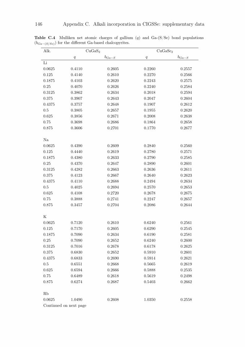
146 Appendix C. Alkali incorporation in CIGSSe: supplementary data
Table C.4 Mulliken net atomic charges of gallium (q) and Ga-(S/Se) bond populations(bGa−(S/Se)) for the different Ga-based chalcopyrites.
Alk. CuGaS2 CuGaSe2q bGa−S q bGa−S
Li0.0625 0.4110 0.2605 0.2260 0.2557
0.125 0.4140 0.2610 0.2270 0.2566
0.1875 0.4103 0.2620 0.2243 0.2575
0.25 0.4070 0.2626 0.2240 0.2584
0.3125 0.3862 0.2634 0.2018 0.2594
0.375 0.3907 0.2643 0.2047 0.2604
0.4375 0.3757 0.2648 0.1907 0.2612
0.5 0.3805 0.2657 0.1955 0.2620
0.625 0.3856 0.2671 0.2008 0.2638
0.75 0.3698 0.2686 0.1864 0.2658
0.875 0.3606 0.2701 0.1770 0.2677
Na0.0625 0.4390 0.2609 0.2840 0.2560
0.125 0.4440 0.2619 0.2780 0.2571
0.1875 0.4380 0.2633 0.2790 0.2585
0.25 0.4370 0.2647 0.2890 0.2601
0.3125 0.4282 0.2663 0.2636 0.2611
0.375 0.4123 0.2667 0.2640 0.2623
0.4375 0.4110 0.2688 0.2494 0.2634
0.5 0.4025 0.2694 0.2570 0.2653
0.625 0.4108 0.2720 0.2678 0.2675
0.75 0.3888 0.2741 0.2247 0.2657
0.875 0.3457 0.2704 0.2086 0.2644
K0.0625 0.7120 0.2610 0.6240 0.2561
0.125 0.7170 0.2605 0.6290 0.2545
0.1875 0.7090 0.2634 0.6190 0.2581
0.25 0.7090 0.2652 0.6240 0.2600
0.3125 0.7016 0.2678 0.6178 0.2625
0.375 0.6830 0.2652 0.5910 0.2601
0.4375 0.6833 0.2690 0.5914 0.2621
0.5 0.6551 0.2668 0.5665 0.2619
0.625 0.6594 0.2666 0.5888 0.2535
0.75 0.6489 0.2618 0.5619 0.2498
0.875 0.6274 0.2687 0.5403 0.2662
Rb0.0625 1.0490 0.2608 1.0350 0.2558
Continued on next page
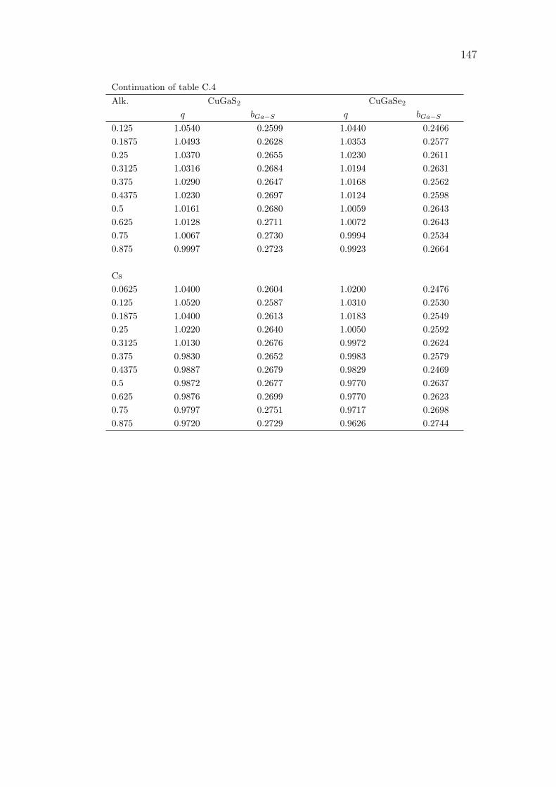
147
Continuation of table C.4Alk. CuGaS2 CuGaSe2
q bGa−S q bGa−S0.125 1.0540 0.2599 1.0440 0.2466
0.1875 1.0493 0.2628 1.0353 0.2577
0.25 1.0370 0.2655 1.0230 0.2611
0.3125 1.0316 0.2684 1.0194 0.2631
0.375 1.0290 0.2647 1.0168 0.2562
0.4375 1.0230 0.2697 1.0124 0.2598
0.5 1.0161 0.2680 1.0059 0.2643
0.625 1.0128 0.2711 1.0072 0.2643
0.75 1.0067 0.2730 0.9994 0.2534
0.875 0.9997 0.2723 0.9923 0.2664
Cs0.0625 1.0400 0.2604 1.0200 0.2476
0.125 1.0520 0.2587 1.0310 0.2530
0.1875 1.0400 0.2613 1.0183 0.2549
0.25 1.0220 0.2640 1.0050 0.2592
0.3125 1.0130 0.2676 0.9972 0.2624
0.375 0.9830 0.2652 0.9983 0.2579
0.4375 0.9887 0.2679 0.9829 0.2469
0.5 0.9872 0.2677 0.9770 0.2637
0.625 0.9876 0.2699 0.9770 0.2623
0.75 0.9797 0.2751 0.9717 0.2698
0.875 0.9720 0.2729 0.9626 0.2744
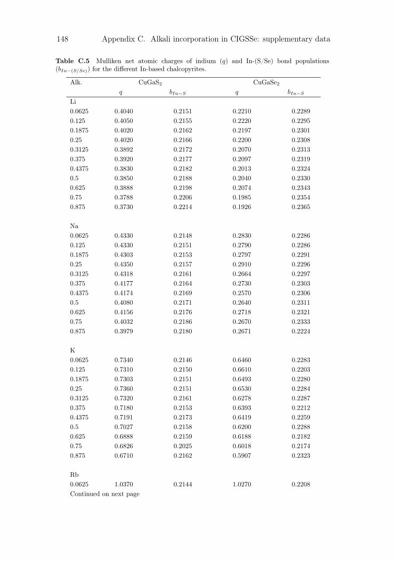
148 Appendix C. Alkali incorporation in CIGSSe: supplementary data
Table C.5 Mulliken net atomic charges of indium (q) and In-(S/Se) bond populations(bIn−(S/Se)) for the different In-based chalcopyrites.
Alk. CuGaS2 CuGaSe2q bIn−S q bIn−S
Li0.0625 0.4040 0.2151 0.2210 0.2289
0.125 0.4050 0.2155 0.2220 0.2295
0.1875 0.4020 0.2162 0.2197 0.2301
0.25 0.4020 0.2166 0.2200 0.2308
0.3125 0.3892 0.2172 0.2070 0.2313
0.375 0.3920 0.2177 0.2097 0.2319
0.4375 0.3830 0.2182 0.2013 0.2324
0.5 0.3850 0.2188 0.2040 0.2330
0.625 0.3888 0.2198 0.2074 0.2343
0.75 0.3788 0.2206 0.1985 0.2354
0.875 0.3730 0.2214 0.1926 0.2365
Na0.0625 0.4330 0.2148 0.2830 0.2286
0.125 0.4330 0.2151 0.2790 0.2286
0.1875 0.4303 0.2153 0.2797 0.2291
0.25 0.4350 0.2157 0.2910 0.2296
0.3125 0.4318 0.2161 0.2664 0.2297
0.375 0.4177 0.2164 0.2730 0.2303
0.4375 0.4174 0.2169 0.2570 0.2306
0.5 0.4080 0.2171 0.2640 0.2311
0.625 0.4156 0.2176 0.2718 0.2321
0.75 0.4032 0.2186 0.2670 0.2333
0.875 0.3979 0.2180 0.2671 0.2224
K0.0625 0.7340 0.2146 0.6460 0.2283
0.125 0.7310 0.2150 0.6610 0.2203
0.1875 0.7303 0.2151 0.6493 0.2280
0.25 0.7360 0.2151 0.6530 0.2284
0.3125 0.7320 0.2161 0.6278 0.2287
0.375 0.7180 0.2153 0.6393 0.2212
0.4375 0.7191 0.2173 0.6419 0.2259
0.5 0.7027 0.2158 0.6200 0.2288
0.625 0.6888 0.2159 0.6188 0.2182
0.75 0.6826 0.2025 0.6018 0.2174
0.875 0.6710 0.2162 0.5907 0.2323
Rb0.0625 1.0370 0.2144 1.0270 0.2208
Continued on next page
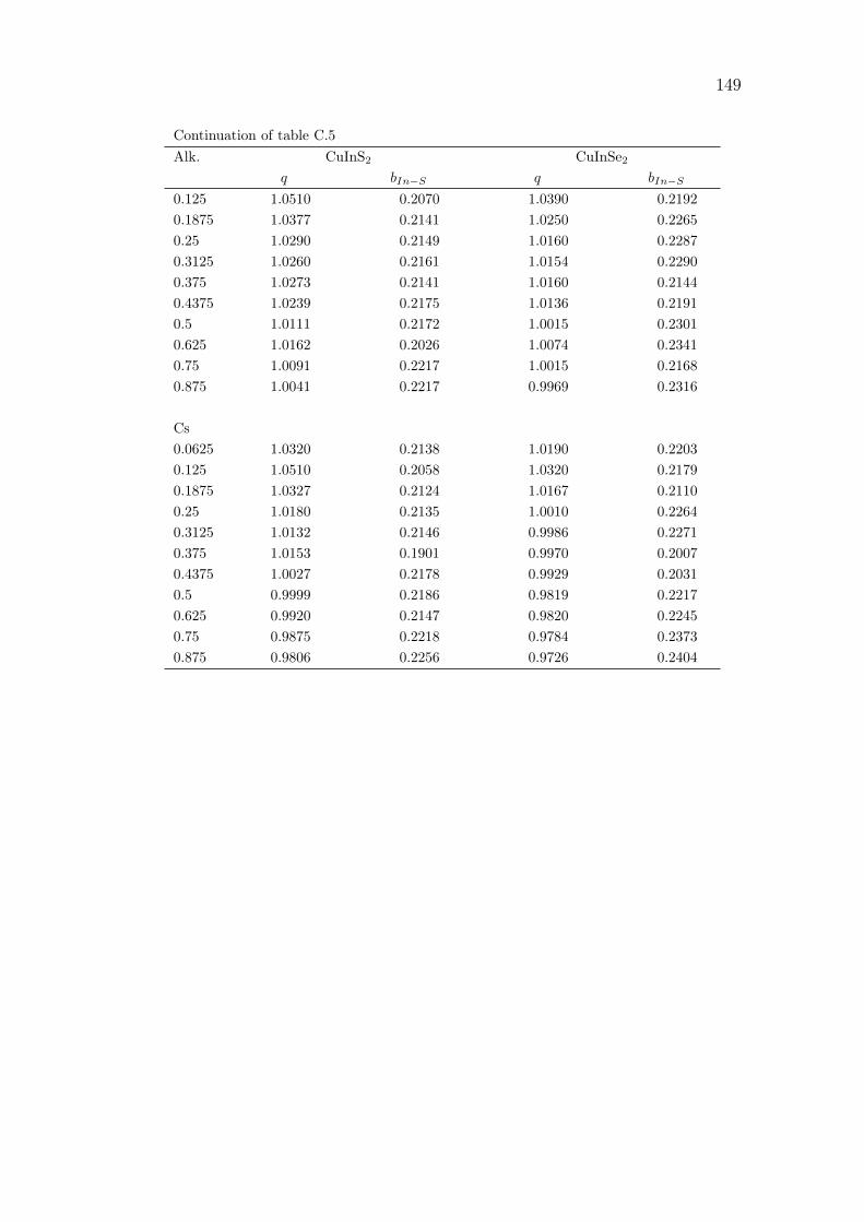
149
Continuation of table C.5Alk. CuInS2 CuInSe2
q bIn−S q bIn−S0.125 1.0510 0.2070 1.0390 0.2192
0.1875 1.0377 0.2141 1.0250 0.2265
0.25 1.0290 0.2149 1.0160 0.2287
0.3125 1.0260 0.2161 1.0154 0.2290
0.375 1.0273 0.2141 1.0160 0.2144
0.4375 1.0239 0.2175 1.0136 0.2191
0.5 1.0111 0.2172 1.0015 0.2301
0.625 1.0162 0.2026 1.0074 0.2341
0.75 1.0091 0.2217 1.0015 0.2168
0.875 1.0041 0.2217 0.9969 0.2316
Cs0.0625 1.0320 0.2138 1.0190 0.2203
0.125 1.0510 0.2058 1.0320 0.2179
0.1875 1.0327 0.2124 1.0167 0.2110
0.25 1.0180 0.2135 1.0010 0.2264
0.3125 1.0132 0.2146 0.9986 0.2271
0.375 1.0153 0.1901 0.9970 0.2007
0.4375 1.0027 0.2178 0.9929 0.2031
0.5 0.9999 0.2186 0.9819 0.2217
0.625 0.9920 0.2147 0.9820 0.2245
0.75 0.9875 0.2218 0.9784 0.2373
0.875 0.9806 0.2256 0.9726 0.2404