Page i

HYBRID MASONRY CONNECTOR DEVELOPMENT

PHASE II

Reef Ozaki-Train Gaur Johnson

and Ian N. Robertson

Research Report UHM/CEE/11-04 December 2011

Page ii

Page iii

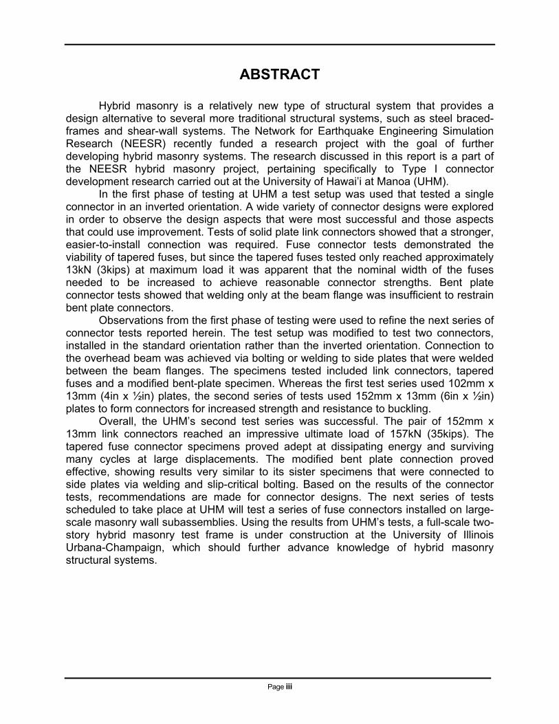
ABSTRACT Hybrid masonry is a relatively new type of structural system that provides a design alternative to several more traditional structural systems, such as steel braced-frames and shear-wall systems. The Network for Earthquake Engineering Simulation Research (NEESR) recently funded a research project with the goal of further developing hybrid masonry systems. The research discussed in this report is a part of the NEESR hybrid masonry project, pertaining specifically to Type I connector development research carried out at the University of Hawai’i at Manoa (UHM). In the first phase of testing at UHM a test setup was used that tested a single connector in an inverted orientation. A wide variety of connector designs were explored in order to observe the design aspects that were most successful and those aspects that could use improvement. Tests of solid plate link connectors showed that a stronger, easier-to-install connection was required. Fuse connector tests demonstrated the viability of tapered fuses, but since the tapered fuses tested only reached approximately 13kN (3kips) at maximum load it was apparent that the nominal width of the fuses needed to be increased to achieve reasonable connector strengths. Bent plate connector tests showed that welding only at the beam flange was insufficient to restrain bent plate connectors.

Observations from the first phase of testing were used to refine the next series of connector tests reported herein. The test setup was modified to test two connectors, installed in the standard orientation rather than the inverted orientation. Connection to the overhead beam was achieved via bolting or welding to side plates that were welded between the beam flanges. The specimens tested included link connectors, tapered fuses and a modified bent-plate specimen. Whereas the first test series used 102mm x 13mm (4in x ½in) plates, the second series of tests used 152mm x 13mm (6in x ½in) plates to form connectors for increased strength and resistance to buckling.

Overall, the UHM’s second test series was successful. The pair of 152mm x 13mm link connectors reached an impressive ultimate load of 157kN (35kips). The tapered fuse connector specimens proved adept at dissipating energy and surviving many cycles at large displacements. The modified bent plate connection proved effective, showing results very similar to its sister specimens that were connected to side plates via welding and slip-critical bolting. Based on the results of the connector tests, recommendations are made for connector designs. The next series of tests scheduled to take place at UHM will test a series of fuse connectors installed on large-scale masonry wall subassemblies. Using the results from UHM’s tests, a full-scale two-story hybrid masonry test frame is under construction at the University of Illinois Urbana-Champaign, which should further advance knowledge of hybrid masonry structural systems.

Page iv

ACKNOWLEDGEMENTS

This report is based on research and testing conducted under the direction of

Drs. Ian Robertson and Gaur Johnson. The authors would like to thank Drs. Ronald

Riggs and David Ma for their contributions as part of the Thesis Committee for the

project.

Special thanks go to Mitchell Pinkerton and Miles Wagner of the University of

Hawai‘i at Mānoa’s Structural Testing Laboratory for their assistance throughout the

project. The authors would also like to thank graduate researcher Steven Mitsuyuki for

his assistance with testing.

This research was supported by the National Science Foundation under Grant

No. CMMI 0936464 as part of the George E. Brown, Jr. Network for Earthquake

Engineering Simulation. This support is gratefully acknowledged.

Page v

TABLE OF CONTENTS

ABSTRACT ................................................................................................................... iii

ACKNOWLEDGEMENTS .............................................................................................. iv

1 INTRODUCTION ...................................................................................................... 1

1.1 INTRODUCTION ..................................................................................................... 1 1.2 OBJECTIVE ........................................................................................................... 1

2 LITERATURE REVIEW ............................................................................................ 3

2.1 HYBRID MASONRY LATERAL LOAD RESISTING SYSTEM ............................................ 3 2.2 CONNECTOR PLATES ............................................................................................ 4 2.3 UHM RESEARCH .................................................................................................. 6

2.3.1 Connector Plates ................................................................................................................... 6 2.3.2 Bolt Push Out Tests .............................................................................................................. 7

3 MATERIAL PROPERTIES ....................................................................................... 9

3.1 TENSION TESTS .................................................................................................... 9 3.1.1 Motivation .............................................................................................................................. 9 3.1.2 Experimental Setup ............................................................................................................... 9 3.1.3 Test Specimens ..................................................................................................................... 9 3.1.4 Test Procedure .................................................................................................................... 10

3.2 TENSION TEST RESULTS ..................................................................................... 10

4 APPROACH ........................................................................................................... 13

4.1 DOUBLE SIDE PLATE CONNECTOR TESTING .......................................................... 13 4.1.1 Experimental Setup ............................................................................................................. 13 4.1.2 Test Specimens ................................................................................................................... 16 4.1.3 Procedure – Tapered fuse connector design ...................................................................... 20 4.1.4 Procedure – Theoretical Yield Points and Ultimate Load Calculations ............................... 25 4.1.5 Procedure – Double side plate connector testing ............................................................... 29

4.2 FULL-SCALE STEEL-MASONRY SUBASSEMBLIES ................................................... 31

5 RESULTS ............................................................................................................... 33

5.1 DOUBLE SIDE-PLATE SHEAR CONNECTOR TESTS .................................................. 33 5.1.1 Theoretical Results.............................................................................................................. 33 5.1.2 Load-Displacement Hysteretic Diagrams and Specimen Narratives .................................. 33

5.1.2.1 S-P4_T4-01 ................................................................................................................................... 34 5.1.2.2 S-P6_T4_FT2-01 ........................................................................................................................... 35 5.1.2.3 S-P6_T4-01 ................................................................................................................................... 37 5.1.2.4 S-P6_T4_FT2.4 -01 ....................................................................................................................... 38 5.1.2.5 S-P6_T4_FT2.4_W-01 .................................................................................................................. 39 5.1.2.6 S-P6_T4_FT2.4_BP-01 ................................................................................................................. 41

5.1.3 Vertical Load (Load Rod) Hysteretic Diagrams ................................................................... 42 5.1.4 Critical values from hysteretic plots ..................................................................................... 43

6 ANALYSIS ............................................................................................................. 45

6.1 COMPARISON OF PREDICTED RESULTS VS. EXPERIMENTAL RESULTS ..................... 45 6.2 COMPARISON OF SIDE-PLATE CONNECTORS .......................................................... 47

6.2.1 Comparison of Link vs. Fuse Connectors ........................................................................... 47

Page vi

6.2.2 Comparison of side-plate connection methods ................................................................... 48 6.3 ATC-24 CONNECTOR PLATE ANALYSIS ................................................................ 49

7 CONCLUSIONS / RECOMMENDATIONS ............................................................. 53

8 REFERENCES ....................................................................................................... 55

A1: DTI WASHERS PRODUCT SPECIFICATION ..................................................... A-2

A2: TENSION TEST STRESS-STRAIN CURVES ...................................................... A-3

½” PLATE (FROM 4” WIDE STOCK) ................................................................................. A-3 ½” PLATE (FROM 6” WIDE STOCK) ................................................................................. A-4

A3: CONNECTOR YIELD FORCE CALCULATIONS SPREADSHEET .................... A-5

A4: CONNECTOR YIELD DISPLACEMENT CALCULATIONS SPREADSHEET ..... A-5

A5: CONNECTOR ULTIMATE FORCE CALCULATIONS SPREADSHEETS .......... A-6

A6: LOAD-DISPLACEMENT HYSTERETIC PLOTS IN US CUSTOMARY UNITS ... A-8

A7: VERTICAL LOAD VS. SHEAR LOAD HYSTERETIC PLOTS ............................ A-9

A8: ATC-24 SPREADSHEETS ................................................................................. A-10

Page vii

LIST OF FIGURES

Figure 2-1: Hybrid Masonry Types I, II, and III, shown clockwise from top left ................ 3

Figure 2-2: Type I Hybrid Masonry Wall [IMI, 2011] ........................................................ 4

Figure 2-3: Connector plate detailing requirements [IMI, 2011] ....................................... 5

Figure 2-4: Diagrams of various connector types tested ................................................. 6

Figure 2-5: Bolt push out test schematic ......................................................................... 8

Figure 3-1: Typical tension specimen in the testing frame .............................................. 9

Figure 3-2: Typical Tension Specimen Diagram ........................................................... 10

Figure 4-1: Old, single connector plate test setup ......................................................... 13

Figure 4-2: Modified HSS-W12 upper portion of test setup ........................................... 14

Figure 4-3: Upper test setup modifications and bottom plate. ....................................... 15

Figure 4-4: Final bottom plate, removed from bottom portion of test setup ................... 15

Figure 4-5: Double side plate connecter test setup ....................................................... 16

Figure 4-6: Link Connector Specimens: (a) S-P4_T4-01; (b) S-P6_T4-01 .................... 18

Figure 4-7: Flat Plate Fuse Specimens: (a) S-P6_T4_FT2-01; (b) S-P6_T4_FT2.4-01; (c) S-P6_T4_FT2.4_W-01. ....................................................................................... 19

Figure 4-8: (a) Detail of S-P6_T4_FT2.4_BP-01; (b) Section A-A; (c) Specimen in test setup ........................................................................................................................ 20

Figure 4-9: Tapered Fuse Connector Properties Diagram ............................................ 21

Figure 4-10: Fuse connector design diagrams (a) Bolted; (b) Welded .......................... 23

Figure 4-11: (a) Bent Plate Design Diagrams; (b) FBD: Moments about Y’ .................. 24

Figure 4-12: S-P6_T4-01: Diagram for Theoretical Calculations ................................... 26

Figure 4-13: Section a-a (Figure 4-12) Moment of Inertia calculated by parts ............... 26

Figure 4-14: S-P6_T4-01: Displacement Integration Diagram ....................................... 27

Figure 4-15: Modified ATC-24 cyclic loading routine for steel connector plates ............ 30

Page viii

Figure 4-16: Large-scale steel-masonry subassembly test setup ................................. 32

Figure 4-17: Graphic representation of the proposed full-scale test structure to be constructed at UIUC ................................................................................................. 32

Figure 5-1: S-P4_T4-01: (a) Thru-bolt failure detail; (b) plate specimens post-testing .. 34

Figure 5-2: Load-Displacement hysteretic diagram for S-P4_T4-01 ............................. 35

Figure 5-3: Load-Displacement Hysteretic Diagram for S-P6_T4_FT2-01 .................... 36

Figure 5-4: Torsional buckling of S-P6_T4_FT2-01 at ±70mm ...................................... 36

Figure 5-5: Load-Displacement hysteretic diagram for S-P6_T4-01 ............................. 37

Figure 5-6: S-P6_T4-01 (a) Initial view; (b) Failed connectors, side-by-side ................. 38

Figure 5-7: Load-Displacement hysteretic diagram for S-P6_T4_FT2.4-01 .................. 38

Figure 5-8: (a) Mid-routine specimen view; (b) Failed connectors side-by-side ............ 39

Figure 5-9: Load-Displacement hysteretic diagram for S-P6_T4_FT2.4_W-01 ............. 40

Figure 5-10: S-P6_T4_FT2.4_W-01: Failed connectors side-by-side ........................... 40

Figure 5-11: Load-Displacement hysteretic diagram for S-P6_T4_FT2.4_BP-01 ......... 41

Figure 5-12: S-P6_T4_FT2.4_BP-01: Failure of the back connector ............................ 41

Figure 5-13: Vertical and Shear Load vs. Displacement Hystereses: ........................... 42

Page ix

LIST OF TABLES

Table 2-1: Seismic Design Values for Reinforced Masonry Shear Walls. ....................... 4

Table 3-1: Tension Test Results ................................................................................... 10

Table 4-1: Connector Naming Convention Summary .................................................... 17

Table 4-2: Displacement Routine for Double Side Plate Connector Tests .................... 31

Table 5-1: Predicted connector yield displacements, yield forces, and ultimate forces . 33

Table 5-2: Critical values from specimen testing routine ............................................... 43

Table 6-1: Predicted Yield Points vs. Experimental Yield Points ................................... 45

Table 6-2: Predicted vs. Experimental Ultimate Loads .................................................. 46

Table 6-3: Energy Dissipation Behavior of Side plate Connectors ................................ 48

Table 6-4: Connector Loads at Maximum Displacements ............................................. 48

Table 6-5: ATC-24 Spreadsheet for S-P6_T4-01 .......................................................... 50

Page 1

1 Introduction

1.1 Introduction

Engineers are always seeking ways to make building construction cheaper and more efficient. The structural systems that provide vertical and lateral support for buildings represent a significant portion of building cost and are critical in ensuring the safety of building occupants. Hybrid masonry is a relatively new type of structural system that provides a design alternative to several more traditional structural systems, such as steel braced-frames and shear-wall systems. In order to better understand and refine hybrid masonry systems, the Network for Earthquake Engineering Simulation Research (NEESR) of the National Science Foundation (NSF), funded a project to explore and further develop various design options for hybrid masonry systems. Hybrid masonry can be divided into several sub-categories that will each be explored separately as the hybrid masonry research project progresses. First, Type I hybrid masonry utilizes steel connector plates joined to a building’s steel frame which transfer only lateral forces to masonry infill walls. This is made possible by using connector plates with vertically slotted holes and by leaving a gap between the masonry and the framing on both sides as well as the top. Second, Type II hybrid masonry involves building masonry tight up against the top steel framing and utilizing either headed studs and/or connector plates to transfer both vertical as well as lateral forces to the masonry. Finally, Type III hybrid masonry involves eliminating all gaps between the masonry and the steel framing, on both the top and sides. The research discussed in this paper is a part of the larger hybrid masonry project, pertaining specifically to Type I connector development research carried out at the University of Hawai’i at Manoa (UHM). Representing the results from the second year of research into hybrid masonry at UHM, this paper extends the research conducted in Phase I of the project by Dr. Ian Robertson and Master’s student Seth Goodnight. The research reported herein was conducted at UHM to refine the process of designing energy-dissipating tapered-fuses and to establish designs and design methodologies for use in large scale tests to be conducted at the University of Illinois Urbana-Champaign (UIUC).

1.2 Objective

The scope of the research reported herein is limited to the investigation of Type I hybrid masonry connector plates. The specific aim of this second phase of connector testing is to finalize the link connector and fuse connector designs that will be implemented in the large scale tests at UIUC. Phase II research expands on Phase I testing to remedy premature connector failures and develop design procedures for use at UIUC.

Page 2

Page 3

2 Literature Review

2.1 Hybrid Masonry Lateral Load Resisting System

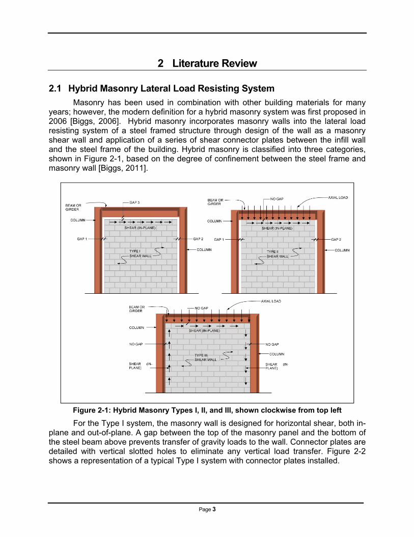
Masonry has been used in combination with other building materials for many years; however, the modern definition for a hybrid masonry system was first proposed in 2006 [Biggs, 2006]. Hybrid masonry incorporates masonry walls into the lateral load resisting system of a steel framed structure through design of the wall as a masonry shear wall and application of a series of shear connector plates between the infill wall and the steel frame of the building. Hybrid masonry is classified into three categories, shown in Figure 2-1, based on the degree of confinement between the steel frame and masonry wall [Biggs, 2011].

Figure 2-1: Hybrid Masonry Types I, II, and III, shown clockwise from top left

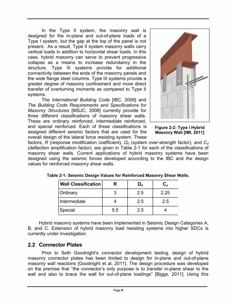
For the Type I system, the masonry wall is designed for horizontal shear, both in-plane and out-of-plane. A gap between the top of the masonry panel and the bottom of the steel beam above prevents transfer of gravity loads to the wall. Connector plates are detailed with vertical slotted holes to eliminate any vertical load transfer. Figure 2-2 shows a representation of a typical Type I system with connector plates installed.

Page 4

In the Type II system, the masonry wall is designed for the in-plane and out-of-plane loads of a Type I system, but the gap at the top of the panel is not present. As a result, Type II system masonry walls carry vertical loads in addition to horizontal shear loads. In this case, hybrid masonry can serve to prevent progressive collapse as a means to increase redundancy in the structure. Type III systems provide for additional connectivity between the ends of the masonry panels and the wide flange steel columns. Type III systems provide a greater degree of masonry confinement and more direct transfer of overturning moments as compared to Type II systems.

The International Building Code [IBC, 2006] and The Building Code Requirements and Specifications for Masonry Structures [MSJC, 2008] currently provide for three different classifications of masonry shear walls. These are ordinary reinforced, intermediate reinforced, and special reinforced. Each of these classifications is assigned different seismic factors that are used for the overall design of the lateral force resisting system. These factors, R (response modification coefficient), Ω0 (system over-strength factor), and Cd (deflection amplification factor), are given in Table 2-1 for each of the classifications of masonry shear walls. Current applications of hybrid masonry systems have been designed using the seismic forces developed according to the IBC and the design values for reinforced masonry shear walls.

Table 2-1: Seismic Design Values for Reinforced Masonry Shear Walls.

Hybrid masonry systems have been implemented in Seismic Design Categories A, B, and C. Extension of hybrid masonry load resisting systems into higher SDCs is currently under investigation. 2.2 Connector Plates

Prior to Seth Goodnight’s connector development testing, design of hybrid masonry connector plates has been limited to design for in-plane and out-of-plane masonry wall reactions [Goodnight et al, 2011]. The design procedure was developed on the premise that “the connector’s only purpose is to transfer in-plane shear to the wall and also to brace the wall for out-of-plane loadings” [Biggs, 2011]. Using this

Wall Classification R Ω0 Cd

Ordinary 3 2.5 2.25

Intermediate 4 2.5 2.5

Special 5.5 2.5 4

Figure 2-2: Type I Hybrid Masonry Wall [IMI, 2011]

Page 5

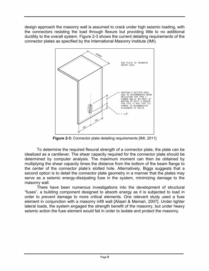
design approach the masonry wall is assumed to crack under high seismic loading, with the connectors resisting the load through flexure but providing little to no additional ductility to the overall system. Figure 2-3 shows the current detailing requirements of the connector plates as specified by the International Masonry Institute (IMI).

Figure 2-3: Connector plate detailing requirements [IMI, 2011]

To determine the required flexural strength of a connector plate, the plate can be

idealized as a cantilever. The shear capacity required for the connector plate should be determined by computer analysis. The maximum moment can then be obtained by multiplying the shear capacity times the distance from the bottom of the beam flange to the center of the connector plate’s slotted hole. Alternatively, Biggs suggests that a second option is to detail the connector plate geometry in a manner that the plates may serve as a seismic energy-dissipating fuse in the system, minimizing damage to the masonry wall.

There have been numerous investigations into the development of structural “fuses”, a building component designed to absorb energy as it is subjected to load in order to prevent damage to more critical elements. One relevant study used a fuse element in conjunction with a masonry infill wall [Aliaari & Memari, 2007]. Under lighter lateral loads, the system engaged the strength benefit of the masonry, but under heavy seismic action the fuse element would fail in order to isolate and protect the masonry.

Page 6

2.3 UHM Research

2.3.1 Connector Plates

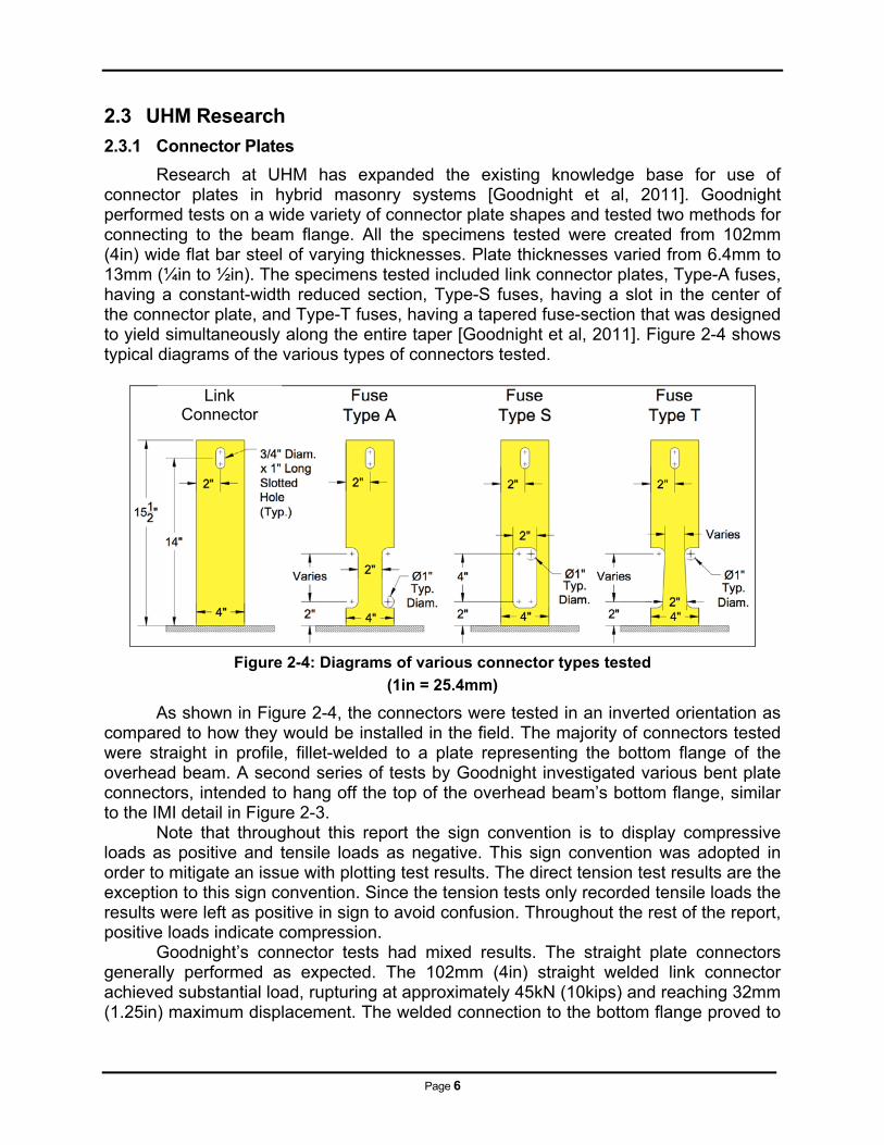
Research at UHM has expanded the existing knowledge base for use of connector plates in hybrid masonry systems [Goodnight et al, 2011]. Goodnight performed tests on a wide variety of connector plate shapes and tested two methods for connecting to the beam flange. All the specimens tested were created from 102mm (4in) wide flat bar steel of varying thicknesses. Plate thicknesses varied from 6.4mm to 13mm (¼in to ½in). The specimens tested included link connector plates, Type-A fuses, having a constant-width reduced section, Type-S fuses, having a slot in the center of the connector plate, and Type-T fuses, having a tapered fuse-section that was designed to yield simultaneously along the entire taper [Goodnight et al, 2011]. Figure 2-4 shows typical diagrams of the various types of connectors tested.

Figure 2-4: Diagrams of various connector types tested

(1in = 25.4mm)

As shown in Figure 2-4, the connectors were tested in an inverted orientation as compared to how they would be installed in the field. The majority of connectors tested were straight in profile, fillet-welded to a plate representing the bottom flange of the overhead beam. A second series of tests by Goodnight investigated various bent plate connectors, intended to hang off the top of the overhead beam’s bottom flange, similar to the IMI detail in Figure 2-3. Note that throughout this report the sign convention is to display compressive loads as positive and tensile loads as negative. This sign convention was adopted in order to mitigate an issue with plotting test results. The direct tension test results are the exception to this sign convention. Since the tension tests only recorded tensile loads the results were left as positive in sign to avoid confusion. Throughout the rest of the report, positive loads indicate compression. Goodnight’s connector tests had mixed results. The straight plate connectors generally performed as expected. The 102mm (4in) straight welded link connector achieved substantial load, rupturing at approximately 45kN (10kips) and reaching 32mm (1.25in) maximum displacement. The welded connection to the bottom flange proved to

Link Connector

Page 7

be the weak point for this connector. Interestingly, the Type-S fuse behaved somewhat similar to the link connector up until about 27kN (6kips) of load at which point the specimen began to buckle out-of-plane. It was observed from a series of varying aspect ratio Type-A fuses that a larger aspect ratio of fuse length to width generally provided a more ductile response. Additionally, testing a wide variety of connector thickness resulted in the conclusion that, for 102mm-wide connectors, using connectors thinner than 13mm was impractical as it typically resulted in undesirable out-of-plane buckling. The Type-T fuses were the most promising of all the connector types tested, showing superior energy dissipation capability and excellent displacement capacity. Unfortunately, the bent-plate connector tests proved largely unsuccessful due to premature failure of the flange-weld, caused by prying action [Goodnight et al, 2011]. The results from Goodnight’s tests guided the continued research at UHM in the proper direction. From the link connector tests, it was observed that a stronger, easier-to-install connection to the steel framing was required. The fuse tests demonstrated the viability of tapered fuses, but since the tapered fuses tested only reached approximately 13kN (3kips) at maximum load it was apparent that the nominal width of the fuses needed to be increased to achieve higher connector strengths. The bent plate tests showed that welding only at the beam flange was insufficient to restrain bent plate connectors. These observations were critical to the design of the next series of connector tests.

2.3.2 Bolt Push Out Tests

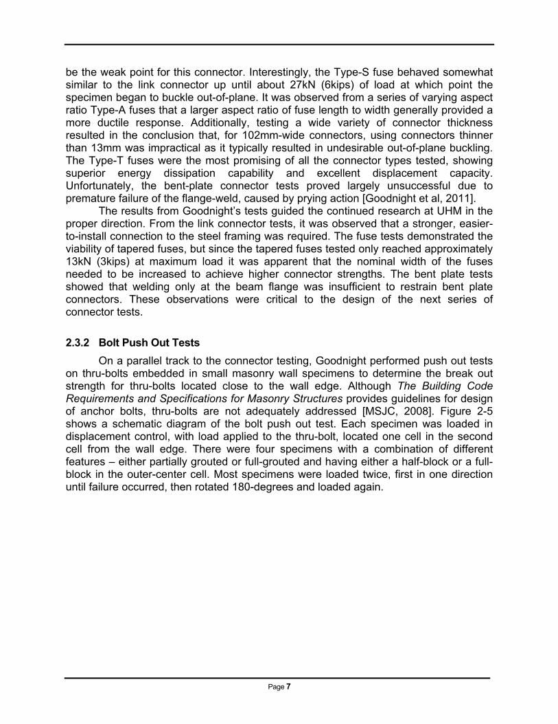
On a parallel track to the connector testing, Goodnight performed push out tests on thru-bolts embedded in small masonry wall specimens to determine the break out strength for thru-bolts located close to the wall edge. Although The Building Code Requirements and Specifications for Masonry Structures provides guidelines for design of anchor bolts, thru-bolts are not adequately addressed [MSJC, 2008]. Figure 2-5 shows a schematic diagram of the bolt push out test. Each specimen was loaded in displacement control, with load applied to the thru-bolt, located one cell in the second cell from the wall edge. There were four specimens with a combination of different features – either partially grouted or full-grouted and having either a half-block or a full-block in the outer-center cell. Most specimens were loaded twice, first in one direction until failure occurred, then rotated 180-degrees and loaded again.

Page 8

Figure 2-5: Bolt push out test schematic

(1in = 25.4mm)

The majority of specimens experienced masonry breakout failure at or above 89kN (20kips). For a pair of fuse connectors, it is important to remain below this strength value so that the fuses could act as the ductile elements in the system. Another lesson learned from the push out tests was that thru-bolts could not be made from standard 19mm (¾in) A307 threaded rod since the thru bolts made from this rod experienced shear failure at approximately the same load or even before the masonry breakout failure occurred. Thru-bolt location was also an issue – for the full-scale tests, it was deemed prudent to place the thru-bolts in the third cell from the edge of the walls to protect against potential breakout failure [Goodnight et al, 2011].

Page 9

3 Material Properties

3.1 Tension Tests

3.1.1 Motivation

Direct tension tests were performed in order to obtain accurate values for the material properties of the particular stock of ASTM grade A36 steel used for the connector tests. A36 steel has a required minimum yield strength of 248MPa (36ksi), but the actual strength of the material can often be significantly higher. Likewise the ultimate strength of A36 steel is required to be at least 400MPa (58ksi), but may be higher. To clearly define the connector steel’s stress-strain behavior, tension tests were performed according to ASTM E8 [ASTM, 2008].

3.1.2 Experimental Setup

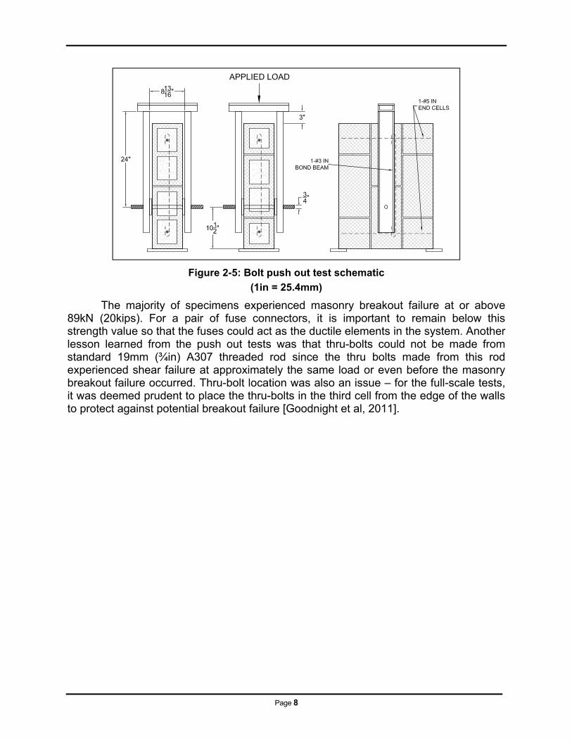
The tension tests were performed using an 810 MTS universal testing machine. An aluminum extensometer frame was designed and fabricated such that the extension could be measured on either side of the specimen. Averaging the measurements from both extensometers yielded the actual extension value. Figure 3-1 shows a photo of a specimen in the extensometer frame just prior to loading.

3.1.3 Test Specimens

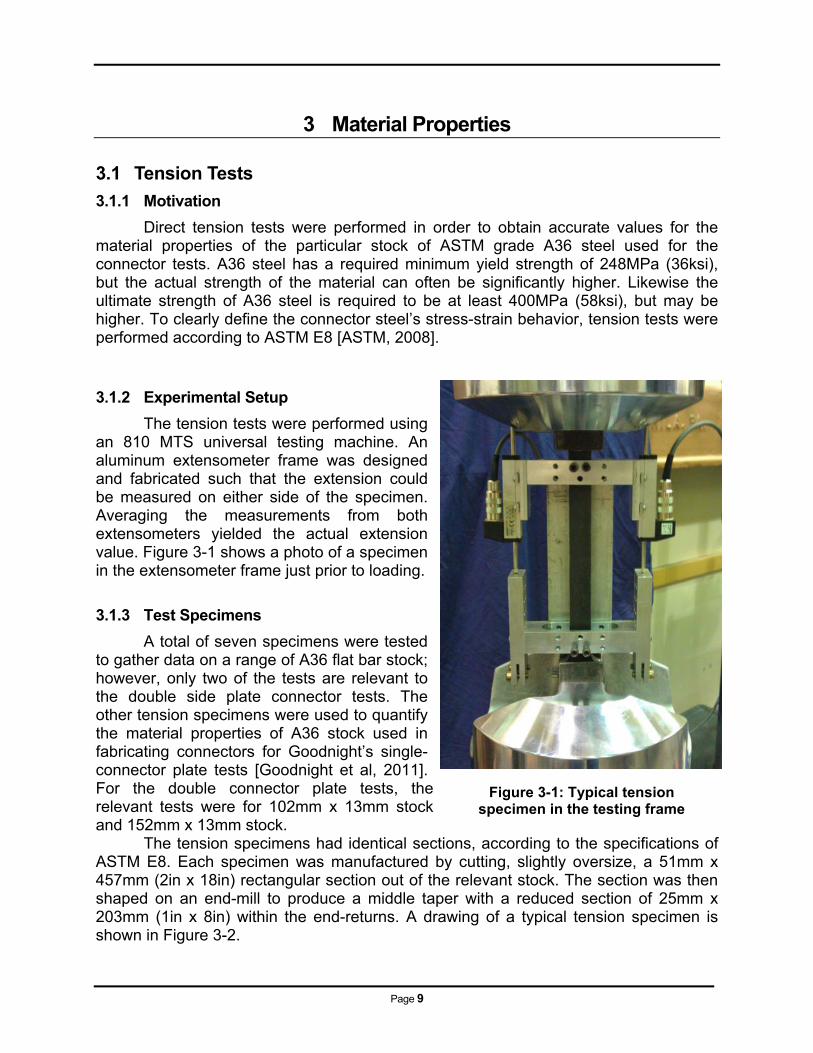
A total of seven specimens were tested to gather data on a range of A36 flat bar stock; however, only two of the tests are relevant to the double side plate connector tests. The other tension specimens were used to quantify the material properties of A36 stock used in fabricating connectors for Goodnight’s single-connector plate tests [Goodnight et al, 2011]. For the double connector plate tests, the relevant tests were for 102mm x 13mm stock and 152mm x 13mm stock. The tension specimens had identical sections, according to the specifications of ASTM E8. Each specimen was manufactured by cutting, slightly oversize, a 51mm x 457mm (2in x 18in) rectangular section out of the relevant stock. The section was then shaped on an end-mill to produce a middle taper with a reduced section of 25mm x 203mm (1in x 8in) within the end-returns. A drawing of a typical tension specimen is shown in Figure 3-2.

Figure 3-1: Typical tension specimen in the testing frame

Page 10

3.1.4 Test Procedure

Prior to testing, the dimensional properties of the reduced section for each specimen were recorded. Width and thickness were measured with calipers at three points along the 203mm gage length to obtain the average widths and thickness with fairly high precision. The specimen was then secured in the extensometer frame and loaded into the grips of the MTS test machine. Each specimen was tested using a displacement-control approach. Two different loading rates were used: first, a slow strain rate of 1.0με/sec (or 13mm/min, given the 203mm gauge length) in order to capture enough data points to develop the stress-strain curve. Once the specimen had yielded the test was paused and the loading rate was increased to 3.3με/sec (40.6mm/min), which was the same strain rate used for the connector tests. After the specimen failed, the total elongation of the specimen was measured by piecing the two halves of the specimen back together and re-measuring the original 203mm gage length.

3.2 Tension Test Results

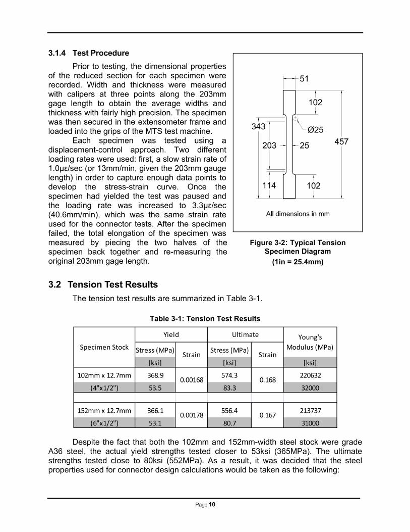
The tension test results are summarized in Table 3-1.

Table 3-1: Tension Test Results

Despite the fact that both the 102mm and 152mm-width steel stock were grade A36 steel, the actual yield strengths tested closer to 53ksi (365MPa). The ultimate strengths tested close to 80ksi (552MPa). As a result, it was decided that the steel properties used for connector design calculations would be taken as the following:

Stress (MPa) Stress (MPa)

[ksi] [ksi] [ksi]

102mm x 12.7mm 368.9 574.3 220632

(4"x1/2") 53.5 83.3 32000

152mm x 12.7mm 366.1 556.4 213737

(6"x1/2") 53.1 80.7 31000

Young's

Modulus (MPa)

UltimateYield

0.00178

0.00168

Strain Strain

0.168

0.167

Specimen Stock

Figure 3-2: Typical Tension Specimen Diagram

(1in = 25.4mm)

Page 11

Yield Strength = 50ksi (345MPa) Ultimate Strength = 80ksi (552MPa) Young’s Modulus = 30,000ksi (207GPa)

Poisson’s ratio for the steel was assumed to be 0.3. The relationship between Poisson’s ratio (ν), Young’s Modulus (E), and the Shear Modulus (G) is given by Equation 0:

………...... [Eqn 0]

Using Equation 0, the Shear Modulus was determined to be 11,540ksi (80GPa).

The full stress-strain curves for each tension specimen can be found in Appendix A2.

Page 12

Page 13

4 Approach

4.1 Double Side Plate Connector Testing

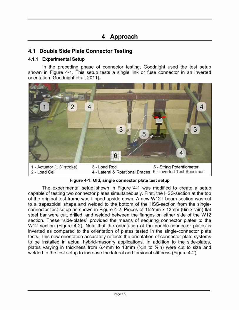
4.1.1 Experimental Setup

In the preceding phase of connector testing, Goodnight used the test setup shown in Figure 4-1. This setup tests a single link or fuse connector in an inverted orientation [Goodnight et al, 2011].

Figure 4-1: Old, single connector plate test setup

The experimental setup shown in Figure 4-1 was modified to create a setup capable of testing two connector plates simultaneously. First, the HSS-section at the top of the original test frame was flipped upside-down. A new W12 I-beam section was cut to a trapezoidal shape and welded to the bottom of the HSS-section from the single-connector test setup as shown in Figure 4-2. Pieces of 152mm x 13mm (6in x ½in) flat steel bar were cut, drilled, and welded between the flanges on either side of the W12 section. These “side-plates” provided the means of securing connector plates to the W12 section (Figure 4-2). Note that the orientation of the double-connector plates is inverted as compared to the orientation of plates tested in the single-connector plate tests. This new orientation accurately reflects the orientation of connector plate systems to be installed in actual hybrid-masonry applications. In addition to the side-plates, plates varying in thickness from 6.4mm to 13mm (¼in to ½in) were cut to size and welded to the test setup to increase the lateral and torsional stiffness (Figure 4-2).

6

6 - Inverted Test Specimen

Page 14

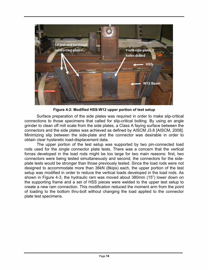
Figure 4-2: Modified HSS-W12 upper portion of test setup

Surface preparation of the side plates was required in order to make slip-critical connections to those specimens that called for slip-critical bolting. By using an angle grinder to clean off mill scale from the side plates, a Class A faying surface between the connectors and the side plates was achieved as defined by AISCM J3.8 [AISCM, 2008]. Minimizing slip between the side-plate and the connector was desirable in order to obtain clear hysteretic load-displacement data.

The upper portion of the test setup was supported by two pin-connected load rods used for the single connector plate tests. There was a concern that the vertical forces developed in the load rods might be too large for two main reasons: first, two connectors were being tested simultaneously and second, the connectors for the side-plate tests would be stronger than those previously tested. Since the load rods were not designed to accommodate more than 36kN (8kips) each, the upper portion of the test setup was modified in order to reduce the vertical loads developed in the load rods. As shown in Figure 4-3, the hydraulic ram was moved about 380mm (15”) lower down on the supporting frame and a set of HSS pieces were welded to the upper test setup to create a new ram connection. This modification reduced the moment arm from the point of loading to the bottom thru-bolt without changing the load applied to the connector plate test specimens.

W12 Beam

HSS

Page 15

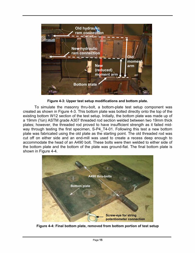
Figure 4-3: Upper test setup modifications and bottom plate.

To simulate the masonry thru-bolt, a bottom-plate test setup component was created as shown in Figure 4-3. This bottom plate was bolted directly onto the top of the existing bottom W12 section of the test setup. Initially, the bottom plate was made up of a 19mm (¾in) ASTM grade A307 threaded rod section welded between two 19mm thick plates; however, the threaded rod proved to have insufficient strength as it failed mid-way through testing the first specimen, S-P4_T4-01. Following this test a new bottom plate was fabricated using the old plate as the starting point. The old threaded rod was cut off on either side and an end-mill was used to create a recess deep enough to accommodate the head of an A490 bolt. These bolts were then welded to either side of the bottom plate and the bottom of the plate was ground-flat. The final bottom plate is shown in Figure 4-4.

Figure 4-4: Final bottom plate, removed from bottom portion of test setup

Old hydraulic ram connection

New hydraulic ram connection

New (reduced) moment arm

Old moment arm

Bottom plate

Bottom plate

A490 thru-bolts

Screw-eye for string potentiometer connection

Page 16

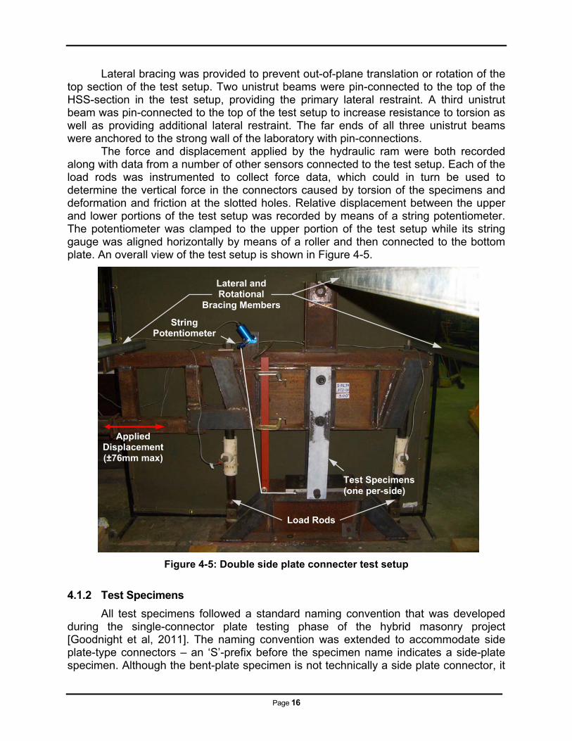
Lateral bracing was provided to prevent out-of-plane translation or rotation of the top section of the test setup. Two unistrut beams were pin-connected to the top of the HSS-section in the test setup, providing the primary lateral restraint. A third unistrut beam was pin-connected to the top of the test setup to increase resistance to torsion as well as providing additional lateral restraint. The far ends of all three unistrut beams were anchored to the strong wall of the laboratory with pin-connections.

The force and displacement applied by the hydraulic ram were both recorded along with data from a number of other sensors connected to the test setup. Each of the load rods was instrumented to collect force data, which could in turn be used to determine the vertical force in the connectors caused by torsion of the specimens and deformation and friction at the slotted holes. Relative displacement between the upper and lower portions of the test setup was recorded by means of a string potentiometer. The potentiometer was clamped to the upper portion of the test setup while its string gauge was aligned horizontally by means of a roller and then connected to the bottom plate. An overall view of the test setup is shown in Figure 4-5.

Figure 4-5: Double side plate connecter test setup

4.1.2 Test Specimens

All test specimens followed a standard naming convention that was developed during the single-connector plate testing phase of the hybrid masonry project [Goodnight et al, 2011]. The naming convention was extended to accommodate side plate-type connectors – an ‘S’-prefix before the specimen name indicates a side-plate specimen. Although the bent-plate specimen is not technically a side plate connector, it

Load Rods

Test Specimens (one per-side)

Applied Displacement (±76mm max)

String Potentiometer

Lateral and Rotational

Bracing Members

Page 17

still received the S-prefix because the test setup configuration was essentially the same as for the side-plate tests. Each specimen’s side plate connection method falls under the miscellaneous section of the specimen name, just after the fuse-type designation. For the welded specimen, the suffix ‘W’ is used, while the bent plate specimen used the suffix ‘BP.’ All other connections were bolted with two to four A490 bolts. The naming convention is documented in Table 4-1, which shows the names developed for the six double connector specimens tested in this program. Note that all specimen names are developed using US Customary units.

Table 4-1: Connector Naming Convention Summary

Note: Fuses of type ‘T’ are tapered fuses and the associated number is the aspect ratio of the

fuse, based on fuse length divided by the widest fuse dimension. ‘W’ indicates welded connection; ‘BP’ indicates bent plate and welded; all others are bolted.

For this series of tests a total of six different specimens were examined as listed

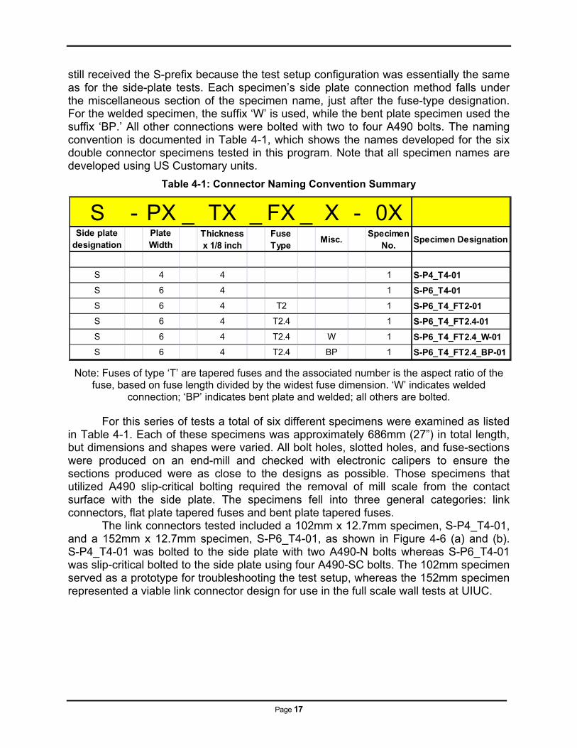
in Table 4-1. Each of these specimens was approximately 686mm (27”) in total length, but dimensions and shapes were varied. All bolt holes, slotted holes, and fuse-sections were produced on an end-mill and checked with electronic calipers to ensure the sections produced were as close to the designs as possible. Those specimens that utilized A490 slip-critical bolting required the removal of mill scale from the contact surface with the side plate. The specimens fell into three general categories: link connectors, flat plate tapered fuses and bent plate tapered fuses. The link connectors tested included a 102mm x 12.7mm specimen, S-P4_T4-01, and a 152mm x 12.7mm specimen, S-P6_T4-01, as shown in Figure 4-6 (a) and (b). S-P4_T4-01 was bolted to the side plate with two A490-N bolts whereas S-P6_T4-01 was slip-critical bolted to the side plate using four A490-SC bolts. The 102mm specimen served as a prototype for troubleshooting the test setup, whereas the 152mm specimen represented a viable link connector design for use in the full scale wall tests at UIUC.

S - PX _ TX _ FX _ X - 0XSide plate

designationPlate Width

Thickness x 1/8 inch

Fuse Type

Misc.Specimen

No.Specimen Designation

S 4 4 1 S-P4_T4-01

S 6 4 1 S-P6_T4-01

S 6 4 T2 1 S-P6_T4_FT2-01

S 6 4 T2.4 1 S-P6_T4_FT2.4-01

S 6 4 T2.4 W 1 S-P6_T4_FT2.4_W-01

S 6 4 T2.4 BP 1 S-P6_T4_FT2.4_BP-01

Page 18

Figure 4-6: Link Connector Specimens: (a) S-P4_T4-01; (b) S-P6_T4-01

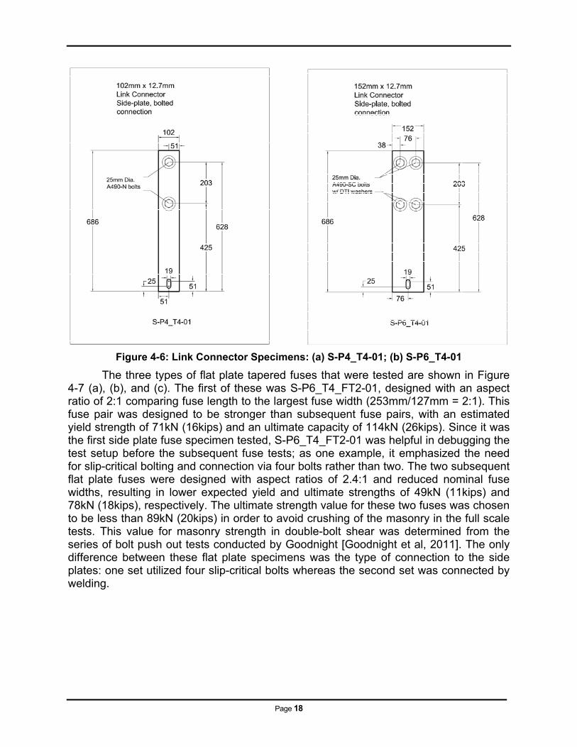
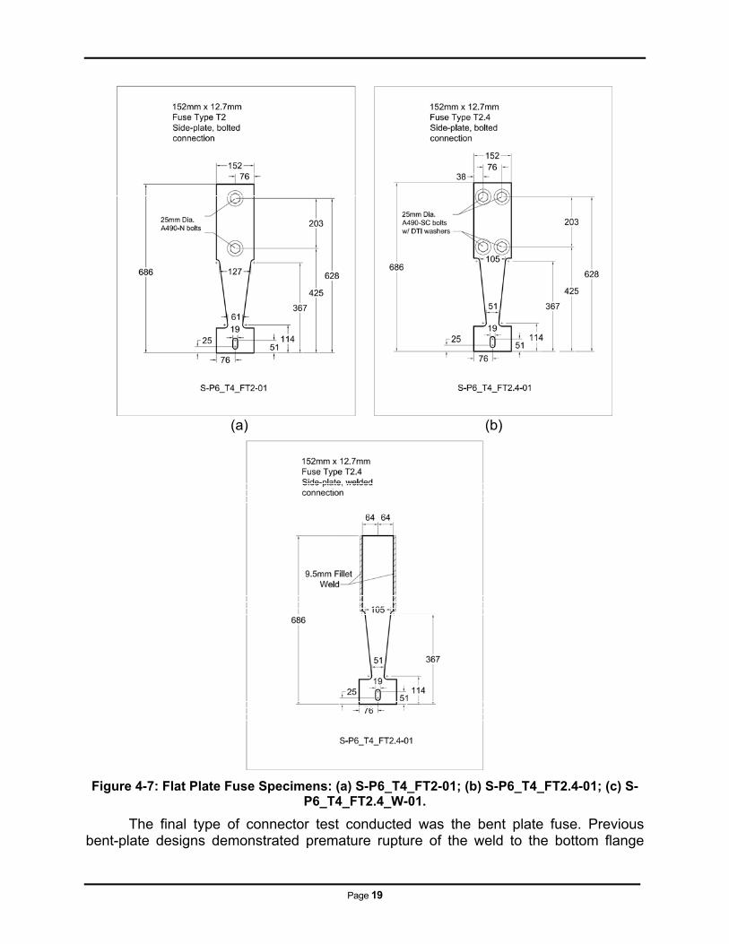
The three types of flat plate tapered fuses that were tested are shown in Figure 4-7 (a), (b), and (c). The first of these was S-P6_T4_FT2-01, designed with an aspect ratio of 2:1 comparing fuse length to the largest fuse width (253mm/127mm = 2:1). This fuse pair was designed to be stronger than subsequent fuse pairs, with an estimated yield strength of 71kN (16kips) and an ultimate capacity of 114kN (26kips). Since it was the first side plate fuse specimen tested, S-P6_T4_FT2-01 was helpful in debugging the test setup before the subsequent fuse tests; as one example, it emphasized the need for slip-critical bolting and connection via four bolts rather than two. The two subsequent flat plate fuses were designed with aspect ratios of 2.4:1 and reduced nominal fuse widths, resulting in lower expected yield and ultimate strengths of 49kN (11kips) and 78kN (18kips), respectively. The ultimate strength value for these two fuses was chosen to be less than 89kN (20kips) in order to avoid crushing of the masonry in the full scale tests. This value for masonry strength in double-bolt shear was determined from the series of bolt push out tests conducted by Goodnight [Goodnight et al, 2011]. The only difference between these flat plate specimens was the type of connection to the side plates: one set utilized four slip-critical bolts whereas the second set was connected by welding.

Page 19

(a) (b)

Figure 4-7: Flat Plate Fuse Specimens: (a) S-P6_T4_FT2-01; (b) S-P6_T4_FT2.4-01; (c) S-P6_T4_FT2.4_W-01.

The final type of connector test conducted was the bent plate fuse. Previous bent-plate designs demonstrated premature rupture of the weld to the bottom flange

Page 20

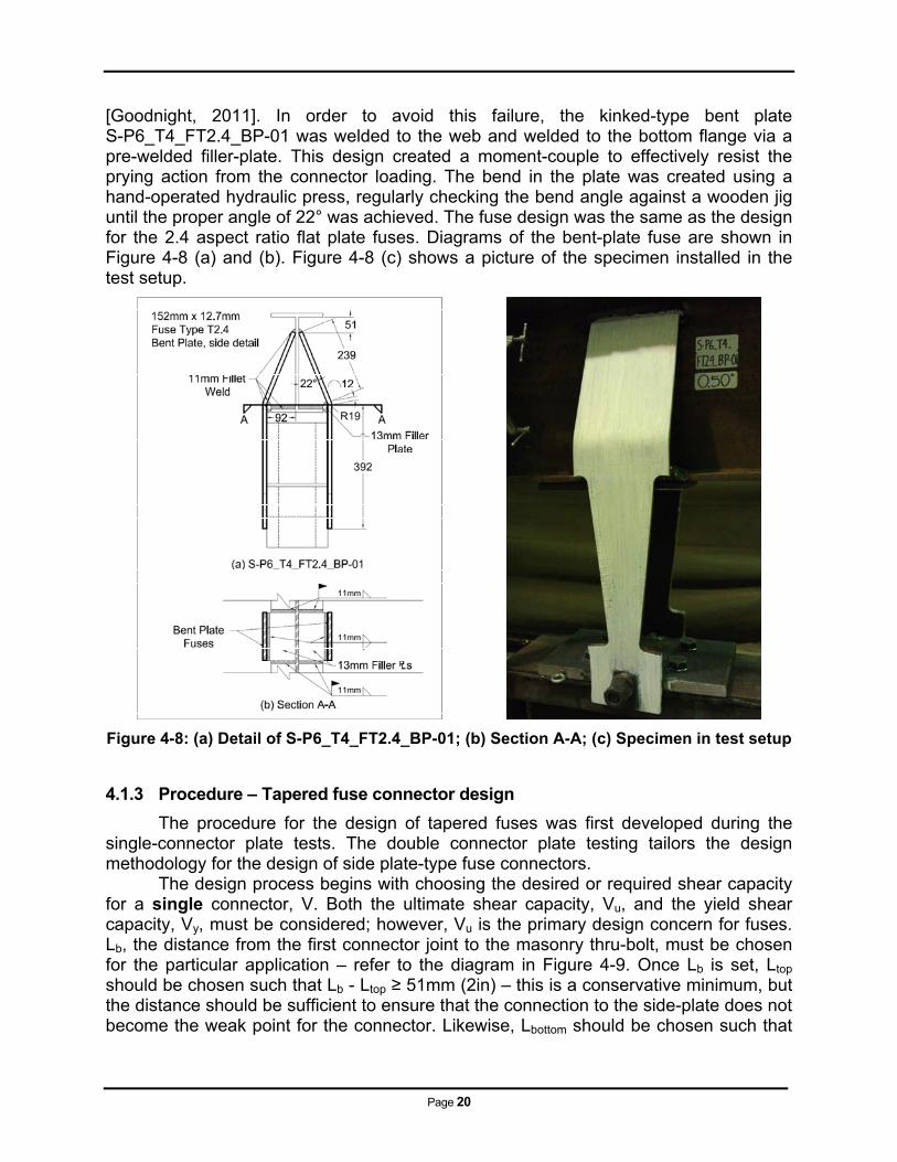
[Goodnight, 2011]. In order to avoid this failure, the kinked-type bent plate S-P6_T4_FT2.4_BP-01 was welded to the web and welded to the bottom flange via a pre-welded filler-plate. This design created a moment-couple to effectively resist the prying action from the connector loading. The bend in the plate was created using a hand-operated hydraulic press, regularly checking the bend angle against a wooden jig until the proper angle of 22° was achieved. The fuse design was the same as the design for the 2.4 aspect ratio flat plate fuses. Diagrams of the bent-plate fuse are shown in Figure 4-8 (a) and (b). Figure 4-8 (c) shows a picture of the specimen installed in the test setup.

Figure 4-8: (a) Detail of S-P6_T4_FT2.4_BP-01; (b) Section A-A; (c) Specimen in test setup

4.1.3 Procedure – Tapered fuse connector design

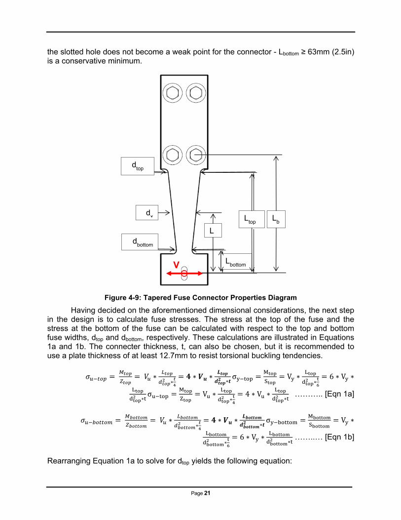
The procedure for the design of tapered fuses was first developed during the single-connector plate tests. The double connector plate testing tailors the design methodology for the design of side plate-type fuse connectors. The design process begins with choosing the desired or required shear capacity for a single connector, V. Both the ultimate shear capacity, Vu, and the yield shear capacity, Vy, must be considered; however, Vu is the primary design concern for fuses. Lb, the distance from the first connector joint to the masonry thru-bolt, must be chosen for the particular application – refer to the diagram in Figure 4-9. Once Lb is set, Ltop should be chosen such that Lb - Ltop ≥ 51mm (2in) – this is a conservative minimum, but the distance should be sufficient to ensure that the connection to the side-plate does not become the weak point for the connector. Likewise, Lbottom should be chosen such that

Page 21

the slotted hole does not become a weak point for the connector - Lbottom ≥ 63mm (2.5in) is a conservative minimum.

Figure 4-9: Tapered Fuse Connector Properties Diagram

Having decided on the aforementioned dimensional considerations, the next step in the design is to calculate fuse stresses. The stress at the top of the fuse and the stress at the bottom of the fuse can be calculated with respect to the top and bottom fuse widths, dtop and dbottom, respectively. These calculations are illustrated in Equations 1a and 1b. The connecter thickness, t, can also be chosen, but it is recommended to use a plate thickness of at least 12.7mm to resist torsional buckling tendencies.

σM

SV

L6 V

Lσ

M

ZV

L4 V

L ……….. [Eqn 1a]

σ M

SV

L 6 V L ……..… [Eqn 1b]

Rearranging Equation 1a to solve for dtop yields the following equation:

Lb L

top

Lbottom

dbottom

dtop

dx

L

V

Page 22

4 ……..… [Eqn 2a]

(Note: Equation 2b could also be derived, but it is not necessary to do so) Using Equation 2a, dtop can be determined by using the ultimate strength of the connecter steel (552MPa, 80kips) for σu-top. dbottom could be determined in a similar manner, but another method is to set [Eqn 1a] = [Eqn 1b] and simplify. The goal for tapered fuses is for yielding to occur simultaneously along the entire fuse length, thus σy-top = σy-bottom and σu-top = σu-bottom. Although Equation 1 shows that there is a quadratic

relationship between stress and fuse width ( 4 ), the variation of stress

over the fuse length is close enough to linear that fuse yielding should occur nearly simultaneously along the fuse length. Setting the stress at the top of the fuse equal to the stress at the bottom of the fuse and simplifying, the following relation can be derived:

……..… [Eqn 3]

Substituting dtop in Equation 3 results in the remaining width, dbottom. This concludes the design for the ultimate shear, but the yield shear capacity should still be considered. The equations are similar to the ultimate shear design equations, the primary difference being the use of the elastic section, S = d2*t/6, instead of the plastic modulus, Z = d2*t/4. Substituting this relation into Equation 1a and rearranging to solve for yield shear force, Vy, gives the following:

6 2

……..… [Eqn 4]

The yield force is obtained by substituting the yield shear strength (345MPa, 50kips) for σy-top in Equation 4. Note that yield force could be calculated at the bottom of the fuse instead of the top, but the result would be the same. Although the yield force is not a critical value for fuse connectors it is still a worthwhile consideration in designing tapered fuses. Fuse connectors should remain below the yield load for wind and low seismic loads. In addition to designing the fuse there are several other design checks that are necessary for side-plate connectors. Consideration was already given to avoid bearing or tear-out type failures near the slotted hole and near the bottom side-plate connection, thus these two failure modes should not be factors. The primary failure mode that should be considered for a side-plate connector is failure of the plate due to lateral torsional buckling. Additional failure modes concern the bolts and side-plates: shear failure of the bottom bolt, shear failure of the bottom row of side-plate bolts (or of the weld-group if a welded connection to the side-plate is used), and shear failure of the welds securing the side-plate to the flanges of the top I-beam. Because the connector plate is under a complex state of stress, it is difficult to estimate failure due to lateral torsional buckling. This is complicated by the fact that the connector plates weaken with metal fatigue. This failure mode for the connecter plates has not been fully addressed in the design of the specimens. As the hybrid masonry

Page 23

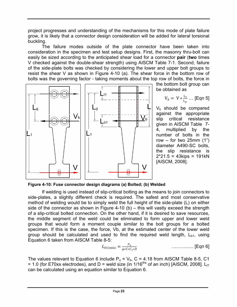
project progresses and understanding of the mechanisms for this mode of plate failure grow, it is likely that a connector design consideration will be added for lateral torsional buckling. The failure modes outside of the plate connector have been taken into consideration in the specimen and test setup designs. First, the masonry thru-bolt can easily be sized according to the anticipated shear load for a connector pair (two times V checked against the double-shear strength) using AISCM Table 7-1. Second, failure of the side-plate bolts was checked by considering the lower and upper bolt groups to resist the shear V as shown in Figure 4-10 (a). The shear force in the bottom row of bolts was the governing factor - taking moments about the top row of bolts, the force in

the bottom bolt group can be obtained as

V V L1

L … [Eqn 5]

Vb should be compared against the appropriate slip critical resistance given in AISCM Table 7-4, multiplied by the number of bolts in the row – for two 25mm (1”) diameter A490-SC bolts, the slip resistance is 2*21.5 = 43kips = 191kN [AISCM, 2008].

Figure 4-10: Fuse connector design diagrams (a) Bolted; (b) Welded

If welding is used instead of slip-critical bolting as the means to join connectors to side-plates, a slightly different check is required. The safest and most conservative method of welding would be to simply weld the full height of the side-plate (L) on either side of the connector as shown in Figure 4-10 (b) – this will vastly exceed the strength of a slip-critical bolted connection. On the other hand, if it is desired to save resources, the middle segment of the weld could be eliminated to form upper and lower weld groups that would form a moment couple similar to the bolt groups for a bolted specimen. If this is the case, the force, Vb, at the estimated center of the lower weld group should be calculated and used to find the required weld length, Lb1, using Equation 6 taken from AISCM Table 8-5:

1 min1

………...... [Eqn 6]

The values relevant to Equation 6 include Pu = Vb, C = 4.18 from AISCM Table 8-5, C1 = 1.0 (for E70xx electrodes), and D = weld size (in 1/16ths of an inch) [AISCM, 2008]. Lt1 can be calculated using an equation similar to Equation 6.

Page 24

For the purpose of the test at the UHM, the goal was not to create the most efficient welded design, but rather to compare the results between slip-critical bolted and welded specimens having the same fuse section. As a result, the welded specimen was secured with 9.5mm (3/8”) fillet welds running the full-height of the side-plates on either side of the connectors and no further studies were performed into optimizing the weld design.

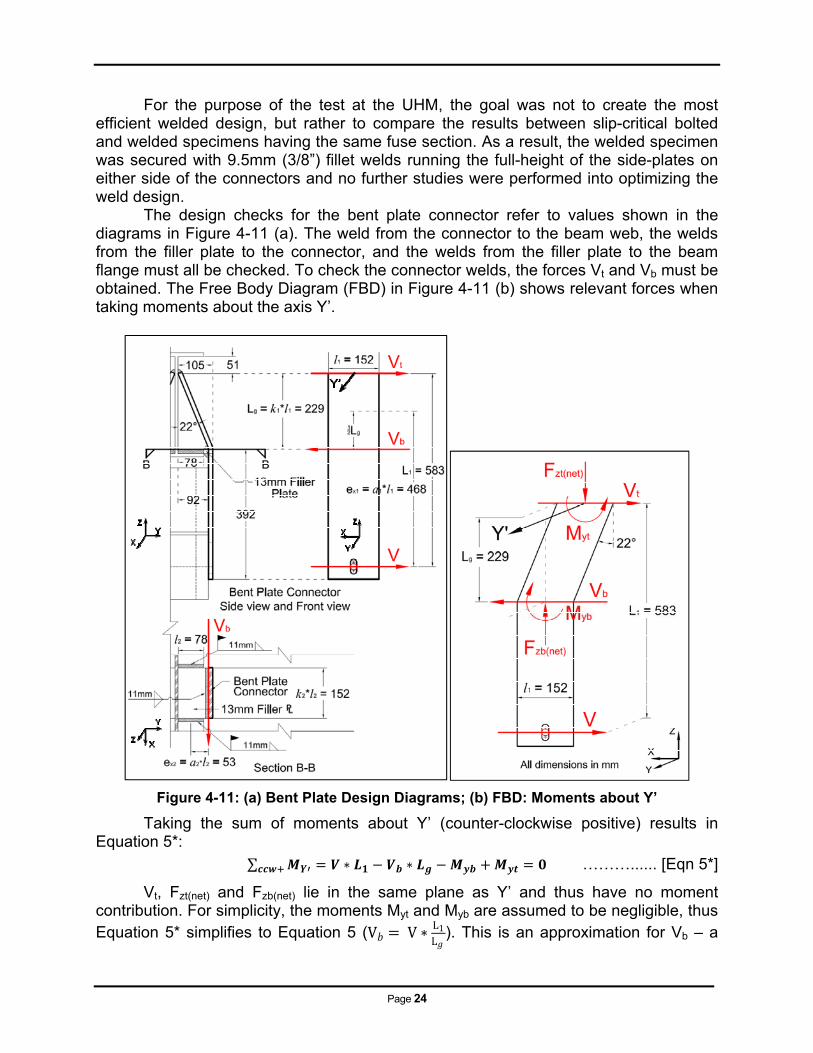
The design checks for the bent plate connector refer to values shown in the diagrams in Figure 4-11 (a). The weld from the connector to the beam web, the welds from the filler plate to the connector, and the welds from the filler plate to the beam flange must all be checked. To check the connector welds, the forces Vt and Vb must be obtained. The Free Body Diagram (FBD) in Figure 4-11 (b) shows relevant forces when taking moments about the axis Y’.

Figure 4-11: (a) Bent Plate Design Diagrams; (b) FBD: Moments about Y’

Taking the sum of moments about Y’ (counter-clockwise positive) results in Equation 5*:

∑ ………...... [Eqn 5*]

Vt, Fzt(net) and Fzb(net) lie in the same plane as Y’ and thus have no moment contribution. For simplicity, the moments Myt and Myb are assumed to be negligible, thus Equation 5* simplifies to Equation 5 (V V L1

L ). This is an approximation for Vb – a

Page 25

more accurate value could be obtained by using a structural analysis program such as SAP 2000.

Once Vb has been determined, Vt is easily calculated by considering equilibrium of forces in the X-direction. The adequacy of the weld between the beam web and the connector can be checked by comparing Vt against the strength of a the fillet weld given by :

………...... [Eqn 7]

where = 0.75 , Fw = 0.6*FEXX (FEXX = 70ksi for E70 Electrode), Aw = weld length (l)*groove depth (11mm maximum for a 13mm thick plate) [AISCM, 2008]. The adequacy of the weld between the filler plate and the connector can be checked by comparing the result from Equation 7 against Vb/2 (since there are two welds that share the burden of Vb).

Another check for the adequacy of the connector welds may be performed using AISCM Table 8-4. Using the relevant values ex1, a1, k1, and l1 from Figure 4-11 (a), Equation 6 can be rearranged and used to calculate the strength of the weld group, Pu1:

1 1 1 ………...... [Eqn 8]

where D is the weld size (in 1/16s of an inch), C = coefficient from AISCM Table 8-4, the electrode coefficient C1 = 1.0, and l1 = the length of each weld (152mm or 6in for this particular connector). If Pu1 is greater or equal to V then the weld group’s strength is adequate. A downside of this method is that it does not account for the two fillet welds that contribute to Vb. Additionally, the AISCM table method allows for calculation of the strength of the weld group but not the calculation of Vb and Vt individually [AISCM, 2008].

The adequacy of the welds between the filler plate and the beam flange can be checked using AISCM Table 8-5 and Equation 8 ( 2 1 2). Section B-B in Figure 4-11 (a) shows the relevant values for ex2, a2, k2, and l2 that can be used with AISCM Table 8-4 to obtain the coefficient C. The weld group’s strength, Pu2, should be greater than or equal to Vb. The final design consideration, securing the side-plates to the beam flanges, is a simple check. AISCM Table 8-4 can be used to design the two lines of weld for a parallel eccentric load [AISCM, 2008]. The governing equation for the design is Equation 8 ( 2 1 ), where l is the length of the welds between the side-plate and the flanges. For an 11mm (7/16in) weld, the largest possible for a 152mm (1/2in) thick plate, the available shear capacity of the weld group was 140kN (31kips) which was much larger than any anticipated shear load from a single connector.

4.1.4 Procedure – Theoretical Yield Points and Ultimate Load Calculations

In order to give a reasonable analysis of the experimental results, it was necessary to calculate the theoretical yield points and the theoretical ultimate load capacity for each specimen. The calculations for S-P6_T4-01 are shown here as an example. The calculations for all other specimens followed a similar procedure.

Page 26

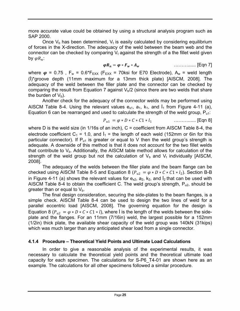
The first calculation performed was for the yield force. As shown in Figure 4-12 it was assumed that the specimen would yield at the reduced net section at the lower bolted connection to the side plate. Yielding would initiate due to a moment, My, applied by the force at the masonry thru-bolt, Vy

*. The moment arm, x, was taken to be the distance from the plastic hinge to the masonry thru-bolt, assuming the thru-bolt was at the top of the slotted hole. From the tension specimen tests, the connector steel’s yield strength, σy, was assumed to be 345MPa (50ksi). According to Euler-Bernoulli beam theory, the bending stress can be written as:

………...... [Eqn 9]

where y is the distance to the extreme fiber (76mm, 3in) and S and I are the section modulus and moment of inertia, respectively, at the section being considered.

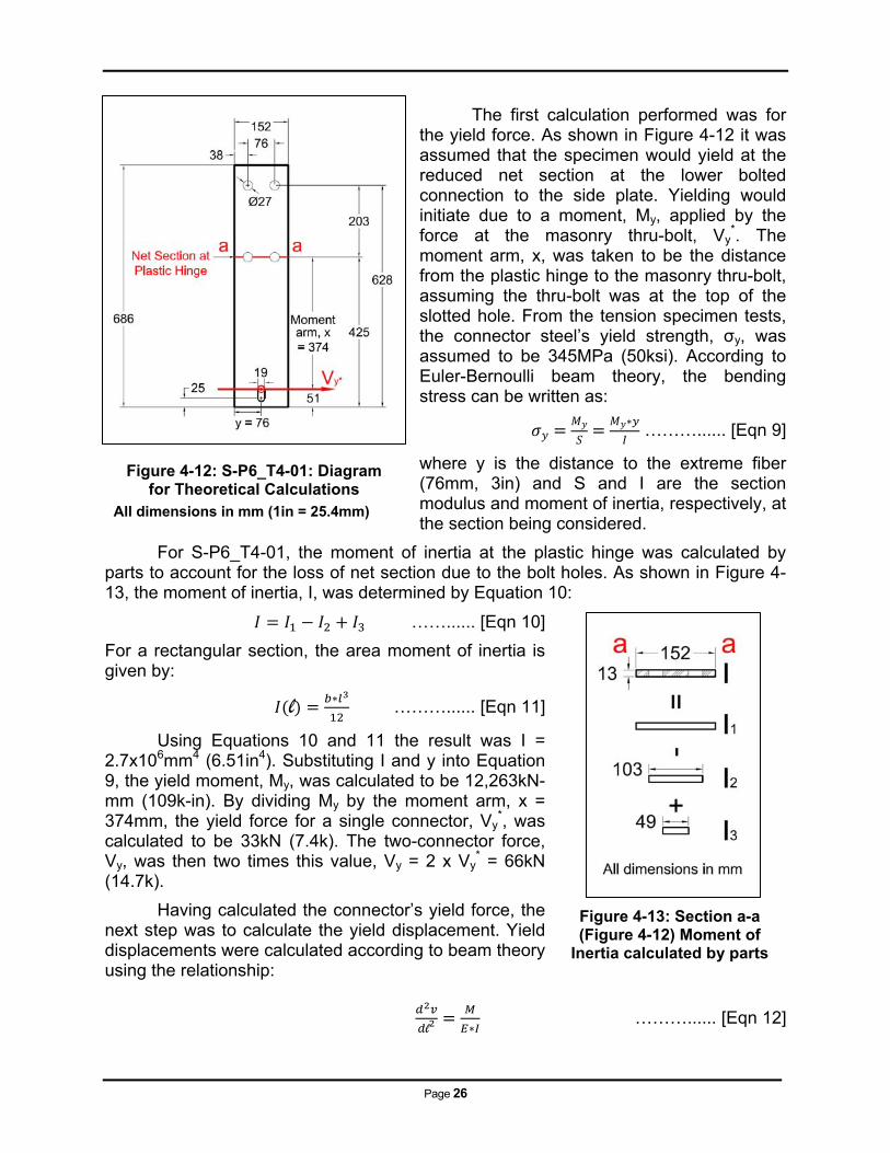
For S-P6_T4-01, the moment of inertia at the plastic hinge was calculated by parts to account for the loss of net section due to the bolt holes. As shown in Figure 4-13, the moment of inertia, I, was determined by Equation 10:

……...... [Eqn 10]

For a rectangular section, the area moment of inertia is given by:

l ………...... [Eqn 11]

Using Equations 10 and 11 the result was I = 2.7x106mm4 (6.51in4). Substituting I and y into Equation 9, the yield moment, My, was calculated to be 12,263kN-mm (109k-in). By dividing My by the moment arm, x = 374mm, the yield force for a single connector, Vy

*, was calculated to be 33kN (7.4k). The two-connector force, Vy, was then two times this value, Vy = 2 x Vy

* = 66kN (14.7k).

Having calculated the connector’s yield force, the next step was to calculate the yield displacement. Yield displacements were calculated according to beam theory using the relationship:

l ………...... [Eqn 12]

a a

Figure 4-12: S-P6_T4-01: Diagram for Theoretical Calculations

All dimensions in mm (1in = 25.4mm)

Figure 4-13: Section a-a (Figure 4-12) Moment of

Inertia calculated by parts

Page 27

where v = deflection due to bending, = curvature, M = bending moment, E =

modulus of elasticity, and I = moment of inertia about the neutral axis of the member. Using Equation 12 the deflection could be obtained by double-integration of the bending

moment equation and application of boundary conditions.

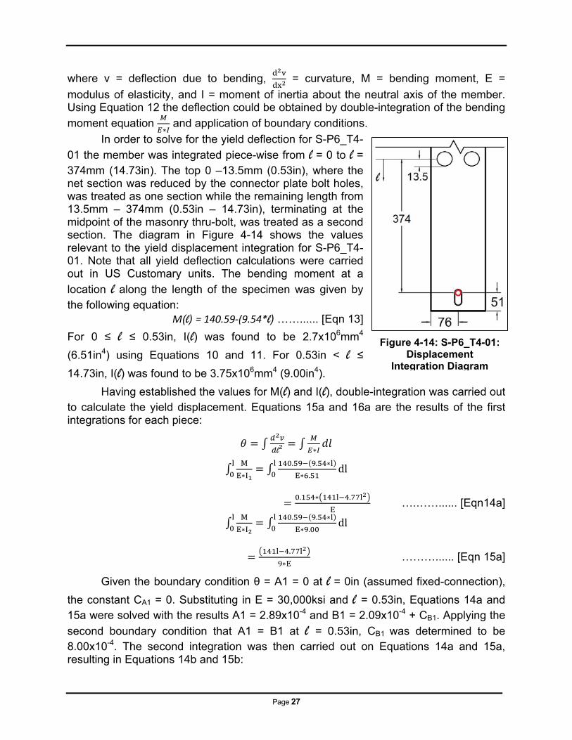
In order to solve for the yield deflection for S-P6_T4-

01 the member was integrated piece-wise from l = 0 to l = 374mm (14.73in). The top 0 –13.5mm (0.53in), where the net section was reduced by the connector plate bolt holes, was treated as one section while the remaining length from 13.5mm – 374mm (0.53in – 14.73in), terminating at the midpoint of the masonry thru-bolt, was treated as a second section. The diagram in Figure 4-14 shows the values relevant to the yield displacement integration for S-P6_T4-01. Note that all yield deflection calculations were carried out in US Customary units. The bending moment at a

location l along the length of the specimen was given by the following equation:

M(l) = 140.59‐(9.54*l) ……...... [Eqn 13]

For 0 ≤ l ≤ 0.53in, I(l) was found to be 2.7x106mm4

(6.51in4) using Equations 10 and 11. For 0.53in < l ≤

14.73in, I(l) was found to be 3.75x106mm4 (9.00in4).

Having established the values for M(l) and I(l), double-integration was carried out to calculate the yield displacement. Equations 15a and 16a are the results of the first integrations for each piece:

l

M

E I

. .

E .dl

. .

E ….……...... [Eqn14a]

M

E I

. .

E .dl

.

E ………...... [Eqn 15a]

Given the boundary condition θ = A1 = 0 at l = 0in (assumed fixed-connection),

the constant CA1 = 0. Substituting in E = 30,000ksi and l = 0.53in, Equations 14a and 15a were solved with the results A1 = 2.89x10-4 and B1 = 2.09x10-4 + CB1. Applying the

second boundary condition that A1 = B1 at l = 0.53in, CB1 was determined to be 8.00x10-4. The second integration was then carried out on Equations 14a and 15a, resulting in Equations 14b and 15b:

Figure 4-14: S-P6_T4-01: Displacement

Integration Diagram

Page 28

l

2. . .

2 5.12 10 54.2 1.23 ……...... [Eqn 14b]

2. .

8.00 10

2 8.00 10. .

………...... [Eqn 15b]

Given the boundary condition v = A2 = 0 at l = 0in (assumed fixed-connection),

the constant CA2 = 0. Checking the boundary at l = 0.53in, Equations 14b and 15b were solved with the results A2 = 7.71x10-5 and B2 = 9.82x10-5 + CB2. Applying the second

boundary condition that A2 = B2 at l = 0.53in, CB2 was determined to be -2.11x10-5. Rewriting Equation 15b:

0.53in < l ≤ 14.73in: 2 8.00 10 2.11 10. .

...… [Eqn 15b]

Using Equation 15b, the yield displacement due to the bending moment, ∆yM, at l = 14.73in was found to be = 0.030in (0.77mm).

To increase the accuracy of results, deflection caused by shear deformation (∆yS) was considered in addition to the bending deformation. The connector plates tested were all relatively wide compared to their unrestrained length which could potentially result in significant deflection contributions from shear. For example, S-P6_T4-01 had a length to width ratio of 425mm/152mm = 2.8:1. Equation 16a was used to solve for the deflection due to shear deformation:

………...... [Eqn 16a]

In Equation 16a, G is the shear modulus (80GPa, 11,500ksi), A is the effective shear area, and β is the form factor, a constant representing the state of stress through the width of the connector [Megson, 2005]. For rectangular sections β = 6/5. The link connectors are constant width rectangular sections which allow for Equation 16a to be simplified to Equation 16b:

………...... [Eqn 16b]

The shear deformation for S-P6_T4-01 was calculated in two parts using Equation 16b. Adding together the deflections over 0 –13.5mm and 13.5mm – 374mm, the total deflection caused by shear was determined as 0.0038in (0.1mm). The total deflection was then 0.034in (0.86mm).

The last theoretical calculation to be performed was for each connector’s ultimate load. Three different procedures were used to estimate ultimate loads. The first method results in a lower boundary estimate of the ultimate load by calculating the plastic moment as

Page 29

………...... [Eqn 17a]

where σy is the steel yield stress (345MPa, 50ksi) and Z represents the plastic section

modulus. for a rectangular section.

The second ultimate load estimation method provided an upper boundary for the load predictions. This method assumed that each connector yielded completely right up to the plastic neutral axis. The load predictions were obtained from Equation 17b.

………...... [Eqn 17b]

The final method of estimating the ultimate loads used the elastic section modulus / in conjunction with the ultimate steel stress, σu. This approach produced load estimates that were slightly higher than those resulting from Equation 17a. Equation 17c was used in this load prediction method.

………...... [Eqn 17c]

For S-P6_T4-01, the plastic section modulus, Z = 45,000mm3(2.75in3), was determined using a section properties calculation program. The ultimate moment was obtained three ways resulting in Mp = 137k-in, Mp* = 220k-in, and Mp** = 174k-in for Equation 17 (a), (b), and (c), respectively. From these moments was calculated from the equation . The ultimate force for two connectors was then calculated as Vu = 2 x Vu*. The resulting forces were 83kN (19kips), 133kN (30kips), and 105kN (24kips) from Mp, Mp*, and Mp**, respectively. Tables summarizing calculations for yield loads, yield displacements, and ultimate loads can be found in Appendices A3-A5. Note that all integrations for yield displacements were performed using the program WxMaxima.

4.1.5 Procedure – Double side plate connector testing

Testing began by starting up the MTS TestStar II controller and bringing the hydraulic ram up to full pressure before a specimen was installed in the test setup. This ensured that the specimen would not be damaged if the hydraulic ram moved unexpectedly during startup. A laptop was used to collect data from a National Instruments (NI) Data Acquisitions system (DAQ). The NI-DAQ recorded the load rod and string potentiometer data as well as the ram load and displacement which were fed from the MTS controller. The NI-DAQ data were recorded in comma separated value (csv) format on the laptop using the program NI Measurements and Automation. Once the MTS control system for the ram and the NI-DAQ were running, the test specimen was installed. The bolted specimens were installed using an impact. Slip-critical bolted specimens used A490 load indicating squirter-type washers in conjunction with the A490 bolts to develop a slip critical connection. Each bolt was tightened with the impact wrench until at least seven of the eight protrusions on the load indicating washer had squirted out paint, indicating the proper tension had been achieved. The specification for the load indicating washers is included in Appendix A1. The welded specimen and the bent-plate specimen required special installation procedures. The welded specimen was clamped in place and welded to the side plate by a certified welder the day before the test. On the day of testing, the hydraulic ram

Page 30

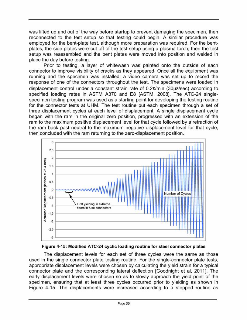
was lifted up and out of the way before startup to prevent damaging the specimen, then reconnected to the test setup so that testing could begin. A similar procedure was employed for the bent-plate test, although more preparation was required. For the bent-plates, the side plates were cut off of the test setup using a plasma torch, then the test setup was reassembled and the bent plates were moved into position and welded in place the day before testing. Prior to testing, a layer of whitewash was painted onto the outside of each connector to improve visibility of cracks as they appeared. Once all the equipment was running and the specimen was installed, a video camera was set up to record the response of one of the connectors throughout the test. The specimens were loaded in displacement control under a constant strain rate of 0.2ε/min (30με/sec) according to specified loading rates in ASTM A370 and E8 [ASTM, 2008]. The ATC-24 single-specimen testing program was used as a starting point for developing the testing routine for the connector tests at UHM. The test routine put each specimen through a set of three displacement cycles at each level of displacement. A single displacement cycle began with the ram in the original zero position, progressed with an extension of the ram to the maximum positive displacement level for that cycle followed by a retraction of the ram back past neutral to the maximum negative displacement level for that cycle, then concluded with the ram returning to the zero-displacement position.

Figure 4-15: Modified ATC-24 cyclic loading routine for steel connector plates

The displacement levels for each set of three cycles were the same as those used in the single connector plate testing routine. For the single-connector plate tests, appropriate displacement levels were chosen by calculating the yield strain for a typical connector plate and the corresponding lateral deflection [Goodnight et al, 2011]. The early displacement levels were chosen so as to slowly approach the yield point of the specimen, ensuring that at least three cycles occurred prior to yielding as shown in Figure 4-15. The displacements were increased according to a stepped routine as

Page 31

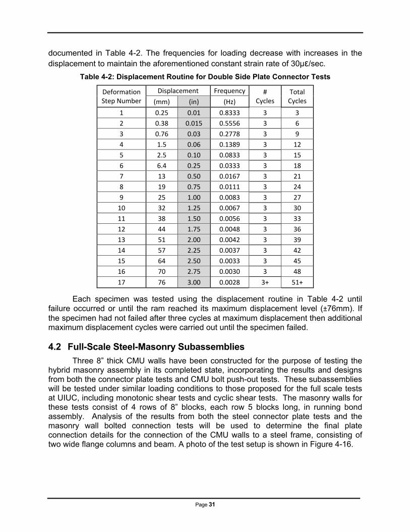
documented in Table 4-2. The frequencies for loading decrease with increases in the displacement to maintain the aforementioned constant strain rate of 30με/sec.

Table 4-2: Displacement Routine for Double Side Plate Connector Tests

Deformation Step Number

Displacement Frequency # Cycles

Total Cycles (mm) (in) (Hz)

1 0.25 0.01 0.8333 3 3

2 0.38 0.015 0.5556 3 6

3 0.76 0.03 0.2778 3 9

4 1.5 0.06 0.1389 3 12

5 2.5 0.10 0.0833 3 15

6 6.4 0.25 0.0333 3 18

7 13 0.50 0.0167 3 21

8 19 0.75 0.0111 3 24

9 25 1.00 0.0083 3 27

10 32 1.25 0.0067 3 30

11 38 1.50 0.0056 3 33

12 44 1.75 0.0048 3 36

13 51 2.00 0.0042 3 39

14 57 2.25 0.0037 3 42

15 64 2.50 0.0033 3 45

16 70 2.75 0.0030 3 48

17 76 3.00 0.0028 3+ 51+

Each specimen was tested using the displacement routine in Table 4-2 until failure occurred or until the ram reached its maximum displacement level (±76mm). If the specimen had not failed after three cycles at maximum displacement then additional maximum displacement cycles were carried out until the specimen failed.

4.2 Full-Scale Steel-Masonry Subassemblies

Three 8” thick CMU walls have been constructed for the purpose of testing the hybrid masonry assembly in its completed state, incorporating the results and designs from both the connector plate tests and CMU bolt push-out tests. These subassemblies will be tested under similar loading conditions to those proposed for the full scale tests at UIUC, including monotonic shear tests and cyclic shear tests. The masonry walls for these tests consist of 4 rows of 8” blocks, each row 5 blocks long, in running bond assembly. Analysis of the results from both the steel connector plate tests and the masonry wall bolted connection tests will be used to determine the final plate connection details for the connection of the CMU walls to a steel frame, consisting of two wide flange columns and beam. A photo of the test setup is shown in Figure 4-16.

Page 32

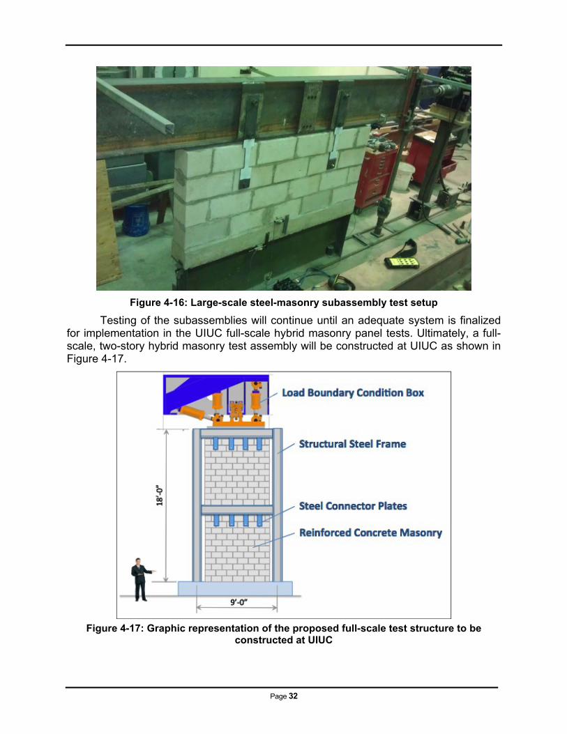
Figure 4-16: Large-scale steel-masonry subassembly test setup

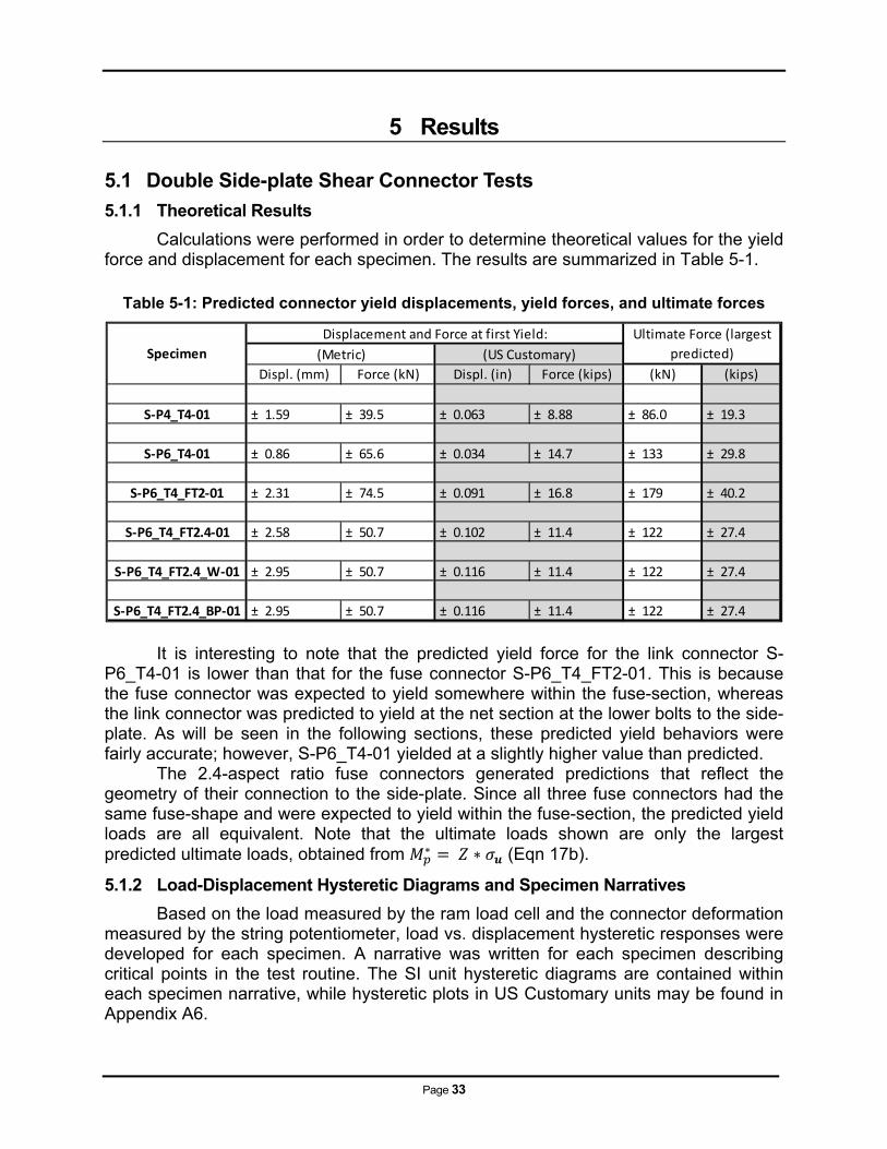
Testing of the subassemblies will continue until an adequate system is finalized for implementation in the UIUC full-scale hybrid masonry panel tests. Ultimately, a full-scale, two-story hybrid masonry test assembly will be constructed at UIUC as shown in Figure 4-17.

Figure 4-17: Graphic representation of the proposed full-scale test structure to be

constructed at UIUC

Page 33

5 Results

5.1 Double Side-plate Shear Connector Tests

5.1.1 Theoretical Results

Calculations were performed in order to determine theoretical values for the yield force and displacement for each specimen. The results are summarized in Table 5-1.

Table 5-1: Predicted connector yield displacements, yield forces, and ultimate forces

It is interesting to note that the predicted yield force for the link connector S-P6_T4-01 is lower than that for the fuse connector S-P6_T4_FT2-01. This is because the fuse connector was expected to yield somewhere within the fuse-section, whereas the link connector was predicted to yield at the net section at the lower bolts to the side-plate. As will be seen in the following sections, these predicted yield behaviors were fairly accurate; however, S-P6_T4-01 yielded at a slightly higher value than predicted. The 2.4-aspect ratio fuse connectors generated predictions that reflect the geometry of their connection to the side-plate. Since all three fuse connectors had the same fuse-shape and were expected to yield within the fuse-section, the predicted yield loads are all equivalent. Note that the ultimate loads shown are only the largest predicted ultimate loads, obtained from (Eqn 17b).

5.1.2 Load-Displacement Hysteretic Diagrams and Specimen Narratives

Based on the load measured by the ram load cell and the connector deformation measured by the string potentiometer, load vs. displacement hysteretic responses were developed for each specimen. A narrative was written for each specimen describing critical points in the test routine. The SI unit hysteretic diagrams are contained within each specimen narrative, while hysteretic plots in US Customary units may be found in Appendix A6.

S‐P4_T4‐01 ± 1.59 ± 39.5 ± 0.063 ± 8.88 ± 86.0 ± 19.3

S‐P6_T4‐01 ± 0.86 ± 65.6 ± 0.034 ± 14.7 ± 133 ± 29.8

S‐P6_T4_FT2‐01 ± 2.31 ± 74.5 ± 0.091 ± 16.8 ± 179 ± 40.2

S‐P6_T4_FT2.4‐01 ± 2.58 ± 50.7 ± 0.102 ± 11.4 ± 122 ± 27.4

S‐P6_T4_FT2.4_W‐01 ± 2.95 ± 50.7 ± 0.116 ± 11.4 ± 122 ± 27.4

S‐P6_T4_FT2.4_BP‐01 ± 2.95 ± 50.7 ± 0.116 ± 11.4 ± 122 ± 27.4

Specimen (US Customary)(Metric)

Displ. (mm) Force (kN) Displ. (in) Force (kips) (kN) (kips)

Displacement and Force at first Yield: Ultimate Force (largest

predicted)

Page 34

5.1.2.1 S-P4_T4-01

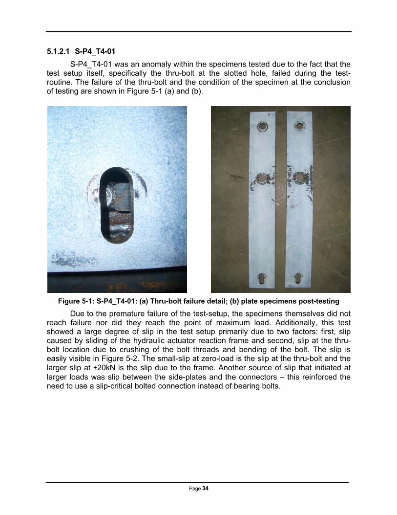
S-P4_T4-01 was an anomaly within the specimens tested due to the fact that the test setup itself, specifically the thru-bolt at the slotted hole, failed during the test-routine. The failure of the thru-bolt and the condition of the specimen at the conclusion of testing are shown in Figure 5-1 (a) and (b).

Figure 5-1: S-P4_T4-01: (a) Thru-bolt failure detail; (b) plate specimens post-testing

Due to the premature failure of the test-setup, the specimens themselves did not reach failure nor did they reach the point of maximum load. Additionally, this test showed a large degree of slip in the test setup primarily due to two factors: first, slip caused by sliding of the hydraulic actuator reaction frame and second, slip at the thru-bolt location due to crushing of the bolt threads and bending of the bolt. The slip is easily visible in Figure 5-2. The small-slip at zero-load is the slip at the thru-bolt and the larger slip at ±20kN is the slip due to the frame. Another source of slip that initiated at larger loads was slip between the side-plates and the connectors – this reinforced the need to use a slip-critical bolted connection instead of bearing bolts.

Page 35

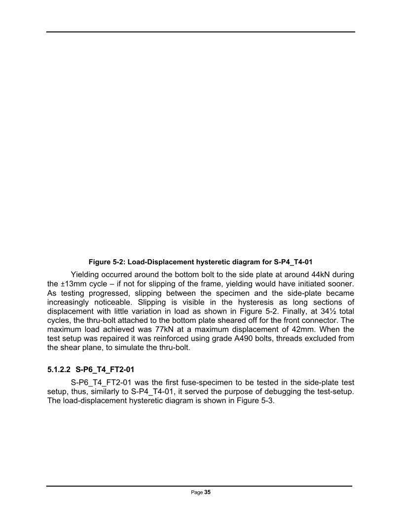
Figure 5-2: Load-Displacement hysteretic diagram for S-P4_T4-01

Yielding occurred around the bottom bolt to the side plate at around 44kN during the ±13mm cycle – if not for slipping of the frame, yielding would have initiated sooner. As testing progressed, slipping between the specimen and the side-plate became increasingly noticeable. Slipping is visible in the hysteresis as long sections of displacement with little variation in load as shown in Figure 5-2. Finally, at 34½ total cycles, the thru-bolt attached to the bottom plate sheared off for the front connector. The maximum load achieved was 77kN at a maximum displacement of 42mm. When the test setup was repaired it was reinforced using grade A490 bolts, threads excluded from the shear plane, to simulate the thru-bolt.

5.1.2.2 S-P6_T4_FT2-01

S-P6_T4_FT2-01 was the first fuse-specimen to be tested in the side-plate test setup, thus, similarly to S-P4_T4-01, it served the purpose of debugging the test-setup. The load-displacement hysteretic diagram is shown in Figure 5-3.

Page 36

Figure 5-3: Load-Displacement Hysteretic Diagram for S-P6_T4_FT2-01

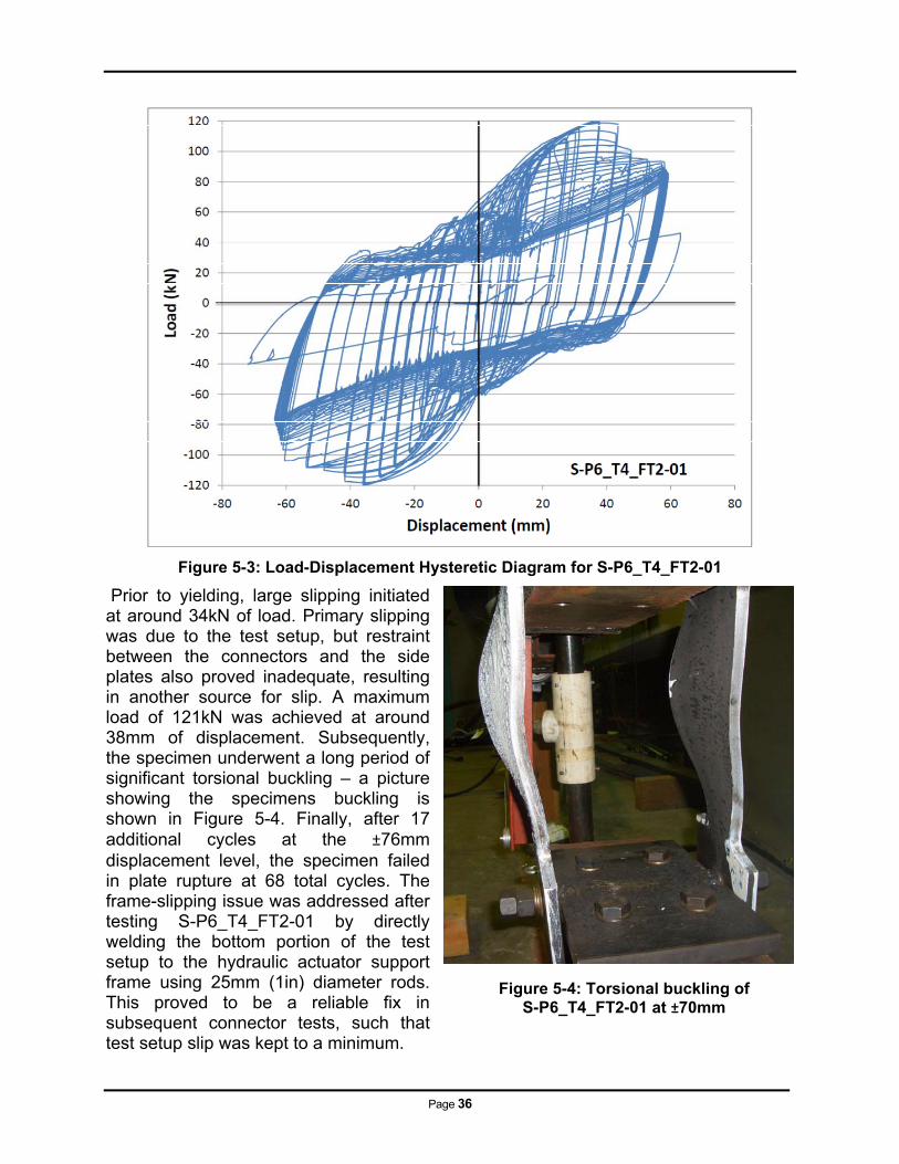
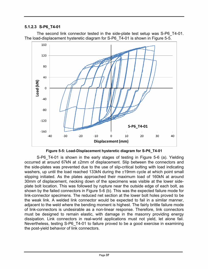
Prior to yielding, large slipping initiated at around 34kN of load. Primary slipping was due to the test setup, but restraint between the connectors and the side plates also proved inadequate, resulting in another source for slip. A maximum load of 121kN was achieved at around 38mm of displacement. Subsequently, the specimen underwent a long period of significant torsional buckling – a picture showing the specimens buckling is shown in Figure 5-4. Finally, after 17 additional cycles at the ±76mm displacement level, the specimen failed in plate rupture at 68 total cycles. The frame-slipping issue was addressed after testing S-P6_T4_FT2-01 by directly welding the bottom portion of the test setup to the hydraulic actuator support frame using 25mm (1in) diameter rods. This proved to be a reliable fix in subsequent connector tests, such that test setup slip was kept to a minimum.

Figure 5-4: Torsional buckling of S-P6_T4_FT2-01 at ±70mm

Page 37

5.1.2.3 S-P6_T4-01

The second link connector tested in the side-plate test setup was S-P6_T4-01. The load-displacement hysteretic diagram for S-P6_T4-01 is shown in Figure 5-5.

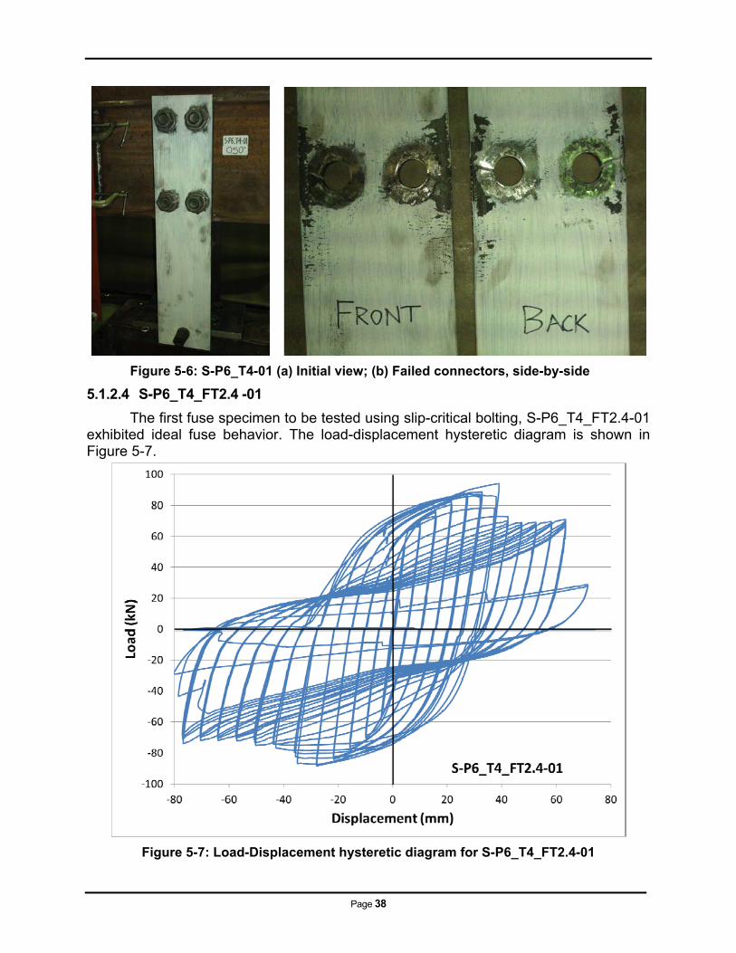
Figure 5-5: Load-Displacement hysteretic diagram for S-P6_T4-01

S-P6_T4-01 is shown in the early stages of testing in Figure 5-6 (a). Yielding occurred at around 67kN at ±2mm of displacement. Slip between the connectors and the side-plates was prevented due to the use of slip-critical bolting with load indicating washers, up until the load reached 133kN during the ±19mm cycle at which point small slipping initiated. As the plates approached their maximum load of 160kN at around 30mm of displacement, necking down of the specimens was visible at the lower side-plate bolt location. This was followed by rupture near the outside edge of each bolt, as shown by the failed connectors in Figure 5-6 (b). This was the expected failure mode for link-connector specimens. The reduced net section at the lower bolt holes proved to be the weak link. A welded link connector would be expected to fail in a similar manner, adjacent to the weld where the bending moment is highest. The fairly brittle failure mode of link-connectors is undesirable as a non-linear response. Therefore, link connectors must be designed to remain elastic, with damage in the masonry providing energy dissipation. Link connectors in real-world applications must not yield, let alone fail. Nevertheless, testing S-P6_T4-01 to failure proved to be a good exercise in examining the post-yield behavior of link connectors.

Page 38

Figure 5-6: S-P6_T4-01 (a) Initial view; (b) Failed connectors, side-by-side

5.1.2.4 S-P6_T4_FT2.4 -01

The first fuse specimen to be tested using slip-critical bolting, S-P6_T4_FT2.4-01 exhibited ideal fuse behavior. The load-displacement hysteretic diagram is shown in Figure 5-7.

Figure 5-7: Load-Displacement hysteretic diagram for S-P6_T4_FT2.4-01

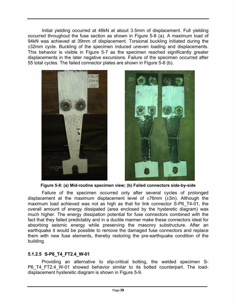
Page 39

Initial yielding occurred at 48kN at about 3.5mm of displacement. Full yielding occurred throughout the fuse section as shown in Figure 5-8 (a). A maximum load of 94kN was achieved at 39mm of displacement. Torsional buckling initiated during the ±32mm cycle. Buckling of the specimen induced uneven loading and displacements. This behavior is visible in Figure 5-7 as the specimen reached significantly greater displacements in the later negative excursions. Failure of the specimen occurred after 55 total cycles. The failed connector plates are shown in Figure 5-8 (b).

Figure 5-8: (a) Mid-routine specimen view; (b) Failed connectors side-by-side

Failure of the specimen occurred only after several cycles of prolonged displacement at the maximum displacement level of ±76mm (±3in). Although the maximum load achieved was not as high as that for link connector S-P6_T4-01, the overall amount of energy dissipated (area enclosed by the hysteretic diagram) was much higher. The energy dissipation potential for fuse connectors combined with the fact that they failed predictably and in a ductile manner make these connectors ideal for absorbing seismic energy while preserving the masonry substructure. After an earthquake it would be possible to remove the damaged fuse connectors and replace them with new fuse elements, thereby restoring the pre-earthquake condition of the building.

5.1.2.5 S-P6_T4_FT2.4_W-01

Providing an alternative to slip-critical bolting, the welded specimen S-P6_T4_FT2.4_W-01 showed behavior similar to its bolted counterpart. The load-displacement hysteretic diagram is shown in Figure 5-9.

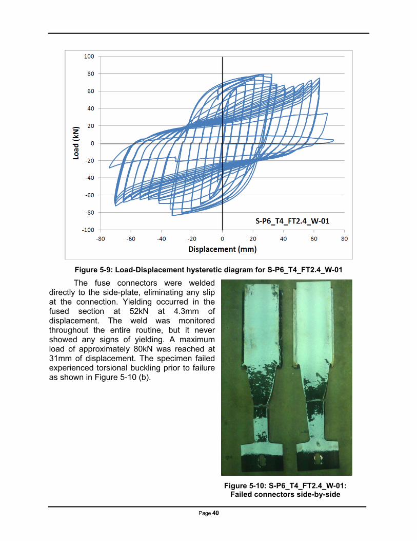
Page 40

Figure 5-9: Load-Displacement hysteretic diagram for S-P6_T4_FT2.4_W-01

The fuse connectors were welded directly to the side-plate, eliminating any slip at the connection. Yielding occurred in the fused section at 52kN at 4.3mm of displacement. The weld was monitored throughout the entire routine, but it never showed any signs of yielding. A maximum load of approximately 80kN was reached at 31mm of displacement. The specimen failed experienced torsional buckling prior to failure as shown in Figure 5-10 (b).

Figure 5-10: S-P6_T4_FT2.4_W-01: Failed connectors side-by-side

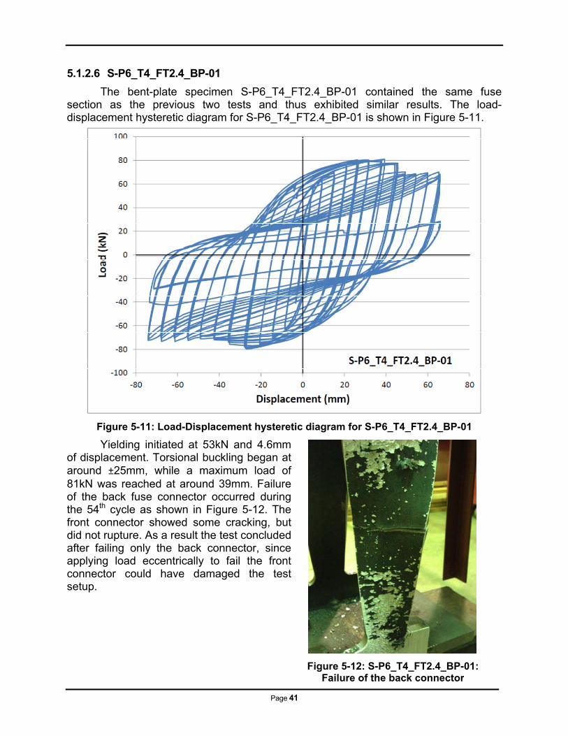
Page 41

5.1.2.6 S-P6_T4_FT2.4_BP-01

The bent-plate specimen S-P6_T4_FT2.4_BP-01 contained the same fuse section as the previous two tests and thus exhibited similar results. The load-displacement hysteretic diagram for S-P6_T4_FT2.4_BP-01 is shown in Figure 5-11.

Figure 5-11: Load-Displacement hysteretic diagram for S-P6_T4_FT2.4_BP-01

Yielding initiated at 53kN and 4.6mm of displacement. Torsional buckling began at around ±25mm, while a maximum load of 81kN was reached at around 39mm. Failure of the back fuse connector occurred during the 54th cycle as shown in Figure 5-12. The front connector showed some cracking, but did not rupture. As a result the test concluded after failing only the back connector, since applying load eccentrically to fail the front connector could have damaged the test setup.

Figure 5-12: S-P6_T4_FT2.4_BP-01:

Failure of the back connector

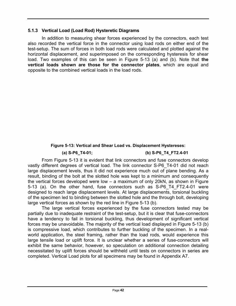
Page 42

5.1.3 Vertical Load (Load Rod) Hysteretic Diagrams

In addition to measuring shear forces experienced by the connectors, each test also recorded the vertical force in the connector using load rods on either end of the test-setup. The sum of forces in both load rods were calculated and plotted against the horizontal displacement, and superimposed on the corresponding hysteresis for shear load. Two examples of this can be seen in Figure 5-13 (a) and (b). Note that the vertical loads shown are those for the connector plates, which are equal and opposite to the combined vertical loads in the load rods.

Figure 5-13: Vertical and Shear Load vs. Displacement Hystereses:

(a) S-P6_T4-01; (b) S-P6_T4_FT2.4-01

From Figure 5-13 it is evident that link connectors and fuse connectors develop vastly different degrees of vertical load. The link connector S-P6_T4-01 did not reach large displacement levels, thus it did not experience much out of plane bending. As a result, binding of the bolt at the slotted hole was kept to a minimum and consequently the vertical forces developed were low – a maximum of only 20kN, as shown in Figure 5-13 (a). On the other hand, fuse connectors such as S-P6_T4_FT2.4-01 were designed to reach large displacement levels. At large displacements, torsional buckling of the specimen led to binding between the slotted hole and the through bolt, developing large vertical forces as shown by the red line in Figure 5-13 (b). The large vertical forces experienced by the fuse connectors tested may be partially due to inadequate restraint of the test-setup, but it is clear that fuse-connectors have a tendency to fail in torsional buckling, thus development of significant vertical forces may be unavoidable. The majority of the vertical load displayed in Figure 5-13 (b) is compressive load, which contributes to further buckling of the specimen. In a real-world application, the steel framing, rather than the load rods, would experience this large tensile load or uplift force. It is unclear whether a series of fuse-connectors will exhibit the same behavior, however, so speculation on additional connection detailing necessitated by uplift forces should be withheld until tests on connectors in series are completed. Vertical Load plots for all specimens may be found in Appendix A7.

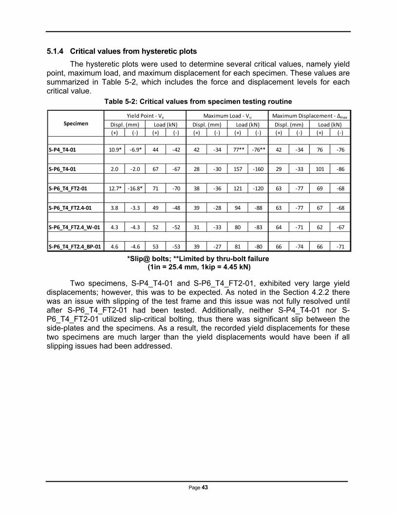
Page 43

5.1.4 Critical values from hysteretic plots

The hysteretic plots were used to determine several critical values, namely yield point, maximum load, and maximum displacement for each specimen. These values are summarized in Table 5-2, which includes the force and displacement levels for each critical value.

Table 5-2: Critical values from specimen testing routine

*Slip@ bolts; **Limited by thru-bolt failure

(1in = 25.4 mm, 1kip = 4.45 kN)

Two specimens, S-P4_T4-01 and S-P6_T4_FT2-01, exhibited very large yield displacements; however, this was to be expected. As noted in the Section 4.2.2 there was an issue with slipping of the test frame and this issue was not fully resolved until after S-P6_T4_FT2-01 had been tested. Additionally, neither S-P4_T4-01 nor S-P6_T4_FT2-01 utilized slip-critical bolting, thus there was significant slip between the side-plates and the specimens. As a result, the recorded yield displacements for these two specimens are much larger than the yield displacements would have been if all slipping issues had been addressed.

(+) (‐) (+) (‐) (+) (‐) (+) (‐) (+) (‐) (+) (‐)

S‐P4_T4‐01 10.9* ‐6.9* 44 ‐42 42 ‐34 77** ‐76** 42 ‐34 76 ‐76

S‐P6_T4‐01 2.0 ‐2.0 67 ‐67 28 ‐30 157 ‐160 29 ‐33 101 ‐86

S‐P6_T4_FT2‐01 12.7* ‐16.8* 71 ‐70 38 ‐36 121 ‐120 63 ‐77 69 ‐68

S‐P6_T4_FT2.4‐01 3.8 ‐3.3 49 ‐48 39 ‐28 94 ‐88 63 ‐77 67 ‐68

S‐P6_T4_FT2.4_W‐01 4.3 ‐4.3 52 ‐52 31 ‐33 80 ‐83 64 ‐71 62 ‐67

S‐P6_T4_FT2.4_BP‐01 4.6 ‐4.6 53 ‐53 39 ‐27 81 ‐80 66 ‐74 66 ‐71

Yield Point ‐ Vy Maximum Load ‐ Vu Maximum Displacement ‐ ∆max

Displ. (mm) Load (kN) Displ. (mm) Load (kN) Displ. (mm) Load (kN)Specimen

Page 44

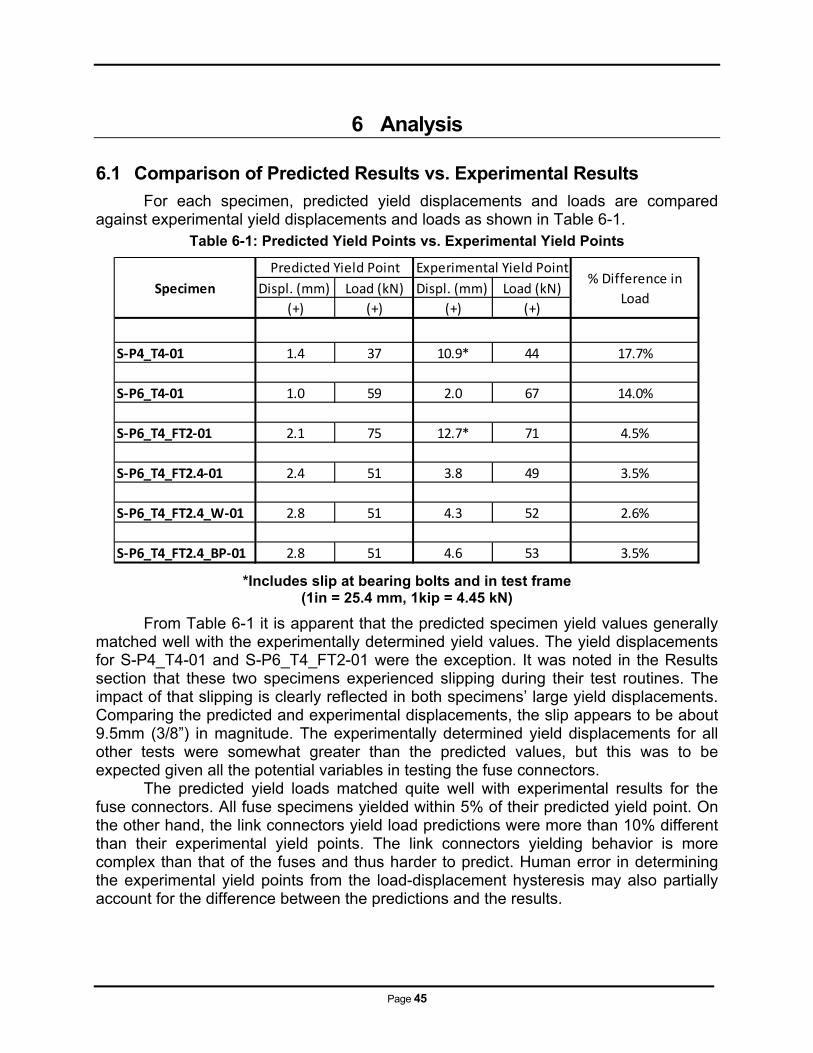
Page 45

6 Analysis

6.1 Comparison of Predicted Results vs. Experimental Results

For each specimen, predicted yield displacements and loads are compared against experimental yield displacements and loads as shown in Table 6-1.

Table 6-1: Predicted Yield Points vs. Experimental Yield Points

*Includes slip at bearing bolts and in test frame (1in = 25.4 mm, 1kip = 4.45 kN)

From Table 6-1 it is apparent that the predicted specimen yield values generally matched well with the experimentally determined yield values. The yield displacements for S-P4_T4-01 and S-P6_T4_FT2-01 were the exception. It was noted in the Results section that these two specimens experienced slipping during their test routines. The impact of that slipping is clearly reflected in both specimens’ large yield displacements. Comparing the predicted and experimental displacements, the slip appears to be about 9.5mm (3/8”) in magnitude. The experimentally determined yield displacements for all other tests were somewhat greater than the predicted values, but this was to be expected given all the potential variables in testing the fuse connectors. The predicted yield loads matched quite well with experimental results for the fuse connectors. All fuse specimens yielded within 5% of their predicted yield point. On the other hand, the link connectors yield load predictions were more than 10% different than their experimental yield points. The link connectors yielding behavior is more complex than that of the fuses and thus harder to predict. Human error in determining the experimental yield points from the load-displacement hysteresis may also partially account for the difference between the predictions and the results.

Displ. (mm) Load (kN) Displ. (mm) Load (kN)

(+) (+) (+) (+)

S‐P4_T4‐01 1.4 37 10.9* 44

S‐P6_T4‐01 1.0 59 2.0 67

S‐P6_T4_FT2‐01 2.1 75 12.7* 71

S‐P6_T4_FT2.4‐01 2.4 51 3.8 49

S‐P6_T4_FT2.4_W‐01 2.8 51 4.3 52

S‐P6_T4_FT2.4_BP‐01 2.8 51 4.6 53

Specimen

Predicted Yield Point Experimental Yield Point

3.5%

% Difference in

Load

4.5%

3.5%

2.6%

17.7%

14.0%

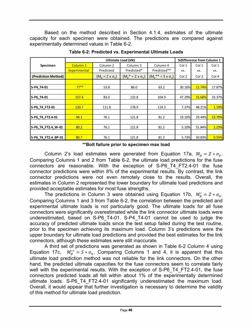
Page 46

Based on the method described in Section 4.1.4, estimates of the ultimate capacity for each specimen were obtained. The predictions are compared against experimentally determined values in Table 6-2.

Table 6-2: Predicted vs. Experimental Ultimate Loads

**Bolt failure prior to specimen max load

Column 2’s load estimates were generated from Equation 17a, . Comparing Columns 1 and 2 from Table 6-2, the ultimate load predictions for the fuse connectors are reasonable. With the exception of S-P6_T4_FT2.4-01 the fuse connector predictions were within 8% of the experimental results. By contrast, the link connector predictions were not even remotely close to the results. Overall, the estimates in Column 2 represented the lower boundary for ultimate load predictions and provided acceptable estimates for most fuse strengths.

The predictions in Column 3 were obtained using Equation 17b, . Comparing Columns 1 and 3 from Table 6-2, the correlation between the predicted and experimental ultimate loads is not particularly good. The ultimate loads for all fuse connectors were significantly overestimated while the link connector ultimate loads were underestimated, based on S-P6_T4-01. S-P4_T4-01 cannot be used to judge the accuracy of predicted ultimate loads since the test setup failed during the test routine, prior to the specimen achieving its maximum load. Column 3’s predictions were the upper boundary for ultimate load predictions and provided the best estimates for the link connectors, although these estimates were still inaccurate. A third set of predictions was generated as shown in Table 6-2 Column 4 using Equation 17c, . Comparing Columns 1 and 4, it is apparent that this ultimate load prediction method was not reliable for the link connectors. On the other hand, the predicted ultimate capacities for the fuse connectors seem to correlate fairly well with the experimental results. With the exception of S-P6_T4_FT2.4-01, the fuse connectors predicted loads all fell within about 1% of the experimentally determined ultimate loads. S-P6_T4_FT2.4-01 significantly underestimated the maximum load. Overall, it would appear that further investigation is necessary to determine the validity of this method for ultimate load prediction.

Column 1 Column 2 Column 3 Column 4 Col 1 Col 1 Col 1

Experimental Predicted Predicted* Predicted** vs. vs. vs.

(Prediction Method) (Mp = Z x σy) (Mp* = Z x σu) (Mp** = S x σu) Col 2 Col 3 Col 4

S‐P4_T4‐01 77** 53.8 86.0 63.2 30.16% 11.74% 17.87%

S‐P6_T4‐01 157.4 83.0 132.8 104.9 47.29% 15.66% 33.37%

S‐P6_T4_FT2‐01 120.7 111.8 178.9 119.3 7.37% 48.21% 1.19%

S‐P6_T4_FT2.4‐01 94.1 76.1 121.8 81.2 19.10% 29.44% 13.70%

S‐P6_T4_FT2.4_W‐01 80.2 76.1 121.8 81.2 5.10% 51.84% 1.23%

S‐P6_T4_FT2.4_BP‐01 80.7 76.1 121.8 81.2 5.73% 50.83% 0.55%

%Difference from Column 1

Specimen

Ultimate Load (kN)

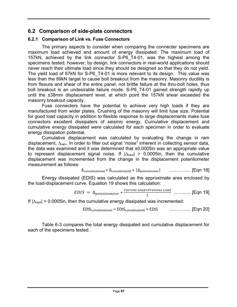
Page 47

6.2 Comparison of side-plate connectors

6.2.1 Comparison of Link vs. Fuse Connectors

The primary aspects to consider when comparing the connecter specimens are maximum load achieved and amount of energy dissipated. The maximum load of 157kN, achieved by the link connector S-P6_T4-01, was the highest among the specimens tested; however, by design, link connectors in real-world applications should never reach their ultimate load since they should be designed so that they do not yield. The yield load of 67kN for S-P6_T4-01 is more relevant to its design. This value was less than the 89kN target to cause bolt breakout from the masonry. Masonry ductility is from flexure and shear of the entire panel, not brittle failure at the thru-bolt holes, thus bolt breakout is an undesirable failure mode. S-P6_T4-01 gained strength rapidly up until the ±38mm displacement level, at which point the 157kN shear exceeded the masonry breakout capacity. Fuse connecters have the potential to achieve very high loads if they are manufactured from wider plates. Crushing of the masonry will limit fuse size. Potential for good load capacity in addition to flexible response to large displacements make fuse connectors excellent dissipaters of seismic energy. Cumulative displacement and cumulative energy dissipated were calculated for each specimen in order to evaluate energy dissipation potential. Cumulative displacement was calculated by evaluating the change in ram displacement, ∆ram. In order to filter out signal “noise” inherent in collecting sensor data, the data was examined and it was determined that ±0.0005in was an appropriate value to represent displacement signal noise. If |∆ram| > 0.0005in, then the cumulative displacement was incremented from the change in the displacement potentiometer measurement as follows:

δcumulative(new) = δcumulative(old) + |∆potentiometer| ………...... [Eqn 18]

Energy dissipated (EDIS) was calculated as the approximate area enclosed by the load-displacement curve. Equation 19 shows this calculation:

∆ ……...... [Eqn 19]

If |∆ram| > 0.0005in, then the cumulative energy dissipated was incremented:

EDIScumulative(new) = EDIScumulative(old) + EDIS ………...... [Eqn 20]

Table 6-3 compares the total energy dissipated and cumulative displacement for each of the specimens tested.

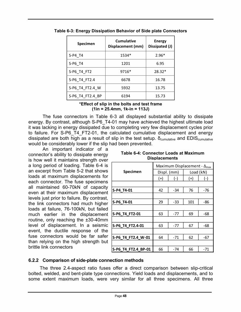
Page 48

Table 6-3: Energy Dissipation Behavior of Side plate Connectors

Specimen Cumulative

Displacement (mm) Energy

Dissipated (J)

S‐P4_T4 1534* 2.96*

S‐P6_T4 1201 6.95

S‐P6_T4_FT2 9716* 28.32*

S‐P6_T4_FT2.4 6678 16.78

S‐P6_T4_FT2.4_W 5932 13.75

S‐P6_T4_FT2.4_BP 6194 15.73

*Effect of slip in the bolts and test frame (1in = 25.4mm, 1k-in = 113J)

The fuse connectors in Table 6-3 all displayed substantial ability to dissipate energy. By contrast, although S-P6_T4-01 may have achieved the highest ultimate load it was lacking in energy dissipated due to completing very few displacement cycles prior to failure. For S-P6_T4_FT2-01, the calculated cumulative displacement and energy dissipated are both high as a result of slip in the test setup. δcumulative and EDIScumulative would be considerably lower if the slip had been prevented. An important indicator of a connector’s ability to dissipate energy is how well it maintains strength over a long period of loading. Table 6-4 is an excerpt from Table 5-2 that shows loads at maximum displacements for each connector. The fuse specimens all maintained 60-70kN of capacity even at their maximum displacement levels just prior to failure. By contrast, the link connectors had much higher loads at failure, 76-100kN, but failed much earlier in the displacement routine, only reaching the ±30-40mm level of displacement. In a seismic event, the ductile response of the fuse connectors would be far safer than relying on the high strength but brittle link connectors

6.2.2 Comparison of side-plate connection methods

The three 2.4-aspect ratio fuses offer a direct comparison between slip-critical bolted, welded, and bent-plate type connections. Yield loads and displacements, and to some extent maximum loads, were very similar for all three specimens. All three

Table 6-4: Connector Loads at Maximum Displacements

(+) (‐) (+) (‐)

S‐P4_T4‐01 42 ‐34 76 ‐76

S‐P6_T4‐01 29 ‐33 101 ‐86

S‐P6_T4_FT2‐01 63 ‐77 69 ‐68

S‐P6_T4_FT2.4‐01 63 ‐77 67 ‐68

S‐P6_T4_FT2.4_W‐01 64 ‐71 62 ‐67

S‐P6_T4_FT2.4_BP‐01 66 ‐74 66 ‐71

Displ. (mm) Load (kN)Specimen

Maximum Displacement ‐ ∆max

Page 49

specimens completed between 53 to 55 total displacement cycles and ultimately failed due to lateral torsional buckling. In terms of energy dissipated, S-P6_T4_FT2.4-01 achieved a higher maximum load and slightly more cumulative displacement, thus it dissipated slightly more energy. The side plate welded specimen dissipated the least energy of the three fuses, which was to be expected considering it had the least flexible connection type. All three connection types proved to be viable options for fuse connector specimens.

Based on the results of S-P6_T4-01, welded connection methods may be preferable for link connectors as opposed to bolted connection methods. Yielding at the bolt holes greatly reduced the yield force for S-P6_T4-01; if the specimen had been welded to the side-plates instead of bolted, then the connector section would not have had such an obvious weak-point. A bent-plate type of link connector, so long as it can adequately resist yield loads, should be just as advantageous as a side plate welded link connector. 6.3 ATC-24 Connector Plate Analysis

The goal of the ATC-24 connector plate analysis was to obtain a set of parameters for each specimen that could be used to develop analytical models. ATC-24 guidelines recommend obtaining a full set of performance parameters, to include specimen strength characteristics, stiffness characteristics, deformation capacity, and energy dissipation for each excursion of the specimen loading history [ATC, 1992]. Table 6-5 shows the ATC-24 spreadsheet developed for S-P6_T4-01. All other connector spreadsheets can be found in Appendix A8.

All of the experimentally determined values listed in the tables have been normalized with respect to analytically determined values of yield force, Qy, and yield displacement, δy, based on an assumed material yield strength, Fy, of 50 ksi. Note that Qy = Vy = the 2-connector yield force. Column 1 lists the entry number for each row of data, starting with 1 at the first excursion and increasing with each subsequent excursion. Column 2 lists the absolute value of the programmed actuator displacement level corresponding to each excursion. Column 3 lists the excursion number from which each row of data was extracted, followed by a positive sign (+) or a negative sign (-) noting either a compressive or a tensile force in the actuator load cell, respectively. The maximum deflection, δ, reached by a specimen during a given excursion is listed in Column 4. The deflection at the start of each excursion, δ0, is listed in Column 5. The difference between this value and the deflection at the start of the subsequent excursion (i.e. the point at which the load on the specimen changed signs) represents the plastic deformation range, Δδpm, for each excursion and is listed in Column 6.

The load, Q, corresponding to the maximum deflection in each excursion is given in Column 7, while Column 8 lists the maximum overall load, Qmax, attained by the specimen during each excursion. The initial loading stiffness, K0, and initial unloading stiffness, K, are given in Columns 9 and 10, respectively. These values correspond to the slope (change in load vs. change in displacement) of the first 20 (loading) and last 20 (unloading) data values in each excursion. Finally, the area under the hysteretic loop of each excursion was used to quantify the specimen energy dissipation, as listed in Column 11.

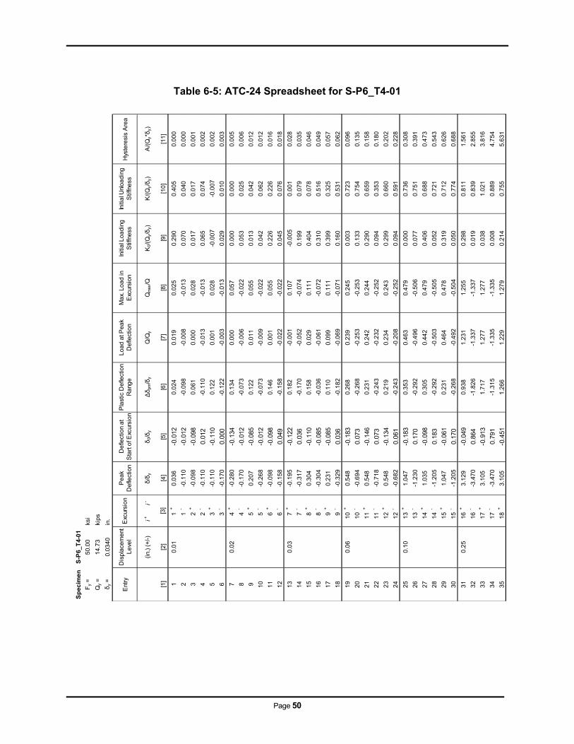
Page 50

Table 6-5: ATC-24 Spreadsheet for S-P6_T4-01

Sp

ec

ime

nS

-P6

_T

4-0

1

Fy

=5

0.0

0ks

i

Qy

=1

4.7

3ki

ps

δy

=0

.03

40

in.

Ent

ryD

isp

lace

me

nt

Le

vel

Pe

ak

De

flect

ion

De

flect

ion

at

Sta

rt o

f Exc

ursi

on

Pla

stic

De

flect

ion

Ra

nge

Lo

ad

at P

ea

k D

efle

ctio

nM

ax.

Lo

ad

in

Exc

ursi

on

Initi

al L

oa

din

g

Stif

fne

ssIn

itia

l Unl

oa

din

g

Stif

fne

ssH

yste

resi

s A

rea

(in.

) (+

/-)

i+i-

δ/δ

yδ

0/δ

yΔδ

pm/δ

yQ

/Qy

Qm

ax/Q

K0/

(Qy/δ

y)K

/(Q

y/δ

y)A

/(Q

y*δ

y)

[1]

[2]

[4]

[5]

[6]

[7]

[8]

[9]

[10

][1

1]

10

.01

1+

0.0

36

-0.0

120

.02

40

.01

90

.02

50

.29

00

.40

50

.00

0

21

--0

.11

0-0

.012

-0.0

98

-0.0

08

-0.0

13

0.0

70

0.0

40

0.0

00

32

+-0

.09

8-0

.098

0.0

61

0.0

00

0.0

28

0.0

17

0.0

17

0.0

01

42

--0

.11

00.

012

-0.1

10

-0.0

13

-0.0

13

0.0

65

0.0

74

0.0

02

53

+-0

.11

0-0

.110

0.1

22

0.0

01

0.0

28

-0.0

07

-0.0

07

0.0

02

63

--0

.17

00.

000

-0.1

22

-0.0

03

-0.0

13

0.0

29

0.0

10

0.0

03

70

.02

4+

-0.2

80

-0.1

340

.13

40

.00

00

.05

70

.00

00

.00

00

.00

5

84

--0

.17

0-0

.012

-0.0

73

-0.0

06

-0.0

22

0.0

53

0.0

25

0.0

06

95

+0

.20

7-0

.085

0.1

22

0.0

11

0.0

55

0.0

13

0.0

42

0.0

12

10

5-

-0.2

68

-0.0

12-0

.07

3-0

.00

9-0

.02

20

.04

20

.06

20

.01

2

11

6+

-0.0

98

-0.0

980

.14

60

.00

10

.05

50

.22

60

.22

60

.01

6

12

6-

-0.1

58

0.04

9-0

.15

8-0

.02

2-0

.02

20

.04

50

.07

60

.01

8

13

0.0

37

+-0

.19

5-0

.122

0.1

82

-0.0

01

0.1

07

-0.0

05

0.0

01

0.0

28

14

7-

-0.3

17

0.03

6-0

.17

0-0

.05

2-0

.07

40

.19

90

.07

90

.03

5

15

8+

0.3

04

-0.1

100

.15

80

.02

90

.11

10

.40

40

.07

80

.04

6

16

8-

-0.3

04

-0.0

85-0

.03

6-0

.06

1-0

.07

20

.31

00

.51

60

.04

9

17

9+

0.2

31

-0.0

850

.11

00

.09

90

.11

10

.39

90

.32

50

.05

7

18

9-

-0.3

29

0.03

6-0

.18

2-0

.06

9-0

.07

10

.16

00

.53

10

.06

2

19

0.0

61

0+

0.5

48

-0.1

830

.26

80

.23

90

.24

50

.00

30

.72

30

.09

6

20

10

--0

.69

40.

073

-0.2

68

-0.2

53

-0.2

53

0.1

33

0.7

54

0.1

35

21

11

+0

.54

8-0

.146

0.2

31

0.2

42

0.2

44

0.2

90

0.6

59

0.1

58

22

11

--0

.71

80.

073

-0.2

43

-0.2

32

-0.2

52

0.0

94

0.3

53

0.1

80

23

12

+0

.54

8-0

.134

0.2

19

0.2

34

0.2

43

0.2

99

0.6

60

0.2

02

24

12

--0

.68

20.

061

-0.2

43

-0.2

08

-0.2

52

0.0

94

0.5

91

0.2

28

25

0.1

01

3+

1.0

47

-0.1

830

.35

30

.46

30

.47

90

.00

00

.73

60

.30

8

26

13

--1

.23

00.

170

-0.2

92

-0.4

96

-0.5

06

0.0

77

0.7

51

0.3

91

27

14

+1

.03

5-0

.098

0.3

05

0.4

42

0.4

79

0.4

06

0.6

88

0.4

73

28

14

--1

.20

50.

183

-0.2

92

-0.5

03

-0.5

05

0.0

52

0.7

21

0.5

43

29

15

+1

.04

7-0

.061

0.2

31

0.4

64

0.4

78

0.3

19

0.7

12

0.6

26

30

15

--1

.20

50.

170

-0.2

68

-0.4

92

-0.5

04

0.0

50

0.7

74

0.6

88

31

0.2

51

6+

3.1

29

-0.0

490

.93

81

.23

11

.25

50

.29

80

.81

11

.56

1

32

16

--3

.47

00.

864

-1.8

26

-1.3

37

-1.3

37

0.0

19

0.8

39

2.8

55

33

17

+3

.10

5-0

.913

1.7

17

1.2

77

1.2

77

0.0

38

1.0

21

3.8

16

34

17

--3

.47

00.

791

-1.3

15

-1.3

35

-1.3

35

0.0

08

0.8

89

4.7

54

35

18

+3

.10

5-0

.451

1.2

66

1.2

29

1.2

79

0.2

14

0.7

55

5.6

31

Exc

ursi

on

[3]

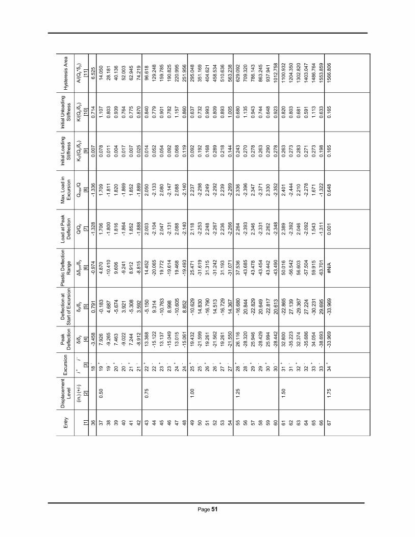
Page 51

Ent

ryD

isp

lace

men

t L

eve

lP

eak

De

flect

ion

De

flect

ion

at

Sta

rt o

f Exc

ursi

on

Pla

stic

De

flect

ion

Ra

nge

Lo

ad

at P

ea

k D

efle

ctio

nM

ax.

Lo

ad in

E

xcur

sio

nIn

itia

l Lo

ad

ing

S

tiffn

ess

Initi

al U

nlo

ad

ing

Stif

fne

ssH

yste

resi

s A

rea

(in.

) (+

/-)i+

i-δ/δ

yδ 0

/δy

Δδ p

m/δ

yQ

/Qy

Qm

ax/Q

K0/

(Qy/δ

y)K

/(Q

y/δ

y)A

/(Q

y*δ

y)

[1]

[2]

[4]

[5]

[6]

[7]

[8]

[9]

[10]

[11

]

36

18

--3

.458

0.79

1-0

.97

4-1

.32

8-1

.33

60

.00

70

.714

6.5

25

37

0.5

01

9+

7.9

26

-0.1

834.

87

01

.70

61

.70

90

.07

81

.107

14.0

50

38

19

--9

.265

4.68

7-1

0.4

10

-1.8

00

-1.8

11

0.0

11

0.8

0328

.18

1

39

20

+7

.46

3-5

.674

9.6

06

1.8

16

1.8

20

0.0

04

0.9

3940

.13

6

40

20

--9

.022

3.92

1-9

.24

1-1

.86

4-1

.86

90

.01

70

.764

52.0

03

41

21

+7

.24

4-5

.308

8.9

12

1.8

52

1.8

52

0.0

07

0.7

7562

.94

5

42

21

--8

.912

3.59

2-8

.81

5-1

.88

8-1

.88

90

.02

50

.870

74.2

19

43

0.7

52

2+

13

.36

8-5

.150

14.

45

22

.00

32

.05

00

.01

40

.840

96.6

18

44

22

--1

5.1

22

9.31

4-2

0.0

65

-2.1

04

-2.1

33

0.0

52

0.7

7912

9.2

48

45

23

+1

3.1

37

-10.

763

19.

77

22

.04

72

.08

00

.05

40

.901

159

.78

5

46

23

--1

5.0

49

8.99

8-1

9.6

14

-2.1

31

-2.1

47

0.0

92

0.7

8219

0.8

25

47

24

+1

3.0

15

-10.

605

19.

46

82

.08

82

.08

80

.06

81

.157

220

.99

5

48

24

--1

5.0

61

8.85

2-1

9.4

93

-2.1

40

-2.1

40

0.1

19

0.8

6025

1.9

56

49

1.0

02

5+

19

.43

2-1

0.62

92

5.4

71

2.1

18

2.2

37

0.0

92

0.6

3729

5.0

48

50

25

--2

1.5

99

14.8

30-3

1.6

19

-2.2

53

-2.2

98

0.1

92

0.7

3235

1.1

69

51

26

+1

9.2

61

-16.

790

31.

31

52

.24

82

.24

90

.16

80

.993

404

.62

1

52

26

--2

1.5

62

14.5

13-3

1.2

42

-2.2

67

-2.2

92

0.2

89

0.8

0945

8.5

34

53

27

+1

9.2

61

-16.

729

31.

19

32

.23

62

.23

90

.21

80

.893

510

.63

6

54

27

--2

1.5

50

14.3

67-3

1.0

71

-2.2

66

-2.2

69

0.1

44

1.0

0556

3.2

38

55

1.2

52

8+

26

.11

6-1

6.68

03

7.5

36

2.2

64

2.3

36

0.2

43

0.6

8062

9.0

92

56

28

--2

8.3

20

20.8

44-4

3.6

85

-2.3

93

-2.3

96

0.2

70

1.1

3570

9.3

20

57

29

+2

5.9

46

-22.

829

43.

47

82

.34

62

.34

70

.27

80

.943

786

.14

3

58

29

--2

8.4

29

20.6

49-4

3.4

54

-2.3

31

-2.3

71

0.2

63

0.7

4486

3.2

45

59

30

+2

5.9

94

-22.

817

43.

44

22

.26

22

.33

00

.29

00

.648

937

.94

1

60

30

--2

8.4

42

20.6

13-4

3.4

90

-2.3

48

-2.3

52

0.2

78

0.9

231

012

.758

61

1.5

03

1+

32

.80

0-2

2.86

55

0.0

16

2.3

89

2.4

01

0.2

63

0.8

201

100

.932

62

31

--3

5.2

23

27.1

39-5

6.5

42

-2.3

92

-2.4

44

0.2

73

0.8

031

204

.350

63

32

+3

2.3

74

-29.

367

56.

60

32

.04

62

.21

00

.28

30

.681

13

02.8

20

64

32

--3

5.6

86

27.2

24-5

7.5

04

-2.0

92

-2.2

78

0.2

71

0.5

911

403

.047

65

33

+3

4.0

54

-30.

231

59.

91

51

.54

31

.67

10

.27

31

.113

14

86.7

64

66

33

--3

8.6

93

29.6

95-6

3.7

01

-1.3

11

-1.3

22

0.1

98

0.6

331

553

.859

67

1.7

53

4+

-33

.96

9-3

3.96

9#

N/A

0.0

01

0.6

48

0.1

65

0.1

651

566

.806

Exc

ursi

on

[3]

Page 52

Page 53

7 Conclusions / Recommendations

Recommendations are presented for the design of side-plate fuse connectors.

Slip-critical bolting, welding, and bent-plate connections are all viable options for fuse-type side plate connectors.

Side plate connectors are the most practical type of connector developed thus far, having potentially high load and energy dissipation capabilities.

A welded connection is most likely preferable to a bolted connection for side-plate link-connectors.

o A minimum of two additional tests are recommended for link connectors: a test of specimens welded to the side-plates and a test in the bent-plate configuration. Testing these two connection types should confirm that they are superior to a slip-critical bolted connection, which significantly reduces the net section at the plastic hinge and lowers the yield load as a result.

Further testing may be necessary to develop more accurate predictions for

ultimate load for both link connectors and fuse connectors.

Repetition of the most relevant tests may be appropriate to confirm the repeatability of results.

Tests of plasma-cut fuses should be performed to compare with the test results from milled specimens.

Further testing is recommended to investigate the effects of the interaction of a line of multiple thru-bolted connections in a single CMU wall panel. Testing a series of fuses installed on the full-scale steel-masonry subassemblies should address this concern.

Page 54

Page 55

8 References

Abrams (2011): Abrams, Daniel P. (2011). “NSF NEESR Research on Hybrid Masonry Structural Systems.” Proceedings to the 11th North American Masonry Conference, Minneapolis, MN, 2011.

AISC (2008): Steel Construction Manual, American Institute of Steel Construction,

13th Edition, 2008. Aliaari & Memari (2007): Aliaari, M. and Memari, A. (2007). “Experimental Evaluation of

a Sacrificial Seismic Fuse Device for Masonry Infill Walls.” ASCE Journal of Architectural Engineering, June 2007, 111-125.

ASCE (2005): ASCE 7-05: Minimum Design Loads for Buildings and Other Structures.

American Society of Civil Engineers, Reston, VA, 2005. ASTM (2008a): ASTM Standard A370 (2008). “Standard Test Methods and Definitions

for Mechanical Testing of Steel Products.” ASTM International, West Conshohocken, PA, 2008.

ASTM (2008c): ASTM Standard E8 (2008). “Standard Test Methods for Tension Testing

of Metallic Materials.” ASTM International, West Conshohocken, PA, 2008. ATC (1992): Guidelines for Cyclic Seismic Testing of Components of Steel Structures.

ATC-24, Applied Technologies Council, Redwood City, California, 1992. Biggs (2006): Biggs, David T. (2006). “Hybrid Masonry Structures.” Proceedings to 10th

North American Masonry Conference, St. Louis, MO, 2006. Biggs (2011): Biggs, David T. (2011). “Using Hybrid Masonry Bracing For Steel

Frames.” Proceedings to the 11th North American Masonry Conference, Minneapolis, MN, 2011.

Goodnight et al (2011): Goodnight, S., Johnson, G. and Robertson, I. (2011).

“Connector Development for Hybrid Masonry Seismic Structural Systems.” Research Report UHM/CEE 11-03, University of Hawai‘i at Manoa, HI, May 2011.

IBC (2006): International Building Code (IBC). International Code Council, Falls Church,

VA 2006. IMI (2011): International Masonry Institute. “Hybrid Masonry/Steel Details.” Retrieved

from http://www.imiweb.org/design_tools/structural_masonry/details_hybrid.php.

Page 56

Megson (2005): T.H.G. Megson. “Structural and Stress Analysis.” Second Edition. Elsevier Butterworth-Heinemann, 30 Corporate Drive, Burlington, MA, 2005.

MSJC (2008): MSJC 2008: The Masonry Standards Joint Committee, Building Code

Requirements and Specification for Masonry Structures. The Masonry Society, Boulder, Colorado, 2008.

A-1

APPENDICES

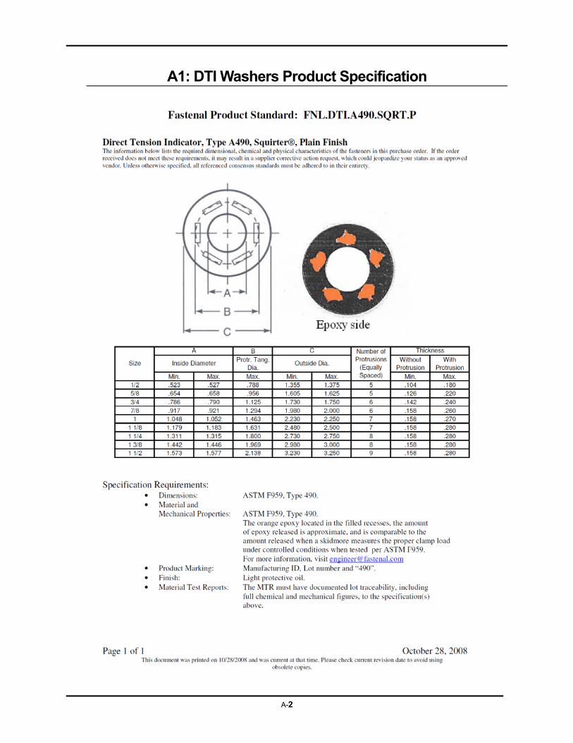
A-2

A1: DTI Washers Product Specification

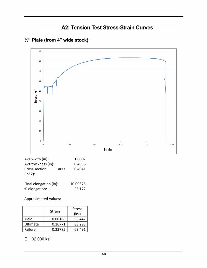
A-3

A2: Tension Test Stress-Strain Curves

½” Plate (from 4” wide stock)

Avg width (in): 1.0007Avg thickness (in): 0.4938Cross‐section area (in^2):

0.4941

Final elongation (in): 10.09375% elongation: 26.172

Approximated Values:

Strain

Stress (ksi)

Yield 0.00168 53.447

Ultimate 0.16771 83.293

Failure 0.23785 63.491 E ~ 32,000 ksi

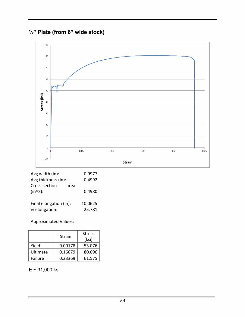
A-4

½” Plate (from 6” wide stock)

Avg width (in): 0.9977 Avg thickness (in): 0.4992 Cross‐section area (in^2): 0.4980

Final elongation (in): 10.0625 % elongation: 25.781

Approximated Values:

Strain Stress (ksi)

Yield 0.00178 53.076

Ultimate 0.16679 80.696

Failure 0.23369 61.575 E ~ 31,000 ksi

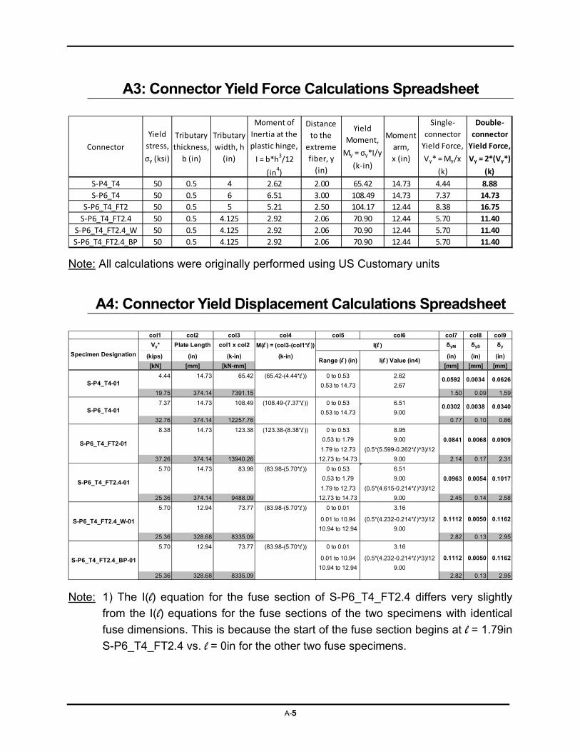
A-5

A3: Connector Yield Force Calculations Spreadsheet

Note: All calculations were originally performed using US Customary units

A4: Connector Yield Displacement Calculations Spreadsheet

Note: 1) The I(l) equation for the fuse section of S-P6_T4_FT2.4 differs very slightly

from the I(l) equations for the fuse sections of the two specimens with identical

fuse dimensions. This is because the start of the fuse section begins at l = 1.79in

S-P6_T4_FT2.4 vs. l = 0in for the other two fuse specimens.

Connector

Yield

stress,

σy (ksi)

Tributary

thickness,

b (in)

Tributary

width, h

(in)

Moment of

Inertia at the

plastic hinge,

I = b*h3/12

(in4)

Distance

to the

extreme

fiber, y

(in)

Yield

Moment,

My = σy*I/y

(k‐in)

Moment

arm,

x (in)

Single‐

connector

Yield Force,

Vy* = My/x

(k)

Double‐

connector

Yield Force,

Vy = 2*(Vy*)

(k)

S‐P4_T4 50 0.5 4 2.62 2.00 65.42 14.73 4.44 8.88

S‐P6_T4 50 0.5 6 6.51 3.00 108.49 14.73 7.37 14.73

S‐P6_T4_FT2 50 0.5 5 5.21 2.50 104.17 12.44 8.38 16.75

S‐P6_T4_FT2.4 50 0.5 4.125 2.92 2.06 70.90 12.44 5.70 11.40

S‐P6_T4_FT2.4_W 50 0.5 4.125 2.92 2.06 70.90 12.44 5.70 11.40

S‐P6_T4_FT2.4_BP 50 0.5 4.125 2.92 2.06 70.90 12.44 5.70 11.40

col1 col2 col3 col4 col5 col6 col7 col8 col9

Vy* Plate Length col1 x col2 M(l ) = (col3-(col1*l )) δyM δyS δy

(kips) (in) (k-in) (k-in) (in) (in) (in)

[kN] [mm] [kN-mm] [mm] [mm] [mm]

4.44 14.73 65.42 (65.42-(4.44*l )) 0 to 0.53 2.62

0.53 to 14.73 2.6719.75 374.14 7391.15 1.50 0.09 1.59

7.37 14.73 108.49 (108.49-(7.37*l )) 0 to 0.53 6.51

0.53 to 14.73 9.0032.76 374.14 12257.76 0.77 0.10 0.86

8.38 14.73 123.38 (123.38-(8.38*l )) 0 to 0.53 8.95

0.53 to 1.79 9.00 0.0841 0.0068 0.0909

1.79 to 12.73 (0.5*(5.599-0.262*l )^3)/12

37.26 374.14 13940.26 12.73 to 14.73 9.00 2.14 0.17 2.31

5.70 14.73 83.98 (83.98-(5.70*l )) 0 to 0.53 6.51

0.53 to 1.79 9.00 0.0963 0.0054 0.1017

1.79 to 12.73 (0.5*(4.615-0.214*l )^3)/12

25.36 374.14 9488.09 12.73 to 14.73 9.00 2.45 0.14 2.58

5.70 12.94 73.77 (83.98-(5.70*l )) 0 to 0.01 3.16

0.01 to 10.94 (0.5*(4.232-0.214*l )^3)/12 0.1112 0.0050 0.1162

10.94 to 12.94 9.0025.36 328.68 8335.09 2.82 0.13 2.95

5.70 12.94 73.77 (83.98-(5.70*l )) 0 to 0.01 3.16

0.01 to 10.94 (0.5*(4.232-0.214*l )^3)/12 0.1112 0.0050 0.1162

10.94 to 12.94 9.0025.36 328.68 8335.09 2.82 0.13 2.95

S-P6_T4_FT2.4_BP-01

S-P6_T4-01

S-P6_T4_FT2-01

S-P6_T4_FT2.4-01

S-P4_T4-01

S-P6_T4_FT2.4_W-01

Specimen Designation

I(l )

I(l ) Value (in4)Range (l ) (in)

0.0034

0.0038

0.0626

0.0340

0.0592

0.0302

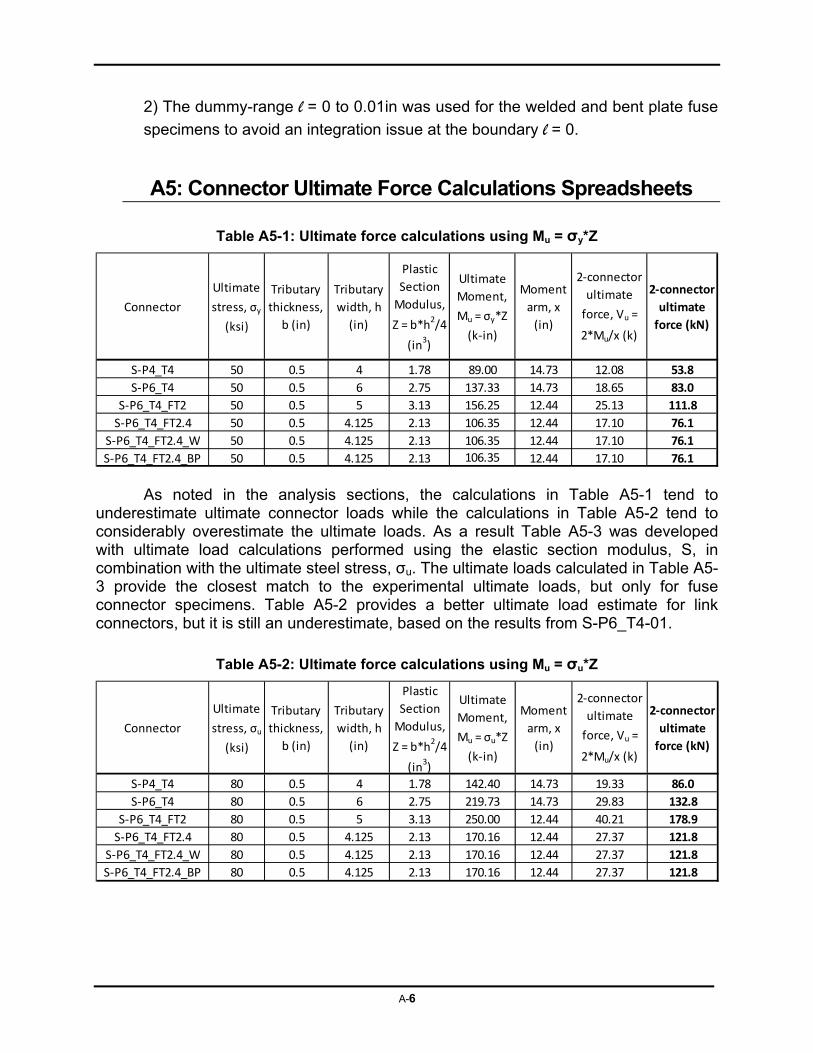
A-6

2) The dummy-range l = 0 to 0.01in was used for the welded and bent plate fuse

specimens to avoid an integration issue at the boundary l = 0.

A5: Connector Ultimate Force Calculations Spreadsheets

Table A5-1: Ultimate force calculations using Mu = σy*Z

As noted in the analysis sections, the calculations in Table A5-1 tend to underestimate ultimate connector loads while the calculations in Table A5-2 tend to considerably overestimate the ultimate loads. As a result Table A5-3 was developed with ultimate load calculations performed using the elastic section modulus, S, in combination with the ultimate steel stress, σu. The ultimate loads calculated in Table A5-3 provide the closest match to the experimental ultimate loads, but only for fuse connector specimens. Table A5-2 provides a better ultimate load estimate for link connectors, but it is still an underestimate, based on the results from S-P6_T4-01.

Table A5-2: Ultimate force calculations using Mu = σu*Z

Connector

Ultimate

stress, σy

(ksi)

Tributary

thickness,

b (in)

Tributary

width, h

(in)

Plastic

Section

Modulus,

Z = b*h2/4

(in3)

Ultimate

Moment,

Mu = σy*Z

(k‐in)

Moment

arm, x

(in)

2‐connector

ultimate

force, Vu =

2*Mu/x (k)

2‐connector

ultimate

force (kN)

S‐P4_T4 50 0.5 4 1.78 89.00 14.73 12.08 53.8

S‐P6_T4 50 0.5 6 2.75 137.33 14.73 18.65 83.0

S‐P6_T4_FT2 50 0.5 5 3.13 156.25 12.44 25.13 111.8

S‐P6_T4_FT2.4 50 0.5 4.125 2.13 106.35 12.44 17.10 76.1

S‐P6_T4_FT2.4_W 50 0.5 4.125 2.13 106.35 12.44 17.10 76.1

S‐P6_T4_FT2.4_BP 50 0.5 4.125 2.13 106.35 12.44 17.10 76.1

Connector

Ultimate

stress, σu

(ksi)

Tributary

thickness,

b (in)

Tributary

width, h

(in)

Plastic

Section

Modulus,

Z = b*h2/4

(in3)

Ultimate

Moment,

Mu = σu*Z

(k‐in)

Moment

arm, x

(in)

2‐connector

ultimate

force, Vu =

2*Mu/x (k)

2‐connector

ultimate

force (kN)

S‐P4_T4 80 0.5 4 1.78 142.40 14.73 19.33 86.0

S‐P6_T4 80 0.5 6 2.75 219.73 14.73 29.83 132.8

S‐P6_T4_FT2 80 0.5 5 3.13 250.00 12.44 40.21 178.9

S‐P6_T4_FT2.4 80 0.5 4.125 2.13 170.16 12.44 27.37 121.8

S‐P6_T4_FT2.4_W 80 0.5 4.125 2.13 170.16 12.44 27.37 121.8

S‐P6_T4_FT2.4_BP 80 0.5 4.125 2.13 170.16 12.44 27.37 121.8

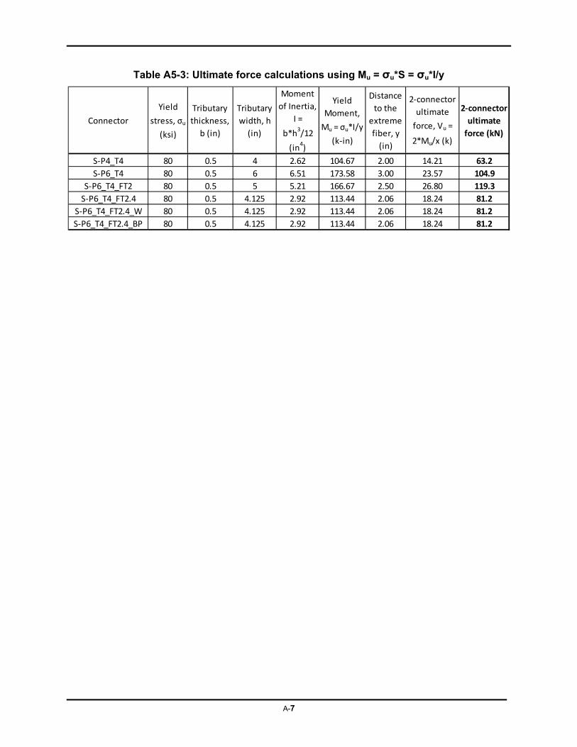
A-7

Table A5-3: Ultimate force calculations using Mu = σu*S = σu*I/y

Connector

Yield

stress, σu

(ksi)

Tributary

thickness,

b (in)

Tributary

width, h

(in)

Moment

of Inertia,

I =

b*h3/12

(in4)

Yield

Moment,

Mu = σu*I/y

(k‐in)

Distance

to the

extreme

fiber, y

(in)

2‐connector

ultimate

force, Vu =

2*Mu/x (k)

2‐connector

ultimate

force (kN)

S‐P4_T4 80 0.5 4 2.62 104.67 2.00 14.21 63.2

S‐P6_T4 80 0.5 6 6.51 173.58 3.00 23.57 104.9

S‐P6_T4_FT2 80 0.5 5 5.21 166.67 2.50 26.80 119.3

S‐P6_T4_FT2.4 80 0.5 4.125 2.92 113.44 2.06 18.24 81.2

S‐P6_T4_FT2.4_W 80 0.5 4.125 2.92 113.44 2.06 18.24 81.2

S‐P6_T4_FT2.4_BP 80 0.5 4.125 2.92 113.44 2.06 18.24 81.2

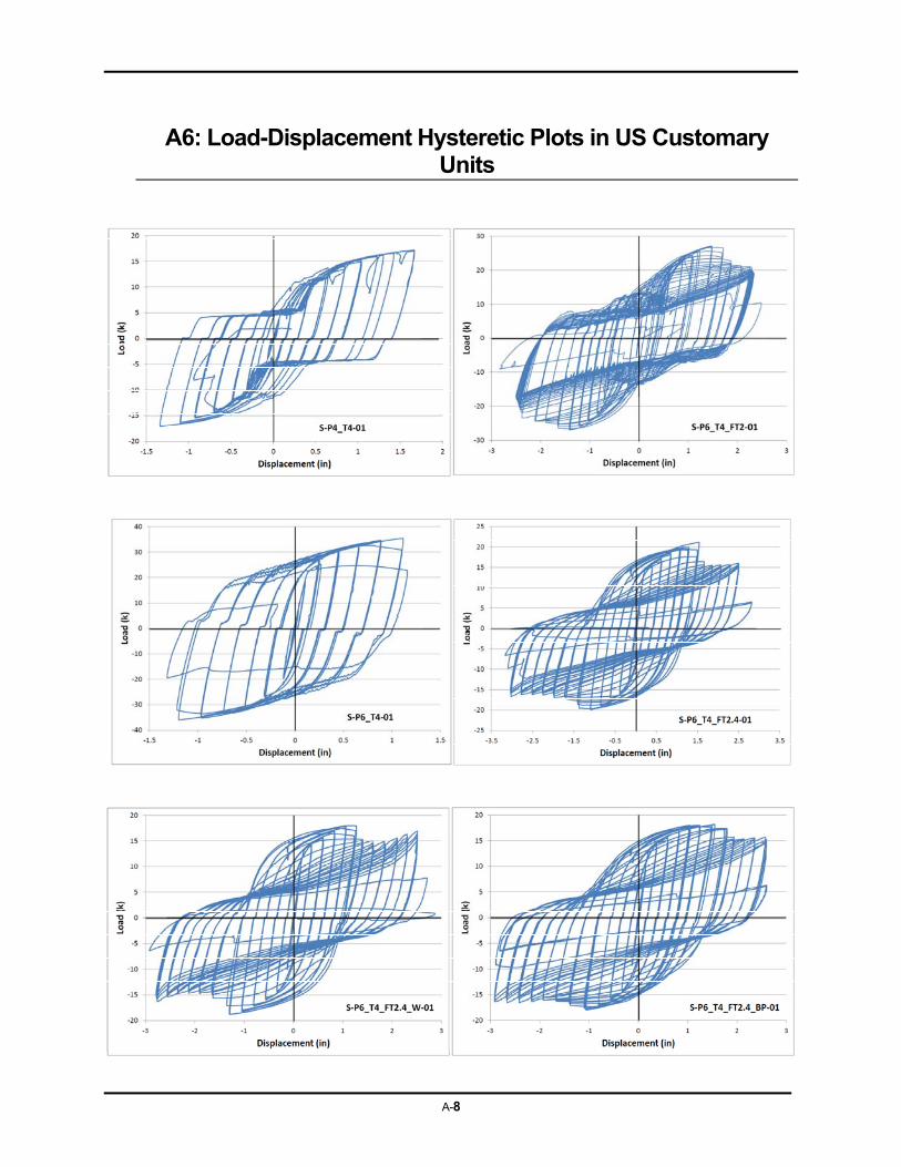
A-8

A6: Load-Displacement Hysteretic Plots in US Customary Units

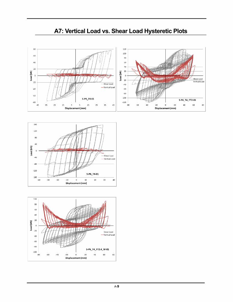
A-9

A7: Vertical Load vs. Shear Load Hysteretic Plots

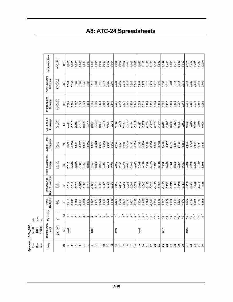
A-10

A8: ATC-24 Spreadsheets

Sp

ecim

enS

-P4

_T

4-0

1

Fy

=50

.00

ksi

Qy

=8

.88

kips

δy

=0

.06

26

in.

Ent

ryD

isp

lace

me

nt

Le

vel

Pe

ak

Def

lect

ion

De

flect

ion

at

Sta

rt o

f Exc

ursi

onP

last

ic D

efle

ctio

n R

ang

eL

oad

at P

ea

k D

efle

ctio

nM

ax.

Loa

d in

E

xcur

sio

nIn

itial

Lo

adi

ng

Stif

fne

ssIn

itia

l Unl

oad

ing

S

tiffn

ess

Hys

tere

sis

Are

a

(in.

) (+

/-)

i+i-

δ/δ

yδ

0/δ

yΔδ

pm/δ

yQ

/Qy

Qm

ax/Q

K0/

(Qy/δ

y)K

/(Q

y/δ

y)A

/(Qy*δ

y)

[1]

[2]

[4]

[5]

[6]

[7]

[8]

[9]

[10

][1

1]

10

.01

1+

0.1

12

0.01

30

.02

00

.00

90

.01

20

.08

00

.08

20.

000

21

--0

.04

00.

013

-0.0

26

-0.0

04-0

.01

80

.32

00

.09

10.

000

32

+0

.09

30.

020

-0.0

13

0.0

10

0.0

10

0.0

87

0.0

89

0.0

00

42

--0

.03

3-0

.013

0.0

00

-0.0

12-0

.01

80

.37

80

.38

90.

000

53

+0

.09

30.

000

0.0

53

0.0

06

0.0

09

0.0

70

0.0

45

0.0

00

63

--0

.02

70.

013

-0.0

13

-0.0

15-0

.01

70

.40

80

.53

70.

000

70

.02

4+

0.1

72

-0.0

070

.04

60

.02

60

.02

70

.00

50

.11

00.

000

84

--0

.07

30.

013

-0.0

20

-0.0

23-0

.04

50

.34

40

.23

10.

001

95

+0

.17

90.

020

-0.0

07

0.0

27

0.0

27

0.1

29

0.1

12

0.0

02

10

5-

-0.0

66

0.00

70

.00

0-0

.043

-0.0

43

0.3

60

0.3

76

0.0

03

11

6+

0.1

72

0.03

30

.01

30

.02

40

.02

80

.13

00

.12

00.

003

12

6-

-0.0

86

0.02

0-0

.04

60

.00

0-0

.04

20

.34

60

.00

10.

004

13

0.0

37

+0

.30

4-0

.027

0.1

59

0.1

00

0.1

12

0.0

04

0.3

28

0.0

08

14

7-

-0.2

05

0.11

2-0

.10

6-0

.107

-0.1

31

0.4

49

0.3

52

0.0

19

15

8+

0.3

24

0.05

30

.05

30

.04

80

.11

30

.32

40

.33

30.

005

16

8-

-0.2

32

0.08

6-0

.09

3-0

.125

-0.1

30

0.4

58

0.5

29

0.0

12

17

9+

0.3

37

0.00

70

.10

60

.11

00

.11

40

.37

50

.28

50.

017

18

9-

-0.2

32

0.07

3-0

.09

3-0

.129

-0.1

29

0.4

44

0.6

44

0.0

23

19

0.0

61

0+

0.6

09

-0.0

400

.09

30

.23

30

.23

70

.00

50

.85

70.

053

20

10

--0

.60

90.

040

-0.1

79

-0.2

76-0

.27

90

.51

40

.77

20.

100

21

11

+0

.59

5-0

.113

0.1

52

0.2

27

0.2

39

0.1

75

0.8

15

0.1

22

22

11

--0

.59

60.

020

-0.1

65

-0.2

66-0

.27

80

.45

20

.72

70.

161

23

12

+0

.61

5-0

.113

0.1

39

0.2

39

0.2

39

0.2

04

0.9

15

0.1

91

24

12

--0

.60

20.

000

-0.1

46

-0.2

78-0

.27

80

.46

90

.77

20.

234

25

0.1

01

3+

1.0

92

-0.1

260

.29

10

.41

20

.41

20

.00

10

.83

10.

342

26

13

--1

.07

20.

139

-0.4

10

-0.4

57-0

.45

70

.41

70

.81

60.

491

27

14

+1

.09

9-0

.245

0.3

51

0.4

20

0.4

20

0.1

26

0.7

94

0.5

98

28

14

--1

.06

50.

086

-0.3

90

-0.4

57-0

.45

70

.42

30

.84

40.

729

29

15

+1

.10

5-0

.278

0.3

57

0.4

18

0.4

25

0.0

97

0.7

44

0.8

36

30

15

--1

.07

20.

060

-0.3

37

-0.4

54-0

.46

00

.44

00

.87

30.

962

31

0.2

51

6+

3.2

96

-0.2

582

.50

10

.52

80

.55

20

.00

10

.74

42.

171

32

16

--3

.13

02.

230

-3.8

78

-0.7

93-0

.79

30

.15

60

.82

04.

316

33

17

+3

.28

9-1

.615

3.7

26

0.5

64

0.5

79

0.0

70

0.8

34

6.2

34

34

17

--3

.13

02.

078

-3.7

39

-0.7

87-0

.79

40

.16

10

.75

28.

280

35

18

+3

.28

2-1

.635

3.6

93

0.5

87

0.5

95

0.0

52

0.7

92

10

.20

1

Exc

ursi

on

[3]

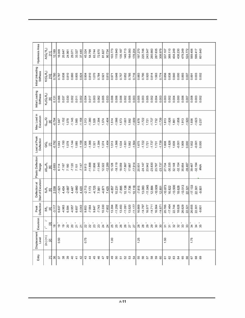
A-11

Ent

ryD

ispl

ace

me

nt

Le

vel

Pe

ak

De

flect

ion

De

flect

ion

at

Sta

rt o

f Exc

ursi

on

Pla

stic

De

flect

ion

Ra

nge

Lo

ad

at P

ea

k D

efle

ctio

nM

ax.

Lo

ad

in

Exc

ursi

on

Initi

al L

oa

din

g

Stif

fne

ssIn

itia

l Unl

oa

ding

S

tiffn

ess

Hys

tere

sis

Are

a

(in.

) (+

/-)i+

i-δ

/δy

δ0/δ

yΔδ p

m/δ

yQ

/Qy

Qm

ax/Q

K0/

(Qy/δ y

)K

/(Q

y/δ y

)A

/(Q

y*δ y

)

[1]

[2]

[4]

[5]

[6]

[7]

[8]

[9]

[10

][1

1]

36

18

--3

.117

2.03

8-3

.693

-0.7

92

-0.7

94

0.1

31

0.7

80

12.1

89

37

0.5

01

9+

6.6

37

-1.6

216

.11

41.

043

1.0

47

0.0

66

0.7

87

16.0

09

38

19

--4

.963

4.45

4-7

.167

-1.1

50

-1.1

52

0.0

37

0.8

38

20.6

47

39

20

+6

.58

4-2

.687

7.1

80

1.07

81

.07

80

.03

00

.81

024

.96

1

40

20

--4

.957

4.44

7-7

.120

-1.1

44

-1.1

45

0.0

02

0.8

60

29.0

71

41

21

+6

.65

7-2

.660

7.1

01

1.08

51

.08

50

.01

10

.80

533

.32

7

42

21

--5

.043

4.42

0-7

.147

-1.1

58

-1.1

58

0.0

02

0.8

24

37.4

40

43

0.7

52

2+

9.8

53

-2.7

139

.91

31.

308

1.3

13

0.0

04

0.9

04

45.3

24

44

22

--7

.564

7.17

3-1

1.8

98

-1.3

66

-1.3

80

0.0

17

0.8

10

54.7

99

45

23

+9

.84

7-4

.725

11.

806

1.32

11

.32

80

.00

31

.07

063

.74

4

46

23

--7

.743

7.06

1-1

1.9

45

-1.3

94

-1.3

94

0.0

62

0.7

84

72.6

70

47

24

+10

.33

0-4

.871

12.

322

1.37

41

.37

40

.00

50

.92

181

.82

7

48

24

--7

.802

7.42

5-1

2.2

89

-1.4

04

-1.4

04

0.0

33

0.8

10

90.7

34

49

1.0

02

5+

13.3

94

-4.8

571

5.12

81.

513

1.5

14

0.0

06

0.9

71

10

3.77

3

50

25

--1

1.2

56

10.2

31-1

8.1

19

-1.5

66

-1.5

66

0.0

06

0.6

48

11

9.94

0

51

26

+13

.49

3-7

.895

18.

059

1.53

41

.57

30

.00

60

.75

71

35.

187

52

26

--1

1.0

91

10.1

38-1

7.8

67

-1.6

01

-1.6

01

0.0

02

0.8

52

14

9.71

3

53

27

+13

.52

0-7

.736

17.

887

1.56

21

.59

20

.00

50

.78

51

64.

093

54

27

--1

1.1

77

10.1

18-1

7.9

14

-1.5

64

-1.6

09

0.0

03

0.7

16

17

8.20

4

55

1.2

52

8+

16.6

69

-7.8

152

0.93

11.

675

1.6

78

0.0

05

0.8

83

19

7.27

0

56

28

--1

4.7

97

13.0

83-2

4.1

47

-1.7

22

-1.7

22

0.0

03

0.7

90

22

0.74

6

57

29

+16

.57

7-1

1.04

52

3.94

21.

721

1.7

21

0.0

05

0.9

20

24

3.54

7

58

29

--1

4.7

11

12.8

84-2

3.8

30

-1.7

37

-1.7

37

0.0

02

0.8

14

26

5.66

0

59

30

+16

.56

4-1

0.93

92

3.79

71.

731

1.7

32

0.0

04

1.5

63

28

7.63

5

60

30

--1

4.6

71

12.8

51-2

3.7

37

-1.7

39

-1.7

39

0.0

03

0.7

74

30

8.97

9

61

1.5

03

1+

20.7

85

-10.

873

27.

734

1.80

81

.81

30

.00

30

.85

63

37.

107

62

31

--1

7.4

64

16.8

22-3

0.3

35

-1.8

26

-1.8

26

0.0

02

0.8

38

36

9.11

0

63

32

+22

.74

4-1

3.50

03

2.14

81.

839

1.8

61

0.0

04

0.8

40

40

4.24

9

64

32

-18

.62

818

.628

-32

.15

4-0

.00

1-1

.85

80

.00

00

.00

04

38.

230

65

33

+26

.62

9-1

3.51

33

5.85

41.

909

1.9

13

0.0

06

0.8

93

47

9.24

9

66

33

-22

.32

122

.321

-39

.48

70.

000

-1.9

20

0.0

07

0.0

07

52

4.77

2

67

1.7

53

4+

26.6

55

-17.

133

39.

467

1.93

21

.93

60

.00

80

.89

15

69.

406

68

34

-22

.30

122

.301

-32

.19

4-0

.00

1-1

.62

30

.00

30

.00

35

99.

417

69

35

+-9

.801

-9.8

01#

N/A

0.00

00

.23

70

.00

20

.00

26

01.

640

Exc

ursi

on

[3]

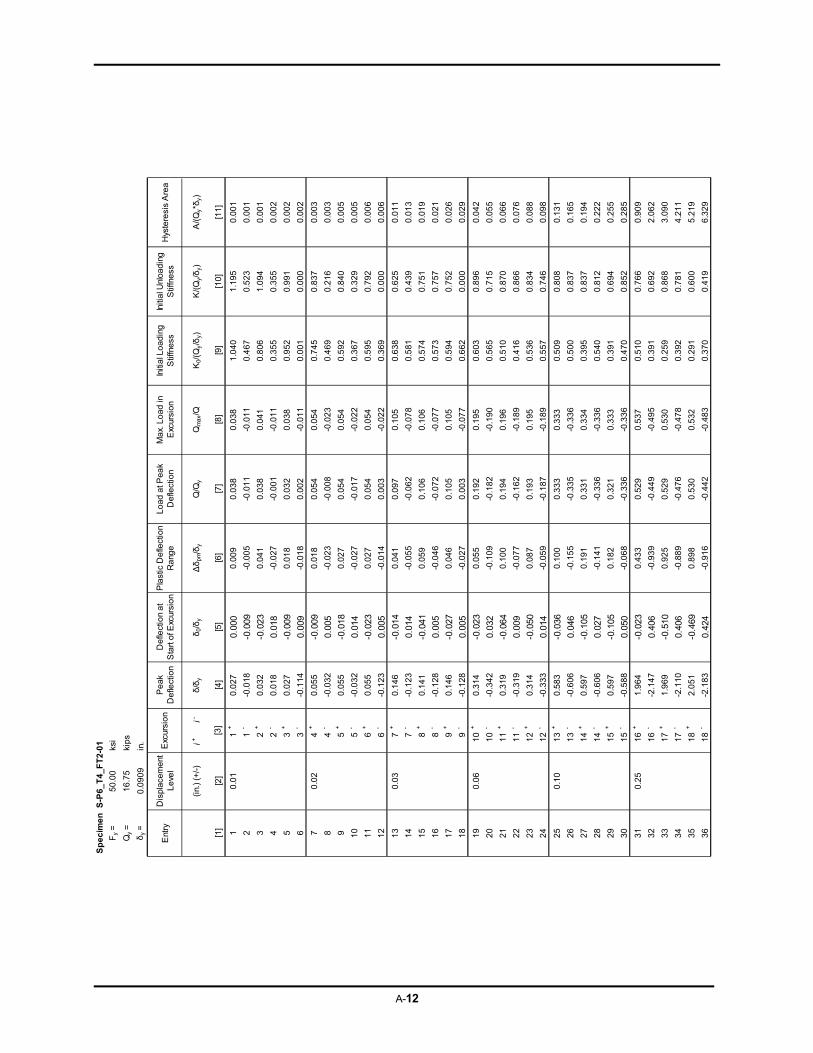
A-12

Sp

eci

me

nS

-P6_

T4_

FT

2-0

1

Fy

=5

0.0

0ks

i

Qy

=1

6.7

5ki

ps

δy

=0

.09

09

in.

Ent

ryD

isp

lace

me

nt

Le

vel

Pe

ak

Def

lect

ion

De

flect

ion

at

Sta

rt o

f Exc

ursi

on

Pla

stic

De

flect

ion

Ra

nge

Lo

ad

at P

ea

k D

efle

ctio

nM

ax.

Lo

ad

in

Exc

ursi

onIn

itia

l Lo

adin

g

Stif

fnes

sIn

itia

l Unl

oa

din

g

Stif

fnes

sH

yste

resi

s A

rea

(in.

) (+

/-)

i+i-

δ/δ

yδ

0/δ

yΔδ

pm/δ

yQ

/Qy

Qm

ax/Q

K0/

(Qy/δ

y)K

/(Q

y/δ

y)A

/(Q

y*δ

y)

[1]

[2]

[4]

[5]

[6]

[7]

[8]

[9]

[10

][1

1]

10

.01

1+

0.0

27

0.00

00

.00

90

.03

80

.03

81

.04

01

.19

50

.00

1

21

--0

.01

8-0

.009

-0.0

05

-0.0

11

-0.0

11

0.4

67

0.5

23

0.0

01

32

+0

.03

2-0

.023

0.0

41

0.0

38

0.0

41

0.8

06

1.0

94

0.0

01

42

-0

.01

80.

018

-0.0

27

-0.0

01

-0.0

11

0.3

55

0.3

55

0.0

02

53

+0

.02

7-0

.009

0.0

18

0.0

32

0.0

38

0.9

52

0.9

91

0.0

02

63

--0

.11

40.

009

-0.0

18

0.0

02

-0.0

11

0.0

01

0.0

00

0.0

02

70

.02

4+

0.0

55

-0.0

090

.01

80

.05

40

.05

40

.74

50

.83

70

.00

3

84

--0

.03

20.

005

-0.0

23

-0.0

08

-0.0

23

0.4

69

0.2

16

0.0

03

95

+0

.05

5-0

.018

0.0

27

0.0

54

0.0

54

0.5

92

0.8

40

0.0

05

10

5-

-0.0

32

0.01

4-0

.02

7-0

.01

7-0

.02

20

.36

70

.32

90

.00

5

11

6+

0.0

55

-0.0

230

.02

70

.05

40

.05

40

.59

50

.79

20

.00

6

12

6-

-0.1

23

0.00

5-0

.01

40

.00

3-0

.02

20

.36

90

.00

00

.00

6

13

0.0

37

+0

.14

6-0

.014

0.0

41

0.0

97

0.1

05

0.6

38

0.6

25

0.0

11

14

7-

-0.1

23

0.01

4-0

.05

5-0

.06

2-0

.07

80

.58

10

.43

90

.01

3

15

8+

0.1

41

-0.0

410

.05

90

.10

60

.10

60

.57

40

.75

10

.01

9

16

8-

-0.1

28

0.00

5-0

.04

6-0

.07

2-0

.07

70

.57

30

.75

70

.02

1

17

9+

0.1

46

-0.0

270

.04

60

.10

50

.10

50

.59

40

.75

20

.02

6

18

9-

-0.1

28

0.00

5-0

.02

70

.00

3-0

.07

70

.66

20

.00

00

.02

9

19

0.0

61

0+

0.3

14

-0.0

230

.05

50

.19

20

.19

50

.60

30

.89

60

.04

2

20

10

--0

.34

20.

032

-0.1

09

-0.1

82

-0.1

90

0.5

65

0.7

15

0.0

55

21

11

+0

.31

9-0

.064

0.1

00

0.1

94

0.1

96

0.5

10

0.8

70

0.0

66

22

11

--0

.31

90.

009

-0.0

77

-0.1

62

-0.1

89

0.4

16

0.8

66

0.0

76

23

12

+0

.31

4-0

.050

0.0

87

0.1

93

0.1

95

0.5

36

0.8

34

0.0

88

24

12

--0

.33

30.

014

-0.0

59

-0.1

87

-0.1

89

0.5

57

0.7

46

0.0

98

25

0.1

01

3+

0.5

83

-0.0

360

.10

00

.33

30

.33

30

.50

90

.80

80

.13

1

26

13

--0

.60

60.

046

-0.1

55

-0.3

35

-0.3

36

0.5

00

0.8

37

0.1

65

27

14

+0

.59

7-0

.105

0.1

91

0.3

31

0.3

34

0.3

95

0.8

37

0.1

94

28

14

--0

.60

60.

027

-0.1

41

-0.3

36

-0.3

36

0.5

40

0.8

12

0.2

22

29

15

+0

.59

7-0

.105

0.1

82

0.3

21

0.3

33

0.3

91

0.6

94

0.2

55

30

15

--0

.58

80.

050

-0.0

68

-0.3

36

-0.3

36

0.4

70

0.8

52

0.2

85

31

0.2

51

6+

1.9

64

-0.0

230

.43

30

.52

90

.53

70

.51

00

.76

60

.90

9

32

16

--2

.14

70.

406

-0.9

39

-0.4

49

-0.4

95

0.3

91

0.6

92

2.0

62

33

17

+1

.96

9-0

.510

0.9

25

0.5

29

0.5

30

0.2

59

0.8

68

3.0

90

34

17

--2

.11

00.

406

-0.8

89

-0.4

76

-0.4

78

0.3

92

0.7

81

4.2

11

35

18

+2

.05

1-0

.469

0.8

98

0.5

30

0.5

32

0.2

91

0.6

00

5.2

19

36

18

--2

.18

30.

424

-0.9

16

-0.4

42

-0.4

83

0.3

70

0.4

19

6.3

29

Exc

ursi

on

[3]

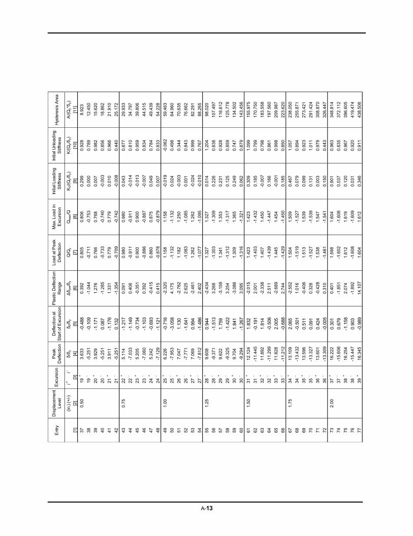
A-13

E

ntry

Dis

pla

cem

ent

L

eve

lP

ea

k D

efle

ctio

nD

efle

ctio

n a

t S

tart

of E

xcur

sio

nP

last

ic D

efle

ctio

n R

ang

eL

oa

d a

t Pe

ak

De

flect

ion

Ma

x. L

oa

d in

E

xcur

sio

nIn

itia

l Lo

ad

ing

S

tiffn

ess

Initi

al U

nlo

ad

ing

S

tiffn

ess

Hys

tere

sis

Are

a

(in.

) (+

/-)

i+i-

δ/δ

yδ

0/δ

yΔδ

pm/δ

yQ

/Qy

Qm

ax/Q

K0/

(Qy/δ

y)K

/(Q

y/δ

y)A

/(Q

y*δ

y)

[1]

[2]

[4]

[5]

[6]

[7]

[8]

[9]

[10

][1

1]

37

0.5

01

9+

3.6

33

-0.4

880

.39

20

.80

50

.80

60

.29

90

.92

88

.92

3

38

19

--5

.25

1-0

.109

-1.0

44

-0.7

11

-0.7

53

0.0

00

0.7

89

12

.45

0

39

20

+3

.92

9-1

.171

1.2

76

0.7

66

0.7

68

0.0

07

0.9

82

15

.62

0

40

20

--5

.25

10.

087

-1.2

85

-0.7

33

-0.7

40

-0.0

03

0.8

56

18

.86

2

41

21

+3

.91

1-1

.176

1.3

31

0.7

79

0.7

79

0.0

10

0.9

66

21

.91

0

42

21

--5

.25

10.

132

-1.3

54

-0.7

09

-0.7

42

-0.0

08

0.4

40

25

.17

2

43

0.7

52

2+

5.1

14

-1.2

170

.09

10

.98

00

.98

00

.04

30

.87

72

9.9

33

44

22

--7

.03

3-1

.149

0.4

06

-0.9

11

-0.9

11

-0.0

14

0.8

10

34

.79

7

45

23

+5

.20

5-0

.734

-0.3

51

0.9

00

0.9

00

-0.0

13

0.9

59

39

.80

6

46

23

--7

.06

0-1

.103

0.3

92

-0.8

86

-0.8

87

-0.0

07

0.8

34

44

.51

5

47

24

+5

.24

2-0

.693

-0.4

15

0.8

60

0.8

75

0.0

49

0.7

84

49

.43

9

48

24

--7

.12

9-1

.121

0.4

15

-0.8

78

-0.8

79

0.0

07

0.8

33

54

.22

8

49

1.0

02

5+

6.2

26

-0.7

16-2

.32

01

.15

81

.15

8-0

.01

9-0

.06

25

9.4

63

50

25

--7

.95

3-3

.058

4.1

75

-1.1

32

-1.1

32

0.0

24

0.4

98

64

.96

0

51

26

+7

.04

71.

130

-2.7

62

1.1

82

1.2

50

-0.0

03

0.3

44

70

.63

5

52

26

--7

.77

1-1

.641

2.6

25

-1.0

83

-1.0

85

0.0

01

0.8

43

76

.66

2

53

27

+7

.06

90.

994

-2.4

61

1.2

62

1.2

62

-0.0

24

0.9

99

82

.29

1

54

27

--7

.81

2-1

.486

2.4

02

-1.0

77

-1.0

95

-0.0

10

0.7

67

88

.26

5

55

1.2

52

8+

9.6

08

0.94

4-2

.43

41

.32

71

.32

70

.01

41

.20

49

8.0

20

56

28

--9

.37

1-1

.513

3.2

68

-1.3

03

-1.3

09

0.2

26

0.8

38

10

7.4

97

57

29

+9

.62

21.

759

-3.1

59

1.3

41

1.3

53

0.2

31

0.9

28

11

6.6

12

58

29

--9

.32

5-1

.422

3.2

54

-1.3

12

-1.3

17

0.1

25

0.8

59

12

5.7

78

59

30

+9

.70

41.

841

-3.0

86

1.3

09

1.3

65

0.2

49

0.7

47

13

4.5

02

60

30

--9

.29

4-1

.267

3.0

95

-1.3

16

-1.3

21

0.0

62

0.8

79

14

3.4

56

61

1.5

03

1+

12

.12

41.

832

-2.0

15

1.4

23

1.4

23

0.3

09

1.0

99

15

5.9

75

62

31

--1

1.4

45

-0.1

912

.00

1-1

.40

3-1

.43

20

.18

50

.79

91

70

.75

0

63

32

+1

1.8

92

1.81

4-2

.33

81

.40

71

.45

0-0

.00

70

.79

81

83

.55

8

64

32

--1

1.2

99

-0.5

062

.51

1-1

.43

9-1

.44

70

.16

60

.86

11

97

.56

0

65

33

+1

1.8

28

2.00

5-2

.68

91

.44

51

.45

4-0

.00

10

.99

82

09

.98

7

66

33

--1

1.2

12

-0.6

882

.74

4-1

.42

9-1

.45

00

.18

50

.85

02

23

.62

0

67

1.7

53

4+

13

.10

92.

065

-2.5

52

1.5

04

1.5

09

0.4

67

1.0

57

23

8.0

50

68

34

--1

3.4

32

-0.5

011

.01

6-1

.51

9-1

.52

70

.07

90

.89

42

55

.87

1

69

35

+1

3.5

96

0.51

1-0

.40

61

.51

31

.53

90

.09

90

.92

32

73

.42

1

70

35

--1

3.3

27

0.09

10

.32

8-1

.52

7-1

.53

90

.13

11

.01

12

91

.42

4

71

36

+1

3.6

01

0.42

4-0

.42

81

.53

81

.54

70

.00

30

.97

93

08

.87

0

72

36

--1

3.3

09

-0.0

050

.31

0-1

.46

1-1

.54

10

.15

00

.44

33

26

.44

7

73

2.0

03

7+

16

.22

20.

301

0.4

01

1.5

98

1.6

04

0.9

01

0.9

63

34

8.8

14

74

37

--1

5.6

06

0.67

9-1

.85

1-1

.60

2-1

.60

80

.03

70

.83

53

72

.11

2

75

38

+1

6.2

54

-1.1

582

.07

41

.61

21

.61

90

.12

00

.96

73

96

.60

5

76

38

--1

5.4

47

0.90

3-1

.89

2-1

.60

8-1

.60

90

.03

10

.92

04

19

.47

4

77

39

+1

6.3

45

-0.9

891

4.1

07

1.6

04

1.6

12

0.3

46

0.9

11

43

8.5

06

Exc

ursi

on

[3]

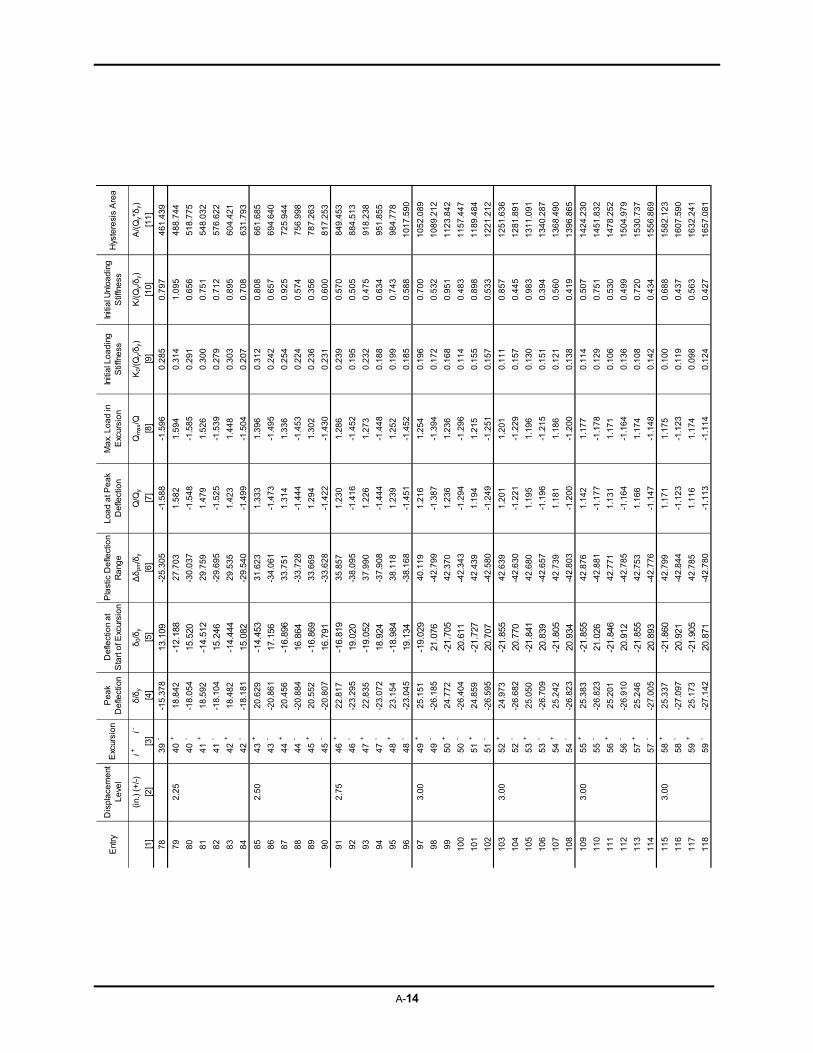
A-14

Ent

ryD

isp

lace

me

nt

Le

vel

Pe

ak

De

flect

ion

De

flect

ion

at

Sta

rt o

f Exc

ursi

on

Pla

stic

De

flect

ion

Ra

nge

Loa

d a

t Pe

ak

De

flect

ion

Ma

x. L

oa

d in

E

xcur

sio

nIn

itia

l Lo

ad

ing

S

tiffn

ess

Initi

al U

nlo

adi

ng

Stif

fne

ssH

yste

resi

s A

rea

(in.)

(+/-

)i+

i-δ

/δy

δ 0/δ

yΔδ

pm/δ

yQ

/Qy

Qm

ax/Q

K0/

(Qy/δ

y)K

/(Q

y/δ

y)A

/(Q

y*δ

y)

[1]

[2]

[4]

[5]

[6]

[7]

[8]

[9]

[10

][1

1]

78

39

--1

5.37

813

.109

-25.

30

5-1

.58

8-1

.59

60

.28

50

.79

74

61

.439

79

2.2

54

0+

18

.84

2-1

2.18

82

7.7

03

1.5

82

1.5

94

0.3

14

1.0

95

48

8.7

44

80

40

--1

8.05

415

.520

-30.

03

7-1

.54

8-1

.58

50

.29

10

.65

65

18

.775

81

41

+1

8.5

92

-14.

512

29

.75

91

.47

91

.52

60

.30

00

.75

15

48

.032

82

41

--1

8.10

415

.246

-29.

69

5-1

.52

5-1

.53

90

.27

90

.71

25

76

.622

83

42

+1

8.4

82

-14.

444

29

.53

51

.42

31

.44

80

.30

30

.89

56

04

.421

84

42

--1

8.18

115

.082

-29.

54

0-1

.49

9-1

.50

40

.20

70

.70

86

31

.793

85

2.5

04

3+

20

.62

9-1

4.45

33

1.6

23

1.3

33

1.3

96

0.3

12

0.8

08

66

1.6

85

86

43

--2

0.86

117

.156

-34.

06

1-1

.47

3-1

.49

50

.24

20

.65

76

94

.640

87

44

+2

0.4

56

-16.

896

33

.75

11

.31

41

.33

60

.25

40

.92

57

25

.944

88

44

--2

0.88

416

.864

-33.

72

8-1

.44

4-1

.45

30

.22

40

.57

47

56

.998

89

45

+2

0.5

52

-16.

869

33

.66

91

.29

41

.30

20

.23

60

.35

67

87

.263

90

45

--2

0.80

716

.791

-33.

62

8-1

.42

2-1

.43

00

.23

10

.60

08

17

.253

91

2.7

54

6+

22

.81

7-1

6.81

93

5.8

57

1.2

30

1.2

86

0.2

39

0.5

70

84

9.4

53

92

46

--2

3.29

519

.020

-38.

09

5-1

.41

6-1

.45

20

.19

50

.50

58

84

.513

93

47

+2

2.8

35

-19.

052

37

.99

01

.22

61

.27

30

.23

20

.47

59

18

.238

94

47

--2

3.07

218

.924

-37.

90

8-1

.44

4-1

.44

80

.18

80

.63

49

51

.855

95

48

+2

3.1

54

-18.

984

38

.11

81

.23

91

.25

20

.19

90

.74

39

84

.778

96

48

--2

3.04

519

.134

-38.

16

8-1

.45

1-1

.45

20

.18

50

.58

81

01

7.5

90

97

3.0

04

9+

25

.15

1-1

9.02

94

0.1

19

1.2

16

1.2

54

0.1

96

0.7

00

10

52

.08

9

98

49

--2

6.18

521

.076

-42.

79

9-1

.38

7-1

.39

40

.17

20

.53

21

08

9.2

12

99

50

+2

4.7

72

-21.

705

42

.37

01

.23

61

.23

60

.16

80

.95

11

12

3.8

42

10

05

0-

-26.

404

20.6

11-4

2.3

43

-1.2

94

-1.2

96

0.1

14

0.4

83

11

57

.44

7

10

15

1+

24

.85

9-2

1.72

74

2.4

39

1.1

94

1.2

15

0.1

55

0.8

98

11

89

.48

4

10

25

1-

-26.

595

20.7

07-4

2.5

80

-1.2

49

-1.2

51

0.1

57

0.5

33

12

21

.21

2

10

33

.00

52

+2

4.9

73

-21.

855

42

.63

91

.20

11

.20

10

.11

10

.85

71

25

1.6

36

10

45

2-

-26.

682

20.7

70-4

2.6

30

-1.2

21

-1.2

29

0.1

57

0.4

45

12

81

.89

1

10

55

3+

25

.05

0-2

1.84

14

2.6

80

1.1

95

1.1

96

0.1

30

0.9

83

13

11

.09

1

10

65

3-

-26.

709

20.8

39-4

2.6

57

-1.1

96

-1.2

15

0.1

51

0.3

94

13

40

.28

7

10

75

4+

25

.24

2-2

1.80

54

2.7

39

1.1

81

1.1

86

0.1

21

0.5

60

13

68

.49

0

10

85

4-

-26.

823

20.9

34-4

2.8

03

-1.2

00

-1.2

00

0.1

38

0.4

19

13

96

.86

5

10

93

.00

55

+2

5.3

83

-21.

855

42

.87

61

.14

21

.17

70

.11

40

.50

71

42

4.2

30

11

05

5-

-26.

823

21.0

26-4

2.8

81

-1.1

77

-1.1

78

0.1

29

0.7

51

14

51

.83

2

11

15

6+

25

.20

1-2

1.84

64

2.7

71

1.1

31

1.1

71

0.1

06

0.5

30

14

78

.25

2

11

25

6-

-26.

910

20.9

12-4

2.7

85

-1.1

64

-1.1

64

0.1

36

0.4

99

15

04

.97

9

11

35

7+

25

.24

6-2

1.85

54

2.7

53

1.1

66

1.1

74

0.1

08

0.7

20

15

30

.73

7

11

45

7-

-27.

005

20.8

93-4

2.7

76

-1.1

47

-1.1

48

0.1

42

0.4

34

15

56

.86

9

11

53

.00

58

+2

5.3

37

-21.

860

42

.79

91

.17

11

.17

50

.10

00

.68

81

58

2.1

23

11

65

8-

-27.

097

20.9

21-4

2.8

44

-1.1

23

-1.1

23

0.1

19

0.4

37

16

07

.59

0

11

75

9+

25

.17

3-2

1.90

54

2.7

85

1.1

16

1.1

74

0.0

98

0.5

63

16

32

.24

1

11

85

9-

-27.

142

20.8

71-4

2.7

80

-1.1

13

-1.1

14

0.1

24

0.4

27

16

57

.08

1

[3]

Exc

ursi

on

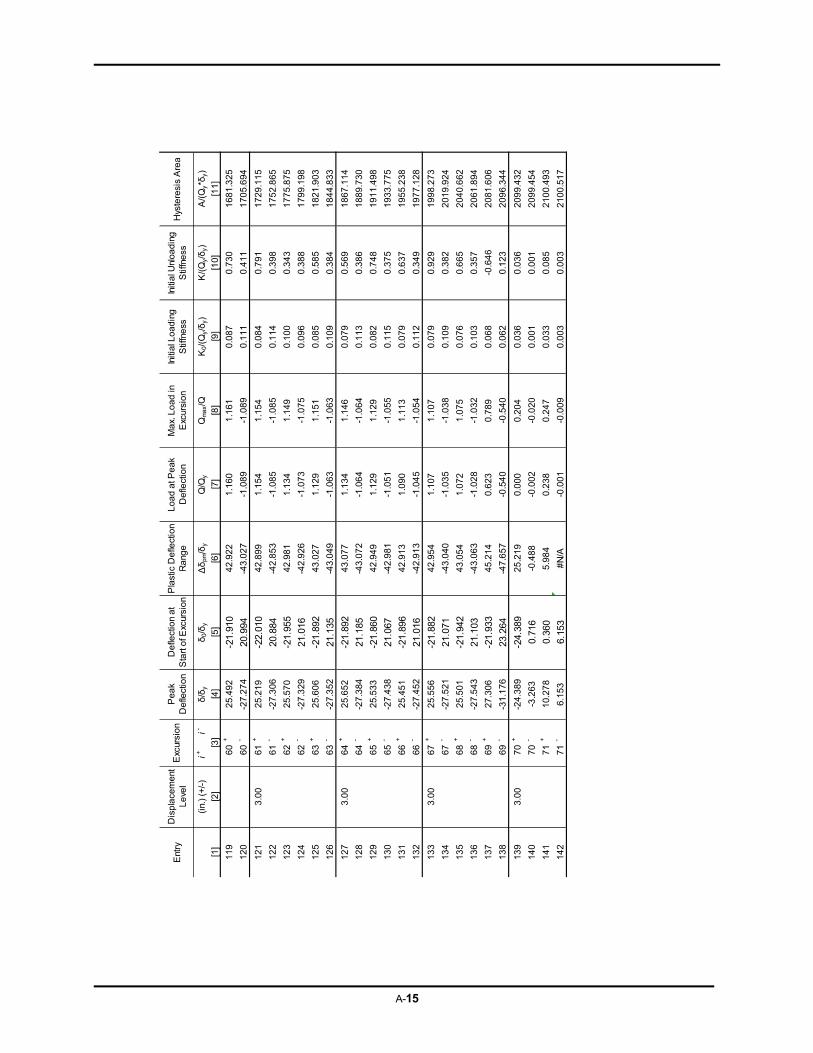
A-15

Ent

ryD

isp

lace

me

nt

Le

vel

Pea

k D

efle

ctio

nD

efle

ctio

n a

t S

tart

of E

xcur

sion

Pla

stic

De

flect

ion

Ran

ge

Loa

d a

t Pe

ak

De

flect

ion

Ma

x. L

oad

in

Exc

ursi

onIn

itial

Lo

adin

g

Stif

fne

ssIn

itial

Unl

oad

ing

Stif

fne

ssH

yste

resi

s A

rea

(in.

) (+

/-)

i+i-

δ/δ

yδ

0/δ

yΔδ

pm/δ

yQ

/Qy

Qm

ax/Q

K0/

(Qy/δ y

)K

/(Q

y/δ y

)A

/(Q

y*δ

y)

[1]

[2]

[4]

[5]

[6]

[7]

[8]

[9]

[10]

[11

]

119

60+

25.4

92

-21.

910

42.9

22

1.1

601

.16

10.

087

0.7

30

168

1.3

25

120

60-

-27.

274

20.9

94-4

3.0

27-1

.08

9-1

.089

0.1

110

.41

11

705.

694

121

3.0

061

+25

.21

9-2

2.01

042

.89

91.

154

1.1

54

0.0

840

.79

11

729.

115

122

61-

-27.

306

20.8

84-4

2.8

53-1

.08

5-1

.085

0.1

140

.39

81

752.

865

123

62+

25.5

70

-21.

955

42.9

81

1.1

341

.14

90.

100

0.3

43

177

5.8

75

124

62-

-27.

329

21.0

16-4

2.9

26-1

.07

3-1

.075

0.0

960

.38

81

799.

198

125

63+

25.6

06

-21.

892

43.0

27

1.1

291

.15

10.

085

0.5

85

182

1.9

03

126

63-

-27.

352

21.1

35-4

3.0

49-1

.06

3-1

.063

0.1

090

.38

41

844.

833

127

3.0

064

+25

.65

2-2

1.89

243

.07

71.

134

1.1

46

0.0

790

.56

91

867.

114

128

64-

-27.

384

21.1

85-4

3.0

72-1

.06

4-1

.064

0.1

130

.38

61

889.

730

129

65+

25.5

33

-21.

860

42.9

49

1.1

291

.12

90.

082

0.7

48

191

1.4

98

130

65-

-27.

438

21.0

67-4

2.9

81-1

.05

1-1

.055

0.1

150

.37

51

933.

775

131

66+

25.4

51

-21.

896

42.9

13

1.0

901

.11

30.

079

0.6

37

195

5.2

38

132

66-

-27.

452

21.0

16-4

2.9

13-1

.04

5-1

.054

0.1

120

.34

91

977.

128

133

3.0

067

+25

.55

6-2

1.88

242

.95

41.

107

1.1

07

0.0

790

.92

91

998.

273

134

67-

-27.

521

21.0

71-4

3.0

40-1

.03

5-1

.038

0.1

090

.38

22

019.

924

135

68+

25.5

01

-21.

942

43.0

54

1.0

721

.07

50.

076

0.6

65

204

0.6

62

136

68-

-27.

543

21.1

03-4

3.0

63-1

.02

8-1

.032

0.1

030

.35

72

061.

894

137

69+

27.3

06

-21.

933

45.2

14

0.6

230

.78

90.

068

-0.6

46

208

1.6

06

138

69-

-31.

176

23.2

64-4

7.6

57-0

.54

0-0

.540

0.0

620

.12

32

096.

344

139

3.0

070

+-2

4.3

89-2

4.38

925

.21

90.

000

0.2

04

0.0

360

.03

62

099.

432

140

70-

-3.2

63

0.71

6-0

.48

8-0

.00

2-0

.020

0.0

010

.00

12

099.

454

141

71+

10.2

78

0.36

05

.98

40.

238

0.2

47

0.0

330

.08

52

100.

493

142

71-

6.1

53

6.15

3#

N/A

-0.0

01

-0.0

090.

003

0.0

03

210

0.5

17

Exc

ursi

on

[3]

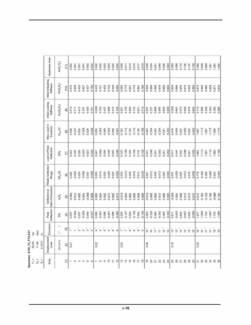
A-16

S

pe

cim

en

S-P

6_

T4

_F

T2

.4-0

1

Fy

=5

0.0

0ks

i

Qy

=1

1.4

0ki

ps

δy

=0

.10

17

in.

Ent

ryD

isp

lace

me

nt

Le

vel

Pe

ak

De

flect

ion

De

flect

ion

at

Sta

rt o

f Exc

ursi

on

Pla

stic

De

flect

ion

Ra

nge

Lo

ad

at P

ea

k D

efle

ctio

nM

ax.

Lo

ad

in

Exc

ursi

on

Initi

al L

oa

din

g

Stif

fne

ssIn

itia

l Unl

oa

din

g

Stif

fne

ssH

yste

resi

s A

rea

(in.

) (+

/-)

i+i-

δ/δ

yδ

0/δ

yΔδ

pm/δ

yQ

/Qy

Qm

ax/Q

K0/

(Qy/δ

y)K

/(Q

y/δ

y)A

/(Q

y*δ

y)

[1]

[2]

[4]

[5]

[6]

[7]

[8]

[9]

[10

][1

1]

10

.01

1+

0.0

57

-0.0

040

.02

00

.02

40

.02

80

.41

30

.41

00

.00

0

21

--0

.02

90.

012

-0.0

20

-0.0

27

-0.0

27

0.7

11

0.8

39

0.0

01

32

+0

.05

70.

000

0.0

24

0.0

26

0.0

26

0.4

13

0.4

25

0.0

01

42

--0

.02

90.

004

-0.0

08

-0.0

23

-0.0

28

0.7

91

0.8

27

0.0

01

53

+0

.04

9-0

.008

0.0

33

0.0

23

0.0

26

0.4

20

0.4

37

0.0

02

63

--0

.03

70.

008

-0.0

08

-0.0

24

-0.0

28

0.7

01

0.7

56

0.0

02

70

.02

4+

0.0

90

0.00

00

.02

00

.04

70

.05

0-0

.02

80

.43

50

.00

2

84

--0

.06

10.

004

-0.0

12

-0.0

50

-0.0

52

0.7

52

0.7

01

0.0

02

95

+0

.09

80.

000

0.0

29

0.0

46

0.0

49

0.4

37

0.4

02

0.0

03

10

5-

-0.0

61

0.01

2-0

.02

9-0

.04

0-0

.05

20

.68

80

.74

20

.00

3

11

6+

0.0

98

0.00

00

.02

40

.04

50

.04

80

.41

40

.42

90

.00

4

12

6-

-0.0

65

0.01

2-0

.02

9-0

.04

9-0

.05

10

.72

00

.69

40

.00

4

13

0.0

37

+0

.20

4-0

.012

0.0

33

0.1

20

0.1

20

0.0

01

0.5

84

0.0

08

14

7-

-0.1

47

0.00

4-0

.01

2-0

.10

9-0

.11

20

.73

50

.77

50

.01

1

15

8+

0.2

04

0.00

00

.02

90

.12

00

.12

00

.60

00

.60

10

.01

3

16

8-

-0.1

39

0.00

8-0

.01

6-0

.10

6-0

.11

00

.73

30

.77

90

.01

5

17

9+

0.2

04

0.00

80

.01

20

.11

60

.12

00

.62

10

.66

10

.01

7

18

9-

-0.1

39

0.00

8-0

.01

6-0

.10

5-0

.10

80

.71

00

.79

90

.01

9

19

0.0

61

0+

0.3

63

-0.0

120

.04

10

.24

10

.24

20

.02

70

.92

90

.02

8

20

10

--0

.33

40.

008

-0.0

12

-0.2

46

-0.2

54

0.7

27

0.8

96

0.0

34

21

11

+0

.36

30.

008

0.0

29

0.2

41

0.2

42

0.6

08

0.8

90

0.0

41

22

11

--0

.34

20.

012

-0.0

12

-0.2

52

-0.2

54

0.6

94

0.8

78

0.0

49

23

12

+0

.36

30.

008

0.0

20

0.2

41

0.2

41

0.6

06

0.8

99

0.0

56

24

12

--0

.34

20.

020

-0.0

24

-0.2

52

-0.2

53

0.6

59

0.8

54

0.0

63

25

0.1

01

3+

0.6

11

-0.0

040

.03

70

.41

70

.41

9-0

.00

50

.80

90

.08

3

26

13

--0

.60

30.

024

-0.0

29

-0.4

41

-0.4

54

0.6

61

0.8

96

0.0

99

27

14

+0

.62

40.

008

0.0

20

0.4

22

0.4

22

0.5

73

0.8

50

0.1

15

28

14

--0

.60

70.

012

-0.0

12

-0.4

46

-0.4

52

0.6

46

0.8

15

0.1

26

29

15

+0

.62

40.

012

0.0

16

0.4

21

0.4

22

0.5

78

0.8

22

0.1

37

30

15

--0

.59

90.

012

-0.0

08

-0.4

52

-0.4

52

0.6

54

0.8

64

0.1

48

31

0.2

51

6+

1.6

71

0.01

20

.17

91

.06

31

.06

70

.11

00

.87

40

.36

0

32

16

--1

.60

90.

183

-0.3

26

-1.1

13

-1.1

13

0.5

89

0.8

49

0.6

39

33

17

+1

.72

4-0

.122

0.3

06

1.0

87

1.0

87

0.3

48

0.8

80

0.8

60

34

17

--1

.59

70.

159

-0.2

69

-1.1

10

-1.1

12

0.5

23

0.8

26

1.0

81

35

18

+1

.72

4-0

.086

0.2

44

1.0

86

1.0

89

0.3

92

0.8

71

1.2

84

36

18

--1

.58

50.

130

-0.2

44

-1.1

06

-1.1

10

0.5

86

0.8

32

1.4

82

Exc

ursi

on

[3]

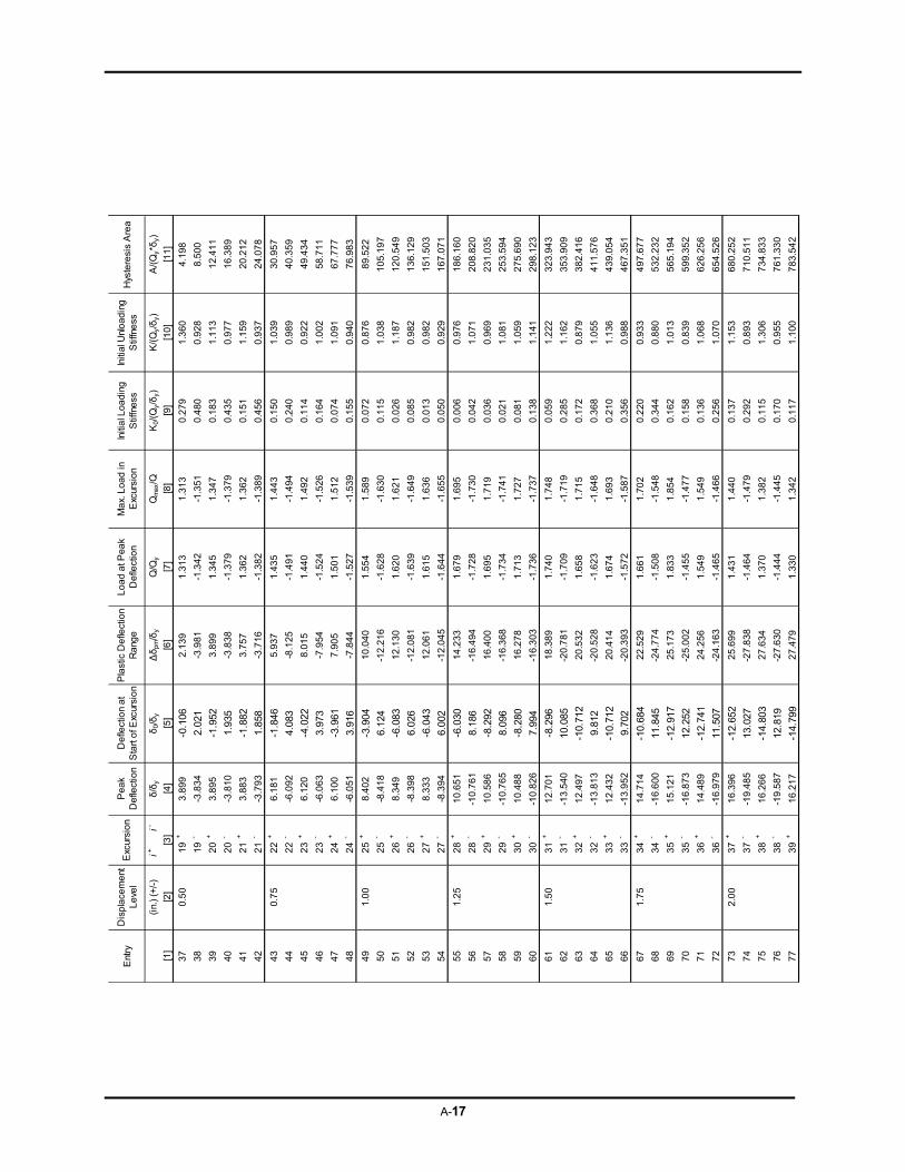
A-17

E

ntry

Dis

pla

cem

ent

L

eve

lP

ea

k D

efle

ctio

nD

efle

ctio

n a

t S

tart

of E

xcur

sio

nP

last

ic D

efle

ctio

n R

ang

eL

oa

d a

t Pe

ak

De

flect

ion

Ma

x. L

oa

d in

E

xcur

sio

nIn

itia

l Lo

ad

ing

S

tiffn

ess

Initi

al U

nlo

ad

ing

S

tiffn

ess

Hys

tere

sis

Are

a

(in.

) (+

/-)

i+i-

δ/δ

yδ

0/δ

yΔδ

pm/δ

yQ

/Qy

Qm

ax/Q

K0/

(Qy/δ

y)K

/(Q

y/δ

y)A

/(Q

y*δ

y)

[1]

[2]

[4]

[5]

[6]

[7]

[8]

[9]

[10

][1

1]

37

0.5

01

9+

3.8

99

-0.1

062

.13

91

.31

31

.31

30

.27

91

.36

04

.19

8

38

19

--3

.83

42.

021

-3.9

81

-1.3

42

-1.3

51

0.4

80

0.9

28

8.5

00

39

20

+3

.89

5-1

.952

3.8

99

1.3

45

1.3

47

0.1

83

1.1

13

12

.41

1

40

20

--3

.81

01.

935

-3.8

38

-1.3

79

-1.3

79

0.4

35

0.9

77

16

.38

9

41

21

+3

.88

3-1

.882

3.7

57

1.3

62

1.3

62

0.1

51

1.1

59

20

.21

2

42

21

--3

.79

31.

858

-3.7

16

-1.3

82

-1.3

89

0.4

56

0.9

37

24

.07

8

43

0.7

52

2+

6.1

81

-1.8

465

.93

71

.43

51

.44

30

.15

01

.03

93

0.9

57

44

22

--6

.09

24.

083

-8.1

25

-1.4

91

-1.4

94

0.2

40

0.9

89

40

.35

9

45

23

+6

.12

0-4

.022

8.0

15

1.4

40

1.4

92

0.1

14

0.9

22

49

.43

4

46

23

--6

.06

33.

973

-7.9

54

-1.5

24

-1.5

26

0.1

64

1.0

02

58

.71

1

47

24

+6

.10

0-3

.961

7.9

05

1.5

01

1.5

12

0.0

74

1.0

91

67

.77

7

48

24

--6

.05

13.

916

-7.8

44

-1.5

27

-1.5

39

0.1

55

0.9

40

76

.98

3

49

1.0

02

5+

8.4

02

-3.9

041

0.0

40

1.5

54

1.5

89

0.0

72

0.8

76

89

.52

2

50

25

--8

.41

86.

124

-12

.21

6-1

.62

8-1

.63

00

.11

51

.03

81

05

.19

7

51

26

+8

.34

9-6

.083

12

.13

01

.62

01

.62

10

.02

61

.18

71

20

.54

9

52

26

--8

.39

86.

026

-12

.08

1-1

.63

9-1

.64

90

.08

50

.98

21

36

.12

9

53

27

+8

.33

3-6

.043

12

.06

11

.61

51

.63

60

.01

30

.98

21

51

.50

3

54

27

--8

.39

46.

002

-12

.04

5-1

.64

4-1

.65

50

.05

00

.92

91

67

.07

1

55

1.2

52

8+

10

.65

1-6

.030

14

.23

31

.67

91

.69

50

.00

60

.97

61

86

.16

0

56

28

--1

0.7

61

8.18

6-1

6.4

94

-1.7

28

-1.7

30

0.0

42

1.0

71

20

8.8

20

57

29

+1

0.5

86

-8.2

921

6.4

00

1.6

95

1.7

19

0.0

36

0.9

69

23

1.0

35

58

29

--1

0.7

65

8.09

6-1

6.3

68

-1.7

34

-1.7

41

0.0

21

1.0

81

25

3.5

94

59

30

+1

0.4

88

-8.2

801

6.2

78

1.7

13

1.7

27

0.0

81

1.0

59

27

5.6

90

60

30

--1

0.8

26

7.99

4-1

6.3

03

-1.7

36

-1.7

37

0.1

38

1.1

41

29

8.1

23

61

1.5

03

1+

12

.70

1-8

.296

18

.38

91

.74

01

.74

80

.05

91

.22

23

23

.94

3

62

31

--1

3.5

40

10.0

85-2

0.7

81

-1.7

09

-1.7

19

0.2

85

1.1

62

35

3.9

09

63

32

+1

2.4

97

-10.

712

20

.53

21

.65

81

.71

50

.17

20

.87

93

82

.41

6

64

32

--1

3.8

13

9.81

2-2

0.5

28

-1.6

23

-1.6

48

0.3

68

1.0

55

41

1.5

76

65

33

+1

2.4

32

-10.

712

20

.41

41

.67

41

.69

30

.21

01

.13

64

39

.05

4

66

33

--1

3.9

52

9.70

2-2

0.3

93

-1.5

72

-1.5

87

0.3

56

0.9

88

46

7.3

51

67

1.7

53

4+

14

.71

4-1

0.68

42

2.5

29

1.6

61

1.7

02

0.2

20

0.9

33

49

7.6

77

68

34

--1

6.6

00

11.8

45-2

4.7

74

-1.5

08

-1.5

48

0.3

44

0.8

80

53

2.2

32

69

35

+1

5.1

21

-12.

917

25

.17

31

.83

31

.85

40

.16

21

.01

35

65

.19

4

70

35

--1

6.8

73

12.2

52-2

5.0

02

-1.4

55

-1.4

77

0.1

58

0.8

39

59

9.3

52

71

36

+1

4.4

89

-12.

741

24

.25

61

.54

91

.54

90

.13

61

.06

86

26

.25

6

72

36

--1

6.9

79

11.5

07-2

4.1

63

-1.4

65

-1.4

66

0.2

56

1.0

70

65

4.5

26

73

2.0

03

7+

16

.39

6-1

2.65

22

5.6

99

1.4

31

1.4

40

0.1

37

1.1

53

68

0.2

52

74

37

--1

9.4

85

13.0

27-2

7.8

38

-1.4

64

-1.4

79

0.2

92

0.8

93

71

0.5

11

75

38

+1

6.2

66

-14.

803

27

.63

41

.37

01

.38

20

.11

51

.30

67

34

.83

3

76

38

--1

9.5

87

12.8

19-2

7.6

30

-1.4

44

-1.4

45

0.1

70

0.9

55

76

1.3

30

77

39

+1

6.2

17

-14.

799

27

.47

91

.33

01

.34

20

.11

71

.10

07

83

.54

2

Exc

ursi

on

[3]

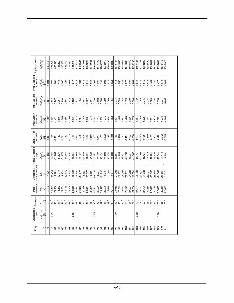
A-18

E

ntry

Dis

pla

cem

ent

L

eve

lP

ea

k D

efle

ctio

nD

efle

ctio

n a

t S

tart

of E

xcur

sio

nP

last

ic D

efle

ctio

n R

ang

eL

oa

d a

t Pe

ak

De

flect

ion

Ma

x. L

oa

d in

E

xcur

sio

nIn

itia

l Lo

ad

ing

S

tiffn

ess

Initi

al U

nlo

ad

ing

S

tiffn

ess

Hys

tere

sis

Are

a

(in.

) (+

/-)

i+i-

δ/δ

yδ

0/δ

yΔδ

pm/δ

yQ

/Qy

Qm

ax/Q

K0/

(Qy/δ

y)K

/(Q

y/δ

y)A

/(Q

y*δ

y)

[1]

[2]

[4]

[5]

[6]

[7]

[8]

[9]

[10

][1

1]

78

39

--1

9.6

93

12.6

72-2

7.5

61

-1.4

07

-1.4

07

0.1

57

0.9

93

80

8.1

66

79

2.2

54

0+

18

.29

1-1

4.86

82

9.4

80

1.3

31

1.3

61

0.1

13

1.0

00

83

1.8

05

80

40

--2

2.1

66

14.5

95-3

1.6

80

-1.4

21

-1.4

21

0.1

47

1.0

01

86

0.3

73

81

41

+1

8.2

10

-17.

077

31

.57

01

.33

91

.34

00

.09

71

.44

98

84

.23

2

82

41

--2

2.2

52

14.4

85-3

1.6

76

-1.3

81

-1.3

84

0.1

36

0.9

87

91

0.9

95

83

42

+1

8.1

85

-17.

175

31

.64

01

.31

21

.31

60

.10

11

.42

09

33

.71

2

84

42

--2

2.2

88

14.4

49-3

1.6

92

-1.3

53

-1.3

66

0.1

29

0.8

48

95

9.5

23

85

2.5

04

3+

20

.30

8-1

7.23

63

3.7

22

1.3

66

1.3

67

0.1

02

1.5

47

98

4.2

45

86

43

--2

4.7

57

16.4

70-3

5.9

63

-1.4

01

-1.4

13

0.1

17

0.8

79

10

14

.31

1

87

44

+2

0.3

04

-19.

477

35

.94

21

.30

41

.34

70

.09

41

.10

81

03

9.5

31

88

44

--2

4.7

86

16.4

62-3

5.9

83

-1.3

74

-1.3

88

0.1

07

0.9

12

10

67

.95

7

89

45

+2

0.3

24

-19.

522

35

.99

91

.28

21

.32

60

.09

70

.94

11

09

2.2

29

90

45

--2

4.8

10

16.4

66-3

6.0

28

-1.3

66

-1.3

74

0.1

01

0.8

89

11

19

.62

8

91

2.7

54

6+

22

.52

1-1

9.55

83

8.1

71

1.3

36

1.3

72

0.0

98

0.9

06

11

46

.08

9

92

46

--2

7.2

39

18.5

97-4

0.4

37

-1.4

14

-1.4

15

0.1

02

0.9

31

11

77

.79

6

93

47

+2

2.5

25

-21.

820

40

.40

41

.35

61

.35

90

.09

01

.23

21

20

4.7

75

94

47

--2

7.2

96

18.5

80-4

0.5

02

-1.3

72

-1.3

75

0.0

89

0.9

00

12

34

.91

9

95

48

+2

2.5

16

-21.

909

40

.51

01

.31

61

.34

50

.09

91

.01

01

26

0.8

62

96

48

--2

7.3

04

18.6

01-4

0.6

00

-1.3

59

-1.3

59

0.0

94

0.9

50

12

90

.08

2

97

3.0

04

9+

24

.52

9-2

1.99

14

2.6

61

1.3

52

1.4

01

0.0

73

1.0

72

13

18

.12

1

98

49

--2

9.7

12

20.6

67-4

4.8

90

-1.4

55

-1.4

55

0.0

99

0.9

52

13

51

.58

8

99

50

+2

4.5

13

-24.

207

44

.89

81

.36

21

.38

30

.06

81

.03

01

38

0.0

44

10

05

0-

-29

.77

320

.667

-45

.19

6-1

.40

1-1

.40

40

.09

90

.87

71

41

1.8

85

10

15

1+

-24

.52

1-2

4.52

14

5.2

61

0.0

00

1.3

60

0.0

39

0.0

39

14

39

.37

6

10

25

1-

-29

.80

620

.720

-45

.36

7-1

.35

8-1

.37

60

.09

60

.80

31

47

0.2

90

10

33

.00

52

+-2

4.6

31

-24.

631

45

.31

40

.00

01

.34

70

.04

20

.04

21

49

7.1

01

10

45

2-

-29

.84

720

.662

-45

.36

3-1

.34

3-1

.34

60

.08

50

.92

51

52

7.1

09

10

55

3+

-24

.70

0-2

4.70

04

5.4

28

0.0

01

1.3

23

0.0

45

0.0

45

15

53

.26

7

10

65

3-

-30

.38

920

.707

-46

.07

6-0

.84

0-1

.08

10

.07

40

.61

81

58

2.4

50

10

75

4+

27

.68

3-2

5.35

24

7.7

26

0.5

70

0.5

71

0.0

50

0.4

00

15

99

.50

7

10

85

4-

-31

.06

522

.349

-46

.92

8-0

.57

3-0

.57

80

.03

60

.18

11

61

4.0

56

10

93

.00

55

+2

7.6

38

-24.

566

46

.54

00

.54

90

.54

90

.03

80

.42

71

62

6.6

91

11

05

5-

-29

.65

521

.958

-18

.47

9-0

.01

2-0

.23

30

.03

70

.01

91

63

5.4

13

11

15

6+

28

.68

93.

525

#N

/A-0

.00

5-0

.00

6-0

.00

20

.00

01

63

5.3

25

[3]

Exc

ursi

on

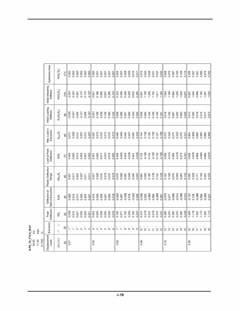
A-19

S-P

6_T

4_

FT

2.4

_W

-01

50

.00

ksi

11

.40

kip

s

0.1

162

in.

Dis

pla

cem

ent

Leve

lP

eak

D

efle

ctio

nD

efle

ctio

n a

t S

tart

of E

xcur

sion

Pla

stic

De

flect

ion

Ran

ge

Lo

ad

at P

eak

Def

lect

ion

Ma

x. L

oad

in

Exc

ursi

on

Initi

al L

oa

din

g S

tiffn

ess

Initi

al U

nlo

adi

ng

Stif

fne

ssH

yste

resi

s A

rea

(in.

) (+

/-)

i+i-

δ/δ

yδ 0

/δy

Δδ

pm/δ

yQ

/Qy

Qm

ax/Q

K0/

(Qy/δ

y)K

/(Q

y/δ

y)A

/(Q

y*δ

y)

[2]

[4]

[5]

[6]

[7]

[8]

[9]

[10]

[11]

0.0

11

+-0

.02

80.

000

0.0

07

0.0

00

0.0

13-0

.00

5-0

.00

10.

00

0

1-

0.0

140.

014

-0.0

11

0.0

00

-0.0

08

-0.3

01

-0.3

01

0.0

00

2+

0.0

210.

011

0.0

04

0.0

12

0.0

120

.42

60

.39

10.

00

0

2-

0.0

250.

025

-0.0

07

0.0

00

-0.0

07

-0.1

21

-0.1

21

0.0

00

3+

0.0

250.

007

0.0

11

0.0

07

0.0

120

.29

90

.17

20.

00

0

3-

0.0

210.

021

-0.0

11

0.0

00

-0.0

07

-0.1

67

-0.1

67

0.0

00

0.0

24

+0

.054

0.01

40.

00

70

.00

10

.020

-0.0

21

0.0

01

0.0

00

4-

0.0

250.

025

-0.0

28

0.0

00

-0.0

15

0.1

86

0.1

86

0.0

01

5+

0.0

390.

004

0.0

18

0.0

17

0.0

190

.33

90

.26

50.

00

1

5-

0.0

250.

021

-0.0

18

-0.0

01-0

.01

30

.10

80

.06

70.

00

1

6+

0.0

320.

000

0.0

18

0.0

18

0.0

190

.38

00

.39

50.

00

1

6-

0.0

180.

018

-0.0

18

0.0

00

-0.0

12

0.1

04

0.1

04

0.0

01

0.0

37

+0

.100

-0.0

040.

07

80

.04

60

.046

0.0

08

0.3

23

0.0

04

7-

0.0

710.

057

-0.0

96

-0.0

02-0

.05

50

.38

90

.39

90.

00

7

8+

0.1

00-0

.028

0.0

50

0.0

43

0.0

460

.35

10

.42

60.

00

8

8-

-0.0

54

0.01

8-0

.04

6-0

.038

-0.0

47

0.5

90

0.4

09

0.0

09

9+

0.1

00-0

.032

0.0

46

0.0

41

0.0

450

.34

30

.63

20.

01

0

9-

-0.0

57

0.02

5-0

.05

7-0

.035

-0.0

44

0.5

55

0.3

65

0.0

11

0.0

61

0+

0.2

10-0

.036

0.0

64

0.1

32

0.1

340

.05

90

.95

10.

01

5

10

--0

.21

80.

025

-0.0

93

-0.1

58-0

.15

80

.58

31

.15

90.

02

2

11

+0

.210

-0.0

640.

13

60

.13

40

.136

0.1

64

1.2

65

0.0

26

11

--0

.21

80.

064

-0.1

39

-0.1

58-0

.15

80

.16

91

.10

20.

03

1

12

+0

.210

-0.0

680.

13

20

.13

00

.137

0.1

64

1.8

11

0.0

37

12

--0

.22

10.

061

-0.1

28

-0.1

58-0

.15

80

.18

11

.16

40.

04

2

0.1

01

3+

0.3

89-0

.075

0.1

53

0.2

56

0.2

720

.01

91

.04

40.

05

8

13

--0

.42

10.

071

-0.1

68

-0.3

14-0

.32

40

.18

21

.18

90.

07

6

14

+0

.392

-0.0

860.

07

80

.26

00

.275

0.0

67

0.9

64

0.0

87

14

--0

.42

1-0

.014

-0.0

93

-0.3

18-0

.32

20

.45

21

.25

50.

10

0

15

+0

.392

-0.0

960.

08

90

.27

30

.275

0.0

63

1.0

64

0.1

09

15

--0

.43

5-0

.014

-0.1

32

-0.3

21-0

.32

10

.45

50

.83

70.

11

5

0.2

51

6+

1.2

48-0

.157

0.2

85

0.8

38

0.8

640

.01

30

.90

70.

25

6

16

--1

.11

60.

125

-0.2

28

-0.8

78-0

.88

60

.39

51

.04

40.

39

7

17

+1

.252

-0.0

960.

17

10

.88

80

.888

0.0

19

0.9

69

0.4

91

17

--1

.11

30.

064

-0.1

64

-0.8

84-0

.88

70

.31

41

.18

20.

58

5

18

+1

.245

-0.0

930.

32

50

.88

60

.889

0.0

17

1.0

81

0.6

72

18

--1

.11

30.

221

-0.3

25

-0.8

79-0

.88

50

.07

31

.03

00.

76

2

Exc

ursi

on

[3]

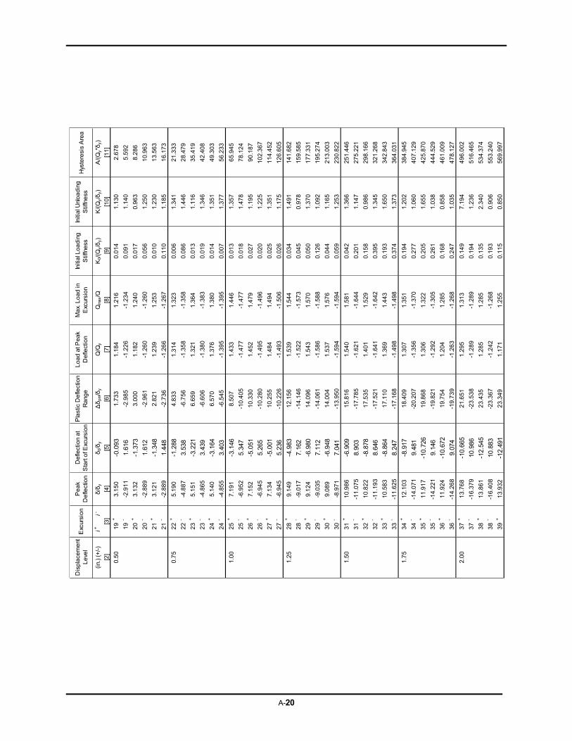
A-20

D

isp

lace

me

nt

Le

vel

Pe

ak

De

flect

ion

De

flect

ion

at

Sta

rt o

f Exc

ursi

on

Pla

stic

De

flect

ion

Ra

nge

Lo

ad

at P

ea

k D

efle

ctio

nM

ax.

Lo

ad

in

Exc

ursi

on

Initi

al L

oa

din

g

Stif

fne

ssIn

itia

l Unl

oa

din

g

Stif

fne

ssH

yste

resi

s A

rea

(in.

) (+

/-)

i+i-

δ/δ

yδ

0/δ

yΔδ

pm/δ

yQ

/Qy

Qm

ax/Q

K0/

(Qy/δ

y)K

/(Q

y/δ

y)A

/(Q

y*δ

y)

[2]

[4]

[5]

[6]

[7]

[8]

[9]

[10

][1

1]

0.5

01

9+

3.1

50

-0.0

931

.73

31

.18

41

.21

60

.01

41

.13

02

.67

8

19

--2

.91

11.

616

-2.9

85

-1.2

26

-1.2

34

0.0

91

1.1

40

5.5

92

20

+3

.13

2-1

.373

3.0

00

1.1

82

1.2

40

0.0

17

0.9

63

8.2

86

20

--2

.88

91.

612

-2.9

61

-1.2

60

-1.2

60

0.0

56

1.2

50

10

.96

3

21

+3

.12

1-1

.348

2.8

21

1.2

39

1.2

53

0.0

10

1.2

30

13

.56

3

21

--2

.88

91.

448

-2.7

36

-1.2

66

-1.2

67

0.1

10

1.1

85

16

.17

3

0.7

52

2+

5.1

90

-1.2

884

.83

31

.31

41

.32

30

.00

61

.34

12

1.3

33

22

--4

.88

73.

538

-6.7

56

-1.3

58

-1.3

58

0.0

86

1.4

46

28

.47

9

23

+5

.15

1-3

.221

6.6

59

1.3

21

1.3

64

0.0

13

1.1

16

35

.41

9

23

--4

.86

53.

439

-6.6

06

-1.3

80

-1.3

83

0.0

19

1.3

46

42

.40

8

24

+5

.14

0-3

.164

6.5

70

1.3

76

1.3

80

0.0

14

1.3

51

49

.30

3

24

--4

.85

53.

403

-6.5

45

-1.3

95

-1.3

95

0.0

07

1.3

77

56

.23

3

1.0

02

5+

7.1

91

-3.1

468

.50

71

.43

31

.44

60

.01

31

.35

76

5.9

45

25

--6

.95

25.

347

-10

.40

5-1

.47

7-1

.47

70

.01

81

.47

87

8.1

24

26

+7

.15

2-5

.051

10

.33

01

.45

21

.47

90

.02

71

.19

59

0.1

87

26

--6

.94

55.

265

-10

.28

0-1

.49

5-1

.49

60

.02

01

.22

51

02

.36

7

27

+7

.13

4-5

.001

10

.25

51

.48

41

.49

40

.02

51

.35

11

14

.45

2

27

--6

.94

55.

236

-10

.22

6-1

.49

3-1

.50

60

.02

61

.17

51

26

.60

5

1.2

52

8+

9.1

49

-4.9

831

2.1

56

1.5

39

1.5

44

0.0

34

1.4

91

14

1.6

82

28

--9

.01

77.

162

-14

.14

6-1

.52

2-1

.57

30

.04

50

.97

81

59

.58

5

29

+9

.12

4-6

.980

14

.09

61

.54

31

.57

00

.05

01

.37

01

77

.33

1

29

--9

.03

57.

112

-14

.06

1-1

.58

6-1

.58

80

.12

61

.09

21

95

.27

4

30

+9

.08

9-6

.948

14

.00

41

.53

71

.57

60

.04

41

.16

52

13

.00

3

30

--8

.97

17.

041

-13

.95

0-1

.59

4-1

.59

40

.05

91

.25

32

30

.82

2

1.5

03

1+

10

.98

6-6

.909

15

.81

61

.54

01

.58

10

.04

21

.36

62

51

.44

6

31

--1

1.0

75

8.90

3-1

7.7

85

-1.6

21

-1.6

44

0.2

01

1.1

47

27

5.2

21

32

+1

0.8

22

-8.8

781

7.5

35

1.4

01

1.5

29

0.1

58

0.9

86

29

8.1

66

32

--1

1.1

93

8.64

6-1

7.5

21

-1.6

41

-1.6

42

0.3

95

1.3

45

32

1.2

68

33

+1

0.5

83

-8.8

641

7.1

10

1.3

69

1.4

43

0.1

93

1.6

50

34

2.8

43

33

--1

1.6

25

8.24

7-1

7.1

68

-1.4

98

-1.4

98

0.3

74

1.3

73

36

4.0

31

1.7

53

4+

12

.10

3-8

.917

18

.40

91

.30

71

.35

10

.19

41

.20

23

84

.94

5

34

--1

4.0

71

9.48

1-2

0.2

07

-1.3

56

-1.3

70

0.2

77

1.0

60

40

7.1

29

35

+1

1.9

17

-10.

726

19

.86

81

.30

61

.32

20

.20

51

.65

54

25

.87

0

35

--1

4.2

21

9.14

6-1

9.8

21

-1.2

92

-1.3

05

0.2

61

1.0

38

44

4.5

29

36

+1

1.9

24

-10.

672

19

.75

41

.20

41

.28

50

.16

80

.85

84

61

.00

9

36

--1

4.2

68

9.07

4-1

9.7

39

-1.2

63

-1.2

68

0.2

47

1.0

35

47

8.1

27

2.0

03

7+

13

.76

8-1

0.66

52

1.6

51

1.2

95

1.3

13

0.1

49

7.1

94

49

6.0

02

37

--1

6.3

79

10.9

86-2

3.5

38

-1.2

89

-1.2

89

0.1

94

1.2

36

51

6.4

65

38

+1

3.8

61

-12.

545

23

.43

51

.28

51

.28

50

.13

52

.34

05

34

.37

4

38

--1

6.4

08

10.8

83-2

3.3

67

-1.2

42

-1.2

68

0.1

93

0.9

06

55

3.2

40

39

+1

3.9

32

-12.

491

23

.34

91

.17

11

.25

50

.11

50

.85

05

69

.99

7

Exc

ursi

on

[3]

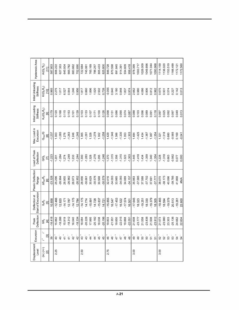
A-21

D

isp

lace

me

nt

Le

vel

Pe

ak

De

flect

ion

De

flect

ion

at

Sta

rt o

f Exc

ursi

on

Pla

stic

De

flect

ion

Ra

nge

Lo

ad

at P

ea

k D

efle

ctio

nM

ax.

Lo

ad

in

Exc

ursi

on

Initi

al L

oa

din

g

Stif

fne

ssIn

itia

l Unl

oa

din

g

Stif

fne

ssH

yste

resi

s A

rea

(in.

) (+

/-)

i+i-

δ/δ

yδ

0/δ

yΔδ

pm/δ

yQ

/Qy

Qm

ax/Q

K0/

(Qy/δ

y)K

/(Q

y/δ

y)

A/(

Qy*δ

y)

[2]

[4]

[5]

[6]

[7]

[8]

[9]

[10

][1

1]

39

--1

6.4

18

10.8

58-2

3.3

28

-1.2

23

-1.2

37

0.1

79

0.9

65

58

7.8

03

2.2

54

0+

15

.86

2-1

2.46

62

5.2

96

1.2

01

1.3

03

0.1

20

2.2

75

60

6.2

22

40

--1

8.2

88

12.8

20-2

6.9

94

-1.2

84

-1.2

85

0.1

68

1.0

17

62

7.3

53

41

+1

5.9

19

-14.

171

26

.95

51

.27

41

.27

60

.11

56

.52

76

45

.93

4

41

--1

8.3

12

12.7

87-2

6.9

62

-1.2

49

-1.2

63

0.1

53

0.8

44

66

5.7

82

42

+1

6.0

40

-14.

175

26

.97

31

.23

31

.24

60

.10

11

.24

66

83

.66

2

42

--1

8.3

34

12.7

84-2

6.9

52

-1.2

44

-1.2

46

0.1

39

0.9

56

70

2.6

90

2.5

04

3+

18

.08

4-1

4.17

52

8.9

56

1.3

00

1.3

65

0.1

03

1.8

17

72

2.6

84

43

--2

0.2

28

14.7

74-3

0.6

61

-1.2

83

-1.2

91

0.1

33

0.8

60

74

5.0

61

44

+1

7.9

95

-15.

891

30

.62

91

.32

81

.32

80

.10

71

.89

67

65

.16

9

44

--2

0.1

82

14.7

28-3

0.5

76

-1.2

78

-1.2

78

0.1

71

1.0

20

78

6.2

57

45

+1

8.0

38

-15.

837

30

.56

81

.29

51

.30

20

.10

02

.50

28

05

.43

3

45

--2

0.1

96

14.7

21-3

0.5

79

-1.2

48

-1.2

58

0.1

26

0.7

39

82

5.8

00

2.7

54

6+

19

.80

3-1

5.85

53

2.4

16

1.3

70

1.4

29

0.0

98

-0.0

55

84

6.7

28

46

--2

1.9

51

16.5

47-3

4.0

03

-1.3

15

-1.3

46

0.1

31

0.8

40

87

0.5

98

47

+1

9.8

50

-17.

453

33

.98

51

.35

61

.38

60

.08

63

.18

08

91

.84

5

47

--2

2.0

15

16.5

22-3

4.0

93

-1.3

15

-1.3

30

0.0

90

0.8

48

91

4.3

91

48

+1

9.8

68

-17.

574

34

.08

91

.32

31

.35

30

.07

41

.83

79

34

.60

9

48

--2

2.0

51

16.5

01-3

4.1

57

-1.3

03

-1.3

03

0.0

87

0.9

74

95

6.4

18

3.0

04

9+

21

.60

8-1

7.64

53

5.9

83

1.4

45

1.4

84

0.0

88

2.6

62

97

8.3

99

49

--2

3.7

77

18.3

23-3

7.5

85

-1.4

18

-1.4

25

0.1

03

0.9

80

10

03

.71

7

50

+2

1.5

58

-19.

251

37

.58

81

.43

41

.43

40

.09

64

.08

61

02

6.0

09

50

--2

3.8

38

18.3

30-3

7.7

02

-1.3

59

-1.3

87

0.0

89

0.8

06

10

49

.89

6

51

+2

1.5

08

-19.

379

37

.69

11

.34

01

.38

70

.09

10

.81

21

07

1.0

44

51

--2

3.9

12

18.3

05-3

7.7

77

-1.3

54

-1.3

54

0.1

18

0.9

62

10

93

.96

8

3.0

05

2+

21

.57

3-1

9.46

53

8.0

70

1.2

28

1.3

21

0.0

97

0.6

75

11

14

.15

9

52

--2

3.9

80

18.5

94-3

8.1

73

-1.3

18

-1.3

18

0.0

25

0.9

31

11

36

.02

0

53

+2

3.3

03

-19.

579

40

.09

60

.66

30

.68

00

.09

20

.57

41

15

3.5

19

53

--2

5.1

36

20.5

13-3

9.7

85

-0.5

62

-0.5

65

0.0

97

0.2

27

11

66

.49

9

54

+2

4.6

62

-19.

261

41

.86

80

.07

70

.16

90

.04

90

.14

21

17

2.1

21

54

-2

2.6

04

22.6

00#

N/A

0.0

00

-0.0

41

0.0

13

0.0

13

11

72

.56

0

[3]

Exc

ursi

on

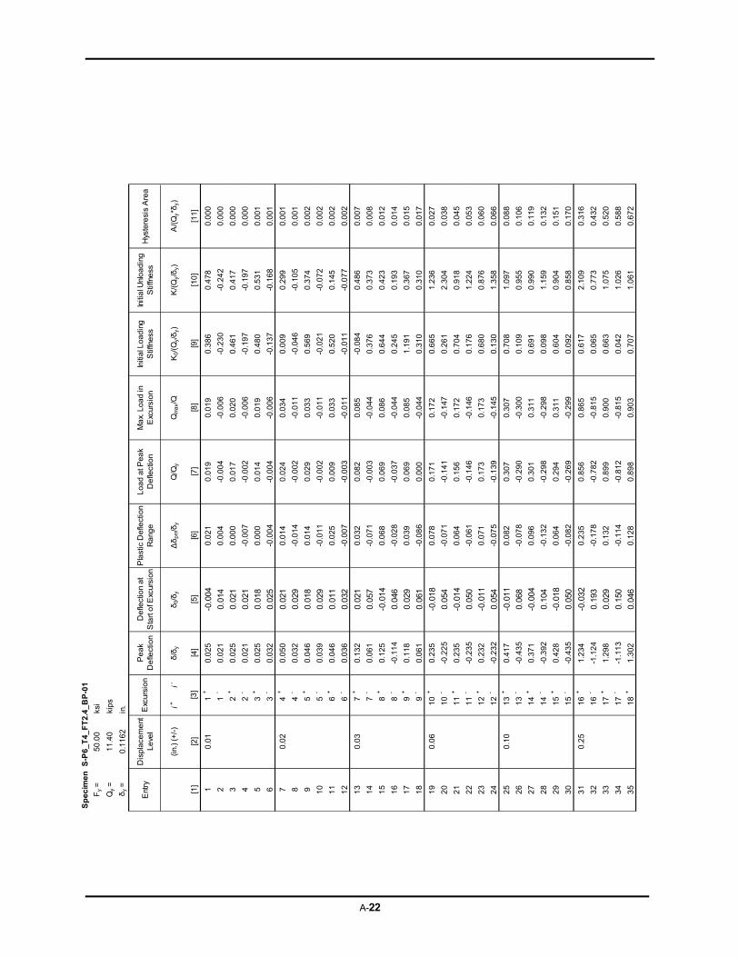
A-22

Sp

ec

ime

nS

-P6

_T

4_

FT

2.4

_B

P-0

1

Fy

=5

0.0

0ks

i

Qy

=1

1.4

0ki

ps

δy

=0

.11

62

in.

Ent

ryD

isp

lace

me

nt

Le

vel

Pe

ak

De

flect

ion

De

flect

ion

at

Sta

rt o

f Exc

ursi

on

Pla

stic

De

flect

ion

Ra

nge

Lo

ad

at P

ea

k D

efle

ctio

nM

ax.

Lo

ad

in

Exc

ursi

on

Initi

al L

oa

din

g

Stif

fne

ssIn

itia

l Unl

oa

din

g

Stif

fne

ssH

yste

resi

s A

rea

(in.

) (+

/-)

i+i-

δ/δ

yδ

0/δ

yΔδ

pm/δ

yQ

/Qy

Qm

ax/Q

K0/

(Qy/δ

y)K

/(Q

y/δ

y)A

/(Q

y*δ

y)

[1]

[2]

[4]

[5]

[6]

[7]

[8]

[9]

[10

][1

1]

10

.01

1+

0.0

25

-0.0

040

.02

10

.01

90

.01

90

.38

60

.47

80

.00

0

21

-0

.02

10.

014

0.0

04

-0.0

04

-0.0

06

-0.2

30

-0.2

42

0.0

00

32

+0

.02

50.

021

0.0

00

0.0

17

0.0

20

0.4

61

0.4

17

0.0

00

42

-0

.02

10.

021

-0.0

07

-0.0

02

-0.0

06

-0.1

97

-0.1

97

0.0

00

53

+0

.02

50.

018

0.0

00

0.0

14

0.0

19

0.4

80

0.5

31

0.0

01

63

-0

.03

20.

025

-0.0

04

-0.0

04

-0.0

06

-0.1

37

-0.1

68

0.0

01

70

.02

4+

0.0

50

0.02

10

.01

40

.02

40

.03

40

.00

90

.29

90

.00

1

84

-0

.03

20.

029

-0.0

14

-0.0

02

-0.0

11

-0.0

46

-0.1

05

0.0

01

95

+0

.04

60.

018

0.0

14

0.0

29

0.0

33

0.5

69

0.3

74

0.0

02

10

5-

0.0

39

0.02

9-0

.01

1-0

.00

2-0

.01

1-0

.02

1-0

.07

20

.00

2

11

6+

0.0

46

0.01

10

.02

50

.00

90

.03

30

.52

00

.14

50

.00

2

12

6-

0.0

36

0.03

2-0

.00

7-0

.00

3-0

.01

1-0

.01

1-0

.07

70

.00

2

13

0.0

37

+0

.13

20.

021

0.0

32

0.0

82

0.0

85

-0.0

84

0.4

86

0.0

07

14

7-

0.0

61

0.05

7-0

.07

1-0

.00

3-0

.04

40

.37

60

.37

30

.00

8

15

8+

0.1

25

-0.0

140

.06

80

.06

90

.08

60

.64

40

.42

30

.01

2

16

8-

-0.1

14

0.04

6-0

.02

8-0

.03

7-0

.04

40

.24

50

.19

30

.01

4

17

9+

0.1

18

0.02

90

.03

90

.06

90

.08

51

.19

10

.36

70

.01

5

18

9-

0.0

61

0.06

1-0

.08

60

.00

0-0

.04

40

.31

00

.31

00

.01

7

19

0.0

61

0+

0.2

35

-0.0

180

.07

80

.17

10

.17

20

.66

51

.23

60

.02

7

20

10

--0

.22

50.

054

-0.0

71

-0.1

41

-0.1

47

0.2

61

2.3

04

0.0

38

21

11

+0

.23

5-0

.014

0.0

64

0.1

56

0.1

72

0.7

04

0.9

18

0.0

45

22

11

--0

.23

50.

050

-0.0

61

-0.1

46

-0.1

46

0.1

76

1.2

24

0.0

53

23

12

+0

.23

2-0

.011

0.0

71

0.1

73

0.1

73

0.6

80

0.8

76

0.0

60

24

12

--0

.23

20.

054

-0.0

75

-0.1

39

-0.1

45

0.1

30

1.3

58

0.0

66

25

0.1

01

3+

0.4

17

-0.0

110

.08

20

.30

70

.30

70

.70

81

.09

70

.08

8

26

13

--0

.43

50.

068

-0.0

78

-0.2

90

-0.3

00

0.1

09

0.9

55

0.1

06

27

14

+0

.37

1-0

.004

0.0

96

0.3

01

0.3

11

0.6

91

0.9

90

0.1

19

28

14

--0

.39

20.

104

-0.1

32

-0.2

98

-0.2

98

0.0

98

1.1

59

0.1

32

29

15

+0

.42

8-0

.018

0.0

64

0.2

94

0.3

11

0.6

04

0.9

04

0.1

51

30

15

--0

.43

50.

050

-0.0

82

-0.2

69

-0.2

99

0.0

92

0.8

58

0.1

70

31

0.2

51

6+

1.2

34

-0.0

320

.23

50

.85

60

.86

50

.61

72

.10

90

.31

6

32

16

--1

.12

40.

193

-0.1

78

-0.7

82

-0.8

15

0.0

65

0.7

73

0.4

32

33

17

+1

.29

80.

029

0.1

32

0.8

99

0.9

00

0.6

63

1.0

75

0.5

20

34

17

--1

.11

30.

150

-0.1

14

-0.8

12

-0.8

15

0.0

42

1.0

26

0.5

88

35

18

+1

.30

20.

046

0.1

28

0.8

98

0.9

03

0.7

07

1.0

61

0.6

72

Exc

ursi

on

[3]

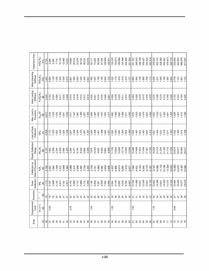
A-23

Ent

ryD

isp

lace

me

nt

Le

vel

Pe

ak

Def

lect

ion

De

flect

ion

at

Sta

rt o

f Exc

ursi

on

Pla

stic

De

flect

ion

Ra

nge

Lo

ad

at P

ea

k D

efle

ctio

nM

ax.

Lo

ad

in

Exc

ursi

on

Initi

al L

oa

din

g

Stif

fne

ssIn

itia

l Unl

oa

din

g

Stif

fne

ssH

yste

resi

s A

rea

(in.

) (+

/-)

i+i-

δ/δ

yδ

0/δ

yΔδ

pm/δ

yQ

/Qy

Qm

ax/Q

K0/

(Qy/δ

y)K

/(Q

y/δ

y)A

/(Q

y*δ

y)

[1]

[2]

[4]

[5]

[6]

[7]

[8]

[9]

[10

][1

1]

36

18

--1

.11

60.

150

-0.1

07

-0.8

08

-0.8

13

0.0

34

1.0

03

0.7

39

37

0.5

01

9+

3.1

50

0.05

71

.55

21

.17

21

.21

80

.74

20

.98

32

.58

9

38

19

--2

.88

91.

584

-2.8

29

-1.2

25

-1.2

25

0.0

23

1.1

39

5.2

66

39

20

+3

.13

5-1

.248

2.7

64

1.2

03

1.2

35

0.0

95

1.0

36

7.7

19

40

20

--2

.87

11.

512

-2.5

25

-1.2

45

-1.2

45

0.0

17

1.2

20

10

.14

3

41

21

+3

.13

2-0

.999

2.4

86

1.2

29

1.2

47

0.5

32

1.0

34

12

.48

9

42

21

--2

.87

11.

484

-2.4

83

-1.2

36

-1.2

52

0.0

48

0.9

15

14

.83

7

43

0.7

52

2+

5.1

76

-0.9

884

.39

41

.25

71

.31

70

.51

30

.80

11

9.6

86

44

22

--4

.88

03.

414

-6.2

71

-1.3

46

-1.3

47

0.0

16

1.3

60

26

.53

4

45

23

+5

.11

5-2

.846

6.1

39

1.3

09

1.3

62

0.5

18

0.9

50

33

.07

6

46

23

--4

.86

93.

285

-6.0

42

-1.3

74

-1.3

80

0.0

14

1.2

20

39

.72

5

47

24

+5

.11

5-2

.754

5.9

96

1.3

87

1.3

87

0.5

17

1.3

93

46

.22

3

48

24

--4

.86

53.

235

-5.9

46

-1.3

57

-1.3

94

0.0

15

0.9

21

52

.81

8

49

1.0

02

5+

7.1

30

-2.7

007

.87

61

.45

01

.45

80

.53

21

.28

26

2.1

17

50

25

--6

.95

25.

161

-10

.02

7-1

.45

8-1

.48

70

.02

11

.05

77

3.9

50

51

26

+7

.08

7-4

.862

9.9

30

1.4

81

1.4

93

0.0

14

1.1

96

85

.54

6

52

26

--6

.95

95.

062

-9.9

02

-1.4

96

-1.5

07

0.0

35

1.1

82

97

.33

8

53

27

+7

.05

9-4

.833

9.8

55

1.4

59

1.5

05

0.0

48

0.9

24

10

8.9

00

54

27

--6

.98

45.

008

-9.8

59

-1.5

01

-1.5

17

0.0

51

1.1

22

12

0.6

71

55

1.2

52

8+

9.0

64

-4.8

371

1.7

28

1.5

26

1.5

60

0.0

68

1.0

22

13

5.2

25

56

28

--9

.14

96.

888

-13

.80

4-1

.54

0-1

.58

00

.23

91

.17

21

52

.81

4

57

29

+8

.92

8-6

.913

13

.60

81

.58

01

.58

00

.22

01

.47

81

69

.88

6

58

29

--9

.30

26.

695

-13

.71

5-1

.50

4-1

.56

60

.41

11

.01

61

87

.49

8

59

30

+8

.79

6-7

.016

13

.59

31

.55

41

.57

70

.27

21

.21

02

04

.46

0

60

30

--9

.46

76.

577

-13

.65

4-1

.49

2-1

.54

20

.43

41

.12

12

21

.92

4

61

1.5

03

1+

10

.76

9-7

.062

15

.49

81

.52

81

.57

90

.36

30

.89

42

41

.78

7

62

31

--1

1.8

85

8.43

2-1

7.6

06

-1.4

97

-1.5

23

0.3

95

1.5

54

26

5.0

03

63

32

+1

0.6

51

-9.1

631

7.4

03

1.5

24

1.5

62

0.2

76

1.1

48

28

6.7

98

64

32

--1

2.0

45

8.24

0-1

7.4

46

-1.4

61

-1.4

74

0.4

15

1.5

60

30

9.3

27

65

33

+1

0.6

51

-9.1

781

7.3

67

1.5

52

1.5

53

0.2

79

1.7

69

33

0.4

22

66

33

--1

2.1

02

8.18

3-1

7.3

53

-1.4

15

-1.4

44

0.3

76

1.1

13

35

2.4

18

67

1.7

53

4+

12

.65

2-9

.167

19

.25

41

.55

11

.55

30

.27

52

.00

53

76

.00

3

68

34

--1

4.2

89

10.0

80-2

1.2

12

-1.4

04

-1.4

33

0.3

36

1.2

31

40

3.1

47

69

35

+1

2.8

41

-11.

132

21

.33

41

.57

01

.57

70

.21

91

.55

54

28

.38

5

70

35

--1

4.4

00

10.1

98-2

1.3

02

-1.4

16

-1.4

20

0.3

12

1.1

85

45

5.0

61

71

36

+1

3.3

15

-11.

093

21

.71

51

.57

11

.59

10

.19

01

.38

74

79

.97

3

72

36

--1

4.4

39

10.6

22-2

1.6

26

-1.3

62

-1.4

05

0.3

26

0.9

04

50

6.1

78

73

2.0

03

7+

15

.48

4-1

0.99

32

3.6

74

1.4

32

1.5

26

0.1

53

0.7

76

53

2.6

54

74

37

--1

6.6

32

12.6

70-2

5.5

71

-1.3

82

-1.4

07

0.3

24

1.1

47

56

2.6

52

75

38

+1

5.2

77

-12.

901

25

.48

91

.51

31

.51

30

.18

31

.80

15

88

.97

8

76

38

--1

6.6

18

12.5

84-2

5.4

11

-1.3

59

-1.3

65

0.3

05

1.1

32

61

7.0

07

Exc

ursi

on

[3]

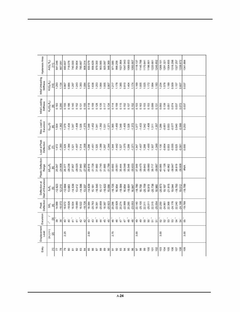
A-24

Ent

ryD

ispl

ace

me

nt

Lev

el

Pea

k D

efle

ctio

nD

efle

ctio

n at

S

tart

of E

xcur

sio

nP

last

ic D

efle

ctio

n R

ang

eLo

ad a

t Pe

ak

De

flect

ion

Max

. Loa

d in

E

xcur

sio

nIn

itial

Loa

ding

S

tiffn

ess

Initi

al U

nlo

adin

g S

tiffn

ess

Hys

tere

sis

Are

a

(in.

) (+

/-)

i+i-

δ/δ

yδ 0

/δy

Δδ

pm/δ

yQ

/Qy

Qm

ax/Q

K0/

(Qy/δ

y)K

/(Q

y/δ y

)A

/(Q

y*δ

y)

[1]

[2]

[4]

[5]

[6]

[7]

[8]

[9]

[10]

[11]

77

39+

14.

988

-12.

823

25.0

47

1.4

721

.50

40

.18

31

.29

364

1.0

46

78

39-

-16

.57

212

.210

-24.

908

-1.3

60-1

.362

0.2

90

1.1

34

667.

091

79

2.2

540

+1

6.6

72-1

2.68

426

.37

71.

329

1.3

79

0.1

55

0.8

67

690.

607

80

40-

-18

.62

613

.683

-28.

236

-1.3

84-1

.434

0.1

86

0.8

84

718.

076

81

41+

16.

504

-14.

539

27.9

57

1.3

211

.34

70

.14

01

.29

774

0.5

00

82

41-

-18

.68

013

.412

-28.

025

-1.4

07-1

.408

0.1

52

1.2

43

764.

804

83

42+

16.

522

-14.

596

27.9

40

1.3

141

.32

60

.13

11

.39

378

5.6

67

84

42-

-18

.72

613

.337

-27.

982

-1.3

58-1

.370

0.1

55

1.0

84

808.

314

85

2.5

043

+1

8.3

84-1

4.63

929

.81

61.

296

1.3

48

0.1

18

0.8

70

830.

579

86

43-

-20

.76

315

.181

-31.

728

-1.4

51-1

.452

0.1

59

1.6

36

856.

629

87

44+

18.

391

-16.

540

31.6

60

1.3

201

.34

10

.12

81

.25

387

9.3

00

88

44-

-20

.85

915

.117

-31.

745

-1.3

86-1

.392

0.1

35

1.0

64

903.

565

89

45+

18.

387

-16.

622

31.6

85

1.2

971

.33

10

.11

71

.00

592

5.0

97

90

45-

-20

.92

315

.056

-31.

799

-1.3

44-1

.371

0.1

34

0.9

07

948.

369

91

2.7

546

+2

0.2

96-1

6.72

533

.69

31.

344

1.3

65

0.1

14

1.2

17

971.

585

92

46-

-22

.92

816

.954

-35.

551

-1.4

42-1

.450

0.1

59

1.1

78

998.

258

93

47+

20.

274

-18.

584

35.4

44

1.3

271

.34

80

.11

51

.38

510

21.8

64

94

47-

-22

.99

916

.854

-35.

548

-1.3

75-1

.405

0.1

52

0.9

10

1047

.04

3

95

48+

20.

285

-18.

691

35.5

48

1.2

991

.32

80

.10

71

.40

410

69.6

53

96

48-

-23

.05

316

.847

-35.

633

-1.3

71-1

.372

0.1

52

1.1

74

1093

.90

7

97

3.0

049

+2

2.1

40-1

8.78

037

.54

91.

347

1.3

77

0.1

03

1.1

69

1118

.13

7

98

49-

-25

.10

018

.758

-39.

475

-1.4

07-1

.433

0.1

63

1.0

05

1145

.78

8

99

50+

22.

311

-20.

709

39.6

43

1.2

881

.34

20

.10

31

.02

511

70.6

41

100

50-

-25

.01

118

.919

-39.

660

-1.4

00-1

.408

0.1

53

1.1

72

1196

.90

1

101

51+

22.

315

-20.

738

39.7

17

1.3

071

.31

10

.09

91

.99

412

20.6

61

102

51-

-25

.05

418

.980

-39.

867

-1.3

49-1

.357

0.1

31

1.1

83

1245

.85

2

103

3.0

052

+2

2.2

50-2

0.87

340

.08

51.

130

1.2

86

0.0

93

1.2

34

1269

.10

1

104

52-

-24

.86

119

.197

-41.

126

-0.8

04-0

.851

0.1

39

1.5

78

1291

.32

1

105

53+

22.

368

-21.

915

40.9

62

0.5

530

.55

30

.05

11

.18

913

04.6

55

106

53-

-24

.17

619

.044

-38.

847

-0.5

55-0

.577

0.0

74

0.5

09

1316

.29

8

107

54+

22.

240

-19.

793

38.8

19

0.5

250

.54

00

.03

71

.15

713

27.2

57

108

54-

-24

.19

819

.012

-38.

808

-0.5

61-0

.566

0.0

72

0.6

07

1338

.67

2

109

3.0

055

+-1

9.7

89

-19.

789

#N/A

0.0

000

.25

30

.03

70

.03

713

41.8

84

Exc

ursi

on

[3]