IAPRS, Vol. XXXIII, Amsterdam, 2000

HYBRID MODELLING AND ANALYSIS OF UNCERTAIN DATA

Michael GLEMSER, Ulrike KLEINInstitute for Photogrammetry (ifp), Stuttgart University, Germany

Geschwister-Scholl-Strasse 24D, D-70174 StuttgartMichael.Glemser@ifp.uni-stuttgart.de

Ulrike.Klein@ifp.uni-stuttgart.de

Working Group IV/III.1

KEY WORDS: Data Uncertainty, Object-Oriented Modelling, Hybrid Analysis Methods, Uncertainty Propagation.

ABSTRACT

An essential requirement for a comprehensive use of hybrid data is the consideration and processing of its uncertainty.Erroneous interpretations of analyses can be avoided if uncertainty is integrated as a mandatory component, stored andconsidered in all operations. In this contribution, a probabilistic approach is presented for modelling geometric andthematic uncertainty. By means of a flooding forecast as an example application, the enhancements which are necessaryin data modelling and analysis functions are explained.

1 INTRODUCTION

Over the years, GIS have evolved to powerful tools which solve various tasks in a variety of different applications. Theongoing integration of new and improved analysis methods enables users to process even more complex applicationtasks with combinations of geometrical, topological and thematic aspects using hybrid data, i. e. raster data as well asvector data. A further step in development will be achieved by the opening of the architecture to interoperable systems(McKee and Kuhn, 1997, OGC, 1999, IOGIS, 1999). In such an open environment, the problems are distributed amongdifferent systems which act like single components. The final result is obtained in this teamwork-like approach by acombination where each component adds its part.

Data uncertainty plays a special role in such an environment. Although all data is uncertain to a particular degree, thenecessary integration in GIS has not taken place so far. The consequence is that uncertainty is actually not taken intoaccount during data processing. This kind of disregard can partly be justified only in the case of a closed system, wherethe user has full control over all steps from input to presentation. As the user is aware of the data quality, he is able toverify the result using his knowledge and experience. This might be seen as a reason why uncertainty has not been arelevant topic in GIS yet. But the control gets completely lost in an interoperable system. This starts already within thedata input step. Today, a great number of existing databases offer a variety of data sets like topographic information,cadastral data, statistical data or digital orthophotos and satellite images. Data collection is changing widely fromdigitising own data to retrieving and transferring it from existing data bases. For such data sets, the user requires anuncertainty description which has to be added by the producer of the data set as a kind of meta description. Thisinformation allows the data to be checked in order to avoid the risk of combinations of data without any practical use.Furthermore, the uncertainty description serves as additional input parameter for the analysis process and thus enablesthe propagation of the uncertainty onto the result. For this purpose an appropriate uncertainty model has to be developedand integrated in GIS. In particular, the analysis methods require to be extended in order to propagate the uncertaintyautomatically as a kind of background process.

The emphasis of the research is on the description and propagation of the uncertainty through analysis in a GIS. In thispaper, the uncertainty integration is demonstrated by an example application in order to allow the reader an easy accessto the developed approach. As an example, the forecast of the spatial extent of a possible flooding is selected.

2 DATA UNCERTAINTY

Spatial objects have a geometric and a thematic component. The geometric component defines the position and theextension of the spatial phenomenon, and the thematic component includes all descriptive information (Bill and Fritsch,1991). All data contain numerous types of uncertainty due to limitations of measurement techniques and the degree to

IAPRS, Vol. XXXIII, Amsterdam, 2000

which the data model approximates, or fails to approximate, the real world. In the following, the description of theuncertainty is given separately for the two components. The developed concepts are merged in section 3 by defining anuncertainty model for hybrid data.

2.1 Geometric Uncertainty

In GIS two basic approaches are used for describing the geometry of spatial phenomena: the vector model and the rastermodel. In the vector model basic geometrical elements are point, line and polygon. A point is unambiguously definedby its coordinates in the chosen spatial reference system. A line is formed by connecting two points. For objects, anydesired complex structure can be built using these two structural elements. In GIS, implementations are often based onboundary representation. In this case geometry is determined by the boundary of the object. In the raster model the basicelements of the geometry description are regular cells. In practical applications, square raster cells are mostly used. Oneor several neighbouring raster elements form the geometry of an object. For the definition of the geometry of the raster,reference point, orientation and cell size must be given.

The handling of the geometric uncertainty differs for the two geometric approaches according to their characteristics. Incase of the vector model, uncertainty in geometry refers to the variation in position of geometric primitives whichrepresent a spatial object. The amount of various influences is responsible that the data cannot be collected completelyerror-free. Limited accuracy of measurement techniques as well as the fuzziness of the phenomena play an importantrole. The fuzziness becomes obvious if we compare the representation of an object with its origin in nature. The modelrequires a description in discrete form that separates an object unambiguously from its neighbouring objects. A sharpline observed in the field is generally of human origin, because nature’s boundaries are always fuzzy. They correspondto extended transition zones that exist to varying degrees.

The integration of geometric uncertainty into data processing requires its description by the use of an appropriatemodel. Since the coordinates of points result from measurements, a stochastic approach is suitable to model thevariation in the primitives. It treats each point as continuous random variable that varies according to a distributionfunction (e. g. Bill and Korduan, 1998). In general, the standard Gaussian distribution is applied for this purpose. A

point is sufficiently characterised by the mean valuesx y,µ µ and the variances

2 2

x y,σ σ of its coordinates x,y . These

parameters have to be determined for each point. The coordinates derived from measurements can be seen asappropriate estimates of the mean values. The variances can be determined by prior knowledge or estimatedindividually through comparison with reference data. This approach has to be extended since all points belonging to aboundary represent stochastic variables. In this sense measured points do not have a special status compared to otherline points. All points are treated in the same way. For each point of the boundary the mean values of the coordinatesand their variances should be observed to obtain a complete modelling of geometric uncertainty. Since we have to dealwith an infinite number of points, an individual specification for each point is impossible. Therefore one individualvalue for each line or one value for the whole object should be specified.

In the stochastic approach, the modellingof the geometric uncertainty with meanvalue and variance can alternatively bedefined by probabilities (Kraus and Haus-steiner, 1993). They can be calculated forevery position in space indicating thebelonging to the object. The valuesdepend on the local distribution functionof the geometric primitive and thedistance between the certain position andthe object. The formulas for the calcu-lation of the probabilities vary for thedifferent types of primitives (Glemser and

Klein, 1999). For area objects e. g. the probability is calculated as

( , ) ( ) ( ) ( )d

p x y p d f t dt F d−∞

= = =�with d as the distance of the position to the object, f(t) as the density function and F(d) as the distribution function. Theformula defines a spatially continuous probability function which has to be approximated by a discrete raster. Then theprobabilities are calculated for each cell. The raster forms a probability matrix that can also be used to produce a

Fläche PunktLinie

Figure 1. Examples for probability matrices

Polygon Line Point

IAPRS, Vol. XXXIII, Amsterdam, 2000

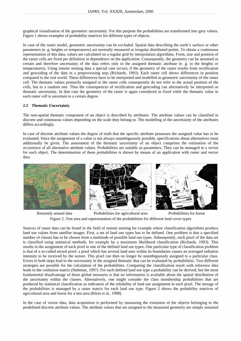
graphical visualisation of the geometric uncertainty. For this purpose the probabilities are transformed into grey values.Figure 1 shows examples of probability matrices for different types of objects.

In case of the raster model, geometric uncertainty can be excluded. Spatial data describing the earth’s surface or otherparameters (e. g. heights or temperatures) are normally measured at irregular distributed points. To obtain a continuousrepresentation of this data, values are calculated on a regular grid by interpolation algorithms. Form, size and position ofthe raster cells are fixed per definition in dependence on the application. Consequently, the geometry can be assumed ascertain and therefore uncertainty of the data refers only to the assigned thematic attribute (e. g. in the heights ortemperatures). Using remote sensing data a special case occurs, if the geometry of the raster results from rectificationand geocoding of the data in a preprocessing step (Richards, 1993). Each raster cell shows differences in positioncompared to the real world. These differences have to be interpreted and modelled as geometric uncertainty of the rastercell. The thematic values primarily assigned to the raster cells consequently do not refer to the actual position of thecells, but to a random one. Thus the consequences of rectification and geocoding can alternatively be interpreted asthematic uncertainty. In that case the geometry of the raster is again considered as fixed while the thematic value ineach raster cell is uncertain to a certain degree.

2.2 Thematic Uncertainty

The non-spatial thematic component of an object is described by attributes. The attribute values can be classified indiscrete and continuous values depending on the scale they belong to. The modelling of the uncertainty of the attributesdiffers accordingly.

In case of discrete attribute values the degree of truth that the specific attribute possesses the assigned value has to beevaluated. Since the assignment of a value is not always unambiguously possible, specifications about alternatives mustadditionally be given. The assessment of the thematic uncertainty of an object comprises the estimation of theoccurrence of all alternative attribute values. Probabilities are suitable as parameters. They can be managed in a vectorfor each object. The determination of these probabilities is shown by means of an application with raster and vectordata.

Remotely sensed data Probabilities for agricultural area Probabilities for forestFigure 2. Test area and representation of the probabilities for different land cover types

Sources of raster data can be found in the field of remote sensing for example where classification algorithms produceland use values from satellite images. First, a set of land use types has to be defined. One problem is that a specifiednumber of classes has to be chosen from a multitude of possible land use types. Subsequently, each pixel of the data setis classified using statistical methods, for example by a maximum likelihood classification (Richards, 1993). Thisresults in the assignment of each pixel to one of the defined land use types. One particular type of classification problemis that of a so-called mixed pixel: a pixel which has several land uses within its boundaries causes an averaged radiationintensity to be received by the sensor. This pixel can then no longer be unambiguously assigned to a particular class.Errors in both steps lead to the uncertainty in the assigned thematic that can be evaluated by probabilities. Two differentstrategies are possible for the calculation of the probabilities. Comparing the classification result with reference dataleads to the confusion matrix (Stehman, 1997). For each defined land use type a probability can be derived, but the mostfundamental disadvantage of these global measures is that no information is available about the spatial distribution ofthe uncertainty within the classes. Alternatively, one might consider the class membership probabilities that areproduced by statistical classification as indicators of the reliability of land use assignment in each pixel. The storage ofthe probabilities is managed by a raster matrix for each land use type. Figure 2 shows the probability matrices ofagricultural area and forest for a test area (Klein et al., 1998).

In the case of vector data, data acquisition is performed by measuring the extension of the objects belonging to thepredefined discrete attribute values. The attribute values that are assigned to the measured geometry are simply assumed

IAPRS, Vol. XXXIII, Amsterdam, 2000

to contain no uncertainties. In reality this restriction is not always warrantable since the acquired objects can beinhomogeneous with regard to the thematic aspects or the assignment of the attributes can be uncertain. For a completemodelling of thematic uncertainty the percentage of the respective attributes, that can be interpreted as probabilities,should be specified.

In connection with thematic uncertainty, it is furthermore important to extend the uncertainty description to continuousattribute values so that e. g. heights or temperatures can be qualified. Also these data contain a certain degree ofuncertainty since they are derived from measurements. The variation of the attribute value characterises the thematicuncertainty. Analogous to the geometric uncertainty a stochastic approach can be chosen to model the continuousattribute values as random variables. Then the variation of the attribute value is represented by mean value andvariance. Thematic data existing in irregular distributed points are normally converted to a regular grid. For thispurpose, it is important to determine the variances of the interpolated values by statistical methods, too. The storage ofthe interpolated values and their variances can again be managed by matrices i. e. as raster data (section 4.1).

3 HYBRID DATA MODEL INTEGRATING DATA UNCERTAINTY

A hybrid data model (Glemser and Fritsch, 1998) builds the basis for the integration of the uncertainty. The approachrests upon objects as exclusive representations of spatial phenomena. As a consequence, an object building procedure

has to be applied in some casesbefore the data can be integrated(Klein et al., 1998). The geometriccomponent allows either a raster or avector representation of the object.Such a hybrid model enables the userto process data without ever noticingwhether the actual type is raster orvector. In the thematic componentmultiple attributes of any kind areattached to the object. Attributevalues can be distinguished accord-ing to the scale they belong to.Figure 3 shows on the left side a

schematic graphical representation of the hybrid data model in UML syntax (Booch et al., 1999). Since both thegeometry and the thematic of an object can be uncertain, the hybrid data model has to be extended by a description ofthe uncertainty. As already explained, probabilities and standard deviations can be utilised. Since they are used similarlyfor the description of uncertainty in the geometric component, they can be seen as alternative possibilities. But in thethematic component they are used independent from each other. The uncertainty of discrete attribute values is describedby probabilities, the uncertainty of continuous attribute values by standard deviations. If it is possible to assignalternative attributes to an object, each attribute requires its own uncertainty description. Thus the description of anobject could comprise e. g. one probability raster for the geometric uncertainty and several measures for the thematicuncertainty of its attributes. Figure 3 shows the defined uncertainty model on the right side as an extension of the initialhybrid model.

4 COMPLEX ANALYSIS

Since all data only have a limited accuracy it is important for the user to know how the result of the analysis can beassessed with respect to its accuracy. This problem can only be adequately solved if the uncertainty of the input datasets is inserted in the analysis process and propagated onto the result. As an example application, the forecast of thespatial extent of a possible flooding of a river is selected. The special task to be solved is to detect those parts ofsettlement areas which are flooded with respect to an assumed high water level. It defines a complex problem in theway that the whole process consists of two successive steps. In the first step a flooding model has to be developed. Inthe second step, the derived outcome is geometrically overlaid with topographic information, namely the settlementareas. The major goal is to determine the uncertainty of the result in addition to the traditional output without regard ofdata uncertainty.

objectgeometry

thematic

11

10..*

raster vector

discrete continuous

nominal ordinal interval ratio

uncertaintyprobabilities

standard deviation

1

1

0..1

0..1

Figure 3. Hybrid data model integrating the uncertainty model

IAPRS, Vol. XXXIII, Amsterdam, 2000

4.1 Data Sets

Basically, the analysis requires different input data sets. The topographic surface strongly influences which areas areflooded. It can be described by a digital terrain model (DTM). As source of the flood, the location of the river is neededas well as the location of the settlement areas which might be affected by the flood. The necessary land use informationcan be taken from a topographic data set.

a) b)

204 213 223 232 242 251 261 271 280 290 300 309 319 1.0 m 2.0 m

Figure 4. Digital terrain model (a) and its uncertainty given by variances of the heights (b)

The DTM for the study area is shown in figure 4a. The heights are structured in a regular grid and therefore they form araster data set with a ground pixel size of 5m. Each raster cell carries a height value as an attribute belonging to thecontinuous scale. For the representation of the uncertainty a variance for each raster cell is required. In principle theaccuracy of the originally measured values has to be transformed to raster data. Since this information is only availablesparsely, often qualified models are formulated. A simple approach would be to assume the same height variance foreach cell. A more complex determination is based on the dependency of the variance on the slope. In this application aslope dependent approach is chosen (figure 4 b). The accuracy of the heights varies between 1m and 2m.

a) b)

river settlement forest agriculture0.0 0.1 0.2 0.3 0.4 0.5 0.6 0.7 0.8 0.9 1.0

Figure 5. Land use data (a) and the graphical representation of the probabilities of the settlement data set (b)

The land use data set (figure 5a) is extracted from an existing digital topographic database, called ATKIS, which is theGerman topographic cartographic spatial database (ATKIS, 1997). The database defines a digital model of the physicallandscape. The relevant contents of the landscape are modelled as objects which are successively aggregated to objectclasses (e. g. roads), object groups (e. g. road transportation) and finally to object domains (e. g. transportation). Thescale is 1:25.000. All data is collected in vector format with a positional accuracy of 3m for important objects (e. g.roads, railways, rivers) and a reduced accuracy of 10m for all others. For the flooding analysis two object classes arerelevant: stream and residential area. The study area contains one stream object (the river Enz) and five residential areasthat build together the settlement area of interest. For visualisation of the uncertainty and implementation of theanalysis, the description in terms of variances of the settlement areas is transformed to a representation in terms ofprobabilities (figure 5b). The probabilities indicate the degree of membership to the object.

IAPRS, Vol. XXXIII, Amsterdam, 2000

4.2 Thematic Analysis

The determination of the flooded area requires the formulation of a flood model. For each raster cell of the river it isexamined how the increasing water-level affects the neighbouring raster cells. Thus, an individual flooded area isdetermined for each river cell and the overlay of these partial areas results in the complete area. The result of theforecast of the flooding is presented in figure 6a. Since the DTM only has a limited accuracy it is important to knowhow the result of the flooding can be assessed with respect to accuracy. A major difficulty is that the functional contextbetween the digital elevation model and the flooded region can only be modelled in a complex way. Thus, the variancepropagation based on a functional context is not suitable to determine the uncertainty description of the flooded area.Simulation techniques are used alternatively to solve the problem.

a) b)

settlement area river flooded area0.0 0.1 0.2 0.3 0.4 0.5 0.6 0.7 0.8 0.9 1.0

Figure 6. Outcome of the simulated flooding (a) and the representation of the probabilities of the flood region (b)

Simulation can be described as generation of realisations of a mathematical system by variation of the input variables(Piehler and Zschiesche, 1976). If stochastic data are used, simulation is called stochastic as well. In the presentapplication this concerns the generation of the flooded region due to the stochastic behaviour of the elevation model.The problem can be solved by using Monte Carlo methods (Sobol, 1985). Monte Carlo methods are special proceduresfor the simulation of stochastic problems generating random samples by random numbers. The stochastic behaviour ofthe samples results from a predefined probability density function. For a given stochastic input variable, the outcomesof the simulation are the realisations of a random variable. The digital elevation model builds the basis of the simulationconsidering the heights as random variables. Assuming a Gaussian or Normal distribution, the heights are describedsufficiently by height value and variance.

The determination of the uncertainty of the flooded region is achieved as follows: in a first step n realisations of theelevation model are generated using the probability density function for each height. Then, according to the formulatedflood model, the spatial extent of a possible flooding is determined for each of the n realisations. The outcome of thesimulation are n different and independent realisations of the flooded region. For a representative conclusion from thesample to the population the volume n of the sample has to be large enough (e. g. n = 1000). The quality of the derivedstatement about the uncertainty of the flooded area depends primarily on the volume of the sample. The morerealisations are produced, the more reliable is the result - but computing effort increases at the same time.

For the analysis of the simulation, the n flooded regions are overlaid and for every raster cell the frequency of floodingis determined. Frequency can be interpreted as probability which indicates the membership of the cell to the object´flooded region´. The complete probability matrix can be considered as outcome of the simulation. Grouping all cellswith probabilities larger than 0.0 results in the maximum extent of the flooded area (figure 6b).

Concerning the integration of uncertainty, the simulation result covers a larger area in comparison with the traditionalsolution. Not only a modified extension is derived, but also the probability of a flooding is spatially quantified. Thegraphical representation of the probabilities shows clearly that the uncertainty of the heights causes the uncertainty ofthe boundary, namely the spatial extent of the flooded area.

4.3 Geometric Analysis

In the next step the flooded area is geometrically overlaid with the settlement areas. The result is a set of new objectsconsisting only of the intersection parts but possessing attributes of all the input objects. It is easier to implement theoverlay operation with raster data than with vector data. In the raster domain it is a simple boolean And-operator on the

IAPRS, Vol. XXXIII, Amsterdam, 2000

raster cells, while in the vector domain the computation of points of intersection is very time-consuming. To takeadvantage of this fact in hybrid systems, polygon overlay is realised using raster overlay techniques. Therefore, thesettlement areas given in vector format have to be transformed to objects in raster format by a vector-to-rasterconversion. The realisation of a hybrid GIS requires that the conversions run automatically as a kind of backgroundoperation without any user interaction, even without being noticed by the user (Fritsch et al., 1998).

a) b)

flooded settlement area0.0 0.1 0.2 0.3 0.4 0.5 0.6 0.7 0.8 0.9 1.0

Figure 7. Flooded settlement area (a) and the representation of the probabilities of the flooded settlement area (b)

The outcome of the overlay is shown in figure 7a. The shapes of the five resulting objects can be divided into areas andlines. For a better identification, the regions with the three line objects are shown in an enlarged inset of the orthophoto.The line objects appear when settlement areas and flooded region touch or have only a very small overlay. With respectto the result of the conventional overlay analysis such sliver polygons are considered as irrelevant and removed fromthe database. However, it is doubtful if doing so is warrantable. Since all data is uncertain to a certain degree, the spatialextension of the objects respectively their boundary is to be considered to be uncertain, too. To obtain reliable resultsfor the analysis the uncertainty of the objects needs to be modelled and integrated in overlay. Since the overlayoperation can be interpreted as a simple boolean And-operator, the propagation of the probabilities is defined by

1 2 1 2( ) ( ) ( )p A A p A p A∩ = ⋅ .

1( )p A and 2( )p A denote the probabilities of the two raster cells possessing the assigned attribute values 1A and 2A ,

in this case settlement area and flooded area.

The comparison of figure 7b with figure 7a shows that the integration of the uncertainty results in a larger endangeredarea. Therefore the sliver polygons can no longer be considered as irrelevant. They should be removed from thedatabase only after analysing their probabilities. Disregarding the uncertainty leads to a misinterpretation of the results.This example application shows clearly that it is important to integrate the uncertainty in data processing as well as toinclude the uncertainty into the visualisation of the results.

5 CONCLUSIONS

The paper focuses on the extension of a hybrid data model by an uncertainty model. Since both the geometry and thethematic of an object can be uncertain, description of uncertainty has to be taken into account in both components.Probabilities and standard deviations are utilised as parameters for the uncertainty. The developed model establishes thebasis for the integration of uncertainty in interoperable applications. An example shows in a demonstrative way whichmodifications become necessary and how results of analysis are to be interpreted with respect to their uncertainty.During analysis processes, either typical mathematical error propagation methods perform the estimation of therequested uncertainty or simulation techniques are utilised for complex applications. But it is not sufficient to considerdata uncertainty only in individual analysis methods. In fact all available functions must provide appropriate extensions.A second source of uncertainty can be detected in the analysis model applied. A decisive characteristic of a model isthat it defines only a kind of approximation of the reality. For example, the used flooding model does not correspondexactly to the real situation of a flooding because of the complexity of the process itself. This aspect has not beencovered so far.

IAPRS, Vol. XXXIII, Amsterdam, 2000

ACKNOWLEDGMENTS

This research work is founded by the German Research Foundation (DFG) within the joint project IOGIS (InteroperableOffene Geowissenschaftliche Informationssysteme).

REFERENCES

ATKIS, 1997. Amtlich Topographisches-Kartographisches Informationssystem (ATKIS). Arbeitsgemeinschaft derVermessungsverwaltungen der Länder der Bundesrepublik Deutschland (AdV). http://www.atkis.de.

Bill, R., Fritsch, D., 1991. Grundlagen der Geo-Informationssysteme. Band 1: Hardware, Software und Daten. Wich-mann, Karlsruhe.

Bill, R., Korduan, P., 1998. Flächenverschneidung in GIS – Stochastische Modellierung und Effizienzbetrachtung. Zeit-schrift für Vermessungswesen, Vol. 123, Part 1 in No. 8, pp.247-253, Part 2 in No. 10, pp.333-338.

Booch, G., Rumbaugh, J., Jacobson, I., 1999. The Unified Modelling Language User Guide. Addison-Wesley.

Fritsch, D., Glemser, M., Klein, U., Sester, M., Strunz, G. (1998): Zur Integration von Unsicherheit bei Vektor- undRasterdaten. GIS, Vol. 11, No. 4, pp.26-.35

Glemser, M., Fritsch, D., 1998. Data Uncertainty in a Hybrid GIS. In: Fritsch, D., Englich, M., Sester, M.: GIS –Between Visions and Applications, IAPRS, Vol. 32, Part 4, Stuttgart, Germany, pp.180-187.

Glemser, M., Klein, U., 1999. Hybride Modellierung und Analyse von unsicheren Daten. Schriftenreihe der Institutedes Fachbereichs Vermessungswesen, Universität Stuttgart, Report No. 1999.1, pp.27-43.

IOGIS, 1999. Interoperable Offene Geowissenschaftliche Informationssysteme (IOGIS).http:\\ifgi.uni-muenster.de/3_projekte/4dgis/texte/iogis/IOGIS.html.Klein, U., Sester, M., Strunz, G., 1998. Segmentation of Remotely Sensed Images Based on the Uncertainty of Multi-spectral Classification. In: IAPRS, Vol. 32, Part 4, Stuttgart, Germany, pp.299-305.

Kraus, K., Haussteiner, K., 1993. Visualisierung der Genauigkeit geometrischer Daten. GIS, Vol. 6, No. 3, pp.7-12.

McKee, L., Kuhn, W., 1997. The OpenGIS Consortium’s Purpose and Technical Approach. In: Fritsch D., Hobbie, D.(Eds.): Photogrammetric Week ’97, Wichmann, Heidelberg, pp.237-242.

OGC, 1999. Open GIS Consortium (OGC). http://www.opengis.org.

Piehler, J., Zschiesche, H.-U., 1976. Simulationsmethoden. Mathematik für Ingenieure, Band 20. Teubner Verlag,Leipzig.

Richards, J. A., 1993. Remote Sensing Digital Image Analysis. Springer-Verlag.

Sobol, I. M., 1985. Die Monte-Carlo-Methode. Deutsche Taschenbücher, Band 41, Verlag Harri Deutsch, Thun undFrankfurt am Main.

Stehman, S. V., 1997. Selecting and Interpreting Measures of Thematic Classification Accuracy. Remote Sensing of theEnvironment, Vol. 62, pp.77-89.