Embed Size (px)
Citation preview

HAL Id: hal-02331028https://hal.archives-ouvertes.fr/hal-02331028
Submitted on 24 Oct 2019
HAL is a multi-disciplinary open accessarchive for the deposit and dissemination of sci-entific research documents, whether they are pub-lished or not. The documents may come fromteaching and research institutions in France orabroad, or from public or private research centers.
L’archive ouverte pluridisciplinaire HAL, estdestinée au dépôt et à la diffusion de documentsscientifiques de niveau recherche, publiés ou non,émanant des établissements d’enseignement et derecherche français ou étrangers, des laboratoirespublics ou privés.
Hybrid system combining mechanical compression andthermochemical storage of ammonia vapor for cold
productionJaume Fitó, Alberto Coronas, Sylvain Mauran, Nathalie Mazet, Maxime
Perier-Muzet, Driss Stitou
To cite this version:Jaume Fitó, Alberto Coronas, Sylvain Mauran, Nathalie Mazet, Maxime Perier-Muzet, et al..Hybrid system combining mechanical compression and thermochemical storage of ammonia va-por for cold production. Energy Conversion and Management, Elsevier, 2019, 180, pp.709 - 723.�10.1016/j.enconman.2018.11.019�. �hal-02331028�
Energy Conversion and Management Volume 180, 15 January 2019, Pages 709-723
1
Hybrid system combining mechanical compression and thermochemical storage 1
of ammonia vapor for cold production 2
Jaume Fitóa,b,c, Alberto Coronasc, Sylvain Maurana,b, Nathalie Mazeta, Maxime Perier-Muzeta,b,*, Driss Stitoua 3
a CNRS-PROMES Laboratoire Procédés Matériaux et Energie Solaire UPR 8521, Perpignan 66100, France 4
b Université de Perpignan Via Domitia (UPVD), Perpignan 66860, France 5
c Department of Mechanical Engineering, Universitat Rovira i Virgili, Tarragona 43007, Spain 6
* Corresponding author. E-mail address: [email protected]. 7
8
A B S T R A C T 9
This paper studies a hybrid system for cold production consisting of a compression cycle combined with a thermochemical process 10
by sharing the same condenser, evaporator and refrigerant fluid. The aim of this hybridization is to solve mismatch issues between 11
the demand of cold and the source of energy (availability and/or price) with a system as compact as possible. One important side 12
benefit is that the interaction between the compressor and the thermochemical reactor reduces the activation temperature for 13
ammonia desorption in the thermochemical reactor. To study this interaction a quasi-steady simulation model for both storage 14
and de-storage phases has been developed and experimentally validated by means of a small scale (approx. 300 Wh of cold 15
storage) experimental bench with ammonia as refrigerant and barium chloride (BaCl2) as reactant salt. Experiments proved a 35 16
K reduction in the activation temperature of the desorption reaction with respect to desorption without compressor. Model 17
validation by adjusting permeability and thermal conductivity of the reactive composite showed an acceptable agreement between 18
predicted and experimental reaction advancement-time curves. The validated model was used for simulation of the system in a 19
preliminary case study, representative in power (40 kW) and temperature (-25°C) of an industrial cold demand. It is shown that 20
during ammonia de-storage, the hybrid achieves a higher COP than a conventional mechanical vapor compression system. It 21
increases exponentially with the relative share of thermochemical storage in the cold production. 22
Keywords: Refrigeration, Hybrid system, Vapor compression refrigeration, Thermochemical storage, Low-grade heat source, 23
Heat and mass transfer. 24
H I G H L I G H T S 25
Compression-thermochemical cooling system with electricity & low-grade heat input. 26
35 K heat source temperature reduction through compression-assisted desorption. 27
Quasi-steady simulation model validated accounting for heat and mass transfers. 28
Preliminary case study with bi-stage compression and cold production at -25 ºC. 29
2 times higher COP than vapor compression during ammonia de-storage phase. 30
Energy Conversion and Management Volume 180, 15 January 2019, Pages 709-723
2
Nomenclature
Names and variables Greek symbols
G Gas Increment
h Specific enthalpy, kJ·kg-1or kJ·mol-1 Fraction of cold produced by the thermochemical subsystem
during synthesis phase
k Permeability, m2 Efficiency
M Molar mass, kg·kmol-1 Effective thermal conductivity, W·m-1·K-1
m Mass, kg Dynamic viscosity, Pa·s
�̇� Mass flow rate, kg·s-1 Density, kg·m-3
�̇� Mole flow rate, mol·s-1 �̃� Apparent density, kg·m-3
P Pressure, bar Compression ratio
�̇� Heat power, kW Reaction’s stoichiometric coefficient, mole-gas·mole-salt-1
Q Heat, kWh COP ratio between hybrid system and MVC system
R Thermochemical Reactor Moles of refrigerant in the fully discharged salt
ℜ Ideal gas constant, J·mol-1·K-1
r Radius, m Subscripts and Superscripts
S Solid
s Specific entropy, J·kg-1·K-1or J·mol-1·K-1 º Reference point
T Temperature, ºC 0 Fully discharged reactive salt (X = 0)
t Time, h 1 Fully charged reactive salt (X = 1)
Uw Global heat transfer coefficient, W·m-2·K-1 c Constraint temperature or pressure applied to the reactor
V Volume, m3 cd Condenser
�̇� Volumetric flow rate, m3·s-1 dec Decomposition phase
v Specific volume, m3·kg-1 d Gas diffuser
�̇� Power, kW ev Evaporator
W Work, kWh eq Equilibrium
w Mass fraction, kg·kg-1 f1 Mass transfer-limited reaction front
X Reaction advancement degree (-) f2 Heat transfer-limited reaction front
Z Axial coordinate and length of reactive composite, m h High temperature or pressure level
HP Relative to High-Pressure compressor
Acronyms HYB Hybrid system
i Inlet
CAD Compression-Assisted Decomposition l Low temperature or pressure level
COP Coefficient Of Performance LP Relative to Low-Pressure compressor
D# Decomposition reaction experiment (# goes from 1 to 3) m Medium temperature or pressure level
Dec Energy storage density of the reactive composite, kWh-heat /
m3-composite (based on heat of reaction)
min Minimum
ENG Expanded Natural Graphite MVC Mechanical Vapor Compression
EV Expansion Valve o Outlet
HCTRS Hybrid Compression-Thermochemical Refrigeration System r Reaction, reactor, or reactive composite

Energy Conversion and Management Volume 180, 15 January 2019, Pages 709-723
3
L/V Liquid / Vapor rd Decomposition reaction
MVC Mechanical Vapor Compression rs Synthesis reaction
MX Metal halide s Isentropic
S# Synthesis phase experiment (# goes from 1 to 3) sa Anhydrous reactive salt
TCH Thermochemical syn Synthesis phase
TOD Thermally-Only activated Decomposition syn-dec Complete TCH cycle (synthesis and decomposition)
V-XX Valve number XX (goes from 01 to 16) TCH Thermochemical
w Reactor’s wall
1. Introduction 31
The current need to reduce GHG emissions and decarbonize energy systems has increased the interest of using 32
renewable sources and recovering low-grade waste heat in the recent decades [1]. The impact of cold production in 33
the commercial sector is not negligible: for instance, supermarkets and hypermarkets represent 56 % of the total 34
demand of cold in France’s commercial sector [2]. Compression refrigeration is a mature technology, and if applied 35
for solar operation, it can also benefit from the competitive costs of solar photovoltaic (PV) technology [3]. A classic 36
problem is the mismatch between the solar resource and the cold demand [4,5]. If this mismatch is solved by having 37
the system connected to the grid, it happens that the price of this source is variable, thus creating another type of 38
mismatch (cold demand/source price). An answer to the problem of mismatch is energy storage, to store surplus cold 39
during favorable periods (sunshine hours or low price of the source) for later use [6]. One idea is placing phase 40
change materials (PCM) in the cold delivery unit, which has been studied experimentally for solar-PV compression 41
refrigeration driven with DC motor [7]. Otherwise, the storage can be placed outside of the unit, as studied 42
experimentally for solar-PV air conditioning with ice thermal storage [8], for instance, or the energy can be stored by 43
means of batteries [9]. 44
Thermochemical processes allow mid- and long-term energy storage with nearly negligible heat losses [10], for 45
several applications such as solar air conditioning [11], cooling + heating [12], or long-term storage of solar energy 46
[13]. Another interesting application proposed is deep-freezing [14], by means of a cascading process that has the 47
added benefit of being driven by low-grade heat. Indeed, thermochemical systems can utilize low-grade to mid-grade 48
heat sources depending on the choice of reactive pair [15], and usually, several useful effects can be obtained from 49
these systems, such as cascaded use and storage of solar thermal energy [16], especially when they are configured 50
with two reactive beds [17,18]. Several of the systems in these studies are ammonia-based [19]. The idea of replacing 51
the condenser/evaporator with a secondary adsorbent reactor has also been investigated, under the name of 52
resorption [20]. The notable advantages of thermochemical processes can make these processes economically 53

Energy Conversion and Management Volume 180, 15 January 2019, Pages 709-723
4
competitive in the near future. The idea of combining the maturity of vapor compression with the prospective 54
competitiveness of thermochemical storage seems promising. 55
The coupling of absorption or desorption processes with mechanical vapor expansion or compression was 56
patented by Moritz Honigmann in 1883 [21]. Recently, the so-called ‘Honigmann process’ was re-evaluated by 57
Jahnke et al. [22] as thermochemical storage producing power during desorption phase, and later simulated for the 58
LiBr/H2O and NaOH/H2O working pairs [23]. Bao et al. developed the idea of combining thermochemical processes 59
with vapor compression [24] and with vapor expansion [25]. The concepts were presented under the name of 60
‘integrated chemisorption cycles’, and the suggested applications were ultra-low grade (30 ºC – 100 ºC) heat recovery 61
and thermo-electric energy storage. The study considered ammonia as working fluid and manganese chloride 62
(MnCl2), calcium chloride (CaCl2) and sodium bromide (NaBr) as reactant salts. The coupling between the reactor 63
and the compressor is reported to show some instabilities because of the variable flow rate of ammonia entering the 64
compressor, and one solution proposed for similar systems (expansion/thermochemical) is to place a buffer tank at 65
the reactor outlet to reach constant inlet rate of ammonia [26,27]. Recently, Ferruci et al. [28] pursued the concept of 66
thermochemical storage driven by mechanical vapor compression activated by solar-PV energy. The system was 67
proposed with ammonia as refrigerant and barium chloride (BaCl2) as reactant salt for cooling applications, 68
highlighting as main strengths the thermochemical storage and the possibility of using low-temperature heat sources 69
thanks to the compressor aiding the desorption of ammonia in the reactor. 70
Further studies on this hybrid thermochemical/compression system are not abundant, although several 71
experimental studies exist with thermochemical systems alone, especially with the NH3/BaCl2 reaction, and 72
mechanical vapor compression refrigeration is a mature technology. In addition, other concepts very similar to 73
hybridization have been proposed, for instance an adsorption/compression cascade system [29]. The idea of coupling 74
mechanical vapor compression with thermochemical storage can result in interesting hybrid systems with high 75
potential for waste heat utilization, and their experimental study is feasible. 76
This paper investigates further into this idea and studies experimentally an ammonia-based refrigeration system 77
consisting in the hybridization of compression refrigeration with thermochemical storage implementing the NH3/BaCl2 78
pair [30]. The main novelties of this paper with respect to literature are the approach chosen for simulation as well as 79
the experimental validation. The system utilizes low-grade heat thanks to its compression-assisted reduction of 80
activation temperature (described in Section 2), and benefits from the advantages of thermochemical storage. The 81
absorption, desorption, and compression-assisted desorption stages are simulated by means of a quasi-steady dual-82
front model (Section 3). An experimental bench was built to validate the model by adjusting composite’s permeability 83

Energy Conversion and Management Volume 180, 15 January 2019, Pages 709-723
5
and thermal conductivity, the most representative parameters of mass and heat transfer respectively (Section 4). 84
Experimental results show a 35 K reduction in heat source temperature thanks to the compression-assisted 85
desorption. The validated model is then used for simulation in a simplified case study (Section 5) of a different 86
configuration of the hybrid system operating at different conditions with the NH3/SrCl2 and the NH3/CaCl2 pairs. This 87
preliminary case study is offered for a permanent production of 40 kW cold at -25 ºC which is representative of the 88
needs for cold stores of supermarkets. 89
2. System description 90
Figure 1 depicts the operating principle of the hybrid compression-thermochemical refrigeration system (HCTRS) 91
on a simplified Clausius-Clapeyron diagram. The vapor/liquid equilibrium of pure refrigerant is represented with a 92
green line, and the red line represents a reversible solid/gas thermochemical reaction. The HCTRS consists of two 93
subsystems: the mechanical vapor compression (MVC) subsystem, made up of a compressor, a condenser, an 94
expansion valve and an evaporator; and the thermochemical (TCH) subsystem, made up of a thermochemical 95
reactor, the condenser, a storage tank, the expansion valve and the evaporator. The hybridization consists of the 96
same condenser, expansion valve, evaporator and refrigerant fluid being shared by both subsystems. The HCTRS 97
requires an input of both electric and thermal energy and operates within 3 temperature levels and at least 2 pressure 98
levels. Indeed, each subsystem can be operated separately from the other, but for the sake of simplicity, Fig. 1 99
focuses only on the three most characteristic operating modes. 100
Fig. 1a: Simultaneous production of
cold with the thermochemical
subsystem (synthesis phase) and
with the mechanical vapor
compression subsystem, depicted
in the Clausius-Clapeyron diagram.
Fig. 1b: Cold production by the
mechanical vapor compression
subsystem with simultaneous storage
of refrigerant by the thermochemical
subsystem activated by thermal
source only (classic decomposition
phase) at condenser pressure.
Fig. 1c: Cold production by
mechanical vapor compression and
simultaneous thermochemical storage
of refrigerant activated by low-grade
thermal energy at P < Ph, thanks to the
compressor (compression-assisted
decomposition).
Energy Conversion and Management Volume 180, 15 January 2019, Pages 709-723
6
The first one is simultaneous cold production by the MVC and the TCH (Fig. 1a). Stored refrigerant from the TCH 101
is released into the evaporator and provides additional cold production. This can be used to assist the MVC in periods 102
of peak demand with unstable electric source, or to reduce its load in the case of a stable electric source but with 103
higher price. Thanks to the thermochemical process, the energy storage saves one step of energy conversion during 104
the discharge stage, reducing the inertia of the system in comparison with electricity storage in batteries. Refrigerant 105
vapor leaving the evaporator is divided into two streams: one enters the compressor for the MVC cycle, and the other 106
reacts with the salt inside the TCH reactor, in an exothermic process with the reaction heat released at ambient 107
temperature. 108
The second characteristic mode of the hybrid system is the possibility of producing cold by MVC while storing 109
ammonia with the TCH activated with a heat source (Fig. 1b). Both ammonia streams leaving the compressor and 110
the reactor join before entering the condenser. The part corresponding to TCH storage is kept in a tank right after 111
condensing. This mode will be hereinafter called ‘Thermally-Only activated Decomposition’ (TOD) in this study. In 112
TOD, activation temperatures can be relatively high depending on reactive pair and condenser pressure. This may 113
force to discard certain heat sources that do not have enough temperature, as sometimes happens with classical 114
TCH systems because of their monovariant equilibrium. Nevertheless, in the HCTRS the reactor and compressor 115
can be connected to facilitate decomposition reactions at pressures lower than the condenser pressure, and therefore 116
lower activation temperatures. 117
The third and most interesting operating mode, ‘Compression-Assisted Decomposition’ (CAD, Fig. 1c), makes 118
this connection possible. The compressor allows the reactor pressure to be different from the condenser pressure, 119
granting an additional degree of freedom. This allows decomposition at low pressure (Pl) simultaneously to MVC cold 120
production. Of course, operating pressure can be adjusted to any value between Pl and Ph (it could be regarded as 121
a ‘floating’ pressure level), to utilize any waste heat at the required temperature level for this suction pressure. This 122
possibility can be investigated until process activation at ambient temperature: this case may well imply reactor 123
pressures even lower than the low pressure level itself. The CAD enables low-grade waste heat recovery, as well as 124
selection of well-performant reactive pairs (such as ammonia-barium chloride) despite heat source temperatures 125
below reaction equilibrium temperature at condenser pressure. 126
The reversible solid/gas thermochemical reaction is usually written as in eq. (1). <MX> is a metallic salt reacting 127
between and ( + ) moles of refrigerant gas (G), is the stoichiometric coefficient and ∆hrº is the standard enthalpy 128
of reaction. The equilibrium formed by G, <MX·G> and <MX·( +)G> is monovariant and represented by eq. (2), 129

Energy Conversion and Management Volume 180, 15 January 2019, Pages 709-723
7
where values of ∆ℎ𝑟0 and ∆𝑠𝑟
0 referred by mole of gas (ammonia) are given by Touzain [31] for each reactive pair and 130
assumed constant with respect to temperature. The reference pressure P0 is 1 bar. 131
⟨𝑀𝑋 · 𝜉𝐺⟩ + 𝜈(𝐺) ⇌ ⟨𝑀𝑋 · (𝜉 + 𝜈)𝐺⟩ + 𝜈 · ∆hr° (1) 132
ln (𝑃𝑒𝑞
𝑃° ) =−∆ℎ𝑟
°
ℜ·𝑇𝑒𝑞,𝑟+
∆𝑠𝑟°
ℜ (2) 133
3. Modeling 134
The sizing of the two essential components of the HCTRS hybrid system, namely the compressor and the reactor, 135
depends mainly on the temperatures of the heat sources and sinks (in particular the one to which the cold is 136
delivered), the desired cooling power and the scenario of storage and restitution, i.e. the energies and respective 137
powers provided by the two subsystems MCV and TCH. For common applications, such as the one discussed in 138
Section 5, the sizing of the compressor is straightforward (issue from suppliers' catalogs). It must be able to aspirate 139
the sum of both ammonia flow rates coming from evaporator and reactor in CAD phase. 140
On the other hand, the design of the reactor is not so obvious. Indeed the running of the solid / gas reactor is 141
intrinsically unsteady, with instantaneous power decreasing overall between the beginning and the end of the 142
reaction, both in synthesis and in decomposition phases, and even when the thermodynamic constraints (T and P) 143
applied to the reactor are kept stable. The modeling of this hybrid system is therefore more complex, and even more 144
so when the reactor is coupled to the compressor during the CAD phases, given the antagonistic contributions of the 145
compressor and the reactor that affect the reactor pressure: the decomposition reaction releases refrigerant gas 146
(thus contributing to pressure increase) while the compressor removes it (thus contributing to pressure decrease). 147
In all cases, including purely thermal decompositions (TOD), reactor modeling is necessary to estimate the 148
performance of HCTRS systems with different solid / gas reactions, thermodynamic constraints and reactor sizes. 149
This modeling, detailed below, allowed to firstly dimension an experimental bench of a HCTRS system with a small 150
power, and secondly to fit with sufficient precision the parameters of the model on a whole series of experiments. 151
3.1. Model’s hypotheses 152
There are several more or less sophisticated models able to describe solid / gas reaction rate as a function of the 153
implementation of the reagent, the applied thermodynamic constraints (Tc, Pc) and the geometry of the inner heat 154
exchanger and gas diffuser. The most accurate [32] is based on the resolution of a system coupling the equation of 155
heat and that of mass conservation, including the terms of accumulation (i.e. sensible heat and variation of mass of 156

Energy Conversion and Management Volume 180, 15 January 2019, Pages 709-723
8
gas in the porous volume). In this model, the gas flow rates and the reaction heat fluxes are connected by a kinetic 157
law of transformation of the reactive grain, which is a function of a local deviation from the thermodynamic equilibrium. 158
On the other hand, the simplest model [33] assumes a uniform and constant temperature of the reactant during the 159
reaction and a reaction rate solely as a function of an overall coefficient of heat exchange between the reactive solid 160
and the coolant. The model used here is of intermediate complexity; it neglects the terms of accumulation and 161
therefore does not adequately reflect evolutions in the temperature and pressure profiles within the reactive fixed 162
bed. On the other hand, it correctly accounts for reactor power evolutions that are more useful for quantifying the 163
performance of an HCTRS system. 164
The model is constructed for a reactive medium with a cylindrical geometry (Fig. 2) and calculations are carried 165
out in the radial direction. Refrigerant gas (assumed as a perfect gas) at the constraint pressure Pc leaves or enters 166
the cylindrical reactor through a gas diffuser in its axis, and the constraint temperature Tc is applied via a heat transfer 167
fluid circulating through an external coil exchanger at the peripheral wall. The advancement degree of the reaction is 168
bound to limitations of heat transfer and mass transfer, and the model takes both into account. 169
Fig. 2: Schematic view of the thermochemical reactor.
During synthesis, dark grey area represents salt that
already reacted and light grey area corresponds to salt that
is yet to react, and vice versa during decomposition phase.
The yellow (at rf2) and grey (at rf1) boundaries are the two
fronts of reaction.

Energy Conversion and Management Volume 180, 15 January 2019, Pages 709-723
9
The main hypothesis of this model (also detailed in [32,34]) is the existence of two ‘sharp’ reactive fronts, after 170
named by simplicity: the “heat front” (identified by the index f2 and located at the radius rf2 in Fig. 2), based on a 171
purely heat transfer limiting case, moving from the reactor wall (rw) to the gas diffuser (rd), and the “mass front” 172
(identified by the index f1 and located at the radius rf1 in Fig. 2), based on a purely mass transfer limiting case, moving 173
from the gas diffuser to the reactor wall. From a cross-section view of the solid reactive medium, two areas can be 174
distinguished at an intermediate time of the reaction: in synthesis phase, the dark grey area represents the reactive 175
medium that has fully reacted (i.e. at X = 1) and the light grey area represents the one that is yet to react (i.e. at X = 176
0), and vice versa in decomposition phase. The reaction ends when reactive fronts finally meet each other, which 177
happens at a radial position that depends on experiment conditions. Main model hypotheses are: 178
Heat transfer and mass transfer are the two limiting phenomena, while reaction kinetics is not. So on the two 179
reaction fronts the local temperature and pressure couples (Tf1,Pf1) and (Tf2,Pf2) correspond to the thermodynamic 180
equilibrium (eq. 3) and heat power and mass flow given by the reaction are function of the heat and mass transfer 181
properties of the fixed bed on one hand, and on the other hand of the temperature drop and pressure drop between 182
these fronts and the exchanger wall and gas diffuser respectively and between the two fronts also. 183
Composite properties and conditions (pressure, temperature) are uniform along the axial direction. 184
Convective heat transfer between refrigerant gas and reactive composite is neglected. 185
Accumulation terms are neglected (sensible heat and accumulation of refrigerant gas within the porous 186
volume of the reactive). 187
Pseudo-steady state is assumed between the two successive advancements of reaction (X and X + ΔX), 188
therefore T, P and dX/dt (rate of reaction) do not vary in this interval. 189
3.2. Model’s governing equations 190
Some of the following equations are available for the decomposition reactions (equations noted #d); those of 191
synthesis (equations noted #s) are similar with in particular an inversion of the heat and mass transfer coefficients 192
between the reactive medium that have fully reacted and the un-reacted one (see below). 193
𝑙𝑛 (𝑃f#(𝑡)
𝑃°) = −
∆hr°
ℜ·𝑇f#(𝑡)+
∆sr°
ℜ {# = 1,2} (3) 194

Energy Conversion and Management Volume 180, 15 January 2019, Pages 709-723
10
Conventionally the global advancement X evolves between 1 and 0 for a decomposition reaction. It is linked by 195
(4d) to the partial advancements Xf1 and Xf2, which are themselves function of the radial position of the two fronts 196
(5d, 6d). 197
𝑋(𝑡) = (𝑋𝑓1(𝑡) + 𝑋𝑓2(𝑡)) − 1 = 𝑋(𝑡 − 1) − ∆𝑋 (4d) 198
𝑋𝑓1(𝑡) = 1 −𝑟𝑓1
2 (𝑡)−𝑟𝑑2
𝑟𝑤2 −𝑟𝑑
2 (5d) 199
𝑋𝑓2(𝑡) = 1 −𝑟𝑤
2 −𝑟𝑓22 (𝑡)
𝑟𝑤2 −𝑟𝑑
2 (6d) 200
At each simulation step, the new X is calculated from the previous one with the selected step ΔX (4d). The 201
advancement degrees related to the progression of the heat and mass fronts are calculated by means of the individual 202
and global speeds of reaction (by deriving eq. 4d), and the global reaction rate is the sum of the reaction rates of 203
both fronts. The gas flows and heat powers within the reactive fixed bed are deduced respectively from the application 204
of Darcy's law and Fourier's law. In addition, the gas flows and heat powers are coupled via the enthalpy of reaction 205
or alternatively via the energy density of the reactive composite (eq. 7). 206
�̇�#(𝑡) = 𝑛#̇(𝑡). ∆ℎ𝑟° = 𝑛𝑠 . 𝜈.
𝑑𝑋#
𝑑𝑡(𝑡). ∆ℎ𝑟
° = [𝐷𝑒𝑐 · 𝜋 · Z · (𝑟𝑤2 − 𝑟𝑑
2) ] .𝑑𝑋#
𝑑𝑡(𝑡) {# = 𝑓1, 𝑓2 , 𝑜𝑟 𝑛𝑜 𝑠𝑢𝑏𝑠𝑐𝑟𝑖𝑝𝑡 } (7) 207
The spatial integration of the Darcy and Fourier equations in radial unidirectional transfers and steady state is 208
done for: 209
- the total molar gas flow �̇�(𝑡) between the boundaries rf1 and rd (eq. 8d); 210
- the molar flow of gas �̇�𝑓2(𝑡) desorbed by the so-called "heat front" between boundaries rf2 and rf1 (eq. 9d) ; 211
- the total heat power �̇�(𝑡) between the boundaries rw and rrf2 (eq. 10d); 212
- the heat power �̇�𝑓1(𝑡) absorbed by the so-called "mass front" between the boundaries rf2 and rf1 (eq. 11d). 213
�̇�(𝑡)·ℜ·𝑇𝑐
2𝜋·Z= [𝐷𝑒𝑐 · (𝑟𝑤
2 − 𝑟𝑑2) ] ·
𝑑𝑋
𝑑𝑡(𝑡) ·
ℜ·𝑇𝑐
2.∆ℎ𝑟° = {
𝑘0
2·𝜇[𝑃𝑐
2 − 𝑃𝑓12 (t)]} 𝑙𝑛 [
𝑟𝑓1(𝑡)
𝑟𝑑]⁄ (8d) 214
�̇�𝑓2(𝑡)·ℜ·𝑇𝑐
2𝜋·Z= [𝐷𝑒𝑐 · (𝑟𝑤
2 − 𝑟𝑑2) ] ·
𝑑𝑋𝑓2
𝑑𝑡(𝑡) ·
ℜ·𝑇𝑐
2.∆ℎ𝑟° = {
𝑘1
2·𝜇[𝑃𝑓1
2 (t) − 𝑃𝑓22 (t)]} 𝑙𝑛 [
𝑟𝑓2(𝑡)
𝑟𝑓1(𝑡)]⁄ (9d) 215
�̇�(𝑡)
2𝜋·Z= 𝐷𝑒𝑐 · (𝑟𝑤
2 − 𝑟𝑑2) ·
𝑑𝑋
𝑑𝑡(𝑡) ·
ℜ·𝑇𝑐
2= {𝜆0 · [𝑇𝑓2(𝑡) − 𝑇𝑤(𝑡)]} 𝑙𝑛 [
𝑟𝑤
𝑟𝑓2(𝑡)] =⁄ 𝑟𝑤 · Uw0 · [𝑇𝑤(𝑡) − 𝑇𝑐] (10d) 216

Energy Conversion and Management Volume 180, 15 January 2019, Pages 709-723
11
�̇�𝑓1(𝑡)
2𝜋·Z= [𝐷𝑒𝑐 · (𝑟𝑤
2 − 𝑟𝑑2) ] ·
𝑑𝑋𝑓1
𝑑𝑡(𝑡) ·
ℜ·𝑇𝑐
2= {𝜆1 · [𝑇𝑓1(𝑡) − 𝑇𝑓2(𝑡)]} 𝑙𝑛 [
𝑟𝑓2(t)
𝑟𝑓1(𝑡)]⁄ (11d) 217
Where k0, k1 are the permeability of the fixed layers respectively at X = 0 and X = 1, 0, 1 are the conductivities of 218
the same fixed layers and Uw0 a global heat transfer between the heat transfer fluid and the reactive salt (also at 219
X=0 from the beginning of the decomposition) at the inner boundary of the heat exchanger wall of the reactor which 220
involves the temperature Tw (variable during the reaction) at this interface. Dec is the energy density refer to the heat 221
of reaction and the apparent volume of the reactive composite �̃�𝑐 and it is linked to two other implementation 222
parameters (eq. 12): the mass fraction of anhydrous salt (wsa) and the apparent density of expanded natural graphite 223
(ρ̃ENG). Indeed, the reactive salt is mixed with expanded natural graphite (ENG) because this binder, which is 224
chemically inert, makes it possible to obtain a reactive, porous and consolidated composite having much better heat 225
transfer properties than a simple fixed bed consisting of salt alone [35], and hence a better specific power of the 226
reactor. The high porosity of ENG leaves plenty of empty space within the reactive bed. When the grains of barium 227
chloride react with ammonia and swell up, this empty space prevents agglomeration and ensures that the contact 228
surface between the salt and the ammonia is always sufficient. 229
Consequently for the implementation of the composite there are two degrees of freedom since the mass ratio of 230
anhydrous salt (wsa) and the final volume of the composite can be controlled in a wide range (unlike what is possible 231
with salt alone). The values, given in Table 2 (next section), of the two implementation parameters chosen, wsa and 232
�̃�𝑬𝑵𝑮 (this last one being the ratio between mass of binder and apparent volume of composite) correspond to a 233
compromise between the specific reactor power and its energy density Dec, the latter parameter being a function of 234
the other two. 235
𝐷𝑒𝑐 =𝑛𝑠·𝜈·∆ℎ𝑟
°
�̃�𝑐=
wsa
1−wsa· ρ̃ENG ·
𝜈·∆ℎ𝑟°
Msa (12) 236
For the reaction of synthesis the global advancement X evolves now between 0 and 1, so: 237
𝑋(𝑡) = (𝑋𝑓1(𝑡) + 𝑋𝑓2(𝑡)) = 𝑋(𝑡 − 1) + ∆𝑋 (4s) 238
𝑋𝑓1(𝑡) =𝑟𝑓1
2 (𝑡)−𝑟𝑑2
𝑟𝑤2 −𝑟𝑑
2 (5s) 239
𝑋𝑓2(𝑡) =𝑟𝑤
2 −𝑟𝑓22 (𝑡)
𝑟𝑤2 −𝑟𝑑
2 (6s) 240

Energy Conversion and Management Volume 180, 15 January 2019, Pages 709-723
12
The equations (8d) to (11d) relating to the decompositions become respectively the equation (8s) to (11s) relating 241
to the synthesis by changing in the first ones the transfer parameters k0, k1, 0, 1 and Uw0 with respectively the 242
parameters k1, k0, 1, 0 and Uw1. 243
In the equations (8d) to (11d) and (8s) to (11s) the thermodynamic constraints Tc and Pc are written as constant, 244
but they may be variable. In that case (encountered with the experimental study below) the values Tc(t) and Pc(t) 245
must be included in the code as boundaries conditions. 246
At each iteration the variables Tf1, Pf1, Pf2, 𝑑𝑋𝑓1
𝑑𝑡 ,
𝑑𝑋𝑓2
𝑑𝑡 , Tw, etc. are determined from the system of equations (3) to 247
(11d) or (3) to (11s) and the variable Tf2 is calculated by the Newton-Raphson iterative method. 248
4. Experimental study 249
An experimental study was carried out on a HCTRS system of rather small power, but nevertheless 250
representative of the physical phenomena that would be involved in a case of realistic application (treated in section 251
5). The main objectives of this study were: 252
To verify that the temperature reduction of the source heat is feasible. 253
To obtain reaction’s advancement degree as a function of time (X-t curves) of three synthesis and two 254
TODs at different operating conditions. 255
To obtain the X-t curve of a CAD at low constraint pressure. 256
To validate the quasi-steady simulation model by adjusting parameters related to heat and mass transfer, 257
i.e. permeability and thermal conductivity of both charged and discharged reactive composite and global 258
heat transfer coefficient from reactive composite to heat exchange fluid. 259
To register temperature and pressure evolutions within the reactive composite for qualitative discussion 260
about their mutual influence. 261
The chosen salt was barium chloride (Fig. 3), because its low activation temperature makes it adequate for low-262
grade heat sources. Nevertheless, another two salts, calcium chloride and strontium chloride, are also suitable for 263
such applications and were taken into account for the case study presented later in this paper. 264
The experimental setup (Fig. 4 and 5) was designed in collaboration between the CREVER Group (Spain) and 265
the PROMES laboratory (France) [30]. It is made up of one thermochemical reactor, one electrically driven vapor 266
compressor, one storage tank with level probe, two flat plate heat exchangers as condenser and evaporator, one 267

Energy Conversion and Management Volume 180, 15 January 2019, Pages 709-723
13
expansion valve, three thermal baths, a set of temperature and pressure measurement devices, and several process 268
valves. 269
Fig. 3: Thermodynamic equilibrium of pure ammonia and selected
solid/gas thermochemical reaction pairs with their and
stoichiometric coefficients (BaCl2.0-8NH3, CaCl2.4-8NH3 and
SrCl2.1-8NH3), represented on the Clausius-Clapeyron diagram.
Operating conditions of the case study are also included.
270
Fig. 4: Flow diagram of the setup used for experimental study of the hybrid compression-thermochemical refrigeration system.
Main components, valves and measurement devices are represented.

Energy Conversion and Management Volume 180, 15 January 2019, Pages 709-723
14
Fig. 5: Picture of the setup (before thermal insulation) used for experimental study of the hybrid compression-thermochemical
refrigeration system. The main components are identified with labels. Two additional pictures are also embedded: one front
view of the thermochemical reactor (flange open) that shows the reactive composite in the inside, and a zoomed picture
showing radial position of 3 of the 4 thermocouples placed inside the composite. List of items: 1) Reactor; 2) Compressor; 3)
Condenser; 4) Storage tank; 5) Level probe; 6) Evaporator; 7) Liquid trap; 8) Reactor’s flange; 9) Reactor’s internal gas diffuser;
10) Reactor’s internal thermocouples at different radial positions.
271
The thermochemical reactor is cylindrical and made out of stainless steel 316. The upper end is flat and closed 272
with a flange and EPDM flat sealing. The bottom is also flat and has four perforations for thermocouples TC01-04. 273
Inside the reactor there is a in-situ compressed composite made up of BaCl2 salt mixed with expanded natural 274
graphite (ENG), an inert enhancer for heat and mass transfer. The preparation of this composite and its charge into 275
the reactor is a specialized procedure from the Promes laboratory, and further description is available in [30]. The 276
reactor also has an external thermal jacket consisting of a copper tube rolled around the external wall and surrounded 277
with a high conductivity thermal paste. Type T thermocouples were used at the inlet (TC-05) and outlet (TC-06) of 278
the heat transfer fluid from the reactor’s thermal jacket. Relevant data about the reactor and the experimental bench 279
are collected in Tables 1 and 2. 280
281
282

Energy Conversion and Management Volume 180, 15 January 2019, Pages 709-723
15
Table 1: Relevant data of the experimental bench: dimensions of the thermochemical reactor and reactive composite, intensive parameters of 283
implementation of the solid reactive composite, and final values of the heat and mass transfers parameters after model validation. 284
Extensive parameters for reactive solid implementation
rd rTr-02 rw Z msa mENG mNH3
reacting Qev
m kg Wh cold
0.005 0.045 0.055 0.6 1.316 0.536 0.865 300
Intensive parameters Heat and mass transfers
wsa �̃�𝑬𝑵𝑮 Dec k0 = k1 λ0 = λ1 Uw0 = Uw1
- kg/m3 kWh/m3 m2 W/(m·K) W/(m2·K)
0.71 100 100 10-14 1.4 170
285
Three thermal baths are connected to the setup through external connections. The bath connected to the reactor’s 286
thermal jacket has a maximum heating power of 1 kW at a maximum delivery temperature of 150 ºC, and a maximum 287
cooling power of 0.3 kW at 20 ºC. The bath connected to the evaporator provides heating with a maximum power of 288
1 kW, and the bath connected to the condenser provides cooling with a maximum power of 1.5 kW. Two SS316 flat 289
plate heat exchangers were used in counter-flow as condenser and evaporator. Several temperature and pressure 290
measurement devices were placed throughout the setup, for monitoring purposes. Measurements were recorded 291
with a data acquisition unit consisting of an Agilent© 34901A data logger with two 20-channel (2/4-wire) Keysight© 292
multiplexer modules. Further information is available in [30]. 293
The most important information derived from experiences is the advancement degree (X) vs time (t) curve of 294
reaction. X-t curves indicate whether or not full reaction is achieved and within how much time. In this study, these 295
curves were derived from the mass of ammonia inside the solid composite, which was calculated from indirect 296
measurements. A capacitive probe (named LT01 in figure 4) was placed inside the storage tank to measure the level 297
of liquid ammonia, and this level was converted to mass knowing the density (derived from temperature readings 298
from TC07-08). This calculation assumes that during reaction, all ammonia entering the tank comes from to the 299
reactor, or vice versa. Thermocouples TC01-04 were relevant for registering temperature evolutions inside the 300
composite. The CAD is the main focus of this experimental study, although the setup allows bypassing the 301
compressor (V-04 and V-05 closed, V-06 open) to carry out the TOD. 302

Energy Conversion and Management Volume 180, 15 January 2019, Pages 709-723
16
A set of experiments (Table 2) was designed within a certain range of activation temperatures Tc and operating 303
pressures Pc. The equilibrium drop (ΔTeq) is defined as the difference between the reaction’s equilibrium temperature 304
at the given operating pressure, and the average temperature of the heat exchange fluid. It influences implicitly the 305
speed of the process (see equations 10d or 10s above). 306
Table 2. List of experiments used for model validation, including the type of reaction, operating conditions and valves
configuration. Valves not mentioned are supposed to be permanently closed.
Experiment code S1 S2 S3 D1 D2 D3
Reaction
⟨𝐵𝑎𝐶𝑙2⟩ + 8(𝑁𝐻3)
→ ⟨𝐵𝑎𝐶𝑙2 · 8𝑁𝐻3⟩ ⟨𝐵𝑎𝐶𝑙2 · 8𝑁𝐻3⟩ → ⟨𝐵𝑎𝐶𝑙2⟩ + 8(𝑁𝐻3)
Type of reaction Synthesis TOD CAD
Open valves (Fig. 4) V01-02, V09-10, EV-01 V01-03, V06-08, V11-13 V01-05, V07-08, V11-13
Pc [bar] 3.45 3.57 5.10 5.0 7.2 0.6
Tc,avg [ºC] 9.8 11.7 11.8 78.9 65.8 19.4
ΔTeq [ºC] -19.9 -18.5 -25.7 41.8 20.8 25.6
307
Model validation was done by comparing experimental X-t curves with model predictions after parameter 308
adjustment. The validation consisted of adjusting the values of parameters λ0, λ1, k0, k1, Uw0 and Uw1 by the least 309
squares method in an iterative procedure. As shown in Table 1, adjusted values were λ0 = λ1 = 1.4 W·m-1·K-1, k0 = k1 310
= 10-14 m2 and Uw0 = Uw1 = 170 W·m-2·K-1. In practice the pairs of values [λ0, λ1], [k0, k1] and [Uw0, Uw1] can differ 311
slightly, but they were finally assumed equal for the sake of simplicity. Thus the validation of the model on all the 312
experiments is done by adjustment of only three parameters. 313
Figure 6 shows data confrontation for experiments D1-D3, where each experiment is distinguished by one color. 314
Continuous lines represent experimental curves, while dashed lines represent predictions after parameter 315
adjustment. As expected, the advancement degree (X) evolves from 1 to nearly 0 throughout the reaction and in all 316
cases the process is faster at the beginning than at the end. In the case of the TODs, it is observed that a higher 317
equilibrium drop results in lower reaction times, which is logical. 318
Predicted reaction times are overestimated for D1 (TOD) and underestimated for D2 (TOD) and D3 (CAD), which 319
could be regarded as a sign that there is no systematic bias in model predictions. Predicted curves are relatively 320
close to experimental ones, and maximum deviations are observed towards the end of the process. A slightly more 321
accurate adjustment might be possible with independent values of λ0 and λ1 as well as k0 and k1. At the first stages 322
of a decomposition λ1 and k1 are dominant, while λ0 and k0 gain weight towards the end, exactly where the highest 323

Energy Conversion and Management Volume 180, 15 January 2019, Pages 709-723
17
deviations are observed. Lower values of λ0 or k0 would increase the values of predicted times, leading to better curve 324
fitting for D2 and D3, but higher deviations in D1. 325
Fig. 6: Results of model validation: confrontation of experimental and
simulated X-t curves for the three decomposition reactions used for
validation (two TODs and one CAD). Operating conditions and other
data available in Tables 1 and 2.
Fig. 7: Results of model validation: confrontation of experimental and
simulated X-t curves for the three synthesis reactions used for
validation. Operating conditions and other data available in Tables 1
and 2.
326
Orange lines show data confrontation for experiment D3 (CAD). At first glance, it is observed that predictions fit 327
most of the experimental data acceptably, except for the final reaction time. This deviation is probably caused by the 328
low constraint pressure (around 0.6 bar) throughout the experiment, in comparison with the other experiments. At 329
such low pressure, mass transfer limitations become non-negligible and slow the reaction down. This would also 330
explain why the actual reaction is generally slower than the prediction, and why D3 is slower than D2 despite having 331
a higher equilibrium drop (25.6 ºC in front of 20.8 ºC in D2, see Table 1). Also, D1 and D3 have similar equilibrium 332
drops but the heat source temperature in D3 is much lower, which is taken as a proof that the activation temperature 333
has been lowered thanks to the compressor-reactor coupling. 334
Predictions for syntheses (Fig. 7) are acceptable. The best fitting is observed for synthesis S3 (blue lines), 335
although the model overestimates reaction times until almost the end of reaction, where it underestimates end 336
reaction time. In the case of S1, the model consistently underestimates reaction times, while for S2 there seems to 337
be a noticeable change in slope mid-reaction. 338
For the conditions of this study, the model predicts the X-t curves of TOD, CAD and synthesis with less than 20 339
% average deviation in reaction times within the realistic domain of operation (i.e. 0.05 < X < 0.95). Given the 340
simplifications in this model, such accuracy was considered sufficient for validation. A tendency is observed in which 341
the model slightly overestimates final reaction times in the fastest reactions, and underestimates them in the slowest 342
Energy Conversion and Management Volume 180, 15 January 2019, Pages 709-723
18
reactions. Further, better accuracy can probably be reached with a more detailed, calculation-intensive adjustment 343
method, although such procedure is out of the scope of this study. 344
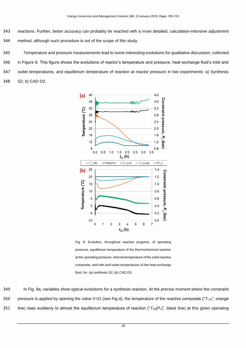
Temperature and pressure measurements lead to some interesting evolutions for qualitative discussion, collected 345
in Figure 8. This figure shows the evolutions of reactor’s temperature and pressure, heat exchange fluid’s inlet and 346
outlet temperatures, and equilibrium temperature of reaction at reactor pressure in two experiments: a) Synthesis 347
S2; b) CAD D3. 348
Fig. 8: Evolution, throughout reaction progress, of operating
pressure, equilibrium temperature of the thermochemical reaction
at the operating pressure, internal temperature of the solid reactive
composite, and inlet and outlet temperatures of the heat exchange
fluid, for: (a) synthesis S2; (b) CAD D3.
In Fig. 8a, variables show typical evolutions for a synthesis reaction. At the precise moment where the constraint 349
pressure is applied by opening the valve V-01 (see Fig.4), the temperature of the reactive composite (“Tr,02”, orange 350
line) rises suddenly to almost the equilibrium temperature of reaction (“Teq(Pc)”, black line) at this given operating 351
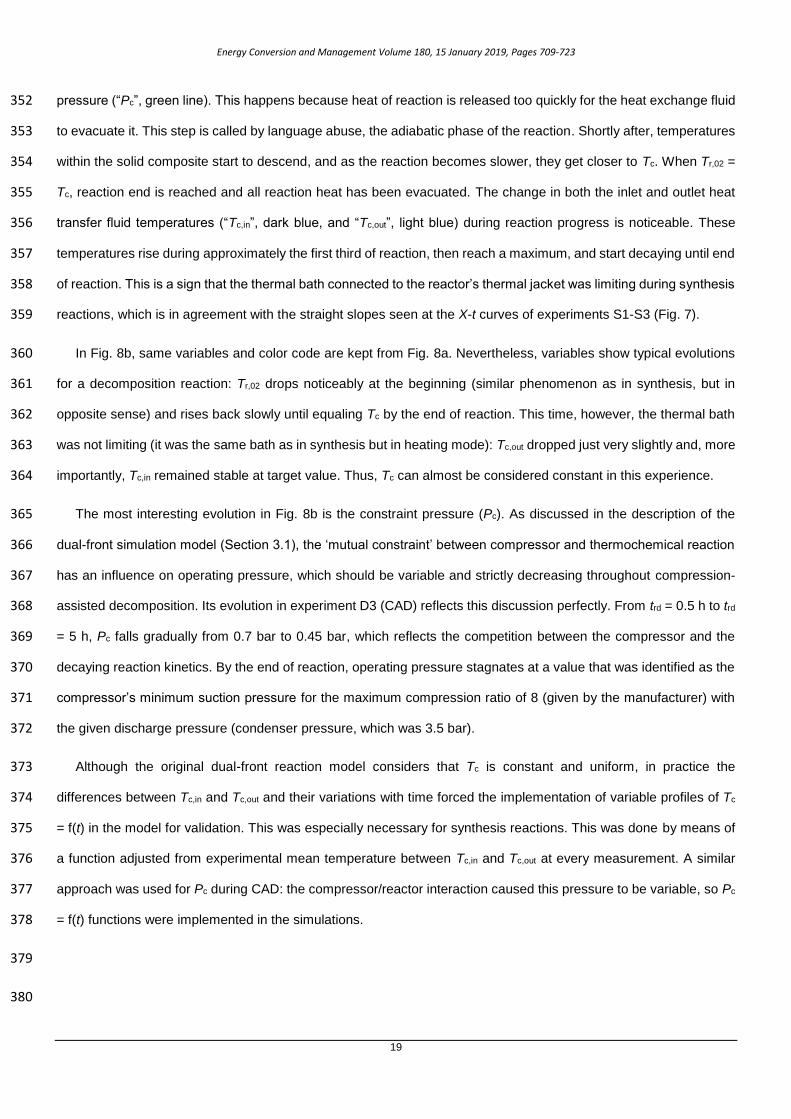
Energy Conversion and Management Volume 180, 15 January 2019, Pages 709-723
19
pressure (“Pc”, green line). This happens because heat of reaction is released too quickly for the heat exchange fluid 352
to evacuate it. This step is called by language abuse, the adiabatic phase of the reaction. Shortly after, temperatures 353
within the solid composite start to descend, and as the reaction becomes slower, they get closer to Tc. When Tr,02 = 354
Tc, reaction end is reached and all reaction heat has been evacuated. The change in both the inlet and outlet heat 355
transfer fluid temperatures (“Tc,in”, dark blue, and “Tc,out”, light blue) during reaction progress is noticeable. These 356
temperatures rise during approximately the first third of reaction, then reach a maximum, and start decaying until end 357
of reaction. This is a sign that the thermal bath connected to the reactor’s thermal jacket was limiting during synthesis 358
reactions, which is in agreement with the straight slopes seen at the X-t curves of experiments S1-S3 (Fig. 7). 359
In Fig. 8b, same variables and color code are kept from Fig. 8a. Nevertheless, variables show typical evolutions 360
for a decomposition reaction: Tr,02 drops noticeably at the beginning (similar phenomenon as in synthesis, but in 361
opposite sense) and rises back slowly until equaling Tc by the end of reaction. This time, however, the thermal bath 362
was not limiting (it was the same bath as in synthesis but in heating mode): Tc,out dropped just very slightly and, more 363
importantly, Tc,in remained stable at target value. Thus, Tc can almost be considered constant in this experience. 364
The most interesting evolution in Fig. 8b is the constraint pressure (Pc). As discussed in the description of the 365
dual-front simulation model (Section 3.1), the ‘mutual constraint’ between compressor and thermochemical reaction 366
has an influence on operating pressure, which should be variable and strictly decreasing throughout compression-367
assisted decomposition. Its evolution in experiment D3 (CAD) reflects this discussion perfectly. From trd = 0.5 h to trd 368
= 5 h, Pc falls gradually from 0.7 bar to 0.45 bar, which reflects the competition between the compressor and the 369
decaying reaction kinetics. By the end of reaction, operating pressure stagnates at a value that was identified as the 370
compressor’s minimum suction pressure for the maximum compression ratio of 8 (given by the manufacturer) with 371
the given discharge pressure (condenser pressure, which was 3.5 bar). 372
Although the original dual-front reaction model considers that Tc is constant and uniform, in practice the 373
differences between Tc,in and Tc,out and their variations with time forced the implementation of variable profiles of Tc 374
= f(t) in the model for validation. This was especially necessary for synthesis reactions. This was done by means of 375
a function adjusted from experimental mean temperature between Tc,in and Tc,out at every measurement. A similar 376
approach was used for Pc during CAD: the compressor/reactor interaction caused this pressure to be variable, so Pc 377
= f(t) functions were implemented in the simulations. 378
379
380

Energy Conversion and Management Volume 180, 15 January 2019, Pages 709-723
20
5. Applicative study 381
The aim of validating the model is to facilitate process simulations for other applications and demonstrate the 382
interest of this hybrid system on representative case. The configuration chosen for this applicative study consists of 383
the HCTRS producing cold at Tev = -25 ºC from an ambient temperature Tm = 20 ºC (which implies condenser 384
temperature of Tcd = 30 ºC). Considering NH3 as working fluid, this temperature difference between cold production 385
and heat rejection would require a too high compression ratio (Ph/Pl= 7.8) to implement the MVC system with a single 386
stage only one vapor compressor refrigerator. 387
5.1. System configuration 388
The hybrid configuration presented in this case (Fig. 9) is based on a two stages vapor compression refrigerator 389
that uses two compressors in series with an optimized intermediate pressure that maximizes overall COP. The 390
ammonia retired from the thermochemical reactor during decomposition is stored inside the ammonia storage tank 391
for later de-storage during synthesis. This means that, except during periods when only the MVC subsystem 392
operates, the ammonia flow rates �̇�9 and �̇�10 are different. 393
Fig. 9: Flow diagram of the configuration considered for the
case study.

Energy Conversion and Management Volume 180, 15 January 2019, Pages 709-723
21
From the point of view of the TCH reaction, the synthesis is assumed to take place simultaneously with MVC cold 394
production, and therefore it is carried out at Pl. As for the decomposition, it has been explained previously that the 395
operating pressure can be adjusted accordingly to heat source temperature. In this particular configuration, 3 options 396
are identified (Fig. 9): 397
1) TOD at Pc,rd = Ph; 398
2) CAD with single-staged compression at Pc,rd = Pm; 399
3) CAD with bi-staged compression at Pc,rd = Pl. 400
For all results shown in this section (except for some cases of Fig. 14), the TCH decomposition was always 401
assumed as option 2 (single-stage CAD at Pc,rd = Pm), and ammonia gas leaving the reactor was assumed to be at 402
the same temperature as the reaction’s equilibrium one at Pc,rd. 403
Figure 10 shows the process on the ammonia’s h-P diagram. The cycle is carried out with total injection, and the 404
three pressure levels are labelled on the diagram. The three options for decomposition of the TCH reactive are also 405
displayed. The same type of compressor was chosen for both high-pressure and low-pressure regions: GEA Bock 406
Open Type Ammonia Compressor, model F14/1366 NH3 [36]. Functions of isentropic efficiency with respect to Pm 407
were derived for both compressors from data in the technical sheet. 408
The determination of the COP, defined by equation 13, is based on energy and mass balances with some classical 409
hypotheses as: steady-state running, isenthalpic expansion through throttle valves, temperatures of ammonia near 410
to ambient temperature after exchange with it (T4 = T18 = Tamb + 5K ; T10 = Tamb + 2K), separator perfectly insulated, 411
no pressure drops in pipes... 412
𝐶𝑂𝑃 =�̇�𝑒𝑣
�̇�𝐿𝑃+ �̇�𝐻𝑃 (13) 413
For the MVC subsystem alone this coefficient depends only of the specific enthalpies hi where the subscript "i" 414
refers to the point "i" in the figures 9 and 10 (eq. 14): 415
𝐶𝑂𝑃𝑀𝑉𝐶 =�̇�𝐿𝑃 ∙ (ℎ1−ℎ13)
�̇�𝐿𝑃 ∙ (ℎ2−ℎ1)+�̇�𝐻𝑃 ∙(ℎ6−ℎ5)=
ℎ1−ℎ13
(ℎ2−ℎ1)+[(ℎ4−ℎ12) (ℎ5−ℎ11)⁄ ]∙(ℎ6−ℎ5) (14) 416
For the HCTRS this coefficient depends also on mass flows exchanged with the reactor, and this one is different 417
during the synthesis (eq. 15) or decomposition (eq. 16): 418

Energy Conversion and Management Volume 180, 15 January 2019, Pages 709-723
22
𝐶𝑂𝑃𝐻𝑌𝐵,𝑠𝑦𝑛 =[�̇�𝐿𝑃+�̇�𝑟𝑠(𝑡)] ∙ (ℎ1−ℎ13)
�̇�𝐿𝑃 ∙ (ℎ2−ℎ1)+�̇�𝐻𝑃 ∙(ℎ6−ℎ5) (15) 419
𝐶𝑂𝑃𝐻𝑌𝐵,𝑑𝑒𝑐 =�̇�𝐿𝑃∙ (ℎ1−ℎ13)−�̇�𝑟𝑑,17𝑐(𝑡) ∙ (ℎ18−ℎ13)
�̇�𝐿𝑃 ∙ (ℎ2−ℎ1)+�̇�𝐻𝑃 ∙(ℎ6−ℎ5) (16) 420
with the mass flows deduced from mass balance and energy balance on the separator respectively for the 421
synthesis phase (eq. 17) and decomposition one (eq. 18): 422
�̇�𝐻𝑃 ∙ (ℎ11 − ℎ5) + �̇�𝐿𝑃 ∙ (ℎ4 − ℎ12) + �̇�𝑟𝑠(𝑡) ∙ (ℎ11 − ℎ12) = 0 (17) 423
�̇�𝐻𝑃 ∙ (ℎ11 − ℎ5) + �̇�𝐿𝑃 ∙ (ℎ4 − ℎ12) + �̇�𝑟𝑑,17𝑏(𝑡) ∙ (ℎ4 − ℎ11) + �̇�𝑟𝑑,17𝑐(𝑡) ∙ (ℎ12 − ℎ11) = 0 (18) 424
Note that �̇�𝑟𝑑,17𝑏(𝑡) and/or �̇�𝑟𝑑,17𝑐(𝑡) may be null in equations (16) and (18) according to the option retained for 425
the CAD. 426
These functions were implemented in the simulation code [37] of the hybrid system, and the COP = f(Pm) diagram 427
was traced (Fig. 11) for optimization. It was found that Pm = 5 bar optimizes COPMVC. It was assumed that the value 428
of Pm that optimizes COPHYB would be very close to this value, for three reasons. First, the MVC subsystem is 429
operating during most of the time. Second, the ammonia stream of the TCH subsystem during CAD is consequently 430
lower than the stream in MVC. Third, optimal Pm for single-stage CAD must prioritize the high-pressure compressor, 431
same as for MVC alone (Fig. 11). 432
Fig. 10: Hybrid compression-thermochemical deep-freezing cycle
represented on the h-P diagram with the configuration that includes
bi-staged compression at the intermediate pressure that optimizes
global system’s COP.
Fig. 11: Global COP optimization of the bi-staged configuration for the
case study. Evolution of COP of the MVC subsystem and compression
ratio of the low-pressure and high-pressure compressors as a function
of intermediate pressure. Optimal intermediate pressure was found at
5 bar by taking into account isentropic efficiency of the two
compressors.

Energy Conversion and Management Volume 180, 15 January 2019, Pages 709-723
23
5.2. Operation scenario 433
Different scenarios are possible. It could be assumed, for instance, that the compressors are driven off-grid by 434
solar-PV electricity. This approach would result in ammonia storage during the day (because of sun availability) and 435
cold production at night (to cover the demand by TCH synthesis since compressors cannot work). Different 436
hypotheses are also applicable for the driving heat: it could be waste heat, or generated by solar thermal collectors, 437
with interesting consequences on operating modes distribution and performance evaluation. 438
The scenario supposed for this applicative study is a permanent cooling load of 40 kW for food freezing in an 439
industrial chamber. Both compressors of the hybrid system are driven by on-grid electricity, and the CAD reactor 440
decomposition is activated with waste heat from another industrial process (therefore, at zero cost). Given the 441
assumptions of constant demand of cold and unlimited availability of both grid electricity and waste heat for a given 442
reactor design, the only decision factor for switching between operating modes is electricity price. It is assumed that 443
the lowest price takes place during the night, while peak prices occur in late evening. Figure 12 represents in “watch 444
shape” the behavior of the HCTRS in this scenario for one full cycle (24 hours, midnight to midnight). 445
Fig. 12: “Watch-shaped” representation of operating periods of
the hybrid compression-thermochemical freezing system in the
case study. Global cycles of 24 hours (midnight to midnight) are
considered, with a total of four different operating periods
throughout the day.
446

Energy Conversion and Management Volume 180, 15 January 2019, Pages 709-723
24
Three operating modes are identified: 447
1) “MVC + CAD” from 00:00 to 06:00, period of lowest electricity price. The whole demand of cold is satisfied 448
by MVC while ammonia from the TCH subsystem is being stored in the ammonia storage tank (in other 449
words, the TCH is charging by means of the endothermic reaction from eq. 1). 450
2) “MVC-only” when electricity price is average. The hybrid system proceeds just as an MVC cycle, and the 451
ammonia of TCH reaction remains stored. This mode is assumed to take place between 06:00 and 18:00 452
and between 22:00 and 00:00. These two periods are represented with distinct colors to differentiate 453
between “MVC-only” with TCH fully charged or fully discharged. 454
3) “MVC + Synthesis” for the peak demand period of 18:00 – 22:00. A part of the cooling load is satisfied by 455
MVC while the other part is covered by discharging ammonia from the storage tank through TCH 456
synthesis (exothermic reaction from eq. 1), reducing consumption of mechanical power by both 457
compressors, and hence electric consumption. 458
Although each operating period is presented as a block in Fig. 12, their distribution in a more realistic case study 459
may well be scattered throughout the day. For instance, another peak electricity price can occur at morning between 460
06:00 and 08:00. Operation of the HCTRS is still feasible in such cases, because the TCH reaction can be interrupted 461
mid-progress and resumed later, with no penalization on total ammonia production. Nevertheless, as this is a 462
preliminary case study, the simplified approach presented here was considered sufficient. 463
Two reactive salts were considered for this case study: SrCl2 and CaCl2, whose activation temperatures for CAD 464
at Pc,dec are suitable for low-grade waste heat utilization (Fig. 3). The calculation procedure combined the dual front 465
quasi-steady reaction model described in Section 3 with a nodal model based on mass and energy balances for 466
global cycle simulation. The calculation process was done in three steps: 467
1) For the given constraint temperature of Tc = Tm = 20 ºC during synthesis phase, adjust reactive 468
composite’s diameter to complete synthesis phase (cold production) within 4 hours (18:00 – 22:00). In 469
this step, the same �̃�𝐸𝑁𝐺 and 𝑤𝑠𝑎 as with experimental implementation of the BaCl2 are kept. This allows 470
to keep also the same values of 𝜆0(= 𝜆1), 𝑘0 (= 𝑘1) and 𝑈𝑤0 (=𝑈𝑤1) that were adjusted for model validation. 471
2) After adjusting composite’s diameter, adjust Th to complete CAD at Pc equal to Pm or Pl, or to complete 472
TOD at Pc equal to Ph, accordingly to the option chosen for the decomposition within 6 hours (00:00 – 473
06:00). 474

Energy Conversion and Management Volume 180, 15 January 2019, Pages 709-723
25
3) Obtain �̇�𝑁𝐻3= 𝑓(𝑡) for synthesis and CAD or TOD and implement these values in the global simulation 475
to obtain data on cold production and power consumption. 476
We propose a performance indicator defined as the COP ratio between the hybrid system and mechanical 477
vapor compression, with COPMVC and COPHYB themselves defined by equations (14) to (16). 478
The value of this indicator is calculated with two different approaches: for Figs. 13 and 14, it is calculated in terms 479
of power at each time step (and noted �̇� , equation (19)), while for Fig. 15 it is calculated in terms of energy (and 480
noted 𝜓) by integrating throughout the whole period of either synthesis (syn , eq. (20)), decomposition (dec , eq. (21)), 481
or the overall thermochemical cycle (syn-dec , eq. (22)). In these cases, as the cooling energy is the same for each 482
period, the ratio of COP is also equal to the ratio of mechanical energy required by the MVC and HCTRS 483
�̇�# = 𝐶𝑂𝑃𝐻𝑌𝐵,#
𝐶𝑂𝑃𝑀𝑉𝐶= 𝑓(𝑡) {# = 𝑠𝑦𝑛, 𝑑𝑒𝑐} (19) 484
𝜓syn = ∫ 𝐶𝑂𝑃𝐻𝑌𝐵,syn∙𝑑𝑡
22ℎ18ℎ
𝐶𝑂𝑃𝑀𝑉𝐶=
∫ (�̇�LP+�̇�HP)𝑀𝑉𝐶∙𝑑𝑡22ℎ
18ℎ
∫ (�̇�LP+�̇�HP)𝐻𝑌𝐵,𝑠𝑦𝑛∙𝑑𝑡22ℎ
18ℎ
(20) 485
𝜓dec = ∫ 𝐶𝑂𝑃𝐻𝑌𝐵,dec∙𝑑𝑡
6ℎ0ℎ
𝐶𝑂𝑃𝑀𝑉𝐶=
∫ (�̇�LP+�̇�HP)𝑀𝑉𝐶∙𝑑𝑡6ℎ
0ℎ
∫ (�̇�LP+�̇�HP)𝐻𝑌𝐵,𝑠𝑦𝑛∙𝑑𝑡6ℎ
0ℎ
(21) 486
𝜓syn−dec = ∫ (�̇�LP+�̇�HP)𝑀𝑉𝐶∙𝑑𝑡
22ℎ18ℎ +∫ (�̇�LP+�̇�HP)𝑀𝑉𝐶∙𝑑𝑡
6ℎ0ℎ
∫ (�̇�LP+�̇�HP)𝐻𝑌𝐵,𝑠𝑦𝑛∙𝑑𝑡22ℎ
18ℎ +∫ (�̇�LP+�̇�HP)𝐻𝑌𝐵,𝑠𝑦𝑛∙𝑑𝑡6ℎ
0ℎ
(22) 487
Note that �̇�𝑀𝑉𝐶 corresponds to the mechanical power consumption of the compressors if all the cooling load was 488
satisfied by MVC exclusively. 489
On the other hand the part of the cooling effect assumed by the TCH subsystem in the hybrid system can be 490
chosen arbitrary (eq. 23) between the two extreme values 0 and 1: 491
𝜀 = 𝑄𝑒𝑣,𝑇𝐶𝐻,𝑠𝑦𝑛
𝑄𝑒𝑣,𝐻𝑌𝐵,𝑠𝑦𝑛 (23) 492
5.3. Results 493
Figure 13 shows results for one full cycle with a dimensioning of the TCH reactor for ε = 0.5 (i.e. to cover 50 % of 494
the cooling load) in the “MVC + Synthesis” period and with Pc equal to Pm during CAD phase. For more clarity, the x-495
axis includes background color traces to distinguish between operating modes that are identical to those of Figure 496
12. Values on the right y-axis correspond to total cooling power (blue line) and power consumption from low-pressure 497

Energy Conversion and Management Volume 180, 15 January 2019, Pages 709-723
26
compressor (purple continuous line) and high-pressure compressor (purple dashed line). Left y-axis is exclusive for 498
the ratio between COP of the hybrid system and COP if all cooling load was covered by MVC alone. 499
Fig. 13: Evolution of COP ratio calculated in terms of power
(�̇�), cooling power and mechanical power consumption of low-
pressure and high-pressure compressors of the bi-staged
hybrid compression-thermochemical freezing system, for one
full cycle (24 hours) at nominal case (ε = 0.5) and Pc,dec = Pm.
Each operating mode is depicted on the x-axis with its
corresponding color (see Fig. 12).
500
The 06:00 – 18:00 and 22:00 – 24:00 periods can be considered as “regular” periods in this figure: all cooling load 501
is satisfied by MVC alone, and power consumption from both compressor remains steady. These values serve for 502
calculation of the COPMVC that is later used for calculation of �̇�. Obviously, in these periods COPHYB = COPMVC, which 503
means �̇� = 1. As for power consumption, that of the high-pressure compressor is lower than that of the low-pressure 504
compressor despite the fact that the mass flow is higher. This is coherent with the fact that Pm = 5 bar yields lower 505
values of HP than of LP and finally better value of the isentropic efficiency for the high-pressure compressor (see 506
Fig. 11). 507
The 00:00 – 06:00 period corresponds to “MVC + CAD”. The cooling load remains constant at target value and is 508
still satisfied by MVC alone, which explains why power consumption from the low-pressure compressor remains the 509
same as in “MVC-only”. However, power consumption from the high-pressure compressor is higher, in accordance 510
with CAD at Pm. Since decomposition is carried out at intermediate pressure, only the high-pressure compressor has 511
increased power consumption. It shows peak consumption at the beginning and decays gradually until the end, and 512
the final value right before switching to the next mode is very close to power consumption in “regular” operation. This 513

Energy Conversion and Management Volume 180, 15 January 2019, Pages 709-723
27
profile is coherent with �̇�𝑟𝑑,𝑁𝐻3= 𝑓(𝑡) during decomposition, since the reaction is faster at the beginning (see Fig. 514
6). This additional power consumption implies �̇� lower than unity, and this parameter follows the same curve as �̇�𝐻𝑃 515
but in the opposite sense. 516
The 18:00 – 22:00 period shows three noteworthy traits: 1) Cold production is variable during the first hour, with 517
a peak of surplus and a peak of shortage; 2) During this same interval, power consumption from both compressors 518
drops to zero; 3) During this same interval, �̇� tends to infinity. 519
The variations of �̇�𝑒𝑣 are caused by the variations of �̇�𝑟𝑠,𝑁𝐻3= 𝑓(𝑡) in thermochemical synthesis, similarly to CAD. 520
Congelation in an industrial chamber usually implies big quantities of food: therefore, the strategy chosen in this study 521
is to let the TCH subsystem produce surplus cold in early synthesis reaction. This surplus cold is stored by the end 522
product itself in the form of slightly lower temperature. This thermal inertia compensates for the sub-par cold 523
production in the later stage of synthesis. As soon as the deficit in cold production equals surplus production from 524
the previous stage, the compressors start working and the remainder of cooling load is supplied by MVC (please 525
note that at this point the TCH subsystem is still producing cold, as shown by a lower power consumption by the 526
compressors between 19h and 22h). 527
The fact that both �̇�𝐿𝑃 and �̇�𝐻𝑃 drop to zero means that the TCH process is covering all cooling load. The whole 528
ammonia stream leaving the evaporator enters the reactor directly, instead of flowing to the compressors. This is 529
synchronized with the surplus/deficit peaks of production. After, power consumption increases gradually as the 530
synthesis reaction advances, since more and more mass flow rate of ammonia is flowing to the compressors. �̇�𝐿𝑃 531
increases faster than �̇�𝐻𝑃 because it compresses a slightly larger stream of ammonia. By the end of the operating 532
period, both power consumptions are close to MVC values, which indicates that the synthesis is close to finishing 533
and the mass flow rate of ammonia entering the reactor is close to zero. 534
The value of �̇� tending to infinity is a logical consequence of power consumption dropping to zero. COPHYB is 535
defined as the ratio of cold production to power consumption, so the denominator reaches 0. Right when compressors 536
start working again, this parameter �̇� decreases back, but always maintaining itself at a value higher than 1.The 537
authors wish to point out that the definition of COPHYB in these calculations does not include the heat of reaction 538
during decomposition, since it is assumed to be waste heat with no cost. Regardless, this figure shows the potential 539
interest of the hybrid system in reducing total power consumption. 540

Energy Conversion and Management Volume 180, 15 January 2019, Pages 709-723
28
Fig. 14: Effect of constraint pressure and temperature of the heat source
on system’s performance during decomposition phase.
541
Figure 14 shows a sensitivity analysis on the influence of other values of Th or Pc during decomposition reaction. 542
This figure can be regarded as a zoomed view of the first 7 hours of operation of Fig. 13, including nominal case 543
(with the same black line as in Fig. 13) and some alternate cases. Three of these alternate cases involve increasing 544
Th at same Pc (= Pm): as a consequence the decomposition finishes earlier than in nominal case, but the drop in �̇� is 545
bigger because peak power consumption is higher. The fourth alternate case involves TOD (Pc = Ph) instead of CAD 546
(Pc = Pm or Pc = Pl), resulting in a constant �̇�𝑑𝑒𝑐 = 1 because Qrd is assumed no-cost and therefore not taken into 547
account for COPHYB definition. Nevertheless, this case requires higher Th than nominal, which can make finding an 548
appropriate waste heat source more difficult. The fifth and final alternate case involves CAD at Pc equal to Pl instead 549
of Pm: this case requires lower Th than nominal, making it easier to find waste heat sources. The downside is a clearly 550
higher power consumption because both compressors proceed during decomposition, while in CAD at intermediate 551
pressure only the high-pressure compressor proceeds. This figure is interesting for analyzing the potential flexibility 552
of this system in adapting to different operating schedules and heat source availability. Main results of the nominal 553
case are shown in Table 3. Some differences can be seen between the process with SrCl2 or with CaCl2. For instance, 554
CaCl2 shows lower activation temperatures at the same operating pressures. On the other hand, reactor volume is 555
smaller with SrCl2 thanks to its higher energy density. 556
557

Energy Conversion and Management Volume 180, 15 January 2019, Pages 709-723
29
Table 3. Operating conditions and performance
figures of the HCTRS in the applicative study at
nominal case (ε = 0.5 and Pc,rd = Pm)
Parameter \ Salt SrCl2 CaCl2
Δhrº [kJ · kmol-NH3-1] 41432 41013
Δsrº [kJ · kmol-NH3-1 · K-1] 132.9 134.4
Msa [kg/kmol] 158.53 110.98
�̃�𝑬𝑵𝑮 [kg/m3] 100
wsa 0.71
Dec [kWh/m3] 125 101
msalt [kg] 313 384
mENG [kg] 127 156
Vr [m3] 1.28 1.57
Th,min [ºC] with Pc = Ph 112.7 99.8
Th,min [ºC] with Pc = Pm 91.0 78.9
Th,min [ºC] with Pc = Pl 66.3 54.4
Ψsyn 2.056 2.066
Ψdec 0.892 0.892
Qev,MVC [kWh] 80.0
Qev,TCH [kWh] 80.0
WLP,syn [kWh] 17.8 17.7
WHP,syn [kWh] 12.2 12.1
WLP,dec [kWh] 56.3 56.3
WHP,dec [kWh] 47.3 47.3
Qrd [kWh] 158.9 157.4
558
Figure 15 shows an analysis of main performance figures in this case study, for several scenarios between = 0 559
(no TCH subsystem at all) and = 1 (all cooling load is provided by TCH during synthesis period) but always (except 560
for =0) with Pc equal to Pm during the CAD periods. The case = 0.5 corresponds to the nominal case. In this figure 561
any indicator with the “syn” subscript, as well as cold production by MVC and TCH, correspond to integration within 562
the whole duration of the “Synthesis” operating mode (18:00 to 22:00). Indicators with the “dec” subscript are 563
calculated by integration within the whole duration of the “MVC + CAD” operating mode. And finally 𝜓𝑠𝑦𝑛−𝑑𝑒𝑐 564
coefficient is calculated by integration within the overall duration of the thermochemical cycle including the synthesis 565
and decomposition reactions (eq. 20 to 22). In the y-axes, magnitudes shown above the zero point are related to the 566

Energy Conversion and Management Volume 180, 15 January 2019, Pages 709-723
30
system’s useful effect: cold production by MVC and TCH shown as bars (left y-axis), and 𝜓 in synthesis, 567
decomposition and overall thermochemical cycle shown as lines (right y-axis). For more clarity a change in scale for 568
𝜓𝑠𝑦𝑛 is operated for the values of upper to the nominal case (> 0.5). On the other hand, magnitudes shown below 569
the zero point are related to the system’s "inputs": compressors’ power consumption during synthesis and 570
decomposition (with yellow and grey bars, left y-axis), heat of decomposition reaction (red bars, left y-axis), and 571
volume of reactive composite (blue line, right y-axis). 572
At = 0, the whole cooling load (40 kW during 4 hours, i.e. 160 kWh) is satisfied by MVC only, which explains the 573
absence of Qev,TCH and Qrd. Also, both dec and syn equal 1 and Vr equals 0, because there is no TCH subsystem at 574
all. At the other extreme case ( = 1) the demand in peak period is entirely covered by the TCH process, so there is 575
no MVC cold production nor compression power consumption during synthesis and 𝜓𝑠𝑦𝑛 goes to infinity. As 576
increases, the TCH process gains more and more presence in the hybrid system and results reflect this tendency. 577
The cooling load is more covered by the thermochemical reaction and less by MVC, and accordingly, mechanical 578
power consumption during synthesis phases becomes lower and lower (yellow bars in Fig. 15). On the other hand, 579
mechanical power consumption in CAD increases gradually (grey bars in Fig. 15), as there is more and more 580
ammonia vapor from the reaction that has to be compressed, so the dec decreases, but moderately until the value 581
of 0.82 at equal to 1. Finally for the overall thermochemical cycle the gain of the COP by the hybrid system is 582
positive; 𝜓𝑠𝑦𝑛−𝑑𝑒𝑐 evolves between 1 and 1.4 for varying from 0 to 1. This tendency of 𝜓𝑠𝑦𝑛−𝑑𝑒𝑐 in the figure 15 583
corresponds also to the ratio between the total cold energy produced (sum of purple and blue bars, i.e. 160 kWh) 584
and the total required mechanical power (sum of yellow and grey bars). Of course this evolution, although positive, 585
is not very important, but we must not forget that the main objective of this hybrid HCTRS, in this case of application, 586
was to reduce particularly the mechanical power absorbed during the hours of peak for electric consumption (i.e. 587
between 18h and 22h); this goal is largely achieved with 𝜓𝑠𝑦𝑛 values of about 2 up to 15.4 for respective values of 588
0.5 and 0.9. 589
Obviously the higher the value the more the volume of the reactor and the thermal power to be supplied to it 590
during the decomposition phases as well. For example (Fig. 15), at equal to 0.8, the volume of the reactive 591
composite is 2m3 and the heat required in decomposition is 250 kWh at 91 °C, again for a cooling production of 160 592
kWh at -25 °C. 593

Energy Conversion and Management Volume 180, 15 January 2019, Pages 709-723
31
Fig. 15: Effect of target share of cold for the thermochemical subsystem (ε) on several variables. In synthesis
phase: COP ratio (ψsyn and ψsyn/10 for ε 0.5) and total cold produced (in kWh) by both subsystems. In
decomposition phase: COP ratio (ψdec), total consumption (in kWh) of mechanical energy by the two
compressors (low-pressure and high-pressure), and total heat consumption (in kWh) by the thermochemical
reactor (at Th = 91°C). For overall thermochemical cycle: total volume (in m3) of reactive composite and global
COP ratio 𝜓𝑠𝑦𝑛−𝑑𝑒𝑐.
The choice of an optimal then derives from the relative importance attributed to the reduction of the electrical 594
consumption and the corresponding increase of the thermal power required for the decomposition phases. The 595
relative cost of the two energies (electrical and thermal) should be taken into account both for the investment of the 596
hybrid system (globally proportional to ) and for its operation. This is outside the scope of this 1st study. 597
6. Conclusions and perspectives 598
The hybrid compression / thermochemical refrigeration system (HCTRS) presented in this paper is expected to 599
valorize low-grade waste heat thanks to the connection between compressor and thermochemical reaction. This 600
hybrid system has three characteristic operating modes, and each one of them allows cold production by mechanical 601
vapor compression while either storing or de-storing refrigerant simultaneously. One of these modes allows additional 602
cold production with no additional power consumption thanks to the thermochemical synthesis reaction. The second 603
mode allows storing refrigerant with no additional power consumption, by using a heat source below 120 ºC. The 604

Energy Conversion and Management Volume 180, 15 January 2019, Pages 709-723
32
third mode connects the compressor and the thermochemical reactor to drop reactor pressure during the refrigerant 605
storage phase, with the idea of reducing heat source temperature. 606
Our experiences proved this reduction in heat source temperature. Thanks to the compressor-reactor coupling, 607
an experiment with the BaCl2/NH3 reaction was possible with a reactor pressure as low as 0.5 bar (condenser 608
pressure being kept at 3.5 bar because one small compressor alone was used). At this pressure, process activation 609
was possible with a heat source at ambient temperature (20 ºC). Without assisting the decomposition reaction with 610
the compressor, reactor pressure would have been 3.5 bar. With this pressure and respecting the same equilibrium 611
drop, process activation would have required a source heat temperature of 55 ºC, i.e. 35K above. 612
To allow further simulations of this system, a quasi-steady simulation model was validated from experimental 613
data, through adjustment of the thermal conductivity and the permeability of the reactive composite, as well as the 614
global heat transfer coefficient between reactive composite and heat transfer fluid from the reactor’s thermal jacket, 615
respectively at the values 1.4 W·m-1·K-1, 10-14 m2 and 170 W·m-2·K-1. The three values are within the reasonable 616
range, based on literature data on thermochemical systems. After parameter adjustment, the quasi-steady simulation 617
model predicted the X-t curves of reaction accurately enough in synthesis, thermally-only activated decomposition 618
and compression-assisted decomposition. In the particular case of compression-assisted decomposition, which is 619
the most characteristic mode of this system, mass transfer limitations were not negligible, given the low operating 620
pressures. 621
The validated quasi-steady simulation model allowed a first law assessment of system performance in a 622
preliminary and nevertheless realistic case study. The scenario was the HCTRS operating in cycles of 24 hours to 623
produce 40 kW cold at -25 ºC for a food conservation industrial chamber, by running a bi-stage MVC cycle with full 624
injection that implies two compressors in series and with a condenser temperature of 30 ºC. From the point of view 625
of electricity source, the compressors were supposed grid-driven and the HCTRS was storing refrigerant in off-peak 626
electric demand periods for later discharge during peak periods. Results indicated that the hybrid can reach, during 627
ammonia de-storage phase, many times higher COP than a mechanical vapor compression refrigeration cycle, 628
depending on the share of cold production (quantified by the parameter) that is covered by the TCH process. 629
The study also considered an alternate case in which compression-assisted decomposition is carried out at a 630
pressure of 1.5 bar, which implies equilibrium temperatures as low as 20 ºC, 35 ºC and 45 ºC for reactions with BaCl2, 631
CaCl2 and SrCl2, respectively. In the particular case of BaCl2, this bi-staged compression can eventually allow 632
process activation with heat at ambient temperature. Our experience D3 proved this activation at ambient 633
Energy Conversion and Management Volume 180, 15 January 2019, Pages 709-723
33
temperature, although condenser pressure was pretty low (3.5 bar) because the experimental bench had just one 634
compression stage. Thus, an experimental study with two compressors in series is definitely an interesting prospect, 635
now that the single-stage compression-assisted decomposition has been experimentally proven. 636
Another interesting question waiting for an answer is whether or not the HCTRS competes economically with 637
state-of-the-art solutions such as electric batteries or phase change materials. Implementing the thermochemical 638
process to a compression refrigeration cycle is probably more expensive than these two options, but as long as a 639
source of free waste heat can be utilized, it can compensate in the long term. After all, both electricity stored by 640
batteries and cold stored by phase change materials come from a surplus consumption of electricity at some point. 641
The HCTRS proceeds the same way, but as long as source heat is free and operating pressure during decomposition 642
can be adjusted, higher heat source temperatures result in lower power consumption by the compressor, and 643
therefore, potentially much higher COP [28]. Moreover, thermochemical processes should have less inertia than 644
batteries in the discharge phase, since the stored material is liquid refrigerant, and can be preferable to phase change 645
materials if no modifications should be made at the cold delivery unit. In addition, the liquid refrigerant is stored at 646
ambient temperature, with no concerns about thermal isolation, which is an advantage in front of other options such 647
as sensible thermal storage. An appropriate economic assessment may eventually answer the question about 648
competitiveness. 649
As final statement the authors of this paper believe that, although the Compression/Thermochemical System may 650
seem less promising than its ‘twin’, i.e. the Expansion/Thermochemical System (electricity and heat inputs for cold 651
production versus heat input for electricity and cold production), its compression-assisted reduction of activation 652
temperature is a powerful enough tool to find a niche. 653
Acknowledgement 654
The authors are thankful for their financial support to the French “ Investments for the future ” program managed 655
by the National Agency for Research under contract ANR-10-LABX-22-01 (Labex SOLSTICE), the Spanish Ministry 656
of Economy and Competitiveness (MINECO) and FEDER/UE (Project DPI2015-71306-R). 657
References 658
[1] Climate Change 2001. The Scientific Basis. Third Assessment Report. UN Intergovernmental Panel on 659
Climate Change. Cambridge University Press, ISBN 0521 01495 6. n.d. 660
[2] Ademe: Le froid alimentaire commercial. Agence de l’Environnement et de la Maîtrise de l’Énergie. 661

Energy Conversion and Management Volume 180, 15 January 2019, Pages 709-723
34
www.ademe.fr [Last updated: 17/12/2014] n.d. 662
[3] Kim DS, Infante Ferreira CA. Solar refrigeration options - a state-of-the-art review. Int J Refrig 2008;31:3–663
15. doi:10.1016/j.ijrefrig.2007.07.011. 664
[4] Cao S, Hasan A, Sirén K. On-site energy matching indices for buildings with energy conversion, storage 665
and hybrid grid connections. Energy Build 2013;64:423–38. doi:10.1016/j.enbuild.2013.05.030. 666
[5] Fitó J, Mauran S, Stitou D, Mazet N, Coronas A. New solar hybrid absorption / thermochemical refrigeration 667
cycle. ECOS 2015 - 28th Int. Conf. Effic. Cost, Optim. Simul. Environ. Impact Energy Syst., 2015. 668
[6] Zeyghami M, Goswami DY, Stefanakos E. A review of solar thermo-mechanical refrigeration and cooling 669
methods. Renew Sustain Energy Rev 2015;51:1428–45. doi:10.1016/j.rser.2015.07.011. 670
[7] El-Bahloul AAM, Ali AHH, Ookawara S. Performance and Sizing of Solar Driven dc Motor Vapor 671
Compression Refrigerator with Thermal Storage in Hot Arid Remote Areas. Energy Procedia 2015;70:634–672
43. doi:10.1016/j.egypro.2015.02.171. 673
[8] Xu Y, Li M, Luo X, Ma X, Wang Y, Li G, et al. Experimental investigation of solar photovoltaic operated ice 674
thermal storage air-conditioning system. Int J Refrig 2018;86:258–72. doi:10.1016/j.ijrefrig.2017.11.035. 675
[9] Bilgili M. Hourly simulation and performance of solar electric-vapor compression refrigeration system. Sol 676
Energy 2011;85:2720–31. doi:10.1016/j.solener.2011.08.013. 677
[10] Mette B, Kerskes H, Drück H. Concepts of long-term thermochemical energy storage for solar thermal 678
applications – Selected examples. Energy Procedia 2012;30:321–30. doi:10.1016/j.egypro.2012.11.038. 679
[11] Stitou D, Mazet N, Mauran S. Experimental investigation of a solid/gas thermochemical storage process for 680
solar air-conditioning. Energy 2012;41:261–70. doi:10.1016/j.energy.2011.07.029. 681
[12] Mauran S, Lahmidi H, Goetz V. Solar heating and cooling by a thermochemical process. First experiments 682
of a prototype storing 60 kW h by a solid/gas reaction. Sol Energy 2008;82:623–36. 683
doi:10.1016/j.solener.2008.01.002. 684
[13] Michel B, Neveu P, Mazet N. Comparison of closed and open thermochemical processes , for long-term 685
thermal energy storage applications. Energy 2014;72:702–16. doi:10.1016/j.energy.2014.05.097. 686
[14] Le Pierrès N, Stitou D, Mazet N. New deep-freezing process using renewable low-grade heat : From the 687
conceptual design to experimental results. Energy 2007;32:600–8. doi:10.1016/j.energy.2006.07.024. 688

Energy Conversion and Management Volume 180, 15 January 2019, Pages 709-723
35
[15] Neveu P, Castaing-Lasvignottes J. Solid-gas chemical heat pumps: Field of application and performance of 689
the internal heat of reaction recovery process. Heat Recover Syst CHP 1993;13:233–51. 690
[16] Li TX, Wu S, Yan T, Xu JX, Wang RZ. A novel solid-gas thermochemical multilevel sorption thermal battery 691
for cascaded solar thermal energy storage. Appl Energy 2016;161:1–10. 692
doi:10.1016/j.apenergy.2015.09.084. 693
[17] Wu S, Li TX, Yan T, Wang RZ. Experimental investigation on a novel solid-gas thermochemical sorption 694
heat transformer for energy upgrade with a large temperature lift. Energy Convers Manag 2017;148:330–8. 695
doi:10.1016/j.enconman.2017.05.041. 696
[18] Jiang L, Wang L, Wang R, Zhu F, Lu Y, Roskilly AP. Experimental investigation on an innovative resorption 697
system for energy storage and upgrade. Energy Convers Manag 2017;138:651–8. 698
doi:10.1016/j.enconman.2017.02.014. 699
[19] Anyanwu EE. Review of solid adsorption solar refrigeration II:: An overview of the principles and theory. 700
Energy Convers Manag 2004;45:1279–95. doi:10.1016/j.enconman.2003.08.003. 701
[20] Bao HS, Wang RZ, Wang LW. A resorption refrigerator driven by low grade thermal energy. Energy 702
Convers Manag 2011;52:2339–44. doi:10.1016/j.enconman.2010.12.045. 703
[21] Mähr C. Vergessene Erfindungen - Warum fährt die Natronlok nicht mehr? DuMont Literatur und Kunst 704
Verlag; 2003. 705
[22] Jahnke A, Ziegler F, Karow M. Re-evaluation of the Honigmann-process: thermo-chemical heat store for the 706
supply of electricity and refrigeration. Proc Heat … 2009. 707
[23] Jahnke A, Strenge L, Fleßner C, Wolf N, Jungnickel T, Ziegler F. First cycle simulations of the honigmann 708
process with LiBr/H2O and NaOH/H2O as working fluid pairs as a thermochemical energy storage. Int J 709
Low-Carbon Technol 2013;8:55–61. doi:10.1093/ijlct/ctt022. 710
[24] Bao H, Ma Z, Roskilly AP. Integrated chemisorption cycles for ultra-low grade heat recovery and thermo-711
electric energy storage and exploitation. Appl Energy 2016;164:228–36. 712
doi:10.1016/j.apenergy.2015.11.052. 713
[25] Bao H, Ma Z, Roskilly AP. A chemisorption power generation cycle with multi-stage expansion driven by low 714
grade heat. Energy Convers Manag 2017;150:956–65. doi:10.1016/j.enconman.2017.07.032. 715
[26] Lu Y, Bao H, Yuan Y, Wang Y, Wang L, Roskilly AP. Optimisation of a novel resorption cogeneration using 716

Energy Conversion and Management Volume 180, 15 January 2019, Pages 709-723
36
mass and heat recovery. Energy Procedia 2014;61:1103–6. doi:10.1016/j.egypro.2014.11.1032. 717
[27] Lu Y, Wang Y, Bao H, Yuan Y, Wang L, Roskilly AP. Analysis of an optimal resorption cogeneration using 718
mass and heat recovery processes. Appl Energy 2015;160:892–901. doi:10.1016/j.apenergy.2015.01.138. 719
[28] Ferrucci F, Stitou D, Ortega P, Lucas F. Mechanical compressor-driven thermochemical storage for cooling 720
applications in tropical insular regions. Concept and efficiency analysis. Appl Energy 2018;219:240–55. 721
doi:10.1016/j.apenergy.2018.03.049. 722
[29] Vasta S, Palomba V, La Rosa D, Mittelbach W. Adsorption-compression cascade cycles: An experimental 723
study. Energy Convers Manag 2018;156:365–75. doi:10.1016/j.enconman.2017.11.061. 724
[30] Fitó J. Solar-driven hybrid refrigeration systems based on thermochemical processes. Doctoral Thesis. 725
Universitat Rovira i Virgili, Tarragona, Spain, 2017. 726
[31] Touzain P. Thermodynamic values of ammonia-salts reactions for chemical sorption heat pumps. Proc. Int. 727
Sorption Heat Pump Conf., München, Germany: 1999, p. 225–36. 728
[32] Hui-Bo L, Mazet N, Coudevylle O, Mauran S. Comparison of a general model with a simplified approach for 729
the transformation of solid-gas media used in chemical heat transformers. Chem Eng Sci 1997;52:311–27. 730
doi:10.1016/S0009-2509(96)00407-1. 731
[33] Fitó J, Mauran S, Stitou D, Mazet N, Coronas A. Solar-driven hybrid absorption-thermochemical 732
refrigeration systems: Performance estimation. Refrig. Sci. Technol., 2016. doi:10.18462/iir.gl.2016.1063. 733
[34] Lahmidi H, Mauran S, Goetz V. Definition, test and simulation of a thermochemical storage process adapted 734
to solar thermal systems. Sol Energy 2006;80:883–93. doi:10.1016/j.solener.2005.01.014. 735
[35] Mauran S, Prades P HF. Heat and mass transfer in consolidated reacting beds for thermochemical systems. 736
Heat Recover Syst CHP 1993;13:315–9. 737
[36] GEA. GEA Open Type Compressors F: The full range of open type compressors and units. 2015. 738
www.gea.com [Visited on June 2018] n.d. 739
[37] Klein SA, Alvarado F. Engineering Equation Solver, Version 10.346. F-Chart software, Middleton. 2005. 740
741