Embed Size (px)
Citation preview
James Chicken
HydraAutomatic Parallelism
Using LLVM
Computer Science Tripos, Part II
Homerton College
8th June 2014
The Lernaean Hydra (LernaÐa CUdra) was, in Greek mythology, a serpent-like watermonster with many heads. For each head cut off, it grew two more.
This project aims to take serial programs and transform them into parallel ones, runningacross multiple threads or machines. This is similar in spirit to how the Hydra, startinglife as a single-headed beast, gradually ended up with many.
The cover image was painted by 19th-century French artist Gustave Moreau, his depiction of the LernaeanHydra. It is in the public domain.
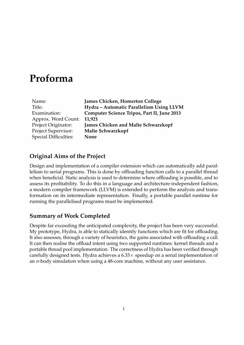
Proforma
Name: James Chicken, Homerton CollegeTitle: Hydra – Automatic Parallelism Using LLVMExamination: Computer Science Tripos, Part II, June 2013Approx. Word Count: 11,921Project Originator: James Chicken and Malte SchwarzkopfProject Supervisor: Malte SchwarzkopfSpecial Difficulties: None
Original Aims of the Project
Design and implementation of a compiler extension which can automatically add paral-lelism to serial programs. This is done by offloading function calls to a parallel threadwhen beneficial. Static analysis is used to determine where offloading is possible, and toassess its profitability. To do this in a language and architecture-independent fashion,a modern compiler framework (LLVM) is extended to perform the analysis and trans-formation on its intermediate representation. Finally, a portable parallel runtime forrunning the parallelised programs must be implemented.
Summary of Work Completed
Despite far exceeding the anticipated complexity, the project has been very successful.My prototype, Hydra, is able to statically identify functions which are fit for offloading.It also assesses, through a variety of heuristics, the gains associated with offloading a call.It can then realise the offload intent using two supported runtimes: kernel threads and aportable thread pool implementation. The correctness of Hydra has been verified throughcarefully designed tests. Hydra achieves a 6.33× speedup on a serial implementation ofan n-body simulation when using a 48-core machine, without any user assistance.
i

Declaration of Originality
I James Chicken of Homerton College, being a candidate for Part II of the ComputerScience Tripos, hereby declare that this dissertation and the work described in it are myown work, unaided except as may be specified below, and that the dissertation does notcontain material that has already been used in any substantial extent for a comparablepurpose.
Signed:
Date: 8th June 2014
ii
Contents
1 Introduction 11.1 Motivations . . . . . . . . . . . . . . . . . . . . . . . . . . . . . . . . . . . . 11.2 Challenges . . . . . . . . . . . . . . . . . . . . . . . . . . . . . . . . . . . . . 21.3 Related Work . . . . . . . . . . . . . . . . . . . . . . . . . . . . . . . . . . . 2
1.3.1 Cilk and OpenMP . . . . . . . . . . . . . . . . . . . . . . . . . . . . 21.3.2 HELIX . . . . . . . . . . . . . . . . . . . . . . . . . . . . . . . . . . . 21.3.3 Vectorisation . . . . . . . . . . . . . . . . . . . . . . . . . . . . . . . 31.3.4 Thread Pools . . . . . . . . . . . . . . . . . . . . . . . . . . . . . . . 3
2 Preparation 52.1 Introduction to Function Offloading . . . . . . . . . . . . . . . . . . . . . . 5
2.1.1 Functions as Tasks . . . . . . . . . . . . . . . . . . . . . . . . . . . . 62.1.2 Limitations . . . . . . . . . . . . . . . . . . . . . . . . . . . . . . . . 8
2.2 Introduction to Threading . . . . . . . . . . . . . . . . . . . . . . . . . . . . 92.2.1 Kernel Threads . . . . . . . . . . . . . . . . . . . . . . . . . . . . . . 102.2.2 Lightweight Threads . . . . . . . . . . . . . . . . . . . . . . . . . . . 10
2.3 Requirements Analysis . . . . . . . . . . . . . . . . . . . . . . . . . . . . . . 132.4 The LLVM Compiler Framework . . . . . . . . . . . . . . . . . . . . . . . . 14
2.4.1 The Need for a Compiler Framework . . . . . . . . . . . . . . . . . 142.4.2 LLVM’s Intermediate Representation . . . . . . . . . . . . . . . . . 142.4.3 LLVM Optimisation Passes . . . . . . . . . . . . . . . . . . . . . . . 182.4.4 Useful Existing LLVM Analysis Passes . . . . . . . . . . . . . . . . 18
2.5 Implementation Approach . . . . . . . . . . . . . . . . . . . . . . . . . . . . 182.6 Choice of Tools . . . . . . . . . . . . . . . . . . . . . . . . . . . . . . . . . . 20
2.6.1 Programming Language — C++ . . . . . . . . . . . . . . . . . . . . 202.6.2 Libraries . . . . . . . . . . . . . . . . . . . . . . . . . . . . . . . . . . 202.6.3 Development Environment . . . . . . . . . . . . . . . . . . . . . . . 20
2.7 Software Engineering Techniques . . . . . . . . . . . . . . . . . . . . . . . . 222.8 Summary . . . . . . . . . . . . . . . . . . . . . . . . . . . . . . . . . . . . . . 22
3 Implementation 233.1 The Fitness Analysis Pass . . . . . . . . . . . . . . . . . . . . . . . . . . . . 23
3.1.1 Fitness Requirements . . . . . . . . . . . . . . . . . . . . . . . . . . . 23
iii
3.1.2 Pointer Arguments . . . . . . . . . . . . . . . . . . . . . . . . . . . . 233.1.3 Global Variables . . . . . . . . . . . . . . . . . . . . . . . . . . . . . 243.1.4 Transitivity of Fitness . . . . . . . . . . . . . . . . . . . . . . . . . . 25
3.2 The Profitability Analysis Pass . . . . . . . . . . . . . . . . . . . . . . . . . 263.2.1 Difficulty of Estimating Profitability . . . . . . . . . . . . . . . . . . 273.2.2 The First Heuristic . . . . . . . . . . . . . . . . . . . . . . . . . . . . 273.2.3 Dealing with Function Calls . . . . . . . . . . . . . . . . . . . . . . . 283.2.4 Dealing with Loops . . . . . . . . . . . . . . . . . . . . . . . . . . . . 293.2.5 Further Work . . . . . . . . . . . . . . . . . . . . . . . . . . . . . . . 31
3.3 The JoinPoints Analysis Pass . . . . . . . . . . . . . . . . . . . . . . . . . . 323.3.1 Detecting Dependencies . . . . . . . . . . . . . . . . . . . . . . . . . 323.3.2 Exactly-Once Joining . . . . . . . . . . . . . . . . . . . . . . . . . . . 333.3.3 At-Least-Once Joining . . . . . . . . . . . . . . . . . . . . . . . . . . 33
3.4 The Decider Analysis Pass . . . . . . . . . . . . . . . . . . . . . . . . . . . . 363.4.1 The Missing Piece . . . . . . . . . . . . . . . . . . . . . . . . . . . . . 363.4.2 Deciding for ‘Exactly-Once’ Runtimes . . . . . . . . . . . . . . . . . 363.4.3 Deciding for ‘At-Least-Once’ Runtimes . . . . . . . . . . . . . . . . 36
3.5 The MakeSpawnable Transformation Pass . . . . . . . . . . . . . . . . . . . 393.5.1 Statement of the Problem . . . . . . . . . . . . . . . . . . . . . . . . 393.5.2 Dealing with Return Values . . . . . . . . . . . . . . . . . . . . . . . 403.5.3 Dealing with User-Defined Types . . . . . . . . . . . . . . . . . . . 40
3.6 The ParalleliseCalls Transformation Pass . . . . . . . . . . . . . . . . . . . 413.6.1 Adding the Runtime API to the Module . . . . . . . . . . . . . . . . 423.6.2 Dealing with the ‘Task’ ID in the Thread Pool . . . . . . . . . . . . . 453.6.3 Switching the Uses of the Return Value . . . . . . . . . . . . . . . . 45
3.7 The Thread Pool . . . . . . . . . . . . . . . . . . . . . . . . . . . . . . . . . . 453.7.1 Initialisation and Layout . . . . . . . . . . . . . . . . . . . . . . . . . 463.7.2 Communicating Tasks to the Worker Threads . . . . . . . . . . . . . 473.7.3 Joining with Worker Threads . . . . . . . . . . . . . . . . . . . . . . 48
3.8 Summary . . . . . . . . . . . . . . . . . . . . . . . . . . . . . . . . . . . . . . 48
4 Evaluation 514.1 Overall Results . . . . . . . . . . . . . . . . . . . . . . . . . . . . . . . . . . 514.2 Unit Tests . . . . . . . . . . . . . . . . . . . . . . . . . . . . . . . . . . . . . . 52
4.2.1 The Fitness Test . . . . . . . . . . . . . . . . . . . . . . . . . . . . . . 524.2.2 The Profitability Test . . . . . . . . . . . . . . . . . . . . . . . . . . . 534.2.3 The JoinPoints Test . . . . . . . . . . . . . . . . . . . . . . . . . . . . 534.2.4 The Decider Test . . . . . . . . . . . . . . . . . . . . . . . . . . . . . 534.2.5 The MakeSpawnable Test . . . . . . . . . . . . . . . . . . . . . . . . 544.2.6 The ParalleliseCalls Test . . . . . . . . . . . . . . . . . . . . . . . . . 54
4.3 Runtime Microbenchmarks . . . . . . . . . . . . . . . . . . . . . . . . . . . 544.4 Performance Testing . . . . . . . . . . . . . . . . . . . . . . . . . . . . . . . 56
4.4.1 High-Confidence Tests . . . . . . . . . . . . . . . . . . . . . . . . . . 57
iv
4.4.2 Scalability Tests . . . . . . . . . . . . . . . . . . . . . . . . . . . . . . 57
5 Conclusions 615.1 Results . . . . . . . . . . . . . . . . . . . . . . . . . . . . . . . . . . . . . . . 615.2 Lessons Learnt . . . . . . . . . . . . . . . . . . . . . . . . . . . . . . . . . . . 625.3 Future Work . . . . . . . . . . . . . . . . . . . . . . . . . . . . . . . . . . . . 62
Bibliography 63
A C++11, the 2011 standard for C++ 65
B Evaluation Code 67B.1 Unit Test Code . . . . . . . . . . . . . . . . . . . . . . . . . . . . . . . . . . . 67
B.1.1 Testing Batch Script – unit-test.sh . . . . . . . . . . . . . . . . . . 67B.1.2 Test Sample . . . . . . . . . . . . . . . . . . . . . . . . . . . . . . . . 69
B.2 Runtime Testing – poolfailuretest.cpp . . . . . . . . . . . . . . . . . . . 69B.3 The n-body simulation – nbody.cpp . . . . . . . . . . . . . . . . . . . . . . 71
C Project Proposal 75C.1 Introduction and Description of the Work . . . . . . . . . . . . . . . . . . . 75C.2 Starting Point . . . . . . . . . . . . . . . . . . . . . . . . . . . . . . . . . . . 76C.3 Substance and Structure of the Project . . . . . . . . . . . . . . . . . . . . . 76
C.3.1 Substance . . . . . . . . . . . . . . . . . . . . . . . . . . . . . . . . . 76C.3.2 Structure . . . . . . . . . . . . . . . . . . . . . . . . . . . . . . . . . . 78C.3.3 Extensions . . . . . . . . . . . . . . . . . . . . . . . . . . . . . . . . . 79
C.4 Success Criterion . . . . . . . . . . . . . . . . . . . . . . . . . . . . . . . . . 80C.5 Timetable and Milestones . . . . . . . . . . . . . . . . . . . . . . . . . . . . 80C.6 Resource Declaration . . . . . . . . . . . . . . . . . . . . . . . . . . . . . . . 82
v

vi
Chapter 1
Introduction
1.1 Motivations
Concurrent and distributed systems have become a ubiquitous part of the moderncomputing landscape. Processor clock speeds have plateaued in recent years, and weare no longer able to write simple serial software and expect it to run twice as fast everycouple of years. The path to faster software is clear: exploit more parallelism.
This is, of course, far from a new revelation: in a modern computing system, we try toextract parallelism from our programs at many levels. Instruction-Level Parallelism (ILP)is the lowest of them, and tends to work rather well. However, there are clear limits toILP, as outlined by Wall [1].
At a higher level, we may extract Thread-Level Parallelism by defining multiple threadsof execution. This is useful if our program has naturally parallel elements – e.g., theindependent physics and AI parts in a game engine. The burden is on programmers tofind and exploit this kind of parallelism, which makes sense as they are best placed toidentify independent, higher level concepts in their programs.
However, writing parallel code is difficult – it may create subtle bugs and securityvulnerabilities which are hard to find and diagnose. Speedups are also not guaranteed,and may be undermined by threading overheads and synchronisation. Finally, thisapproach will not work well on legacy code.
In this project, I aim to use automatic methods to extract a finer-grained level ofparallelism. It is natural for a compiler to reason at a lower level than the high-levelparallelism described above – the compiler understands the dependencies of the codeand the overheads of the threading model. To achieve this, the system I built, Hydra,parallelises function calls so that the caller may resume working before the callee hasfinished.
1
1.2 Challenges
Automatic parallelism comes with many challenges. The first problem one faces is whereto start looking for parallelism. We are generally uninterested in gains of just a fewinstructions due to the synchronisation costs associated with threads – such gains fallunder the domain of ILP. On the other hand, large gains can be very difficult to find andreason about. Can we expect our compilers to understand that components of a game areseparate? As much as we can not expect the compiler to write a program for us, it seemssimilarly unreasonable to expect it to discover these kinds of independent high-levelconcepts in the program.
We need low-level constructs that our compilers can reason about, but which willgive sufficient gains when parallelised. A few come to mind: loops, basic blocks andfunction calls. Loop parallelisation is already a well-explored area, and hence Hydrafocuses on the latter two.
The next challenge is proving independence between these constructs. Independencemakes parallelisation possible, whether it be independence of loop iterations, certainfunction calls or basic blocks. This can be quite challenging in practice, and we mayrespond by restricting the problem or asking the programmer for annotations. Hydratakes the former approach, and requires no programmer input whatsoever.
Finally, there is the choice of threading model. This can have quite serious impli-cations, since Hydra must reject anything for which the gained parallelism does notbalance the added synchronisation. Hydra explores two different threading models, oneof which (§2.2.1) is much more restrictive than the other (§2.2.2).
1.3 Related Work
1.3.1 Cilk and OpenMP
Cilk [2] and OpenMP [3] aim to empower the programmer with concurrency primitivesin C and C++. This is similar to Hydra in that they allow delegation of function calls (see§2.1) and that they provide a runtime system to efficiently implement such primitives.They differ in that Hydra aims to work without any programmer input, while Cilkand OpenMP require the source code to be annotated. In addition, Cilk and OpenMPprimarily target C and C++, whilst Hydra aims to be independent of source language(see §2.4.1).
1.3.2 HELIX
HELIX [4] is a new project which aims to automatically extract loop parallelism fromindependent iterations of a loop. Like Hydra, it works without programmer input andharnesses LLVM to support a variety of languages and targets (see §2.4.1). As discussed
2
in §1.2, Hydra does not focus on loop parallelism, so Hydra and HELIX are orthogonaland complementary.
1.3.3 Vectorisation
Unlike automatic parallelisation, many modern optimising compilers feature automaticvectorisation, for instance, GCC [5] and LLVM through its Polly project [6]. Vectorisation isorthogonal to parallelisation and now considered a separate field, but Hydra is inspiredby the impressive speedups possible, with no programmer input, from vectorisers.
1.3.4 Thread Pools
Hydra provides an implementation of a thread pool (see §3.7), but many of these alreadyexist, for instance libdispatch1 and the Windows Thread Pool.2 These are of highquality, but are not independent of source language and target architecture; hence, aportable thread pool runtimes was implemented for Hydra.
1http://bit.ly/1nwKEkd2http://bit.ly/1jvF9zC
3

4
Chapter 2
Preparation
In this chapter, I will explain all the work that was completed before any code waswritten: the underlying theory (§2.1 and §2.2), requirements identified for a successfulimplementation (§2.3), libraries and tools used (§2.4 and §2.6), details of some earlydesign (§2.5) and principles of engineering established (§2.7).
2.1 Introduction to Function Offloading
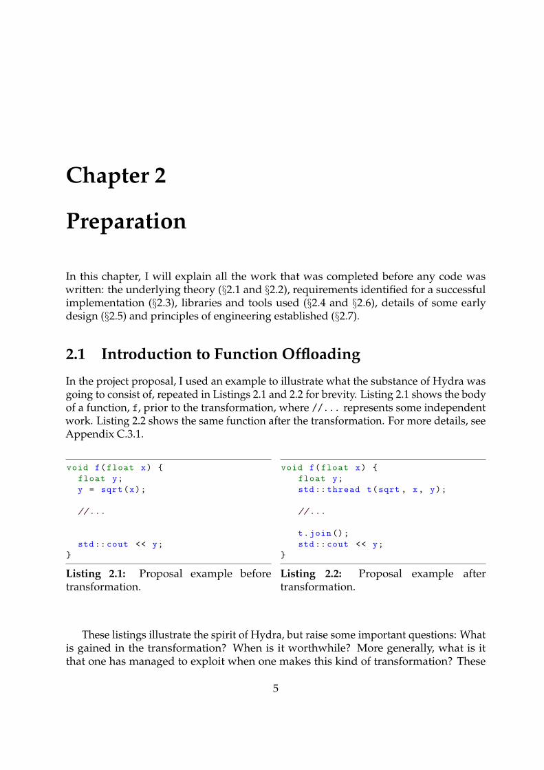
In the project proposal, I used an example to illustrate what the substance of Hydra wasgoing to consist of, repeated in Listings 2.1 and 2.2 for brevity. Listing 2.1 shows the bodyof a function, f, prior to the transformation, where //... represents some independentwork. Listing 2.2 shows the same function after the transformation. For more details, seeAppendix C.3.1.
void f(float x) {
float y;
y = sqrt(x);
//...
std::cout << y;
}
Listing 2.1: Proposal example beforetransformation.
void f(float x) {
float y;
std:: thread t(sqrt , x, y);
//...
t.join();
std::cout << y;
}
Listing 2.2: Proposal example aftertransformation.
These listings illustrate the spirit of Hydra, but raise some important questions: Whatis gained in the transformation? When is it worthwhile? More generally, what is itthat one has managed to exploit when one makes this kind of transformation? These
5
are the questions which I needed to understand before I could begin designing andimplementing Hydra.
2.1.1 Functions as Tasks
Abstractly, we can think of a function call as the delegation of a task. The caller wouldlike some result to be computed, so it delegates the computation of that task to a callee.The callee then computes the required result, and returns it to the caller, which may thenresume its computation.
We can apply this way of thinking to the example above: f needs the square root of x,so it delegates the task of computing it to the sqrt function. sqrt will eventually comeback with the answer, which f then stores in y and continues.
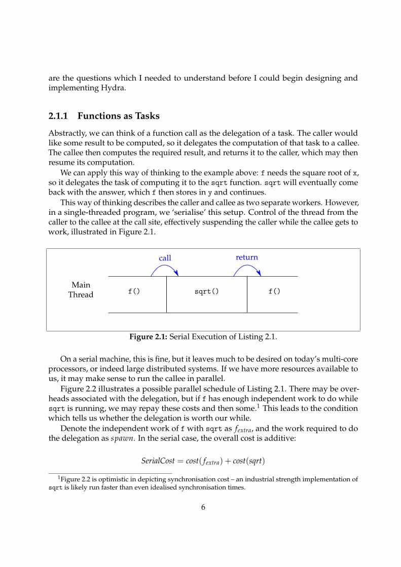
This way of thinking describes the caller and callee as two separate workers. However,in a single-threaded program, we ‘serialise’ this setup. Control of the thread from thecaller to the callee at the call site, effectively suspending the caller while the callee gets towork, illustrated in Figure 2.1.
MainThread f()
call return
f()sqrt()
Figure 2.1: Serial Execution of Listing 2.1.
On a serial machine, this is fine, but it leaves much to be desired on today’s multi-coreprocessors, or indeed large distributed systems. If we have more resources available tous, it may make sense to run the callee in parallel.
Figure 2.2 illustrates a possible parallel schedule of Listing 2.1. There may be over-heads associated with the delegation, but if f has enough independent work to do whilesqrt is running, we may repay these costs and then some.1 This leads to the conditionwhich tells us whether the delegation is worth our while.
Denote the independent work of f with sqrt as fextra, and the work required to dothe delegation as spawn. In the serial case, the overall cost is additive:
SerialCost = cost( fextra) + cost(sqrt)
1Figure 2.2 is optimistic in depicting synchronisation cost – an industrial strength implementation ofsqrt is likely run faster than even idealised synchronisation times.
6
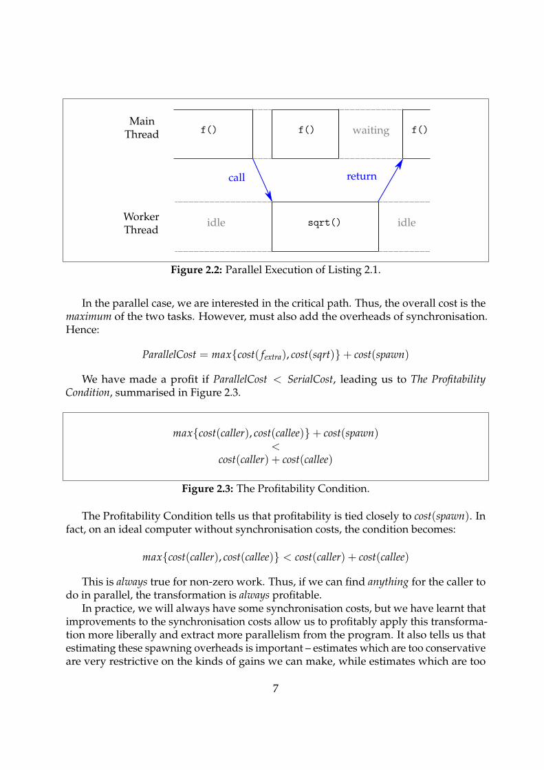
MainThread f() f()
WorkerThread
idle
call return
idlesqrt()
f() waiting
Figure 2.2: Parallel Execution of Listing 2.1.
In the parallel case, we are interested in the critical path. Thus, the overall cost is themaximum of the two tasks. However, must also add the overheads of synchronisation.Hence:
ParallelCost = max{cost( fextra), cost(sqrt)}+ cost(spawn)
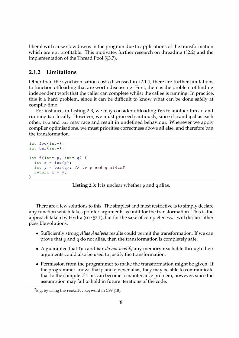
We have made a profit if ParallelCost < SerialCost, leading us to The ProfitabilityCondition, summarised in Figure 2.3.
max{cost(caller), cost(callee)}+ cost(spawn)<
cost(caller) + cost(callee)
Figure 2.3: The Profitability Condition.
The Profitability Condition tells us that profitability is tied closely to cost(spawn). Infact, on an ideal computer without synchronisation costs, the condition becomes:
max{cost(caller), cost(callee)} < cost(caller) + cost(callee)
This is always true for non-zero work. Thus, if we can find anything for the caller todo in parallel, the transformation is always profitable.
In practice, we will always have some synchronisation costs, but we have learnt thatimprovements to the synchronisation costs allow us to profitably apply this transforma-tion more liberally and extract more parallelism from the program. It also tells us thatestimating these spawning overheads is important – estimates which are too conservativeare very restrictive on the kinds of gains we can make, while estimates which are too
7
liberal will cause slowdowns in the program due to applications of the transformationwhich are not profitable. This motivates further research on threading (§2.2) and theimplementation of the Thread Pool (§3.7).
2.1.2 Limitations
Other than the synchronisation costs discussed in §2.1.1, there are further limitationsto function offloading that are worth discussing. First, there is the problem of findingindependent work that the caller can complete whilst the callee is running. In practice,this it a hard problem, since it can be difficult to know what can be done safely atcompile-time.
For instance, in Listing 2.3, we may consider offloading foo to another thread andrunning bar locally. However, we must proceed cautiously, since if p and q alias eachother, foo and bar may race and result in undefined behaviour. Whenever we applycompiler optimisations, we must prioritise correctness above all else, and therefore banthe transformation.
int foo(int*);
int bar(int*);
int f(int* p, int* q) {
int x = foo(p);
int y = bar(q); // do p and q alias?
return x + y;
}
Listing 2.3: It is unclear whether p and q alias.
There are a few solutions to this. The simplest and most restrictive is to simply declareany function which takes pointer arguments as unfit for the transformation. This is theapproach taken by Hydra (see §3.1), but for the sake of completeness, I will discuss otherpossible solutions.
• Sufficiently strong Alias Analysis results could permit the transformation. If we canprove that p and q do not alias, then the transformation is completely safe.
• A guarantee that foo and bar do not modify any memory reachable through theirarguments could also be used to justify the transformation.
• Permission from the programmer to make the transformation might be given. Ifthe programmer knows that p and q never alias, they may be able to communicatethat to the compiler.2 This can become a maintenance problem, however, since theassumption may fail to hold in future iterations of the code.
2E.g. by using the restrict keyword in C99 [10].
8
It is worth noting that, even though Hydra does not consider functions with pointerarguments, primitive alias analysis is still necessary. If, when analysing Listing 2.4, wecannot recognise that the program is using an alias of y, we may decide to join too lateand violate the correctness of the program. This is resolved by SSA form (see §2.4.2).
void f(float x) {
float y;
float *alias = &y; // create an alias for y
y = sqrt(x);
//...
std::cout << *alias; // use that alias
}
Listing 2.4: y is aliased before the call to sqrt.
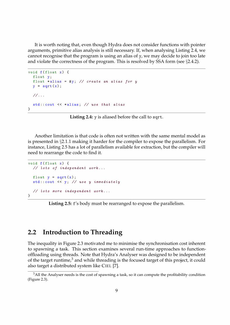
Another limitation is that code is often not written with the same mental model asis presented in §2.1.1 making it harder for the compiler to expose the parallelism. Forinstance, Listing 2.5 has a lot of parallelism available for extraction, but the compiler willneed to rearrange the code to find it.
void f(float x) {
// lots of independent work ...
float y = sqrt(x);
std::cout << y; // use y immediately
// lots more independent work ...
}
Listing 2.5: f’s body must be rearranged to expose the parallelism.
2.2 Introduction to Threading
The inequality in Figure 2.3 motivated me to minimise the synchronisation cost inherentto spawning a task. This section examines several run-time approaches to function-offloading using threads. Note that Hydra’s Analyser was designed to be independentof the target runtime,3 and while threading is the focused target of this project, it couldalso target a distributed system like CIEL [7].
3All the Analyser needs is the cost of spawning a task, so it can compute the profitability condition(Figure 2.3).
9
2.2.1 Kernel Threads
We will begin with a naıve implementation and discuss its limitations. The simplest wayto implement a parallelism run-time system is already illustrated by Listing 2.2 – forevery new task, simply create a brand new kernel thread for it, and join with the threadwhen the result is needed.
This implementation of task parallelism is extremely simple. I used it to facilitatetesting of the compile-time portion before any run-time work was completed, and as abenchmark reference in the evaluation (see §4.4). Unfortunately, this simplicity comes ata price – the cost of creating a new kernel thread is enormous (see §4.3). This ends upheavily restricting the transformation we would like to perform.
There are other problems with this approach. The profitability condition in Figure 2.3masks the problem of having a finite number of cores to actually execute threads. Factor-ing this into the Analyser is tricky – how can it know how many cores are available ata given point in the program? This is best dealt with by the runtime, yet using kernelthreads ignores the problem entirely.
Finally, there is also the problem of creating a very large number of kernel threads onany operating system: thrashing may occur. This is where CPU utilisation is reduced bythe presence of too many kernel threads due to pressure on the scheduler.
2.2.2 Lightweight Threads
The discussion of kernel threads above motivates us to consider alternative approaches.Hydra uses a thread pool of kernel threads initialised at the start of the program, andschedules tasks onto these worker threads via the pool.
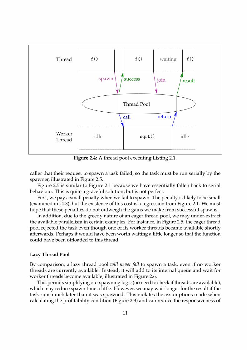
The most interesting question is what happens at spawn-time. I will explore twopossibilities, referred to as eager and lazy thread pools. For both, the behaviour isthe same if there is a worker thread available at spawn time, shown in Figure 2.4.Note the similarity to Figure 2.2, since this is the behaviour we would expect of anytask concurrency implementation when resources are available. Nonetheless, we areimproving on kernel threads by paying the cost of creating threads only once at programinitialisation.
I have been deliberately vague about whether the top thread in Figure 2.4 is the mainthread or a worker thread. In fact, worker threads may ask the thread pool to performtasks on their behalf just like the main thread.
Eager and lazy thread pools differ in their behaviour when all the worker threads areengaged. We shall see that the behaviour of eager thread pools is easier to implement,which is why it was ultimately used (see §3.7).
Eager Thread Pool
At spawn time, an eager thread pool will attempt to service the spawn request immedi-ately. If all the worker threads are currently engaged, the eager thread pool informs the
10
Thread f() f()
spawn join
f() waiting
Thread Pool
success result
WorkerThread
idle
call return
idlesqrt()
Figure 2.4: A thread pool executing Listing 2.1.
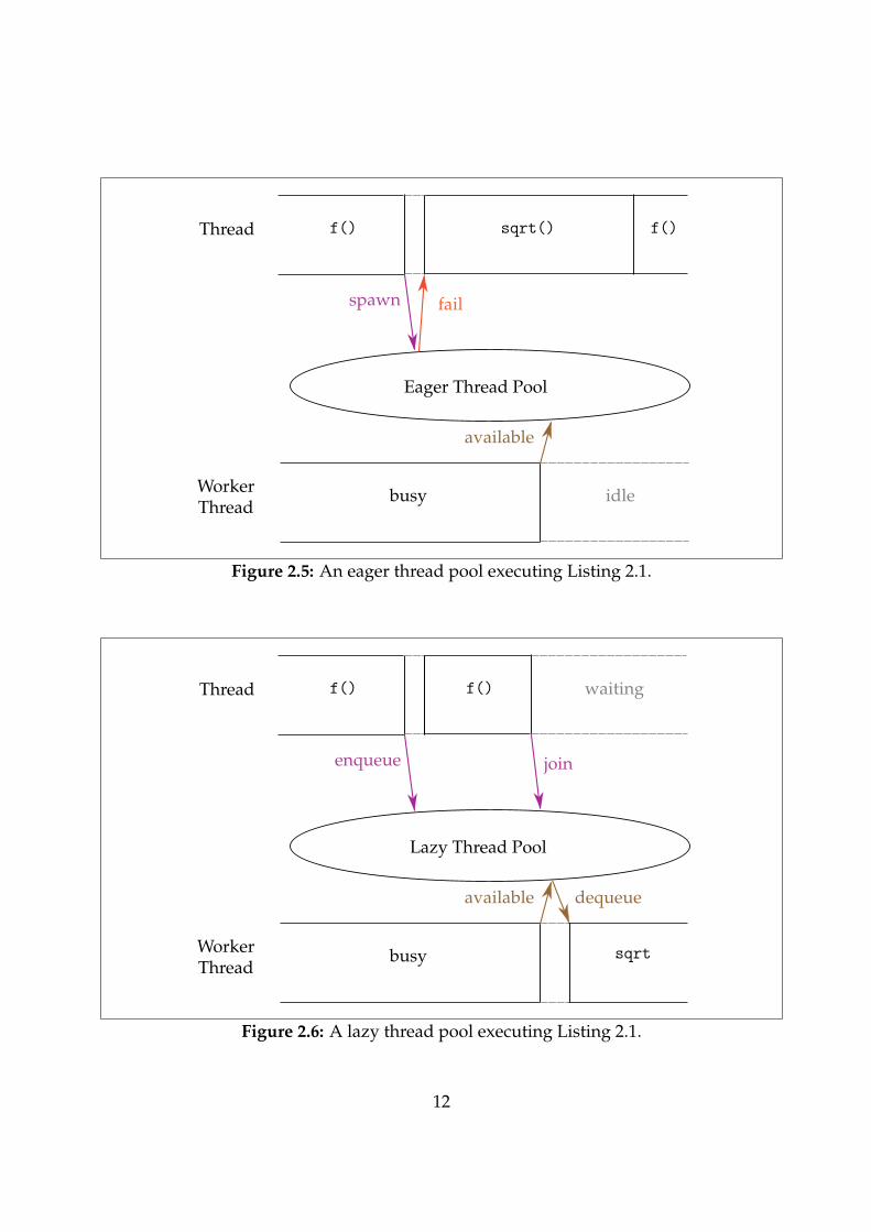
caller that their request to spawn a task failed, so the task must be run serially by thespawner, illustrated in Figure 2.5.
Figure 2.5 is similar to Figure 2.1 because we have essentially fallen back to serialbehaviour. This is quite a graceful solution, but is not perfect.
First, we pay a small penalty when we fail to spawn. The penalty is likely to be small(examined in §4.3), but the existence of this cost is a regression from Figure 2.1. We musthope that these penalties do not outweigh the gains we make from successful spawns.
In addition, due to the greedy nature of an eager thread pool, we may under-extractthe available parallelism in certain examples. For instance, in Figure 2.5, the eager threadpool rejected the task even though one of its worker threads became available shortlyafterwards. Perhaps it would have been worth waiting a little longer so that the functioncould have been offloaded to this thread.
Lazy Thread Pool
By comparison, a lazy thread pool will never fail to spawn a task, even if no workerthreads are currently available. Instead, it will add to its internal queue and wait forworker threads become available, illustrated in Figure 2.6.
This permits simplifying our spawning logic (no need to check if threads are available),which may reduce spawn time a little. However, we may wait longer for the result if thetask runs much later than it was spawned. This violates the assumptions made whencalculating the profitability condition (Figure 2.3) and can reduce the responsiveness of
11
Thread f() f()
spawn
sqrt()
Eager Thread Pool
fail
WorkerThread
idlebusy
available
Figure 2.5: An eager thread pool executing Listing 2.1.
Thread f()
enqueue
Lazy Thread Pool
WorkerThread
busy
available
f() waiting
join
dequeue
sqrt
Figure 2.6: A lazy thread pool executing Listing 2.1.
12
the application, even though throughput may have increased. A lazy pool also carriesmore state than an eager one which may be a concern if memory is tight.
Alternatives
We can overcome the limitations of lazy pools with a work-conserving approach – i.e. byrunning the spawned work if it has not begun at join-time. This allows a small windowfor threads to become available, without running into the case where several threads areall waiting for their tasks to finish (possibly in dead-lock), even though those tasks are justsitting on the queue.
Another alternative is to use a threading model without joins. To achieve this for theprogram in Listing 2.1, we would need to split f into three parts, f before, f during andf after, and communicate a dependency graph to the runtime. Here, f before has nodependencies, f during & sqrt depend on f before, and f after depends on f during
& sqrt. This approach is employed in projects like libdispatch (see §1.3.4).
2.3 Requirements Analysis
Hydra divides naturally into three core elements – the Analyser, the Transformer and theThread Pool. This facilitates modularisation, and allows their requirements to be specifiedseparately.
Consulting the success criterion from the project’s proposal (Appendix C.4), the keyrequirements for my project are as follows:
Analyser — high priorityRequired to determine which functions are fit for spawning and, through variousheuristics and applications of the profitability condition (Figure 2.3), at whichcallsites of those functions offloading is profitable in a supported runtime.
Transformer — medium priorityRequired to do all that is necessary to communicate to a supported runtime thatcertain function calls, which the Analyser deemed appropriate, should be offloaded.
Thread Pool — low priorityRequired to be an implementation of a supported runtime of the Analyser andTransformer which performs function offloading using an Eager Thread Pool design(§2.2.2).
In the requirements above, I used the phrase supported runtime to refer to a runtimesystem, supported by Hydra, capable of performing function offloading (§2.1).4
The priority of each component was important to identify. I decided that the Analyseris the most crucial part of Hydra, and so was given the highest priority. The Transformer
4The two supported runtimes of Hydra are Kernel Threads (§2.2.1) and the Thread Pool (§3.7).
13
is necessary for performing most of this project’s empirical evaluation (see §4), so camenext. Finally, the Thread Pool was assigned the lowest priority since it is not requiredfor a minimum successful project. Despite this, the Thread Pool was still an importantcomponent, since the project was unlikely to offer performance gains without it.
Dependencies between these elements are small, but worth discussing. The Analyserneeds to know the cost of offloading on all supported runtimes so that it can com-pute the profitability condition, although this can be ‘stubbed out’ for the purposes ofdevelopment. The Thread Pool has very few dependencies on the rest of the project.
The Transformer, however, needed interfaces to the Analyser and all supportedruntimes to be specified before its development could begin. Thus, specifying theseinterfaces was an important first step in Hydra’s implementation.
2.4 The LLVM Compiler Framework
The LLVM modular compiler framework [8] is core to Hydra. I spent the vast majority ofmy research time learning about it and will discuss what I learnt here.
2.4.1 The Need for a Compiler Framework
When I had the idea for Hydra, I wanted to focus on the more general problem ofautomatic parallelism, without concentrating on issues specific to certain languages ortargets. However, I did not want to create a disproportionate amount of additional work,since my vision was for Hydra to be about automatic parallelism, rather than a languageand target-independent compilation.
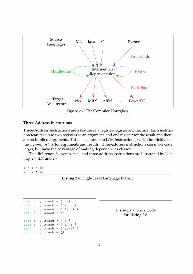
These ideas of language- and target-independence are well known in the field of com-piler construction. Rather than writing MN compilers to compile M source languagesto N target architectures, an Intermediate Representation (IR) is established, illustrated inFigure 2.7. Armed with an IR, adding a new language involves writing one Front-End,and adding a new target involves writing one Back-End.
The use of an IR gives us a natural way to write source-target independent optimisa-tions, by using an IR-to-IR Optimiser, which is sometimes referred to as the “Middle-End”of the compiler. This is where Hydra lives.
2.4.2 LLVM’s Intermediate Representation
LLVM is centred around a well-specified intermediate representation, the LLVM IR.Unlike other IRs like Java Bytecode, LLVM IR is specifically designed for compileroptimisations, rather than interpretation. As such, LLVM IR features Three-AddressInstructions and has Static Single Assignment Form. It is also organised into Basic Blocks.All of these simplify the task of finding join points (see §3.3).
14
SourceLanguages
ML Java C Python...
IntermediateRepresentation
Front-Ends
TargetArchitectures
x86 MIPS ARM PowerPC...
Back-Ends
Middle-End Hydra
Figure 2.7: The Compiler Hourglass.
Three-Address Instructions
Three-Address Instructions are a feature of a register-register architecture. Each instruc-tion features up to two registers as an argument, and one register for the result and thereare no implied arguments. This is in contrast to JVM instructions, which implicitly usethe argument-stack for arguments and results. Three-address instructions can make codelarger, but have the advantage of making dependencies clearer.
The differences between stack and three-address instructions are illustrated by List-ings 2.6, 2.7, and 2.8.
a = b - c;
b = c - d;
Listing 2.6: High-Level Language Extract.
push b ; stack = { b }
push c ; stack = { b, c }
sub ; stack = { (b-c) }
pop a ; stack = {}
push c ; stack = { c }
push d ; stack = { c, d }
sub ; stack = { (c-d) }
pop b ; stack = {}
Listing 2.7: Stack Codefor Listing 2.6.
15
load R1 b ; R1 := b
load R2 c ; R2 := c
sub R3 R1 R2 ; R3 := R1-R2
store a R3 ; a := R3
load R4 c ; R4 := c
load R5 d ; R5 := d
sub R6 R4 R5 ; R6 := R4 -R5
store b R6 ; b := R6
Listing 2.8: Three-Address Codefor Listing 2.6.
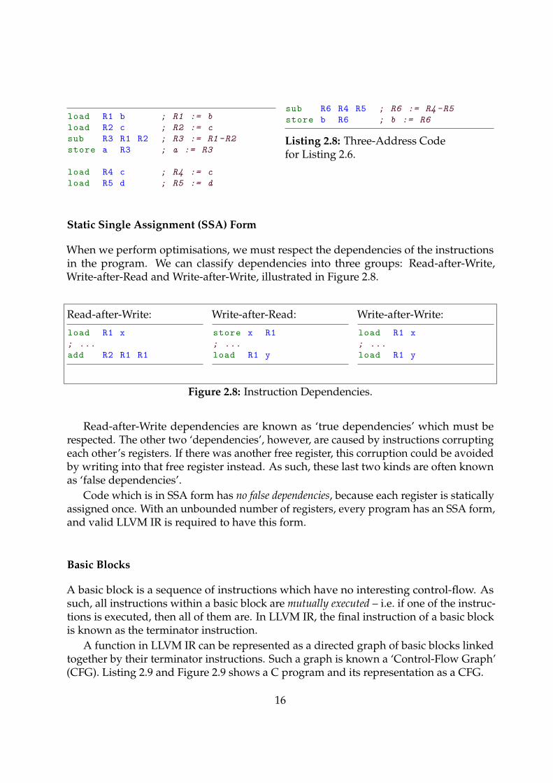
Static Single Assignment (SSA) Form
When we perform optimisations, we must respect the dependencies of the instructionsin the program. We can classify dependencies into three groups: Read-after-Write,Write-after-Read and Write-after-Write, illustrated in Figure 2.8.
Read-after-Write:
load R1 x
; ...
add R2 R1 R1
Write-after-Read:
store x R1
; ...
load R1 y
Write-after-Write:
load R1 x
; ...
load R1 y
Figure 2.8: Instruction Dependencies.
Read-after-Write dependencies are known as ‘true dependencies’ which must berespected. The other two ‘dependencies’, however, are caused by instructions corruptingeach other’s registers. If there was another free register, this corruption could be avoidedby writing into that free register instead. As such, these last two kinds are often knownas ‘false dependencies’.
Code which is in SSA form has no false dependencies, because each register is staticallyassigned once. With an unbounded number of registers, every program has an SSA form,and valid LLVM IR is required to have this form.
Basic Blocks
A basic block is a sequence of instructions which have no interesting control-flow. Assuch, all instructions within a basic block are mutually executed – i.e. if one of the instruc-tions is executed, then all of them are. In LLVM IR, the final instruction of a basic blockis known as the terminator instruction.
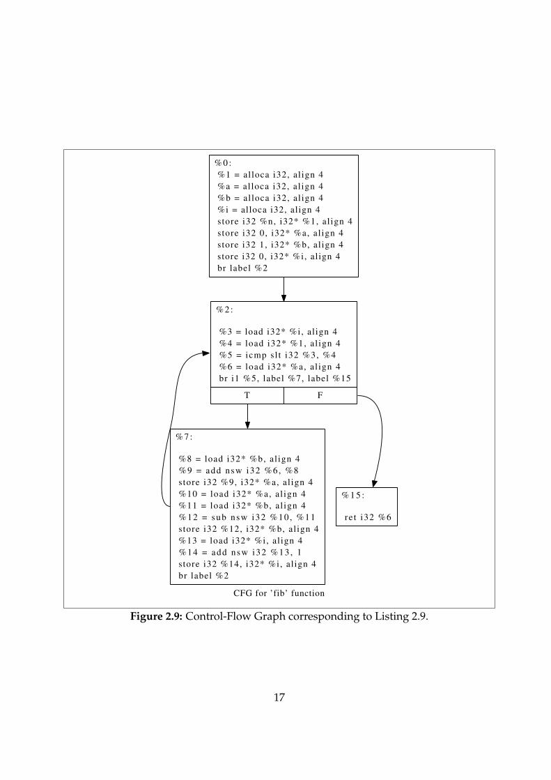
A function in LLVM IR can be represented as a directed graph of basic blocks linkedtogether by their terminator instructions. Such a graph is known a ‘Control-Flow Graph’(CFG). Listing 2.9 and Figure 2.9 shows a C program and its representation as a CFG.
16
CFG for ’fib’ function
% 0 :
%1 = alloca i32, align 4
%a = alloca i32, al ign 4
%b = alloca i32, align 4
%i = alloca i32, align 4
store i32 %n, i32* %1, al ign 4
store i32 0, i32* %a, al ign 4
store i32 1, i32* %b, align 4
store i32 0, i32* %i, align 4
br label %2
% 2 :
%3 = load i32* %i, align 4
%4 = load i32* %1, al ign 4
%5 = icmp sl t i32 %3, %4
%6 = load i32* %a, al ign 4
br i1 %5, label %7, label %15
T F
% 7 :
%8 = load i32* %b, al ign 4
%9 = add nsw i32 %6, %8
store i32 %9, i32* %a, al ign 4
%10 = load i32* %a, al ign 4
%11 = load i32* %b, al ign 4
%12 = sub nsw i32 %10 , %11
store i32 %12, i32* %b, al ign 4
%13 = load i32* %i, al ign 4
%14 = add nsw i32 %13 , 1
store i32 %14, i32* %i, align 4
br label %2
% 1 5 :
re t i32 %6
Figure 2.9: Control-Flow Graph corresponding to Listing 2.9.
17
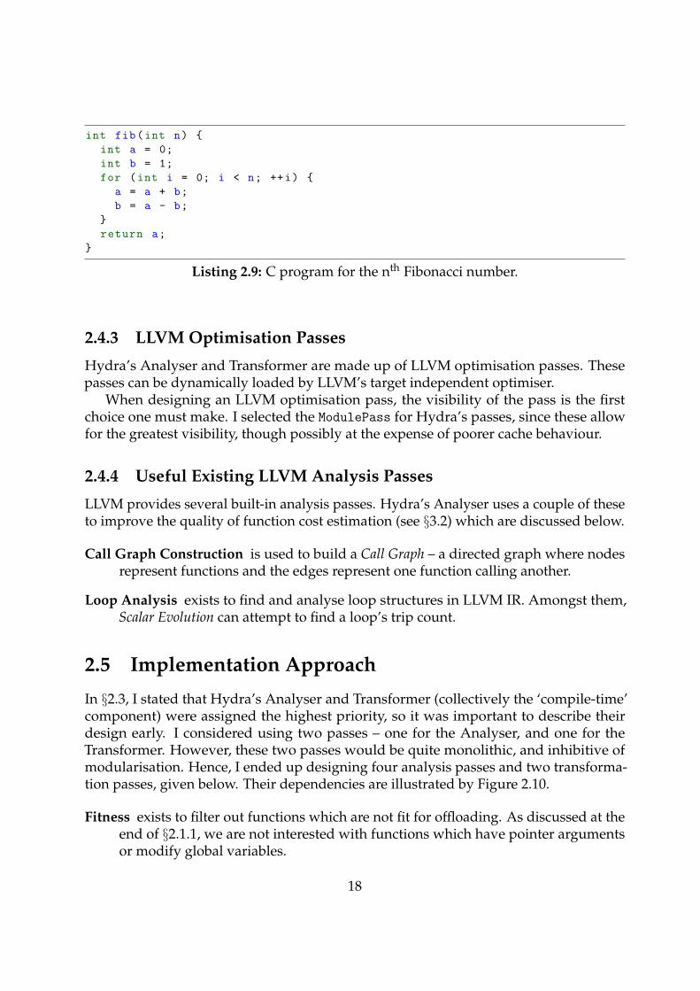
int fib(int n) {
int a = 0;
int b = 1;
for (int i = 0; i < n; ++i) {
a = a + b;
b = a - b;
}
return a;
}
Listing 2.9: C program for the nth Fibonacci number.
2.4.3 LLVM Optimisation Passes
Hydra’s Analyser and Transformer are made up of LLVM optimisation passes. Thesepasses can be dynamically loaded by LLVM’s target independent optimiser.
When designing an LLVM optimisation pass, the visibility of the pass is the firstchoice one must make. I selected the ModulePass for Hydra’s passes, since these allowfor the greatest visibility, though possibly at the expense of poorer cache behaviour.
2.4.4 Useful Existing LLVM Analysis Passes
LLVM provides several built-in analysis passes. Hydra’s Analyser uses a couple of theseto improve the quality of function cost estimation (see §3.2) which are discussed below.
Call Graph Construction is used to build a Call Graph – a directed graph where nodesrepresent functions and the edges represent one function calling another.
Loop Analysis exists to find and analyse loop structures in LLVM IR. Amongst them,Scalar Evolution can attempt to find a loop’s trip count.
2.5 Implementation Approach
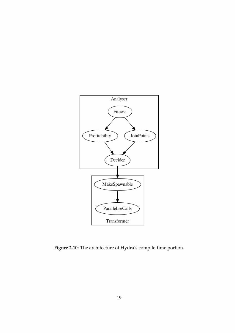
In §2.3, I stated that Hydra’s Analyser and Transformer (collectively the ‘compile-time’component) were assigned the highest priority, so it was important to describe theirdesign early. I considered using two passes – one for the Analyser, and one for theTransformer. However, these two passes would be quite monolithic, and inhibitive ofmodularisation. Hence, I ended up designing four analysis passes and two transforma-tion passes, given below. Their dependencies are illustrated by Figure 2.10.
Fitness exists to filter out functions which are not fit for offloading. As discussed at theend of §2.1.1, we are not interested with functions which have pointer argumentsor modify global variables.
18
Analyser
Transformer
Fitness
Profitability JoinPoints
Decider
MakeSpawnable
ParalleliseCalls
Figure 2.10: The architecture of Hydra’s compile-time portion.
19
Profitability tries to estimate the cost of calling each function. This essentially calculatesthe cost(callee) from the Profitability Condition (Figure 2.3).
JoinPoints exists to find where to join with the callee would be. Pushing this back as faras possible will yield better results, but the correctness of the program cannot bealtered by violating instruction dependencies.
The Decider gets the final say on whether we shall parallelise. It can see all the datagathered from previous analysis passes. The decision is made by applying theProfitability Condition (Figure 2.3), but to do this, it must calculate cost(caller).
MakeSpawnable synthesises a ‘spawnable’ version of each function which the Deciderchose to spawn. This helps Hydra deal with return values and user defined types.
ParalleliseCalls does the ‘dirty work’ of the Transformer, by replacing each call whichthe Decider chose to parallelise with spawn intrinsics for the target runtime, andswitching all the old users of the return value with the new return value.
2.6 Choice of Tools
2.6.1 Programming Language — C++
C++ is the most natural implementation language for Hydra. The primary reason isthat the interface to LLVM is a C++ interface. In addition, I was already proficient inC++ when proposing the project. I decided to use C++11 for Hydra, as discussed inAppendix A.
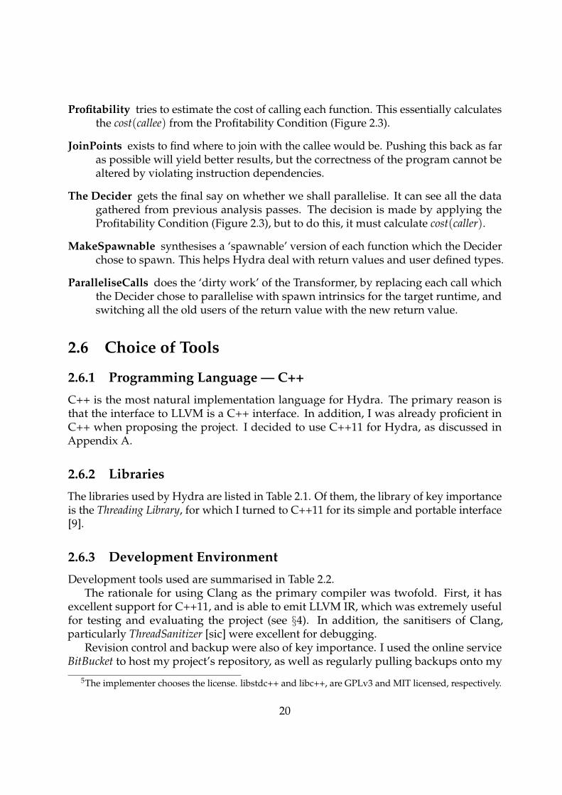
2.6.2 Libraries
The libraries used by Hydra are listed in Table 2.1. Of them, the library of key importanceis the Threading Library, for which I turned to C++11 for its simple and portable interface[9].
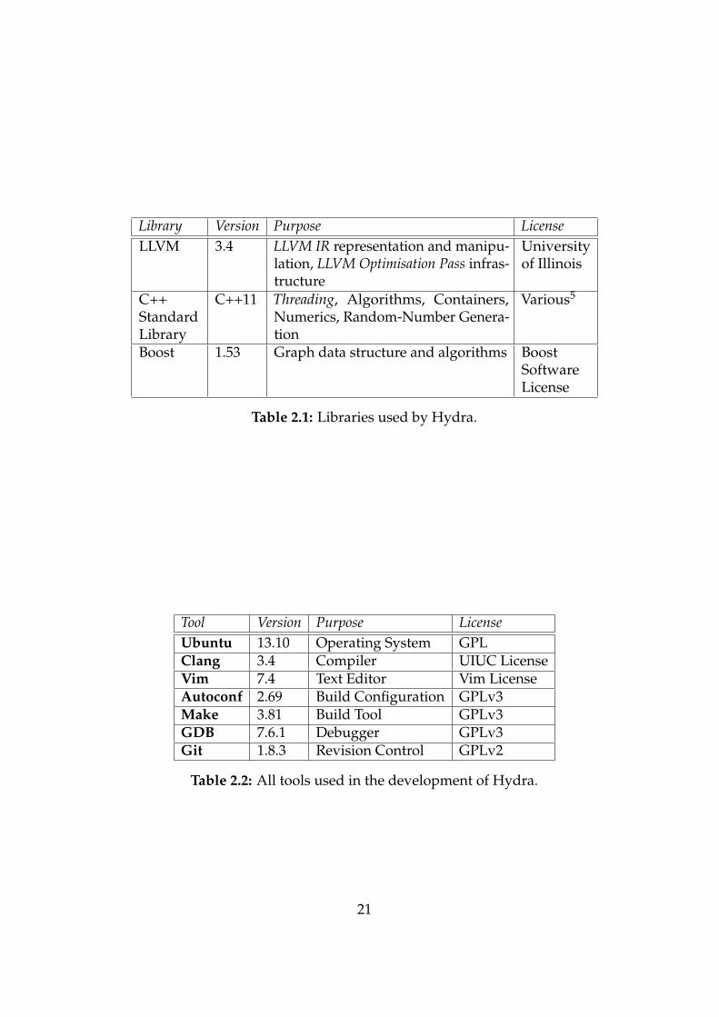
2.6.3 Development Environment
Development tools used are summarised in Table 2.2.The rationale for using Clang as the primary compiler was twofold. First, it has
excellent support for C++11, and is able to emit LLVM IR, which was extremely usefulfor testing and evaluating the project (see §4). In addition, the sanitisers of Clang,particularly ThreadSanitizer [sic] were excellent for debugging.
Revision control and backup were also of key importance. I used the online serviceBitBucket to host my project’s repository, as well as regularly pulling backups onto my
5The implementer chooses the license. libstdc++ and libc++, are GPLv3 and MIT licensed, respectively.
20
Library Version Purpose LicenseLLVM 3.4 LLVM IR representation and manipu-
lation, LLVM Optimisation Pass infras-tructure
Universityof Illinois
C++StandardLibrary
C++11 Threading, Algorithms, Containers,Numerics, Random-Number Genera-tion
Various5
Boost 1.53 Graph data structure and algorithms BoostSoftwareLicense
Table 2.1: Libraries used by Hydra.
Tool Version Purpose LicenseUbuntu 13.10 Operating System GPLClang 3.4 Compiler UIUC LicenseVim 7.4 Text Editor Vim LicenseAutoconf 2.69 Build Configuration GPLv3Make 3.81 Build Tool GPLv3GDB 7.6.1 Debugger GPLv3Git 1.8.3 Revision Control GPLv2
Table 2.2: All tools used in the development of Hydra.
21
two development machines. I also used this repository with my LATEX source files for theproposal and dissertation.
2.7 Software Engineering Techniques
I used an Iterative Development Model when engineering the project. Proper modulari-sation and encapsulation of certain parts of the software was vital to allow each of thecomponents to be developed in isolation, and I used C++ features of classes, namespaces,access control and immutability to aid in this. In addition, proper interfaces were speci-fied using class declarations, and header files were carefully designed to be self-containedand include only the files needed.
In addition, I maintained a level of discipline when developing the software and ad-hered to good practices, such as treating compiler warnings as errors, adding commentswhere the code is subtle or unclear, programming in a structured and defensive style,and using assertions where appropriate.
2.8 Summary
In this chapter, I have discussed the work completed before the implementation began. Idiscussed the surrounding theory in detail, and talked about the design goals of Hydra,as well as the tools and techniques used – in particular, how LLVM is fundamental toHydra’s success.
The next chapter will give details on how the goals and designs laid out here wereachieved.
22
Chapter 3
Implementation
This chapter explains how the designs from the previous chapter were realised. Hydra isdiscussed as seven pieces: fitness (§3.1) and profitability (§3.2) of functions, finding joinpoints (§3.3), the final decision (§3.4), making functions spawnable (§3.5), parallelisingcalls (§3.6) and the Thread Pool runtime (§3.7).
3.1 The Fitness Analysis Pass
The first thing done in the Analyser is to check which functions of the program canpossibly be offloaded. Doing this first makes a lot of sense, since we need not waste timeperforming further analysis on functions which cannot be offloaded.
3.1.1 Fitness Requirements
To be fit, a function may not have pointer arguments or access global variables. As such,these functions are ‘pure’ in the sense that they depend only on their arguments andnever on global state.
These restrictions make the project more tractable than it would be otherwise, asdiscussed in §2.1.2. Any relaxations to the above must be accompanied by alias analysis,which is a hard problem. The potential gains from lifting such restrictions dependsstrongly on the quality of the alias analysis.
3.1.2 Pointer Arguments
To discover whether a function uses pointer arguments, Hydra looks at the function’ssignature. The implementation, given in Listing 3.1, checks if any of the function’sarguments is of pointer type. Hydra identifies all functions with pointer arguments byrunning the checker on each one.
23
bool hasPointerArgs(const llvm:: Function &F) {
return std:: any_of(F.arg_begin (), F.arg_end (),
[]( const llvm:: Argument &arg) {
return arg.getType ()->isPointerTy ();
});
}
Listing 3.1: The pointer arguments checker used in Hydra.
3.1.3 Global Variables
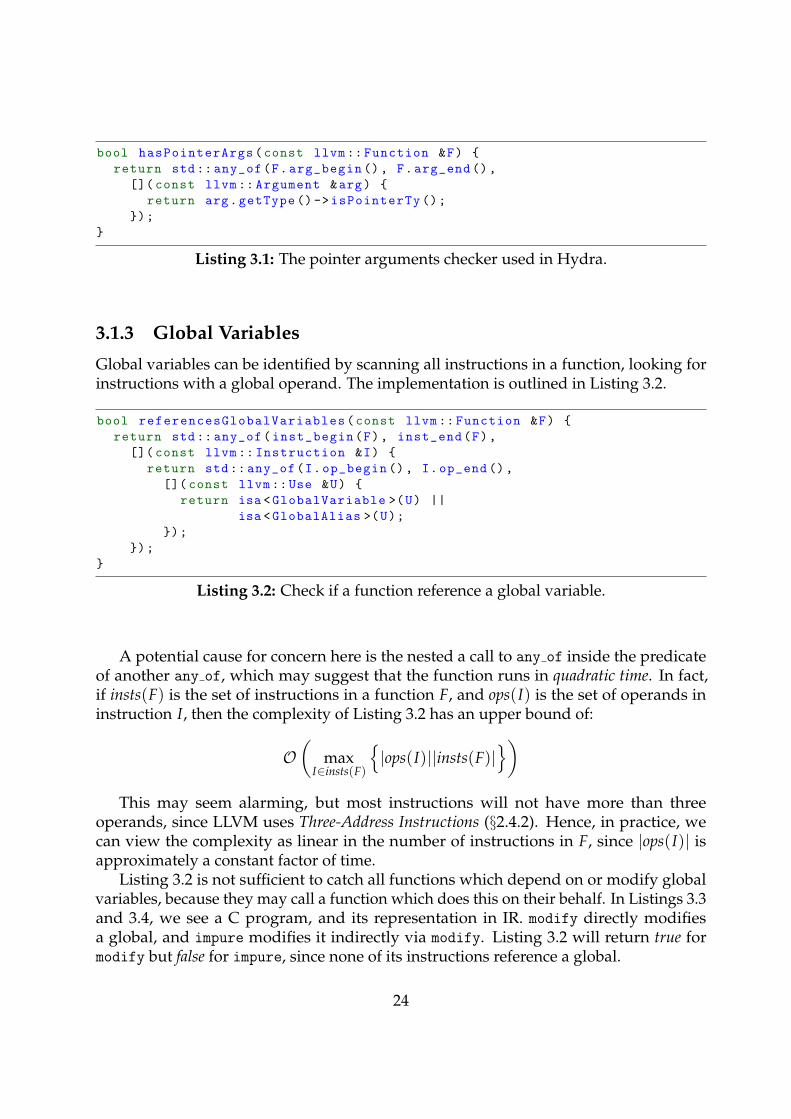
Global variables can be identified by scanning all instructions in a function, looking forinstructions with a global operand. The implementation is outlined in Listing 3.2.
bool referencesGlobalVariables(const llvm:: Function &F) {
return std:: any_of(inst_begin(F), inst_end(F),
[]( const llvm:: Instruction &I) {
return std:: any_of(I.op_begin (), I.op_end (),
[]( const llvm::Use &U) {
return isa <GlobalVariable >(U) ||
isa <GlobalAlias >(U);
});
});
}
Listing 3.2: Check if a function reference a global variable.
A potential cause for concern here is the nested a call to any of inside the predicateof another any of, which may suggest that the function runs in quadratic time. In fact,if insts(F) is the set of instructions in a function F, and ops(I) is the set of operands ininstruction I, then the complexity of Listing 3.2 has an upper bound of:
O(
maxI∈insts(F)
{|ops(I)||insts(F)|
})This may seem alarming, but most instructions will not have more than three
operands, since LLVM uses Three-Address Instructions (§2.4.2). Hence, in practice, wecan view the complexity as linear in the number of instructions in F, since |ops(I)| isapproximately a constant factor of time.
Listing 3.2 is not sufficient to catch all functions which depend on or modify globalvariables, because they may call a function which does this on their behalf. In Listings 3.3and 3.4, we see a C program, and its representation in IR. modify directly modifiesa global, and impure modifies it indirectly via modify. Listing 3.2 will return true formodify but false for impure, since none of its instructions reference a global.
24

int global = 0;
void modify () {
++ global;
}
void impure () {
modify ();
}
Listing 3.3: Impure C Functions.
@global = global i32 0
define void @modify () {
%1 = load i32* @global
%2 = add nsw i32 %1, 1
store i32 %2, i32* @global
ret void
}
define void @impure () {
call void @modify ()
ret void
}
Listing 3.4: Impure IR Functions.
3.1.4 Transitivity of Fitness
Algorithm 3.1 addresses the above issue by recursively exploring function calls as theyare encountered. This, however, does unnecessary recomputation – for instance, if somefunction, f, contains three calls to g, Algorithm 3.1 will compute whether g depends onglobals three times when executing on f.
Hydra solves this with the iterative Algorithm 3.2. This begins by marking allfunctions which explicitly reference globals, using Listing 3.2. Each iteration, it marks allfunctions which call marked functions, until no changes were made. The algorithm iscorrect because fitness is transitive with respect to the ‘calls’ relation – a fit function mayonly call fit functions.1
Algorithm 3.1 Compute whether a function is impure using recursion.1: function NAIVEGLOBAL(F)2: for all I ∈ insts(F) do3: if I is a function call then4: return NAIVEGLOBAL(calledFun(I))5: else if I references a global then6: return true7: end if8: end for9: return false
10: end function
1Technically, this isn’t ‘transitivity’ in the traditional sense, since we have two relations – the unary‘isFit’, and the binary ‘calls’.
25
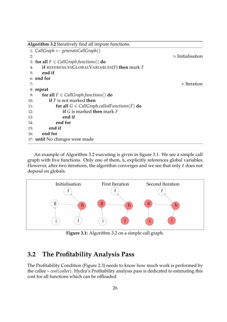
Algorithm 3.2 Iteratively find all impure functions.1: CallGraph← generateCallGraph()2: . Initialisation3: for all F ∈ CallGraph.functions() do4: if REFERENCESGLOBALVARIABLES(F) then mark F5: end if6: end for7: . Iteration8: repeat9: for all F ∈ CallGraph.functions() do
10: if F is not marked then11: for all G ∈ CallGraph.calledFunctions(F) do12: if G is marked then mark F13: end if14: end for15: end if16: end for17: until No changes were made
An example of Algorithm 3.2 executing is given in figure 3.1. We see a simple callgraph with five functions. Only one of them, h, explicitly references global variables.However, after two iterations, the algorithm converges and we see that only f does notdepend on globals.
f
g h
i j
Initialisationf
g h
i j
First Iterationf
g h
i j
Second Iteration
Figure 3.1: Algorithm 3.2 on a simple call graph.
3.2 The Profitability Analysis Pass
The Profitability Condition (Figure 2.3) needs to know how much work is performed bythe callee – cost(callee). Hydra’s Profitability analysis pass is dedicated to estimating thiscost for all functions which can be offloaded.
26
3.2.1 Difficulty of Estimating Profitability
Estimating the cost of a function at compile-time is an inherently difficult task – doingit ‘properly’ is undecidable, due to the Halting Problem. This seems demoralising, butsince the cost of inaccuracy is that the program might run more slowly, we can safely useestimates.
There are several design decisions that need to be established. For a paralleliserwhich never makes the program slower, principles of one-sided error must be employedjudiciously. Such a paralleliser is likely to have a high false negative rate, and commonlymiss profitable parallelisation opportunities. Hydra is not such a paralleliser.
In addition, a balance must be found between good algorithmic complexity and highquality of estimation. While performance of Hydra’s Analyser is not a specific require-ment (§2.3), I decided to aim for asymptotic complexity of quadratic or less. Anythingworse would have limited the tests I could reasonably perform in §4.
A goal for Hydra is target independence, but this has the consequence that theheuristics are of inherently lower quality than ones which have knowledge of a specificplatform. I tried to be optimistic about capabilities of the target so that false positives areminimised. For example, it is assumed that branches never cause a stall.
3.2.2 The First Heuristic
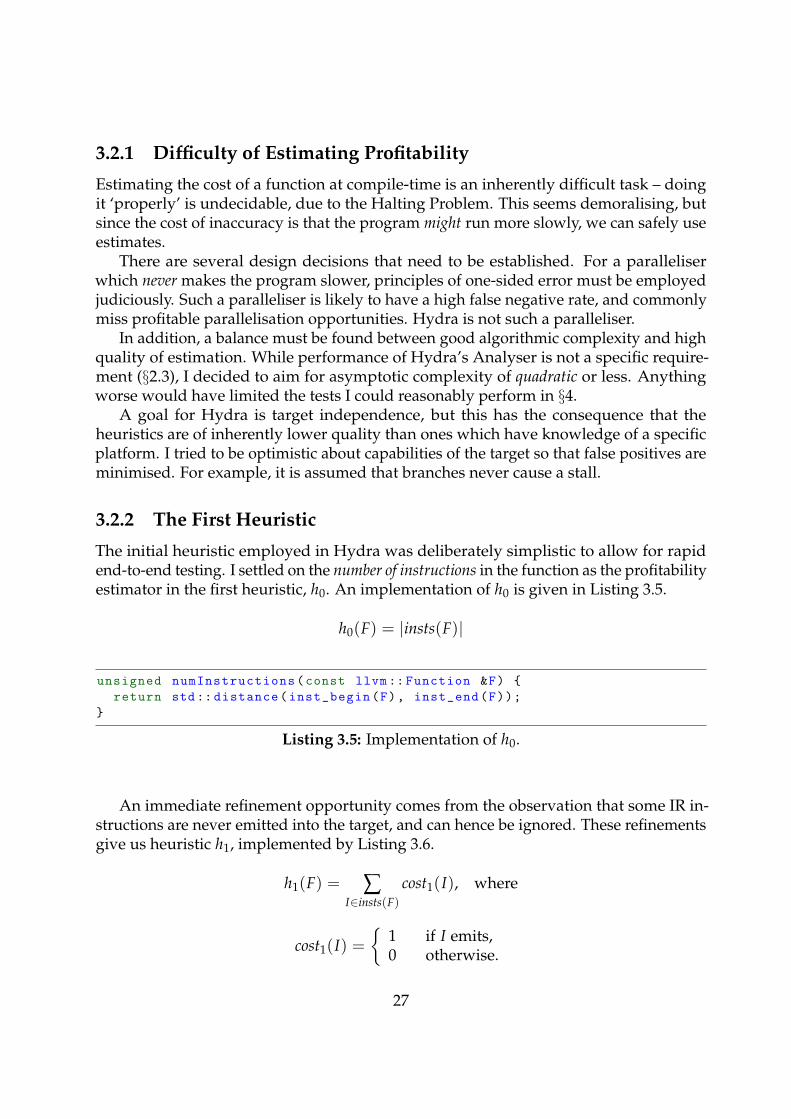
The initial heuristic employed in Hydra was deliberately simplistic to allow for rapidend-to-end testing. I settled on the number of instructions in the function as the profitabilityestimator in the first heuristic, h0. An implementation of h0 is given in Listing 3.5.
h0(F) = |insts(F)|
unsigned numInstructions(const llvm:: Function &F) {
return std:: distance(inst_begin(F), inst_end(F));
}
Listing 3.5: Implementation of h0.
An immediate refinement opportunity comes from the observation that some IR in-structions are never emitted into the target, and can hence be ignored. These refinementsgive us heuristic h1, implemented by Listing 3.6.
h1(F) = ∑I∈insts(F)
cost1(I), where
cost1(I) ={
1 if I emits,0 otherwise.
27
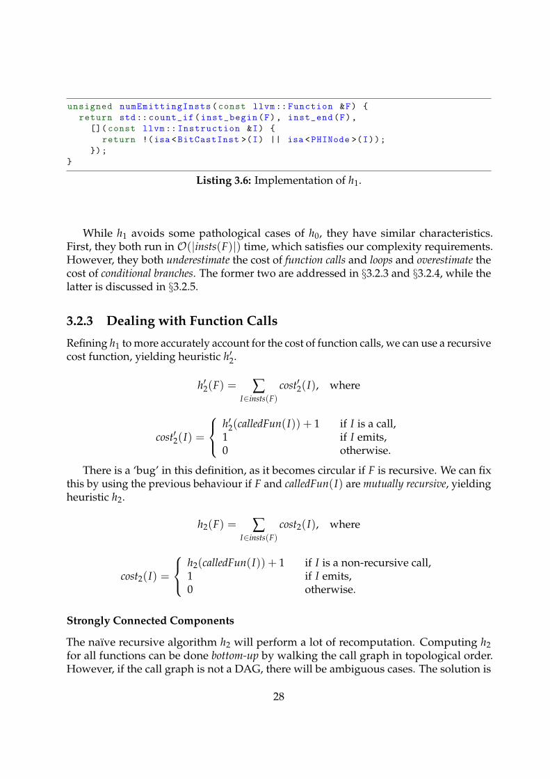
unsigned numEmittingInsts(const llvm:: Function &F) {
return std:: count_if(inst_begin(F), inst_end(F),
[]( const llvm:: Instruction &I) {
return !(isa <BitCastInst >(I) || isa <PHINode >(I));
});
}
Listing 3.6: Implementation of h1.
While h1 avoids some pathological cases of h0, they have similar characteristics.First, they both run in O(|insts(F)|) time, which satisfies our complexity requirements.However, they both underestimate the cost of function calls and loops and overestimate thecost of conditional branches. The former two are addressed in §3.2.3 and §3.2.4, while thelatter is discussed in §3.2.5.
3.2.3 Dealing with Function Calls
Refining h1 to more accurately account for the cost of function calls, we can use a recursivecost function, yielding heuristic h′2.
h′2(F) = ∑I∈insts(F)
cost′2(I), where
cost′2(I) =
h′2(calledFun(I)) + 1 if I is a call,1 if I emits,0 otherwise.
There is a ‘bug’ in this definition, as it becomes circular if F is recursive. We can fixthis by using the previous behaviour if F and calledFun(I) are mutually recursive, yieldingheuristic h2.
h2(F) = ∑I∈insts(F)
cost2(I), where
cost2(I) =
h2(calledFun(I)) + 1 if I is a non-recursive call,1 if I emits,0 otherwise.
Strongly Connected Components
The naıve recursive algorithm h2 will perform a lot of recomputation. Computing h2for all functions can be done bottom-up by walking the call graph in topological order.However, if the call graph is not a DAG, there will be ambiguous cases. The solution is
28
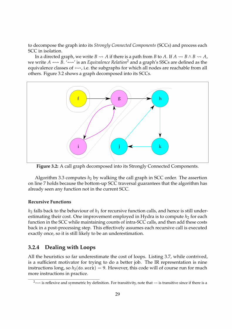
to decompose the graph into its Strongly Connected Components (SCCs) and process eachSCC in isolation.
In a directed graph, we write B A if there is a path from B to A. If A B∧ B A,we write A! B. ‘!’ is an Equivalence Relation2 and a graph’s SSCs are defined as theequivalence classes of!, i.e. the subgraphs for which all nodes are reachable from allothers. Figure 3.2 shows a graph decomposed into its SCCs.
f
kji
g h
Figure 3.2: A call graph decomposed into its Strongly Connected Components.
Algorithm 3.3 computes h2 by walking the call graph in SCC order. The assertionon line 7 holds because the bottom-up SCC traversal guarantees that the algorithm hasalready seen any function not in the current SCC.
Recursive Functions
h2 falls back to the behaviour of h1 for recursive function calls, and hence is still under-estimating their cost. One improvement employed in Hydra is to compute h2 for eachfunction in the SCC while maintaining counts of intra-SCC calls, and then add these costsback in a post-processing step. This effectively assumes each recursive call is executedexactly once, so it is still likely to be an underestimation.
3.2.4 Dealing with Loops
All the heuristics so far underestimate the cost of loops. Listing 3.7, while contrived,is a sufficient motivator for trying to do a better job. The IR representation is nineinstructions long, so h2(do work) = 9. However, this code will of course run for muchmore instructions in practice.
2! is reflexive and symmetric by definition. For transitivity, note that is transitive since if there is a
29
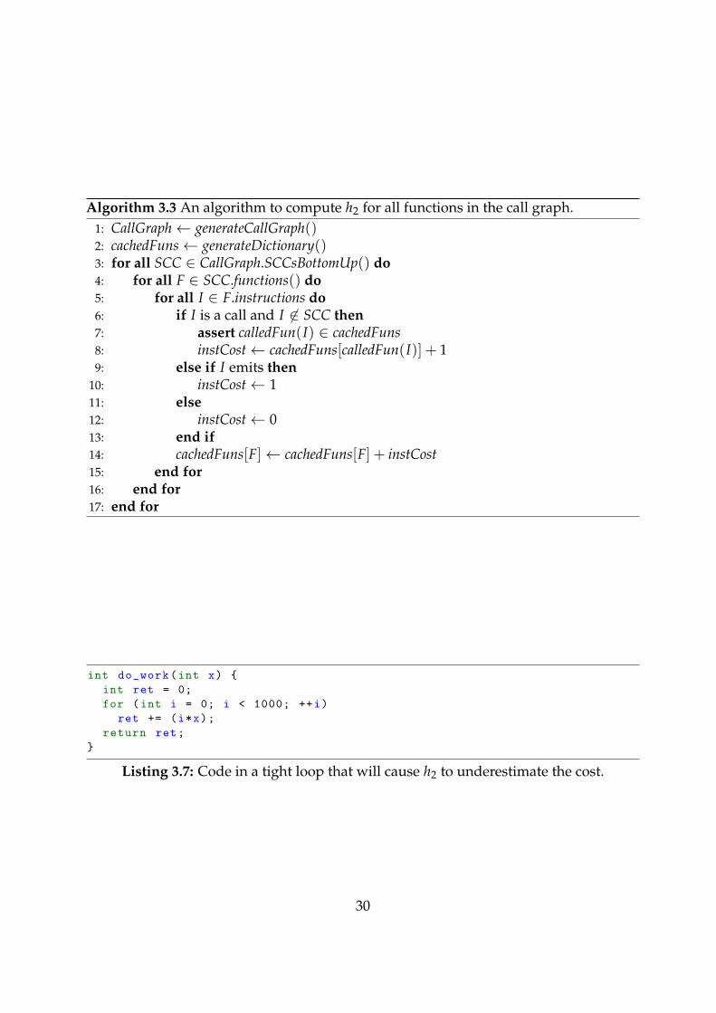
Algorithm 3.3 An algorithm to compute h2 for all functions in the call graph.1: CallGraph← generateCallGraph()2: cachedFuns← generateDictionary()3: for all SCC ∈ CallGraph.SCCsBottomUp() do4: for all F ∈ SCC.functions() do5: for all I ∈ F.instructions do6: if I is a call and I 6∈ SCC then7: assert calledFun(I) ∈ cachedFuns8: instCost← cachedFuns[calledFun(I)] + 19: else if I emits then
10: instCost← 111: else12: instCost← 013: end if14: cachedFuns[F]← cachedFuns[F] + instCost15: end for16: end for17: end for
int do_work(int x) {
int ret = 0;
for (int i = 0; i < 1000; ++i)
ret += (i*x);
return ret;
}
Listing 3.7: Code in a tight loop that will cause h2 to underestimate the cost.
30
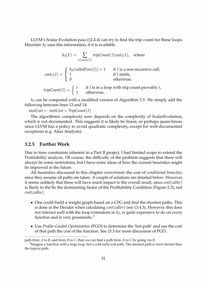
LLVM’s Scalar Evolution pass (§2.4.4) can try to find the trip count for these loops.Heuristic h3 uses this information, if it is available.
h3(F) = ∑I∈insts(F)
tripCount(I)cost3(I), where
cost3(I) =
h3(calledFun(I)) + 1 if I is a non-recursive call,1 if I emits,0 otherwise.
tripCount(I) ={
t if I is in a loop with trip count provably t,1 otherwise.
h3 can be computed with a modified version of Algorithm 3.3. We simply add thefollowing between lines 13 and 14:
instCost← instCost× TripCount(I)The algorithmic complexity now depends on the complexity of ScalarEvolution,
which is not documented. This suggests it is likely be linear, or perhaps quasi-linear,since LLVM has a policy to avoid quadratic complexity, except for well-documentedexceptions (e.g. Alias Analysis).
3.2.5 Further Work
Due to time constraints inherent in a Part II project, I had limited scope to extend theProfitability analysis. Of course, the difficulty of the problem suggests that there willalways be some restrictions, but I have some ideas of how the current heuristics mightbe improved in the future.
All heuristics discussed in this chapter overestimate the cost of conditional branches,since they assume all paths are taken. A couple of solutions are detailed below. However,it seems unlikely that these will have much impact to the overall result, since cost(caller)is likely to the be the dominating factor of the Profitability Condition (Figure 2.3), notcost(callee).
• One could build a weight graph based on a CFG and find the shortest paths. Thisis done in the Decider when calculating cost(caller) (see §3.4.3). However, this doesnot interact well with the loop extensions in h3, is quite expensive to do on everyfunction and is very pessimistic.3
• Use Profile-Guided Optimisation (PGO) to determine the ‘hot-path’ and use the costof that path the cost of the function. See §5.3 for more discussion of PGO.
path from A to B, and from B to C, then we can find a path from A to C by going via B.3Imagine a function with a large loop, but a cold early-exit path. The shortest path is much shorter than
the typical path.
31
As mentioned in §3.2.1, Hydra’s heuristics are weaker than ones which are target-aware. Using a ‘swappable’ version would allow target-aware heuristics to be used whereavailable, whilst maintaining the general heuristic for unknown targets.
3.3 The JoinPoints Analysis Pass
Finding where to join with an offloaded function is a mission-critical component ofHydra – getting this wrong results in correctness being is almost certainly lost. At thesame time, we have a desire to place the join as late as is safely possible, to allow moreparallelism to be extracted. Hydra distinguishes between exactly-once (§3.3.2) and at-least-once (§3.3.3) joining. We will see that the latter allows us to achieve better results than theformer.
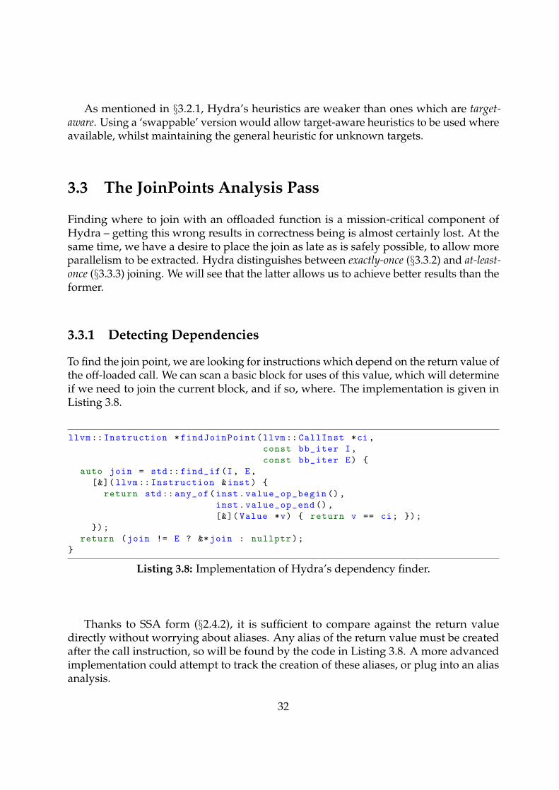
3.3.1 Detecting Dependencies
To find the join point, we are looking for instructions which depend on the return value ofthe off-loaded call. We can scan a basic block for uses of this value, which will determineif we need to join the current block, and if so, where. The implementation is given inListing 3.8.
llvm:: Instruction *findJoinPoint(llvm:: CallInst *ci ,
const bb_iter I,
const bb_iter E) {
auto join = std:: find_if(I, E,
[&]( llvm:: Instruction &inst) {
return std:: any_of(inst.value_op_begin (),
inst.value_op_end (),
[&]( Value *v) { return v == ci; });
});
return (join != E ? &*join : nullptr);
}
Listing 3.8: Implementation of Hydra’s dependency finder.
Thanks to SSA form (§2.4.2), it is sufficient to compare against the return valuedirectly without worrying about aliases. Any alias of the return value must be createdafter the call instruction, so will be found by the code in Listing 3.8. A more advancedimplementation could attempt to track the creation of these aliases, or plug into an aliasanalysis.
32
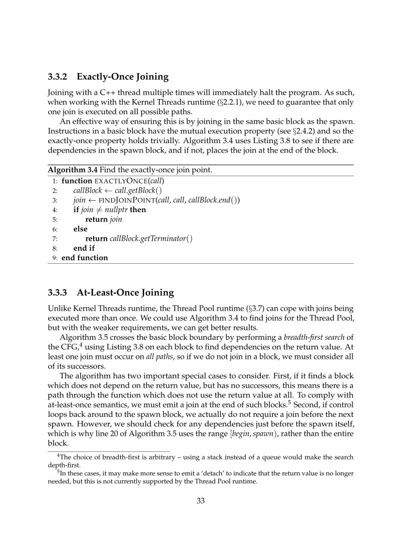
3.3.2 Exactly-Once Joining
Joining with a C++ thread multiple times will immediately halt the program. As such,when working with the Kernel Threads runtime (§2.2.1), we need to guarantee that onlyone join is executed on all possible paths.
An effective way of ensuring this is by joining in the same basic block as the spawn.Instructions in a basic block have the mutual execution property (see §2.4.2) and so theexactly-once property holds trivially. Algorithm 3.4 uses Listing 3.8 to see if there aredependencies in the spawn block, and if not, places the join at the end of the block.
Algorithm 3.4 Find the exactly-once join point.1: function EXACTLYONCE(call)2: callBlock← call.getBlock()3: join← FINDJOINPOINT(call, call, callBlock.end())4: if join 6= nullptr then5: return join6: else7: return callBlock.getTerminator()8: end if9: end function
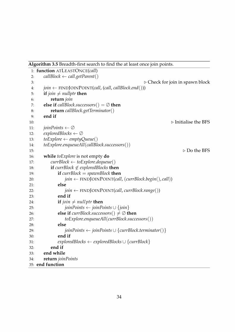
3.3.3 At-Least-Once Joining
Unlike Kernel Threads runtime, the Thread Pool runtime (§3.7) can cope with joins beingexecuted more than once. We could use Algorithm 3.4 to find joins for the Thread Pool,but with the weaker requirements, we can get better results.
Algorithm 3.5 crosses the basic block boundary by performing a breadth-first search ofthe CFG,4 using Listing 3.8 on each block to find dependencies on the return value. Atleast one join must occur on all paths, so if we do not join in a block, we must consider allof its successors.
The algorithm has two important special cases to consider. First, if it finds a blockwhich does not depend on the return value, but has no successors, this means there is apath through the function which does not use the return value at all. To comply withat-least-once semantics, we must emit a join at the end of such blocks.5 Second, if controlloops back around to the spawn block, we actually do not require a join before the nextspawn. However, we should check for any dependencies just before the spawn itself,which is why line 20 of Algorithm 3.5 uses the range [begin, spawn), rather than the entireblock.
4The choice of breadth-first is arbitrary – using a stack instead of a queue would make the searchdepth-first.
5In these cases, it may make more sense to emit a ‘detach’ to indicate that the return value is no longerneeded, but this is not currently supported by the Thread Pool runtime.
33
Algorithm 3.5 Breadth-first search to find the at least once join points.1: function ATLEASTONCE(call)2: callBlock← call.getParent()3: . Check for join in spawn block4: join← FINDJOINPOINT(call, (call, callBlock.end()))5: if join 6= nullptr then6: return join7: else if callBlock.successors() = ∅ then8: return callBlock.getTerminator()9: end if
10: . Initialise the BFS11: joinPoints← ∅12: exploredBlocks← ∅13: toExplore← emptyQueue()14: toExplore.enqueueAll(callBlock.successors())15: . Do the BFS16: while toExplore is not empty do17: currBlock← toExplore.dequeue()18: if currBlock 6∈ exploredBlocks then19: if currBlock = spawnBlock then20: join← FINDJOINPOINT(call, (currBlock.begin(), call))21: else22: join← FINDJOINPOINT(call, currBlock.range())23: end if24: if join 6= nullptr then25: joinPoints← joinPoints∪ {join}26: else if currBlock.successors() 6= ∅ then27: toExplore.enqueueAll(currBlock.successors())28: else29: joinPoints← joinPoints∪ {currBlock.terminator()}30: end if31: exploredBlocks← exploredBlocks∪ {currBlock}32: end if33: end while34: return joinPoints35: end function
34
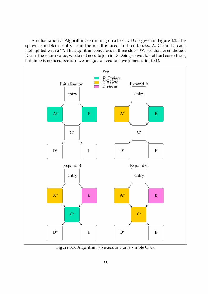
An illustration of Algorithm 3.5 running on a basic CFG is given in Figure 3.3. Thespawn is in block ‘entry’, and the result is used in three blocks, A, C and D, eachhighlighted with a ‘*’. The algorithm converges in three steps. We see that, even thoughD uses the return value, we do not need to join in D. Doing so would not hurt correctness,but there is no need because we are guaranteed to have joined prior to D.
KeyTo ExploreJoin Here
entry
B
C*
D* E
A*
Expand A
entry
B
C*
D* E
A*
Expand C
entry
B
C*
D* E
A*
Expand B
entry
B
C*
D* E
A*
Initialisation Explored
Figure 3.3: Algorithm 3.5 executing on a simple CFG.
35
3.4 The Decider Analysis Pass
At this point in the process, the Analyser has computed a lot of information about theprogram – which functions can be safely spawned, an approximation of their cost andwhere we can safely join with them, if they were to be offloaded. We almost have enoughto make the final decision using the Profitability Condition (Figure 2.3) and decide whichcalls should be offloaded. The Decider will combine all the information we have to makethis final decision before Hydra passes control to the Transformer.
3.4.1 The Missing Piece
To compute the Profitability Condition (Figure 2.3), we require cost(caller), cost(callee)and cost(spawn), the second of which has already been computed by Profitability (§3.2),and the last is found ahead of time empirically (see §4.3). All that remains is to computecost(caller), the amount of work which can safely be done in parallel with the callee. Assuch, we require a heuristic which estimates the cost of the work between the spawn andthe join(s).
The heuristic I use in the Decider is similar to h2 (§3.2.3). h2 was a refinement whichincluded the cost of called functions. Since the Decider sees the output from Profitability,it already knows the costs for all functions which may be called.
An h3-style heuristic (§3.2.4) was not used because there is added complexity to loopcost when we want to know the cost between two points in the function rather than thewhole function.6 Note that since h3 is used by Profitability, it is also used in the Deciderfor the cost of function calls.
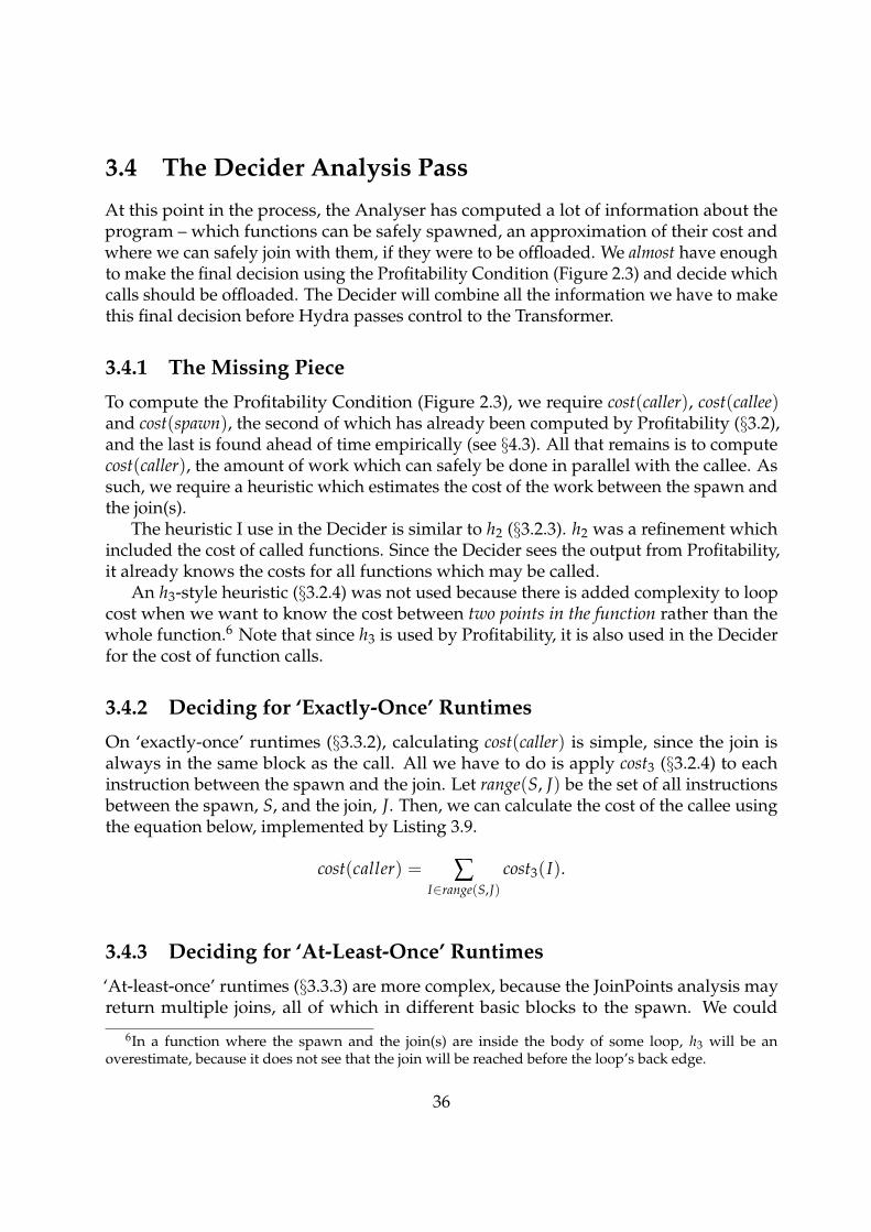
3.4.2 Deciding for ‘Exactly-Once’ Runtimes
On ‘exactly-once’ runtimes (§3.3.2), calculating cost(caller) is simple, since the join isalways in the same block as the call. All we have to do is apply cost3 (§3.2.4) to eachinstruction between the spawn and the join. Let range(S, J) be the set of all instructionsbetween the spawn, S, and the join, J. Then, we can calculate the cost of the callee usingthe equation below, implemented by Listing 3.9.
cost(caller) = ∑I∈range(S,J)
cost3(I).
3.4.3 Deciding for ‘At-Least-Once’ Runtimes
‘At-least-once’ runtimes (§3.3.3) are more complex, because the JoinPoints analysis mayreturn multiple joins, all of which in different basic blocks to the spawn. We could
6In a function where the spawn and the join(s) are inside the body of some loop, h3 will be anoverestimate, because it does not see that the join will be reached before the loop’s back edge.
36
int countInstructions(bb_citer first , bb_citer last ,
const Profitability &Profit) {
int count = std:: accumulate(first , last , 0,
[&]( int runningTotal , const llvm:: Instruction &i) {
int extraInsts{ 1 };
if (auto *ci = dyn_cast <CallInst >(&i)) {
extraInsts += Profit.getFunStats(
*ci ->getCalledFunction ())->totalCost;
}
return runningTotal + extraInsts;
});
return count;
}
Listing 3.9: Calculating cost(caller) for ‘exactly-once’ runtimes.
proceed by applying cost3 to every possible instruction between the spawn and thejoin. However, this is likely to be an overestimate of the cost, and we generally want toavoid overestimating cost(caller) since it is often the deciding factor in the ProfitabilityCondition (Figure 2.3).
A conservative alternative used in Hydra finds the shortest paths to the joins. We cando this by building a weighted graph, where the nodes represent instructions of interest,and the weights represent the h2 cost of the path. Then Dijkstra’s Algorithm [11] canbe used to efficiently compute the shortest paths. The only requirement of Dijkstrais that the graph must not contain negative weights, which is fine since h2 is alwaysnon-negative.
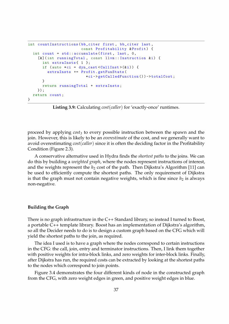
Building the Graph
There is no graph infrastructure in the C++ Standard library, so instead I turned to Boost,a portable C++ template library. Boost has an implementation of Dijkstra’s algorithm,so all the Decider needs to do is to design a custom graph based on the CFG which willyield the shortest paths to the join, as required.
The idea I used is to have a graph where the nodes correspond to certain instructionsin the CFG: the call, join, entry and terminator instructions. Then, I link them togetherwith positive weights for intra-block links, and zero weights for inter-block links. Finally,after Dijkstra has run, the required costs can be extracted by looking at the shortest pathsto the nodes which correspond to join points.
Figure 3.4 demonstrates the four different kinds of node in the constructed graphfrom the CFG, with zero weight edges in green, and positive weight edges in blue.
37
Constructed Graph
Entry0
Call
Terminator0
CFG
P0 Pm. . .
Entry1
Terminator1
Entry2
Join
S0 Sn. . .
. . .P0 Pm
Entry0
Call
Terminator0
Entry1 Entry2
Terminator1 Join
S0 Sn. . .
KeyZero-Cost Linkh2-Cost Link
Figure 3.4: Illustration of the CFG to custom graph conversion.
38
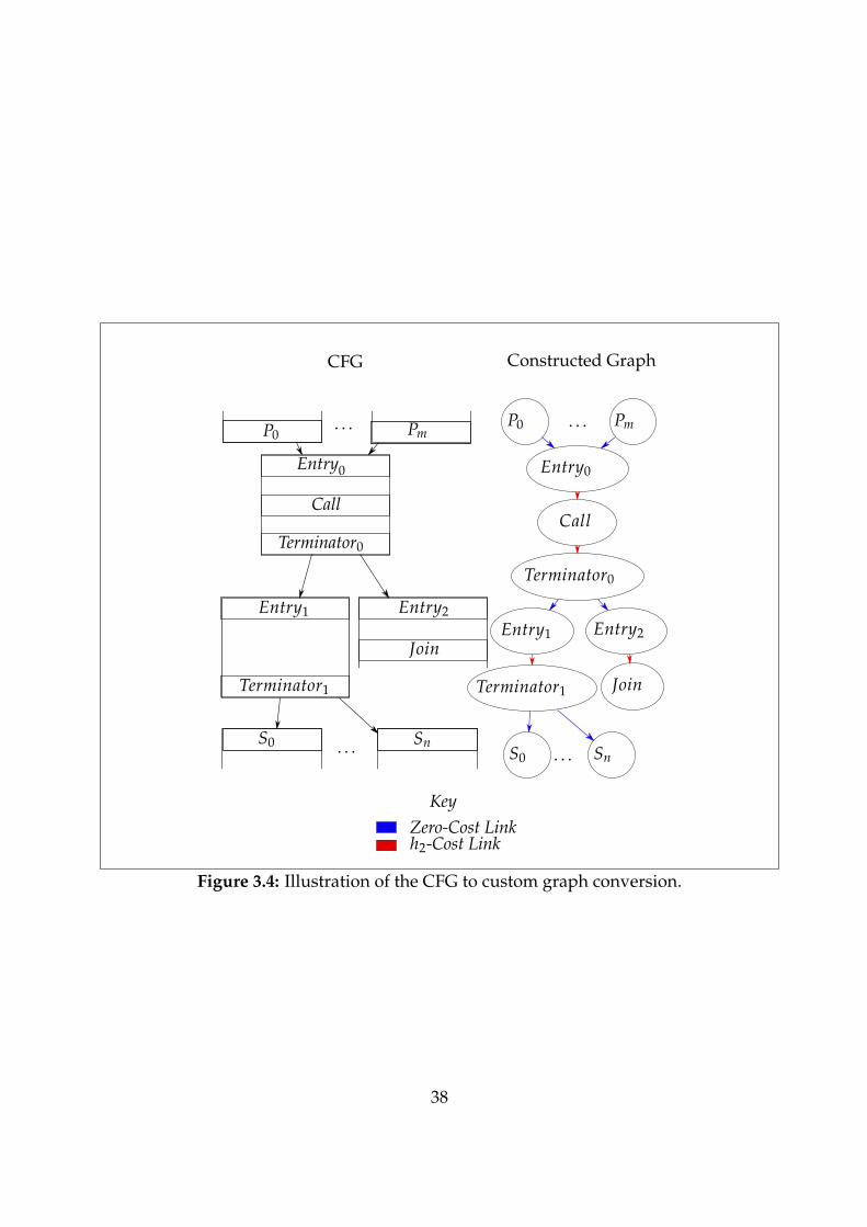
Accumulating the Results
Now that we have the costs of the shortest paths to each join, the question remains asto how we combine all of these to estimate cost(caller). Hydra supports three differentmethods. Denote the set of the shortest paths as paths, and the cost of a path, p, as cost(p).Then, we can write down our various approaches for estimating cost(caller).
There is the optimist’s approach:
cost(caller) = maxp∈paths
{cost(p)}
The pessimist’s approach:
cost(caller) = minp∈paths
{cost(p)}
And the realist’s approach:
cost(caller) =1
|paths| ∑p∈paths
cost(p)
Actually, the ‘right’ way to do this is by taking into account path probabilities, andthen calculating cost(caller) as an expected value, as below. However, calculating P(p)requires Profile-Guided Optimisation, which is one of the features Hydra might support infuture work (see §5.3).
cost(caller) = ∑p∈paths
P(p)cost(p).
3.5 The MakeSpawnable Transformation Pass
At this point in the process, the Analyser has completed. It has done the hard work, andHydra knows which functions it wants to offload. However, there are a few interfaceconcerns that it has to address before we can go ahead and replace the call with arequest to spawn. A new function signature needs to be synthesised to conform with thespawning APIs of our supported runtimes, and it is the MakeSpawnable transformation’sjob to do this.
3.5.1 Statement of the Problem
Let us first consider the problems which MakeSpawnable must solve. Most of the thesecome from the Kernel Threads runtime (§2.2.1), but their solution allows simplificationof the Thread Pool runtime (see §3.7).
All the functions that Hydra would like to spawn use return values to get theirresults back to the caller. The alternative would be to use an ‘out-parameter’, but this
39
is banned since Hydra forbids functions from using pointer arguments. This causes aslight problem: when we create an std::thread object with a function to execute, thereturn value is ignored. To get around this, we require the synthesised function to returnvia an out-parameter instead. I describe this mechanism in §3.5.2.
Another concern is that the function to be offloaded may have parameters of user-defined type. This a problem because std::thread deals with user-defined types usingvariadic templates, but the C++ template machinery is not available at the LLVM IR levelof the compiler. The solution is to pass all arguments by void* pointer in the synthesisedfunction, which is explained in §3.5.3.
3.5.2 Dealing with Return Values
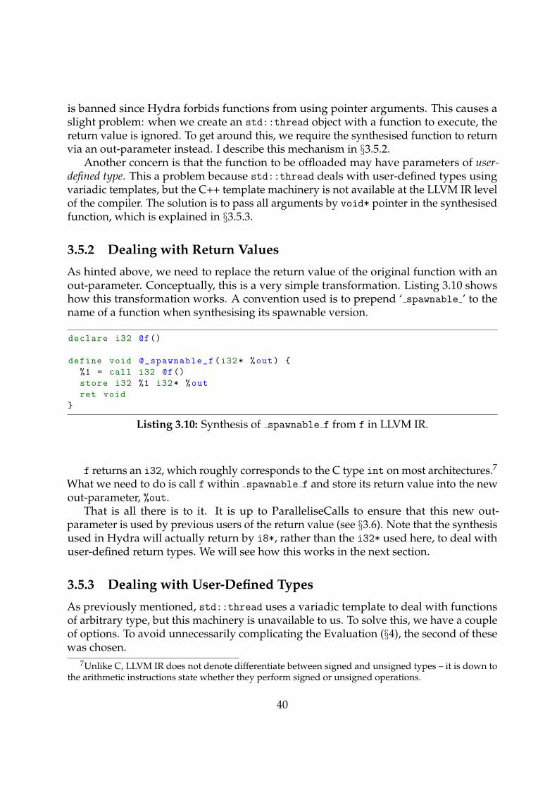
As hinted above, we need to replace the return value of the original function with anout-parameter. Conceptually, this is a very simple transformation. Listing 3.10 showshow this transformation works. A convention used is to prepend ‘ spawnable ’ to thename of a function when synthesising its spawnable version.
declare i32 @f()
define void @_spawnable_f(i32* %out) {
%1 = call i32 @f()
store i32 %1 i32* %out
ret void
}
Listing 3.10: Synthesis of spawnable f from f in LLVM IR.
f returns an i32, which roughly corresponds to the C type int on most architectures.7
What we need to do is call f within spawnable f and store its return value into the newout-parameter, %out.
That is all there is to it. It is up to ParalleliseCalls to ensure that this new out-parameter is used by previous users of the return value (see §3.6). Note that the synthesisused in Hydra will actually return by i8*, rather than the i32* used here, to deal withuser-defined return types. We will see how this works in the next section.
3.5.3 Dealing with User-Defined Types
As previously mentioned, std::thread uses a variadic template to deal with functionsof arbitrary type, but this machinery is unavailable to us. To solve this, we have a coupleof options. To avoid unnecessarily complicating the Evaluation (§4), the second of thesewas chosen.
7Unlike C, LLVM IR does not denote differentiate between signed and unsigned types – it is down tothe arithmetic instructions state whether they perform signed or unsigned operations.
40
• Hydra could emit a list of template instantiations which it would like someone toinstantiate and link in. While this approach has its advantages, it is inconvenientand makes compilation more complex, especially since LLVM has no mechanismto do this.
• One could instantiate all the templates needed with void*,8 and then have Hydraemit casts in the synthesised function. This does mean that primitive types suffer apenalty since they need to be placed on the stack rather than passed in registers.9
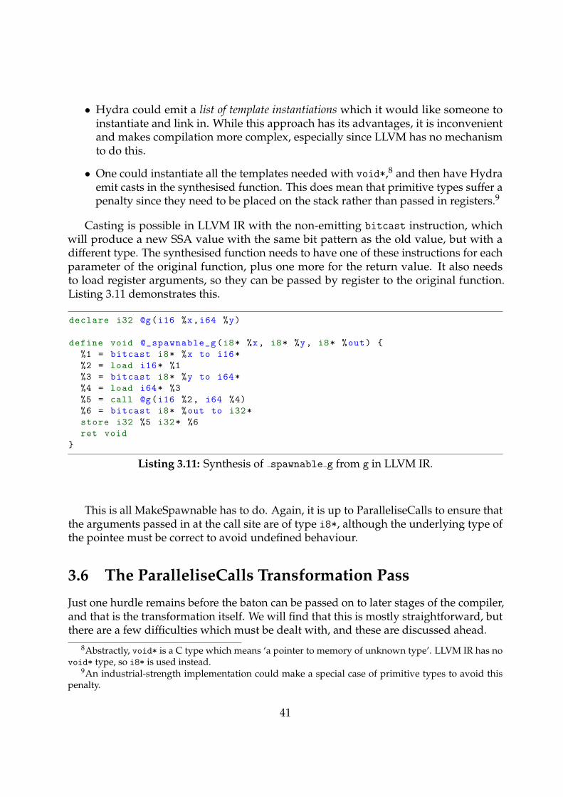
Casting is possible in LLVM IR with the non-emitting bitcast instruction, whichwill produce a new SSA value with the same bit pattern as the old value, but with adifferent type. The synthesised function needs to have one of these instructions for eachparameter of the original function, plus one more for the return value. It also needsto load register arguments, so they can be passed by register to the original function.Listing 3.11 demonstrates this.
declare i32 @g(i16 %x,i64 %y)
define void @_spawnable_g(i8* %x, i8* %y, i8* %out) {
%1 = bitcast i8* %x to i16*
%2 = load i16* %1
%3 = bitcast i8* %y to i64*
%4 = load i64* %3
%5 = call @g(i16 %2, i64 %4)
%6 = bitcast i8* %out to i32*
store i32 %5 i32* %6
ret void
}
Listing 3.11: Synthesis of spawnable g from g in LLVM IR.
This is all MakeSpawnable has to do. Again, it is up to ParalleliseCalls to ensure thatthe arguments passed in at the call site are of type i8*, although the underlying type ofthe pointee must be correct to avoid undefined behaviour.
3.6 The ParalleliseCalls Transformation Pass
Just one hurdle remains before the baton can be passed on to later stages of the compiler,and that is the transformation itself. We will find that this is mostly straightforward, butthere are a few difficulties which must be dealt with, and these are discussed ahead.
8Abstractly, void* is a C type which means ‘a pointer to memory of unknown type’. LLVM IR has novoid* type, so i8* is used instead.
9An industrial-strength implementation could make a special case of primitive types to avoid thispenalty.
41
3.6.1 Adding the Runtime API to the Module
A lot of the work presented ahead is quite dependent on the target runtime in question.Recall that the two supported runtimes of this project are Kernel Threads and theThread Pool. ParalleliseCalls needs to add the signatures for the APIs we require into theLLVM IR module so that we can emit the spawns and joins. Their implementation willbe linked in later.
Kernel Threads API
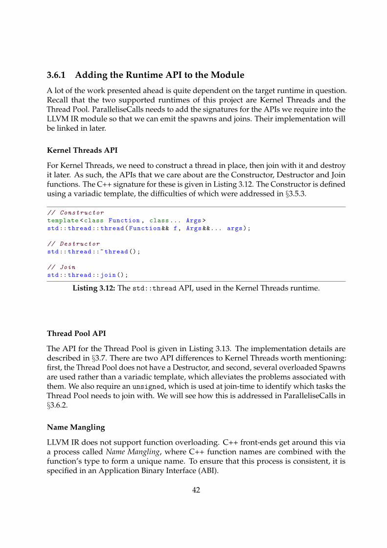
For Kernel Threads, we need to construct a thread in place, then join with it and destroyit later. As such, the APIs that we care about are the Constructor, Destructor and Joinfunctions. The C++ signature for these is given in Listing 3.12. The Constructor is definedusing a variadic template, the difficulties of which were addressed in §3.5.3.
// Constructor
template <class Function , class ... Args >
std:: thread :: thread(Function && f, Args &&... args);
// Destructor
std:: thread ::~ thread ();
// Join
std:: thread ::join();
Listing 3.12: The std::thread API, used in the Kernel Threads runtime.
Thread Pool API
The API for the Thread Pool is given in Listing 3.13. The implementation details aredescribed in §3.7. There are two API differences to Kernel Threads worth mentioning:first, the Thread Pool does not have a Destructor, and second, several overloaded Spawnsare used rather than a variadic template, which alleviates the problems associated withthem. We also require an unsigned, which is used at join-time to identify which tasks theThread Pool needs to join with. We will see how this is addressed in ParalleliseCalls in§3.6.2.
Name Mangling
LLVM IR does not support function overloading. C++ front-ends get around this viaa process called Name Mangling, where C++ function names are combined with thefunction’s type to form a unique name. To ensure that this process is consistent, it isspecified in an Application Binary Interface (ABI).
42
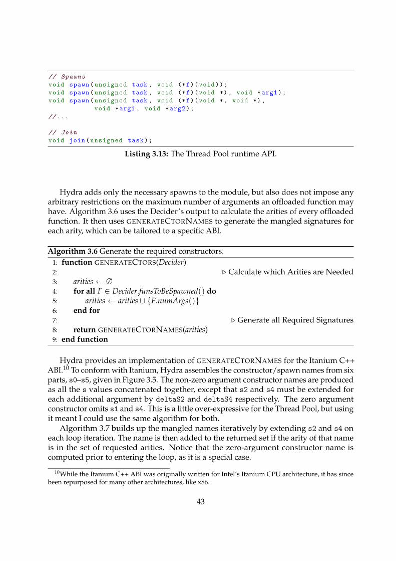
// Spawns
void spawn(unsigned task , void (*f)(void));
void spawn(unsigned task , void (*f)(void *), void *arg1);
void spawn(unsigned task , void (*f)(void *, void *),
void *arg1 , void *arg2);
//...
// Join
void join(unsigned task);
Listing 3.13: The Thread Pool runtime API.
Hydra adds only the necessary spawns to the module, but also does not impose anyarbitrary restrictions on the maximum number of arguments an offloaded function mayhave. Algorithm 3.6 uses the Decider’s output to calculate the arities of every offloadedfunction. It then uses GENERATECTORNAMES to generate the mangled signatures foreach arity, which can be tailored to a specific ABI.
Algorithm 3.6 Generate the required constructors.1: function GENERATECTORS(Decider)2: . Calculate which Arities are Needed3: arities← ∅4: for all F ∈ Decider.funsToBeSpawned() do5: arities← arities∪ {F.numArgs()}6: end for7: . Generate all Required Signatures8: return GENERATECTORNAMES(arities)9: end function
Hydra provides an implementation of GENERATECTORNAMES for the Itanium C++ABI.10 To conform with Itanium, Hydra assembles the constructor/spawn names from sixparts, s0–s5, given in Figure 3.5. The non-zero argument constructor names are producedas all the s values concatenated together, except that s2 and s4 must be extended foreach additional argument by deltaS2 and deltaS4 respectively. The zero argumentconstructor omits s1 and s4. This is a little over-expressive for the Thread Pool, but usingit meant I could use the same algorithm for both.
Algorithm 3.7 builds up the mangled names iteratively by extending s2 and s4 oneach loop iteration. The name is then added to the returned set if the arity of that nameis in the set of requested arities. Notice that the zero-argument constructor name iscomputed prior to entering the loop, as it is a special case.
10While the Itanium C++ ABI was originally written for Intel’s Itanium CPU architecture, it has sincebeen repurposed for many other architectures, like x86.
43
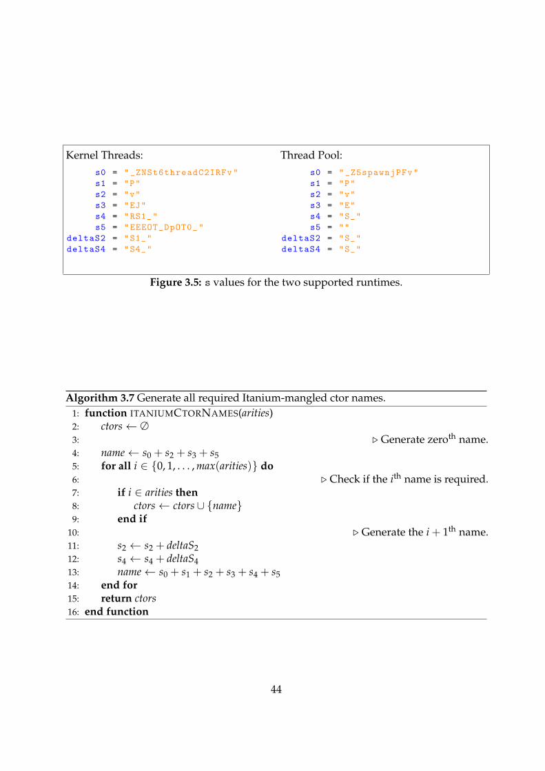
Kernel Threads:s0 = "_ZNSt6threadC2IRFv"
s1 = "P"
s2 = "v"
s3 = "EJ"
s4 = "RS1_"
s5 = "EEEOT_DpOT0_"
deltaS2 = "S1_"
deltaS4 = "S4_"
Thread Pool:s0 = "_Z5spawnjPFv"
s1 = "P"
s2 = "v"
s3 = "E"
s4 = "S_"
s5 = ""
deltaS2 = "S_"
deltaS4 = "S_"
Figure 3.5: s values for the two supported runtimes.
Algorithm 3.7 Generate all required Itanium-mangled ctor names.1: function ITANIUMCTORNAMES(arities)2: ctors← ∅3: . Generate zeroth name.4: name← s0 + s2 + s3 + s55: for all i ∈ {0, 1, . . . , max(arities)} do6: . Check if the ith name is required.7: if i ∈ arities then8: ctors← ctors∪ {name}9: end if
10: . Generate the i + 1th name.11: s2 ← s2 + deltaS212: s4 ← s4 + deltaS413: name← s0 + s1 + s2 + s3 + s4 + s514: end for15: return ctors16: end function
44
3.6.2 Dealing with the ‘Task’ ID in the Thread Pool
The Thread Pool API (Listing 3.13), requires an unsigned for spawning and joining sothat the Pool can identify which tasks need to be joined with at join-time. It is perfectlysafe to generate a random constant at compile-time and use that, since if two task IDsclash, we will simply join with tasks a little early in the Thread Pool and we only have aperformance problem, not a correctness problem.
C++ provides facilities for generating fast, high quality random data. Hydra uses theincluded Mersenne Twister generator [12]. Mersenne Twister is fast, deterministic (whichis useful for debugging) and extremely high-quality. Hydra uses std::random device toseed the twister, which is designed to produce unpredictable (sometimes cryptographi-cally secure) random data, but can be quite slow.
3.6.3 Switching the Uses of the Return Value
Once the API signatures have been added to the module, one difficulty remains – Hydramust replace all the previous uses of the return value with the new return value.
Loading the Return Value
Recall that the spawnable version of our function will get its return value to us by storingit into its out parameter when it has finished. As such, it is vital that we load it afterjoining with the function.
Hydra could load the value at the join(s), and swap the uses of the return valuewith this newly loaded value, but this becomes complex if there is more than one join.Fortunately, LLVM encourages passes to be liberal with the number of loads used, andallow later stages of the compiler (and even the hardware) to optimise redundant loads.This is the approach taken by Hydra.
Finding all the Uses of a Value
Hydra finds all the uses of the return value, and replaces them with a freshly emittedload of the offloaded function’s out parameter. Rather than searching the CFG manually,LLVM provides a use iterator to conveniently iterate over all the uses of an SSA value.The implementation is given in Listing 3.14. Within the transform on line 10, if thevalue is the call instruction, then it is using the return value and we swap it with theload generated on line 8. Otherwise, we return what we were given to the effect of notmodifying the value.
3.7 The Thread Pool
Once the compiler has emitted the target code, sprinkled with spawn and join API calls,all that remains is to run it. For the Kernel Threads runtime, no more work is required,
45
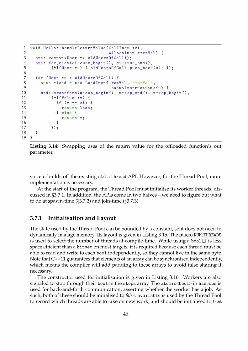
1 void Hello:: handleReturnValue(CallInst *ci ,
2 AllocaInst *retVal) {
3 std::vector <User *> oldUsersOfCall {};
4 std:: for_each(ci ->use_begin (), ci ->use_end (),
5 [&]( User *u) { oldUsersOfCall.push_back(u); });
67 for (User *u : oldUsersOfCall) {
8 auto *load = new LoadInst{ retVal , "retVal",
9 cast <Instruction >(u) };
10 std:: transform(u->op_begin (), u->op_end (), u->op_begin (),
11 [=]( Value *v) {
12 if (v == ci) {
13 return load;
14 } else {
15 return v;
16 }
17 });
18 }
19 }
Listing 3.14: Swapping uses of the return value for the offloaded function’s outparameter.
since it builds off the existing std::thread API. However, for the Thread Pool, moreimplementation is necessary.
At the start of the program, the Thread Pool must initialise its worker threads, dis-cussed in §3.7.1. In addition, the APIs come in two halves – we need to figure out whatto do at spawn-time (§3.7.2) and join-time (§3.7.3).
3.7.1 Initialisation and Layout
The state used by the Thread Pool can be bounded by a constant, so it does not need todynamically manage memory. Its layout is given in Listing 3.15. The macro NUM THREADS
is used to select the number of threads at compile-time. While using a bool[] is lessspace efficient than a bitset on most targets, it is required because each thread must beable to read and write to each bool independently, so they cannot live in the same byte.Note that C++11 guarantees that elements of an array can be synchronised independently,which means the compiler will add padding to these arrays to avoid false sharing ifnecessary.
The constructor used for initialisation is given in Listing 3.16. Workers are alsosignaled to stop through their bool in the stops array. The atomic<bool> in hasJobs isused for back-and-forth communication, asserting whether the worker has a job. Assuch, both of these should be initialised to false. available is used by the Thread Poolto record which threads are able to take on new work, and should be initialised to true.
46
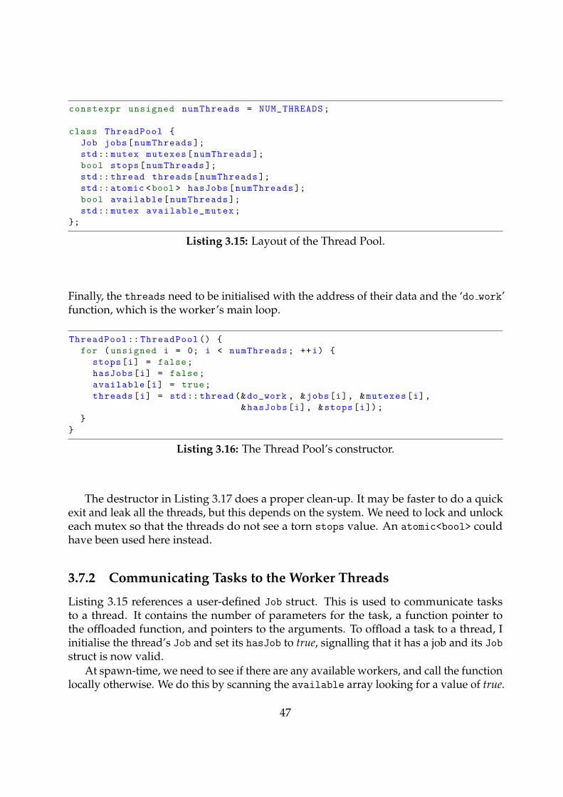
constexpr unsigned numThreads = NUM_THREADS;
class ThreadPool {
Job jobs[numThreads ];
std:: mutex mutexes[numThreads ];
bool stops[numThreads ];
std:: thread threads[numThreads ];
std::atomic <bool > hasJobs[numThreads ];
bool available[numThreads ];
std:: mutex available_mutex;
};
Listing 3.15: Layout of the Thread Pool.
Finally, the threads need to be initialised with the address of their data and the ‘do work’function, which is the worker’s main loop.
ThreadPool :: ThreadPool () {
for (unsigned i = 0; i < numThreads; ++i) {
stops[i] = false;
hasJobs[i] = false;
available[i] = true;
threads[i] = std:: thread (&do_work , &jobs[i], &mutexes[i],
&hasJobs[i], &stops[i]);
}
}
Listing 3.16: The Thread Pool’s constructor.
The destructor in Listing 3.17 does a proper clean-up. It may be faster to do a quickexit and leak all the threads, but this depends on the system. We need to lock and unlockeach mutex so that the threads do not see a torn stops value. An atomic<bool> couldhave been used here instead.
3.7.2 Communicating Tasks to the Worker Threads
Listing 3.15 references a user-defined Job struct. This is used to communicate tasksto a thread. It contains the number of parameters for the task, a function pointer tothe offloaded function, and pointers to the arguments. To offload a task to a thread, Iinitialise the thread’s Job and set its hasJob to true, signalling that it has a job and its Jobstruct is now valid.
At spawn-time, we need to see if there are any available workers, and call the functionlocally otherwise. We do this by scanning the available array looking for a value of true.
47
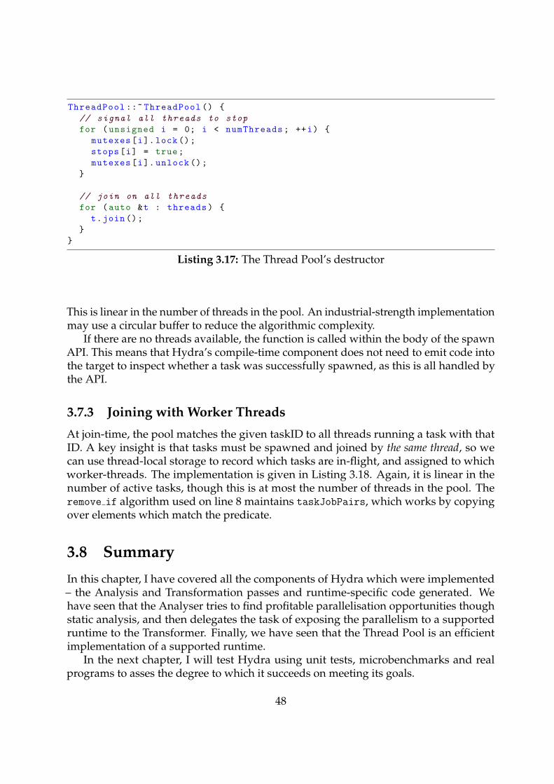
ThreadPool ::~ ThreadPool () {
// signal all threads to stop
for (unsigned i = 0; i < numThreads; ++i) {
mutexes[i].lock();
stops[i] = true;
mutexes[i]. unlock ();
}
// join on all threads
for (auto &t : threads) {
t.join();
}
}
Listing 3.17: The Thread Pool’s destructor
This is linear in the number of threads in the pool. An industrial-strength implementationmay use a circular buffer to reduce the algorithmic complexity.
If there are no threads available, the function is called within the body of the spawnAPI. This means that Hydra’s compile-time component does not need to emit code intothe target to inspect whether a task was successfully spawned, as this is all handled bythe API.
3.7.3 Joining with Worker Threads
At join-time, the pool matches the given taskID to all threads running a task with thatID. A key insight is that tasks must be spawned and joined by the same thread, so wecan use thread-local storage to record which tasks are in-flight, and assigned to whichworker-threads. The implementation is given in Listing 3.18. Again, it is linear in thenumber of active tasks, though this is at most the number of threads in the pool. Theremove if algorithm used on line 8 maintains taskJobPairs, which works by copyingover elements which match the predicate.
3.8 Summary
In this chapter, I have covered all the components of Hydra which were implemented– the Analysis and Transformation passes and runtime-specific code generated. Wehave seen that the Analyser tries to find profitable parallelisation opportunities thoughstatic analysis, and then delegates the task of exposing the parallelism to a supportedruntime to the Transformer. Finally, we have seen that the Thread Pool is an efficientimplementation of a supported runtime.
In the next chapter, I will test Hydra using unit tests, microbenchmarks and realprograms to asses the degree to which it succeeds on meeting its goals.
48
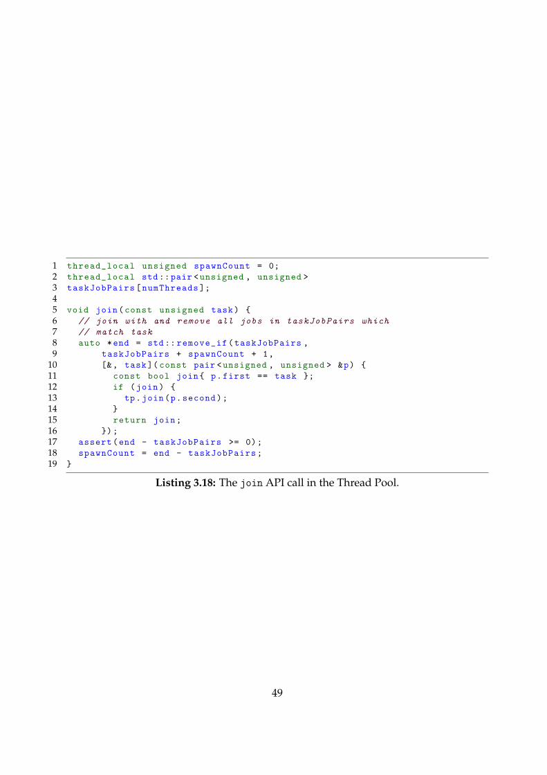
1 thread_local unsigned spawnCount = 0;
2 thread_local std::pair <unsigned , unsigned >
3 taskJobPairs[numThreads ];
45 void join(const unsigned task) {
6 // join with and remove all jobs in taskJobPairs which
7 // match task
8 auto *end = std:: remove_if(taskJobPairs ,
9 taskJobPairs + spawnCount + 1,
10 [&, task]( const pair <unsigned , unsigned > &p) {
11 const bool join{ p.first == task };
12 if (join) {
13 tp.join(p.second);
14 }
15 return join;
16 });
17 assert(end - taskJobPairs >= 0);
18 spawnCount = end - taskJobPairs;
19 }
Listing 3.18: The join API call in the Thread Pool.
49

50
Chapter 4
Evaluation
This chapter shows all that was done to establish that Hydra works as intended, butalso how well the function offloading performs in practice. As Hydra is a compilerextension, unit tests are of high importance due to low tolerance to incorrectness andnumerous corner cases. We will see how test cases were constructed (§4.2) and howthe runtimes were evaluated for efficiency (§4.3). Finally, I apply Hydra to a real-worldsimulation problem, demonstrating that it successfully speeds up the completion byauto-parallelising it (§4.4).
4.1 Overall Results
In the Requirements Analysis (§2.3), requirements were specified for each of the threecomponents of Hydra: the Analyser, Transformer and Thread Pool.
The Analyser is required to ‘determine which functions are fit for spawning and [. . . ]at which callsides of those functions offloading is profitable’. The Analyser was identifiedas being of maximal importance for a successful project, so its goals were met at thebeginning of the implementation, as described in §3.1–3.4. The result is a sequence ofoptimisation passes, which ultimately outputs which callsites should be offloaded, aswell as where to join with the offloaded call.
The Transformer is required to ‘communicate to a supported runtime that certain functioncalls [. . . ] should be offloaded.’. This was implemented after the Analyser, as described in§3.5 and §3.6. It is able to add the relevent API declarations into an IR module, and emitspawn and join API calls at the point of offload.
The Thread Pool is required to be a ‘supported runtime of the Analyser and Transformerwhich performs function offloading using an Eager Thread Pool design’. This was the last com-ponent of Hydra to be implemented, but it has nonetheless been effective, as describedin §3.7.
51
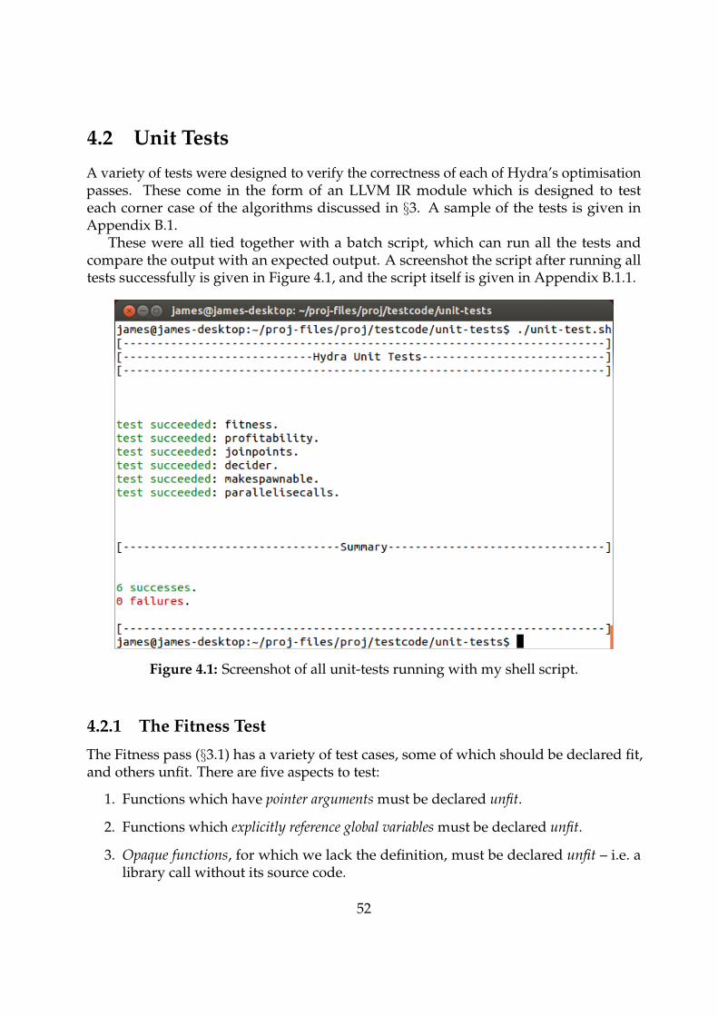
4.2 Unit Tests
A variety of tests were designed to verify the correctness of each of Hydra’s optimisationpasses. These come in the form of an LLVM IR module which is designed to testeach corner case of the algorithms discussed in §3. A sample of the tests is given inAppendix B.1.
These were all tied together with a batch script, which can run all the tests andcompare the output with an expected output. A screenshot the script after running alltests successfully is given in Figure 4.1, and the script itself is given in Appendix B.1.1.
Figure 4.1: Screenshot of all unit-tests running with my shell script.
4.2.1 The Fitness Test
The Fitness pass (§3.1) has a variety of test cases, some of which should be declared fit,and others unfit. There are five aspects to test:
1. Functions which have pointer arguments must be declared unfit.
2. Functions which explicitly reference global variables must be declared unfit.
3. Opaque functions, for which we lack the definition, must be declared unfit – i.e. alibrary call without its source code.
52
4. Functions which call unfit functions must be declared unfit.
5. All other functions must be declared fit.
These are tested using a module with five functions, one for each aspect. The FitnessTest module and expected output is given in Appendix B.1.2.
4.2.2 The Profitability Test
For Profitability, I needed to test that the pass correctly calculates the h3 heuristic pre-sented in §3.2.4. To do this, I designed some IR modules, and computed h3 for each byhand. Note that the value of h3 depends on the output from LLVM’s ScalarEvolution, soI needed to run the module through it to do the calculation.
In order to stress the corner cases of h3, I made a function with a loop, a functionwith recursion, a function with a loop and recursion, and functions which call cheap andexpensive functions.
4.2.3 The JoinPoints Test
To test JoinPoints, I designed two spawn points: one with the join inside the spawnblock, and one where there were joins in multiple blocks. Note that when testing on theKernel Threads runtime, both these examples should put the join in the spawn block,for reasons discussed in §3.3.2. For the Thread Pool runtime, we need to test that blockswith joins, blocks without joins, CFGs with loops, blocks with returns, and looping backaround to the spawn block all work as expected.
4.2.4 The Decider Test
The correctness of the Decider is quite sensitive to the correctness of Profitability andJoinPoints, so this test is written under the assumption that those work correctly.
There are two key pieces of functionality to test in the decider:
1. cost(caller) is being calculated correctly, using each of the three methods of combin-ing all the results (§3.4.3).
2. The Profitability Condition (Figure 2.3) is being applied correctly.
The first of these cannot be tested directly, since the Decider does not remembercost(caller) after its decision has been made. Hence, I adopted an indirect method to testthis: I designed examples where the choice of combination method should change thedecision made.
53
4.2.5 The MakeSpawnable Test
All we need to see here is that the MakeSpawnable pass is correctly synthesising spawn-able versions of functions, armed with the correct types and bitcasts. We also need tocheck that it does not synthesise spawnable versions of functions that are not going to beparallelised.
4.2.6 The ParalleliseCalls Test
ParalleliseCalls has a fair bit of functionality that needs to be tested, which is enumeratedbelow. The Module that was written tests all these features.
1. Name mangling is working correctly for the Itanium C++ ABI (§3.6.1).
2. Task IDs are being correctly generated for Thread Pool calls. Note that we have touse a constant seed for the generator to ensure that the test results are deterministic.
3. Appropriate bitcasts and allocas are being added at the spawn site.
4. The return value of parallelised calls is being handled properly.
4.3 Runtime Microbenchmarks
The Profitability Condition (Figure 2.3) has three quantities. Two of them are establishedthrough static analysis, and the third, cost(spawn), is found empirically. Here I will showhow this value was estimated for Hydra’s two supported runtimes.
It is important to understand the units of cost(spawn). Observing the ProfitabilityEquation tells us that it must have the same units as the other two quantities, which wereestimated using heuristics based on the number of IR Instructions in §3.2 and §3.4. Thus,the required units must also be number of IR instructions.
Since measuring IR instruction counts directly is difficult, I chose an indirect approach:I measured the time it took to execute a spawn followed immediately by a join, and thennormalised the time to that taken to execute a simple increment operation. An incrementrequires three IR instructions, and we can thus derive an approximation of the numberof IR instructions needed for a spawn/join from this measurement An example of thecode which generated one of the test results is given in Appendix B.2.
The results are given in Figure 4.2. We see that the Thread Pool outperforms Ker-nel Threads, managing to join in 10× fewer instructions.
The Thread Pool runtime tests were performed twice: once when the pool was empty(cost of a successful spawn and join), and once when the pool was at capacity (cost ofa failed spawn and benign join). The results are coloured green and red respectively.As predicted in §2.2.2, the cost of a failed spawn is low, usually no more than 10 IRinstructions, but this is perhaps not small enough to be ignored entirely, suggesting apossible refinement to the Analyser.
54
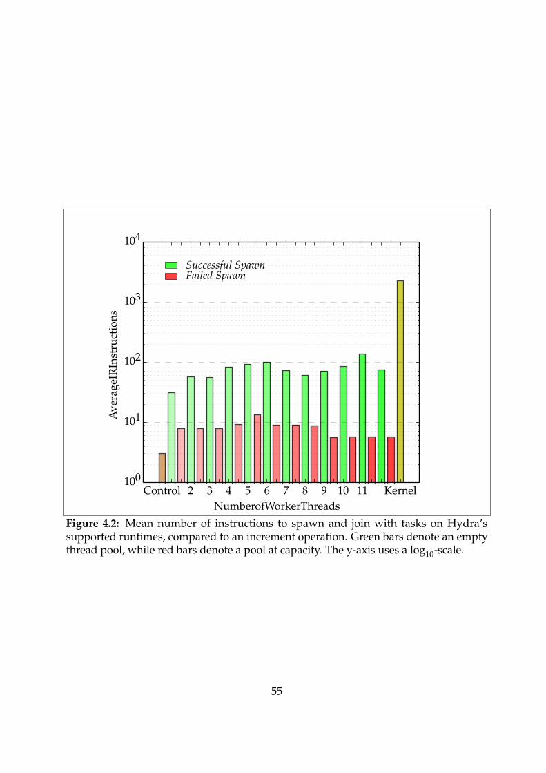
Control 2 3 4 5 6 7 8 9 10 11 KernelNumberofWorkerThreads
100
101
102
103
104
Ave
rage
IRIn
stru
ctio
ns
Successful SpawnFailed Spawn
Figure 4.2: Mean number of instructions to spawn and join with tasks on Hydra’ssupported runtimes, compared to an increment operation. Green bars denote an emptythread pool, while red bars denote a pool at capacity. The y-axis uses a log10-scale.
55
In addition, the Thread Pool runtime tests were repeated for pools with differentnumbers of worker threads, but the differences are relatively minor. As discussed in §3.7,spawn and join are linear-time operations, but the constant factor seems too small tomake a difference at 12 worker threads.
The tests produced quite a few anomalous results, probably due to a context switchoccurring in between the timer points. As far as the Analyser is concerned, these contextswitches would have occurred anyway, so are not interesting when making an offloaddecision. In addition, the first spawn is consistently slower than subsequent spawns.This is best explained by the first test having a cache miss, hinting at another possiblerefinement to the analysis.
4.4 Performance Testing
To test Hydra’s performance on a macroscopic level, I implemented a well-knownalgorithm which has a lot of parallelism available for extraction – n-body simulation.1
However, my implementation is serial, i.e. it does not have any built-in parallelismwhatsoever. It is up to Hydra to find and extract the parallelism.
N-body simulation is a numerical approach to the n-body problem: solving thetrajectories of n gravitational bodies.2 It is proven that, for n > 2, the n-body problemhas no analytical solution, which makes simulation very popular.
My implementation of the algorithm, given in §B.3, iterates over each body, updatingits velocity and position. Computing this update is quite costly, since we must loop overeach other body in the scene and compute the inverse squared distance. Hence, Hydra isable to offload the update function.3
The code was compiled using Clang 3.4 targeting the x86-64 architecture. I decidedto use optimisation level ‘O1’ in order for the results to be reflective of my project’scontribution to performance rather than Clang’s optimiser. However, I felt that O0
performance was unrepresentative.4
To expose parallelism from within the main loop, I used a technique called loopunrolling, where a loop is transformed such that the body of the new loop executesmultiple iterations of the old loop. LLVM implements automatic loop unrolling and,with additional engineering effort, the project could hook into this for automatic loopparallelism extraction.
1Due to the fragile nature of n-body simulation, it also served as a good correctness test for the runtimes,since any errors would effect the observable output.
2http://bit.ly/1iGtPzS3I do need to make a special case of these functions, since Fitness is rejecting them due to pointer
arguments (§3.1). This is safe to do, since they do not modify the pointee (§2.1.2). With additionalengineering work, I am confident that Fitness will be able to identify such use automatically.
4The Thread Pool itself was compiled at O3, since the Analyser’s cost model relies on a highly optimisedThread Pool.
56
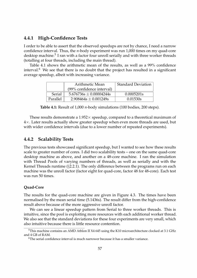
4.4.1 High-Confidence Tests
I order to be able to assert that the observed speedups are not by chance, I need a narrowconfidence interval. Thus, the n-body experiment was run 1,000 times on my quad-coredesktop machine.5 I ran with a factor four unroll serially and with three worker threads(totalling at four threads, including the main thread).
Table 4.1 shows the arithmetic mean of the results, as well as a 99% confidenceinterval.6 We see that there is no doubt that the project has resulted in a significantaverage speedup, albeit with increasing variance.
Arithmetic Mean(99% confidence interval)
Standard Deviation
Serial 5.676736s± 0.00004244s 0.0005201sParallel 2.908464s± 0.001249s 0.01530s
Table 4.1: Result of 1,000 n-body simulations (100 bodies, 200 steps).
These results demonstrate a 1.952× speedup, compared to a theoretical maximum of4×. Later results actually show greater speedup when even more threads are used, butwith wider confidence intervals (due to a lower number of repeated experiments).
4.4.2 Scalability Tests
The previous tests showcased significant speedup, but I wanted to see how these resultsscale to greater number of cores. I did two scalability tests – one on the same quad-coredesktop machine as above, and another on a 48-core machine. I ran the simulationwith Thread Pools of varying numbers of threads, as well as serially and with theKernel Threads runtime (§2.2.1). The only difference between the programs run on eachmachine was the unroll factor (factor eight for quad-core, factor 48 for 48-core). Each testwas run 50 times.
Quad-Core
The results for the quad-core machine are given in Figure 4.3. The times have beennormalised by the mean serial time (5.1436s). The result differ from the high-confidenceresult above because of the more aggressive unroll factor.
We can see a linear speedup pattern from Serial to three worker threads. This isintuitive, since the pool is exploiting more resources with each additional worker thread.We also see that the standard deviations for these four experiments are very small, whichalso intuitive because there is little resource contention.
5This machine contains an AMD Athlon II X4 645 using the K10 microarchitecture clocked at 3.1 GHzand 4 GB of RAM.
6The serial confidence interval is much narrower because it has a smaller variance.
57
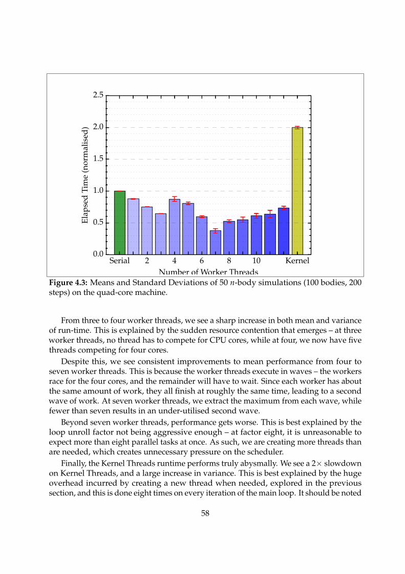
Serial 2 4 6 8 10 KernelNumber of Worker Threads
0.0
0.5
1.0
1.5
2.0
2.5El
apse
dTi
me
(nor
mal
ised
)
Figure 4.3: Means and Standard Deviations of 50 n-body simulations (100 bodies, 200steps) on the quad-core machine.
From three to four worker threads, we see a sharp increase in both mean and varianceof run-time. This is explained by the sudden resource contention that emerges – at threeworker threads, no thread has to compete for CPU cores, while at four, we now have fivethreads competing for four cores.
Despite this, we see consistent improvements to mean performance from four toseven worker threads. This is because the worker threads execute in waves – the workersrace for the four cores, and the remainder will have to wait. Since each worker has aboutthe same amount of work, they all finish at roughly the same time, leading to a secondwave of work. At seven worker threads, we extract the maximum from each wave, whilefewer than seven results in an under-utilised second wave.
Beyond seven worker threads, performance gets worse. This is best explained by theloop unroll factor not being aggressive enough – at factor eight, it is unreasonable toexpect more than eight parallel tasks at once. As such, we are creating more threads thanare needed, which creates unnecessary pressure on the scheduler.
Finally, the Kernel Threads runtime performs truly abysmally. We see a 2× slowdownon Kernel Threads, and a large increase in variance. This is best explained by the hugeoverhead incurred by creating a new thread when needed, explored in the previoussection, and this is done eight times on every iteration of the main loop. It should be noted
58
that I had to reduce what the Analyser believed to be the overheads of Kernel Threads inorder to make it parallelise the code at all, since the actual overheads cannot balance theProfitability Condition (Figure 2.3).
48-Core
The results of the 48-core machine7 are given in Figure 4.4. These have been normalised,just as above, by the mean serial time (7.74786s). Note that serial performance on is worsethan that of the quad-core machine above due to the difference in base clock frequency(2.6 GHz vs 3.1 GHz).
We observe linear speedup, peaking with 6.33× speedup at about 47 worker threads.Past 47 workers, performance degrades as we add pressure to the scheduler for no realimprovement in extracted parallelism. This linear speedup is a pleasing result, andnegates the concerns of synchronisation costs diminishing the gains.
We do observe an almost periodic rise and fall in variance as the number of workerthreads increases. This is best explained by the machine’s Non-Uniform Memory Access(NUMA) memory design [13]. The machine’s 128 GB of RAM is divided into fourmemory controllers attached to four sockets, where each socket contains 12 of the 48cores. When a core attempts to access memory which does not reside in its socket, it mustmake a remote access request to pull in the data from the other socket. The result of thisis that cores on the same socket share memory more efficiently than cores on differentsockets.
Once the data has been fetched from a remote socket, it will be cached in the currentsocket’s cache hierarchy. This means that, in our experiment, when lots of threads areallocated to the same socket, fewer remote accesses are required.8 As the Linux scheduleris under a lot of pressure to schedule threads quickly, it will usually not consider NUMAcache affinity when scheduling threads onto cores. As a result, we experienced increasedvariance of performance due to the degree of chance in receiving a good scheduling. Thisalso explains the pseudo-periodicity of variance.9
To my delight, even the Kernel Threads runtime performed quite respectably. Ibelieve this because the Linux kernel itself is more able to create threads in parallel onthe 48-core machine compared to my own desktop.
7The machine contains an AMD Opteron 6344 using the Abu Dhabi microarchitecture clocked at2.6 GHz base, with 2.9–3.2 GHz turbo, and 128 GB of RAM. For more details, see http://bit.ly/1oFV9z6.
8When one core pulls data into the socket’s cache, the other cores experience cache hits when theyrequest the same data for reading.
9Remote accesses rise with number of threads, but plateau once all four sockets are used. As number ofthreads increases further, we experience more cache hits due to neighbouring cores pulling shared datainto the socket’s cache.
59
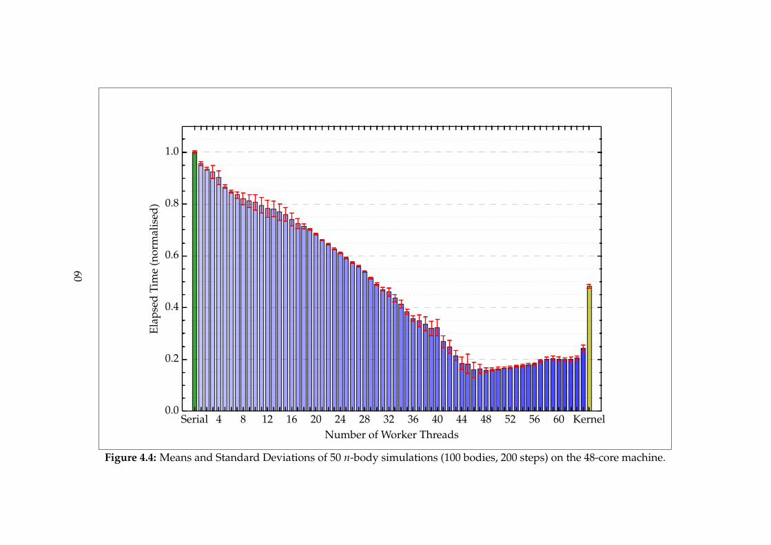
Serial 4 8 12 16 20 24 28 32 36 40 44 48 52 56 60 KernelNumber of Worker Threads
0.0
0.2
0.4
0.6
0.8
1.0El
apse
dTi
me
(nor
mal
ised
)
Figure 4.4: Means and Standard Deviations of 50 n-body simulations (100 bodies, 200 steps) on the 48-core machine.
60
Chapter 5
Conclusions
In this dissertation, I have explained all the preparation, implementation and evaluationI undertook in the development of Hydra.
When I decided to undertake this project, I desired to learn more about compilation,particularly optimising compilation, and parallelisation. Looking back, the project hascertainly delivered: I had the opportunity to explore and experiment with leadingcompiler technology, and found myself inevitably learning a lot about related fields byosmosis. While Hydra is not a research project by nature, the difficult problems I facedhave certainly increased my appetite for research in this field.
5.1 Results
As discussed in §4.1, Hydra has met all the requirements laid out in the RequirementsAnalysis (§2.3), which has been verified through careful testing (§4.2).
Hydra has even gained a few unplanned extensions along the way. In particular,many of the improvements to the Profitability (§3.2), JoinPoints (§3.3) and the Decider(§3.4) analysis passes were ultimately included, some of which were not conceived untila fair way into Hydra’s implementation. In addition, the Thread Pool itself (§3.7), a majorcontributor to Hydra and its success, was a project extension. While Hydra’s Thread Poolruntime may be a little primitive compared to some its industrial counterparts, I findthere is elegance in its simplicity and portability which, when coupled with its impressiveperformance (§4.4), is very pleasing.
In addition to Hydra attaining its goals, I find that I have also progressed significantlyas a direct result of this project. As well as further exposing me to an endlessly fascinatingfield, the project has given me many practical skills that I am sure will be transferred tomy future career. I have gained greater appreciation of the discipline and effort requiredto build a sizeable piece of software, on top of the knowledge of many new tools, andeven advancing my skills in technical writing.
61
5.2 Lessons Learnt
Perhaps it was naıve of me to suspect that I could successfully create a fully automaticfunction paralleliser when little of that nature currently exists. In spite of this, I havemanaged to create something which is completely successful in what it sets out to achieve,and even though I have learnt of the perils of underestimating the difficulty of a problemat the outset, maybe it was this naıvety that has made Hydra as successful as it is.
5.3 Future Work
While I managed to add more extensions into Hydra than I could have thought possiblewhen proposing the project, the complexity of the problems faced mean that there isinevitably more that could have been done. As such, I am planning to ultimately includethe features given below in a future iteration of Hydra. I am also planning to release thesource code for others to download and peruse.
• As Hydra’s implementation neared its completion, the value of Profile GuidedOptimisation (PGO) became clear to me. The static analysis techniques used inHydra’s Analyser will always have limitations. In particular, it is usually impossibleto reason about the behaviour of program inputs in an unsupervised manner. PGOempowers us with this knowledge, which is immensely valuable. In my mind,however, it is clear that PGO is not a replacement for static analysis – in fact, I findthe two to be complementary.
• Support for exceptions – first within in the program, but not offloaded functions,and then also in offloaded functions.
• Allowing functions with pointer arguments, in some limited cases where the analysisis tractable, e.g. read-only functions.
62
Bibliography
[1] David W. Wall. Limits of Instruction-Level Parallelism Palo Alto, CA, USA, 1992.
[2] Robert D. Blumofe, Christopher F. Joerg, Bradley C. Kuszmaul, Charles E. Leiserson,Keith H. Randall, and Yuli Zhou. Cilk: An Efficient Multithreaded Runtime System MITLaboratory for Computer Science, 1995.
[3] Dagum, L.; Menon, R. OpenMP: an industry standard API for shared-memory program-ming. Computational Science & Engineering, IEEE, 1998.
[4] Simon Campanoni, Timothy Jones, Glenn Holloway, Gu-Yeon Wei and David Brooks.The HELIX Project: Overview and Directions Harvard University, Cambridge, USAand University of Cambridge, Cambridge, UK, 2012.
[5] Dorit Naishlos. Autovectorisation in GCC. GCC Developers’ Summit, 2004.
[6] Tobias Grosser, Hongbin Zheng, Raghes Aloor, Andreas Simburger, ArminGroßlinger and Louis-Noel Pouchet. Polly – Polyhedral optimization in LLVM. Univer-sitat Passau, Sun Yat-Sen University, Indian Institue of Technology and Ohio StateUniversity, 2011.
[7] Derek G. Murray, Malte Schwarzkopf, Christopher Smowton, Steven Smtih, AnilMadhavapeddy and Steven Hand. CIEL: a universal execution engine for distributeddataflow computing. University of Cambridge Computer Laboratory, 2010.
[8] Chris Lattner and Vikram Adve. LLVM: A Compilation Framework for Lifelong ProgramAnalysis & Transformation. Palo Alto, CA, USA, 2004.
[9] H. Hinnant, L. Crowl, B. Dawes, A. Williams, J. Garland, et al. Multi-threading Libraryfor Standard C++ (Revision 1). ISO/IEC, 2008.
[10] ISO/IEC 9899. TC2 Committee Draft. ISO. 2005. pp. 108–112.
[11] Dijkstra, E. W. A note on two problems in the connexion with graphs. NumerischeMathematik, 1959.
[12] Makoto Matsumoto and Takuji Nishimura. Mersenne Twister: A 623-dimensionallyequidistributed uniform pseudorandom number generator. Keio University/Max-Planck-Institut fur Mathematik, 1998.
63

[13] Nakul Manchanda and Karan Anand. Non-Uniform Memory Access (NUMA). NewYork University, 2010.
[14] Jeffrey Dean and Sanjay Ghemawat. MapReduce: simplified data processing on largeclusters. ACM, New York, NY, USA, 2008.
64
Appendix A
C++11, the 2011 standard for C++
When I first learnt C++, I was vaguely aware of a new ‘C++0x/11’ standard. However,at the time, compiler support was minimal, so I did not end up learning it. However,just before I started writing the proposal for Hydra, two open-source compilers, Clangand GCC, became C++11 compliant. This motivated me to start reading about the newstandard and shortly after, I made the decision to use these extensions in this project.Below is a list of new language features used in Hydra. In addition, several of the newlibraries were used, given in §2.6.2.
• Move Semantics.
• Generalised constant expressions with constexpr.
• Uniform initialisation syntax and initialiser lists.
• Type inference with auto.
• Range-based for loops.
• Lambda expressions.
• Null pointer constant with nullptr.
• Strongly typed enumerations with enum class.
• Thread-local storage with thread local.
65

66
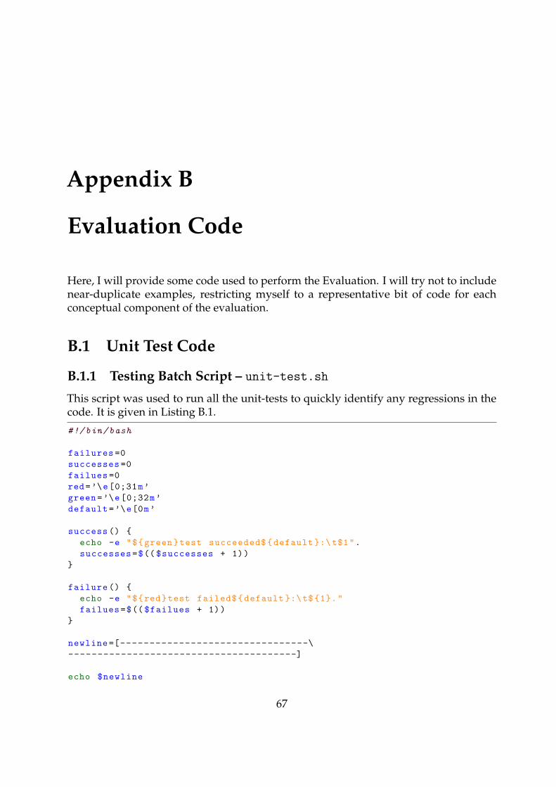
Appendix B
Evaluation Code
Here, I will provide some code used to perform the Evaluation. I will try not to includenear-duplicate examples, restricting myself to a representative bit of code for eachconceptual component of the evaluation.
B.1 Unit Test Code
B.1.1 Testing Batch Script – unit-test.sh
This script was used to run all the unit-tests to quickly identify any regressions in thecode. It is given in Listing B.1.
#!/bin/bash
failures =0
successes =0
failues =0
red=’\e[0;31m’
green=’\e[0;32m’
default=’\e[0m’
success () {
echo -e "${green}test succeeded${default }:\ t$1".
successes=$(( $successes + 1))
}
failure () {
echo -e "${red}test failed${default }:\t${1}."
failues=$(( $failues + 1))
}
newline=[--------------------------------\
---------------------------------------]
echo $newline
67
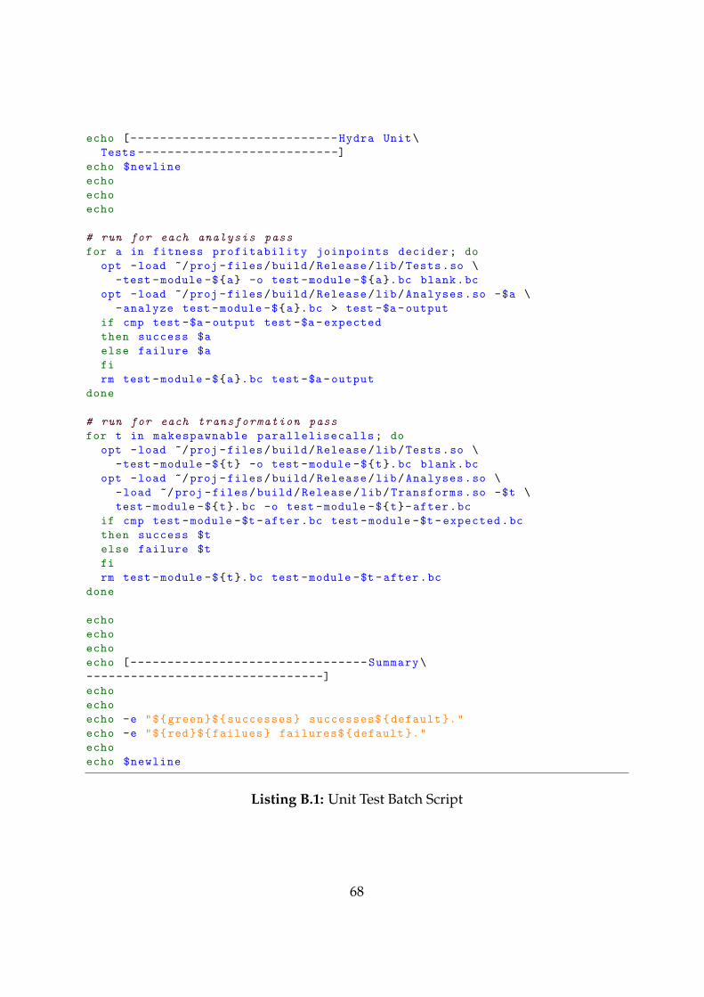
echo [----------------------------Hydra Unit\
Tests ---------------------------]
echo $newline
echo
echo
echo
# run for each analysis pass
for a in fitness profitability joinpoints decider; do
opt -load ~/proj -files/build/Release/lib/Tests.so \
-test -module -${a} -o test -module -${a}.bc blank.bc
opt -load ~/proj -files/build/Release/lib/Analyses.so -$a \
-analyze test -module -${a}.bc > test -$a -output
if cmp test -$a -output test -$a -expected
then success $a
else failure $a
fi
rm test -module -${a}.bc test -$a -output
done
# run for each transformation pass
for t in makespawnable parallelisecalls; do
opt -load ~/proj -files/build/Release/lib/Tests.so \
-test -module -${t} -o test -module -${t}.bc blank.bc
opt -load ~/proj -files/build/Release/lib/Analyses.so \
-load ~/proj -files/build/Release/lib/Transforms.so -$t \
test -module -${t}.bc -o test -module -${t}-after.bc
if cmp test -module -$t -after.bc test -module -$t -expected.bc
then success $t
else failure $t
fi
rm test -module -${t}.bc test -module -$t -after.bc
done
echo
echo
echo
echo [--------------------------------Summary\
--------------------------------]
echo
echo
echo -e "${green}${successes} successes${default }."
echo -e "${red}${failues} failures${default }."
echo
echo $newline
Listing B.1: Unit Test Batch Script
68
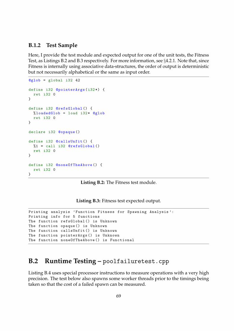
B.1.2 Test Sample
Here, I provide the test module and expected output for one of the unit tests, the FitnessTest, as Listings B.2 and B.3 respectively. For more information, see §4.2.1. Note that, sinceFitness is internally using associative data-structures, the order of output is deterministicbut not necessarily alphabetical or the same as input order.
@glob = global i32 42
define i32 @pointerArgs(i32*) {
ret i32 0
}
define i32 @refsGlobal () {
%loadedGlob = load i32* @glob
ret i32 0
}
declare i32 @opaque ()
define i32 @callsUnfit () {
%1 = call i32 @refsGlobal ()
ret i32 0
}
define i32 @noneOfTheAbove () {
ret i32 0
}
Listing B.2: The Fitness test module.
Listing B.3: Fitness test expected output.
Printing analysis ’Function Fitness for Spawning Analysis ’:
Printing info for 5 functions
The function refsGlobal () is Unknown
The function opaque () is Unknown
The function callsUnfit () is Unknown
The function pointerArgs () is Unknown
The function noneOfTheAbove () is Functional
B.2 Runtime Testing – poolfailuretest.cpp
Listing B.4 uses special processor instructions to measure operations with a very highprecision. The test below also spawns some worker threads prior to the timings beingtaken so that the cost of a failed spawn can be measured.
69
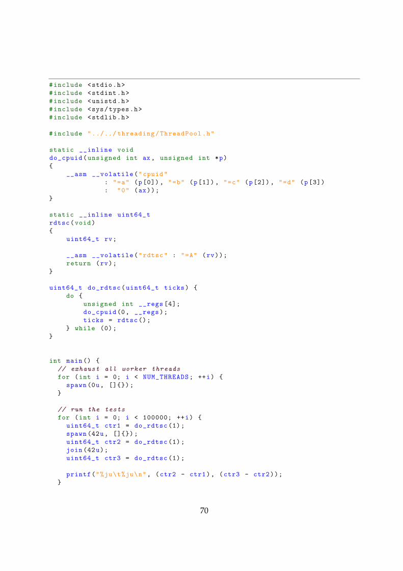
#include <stdio.h>
#include <stdint.h>
#include <unistd.h>
#include <sys/types.h>
#include <stdlib.h>
#include "../../ threading/ThreadPool.h"
static __inline void
do_cpuid(unsigned int ax, unsigned int *p)
{
__asm __volatile("cpuid"
: "=a" (p[0]), "=b" (p[1]), "=c" (p[2]), "=d" (p[3])
: "0" (ax));
}
static __inline uint64_t
rdtsc(void)
{
uint64_t rv;
__asm __volatile("rdtsc" : "=A" (rv));
return (rv);
}
uint64_t do_rdtsc(uint64_t ticks) {
do {
unsigned int __regs [4];
do_cpuid(0, __regs);
ticks = rdtsc ();
} while (0);
}
int main() {
// exhaust all worker threads
for (int i = 0; i < NUM_THREADS; ++i) {
spawn(0u, []{});
}
// run the tests
for (int i = 0; i < 100000; ++i) {
uint64_t ctr1 = do_rdtsc (1);
spawn (42u, []{});
uint64_t ctr2 = do_rdtsc (1);
join (42u);
uint64_t ctr3 = do_rdtsc (1);
printf("%ju\t%ju\n", (ctr2 - ctr1), (ctr3 - ctr2));
}
70
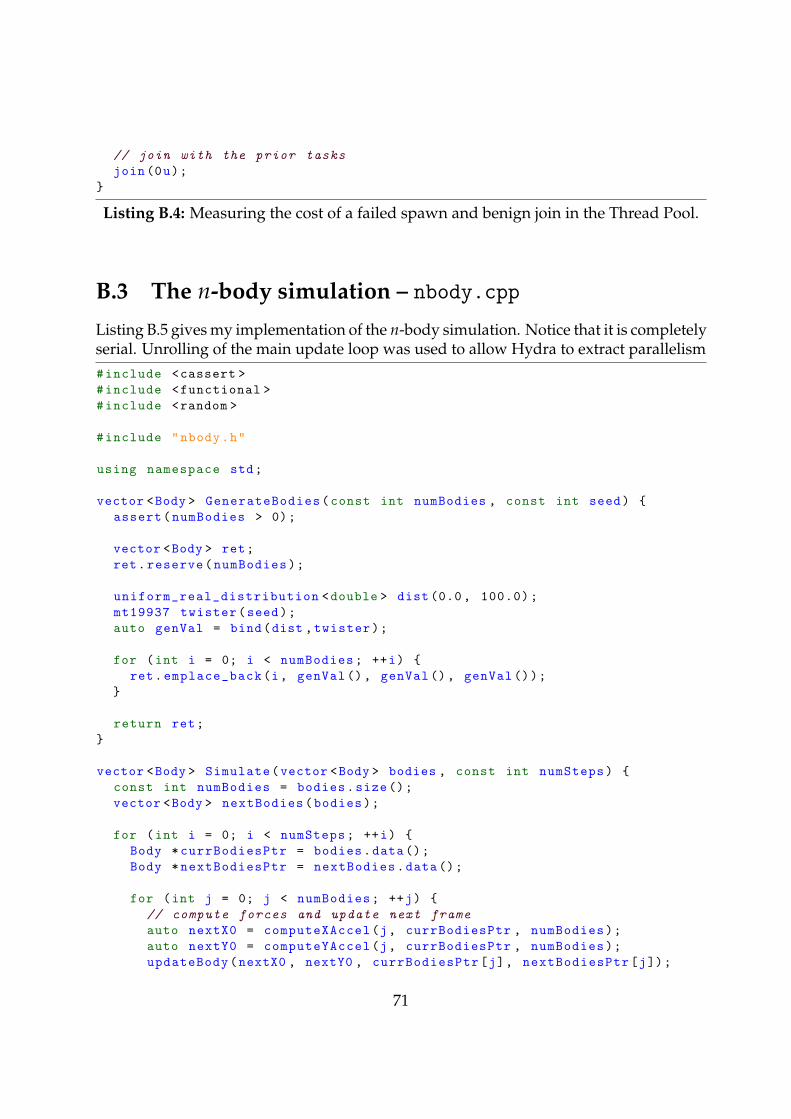
// join with the prior tasks
join(0u);
}
Listing B.4: Measuring the cost of a failed spawn and benign join in the Thread Pool.
B.3 The n-body simulation – nbody.cpp
Listing B.5 gives my implementation of the n-body simulation. Notice that it is completelyserial. Unrolling of the main update loop was used to allow Hydra to extract parallelism#include <cassert >
#include <functional >
#include <random >
#include "nbody.h"
using namespace std;
vector <Body > GenerateBodies(const int numBodies , const int seed) {
assert(numBodies > 0);
vector <Body > ret;
ret.reserve(numBodies);
uniform_real_distribution <double > dist (0.0, 100.0);
mt19937 twister(seed);
auto genVal = bind(dist ,twister);
for (int i = 0; i < numBodies; ++i) {
ret.emplace_back(i, genVal (), genVal (), genVal ());
}
return ret;
}
vector <Body > Simulate(vector <Body > bodies , const int numSteps) {
const int numBodies = bodies.size();
vector <Body > nextBodies(bodies);
for (int i = 0; i < numSteps; ++i) {
Body *currBodiesPtr = bodies.data();
Body *nextBodiesPtr = nextBodies.data();
for (int j = 0; j < numBodies; ++j) {
// compute forces and update next frame
auto nextX0 = computeXAccel(j, currBodiesPtr , numBodies);
auto nextY0 = computeYAccel(j, currBodiesPtr , numBodies);
updateBody(nextX0 , nextY0 , currBodiesPtr[j], nextBodiesPtr[j]);
71
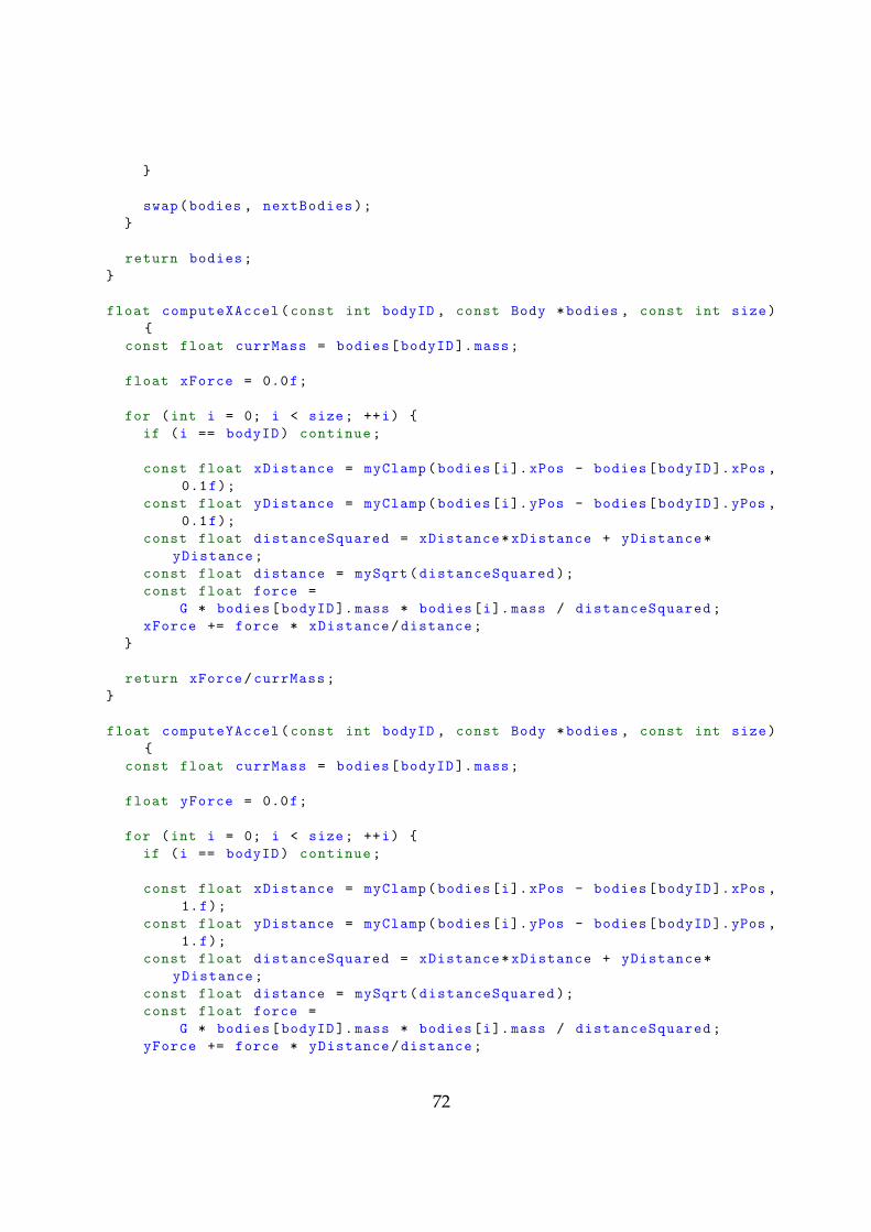
}
swap(bodies , nextBodies);
}
return bodies;
}
float computeXAccel(const int bodyID , const Body *bodies , const int size)
{
const float currMass = bodies[bodyID ].mass;
float xForce = 0.0f;
for (int i = 0; i < size; ++i) {
if (i == bodyID) continue;
const float xDistance = myClamp(bodies[i].xPos - bodies[bodyID ].xPos ,
0.1f);
const float yDistance = myClamp(bodies[i].yPos - bodies[bodyID ].yPos ,
0.1f);
const float distanceSquared = xDistance*xDistance + yDistance*
yDistance;
const float distance = mySqrt(distanceSquared);
const float force =
G * bodies[bodyID ].mass * bodies[i].mass / distanceSquared;
xForce += force * xDistance/distance;
}
return xForce/currMass;
}
float computeYAccel(const int bodyID , const Body *bodies , const int size)
{
const float currMass = bodies[bodyID ].mass;
float yForce = 0.0f;
for (int i = 0; i < size; ++i) {
if (i == bodyID) continue;
const float xDistance = myClamp(bodies[i].xPos - bodies[bodyID ].xPos ,
1.f);
const float yDistance = myClamp(bodies[i].yPos - bodies[bodyID ].yPos ,
1.f);
const float distanceSquared = xDistance*xDistance + yDistance*
yDistance;
const float distance = mySqrt(distanceSquared);
const float force =
G * bodies[bodyID ].mass * bodies[i].mass / distanceSquared;
yForce += force * yDistance/distance;
72
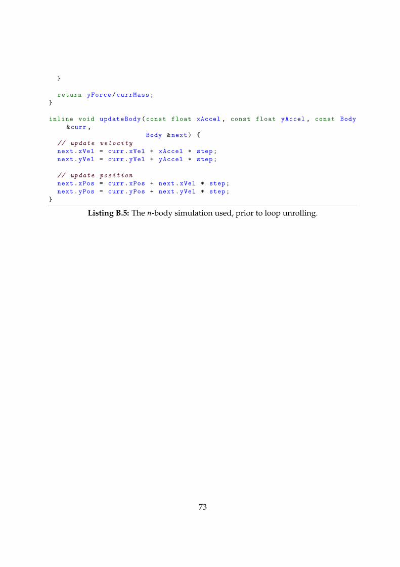
}
return yForce/currMass;
}
inline void updateBody(const float xAccel , const float yAccel , const Body
&curr ,
Body &next) {
// update velocity
next.xVel = curr.xVel + xAccel * step;
next.yVel = curr.yVel + yAccel * step;
// update position
next.xPos = curr.xPos + next.xVel * step;
next.yPos = curr.yPos + next.yVel * step;
}
Listing B.5: The n-body simulation used, prior to loop unrolling.
73

74
Appendix C
Project Proposal
Automatic Parallelism Across Multiple Threadsand More Using LLVMPart II Project Proposal
James Chickenjmc223
25th October 2013
C.1 Introduction and Description of the Work
Concurrent and distributed systems have become a ubiquitous part of the moderncomputing landscape. Clock speeds have ceased following Moore’s Law for some timenow, plateauing at around 3 GHz. As a result, we no longer live in a world where wecan write simple serial software and expect it to run twice as fast every couple of years.The path to faster software is clear: exploit more parallelism.
This is, of course, far from a new revelation: programmers have been writing parallelcode for decades. However, in that time, we have discovered that writing parallel code isfar from simple – many subtle bugs that are difficult to find creep into and thrive in ourparallel code, only rearing their ugly heads at the most inconvenient of times. Even if wecan manage to write correct parallel code, there is still no guarantee that it will actually
75
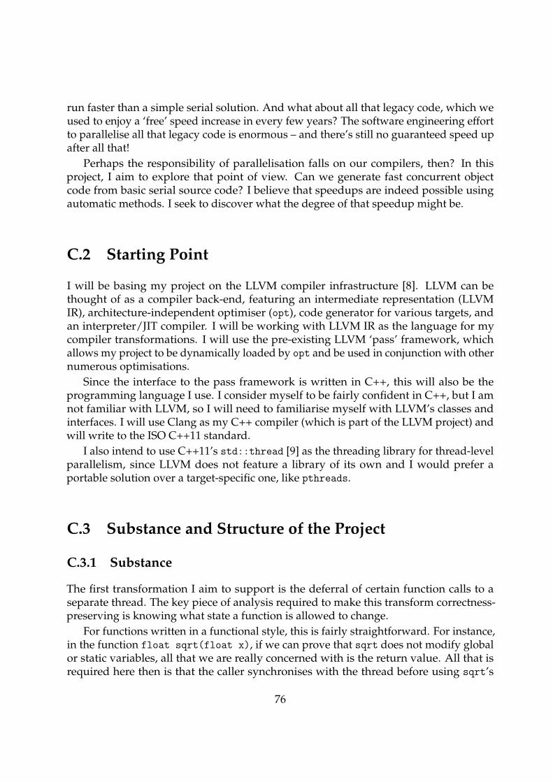
run faster than a simple serial solution. And what about all that legacy code, which weused to enjoy a ‘free’ speed increase in every few years? The software engineering effortto parallelise all that legacy code is enormous – and there’s still no guaranteed speed upafter all that!
Perhaps the responsibility of parallelisation falls on our compilers, then? In thisproject, I aim to explore that point of view. Can we generate fast concurrent objectcode from basic serial source code? I believe that speedups are indeed possible usingautomatic methods. I seek to discover what the degree of that speedup might be.
C.2 Starting Point
I will be basing my project on the LLVM compiler infrastructure [8]. LLVM can bethought of as a compiler back-end, featuring an intermediate representation (LLVMIR), architecture-independent optimiser (opt), code generator for various targets, andan interpreter/JIT compiler. I will be working with LLVM IR as the language for mycompiler transformations. I will use the pre-existing LLVM ‘pass’ framework, whichallows my project to be dynamically loaded by opt and be used in conjunction with othernumerous optimisations.
Since the interface to the pass framework is written in C++, this will also be theprogramming language I use. I consider myself to be fairly confident in C++, but I amnot familiar with LLVM, so I will need to familiarise myself with LLVM’s classes andinterfaces. I will use Clang as my C++ compiler (which is part of the LLVM project) andwill write to the ISO C++11 standard.
I also intend to use C++11’s std::thread [9] as the threading library for thread-levelparallelism, since LLVM does not feature a library of its own and I would prefer aportable solution over a target-specific one, like pthreads.
C.3 Substance and Structure of the Project
C.3.1 Substance
The first transformation I aim to support is the deferral of certain function calls to aseparate thread. The key piece of analysis required to make this transform correctness-preserving is knowing what state a function is allowed to change.
For functions written in a functional style, this is fairly straightforward. For instance,in the function float sqrt(float x), if we can prove that sqrt does not modify globalor static variables, all that we are really concerned with is the return value. All that isrequired here then is that the caller synchronises with the thread before using sqrt’s
76
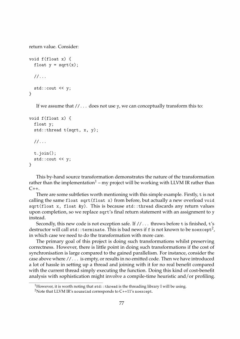
return value. Consider:
void f(float x) {
float y = sqrt(x);
//...
std::cout << y;
}
If we assume that //... does not use y, we can conceptually transform this to:
void f(float x) {
float y;
std::thread t(sqrt, x, y);
//...
t.join();
std::cout << y;
}
This by-hand source transformation demonstrates the nature of the transformationrather than the implementation1 – my project will be working with LLVM IR rather thanC++.
There are some subtleties worth mentioning with this simple example. Firstly, t is notcalling the same float sqrt(float x) from before, but actually a new overload void
sqrt(float x, float &y). This is because std::thread discards any return valuesupon completion, so we replace sqrt’s final return statement with an assignment to y
instead.Secondly, this new code is not exception safe. If //... throws before t is finished, t’s
destructor will call std::terminate. This is bad news if f is not known to be noexcept2,in which case we need to do the transformation with more care.
The primary goal of this project is doing such transformations whilst preservingcorrectness. However, there is little point in doing such transformations if the cost ofsynchronisation is large compared to the gained parallelism. For instance, consider thecase above where //... is empty, or results in no emitted code. Then we have introduceda lot of hassle in setting up a thread and joining with it for no real benefit comparedwith the current thread simply executing the function. Doing this kind of cost-benefitanalysis with sophistication might involve a compile-time heuristic and/or profiling.
1However, it is worth noting that std::thread is the threading library I will be using.2Note that LLVM IR’s nounwind corresponds to C++11’s noexcept.
77
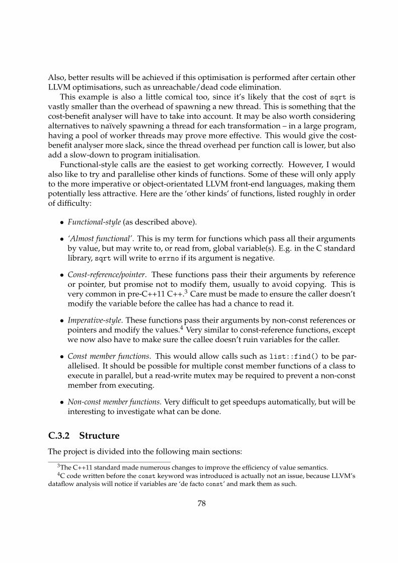
Also, better results will be achieved if this optimisation is performed after certain otherLLVM optimisations, such as unreachable/dead code elimination.
This example is also a little comical too, since it’s likely that the cost of sqrt isvastly smaller than the overhead of spawning a new thread. This is something that thecost-benefit analyser will have to take into account. It may be also worth consideringalternatives to naıvely spawning a thread for each transformation – in a large program,having a pool of worker threads may prove more effective. This would give the cost-benefit analyser more slack, since the thread overhead per function call is lower, but alsoadd a slow-down to program initialisation.
Functional-style calls are the easiest to get working correctly. However, I wouldalso like to try and parallelise other kinds of functions. Some of these will only applyto the more imperative or object-orientated LLVM front-end languages, making thempotentially less attractive. Here are the ‘other kinds’ of functions, listed roughly in orderof difficulty:
• Functional-style (as described above).
• ‘Almost functional’. This is my term for functions which pass all their argumentsby value, but may write to, or read from, global variable(s). E.g. in the C standardlibrary, sqrt will write to errno if its argument is negative.
• Const-reference/pointer. These functions pass their their arguments by referenceor pointer, but promise not to modify them, usually to avoid copying. This isvery common in pre-C++11 C++.3 Care must be made to ensure the caller doesn’tmodify the variable before the callee has had a chance to read it.
• Imperative-style. These functions pass their arguments by non-const references orpointers and modify the values.4 Very similar to const-reference functions, exceptwe now also have to make sure the callee doesn’t ruin variables for the caller.
• Const member functions. This would allow calls such as list::find() to be par-allelised. It should be possible for multiple const member functions of a class toexecute in parallel, but a read-write mutex may be required to prevent a non-constmember from executing.
• Non-const member functions. Very difficult to get speedups automatically, but will beinteresting to investigate what can be done.
C.3.2 Structure
The project is divided into the following main sections:
3The C++11 standard made numerous changes to improve the efficiency of value semantics.4C code written before the const keyword was introduced is actually not an issue, because LLVM’s
dataflow analysis will notice if variables are ‘de facto const’ and mark them as such.
78
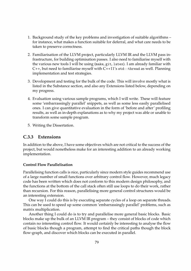
1. Background study of the key problems and investigation of suitable algorithms –for instance, what makes a function suitable for deferral, and what care needs to betaken to preserve correctness.
2. Familiarisation of the LLVM project, particularly LLVM IR and the LLVM pass in-frastructure, for building optimisation passes. I also need to familiarise myself withthe various new tools I will be using (make, git, latex). I am already familiar withC++, but need to familiarise myself with C++11’s std::thread as well. Planningimplementation and test strategies.
3. Development and testing for the bulk of the code. This will involve mostly what islisted in the Substance section, and also any Extensions listed below, depending onmy progress.
4. Evaluation using various sample programs, which I will write. These will featuresome ‘embarrassingly parallel’ snippets, as well as some less easily parallelisedones. I can give quantitative evaluation in the form of ‘before and after’ profilingresults, as well as in-depth explanations as to why my project was able or unable totransform some sample program.
5. Writing the Dissertation.
C.3.3 Extensions
In addition to the above, I have some objectives which are not critical to the success of theproject, but would nonetheless make for an interesting addition to an already workingimplementation.
Control Flow Parallelisation
Parallelising function calls is nice, particularly since modern style guides recommend useof a large number of small functions over arbitrary control flow. However, much legacycode has been written which does not conform to this modern design philosophy, andthe functions at the bottom of the call stack often still use loops to do their work, ratherthan recursion. For this reason, parallelising more general control structures would bean interesting extension.
One way I could do this is by executing separate cycles of a loop on separate threads.This can be used to speed up some common ‘embarrassingly parallel’ problems, such asmatrix multiplication.
Another thing I could do is to try and parallelise more general basic blocks. Basicblocks make up the bulk of an LLVM IR program – they consist of blocks of code whichcontain no interesting control flow. It would certainly be interesting to analyse the flowof basic blocks though a program, attempt to find the critical paths though the blockflow-graph, and discover which blocks can be executed in parallel.
79

Distributed Systems Parallelism
In the code written in my example above, one might notice how we generated codewhich executed the function on an std::thread. If this transformation was written in asufficiently general manner, it should be possible to instead generate code which can beexecuted on a remote machine in a distributed system. The code could be generated torun on a MapReduce system [14], for instance. However, MapReduce is not the mostnatural choice, since it takes JVM code as input. While it is possible to convert LLVM IRinto JVM, this does not fix the problem of library code, which is likely to be linked inobject form. A better option might be to use CIEL [7], a Cambridge project which canwork with a binary.
This does present some interesting problems, though. I would now have the option ofrunning a parallelised piece of code on a different thread locally, or remotely on anothermachine. Choosing between them will likely involve extending the heuristics/profilingmentioned earlier. One way of doing it heuristically would be to analyse the amount ofcomputation vs memory access in the code – if the code was heavy on computation, itmay make more sense to run it locally rather than incur the remote overheads. On theother hand, lots of memory accesses may pollute the CPU’s cache, so it may be worthoffloading memory intensive work elsewhere. Such a heuristic should be backed up byprofiling results. It may even be possible to perform this selection at run-time.
C.4 Success Criterion
To demonstrate, through well-chosen examples, that I have implemented one or moreworking LLVM passes which can analyse function calls in an LLVM IR program todetermine whether it would be possible and profitable5 to parallelise the call, and thengenerate the necessary transformations to execute that function on a different thread.
C.5 Timetable and Milestones
Michaelmas Term
Weeks 3 and 4
Study the tools to be used: make and git. Examine in detail the LLVM system, particularlythe LLVM IR, and LLVM’s pass infrastructure. Become familiar with std::thread,particularly its edge-case semantics.
Deliverables: A git repository for the project, structured to work with LLVM’sMake system, and including some working example passes including cases which usestd::thread.
5to some degree of accuracy
80
Weeks 5 and 6
Further study of the problem in question – gaining understanding of what must be doneto preserve correctness when a function is parallelised, and how to compute the analysisresults needed to prove safety and profitability. Consult with supervisor to ensure myunderstanding is sound. Begin writing code to do the required analysis.
Deliverables: The framework of an LLVM analysis pass, which can annotate functioncalls that it deems sensible to be parallelised.
Weeks 7 and 8
Test and polish the analysis pass above. Write and test a transformation pass to carryout the parallelisation transformations. If progress is going well, begin planning andstudy for the project extensions by gaining familiarity with CIEL and studying the loopparallelisation problem.
Deliverables: A tested and reasonably efficient analysis pass and transformation passfor deferring function calls.
Christmas Holiday
Begin planing for the evaluation – design small test programs which can be used for‘before and after’ profiling. This may involve tidying up some of the test data used totest the passes. Study latex in anticipation of the progress report and dissertation. Timepermitting, start implementing the project extensions if they were studied in the previouswork block.
Deliverables: Some test programs which can be used for profiling, possibly in lan-guages other than C++ which have an LLVM front-end (Haskell, Objective-C).
Lent Term
Weeks 1 and 2
Progress Report. Write up the progress report for the project so far, and prepare for theinterview and presentation. Consider continuing work on project extensions.
Deliverables: Progress Report.
Weeks 3 and 4
Last chance to polish the implementation and work on project extensions. After thisblock, I will go into ‘code lockdown’, fixing only critical bugs. Research tools for profilingin anticipation of the evaluation. Begin planning the dissertation.
Deliverables: A working project! Plus any extensions that were managed. A high-level plan of the dissertation.
81
Weeks 5 and 6
Evaluation. Put together a final selection of code examples for project evaluation, whichwill be inserted into the dissertation. Collect all the profiling data required for a full eval-uation of the project. Write pieces for each code sample explaining what transformationsoccurred and why, with the intention of inserting these pieces into the dissertation.
Deliverables: A comprehensive evaluation of the project, including all completedextensions, which should be of dissertation quality.
Weeks 7 and 8
Dissertation — first draft. Flesh out the details of the high-level dissertation plan writtenin Weeks 3 and 4. Write a first cut of the Introduction, Preparation and Implementationsections of the dissertation. Combine this with the Evaluation written in Weeks 5 and 6to form the first draft. Present the first draft to supervisor for feedback.
Deliverables: A first draft of the dissertation, featuring four of the five key chapters.
Easter Holiday
Dissertation — second draft. Take on the feedback from supervisor and polish theIntroduction, Preparation, Implementation and Evaluation. Write all missing pieces ofthe dissertation (Cover Sheet, Proforma, Table of Contents, Conclusion, Bibliography,Appendices and Index). Present second draft to supervisor and DoS for feedback.
Deliverables: A second draft of the dissertation, featuring all sections.
Easter Term
Weeks 1 and 2
Dissertation — final draft. Take on all feedback from supervisor and DoS. If not alreadydone, edit down the dissertation to 12,000 words, moving code samples to the appendicesas necessary. Proofread. Submit.
C.6 Resource Declaration
I will be using my laptop computer as part of this project, running a dual boot of Ubuntuand Windows 7. I can use the MCS as a backup.
For the evaluation, access to a highly multi-core machine would be useful to evaluatescalability. My laptop has two cores (doubled to four with hyper-threading), whichshould give useful results, but it would be nice if these results can be compared to that ofa 32-core or higher machine, to see just how much parallelism can really be exploited.
82

The extensions feature distributed-systems parallelism, which would require sometest machines. The SRG test cluster may be appropriate for this. Alternatively, virtualmachines could be used, such as the Amazon EC2 VMs.
83