Embed Size (px)
Citation preview

HYDRAULIC DESIGN OF PERVIOUS CONCRETE
HIGHWAY SHOULDERS
A THESIS IN
Civil Engineering
Presented to the Faculty of the University
Of Missouri-Kansas City in partial fulfillment of
the requirements for the degree
MASTER OF SCIENCE
By
NATHAN ANDREW GRAHL
B.S. University of Missouri-Kansas City, 2012
Kansas City, Missouri
2013

©2013
NATHAN ANDREW GRAHL
ALL RIGHTS RESERVED

iii
HYDRAULIC DESIGN OF PERVIOUS CONCRETE
HIGHWAY SHOULDERS
Nathan Andrew Grahl, Candidate for the Master of Science Degree
University of Missouri-Kansas City, 2013
ABSTRACT
Stormwater drainage has been a factor in roadway design for years. Now
stormwater quantity and quality are also becoming regulated for roadways. As regulations
of stormwater management continue to increase so does the need for more viable and
effect management practices. The research presented and discussed in this thesis presents
the option of using pervious concrete in highway shoulders as a best management practice
for stormwater management. Research focused on the hydraulic response of pervious
concrete pavements exposed to sheet flowing water.
Pervious concrete samples were placed in a hydraulic flume to determine capture
discharges, infiltration rates, and by-pass flowrates for a broad range of void contents,
across a broad range of pavement cross slopes. The results demonstrate that the capture
discharge and infiltration rates are inversely related to the cross slope of the pavement.
Results also showed the infiltration rate of the permeable pavement exposed to sheet
flowing water, in the model, is significantly lower than the measured infiltration rate.
Pervious concrete samples were also tested to determine hydraulic response when
exposed to clogging associated with sand used in roadway de-icing. The results of the

iv
clogging of the permeable pavements followed similar trends as the unclogged samples,
with the only difference being a more significant reduction in infiltration rates at higher
applications of sand. Preliminary discussion of a design methodology is included with a
design example.

v
APPROVAL PAGE
The faculty listed, appointed by the Dean of the School of Computing and
Engineering, have examined a thesis titled “Hydraulic Design of Pervious Concrete
Highway Shoulders,” presented by Nathan A. Grahl, candidate for the Master of Science
Degree, and certify in their opinion it is worth of acceptance.
Supervisory Committee
John T. Kevern, Ph.D., Committee Chair
Department of Civil Engineering
Jerry Richardson, Ph.D.
Department of Civil Engineering
Deborah O’Bannon, Ph.D.
Department of Civil Engineering

vi
CONTENTS
ABSTRACT ......................................................................................................................... iii
LIST OF ILLUSTRATIONS .............................................................................................. viii
LIST OF TABLES ................................................................................................................ xi
ACKNOWLEDGEMENTS ................................................................................................ xiii
CHAPTER
1 OVERVIEW ....................................................................................................................... 1
2 LITERATURE REVIEW AND INTRODUCTION .......................................................... 5
Highway Drainage Design ................................................................................................. 9
Pervious Concrete as a BMP ............................................................................................ 14
3 PERVIOUS CONCRETE DESIGN AND TESTING ...................................................... 19
Materials........................................................................................................................... 19
Mixture Design ................................................................................................................ 19
Samples ............................................................................................................................ 22
Void Content .................................................................................................................... 24
Compressive Strength ...................................................................................................... 25
Infiltration ........................................................................................................................ 26

vii
Mean Texture Depth ........................................................................................................ 28
Summarized Testing Results ............................................................................................ 30
4 HYDRAULIC TESTING ................................................................................................. 33
5 RESULTS AND DISCUSSION (UNCLOGGED) .......................................................... 41
Maximum Capture Flowrate ............................................................................................ 41
Maximum Capture Flowrate before By-Pass ................................................................... 46
Infiltration ........................................................................................................................ 52
6 RESULTS AND DISCUSSION (CLOGGED) ................................................................ 56
Additional Testing............................................................................................................ 64
7 HYDRAULIC DESIGN ................................................................................................... 68
Hydraulic Design Example .............................................................................................. 72
8 CONCLUSION................................................................................................................. 77
Future Research and other Applications .......................................................................... 79
REFERENCES .................................................................................................................... 81
APPENDIX.......................................................................................................................... 85
VITA .................................................................................................................................. 130
viii
LIST OF ILLUSTRATIONS
Figure: Page:
1 Effects of development on stormwater runoff (EPA 2004). ......................................... 6
2 Effects of imperviousness in urban areas (EPA 2005). ................................................ 9
3 Highway drainage facilities (Hydraulic 2008). .......................................................... 11
4 Storm hydrograph (APWA 2010). .............................................................................. 13
5 Typical pervious concrete pavement system (CPG 2013). ......................................... 16
6 Pervious concrete with settled out paste. .................................................................... 22
7 Pervious concrete block used for testing. ................................................................... 23
8 Techniques for testing voids of pervious concrete. .................................................... 25
9 Infiltration testing set-up. ............................................................................................ 27
10 Sand patch test. ......................................................................................................... 29
11 Sand patch test of high void (left) and low void (right) pervious concrete samples. 29
12 Maximum texture depth calculated from sand patch test. ........................................ 30
13 Compressive strength verse sample void content. .................................................... 31
14 ASTM C1701 infiltration rate verse sample void content. ....................................... 32
15 Mean texture depth verse sample void content. ........................................................ 32
16 Hydraulic flume set up with flowrate indication. ..................................................... 33
17 Hydraulic flume in-line view. ................................................................................... 34
18 Pervious concrete sample in the hydraulic flume. .................................................... 35
19 V-Notch weirs for calculating capture discharge (right) and by-pass discharge (left).
....................................................................................................................................... 35

ix
20 Point gage used to determine the depth of water in the infiltration tailbox. ............. 37
21 Venturi meter used for calculating flowrate into the system. ................................... 38
22 Hydraulic jack used to alter the slope of the flume. ................................................. 39
23 Steady flow of Water at Subcritical Velocities. ........................................................ 40
24 Explanation of a typical performance curve ............................................................. 42
25 Performance curve for a 45% block with a 0% cross slope. .................................... 43
26 Performance curve for a 35% block with a 0% cross slope. .................................... 44
27 Performance curve for a 25% block with a 0% cross slope. .................................... 44
28 Performance curve for a 20% block with a 0% cross slope. .................................... 45
29 Performance curve for a 15% block with a 0% cross slope. .................................... 45
30 Plot of pavement cross slope verse flowrate for the range of voids. ........................ 46
31 MCFBP for the 45%, 35%, and 20% voids samples ................................................ 50
32 MCFBP for the 25% and 15% voids samples. ......................................................... 50
33 Plot of the ASTM 1701 infiltration verse the MCBP(Capture Discharge). ............. 53
34 Actual infiltration verse ASTM C1701 infiltration. ................................................. 55
35 Sand spread upstream of pervious concrete block. ................................................... 57
36 Entrapped sand upstream of pervious concrete block .............................................. 58
37 Sand windrowed at upstream-most part of pervious concrete block ........................ 58
38 Sand clogging the pervious concrete block. ............................................................. 59
39 Plot of applications of sand verse MCF for 25% void content block. ...................... 60
40 Plot of applications of sand verse MCF for the 20% void content block. ................ 60
41 Infiltration rate verse capture discharge for various applications of sand. ............... 64

x
42 Capture discharge verse pavement infiltration rate. ................................................. 69
43 Capture discharge verse pavement infiltration rate, at lower infiltration rates. ........ 69
44 Unit discharge versus roadway width based on storm frequencies .......................... 70
45 Clogged maximum capture flowrate for varying void contents. .............................. 71
46 Step one of highway shoulder design. ...................................................................... 73
47 Step three of the design example. ............................................................................. 74
48 Alternative design step three .................................................................................... 75
49 Quick reference design example of a pervious concrete highway shoulder. ............ 76

xi
LIST OF TABLES
Table ............................................................................................................................... Page
1 Pervious Concrete Mixture for the 20%, 35%, and 45% Void Samples. ................... 20
2 Pervious Concrete Mixture for the 15% Void Sample. .............................................. 20
3 Pervious Concrete Mixture for the 25% Void Sample. .............................................. 21
4 Cylinder Void Testing Results.................................................................................... 25
5 Compressive Strength Testing Results ....................................................................... 26
6 Infiltration Testing Results ......................................................................................... 27
7 Summarized Concrete Properties ............................................................................... 30
8 Maximum Capture Flowrates ..................................................................................... 46
9 MCFBP for 45% Void ................................................................................................ 47
10 MCFBP for 35% Void Content ................................................................................ 47
11 MCFBP for 25% Void Content ................................................................................ 48
12 MCFBP for 20% Void Content ................................................................................ 48
13 MCFBP for 15% Void Content ................................................................................ 49
14 Effective Intensities for Varied Slopes ..................................................................... 52
15 Infiltration Rates at the By-Pass Flow ...................................................................... 54
16 MCF after Application of Sand for the 45% Void Content Samples ....................... 61
17 MCF after Application of Sand for the 35% Void Content Samples ....................... 62
18 MCF after Application of Sand for the 25% Void Content Samples ....................... 62
19 MCF after Application of Sand for the 20% Void Content Samples ....................... 62
20 MCF after Application of Sand for the 15% Void Content Samples ....................... 63

xii
21 Effect of Drying on MCF ......................................................................................... 65
23 Comparison of Drying and Vacuuming for Remediating Clogging ......................... 66

xiii
ACKNOWLEDGEMENTS
The author would like to thank Dr. John Kevern and Dr. Jerry Richardson without
whom none of the research in this thesis could have been accomplished.

1
CHAPTER 1
OVERVIEW
Stormwater management is now a ubiquitous concern for initial design, during
construction, and for long-term site performance. Construction of impervious objects such
as roadways and buildings prevents rainfall from infiltrating and decreases the time of
concentration, increasing runoff volume. The runoff from impervious surfaces is then
transported through storm drainage systems in either enclosed pipes or surface ditches and
channels. Increased runoff volume is a significant cause of stream erosion, especially in
urban areas. Impervious objects can increase the amount of storm water runoff by as much
as 16 times (Clar 2004). The single biggest contributor to surface water impairment is the
pollution carried by stormwater from impervious surfaces (Ferguson 2005). To help
managed stormwater the Environmental Protection Agency (EPA) has guidance for Best
Management Practices (BMPs) to manage the quality and quantity of stormwater runoff.
Permeable pavements are a unique stormwater BMP where a high permeability
surface allows the stormwater to rapidly exfiltrate to an underlying holding area. Pervious
concrete is a hydraulic cement mixture produced with little to no fine aggregate to help
maintain a 15-30% water-permeable void ratio (ACI 2010). Large particles like metal
vehicle pieces are caught on the surface while smaller soil particles pass through to the
underlying aggregate layer to settle out. Microbes in the soil degrade the nutrients, oils,
and greases to protect surface water (Obla 2007). The water volume is reduced through

2
absorption, evaporation, and infiltration. Any water discharged from drain tiles in the
systems is delayed, minimizing the hydrologic peak, cooled, and filtered. Transitioning
pervious concrete from parking areas to highway shoulders will allow stormwater
management within right of way, which will keep sediment and pollutants out of highway
drainage channels to extend the functional lifespan of the channel. The filtering feature of
pervious concrete will help reduce the amount of debris entering highway drainage
channels.
Managing highway stormwater runoff requires large amounts of infrastructure,
from highway ditches to drain inlets and piping. Pervious concrete allows infiltration of
stormwater into the ground with little to no conveyance. With pervious concrete shoulders,
a significant amount of the infrastructure required for stormwater containment could be
removed. Permeable highway shoulders would also enable stormwater to infiltrate into the
ground at a slow rate compared to conventional drainage. The slower rate would help in
erosion prevention by stabilizing the vegetation in roadside banks. The slower rate would
provide support to the root system of vegetation in roadside banks. With a portion of
stormwater penetrating directly into the soil, the amount of capacity needed in roadside
channels could be decreased or maintained for more resilient capacity. This decrease in
capacity equates to shallower ditches, which improve highway safety and roadside
maintenance.
Three design considerations are required when using pervious concrete;
1) Mixture design/proportioning,
2) Hydrologic design, and

3
3) Hydraulic design.
Significant work has been performed on mixture proportioning and pervious
concrete has been successful in harsh environmental conditions and heavy traffic loading
(Kevern 2008a, Kevern 2005, Kevern 2008b, and Erikson 2006). Hydrologic design of
pervious concrete is similar to stormwater detention ponds with programs and guidance
available from many national sources (ACI 2009, Leming 2007). However, information
regarding the hydraulic design of pervious concrete is non-existent. Care is given to the
mixture proportioning, training is provided to the contractors and producers, the engineers
design the detention and drawdown systems, but no consideration is provided for how the
stormwater will actually be conveyed into the system. When pervious concrete is utilized
in parking areas with little contributing run-on or sediment load, merely stating the
pavement should be pervious may be acceptable. When pervious concrete is designed as a
functional link in the stormwater management design, hydraulic aspects cannot be ignored.
The implementation of pervious concrete used in highway shoulders has already
begun. Construction of pervious concrete shoulders for stormwater management was
completed in the summer of 2012 by the Nevada Department of Transportation (NDOT),
and in St. Louis Missouri by the Missouri DOT (MoDOT) (Kevern 2012). NDOT has also
funded a pervious shoulder maintenance program to help address concerns which will arise
from lack of hydraulic design guidance. The National Cooperative Highway Research
Program (NCHRP) has also provided funding for the research of design, constructability,
safety, and longevity of permeable pavements used in highway shoulders (25/25: Task 82).

4
Before permeable pavements become utilized more often for shoulders, this crucial area of
hydraulic design must be addressed.
To present all necessary information and data completely and properly this thesis
has been divided into seven significant chapters. Each chapter focuses on a different aspect
of research or results, and may be sub divided into sections to further ease the
understanding of the information provided.
Chapters one and two focus on a brief overview of the research performed and
presented in this thesis. Chapters one and two also contain the background of the topics
covered in this thesis.
Chapter three and four contain information regarding concrete and hydraulic
testing, respectively. Chapter three contains the concrete mixture designs, the concrete
testing, and the results of testing. Chapter four contains the model set-up and information
regarding how the hydraulic components and data were determined and calculated.
Chapters five and six contain the results and discussion of the data for unclogged
and clogged testing, respectively.
And Chapter seven contains explanation and example of the hydraulic design of
pervious concrete pavements for use in highway shoulders.

5
CHAPTER 2
LITERATURE REVIEW AND INTRODUCTION
In 1948 the Environmental Protection Agency (EPA) enacted the Federal Water
Pollution Control Act, this led the path the modern day Clean Water Act (EPA 2008). In
the 1970s the Clean Water Act partnered with Indian tribes and focused primarily on the
integrity of water quality through the chemical aspects. Initial regulation enforced by the
Clean Water Act made it unlawful to discharge pollutant from point sources into navigable
waters without permits. The EPA enacted the National Pollutant Discharge Elimination
System (NPDES) as a regulatory permitting program to control the “point source”
discharges. NPDES permits were primarily geared towards traditional point source
facilities, such as municipal sewage treatment plants and industrial wastewater facilities
(EPA 2008). It wasn’t until the late 1980s that focus on polluted runoff from nonpoint
sources, such as runoff from streets, construction sites, and other “wet-weather” sources,
was implemented.
Point source pollutants are pollutants from a known source such as wastewater
treatment, where nonpoint source pollutants come from unknown sources such as
agricultural infiltration and runoff. Over the last forty years the leading source of pollutants
has shifted from point sources to nonpoint sources due largely to the Clean Water Acts
regulatory programs controlling point sources of pollution(EPA 2008).

6
A part of the hydrologic cycle is infiltration of rain water into the ground (Bedient
2008). During this infiltration the rain water is allowed to slowly filter through the soil and
rock, and then replenishes ground water aquifers. Stormwater that isn’t absorbed into the
ground is classified as runoff. This runoff can be further classified into urban runoff and
rural runoff. Initially urban and rural runoffs contain the same pollutants, such as sediment,
nutrients, oxygen-demanding materials, and bacteria (GWQ 1997). Due to the growth in
urban areas the amount of impervious area has grown, disabling the infiltration of
stormwater into the ground. This results in an increased amount of surface water runoff ,
which eventually finds its way into surface bodies of water. Figure 1 shows the effects of
development on surface water runoff.
Figure 1 Effects of development on stormwater runoff (EPA 2004).

7
While point source discharges into navigable bodies of water are highly regulated,
it wasn’t until recently that the nonpoint discharges were regulated. These nonpoint source
discharges from urban surface runoff carry large amounts of pollutants to surface water
due to the fact that they aren’t filtered through the ground and collect more pollutants and
debris from impervious urban areas. Congress identified urban runoff as a leading nonpoint
source of pollution to surface waters (EPA 2005).
In the early 1990s the Clean Water Act switched from a program-by-program,
source-by-source, pollutant-by-pollutant approach on pollution control to a more overall
look based on watersheds (Introduction EPA). The watershed approach focuses on the
waterbody protection and restoration instead of focusing on just pollution control. This
new approach allows the EPA to address all water quality issues (EPA 2008).
Five basic principles guide the watershed approach adopted by the Clean Water
Act: Place-based focus, stakeholder involvement and partnerships, Environmental goals
and objectives, problem identification and prioritization, and Integration of actions (EPA
2005). Place-based focus allows the activities to be directed in specific geographic areas.
The stakeholder involvement and partnerships incorporates a partnership among public and
private groups to involve the people most affected by management decisions.
Environmental goals and objectives focus the initiatives on improvements of the water
resource rather than programmatic objectives. Problem identification and prioritization
uses scientific data and methods to identify and prioritize threats to human and ecosystem
health. And the integration of actions principle allows action to be taken in comprehensive
and integrated manners (EPA 2005).

8
A section under the watershed approach includes a management model based on
impervious cover (EPA 2005). This approach accounts for the current and future quality of
streams and other water resources at the subwatershed scale (EPA 2005). The impervious
cover management model utilizes subwatersheds as primary management units because:
the influence of impervious cover is typically first evident on headwater streams, smaller
scales can locate and identify impacts of individual sources of pollutants, subwatersheds
are generally within the borders of one or two jurisdictions, and assessments and
evaluations can be concluded quicker due to the smaller size of subwatersheds (EPA
2005).
The impervious cover model classifies subwatersheds as sensitive, degrading, or
nonsupporting; based on percentage of impervious cover (EPA 2005). In 1983 the results
of the EPA’s Nationwide Urban Runoff Program (NURP) were published. The NURP
results showed evidence that watershed imperviousness directly affects the volumetric
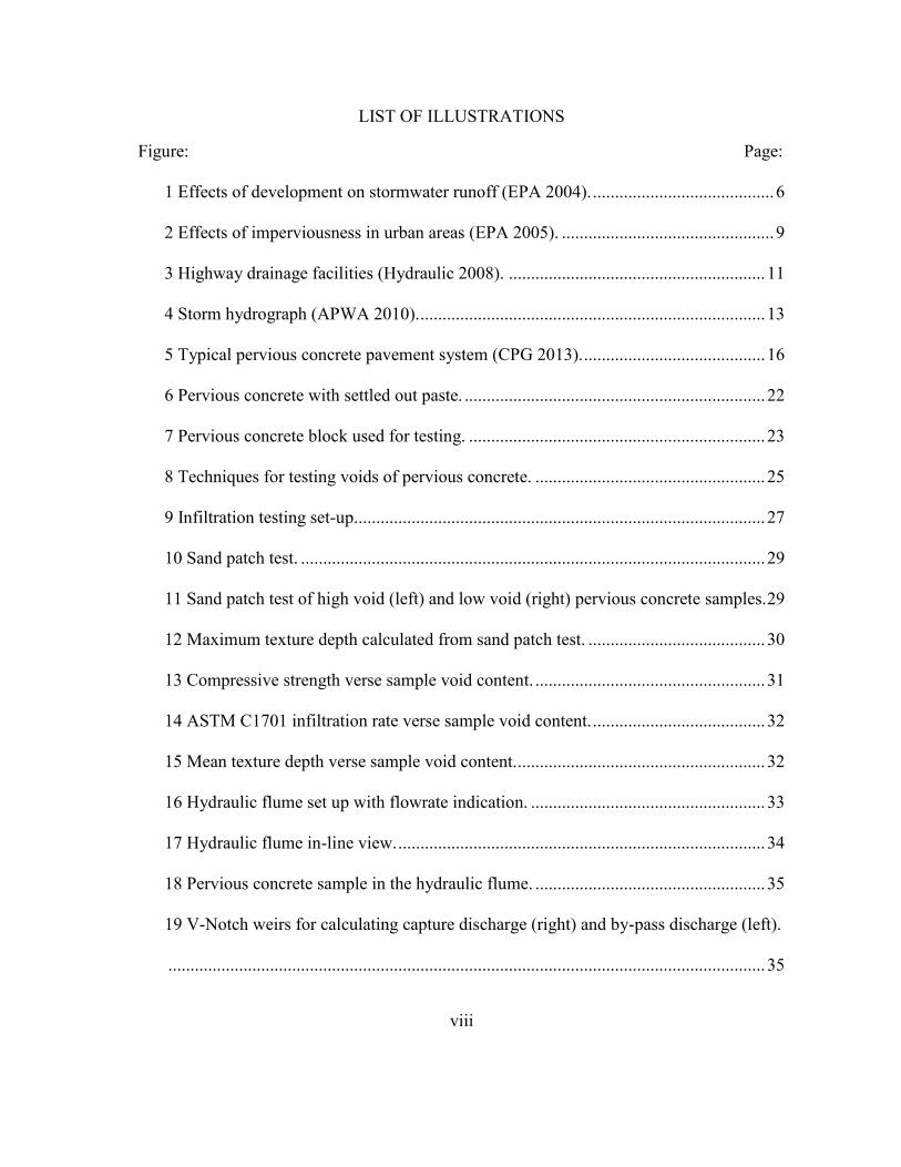
runoff of the site (EPA 1983). In addition to the effects on surface water urbanization has
effects on multiple parts of the water cycle, as shown in Figure 2 (EPA 2005).
9
Figure 2 Effects of imperviousness in urban areas (EPA 2005).
Due to urbanization a significant portion of the water cycle is being transferred into
surface water runoff as seen in Figure 2. This water is transferred into stormwater
conveyance systems before discharge into surface water bodies.
Highway Drainage Design
Stormwater has been an issue ever since roadways have been around. In the early
days when the majority of roads were unpaved, dirt roadways, one substantial storm event
could leave the dirt roads un navigable. These primitive roads made interstate travel a
tedious and time consuming process. Since the 19th
century roadways were recognized as

10
state and local responsibilities, and since privately owned railroads were the primary
source of interstate commerce roadways were the least of state’s concerns (Weingroff
1996).
With the introduction of the Model T, by Henry Ford, in 1908, and the popularity
of bicycles growing the condition of roadways started to become a concern. Farmers
wanted all-weather roads so they could get their products to market, and the automobile
industry wanted hard surfaced interstate roads (Weingroff 1996, 1). With the pressure from
farms, automobile industries, and other activist groups, congress began to investigate
options for federal funding of interstate roadways. After lengthy investigations and
legislative options congress approved the Federal Aid Road Act, and President Wilson
signed the bill in 1916 (Weingroff 1996, 1). Even with the federal funding for roadways
under the Federal Aid Road Act in 1916, dirt and muddy roadways were still common in
the 1930s (Weingroff 1996, 3).
Several legislations were passed and organizations were formed but it wasn’t until
the passing of the Federal-Aid Highway Act of 1956 that uniform interstate design
standards were set in place (Weingroff 1996, 2). The standards set in the 1956 Federal-Aid
Highway Act accommodated for traffic forecasts for 1975 (Weingroff 1996, 2). Ten years
later the Federal Highway Administration (FHWA) was created. The Department of
Transportation Act of 1966 changed the name of the Bureau of Public Roads to the Federal
Highway Administration (FHWA) (Weingroff 1993). The primary goal of the FHWA was
the completion of the interstate system, but there are several other responsibilities of the
FHWA (Weingroff 1993).

11
The FHWA has published numerous documents detailing highway design
guidelines, including hydraulic design of highways. In highway hydraulics there are two
components that must be accounted for which are hydrology and hydraulics (FHWA
2008). The hydrologic aspect accounts for the quantity and frequency of the runoff, surface
water, and ground water (FHWA 2008). The hydraulic aspect accounts for the design of
structures to collect and transport storm water off and away from highway right-of-ways
(FHWA 2008). There are two categories for highway drainage facilities, open channel or
closed conduit facilities (FHWA 2008). Open channel of closed conduit facilities can be
used individually or together, Figure 3 shows an example of the two systems working
together. In figure 3 the roadway channel and median swale represent open channel
drainage facilities, while the median inlet and culvert represent closed conduit facilities.
Figure 3 Highway drainage facilities (Hydraulic 2008).

12
FHWA’s Hydraulic Design Series (HDS) No. 4 states the primary purpose of
highway drainage facilities is to “prevent surface runoff from reaching the roadway and to
remove rainfall or surface water efficiently from the roadway (FHWA 2008).” In order to
fully capture and transport stormwater from roadways, calculation to determine flow rates
into the system must be performed. The first step in calculating stormwater flow rates is to
determine the appropriate flood frequency. After this flood frequency is verified to be
acceptable for design, the flow need to be captured is calculated using the time of
concentration, rainfall intensity, and storm duration (ACI 2010).
The time of concentration is the amount of time that it takes for water from the
storm entering the watershed is equal to the discharge leaving the watershed, entering the
storm sewer system (FHWA 2008).
The calculation of the quantity of water the facility must convey may at first seem
tedious and labor intensive, but there are proven and sound design procedures that are
suitable for more day-to-day design problems (FHWA 2008).
In every storm there is a peak discharge, or a max discharge, this is the discharge
generally used in design calculations. Figure 4 shows a typical hydrograph for a storm
event, indicating the peak flow, and the time to peak flow. The peak rate of runoff can be
calculated using the drainage area and average rainfall intensity, assuming a uniform rate
of intensity (FHWA 2008).

13
Figure 4 Storm hydrograph (APWA 2010).
After calculating the amount of storm runoff needed for capture, the design can be
focused on the hydraulics, or the system used to capture and convey the stormwater.
Although a majority of rural highways use open air drainage channels to convey storm
water away from the site, some highways require close-conduit drainage facilities.
The drainage channels used need to be designed to adequately convey the design
discharge capacity, and are usually lined with vegetation, with rock or paved linings being
utilized where vegetation will not control erosion (AASHTO 2011). Fill slopes are used to
direct storm water from the highway shoulder into drainage channels. When the fill slopes
are subjected to erosion concerns due to the runoff from the roadway, closed conduit
systems are implemented (AASHTO 2011).
Closed conduit systems include the use of dikes, inlets, and chutes of flumes, and
are more suitable for urban highway applications (AASHTO 2011). Typical closed conduit
systems utilize curb and gutter to transport water from the roadway surface to drainage

14
inlets. Drainage inlets on highways should be located appropriately to prevent the spread
of water from entering more than a reasonable distance into the traveled way (AASHTO
2011). Due to the amount of traffic and the speeds of traffic on highways, the allowable
spread width is significantly smaller then on residential roadways (FHWA 2008). Drainage
inlets generally operate under weir flow conditions and are designed based on type,
location (on grade or in a sag), the gutter design, and to operate while partially clogged
(FHWA 2008).
In addition to stormwater conveyance systems, the peak flow can be dramatically
reduced by providing detention basins. Detention basins are especially beneficial when
designing highway drainage where the existing downstream drainage facilities are
inadequate (AASHTO 2011).
Pervious Concrete as a BMP
As discussed earlier there is a strong correlation between landscape perviousness
and surface water runoff. With that theory an ideal option would be to increase surface
perviousness to reduce runoff on highways. The sustainability of pervious concrete has
transformed it into a viable Best Management Practice (BMP). Pervious concrete has been
around for hundreds of years, but was not brought to the United States until after World
War II (CPG 2013).
Pervious concrete is a specialty concrete where the amount of fine aggregate is
either significantly reduced or eliminated, to allow water to intentionally pass through the
surface of the pavement and through the voids (CPG2013). Pervious concrete contains and

15
filters stormwater making it an ideal on site BMP for stormwater management. If this
stormwater can be treated on site through the pervious concrete, the need of conveying
stormwater to water treatment plants is eliminated, and in return eliminates the need to
treat this stormwater. When pervious concrete is used in regions with large amounts of clay
soils, the pervious concrete is placed on a larger rock base to create a stormwater system
(CPG 2013). The use of the rock base and pervious concrete over clay soils allows for a
detention area (in the rock base) for stormwater. These systems have been shown to lose
0.75 inches of water a day to evaporation, this means that a three inch storm event will
evaporate in four days (CPG 2013). Hydrological factors to consider when determining
pervious concrete affects for stormwater are: how much water needs to be mitigated, how
much water will the rock base hold, and how thick of a base should be used (generally 12
inches) (CPG 2013). If the pervious concrete structure can’t mitigate the complete amount
of flow associated with the design flood frequency, overflow pipes can be utilized. These
overflow pipes can connect the concrete to other BMPs such as bioswales or to
conventional stormwater sewer systems (CPG 2013). The use of pervious concrete over
other conventional BMPs’ is optimal due to its help in achieving Low Impact
Developments, where you build up, keeping everything onsite, as opposed to building out
(CPG 2013).
Other benefits in addition to water detention from pervious concrete are: water
filtration, pervious concrete improves the health of trees, recharges ground water aquifers,
reduces pavement effects on urban heat island, and contributes to site LEED accreditation
(Carlson 2007).

16
Like any new hot topic in construction, pervious concrete had to prove itself.
Pervious concrete in the United States began in Florida and other southern coastal states
and slowly migrated to other states with different acceptance and rejection (CPG 2013).
With pervious concrete gaining acceptance in the coastal communities, there was hesitation
for it to migrate to use in the Midwest. This hesitation was largely due to the freeze and
thaw susceptibility of pervious concrete and it’s abilities to withstand the harsher climates
(CPG 2013).The voids in pervious concrete allow water to freely flow through it, therefore
preventing the concrete from breaking apart due to the expansion of water when freezing.
This resistance to breaking up during freeze thaw cycles makes pervious concrete more
desirable than conventional concrete (CPG 2013). This system can be seen in Figure 5,
below.
Figure 5 : Typical pervious concrete pavement system (CPG 2013).

17
There are four main parts to the successful implementation of pervious concrete as
a stormwater BMP, which are: the design of the pavement, the mixture design delivered by
the ready mix producer, the contractor placing the pervious concrete, and the owner with
regards to maintenance of the pavement (CPG 2013). Traditional concrete has been put
through all of the tests and therefore contractors and producers know how to design handle
and construct with traditional concrete. But pervious on the other hand has not been put
through as many tests and contractors and producers are not as familiar with it. This
unfamiliarity leads to numerous problems with the quality of pervious concrete both in the
mixture and in the placement. Special car should be taken when placing pervious concrete.
The low water content and higher void content of pervious concrete make
construction with it more difficult. With pervious concrete there is a correlation between
strength and permeability, as the permeability decreases the strength increases, and vice-
versa. This correlation requires stricter control of the mixture proportioning. The low water
content of pervious concrete also requires transportation and placing times to be lower, to
prevent the concrete from setting before it’s in place. Pervious concrete also requires
special consideration when placing it. Pervious concrete is not pumpable which makes the
logistics of placing it more difficult. Placement of pervious concrete should be continuous
and have rapid spreading, as well as rapid strikeoff (Kevern 2008). Finishing is not
required with pervious concrete; once it is compacted it is finished and can be cured.
If the proper care and attention are put into the design, production, and maintenance
of the pervious concrete pavement are taken, it can be a very successful stormwater BMP.

18
As familiarity and knowledge of pervious concrete continues to grow, so will the use and
implementation of pervious concrete for sustainability.
19
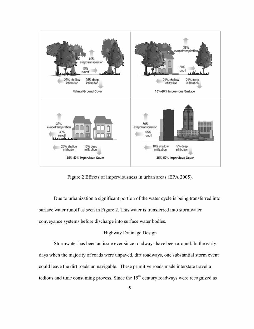
CHAPTER 3
PERVIOUS CONCRETE DESIGN AND TESTING
Materials
The materials used in the pervious concrete mixture were locally available, standard,
materials. The coarse aggregate was an ASTM C33 size #8 crushed limestone with a dry-
rodded void content of 40% (ASTM 2011). A polycarboxylate high-range water reducing
agent was used at 4 oz/cwt (2.5 mL/kg). The unit cwt associated with the high-range water
reducing agent stands for century weight, the 4oz/cwt indicates that there was 4 ounces per
100 pounds of cementitious material in the mixture.
Mixture Design
For testing to fully analyze pervious concrete, a broad range a void contents were
tested. To achieve this goal a broad range of concrete mixtures were designed by void
content. Several mixtures were placed and analyzed, and three of those mixtures were
selected for further testing. The initial mixture utilized different compaction techniques to
achieve various void contents. The void contents achieved from this mixture are: 20%,
35%, and 45%. The mixture proportions for the 20%, 35%, and 45%, samples are shown
in Table 1.

20
Table 1 Pervious Concrete Mixture for the 20%, 35%, and 45% Void Samples.
lb/yd3 kg/m
3
Coarse Aggregate 2620 1555
Portland Cement 550 325
Water 160 95
To fill out the range of void contents mixture designs utilizing higher paste contents
were investigated. The additional amount of paste created lower voids. Several mixtures
were placed utilizing different amounts of paste, with varying results. Two of these
mixtures were produce void contents of 15% and 25% and were chosen for further
investigation. The mixture designs for sample void contents 15% and 25% are shown in
Tables 2 and 3, respectively.
Table 2 Pervious Concrete Mixture for the 15% Void Sample.
lb/yd3 kg/m
3
Coarse Aggregate 2450 1110
Portland Cement 650 295
Water 195 90

21
Table 3 Pervious Concrete Mixture for the 25% Void Sample.
lb/yd3 kg/m
3
Coarse Aggregate 2530 1150
Portland Cement 600 270
Water 180 80
Several of the mixture designs utilizing additional amounts of paste were too fluid
and not pervious enough for testing. With higher paste pervious concrete designs there is a
chance that the paste will separatefrom the mixture. This occurred with several mixtures
tested and an example is shown in Figure 6. In Figure 6 it is apparent that a majority of the
paste settled to the bottom of the sample.

22
Figure 6 Pervious concrete with settled out paste.
Samples
Nine cylinders and three test blocks were placed of each sample type, for testing of
the concrete properties in triplicate. Mixing and curing of the concrete samples was
performed in accordance with ASTM C192 (ASTM 2007). The blocks were 14 in. by 14
in. by 3 in. (355.6 mm x 355.6 mm x 76.2 mm) to allow infiltration testing per ASTM
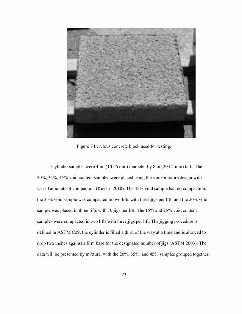
C1701 (ASTM 2009). An example of these blocks is shown in Figure 7. As shown in
Figure 7, the sides are the samples were sealed with duct tape to ensure the water
infiltrated through the sample.
23
Figure 7 Pervious concrete block used for testing.
Cylinder samples were 4 in. (101.6 mm) diameter by 8 in (203.2 mm) tall. The
20%, 35%, 45% void content samples were placed using the same mixture design with
varied amounts of compaction (Kevern 2010). The 45% void sample had no compaction,
the 35% void sample was compacted in two lifts with three jigs per lift, and the 20% void
sample was placed in three lifts with 10 jigs per lift. The 15% and 25% void content
samples were compacted in two lifts with three jigs per lift. The jigging procedure is
defined in ASTM C29, the cylinder is filled a third of the way at a time and is allowed to
drop two inches against a firm base for the designated number of jigs (ASTM 2003). The
data will be presented by mixture, with the 20%, 35%, and 45% samples grouped together,

24
and then the 25% and 15% samples. Fresh unit weight was measured on the cylinders and
the appropriate amount massed for the slab samples to ensure equal voids.
Void Content
Hardened void content and unit weight was determined according to ASTM C1754
(ASTM C1754 2012). The basic principles and calculations in ASTM C1754 were
modified to allow for the testing of void content on the pervious concrete blocks. Hardened
void content is determined by weighing the samples submerged in water and then dried.
The modifications to ASTM C1754 included modified techniques to obtain the submerged
weight of the concrete blocks. These modifications are shown in Figure 8. The percentages
used for sample identification are the hardened void content of the blocks. The hardened
void content of the cylinders is shown in Table 4.

25
Figure 8 Techniques for testing voids of pervious concrete.
Table 4 Cylinder Void Testing Results
Sample
Cylinder
Voids
Std.
Deviation
45% 47% 0.226%
35% 38% 0.657%
25% 31% 0.670%
20% 25% 0.404%
15% 23% 0.285%
Compressive Strength
Compressive strength was determined at 7 days on sulfur-capped specimens according to
ASTM C39 (ASTM C39 2012). The results of the compressive strength testing are shown
in Table 5.

26
Table 5 Compressive Strength Testing Results
Sample
7 Day Compressive
Strength (psi)
Std.
Deviation
45% 511 41
35% 1070 44
20% 1255 29
25% 2920 47
15% 3160 36
Infiltration
Infiltration of the samples was tested on the blocks in accordance with ASTM C1701
(ASTM 2009). ASTM C1701 is performed by determining the time a specified amount of
water takes to infiltrate the sample. The water is poured onto the sample in a ring with a
predetermined area, from the area of the ring and the time the water takes to infiltrate the
sample, the infiltration rate can be calculated. The procedure for infiltration testing is
considered a constant head test, were a predetermined weight of water is introduced into
the samples at a constant rate. This procedure is shown in Figure 9, and the results are
shown in Table 6.

27
Figure 9 Infiltration testing set-up.
In Figure 9 water is poured into the ring of PVC, and is kept at a determined height to
sustain the constant head, and the time the water takes to penetrate the sample is used to
determine the infiltration in inches per hour.
Table 6 Infiltration Testing Results
Sample Infiltration (in/hr) Std. Deviation
45% 3944 244
35% 1784 65
20% 461 35
25% 781 177
15% 304 98

28
Mean Texture Depth
A sand patch test is used to determine the surface texture of concrete pavements, and was
performed in accordance with ASTM E965 (ASTM E965 2006). The procedure to
determine surface texture of concrete pavements includes spreading, in a circular pattern, a
pre-determined volume of standard sand. From the diameter of the circle the surface
texture can be calculated using the equation below.
;
Where,
MTD = Mean Texture Depth, in (mm),
V = Sample volume of sand, in3 (mm
3),
And,
D = Average diameter of the area covered by standard sand.
Figure 10 shows the sand before spreading and after spreading. And Figure 11 shows the
difference, in spread, between a high void sample (on the left) and a low void sample (on
the right). Figure 11 depicts that the higher void sample has a smaller spread, due to the
sand penetrating through the increased amount of voids, while, the lower void sample
indicates a larger spread, due to lack of voids.

29
Figure 10 Sand patch test.
Figure 11 Sand patch test of high void (left) and low void (right) pervious concrete
samples.
BEFORE
HIGH LOW
AFTER

30
The calculated MTDs of the sand patch test are shown in Figure 12.
Figure 12 Maximum texture depth calculated from sand patch test.
Summarized Testing Results
Table 7 shows a summary of all the determined concrete properties.
Table 7 Summarized Concrete Properties
Sample
Cylinder
Void, %
7 Day
Compressive
Strength, psi
ASTM
C1701
Infiltration
(in/hr)
Mean
Texture
Depth, in
45% 0.47 511 3950 0.30
35% 0.38 1070 1790 0.11
20% 0.31 1255 460 0.06
25% 0.25 2920 780 0.10
15% 0.23 3160 300 0.06
0.30
0.11
0.06
0.099
0.06
0.00
0.05
0.10
0.15
0.20
0.25
0.30
0.35
MTD
, in
45% 35% 20% 25% 15%

31
Figures 13, 14, and 15 show the compressive strength, infiltration rate, and mean
texture depth verse the sample void content, respectively. The figures showing the
infiltration rate and the mean texture depth show the results as expected. The spike in data
shown in Figure 13 is due to the different mixture design used to obtain the range of voids.
Figure 13 Compressive strength verse sample void content.
0
500
1000
1500
2000
2500
3000
3500
10% 15% 20% 25% 30% 35% 40% 45% 50%
7 D
ay C
om
pre
ssiv
e S
tre
ngt
h, p
si
Sample Voids Content, %

32
Figure 14 ASTM C1701 infiltration rate verse sample void content.
Figure 15 Mean texture depth verse sample void content.
0
500
1000
1500
2000
2500
3000
3500
4000
4500
10% 15% 20% 25% 30% 35% 40% 45% 50%
AST
M C
17
01
In
filt
rati
on
, in
/hr
Sample Voids Content, %
0
0.05
0.1
0.15
0.2
0.25
0.3
0.35
10% 15% 20% 25% 30% 35% 40% 45% 50%
Me
an T
ext
ure
De
pth
, in
Sample Voids Content, %

33
CHAPTER 4
HYDRAULIC TESTING
A hydraulic flume was designed and constructed to analyze hydraulic flow across
the samples at different slopes and flow rates. The flume used for testing is shown in
Figure 16. The flow rate was verified in triplicate. An in-line Venturi meter to measure the
total flow rate (QTOTAL) into the system and two V-notch Weirs were used to measure the
captured discharge (water flowing through the sample, QINFILTRATION), and the by-pass
discharge (water flowing over the sample, QBY-PASS). Figure 17 shows an in-line view of
the flume.
Figure 16 Hydraulic flume set up with flowrate indication.

34
Figure 17 Hydraulic flume in-line view.
The pervious concrete samples were placed in the hydraulic flume and sealed
around the edges to prevent water from infiltrating through the edges between the concrete
and the model. Standard plumbers putty was used to seal the edges. Figure 18 shows the
pervious concrete block in the flume. Also in Figure 18 are four screws located in the
corners of the sample. These screws were used for installation and removal of the sample.
The V-notch weirs were constructed from a piece of an eighth inch (3.175 mm)
aluminum, and the notches were cut at a 22.5 degree angle, shown in Figure 19.
QTOTAL

35
Figure 18 Pervious concrete sample in the hydraulic flume.
Figure 19 V-Notch weirs for calculating capture discharge (right) and by-pass discharge
(left).

36
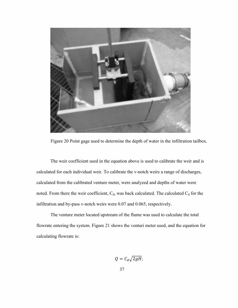
The use of v-notch weirs to determine flowrate requires the depth of water
upstream of the weir. The depth of water upstream of the weir was measured in dead zones
of the tailboxes to minimize the inconstancies associated with turbulent flow. This is
shown in Figure 20, where a point gage was used in the infiltration tailbox to determine
depth of water. The infiltration and by-pass flowrate are calculated using the following
equation:
√ ⁄ ; (eq. 1)
Where,
Q = Flowrate, cfs,
Cd = Weir Coefficient,
g = gravity, 32.2 ft/s2
and
H = Height of water upstream of the weir, in.
37
Figure 20 Point gage used to determine the depth of water in the infiltration tailbox.
The weir coefficient used in the equation above is used to calibrate the weir and is
calculated for each individual weir. To calibrate the v-notch weirs a range of discharges,
calculated from the calibrated venture meter, were analyzed and depths of water were
noted. From there the weir coefficient, Cd, was back calculated. The calculated Cd for the
infiltration and by-pass v-notch weirs were 0.07 and 0.065, respectively.
The venture meter located upstream of the flume was used to calculate the total
flowrate entering the system. Figure 21 shows the venturi meter used, and the equation for
calculating flowrate is:
√ ;

38
Where,
Q = flowrate, cfs,
Cd = Weir coefficient,
g = Gravity, 32.2 ft/s2,
and,
H = Height Difference, ft of water.
Where,
H = HIF(SGMerrium – 1)
HIF = Height difference of dye in the venture, ft,
SGMerrium = Specific gravity of merrium dye, 2.95
Figure 21 Venturi meter used for calculating flowrate into the system.
.

39
Highways and roadways have various slopes, to analyze field applications of the
pervious concrete the slopes of different roadways needed to be mimicked. A hydraulic
jack was used to vary the slope of the flume, and is shown in Figure 22. A full range of
slopes were chosen for testing and they were: 0%, 0.5%, 1.0%, 2.0%, 5.0%, and 10.0%.
Figure 22 Hydraulic jack used to alter the slope of the flume.
The flume was designed to maintain a constant sheet flow of water through the
flume. This water was flowing at subcritical velocities and is shown in Figure 23.

40
Figure 23 Steady flow of Water at Subcritical Velocities.

41
CHAPTER 5
RESULTS AND DISCUSSION (UNCLOGGED)
Maximum Capture Flowrate
The results presented in this chapter are for the hydraulic response of unclogged permeable
pavements. Each sample was tested at six different slopes, across a range of flow rates.
Figure 24 shows a performance curve for the high void samples at a 0% cross slope. The
performance curve shown in Figure 24 is typical for all the samples. As the flow rate
increases so does infiltration until by-pass occurs. A small increase in observed infiltration
occurs as the flow depth increases until the pavement reaches a point of maximum
consistent infiltration. After the point of consistency is reached the infiltration rate
becomes independent flow rate.

42
Figure 24 Explanation of a typical performance curve
A performance curve was plotted for each block, void content, and slope, for a total
of ninety performance curves. All plots were similar in nature and the plot shown at each
void content for a 0% cross slope in Figures 25 through 29. The point of by-pass shown on
Figure 24, was selected as the maximum capture flowrate for design calculations. That is
the maximum amount of flow that will infiltrate the sample before overflow occurs.
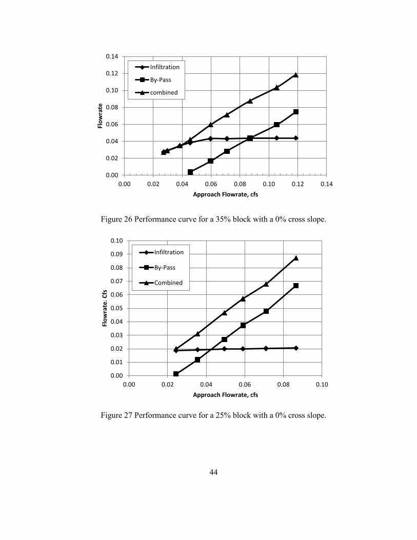
The performance curves shown in Figures 25 through 29 indicate that as the void
content is reduced, the amount of infiltration is also reduced, as expected. The performance
curves also show the tendency of the amount of infiltration levels off, and reach a
maximum infiltration flowrate, or Maximum Capture Flowrate. It is important to note that
0.00
0.02
0.04
0.06
0.08
0.10
0.12
0.14
0.16
0.18
0.20
0.00 0.05 0.10 0.15 0.20
V-n
otc
h F
low
Rat
e, c
fs
Venturi Flow rate, cfs
Infiltration
By-pass Discharge
Combined Discharge
Point of by-pass
Hydraulic Head = 0.47 in. (11.9mm)

43
at higher void contents the infiltration gradually increases before reaching MCF, while at
the lower void contents the infiltration reaches MCF immediately, as seen in Figures 27,
28, and 29. While the main focus of this thesis is the flowrate at which the by-pass begins,
the MCF’s of the specimens are important and Table 8 shows the MCF for the samples.
The information in Table 8 is an average of the three blocks for each slope and void
content. Figure 30 is a plot of the data represented in Table 8.
Figure 25 Performance curve for a 45% block with a 0% cross slope.
0.00
0.02
0.04
0.06
0.08
0.10
0.12
0.14
0.16
0.18
0.20
0.00 0.05 0.10 0.15 0.20
Flo
w R
ate
, cfs
Approach Flow rate, cfs
Infiltration
By-passDischarge
CombinedDischarge
44
Figure 26 Performance curve for a 35% block with a 0% cross slope.
Figure 27 Performance curve for a 25% block with a 0% cross slope.
0.00
0.02
0.04
0.06
0.08
0.10
0.12
0.14
0.00 0.02 0.04 0.06 0.08 0.10 0.12 0.14
Flo
wra
te
Approach Flowrate, cfs
Infiltration
By-Pass
combined
0.00
0.01
0.02
0.03
0.04
0.05
0.06
0.07
0.08
0.09
0.10
0.00 0.02 0.04 0.06 0.08 0.10
Flo
wra
te. C
fs
Approach Flowrate, cfs
Infiltration
By-Pass
Combined

45
Figure 28 Performance curve for a 20% block with a 0% cross slope.
Figure 29 Performance curve for a 15% block with a 0% cross slope.
0.00
0.02
0.04
0.06
0.08
0.10
0.12
0.00 0.02 0.04 0.06 0.08 0.10 0.12
Flo
wra
te, c
fs
Approach Flowrate, cfs
Infiltration
By-Pass
combined
0.00
0.01
0.02
0.03
0.04
0.05
0.06
0.07
0.08
0.09
0.10
0.00 0.02 0.04 0.06 0.08 0.10
Flo
wra
te, c
fs
Approach Flowrate, cfs
Infiltration
By-Pass
Combined

46
Table 8 Maximum Capture Flowrates
Void
Content
Pavement Cross Slope
0% 0.5% 1% 2% 5% 10%
45% 0.108 0.109 0.110 0.109 0.107 0.104
35% 0.053 0.052 0.052 0.051 0.049 0.048
25% 0.022 0.021 0.021 0.020 0.020 0.020
20% 0.013 0.012 0.011 0.011 0.011 0.010
15% 0.007 0.007 0.006 0.006 0.005 0.005
*Values are in cfs
Figure 30 Plot of pavement cross slope verse flowrate for the range of voids.
The data represented in Table 8 verifies that for any slope the MCF will
significantly reduce as the void content is reduced. The data in Table 8 also shows that as
the pavement cross slope is increased for any of the void contents the MCF does not have a
significant change.
Maximum Capture Flowrate before By-Pass
0.00
0.02
0.04
0.06
0.08
0.10
0.12
0% 2% 4% 6% 8% 10% 12%
Flo
wra
te, c
fs
Pavement Cross Slope, %
45% Voids
35% Voids
25% Voids
20% Voids
15% Voids

47
The performance curves were used to calculate a Maximum Capture Flowrate
before ByPass (MCFPB) for each concrete block at each cross slope. To determine the
MCFBP a linear trendline of the by-pass discharge line, seen in Figure 24, was used. The
equation of the trendline of the by-pass discharge line was used to back calculate the point
where by-pass began (where the trendline intercepts the x-axis), and this point is the
MCFBP. The MCFBP’s calculated for each respective void content are shown in Tables 9
through 13.
Table 9 MCFBP for 45% Void
Slope
Block (cfs)
1 2 3
0% 0.089 0.120 0.107
0.5% 0.092 0.111 0.095
1% 0.089 0.104 0.090
2% 0.083 0.104 0.093
5% 0.073 0.095 0.092
10% 0.072 0.086 0.084
*Values are in cfs
Table 10 MCFBP for 35% Void Content
Slope
Block (cfs)
1 2 3
0% 0.042 0.059 0.051
0.5% 0.037 0.056 0.048
1% 0.043 0.050 0.052
2% 0.034 0.049 0.045
5% 0.026 0.045 0.046
10% 0.022 0.038 0.040
*Values are in cfs

48
Table 11 MCFBP for 25% Void Content
Slope
Block (cfs)
1 2 3
0% 0.024 0.026 0.024
0.5% 0.019 0.022 0.020
1% 0.018 0.021 0.016
2% 0.018 0.023 0.016
5% 0.018 0.022 0.016
10% 0.016 0.023 0.012
*Values are in cfs
Table 12 MCFBP for 20% Void Content
Slope
Block (cfs)
1 2 3
0% 0.016 0.016 0.018
0.5% 0.014 0.011 0.013
1% 0.011 0.013 0.012
2% 0.012 0.010 0.014
5% 0.011 0.011 0.010
10% 0.005 0.009 0.008
*Values are in cfs
49
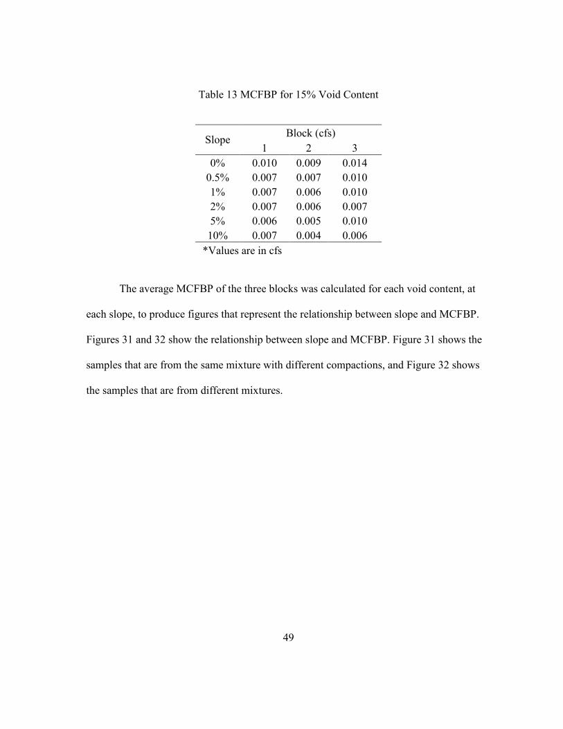
Table 13 MCFBP for 15% Void Content
Slope
Block (cfs)
1 2 3
0% 0.010 0.009 0.014
0.5% 0.007 0.007 0.010
1% 0.007 0.006 0.010
2% 0.007 0.006 0.007
5% 0.006 0.005 0.010
10% 0.007 0.004 0.006
*Values are in cfs
The average MCFBP of the three blocks was calculated for each void content, at
each slope, to produce figures that represent the relationship between slope and MCFBP.
Figures 31 and 32 show the relationship between slope and MCFBP. Figure 31 shows the
samples that are from the same mixture with different compactions, and Figure 32 shows
the samples that are from different mixtures.

50
Figure 31 MCFBP for the 45%, 35%, and 20% voids samples
Figure 32 MCFBP for the 25% and 15% voids samples.
0.00
0.02
0.04
0.06
0.08
0.10
0.12
0% 2% 4% 6% 8% 10% 12%
Max
imu
m C
aptu
re F
low
rate
, cfs
Slope, %
45% Voids
35% Voids
20% Voids
0.00
0.01
0.01
0.02
0.02
0.03
0.03
0% 2% 4% 6% 8% 10% 12%
Max
imu
m C
aptu
re F
low
rate
, cfs
Slope, %
25% Voids
15% Voids

51
The data displayed in Figures 31 and 32 show trends that indicate as the cross slope
of the pervious concrete blocks increases the MCF decreases.
Effective Intensity
To provide a standard that could be used for design of pervious concrete highway
shoulders the MCFBP from the model was converted to an effective intensity. The
effective intensity is the maximum flowrate the pervious concrete can handle per unit
length per unit width. To convert the model MCFBP into an effective intensity the
equation below was used.
(
);
Where,
IE = Effective Intensity, cfs,
MCFBP = Mean Capture Flowrate before By-Pass, cfs,
LM = Length of the section used in the model, ft,
AndWM = Width of the Concrete block used in the model, ft.
The calculated effective intensities are shown in Tables 14. The behavior of the
effective intensities mirrors the behavior of the MCFBP, due to the direct relationship.

52
Table 14 Effective Intensities for Varied Slopes
Slope
Effective Intensity, cfs
45%
Voids
35%
Voids
25%
Voids
20%
Voids
15%
Voids
0.0% 0.0762 0.037 0.014 0.012 0.008
0.5% 0.0718 0.034 0.013 0.009 0.006
1.0% 0.0684 0.035 0.012 0.009 0.006
2.0% 0.0678 0.031 0.012 0.009 0.005
5.0% 0.0627 0.028 0.009 0.008 0.005
10.0% 0.0584 0.024 0.009 0.005 0.004
Infiltration
Water flows across pavements in sheet flow, which is supercritical flow. Super
critical flow has a higher velocity than normal flow (Bedient 2008). Data collected from
this research has shown that infiltration observed during sheet flow across a pavement is
lower than infiltration rates measured by ASTM C1701, on the same pavement (ASTM
C1701 2009). ASTM 1701 uses a constant head test to determine pervious concrete’s
infiltration rate. The infiltration rates calculated by ASTM 1701 are shown in Chapter 3.
ASTM C1701 calculates infiltration based on standing water on the pavement, while the
model calculates infiltration based on sheet flowing water across the pavement. The
majority of pervious concrete pavements are specified based on its infiltration rate, and is
expected to meet that rate when it’s installed.
The relationship between the ASTM 1701 infiltration rate and the MCFBP
(Capture Discharge) is shown in Figure 33. Figure 33 provides a visual on the relationship
between the ASTM 1701 infiltration rate and the MCBP, the capture discharge. Figure 33
shows two trends, first that as the slope increases the MCFBP decreases, and this is as
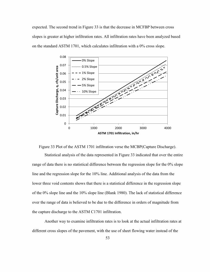
53
expected. The second trend in Figure 33 is that the decrease in MCFBP between cross
slopes is greater at higher infiltration rates. All infiltration rates have been analyzed based
on the standard ASTM 1701, which calculates infiltration with a 0% cross slope.
Figure 33 Plot of the ASTM 1701 infiltration verse the MCBP(Capture Discharge).
Statistical analysis of the data represented in Figure 33 indicated that over the entire
range of data there is no statistical difference between the regression slope for the 0% slope
line and the regression slope for the 10% line. Additional analysis of the data from the
lower three void contents shows that there is a statistical difference in the regression slope
of the 0% slope line and the 10% slope line (Blank 1980). The lack of statistical difference
over the range of data is believed to be due to the difference in orders of magnitude from
the capture discharge to the ASTM C1701 infiltration.
Another way to examine infiltration rates is to look at the actual infiltration rates at
different cross slopes of the pavement, with the use of sheet flowing water instead of the
0
0.01
0.02
0.03
0.04
0.05
0.06
0.07
0.08
0 1000 2000 3000 4000
Cap
ture
Dis
char
ge, q
, cfs
/un
it a
rea
ASTM 1701 Infiltration, in/hr
0% Slope
0.5% Slope
1% Slope
2% Slope
5% Slope
10% Slope

54
constant head method utilized by ASTM 1701. The infiltration rate observed by the model
was calculated from the effective intensities. To convert effective intensities into
infiltration rate, a simple unit transformation was performed. Effective intensities are in cfs
and infiltration rates need to be in inches per hour, thus, multiplying the effective
intensities by 43,200 (3600 seconds/hour times 12inches/foot) will produce infiltration
rates. The calculated infiltration rates at by-pass are shown in Table 15. The infiltration
rates shown in Table 15 are average values of three blocks, and are based off the MCFBP.
Table 15 Infiltration Rates at the By-Pass Flow
Slope
Infiltration Rate, in/hr
45%
Voids 35% Voids
25%
Voids
20%
Voids
15%
Voids
0.0% 3300 1590 770 520 330
0.5% 3100 1470 630 400 250
1.0% 3000 1510 580 390 240
2.0% 2900 1340 600 390 210
5.0% 2700 1220 580 330 220
10.0% 2500 1040 530 220 170
Tables 15 shows a relationship between slope and infiltration. As the slope is
increased the infiltration rate decreases. The infiltration rates of the different void contents
will decrease similarly to the MCF’s shown in Figure 33, due to the direct relationship of
the infiltration and the MCF.
Figure 34 shows the actual infiltration verse infiltration determined by ASTM
C1701, for the same high void sample at a horizontal slope (ASTM 2009). For very low

55
infiltration values the difference is small, but as the run-on velocity increases there is a
substantial reduction in the infiltration capacity.
Figure 34 Actual infiltration verse ASTM C1701 infiltration.
0
500
1000
1500
2000
2500
3000
3500
4000
0 500 1000 1500 2000 2500 3000 3500 4000
Act
ual
Infi
ltra
tio
n, i
n/h
r
ASTM 1701 Infiltration, in/hr
0% Cross Slope
0.5% Cross Slope
1.0% Cross Slope
2.0% Cross Slope
5.0% Cross Slope
10.0% Cross Slope

56
CHAPTER 6
RESULTS AND DISCUSION (CLOGGED)
In regions that have cold climates , it is crucial for roadways to be treated for icy
and slick conditions during inclement weather. To reduce the buildup off ice on roadways
and provide traction for motorists a combination of deicers and sand is generally used.
While the deicers themselves are generally not a problem with regards to clogging of
pervious concrete, the deicers is either liquid or a substance able to dissolve. The sand
used in deicing could infiltrate and clog the pervious concrete used in highway shoulders.
This chapter will discuss how the model was used to mimic de-icing treatments and the
results generated.
The amount of sand used in the model was calculated based off a few general
assumptions. The first assumption made was that the design would be for a two lane, 12
feet per lane, highway. The second assumption was a spread rate of 600 pounds per lane
per mile of de-icing mixture. And the third assumption was a deicing mixture ratio of 1:1
salt to sand. These assumptions were based off of amounts used in Massachusetts and
Wisconsin (Massachusetts 2006, Walker 2005).
In the model sand was initially spread upstream of the pervious concrete blocks and
allowed to be suspended in the water and carried into the sample. This method is shown in
Figure 35. Due to the techniques used to secure the pervious concrete blocks in the model

57
the sand would become trapped before entering the concrete. The entrapped sand can be
seen in Figure 36. To mitigate this problem the sand was windrowed on the upstream most
part of the pervious concrete blocks, this is shown in Figure 37. Figure 38 shows how the
sand clogged the pervious concrete blocks. The larger pieces of sand are more visible on
the top layer while the smaller pieces of sand infiltrated deeper into the block.
Figure 35 Sand spread upstream of pervious concrete block.
QTOTAL

58
Figure 36 Entrapped sand upstream of pervious concrete block
Figure 37 Sand windrowed at upstream-most part of pervious concrete block

59
Figure 38 Sand clogging the pervious concrete block.
The hydraulic flume was modified for the clogging tests and was fixed at a 2%
cross slope to simulate a roadway. Initial clogging testing involved recording data after
each dosage rate to identify if there is a trend. The MCF was calculated the same way as
described in Chapter 5. Figures 39 and 40 show the effects of deicers, per application, have
on the MCF. Figure 39 is data for one of the 25% void content blocks. Figure 40 is data for
one of the 20% void content blocks.

60
Figure 39 Plot of applications of sand verse MCF for 25% void content block.
Figure 40 Plot of applications of sand verse MCF for the 20% void content block.
0
0.002
0.004
0.006
0.008
0.01
0.012
0.014
0.016
1 2 3 4 5 6 7 8 9 10 11 12 13 14 15 16 17
Max
imu
m C
aptu
re F
low
rate
, cfs
Applications of Sand
0
0.002
0.004
0.006
0.008
0.01
0.012
0.014
1 2 3 4 5 6 7 8 9 10 11 12 13 14
Max
imu
m C
aptu
re F
low
rate
, cfs
Applications of Sand
61
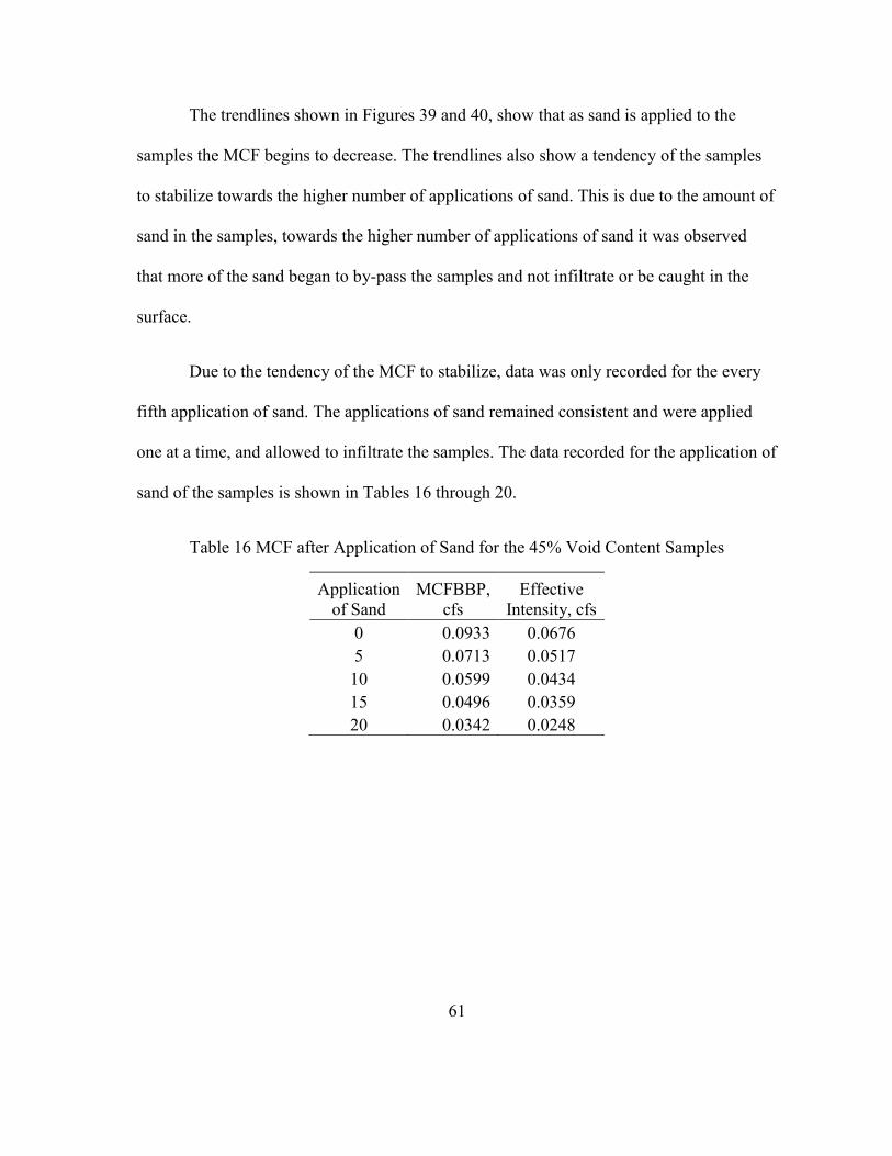
The trendlines shown in Figures 39 and 40, show that as sand is applied to the
samples the MCF begins to decrease. The trendlines also show a tendency of the samples
to stabilize towards the higher number of applications of sand. This is due to the amount of
sand in the samples, towards the higher number of applications of sand it was observed
that more of the sand began to by-pass the samples and not infiltrate or be caught in the
surface.
Due to the tendency of the MCF to stabilize, data was only recorded for the every
fifth application of sand. The applications of sand remained consistent and were applied
one at a time, and allowed to infiltrate the samples. The data recorded for the application of
sand of the samples is shown in Tables 16 through 20.
Table 16 MCF after Application of Sand for the 45% Void Content Samples
Application
of Sand
MCFBBP,
cfs
Effective
Intensity, cfs
0 0.0933 0.0676
5 0.0713 0.0517
10 0.0599 0.0434
15 0.0496 0.0359
20 0.0342 0.0248

62
Table 17 MCF after Application of Sand for the 35% Void Content Samples
Application
of Sand
MCFBP,
cfs
Effective
Intensity, cfs
0 0.0427 0.0309
5 0.0288 0.0209
10 0.0193 0.0140
15 0.0119 0.0086
20 0.0075 0.0054
Table 18 MCF after Application of Sand for the 25% Void Content Samples
Application
of Sand
MCFBP,
cfs
Effective
Intensity, cfs
0 0.0190 0.0138
5 0.0099 0.0071
10 0.0056 0.0041
15 0.0035 0.0025
20 0.0028 0.0020
Table 19 MCF after Application of Sand for the 20% Void Content Samples
Application
of Sand
MCFBP,
cfs
Effective
Intensity, cfs
0 0.012 0.0087
5 0.00463 0.0034
10 0.00283 0.0021
15 0.00175 0.0013
20 0.0012 0.0009

63
Table 20 MCF after Application of Sand for the 15% Void Content Samples
Application
of Sand
MCFBP,
cfs
Effective
Intensity,
cfs
0 0.0067 0.0048
5 0.0027 0.0020
10 0.0015 0.0011
15 0.0008 0.0006
20 0.0006 0.0004
The data shown in Tables 16 through 20 indicate that as the more sand is applied to
the sample the lower the MCF, as expected. The results indicates that as the void content
of the samples decreases so does the final MCFBP. The results also indicate that there is a
greater difference in the initial applications of sand than in the later applications. The
decrease in change between the later applications of sand is due to the void content being
reduced as the sand infiltrates and clogs the sample, forcing more of the sand to by-pass,
and creating a smaller change in the amount of clogged space in the sample. Figure 41
shows the effects of applications of sand on the ASTM C1701 infiltration rate.

64
Figure 41 Infiltration rate verse capture discharge for various applications of sand.
The relationship between infiltration rate and capture discharge shown in Figure 41
behaves as expected from the previous data presented. The capture discharge is shown to
decrease with the additional applications of sand. This decrease in capture discharge is
more substantial as the infiltration rate increases.
Additional Testing
After the final application of sand to the pervious concrete blocks three additional
tests were performed. The tests were performed on one block each, therefore the data
presented in this section is only representative of one block.
The first additional test was to determine if any of the sand that infiltrated the block
would become mobile once the block was dried. To analyze this, the samples were allowed
0.0
0.5
1.0
1.5
2.0
2.5
3.0
3.5
0 500 1000 1500 2000
Cap
ture
Dis
char
ge, q
, cfs
/un
it w
idth
/ u
nit
len
gth
, (x
10
-2)
ASTM C1701 Infiltration Rate, in/hr
Before Sand
5 Applications
10 Applications
15 Applications
20 Applications

65
to completely dry after the final application of sand was added. Once the blocks were
completely dry they were tested again to determine MCFBP. The effects on drying of the
sample on the MCF are shown in Table 21.
Table 21 Effect of Drying on MCF
*MCF Values are in cfs
While the MCF did not return to the original MCF before application of sand, the
data suggests that is allowed to dry the MCF will increase slightly. Further investigation
would be needed to determine the effects of the sample drying in between each application
of sand.
The second additional test performed was to determine the effects of vacuuming the
pervious concrete blocks on the MCF. Typical maintenance of pervious concrete
pavements includes vacuuming to remove debris clogging the pavement. To analyze the
effects of vacuuming the pervious concrete blocks were allowed to completely dry. Once
dry the blocks were vacuumed using a standard shop vacuum with 6.5 peak horsepower.
The effects of vacuuming are shown in Table 22.
After Sand Application After Drying
Void Content Original Clogged
% From Original After Drying
% From Original
45% 0.083 0.0218 -74% 0.0222 -73%
35% 0.034 0.0084 -75% 0.011 -68%
15% 0.007 0.0007 -90% 0.0025 -64%

66
Table 22 Effect of Vacuuming on MCF
After Sand Application After Vacuuming
Void Conctent Original Clogged
% From Original
After Vacuuming
% From Original
45% 0.104 0.0466 -55% 0.0468 -55%
35% 0.049 0.0075 -85% 0.0269 -45%
25% 0.016 0.0025 -84% 0.0112 -30%
20% 0.014 0.0011 -92% 0.0068 -51%
15% 0.007 0.0007 -90% 0.0043 -39%
*MCF Values are in cfs
The effects of vacuuming on the pervious concrete blocks shown in Table 22
indicate similar results to the effects of drying. The results indicate that vacuuming will
increase the MCF. The vacuuming results are also similar to the drying results in that
neither resulted in complete mitigation of the loss of MCF due to clogging. To analyze
which remediation process is more effect the percent loss from before clogging to after
remediation is shown in Table 23. The values shown are the percentage increase of the
MCF due to remediation from the clogged MCF.
Table 23 Comparison of Drying and Vacuuming for Remediating Clogging
Void
Content
% Increase in
MCF from
Vacuuming
% Increase in
MCF from
Drying
45% 0% 2%
35% 260% 30%
25% 350% -
20% 520% -
15% 510% 260%

67
The results shown in Table 23 show a significant increase in MCF due to
remediation for all void contents except the 45%. The effects on the 45% void content
sample are minimal due to the amount of voids. The more voids associated with the 45%
void content sample enabled the sand to infiltrate deeper into the block which made
remediation more difficult.
Table 23 also indicates that as the void content decreases the effects remediation
increase. The increase in effectiveness of remediation is due to the diminishing of voids.
With lower void amounts the sand was not able to infiltrate as deep, leaving a majority of
the sand near the top, making remediation more efficient.
All remediation techniques discussed in this section were implemented after the
completion of the 20th
application of sand. Further investigation of remediation earlier in
the stages of clogging is still needed. But, it is believed that these results will be more
substantial if performed prior to complete clogging of the pervious concrete.

68
CHAPTER 7
HYDRAULIC DESIGN OF PERVIOUS CONCRETE
The laboratory flow rates and discharges were converted into effective rainfall
intensity to correlate the data with design storm frequencies. Rainfall intensity is based on
the duration of rainfall, and the area affected by rainfall (Bedient 2008). The effective
intensities shown in Figure 42 are based on the area of the concrete sample and are shown
as capture discharge (amount of flow that will infiltrate the pavement in cubic feet per
second, per unit width, per unit length). The capture discharge is plotted against the
infiltration rate in Figure 42. Figure 42 shows the linear relationship between the
infiltration rate and the capture discharge. Figure 42 also shows that at increased cross
slopes the relationship between capture discharge and design infiltration remains linear, but
the amount of capture discharge is lower. This is an important relationship because it
verifies the assumption that as slope increases the amount of infiltration decreases.
For ease of design Figure 43 was generated from Figure 42 to show the capture
discharges for varying slopes at lower infiltration rates.

69
Figure 42 Capture discharge verse pavement infiltration rate.
Figure 43 Capture discharge verse pavement infiltration rate, at lower infiltration rates.
0
0.01
0.02
0.03
0.04
0.05
0.06
0.07
0.08
0 1000 2000 3000 4000
Cap
ture
Dis
char
ge, q
, cfs
/un
it a
rea
ASTM 1701 Infiltration, in/hr
0% Slope
0.5% Slope
1% Slope
2% Slope
5% Slope
10% Slope
0.000
0.005
0.010
0.015
0.020
0.025
0 200 400 600 800 1000
Cap
ture
Dis
char
ge, q
, cfs
/un
it a
rea
ASTM 1701 Infiltration, in/hr
0% Slope
0.5% Slope
1% Slope
2% Slope
5% Slope
10% Slope

70
The potential variables involved in permeable pavement shoulder design are:
pavement infiltration capacity, pavement cross slope, lane widths, shoulder widths, and
design storm frequency. American Public Works Association, (APWA), 5600 was used to
determine the unit discharges for different storm frequencies (American 2010). A time to
concentration was assumed to be five minutes. Since storm frequencies are a function of
basin area, the width of the roadway was used to calculate unit discharges for different
storm frequencies. Figure 44 shows the calculated discharges that correspond to different
design storm frequencies and roadway widths for the Kansas City metropolitan area.
Adaptation of this design methodology would only require calculating rainfall intensities
based on the region of interest.
Figure 44 Unit discharge versus roadway width based on storm frequencies
0
1
2
3
4
5
6
7
8
9
10
11
12
13
14
15
10 15 20 25 30 35 40 45 50
Un
it D
isch
arge
, cf
s (x
10
-2)
Roadway Width, ft (Center Line to edge of shoulder)
2 Year 5 Year 10 Year
25 Year 50 Year 100 Year

71
To account for the effects of clogging on pervious concrete shoulder the Clogged
MCF was calculated (Calculation shown in Chapter 6). To produce a realistic design aid
the 45% and 35% void data was omitted, because of their low strengths, and a linear
trendline of the remaining data was produced. Figure 45 shows the plot of the clogged
MCF for varying void contents.
Figure 45 Clogged maximum capture flowrate for varying void contents.
Figure 45 can be used in connection with the other design aids in this chapter to
determine the required void content given a captured discharge, or to determine the capture
discharge of a given void content.
Figure 30 contains the relationships between the ASTM C1701 infiltration rates
and the actual infiltration rates. This figure can be used to determine actual field infiltration
0.0000
0.0005
0.0010
0.0015
0.0020
0.0025
0.0030
0.0035
0.0040
10 15 20 25 30
Cap
ture
Dis
char
ge, q
, cfs
/un
it a
rea
Void Content, %

72
rates given the design infiltration rates from ASTM C1701. Figure 34 can also be used to
determine ASTM C1701 infiltration rates given the required field infiltration rates.
Hydraulic Design Example
This example will determine the minimum infiltration rate of a pervious concrete
shoulder for management of a ten year storm event. The design example includes one half
of a typical highway section including two 12 foot lanes (3.7 m) and a 12 foot (3.7 m)
pervious concrete shoulder at a 2% cross slope. The width of this highway centerline to
edge of shoulder is 36 feet (11 m).
The first step in this design process is to determine the unit discharge needed to be
captured by the pervious concrete highway shoulder for the given storm event. Figure 46
indicates how Figure 44 is used to determine the unit discharge for the design example,
given 36 feet center line to edge of shoulder and the 10 year storm event.

73
Figure 46 Step one of highway shoulder design.
Step one determined that the required discharge the shoulder would need to capture
is 7.3X10⁻²
cfs. Step two requires using this data to determine the unit discharge needed for
the shoulder to capture. The unit discharge is simply the discharge found in step one
divided by the width of the highway shoulder, in this example 12 feet. Therefore the unit
discharge required for capture is equal to 7.3X10⁻²
cfs (From step 1) divided by 12 feet
(The width of the shoulder), which generates a value of 0.608 X 10⁻²
cfs/unit.
Step three is to use the unit discharge calculated in step two to determine the
ASTM C1701 design infiltration rate. Figure 47 indicates how Figure 43 can be used to
determine the ASTM C1701 design infiltration rate given the unit discharge required.
0
1
2
3
4
5
6
7
8
9
10
10 12 14 16 18 20 22 24 26 28 30 32 34 36 38 40
Dis
char
ge, c
fs (
x10
-2)
Roadway Width, ft (Center Line to edge of shoulder)
2 Year
5 Year
10 Year
25 Year
50 Year
100 Year

74
Figure 47 Step three of the design example.
Figure 47 indicates that an infiltration rate of about 410 in/hr is required for this
design, to account for error and for ease of design this is rounded up to 500 in/hr.
The previously explained example does not account for clogging of the pervious
pavement. To account for clogging an alternative step three is needed. Figure 48 shows
how Figure 41 is used to determine required infiltration rate. This alternative step three
uses the capture discharge of 0.608 cfs obtained in step two, and shows the design for a
pavement that will undergo 10 applications of sand. It should be noted that due to the
scope of research, Figure 48 is only representative of a sample pavement at a 2% cross
slope.
0
0.5
1
1.5
2
0 500 1000 1500 2000
Cap
ture
Dis
char
ge, q
, cfs
/un
it a
rea,
(x
10
-2)
ASTM C1701 Infiltration, in/hr
0 % Cross Slope
2% Cross Slope

75
Figure 48 Alternative design step three
From alternative step three, Figure 48, it can be concluded that in order to account
for clogging effects associated with 10 applications of sand, a pavement with an infiltration
rate of around 900 in/hr would be required. In addition to designing for the effects of
clogging for the application of sand in de-icing mixtures, preventative measures could be
made to reduce the potential of clogging, such as using alternative de-icing mixtures.
Figure 49 is provided as a quick reference for the design of pervious concrete
highway shoulders.
0
0.1
0.2
0.3
0.4
0.5
0.6
0.7
0.8
0.9
1
0 200 400 600 800 1000
Cap
ture
Dis
char
ge, q
, cfs
/un
it a
rea,
(x1
0-2
)
ASTM C1701 Infiltration Rate, in/hr
Before Sand
5 Applications
10 Applications
15 Applications
20 Applications

76
Figure 49 Quick reference design example of a pervious concrete highway shoulder.

77
CHAPTER 8
CONCLUSIONS
Stormwater reduction and filtration are necessities as impervious surfaces continue to
be constructed. As regulations and enforcements for stormwater management continues to
increase so must the design and effectiveness of the stormwater BMPs. Pervious concrete
is a viable option to capture and filter stormwater runoff from impervious surfaces. BMPs
to fully utilize pervious concrete as a solution to stormwater runoff need more attention,
especially for hydraulic design.
The hydraulic response of the pervious concrete showed to have an inverse
relationship with the cross slope of the pavement. As the cross slope increased the
maximum capture flowrate before by-pass began significantly decreased. This is most
likely due to the velocities associated with the sheet flowing water at higher cross slopes.
The higher velocities associated with the higher cross slopes prevented the water to fully
infiltrate the permeable pavement and the by-pass flow of water increased. The effects of
decreased capture flowrate were more pronounced for lower void contents. The research
also showed that the permeable pavements reached a point of consistency, where the
infiltration became independent of flow.
The infiltration rates calculated from the model showed to be significantly lower
then the infiltration rates calculated using the method described in ASTM C1701. The
ASTM C1701 infiltration rates are determined using a constant head test were the water is

78
allowed to infiltrate the pavement solely through a vertical manner. The infiltration rates in
the model were subjected to sheet flowing water, the water was travelling horizontally
across the pavement and had to transition into flowing vertically through the pavement.
The hydraulic response of clogging of the permeable pavement due to sand used in
de-icing of roadways followed similar trends as the unclogged permeable pavements. With
the higher additions of sand having more pronounced effects on the pavements. Similarly
to the trend in the unclogged pavements, the clogged pavements reached a point of
consistency. This point of consistency occurred when the sand could no longer infiltrate
the samples, and began to by-pass them all together. This effect led to the consistency in
infiltration of the samples.
Two remediation techniques were analyzed in this research, the effects of vacuum
cleaning the permeable pavements, and the effects of drying of the permeable pavements.
The results were positive for both techniques, and showed an increase in infiltration after
the remediation. The results showed that for lower void contents the remediation was more
pronounced, with the vacuum cleaning of the permeable pavements having a greater effect
then the drying. While the remediation techniques improved the hydraulic response of the
pavements, they did not return to their full design capacity. Remediation was performed
after twenty applications of sand. Further investigation of the effects of clogging
remediation, at earlier stages, would be more effective in restoring the pavements to their
design capacities.

79
This research has shown that the captured discharge, infiltration, is a function of
slope and pavement permeability. It is the recommendation of the researcher that to fully
utilize pervious pavements, design considerations of slope are a necessity. A design
methodology for permeable highway shoulders has been included in this thesis. The design
methodology accounts for various storm events and pavement cross slopes to develop a
recommendation for an ASTM C1701 infiltration rate, to be used in the pavement design.
The design methodology shows that permeable pavements can be used as effective BMPs
if the proper design considerations are taken.
Future Research and other Applications
Additional research would be beneficial in creating a full design methodology,
which would increase the effectiveness of permeable pavements as BMPs. Investigations
into additional slopes and void contents would be beneficial. While it is assumed that the
hydraulic response of clogged permeable pavements at cross slopes other than 2% would
mimic those of the 2% cross slope, additional research of clogged permeable pavements at
additional slopes would solidify the assumption.
Research into the use of permeable pavements for roadway shoulders as BMPs in
applications other than highway design is needed. Permeable pavements could be used in
curb in gutter systems if the right design is created.
Prototype models, such as this one, should be designed and tested to investigate the
hydraulic effects of other types of clogging. The research presented in this thesis solely
investigated the effects of filtered water, and clogging due to sand in permeable
pavements. While filtered water is a viable representation of stormwater, the reality is that

80
some water encountered in real life situations will be unfiltered. The water entering the
permeable pavements can contain other debris that will clog the pavement in different
manners.

81
REFERENCES
American Association of State Highway and Transportation Officials (AASHTO). (2011).
“Roadside Design Guide.” 4th Edition.
American Concrete Institute (ACI) (2010). “Pervious Concrete. 522-R10: ACI 522
Committee Report,” Farmington Hills, MI: ACI.
American Concrete Pavement Association (ACPA) (2009). “PerviousPave: Structural
Design Software for Pervious Concrete Pavement,” SW04, Skokie, Illinois.
American Public Works Association (APWA) (2010). “Standard Specifications & Design
Criteria: Section 5600 Storm Drainage Systems & Facilities.” Kansas City Metropolitan
Chapter, APWA.
American Society for Testing and Materials (ASTM). (2003). “Standard Test Method for
Bulk Density (“Unit Weight”) and Voids in Aggregate.” C 29/C29M-03, West
Conshohocken, Pa.
American Society for Testing and Materials (ASTM). (2011). “Specification for Concrete
Aggregates” C 33/C33M-11, West Conshohocken, Pa.
American Society for Testing and Materials (ASTM). (2011). “Standard Test Method for
Compressive Strength of Cylindrical Concrete Specimens” C 39/C39M-11, West
Conshohocken, Pa.
American Society for Testing and Materials (ASTM). (2007). ,“ Standard Practice for
Making and Curing Concrete test specimens in the Laboratory” C 192/C192M-07, West
Conshohocken, Pa.
American Society for Testing and Materials (ASTM). (2009). “Standard Test Method for
Infiltration Rate of In Place Pervious Concrete” C 1701/C1701M-09, West Conshohocken,
Pa.
American Society for Testing and Materials (ASTM). (2012). “Standard Test Method for
Density and Void Content of Hardened Pervious Concrete” C 1754/C1754M-12, West
Conshohocken, Pa.

82
American Society for Testing and Materials (ASTM). (2006). “Standard Test Method for
Measuring Pavement Macrotexture Depth Using a Volumetric Technique” E965-96-06,
West Conshohocken, Pa.
Bedient, Philip B., Huber, Wayne C., Vieux, Baxter E. (2008). Hydrology and floodplain
analysis. Fifth Edition. Pearson Education, Inc., New Jersey.
Blank, Leland, PE.(1980). Statistical procedures for engineering, management, and
science. McGraw-Hill. New York.
Carlson, Joby D. (2007). “Pervious Concrete: Questions Answered. National Center on
SMART Innovations for Urban Climate + Energy,” Arizona State University. Tempe, AZ.
Clar, Michael, et. Al. (2004). “Stormwater Best Management Practice Design Guide:
Volume 1 General considerations.” Publication EPA/600/R-04/121. EPA, National Risk
Management Research Laboratory Office of Research and Development.
Concrete Promotional Group (CPG). (2013). “Handbook for Pervious Concrete
Certification in Greater Kansas City”. Overland Park Kansas.
www.concretepromotion.com/pdf/Pervious%20Concrete%20Handbook.pdf. Accessed
January 2, 2013.
Environmental Protection Agency (EPA) (2008). “Introduction to the Clean Water Act.”
United States Environmental Protection Agency. Distance Learning Modules on
Watershed Management. www.epa.gov/watertrain.
Environmental Protection Agency (EPA) (2005). “National Management Measures to
Control Nonpoint Source Pollution from Urban Areas.” United States Environmental
Protection Agency. Publication: EPA-941-B-05-004. Office of Water. Washington D.C.
Environmental Protection Agency (EPA) (1983). “Results of the Nationwide Urban Runoff
Program: Volume 1- Final Report.” United States Environmental Protection Agency.
National Technical Information Service Accession Number: PB84-185552. Water
Planning Division. Washington D.C.
Environmental Protection Agency (EPA) (2004). “Stormwater Best Management Practice
Design Guide: Volume 1 General Considerations.” United States Environmental Protection
Agency. Publication No. EPA/600/R-04/121. Office of Research and Development.
Washington D.C.
Erikson, Scott, (2006). “Pervious Concrete Durability.” Concrete Technology forum.

83
Ferguson, B. K. (2005). “Porous Pavements.” New York: Taylor and Francis Group.
Federal Highway Administration. FHWA. (2008). “Hydraulic Design Series No. 4:
Introduction to Highway Hydraulics.” US Department of Transportation: Publication No.
FHWA-NHI-08-090.
University of Wisconsin-Extension. GWQ. (1997). “Polluted Urban Runoff: A Source of
Concern.” I-02-97-5M-20-S. DNR: WT-483-97. Madison, WI. 1997.
Kevern, J.T. (2012). “Pervious Concrete Shoulders for Stormwater Management,” Proc.,
International Conference on Long-Life Concrete Pavement, Seattle, WA. (Accepted)
Kevern, J.T. and Montgomery, J. (2010). “Hitting the Targets: A Case Study of a Pervious
Concrete Quality Assurance Program,” ACI Concrete International magazine. March 2010.
1-4.
Kevern, J.T., Schaefer, V.R., and Wang, K. (2011). “Mix Design Development and
Performance Evaluation of Pervious Concrete for Overlay Applications,” ACI Materials
Journal, July-August, Title No. 108-M47, 108(4). 439-448
Kevern, J.T., Schaefer, V.R., Wang, K., and Suleiman, M.T. (2008). “Pervious
Concrete Mixture Proportions for Improved Freeze-Thaw Durability,” J. ASTM Int.
5(2). Paper ID JAL101320.
Kevern, J.T., Wang, K., and Schaefer, V. R., (2008). “Pervious Concrete in Severe
Exposures Development of pollution-reducing pavement for northern cities,” ACI
Concrete International magazine, 43-49.
Leming, Michael L., Malcom, H. Rooney, Tennis, Paul D. (2007). Hydrologic Design of
Pervious Concrete. Portland Cement Association. Skokie, IL.
Massachusetts Highway Department (MHD). (2006). “Snow & Ice Control Generic
Environmental Impact Report.” Publication: Geir-May 2006_4-19-06.DocBoston
Massachusetts Highway Department., MA.
Obla, Karthik H. (2007). “Pervious Concrete for Sustainable Development.” Recent
Advances in Concrete Technology.
Walker, Donald. ( 2005). “The truth about sand and salt for winter maintenance.” In
Crossroads. Fall 2005. Wisconsin Transportation Information Center-LTAP. Madison WI.

84
Weingroff, Richard F. (1996a). “Federal Aid Road Act of 1916: Building the Foundation.
In Public Roads” 60(1). Federal Highway Administration, US Department of
Transportation.
Weingroff, Richard F. (1996b). “Federal- Aid Highway Act of 1956: Creating the
Interstate System. In Public Roads,” 60(1). Federal Highway Administration, US
Department of Transportation.
Weingroff, Richard F.(1996c). “From 1916 to 1939: The Federal-State Partnership at
Work.” In Public Roads 60(1). Federal Highway Administration, US Department of
Transportation.
Weingroff, Richard F. (1993). “Highway Existence:- 100 Years and Beyond A peaceful
campaign of progress and reform: The Federal Highway Administration at 100.” In Public
Roads 57(2). Federal Highway Administration, US Department of Transportation.

85
APPENDIX A
PERFORMANCE CURVES
A 1 Performance Curve for the 45 % Void Content for block 1 at 0% slope.
A 2 Performance Curve for the 45 % Void Content for block 1 at 0.5% slope.
0.00
0.02
0.04
0.06
0.08
0.10
0.12
0.14
0.16
0.18
0.20
0.00 0.05 0.10 0.15 0.20
Flo
wra
te, c
fs
Approach Flowrate, cfs
Infiltration
By-pass
Combined
0.00
0.02
0.04
0.06
0.08
0.10
0.12
0.14
0.16
0.18
0.20
0.00 0.05 0.10 0.15 0.20
Flo
wra
te, c
fs
Approach Flowrate, cfs
Infiltration
Bypass
Combined

86
A 3 Performance Curve for the 45 % Void Content for block 1 at 1% slope.
A 4 Performance Curve for the 45 % Void Content for block 1 at 2% slope.
0.00
0.02
0.04
0.06
0.08
0.10
0.12
0.14
0.16
0.18
0.20
0.00 0.05 0.10 0.15 0.20
Flo
wra
te, c
fs
Approach Flowrate, cfs
Infiltration
Bypass
Combined
0.00
0.02
0.04
0.06
0.08
0.10
0.12
0.14
0.16
0.18
0.20
0.00 0.05 0.10 0.15 0.20
Flo
wra
te, c
fs
Approach Flowrate, cfs
Infiltration
Bypass
Combined

87
A 5 Performance Curve for the 45 % Void Content for block 1 at 5% slope.
A 6 Performance Curve for the 45 % Void Content for block at 10% slope.
0.00
0.02
0.04
0.06
0.08
0.10
0.12
0.14
0.16
0.18
0.20
0.00 0.05 0.10 0.15 0.20
Flo
wra
te, c
fs
Approach Flowrate, cfs
Infiltration
Bypass
Combined
0.00
0.02
0.04
0.06
0.08
0.10
0.12
0.14
0.16
0.18
0.20
0.00 0.05 0.10 0.15 0.20
Flo
wra
te, c
fs
Approach Flowrate, cfs
Infiltration
Bypass
Combined

88
A 7 Performance Curve for the 45 % Void Content for block 2 at 0% slope.
A 8 Performance Curve for the 45 % Void Content for block 2 at 0.5% slope.
0.00
0.02
0.04
0.06
0.08
0.10
0.12
0.14
0.16
0.18
0.00 0.05 0.10 0.15 0.20
Flo
wra
te, c
fs
Approach Flowrate, cfs
Infiltration
Bypass
Combined
0.00
0.02
0.04
0.06
0.08
0.10
0.12
0.14
0.16
0.00 0.05 0.10 0.15
Flo
wra
te, c
fs
Approach Flowrate, cfs
Infiltration
Bypass
Combined
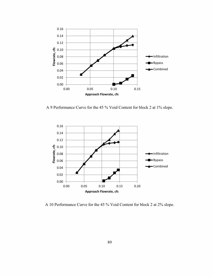
89
A 9 Performance Curve for the 45 % Void Content for block 2 at 1% slope.
A 10 Performance Curve for the 45 % Void Content for block 2 at 2% slope.
0.00
0.02
0.04
0.06
0.08
0.10
0.12
0.14
0.16
0.00 0.05 0.10 0.15
Flo
wra
te, c
fs
Approach Flowrate, cfs
Infiltration
Bypass
Combined
0.00
0.02
0.04
0.06
0.08
0.10
0.12
0.14
0.16
0.00 0.05 0.10 0.15 0.20
Flo
wra
te, c
fs
Approach Flowrate, cfs
Infiltration
Bypass
Combined

90
A 11 Performance Curve for the 45 % Void Content for block 2 at 5% slope.
A 12 Performance Curve for the 45 % Void Content for block 2 at 10% slope.
0.00
0.02
0.04
0.06
0.08
0.10
0.12
0.14
0.16
0.18
0.00 0.05 0.10 0.15 0.20
Flo
wra
te, c
fs
Approach Flowrate, cfs
Infiltration
Bypass
Combined
0.00
0.02
0.04
0.06
0.08
0.10
0.12
0.14
0.16
0.00 0.05 0.10 0.15 0.20
Flo
wra
te, c
fs
Approach Flowrate, cfs
Infiltration
Bypass
Combined

91
A 13 Performance Curve for the 45 % Void Content for block 3 at 0% slope.
A 14 Performance Curve for the 45 % Void Content for block 3 at 0.5% slope.
0.00
0.02
0.04
0.06
0.08
0.10
0.12
0.14
0.16
0.00 0.05 0.10 0.15 0.20
Flo
wra
te, c
fs
Approach Flowrate, cfs
Infiltration
Bypass
Combined
0.00
0.02
0.04
0.06
0.08
0.10
0.12
0.14
0.16
0.00 0.05 0.10 0.15 0.20
Flo
wra
te, c
fs
Approach Flowrate, cfs
Infiltration
Bypass
Combined

92
A 15 Performance Curve for the 45 % Void Content for block 3 at 1% slope.
A 16 Performance Curve for the 45 % Void Content for block 3 at 2% slope.
0.00
0.02
0.04
0.06
0.08
0.10
0.12
0.14
0.16
0.18
0.00 0.05 0.10 0.15 0.20
Flo
wra
te, c
fs
Approach Flowrate, cfs
Infiltration
Bypass
Combined
0.00
0.02
0.04
0.06
0.08
0.10
0.12
0.14
0.16
0.18
0.00 0.05 0.10 0.15 0.20
Flo
wra
te, c
fs
Approach Flowrate, cfs
Infiltration
Bypass
Combined
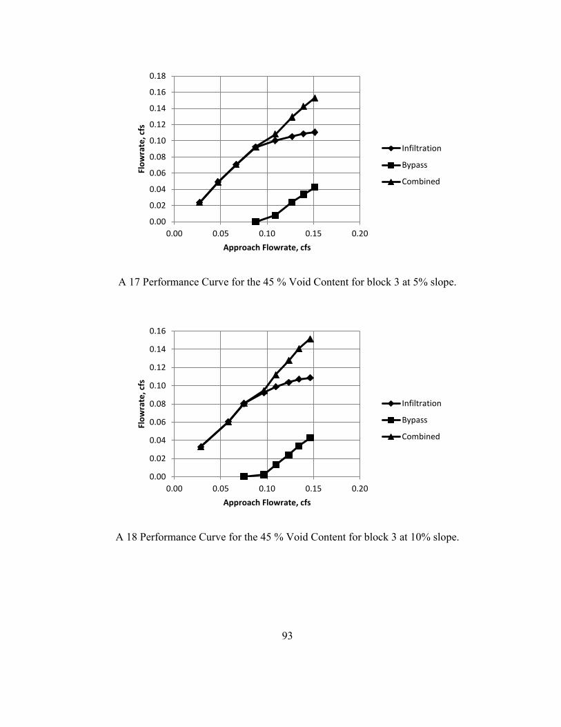
93
A 17 Performance Curve for the 45 % Void Content for block 3 at 5% slope.
A 18 Performance Curve for the 45 % Void Content for block 3 at 10% slope.
0.00
0.02
0.04
0.06
0.08
0.10
0.12
0.14
0.16
0.18
0.00 0.05 0.10 0.15 0.20
Flo
wra
te, c
fs
Approach Flowrate, cfs
Infiltration
Bypass
Combined
0.00
0.02
0.04
0.06
0.08
0.10
0.12
0.14
0.16
0.00 0.05 0.10 0.15 0.20
Flo
wra
te, c
fs
Approach Flowrate, cfs
Infiltration
Bypass
Combined

94
A 19 Performance Curve for the 35 % Void Content for block 1 at 0% slope.
A 20 Performance Curve for the 35 % Void Content for block 1 at 0.5% slope.
0.00
0.02
0.04
0.06
0.08
0.10
0.12
0.14
0.00 0.02 0.04 0.06 0.08 0.10 0.12 0.14
Flo
wra
te, c
fs
Approach Flowrate, cfs
Infiltration
Bypass
combined
0.00
0.02
0.04
0.06
0.08
0.10
0.12
0.14
0.00 0.02 0.04 0.06 0.08 0.10 0.12 0.14
Flo
wra
te, c
fs
Approach Flowrate, cfs
Infiltration
Bypass
Combined

95
A 21 Performance Curve for the 35 % Void Content for block 1 at 1% slope.
A 22 Performance Curve for the 35 % Void Content for block 1 at 2% slope.
0.00
0.02
0.04
0.06
0.08
0.10
0.12
0.14
0.00 0.02 0.04 0.06 0.08 0.10 0.12 0.14
Flo
wra
te, c
fs
Approach Flowrate, cfs
Infiltration
Bypass
combined
0.00
0.02
0.04
0.06
0.08
0.10
0.12
0.14
0.00 0.02 0.04 0.06 0.08 0.10 0.12 0.14
Flo
wra
te, c
fs
Approach Flowrate, cfs
Infiltration
Bypass
Combined
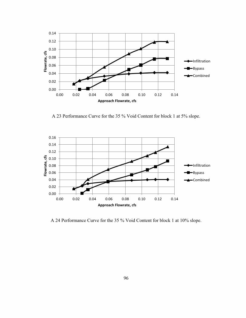
96
A 23 Performance Curve for the 35 % Void Content for block 1 at 5% slope.
A 24 Performance Curve for the 35 % Void Content for block 1 at 10% slope.
0.00
0.02
0.04
0.06
0.08
0.10
0.12
0.14
0.00 0.02 0.04 0.06 0.08 0.10 0.12 0.14
Flo
wra
te, c
fs
Approach Flowrate, cfs
Infiltration
Bypass
Combined
0.00
0.02
0.04
0.06
0.08
0.10
0.12
0.14
0.16
0.00 0.02 0.04 0.06 0.08 0.10 0.12 0.14
Flo
wra
te, c
fs
Approach Flowrate, cfs
Infiltration
Bypass
Combined

97
A 25 Performance Curve for the 35 % Void Content for block 2 at 0% slope.
A 26 Performance Curve for the 35 % Void Content for block 2 at 0.5% slope.
0.00
0.02
0.04
0.06
0.08
0.10
0.12
0.14
0.00 0.05 0.10 0.15
Flo
wra
te, c
fs
Approach Flowrate, cfs
Infiltration
Bypass
Combined
0.00
0.02
0.04
0.06
0.08
0.10
0.12
0.14
0.00 0.05 0.10 0.15
Flo
wra
te, c
fs
Approach Flowrate, cfs
Infiltration
Bypass
Combined
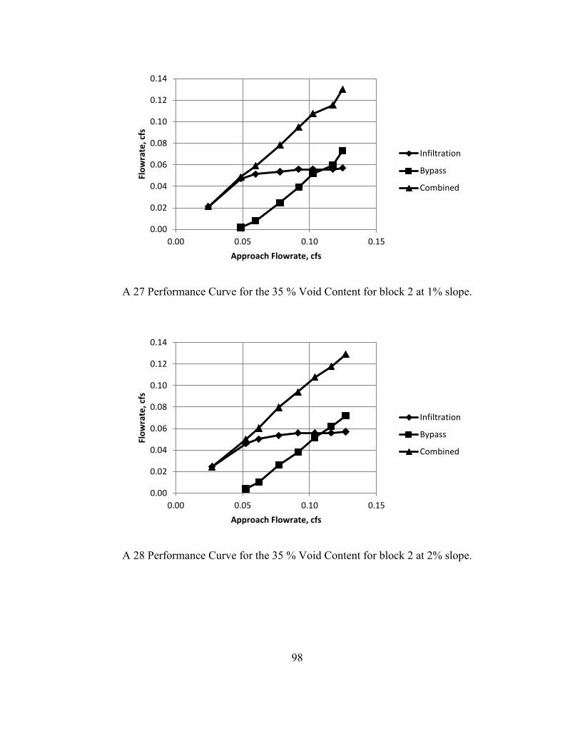
98
A 27 Performance Curve for the 35 % Void Content for block 2 at 1% slope.
A 28 Performance Curve for the 35 % Void Content for block 2 at 2% slope.
0.00
0.02
0.04
0.06
0.08
0.10
0.12
0.14
0.00 0.05 0.10 0.15
Flo
wra
te, c
fs
Approach Flowrate, cfs
Infiltration
Bypass
Combined
0.00
0.02
0.04
0.06
0.08
0.10
0.12
0.14
0.00 0.05 0.10 0.15
Flo
wra
te, c
fs
Approach Flowrate, cfs
Infiltration
Bypass
Combined

99
A 29 Performance Curve for the 35 % Void Content for block 2 at 5% slope.
A 30 Performance Curve for the 35 % Void Content for block 2 at 10% slope.
0.00
0.02
0.04
0.06
0.08
0.10
0.12
0.14
0.00 0.05 0.10 0.15
Flo
wra
te, c
fs
Approach Flowrate, cfs
Infiltration
Bypass
Combined
0.00
0.02
0.04
0.06
0.08
0.10
0.12
0.14
0.00 0.05 0.10 0.15
Flo
wra
te, c
fs
Approach Flowrate, cfs
Infiltration
Bypass
Combined

100
A 31 Performance Curve for the 35 % Void Content for block 3 at 0% slope.
A 32 Performance Curve for the 35 % Void Content for block 3 at 0.5% slope.
0.00
0.02
0.04
0.06
0.08
0.10
0.12
0.14
0.16
0.00 0.05 0.10 0.15 0.20
Flo
wra
te, c
fs
Approach Flowrate, cfs
Infiltration
Bypass
Combined
0.00
0.02
0.04
0.06
0.08
0.10
0.12
0.14
0.00 0.05 0.10 0.15
Flo
wra
te, c
fs
Approach Flowrate, cfs
Infiltration
Bypass
Combined

101
A 33 Performance Curve for the 35 % Void Content for block 3 at 1% slope.
A 34 Performance Curve for the 35 % Void Content for block 3 at 2% slope.
0.00
0.02
0.04
0.06
0.08
0.10
0.12
0.14
0.00 0.05 0.10 0.15
Flo
wra
te, c
fs
Approach Flowrate, cfs
Infiltration
Bypass
Combined
0.00
0.02
0.04
0.06
0.08
0.10
0.12
0.14
0.00 0.05 0.10 0.15
Flo
wra
te, c
fs
Approach Flowrate, cfs
Infiltration
Bypass
Combined

102
A 35 Performance Curve for the 35 % Void Content for block 3 at 5% slope.
A 36 Performance Curve for the 35 % Void Content for block 3 at 10% slope.
0.00
0.02
0.04
0.06
0.08
0.10
0.12
0.14
0.00 0.05 0.10 0.15
Flo
wra
te, c
fs
Approach Flowrate, cfs
Infiltration
Bypass
Combined
0.00
0.02
0.04
0.06
0.08
0.10
0.12
0.14
0.00 0.05 0.10 0.15
Flo
wra
te, c
fs
Approach Flowrate, cfs
Infiltration
Bypass
Combined

103
A 37 Performance Curve for the 20 % Void Content for block 1 at 0% slope.
A 38 Performance Curve for the 20 % Void Content for block 1 at 0.5% slope.
0.00
0.02
0.04
0.06
0.08
0.10
0.12
0.00 0.02 0.04 0.06 0.08 0.10 0.12
Flo
wra
te, c
fs
Approach Flowrate, cfs
Infiltration
Bypass
combined
0.00
0.02
0.04
0.06
0.08
0.10
0.12
0.00 0.02 0.04 0.06 0.08 0.10
Flo
wra
te, c
fs
Approach Flowrate, cfs
Infiltration
Bypass
combined

104
A 39 Performance Curve for the 20 % Void Content for block 1 at 1% slope.
A 40 Performance Curve for the 20 % Void Content for block 1 at 2% slope.
0.00
0.02
0.04
0.06
0.08
0.10
0.12
0.00 0.02 0.04 0.06 0.08 0.10 0.12
Flo
wra
te, c
fs
Approach Flowrate, cfs
Infiltration
Bypass
combined
0.00
0.02
0.04
0.06
0.08
0.10
0.12
0.00 0.02 0.04 0.06 0.08 0.10
Flo
wra
te, c
fs
Approach Flowrate, cfs
Infiltration
Bypass
combined

105
A 41 Performance Curve for the 20 % Void Content for block 1 at 5% slope.
A 42 Performance Curve for the 20 % Void Content for block 1 at 10% slope.
0.00
0.02
0.04
0.06
0.08
0.10
0.12
0.00 0.02 0.04 0.06 0.08 0.10 0.12
Flo
wra
te, c
fs
Approach Flowrate, cfs
Infiltration
Bypass
combined
0.00
0.02
0.04
0.06
0.08
0.10
0.12
0.00 0.02 0.04 0.06 0.08 0.10 0.12
Flo
wra
te, c
fs
Approach Flowrate, cfs
Infiltration
Bypass
combined

106
A 43 Performance Curve for the 20 % Void Content for block 2 at 0% slope.
A 44 Performance Curve for the 20 % Void Content for block 2 at 0.5% slope.
0.00
0.01
0.02
0.03
0.04
0.05
0.06
0.07
0.08
0.09
0.10
0.00 0.02 0.04 0.06 0.08 0.10
Flo
wra
te, c
fs
Approach Flowrate, cfs
Infiltration
Bypass
Combined
0.00
0.02
0.04
0.06
0.08
0.10
0.12
0.00 0.02 0.04 0.06 0.08 0.10
Flo
wra
te, c
fs
Approach Flowrate, cfs
Infiltration
Bypass
Combined

107
A 45 Performance Curve for the 20 % Void Content for block 2 at 1% slope.
A 46 Performance Curve for the 20 % Void Content for block 2 at 2% slope.
0.00
0.02
0.04
0.06
0.08
0.10
0.12
0.00 0.02 0.04 0.06 0.08 0.10
Flo
wra
te, c
fs
Approach Flowrate, cfs
Infiltration
Bypass
Combined
0.00
0.01
0.02
0.03
0.04
0.05
0.06
0.07
0.08
0.09
0.10
0.00 0.02 0.04 0.06 0.08 0.10
Flo
wra
te, c
fs
Approach Flowrate, cfs
Infiltration
Bypass
Combined

108
A 47 Performance Curve for the 20 % Void Content for block 2 at 5% slope.
A 48 Performance Curve for the 20 % Void Content for block 2 at 10% slope.
0.00
0.02
0.04
0.06
0.08
0.10
0.12
0.00 0.02 0.04 0.06 0.08 0.10
Flo
wra
te, c
fs
Approach Flowrate, cfs
Infiltration
Bypass
Combined
0.00
0.01
0.02
0.03
0.04
0.05
0.06
0.07
0.08
0.09
0.10
0.00 0.02 0.04 0.06 0.08 0.10
Flo
wra
te, c
fs
Approach Flowrate, cfs
Infiltration
Bypass
Combined

109
A 49 Performance Curve for the 20 % Void Content for block 3 at 0% slope.
A 50 Performance Curve for the 20 % Void Content for block 3 at 0.5% slope.
0.00
0.01
0.02
0.03
0.04
0.05
0.06
0.07
0.08
0.09
0.10
0.00 0.02 0.04 0.06 0.08 0.10
Flo
wra
te, c
fs
Approach Flowrate, cfs
Infiltration
Bypass
Combined
0.00
0.01
0.02
0.03
0.04
0.05
0.06
0.07
0.08
0.09
0.10
0.00 0.02 0.04 0.06 0.08 0.10
Flo
wra
te, c
fs
Approach Flowrate, cfs
Infiltration
Bypass
Combined
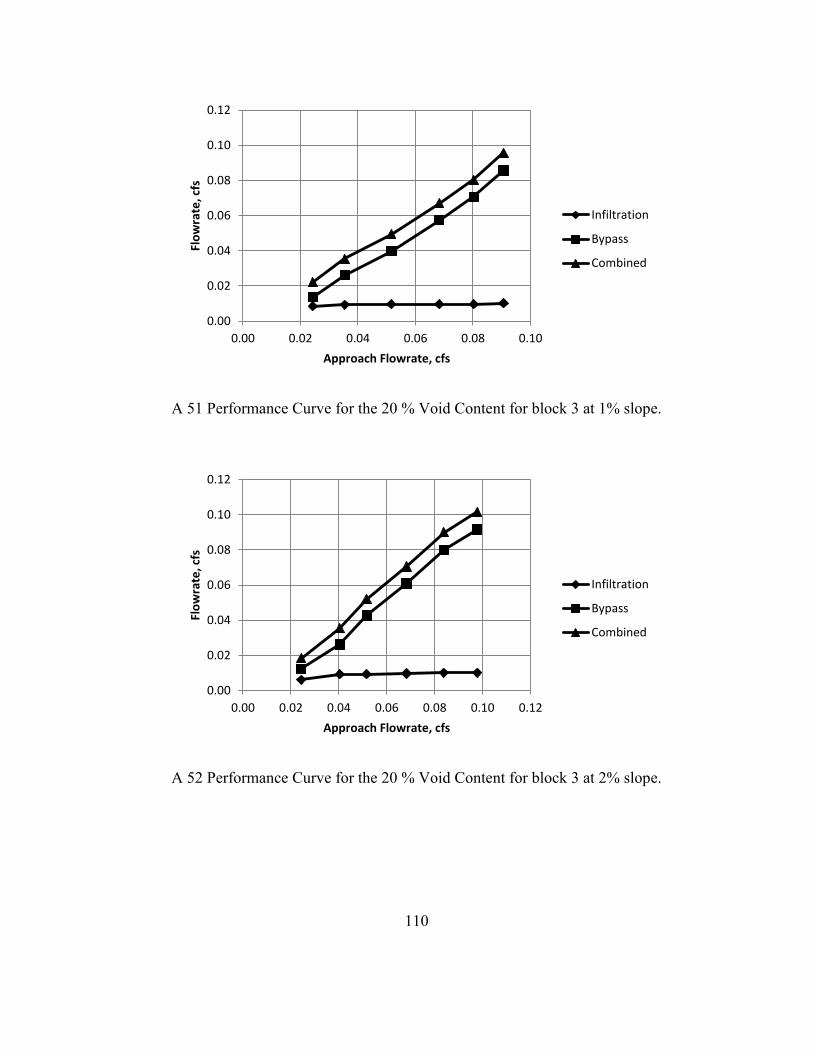
110
A 51 Performance Curve for the 20 % Void Content for block 3 at 1% slope.
A 52 Performance Curve for the 20 % Void Content for block 3 at 2% slope.
0.00
0.02
0.04
0.06
0.08
0.10
0.12
0.00 0.02 0.04 0.06 0.08 0.10
Flo
wra
te, c
fs
Approach Flowrate, cfs
Infiltration
Bypass
Combined
0.00
0.02
0.04
0.06
0.08
0.10
0.12
0.00 0.02 0.04 0.06 0.08 0.10 0.12
Flo
wra
te, c
fs
Approach Flowrate, cfs
Infiltration
Bypass
Combined
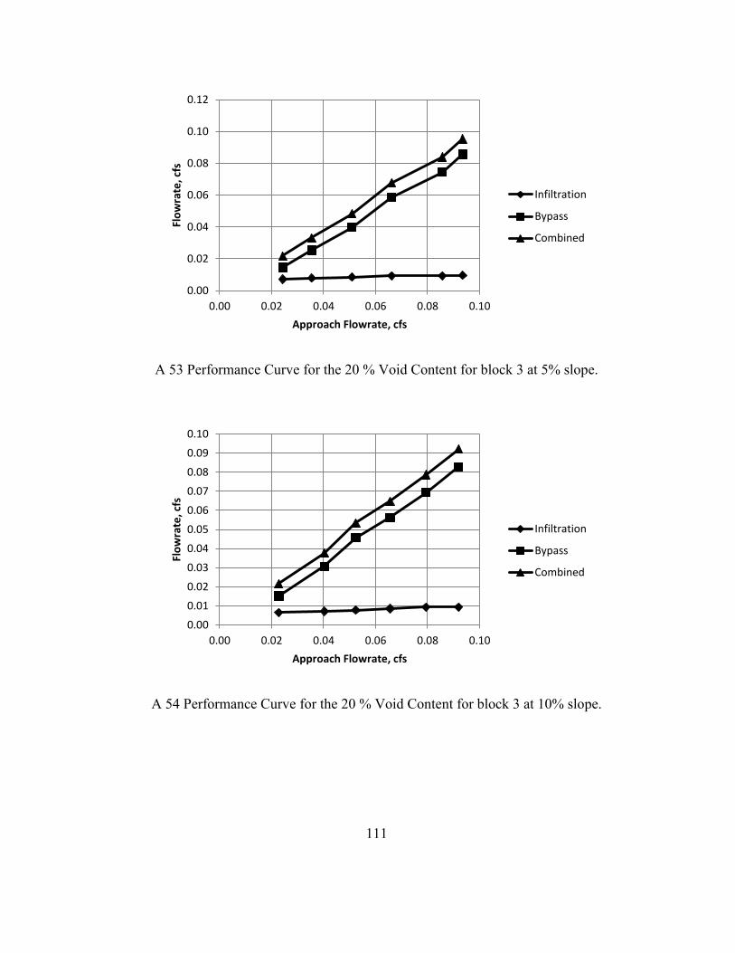
111
A 53 Performance Curve for the 20 % Void Content for block 3 at 5% slope.
A 54 Performance Curve for the 20 % Void Content for block 3 at 10% slope.
0.00
0.02
0.04
0.06
0.08
0.10
0.12
0.00 0.02 0.04 0.06 0.08 0.10
Flo
wra
te, c
fs
Approach Flowrate, cfs
Infiltration
Bypass
Combined
0.00
0.01
0.02
0.03
0.04
0.05
0.06
0.07
0.08
0.09
0.10
0.00 0.02 0.04 0.06 0.08 0.10
Flo
wra
te, c
fs
Approach Flowrate, cfs
Infiltration
Bypass
Combined

112
A 55 Performance Curve for the 25 % Void Content for block 1 at 0% slope.
A 56 Performance Curve for the 25 % Void Content for block 1 at 0.5% slope.
0.00
0.01
0.02
0.03
0.04
0.05
0.06
0.07
0.08
0.09
0.10
0.00 0.02 0.04 0.06 0.08 0.10
Flo
wra
te, c
fs
Approach Flowrate, cfs
Infiltration
Bypass
Combined
0.00
0.01
0.02
0.03
0.04
0.05
0.06
0.07
0.08
0.09
0.10
0.00 0.02 0.04 0.06 0.08 0.10
Flo
wra
te, c
fs
Approach Flowrate, cfs
Infiltration
Bypass
Combined

113
A 57 Performance Curve for the 25 % Void Content for block 1 at 1% slope.
A 58 Performance Curve for the 25 % Void Content for block 1 at 2% slope.
0.00
0.01
0.02
0.03
0.04
0.05
0.06
0.07
0.08
0.09
0.00 0.02 0.04 0.06 0.08 0.10
Flo
wra
te, c
fs
Approach Flowrate, cfs
Infiltration
Bypass
Combined
0.00
0.01
0.02
0.03
0.04
0.05
0.06
0.07
0.08
0.09
0.10
0.00 0.02 0.04 0.06 0.08 0.10
Flo
wra
te, c
fs
Approach Flowrate, cfs
Infiltration
Bypass
Combined

114
A 59 Performance Curve for the 25 % Void Content for block 1 at 5% slope.
A 60 Performance Curve for the 25 % Void Content for block 1 at 10% slope.
0.00
0.01
0.02
0.03
0.04
0.05
0.06
0.07
0.08
0.09
0.00 0.02 0.04 0.06 0.08 0.10
Flo
wra
te, c
fs
Approach Flowrate, cfs
Infiltration
Bypass
Combined
0.00
0.01
0.02
0.03
0.04
0.05
0.06
0.07
0.08
0.09
0.00 0.02 0.04 0.06 0.08 0.10
Flo
wra
te, c
fs
Approach Flowrate, cfs
Infiltration
Bypass
Combined

115
A 61 Performance Curve for the 25 % Void Content for block 2 at 0% slope.
A 62 Performance Curve for the 25 % Void Content for block 2 at 0.5% slope.
0.00
0.01
0.02
0.03
0.04
0.05
0.06
0.07
0.08
0.09
0.10
0.00 0.02 0.04 0.06 0.08 0.10 0.12
Flo
wra
te, c
fs
Approach Flowrate, cfs
Infiltration
Bypass
Combined
0.00
0.02
0.04
0.06
0.08
0.10
0.12
0.00 0.02 0.04 0.06 0.08 0.10 0.12
Flo
wra
te, c
fs
Approach Flowrate, cfs
Infiltration
Bypass
Combined

116
A 63 Performance Curve for the 25 % Void Content for block 2 at 1% slope.
A 64 Performance Curve for the 25 % Void Content for block 2 at 2% slope.
0.00
0.02
0.04
0.06
0.08
0.10
0.12
0.00 0.02 0.04 0.06 0.08 0.10 0.12
Flo
wra
te, c
fs
Approach Flowrate, cfs
Infiltration
Bypass
Combined
0.00
0.02
0.04
0.06
0.08
0.10
0.12
0.00 0.02 0.04 0.06 0.08 0.10 0.12
Flo
wra
te, c
fs
Approach Flowrate, cfs
Infiltration
Bypass
Combined

117
A 65 Performance Curve for the 25 % Void Content for block 2 at 5% slope.
A 66 Performance Curve for the 25 % Void Content for block 2 at 10% slope.
0.00
0.02
0.04
0.06
0.08
0.10
0.12
0.00 0.02 0.04 0.06 0.08 0.10
Flo
wra
te, c
fs
Approach Flowrate, cfs
Infiltration
Bypass
Combined
0.00
0.01
0.02
0.03
0.04
0.05
0.06
0.07
0.08
0.09
0.10
0.00 0.02 0.04 0.06 0.08 0.10
Flo
wra
te, c
fs
Approach Flowrate, cfs
Infiltration
Bypass
Combined

118
A 67 Performance Curve for the 25 % Void Content for block 3 at 0% slope.
A 68 Performance Curve for the 25 % Void Content for block 3 at 0.5% slope.
0.00
0.01
0.02
0.03
0.04
0.05
0.06
0.07
0.08
0.09
0.00 0.02 0.04 0.06 0.08 0.10
Flo
wra
te, c
fs
Approach Flowrate, cfs
Infiltration
Bypass
Combined
0.00
0.01
0.02
0.03
0.04
0.05
0.06
0.07
0.08
0.09
0.00 0.02 0.04 0.06 0.08 0.10
Flo
wra
te, c
fs
Approach Flowrate, cfs
Infiltration
Bypass
Combined

119
A 69 Performance Curve for the 25 % Void Content for block 3 at 1% slope.
A 70 Performance Curve for the 25 % Void Content for block 3 at 2% slope.
0.00
0.01
0.02
0.03
0.04
0.05
0.06
0.07
0.08
0.09
0.00 0.02 0.04 0.06 0.08 0.10
Flo
wra
te, c
fs
Approach Flowrate, cfs
Infiltration
Bypass
Combined
0.00
0.01
0.02
0.03
0.04
0.05
0.06
0.07
0.08
0.00 0.02 0.04 0.06 0.08 0.10
Flo
wra
te, c
fs
Approach Flowrate, cfs
Infiltration
Bypass
Combined

120
A 71 Performance Curve for the 25 % Void Content for block 3 at 5% slope.
A 72 Performance Curve for the 25 % Void Content for block 3 at 10% slope.
0.00
0.01
0.02
0.03
0.04
0.05
0.06
0.07
0.08
0.09
0.00 0.02 0.04 0.06 0.08 0.10
Flo
wra
te, c
fs
Approach Flowrate, cfs
Infiltration
Bypass
Combined
0.00
0.01
0.02
0.03
0.04
0.05
0.06
0.07
0.08
0.00 0.02 0.04 0.06 0.08 0.10
Flo
wra
te, c
fs
Approach Flowrate, cfs
Infiltration
Bypass
Combined

121
A 73 Performance Curve for the 15 % Void Content for block 1 at 0% slope.
A 74 Performance Curve for the 15 % Void Content for block 1 at 0.5% slope.
0.00
0.01
0.02
0.03
0.04
0.05
0.06
0.07
0.08
0.09
0.10
0.00 0.02 0.04 0.06 0.08 0.10
Flo
wra
te, c
fs
Approach Flowrate, cfs
Infiltration
Bypass
Combined
0.00
0.01
0.02
0.03
0.04
0.05
0.06
0.07
0.08
0.09
0.10
0.00 0.02 0.04 0.06 0.08 0.10
Flo
wra
te, c
fs
Approach Flowrate, cfs
Infiltration
Bypass
Combined

122
A 75 Performance Curve for the 15 % Void Content for block 1 at 1% slope.
A 76 Performance Curve for the 15 % Void Content for block 1 at 2% slope.
0.00
0.01
0.02
0.03
0.04
0.05
0.06
0.07
0.08
0.09
0.10
0.00 0.02 0.04 0.06 0.08 0.10
Flo
wra
te, c
fs
Approach Flowrate, cfs
Infiltration
Bypass
Combined
0.00
0.01
0.02
0.03
0.04
0.05
0.06
0.07
0.08
0.09
0.10
0.00 0.02 0.04 0.06 0.08 0.10
Flo
wra
te, c
fs
Approach Flowrate, cfs
Infiltration
Bypass
Combined

123
A 77 Performance Curve for the 15 % Void Content for block 1 at 5% slope.
A 78 Performance Curve for the 15 % Void Content for block 1 at 10% slope.
0.00
0.01
0.02
0.03
0.04
0.05
0.06
0.07
0.08
0.09
0.10
0.00 0.02 0.04 0.06 0.08 0.10
Flo
wra
te, c
fs
Approach Flowrate, cfs
Infiltration
Bypass
Combined
0.00
0.01
0.02
0.03
0.04
0.05
0.06
0.07
0.08
0.09
0.10
0.00 0.02 0.04 0.06 0.08 0.10
Flo
wra
te, c
fs
Approach Flowrate, cfs
Infiltration
Bypass
Combined

124
A 79 Performance Curve for the 15 % Void Content for block 2 at 0% slope.
A 80 Performance Curve for the 15 % Void Content for block 2 at 0.5% slope.
0.00
0.01
0.02
0.03
0.04
0.05
0.06
0.07
0.08
0.09
0.00 0.02 0.04 0.06 0.08 0.10
Flo
wra
te, c
fs
Approach Flowrate, cfs
Infiltration
Bypass
Combined
0.00
0.01
0.02
0.03
0.04
0.05
0.06
0.07
0.08
0.09
0.00 0.02 0.04 0.06 0.08 0.10
Flo
wra
te, c
fs
Approach Flowrate, cfs
Infiltration
Bypass
Combined

125
A 81 Performance Curve for the 15 % Void Content for block 2 at 1% slope.
A 82 Performance Curve for the 15 % Void Content for block 2 at 2% slope.
0.00
0.01
0.02
0.03
0.04
0.05
0.06
0.07
0.08
0.09
0.10
0.00 0.02 0.04 0.06 0.08 0.10
Flo
wra
te, c
fs
Approach Flowrate, cfs
Infiltration
Bypass
Combined
0.00
0.01
0.02
0.03
0.04
0.05
0.06
0.07
0.08
0.09
0.00 0.02 0.04 0.06 0.08 0.10
Flo
wra
te, c
fs
Approach Flowrate, cfs
Infiltration
Bypass
Combined

126
A 83 Performance Curve for the 15 % Void Content for block 2 at 5% slope.
A 84 Performance Curve for the 15 % Void Content for block 2 at 10% slope.
0.00
0.01
0.02
0.03
0.04
0.05
0.06
0.07
0.08
0.09
0.00 0.02 0.04 0.06 0.08 0.10
Flo
wra
te, c
fs
Approach Flowrate, cfs
Infiltration
Bypass
Combined
0.00
0.01
0.02
0.03
0.04
0.05
0.06
0.07
0.08
0.09
0.10
0.00 0.02 0.04 0.06 0.08 0.10
Flo
wra
te, c
fs
Approach Flowrate, cfs
Infiltration
Bypass
Combined

127
A 85 Performance Curve for the 15 % Void Content for block 3 at 0% slope.
A 86 Performance Curve for the 15 % Void Content for block 3 at 0.5% slope.
0.00
0.01
0.02
0.03
0.04
0.05
0.06
0.07
0.08
0.09
0.00 0.02 0.04 0.06 0.08 0.10
Flo
wra
te, c
fs
Approach Flowrate, cfs
Infiltration
Bypass
Combined
0.00
0.01
0.02
0.03
0.04
0.05
0.06
0.07
0.08
0.09
0.00 0.02 0.04 0.06 0.08 0.10
Flo
wra
te, c
fs
Approach Flowrate, cfs
Infiltration
Bypass
Combined
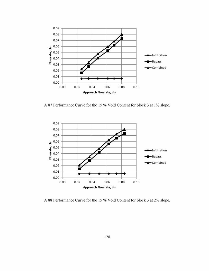
128
A 87 Performance Curve for the 15 % Void Content for block 3 at 1% slope.
A 88 Performance Curve for the 15 % Void Content for block 3 at 2% slope.
0.00
0.01
0.02
0.03
0.04
0.05
0.06
0.07
0.08
0.09
0.00 0.02 0.04 0.06 0.08 0.10
Flo
wra
te, c
fs
Approach Flowrate, cfs
Infiltration
Bypass
Combined
0.00
0.01
0.02
0.03
0.04
0.05
0.06
0.07
0.08
0.09
0.00 0.02 0.04 0.06 0.08 0.10
Flo
wra
te, c
fs
Approach Flowrate, cfs
Infiltration
Bypass
Combined

129
A 89 Performance Curve for the 15 % Void Content for block 3 at 5% slope.
A 90 Performance Curve for the 15 % Void Content for block 3 at 10% slope.
0.00
0.01
0.02
0.03
0.04
0.05
0.06
0.07
0.08
0.09
0.10
0.00 0.02 0.04 0.06 0.08 0.10
Flo
wra
te, c
fs
Approach Flowrate, cfs
Infiltration
Bypass
Combined
0.00
0.01
0.02
0.03
0.04
0.05
0.06
0.07
0.08
0.09
0.00 0.02 0.04 0.06 0.08 0.10
Flo
wra
te, c
fs
Approach Flowrate, cfs
Infiltration
Bypass
Combined

130
VITA
Nathan Andrew Grahl was born on April 15th
1988 in Independence Missouri. He
attended Archbishop O’Hara High School in Kansas City Missouri. He then studied pre-
Engineering at Northwest Missouri State University before completing his Bachelors of
Science in Civil Engineering from the University of Missouri- Kansas City. While at the
University of Missouri- Kansas City Nathan became active in student organizations and
became an officer in the following student organizations: Chi epsilon, Design Build
Institute of America, and the American Concrete Institute. Nathan worked for several years
in the labs at UMKC performing research for Dr. John Kevern and currently works for
Black & Veatch in the Water Division at the office in Kansas City Missouri.