Hydraulic jumps at boundaries in rotating fluids · with the jump amplitude as the small parameter, applied both to the wave field behind the jump and to the matching conditions

J Fluid Mech (IYYh), rol 324. p p 55-82 Copyright 0 1996 Cambridge Universit! Press

55

Hydraulic jumps at boundaries in rotating fluids By ALEXEY V. F E D O R O V A N D W. K E N D A L L MELVILLE

Scripps Institution of Oceanography, University of California San Diego, La Jolla, CA 92093-0213, USA

(Received 20 October 1994 and in revised form 2 January 1996)

We consider three-dimensional hydraulic jumps (shocks) propagating along boundaries in rotating fluids. This study is motivated by earlier work (Fedorov & Melville 1995), which dealt with the evolution to breaking of nonlinear Kelvin waves. We obtain the jump relations and derive an evolution equation for the jump as it propagates along the boundary. It is shown that after some initial adjustment the Kelvin-type jump assumes a permanent form and propagates with a constant velocity along the boundary or the coast. At some distance offshore the jump becomes oblique to the coastline, and the final shape of the jump and its speed depend only on the jump strength. The jump gives rise to a moderate mass transport offshore. The potential vorticity remains almost constant across the jump. The energy loss in the jump is proportional to the third power of the jump amplitude, which is similar to classical two-dimensional hydraulic jumps in non-rotating fluids. Jump properties are discussed for both weak and strong nonlinearity, and the role of a boundary layer region behind the leading edge of the jump is considered.

1. Introduction In this paper we study internal hydraulic jumps (or shocks), with a transverse

structure similar to that of a Kelvin wave. Such shocks can be induced by a rapid elevation of the isopycnals over a large area adjacent to the coast, which may result from either a storm crossing the coastline (Welander 1961), or a flood increasing fresh water influx from a river plume (Garvine 1987). A steady hydraulic jump may also be established when a coastal current is incident on topography (Pratt 1983, 1987). Similar phenomena may occur in meteorology (Parret & Cullen 1984). Along the western coast of North America the predominant northerly winds may experience relaxation or even abrupt reversal (Beardsley et ul. 1987; Mass & Albright 1987). Similar wind events are observed along the coast of Australia (Baines 1980) and southern Africa (Gill 1977; Bannon 1981). There are indications that these phenomena may be associated with hydraulic jumps travelling in the atmospheric marine layer adjacent to coastal mountain ranges (Dorman 1987; Hermann et a/ . 1990).

The propagation of such jumps, and especially internal-wave jumps in coastal areas, will be affected by rotation, as long as the width of the affected region is comparable to the baroclinic Rossby radius of deformation (about 5-50 km in the ocean, and 5&200 km in the atmosphere). While hydraulic jumps in rivers and straits are well- studied (Stoker 1958; Chow 1959; Lighthill 1978; also Armi & Farmer 1985; Armi 1986). there are still many uncertainties associated with hydraulic jumps in rotating fluids. Different authors have included rotation in shock descriptions, but most assumed that the jump dynamics were essentially two-dimensional (Houghton 1969 ; Bennett & Cummins 1988 ; O’Donnell 1989). Starting from the three-dimensional problem, Stern (1980) assumed piecewise-uniform potential vorticity flow and

56 A . V. Fedorov and W. K. Melville

integrated the equations of motion with respect to the cross-flow coordinate, thereby avoiding consideration of the transverse structure of the flow. Nevertheless, during the last decade work on true three-dimensional hydraulic jumps has progressed (Pratt 1983, 1987; Nof 1984, 1986).

In his early model, Nof (1984) did not specify the profile of the jump in space, nor did he assume that the area occupied by the flow exceeded the Rossby radius of deformation. The flow in which the jump was established was unidirectional and did not depend upon the transverse coordinate. A principal assumption of the model was the conservation of potential vorticity across the shock. In another model, Nof (1986) represented the jump by a straight line normal to the coast. This would remain a good approximation for the jump propagation in a channel of width significantly smaller than the Rossby radius. In this latter work he concluded that the vorticity was not necessarily conserved across the shock.

All of these two- and three-dimensional studies demonstrate that jumps or shocks may exist in rotating fluids, and, for the present study, the numerical and experimental work of Pratt (1983, 1987) is most relevant. In particular, Pratt shows that the jump amplitude may decay offshore in a manner similar to a Kelvin wave, and that the jump becomes oblique to the coastline at some distance offshore. As will be shown below, with the assumption of exponential decay of the wave amplitude behind the shock, our analysis yields the value of that oblique angle offshore. Instead of a channel flow, we consider a semi-infinite ocean, but the problem remains similar to the channel problem studied by Pratt.

Another basis for our analysis is the work by Bennet (1973) and Fedorov & Melville (1995), who showed that the breaking of non-dispersive internal Kelvin waves was analogous to regular hyperbolic breaking. Therefore, we expect that Kelvin hydraulic jumps will retain some similarity to hydraulic jumps in the absence of rotation, which are associated with wave breaking and turbulent dissipation. Here we use the long- wave assumption, so that we can neglect dispersion, which is important for coastally trapped waves on shorter scales (Tomasson & Melville 1992; Renouard, Tomasson & Melville 1992).

We consider a coastal current entering still water, giving rise to a Kelvin jump. The problem is similar to that of a jump due to an abrupt change of velocity in a coastal current. In our model the jump is the boundary between the still water and the area with (to leading order) a geostrophic current. The equation of motion for this boundary is derived. In a simplified formulation, the problem is reduced to a forced nonlinear equation of the form

Pt + PPy = e-”, which has steady wave solutions, corresponding to a translation of the jump at a constant speed. The initial value problem for (1.1) is solved by the method of characteristics.

The structure of the paper is as follows. In $32 and 3 we consider a simplified method to obtain the evolution of the jump for weak nonlinearity. This method is based on a straightforward integration of the shallow-water equations across the jump with an extra assumption of a weak transverse velocity field. The simplified model does not satisfy the boundary conditions on the transverse velocity, nor can it describe the alongshore changes in the wave field behind the jump. That is why in $64 and 5 we consider a more complicated scheme, which is based on a singular perturbation analysis and gives an accurate mathematical solution of the problem, including an internal boundary layer in the lee of the jump. Comparing the latter solution with the simplified solution shows that the simplified version still describes the shape of the

Hydmulic ,jurnps ut boundaries in rotating fluids 57

A B

I I,,, ////////////%/I/I///“‘. m .Y FIGURE 1. Plan view of a coastal ocean with a hydraulic jump propagating to the right.

The fluid in region B is at rest.

jump very well. Consequently, in $6 we find it useful to solve the initial value problem for both models. In 937 and 8 we extend the simplified model to the case of strong nonlinearity and argue that it may still give a good qualitative description of the phenomenon, as long as the transverse velocity remains relatively small.

The improved model for the weakly nonlinear case represents an expansion scheme with the jump amplitude as the small parameter, applied both to the wave field behind the jump and to the matching conditions. Provided this scheme converges, the improved model yields a mathematically correct solution of the problem of a hydraulic jump in a semi-infinite rotating ocean. It gives the wave and velocity fields behind the jump, including any offshore flow. In this sense, the improved model is the central part of our work. The simple model lacks this completeness owing to neglect of one of the conditions on the offshore velocity when calculating the wave field behind the jump. So too does the strongly nonlinear theory. Nevertheless, simplified theories for both weak and strong nonlinearity appear promising for applications.

Note that for weak nonlinearity the integration of the shallow-water equations across the jump gives the same result as the integration of the equations of momentum conservation if higher-order terms are neglected. That is, the matching conditions, and consequently the equation for the jump evolution, turn out to be equivalent to leading order for both approaches. This is true only for the weakly nonlinear case, while one must use the momentum-conserving equations to obtain the matching conditions for the case of strong nonlinearity.

2. The equations of jump propagation: simplified model, weak nonlinearity

The method we apply here is similar to the conventional approach for hydraulic jumps (Lighthill 1978; Bennett & Cummins 1988), but with important variations due to three-dimensional and rotational effects. In this section we consider the case of weak nonlinearity for which we apply the non-dimensionalized shallow-water equations (Pedlosky 1987, p. 88):

u, + cL(uuz + vu,) + ‘I* - 2’ = 0, (2.1) rt + a(uu, + w,) + 7yu + u = 0, (2.2)

9t + u, + uy + duq), + &v&/ = 0, (2.3)

where x is the alongshore coordinate, y is the coordinate normai to the coastline and 4, u and v are, respectively, the elevation of a free surface, and the alongshore and


offshore velocities. The Rossby radius of deformation is equal to unity, while the nonlinearity parameter a (Rossby number) is relatively small. While the main applications of the theory are to two-layer models of oceans or atmospheres, for simplicity, we use the equations for a one-layer fluid. The one-layer model retains the essential physics, and, with an error of U(a2) , is asymptotically equivalent to the two- layer case (cf. Tomasson 1991).

We assume that variables 3, u and u have a discontinuity of finite amplitude at the jump, which occurs along a line x = R(y, t ) separating two regions (A and B) in which the variables are continuous (figure 1). The function R(y,t) then determines the position of the jump in space and time. Integrating (2.1)-(2.3) with respect to x from R--E to R+-E and taking the limit as c goes to zero gives three equations for the jump amplitudes in 7, u and v and its position R :

R+O

I R - 0 - R,[u] + $ 4 u 2 ] + [v] = - 01

- R,[v] - R, f 0 1 [ ~ ' ] - R,[ q] = - tl U V , dx,

- R, [TI + [UI - R,bI + .[u3l- aRy [ q l = 0,

U U , dx, (2.4)

(2.5)

(2.6) 1::

where

stand for the changes in the wave height and velocities across the jump, and depend upon time and the y-coordinate. Note that the integration method is different from that used by Pratt (1983) and Nof (1984), who integrated the equations of momentum flux conservation. (We use this approach for the strongly nonlinear case in $7). For weak nonlinearity, the integration of the shallow-water equations is asymptotically equivalent to the integration of the equations in the form of momentum conservation, if we neglect higher-order terms in a. Another difference is that both Pratt and Nof integrated along the direction normal to the jump line at each point of the jump.

Assuming that there is no motion in area B, one can rewrite (2.4)-(2.6) as

- R, U, + &u; + 3, = 01

- R, U , - R, &I; - R, 7, = 01

U U ~ dx, (2-8)

(2.9)

(2.10)

l.: U V , dx, 1::

- R, v,, + u,, - R, U, + CIU, 9, -aR, U , 7, = 0, where vo,u, and u, correspond to the wave field behind the jump (e.g. u, = U I , = ~ - ~ ) .

Now in order to proceed, we need to impose an additional constraint on the scales of the terms in (2.8)-(2.10). We assume that

u = U(a1"), (2.11)

which means that the offshore flow is not very strong. The small parameter in the following expansion will be a'". With the scaling (2.1 l), one can show that the terms on the right-hand side in (2.8)-(2.9) are not larger than U(a2) and 0(01~'~), respectively. Omitting these and other terms of similar and higher order yields

(2.12) (2.13)

and (2.14)

Hydraulic jurnps at boundaries in rotating fluids 59

Equation (2.12) then gives R, = 1 +O(a), (2.15)

i.e. all disturbances travel with a speed close to the speed of long gravity waves. From (2.13) i t follows now that

R , = O(al"). (2.16) Introducing r , which is the perturbation of the x-position of the jump in the frame

of reference moving at the speed of long gravity waves, we set R = t+r, (2.17)

so that R, = 1 +v, and R , = r V , (2.18) and t i , - u,, = rt u , -+xu,',. (2.19)

c, = -rz/ j ] ( p (2.20) (2.21) u, - vo = rt I , + r y ", - xu, ' l o .

From (2.19)-(2.21) we find that and adding (2.19) and (2.21). u, = 'lo + O(aL (2.22)

- 2r, + (Q +;a?/(, = 0. (2.23)

To find vie we assume that, to leading order, the wave field behind the shock

U t + r l r = 0, (2.24) 'I2/ + u = 0, (2.25) ' / t+u , = 0. (2.26)

This is an equation describing the evolution of the jump in space and time.

corresponds to a Kelvin wave; that is, (2.1)-(2.3) reduce to

Among the solutions of this system, we choose the simplest. which satisfies (2.22): u = r/ = ecy. (2.27)

This degenerate solution is a geostrophic current with the velocity decaying exponentially offshore. Substituting (2.27) into (2.23) gives an equation for the shock propagation,

2r, - r 2 Y = $a e-y, (2.28) for which the boundary condition simply follows from (2.20) and the no-flow condition at the coast:

r?/Iu=,, = 0. (2.29) Introducing p = - ry, (2.30) reduces (2.28) and (2.29) to

p, + ppu = $a cY. (2.3 1) with Ply=" = 0. (2.32) Solving (2.31)-(2.32) with an appropriate initial condition will give the evolution of the jump in space. As for the Kelvin wave, a jump with the wave field exponentially decaying offshore behind it can travel only in one direction (with the coast to the right in the Northern Hemisphere).

3. Steady wave solution for the jump: simplified model, weak nonlinearity We consider steady wave solutions of (2.28), which corresponds to the case of a

hydraulic jump simply translating along the coast. Letting Y, = .r, so that the speed of the jump relative to the coast is 1 +s, allows us to integrate (2.28). The value of s is determined immediately from the boundary condition

s = :a. (3.1)


\ I 1

Distance alongshore, x

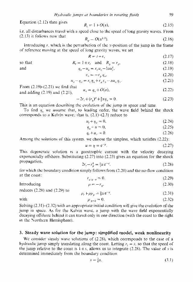
FIGURE 2. The shape of a stationary Kelvin jump travelling along the coast. Described by r = r(y , L), for cc = 0.3 (see (3.3)).

Whence, ry = -[:a( 1 - e ~ u ) ] ~ ’ ~

or (3.3)

where q = (1 -e-Y)1/2. (3.4)

The stationary jump is shown in figure 2. One of the characteristic features of this solution is that offshore it tends to an oblique angle q5 between the jump and the normal to the coast, where

fj z (;a)”2. (3.5)

A similar oblique angle was observed in experiments by Pratt (1987). He concluded that the angle depended upon the rotation speed, which is contrary to our result that the angle depends only on the strength of the jump. This contradiction may be attributed to the fact that in Pratt’s experiments the jump strength varied with the rotation speed, as can be seen from figure 4 of this paper.

4. Steady wave solution for the jump: improved model, weak nonlinearity Although we expect that the Kelvin shock solution considered in the previous

sections provides a good approximation to the shape and evolution of the jump, it has certain restrictions, especially with regard to the transverse velocity. Strictly speaking, the Kelvin-wave solution we use in the evolution equation (2.23) has zero transverse velocity, while the jump condition (2.20) implies non-zero u. One might try to resolve this in a straightforward way adding a small perturbation to the Kelvin wave, which would account for non-zero v. However, in this case the amplitude of the perturbation turns out to be comparable to the amplitude of the wave itself. The way to cope with

Hjrlvuulic jumps at hozindavies in rotating fluids 61

the problem IS to introduce a boundary layer behind the jump, with non-zero transverse velocity being confined to the boundary layer.

For simplicity, we first limit our attention to steady wave solutions, with the jump translating at a constant speed 1 +s, where s = O(s). We introduce

.f = .y-t-sst, (4.1)

(4.2)

2 = I:(??). (4.3)

and define the position of the jump as (cf. (2.17) and (3.3))

R = t + v ( y , f ) = t + s t + t ( j ) ,

so that the position of the jump may be expressed as

The equation of jump evolution (2.23) still remains valid for our analysis, since its derivation is not affected by the boundary layer assumption. For steady solutions it can be written as

-2S+(tU)'+;a:'l(] = 0. (4.4) However, now 4 will be determined differently. To find 7 we need to return to the shallow-water equations. In the first approximation. they are (cf. (2.24)-(2.26))

-uj+'l.i. = 0, -ct',+q,+u = 0,

- ' l i+u, = 0.

In (4.6) we retain the z! term, which is important in the boundary layer. On the basis of (4.5) and (4.7) we still assume that, in the first approximation,

u % '1, (4.8) but now we need to consider terms at the next order. We add (2.1) and (2.3) to give

(4.9)

(4.10)

u?/ - r + ut + u, + vt + ?Ir + auu,, + .(U'l), = 0.

v', - z' + suf + s7/* + s1uuj. + X ( U ? ] ) p = 0.

For steady solutions (4.9) reduces to

Substituting (4.8) in (4.10) gives

Cy - z' = 2s'li - 3a'l?],% (4.1 1)

If we assume now that the wave field in the lee of the jump does not depend on x, as in regular Kelvin waves, or its lengthscale in the x-direction in the lee of the jump is 0(1), then to leading order

v,,-c = 0. (4.12)

However, since the transverse velocity must satisfy the no-flow condition at the coast, this would imply that the transverse velocity is zero everywhere, making it impossible to satisfy the jump condition (2.20). To resolve this problem we have to assume that the lengthscale in the x-direction in the lee of the jump is actually O(a'/'), so that all the terms in (4.1 1) are of the same order. In other words, we introduce a boundary layer of width O ( Z ~ / ~ ) behind the jump. From (4.11) it is also clear that we cannot introduce any boundary layer in the vicinity of the coast, and the only possibility is to set it behind the jump. This also explains why we need to retain the transverse velocity term in (4.6).


Now to determine 7, we rewrite (4.6) with the use of (4.8) and obtain a set of equations for 7 and v which includes (4.11):

(4.13) (4.14)

The higher-order terms are neglected in this set, which now replaces the full shallow- water equations. Note, that the set of equations (4.13) and (4.14) expresses a balance between the effects of nonlinearity and rotation in the boundary layer behind the jump.

The boundary conditions for system (4.13)-(4.14) should be defined at the coast (the no-flow condition), at the jump itself, and far away from the jump. The equation of the evolution of the jump (4.4) then becomes the first boundary condition, while the jump condition (2.20), connecting vo and vo, becomes the second boundary condition at the jump line. We also require that for large x the wave field decays exponentially offshore as for Kelvin waves, so that the boundary conditions become

v = 0, at y = 0, -2s+( iJ2+~a7 = 0 at 2 = i,

v=-?,7 at 2 = i ,

T-Ke-" as .?+-a,

(4.15) (4.16) (4.17) (4.18)

where K is a constant. In the next section, we will show that mass transport considerations require that the value of the parameter K must be K = 2s/a = 3/2, which affects the asymptotic behaviour of the solution far away from the jump. (Kdoes not depend on a). This differs from the simplified solution and is a consequence of the boundary layer in the lee of the jump. Along the coastline the wave amplitude experiences an additional adjustment, rising from 1 to 3/2 over a distance O ( c P ) . (See figure 4a). This leads to some ambiguity in defining the amplitude of the jump. It can be either the value of the discontinuity calculated at the coast (i.e. l), or the value of the entire change of height along the coast (i.e. 3/2). We choose to stay with the former, as it is what determines the speed of the jump.

Another complication is that to find the wave field behind the jump and the shape of the jump, we need to solve the set of nonlinear equations (4.13)-(4.14) with the boundary conditions (4.15k(4.1 S), which are determined at an unknown boundary i? = ?(y). Furthermore, the parameters of the boundary are part of the boundary conditions themselves. In other words, the wave field behind the jump and the shape of the jump are coupled, which is similar to the problem of nonlinear surface waves in fluids. Solving the set (4.13)-(4.18) requires finding 7 = ~ ( 2 , y ) and 2) = v ( i , y ) in the boundaries determincd in (4.15)-(4.18) and also finding the function i, = i@). Mathematically, the system is overdetermined (there are more boundary conditions than necessary), so that we must find a compatibility condition (admissible function i,), together with the solution itself.

One conclusion remains true: the wave field will differ from a Kelvin wave only in the boundary layer in the lee of the jump, where the derivatives with respect to x are important. Our simplified solution can be recovered from the system if we disregard the boundary condition (4.17).

We can use (4.15)-(4.17) to determine s. Firstly, we notice that, as for the simplified solution,

i, = 0 at y = 0, (4.19)

while i, = -(2s)lj2 as y+-co. (4.20)

Hydraulic jumps at boundaries in rotating fluids 63

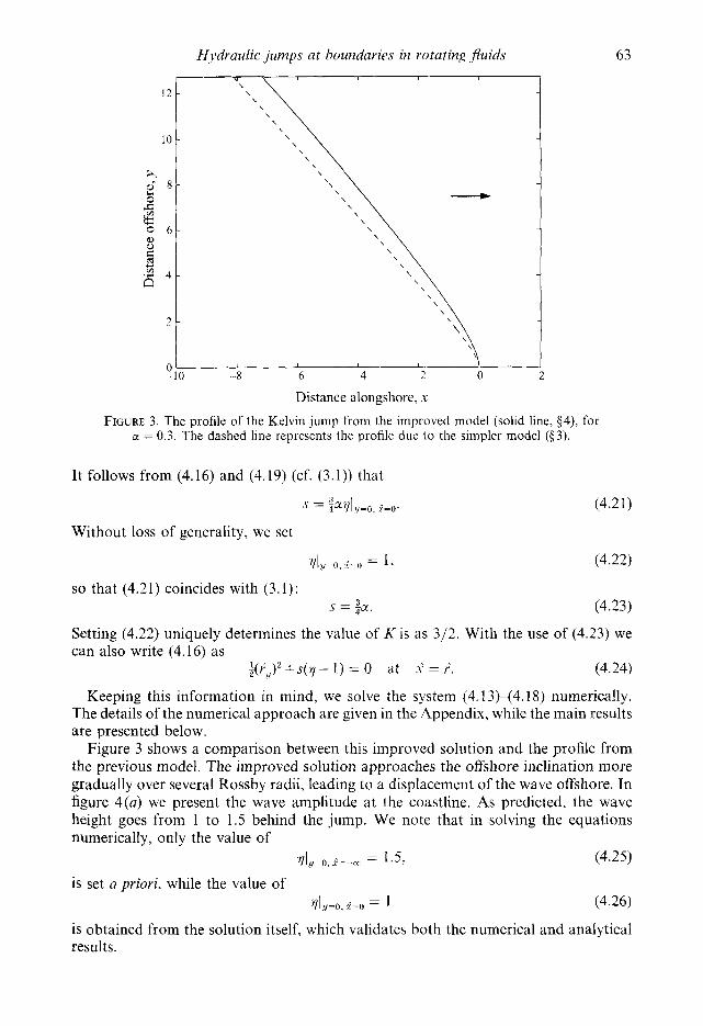
Distance alongshore, .x FIGURE 3. The profile of the Kelvin jump from the improved model (solid line, $4), for

a: = 0.3. The dashed line represents the profile due to the simpler model ($3).

It follows from (4.16) and (4.19) (cf. (3.1)) that

Without loss of generality, we set

&", j=" = 1.

so that (4.21) coincides with (3.1): s = 3a

4 -

(4.22)

(4.23)

Setting (4.22) uniquely determines the value of K is as 3/2. With the use of (4.23) we can also write (4.16) as

(4.24)

Keeping this information in mind, we solve the system (4.13)-(4.18) numerically. The details of the numerical approach are given in the Appendix, while the main results are presented below.

Figure 3 shows a comparison between this improved solution and the profile from the previous model. The improved solution approaches the offshore inclination more gradually over several Rossby radii, leading to a displacement of the wave offshore. In figure 4(a) we present the wave amplitude at the coastline. As predicted, the wave height goes from 1 to 1.5 behind the jump. We note that in solving the equations numerically, only the value of

?Ily=",+lr = 1.5, (4.25)

1 > f ( ? J + s(7 - 1) = 0 at s = t'.

is set a priori, while the value of YI?J=O,&lJ = 1 (4.26)

is obtained from the solution itself, which validates both the numerical and analytical results.

64

1.6

A . V. Fedorov and W. K. Melville

(a> 1.6 J

, + - (b) y = o

‘I ;A ,.Y=~.O ,’ I _ _ _ --. . , .._- I)------

y = 1.2 - - - - - - - - -

Figure 4(b) shows the wave height as a function of x at different distances offshore. One can see a striking difference compared with two-dimensional jumps, especially at distances of more than a Rossby radius offshore. At distances larger than the Rossby radius the wave profiles are similar to those for the linear Rossby adjustment problem (Gill 1982, p. 200).

Figure 5 displays the hydraulic jump and the wave field behind it. The pattern is similar to a numerical solution by Hermann et at. (1990), who considered the evolution of an initial disturbance described by shallow-water equations, including the effects of rotation and friction. In their solution the balance of friction and nonlinearity led to a steep front, propagating along the coast. Finally, in figure 6 we present the contour maps for the transverse velocity field. Note the concentration of the isolines behind the jump before the transverse velocity vanishes.

The last question we would like to consider is why the simplified model and our

Hj9druulic jumps at boundaries in rotating Puids 65

FIGURE 5. A Kelvin jump propagating along the coast (as viewed from the ocean). The graph displays the elevation of the free surface 7. The direction of propagation is shown by the arrow.


FIGURE 6. The contour map of the transverse velocity field behind the Kelvin jump for CL = 0.3. Positive values correspond to offshore flow.

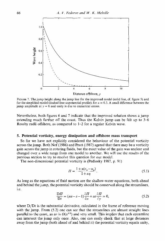
improved model give qualitatively similar results in describing the evolution of the wave front in space. Figure 7 shows the wave amplitude along the jump for the improved model and the simplified model (dashed line - exponential profile). While both decay for large y , a considerable difference is developed after 1-2 Rossby radii. We conclude that the rate of decay is not so important in describing the front evolution. The determining factor for the shape of the front is the jump amplitude at the coastline.

66 A. V. Fedorov and W. K . Melville

Distance offshore, y

FIGURE 7. The jump height along the jump line for the improved model (solid line, cf. figure 5) and for the simplified model (dashed lineeexponential profile), for a = 0.3. A small difference between the jump amplitude at y = 0 and unity is due to numerical errors.

Nevertheless, both figures 6 and 7 indicate that the improved solution shows a jump extending much further off the coast. Thus the Kelvin jump can be felt up to 3-6 Rossby radii offshore, as compared to 1-2 for a regular Kelvin wave.

5. Potential vorticity, energy dissipation and offshore mass transport So far we have not explicitly considered the behaviour of the potential vorticity

across the jump. Both Nof (1986) and Pratt (1987) agreed that there may be a vorticity gain across the jump in rotating fluids, but the exact value of the gain was unclear and changed over a wide range from one model to another. We will use the results of the previous section to try to resolve this question for our model.

The non-dimensional potential vorticity is (Pedlosky 1987, p. 91)

As long as the equations of fluid motion are the shallow-water equations, both ahead and behind the jump, the potential vorticity should be conserved along the streamlines, i.e.

an an - = (au-s- 1)-+av- = 0, Dt ax ay D n

where D/Dt is the substantial derivative, calculated in the frame of reference moving with the jump. From (5.2) one can see that the streamlines are almost straight lines parallel to the coast, as au is 0(01~'~) and very small. This implies that each streamline can intersect the jump only once. Also, one can easily check that at large distances away from the jump (both ahead of and behind it) the potential vorticity equals unity,


implying that the potential vorticity must remain uniform over the entire area. Thus there is no change in potential vorticity across the jump at all, although calculation of potential vorticity directly from the results of $4 will lead to some small non-zero value for the change owing to the neglect of higher-order terms in our solution. Also, this does not preclude the possibility of non-zero changes of potential vorticity for unsteady jumps.

Note that Pratt (1983) showed that the potential vorticity change across the jump is proportional to the tangential derivative of the third power of the local jump amplitude. However, in the context of our weakly nonlinear theory this change is negligible and cannot be detected.

Unlike the potential vorticity, energy should be lost in the jump. The value of the energy loss can be obtained from the two-dimensional theory. For example, the expression from Lighthill (1978, p. 179) in non-dimensional form gives the rate of energy loss per unit length and unit time as

= :a3[1113 + 0 ( ~ 4 ) . (5.3) Substituting 7 from the numerical solution for the improved model yields the rate of energy loss per unit time as

The dissipation is proportional to the third power of the jump amplitude, and for weak jumps is negligible.

Finally, we can calculate net mass transport offshore. Introducing the volume transport T, where

(5.5)

we can integrate (4.14) to obtain

Further, using the boundary conditions (4.17) and (4.18) gives

Now integrating (5.7) yields

T = sKe-y-$xK2ee2Y+Ceu,

where C is an arbitrary constant. Obviously,

TI,=, = 0,

and the transport should be finite for large y , which requires that

2s 3 a 2

K = - = -

(5.9)

(5.10)

and so that

(5.11) (5.12)


0.08

0.06

T(Y)

0.04

0.02

0

. -

1 2 3 4 5 6 I

Distance offshore, y FIGURE 8. The net flow offshore T(y) for a = 0.3. Analytical result - solid line, numerical

calculations - dot-dashed line.

That is, the net offshore flow is non-zero and is proportional to the jump strength. The plot of T ( y ) in figure 8 shows a maximum of the net offshore flow at a distance approximately equal to the Rossby radius.

6. The initial value problem: evolution of the Kelvin jump in space and time

We now proceed to consider the initial value problem for the jump evolution within the framework of the simplified model

6.1. The initial value problem : simplified model

pt+ppy = e-”, (6.1) with the boundary and initial conditions

where p = -ry. (6.4) Although these equations are derived under the assumption of small a, for simplicity we set a = 4/3, or alternatively we could transform (2.31) to (6.1) with a change of variables. The final results for a = 0.3 will be presented in the 56.2, figure 12.

Equation (6.1) is hyperbolic, and in general the initial-boundary value problem would have entirely continuous solutions only for some special initial conditions. We shall use the method of characteristics to solve the problem and rewrite (6.1) as

(ip2+e-Y)t+p(ip2+e-Y)y = 0. From (6.5) we see that

I 1 2+e-Y ZP


is conserved along the trajectory dY - _ dt -"

where Y = Yo. t o )

Y(t,i Yo, t o ) = Yo.

P = P ( t ; Yo, to).

P O = d t o ; Yw t o ) .

and y, is the position of the trajectory at a reference time to, i.e. It follows that along this trajectory

I = I -1 2 Now , - 2po+e-VoI where Using (6.6) and (6.1 I), we transform (6.7) to

which may be integrated to give

where

I eY/2 = - cosh ( t - to) + acosh eyoi2)}, p

acosh ( z ) = log (z + (2 - 1)'I2).

(6.10) (6.11) (6.12)

(6.13)

(6.14)

(6.15) Equation (6.14), together with (6.6) and (6.1 l), gives the general solution of the problem in parametric form.

Now we consider the case when the jump is initially a straight line normal to the coast, that is

pI+o = 0. (6.16) One can see that there will be two families of characteristics. The first is determined by the initial condition, and (6.14) reduces to

y = y,,+logcosh{te-'J2/x 2). (6.17) On characteristics of this type

p = [2(e-y0 - e-V)I1/2, (6.18) The second family is determined by the boundary condition, and (6.14) becomes

with y = 2logcosh{(t-to)/\ 2)

p = [2( 1 - e-y)]'i2.

(6.19)

(6.20) All characteristics are displayed in figure 9, which shows three different regions. The solution in region (I) is only influenced by the boundary condition; in region (11) only by the initial condition, and in region I11 by both. This implies that in this middle region we have multi-valued solutions. To avoid this we must introduce a break in the solution, so that p experiences a jump. This is analogous to the appearance of shock-shocks in gas dynamics (Whitham 1974, p. 289).

To find the location of the break, say Y = Y(t), we integrate (6.1) across this jump as was done in the previous section. The procedure gives

(6.21)

where [PI =PI y=Y+O y=Y-O' (6.22)


4 2 0

Y FIGURE 9. Two families of characteristics. The overlap in area (111) may result

in multi-valued solutions.

6 4 2 0

Y FIGURE 10. The final characteristic pattern with the boundary separating

the two families of characteristics.

Hydraulic jumps at boundaries in rotating ju ids 71

1.6

1.2

0.8

0.4

6 4 2 0

t - 6.0 I-I 3 2 1 0

Distance offshore, y FIGURE 1 1. (a) The solution of the initial value problem showing the shape of the jump at different times for the simplified model ( r = r ( y , t ) ) . Initially the jump is a straight line normal to the coast. a = 4/3 is taken for simplicity of the analytical formulae. Similar results for a = 0.3 are presented in figure 12. (b) The absolute value of the derivative &/?y at different times for a = 4/3.

It follows from (6.21) that - - 1 dY dt - 'I(PIy=y-o +Plu=Y+o). (6.23)

Using (6.18) and (6.20) we can rewrite this as

- ;([2(1 -e-')]l/'+ [2(e-yo-e-Y)]1/2), (6.24)

where Y = Y,+Iogcosh(te-'u''/~~2}. (6.25) Solving (6.24)-(6.25) numerically with respect to Y, we find the location of the boundary, which separates the two families of characteristics. The characteristic pattern with the boundary is displayed in figure 10. The characteristics give the entire solution of the problem in parametric form, shown in figure l l ( u , b) at different times, in terms of both p and r .

dY - _ dt

72 A. V . Fedorov and W. K. Melville

One can see how an initially straight line gradually bends. With time it develops a kink: a break in the derivative which corresponds to the boundary between the characteristic families (or the shock-shock). From (6.20) (compare with (3.2)) it is clear that from the coastline to the kink our solution is simply the steady translating shock described in the previous section. With time the kink propagates offshore. This means that after some adjustment time the Kelvin shock acquires a permanent form over any finite distance from the shore. We can state the more fundamental result for (6.1)-(6.3) that, regardless of its initial profile in space, a Kelvin shock evolves into a steady shock, determined by expressions (3.3 j(3.5), with its permanent form depending only on the shock amplitude.

To show this result let us consider the characteristics determined by an arbitrary initial condition (i.e. setting to = 0 in (6.14))

(+Z)l/’ t + acosh (I:” eYoI2))

We assume that initially the offshore scale of the jump is bounded, i.e.

as is the derivative drldy, with Yo d Po

Po bw

(6.26)

(6.27)

(6.28)

where 9, and bo are given. Then for sufficiently large times (6.26) reduces to

y z t(2Z0)1’2. (6.29)

This implies that the region where

y d t(21min)?

with Zmin = min(Zo) > 0,

(6.30)

(6.31)

will not be covered by the characteristics of this type (region I in figure 10). Thus the width of the coastal region, unaffected by the initial condition, grows at least linearly with time. The solution there must be determined by the boundary condition, and it is the steady wave solution described earlier. Finally, note that the constraints (6.27) and (6.28) are not really restrictive, as 3, and 6, can be arbitrarily large.

with

and

6.2. The initial value problem : the improved model As we have already seen, the simplified model does not describe adequately the wave field behind the jump. Following the procedure of $4, we can derive a full system of evolution equations describing the jump and the wave field behind. Using conventional methods of perturbation theory and assuming that the time dependence is slow gives

(6.32) vt = V,--Ty-?l, (6.33)

(6.34)

v=O at y=O,oo, (6.35)

= sy, - 2s77, + ;(v - Oy),

; t - L ” - 2(ry)2 + 4% - 11,

v = - y ^ y ~ at 2 = ?, V - K ~ - ~ as 2+-m,

(6.36) (6.37)

T o = 7 l M . (6.38)

Hydraulic jumps at boundaries in rotating fluids

3

t

73

Distance offshore, y FIGURE 12. The numerical solution of the initial value problem showing the shape of the jump at different times (improved model, cf. 94). Initially the jump is a straight line normal to the coast. Dashed lines show the jump locations obtained from the simplified model (cf. 93) , for cr. = 0.3.

The absolute position of the jump is given by (cf. (4.2))

R = t+r(y , t ) = t+~ t+v^ (y , t). (6.39)

Only (6.32) and (6.33) are new. For the derivation of similar equations see Tomasson (1991) and Fedorov & Melville (1995). In the stationary limit (6.32)-(6.33) become (4.13)-(4.14). Equation (6.34) corresponds to one of the boundary conditions of the steady problem (cf. (4.24)) and, in fact, is one of the jump conditions (cf. (2.23)). All the remaining boundary conditions are in place. The motion of the jump is determined by (6.34), and is coupled with (6.32) and (6.33) through the wave amplitude yo(y) along the jump. As the initial condition we choose

y = Ke-”, (6.40)

which is different from the simplified model by a factor of K (see 94). Nevertheless, in figure 12 one can see that there are no qualitative differences between the evolution of the fronts described by the two models. This is due to the fact that after a very short time that part of jump near the coast turns into a steadily translating jump, as it does in the simplified model. The dynamics of the jump in the simplified and the improved models turn out to be almost the same and may be described through the method of characteristics. The comparison in figure 12 shows qualitative agreement. Also note that the solid and dashed lines in figure 12 become parallel at longer times at larger distances offshore (cf. figure 3).

7. Strongly nonlinear case: simplified model When the jump is strong, and the nonlinearity is not weak, we cannot complete the

perturbation analysis of 932 and 4. Nevertheless, as long as the offshore velocity remains relatively small, a similar approach may work even for strong nonlinearity. To


construct such a theory we use the full shallow-water equations, again for a single-layer fluid :

U , + MU, + vu, +gh, - fv = 0, V , + MU, + V V , + gh, +fu = 0,

h, + (uh), + (vh), = 0.

(7.1) (7.2) (7.3)

The notation is conventional (Pedlosky 1987, p. 61), with h(x ,y , t ) denoting the entire local height of the layer. In conservation form the equations become (Pratt 1983, for example)

(uh), + ( U 2 h + gihZ), + (uvh), -fvh = 0, (vh), + (uvh), + (v2h +gih2), +fuh = 0,

h, + (uh), + (vh), = 0.

(7.4) (7.5) (7.6)

Assuming that the jump is moving into still water of constant depth d, we integrate the equations across the jump located at x = R ( y , t) , and obtain

where

R,u,-u~-agH+R,u,v, = 0, R,v,-u,v,+R,v2,+RyagH = 0,

Rta-u,+R,v, = 0,

H = ;(ha + d),

(7.7) (7.8) (7.9)

(7.10)

a = @,-4/h, , (7.11)

and h, is the height of the wave field behind the jump, i.e.

ha = hlx=E-O. (7.12)

Both a and H, together with other parameters behind the jump, are functions of y .

(R, - U, + R, v,) (v, + R, u,) = 0.

Now we multiply (7.7) by R, and add (7.8) to give

(7.13)

Taking (7.9) into account, (7.13) implies that

v,+Ryu, = 0, (7.14)

which simply means that the velocity component tangential to the jump does not experience any break. This equation is equivalent to (2.20) of the weakly nonlinear theory.

Using (7.14) in (7.7) and (7.8) yields

R, u, - agH = ui( 1 + Ri), (7.15)

and R, a = u,( 1 + Ri). (7.16)

It follows that agH u, = (1 -a) R, ’

Substituting (7.17) into (7.16) gives an equation for R:

(7.17)

(7.18)

(7.19) For steady wave solutions

R, = U,



FIGURE 13. The jump profiles for different amplitudes: A = 0.3, 1, 3, 5.

0.2

0.6

- I'

0.4

0.2

0

. A = 0.3

Distance offshore, y 5

FIGURE 14. The non-dimensional transverse velocity i; = U,/C as a function of y in the area of the jump for different jump amplitudes: A = 0.3, 1, 3, 5.

76 A . V. Fedoovov and W. K. Melville

agH (1 -a) U ’

u, =

and (1 -a) U 2 g H

R; = - 1,

where from the no-flow boundary condition

(7.20)

(7.21)

(7.22)

We assume that the transverse momentum balance behind the jump is geostrophic:

gh,+fu = 0. (7.23)

Although this may not be true immediately behind the jump, by analogy with the weakly nonlinear case we still expect the profile of the jump to be described relatively well, provided the transverse velocity is small.

To satisfy (7.23) we use the expression for u from (7.20) and the assumption that u depends only on y behind the jump to give

(7.24)

Finally, we define the non-dimensional height, 5, of the fluid layer, where

5 = hold, (7.25)

and rewrite (7.21) and (7.24), making use of (7.22) and (7.25), to give

(7.26)

with Q = 51y=o’ (7.27)

and -+-($- d5 f 1) = 0. dy 2U

(7.28)

We introduce a Rossby radius of deformation

Ro = U / f , (7.29)

based on the nonlinear speed of the jump, and solve (7.28) to obtain

(7.30)

with C0 = 1 + A , (7.31)

where A is a non-dimensional amplitude. In the weakly nonlinear case A z a, and the elevation of the free surface is exponentially decaying offshore in the manner of a Kelvin wave.


The connection between the jump amplitude and jump velocity is now

U 2 = gd(1 + A ) ( 1 +;A), (7.32)

which is similar to the regular two-dimensional hydraulic jump (see Lighthill 1978, p. 177). From (7.26) and (7.30) we obtain the value of Ri as y - t CD :

R; = $(A + 3) A .

4 = atan [;(A + 3) All''.

A = ;(-3+2/'17) z 0.56

(7.33)

(7.34)

Thus the angle between the jump and the normal to the coast is

When the amplitude A is small and A z a, formula (7.34) reduces to (3.5) of the weakly nonlinear model. When

(7.35)

the angle of inclination becomes 45". Figure 13 displays the shape of the shocks for different values of A (cf. figures 2 and 3 for weak nonlinearity). Clearly, y5 increases as the amplitude and the jump speed increase. The lateral extent of the region in which the jump is almost normal to the coast gradually decreases.

Returning to (7.2) and (7.8), and checking our assumptions of applicability of the geostrophic approximation, we introduce u" as

(7.36) d = C(y) = v,/c,

with c = (gho)l'2, (7.37)

which is the phase speed of long gravity waves in the absence of rotation. The parameter 6 is a non-dimensional transverse velocity in the neighbourhood of the jump, and acts as a local Rossby number with respect to the y-momentum equation. Therefore, we expect that the smallness of 6 (smallness of the transverse velocity) may still guarantee the validity of the solution. From figure 14 it can be seen that 6 remains relatively small for amplitudes A smaller than unity. Note, that 6 does not depend upon d or g, but only upon A .

8. Examples : simplified model, strong nonlinearity First, we consider a moderately nonlinear jump for physically reasonable ocean

parameters, say A = 0.2, d = 100 m and g = 0.01 m s - ~ (effective gravity for internal waves), corresponding to Ro z 10 km. Figure 15(a) gives the values of u,,, 0,

and c as functions of y and the jump speed U for this case. Clearly, the jump is accompanied by a relatively strong alongshore current. The speed of the jump remains slightly higher than the speed of long gravity waves in the absence of rotation. The Kelvin jump is accompanied by a moderate transverse flow offshore, which remains weaker than the alongshore current. We can estimate the extent of the region with non- zero transverse velocity behind the jump as Ro All2 , which is almost half of the Rossby radius for this particular case.

The second example is a much stronger jump with the relative amplitude A = 3.0 (figure 15h). One can see that we have now very strong alongshore and offshore flows, and the jump moves at about twice the speed of long gravity waves. Although this case is unlikely to occur in nature, it clearly shows the tendencies associated with the growth of the jump amplitude. Another reason for considering this case is to demonstrate how the alongshore current becomes supercritical at the coast.


. . . . . . . . . . . . . , . . . . . . . . . . . . . . . . . . . . . . . . . . . . . . . . . . . . . . . . . . . . . . . . . . . . . . . . . . . . . . . . . .. . . . . . . . . . . . . . . . . . . 1.2

0 10 20 30

Distance offshore (km) FIGURE 15. The values of the characteristic velocities behind the jump u, (-), u0(---) and c (-.-.-), as functions of y , and the jump speed U (......) for (a) A = 0.2, (b) A = 3 .

9. Summary and conclusions We have shown that, with relatively weak assumptions, a class of Kelvin shocks

exists in a rotating semi-infinite ocean. Regardless of its initial profile, the shape of the jump tends to that of a steadily translating jump followed by a stationary wave field. The Kelvin shocks have the following properties.

(i) In the lee of the jump, the wave field decays exponentially offshore in a manner similar to that of a Kelvin wave.

(ii) The jump travels with a constant speed and maintains a permanent shape, which depends only on the jump strength.

(iii) The jump curves back from the normal to the coast to a straight oblique line offshore. The angle included between the normal and the jump offshore is a simple function of the amplitude at the coast.

(iv) The effect of the Kelvin jump can be felt up to 3-6 Rossby radii offshore, compared to 1-2 for a regular Kelvin wave.

Hjdraulic ,jumps at boundaries in rotating fluids 79

(v) Potential vorticity does not change across the jump. This follows from the properties of the solution, and is not assumed (1 priori.

(vi) The Kelvin jump gives rise to a moderate offshore flow. The flow is local in the sense that it arises only in the rear of the jump and then vanishes at a distance proportional to the square root of the jump amplitude. The net offshore flow is non- zero. This feature is different from that of regular Kelvin waves (cf. Fedorov & Melville 1995), which have zero net transverse flow.

(vii) The Kelvin jump represents a discontinuous solution of the full shallow-water equations in a semi-infinite rotating ocean with the discontinuity obeying mass and momen tum conservation.

As we have seen, the Kelvin-type hydraulic jump studied here precedes an alongshore flow, which to leading order is in geostrophic balance. The jump leads the current. Another possibility would be a jump separating two regions of geostrophic current. It may be plausible that such a jump can remain stationary relative to the coast, provided the flow is to the right as observed from the coast. There may be differences in the equations arising from the nonlinear character of the problem. Nevertheless, the main flow. at least for weak nonlinearity, is described by linear geostrophic equations. To such a current we can always add another geostrophic current flowing in the opposite direction at a uniform speed, corresponding to a constant slope of the isopycnals. We could choose this extra current so that the hydraulic jump will not move with respect to the coast.

The shape of the Kelvin jump solutions, especially for larger amplitudes, has a strong resemblance to the satellite imagery of some atmospheric disturbances propagating to the north along the western coast of North America (Mass & Albright 1987). These disturbances are revealed by overcast areas of the marine atmospheric layer bounded inland by coastal mountain ranges. The shape of the northern front of the overcast is usually similar to the Kelvin jump.

This work was supported by a grant from the Office of Naval Research, Coastal Sciences. We are grateful to Larry Pratt and anonymous referees for many helpful comments on the first version of the paper.

Appendix. Numerical scheme

instead o f ? we introduce a new independent variable: When solving the system (4.13)-(4.18) or its time-dependent equivalent (6.32)-(6.37),

5 = .i? - i, (A 1)

and use

and

This allows us to write the boundary conditions at fixed boundaries. Thus the set of unsteady equations (6.32)-(6.37), for example, can be rewritten as

80

Further, we introduce an artificial friction with the coefficients v and p:

A . V. Fedorov and W. K. Melville

a9t - 49,, + ryJ = (3 + cr̂ tt> 96 - 2S99[ + fiy vg + fCV - uy),

but - v(v,, + uy,> = ug + tv 9s - 9 y - 9,

(A 7)

(A 8)

cr̂ , = ;(?J +$(TO - 1). (A 9)

Equations (A 7)-(A 9) are solved on a non-uniform grid (xn, y,) with local resolution (Axn, Ay,). Usually, we put more grid points near the coast and the jump. We use a scheme similar to MacCormac’s scheme (explicit scheme of the predictor-corrector type, see Fletcher 1988). The difference is that the nonlinear convective term in (A 7) is given by centred finite differences. The scheme has second-order accuracy in both space and time.

The viscous coefficients in (A 7)-(A 9) are

and

Such friction adds extra terms to the equations, comparable to numerical errors due to finite differencing. It decreases at higher resolutions of the grid. Non-zero friction also serves the purposes of eliminating free waves, which may reflect from the boundaries of the ocean basin. Numerical tests demonstrated that the results presented here are insensitive to the details of the friction terms.

We have also introduced parameters a, b and c in (A 7)-(A 9). These parameters are equal to unity for the initial value problem in 96.2. To obtain steady solutions we let a, b and c be functions of position, which speeds up convergence.

The boundary conditions are defined as

where ymas and t,,, determine the numerical boundaries of the ocean basin. We usually set them in the range 1&15.

The scheme is found to be stable for time steps smaller than

with

At d q min (Axn, Ay,)

q - 0.3-0.6.

To obtain the stationary solution we run the program long enough for the solution to converge to a steady solution. The calculations are stopped as soon as the terms proportional to temporal derivatives in (A 7)-(A 9) become much smaller than numerical errors due to finite differencing.

Finally, to check the validity of the numerical approach we take advantage of two integrals for the problem. The first is the net offshore flow, for which we have an explicit analytical expression. Its comparison with the numerical result is given in 95. Another integral constraint can be obtained by integrating (4.13) with the boundary conditions to give

t = @, (1 - 9 ) d t f c o n s t .

Hvdraulic jumps at boundaries in rotating JEuids 81

-3 -2 -1


FIGURE 16. A comparison between F obtained by direct numerical calculations (solid line), and r^ obtained from (A 17) (dot-dashed line).

Figure 16 shows a good match between r^ calculated directly, and r^ obtain from (A 17). Some error is due to the finite resolution of the scheme and the finite size of the ocean basin we use.

R E F E R E N C E S

ARMI, L. 1986 The hydraulics of two flowing layers with different densities. J . Fluid Mech. 163,

ARMI, L. & FARMER, D. M. 1985 The internal hydraulics of the Strait of Gibraltar and associated

BAINES, P. G. 1980 The dynamics of the southerly buster. Austral. Met. Mug. 28, 175-200. BANNON, P. R. 1981 Synoptic scale forcing of coastal flows: forced double Kelvin waves in the

atmosphere. Q. J. R. Met. Soc. 107, 313-327. BEARDSLEY, R. C., DORMAN, C. E., FRIEHE, C. A., ROSENFELD, L. K. & WINANT, C. D. 1987 Local

atmospheric forcing during the CODE, 1 , A description of the marine boundary layer and atmospheric conditions over a northern California upwelling region. J . Geophys. Res. 92,

27-58.

sills and narrows. Oceanologica Acta 8, 3746.

1467-1488. BENNET, J. R. 1973 A theory of large-amplitude Kelvin waves. J . Phys. Oceanogr. 3, 57-60. BENNETT, A. F. & CUMMINS, P. F. 1988 Tracking fronts in solutions to the shallow water equations.

J . Ceophys. Res. 93, 1293-1301. CHOW, V.-T. 1959 Open-Channel Hydraulics. McGraw-Hill. DORMAN, C. E. 1987 Possible role of gravity currents in northern California’s summer wind

FEDOROV, A. V. & MELVILLE, W. K. 1995 On the propagation and breaking of nonlinear Kelvin

FLETCHER, C. A. J. 1988 Computational Techniques for Fluid Dynamics. Springer. GARVINE, R. W. 1987 Estuary plumes and fronts in shelf waters: A layer model. J . Phys. Oceunogr.

17, 1877-1896. GILL, A. E. 1977 Coastally trapped waves in the atmosphere. Q. J . R . Met. SOL. 103, 431440. GILL, A. E. 1982 Atmosphere-Ocean Dynamics. Academic.

reversals. J. Ceophys., Res. 92, 1497-1505.

waves. J . Phys. Oceanogr. 25, 2518-2531.


HERMANN, A. J., HICKEY, B. M., MASS, C. F. & ALBRIGHT, M. D. 1990 Orographically trapped coastal wind events in the Pacific Northwest and their oceanic response. J. Geophys. Res. 95,

HOUGHTON, D. D. 1969 Effect of rotation on the formation of hydraulic jumps. J . Geophys. Res. 74,

LIGHTHILL, M. J. 1978 Waves in Fluids. Cambridge University Press. MASS, C. F. & ALBRIGHT, M. D. 1987 Coastal southerlies and alongshore surges of the west coast

NOF, D. 1984 Shock waves in currents and outflows. J . Phys. Oceanogr. 14, 1683-1702. NOF, D. 1986 Geostrophic shock waves. J. Phys. Oceanogr. 16, 886901. O’DONNELL, J. 1989 Transients in the nonlinear adjustment to geostrophy. In The Physical

PARRET, C. A. & CULLEN, M. J. P. 1984 Simulation of hydraulic jumps in the presence of rotation

PEDLOSKY, J. 1987 Geophysical Fluid Dynamics. Springer. PRATT, L. J. 1983 On inertial flow over topography. Part 1. J . Fluid Mech. 131, 195-218. PRATT, L. J . 1987 Rotating shocks in a separated laboratory channel flow. J. Phys. Oceanogr. 17,

RENOUARD, D. P., TOMASSON, G. G. & MELVILLE, W. K. 1992 An experimental and numerical study

13 169-13 193.

135 1-1 360.

of North America. Mon. Weath. Rev. 115, 1707-1738.

Oceanography of the Sea Straits (ed. L. J. Pratt), pp. 509-516. Kluwer.

andmountains. Q. J . R. Met. SOC. 110, 147-165.

483-491.

of nonlinear internal waves. Phys. Fluids A 5 , 1401-1411. STERN, M. E. 1980 Geostrophic fronts, bores, breaking and blocking waves. J. Fluid Mech. 99,

687-703. STOKER, 3. J. 1957 Water Waves. Interscience. TOMASSON, G. G. 1991 Nonlinear waves in a channel: three-dimensional and rotational effects. Ph.D

thesis, Dept of Civil Engineering, MIT. TOMASSON, G. G. & MELVILLE, W. K. 1992 Geostrophic adjustment in a channel: Nonlinear and

dispersive effects. J. Fluid Mech. 241, 23-57. WELANDER, P. 1961 Numerical prediction of storm surges. Adv. Geophys. 8, 316-379. WHITHAM, G. B. 1974 Linear and Nonlinear Waves. Wiley.

Documents

Hydraulic jumps at boundaries in rotating fluids · with the jump amplitude as the small parameter, applied both to the wave field behind the jump and to the matching conditions