University of South FloridaScholar Commons

Graduate Theses and Dissertations Graduate School

June 2018

Hydraulic Performance and Vulnerability onSanitary Sewer Overflow in Southern PinellasCounty, FLUchechi O. AkaboguUniversity of South Florida, uakabogu@mail.usf.edu

Follow this and additional works at: https://scholarcommons.usf.edu/etd

Part of the Civil Engineering Commons

This Thesis is brought to you for free and open access by the Graduate School at Scholar Commons. It has been accepted for inclusion in GraduateTheses and Dissertations by an authorized administrator of Scholar Commons. For more information, please contact scholarcommons@usf.edu.

Scholar Commons CitationAkabogu, Uchechi O., "Hydraulic Performance and Vulnerability on Sanitary Sewer Overflow in Southern Pinellas County, FL"(2018). Graduate Theses and Dissertations.https://scholarcommons.usf.edu/etd/7256

Hydraulic Performance and Vulnerability on Sanitary Sewer Overflow

in Southern Pinellas County, FL

by

Uchechi O. Akabogu

A thesis submitted in partial fulfillment

of the requirements for the degree of

Master of Science in Civil Engineering

Department of Civil and Environmental Engineering

College of Engineering

University of South Florida

Major Professor: Mahmood H. Nachabe, Ph.D.

Mauricio Arias, Ph.D.

Kenneth Trout, Ph.D.

Date of Approval:

June 8, 2018

Keywords: Base Infiltration, Dry Weather Flow, Reliability

Copyright © 2018, Uchechi O. Akabogu

DEDICATION

I will like to dedicate this work to myself, proving that I can accomplish anything if I

believe and work hard on it. I will also like to dedicate this work to my family for their patience,

encouragement, and support.

ACKNOWLEDGMENTS

I will like to thank Dr. Mahmood Nachabe for his encouragement, support, and valuable

guidance throughout the entirety of the study. I will also like to thank the members of my

committee, Dr. Mahmood Nachabe, Dr. Mauricio Arias and Dr. Kenneth Trout for their time,

support and effort. I believe that I learned a lot from working on this project, and will never

forget the experience, struggles, and accomplishments. More so, will like to thank the CHI

network for giving me a university grant to explore and use PC SWMM software for my study. It

was an excellent exposure to hydraulic modeling, and I liked and enjoyed using the program.

i

TABLE OF CONTENTS

LIST OF TABLES .......................................................................................................................... ii

LIST OF FIGURES ....................................................................................................................... iii

ABSTRACT .....................................................................................................................................v

CHAPTER 1: INTRODUCTION ....................................................................................................1

1.1 Scale of Sanitary Sewer Overflow .................................................................................2

1.2 Cause of Sanitary Sewer Overflow ................................................................................2

1.3 Reduction of Sanitary Sewer Overflow .........................................................................3

1.4 Objective of the Study ...................................................................................................4

1.5 Literature Review...........................................................................................................4

1.5.1 Modeling Method............................................................................................4

CHAPTER 2: MATERIALS AND METHODS .............................................................................7

2.1 Case Study Area and Infrastructure ...............................................................................7

2.2 Instrumentation ..............................................................................................................7

2.2.1 Flow Meters ....................................................................................................7

2.2.2 Rain Gages ......................................................................................................8

2.2.3 Groundwater Monitoring Wells ......................................................................8

2.3 Methods ......................................................................................................................9

2.3.1 Time Series Analysis ......................................................................................9

2.3.2 Cross-Correlation and Regression Analysis .................................................11

2.3.3 PC SWMM Model Analysis .........................................................................12

2.3.3.1 Flow Routing Methods ..................................................................12

2.3.3.2 Flow Inputs ....................................................................................14

2.3.3.3 Geometric Parameters ....................................................................16

CHAPTER 3: ANALYSIS RESULTS ..........................................................................................17

3.1 Cross-Correlation and Regression Analysis ................................................................17

3.2 PC SWMM Model Analysis ........................................................................................20

CHAPTER 4: CONCLUSION ......................................................................................................26

LIST OF REFERENCES ...............................................................................................................28

APPENDIX A: SUPPLEMENTAL FIGURES .............................................................................30

ii

LIST OF TABLES

Table 1: Different rainfall depths for different hurricane events ...................................................19

Table 2: Sewer system hydraulic performance indicators for different rainfall depths .................23

iii

LIST OF FIGURES

Figure 1: PS-119 (the outfall) sanitary sewer layout .......................................................................9

Figure 2: Average residual flow for significant rainfall events .....................................................11

Figure 3: Diurnal pattern simulated using PC SWMM .................................................................14

Figure 4: PS-119 simulated average DWF from June 1st-September 30th ....................................15

Figure 5: Cross-correlation between BI and rain during wet weather periods ..............................17

Figure 6: Regression model to predict BI at PS-119 .....................................................................18

Figure 7: BI distribution for different rainfall depths ....................................................................20

Figure 8: PS-119 simulated time series graph, DWF+BI from June–September 2016 .................21

Figure 9a: Hydraulic profile of flow surcharge downstream on June 10th ....................................21

Figure 9b: Hydraulic profile of flow surcharge downstream on September 1st .............................22

Figure 10a: Hurricane Harvey rainfall depth .................................................................................24

Figure 10b: 40-inches rainfall depth ..............................................................................................24

Figure 11: Flow hydrographs of the different rainfalls depths vs. PS-119 design capacity ..........25

Figure A1: Cross section of surcharged manhole ..........................................................................30

Figure A2: Cross section of ponded/overflowed manhole ............................................................30

Figure A3: Rainfall intensity from February-September 2016 ......................................................31

Figure A4: Total observed flow and BI for PS-119 .......................................................................31

Figure A5: Hurricane Matthew rainfall depth ...............................................................................32

Figure A6: Hurricane Matthew rainfall depth ...............................................................................32

iv

Figure A7: Hurricane Hermine rainfall depth ................................................................................33

Figure A8: Hurricane Hermine rainfall depth ................................................................................33

Figure A9: Hurricane Irma rainfall depth ......................................................................................34

Figure A10: Hurricane Irma rainfall depth ....................................................................................34

Figure A11: 25-inches rainfall depth .............................................................................................35

Figure A12: 25-inches rainfall depth .............................................................................................35

Figure A13: 30-inches rainfall depth .............................................................................................36

Figure A14: 30-inches rainfall depth .............................................................................................36

Figure A15: Hurricane Harvey rainfall depth ................................................................................37

Figure A16: 40-inches rainfall depth .............................................................................................38

v

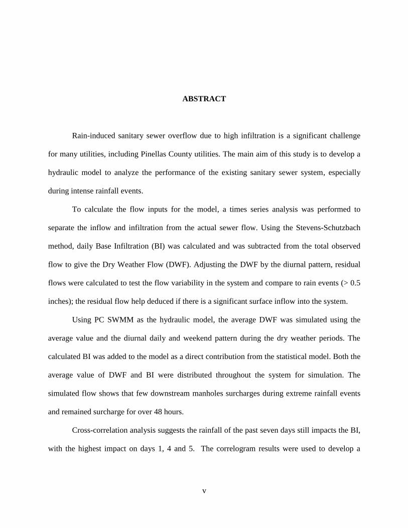
ABSTRACT

Rain-induced sanitary sewer overflow due to high infiltration is a significant challenge

for many utilities, including Pinellas County utilities. The main aim of this study is to develop a

hydraulic model to analyze the performance of the existing sanitary sewer system, especially

during intense rainfall events.

To calculate the flow inputs for the model, a times series analysis was performed to

separate the inflow and infiltration from the actual sewer flow. Using the Stevens-Schutzbach

method, daily Base Infiltration (BI) was calculated and was subtracted from the total observed

flow to give the Dry Weather Flow (DWF). Adjusting the DWF by the diurnal pattern, residual

flows were calculated to test the flow variability in the system and compare to rain events (> 0.5

inches); the residual flow help deduced if there is a significant surface inflow into the system.

Using PC SWMM as the hydraulic model, the average DWF was simulated using the

average value and the diurnal daily and weekend pattern during the dry weather periods. The

calculated BI was added to the model as a direct contribution from the statistical model. Both the

average value of DWF and BI were distributed throughout the system for simulation. The

simulated flow shows that few downstream manholes surcharges during extreme rainfall events

and remained surcharge for over 48 hours.

Cross-correlation analysis suggests the rainfall of the past seven days still impacts the BI,

with the highest impact on days 1, 4 and 5. The correlogram results were used to develop a

vi

regression model, to predict the BI for different rainfall depths, which in turn was used for

hydraulic performance analysis.

Increasing the rainfall depths and routing the flow using PC SWMM, showed that the

hydraulic grade line, number and hours of the surcharged manholes increases as total rainfall

depths increases, but no sanitary sewer overflow. Sanitary sewer overflow occurred at the lift

station with a design capacity of 200 GPM for all increased rainfall depths. Furthermore, the

analysis results can help locate areas where overflow is more likely to occur, and can also help

plan and implement a cost-effective rehabilitation program for the existing sewer network.

1

CHAPTER 1: INTRODUCTION

One of the challenges facing by municipalities across the United States is the issue of

Sanitary Sewer Overflow. Sanitary Sewer Overflow (SSO) is an unauthorized discharge of

untreated wastewater from a collection system or wastewater treatment facility, which poses

serious public health and environmental problems. According to Petrequin (2011), an estimate of

40,000 overflows occurs per year, and at least one-third of the nation’s wastewater treatment

municipalities faced fines or disciplinary measures for sewage violations. Due to the risk posed

to public health, SSO has been linked to roughly 8.6 million cases of waterborne illness per year

(Peterquin, 2011) diseases that range in severity from mild gastroenteritis to life-threatening

illness such as cholera, dysentery, infectious hepatitis, and severe gastroenteritis (EPA, 2004).

From a legal perspective, section 301 (a) of the Clean Water Act prohibits unpermitted

discharge of pollutants. Furthermore, The National Pollutant Discharge Elimination System

(NPDES) allows discharge under certain specific conditions which usually includes an effluent

limit, and requires all permittees to properly operate, adhere and maintain all facilities, impose

self-monitoring, and reporting requirements (EPA, 1995). SSO is as result of surcharge overflow

in the sanitary sewer conveyance system. Sanitary sewer collection and conveyance system

surcharges when the hydraulic grade line of the system rises to the ground surface level, because

the actual flow exceeds the design capacity of the system. The sewer surcharges can occur at

junctions such as manholes, pipe fittings, and outlets, collection wells and treatment facility.

2

1.1 Scale of Sanitary Sewer Overflow

Sanitary sewer surcharge at a junction such as; manhole, cleanout or pipe fitting, results

to SSO when the flow changes from free surface flow to pressurized flow. As the pressure

increases, the water level rises until it raises to the surface, diffusing the build-up pressure, thus,

SSO. Furthermore, sewer surcharge can occur at the collection wells and at the wastewater

treatment facility when the flow exceeds the pumping capacity and volume capacity of the

treatment facility respectively. In September 2017, Hurricane Harvey delivered 40-61inches of

rain across Texas, which led to approximately 150 million gallons of both SSO and industrial

discharge into the environment (TCEQ, 2017). In September 2016, an estimated combined

volume of 240 million gallons of partially or untreated sewage was dumped into the Tampa Bay

during Hurricane Hermine, which delivered up to 22 inches of rain in some parts of the Tampa

Bay area (Neuhaus, 2016).

1.2 Cause of Sanitary Sewer Overflow

As stated above, SSO results from surcharge when the hydraulic grade line rises to the

ground surface elevation. SSO occurs during the wet weather due to Rain Derived Inflow and

Infiltration (RDII), blockages, cracked pipes and manholes, structural, mechanical and electrical

failures and insufficient conveyance capacity. Reduction in pipe capacity caused by blockage

often exacerbate surcharging and backups by causing a build-up of debris such as wood logs,

plastic bags, household waste and solidified grease.

RDII is rain-induced inflow and infiltration entering the sewer system, usually during wet

weather events. Surface runoff (inflow) enters the sewer system via cleanouts, unsealed

manholes or illegal connections. Inflow into the system is evident in the flow hydrograph as a

fast increase or response in the flow rate during the duration of a rain event and quickly subsides

3

after the rain event. Infiltration is the inflow of groundwater into the sewer pipe and increases

with the water table elevation. Groundwater infiltration is associated with soil water or

groundwater that seeps into the sanitary sewer through cracks in the pipes, manholes, or wet

wells. When the pipe or well is submerged beneath the water table, it creates a positive pressure

higher than the atmospheric pressure, thus creating a pressure gradient. This pressure gradient

drives the groundwater through cracks and holes into the pipe, leading to infiltration in the sewer

pipes. Unlike surface inflow, infiltration in the system shows a slower but persistent response in

the flow hydrograph with a rain event.

1.3 Reduction of Sanitary Sewer Overflow

Many programs and designs have been introduced to reduce the SSO at different scales.

One of the methods is to maximize the capacity of flow. Maximizing the flow capacity can be

accomplished by two methods: utilizing storage facilities and increasing the flow carrying

capacity. Due to high volumes and variability caused by RDII, additional wastewater storage

facilities can be considered as a control for SSO. The additional storage facility is feasible

because it requires relativity low-cost construction and maintenance and can operate regardless

of the random high-intensity rain events. The only disadvantage is that the storage facilities are

relatively large and requires a large area of land. Increasing the flow carrying capacity includes

monthly/daily maintenance and cleaning out the clogged pipes, increasing the pumping capacity,

and replacing the existing pipes with high diameter pipes.

Another method for reducing SSO is rehabilitation strategy. Rehabilitation involves

lining pipes segments to reduce infiltration induced by an increase in water table via cracks in the

pipes, manholes and joint fitting. The advantage of rehabilitation is that it reduces the infiltration

rate in the pipes thus reducing the volume of the sewer flow, increasing the efficiency of the

4

treatment facility; hence reduce SSO during extreme events. The disadvantage of rehabilitation

is cost. Because of limited resources, one of the challenges of rehabilitation is prioritizing which

pipe segment to rehabilitate first to maximize the reduction of SSO.

1.4 Objective of the Study

The objective of the study is to perform system failure analysis on one of the sewershed

located in South Pinellas County by developing a hydraulic model. The primary focus of the

study is to evaluate hydraulic performance of the sewer system, analyze and predict locations

and conditions for SSO, to help plan and retrofit the areas within the sewer shed vulnerable to

SSO. The study will focus on the wet weather events from June 1st - September 30th, 2016, and

extreme tropical cyclone events.

1.5 Literature Review

1.5.1 Modeling Method

Flow conditions in sanitary sewers vary and are both transient and non-uniform. During

dry weather conditions, flow in gravity lines of sanitary sewer systems is designed as free-

surface flow. This flow can either be sub-critical or super-critical. However, during wet-weather,

flows typically increase, often significantly due to RDII. The free-surface pipe flow may give

way to surcharge flow conditions where pipes are full and under pressure causing SSO.

Recommended by EPA and often applied in models, RDII is simulated using the R, T, K

synthetic unit hydrograph method. The R, T, K synthetic unit hydrograph captures RDII by

fitting three triangular unit hydrographs to the observed RDII, and then estimates the fast,

medium and slow RDII responses (EPA, 2008). The three-unit hydrographs relate RDII and

sewershed characteristics to unit rainfall volume entering the sewershed (R), specified time

duration (T) and the ratio of time of recession (K) ( 9 parameters total). R, T, K parameters are

5

derived from site-specific flow monitoring data and require that a continuous flow monitoring

program is implemented at strategic points in the sewer system. As mentioned beforehand, the R,

T, K method generates three hydrographs; three R parameters are designated as R1, R2, and R3. If

the value of R1 is high, it signifies that the system is more driven by surface inflow. However, if

the total R-value is high for R2 and R3, then the system is driven by groundwater infiltration.

EPA Stormwater management model (SWMM) is a versatile tool used to model and

study the hydraulic and the dynamic of flow in the system. Furthermore, EPA Sanitary Sewer

Overflow Planning and Analysis (SSOAP) toolbox is software that enables the user to estimate

the R, T, K values for each rainfall or flow monitoring events and generate corresponding RDII

hydrographs. The R, T, K values for the three RDII response hydrographs can be inputted to

software packages such as EPA SWMM, PC SWMM (CHI software) to simulate the total sewer

flow and be able to pinpoint locations of possible SSO in the sewershed. For example, a study in

Melbourne, Australia used both SSOAP toolbox and PC SWMM to perform a hydraulic sewer

system assessment. The study analyzed the performance of the existing sanitary sewer system

during the wet and dry year, specifically looking at the impacts on short duration intense rainfall

(Tasnim et al., 2017). The study used the R, T, K synthetic unit hydrographs to capture the RDII,

and PC SWMM to simulate the flow, noting locations and volume of SSO during the two intense

rainfall events. Since the R, T, K parameters are different for different rainfall events, extensive

data collection and multivariable linear regression are needed to predict the parameter for future

rainfall event.

Following the pilot study (Megan, 2017), Steven-Schutzbach method was used in

quantifying the groundwater infiltration due to the shallow, and dynamic water table

characteristic in Pinellas County region. Thus, negating the use of R, T, K synthetic unit

6

hydrograph for this study sewer modeling. Instead, the groundwater infiltration component of

the excess sewer flow will be added as an external source in the model for the hydraulic

performance study.

7

CHAPTER 2: MATERIALS AND METHODS

2.1 Case Study Area and Infrastructure

The study site sewershed, PS-119 (Figure 1) is a small residential neighborhood, located

south of Sawgrass Lark Park, spanning approximately 72 acres. The neighborhood is mostly

developed, impervious land with a separate sewer system. The ground elevation for this

sewershed ranges between 11and 16 feet and the average water table ranges from 2 to 6 feet

below the ground surface, which is relatively shallow. The soils type is mostly Myakka fine

sands containing silt and organic matter with some Okeechobee muck near Sawgrass Lake

(Megan, 2017). The PS-119 sanitary sewer system is a gravity-driven system with approximately

2.3 mile of 8-inch diameter pipes, which eventually discharges into a wet well PS-119 located

downstream of the system, and finally routed to South Crosss Bayou Wastewater Facility

(SCBWF).

2.2 Instrumentation

2.2.1 Flow Meters

Isco 2150 flow meters were installed in three locations within PS-119 sewer shed: one in

the pipe just before the wet well at PS-119, and two in the manholes throughout the

neighborhood (Megan, 2017). The flow meters measure and record the flow depths (within

±0.008ft/ft.), the velocity (within ±0.1ft/s), and the total flow in the sewer pipe at 15-minute

interval. The 15 minutes time interval, provides a fine resolution for identifying potential surface

inflow (Megan, 2017)

8

2.2.2 Rain Gages

At the study site, a tipping bucket gage was installed on top of the wet well, PS-119 as

part of the Pinellas County Utilities system. The rain gage was refined to provide hourly readings

starting in February 2016. Since the rain data readings are in hourly instead of 15 minutes

interval to match the flow records, available rain data on the area were assessed from the

Southwest Florida Water Management District (SWFWMD) and the United States Geological

Survey (USGS). The rain gauges are located approximately 0.4 miles north and at St. Joes Creek,

2 miles southeast of the sewershed for the SWFWMD and USGS gages respectively. This

additional rainfall data was used to fill any time gaps in the rain data at PS-119.

2.2.3 Groundwater Monitoring Wells

Two monitoring wells were installed to measure and record the groundwater levels in the

study site. The first monitoring well is located directly next to PS-119 northwest of the sewer

shed. The second monitoring well is located the southeast corner of the sewer shed. The two

monitoring wells are both 15-feet deep, 2-inch diameter PVC with Solinst Levelogger® pressure

transducer water level sensors that record the water level every hour within 0.05% accuracy,

(Megan, 2017).

9

Figure 1: PS-119 (the outfall) sanitary sewer layout

2.3 Methods

2.3.1 Time Series Analysis

The objective of the study is to evaluate the hydraulic performance of the system and

determines which part of the system might fail during high intense events. The sanitary sewer

flow comprises of sewage and freshwater intrusion. The sewage is the household wastewater

production and follows typically in a diurnal pattern. The freshwater contribution includes

10

surface inflow and infiltration. While surface inflow can be noted quickly, a high spike in the

time series graph corresponding to the rain event, groundwater infiltration is a slow, gradual

process and varies with rainfall events and fluctuation in the water table.

The first step of the analysis is to perform a time series analysis, differentiating between

the dry weather flow and the infiltration (Appendix A). The Stevens-Schutzbach is an empirical

equation, using the minimum daily flow (MDF) and the average daily flow (ADF) to calculate

the daily Base Infiltration (Equation 1)

𝐵𝐼 =0.4 (𝑀𝐷𝐹)

(1 − 0.6 (𝑀𝐷𝐹𝐴𝐷𝐹 )

𝐴𝐷𝐹0.7

)

Equation 1: Steven-Schutzbach equation for Base Infiltration calculation.

For this analysis, the minimum daily flow was calculated from the hours of 12:00 am to

6:00 am. The inputs and the outputs of the equations is the flow measured in gallons per minute

(gpm). The sewer flow data, the typical sewer flow value, were filtered by subtracting the BI

from total sewer flow for each day. Adjusted by the diurnal pattern, residual flow was calculated

to test the variability of the flow. The residual flow was used to determine if there is additional

inflow from the surface runoff or random variability in household wastewater production for

different rainfall events (Megan, 2017). For this study, a rainfall event is defined as rainfall

depth greater than 0.5-inches. The variability of the residual flow was captured by setting

boundaries of two standard deviations, subtracting from series average zero to create the upper

and lower bounds of the time series graph. If the rainfall event falls above the limits, it is

considered a surface inflow; however if the rainfall event falls within or below the boundaries, it

cannot be discerned as significant surface inflow. For PS-119, 49% of total observed sewer flow,

11

during wet weather is base infiltration, and the rainfall events fell within the boundaries.

Therefore, it is deduced that there is no significant surface inflow at the site.

Figure 2: Average residual flow for significant rainfall events.

2.3.2 Cross-Correlation and Regression Analysis

Cross-correlation is a measure of the strength of the relationships between two variables

in a time series. Cross-correlation analysis shows the strength of the relationship between the two

variables as a lag time for each value in the time series and calculates the variance between two

variable time lags (Megan, 2017)

The head above the pipe invert elevation is an important variable to consider for cross-

correlation analysis. Understanding the occurrence of SSO reveals that groundwater infiltration

into the sewer system is highly dependent on the water table fluctuations. As the water table

increases, submerging the pipes, it creates an elevated pressure head that forces the groundwater

to infiltrate through the cracks into the sanitary sewer system, thus increasing the BI. Because the

study site experience high inflow and infiltration problems after severe storm events (Megan,

0

2

4

6

8

10

12

14

-50

-40

-30

-20

-10

0

10

20

30

40

50

7/15/2015 9/3/2015 10/23/2015 12/12/2015 1/31/2016 3/21/2016 5/10/2016 6/29/2016 8/18/2016

Rai

nfa

ll d

epth

s (i

nch

es)

Res

idu

al f

low

(gp

m)

Date

Rain event residual Ideal 2+ std dev 2 - std dev Rain

12

2017), and water table fluctuation is highly dependent on the rainfall, rainfall is used for the

cross-correlation analysis and used as an input variable in the regression analysis to predict the

BI. For this study, the cross-correlation analysis is applied to the time series to help discern the

strength of the BI and the rain events which will be useful inputs for a regression model to

predict the BI for future events. Cross-correlation analysis was performed with the observed rain

and calculated BI data during the wet weather periods in 2016 and 2017

Regression analysis is used in this study as a predictive tool to estimate the BI for future

rainfall events. While factors causing infiltration into the system may not be linear due to the

system’s complexity, a linear regression model based on the cross-correlation analysis, with

sufficient accuracy may help estimate the BI response to rain events.

2.3.3 PC SWMM Model Analysis

In this analysis, hydraulic modeling was conducted using PC SWMM to analyze how the

flow moves through the system, and determine when and where the system fails. PC SWMM,

hydraulic software from Computation Hydraulic International (CHI) was used to simulate and

route the sewer flow, assessing the hydraulic performance of the existing system at the study site.

The performance indicators for this study are defined as when the flow surcharges and SSO

(flooding) occurs in the system. As mentioned in the introduction, the flow surcharge occurs

when the flow changes from a gravity driven to pressurized flow, and SSO occurs when the flow

depth is above the maximum pipe depth (ground elevation) of the system.

2.3.3.1 Flow Routing Methods

Similar to EPA SWMM 5.1, PC SWMM model flow routing is primarily governed by the

conservation of mass and momentum and offers three methods of flow routing. The first method,

steady flow routing, is the simplest flow routing method, assuming the flow is uniform and

13

steady within each time step flow. The method translates into flow hydrographs at the upstream

and the downstream of the conduit with no delay or variability. Furthermore, the steady flow

routing method does not account for channel storage, backwater effects, entrance/exist loss, and

in this case study, pressurized (surcharged) flows. The second method is the kinematic wave

routing, which is governed by continuity equation and a simplified form of the momentum

equation for each conduit. The method assumes that the slope of the water surface is equal to the

slope of the conduit, thus, this method mostly applies to steeply sloped conduits, shallow flow

with high velocity. Similar to the steady flow routing, kinematic wave routing cannot account for

backwater effects, entrance/exit losses, and pressurized (surcharged) flow. However, kinematic

wave routing can be accurate and effective for long-term simulation because it maintains

numerical stability for large time steps by ignoring both inertia and pressure force. The last

method is the dynamic wave routing method. The dynamic wave routing is governed by one-

dimensional St. Venant flow equation (Equation 2), which consists of the combination of both

continuity and the momentum equations for each conduit, and a volume continuity equations at

the manholes. This method can be applied to any network layouts, including diversions, loops,

pumps and flow regulators such as weirs, culvert, and orifices. Unlike the steady flow and the

kinematic wave routing, the dynamic wave routing does account for channel storage,

entrance/exist losses, and pressurized flows.

Furthermore, each routing method uses the Manning equation to relate to flow rate, flow

depth, and the slope. For this study, the modeling was conducted using the dynamic wave routing

approach.

𝜕𝐴

𝜕𝑡+

𝜕𝑄

𝜕𝑥= 0 (𝐶𝑜𝑛𝑡𝑖𝑢𝑛𝑖𝑡𝑦)

Equation 2a: St. Venant continuity equation

14

𝜕𝑄

𝜕𝑡+

𝜕(𝑄2

𝐴 )

𝜕𝑥+ 𝑔𝐴

𝜕𝐻

𝜕𝑥+ 𝑔𝐴𝑆𝑓 = 0 (𝑀𝑜𝑚𝑒𝑛𝑡𝑢𝑚)

Equation 2b: St. Venant momentum equation 𝜕𝑉

𝜕𝑡=

𝜕𝑉

𝜕𝐻 𝜕𝐻

𝜕𝑡= 𝐴𝑠

𝜕𝐻

𝜕𝑡= ∑ 𝑄

Equation 2c: Volume continuity equation

where A is the cross-sectional flow area (ft2), Q is the flow rate (ft3), t is the time, x is the

distance (ft.), Sf is friction slope, V is the node assembly volume (ft3), As is the node assembly

surface area (ft2) and ΣQ is the net flow (inflow-outflow) into the node assembly (cfs)

2.3.3.2 Flow Inputs

As mentioned in the time series analysis, the flow inputs are classified into two: dry

weather inflow (DWF), and the BI. The dry weather inflow, DWF is a continuous inflow,

reflecting the household sewage production or the base flow sanitary sewer in the system. DWF

is represented by an average value (gpm) that can be adjusted on monthly, daily and hourly

diurnal pattern (Figure 3).

Figure 3: Diurnal pattern simulated using PC SWMM. Average value = 35.89 gpm

15

The average value is calculated using the flow data during the dry weather periods,

January 1st - March 31st, 2016, with no rainfall and applied to the diurnal pattern with equation 3.

Thus, the DWF for the entire time series was simulated (Figure 4). The DWF values are different

for each type of drainage system node (junction, outfall, storage units and flow divider) and can

be edited to fit any specified node, but for the simplicity of the model, the average value is

apportioned equally across each node by dividing the average value by the number of manholes

in the system.

𝐷𝑊𝐹 = 𝐴𝑣𝑒𝑟𝑎𝑔𝑒 𝑉𝑎𝑙𝑢𝑒 ∗ 𝑑𝑖𝑟𝑢𝑛𝑎𝑙 𝑝𝑎𝑡𝑡𝑒𝑟𝑛 (𝐻𝑜𝑢𝑟𝑙𝑦) ∗ 𝑑𝑖𝑟𝑢𝑛𝑎𝑙 𝑝𝑎𝑡𝑡𝑒𝑟𝑛 (𝑊𝑒𝑒𝑘𝑒𝑛𝑑)

Equation 3: Hourly/Weekend Dry Weather Flow formula calculation for the flow simulation

Figure 4: PS-119 simulated average DWF from June 1st–September 30th. C32 = Q sim, PS-119 =

observed flow

Because the Stevens-Schutzbach method was adopted instead of the convention RDII

method, the BI was added as an external source into the system. External source is a user-defined

time series inflows that are directly added to each node (manhole). The BI values, calculated

16

from the time series analysis, was added into system through direct inflow (under external

source) using equation 4 below. From equation 4, the baseline pattern is left blank because the BI

flow has no pattern unlike the DWF. Thus, no baseline value is generated. The time series is the

calculated daily BI, normalized by average daily BI during the dry weather period, January 1st -

March 31st, 2016.

𝐷𝑖𝑟𝑒𝑐𝑡 𝐼𝑛𝑓𝑙𝑜𝑤 = (𝑏𝑎𝑠𝑒𝑙𝑖𝑛𝑒 𝑣𝑎𝑙𝑢𝑒 ∗ 𝑏𝑎𝑠𝑒𝑙𝑖𝑛𝑒 𝑝𝑎𝑡𝑡𝑒𝑟𝑛) + (𝑠𝑐𝑎𝑙𝑒 𝑓𝑎𝑐𝑡𝑜𝑟 ∗ 𝑡𝑖𝑚𝑒 𝑠𝑒𝑟𝑖𝑒𝑠 )

Equation 4: External source. BI direct inflow formula calculation for flow simulation. Scale

factor = 1

2.3.3.3 Geometric Parameters

The geometric parameters used for the hydraulic modeling include; invert and manhole

rim elevations, length, slope and size of the pipes, and Manning's coefficient n for closed

conduits. For this study, the depth of the pipes was attained from the Pinellas County Utilities,

and since the manhole rim elevation was not given, the ground surface elevations, attained from

North American Vertical Datum (NAVD) (Megan, 2017) were used. Since the invert elevation

was also not given, PC SWMM used a simple equation (ground elevation – depth) to calculate

the pipe invert elevation. The pipe slope is automatically calculated with length and the

elevations of inflow/outflow manholes.

17

CHAPTER 3: ANALYSIS RESULTS

3.1 Cross-Correlation and Regression Analysis

The correlogram (Figure 5) of the total rainfall (in inches) and the BI (in gpm) shows that

the strength of the relationship drops significantly after seven days (lag time), indicating that the

BI is significantly impacted by the total rainfall in the preceding seven days. The correlogram

also shows that the most significant relationship occurs on day 1, 4 and 5, and there is no

correlation on day 0. Considering the area has a shallow water table, the results are perceptive, as

the rainfall takes about 1-2 days to infiltrate the soil and raise the water table, submerging the

pipes and increasing pressure head. Thus, forcing the groundwater to infiltrate into the sewer

system.

Figure 5: Cross-correlation between BI and rain during wet weather periods. June-September

2016 and June-September 2017. Significance ±0.13

18

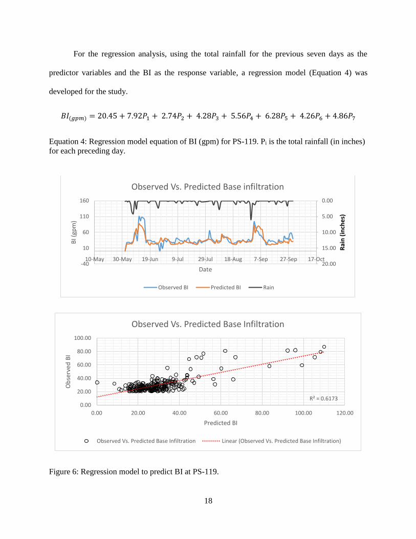
For the regression analysis, using the total rainfall for the previous seven days as the

predictor variables and the BI as the response variable, a regression model (Equation 4) was

developed for the study.

𝐵𝐼(𝑔𝑝𝑚) = 20.45 + 7.92𝑃1 + 2.74𝑃2 + 4.28𝑃3 + 5.56𝑃4 + 6.28𝑃5 + 4.26𝑃6 + 4.86𝑃7

Equation 4: Regression model equation of BI (gpm) for PS-119. Pi is the total rainfall (in inches)

for each preceding day.

Figure 6: Regression model to predict BI at PS-119.

0.00

5.00

10.00

15.00

20.00-40

10

60

110

160

10-May 30-May 19-Jun 9-Jul 29-Jul 18-Aug 7-Sep 27-Sep 17-Oct

Rai

n (

inch

es)

BI (

gpm

)

Date

Observed Vs. Predicted Base infiltration

Observed BI Predicted BI Rain

R² = 0.61730.00

20.00

40.00

60.00

80.00

100.00

0.00 20.00 40.00 60.00 80.00 100.00 120.00

Ob

serv

ed B

I

Predicted BI

Observed Vs. Predicted Base Infiltration

Observed Vs. Predicted Base Infiltration Linear (Observed Vs. Predicted Base Infiltration)

19

From the regression model, the coefficients for rainfall on day 1, 4 and 5 are greater than

the coefficients of other days, thus showing a strong correlation of the rainfall event on the BI.

The R-squared value for this regression model is 0.62, which is considered satisfactory for the

model due to the complexity of the system’s response to different rainfall patterns, for different

events and the complexity of cracks geometry in the sewer network (Figure 6)

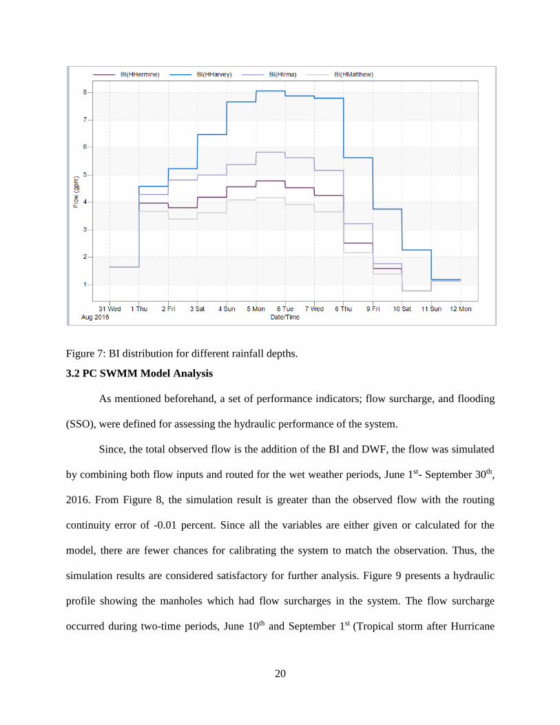
As previously mentioned the regression model is used to predict the BI for different

rainfall events including hurricane events and routed through the system to analyze the hydraulic

performance of the system. For hurricane events, the rainfall was spiked up with the period of the

hurricane and sewer flows were routed for the following days to observe how the system reacts

to the events. Table 1 and Figure 7 below shows different rainfall depths and BI distribution

respectively, corresponding to different hurricane events used for the analysis

Table 1: Different rainfall depths for different hurricane events.

Hurricane events Date Total rainfall depths

Hurricane Matthew August 28th - September 3rd, 2016 14 inches

Hurricane Hermine September 28th - October 1st ,2016 17 inches

Hurricane Irma September 10th - September 12th, 2017 22 inches

Hurricane Harvey August 30th - September 1st, 2017 38 inches

20

Figure 7: BI distribution for different rainfall depths.

3.2 PC SWMM Model Analysis

As mentioned beforehand, a set of performance indicators; flow surcharge, and flooding

(SSO), were defined for assessing the hydraulic performance of the system.

Since, the total observed flow is the addition of the BI and DWF, the flow was simulated

by combining both flow inputs and routed for the wet weather periods, June 1st- September 30th,

2016. From Figure 8, the simulation result is greater than the observed flow with the routing

continuity error of -0.01 percent. Since all the variables are either given or calculated for the

model, there are fewer chances for calibrating the system to match the observation. Thus, the

simulation results are considered satisfactory for further analysis. Figure 9 presents a hydraulic

profile showing the manholes which had flow surcharges in the system. The flow surcharge

occurred during two-time periods, June 10th and September 1st (Tropical storm after Hurricane

21

Hermine), and lasted for about 96 hours after these events. The total rainfall of the seven

previous days for the two events were greater than 10 inches.

Figure 8: PS-119 simulated time series graph, DWF+BI from June–September 2016. C32 = Q

sim, PS-119 = observed flow

Figure 9a: Hydraulic profile of flow surcharge downstream on June 10th. Total rainfall = 11.49

inches

Ground surface

22

Figure 9b: Hydraulic profile of flow surcharge downstream on September 1st. Total rainfall =

10.46 inches

Using the regression model, and increasing the rainfall exceeding 11 inches, the

performance indicators regarding SSO (flooding) and surcharge and their values are presented in

Table 1. The performance indicators show that as rainfall depth increases, the hydraulic grade

line, the number of manholes and hours the manholes stayed surcharged increases (Figure 9).

More so, it is intuitive that the longest surcharge manholes are located downstream of the

system, since that is the location where all the flow converges before flowing into the wet well,

PS-119. Additionally, looking at the pipe slopes, the slopes of the downstream pipes are mild,

almost horizontal, thus increasing the potential for the flow to go from gravity to pressurized

flow. Although the number and the length of time of surcharged manholes increased, there was

no SSO at the manhole. Thus, the existing sewer system is most reliable and less vulnerable to

Ground surface

23

SSO. However, as mentioned in the introduction, SSO can occur at the wet well, and in this

study case at the lift station, PS-119.

Since the capacity of PS-119 is unknown, PS-119 capacity (in gpm) was calculated using

the number of houses, the average household sewer flow, and the peaking factor. As mentioned

beforehand, the area of the sewershed is about 72 acres, and assuming each house is about one-

quarter acre, the average household sewer flow is 300 GPD, peaking factor is 3 and the roads and

curbs are about 11 acres, the lift station capacity is approximately 200 gpm (equation 5)

𝑃𝑆 − 119 𝑐𝑎𝑝𝑎𝑐𝑖𝑡𝑦 = ((72 − 11)

0.25) ∗ (300 𝐺𝑃𝐷) ∗ (

1

1440) ∗ 3

Equation 5: Lift station (PS-119) design capacity

Furthermore, SSO occurred at the wet well, PS-119 (Figure 10), where the total flow

received exceeds the calculated capacity at PS-119. Figure 10 shows the flow hydrographs of the

different rainfall depths and the observed sewer flow compared to the PS-119 flow capacity.

From the hydrographs and from Table 2, it shows that as the rainfall depths increase, the volume

(area under the curve) of SSO at the lift station increases. Thus, the existing lift station, PS-119,

is less reliable and more vulnerable to SSO.

Table 2: Sewer system hydraulic performance indicators for different rainfall depths.

Performan

ce

indicators

Details Rainfall depths

Matthe

w

Hermi

ne

Irma 25-

inches

30-

inches

Harve

y

40-

inches

Manhole

surcharge

Number of

surcharged

manholes

10

manho

les

14

manho

les

15

manho

les

17

manho

les

17

manho

les

20

manho

les

21

manhol

es

Manhole

with

maximum

hours

surcharged

SM

2006

(188.8

7 hrs.)

SM

2006

(198.4

7 hrs.)

SM

2006

(207.7

9 hrs.)

SM

2006

(211.6

9 hrs.)

SM

2006

(220.2

1 hrs.)

SM

2006

(238.1

4 hrs.)

SM

2006

(245.7

5 hrs.)

PS-119

SSO

Total

volume of

SSO

24,833 43,850 74,344 83,321 116,31

2

148,51

2

172,89

5

24

Figure 10a: Hurricane Harvey rainfall depth. Hydraulic profile plot showing surcharged

manholes

Figure 10b: 40-inches rainfall depth. Hydraulic profile plot showing surcharge manholes

Ground surface

Ground surface

25

Figure 11: Flow hydrographs of the different rainfalls depths vs. PS-119 design capacity

0

100

200

300

400

500

600

8/30 9/1 9/3 9/5 9/7 9/9 9/11 9/13 9/15

Flo

w (

gpm

)

Date

Simulated flow Vs. PS-119 Flow Capacity

HHarvey HHermine HIrma

HMatthew PS-119 Capacity Observed flow

26

CHAPTER 4: CONCLUSION

Sanitary sewer overflow releases harmful contaminants, pollutants and nutrients that are

detrimental to the environment, ecosystem and public health, and more so poses a financial

difficulty to clean out the effects both on the environment and the public. In this study,

performance indicators were defined to help evaluate the hydraulic performance of the existing

system. Since the PS-119 sewer is located on an area with shallow water table (ranging from 2 to

6 ft. below the ground elevation), groundwater infiltration would be a major problem, in addition

to blockages and debris build up, thereby reducing the pipe diameter, will lead to flow surcharge

and SSO.

The time series analysis ruled out surface inflow as a significant source of freshwater

contribution to excess sewer flow. Using the Steven-Schutzbach method, the base infiltration

calculation showed that an annual of 49% of the flow during the wet weather, and 42% during

dry weather was essentially groundwater infiltration. Thus, presenting a challenge of high

infiltration into the sewer system. Correlation analysis suggests that significant relationship for 7

days between base infiltration and rainfall. The analysis suggests that the rainfall takes about 1-2

days to infiltrate the soil and raise the water table, peaking on day 4 and receding from day 5 to

day 7 after the rainfall event. Applied to regression analysis to predict future base infiltration for

different rainfall depths, it further showed the increase in the base infiltration flow as the rainfall

depths increases.

27

Comparing the results of the hydraulic performance for different rainfall depths, showed

that as the rainfall depths increase, the number and hours the surcharged manholes increases but

no SSO occurred at the manholes. SSO occurred at the wet well, PS-119, and as the rainfall

depths increased, the volume of SSO increased. However, since the occurrences of such high

rainfall depths for SSO are rare, the system is considered reliable and less vulnerable.

Furthermore, carefully looking at the surcharge manholes, the locations of the manholes are

downstream of the system, where all the flow converges, and the pipe slopes are relatively

horizontal. The observation helps pinpoint crucial locations where system failure is more likely

to occur and can help propose a more strategic, sustainable, cost-effective plan to mitigate the

negative impacts of sanitary sewer overflows.

In conclusion, the hydraulic performance study helps provide information for strategic

planning, implementing and improving the existing sanitary system to reduced rainfall-induced

overflows. Future studies will detail the impacts of rehabilitation on the reduction of the

infiltration in the system. This study will serve as a primary hydraulic model for the future study

and will help compare and analyze the results, before and after rehabilitation.

28

LIST OF REFERENCES

CHI PC SWMM 2017. Avaiable online https://www.pcswmm.com/. (accessed on April 2018)

Environmental Protection Agency, (EPA) (1995). "An Introduction to Sanitary Sewer

Overflow."

Environmental Protection Agency, (EPA) (2004) “Human Health Impacts of CSOs and SSOs”.

2004 Report to congress. Retrieved from

https://www.epa.gov/sites/production/files/2015-

10/documents/csossortc2004_chapter06.pdf

Environmental Protection Agency, (EPA) (2008). "Review of Sewer Design Criteria and RDII

Prediction Methods" Report number EPA/600/R-08/010

Environmental Protection Agency (EPA) (2017), "Storm Water Management Model Reference

Manual Volume II-Hydraulic", Office of Research and Development. National Risk

Management Laboratory Retrieved from

https://nepis.epa.gov/Exe/ZyPDF.cgi/P100S9AS.PDF?Dockey=P100S9AS.PDF

Environmental Protection Agency (EPA), (2016), "Storm Water Management Model Reference

Manual Volume I-Hydrology (Revised)”, Office of Research and Development. National

Risk Management Laboratory Retrieved from

https://nepis.epa.gov/Exe/ZyPDF.cgi/P100NYRA.PDF?Dockey=P100NYRA.PDF

Megan E. Long. "Quantify and Modeling Surface Inflow and Groundwater Infiltration into

Sanitary Sewer Systems in Southern Pinellas County, Fl." Thesis Report. 2017.

Mitchell P.S, Stevens P.L and Nazaroff A. "A Comparison of Methods and Simple Empirical

Solutions to Quantifying Base Infiltration in Sewers." Water Practice (2007).

National Hurricane Center (NOAA), "National Hurricane Center Tropical Cyclone Report,

Hurricane Harvey" May 9th, 2018, Retrieved from

https://www.nhc.noaa.gov/data/tcr/AL092017_Harvey.pdf

National Hurricane Center (NOAA), "National Hurricane Center Tropical Cyclone Report,

Hurricane Irma" March 9th, 2018, Retrieved from

https://www.nhc.noaa.gov/data/tcr/AL112017_Irma.pdf

29

National Hurricane Center (NOAA), "National Hurricane Center Tropical Cyclone Report,

Hurricane Hermine" January 30th 2017, 2017, Retrieved from

https://www.nhc.noaa.gov/data/tcr/AL092016_Hermine.pdf

National Hurricane Center (NOAA), "National Hurricane Center Tropical Cyclone Report,

Hurricane Matthew" April 17th, 2017, Retrieved from h

https://www.nhc.noaa.gov/data/tcr/AL142016_Matthew.pdF

Neuhaus L. Sewage Overflow Again Fouls Tampa Bay After Storm. 16 September 2016. The

New York Times.

P Staufer, A. Scheidegger, J Rieckermann. "Assessing the performance of sewer rehabilitation

on the reduction of infiltration and inflow." Water Research (2012).

Petrequin, M. The Crisis in U.S. Wastewater Infrastructure: History, Issue, and Solutions.

Colorado: Colorado School of Mines, Department of Environmental Science and

Engineering, 2013. Retrieved from

http://www.academia.edu/1786909/The_Crisis_in_U.S._Wastewater_Infrastructure.

Petroff, Ralph G. "An Analysis of the Root Cause of Sanitary Sewer Overflows." n.d. ADS

Environmental Services, Inc., Huntsville, Alabama.

Richard Field, M. ASCE and Thoma P. O'Connor, Assoc. M. ASCE. "Control Strategy for

Storm-Generated Sanitary Sewer Overflows."Global Solutions for Urban Drainage

(2002). American Society of Civil Engineers (ASCE).

Tasnim Nasrin, Ashok K.Sharma, and Nitin Muttil. "Impact of Short Duration Intense Rainfall

Events on Sanitary Sewer Network Performance." Water (2017).

Texas Commission on Environmental Quality (TCEQ), "Sanitary Sewer Overflows from

Hurricane Harvey," Retrieved from

https://www.tceq.texas.gov/response/hurricanes/sanitary-sewer-overflows. 2017.

Toni Panaou, Tinusew Asefa, Ph.D., P.E, D.WRE, Mahmood Nachabe, Ph.D. P.E. "Ascertaining

If General Circulation Models Replicate Historic Performance Metrics for Hydrologic

And Systems Simulations." Ph.D. Paper. 2017.

30

APPENDIX A: SUPPLEMENTAL FIGURES

Figure A1: Cross section of surcharged manhole

Figure A2: Cross section of ponded/overflowed manhole

31

Figure A3: Rainfall intensity from February-September 2016

Figure A4: Total observed flow and BI for PS-119.

-50

0

50

100

150

200

250

12/12 1/31 3/21 5/10 6/29 8/18 10/7 11/26

Flo

w (

GP

M)

Date

PS-119 Total observed flow and Base Infiltration

Total observed flow Base Infiltration (BI)

32

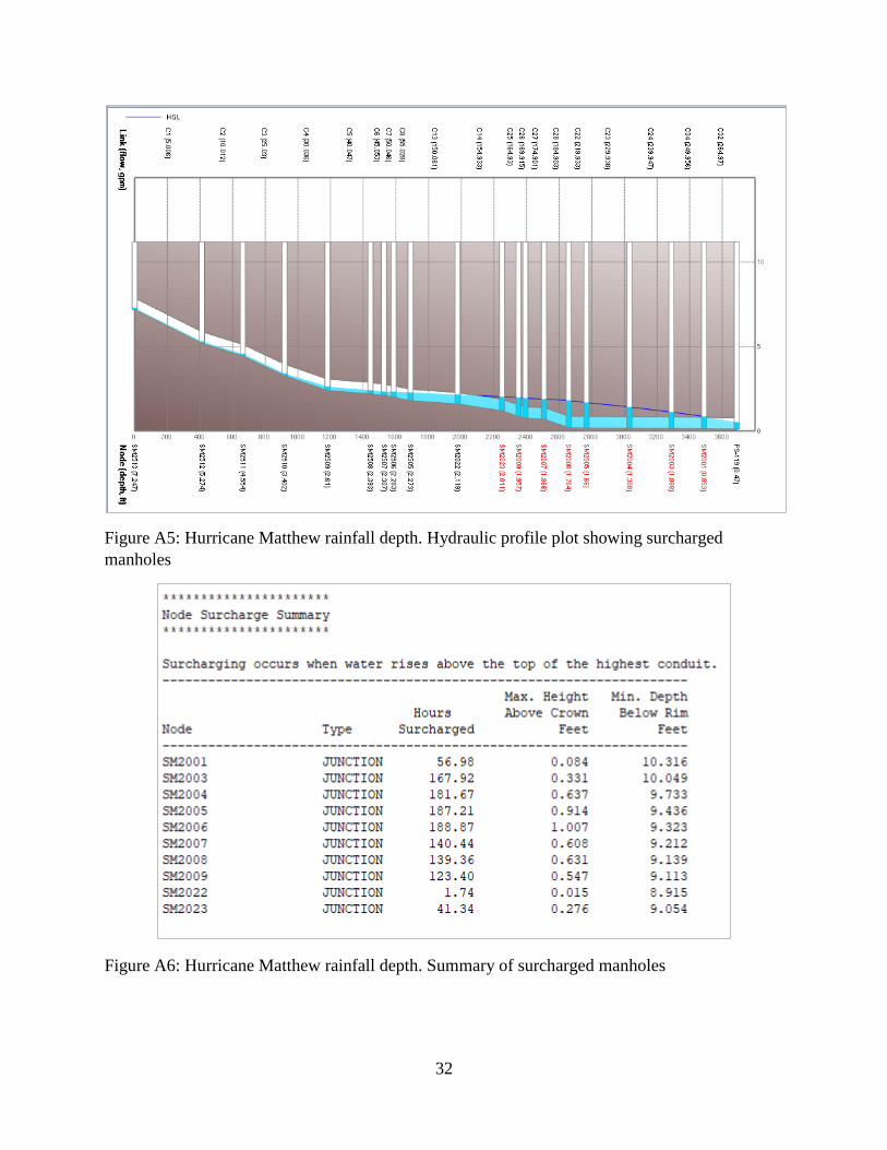
Figure A5: Hurricane Matthew rainfall depth. Hydraulic profile plot showing surcharged

manholes

Figure A6: Hurricane Matthew rainfall depth. Summary of surcharged manholes

33

Figure A7: Hurricane Hermine rainfall depth. Hydraulic profile plot showing locations of

surcharged

Figure A8: Hurricane Hermine rainfall depth. Summary of surcharged manholes

34

Figure A9: Hurricane Irma rainfall depth. Hydraulic profile plot showing locations of surcharged

manholes

Figure A10: Hurricane Irma rainfall depth. Summary of surcharged manholes

35

Figure A11: 25-inches rainfall depth. Hydraulic profile plot showing locations of surcharged

manholes

Figure A12: 25-inches rainfall depth. Summary of surcharged manholes

36

Figure A13: 30-inches rainfall depth. Hydraulic profile plot showing locations of surcharged

manholes

Figure A14: 30-inches rainfall depth. Summary of surcharged manholes

37

Figure A15: Hurricane Harvey rainfall depth. Summary of surcharged manholes

38

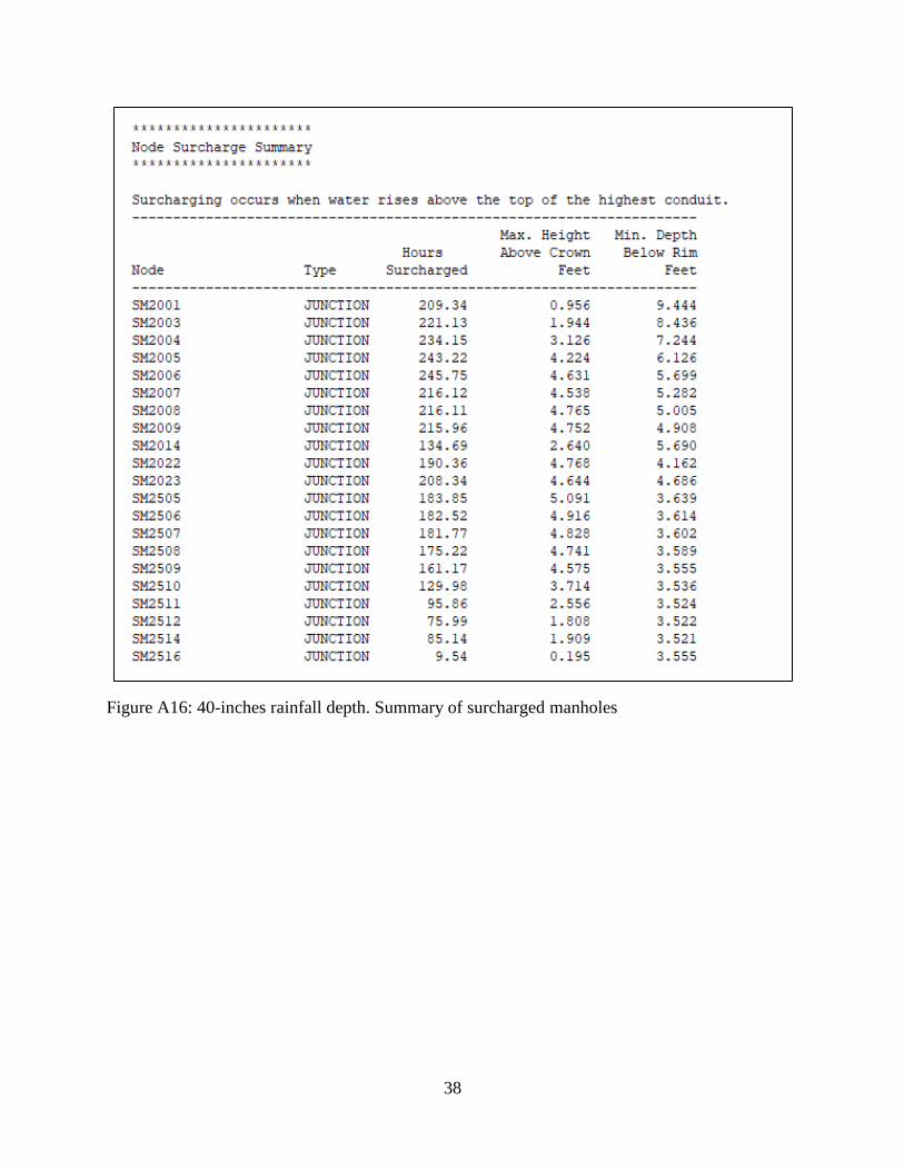
Figure A16: 40-inches rainfall depth. Summary of surcharged manholes