Hydraulic Performance of Bridge Rails (FHWA/TX-09/0 … · • Hydraulic Performance of Bridge Rails based on Rating Curves and Submergence ... 3.2.2 Methodology ... Experiment Results

Technical Report Documentation Page

1. Report No. FHWA/TX-09/0-5492-1

2. Government Accession No.

3. Recipient’s Catalog No.

4. Title and Subtitle Hydraulic Performance of Bridge Rails

5. Report Date October 2008; Revised January 2009

6. Performing Organization Code 7. Author(s)

Randall J. Charbeneau, Brandon Klenzendorf, and Michael E. Barrett

8. Performing Organization Report No. 0-5492-1

9. Performing Organization Name and Address Center for Transportation Research The University of Texas at Austin 3208 Red River, Suite 200 Austin, TX 78705-2650

10. Work Unit No. (TRAIS) 11. Contract or Grant No.

0-5492

12. Sponsoring Agency Name and Address Texas Department of Transportation Research and Technology Implementation Office P.O. Box 5080 Austin, TX 78763-5080

13. Type of Report and Period Covered Technical Report September 2005─August 2008

14. Sponsoring Agency Code

15. Supplementary Notes Project performed in cooperation with the Texas Department of Transportation and the Federal Highway Administration.

16. Abstract This research program addresses issues associated with the hydraulic effects of bridge rails on floodwater levels upstream of bridge structures. The hydraulics of bridge rails and traffic barrier systems are not well understood, especially with regard to rail/barrier systems in series and the submergence of structures. The hydraulics of bridge rails is an important issue for TxDOT bridge rehabilitation projects with potentially significant cost implications. This research project is designed to address issues associated with the hydraulic performance of bridge rails and traffic barriers, and to provide guidance on how different rail/barrier systems can be included in floodplain hydraulics models.

17. Key Words Hydraulics, bridge rails, floodplain, Weir equations, culvert, flow, test channel, return channel, Pitot tube

18. Distribution Statement No restrictions. This document is available to the public through the National Technical Information Service, Springfield, Virginia 22161; www.ntis.gov.

19. Security Classif. (of report) Unclassified

20. Security Classif. (of this page) Unclassified

21. No. of pages 158

22. Price

Form DOT F 1700.7 (8-72) Reproduction of completed page authorized

HYDRAULIC PERFORMANCE OF BRIDGE RAILS Randall J. Charbeneau Brandon Klenzendorf Michael E. Barrett CTR Technical Report: 0-5492-1 Report Date: October 2008; Revised January 2009 Research Project: 0-5492 Research Project Title: Hydraulic Performance of Bridge Rails and Traffic Barriers Sponsoring Agency: Texas Department of Transportation Performing Agency: Center for Transportation Research at The University of Texas at Austin Project performed in cooperation with the Texas Department of Transportation and the Federal Highway Administration.

Center for Transportation Research The University of Texas at Austin 3208 Red River Austin, TX 78705 www.utexas.edu/research/ctr Copyright (c) 2009 Center for Transportation Research The University of Texas at Austin All rights reserved Printed in the United States of America

v

Disclaimers

Authors’ Disclaimer: The contents of this report reflect the views of the authors, who are responsible for the facts and accuracy of the data presented herein. The contents do not necessarily reflect the official view or policies of the Federal Highway Administration or the Texas Department of Transportation. This report does not constitute a standard, specification, or regulation. Patent Disclaimer: There was no invention or discovery conceived or first actually reduced to practice in the course of or under this contract, including any art, method, process, machine manufacture, design or composition of matter, or any new useful improvement thereof, or any variety of plant, which is or may be patentable under the patent laws of the United States of America or any foreign country.

Engineering Disclaimer

NOT INTENDED FOR CONSTRUCTION, BIDDING OR PERMIT PURPOSES

Project Engineer: Randall J. Charbeneau Professional Engineer License Number: Texas No. 56662

P.E. Designation: Research Supervisor

vi

Acknowledgments

The authors would like to express appreciation to David Stolpa (formerly TxDOT) for his initial support of this project. The authors also wish to thank Michael V. Konieczki, Tyler J. McEwen, and Matthew R. Harold for their significant contributions to this research. The following theses were supported through this research program:

• Hydraulic Performance of Bridge Rails based on Rating Curves and Submergence Effects, Joshua Brandon Klenzendorf, M.S. in Engineering, The University of Texas at Austin, May 2007.

• Effects of Bridge Deck Submergence on Backwater, Michael V. Konieczki, M.S. in Engineering, The University of Texas at Austin, May 2007.

• Hydraulic Analysis of Bridge Rails in Series: Rating Curves and Submergence Effects, Tyler J. McEwen, M.S. in Engineering, The University of Texas at Austin, May 2008.

vii

Table of Contents

Chapter 1. Introduction................................................................................................................ 1 1.1 Background and Significance of Work ..................................................................................1 1.2 Study Objectives ....................................................................................................................2 1.3 Overview ................................................................................................................................2

Chapter 2. Background and Literature Review......................................................................... 3 2.1 TxDOT Design Guidance for Bridges ...................................................................................3 2.2 Energy in Open Channel Flow ...............................................................................................5 2.3 Weir Equations ......................................................................................................................7 2.4 Orifice Equation .....................................................................................................................9 2.5 Culvert Performance Curve Model ........................................................................................9 2.6 Weir Submergence Effects Model .......................................................................................11 2.7 Bridge Hydraulics ................................................................................................................14

2.7.1 Flows under the Bridge Decking ................................................................................. 15 2.7.2 Flows over the Bridge Decking ................................................................................... 15 2.7.3 Flows across Bridge Rails ............................................................................................ 15 2.7.4 Effects of Flow Submergence ...................................................................................... 15 2.7.5 Bridge Backwater ......................................................................................................... 16 2.7.6 Bridge Tailwater .......................................................................................................... 16

2.8 Physical Modeling and Scaling ............................................................................................17

Chapter 3. Experimental Programs and Data Models ............................................................ 19 3.1 Hydraulic Performance of Bridge Rails ...............................................................................19

3.1.1 Laboratory Facilities .................................................................................................... 19 3.1.2 Physical Model Construction ....................................................................................... 21 3.1.3 Data Collection Process ............................................................................................... 23 3.1.4 Testing Procedures ....................................................................................................... 29 3.1.5 Bridge Rail Descriptions .............................................................................................. 31 3.1.6 Bridge Rails in Series and Skewed Rail Summary ...................................................... 37

3.2 Hydraulic Performance of Bridge Structure and Rails ........................................................38 3.2.1 Physical Model Description ......................................................................................... 39 3.2.2 Methodology ................................................................................................................ 41

3.3 Data Analysis Models for Bridge Rails ...............................................................................43 3.3.1 Definition of Flow Type .............................................................................................. 43 3.3.2 Rating Curve Model Derivation ................................................................................... 44 3.3.3 Submergence Models ................................................................................................... 47

Chapter 4. Experiment Results and Analysis ........................................................................... 51 4.1 Rating Curve Results ...........................................................................................................51

4.1.1 Observed Data and Analysis of the T203 Rail ............................................................. 51 4.1.2 Model Results .............................................................................................................. 54

4.2 Submergence Effects Results ...............................................................................................61 4.2.1 Observed Data and Analysis of the T203 Data ............................................................ 61 4.2.2 Effects of Rail Submergence........................................................................................ 64 4.2.3 Empirical Model Example ........................................................................................... 65

viii

4.3 Submerged Rating Curve Prediction ...................................................................................67 4.4 Bridge Structure Hydraulics ................................................................................................79

Chapter 5. HEC-RAS Bridge Method Alterations .................................................................. 87 5.1 Bridge Rail Computation Introduction ................................................................................87

5.1.1. High Flow Methods and Selection Overview ......................................................... 88 5.1.2 Energy Method Specifics and Alterations ................................................................... 92 5.1.3 Pressure/Weir Method Specifics and Alterations ........................................................ 94 5.1.4 Discussion .................................................................................................................... 95

5.2 HEC-RAS Model Application to the Simple Bridge Structure ...........................................95 5.3 Weir Coefficient Determination for Use in HEC-RAS Based on Unit Discharge ..............98

5.3.1 Basis for Estimating HEC-RAS Weir Coefficient ....................................................... 99 5.3.2 Example HEC-RAS Application ............................................................................... 100

Chapter 6. Discussion and Conclusions .................................................................................. 103 6.1 Summary of Problem .........................................................................................................103 6.2 Report Objectives and Conclusions ...................................................................................103 6.3 Discussion and Recommendations ....................................................................................104

References .................................................................................................................................. 107

Appendix A: Raw Data ............................................................................................................. 109

ix

List of Figures Figure 2.1: Specific Energy Graph ................................................................................................. 6

Figure 2.2: Sharp-Crested Weir Schematic .................................................................................... 8

Figure 2.3: Submerged Culvert Flow (source: Charbeneau et al., 2006) ..................................... 10

Figure 2.4: Villemonte Model Setup (source: Villemonte, 1947) ................................................ 12

Figure 2.5: Submergence Effects on Sharp-Crested Weirs .......................................................... 14

Figure 2.6: Submergence effects on sharp-crested and broad-crested structures (Villemonte, 1947; Bradley, 1978) ................................................................................... 16

Figure 3.1: CRWR Outdoor Channel Facility .............................................................................. 20

Figure 3.2: Headbox at Upstream End of Test Channel ............................................................... 21

Figure 3.3: Support Base Schematic ............................................................................................. 23

Figure 3.4: Support Base during Construction ............................................................................. 23

Figure 3.5: Pitot Tube Schematic (source: Charbeneau and Holley, 2001) .................................. 24

Figure 3.6: Inclined Manometer Board ......................................................................................... 25

Figure 3.7: Pitot Tube Locations – a) Pitot Tube Spacing Schematic, b) Upstream Pitot Tubes, c) Downstream Pitot Tubes ................................................................................... 26

Figure 3.8: Discharge Weir ........................................................................................................... 27

Figure 3.9: Point Gage .................................................................................................................. 28

Figure 3.10: Tailwater Gate .......................................................................................................... 29

Figure 3.11: T203 Bridge Rail ...................................................................................................... 32



Figure 3.14: SSTR Bridge Rail ..................................................................................................... 34


Figure 3.16: T411 Rail during Construction ................................................................................. 35


Figure 3.18: Model Wyoming Bridge Rails in Series Looking Downstream ............................... 36

Figure 3.19: Weir Rail .................................................................................................................. 37

Figure 3.20: Pitot Tube Locations for Rails in Series ................................................................... 38

Figure 3.21: Skewed T203 Rail .................................................................................................... 38

Figure 3.22: Model bridge deck looking downstream .................................................................. 39

Figure 3.23: Model bridge deck looking upstream ....................................................................... 40

Figure 3.24: Model with two solid railings ................................................................................... 41

Figure 3.25: Model with two 30% open space railings ................................................................ 41

Figure 3.26: Temporary obstruction used to establish an underflow rating curve ....................... 42

Figure 3.27: Flow Type Schematic for T203 Rail ........................................................................ 43

Figure 3.28: Determination of Empirical Parameter, A ................................................................ 48

x

Figure 4.1: Nappe Aeration Stages ............................................................................................... 52

Figure 4.2: Measured T203 Rating Curve Data ............................................................................ 53

Figure 4.3: Calibrated Model Curve for the T203 Rail ................................................................ 54

Figure 4.4: T203 Rating Curve Model .......................................................................................... 55


Figure 4.6: T101D Rating Curve Model ....................................................................................... 56


Figure 4.8: SSTR Rating Curve Model......................................................................................... 57


Figure 4.10: T411 Rating Curve Model ........................................................................................ 58

Figure 4.11: Wyoming Rail Rating Curve Model ........................................................................ 59

Figure 4.12: Weir Rail Rating Curve Model ................................................................................ 59

Figure 4.13: Rail Rating Curve Comparison ................................................................................ 60

Figure 4.14: T203 Submergence Depth Data ............................................................................... 61

Figure 4.15: Submergence Flow Regimes .................................................................................... 62

Figure 4.16: T203 Submergence Model Results ........................................................................... 64

Figure 4.17: Comparison of Submergence Model Standard Error Values between the Villemonte and Empirical Rail Models ............................................................................ 65

Figure 4.18: Bridge Rails in Series ............................................................................................... 67

Figure 4.19: Rating Curves for Upstream (triangle) and Downstream (diamond) Rails in Series for T203 Rail System ............................................................................................. 72



Figure 4.22: Rating Curves for Upstream (triangle) and Downstream (diamond) Rails in Series for Wyoming Rail System ...................................................................................... 75

Figure 4.23: Effects of Downstream Bridge Submergence for T203 Rail ................................... 76



Figure 4.26: Effects of Downstream Bridge Submergence for Wyoming Rail ............................ 78

Figure 4.27: T203 Submergence Model Results for Rails in Series ............................................. 79

Figure 4.28: Rating Curve for Flow beneath the Bridge Structure Decking based on Culvert-Type Flow Analysis with Cb = 0.661 and Cc = 0.933 ......................................... 80

Figure 4.29: Measured Head-Discharge Data for Flow across the Bridge Decking .................... 81

Figure 4.30: Rating Curve for Flow across the Bare Bridge Decking Surface ............................. 82

Figure 4.31: Rating Curve for Flow across Bridge Decking Surface with Solid Rail and Effective Deck Height hDe = hD + hr ................................................................................. 83

Figure 4.32: Rating Curve for Flow across Bridge Decking Surface with Solid Rail and Effective Deck Height hDe = (hD + Mr hr) ......................................................................... 84

xi

Figure 4.33: Rating curve for Flow across Bridge Decking Surface with Open Rail .................. 85

Figure 5.1: Four User-Defined Cross Sections (source: HEC, 2002) ........................................... 87

Figure 5.2: Two Additional RAS-Created Cross Sections (source: HEC, 2002) ......................... 88

Figure 5.3: Upstream End Submerged (Sluice Gate Equation) (source: HEC, 2002) .................. 89

Figure 5.4: Both Ends Submerged (Orifice Equation) (source: HEC, 2002) ............................... 90

Figure 5.5: Upstream End Submerged (Sluice Gate) Coefficient (source: HEC, 2002) .............. 90

Figure 5.6: Pressure Flow and Weir Flow (source: HEC, 2002) .................................................. 91

Figure 5.7: Discharge Reduction Factor based on Percent Submergence (source: HEC, 2002) ................................................................................................................................. 91

Figure 5.8: Energy Equation Parameters (source: HEC, 2002) .................................................... 92

Figure 5.9: Comparison of HEC-RAS Simulation with Measured Data for Simple Bridge Structure with Headboard in Place and Discharge only through the Culvert ................... 96

Figure 5.10: Comparison of HEC-RAS Simulation with Measured Data for Simple Bridge Structure with Discharge through the Culvert and across the Bare Decking Surface .............................................................................................................................. 97

Figure 5.11: Comparison of HEC-RAS Simulation with Measured Data for Simple Bridge Structure with Discharge through the Culvert and across the Decking Surface with Solid Rail ..................................................................................................... 98

Figure 6.1: Example showing debris accumulation at a bridge crossing .................................... 104

Figure 6.2: Contraction coefficient values Cb (cross) and Cc (diamond) as a function of fraction open space for different bridge rails .................................................................. 105

Figure 6.3: Effective flow area as a function of open space for different bridge rails ............... 106

Figure 6.4: Weir-type discharge coefficient Cd as a function of fraction open space ................ 106

xii

xiii

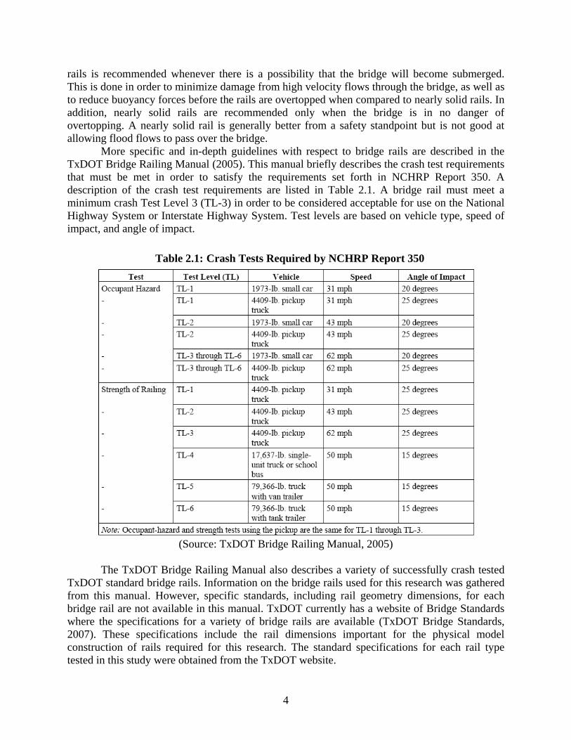
List of Tables Table 2.1: Crash Tests Required by NCHRP Report 350 ............................................................... 4

Table 3.1: Model Rail Dimensions ............................................................................................... 32

Table 4.1: Rating Curve Coefficient Values ................................................................................. 55

Table 4.2: Villemonte and Empirical Submergence Model Parameter Values ............................ 65

Table 4.3: Rating Curve Coefficient Values for Downstream Rail .............................................. 68

Table 4.4: Standard Error for Submergence Models with Rails in Series .................................... 79

xiv

1

Chapter 1. Introduction

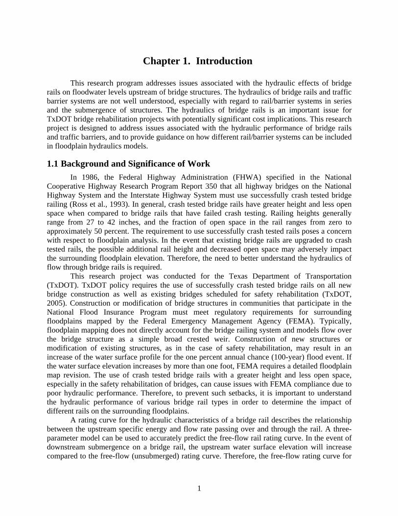
This research program addresses issues associated with the hydraulic effects of bridge rails on floodwater levels upstream of bridge structures. The hydraulics of bridge rails and traffic barrier systems are not well understood, especially with regard to rail/barrier systems in series and the submergence of structures. The hydraulics of bridge rails is an important issue for TxDOT bridge rehabilitation projects with potentially significant cost implications. This research project is designed to address issues associated with the hydraulic performance of bridge rails and traffic barriers, and to provide guidance on how different rail/barrier systems can be included in floodplain hydraulics models.

1.1 Background and Significance of Work In 1986, the Federal Highway Administration (FHWA) specified in the National Cooperative Highway Research Program Report 350 that all highway bridges on the National Highway System and the Interstate Highway System must use successfully crash tested bridge railing (Ross et al., 1993). In general, crash tested bridge rails have greater height and less open space when compared to bridge rails that have failed crash testing. Railing heights generally range from 27 to 42 inches, and the fraction of open space in the rail ranges from zero to approximately 50 percent. The requirement to use successfully crash tested rails poses a concern with respect to floodplain analysis. In the event that existing bridge rails are upgraded to crash tested rails, the possible additional rail height and decreased open space may adversely impact the surrounding floodplain elevation. Therefore, the need to better understand the hydraulics of flow through bridge rails is required. This research project was conducted for the Texas Department of Transportation (TxDOT). TxDOT policy requires the use of successfully crash tested bridge rails on all new bridge construction as well as existing bridges scheduled for safety rehabilitation (TxDOT, 2005). Construction or modification of bridge structures in communities that participate in the National Flood Insurance Program must meet regulatory requirements for surrounding floodplains mapped by the Federal Emergency Management Agency (FEMA). Typically, floodplain mapping does not directly account for the bridge railing system and models flow over the bridge structure as a simple broad crested weir. Construction of new structures or modification of existing structures, as in the case of safety rehabilitation, may result in an increase of the water surface profile for the one percent annual chance (100-year) flood event. If the water surface elevation increases by more than one foot, FEMA requires a detailed floodplain map revision. The use of crash tested bridge rails with a greater height and less open space, especially in the safety rehabilitation of bridges, can cause issues with FEMA compliance due to poor hydraulic performance. Therefore, to prevent such setbacks, it is important to understand the hydraulic performance of various bridge rail types in order to determine the impact of different rails on the surrounding floodplains. A rating curve for the hydraulic characteristics of a bridge rail describes the relationship between the upstream specific energy and flow rate passing over and through the rail. A three-parameter model can be used to accurately predict the free-flow rail rating curve. In the event of downstream submergence on a bridge rail, the upstream water surface elevation will increase compared to the free-flow (unsubmerged) rating curve. Therefore, the free-flow rating curve for

2

a rail will underestimate the upstream water surface elevation when submergence occurs. Analysis of downstream submergence on a bridge rail is characterized using two separate mathematical models in order to determine the additional increase in upstream water surface elevation. These models can then be used together with the free-flow rating curve to develop a submerged rating curve. Hydraulic efficiency is only one important criterion to consider when selecting a bridge rail type. Other important criteria include, but are not limited to, design speed, traffic volume, pedestrian traffic, aesthetics, etc. Therefore, due to the wide range of criteria, nine different bridge rail configurations were analyzed for this research project. Primary testing was conducted as if the rail was on the upstream side of the bridge. Six different standard TxDOT rails were tested: T203, T101, T501, SSTR, T221, and T411. Information on each bridge rail is available on the TxDOT website (TxDOT, 2007) and in the TxDOT Bridge Railing Manual (2005). These rails are also described in Chapter 3 of this report. The T501, SSTR, and T221 are solid rails with a small scupper drain at the bottom but have different cross sectional geometries. The T203 and T411 have an intermediate amount of open space, and the T101 has a large fraction of open space. In addition, the T101 rail was also tested as if on the downstream side of the bridge, labeled as T101D, due to its nonsymmetrical geometry. A solid weir type rail was tested (weir rail), and a two-tube steel railing used in Wyoming (Wyoming rail) was tested due to its large amount of open space (information available online in the FHWA Caltrans Bridge Rail Guide 2005 (FHWA, 2007). Testing was also done with selected rails in series, representing rails on both the upstream and downstream sides of a bridge, and the T203 rail was tested at a skew angle orientation to check orientation effects on the model parameters and rail performance.

1.2 Study Objectives The objectives of the physical hydraulic modeling and analysis research program are 1)

development of rating curves for various solid and open standard TxDOT rails, 2) determination of the hydraulic performance of bridge rail/decking systems, especially with regard to submergence effects, and 3) development of predictive modeling tools for prediction of hydraulic performance of bridge-rail systems in floodplain analysis models such as HEC-RAS.

1.3 Overview Chapter 2 provides the background and literature review for this project. The primary physical modeling experimental program is described in Chapter 3, along with a secondary program to develop a data set on hydraulic performance of an entire bridge system (flow both beneath the bridge decking and across the decking surface). The rating curve model is also developed in Chapter 3. Chapter 4 presents the experimental results and analysis of data. Chapter 5 shows how the results from Chapter 4 can be used with floodplain analysis models such as HEC-RAS to assess the hydraulic effects of different bridge rails. Chapter 6 provides a summary and discussion of the research results.

3

Chapter 2. Background and Literature Review

The literature directly related to the hydraulic performance of bridge rails is very limited. Bridge rails are usually considered a part of the bridge decking. Therefore, in hydraulic equations associated with water flow over a bridge, the actual roadway elevation of the bridge deck is slightly increased to account for the hydraulics of the bridge rails. Typical modeling of water flow over the top of the bridge considers the bridge structure as a broad-crested weir with critical depth near the bridge centerline (Hamill, 1999). Although this is a well accepted method, it is not entirely accurate and can create concerns when small changes in water depth are created due to altering the bridge rails. Therefore, there is a need for a more accurate description of bridge rail hydraulics. In order to accomplish this, literature available on weir type flow and similar structures that can be used to approximate flow over bridge rails is reviewed. This literature, along with the applicable principles of fluid mechanics, is summarized in order to create a basis for the mathematical models used in this research. These models are based on original ideas presented in the literature and are also reviewed here.

2.1 TxDOT Design Guidance for Bridges The Texas Department of Transportation (TxDOT) provides guidance and recommends procedures for the design and construction of a varying range of drainage facilities. These are described in the TxDOT Hydraulic Design Manual (2004). There are several items of particular interest for this research in the Hydraulic Design Manual. The first is the recommended design frequencies for various structures. The design frequency refers to the maximum severity of storm that the structure will pass without inundation. The magnitude of flow associated with each frequency is determined based on historic hydrologic data specific to the area where the structure is located. A freeway bridge structure would most likely be a part of the National Highway System or Interstate Highway System, and would, therefore, be required to have crash tested bridge rails according to NCHRP Report 350 as described in Chapter 1. The recommended design storm for a freeway bridge is a 50-year storm which has a 2% probability of occurrence in any given year. The structure must be checked for a 100-year storm, which has a 1% probability of occurring in any given year. However, the structure is not required to allow all the flood waters to pass under the bridge for this level of a storm. Therefore, in the event of a 100-year storm, a freeway bridge would most likely be overtopped by flood waters, which would force water to flow over the bridge rails and bridge deck roadway. If this occurs, the type of bridge rails would impact the 100-year floodplain associated with the 100-year storm. Such an impact would raise compliance issues with FEMA floodplain maps if the existing bridge rails were upgraded for safety rehabilitation as described in Chapter 1. This reinforces the need to better understand the hydraulic performance of crash tested bridge rails. The recommended design frequency for small bridges on principal arterials and minor arterials and collector roadways is the 25-year storm with a 4% probability of occurrence in any given year. These structures must also be checked for the 100-year storm. Although the TxDOT Hydraulic Design Manual typically discusses the entire bridge structure, it does mention bridge rails specifically on a number of occasions. The Hydraulic Design Manual requires that whenever “higher or less hydraulically efficient railing” is used, the floodplains must be checked for communities participating in the NFIP. The use of open bridge

4

rails is recommended whenever there is a possibility that the bridge will become submerged. This is done in order to minimize damage from high velocity flows through the bridge, as well as to reduce buoyancy forces before the rails are overtopped when compared to nearly solid rails. In addition, nearly solid rails are recommended only when the bridge is in no danger of overtopping. A nearly solid rail is generally better from a safety standpoint but is not good at allowing flood flows to pass over the bridge. More specific and in-depth guidelines with respect to bridge rails are described in the TxDOT Bridge Railing Manual (2005). This manual briefly describes the crash test requirements that must be met in order to satisfy the requirements set forth in NCHRP Report 350. A description of the crash test requirements are listed in Table 2.1. A bridge rail must meet a minimum crash Test Level 3 (TL-3) in order to be considered acceptable for use on the National Highway System or Interstate Highway System. Test levels are based on vehicle type, speed of impact, and angle of impact.

Table 2.1: Crash Tests Required by NCHRP Report 350

(Source: TxDOT Bridge Railing Manual, 2005)

The TxDOT Bridge Railing Manual also describes a variety of successfully crash tested TxDOT standard bridge rails. Information on the bridge rails used for this research was gathered from this manual. However, specific standards, including rail geometry dimensions, for each bridge rail are not available in this manual. TxDOT currently has a website of Bridge Standards where the specifications for a variety of bridge rails are available (TxDOT Bridge Standards, 2007). These specifications include the rail dimensions important for the physical model construction of rails required for this research. The standard specifications for each rail type tested in this study were obtained from the TxDOT website.

5

2.2 Energy in Open Channel Flow For the purposes of this research, testing was conducted in an open channel to simulate water flow in a river or creek. Open channel flow occurs when there is a free surface of fluid that is subject to atmospheric pressure. This type of flow allows for simplification in several governing equations when the atmospheric gage pressure is assumed to be zero. This removes the pressure head term in the energy equation described below. The steady state energy equation describes the energy head at two locations within an open channel (Chow, 1959). This form of the energy equation is normalized to the unit weight of the fluid. Therefore, the terms shown in Equation (2.1) below all have dimensions of length and represent the energy head due to various forces. This form of the energy equation is also known as Bernoulli’s Equation when head losses are negligible.

Lhg

vhz

gv

hz +++=++22

22

222

21

111 αα (2.1)

In Equation (2.1), z is the vertical distance from a constant datum to the channel bottom, h is the water depth, v is the water velocity, α is a kinetic energy coefficient that accounts for a non-uniform flow distribution, hL is a head loss term that occurs due to friction along the channel length and due to channel expansions or contractions between location 1 (upstream) and location 2 (downstream), and g is the gravitational acceleration constant. The specific energy in a channel section is defined as the energy per unit weight of water at any section of a channel, measured with respect to the channel bottom (Chow, 1959). If the velocity is uniform and channel slope is small, then the specific energy is expressed according to Equation (2.2), where Q is the channel discharge (volumetric flow rate) and A is the flow cross-section area.

2

22

22 gAQh

gvhE +=+= (2.2)

If the channel cross section is rectangular, one may define the unit flow rate, q, as the volumetric flow rate per unit width of the channel (b).

vhb

vbhb

vAbQq ==== (2.3)

Equation (2.3) allows the specific energy to be expressed as follows:

2

2

2ghqhE += (2.4)

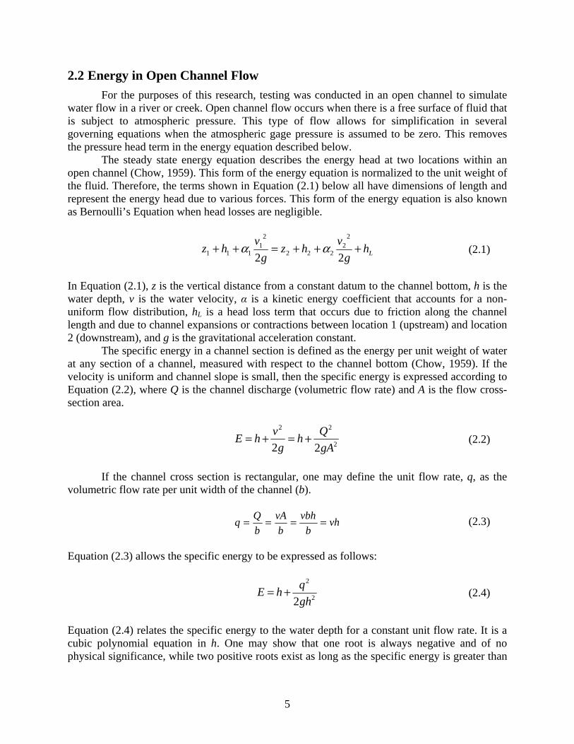
Equation (2.4) relates the specific energy to the water depth for a constant unit flow rate. It is a cubic polynomial equation in h. One may show that one root is always negative and of no physical significance, while two positive roots exist as long as the specific energy is greater than

6

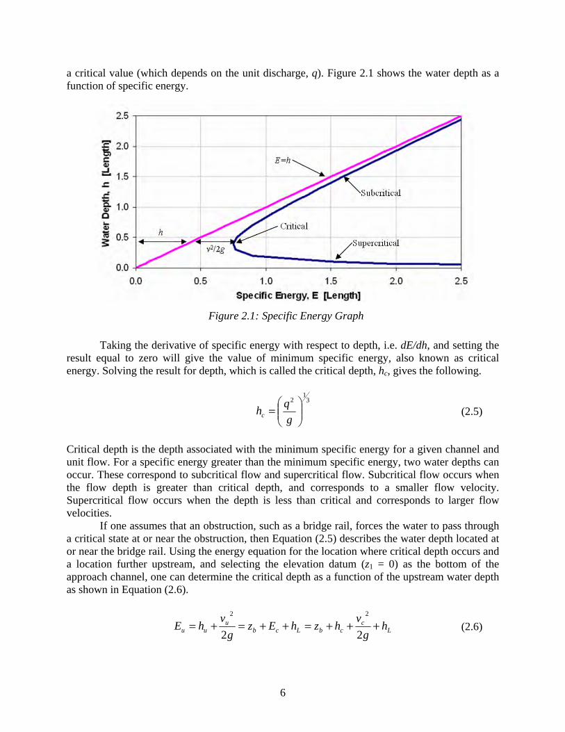
a critical value (which depends on the unit discharge, q). Figure 2.1 shows the water depth as a function of specific energy.

Figure 2.1: Specific Energy Graph

Taking the derivative of specific energy with respect to depth, i.e. dE/dh, and setting the result equal to zero will give the value of minimum specific energy, also known as critical energy. Solving the result for depth, which is called the critical depth, hc, gives the following.

3

12

⎟⎟⎠

⎞⎜⎜⎝

⎛=

gqhc (2.5)

Critical depth is the depth associated with the minimum specific energy for a given channel and unit flow. For a specific energy greater than the minimum specific energy, two water depths can occur. These correspond to subcritical flow and supercritical flow. Subcritical flow occurs when the flow depth is greater than critical depth, and corresponds to a smaller flow velocity. Supercritical flow occurs when the depth is less than critical and corresponds to larger flow velocities. If one assumes that an obstruction, such as a bridge rail, forces the water to pass through a critical state at or near the obstruction, then Equation (2.5) describes the water depth located at or near the bridge rail. Using the energy equation for the location where critical depth occurs and a location further upstream, and selecting the elevation datum (z1 = 0) as the bottom of the approach channel, one can determine the critical depth as a function of the upstream water depth as shown in Equation (2.6).

Lc

cbLcbu

uu hg

vhzhEz

gv

hE +++=++=+=22

22

(2.6)

7

In Equation (2.6) the subscript u refers to the upstream location, the subscript c to the critical flow location near the bridge rail, and zb is the elevation of the bridge decking. Further, we can assume there is no head loss along the length of the channel, i.e. 0≅Lh . In addition, the upstream flow regime will be subcritical due to the obstruction created by the bridge rail so that the upstream water velocity head will be small but not necessarily negligible. Using Equation (2.4), Equation (2.6) can be written as follows.

2

2

2 ccbu gh

qhzE ++= (2.7)

From Equation (2.5), we know that 32

cghq = . Substituting this into Equation (2.7) and rearranging to solve for hc gives the following (Rouse, 1950).

( )buc zEh −=32 (2.8)

Equation (2.8) gives the critical depth as a function of the upstream specific energy and bridge decking elevation. Because we do not know exactly where critical depth occurs, we cannot directly measure this value. However, we can easily measure the upstream water specific energy and use that to calculate the critical depth. This is useful in the derivation of the mathematical model used for approximating the rating curves for each bridge rail type which is described in Chapter 3.

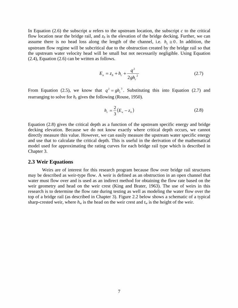
2.3 Weir Equations Weirs are of interest for this research program because flow over bridge rail structures may be described as weir-type flow. A weir is defined as an obstruction in an open channel that water must flow over and is used as an indirect method for obtaining the flow rate based on the weir geometry and head on the weir crest (King and Brater, 1963). The use of weirs in this research is to determine the flow rate during testing as well as modeling the water flow over the top of a bridge rail (as described in Chapter 3). Figure 2.2 below shows a schematic of a typical sharp-crested weir, where hw is the head on the weir crest and tw is the height of the weir.

8

Figure 2.2: Sharp-Crested Weir Schematic

A short distance upstream from the weir, the water velocity is nearly uniform and parallel along the channel. Immediately upstream from the weir, the water at the bottom of the channel must flow upwards in order to pass over the crest of the weir. As the water flows upwards over the weir, it separates from the surface of the weir at the crest and forms a nappe (Rouse, 1950). Air is trapped between the lower surface of the nappe and the downstream face of the weir. If the nappe is not fully aerated, the trapped air will create a negative pressure due to the continual aeration of the flowing water over the weir. If the water flow rate is large enough, the aeration of water will eventually remove virtually all the trapped air under the nappe. In such an event, the nappe will intermittently attach to the downstream face of the weir and result in unstable flow near the weir. This can affect the head measurements taken upstream from the weir and result in inaccurate flow rate values determined by the weir equations described below. The effects of nappe aeration with respect to the results of this research are described in Chapter 4. The general weir equation for weirs with horizontal crests (King and Brater, 1963) is given in the following equation. 5.1

wwbhCQ = (2.9) Q is the volumetric flow rate, hw is the head on the weir crest, Cw is a weir coefficient (dimensional), and b is the length of the weir crest. For a sharp-crested weir, as shown in Figure 2.2, the governing equation is given below according to Rouse (1950).

5.1232

wd hgbCQ = (2.10)

In Equation (2.10) Cd is the dimensionless weir discharge coefficient, and all other parameters have been previously defined. Cd depends on the effects of viscosity, the velocity distribution in the approach section, and capillarity, but it is most easily found by empirical methods (Rouse, 1950). This equation is useful in that one may determine the volumetric flow rate, Q, by simply measuring the head on the weir at an upstream location, assuming one has previously found the

9

correct value of Cd for the weir being used. The sharp-crested weir equation is used in this research for determining the flow rate during testing. Similarly, a broad-crested weir acts in much the same way. Equation (2.11) (Bos, 1989) defines the flow rate over a broad-crested weir.

5.1

32

32

wvd hgbCCQ = (2.11)

Cv is a velocity coefficient that accounts for neglecting the velocity head in the derivation of this equation. This equation is used in the model derivation for the rating curve describing flow over the top of a bridge rail.

2.4 Orifice Equation An orifice is a restricted opening with a closed perimeter through which water flows (King and Brater, 1963). Many of the same principles of fluid mechanics apply to orifices that were described for weirs. The flow rate through a sharp-crested orifice (Bos, 1989) is described in Equation (2.12). ood ghACQ 2= (2.12) Cd is the dimensionless discharge coefficient, Ao is the cross-sectional area of the orifice opening, ho is the upstream head acting on the centroid of the orifice area, and all other parameters have been previously defined. For a submerged orifice, the downstream head affects the flow rate. This is shown in Equation (2.13) (Bos, 1989). ood hgACQ Δ= 2 (2.13)

ohΔ is the difference in upstream and downstream heads on the orifice, i.e., odouo hhh −=Δ , where hou is the upstream orifice head and hod is the downstream orifice head acting on the centroid of the orifice. Orifice flow is useful for approximating water flow through the open space in bridge rails used in the rating curve model and for flow beneath the bridge deck.

2.5 Culvert Performance Curve Model The equations and ideas used to develop the mathematical model for the bridge rail rating curves come from previous research described in Charbeneau et al. (2006). In their research, the hydraulic performance of highway culverts was of concern, but the same ideas can be applied to the hydraulic performance of bridge rails. A summary of the culvert model is presented here. The work done by Charbeneau et al. defines a two parameter model for flow through highway culverts during unsubmerged and submerged inlet control conditions. For culvert flow, unsubmerged flow occurs when the headwater (specific energy), given the symbol HW, is less than the culvert rise or height, D. Submerged flow occurs when the headwater is greater than the culvert rise. This model does not account for additional water flow over the top of the roadway that covers the culvert.

10

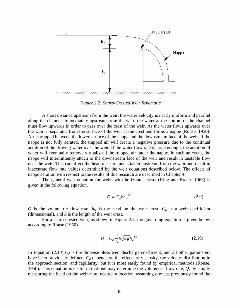
For unsubmerged conditions, the assumption is made that critical flow occurs at or near the culvert entrance and head losses are negligible. Therefore, the specific energy equation can be used to find the headwater depth.

2

21

⎟⎟⎠

⎞⎜⎜⎝

⎛+==

cbc BhC

Qg

hHWE (2.14)

hc is the critical depth at the control section, B is the culvert span or width, Cb is a coefficient expressing the effective horizontal width contraction associated with the culvert entrance edge conditions, and all other parameters have been previously defined. The critical depth, hc, used here is analogous to that defined in Equation (2.8). Making this substitution and rearranging the equation into the form of a performance equation gives the following.

3

23

21

23

⎟⎟⎠

⎞⎜⎜⎝

⎛⎟⎟⎠

⎞⎜⎜⎝

⎛=

gDAQ

CDHW

b

(2.15)

A is the full culvert cross-sectional area, which for a box culvert is A = BD, where D is the culvert rise. For submerged conditions, the culvert may be described as an orifice or sluice gate. The specific energy equation can be used in this case introducing a second contraction coefficient, Cc.

g

vDCHWE en

c 2

2

+== (2.16)

ven is the supercritical velocity at the culvert entrance and Cc is a vertical contraction coefficient associated with flow passing the culvert soffit. Figure 2.3 depicts a physical representation of the parameters used in Equation (2.16).

Figure 2.3: Submerged Culvert Flow (source: Charbeneau et al., 2006)

11

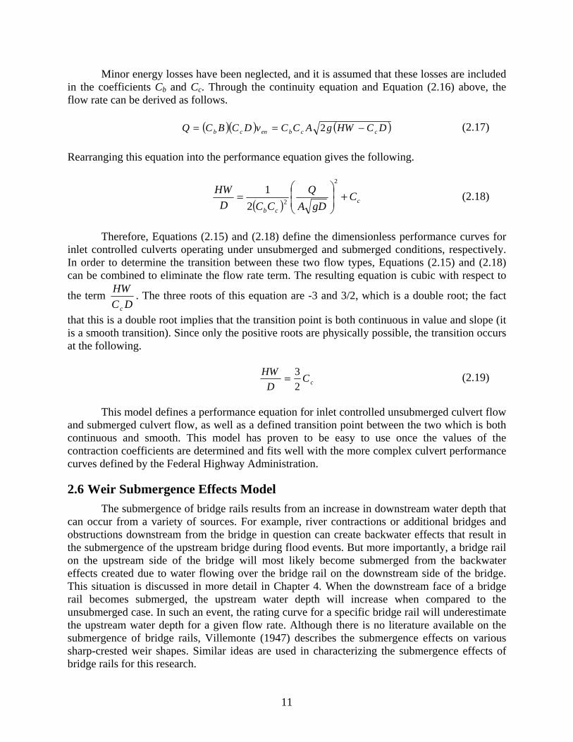
Minor energy losses have been neglected, and it is assumed that these losses are included in the coefficients Cb and Cc. Through the continuity equation and Equation (2.16) above, the flow rate can be derived as follows. ( )( ) ( )DCHWgACCvDCBCQ ccbencb −== 2 (2.17) Rearranging this equation into the performance equation gives the following.

( ) c

cb

CgDA

QCCD

HW +⎟⎟⎠

⎞⎜⎜⎝

⎛=

2

221 (2.18)

Therefore, Equations (2.15) and (2.18) define the dimensionless performance curves for inlet controlled culverts operating under unsubmerged and submerged conditions, respectively. In order to determine the transition between these two flow types, Equations (2.15) and (2.18) can be combined to eliminate the flow rate term. The resulting equation is cubic with respect to

the term DC

HW

c

. The three roots of this equation are -3 and 3/2, which is a double root; the fact

that this is a double root implies that the transition point is both continuous in value and slope (it is a smooth transition). Since only the positive roots are physically possible, the transition occurs at the following.

cCD

HW23= (2.19)

This model defines a performance equation for inlet controlled unsubmerged culvert flow and submerged culvert flow, as well as a defined transition point between the two which is both continuous and smooth. This model has proven to be easy to use once the values of the contraction coefficients are determined and fits well with the more complex culvert performance curves defined by the Federal Highway Administration.

2.6 Weir Submergence Effects Model The submergence of bridge rails results from an increase in downstream water depth that can occur from a variety of sources. For example, river contractions or additional bridges and obstructions downstream from the bridge in question can create backwater effects that result in the submergence of the upstream bridge during flood events. But more importantly, a bridge rail on the upstream side of the bridge will most likely become submerged from the backwater effects created due to water flowing over the bridge rail on the downstream side of the bridge. This situation is discussed in more detail in Chapter 4. When the downstream face of a bridge rail becomes submerged, the upstream water depth will increase when compared to the unsubmerged case. In such an event, the rating curve for a specific bridge rail will underestimate the upstream water depth for a given flow rate. Although there is no literature available on the submergence of bridge rails, Villemonte (1947) describes the submergence effects on various sharp-crested weir shapes. Similar ideas are used in characterizing the submergence effects of bridge rails for this research.

12

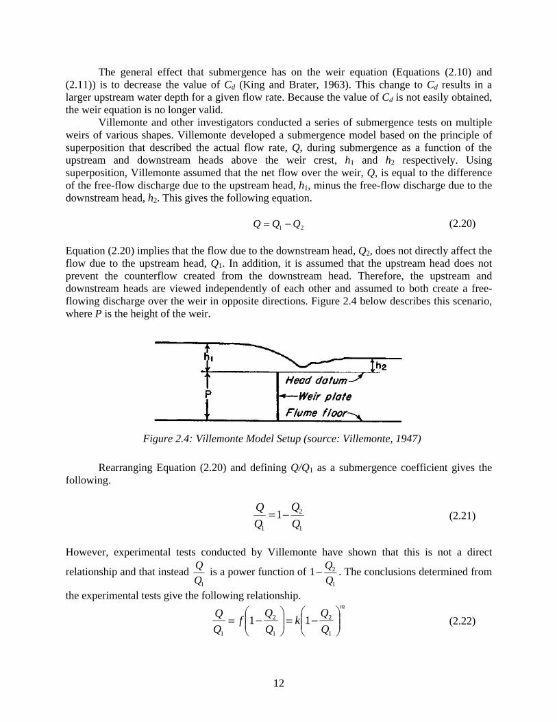
The general effect that submergence has on the weir equation (Equations (2.10) and (2.11)) is to decrease the value of Cd (King and Brater, 1963). This change to Cd results in a larger upstream water depth for a given flow rate. Because the value of Cd is not easily obtained, the weir equation is no longer valid. Villemonte and other investigators conducted a series of submergence tests on multiple weirs of various shapes. Villemonte developed a submergence model based on the principle of superposition that described the actual flow rate, Q, during submergence as a function of the upstream and downstream heads above the weir crest, h1 and h2 respectively. Using superposition, Villemonte assumed that the net flow over the weir, Q, is equal to the difference of the free-flow discharge due to the upstream head, h1, minus the free-flow discharge due to the downstream head, h2. This gives the following equation. 21 QQQ −= (2.20) Equation (2.20) implies that the flow due to the downstream head, Q2, does not directly affect the flow due to the upstream head, Q1. In addition, it is assumed that the upstream head does not prevent the counterflow created from the downstream head. Therefore, the upstream and downstream heads are viewed independently of each other and assumed to both create a free-flowing discharge over the weir in opposite directions. Figure 2.4 below describes this scenario, where P is the height of the weir.

Figure 2.4: Villemonte Model Setup (source: Villemonte, 1947)

Rearranging Equation (2.20) and defining Q/Q1 as a submergence coefficient gives the following.

1

2

1

1QQ

QQ −= (2.21)

However, experimental tests conducted by Villemonte have shown that this is not a direct

relationship and that instead 1Q

Q is a power function of 1

21QQ− . The conclusions determined from

the experimental tests give the following relationship.

m

QQ

kQQ

fQQ

⎟⎟⎠

⎞⎜⎜⎝

⎛−=⎟⎟

⎠

⎞⎜⎜⎝

⎛−=

1

2

1

2

1

11 (2.22)

13

k and m are constants determined empirically from data. Q1 and Q2 can be determined by using the general weir equation shown in Equation (2.9). Representing the power term in Equation (2.9) as the symbol n gives the following.

m

nw

nw

bhCbhC

kQQ

⎟⎟⎠

⎞⎜⎜⎝

⎛−=

1

2

1

1 (2.23)

Villemonte experimentally determined the value of k as 1.00 from results for seven different weir types. Assuming the value of Cw is constant for a given weir geometry gives the following form of the Villemonte equation useful for this research, written in terms of a submergence ratio, h2/h1.

mn

hh

QQ

⎥⎥⎦

⎤

⎢⎢⎣

⎡⎟⎟⎠

⎞⎜⎜⎝

⎛−=

1

2

1

1 (2.24)

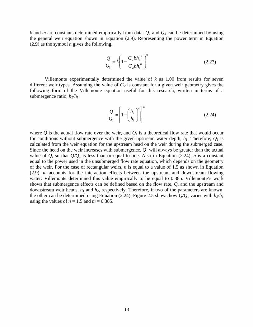
where Q is the actual flow rate over the weir, and Q1 is a theoretical flow rate that would occur for conditions without submergence with the given upstream water depth, h1. Therefore, Q1 is calculated from the weir equation for the upstream head on the weir during the submerged case. Since the head on the weir increases with submergence, Q1 will always be greater than the actual value of Q, so that Q/Q1 is less than or equal to one. Also in Equation (2.24), n is a constant equal to the power used in the unsubmerged flow rate equation, which depends on the geometry of the weir. For the case of rectangular weirs, n is equal to a value of 1.5 as shown in Equation (2.9). m accounts for the interaction effects between the upstream and downstream flowing water. Villemonte determined this value empirically to be equal to 0.385. Villemonte’s work shows that submergence effects can be defined based on the flow rate, Q, and the upstream and downstream weir heads, h1 and h2, respectively. Therefore, if two of the parameters are known, the other can be determined using Equation (2.24). Figure 2.5 shows how Q/Q1 varies with h2/h1 using the values of n = 1.5 and m = 0.385.

14

Figure 2.5: Submergence Effects on Sharp-Crested Weirs

For h2/h1 = 0.0, there is no submergence and Q = Q1. Complete submergence occurs when h2/h1 = 1.0. At this extreme, both h1 and h2 will be very large so that Q1 will also be very large and Q/Q1 will approach zero. Figure 2.5 depicts these two extremes and how the flow varies between the two extremes.

2.7 Bridge Hydraulics Open channel flow hydraulics through bridge structures are outlined by Bradley (1978).

Four distinct flow regimes exist regarding flow through the bridge structure itself: subcritical (Type I) flow, critical (Type II A&B) flow, and supercritical (Type III) flow. Type I flow occurs when the elevation of the water surface remains above the critical depth at all times. Type II flow occurs when the water surface, which was originally higher than critical depth, passes through critical at the bridge structure and then either gradually increases to critical depth, as in Type IIA, or jumps above critical depth as in Type IIB flow. Type III flow occurs when the water surface elevation is below the critical depth at all points.

Each regime has its own set of computational methods for determining backwater based on the energy conservation equation, which take into account the effects of abutment geometry, bridge piers, eccentricity, and skew. Bridge abutment shape is most significant for bridges with a span length less than 200 feet. The significance is proportional to the amount of flow constriction though the bridge structure. Further flow constriction due to bridge piers also increases backwater. Eccentricity occurs when the approach flow on one side of the bridge is less than 20% of that on the other side and results in a slightly higher backwater. Skewed bridges, those that are not perpendicular to the pre-structure flowlines, can themselves both mitigate or increase backwater effects depending on size, abutment shape, and flow constriction (Bradley, 1978).

When flow is sufficiently high, the water surface contacts the upstream face of the bridge resulting in pressurized flow. At this stage the opening beneath the bridge acts as an orifice with

15

flow increasing proportionally to the square root of the upstream head. As the headwater further increases the bridge may be overtopped.

2.7.1 Flows under the Bridge Decking One suggestion for analyzing flow under the bridge decking is to use the standard orifice

head-discharge relationship of Equation (2.12), where ho is the effective head on the orifice. With Z defined as the distance from the lowest bridge girder to the channel bed, the initial value of ho is calculated to the centroid of the flow area (Z/2 for a rectangular orifice). When the orifice is flowing full (submerged), ho is calculated as the relative difference between the upstream and downstream water surface elevations (Δho used in Equation (2.13)). The discharge coefficient is a function of the ratio of the upstream water depth to the bridge height and varies from approximately 0.27 to 0.5. Once the bridge structure is flowing full, however, a constant discharge coefficient of Cd = 0.8 is suggested (Bradley, 1978; HEC, 2002). The limitation of this approach is the assumption that the bridge structure is in fact operating as an orifice.

Another means of analyzing flow under the bridge is to treat the channel opening as a culvert. For flows that are not impinging on the bridge superstructure the head discharge relationship becomes that of a culvert under inlet control, and one set of model equations was presented in Section 2.5. Generally, orifice-type equations are used in mathematical models for floodplain analysis, such as HEC-RAS (HEC, 2002).

2.7.2 Flows over the Bridge Decking Flow that overtops the bridge decking is typically modeled using the head-discharge

relationship for a weir as specified in Equation (2.9). In application to bridge structures, the head on the weir, hw, is the effective head measured from the road crest (highest point of the superstructure). King and Brater (1963) suggest that the point for measuring hw be at a distance of at least 2.5hw upstream of a weir. If the bridge structure and decking are treated as a broad-crested weir, then Bradley (1978) suggests that the weir coefficient Cw falls in the range 3.03 to 3.09 when US Customary units are used. A trapezoidal shape is appropriate for an embankment roadway, but flow over a bridge deck might be more accurately described to be the flow over a rectangular broad-crested weir. HEC (2002) suggests using Equation (2.9) with a weir coefficient of 2.6 US units to calculate the flow over a bridge deck.

2.7.3 Flows across Bridge Rails Currently there is no specific literature on the hydraulics of bridge rails. Bradley (1978)

does not address the issue and HEC-RAS does not allow for the specific input of rail geometry, except for increasing the upper chord elevation to account for the bridge rails (rather than specifying it as the elevation of the road itself).

2.7.4 Effects of Flow Submergence The effects of submergence were described in Section 2.6 for sharp-crested weirs.

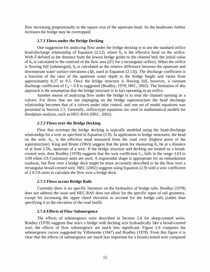
Bradley (1978) suggests that since a bridge with decking acts hydraulically like a broad-crested weir, the effects of flow submergence are much less significant. Figure 2.6 compares the submergence curves suggested by Villemonte (1947) and Bradley (1978). From this figure it is clear that the effects of submergence are much less important for a broad-crested weir compared

16

to a sharp-crested weir. For submergence ratios less than about 0.8, the effects of submergence are negligible for a broad-crested weir.

Figure 2.6: Submergence effects on sharp-crested and broad-crested structures

(Villemonte, 1947; Bradley, 1978)

2.7.5 Bridge Backwater Backwater is the rise in upstream water surface elevation due to the influence of a

hydraulic structure. In general the point at which maximum backwater occurs is at the point just before the flow begins to contract before passing such a structure (Bradley, 1978; HEC 1995). The distance at which the maximum backwater occurs upstream of a bridge generally increases with both the flow rate and bridge width. This point is usually estimated through multiplying the length of the flow obstruction by a contraction coefficient; a ratio of 1:1 is generally used (HEC, 1995). Chapter 5 describes the contraction reach coefficient in greater detail. Bradley (1978) relates the contraction coefficient to the ratio of head difference and normal depth. This method relies heavily on the value of normal depth, and Bradley (1978) offers no general guidelines for determining the contraction reach coefficient.

2.7.6 Bridge Tailwater In order to accurately determine downstream tailwater elevations it is important to

measure the distance after which the flow has completely re-expanded. The length of the expansion reach is determined using a method similar to the one used to calculate the point of maximum backwater, but now an expansion reach coefficient is used. The rule of thumb for the expansion reach coefficient, as suggested by HEC (2002) was considered to be 4:1, but investigations by HEC (1995) have shown that this ratio is generally 1:1 or 2:1. The suggested expansion reach coefficient ranges between 1 and 3.6 depending on flow contraction, bed slope, and Manning’s n coefficient with the higher values associated with larger flows (HEC, 2002). Chapter 5 describes how the expansion reach coefficient is used in hydraulic modeling such as HEC-RAS.

0

0.2

0.4

0.6

0.8

1

0.7 0.75 0.8 0.85 0.9 0.95 1

Submergence Ratio, Hd/Hu

Sub

mer

genc

e C

oeffi

cien

t, C

s

Broad-cres ted (Bradley)

Sharp-cres ted (Villemonte)

17

2.8 Physical Modeling and Scaling Often in hydraulic engineering, physical models are used to study fluid flow phenomenon under controlled laboratory conditions. Proper modeling takes into account modeling relationships designed to create hydraulic similitude between the physical model and its prototype. The prototype is the full-sized object being modeled. Similitude is accomplished through the use of dimensional analysis to insure that certain dimensionless parameters are the same in both the model and prototype. The Froude number is the most significant dimensionless number for open channel models (Warnock, 1950). It is defined in Equation (2.25) below.

gLvFr = (2.25)

Fr is the Froude number, L is a characteristic length, and all other variables have been previously defined. Froude number modeling is used when the inertial forces and gravitational forces are more important than surface tension or viscous forces. This is because the Froude number represents the ratio of inertial forces to gravitational forces. Froude number modeling requires that Frm = Frp, where the subscripts m and p represent the model and prototype, respectively. In addition to hydraulic similitude between the model and prototype, we must maintain constant geometric and kinematic similitude (Warnock, 1950). This is accomplished through the geometric length ratio and velocity ratio, respectively. The length ratio is defined as follows.

p

mr L

LL = (2.26)

where Lr is the length ratio, Lm is the model length scale, and Lp is the prototype length scale. For this research, all length dimensions for individual bridge rails were scaled to half-sized, so that Lr = ½. Since this ratio is maintained for all dimensions, geometric similarity is maintained. To accomplish kinematic similarity, we define a velocity scale ratio.

p

mr v

vV = (2.27)

where Vr is the velocity scale ratio. As previously mentioned, in Froude number modeling, the Froude numbers of the model and prototype are the same, as shown below.

p

p

m

m

gL

v

gLv

= (2.28)

Rearranging Equation (2.28) and solving for the velocity scale ratio gives the following. rr LV = (2.29)

18

Since the volumetric flow rate, Q, is defined as a velocity times an area using the continuity equation, the following flow rate ratio, Qr, can be determined as follows. 2

rrr LVQ = (2.30) Substituting Equation (2.29) into (2.30) gives 2

5rr LQ = (2.31)

Therefore, for the length ratio of ½ used for this research, the corresponding flow rate ratio is equal to ( ) 177.021 2

5==rQ . Through this type of Froude number modeling, various

characteristics and parameters between the model and prototype can be related. In addition to modeling scales, the Froude number can be used to determine when critical depth occurs. As previously mentioned in Section 2.2, critical depth occurs at the minimum specific energy shown in Figure 2.1. When the Froude number is equal to unity, critical depth occurs. When the Froude number is greater than unity, supercritical depth occurs, and when the Froude number is less than unity, subcritical depth occurs. This relationship is useful in the rating curve model derived in Chapter 3.

19

Chapter 3. Experimental Programs and Data Models

The physical modeling program consists of two separate series of investigations using different experimental facilities at the Center for Research in Water Resources (CRWR). The objectives of the first series of investigations were to develop rating curves and characterize the submergence effects in order to determine the hydraulic performance of individual bridge rails, bridge rails in series, and the effects of a skewed alignment between the bridge rail and channel. The objectives of the second series of investigations were to develop a data set for hydraulic performance of a simple bridge system including flow beneath and over the bridge decking that can be used with HEC-RAS in model testing and development. The experimental programs are described in this chapter, and the mathematical model for data analysis is developed.

3.1 Hydraulic Performance of Bridge Rails The objectives of this research program are to apply physical modeling to develop rating curves and characterize the submergence effects in order to determine the hydraulic performance of bridge rails. The bridge rail models were designed and constructed according to the physical model similitude principles and Froude number modeling presented in Section 2.8 and the TxDOT bridge railing standards (TxDOT, 2007). A length scale ratio of Lr = ½ was used for all model bridge rail designs, corresponding to a flow rate ratio of Qr = 0.177 as shown in Section 2.8, and unit flow ratio qr = 0.354. The following sections describe the laboratory facilities available at CRWR to conduct hydraulic testing, as well as specific details regarding the physical model construction and the data collection process. Nine different rail configurations were tested and include the following TxDOT standard bridge rails: T203, T101, T501, SSTR, T221, and T411.

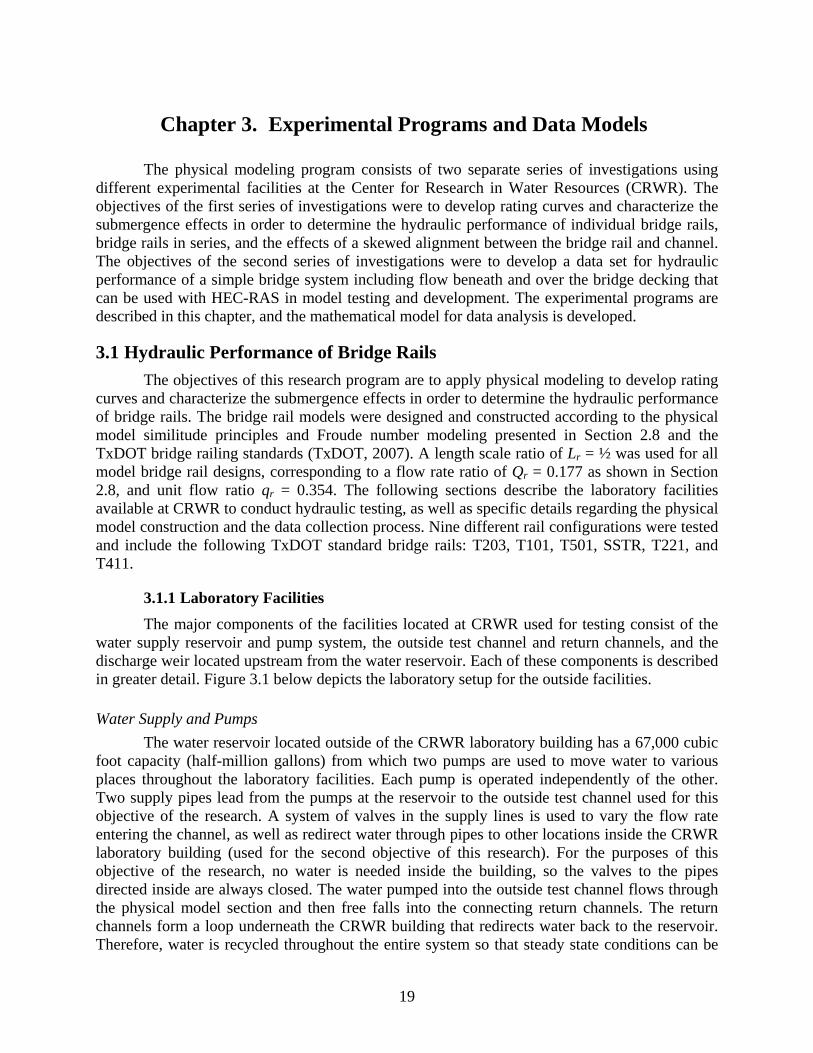
3.1.1 Laboratory Facilities The major components of the facilities located at CRWR used for testing consist of the water supply reservoir and pump system, the outside test channel and return channels, and the discharge weir located upstream from the water reservoir. Each of these components is described in greater detail. Figure 3.1 below depicts the laboratory setup for the outside facilities.

Water Supply and Pumps The water reservoir located outside of the CRWR laboratory building has a 67,000 cubic

foot capacity (half-million gallons) from which two pumps are used to move water to various places throughout the laboratory facilities. Each pump is operated independently of the other. Two supply pipes lead from the pumps at the reservoir to the outside test channel used for this objective of the research. A system of valves in the supply lines is used to vary the flow rate entering the channel, as well as redirect water through pipes to other locations inside the CRWR laboratory building (used for the second objective of this research). For the purposes of this objective of the research, no water is needed inside the building, so the valves to the pipes directed inside are always closed. The water pumped into the outside test channel flows through the physical model section and then free falls into the connecting return channels. The return channels form a loop underneath the CRWR building that redirects water back to the reservoir. Therefore, water is recycled throughout the entire system so that steady state conditions can be

20

met and water is not lost during the testing process. However, there are leaks in the water reservoir which require the occasional addition of water to the system through a pipe receiving water from a nearby water tower on the Pickle Research Campus.

Figure 3.1: CRWR Outdoor Channel Facility

Outside Test Channel and Return Channels The outside test channel is rectangular with a width of 5 feet, a depth of approximately 2

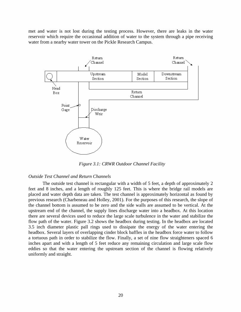
feet and 8 inches, and a length of roughly 125 feet. This is where the bridge rail models are placed and water depth data are taken. The test channel is approximately horizontal as found by previous research (Charbeneau and Holley, 2001). For the purposes of this research, the slope of the channel bottom is assumed to be zero and the side walls are assumed to be vertical. At the upstream end of the channel, the supply lines discharge water into a headbox. At this location there are several devices used to reduce the large scale turbulence in the water and stabilize the flow path of the water. Figure 3.2 shows the headbox during testing. In the headbox are located 3.5 inch diameter plastic pall rings used to dissipate the energy of the water entering the headbox. Several layers of overlapping cinder block baffles in the headbox force water to follow a tortuous path in order to stabilize the flow. Finally, a set of nine flow straighteners spaced 6 inches apart and with a length of 5 feet reduce any remaining circulation and large scale flow eddies so that the water entering the upstream section of the channel is flowing relatively uniformly and straight.

21

Figure 3.2: Headbox at Upstream End of Test Channel

The location and setup of the model bridge rails in the test channel is described in the next section. At the downstream end of the test channel is a tailwater gate that is used to control submergence effects. During data collection for the rail rating curve, this gate is raised out of the water so that it does not impede the flow of water. However, during submergence tests, it is incrementally lowered providing an obstruction for the water as it leaves the channel. As the tailwater gate initially enters the water, it produces a hydraulic jump in the downstream portion of the test channel. When the hydraulic jump reaches the model bridge rail, the rail becomes submerged due to the increased downstream water depth. Immediately downstream from the tailwater gate, the water free falls into the return channels positioned below the test channel. These channels are 3 feet deep and form a loop throughout the entire CRWR laboratory building and back to the reservoir, so that the water used for other experimental setups in the building can be recycled as well. The return channels must reach steady state before accurate flow rate measurements can be taken. Before the water leaves the return channels and reaches the reservoir, it is forced over a sharp-crested discharge weir that is 2 feet high. This is where flow rate measurements are taken by determining the depth, or head, of water flowing over the top of the weir. Measuring the head of water on the weir is accomplished by a point gage device located upstream from the discharge weir. Specific flow rate measurement processes are described in Section 3.1.3. After the water passes over the discharge weir, it returns to the water reservoir.

3.1.2 Physical Model Construction Construction of each model bridge rail was completed according to guidelines set forth by the TxDOT bridge railing standards. Railing standards are currently available online from the TxDOT website (TxDOT Bridge Standards, 2007; http://www.dot.state.tx.us/insdtdot/orgchart/ cmd/cserve/standard/bridge-e.htm). The TxDOT rails that were tested include the T203, T101, T501, SSTR, T221, and T411. All model bridge rails were constructed out of wood, with the exception of the T101 rail which is a combination of wood and metal and the Wyoming rail which is constructed entirely of metal. All dimensions in the railing standards were constructed at a half-sized scale. A half-sized model allowed for the rails to easily fit in the outside test channel at CRWR and still allow a significant height of water to pass over the rail. The 5 foot

22

length of each model bridge rail incorporated all the geometric characteristics of the entire bridge railing system. Therefore, the model rail represents one geometric length of the entire rail. All vertical dimensions were constructed at half-size according to the TxDOT railing standards. However, some slight modifications were made in the horizontal direction to accommodate the channel width restriction and maintain similar values of the percent of open space according to the TxDOT standards. Although these changes in horizontal dimensions might slightly affect the outcome of the rating curves, it is assumed to be more important to maintain the percent open space specified so that sufficient amount of water is allowed to pass through the rail. Finally, where applicable, all chamfers and rounded edges were constructed whenever possible.

Channel Support Base Construction A support base was constructed on the bottom of the test channel so that the force of the flowing water would not push the model bridge rails downstream. The support base and model rails are located roughly 75 feet downstream from the headbox. The support base was made out of wood and concrete. The overall dimensions of the support base used for the testing of single bridge rails are 5 feet along the width of the channel, 4 feet along the length of the channel, and approximately 6.5 inches high. A wooden frame was constructed using several pieces of 2x6 wood and was covered with 5/8 inch plywood to give the top a uniform surface. The 2x6 wood frame does not extend the entire 5 feet in width. Space was left open on either side along the channel walls so that removable 2x6 pieces of wood could be inserted during testing and removed once testing was completed to allow water to drain around the base. This produced some minor leakage through the base during testing but is not considered significant. Modifications to the support base were made for the testing of rails in series and the skewed rail, and details on these modifications are provided in a later section. The inside of the wood frame is divided into two sections. The downstream section was filled with concrete blocks and sand so that air would not become trapped under the support base providing additional buoyancy forces, and the upstream section was filled with concrete. In the upstream section, two steel rods were imbedded in the surrounding wood before pouring the concrete. This allowed the concrete to harden around the rods, which were attached to the wood, preventing the concrete from slipping out of the frame. The concrete was used to increase the weight of the base so it did not float and to bind to the surface of the channel bed so it did not get swept downstream. Three metal pipes, 6 inches in length, were set in the concrete during the construction process and spaced 20 inches apart. These pipes were used to support removable smaller diameter metal pipes that were attached to the model bridge rails. Therefore, the force of flowing water on the rail is transferred to the pipes and into the concrete. Not all of the bridge rails used all three pipes, which is why the support base was designed to accommodate removable pipes whenever they were not needed. Finally, metal anchors were drilled into the concrete channel walls and attached to the wood support base to keep it from being swept downstream. Silicone caulk was used to prevent leaking between the wood and channel bottom and to prevent the sand from washing out of the downstream section. Figure 3.3 depicts the support base constructed in the channel while Figure 3.4 shows the support base during construction.

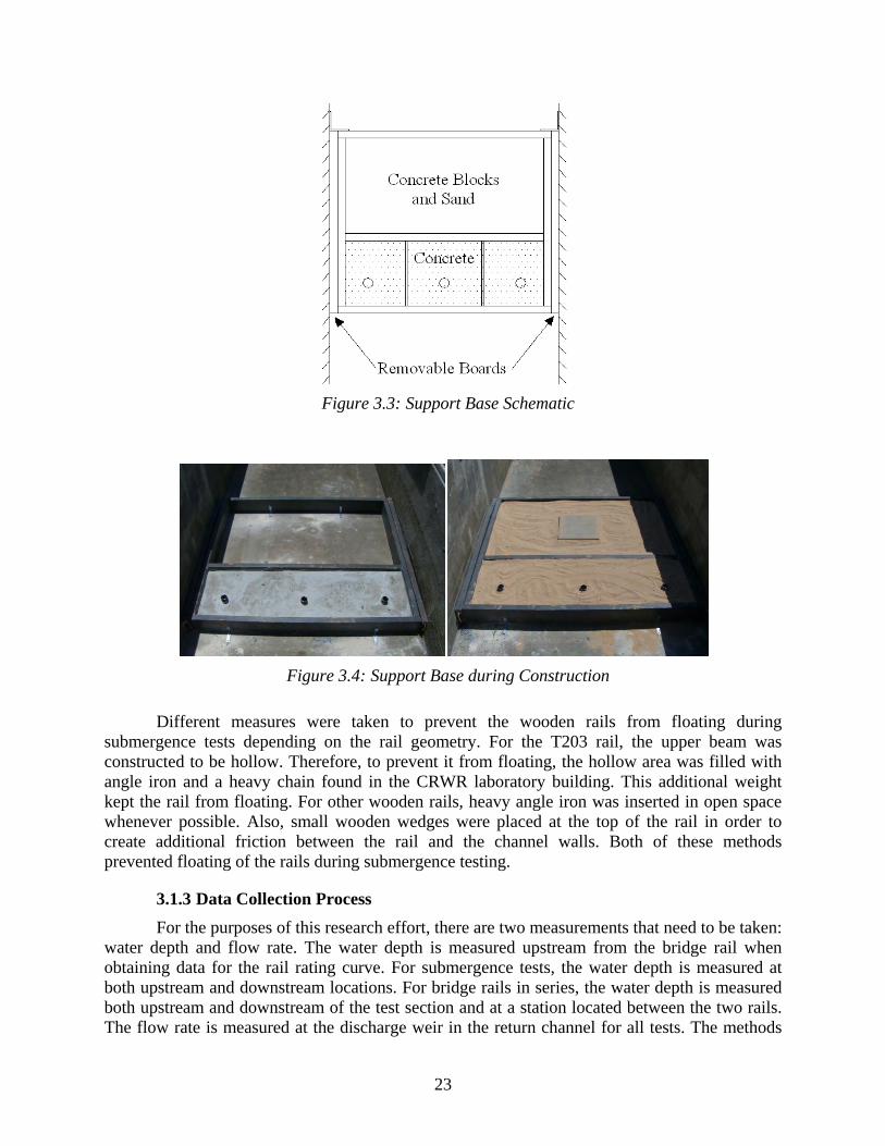
23

Figure 3.3: Support Base Schematic

Figure 3.4: Support Base during Construction

Different measures were taken to prevent the wooden rails from floating during submergence tests depending on the rail geometry. For the T203 rail, the upper beam was constructed to be hollow. Therefore, to prevent it from floating, the hollow area was filled with angle iron and a heavy chain found in the CRWR laboratory building. This additional weight kept the rail from floating. For other wooden rails, heavy angle iron was inserted in open space whenever possible. Also, small wooden wedges were placed at the top of the rail in order to create additional friction between the rail and the channel walls. Both of these methods prevented floating of the rails during submergence testing.

3.1.3 Data Collection Process For the purposes of this research effort, there are two measurements that need to be taken: water depth and flow rate. The water depth is measured upstream from the bridge rail when obtaining data for the rail rating curve. For submergence tests, the water depth is measured at both upstream and downstream locations. For bridge rails in series, the water depth is measured both upstream and downstream of the test section and at a station located between the two rails. The flow rate is measured at the discharge weir in the return channel for all tests. The methods

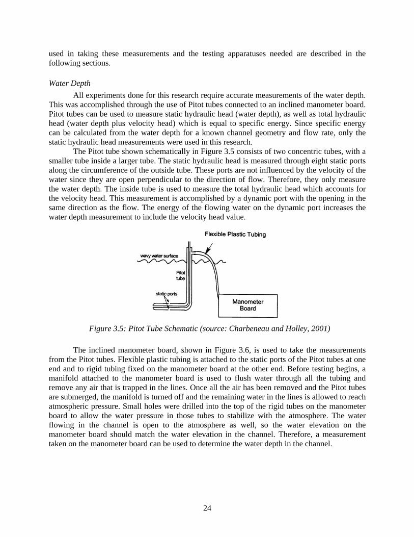
24

used in taking these measurements and the testing apparatuses needed are described in the following sections.

Water Depth All experiments done for this research require accurate measurements of the water depth. This was accomplished through the use of Pitot tubes connected to an inclined manometer board. Pitot tubes can be used to measure static hydraulic head (water depth), as well as total hydraulic head (water depth plus velocity head) which is equal to specific energy. Since specific energy can be calculated from the water depth for a known channel geometry and flow rate, only the static hydraulic head measurements were used in this research. The Pitot tube shown schematically in Figure 3.5 consists of two concentric tubes, with a smaller tube inside a larger tube. The static hydraulic head is measured through eight static ports along the circumference of the outside tube. These ports are not influenced by the velocity of the water since they are open perpendicular to the direction of flow. Therefore, they only measure the water depth. The inside tube is used to measure the total hydraulic head which accounts for the velocity head. This measurement is accomplished by a dynamic port with the opening in the same direction as the flow. The energy of the flowing water on the dynamic port increases the water depth measurement to include the velocity head value.

Figure 3.5: Pitot Tube Schematic (source: Charbeneau and Holley, 2001)

The inclined manometer board, shown in Figure 3.6, is used to take the measurements from the Pitot tubes. Flexible plastic tubing is attached to the static ports of the Pitot tubes at one end and to rigid tubing fixed on the manometer board at the other end. Before testing begins, a manifold attached to the manometer board is used to flush water through all the tubing and remove any air that is trapped in the lines. Once all the air has been removed and the Pitot tubes are submerged, the manifold is turned off and the remaining water in the lines is allowed to reach atmospheric pressure. Small holes were drilled into the top of the rigid tubes on the manometer board to allow the water pressure in those tubes to stabilize with the atmosphere. The water flowing in the channel is open to the atmosphere as well, so the water elevation on the manometer board should match the water elevation in the channel. Therefore, a measurement taken on the manometer board can be used to determine the water depth in the channel.

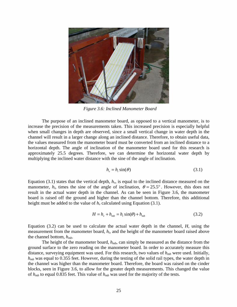
25

Figure 3.6: Inclined Manometer Board

The purpose of an inclined manometer board, as opposed to a vertical manometer, is to increase the precision of the measurements taken. This increased precision is especially helpful when small changes in depth are observed, since a small vertical change in water depth in the channel will result in a larger change along an inclined distance. Therefore, to obtain useful data, the values measured from the manometer board must be converted from an inclined distance to a horizontal depth. The angle of inclination of the manometer board used for this research is approximately 25.5 degrees. Therefore, we can determine the horizontal water depth by multiplying the inclined water distance with the sine of the angle of inclination. )sin(θiv hh = (3.1) Equation (3.1) states that the vertical depth, hv, is equal to the inclined distance measured on the manometer, hi, times the sine of the angle of inclination, °= 5.25θ . However, this does not result in the actual water depth in the channel. As can be seen in Figure 3.6, the manometer board is raised off the ground and higher than the channel bottom. Therefore, this additional height must be added to the value of hv calculated using Equation (3.1). mbimbv hhhhH +=+= )sin(θ (3.2) Equation (3.2) can be used to calculate the actual water depth in the channel, H, using the measurement from the manometer board, hi, and the height of the manometer board raised above the channel bottom, hmb. The height of the manometer board, hmb, can simply be measured as the distance from the ground surface to the zero reading on the manometer board. In order to accurately measure this distance, surveying equipment was used. For this research, two values of hmb were used. Initially, hmb was equal to 0.355 feet. However, during the testing of the solid rail types, the water depth in the channel was higher than the manometer board. Therefore, the board was raised on the cinder blocks, seen in Figure 3.6, to allow for the greater depth measurements. This changed the value of hmb to equal 0.835 feet. This value of hmb was used for the majority of the tests.

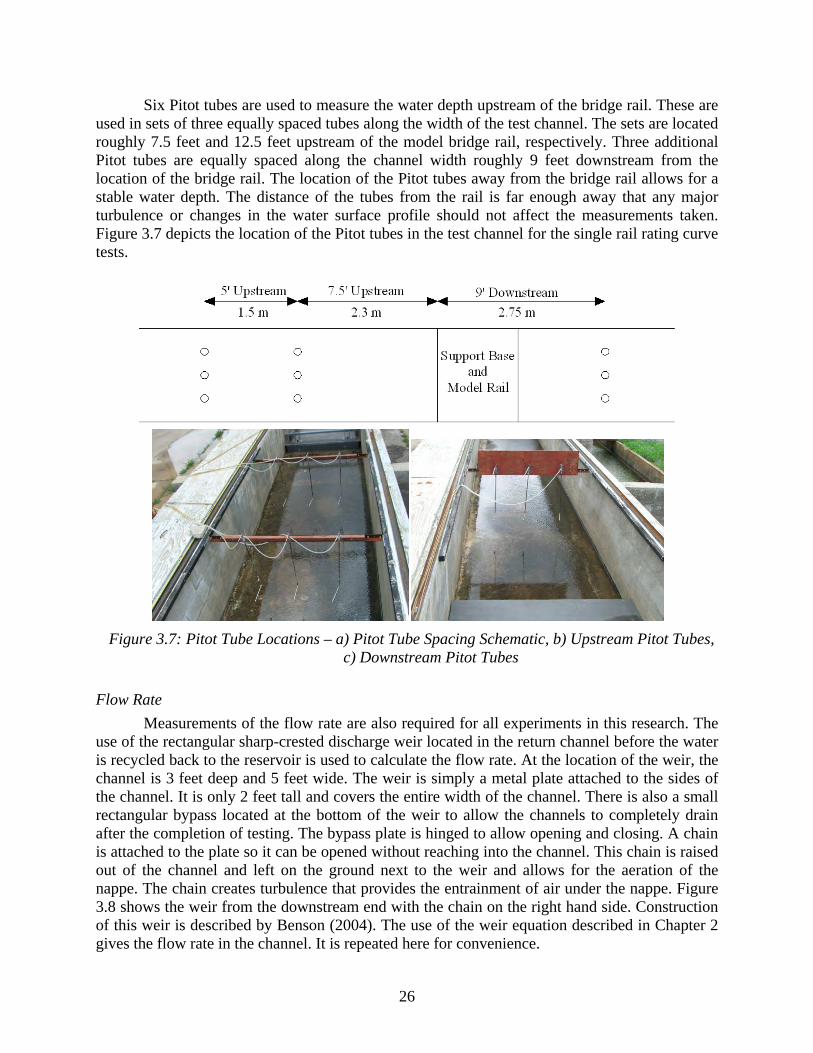
26

Six Pitot tubes are used to measure the water depth upstream of the bridge rail. These are used in sets of three equally spaced tubes along the width of the test channel. The sets are located roughly 7.5 feet and 12.5 feet upstream of the model bridge rail, respectively. Three additional Pitot tubes are equally spaced along the channel width roughly 9 feet downstream from the location of the bridge rail. The location of the Pitot tubes away from the bridge rail allows for a stable water depth. The distance of the tubes from the rail is far enough away that any major turbulence or changes in the water surface profile should not affect the measurements taken. Figure 3.7 depicts the location of the Pitot tubes in the test channel for the single rail rating curve tests.

Figure 3.7: Pitot Tube Locations – a) Pitot Tube Spacing Schematic, b) Upstream Pitot Tubes,

c) Downstream Pitot Tubes

Flow Rate Measurements of the flow rate are also required for all experiments in this research. The use of the rectangular sharp-crested discharge weir located in the return channel before the water is recycled back to the reservoir is used to calculate the flow rate. At the location of the weir, the channel is 3 feet deep and 5 feet wide. The weir is simply a metal plate attached to the sides of the channel. It is only 2 feet tall and covers the entire width of the channel. There is also a small rectangular bypass located at the bottom of the weir to allow the channels to completely drain after the completion of testing. The bypass plate is hinged to allow opening and closing. A chain is attached to the plate so it can be opened without reaching into the channel. This chain is raised out of the channel and left on the ground next to the weir and allows for the aeration of the nappe. The chain creates turbulence that provides the entrainment of air under the nappe. Figure 3.8 shows the weir from the downstream end with the chain on the right hand side. Construction of this weir is described by Benson (2004). The use of the weir equation described in Chapter 2 gives the flow rate in the channel. It is repeated here for convenience.

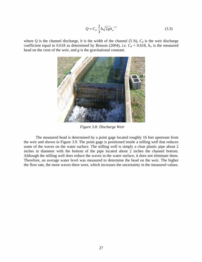
27

5.1232

wd hgbCQ = (3.3)

where Q is the channel discharge, b is the width of the channel (5 ft), Cd is the weir discharge coefficient equal to 0.618 as determined by Benson (2004), i.e. Cd = 0.618, hw is the measured head on the crest of the weir, and g is the gravitational constant.

Figure 3.8: Discharge Weir

The measured head is determined by a point gage located roughly 16 feet upstream from the weir and shown in Figure 3.9. The point gage is positioned inside a stilling well that reduces some of the waves on the water surface. The stilling well is simply a clear plastic pipe about 2 inches in diameter with the bottom of the pipe located about 2 inches the channel bottom. Although the stilling well does reduce the waves in the water surface, it does not eliminate them. Therefore, an average water level was measured to determine the head on the weir. The higher the flow rate, the more waves there were, which increases the uncertainty in the measured values.

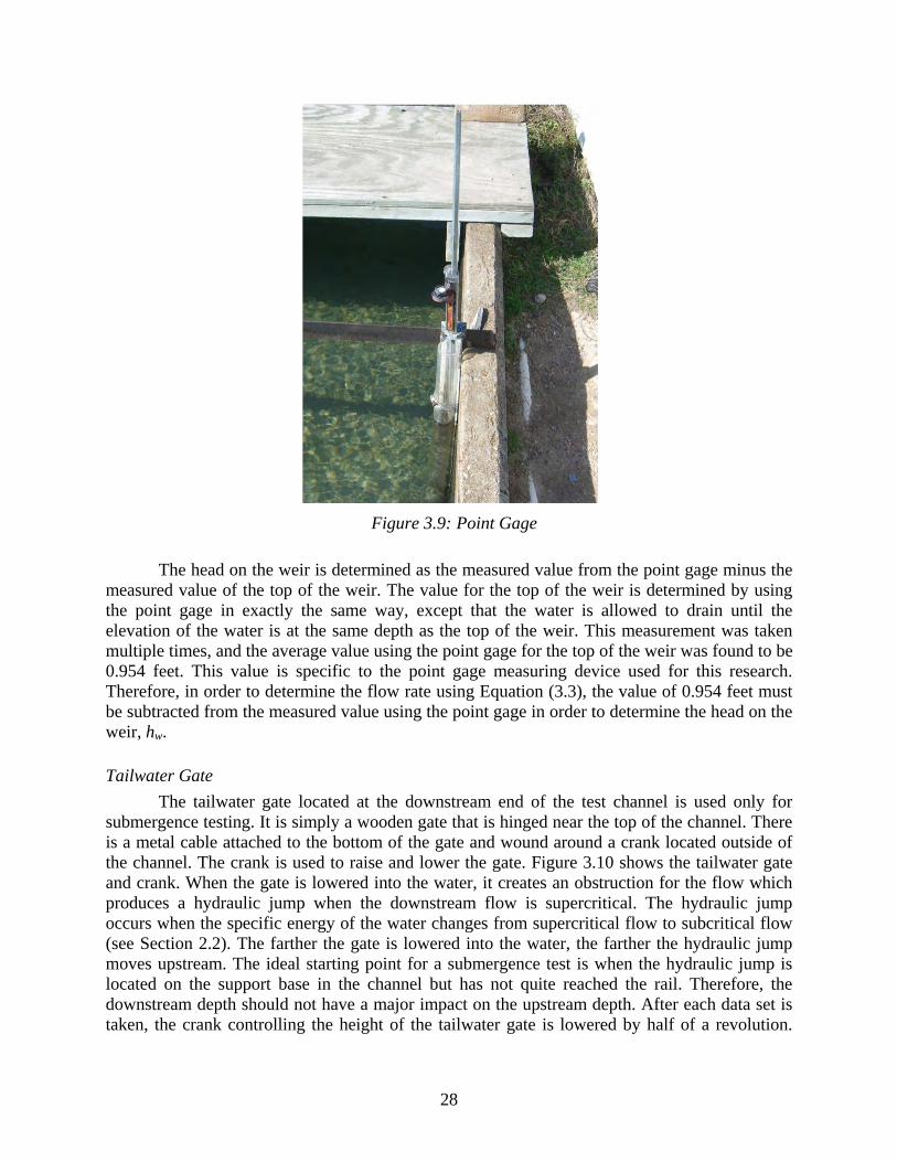
28

Figure 3.9: Point Gage

The head on the weir is determined as the measured value from the point gage minus the measured value of the top of the weir. The value for the top of the weir is determined by using the point gage in exactly the same way, except that the water is allowed to drain until the elevation of the water is at the same depth as the top of the weir. This measurement was taken multiple times, and the average value using the point gage for the top of the weir was found to be 0.954 feet. This value is specific to the point gage measuring device used for this research. Therefore, in order to determine the flow rate using Equation (3.3), the value of 0.954 feet must be subtracted from the measured value using the point gage in order to determine the head on the weir, hw.

Tailwater Gate The tailwater gate located at the downstream end of the test channel is used only for submergence testing. It is simply a wooden gate that is hinged near the top of the channel. There is a metal cable attached to the bottom of the gate and wound around a crank located outside of the channel. The crank is used to raise and lower the gate. Figure 3.10 shows the tailwater gate and crank. When the gate is lowered into the water, it creates an obstruction for the flow which produces a hydraulic jump when the downstream flow is supercritical. The hydraulic jump occurs when the specific energy of the water changes from supercritical flow to subcritical flow (see Section 2.2). The farther the gate is lowered into the water, the farther the hydraulic jump moves upstream. The ideal starting point for a submergence test is when the hydraulic jump is located on the support base in the channel but has not quite reached the rail. Therefore, the downstream depth should not have a major impact on the upstream depth. After each data set is taken, the crank controlling the height of the tailwater gate is lowered by half of a revolution.

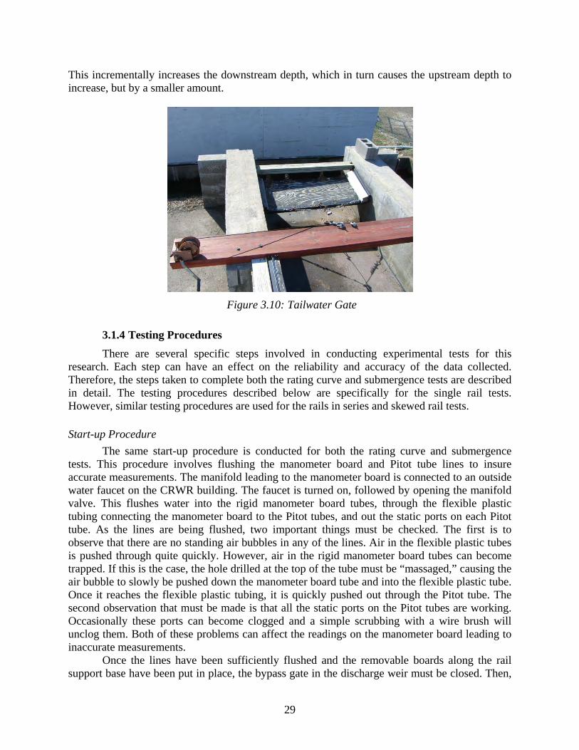
29

This incrementally increases the downstream depth, which in turn causes the upstream depth to increase, but by a smaller amount.

Figure 3.10: Tailwater Gate

3.1.4 Testing Procedures There are several specific steps involved in conducting experimental tests for this research. Each step can have an effect on the reliability and accuracy of the data collected. Therefore, the steps taken to complete both the rating curve and submergence tests are described in detail. The testing procedures described below are specifically for the single rail tests. However, similar testing procedures are used for the rails in series and skewed rail tests.

Start-up Procedure The same start-up procedure is conducted for both the rating curve and submergence tests. This procedure involves flushing the manometer board and Pitot tube lines to insure accurate measurements. The manifold leading to the manometer board is connected to an outside water faucet on the CRWR building. The faucet is turned on, followed by opening the manifold valve. This flushes water into the rigid manometer board tubes, through the flexible plastic tubing connecting the manometer board to the Pitot tubes, and out the static ports on each Pitot tube. As the lines are being flushed, two important things must be checked. The first is to observe that there are no standing air bubbles in any of the lines. Air in the flexible plastic tubes is pushed through quite quickly. However, air in the rigid manometer board tubes can become trapped. If this is the case, the hole drilled at the top of the tube must be “massaged,” causing the air bubble to slowly be pushed down the manometer board tube and into the flexible plastic tube. Once it reaches the flexible plastic tubing, it is quickly pushed out through the Pitot tube. The second observation that must be made is that all the static ports on the Pitot tubes are working. Occasionally these ports can become clogged and a simple scrubbing with a wire brush will unclog them. Both of these problems can affect the readings on the manometer board leading to inaccurate measurements. Once the lines have been sufficiently flushed and the removable boards along the rail support base have been put in place, the bypass gate in the discharge weir must be closed. Then,

30

the pumps are turned on to a desired flow rate. After the Pitot tubes have been submerged in the test channel, the manifold valve can be closed, followed by turning off the water faucet. Submerging the Pitot tubes ensures that no air will re-enter the lines. The pumps are allowed to run a minimum of 45 minutes prior to taking data. This 45 minute initial duration was determined through trial tests before initiation of the research program, and allows for all the return channels to fill with water and reach steady state, thereby resulting in accurate flow rate measurements at the discharge weir.

Rating Curve Testing Procedure When conducting tests for data on the rating curve, the three downstream Pitot tubes are not used. For a given flow rate, three sets of measurements are taken on each of the six upstream Pitot tubes. The arithmetic average of these three sets can be used to calculate the water depth at each of the six Pitot tube locations using Equation (3.2). The arithmetic average of these six locations is used as the upstream water depth. The precision of the manometer board measurements, along the inclined depth, is taken as 0.005 feet measured from the bottom of the meniscus in the tube. In addition to the three depth measurements, three point gage measurements are taken at the discharge weir. The arithmetic average of these three is used to calculate the flow rate using Equation (3.3). The precision of the point gage is 0.001 feet. Slight fluctuations in the depth measurements can occur on the manometer board reading. Therefore, each set of measurements are taken a couple of minutes apart in order to get the average of these fluctuations. Once all three sets of measurements are taken, the flow rate is changed by partially opening or closing the valves from the pumps. The return channels are allowed a minimum of 30 minutes to stabilize to the new flow rate to insure accurate flow rate measurements before the next set of measurements are taken.

Submerged Testing Procedure When conducting submergence test measurements, the downstream tailwater gate is lowered into the water to produce a hydraulic jump. The tailwater gate is lowered to the point where the hydraulic jump is located on the support base but has not quite reached the bridge rail itself. Achieving the desired location of the hydraulic jump is accomplished through a trial and error process of lowering or raising the tailwater gate as appropriate. When the hydraulic jump is located on the support base immediately downstream from the rail, the upstream water depth should not be significantly influenced by the downstream depth. Once the downstream Pitot tubes are submerged by the hydraulic jump, the manifold valve can be closed to insure no air enters the lines. After the return channels have reached steady state, measurements are taken in much the same way as for the rating curve procedure. However, all nine Pitot tubes are used for submergence testing. In addition, six sets of measurements are taken instead of the three sets for rating curve data. The increased number of data sets taken is because there is significant turbulence downstream from the bridge rail at low downstream depths. This turbulence can cause the water depth in the tubes on the manometer board to fluctuate up to a few centimeters. The additional data sets are taken to get the average of these fluctuations for the downstream depth. After each of the six data sets are taken for depth and flow rate at the point gage, the crank controlling the tailwater gate is lower by half of a revolution. This change in the tailwater gate has proven to be sufficient in incrementally increasing the downstream depth.

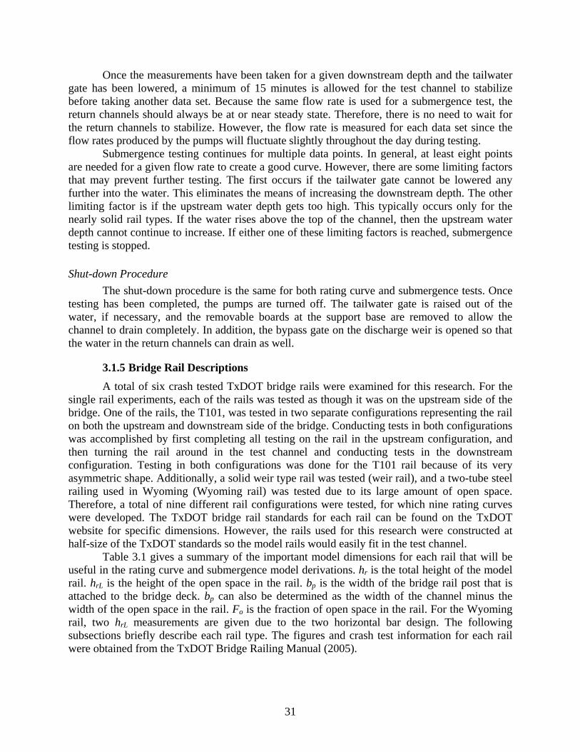
31

Once the measurements have been taken for a given downstream depth and the tailwater gate has been lowered, a minimum of 15 minutes is allowed for the test channel to stabilize before taking another data set. Because the same flow rate is used for a submergence test, the return channels should always be at or near steady state. Therefore, there is no need to wait for the return channels to stabilize. However, the flow rate is measured for each data set since the flow rates produced by the pumps will fluctuate slightly throughout the day during testing. Submergence testing continues for multiple data points. In general, at least eight points are needed for a given flow rate to create a good curve. However, there are some limiting factors that may prevent further testing. The first occurs if the tailwater gate cannot be lowered any further into the water. This eliminates the means of increasing the downstream depth. The other limiting factor is if the upstream water depth gets too high. This typically occurs only for the nearly solid rail types. If the water rises above the top of the channel, then the upstream water depth cannot continue to increase. If either one of these limiting factors is reached, submergence testing is stopped.

Shut-down Procedure The shut-down procedure is the same for both rating curve and submergence tests. Once testing has been completed, the pumps are turned off. The tailwater gate is raised out of the water, if necessary, and the removable boards at the support base are removed to allow the channel to drain completely. In addition, the bypass gate on the discharge weir is opened so that the water in the return channels can drain as well.

3.1.5 Bridge Rail Descriptions A total of six crash tested TxDOT bridge rails were examined for this research. For the single rail experiments, each of the rails was tested as though it was on the upstream side of the bridge. One of the rails, the T101, was tested in two separate configurations representing the rail on both the upstream and downstream side of the bridge. Conducting tests in both configurations was accomplished by first completing all testing on the rail in the upstream configuration, and then turning the rail around in the test channel and conducting tests in the downstream configuration. Testing in both configurations was done for the T101 rail because of its very asymmetric shape. Additionally, a solid weir type rail was tested (weir rail), and a two-tube steel railing used in Wyoming (Wyoming rail) was tested due to its large amount of open space. Therefore, a total of nine different rail configurations were tested, for which nine rating curves were developed. The TxDOT bridge rail standards for each rail can be found on the TxDOT website for specific dimensions. However, the rails used for this research were constructed at half-size of the TxDOT standards so the model rails would easily fit in the test channel. Table 3.1 gives a summary of the important model dimensions for each rail that will be useful in the rating curve and submergence model derivations. hr is the total height of the model rail. hrL is the height of the open space in the rail. bp is the width of the bridge rail post that is attached to the bridge deck. bp can also be determined as the width of the channel minus the width of the open space in the rail. Fo is the fraction of open space in the rail. For the Wyoming rail, two hrL measurements are given due to the two horizontal bar design. The following subsections briefly describe each rail type. The figures and crash test information for each rail were obtained from the TxDOT Bridge Railing Manual (2005).

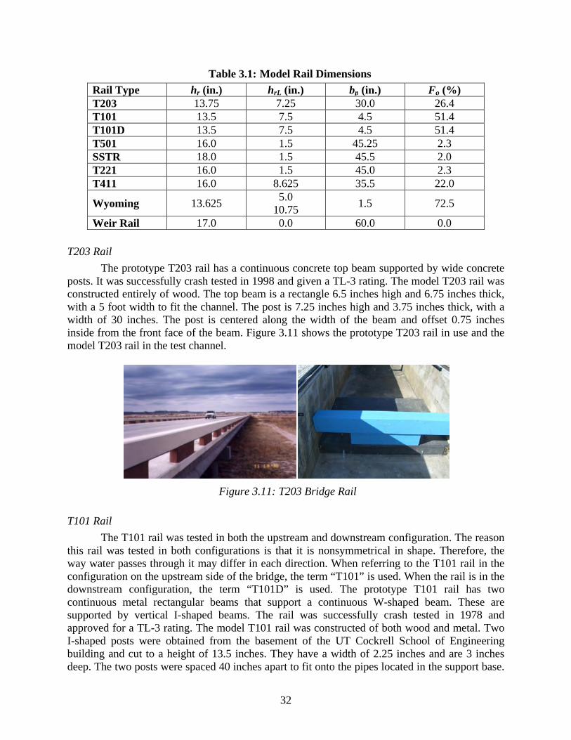
32

Table 3.1: Model Rail Dimensions Rail Type hr (in.) hrL (in.) bp (in.) Fo (%) T203 13.75 7.25 30.0 26.4 T101 13.5 7.5 4.5 51.4 T101D 13.5 7.5 4.5 51.4 T501 16.0 1.5 45.25 2.3 SSTR 18.0 1.5 45.5 2.0 T221 16.0 1.5 45.0 2.3 T411 16.0 8.625 35.5 22.0

Wyoming 13.625 5.0 10.75 1.5 72.5

Weir Rail 17.0 0.0 60.0 0.0

T203 Rail The prototype T203 rail has a continuous concrete top beam supported by wide concrete posts. It was successfully crash tested in 1998 and given a TL-3 rating. The model T203 rail was constructed entirely of wood. The top beam is a rectangle 6.5 inches high and 6.75 inches thick, with a 5 foot width to fit the channel. The post is 7.25 inches high and 3.75 inches thick, with a width of 30 inches. The post is centered along the width of the beam and offset 0.75 inches inside from the front face of the beam. Figure 3.11 shows the prototype T203 rail in use and the model T203 rail in the test channel.

Figure 3.11: T203 Bridge Rail

T101 Rail The T101 rail was tested in both the upstream and downstream configuration. The reason this rail was tested in both configurations is that it is nonsymmetrical in shape. Therefore, the way water passes through it may differ in each direction. When referring to the T101 rail in the configuration on the upstream side of the bridge, the term “T101” is used. When the rail is in the downstream configuration, the term “T101D” is used. The prototype T101 rail has two continuous metal rectangular beams that support a continuous W-shaped beam. These are supported by vertical I-shaped beams. The rail was successfully crash tested in 1978 and approved for a TL-3 rating. The model T101 rail was constructed of both wood and metal. Two I-shaped posts were obtained from the basement of the UT Cockrell School of Engineering building and cut to a height of 13.5 inches. They have a width of 2.25 inches and are 3 inches deep. The two posts were spaced 40 inches apart to fit onto the pipes located in the support base.

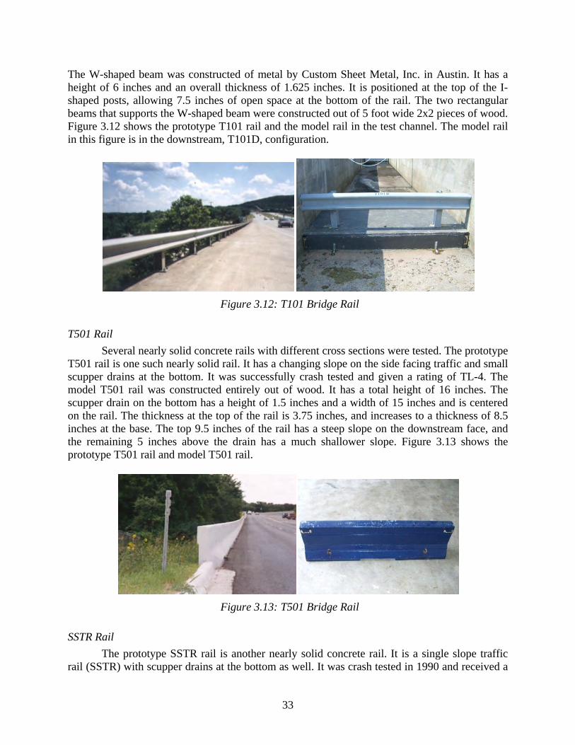
33

The W-shaped beam was constructed of metal by Custom Sheet Metal, Inc. in Austin. It has a height of 6 inches and an overall thickness of 1.625 inches. It is positioned at the top of the I-shaped posts, allowing 7.5 inches of open space at the bottom of the rail. The two rectangular beams that supports the W-shaped beam were constructed out of 5 foot wide 2x2 pieces of wood. Figure 3.12 shows the prototype T101 rail and the model rail in the test channel. The model rail in this figure is in the downstream, T101D, configuration.


T501 Rail Several nearly solid concrete rails with different cross sections were tested. The prototype T501 rail is one such nearly solid rail. It has a changing slope on the side facing traffic and small scupper drains at the bottom. It was successfully crash tested and given a rating of TL-4. The model T501 rail was constructed entirely out of wood. It has a total height of 16 inches. The scupper drain on the bottom has a height of 1.5 inches and a width of 15 inches and is centered on the rail. The thickness at the top of the rail is 3.75 inches, and increases to a thickness of 8.5 inches at the base. The top 9.5 inches of the rail has a steep slope on the downstream face, and the remaining 5 inches above the drain has a much shallower slope. Figure 3.13 shows the prototype T501 rail and model T501 rail.


SSTR Rail The prototype SSTR rail is another nearly solid concrete rail. It is a single slope traffic rail (SSTR) with scupper drains at the bottom as well. It was crash tested in 1990 and received a

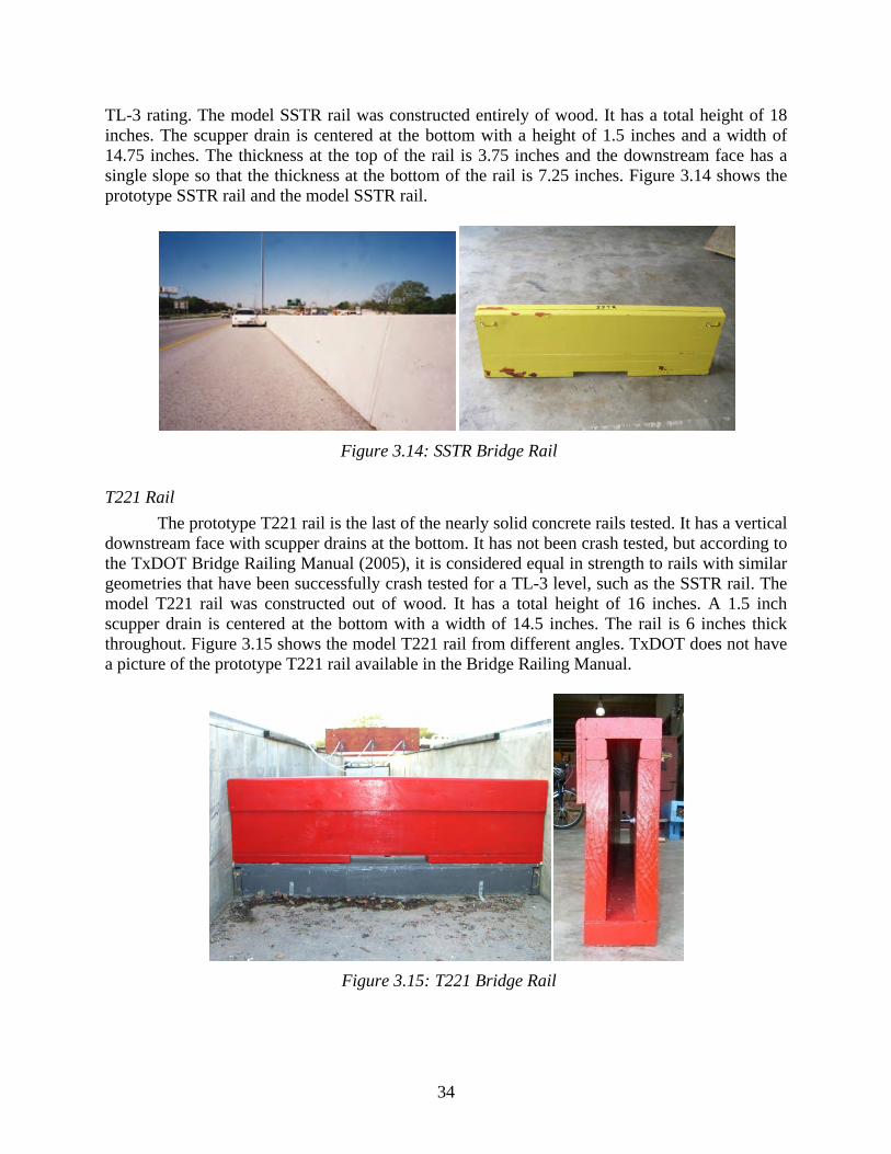
34

TL-3 rating. The model SSTR rail was constructed entirely of wood. It has a total height of 18 inches. The scupper drain is centered at the bottom with a height of 1.5 inches and a width of 14.75 inches. The thickness at the top of the rail is 3.75 inches and the downstream face has a single slope so that the thickness at the bottom of the rail is 7.25 inches. Figure 3.14 shows the prototype SSTR rail and the model SSTR rail.

Figure 3.14: SSTR Bridge Rail

T221 Rail The prototype T221 rail is the last of the nearly solid concrete rails tested. It has a vertical downstream face with scupper drains at the bottom. It has not been crash tested, but according to the TxDOT Bridge Railing Manual (2005), it is considered equal in strength to rails with similar geometries that have been successfully crash tested for a TL-3 level, such as the SSTR rail. The model T221 rail was constructed out of wood. It has a total height of 16 inches. A 1.5 inch scupper drain is centered at the bottom with a width of 14.5 inches. The rail is 6 inches thick throughout. Figure 3.15 shows the model T221 rail from different angles. TxDOT does not have a picture of the prototype T221 rail available in the Bridge Railing Manual.


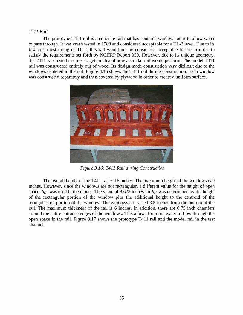
35

T411 Rail The prototype T411 rail is a concrete rail that has centered windows on it to allow water to pass through. It was crash tested in 1989 and considered acceptable for a TL-2 level. Due to its low crash test rating of TL-2, this rail would not be considered acceptable to use in order to satisfy the requirements set forth by NCHRP Report 350. However, due to its unique geometry, the T411 was tested in order to get an idea of how a similar rail would perform. The model T411 rail was constructed entirely out of wood. Its design made construction very difficult due to the windows centered in the rail. Figure 3.16 shows the T411 rail during construction. Each window was constructed separately and then covered by plywood in order to create a uniform surface.

Figure 3.16: T411 Rail during Construction

The overall height of the T411 rail is 16 inches. The maximum height of the windows is 9 inches. However, since the windows are not rectangular, a different value for the height of open space, hrL, was used in the model. The value of 8.625 inches for hrL was determined by the height of the rectangular portion of the window plus the additional height to the centroid of the triangular top portion of the window. The windows are raised 3.5 inches from the bottom of the rail. The maximum thickness of the rail is 6 inches. In addition, there are 0.75 inch chamfers around the entire entrance edges of the windows. This allows for more water to flow through the open space in the rail. Figure 3.17 shows the prototype T411 rail and the model rail in the test channel.

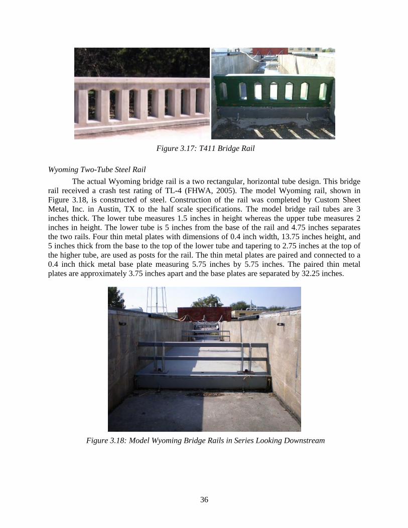
36


Wyoming Two-Tube Steel Rail The actual Wyoming bridge rail is a two rectangular, horizontal tube design. This bridge

rail received a crash test rating of TL-4 (FHWA, 2005). The model Wyoming rail, shown in Figure 3.18, is constructed of steel. Construction of the rail was completed by Custom Sheet Metal, Inc. in Austin, TX to the half scale specifications. The model bridge rail tubes are 3 inches thick. The lower tube measures 1.5 inches in height whereas the upper tube measures 2 inches in height. The lower tube is 5 inches from the base of the rail and 4.75 inches separates the two rails. Four thin metal plates with dimensions of 0.4 inch width, 13.75 inches height, and 5 inches thick from the base to the top of the lower tube and tapering to 2.75 inches at the top of the higher tube, are used as posts for the rail. The thin metal plates are paired and connected to a 0.4 inch thick metal base plate measuring 5.75 inches by 5.75 inches. The paired thin metal plates are approximately 3.75 inches apart and the base plates are separated by 32.25 inches.

Figure 3.18: Model Wyoming Bridge Rails in Series Looking Downstream

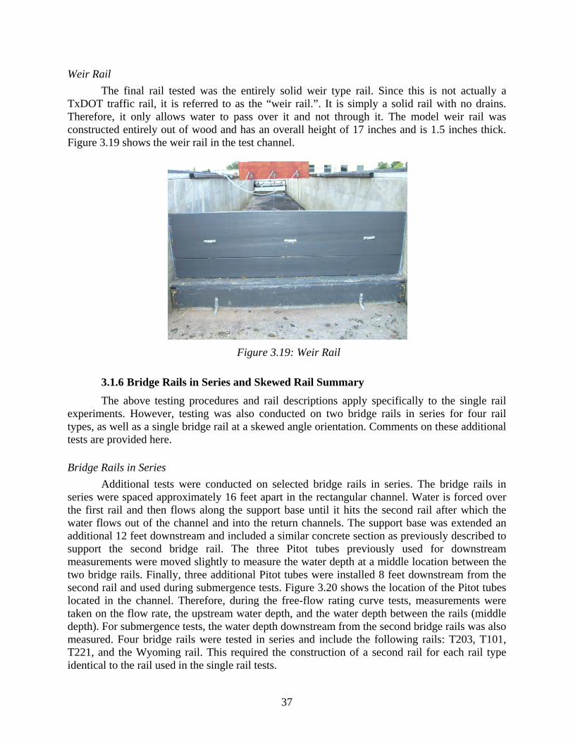
37

Weir Rail The final rail tested was the entirely solid weir type rail. Since this is not actually a TxDOT traffic rail, it is referred to as the “weir rail.”. It is simply a solid rail with no drains. Therefore, it only allows water to pass over it and not through it. The model weir rail was constructed entirely out of wood and has an overall height of 17 inches and is 1.5 inches thick. Figure 3.19 shows the weir rail in the test channel.

Figure 3.19: Weir Rail

3.1.6 Bridge Rails in Series and Skewed Rail Summary The above testing procedures and rail descriptions apply specifically to the single rail experiments. However, testing was also conducted on two bridge rails in series for four rail types, as well as a single bridge rail at a skewed angle orientation. Comments on these additional tests are provided here.

Bridge Rails in Series Additional tests were conducted on selected bridge rails in series. The bridge rails in series were spaced approximately 16 feet apart in the rectangular channel. Water is forced over the first rail and then flows along the support base until it hits the second rail after which the water flows out of the channel and into the return channels. The support base was extended an additional 12 feet downstream and included a similar concrete section as previously described to support the second bridge rail. The three Pitot tubes previously used for downstream measurements were moved slightly to measure the water depth at a middle location between the two bridge rails. Finally, three additional Pitot tubes were installed 8 feet downstream from the second rail and used during submergence tests. Figure 3.20 shows the location of the Pitot tubes located in the channel. Therefore, during the free-flow rating curve tests, measurements were taken on the flow rate, the upstream water depth, and the water depth between the rails (middle depth). For submergence tests, the water depth downstream from the second bridge rails was also measured. Four bridge rails were tested in series and include the following rails: T203, T101, T221, and the Wyoming rail. This required the construction of a second rail for each rail type identical to the rail used in the single rail tests.

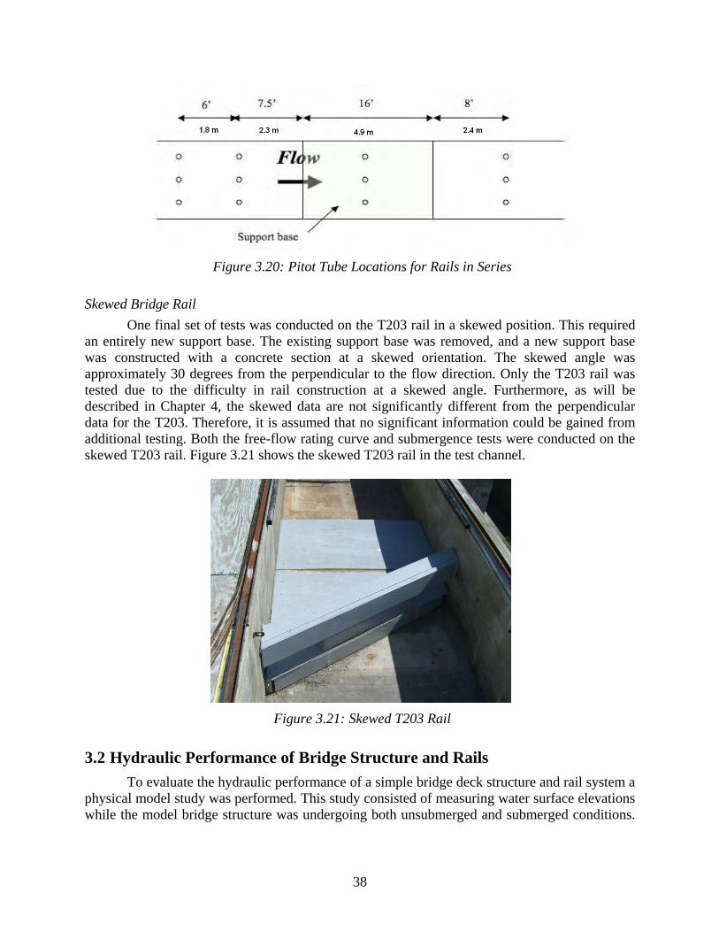
38

Figure 3.20: Pitot Tube Locations for Rails in Series

Skewed Bridge Rail One final set of tests was conducted on the T203 rail in a skewed position. This required an entirely new support base. The existing support base was removed, and a new support base was constructed with a concrete section at a skewed orientation. The skewed angle was approximately 30 degrees from the perpendicular to the flow direction. Only the T203 rail was tested due to the difficulty in rail construction at a skewed angle. Furthermore, as will be described in Chapter 4, the skewed data are not significantly different from the perpendicular data for the T203. Therefore, it is assumed that no significant information could be gained from additional testing. Both the free-flow rating curve and submergence tests were conducted on the skewed T203 rail. Figure 3.21 shows the skewed T203 rail in the test channel.

Figure 3.21: Skewed T203 Rail

3.2 Hydraulic Performance of Bridge Structure and Rails To evaluate the hydraulic performance of a simple bridge deck structure and rail system a

physical model study was performed. This study consisted of measuring water surface elevations while the model bridge structure was undergoing both unsubmerged and submerged conditions.

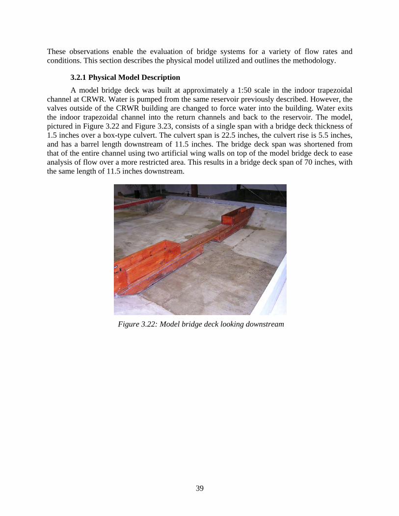
39

These observations enable the evaluation of bridge systems for a variety of flow rates and conditions. This section describes the physical model utilized and outlines the methodology.

3.2.1 Physical Model Description A model bridge deck was built at approximately a 1:50 scale in the indoor trapezoidal

channel at CRWR. Water is pumped from the same reservoir previously described. However, the valves outside of the CRWR building are changed to force water into the building. Water exits the indoor trapezoidal channel into the return channels and back to the reservoir. The model, pictured in Figure 3.22 and Figure 3.23, consists of a single span with a bridge deck thickness of 1.5 inches over a box-type culvert. The culvert span is 22.5 inches, the culvert rise is 5.5 inches, and has a barrel length downstream of 11.5 inches. The bridge deck span was shortened from that of the entire channel using two artificial wing walls on top of the model bridge deck to ease analysis of flow over a more restricted area. This results in a bridge deck span of 70 inches, with the same length of 11.5 inches downstream.

Figure 3.22: Model bridge deck looking downstream

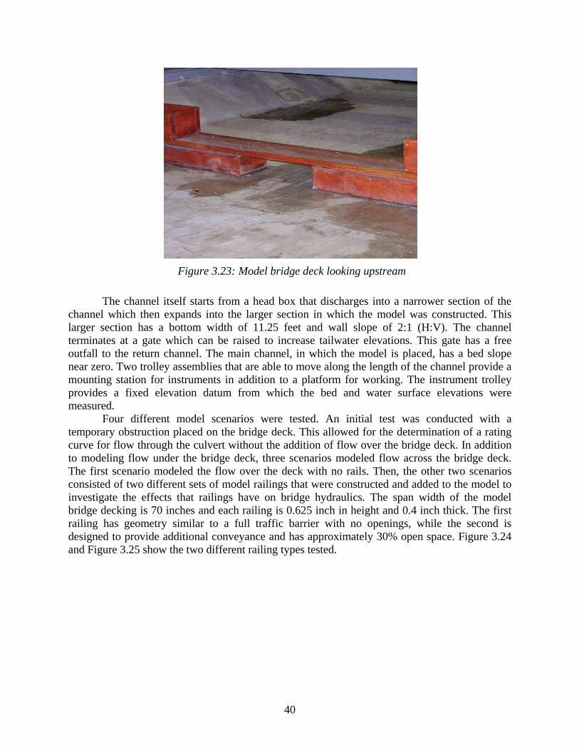
40

Figure 3.23: Model bridge deck looking upstream

The channel itself starts from a head box that discharges into a narrower section of the channel which then expands into the larger section in which the model was constructed. This larger section has a bottom width of 11.25 feet and wall slope of 2:1 (H:V). The channel terminates at a gate which can be raised to increase tailwater elevations. This gate has a free outfall to the return channel. The main channel, in which the model is placed, has a bed slope near zero. Two trolley assemblies that are able to move along the length of the channel provide a mounting station for instruments in addition to a platform for working. The instrument trolley provides a fixed elevation datum from which the bed and water surface elevations were measured.

Four different model scenarios were tested. An initial test was conducted with a temporary obstruction placed on the bridge deck. This allowed for the determination of a rating curve for flow through the culvert without the addition of flow over the bridge deck. In addition to modeling flow under the bridge deck, three scenarios modeled flow across the bridge deck. The first scenario modeled the flow over the deck with no rails. Then, the other two scenarios consisted of two different sets of model railings that were constructed and added to the model to investigate the effects that railings have on bridge hydraulics. The span width of the model bridge decking is 70 inches and each railing is 0.625 inch in height and 0.4 inch thick. The first railing has geometry similar to a full traffic barrier with no openings, while the second is designed to provide additional conveyance and has approximately 30% open space. Figure 3.24 and Figure 3.25 show the two different railing types tested.

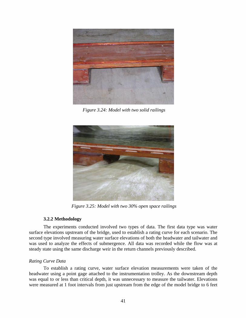
41

Figure 3.24: Model with two solid railings

Figure 3.25: Model with two 30% open space railings

3.2.2 Methodology

The experiments conducted involved two types of data. The first data type was water surface elevations upstream of the bridge, used to establish a rating curve for each scenario. The second type involved measuring water surface elevations of both the headwater and tailwater and was used to analyze the effects of submergence. All data was recorded while the flow was at steady state using the same discharge weir in the return channels previously described.

Rating Curve Data To establish a rating curve, water surface elevation measurements were taken of the

headwater using a point gage attached to the instrumentation trolley. As the downstream depth was equal to or less than critical depth, it was unnecessary to measure the tailwater. Elevations were measured at 1 foot intervals from just upstream from the edge of the model bridge to 6 feet

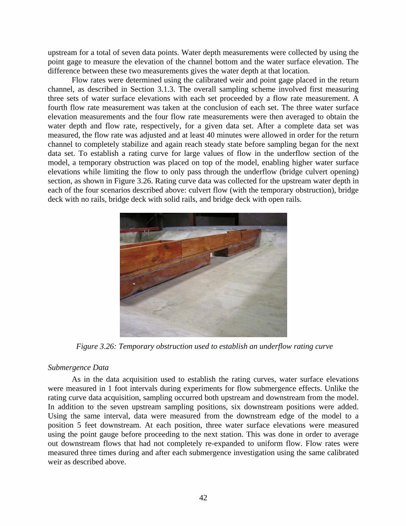
42

upstream for a total of seven data points. Water depth measurements were collected by using the point gage to measure the elevation of the channel bottom and the water surface elevation. The difference between these two measurements gives the water depth at that location.

Flow rates were determined using the calibrated weir and point gage placed in the return channel, as described in Section 3.1.3. The overall sampling scheme involved first measuring three sets of water surface elevations with each set proceeded by a flow rate measurement. A fourth flow rate measurement was taken at the conclusion of each set. The three water surface elevation measurements and the four flow rate measurements were then averaged to obtain the water depth and flow rate, respectively, for a given data set. After a complete data set was measured, the flow rate was adjusted and at least 40 minutes were allowed in order for the return channel to completely stabilize and again reach steady state before sampling began for the next data set. To establish a rating curve for large values of flow in the underflow section of the model, a temporary obstruction was placed on top of the model, enabling higher water surface elevations while limiting the flow to only pass through the underflow (bridge culvert opening) section, as shown in Figure 3.26. Rating curve data was collected for the upstream water depth in each of the four scenarios described above: culvert flow (with the temporary obstruction), bridge deck with no rails, bridge deck with solid rails, and bridge deck with open rails.

Figure 3.26: Temporary obstruction used to establish an underflow rating curve

Submergence Data As in the data acquisition used to establish the rating curves, water surface elevations

were measured in 1 foot intervals during experiments for flow submergence effects. Unlike the rating curve data acquisition, sampling occurred both upstream and downstream from the model. In addition to the seven upstream sampling positions, six downstream positions were added. Using the same interval, data were measured from the downstream edge of the model to a position 5 feet downstream. At each position, three water surface elevations were measured using the point gauge before proceeding to the next station. This was done in order to average out downstream flows that had not completely re-expanded to uniform flow. Flow rates were measured three times during and after each submergence investigation using the same calibrated weir as described above.

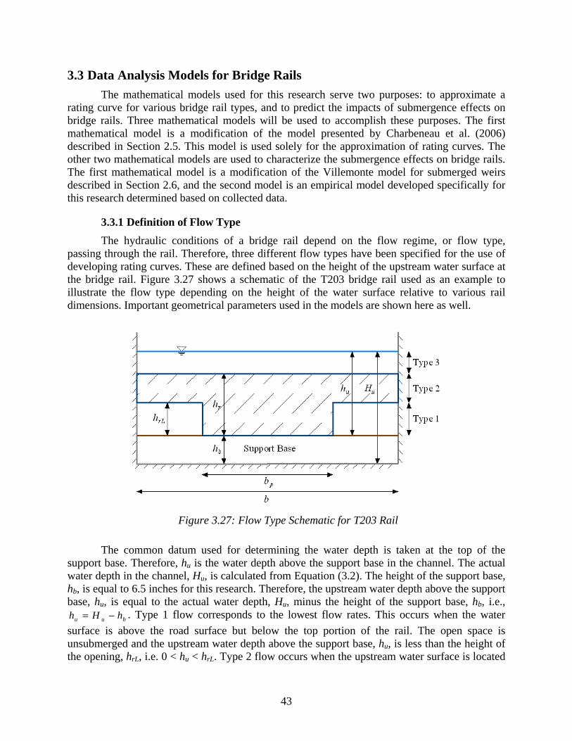
43

3.3 Data Analysis Models for Bridge Rails The mathematical models used for this research serve two purposes: to approximate a rating curve for various bridge rail types, and to predict the impacts of submergence effects on bridge rails. Three mathematical models will be used to accomplish these purposes. The first mathematical model is a modification of the model presented by Charbeneau et al. (2006) described in Section 2.5. This model is used solely for the approximation of rating curves. The other two mathematical models are used to characterize the submergence effects on bridge rails. The first mathematical model is a modification of the Villemonte model for submerged weirs described in Section 2.6, and the second model is an empirical model developed specifically for this research determined based on collected data.

3.3.1 Definition of Flow Type

The hydraulic conditions of a bridge rail depend on the flow regime, or flow type, passing through the rail. Therefore, three different flow types have been specified for the use of developing rating curves. These are defined based on the height of the upstream water surface at the bridge rail. Figure 3.27 shows a schematic of the T203 bridge rail used as an example to illustrate the flow type depending on the height of the water surface relative to various rail dimensions. Important geometrical parameters used in the models are shown here as well.

Figure 3.27: Flow Type Schematic for T203 Rail

The common datum used for determining the water depth is taken at the top of the support base. Therefore, hu is the water depth above the support base in the channel. The actual water depth in the channel, Hu, is calculated from Equation (3.2). The height of the support base, hb, is equal to 6.5 inches for this research. Therefore, the upstream water depth above the support base, hu, is equal to the actual water depth, Hu, minus the height of the support base, hb, i.e.,

buu hHh −= . Type 1 flow corresponds to the lowest flow rates. This occurs when the water surface is above the road surface but below the top portion of the rail. The open space is unsubmerged and the upstream water depth above the support base, hu, is less than the height of the opening, hrL, i.e. 0 < hu < hrL. Type 2 flow occurs when the upstream water surface is located

44

above the base of the rail. The open space is now submerged, and the upstream water depth is greater than the height of the open space but less than the total height of the rail, i.e. hrL < hu < hr. Finally, Type 3 flow occurs when the upstream water depth is greater than the total height of the rail. In this case, the open space is still submerged, but now water is also flowing over the top of the rail similar to weir type flow, i.e. hr < hu. Figure 3.27 also defines several other variables. The channel width, b, is equal to five feet for this research. bp is the width of the bridge rail post, or the channel width minus the width of the open space.

3.3.2 Rating Curve Model Derivation The original rating curve model, presented by Charbeneau et al. (2006) and described in Section 2.5, uses two parameters for flow through a highway culvert. The first parameter, Cb, is used during unsubmerged flow through the culvert and can be thought of as a contraction coefficient for the entrance edge conditions along the width of the culvert in the horizontal dimension. The second parameter, Cc, along with Cb, is used during submerged flow through the culvert. Cc also represents a contraction coefficient but applies to the vertical dimension of the culvert. Both parameters are also used to account for minor losses that have been assumed negligible in the model derivation. For the bridge rail rating curve model, a third parameter, Cd, is introduced that acts in the same way as the discharge coefficient in the weir equation (see Equation (2.10)). The same symbol is used here since flow over the rail will be modeled using the weir equation. Therefore, we will have three parameters that will be used to describe the three types of flow that can occur through a bridge rail. For Type 1 flow, only Cb is used; for Type 2 flow, Cb and Cc are used; and for Type 3 flow, Cb, Cc, and Cd are all used.

Type 1 Flow For Type 1 flow, following the Charbeneau et al. (2006) model, the assumption is made that critical depth occurs at or near the location of the bridge rail. This assumption is reasonable because the bridge rail will force the flow through critical depth since it acts as a controlling constriction, or choke, in the channel. A choke is considered a constriction that is severe enough to influence the upstream flow conditions (Henderson, 1966). In the case of a bridge rail, the upstream flow becomes subcritical as a result of passing through the rail. Therefore, at or near the choke section, the flow will pass through a critical condition, followed by a supercritical condition downstream (assuming there are no additional downstream constrictions). Since critical flow occurs at or near the bridge rail, we can use the definition of critical depth as derived in Equation (2.8) and repeated here, with bb hz = . This is the starting point for developing the mathematical rating curve model.

( ) ubuc ehEh32

32 =−= (3.4)

In Equation (3.4), eu = Eu – hb is the base-scaled specific energy, which is the upstream specific energy measured with the bridge decking as a datum. The flow rate can be calculated using the continuity equation, along with the critical velocity determined from the definition of the Froude number. Since it is assumed that critical depth occurs for Type 1 flow, the Froude number (see Equation (2.25)) will be equal to a value of one, so that cc ghv = . Equation (3.5) derives the flow rate at the location of critical depth based on the model assumptions described by Charbeneau et al.

45

ccpbc ghhbbCAvQ )( −== (3.5) A is equal to the cross-sectional area of flow. Based on the model assumptions, the area of flow is equal to the height of water, hc, times the width of the open space in the rail, pbb − , times the contraction coefficient in the horizontal direction, Cb. One may define the fraction of open space, Fo, for a rail as the amount of open area, Ao, in the rail divided by the total area of the rail, Ar. The fraction of open space gives a measure of the relative amount of area available for water to pass through the rail and is considered an important design parameter. Fo is therefore:

r

rLp

r

oo bh

hbbAAF

)( −== (3.6)

In order to easily compare rating curves between different bridge rails, it is helpful to look at the flow rate as a dimensionless parameter. Therefore, combining Equations (3.4), (3.5), and (3.6) and applying algebra to non-dimensionalize, one finds:

5.1

3 32

⎟⎟⎠

⎞⎜⎜⎝

⎛⎟⎟⎠

⎞⎜⎜⎝

⎛=≡

r

u

rL

rob

rrr he

hhFC

gh

qghA

Q (3.7)

The flow rate, Q, in Equation (3.7) is divided by the width of the channel, b, which is included in the Ar term. As defined in Equation (2.3), the flow rate per unit width results a unit flow rate, q. The use of a unit flow rate allows the non-dimensional flow rate equation to be applicable to any rail on a bridge of any width, and this formulation is used below.

Type 2 Flow Type 2 flow is modeled as orifice or sluice type flow according to the model proposed by Charbeneau et al. (2006). The derivation follows similar steps as for Type 1 flow. Type 2 flow is derived by applying the equation for specific energy (see Equation (2.2)), and assuming that the specific energy at a location upstream from the model rail is the same as the specific energy at the model rail. In addition, it is assumed that the upstream flow regime will be subcritical due to the obstruction created by the bridge rail. The upstream velocity head is small but not necessarily negligible. The energy equation gives

g

vhCh

gv

hhE mrLcb

mmbu 22

22

++=++= (3.8)

In Equation (3.8) hm is the water depth located at the model rail and vm is the velocity at the model rail. According to the Charbeneau et al. model, hm is equal to Cc times hrL. Solving for vm gives the following:

46

)(2 rLcbum hChEgv −−= (3.9) Again using the continuity equation, one can determine the flow rate: mrLcpbm vhCbbCAvQ )( −== (3.10) After several steps of algebra, combining Equations (3.9) and (3.10), one can obtain the non-dimensional equation for flow rate.

⎟⎟⎠

⎞⎜⎜⎝

⎛−=

r

rLc

r

uocb

rhhC

heFCC

gh

q 23

(3.11)

In order to determine where the transition between Type 1 flow and Type 2 flow occurs, one can set Equation (3.7) equal to Equation (3.11). This equality results in a cubic equation in terms of eu. The three roots are equal to -3 and 3/2 (the latter is a double root). Since the negative root has no physical meaning, the only applicable value is 3/2. Therefore, the transition between Type 1 flow and Type 2 flow occurs at a water depth defined by Equation (3.12), which is normalized to the height of the rail.

r

rLc

r

u

hhC

he

23= (3.12)

As mentioned in Chapter 2, at this point the derivative of the curves specified by Equations (3.7) and (3.11) are equal so that the curves become tangent, creating a smooth transition point.

Type 3 Flow Type 3 flow is modeled as a combination of orifice flow and weir flow. In order to model Type 3 flow, the assumption is made that the superposition of orifice and weir flow is applicable. This assumption fits well with the experimental data, as shown in Chapter 4. It also follows the same principles of superposition used in deriving the Villemonte submergence model described in Chapter 2. Using the equation for a broad-crested weir from Chapter 2 to obtain the discharge and assuming Cv = 1.0 leads to the following.

5.1)(32

32

rud hegCq −= (3.13)

where hw in Equation (2.11) is replaced with (eu – hr). The use of a broad-crested weir, as opposed to a sharp-crested weir, is used here because of the varying thicknesses of the different rail types. Also, when determining the non-dimensional form of the broad-crested weir equation, the result has a simpler form than that of the sharp-crested weir equation. Converting Equation (3.13) into a non-dimensional form and adding the result to the equation for Type 2 flow (see Equation (3.11)) results in the following.

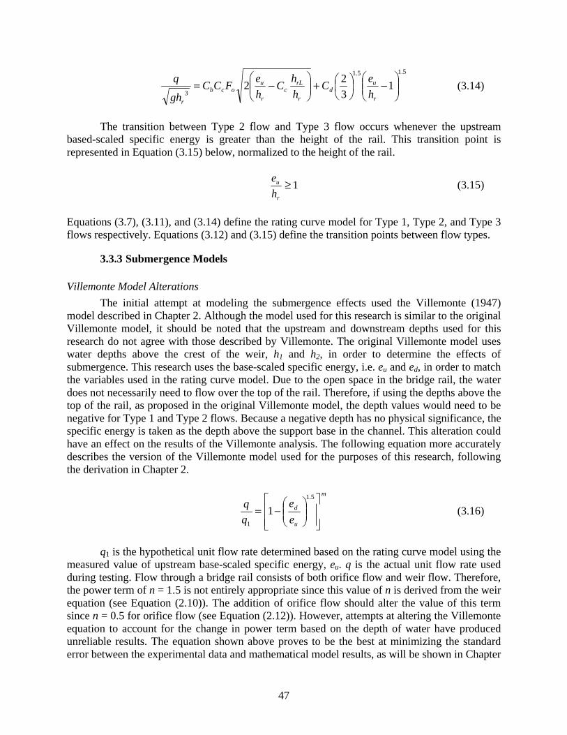
47

5.15.1

31

322 ⎟⎟

⎠

⎞⎜⎜⎝

⎛−⎟

⎠⎞

⎜⎝⎛+⎟⎟

⎠

⎞⎜⎜⎝

⎛−=

r

ud

r

rLc

r

uocb

rheC

hhC

heFCC

gh

q (3.14)

The transition between Type 2 flow and Type 3 flow occurs whenever the upstream based-scaled specific energy is greater than the height of the rail. This transition point is represented in Equation (3.15) below, normalized to the height of the rail.

1≥r

u

he (3.15)

Equations (3.7), (3.11), and (3.14) define the rating curve model for Type 1, Type 2, and Type 3 flows respectively. Equations (3.12) and (3.15) define the transition points between flow types.

3.3.3 Submergence Models

Villemonte Model Alterations The initial attempt at modeling the submergence effects used the Villemonte (1947) model described in Chapter 2. Although the model used for this research is similar to the original Villemonte model, it should be noted that the upstream and downstream depths used for this research do not agree with those described by Villemonte. The original Villemonte model uses water depths above the crest of the weir, h1 and h2, in order to determine the effects of submergence. This research uses the base-scaled specific energy, i.e. eu and ed, in order to match the variables used in the rating curve model. Due to the open space in the bridge rail, the water does not necessarily need to flow over the top of the rail. Therefore, if using the depths above the top of the rail, as proposed in the original Villemonte model, the depth values would need to be negative for Type 1 and Type 2 flows. Because a negative depth has no physical significance, the specific energy is taken as the depth above the support base in the channel. This alteration could have an effect on the results of the Villemonte analysis. The following equation more accurately describes the version of the Villemonte model used for the purposes of this research, following the derivation in Chapter 2.

m

u

d

ee

qq

⎥⎥⎦

⎤

⎢⎢⎣

⎡⎟⎟⎠

⎞⎜⎜⎝

⎛−=

5.1

1

1 (3.16)

q1 is the hypothetical unit flow rate determined based on the rating curve model using the measured value of upstream base-scaled specific energy, eu. q is the actual unit flow rate used during testing. Flow through a bridge rail consists of both orifice flow and weir flow. Therefore, the power term of n = 1.5 is not entirely appropriate since this value of n is derived from the weir equation (see Equation (2.10)). The addition of orifice flow should alter the value of this term since n = 0.5 for orifice flow (see Equation (2.12)). However, attempts at altering the Villemonte equation to account for the change in power term based on the depth of water have produced unreliable results. The equation shown above proves to be the best at minimizing the standard error between the experimental data and mathematical model results, as will be shown in Chapter

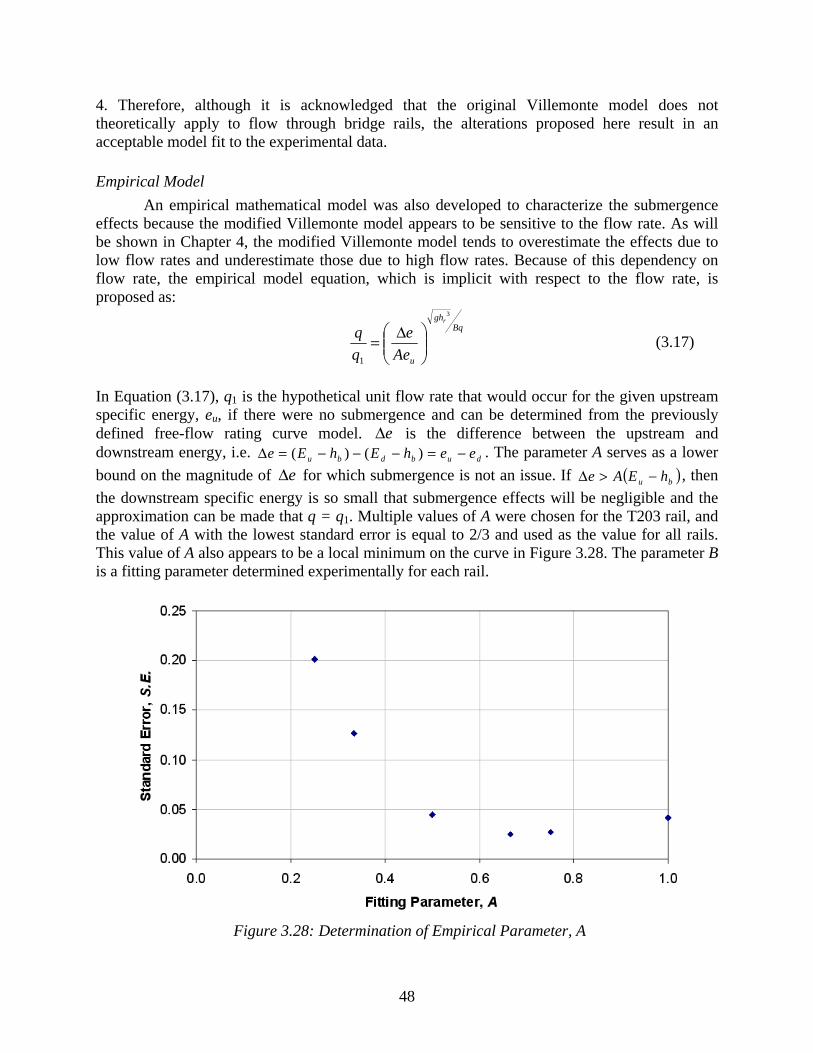
48

4. Therefore, although it is acknowledged that the original Villemonte model does not theoretically apply to flow through bridge rails, the alterations proposed here result in an acceptable model fit to the experimental data.

Empirical Model An empirical mathematical model was also developed to characterize the submergence effects because the modified Villemonte model appears to be sensitive to the flow rate. As will be shown in Chapter 4, the modified Villemonte model tends to overestimate the effects due to low flow rates and underestimate those due to high flow rates. Because of this dependency on flow rate, the empirical model equation, which is implicit with respect to the flow rate, is proposed as:

Bq

gh

u

r

Aee

qq

3

1⎟⎟⎠

⎞⎜⎜⎝

⎛ Δ= (3.17)

In Equation (3.17), q1 is the hypothetical unit flow rate that would occur for the given upstream specific energy, eu, if there were no submergence and can be determined from the previously defined free-flow rating curve model. eΔ is the difference between the upstream and downstream energy, i.e. dubdbu eehEhEe −=−−−=Δ )()( . The parameter A serves as a lower bound on the magnitude of eΔ for which submergence is not an issue. If ( )bu hEAe −>Δ , then the downstream specific energy is so small that submergence effects will be negligible and the approximation can be made that q = q1. Multiple values of A were chosen for the T203 rail, and the value of A with the lowest standard error is equal to 2/3 and used as the value for all rails. This value of A also appears to be a local minimum on the curve in Figure 3.28. The parameter B is a fitting parameter determined experimentally for each rail.

Figure 3.28: Determination of Empirical Parameter, A

49

This model is simple and easy to use for testing purposes in determining the value of the parameter B. However, it is not as easy to use for predicting submergence conditions where the flow rate is unknown. Because the empirical model is implicit with respect to flow rate, Equation (3.17) must be solved iteratively in order to determine the unknown flow rate. An example in Chapter 4 of this report describes how to solve this iterative problem.

50

51

Chapter 4. Experiment Results and Analysis

The main purpose of this research is to determine the hydraulic performance of bridge rails and to provide TxDOT with rail rating curves and analysis of the submergence effects used to describe hydraulic performance. A comparison of the rating curves for each rail to the others will show which rail has the best relative hydraulic efficiency. Analysis of the submergence effects will show how increases in downstream water depth will increase the upstream depth greater than the values predicted with the rating curves. Additionally, it is important to develop procedures to include bridge rail hydraulic data in floodplain analysis models such as HEC-RAS. These issues are addressed in this chapter and the following.

4.1 Rating Curve Results

4.1.1 Observed Data and Analysis of the T203 Rail

The rating curves for a bridge rail describe the upstream water depth as a function of the channel flow rate. Therefore, these were the only two measurements needed to develop the curves. As previously mentioned, the upstream depth was taken three separate times at six different locations, and the arithmetic average of these 18 points was used as the upstream water depth. To calculate the flow rate, three separate measurements were taken to determine the head on the weir. The arithmetic average of these three measurements was used to calculate the flow rate using the weir equation (see Equation (3.3)). During the data collection process, the nappe flowing over the rail during Type 3 flows periodically lost aeration. During certain flow rates, aeration of the nappe becomes a concern. At low flow rates during Type 3 flow, it appeared that the nappe was always aerated. Conversely, at very high flow rates it was obvious that the nappe was no longer aerated. This was observed by the fact that there was no air under the nappe, and the nappe was attached to the downstream face of the bridge rail. Although this is not an ideal situation, there is no way to aerate the nappe on actual bridge rails during a flood event. Therefore, no effort was made to do so during testing. On the other hand, the lack of nappe aeration on the model rail could coincide with the loss of nappe aeration on the prototype rail. If the loss of aeration on the model rail occurs under the same scale conditions as the loss of aeration on the prototype rail, then the experimental data obtained in this research should match the actual rating curve of the prototype rail. However, whether the loss of aeration on both the model and prototype rails occurs under the same conditions is not known. The aeration under the nappe is a concern during the transition flow rates between complete aeration and no aeration. In these intermediate flow rates, the nappe would slowly lose aeration followed by spontaneously reaerating itself. This would cause the water level in the manometer board to slowly fall as air was removed from under the nappe and then quickly rise when reaeration took place. This can easily be seen in the rating curve data for the T101D rail shown in Figure 4.6 below. At the upper end of the rating curve there is significant spread in the data as a result of the uncontrolled aeration of the nappe. Unfortunately, for the T101D rail, this additional uncertainty occurred at the maximum flow rates obtainable. Therefore, the curvature of the Type 3 flow obtained by the rating curve model (described in the next section) is questionable. For most other rails, the aeration problems arose during intermediate flow rates. The loss of aeration at intermediate flow rates is less of a concern because the lower flow rates and higher flow rates are represented quite well and tend to reduce

52

the problems that arise due to nappe aeration. In Figure 4.1, three different stages of nappe aeration can be seen for the T501 rail during testing. Figure 4.1(a) shows the nappe when it is completely aerated. Figure 4.1(b) shows partial aeration of the nappe. Here, portions of the nappe have begun to attach to the downstream face of the rail. Figure 4.1(c) shows the nappe with no aeration, and it is completely attached to the rail.

Figure 4.1: Nappe Aeration Stages a) Complete Nappe Aeration, b) Partial Nappe Aeration, c) No Nappe Aeration

The T203 bridge rail shown in Figure 3.11 and 3.27 is considered to outline the model fitting procedure. The primary data measured includes the upstream water depth Hu and the discharge Q (or unit discharge, q = Q/b, where b is the channel width). The measured data for the T203 rail is shown in Figure 4.2. The depth and discharge values are used to calculate the upstream specific energy Eu and base-scaled specific energy eu as follows.

The discharge and specific energy values are used with model equations (3.7), (3.11), and (3.14), along with transition equations (3.12) and (3.15) to estimate the model parameters Cb, Cc, and Cd

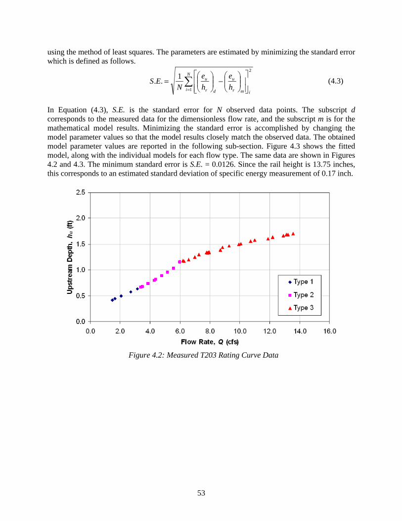
53

using the method of least squares. The parameters are estimated by minimizing the standard error which is defined as follows.

2

1

1..i

N

i mr

u

dr

u

he

he

NES ∑

= ⎥⎥⎦

⎤

⎢⎢⎣

⎡⎟⎟⎠

⎞⎜⎜⎝

⎛−⎟⎟

⎠

⎞⎜⎜⎝

⎛= (4.3)

In Equation (4.3), S.E. is the standard error for N observed data points. The subscript d corresponds to the measured data for the dimensionless flow rate, and the subscript m is for the mathematical model results. Minimizing the standard error is accomplished by changing the model parameter values so that the model results closely match the observed data. The obtained model parameter values are reported in the following sub-section. Figure 4.3 shows the fitted model, along with the individual models for each flow type. The same data are shown in Figures 4.2 and 4.3. The minimum standard error is S.E. = 0.0126. Since the rail height is 13.75 inches, this corresponds to an estimated standard deviation of specific energy measurement of 0.17 inch.

Figure 4.2: Measured T203 Rating Curve Data

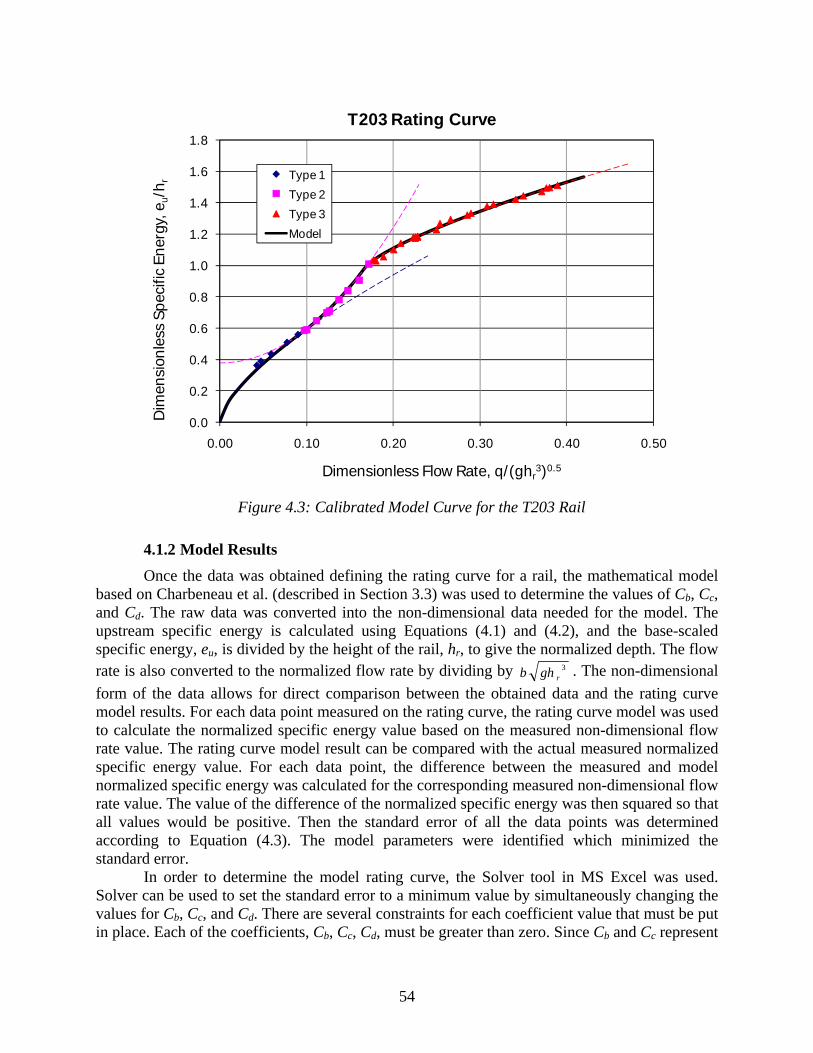
54

Figure 4.3: Calibrated Model Curve for the T203 Rail

4.1.2 Model Results

Once the data was obtained defining the rating curve for a rail, the mathematical model based on Charbeneau et al. (described in Section 3.3) was used to determine the values of Cb, Cc, and Cd. The raw data was converted into the non-dimensional data needed for the model. The upstream specific energy is calculated using Equations (4.1) and (4.2), and the base-scaled specific energy, eu, is divided by the height of the rail, hr, to give the normalized depth. The flow rate is also converted to the normalized flow rate by dividing by 3

rghb . The non-dimensional form of the data allows for direct comparison between the obtained data and the rating curve model results. For each data point measured on the rating curve, the rating curve model was used to calculate the normalized specific energy value based on the measured non-dimensional flow rate value. The rating curve model result can be compared with the actual measured normalized specific energy value. For each data point, the difference between the measured and model normalized specific energy was calculated for the corresponding measured non-dimensional flow rate value. The value of the difference of the normalized specific energy was then squared so that all values would be positive. Then the standard error of all the data points was determined according to Equation (4.3). The model parameters were identified which minimized the standard error. In order to determine the model rating curve, the Solver tool in MS Excel was used. Solver can be used to set the standard error to a minimum value by simultaneously changing the values for Cb, Cc, and Cd. There are several constraints for each coefficient value that must be put in place. Each of the coefficients, Cb, Cc, Cd, must be greater than zero. Since Cb and Cc represent

0.0

0.2

0.4

0.6

0.8

1.0

1.2

1.4

1.6

1.8

0.00 0.10 0.20 0.30 0.40 0.50

Dim

ensi

onle

ss S

peci

fic E

nerg

y, e

u/h r

Dimensionless Flow Rate, q/(ghr3)0.5

T203 Rating Curve

Type 1

Type 2

Type 3

Model

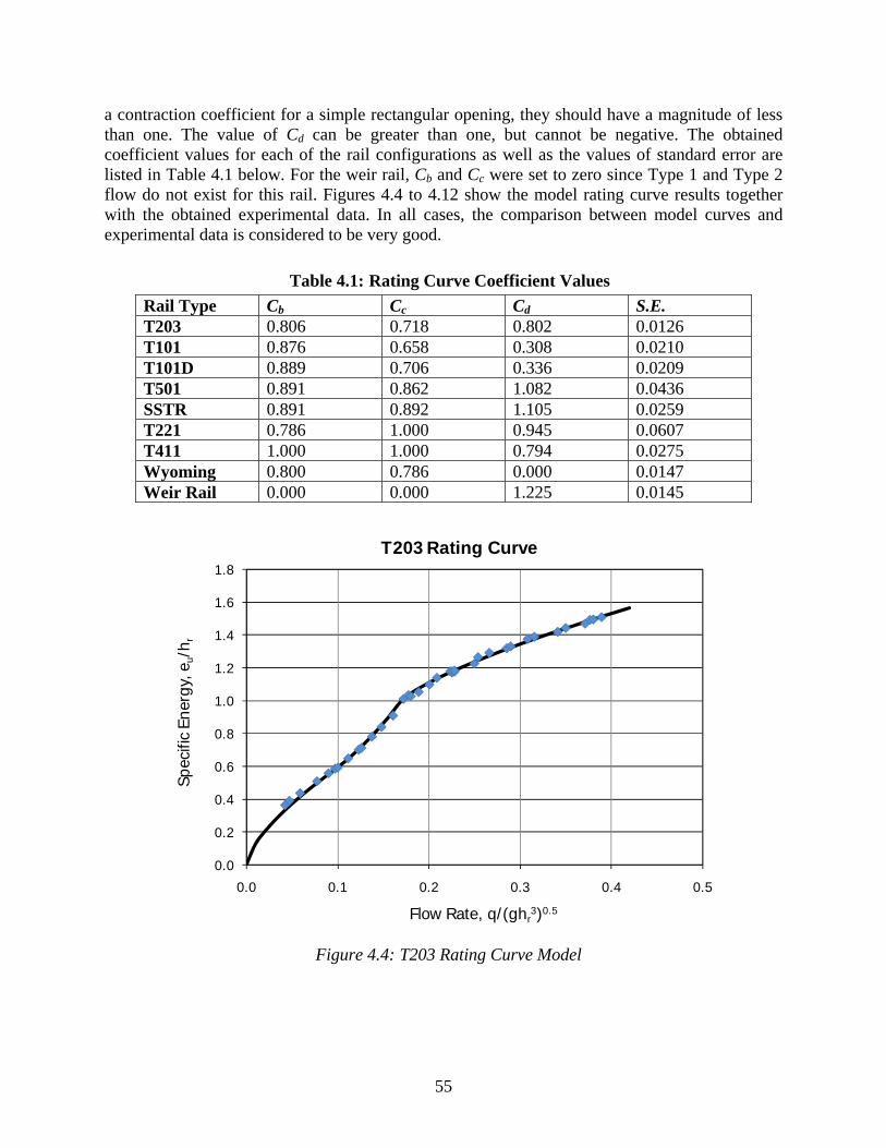
55

a contraction coefficient for a simple rectangular opening, they should have a magnitude of less than one. The value of Cd can be greater than one, but cannot be negative. The obtained coefficient values for each of the rail configurations as well as the values of standard error are listed in Table 4.1 below. For the weir rail, Cb and Cc were set to zero since Type 1 and Type 2 flow do not exist for this rail. Figures 4.4 to 4.12 show the model rating curve results together with the obtained experimental data. In all cases, the comparison between model curves and experimental data is considered to be very good.

Table 4.1: Rating Curve Coefficient Values Rail Type Cb Cc Cd S.E. T203 0.806 0.718 0.802 0.0126 T101 0.876 0.658 0.308 0.0210 T101D 0.889 0.706 0.336 0.0209 T501 0.891 0.862 1.082 0.0436 SSTR 0.891 0.892 1.105 0.0259 T221 0.786 1.000 0.945 0.0607 T411 1.000 1.000 0.794 0.0275 Wyoming 0.800 0.786 0.000 0.0147 Weir Rail 0.000 0.000 1.225 0.0145

Figure 4.4: T203 Rating Curve Model

0.0

0.2

0.4

0.6

0.8

1.0

1.2

1.4

1.6

1.8

0.0 0.1 0.2 0.3 0.4 0.5

Spec

ific

Ener

gy, e

u/h r

Flow Rate, q/(ghr3)0.5

T203 Rating Curve

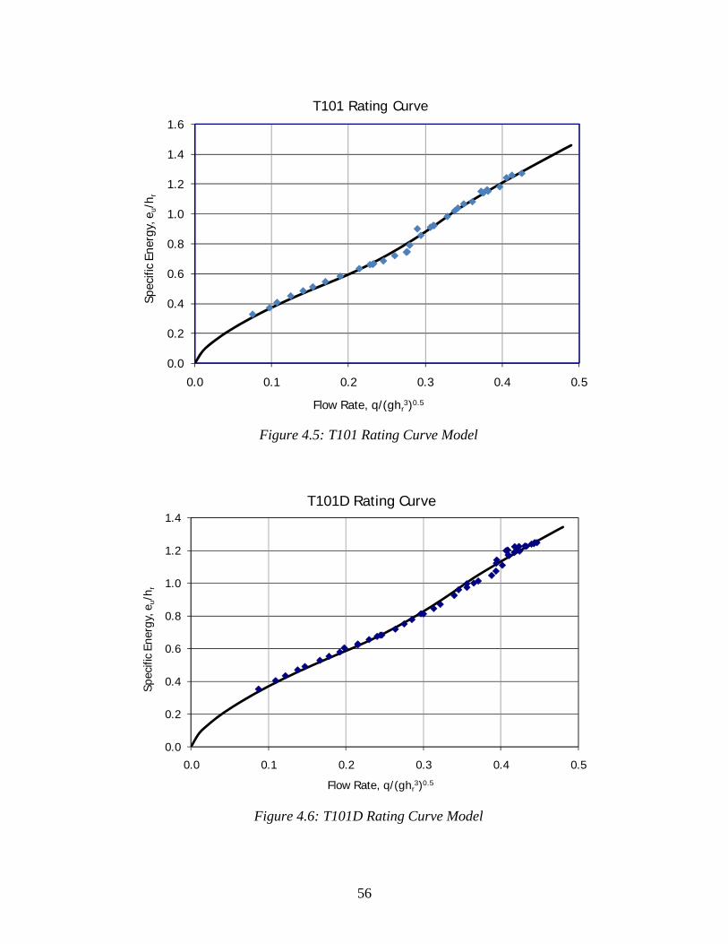
56


Figure 4.6: T101D Rating Curve Model

0.0

0.2

0.4

0.6

0.8

1.0

1.2

1.4

1.6

0.0 0.1 0.2 0.3 0.4 0.5

Spec

ific

Ener

gy, e

u/h r


T101 Rating Curve

0.0

0.2

0.4

0.6

0.8

1.0

1.2

1.4

0.0 0.1 0.2 0.3 0.4 0.5

Spec

ific

Ener

gy, e

u/h r


T101D Rating Curve

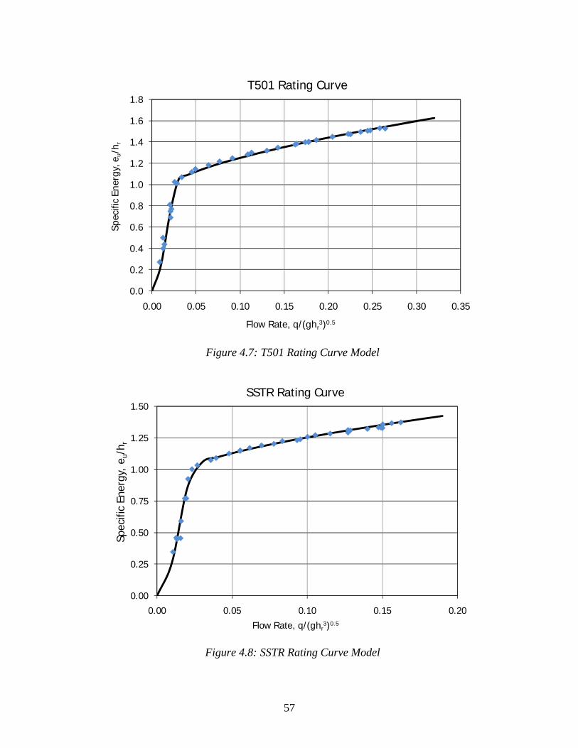
57


Figure 4.8: SSTR Rating Curve Model

0.0

0.2

0.4

0.6

0.8

1.0

1.2

1.4

1.6

1.8

0.00 0.05 0.10 0.15 0.20 0.25 0.30 0.35

Spec

ific

Ener

gy, e

u/h r


T501 Rating Curve

0.00

0.25

0.50

0.75

1.00

1.25

1.50

0.00 0.05 0.10 0.15 0.20

Spec

ific

Ener

gy,

e u/h

r


SSTR Rating Curve

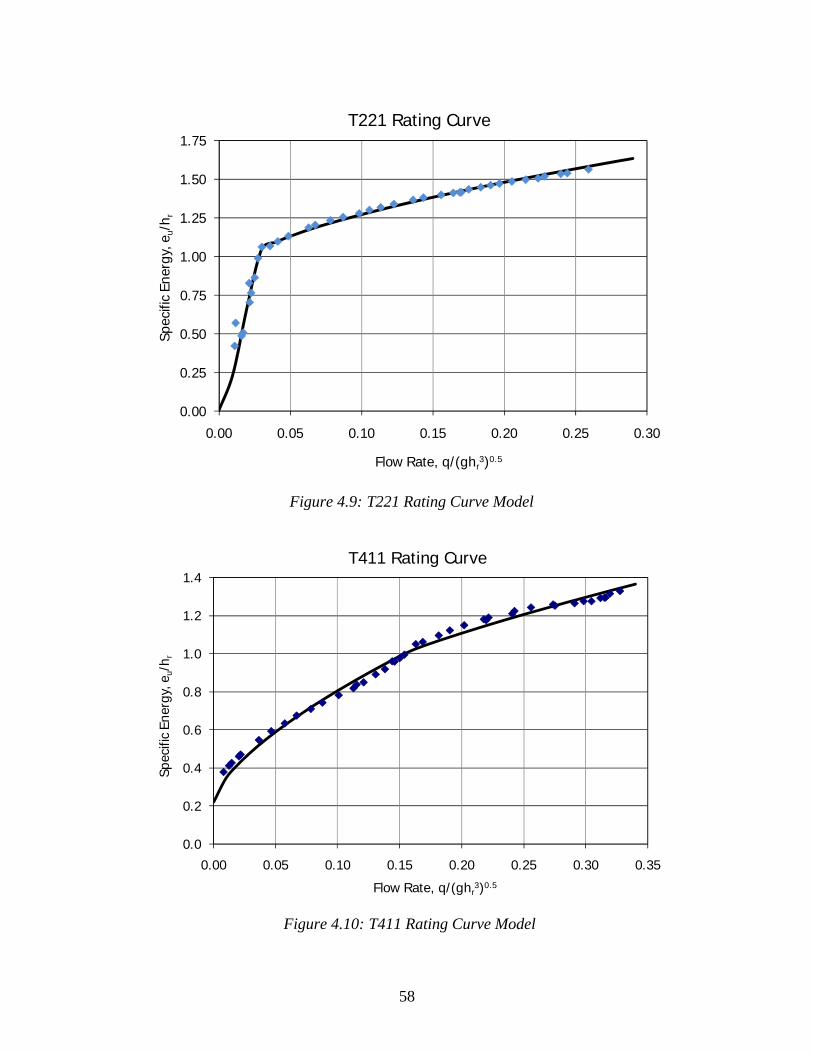
58



0.00

0.25

0.50

0.75

1.00

1.25

1.50

1.75

0.00 0.05 0.10 0.15 0.20 0.25 0.30

Spec

ific

Ener

gy, e

u/h r


T221 Rating Curve

0.0

0.2

0.4

0.6

0.8

1.0

1.2

1.4

0.00 0.05 0.10 0.15 0.20 0.25 0.30 0.35

Spec

ific

Ener

gy, e

u/h r


T411 Rating Curve

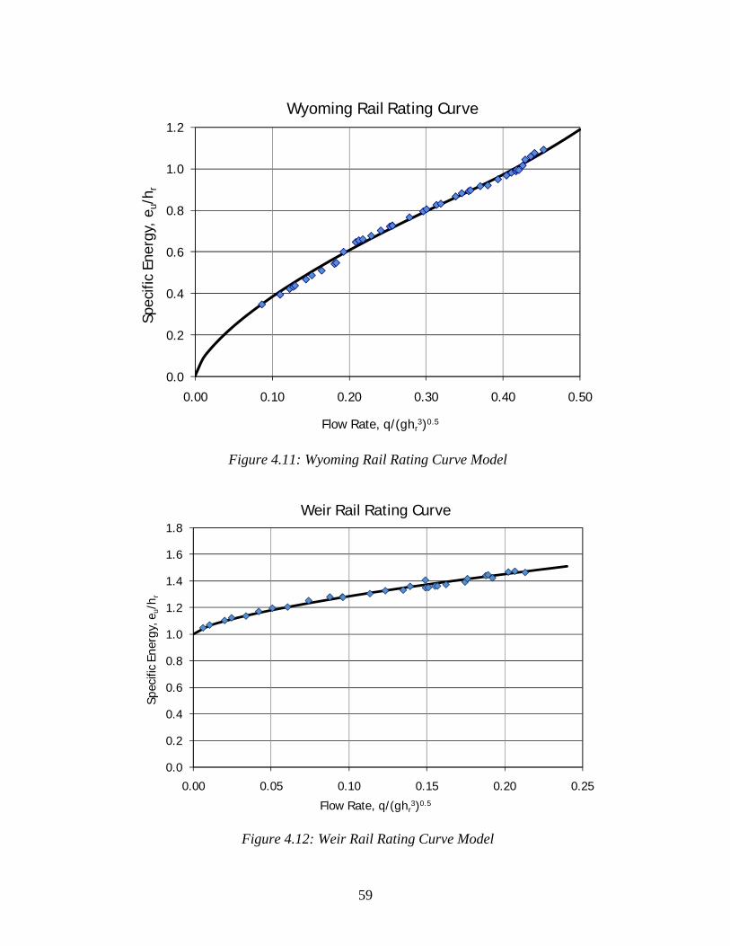
59

Figure 4.11: Wyoming Rail Rating Curve Model

Figure 4.12: Weir Rail Rating Curve Model

0.0

0.2

0.4

0.6

0.8

1.0

1.2

0.00 0.10 0.20 0.30 0.40 0.50

Spec

ific

Ener

gy,

e u/h

r


Wyoming Rail Rating Curve

0.0

0.2

0.4

0.6

0.8

1.0

1.2

1.4

1.6

1.8

0.00 0.05 0.10 0.15 0.20 0.25

Spec

ific

Ener

gy, e

u/h r


Weir Rail Rating Curve

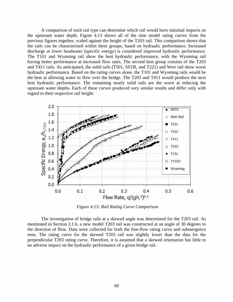
60

A comparison of each rail type can determine which rail would have minimal impacts on the upstream water depth. Figure 4.13 shows all of the nine model rating curves from the previous figures together, scaled against the height of the T203 rail. This comparison shows that the rails can be characterized within three groups, based on hydraulic performance. Increased discharge at lower headwater (specific energy) is considered improved hydraulic performance. The T101 and Wyoming rail show the best hydraulic performance, with the Wyoming rail having better performance at increased flow rates. The second best group consists of the T203 and T411 rails. As anticipated, the solid rails (T501, SSTR, and T221) and Weir rail show worst hydraulic performance. Based on the rating curves alone, the T101 and Wyoming rails would be the best at allowing water to flow over the bridge. The T203 and T411 would produce the next best hydraulic performance. The remaining nearly solid rails are the worst at reducing the upstream water depths. Each of these curves produced very similar results and differ only with regard to their respective rail height.

Figure 4.13: Rail Rating Curve Comparison

The investigation of bridge rails at a skewed angle was determined for the T203 rail. As mentioned in Section 3.1.6, a new model T203 rail was constructed at an angle of 30 degrees to the direction of flow. Data were collected for both the free-flow rating curve and submergence tests. The rating curve for the skewed T203 rail was slightly lower than the data for the perpendicular T203 rating curve. Therefore, it is assumed that a skewed orientation has little to no adverse impact on the hydraulic performance of a given bridge rail.

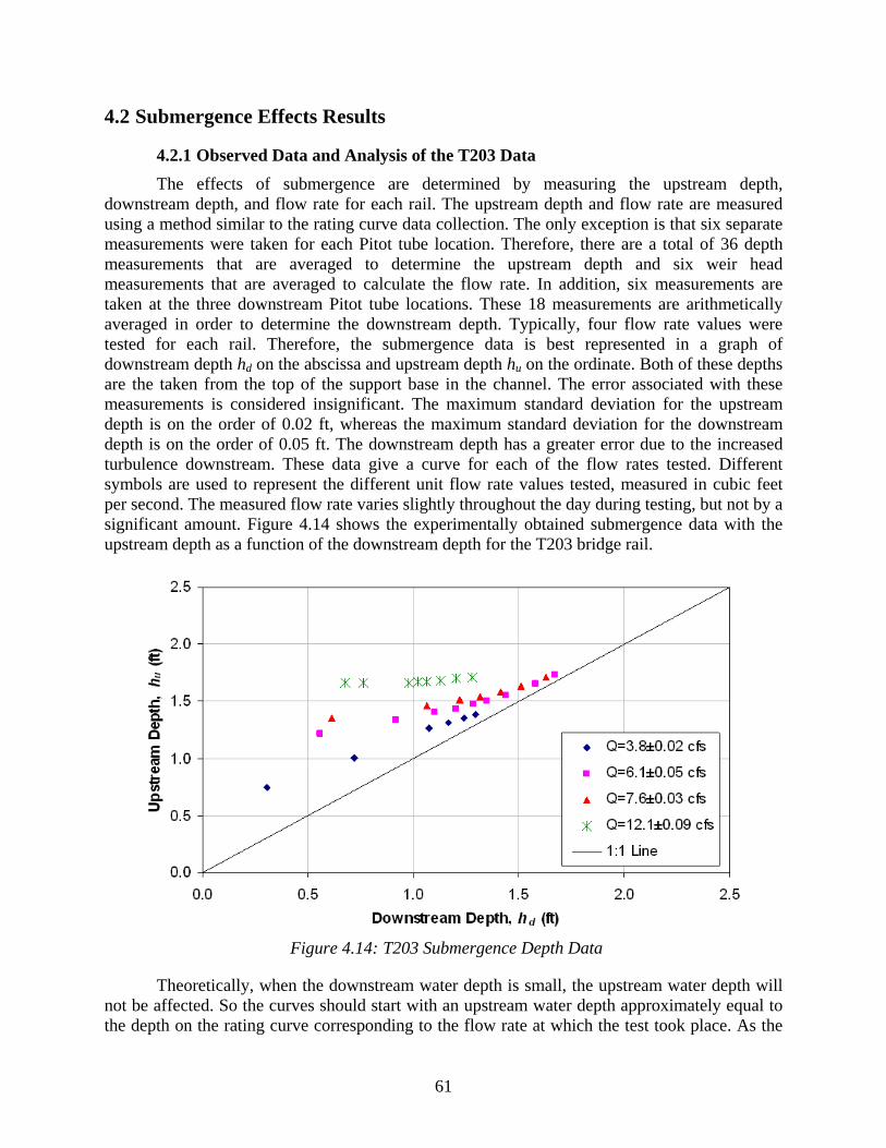
61

4.2 Submergence Effects Results

4.2.1 Observed Data and Analysis of the T203 Data The effects of submergence are determined by measuring the upstream depth, downstream depth, and flow rate for each rail. The upstream depth and flow rate are measured using a method similar to the rating curve data collection. The only exception is that six separate measurements were taken for each Pitot tube location. Therefore, there are a total of 36 depth measurements that are averaged to determine the upstream depth and six weir head measurements that are averaged to calculate the flow rate. In addition, six measurements are taken at the three downstream Pitot tube locations. These 18 measurements are arithmetically averaged in order to determine the downstream depth. Typically, four flow rate values were tested for each rail. Therefore, the submergence data is best represented in a graph of downstream depth hd on the abscissa and upstream depth hu on the ordinate. Both of these depths are the taken from the top of the support base in the channel. The error associated with these measurements is considered insignificant. The maximum standard deviation for the upstream depth is on the order of 0.02 ft, whereas the maximum standard deviation for the downstream depth is on the order of 0.05 ft. The downstream depth has a greater error due to the increased turbulence downstream. These data give a curve for each of the flow rates tested. Different symbols are used to represent the different unit flow rate values tested, measured in cubic feet per second. The measured flow rate varies slightly throughout the day during testing, but not by a significant amount. Figure 4.14 shows the experimentally obtained submergence data with the upstream depth as a function of the downstream depth for the T203 bridge rail.

Figure 4.14: T203 Submergence Depth Data

Theoretically, when the downstream water depth is small, the upstream water depth will not be affected. So the curves should start with an upstream water depth approximately equal to the depth on the rating curve corresponding to the flow rate at which the test took place. As the

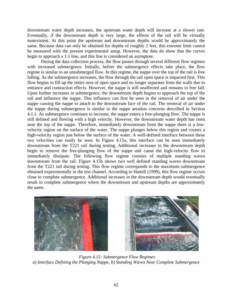
62

downstream water depth increases, the upstream water depth will increase at a slower rate. Eventually, if the downstream depth is very large, the effects of the rail will be virtually nonexistent. At this point the upstream and downstream depths would be approximately the same. Because data can only be obtained for depths of roughly 2 feet, this extreme limit cannot be measured with the present experimental setup. However, the data do show that the curves begin to approach a 1:1 line, and this line is considered an asymptote. During the data collection process, the flow passes through several different flow regimes with increased submergence. Initially, before the submergence effects take place, the flow regime is similar to an unsubmerged flow. In this regime, the nappe over the top of the rail is free falling. As the submergence increases, the flow through the rail open space is impacted first. This flow begins to fill up the entire area of open space and no longer separates from the walls due to entrance and contraction effects. However, the nappe is still unaffected and remains in free fall. Upon further increases in submergence, the downstream depth begins to approach the top of the rail and influence the nappe. This influence can first be seen in the removal of air under the nappe causing the nappe to attach to the downstream face of the rail. The removal of air under the nappe during submergence is similar to the nappe aeration concerns described in Section 4.1.1. As submergence continues to increase, the nappe enters a free-plunging flow. The nappe is still defined and flowing with a high velocity. However, the downstream water depth has risen near the top of the nappe. Therefore, immediately downstream from the nappe there is a low-velocity region on the surface of the water. The nappe plunges below this region and creates a high-velocity region just below the surface of the water. A well-defined interface between these two velocities can easily be seen. In Figure 4.15a, this interface can be seen immediately downstream from the T221 rail during testing. Additional increases in the downstream depth begin to remove the free-plunging flow of the nappe and cause the high-velocity flow to immediately dissipate. The following flow regime consists of multiple standing waves downstream from the rail. Figure 4.15b shows two well defined standing waves downstream from the T221 rail during testing. This flow regime corresponds to the maximum submergence obtained experimentally in the test channel. According to Hamill (1999), this flow regime occurs close to complete submergence. Additional increases in the downstream depth would eventually result in complete submergence where the downstream and upstream depths are approximately the same.

Figure 4.15: Submergence Flow Regimes a) Interface Defining the Plunging Nappe, b) Standing Waves Near Complete Submergence

63

Submergence Results for the T203 Rail With the measured upstream depth, downstream depth, and flow rate values, the Villemonte model and Empirical model can be applied and the model parameters, m and B, can be determined. The calculated model results are compared to the measured flow rate values using the Villemonte equation and Empirical model, which are applied in the form shown below.

m

u

d

ee

qq

⎥⎥⎦

⎤

⎢⎢⎣

⎡⎟⎟⎠

⎞⎜⎜⎝

⎛−=

5.1

1

1 (4.4)

Bq

gh

u

d

r

ee

qq

3

123

1⎟⎟⎠

⎞⎜⎜⎝

⎛⎟⎟⎠

⎞⎜⎜⎝

⎛−= (4.5)

The actual unit flow rate value, q, is measured during testing. The theoretical flow rate produced from the upstream depth, q1, can be determined from the rating curve model using the measured values of hu (which is used to calculate eu) and converting the non-dimensional flow rate into a dimensional flow rate. Therefore, the parameters m and B are the only unknown values in Equations (4.4) and (4.5). These values are determined in much the same way the coefficients for the rating curves were determined. For each averaged point taken, q1 was calculated from the previously determined rating curves and the right hand side of Equations (4.4) and (4.5) were calculated for arbitrary m and B values. The standard error of q/q1 was calculated and minimized by changing the value of m and B using the Solver tool in MS Excel. This gave the value of m and B that result in the minimum error so that when the measured q/q1 and the calculated q/q1 can be plotted against each other, and the results should coincide with a 1:1 line. The results obtained for the T203 rail configuration are shown in Figure 4.16. The solid symbols correspond to the data shown in Figure 4.14 using the Villemonte model results. The open symbols correspond to the Empirical model formulation given by Equation (4.5).

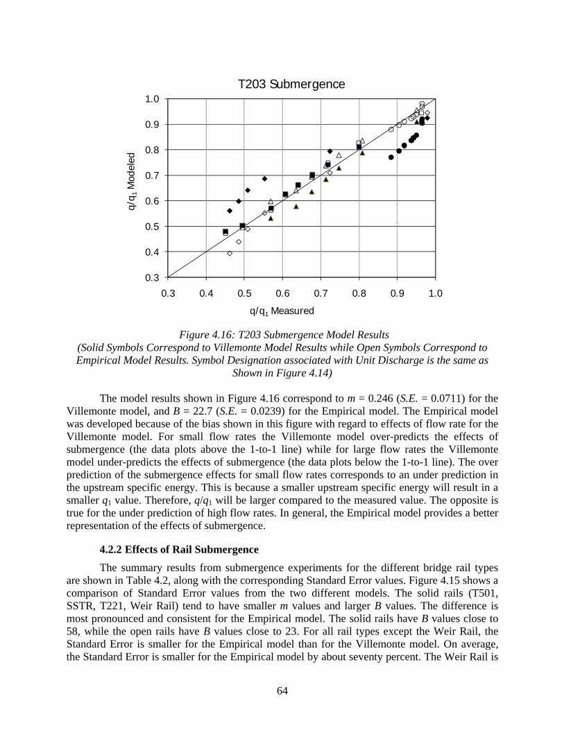
64

Figure 4.16: T203 Submergence Model Results

(Solid Symbols Correspond to Villemonte Model Results while Open Symbols Correspond to Empirical Model Results. Symbol Designation associated with Unit Discharge is the same as

Shown in Figure 4.14) The model results shown in Figure 4.16 correspond to m = 0.246 (S.E. = 0.0711) for the Villemonte model, and B = 22.7 (S.E. = 0.0239) for the Empirical model. The Empirical model was developed because of the bias shown in this figure with regard to effects of flow rate for the Villemonte model. For small flow rates the Villemonte model over-predicts the effects of submergence (the data plots above the 1-to-1 line) while for large flow rates the Villemonte model under-predicts the effects of submergence (the data plots below the 1-to-1 line). The over prediction of the submergence effects for small flow rates corresponds to an under prediction in the upstream specific energy. This is because a smaller upstream specific energy will result in a smaller q1 value. Therefore, q/q1 will be larger compared to the measured value. The opposite is true for the under prediction of high flow rates. In general, the Empirical model provides a better representation of the effects of submergence.

4.2.2 Effects of Rail Submergence The summary results from submergence experiments for the different bridge rail types are shown in Table 4.2, along with the corresponding Standard Error values. Figure 4.15 shows a comparison of Standard Error values from the two different models. The solid rails (T501, SSTR, T221, Weir Rail) tend to have smaller m values and larger B values. The difference is most pronounced and consistent for the Empirical model. The solid rails have B values close to 58, while the open rails have B values close to 23. For all rail types except the Weir Rail, the Standard Error is smaller for the Empirical model than for the Villemonte model. On average, the Standard Error is smaller for the Empirical model by about seventy percent. The Weir Rail is

0.3

0.4

0.5

0.6

0.7

0.8

0.9

1.0

0.3 0.4 0.5 0.6 0.7 0.8 0.9 1.0

q/q 1

Mod

eled

q/q1 Measured

T203 Submergence

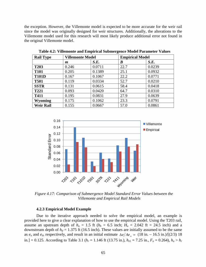
65

the exception. However, the Villemonte model is expected to be more accurate for the weir rail since the model was originally designed for weir structures. Additionally, the alterations to the Villemonte model used for this research will most likely produce additional error not found in the original Villemonte model.

Table 4.2: Villemonte and Empirical Submergence Model Parameter Values Rail Type Villemonte Model Empirical Model m S.E. B S.E. T203 0.246 0.0711 22.7 0.0239 T101 0.205 0.1389 25.1 0.0932 T101D 0.167 0.1067 22.2 0.0771 T501 0.119 0.0334 52.7 0.0210 SSTR 0.131 0.0615 58.4 0.0418 T221 0.093 0.0420 64.7 0.0310 T411 0.195 0.0831 27.9 0.0639 Wyoming 0.175 0.1062 23.3 0.0791 Weir Rail 0.155 0.0667 57.0 0.0861

Figure 4.17: Comparison of Submergence Model Standard Error Values between the

Villemonte and Empirical Rail Models

4.2.3 Empirical Model Example Due to the iterative approach needed to solve the empirical model, an example is provided here to give a clear explanation of how to use the empirical model. Using the T203 rail, assume an upstream depth of hu = 1.5 ft (hb = 6.5 inch; Hu = 2.042 ft = 24.5 inch) and a downstream depth of hd = 1.375 ft (16.5 inch). These values are initially assumed to be the same as eu and ed, respectively, and result in an initial estimate =Δ uAee (18 in. – 16.5 in.)/[(2/3) 18 in.] = 0.125. According to Table 3.1 (hr = 1.146 ft (13.75 in.), hrL = 7.25 in., Fo = 0.264), hu > hr

0.00

0.02

0.04

0.06

0.08

0.10

0.12

0.14

0.16

Stan

dard

Err

or

Villemonte

Empirical

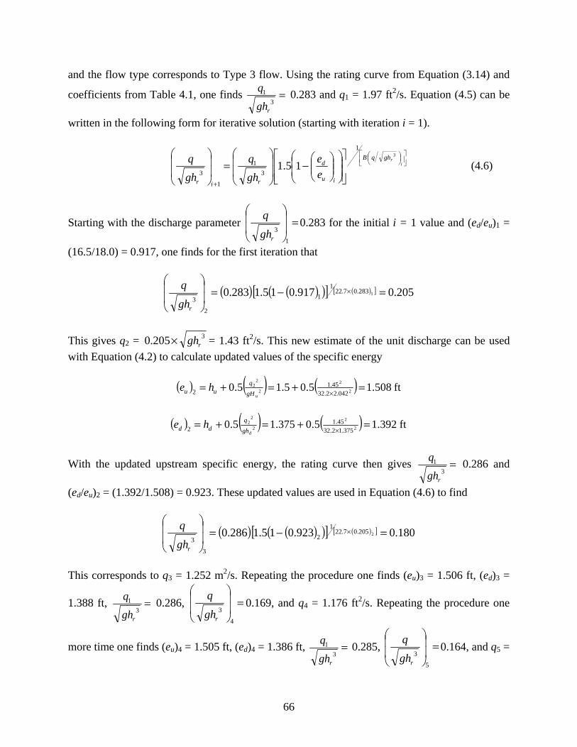
66

and the flow type corresponds to Type 3 flow. Using the rating curve from Equation (3.14) and

coefficients from Table 4.1, one finds =3

1

rgh

q 0.283 and q1 = 1.97 ft2/s. Equation (4.5) can be

written in the following form for iterative solution (starting with iteration i = 1).

⎥⎦⎤

⎢⎣⎡

⎟⎠⎞⎜

⎝⎛

+⎥⎥⎦

⎤

⎢⎢⎣

⎡⎟⎟⎠

⎞⎜⎜⎝

⎛⎟⎟⎠

⎞⎜⎜⎝

⎛−⎟

⎟

⎠

⎞

⎜⎜

⎝

⎛=⎟

⎟

⎠

⎞

⎜⎜

⎝

⎛i

rghqB

iu

d

riree

gh

q

gh

q 31

31

1

315.1 (4.6)

Starting with the discharge parameter =⎟⎟

⎠

⎞

⎜⎜

⎝

⎛

1

3rgh

q 0.283 for the initial i = 1 value and (ed/eu)1 =

(16.5/18.0) = 0.917, one finds for the first iteration that

( ) ( )( )[ ] ( )[ ] 205.0917.015.1283.0 1283.07.221

1

2

3=−=⎟

⎟

⎠

⎞

⎜⎜

⎝

⎛×

rgh

q

This gives q2 = 3205.0 rgh× = 1.43 ft2/s. This new estimate of the unit discharge can be used with Equation (4.2) to calculate updated values of the specific energy

( ) ( ) ( ) ft508.15.05.15.0 2

2

2

22

042.22.3245.1

2 =+=+=×ugH

quu he

( ) ( ) ( ) ft392.15.0375.15.0 2

2

2

22

375.12.3245.1

2 =+=+=×dgh

qdd he

With the updated upstream specific energy, the rating curve then gives =3

1

rgh

q 0.286 and

(ed/eu)2 = (1.392/1.508) = 0.923. These updated values are used in Equation (4.6) to find

( ) ( )( )[ ] ( )[ ] 180.0923.015.1286.0 2205.07.221

2

3

3=−=⎟

⎟

⎠

⎞

⎜⎜

⎝

⎛×

rgh

q

This corresponds to q3 = 1.252 m2/s. Repeating the procedure one finds (eu)3 = 1.506 ft, (ed)3 =

1.388 ft, =3

1

rgh

q 0.286, =⎟⎟

⎠

⎞

⎜⎜

⎝

⎛

4

3rgh

q 0.169, and q4 = 1.176 ft2/s. Repeating the procedure one

more time one finds (eu)4 = 1.505 ft, (ed)4 = 1.386 ft, =3

1

rgh

q 0.285, =⎟⎟

⎠

⎞

⎜⎜

⎝

⎛

5

3rgh

q 0.164, and q5 =

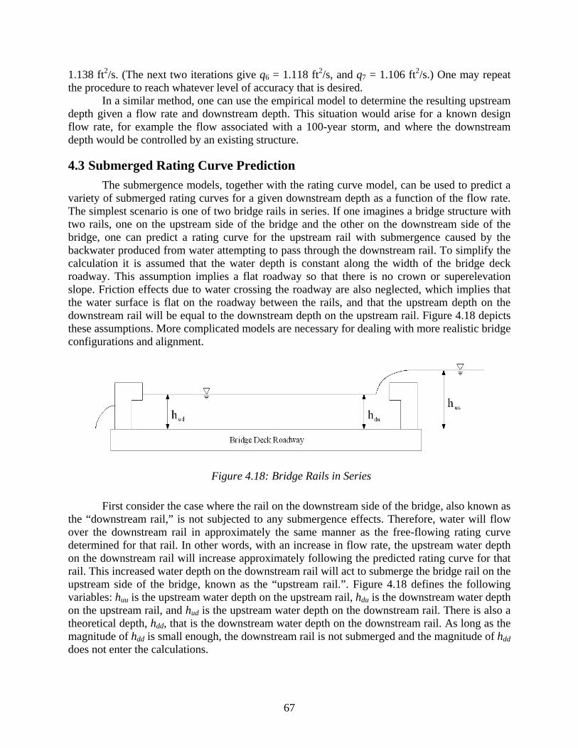
67

1.138 ft2/s. (The next two iterations give q6 = 1.118 ft2/s, and q7 = 1.106 ft2/s.) One may repeat the procedure to reach whatever level of accuracy that is desired. In a similar method, one can use the empirical model to determine the resulting upstream depth given a flow rate and downstream depth. This situation would arise for a known design flow rate, for example the flow associated with a 100-year storm, and where the downstream depth would be controlled by an existing structure.

4.3 Submerged Rating Curve Prediction The submergence models, together with the rating curve model, can be used to predict a variety of submerged rating curves for a given downstream depth as a function of the flow rate. The simplest scenario is one of two bridge rails in series. If one imagines a bridge structure with two rails, one on the upstream side of the bridge and the other on the downstream side of the bridge, one can predict a rating curve for the upstream rail with submergence caused by the backwater produced from water attempting to pass through the downstream rail. To simplify the calculation it is assumed that the water depth is constant along the width of the bridge deck roadway. This assumption implies a flat roadway so that there is no crown or superelevation slope. Friction effects due to water crossing the roadway are also neglected, which implies that the water surface is flat on the roadway between the rails, and that the upstream depth on the downstream rail will be equal to the downstream depth on the upstream rail. Figure 4.18 depicts these assumptions. More complicated models are necessary for dealing with more realistic bridge configurations and alignment.

Figure 4.18: Bridge Rails in Series

First consider the case where the rail on the downstream side of the bridge, also known as the “downstream rail,” is not subjected to any submergence effects. Therefore, water will flow over the downstream rail in approximately the same manner as the free-flowing rating curve determined for that rail. In other words, with an increase in flow rate, the upstream water depth on the downstream rail will increase approximately following the predicted rating curve for that rail. This increased water depth on the downstream rail will act to submerge the bridge rail on the upstream side of the bridge, known as the “upstream rail.”. Figure 4.18 defines the following variables: huu is the upstream water depth on the upstream rail, hdu is the downstream water depth on the upstream rail, and hud is the upstream water depth on the downstream rail. There is also a theoretical depth, hdd, that is the downstream water depth on the downstream rail. As long as the magnitude of hdd is small enough, the downstream rail is not submerged and the magnitude of hdd does not enter the calculations.

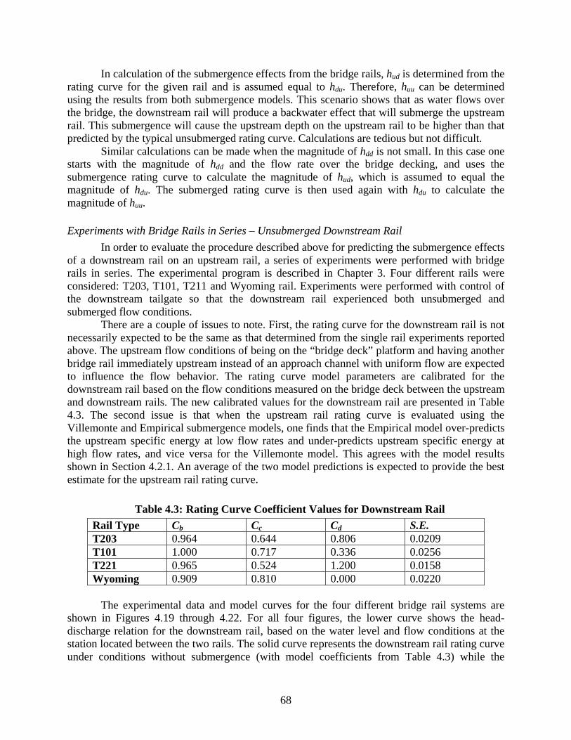
68

In calculation of the submergence effects from the bridge rails, hud is determined from the rating curve for the given rail and is assumed equal to hdu. Therefore, huu can be determined using the results from both submergence models. This scenario shows that as water flows over the bridge, the downstream rail will produce a backwater effect that will submerge the upstream rail. This submergence will cause the upstream depth on the upstream rail to be higher than that predicted by the typical unsubmerged rating curve. Calculations are tedious but not difficult.

Similar calculations can be made when the magnitude of hdd is not small. In this case one starts with the magnitude of hdd and the flow rate over the bridge decking, and uses the submergence rating curve to calculate the magnitude of hud, which is assumed to equal the magnitude of hdu. The submerged rating curve is then used again with hdu to calculate the magnitude of huu.

Experiments with Bridge Rails in Series – Unsubmerged Downstream Rail In order to evaluate the procedure described above for predicting the submergence effects of a downstream rail on an upstream rail, a series of experiments were performed with bridge rails in series. The experimental program is described in Chapter 3. Four different rails were considered: T203, T101, T211 and Wyoming rail. Experiments were performed with control of the downstream tailgate so that the downstream rail experienced both unsubmerged and submerged flow conditions. There are a couple of issues to note. First, the rating curve for the downstream rail is not necessarily expected to be the same as that determined from the single rail experiments reported above. The upstream flow conditions of being on the “bridge deck” platform and having another bridge rail immediately upstream instead of an approach channel with uniform flow are expected to influence the flow behavior. The rating curve model parameters are calibrated for the downstream rail based on the flow conditions measured on the bridge deck between the upstream and downstream rails. The new calibrated values for the downstream rail are presented in Table 4.3. The second issue is that when the upstream rail rating curve is evaluated using the Villemonte and Empirical submergence models, one finds that the Empirical model over-predicts the upstream specific energy at low flow rates and under-predicts upstream specific energy at high flow rates, and vice versa for the Villemonte model. This agrees with the model results shown in Section 4.2.1. An average of the two model predictions is expected to provide the best estimate for the upstream rail rating curve.

Table 4.3: Rating Curve Coefficient Values for Downstream Rail Rail Type Cb Cc Cd S.E. T203 0.964 0.644 0.806 0.0209 T101 1.000 0.717 0.336 0.0256 T221 0.965 0.524 1.200 0.0158 Wyoming 0.909 0.810 0.000 0.0220

The experimental data and model curves for the four different bridge rail systems are shown in Figures 4.19 through 4.22. For all four figures, the lower curve shows the head-discharge relation for the downstream rail, based on the water level and flow conditions at the station located between the two rails. The solid curve represents the downstream rail rating curve under conditions without submergence (with model coefficients from Table 4.3) while the

69

diamond symbols represent the measured data. The upper curve corresponds to conditions upstream of the rail system. The dashed line is calculated using the average of the Villemonte and Empirical submergence models (with model coefficients from Tables 4.1 and 4.2), and the triangle symbols represent the measured data. Based on results for the T101 and Wyoming rail systems, it appears that the calculation method over-predicts submergence effects for rails with significant open space. However, the method predictions are considered good for the T203 and T211 rails, which represent rails of intermediate and no (very limited) open space, respectively.

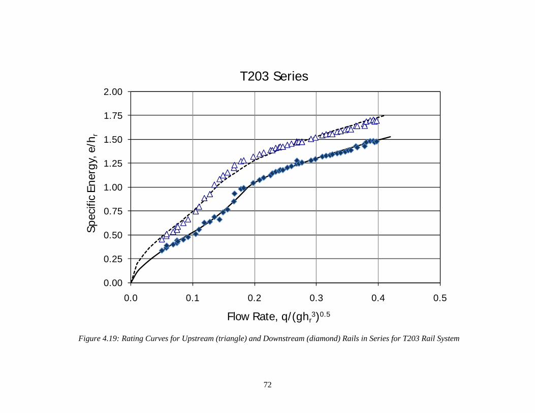
72

Figure 4.19: Rating Curves for Upstream (triangle) and Downstream (diamond) Rails in Series for T203 Rail System

0.00

0.25

0.50

0.75

1.00

1.25

1.50

1.75

2.00

0.0 0.1 0.2 0.3 0.4 0.5

Spec

ific

Ener

gy, e

/hr


T203 Series

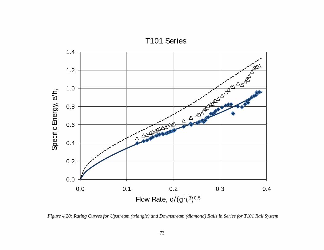
73


0.0

0.2

0.4

0.6

0.8

1.0

1.2

1.4

0.0 0.1 0.2 0.3 0.4

Spec

ific

Ener

gy, e

/hr


T101 Series

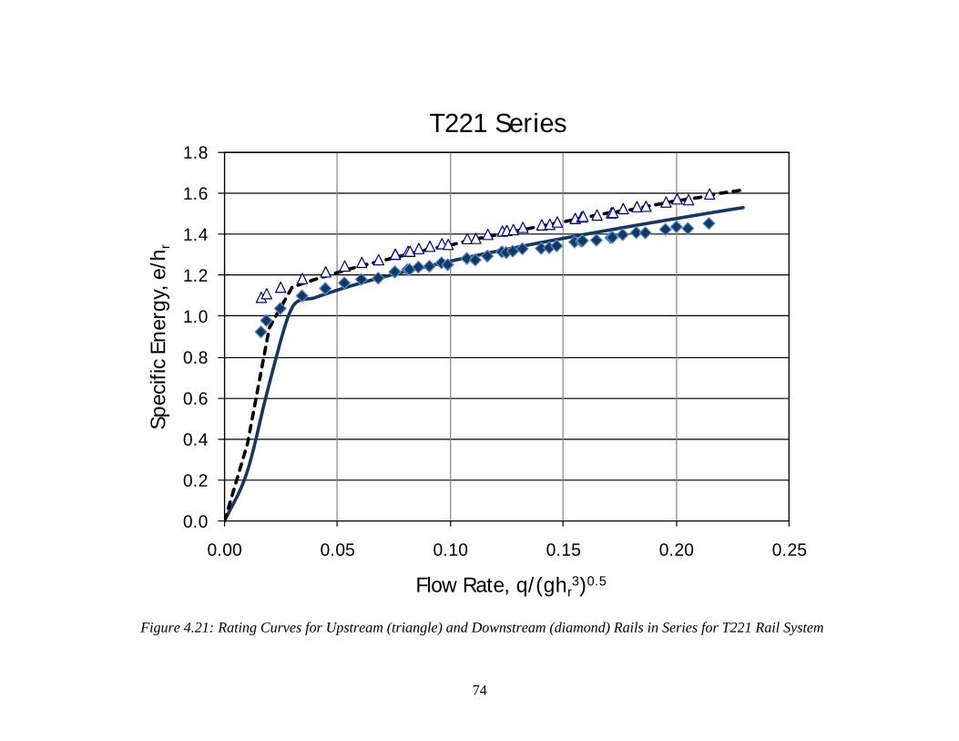
74


0.0

0.2

0.4

0.6

0.8

1.0

1.2

1.4

1.6

1.8

0.00 0.05 0.10 0.15 0.20 0.25

Spec

ific

Ener

gy, e

/hr


T221 Series

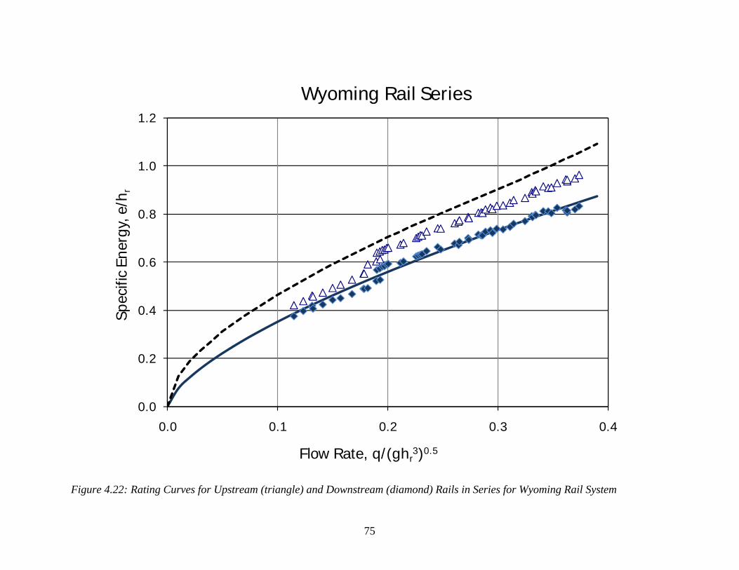
75

Figure 4.22: Rating Curves for Upstream (triangle) and Downstream (diamond) Rails in Series for Wyoming Rail System

0.0

0.2

0.4

0.6

0.8

1.0

1.2

0.0 0.1 0.2 0.3 0.4

Spec

ific

Ener

gy, e

/hr


Wyoming Rail Series

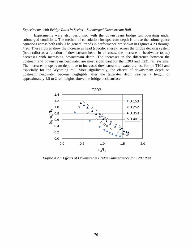
76

Experiments with Bridge Rails in Series – Submerged Downstream Rail Experiments were also performed with the downstream bridge rail operating under submerged conditions. The method of calculation for upstream depth is to use the submergence equations across both rails. The general trends in performance are shown in Figures 4.23 through 4.26. These figures show the increase in head (specific energy) across the bridge decking system (both rails) as a function of downstream head. In all cases, the increase in headwater (eu-ed) decreases with increasing downstream depth. The increases in the difference between the upstream and downstream headwater are most significant for the T203 and T221 rail systems. The increases in upstream depth due to increased downstream tailwater are less for the T101 and especially for the Wyoming rail. Most significantly, the effects of downstream depth on upstream headwater become negligible after the tailwater depth reaches a height of approximately 1.5 to 2 rail heights above the bridge deck surface.

Figure 4.23: Effects of Downstream Bridge Submergence for T203 Rail

0.0

0.2

0.4

0.6

0.8

1.0

1.2

1.4

0.0 0.5 1.0 1.5 2.0

(eu-

e d)/

h r

ed/hr

T203

0.153

0.252

0.353

0.401

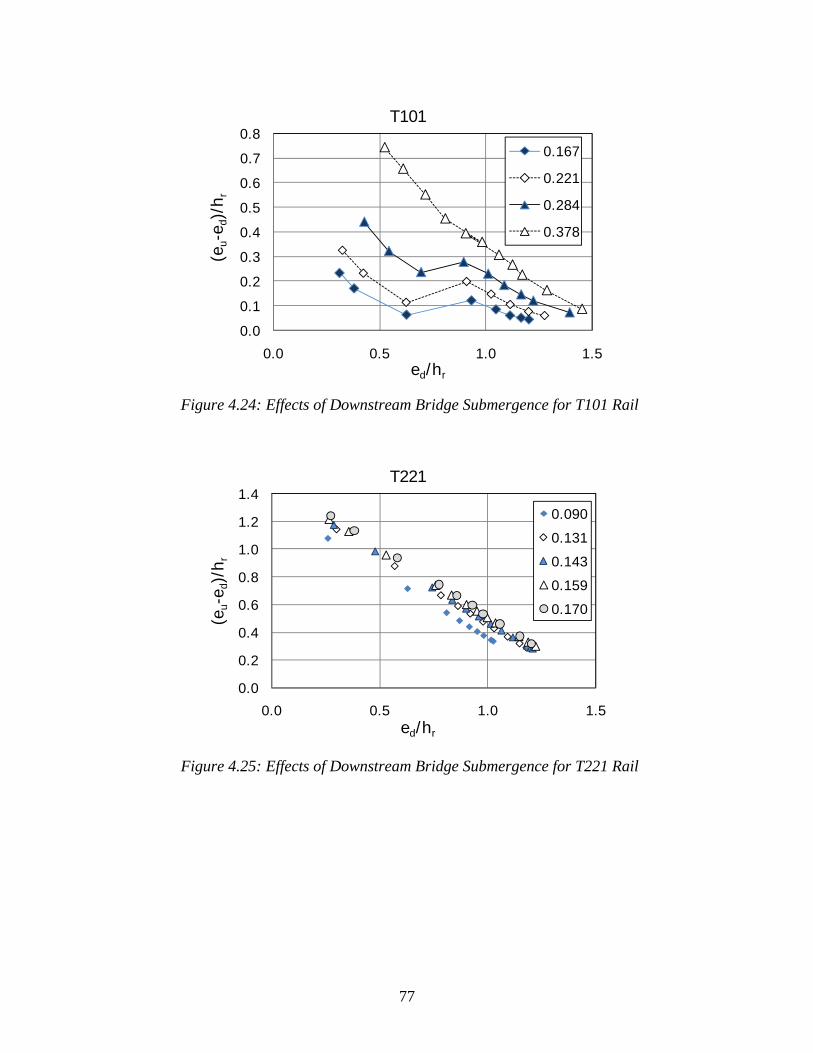
77



0.0

0.1

0.2

0.3

0.4

0.5

0.6

0.7

0.8

0.0 0.5 1.0 1.5

(eu-

e d)/

h r

ed/hr

T101

0.167

0.221

0.284

0.378

0.0

0.2

0.4

0.6

0.8

1.0

1.2

1.4

0.0 0.5 1.0 1.5

(eu-

e d)/

h r

ed/hr

T221

0.090

0.131

0.143

0.159

0.170

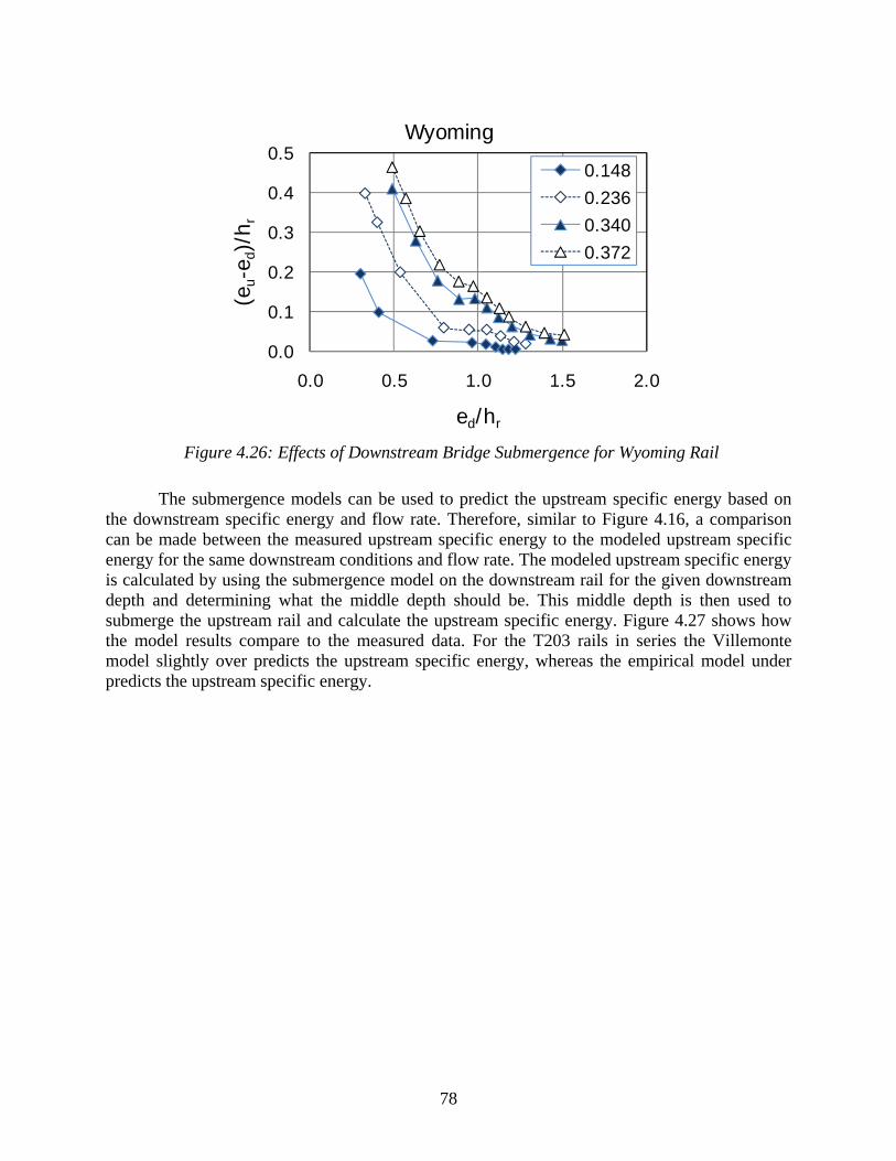
78

Figure 4.26: Effects of Downstream Bridge Submergence for Wyoming Rail

The submergence models can be used to predict the upstream specific energy based on the downstream specific energy and flow rate. Therefore, similar to Figure 4.16, a comparison can be made between the measured upstream specific energy to the modeled upstream specific energy for the same downstream conditions and flow rate. The modeled upstream specific energy is calculated by using the submergence model on the downstream rail for the given downstream depth and determining what the middle depth should be. This middle depth is then used to submerge the upstream rail and calculate the upstream specific energy. Figure 4.27 shows how the model results compare to the measured data. For the T203 rails in series the Villemonte model slightly over predicts the upstream specific energy, whereas the empirical model under predicts the upstream specific energy.

0.0

0.1

0.2

0.3

0.4

0.5

0.0 0.5 1.0 1.5 2.0

(eu-

e d)/

h r

ed/hr

Wyoming

0.1480.2360.3400.372

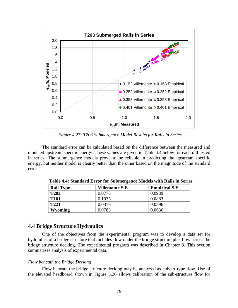
79

Figure 4.27: T203 Submergence Model Results for Rails in Series

The standard error can be calculated based on the difference between the measured and modeled upstream specific energy. These values are given in Table 4.4 below for each rail tested in series. The submergence models prove to be reliable in predicting the upstream specific energy, but neither model is clearly better than the other based on the magnitude of the standard error.

Table 4.4: Standard Error for Submergence Models with Rails in Series Rail Type Villemonte S.E. Empirical S.E. T203 0.0773 0.0939 T101 0.1035 0.0883 T221 0.0378 0.0396 Wyoming 0.0783 0.0636

4.4 Bridge Structure Hydraulics One of the objectives from the experimental program was to develop a data set for

hydraulics of a bridge structure that includes flow under the bridge structure plus flow across the bridge structure decking. The experimental program was described in Chapter 3. This section summarizes analysis of experimental data.

Flow beneath the Bridge Decking Flow beneath the bridge structure decking may be analyzed as culvert-type flow. Use of the elevated headboard shown in Figure 3.26 allows calibration of the sub-structure flow for

T203 Submerged Rails in Series

0.0

0.2

0.4

0.6

0.8

1.0

1.2

1.4

1.6

1.8

2.0

0.0 0.5 1.0 1.5 2.0

euu/hr Measured

e uu/h

r Mod

eled

0.153 Villemonte 0.153 Empirical




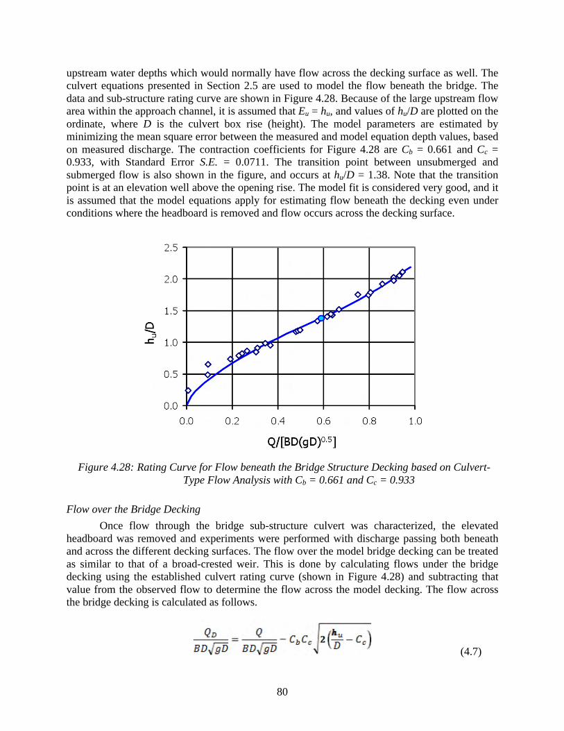
80

upstream water depths which would normally have flow across the decking surface as well. The

culvert equations presented in Section 2.5 are used to model the flow beneath the bridge. The

data and sub-structure rating curve are shown in Figure 4.28. Because of the large upstream flow

area within the approach channel, it is assumed that Eu = hu, and values of hu/D are plotted on the

ordinate, where D is the culvert box rise (height). The model parameters are estimated by

minimizing the mean square error between the measured and model equation depth values, based

on measured discharge. The contraction coefficients for Figure 4.28 are Cb = 0.661 and Cc =

0.933, with Standard Error S.E. = 0.0711. The transition point between unsubmerged and

submerged flow is also shown in the figure, and occurs at hu/D = 1.38. Note that the transition

point is at an elevation well above the opening rise. The model fit is considered very good, and it

is assumed that the model equations apply for estimating flow beneath the decking even under

conditions where the headboard is removed and flow occurs across the decking surface.

Figure 4.28: Rating Curve for Flow beneath the Bridge Structure Decking based on Culvert-

Type Flow Analysis with Cb = 0.661 and Cc = 0.933

Flow over the Bridge Decking

Once flow through the bridge sub-structure culvert was characterized, the elevated

headboard was removed and experiments were performed with discharge passing both beneath

and across the different decking surfaces. The flow over the model bridge decking can be treated

as similar to that of a broad-crested weir. This is done by calculating flows under the bridge

decking using the established culvert rating curve (shown in Figure 4.28) and subtracting that

value from the observed flow to determine the flow across the model decking. The flow across

the bridge decking is calculated as follows.

(4.7)

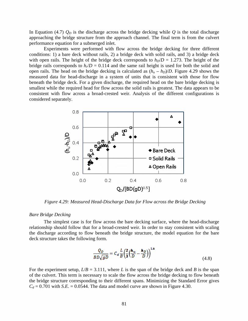
81

In Equation (4.7) QD is the discharge across the bridge decking while Q is the total discharge

approaching the bridge structure from the approach channel. The final term is from the culvert

performance equation for a submerged inlet.

Experiments were performed with flow across the bridge decking for three different

conditions: 1) a bare deck without rails, 2) a bridge deck with solid rails, and 3) a bridge deck

with open rails. The height of the bridge deck corresponds to hD/D = 1.273. The height of the

bridge rails corresponds to hr/D = 0.114 and the same rail height is used for both the solid and

open rails. The head on the bridge decking is calculated as (hu – hD)/D. Figure 4.29 shows the

measured data for head-discharge in a system of units that is consistent with those for flow

beneath the bridge deck. For a given discharge, the required head on the bare bridge decking is

smallest while the required head for flow across the solid rails is greatest. The data appears to be

consistent with flow across a broad-crested weir. Analysis of the different configurations is

considered separately.

Figure 4.29: Measured Head-Discharge Data for Flow across the Bridge Decking

Bare Bridge Decking

The simplest case is for flow across the bare decking surface, where the head-discharge

relationship should follow that for a broad-crested weir. In order to stay consistent with scaling

the discharge according to flow beneath the bridge structure, the model equation for the bare

deck structure takes the following form.

(4.8)

For the experiment setup, L/B = 3.111, where L is the span of the bridge deck and B is the span

of the culvert. This term is necessary to scale the flow across the bridge decking to flow beneath

the bridge structure corresponding to their different spans. Minimizing the Standard Error gives

Cd = 0.701 with S.E. = 0.0544. The data and model curve are shown in Figure 4.30.

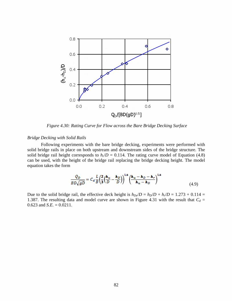
82

Figure 4.30: Rating Curve for Flow across the Bare Bridge Decking Surface

Bridge Decking with Solid Rails

Following experiments with the bare bridge decking, experiments were performed with

solid bridge rails in place on both upstream and downstream sides of the bridge structure. The

solid bridge rail height corresponds to hr/D = 0.114. The rating curve model of Equation (4.8)

can be used, with the height of the bridge rail replacing the bridge decking height. The model

equation takes the form

(4.9)

Due to the solid bridge rail, the effective deck height is hDe/D = hD/D + hr/D = 1.273 + 0.114 =

1.387. The resulting data and model curve are shown in Figure 4.31 with the result that Cd =

0.623 and S.E. = 0.0211.

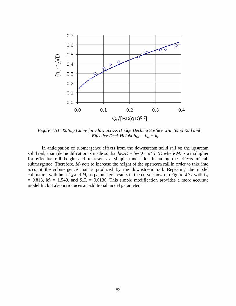
83

Figure 4.31: Rating Curve for Flow across Bridge Decking Surface with Solid Rail and

Effective Deck Height hDe = hD + hr

In anticipation of submergence effects from the downstream solid rail on the upstream solid rail, a simple modification is made so that hDe/D = hD/D + Mr hr/D where Mr is a multiplier for effective rail height and represents a simple model for including the effects of rail submergence. Therefore, Mr acts to increase the height of the upstream rail in order to take into account the submergence that is produced by the downstream rail. Repeating the model calibration with both Cd and Mr as parameters results in the curve shown in Figure 4.32 with Cd = 0.813, Mr = 1.549, and S.E. = 0.0130. This simple modification provides a more accurate model fit, but also introduces an additional model parameter.

0.0

0.1

0.2

0.3

0.4

0.5

0.6

0.7

0.0 0.1 0.2 0.3 0.4

(hu-

h D)/

D

QD/[BD(gD)0.5]

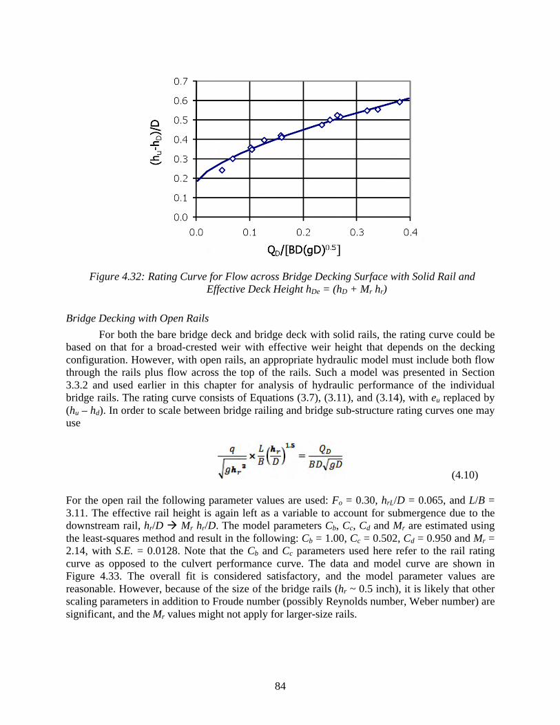
84

Figure 4.32: Rating Curve for Flow across Bridge Decking Surface with Solid Rail and

Effective Deck Height hDe = (hD + Mr hr)

Bridge Decking with Open Rails

For both the bare bridge deck and bridge deck with solid rails, the rating curve could be

based on that for a broad-crested weir with effective weir height that depends on the decking

configuration. However, with open rails, an appropriate hydraulic model must include both flow

through the rails plus flow across the top of the rails. Such a model was presented in Section

3.3.2 and used earlier in this chapter for analysis of hydraulic performance of the individual

bridge rails. The rating curve consists of Equations (3.7), (3.11), and (3.14), with eu replaced by

(hu – hd). In order to scale between bridge railing and bridge sub-structure rating curves one may

use

(4.10)

For the open rail the following parameter values are used: Fo = 0.30, hrL/D = 0.065, and L/B =

3.11. The effective rail height is again left as a variable to account for submergence due to the

downstream rail, hr/D Mr hr/D. The model parameters Cb, Cc, Cd and Mr are estimated using

the least-squares method and result in the following: Cb = 1.00, Cc = 0.502, Cd = 0.950 and Mr =

2.14, with S.E. = 0.0128. Note that the Cb and Cc parameters used here refer to the rail rating

curve as opposed to the culvert performance curve. The data and model curve are shown in

Figure 4.33. The overall fit is considered satisfactory, and the model parameter values are

reasonable. However, because of the size of the bridge rails (hr ~ 0.5 inch), it is likely that other

scaling parameters in addition to Froude number (possibly Reynolds number, Weber number) are

significant, and the Mr values might not apply for larger-size rails.

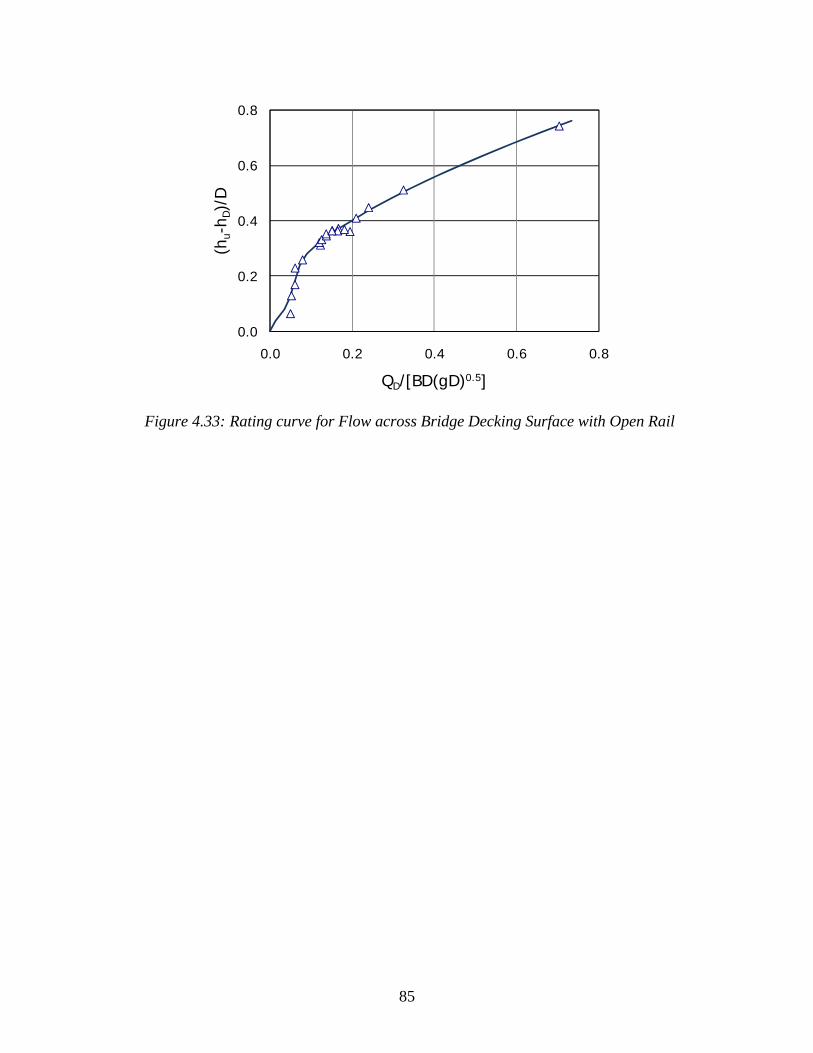
85

Figure 4.33: Rating curve for Flow across Bridge Decking Surface with Open Rail

0.0

0.2

0.4

0.6

0.8

0.0 0.2 0.4 0.6 0.8

(hu-

h D)/

D

QD/[BD(gD)0.5]

86

87

Chapter 5. HEC-RAS Bridge Method Alterations

It is important to develop procedures to include bridge rail hydraulic data in floodplain

analysis models such as HEC-RAS. This chapter describes the equations used by HEC-RAS in

determining the water surface profile around bridge structures under a high flow regime. High

flow is defined as flows in which the water surface comes into contact with the maximum low

chord of the bridge deck. There are two high flow methods available for calculation: the energy

equation and the pressure/weir flow equations. Before these methods are discussed, an overview

of the bridge structure calculations is given. Additionally, procedures are suggested for including

the bridge rail rating curve and submergence data discussed in Chapter 4 in HEC-RAS

simulations of bridge effects on floodplain elevations. Finally, a HEC-RAS model application to

the simple bridge structure described in this report is considered.

5.1 Bridge Rail Computation Introduction

HEC-RAS uses four user defined cross sections in the computations of energy losses due

to the bridge structure. These are shown in Figure 5.1 below. The contraction reach coefficient

(CR) and expansion reach coefficient (ER) can be defined by the user and are used to calculate

the contraction reach length (Lc) and expansion reach length (Le), respectively. In addition, RAS

creates two interpolated cross sections inside the bridge structure, shown in Figure 5.2.

Computations start from the downstream end (cross section 1) and continue upstream until cross

section 4 is reached through a total of six cross sections.

Figure 5.1: Four User-Defined Cross Sections (source: HEC, 2002)

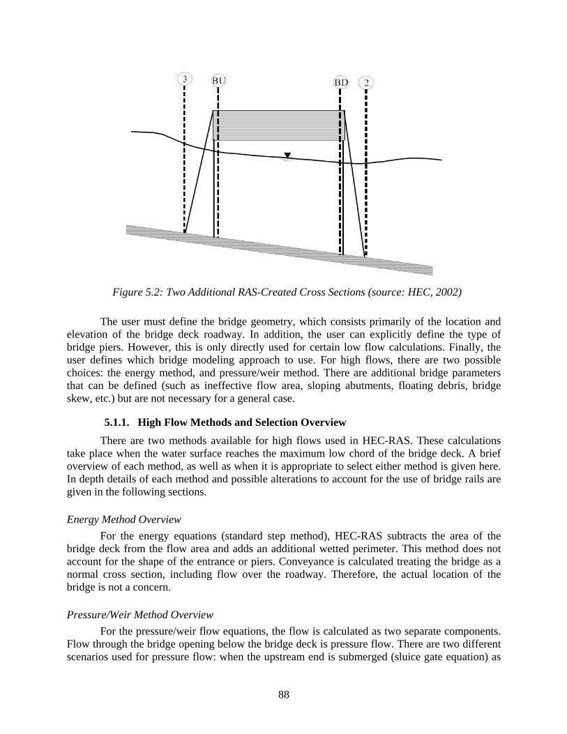
88

Figure 5.2: Two Additional RAS-Created Cross Sections (source: HEC, 2002)

The user must define the bridge geometry, which consists primarily of the location and elevation of the bridge deck roadway. In addition, the user can explicitly define the type of bridge piers. However, this is only directly used for certain low flow calculations. Finally, the user defines which bridge modeling approach to use. For high flows, there are two possible choices: the energy method, and pressure/weir method. There are additional bridge parameters that can be defined (such as ineffective flow area, sloping abutments, floating debris, bridge skew, etc.) but are not necessary for a general case.

5.1.1. High Flow Methods and Selection Overview There are two methods available for high flows used in HEC-RAS. These calculations take place when the water surface reaches the maximum low chord of the bridge deck. A brief overview of each method, as well as when it is appropriate to select either method is given here. In depth details of each method and possible alterations to account for the use of bridge rails are given in the following sections.

Energy Method Overview For the energy equations (standard step method), HEC-RAS subtracts the area of the bridge deck from the flow area and adds an additional wetted perimeter. This method does not account for the shape of the entrance or piers. Conveyance is calculated treating the bridge as a normal cross section, including flow over the roadway. Therefore, the actual location of the bridge is not a concern.

Pressure/Weir Method Overview For the pressure/weir flow equations, the flow is calculated as two separate components. Flow through the bridge opening below the bridge deck is pressure flow. There are two different scenarios used for pressure flow: when the upstream end is submerged (sluice gate equation) as

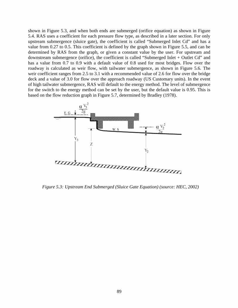
89

shown in Figure 5.3, and when both ends are submerged (orifice equation) as shown in Figure

5.4. RAS uses a coefficient for each pressure flow type, as described in a later section. For only

upstream submergence (sluice gate), the coefficient is called “Submerged Inlet Cd” and has a

value from 0.27 to 0.5. This coefficient is defined by the graph shown in Figure 5.5, and can be

determined by RAS from the graph, or given a constant value by the user. For upstream and

downstream submergence (orifice), the coefficient is called “Submerged Inlet + Outlet Cd” and

has a value from 0.7 to 0.9 with a default value of 0.8 used for most bridges. Flow over the

roadway is calculated as weir flow, with tailwater submergence, as shown in Figure 5.6. The

weir coefficient ranges from 2.5 to 3.1 with a recommended value of 2.6 for flow over the bridge

deck and a value of 3.0 for flow over the approach roadway (US Customary units). In the event

of high tailwater submergence, RAS will default to the energy method. The level of submergence

for the switch to the energy method can be set by the user, but the default value is 0.95. This is

based on the flow reduction graph in Figure 5.7, determined by Bradley (1978).

Figure 5.3: Upstream End Submerged (Sluice Gate Equation) (source: HEC, 2002)

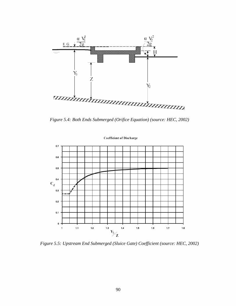
90

Figure 5.4: Both Ends Submerged (Orifice Equation) (source: HEC, 2002)

Figure 5.5: Upstream End Submerged (Sluice Gate) Coefficient (source: HEC, 2002)

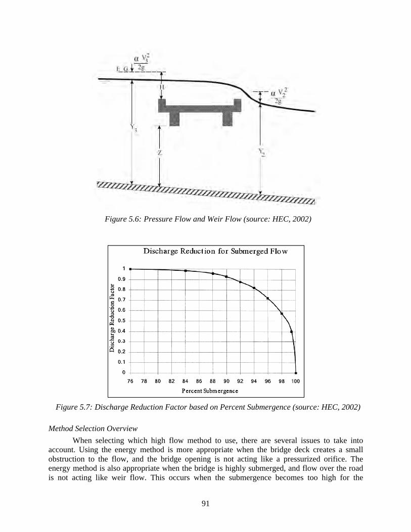
91

Figure 5.6: Pressure Flow and Weir Flow (source: HEC, 2002)

Figure 5.7: Discharge Reduction Factor based on Percent Submergence (source: HEC, 2002)

Method Selection Overview

When selecting which high flow method to use, there are several issues to take into

account. Using the energy method is more appropriate when the bridge deck creates a small

obstruction to the flow, and the bridge opening is not acting like a pressurized orifice. The

energy method is also appropriate when the bridge is highly submerged, and flow over the road

is not acting like weir flow. This occurs when the submergence becomes too high for the

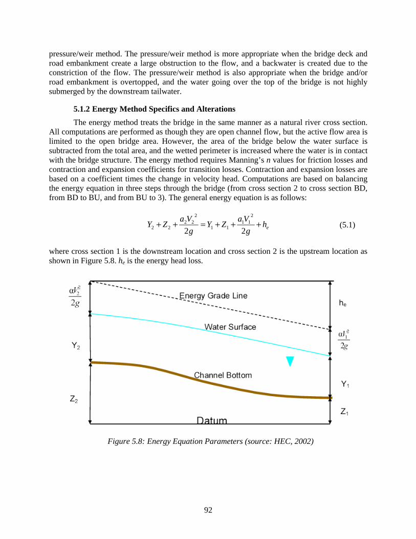
92

pressure/weir method. The pressure/weir method is more appropriate when the bridge deck and road embankment create a large obstruction to the flow, and a backwater is created due to the constriction of the flow. The pressure/weir method is also appropriate when the bridge and/or road embankment is overtopped, and the water going over the top of the bridge is not highly submerged by the downstream tailwater.

5.1.2 Energy Method Specifics and Alterations

The energy method treats the bridge in the same manner as a natural river cross section. All computations are performed as though they are open channel flow, but the active flow area is limited to the open bridge area. However, the area of the bridge below the water surface is subtracted from the total area, and the wetted perimeter is increased where the water is in contact with the bridge structure. The energy method requires Manning’s n values for friction losses and contraction and expansion coefficients for transition losses. Contraction and expansion losses are based on a coefficient times the change in velocity head. Computations are based on balancing the energy equation in three steps through the bridge (from cross section 2 to cross section BD, from BD to BU, and from BU to 3). The general energy equation is as follows:

ehg

VaZYg

VaZY +++=++22

211

11

222

22 (5.1)

where cross section 1 is the downstream location and cross section 2 is the upstream location as shown in Figure 5.8. he is the energy head loss.

Figure 5.8: Energy Equation Parameters (source: HEC, 2002)

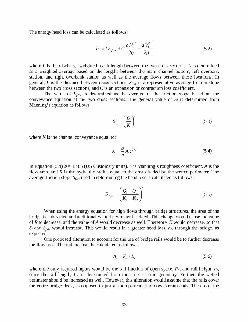
93

The energy head loss can be calculated as follows:

g

Vag

VaCLSh avfe 22

211

222

, −+= (5.2)

where L is the discharge weighted reach length between the two cross sections. L is determined as a weighted average based on the lengths between the main channel bottom, left overbank station, and right overbank station as well as the average flows between these locations. In general, L is the distance between cross sections. Sf,av is a representative average friction slope between the two cross sections, and C is an expansion or contraction loss coefficient. The value of Sf,av is determined as the average of the friction slope based on the conveyance equation at the two cross sections. The general value of Sf is determined from Manning’s equation as follows:

2

⎟⎠⎞

⎜⎝⎛=

KQS f (5.3)

where K is the channel conveyance equal to:

3/2ARn

K φ= (5.4)

In Equation (5.4) φ = 1.486 (US Customary units), n is Manning’s roughness coefficient, A is the flow area, and R is the hydraulic radius equal to the area divided by the wetted perimeter. The average friction slope Sf,av used in determining the head loss is calculated as follows:

2

21

21, ⎟⎟

⎠

⎞⎜⎜⎝

⎛++

=KKQQS avf (5.5)

When using the energy equation for high flows through bridge structures, the area of the bridge is subtracted and additional wetted perimeter is added. This change would cause the value of R to decrease, and the value of A would decrease as well. Therefore, K would decrease, so that Sf and Sf,av would increase. This would result in a greater head loss, he, through the bridge, as expected. One proposed alteration to account for the use of bridge rails would be to further decrease the flow area. The rail area can be calculated as follows: rror LhFA = (5.6) where the only required inputs would be the rail fraction of open space, Fo, and rail height, hr, since the rail length, Lr, is determined from the cross section geometry. Further, the wetted perimeter should be increased as well. However, this alteration would assume that the rails cover the entire bridge deck, as opposed to just at the upstream and downstream ends. Therefore, the

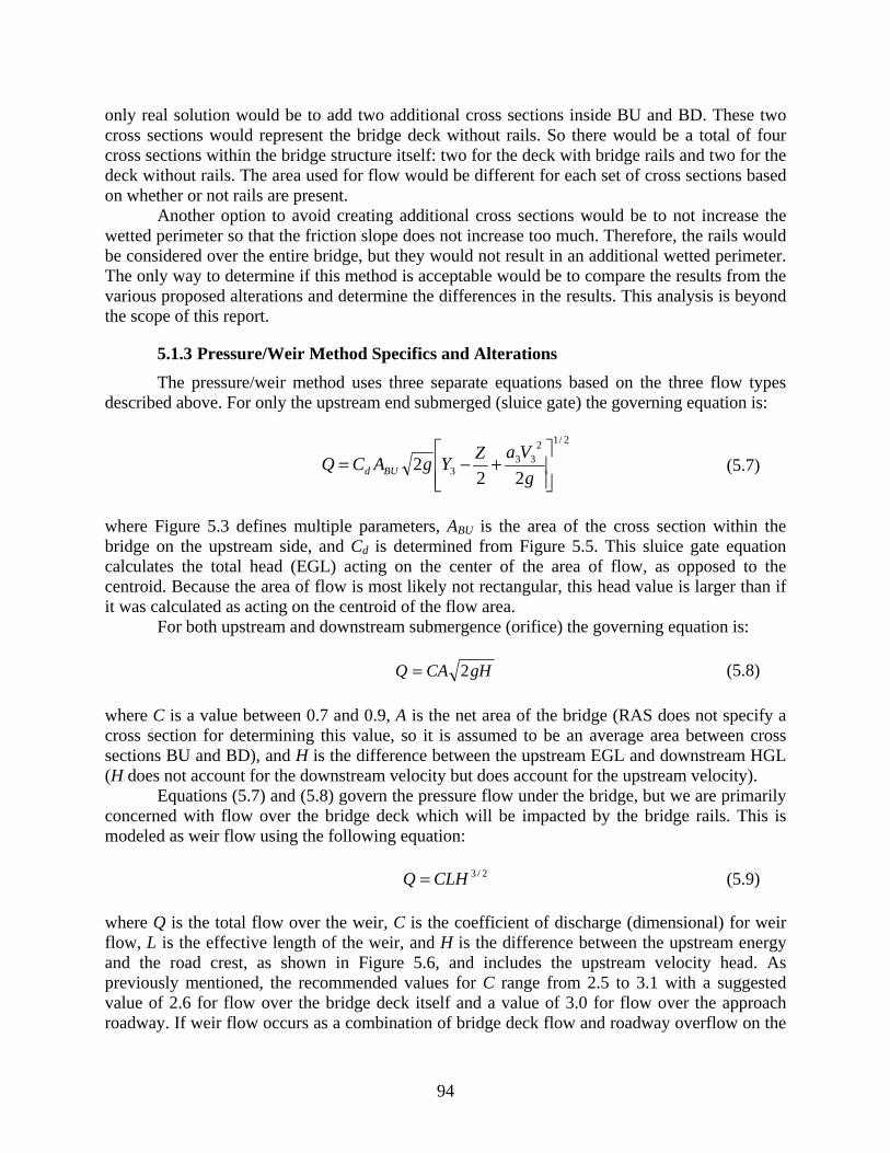
94

only real solution would be to add two additional cross sections inside BU and BD. These two cross sections would represent the bridge deck without rails. So there would be a total of four cross sections within the bridge structure itself: two for the deck with bridge rails and two for the deck without rails. The area used for flow would be different for each set of cross sections based on whether or not rails are present. Another option to avoid creating additional cross sections would be to not increase the wetted perimeter so that the friction slope does not increase too much. Therefore, the rails would be considered over the entire bridge, but they would not result in an additional wetted perimeter. The only way to determine if this method is acceptable would be to compare the results from the various proposed alterations and determine the differences in the results. This analysis is beyond the scope of this report.

5.1.3 Pressure/Weir Method Specifics and Alterations The pressure/weir method uses three separate equations based on the three flow types described above. For only the upstream end submerged (sluice gate) the governing equation is:

2/12

333 22

2⎥⎥⎦

⎤

⎢⎢⎣

⎡+−=

gVaZYgACQ BUd (5.7)

where Figure 5.3 defines multiple parameters, ABU is the area of the cross section within the bridge on the upstream side, and Cd is determined from Figure 5.5. This sluice gate equation calculates the total head (EGL) acting on the center of the area of flow, as opposed to the centroid. Because the area of flow is most likely not rectangular, this head value is larger than if it was calculated as acting on the centroid of the flow area. For both upstream and downstream submergence (orifice) the governing equation is: gHCAQ 2= (5.8) where C is a value between 0.7 and 0.9, A is the net area of the bridge (RAS does not specify a cross section for determining this value, so it is assumed to be an average area between cross sections BU and BD), and H is the difference between the upstream EGL and downstream HGL (H does not account for the downstream velocity but does account for the upstream velocity). Equations (5.7) and (5.8) govern the pressure flow under the bridge, but we are primarily concerned with flow over the bridge deck which will be impacted by the bridge rails. This is modeled as weir flow using the following equation: 2/3CLHQ = (5.9) where Q is the total flow over the weir, C is the coefficient of discharge (dimensional) for weir flow, L is the effective length of the weir, and H is the difference between the upstream energy and the road crest, as shown in Figure 5.6, and includes the upstream velocity head. As previously mentioned, the recommended values for C range from 2.5 to 3.1 with a suggested value of 2.6 for flow over the bridge deck itself and a value of 3.0 for flow over the approach roadway. If weir flow occurs as a combination of bridge deck flow and roadway overflow on the

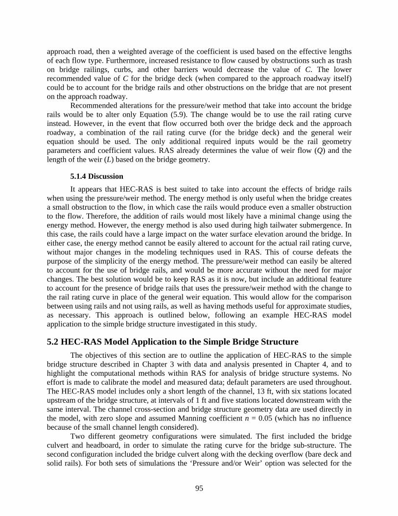
95

approach road, then a weighted average of the coefficient is used based on the effective lengths of each flow type. Furthermore, increased resistance to flow caused by obstructions such as trash on bridge railings, curbs, and other barriers would decrease the value of C. The lower recommended value of C for the bridge deck (when compared to the approach roadway itself) could be to account for the bridge rails and other obstructions on the bridge that are not present on the approach roadway. Recommended alterations for the pressure/weir method that take into account the bridge rails would be to alter only Equation (5.9). The change would be to use the rail rating curve instead. However, in the event that flow occurred both over the bridge deck and the approach roadway, a combination of the rail rating curve (for the bridge deck) and the general weir equation should be used. The only additional required inputs would be the rail geometry parameters and coefficient values. RAS already determines the value of weir flow (Q) and the length of the weir (L) based on the bridge geometry.

5.1.4 Discussion

It appears that HEC-RAS is best suited to take into account the effects of bridge rails when using the pressure/weir method. The energy method is only useful when the bridge creates a small obstruction to the flow, in which case the rails would produce even a smaller obstruction to the flow. Therefore, the addition of rails would most likely have a minimal change using the energy method. However, the energy method is also used during high tailwater submergence. In this case, the rails could have a large impact on the water surface elevation around the bridge. In either case, the energy method cannot be easily altered to account for the actual rail rating curve, without major changes in the modeling techniques used in RAS. This of course defeats the purpose of the simplicity of the energy method. The pressure/weir method can easily be altered to account for the use of bridge rails, and would be more accurate without the need for major changes. The best solution would be to keep RAS as it is now, but include an additional feature to account for the presence of bridge rails that uses the pressure/weir method with the change to the rail rating curve in place of the general weir equation. This would allow for the comparison between using rails and not using rails, as well as having methods useful for approximate studies, as necessary. This approach is outlined below, following an example HEC-RAS model application to the simple bridge structure investigated in this study.

5.2 HEC-RAS Model Application to the Simple Bridge Structure The objectives of this section are to outline the application of HEC-RAS to the simple bridge structure described in Chapter 3 with data and analysis presented in Chapter 4, and to highlight the computational methods within RAS for analysis of bridge structure systems. No effort is made to calibrate the model and measured data; default parameters are used throughout. The HEC-RAS model includes only a short length of the channel, 13 ft, with six stations located upstream of the bridge structure, at intervals of 1 ft and five stations located downstream with the same interval. The channel cross-section and bridge structure geometry data are used directly in the model, with zero slope and assumed Manning coefficient n = 0.05 (which has no influence because of the small channel length considered). Two different geometry configurations were simulated. The first included the bridge culvert and headboard, in order to simulate the rating curve for the bridge sub-structure. The second configuration included the bridge culvert along with the decking overflow (bare deck and solid rails). For both sets of simulations the ‘Pressure and/or Weir’ option was selected for the

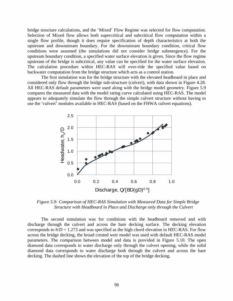
96

bridge structure calculations, and the ‘Mixed’ Flow Regime was selected for flow computation. Selection of Mixed flow allows both supercritical and subcritical flow computation within a single flow profile, though it does require specification of depth characteristics at both the upstream and downstream boundary. For the downstream boundary condition, critical flow conditions were assumed (the simulations did not consider bridge submergence). For the upstream boundary condition, a specified water surface elevation is given. Since the flow regime upstream of the bridge is subcritical, any value can be specified for the water surface elevation. The calculation procedure within HEC-RAS will over-ride the specified value based on backwater computation from the bridge structure which acts as a control station. The first simulation was for the bridge structure with the elevated headboard in place and considered only flow through the bridge sub-structure (culvert), with data shown in Figure 4.28. All HEC-RAS default parameters were used along with the bridge model geometry. Figure 5.9 compares the measured data with the model rating curve calculated using HEC-RAS. The model appears to adequately simulate the flow through the simple culvert structure without having to use the ‘culvert’ modules available in HEC-RAS (based on the FHWA culvert equations).

Figure 5.9: Comparison of HEC-RAS Simulation with Measured Data for Simple Bridge

Structure with Headboard in Place and Discharge only through the Culvert

The second simulation was for conditions with the headboard removed and with discharge through the culvert and across the bare decking surface. The decking elevation corresponds to h/D = 1.273 and was specified as the high chord elevation in HEC-RAS. For flow across the bridge decking, the broad crested weir model was used with default HEC-RAS model parameters. The comparison between model and data is provided in Figure 5.10. The open diamond data corresponds to water discharge only through the culvert opening, while the solid diamond data corresponds to water discharge both through the culvert and across the bare decking. The dashed line shows the elevation of the top of the bridge decking.

0.0

0.5

1.0

1.5

2.0

2.5

0.0 0.2 0.4 0.6 0.8 1.0

Hea

dwat

er, h

u/D

Discharge, Q/[BD(gD)0.5]

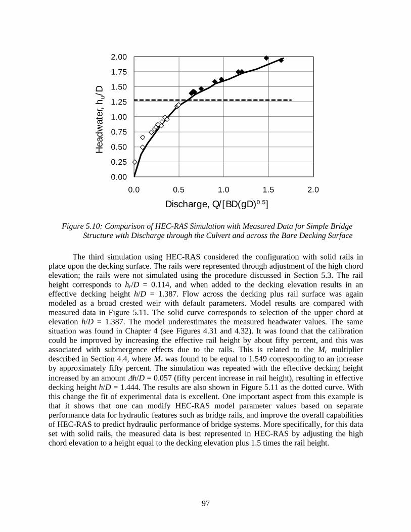
97


Structure with Discharge through the Culvert and across the Bare Decking Surface

The third simulation using HEC-RAS considered the configuration with solid rails in place upon the decking surface. The rails were represented through adjustment of the high chord elevation; the rails were not simulated using the procedure discussed in Section 5.3. The rail height corresponds to hr/D = 0.114, and when added to the decking elevation results in an effective decking height h/D = 1.387. Flow across the decking plus rail surface was again modeled as a broad crested weir with default parameters. Model results are compared with measured data in Figure 5.11. The solid curve corresponds to selection of the upper chord at elevation h/D = 1.387. The model underestimates the measured headwater values. The same situation was found in Chapter 4 (see Figures 4.31 and 4.32). It was found that the calibration could be improved by increasing the effective rail height by about fifty percent, and this was associated with submergence effects due to the rails. This is related to the Mr multiplier described in Section 4.4, where Mr was found to be equal to 1.549 corresponding to an increase by approximately fifty percent. The simulation was repeated with the effective decking height increased by an amount Δh/D = 0.057 (fifty percent increase in rail height), resulting in effective decking height h/D = 1.444. The results are also shown in Figure 5.11 as the dotted curve. With this change the fit of experimental data is excellent. One important aspect from this example is that it shows that one can modify HEC-RAS model parameter values based on separate performance data for hydraulic features such as bridge rails, and improve the overall capabilities of HEC-RAS to predict hydraulic performance of bridge systems. More specifically, for this data set with solid rails, the measured data is best represented in HEC-RAS by adjusting the high chord elevation to a height equal to the decking elevation plus 1.5 times the rail height.

0.00

0.25

0.50

0.75

1.00

1.25

1.50

1.75

2.00

0.0 0.5 1.0 1.5 2.0

Hea

dwat

er, h

u/D


98


Structure with Discharge through the Culvert and across the Decking Surface with Solid Rail

(dotted curve corresponds to increased effective rail height based on data presented in Figure 4.31)

The overall conclusion from this modeling exercise is that HEC-RAS is able to simulate measured performance data for a simple bridge structure, and that model parameters can be adjusted based on separate data to allow improved simulation of structure hydraulic performance.

5.3 Weir Coefficient Determination for Use in HEC-RAS Based on Unit Discharge One possible method of incorporating the bridge rail rating curves into HEC-RAS is to use the pressure and weir method for high flows over a bridge structure and alter the weir coefficient for a given rail type and flow conditions. For this method of calculation, the weir coefficient given in the bridge deck/roadway data editor is used to calculate the water depth above the bridge structure for a given flow rate using the following equation. 2/3CLHQ = (5.10) where Q is the total flow over the weir, C is the (dimensional) coefficient of discharge for weir flow, L is the effective length of the weir, and H is the difference between the upstream energy and the road crest, as shown in Figure 5.6, and includes the upstream velocity head. The recommended values for C range from 2.5 to 3.1 with a suggested value of 2.6 for flow over the bridge deck.

0.00

0.25

0.50

0.75

1.00

1.25

1.50

1.75

2.00

0.0 0.5 1.0 1.5

Hea

dwat

er, h

u/D


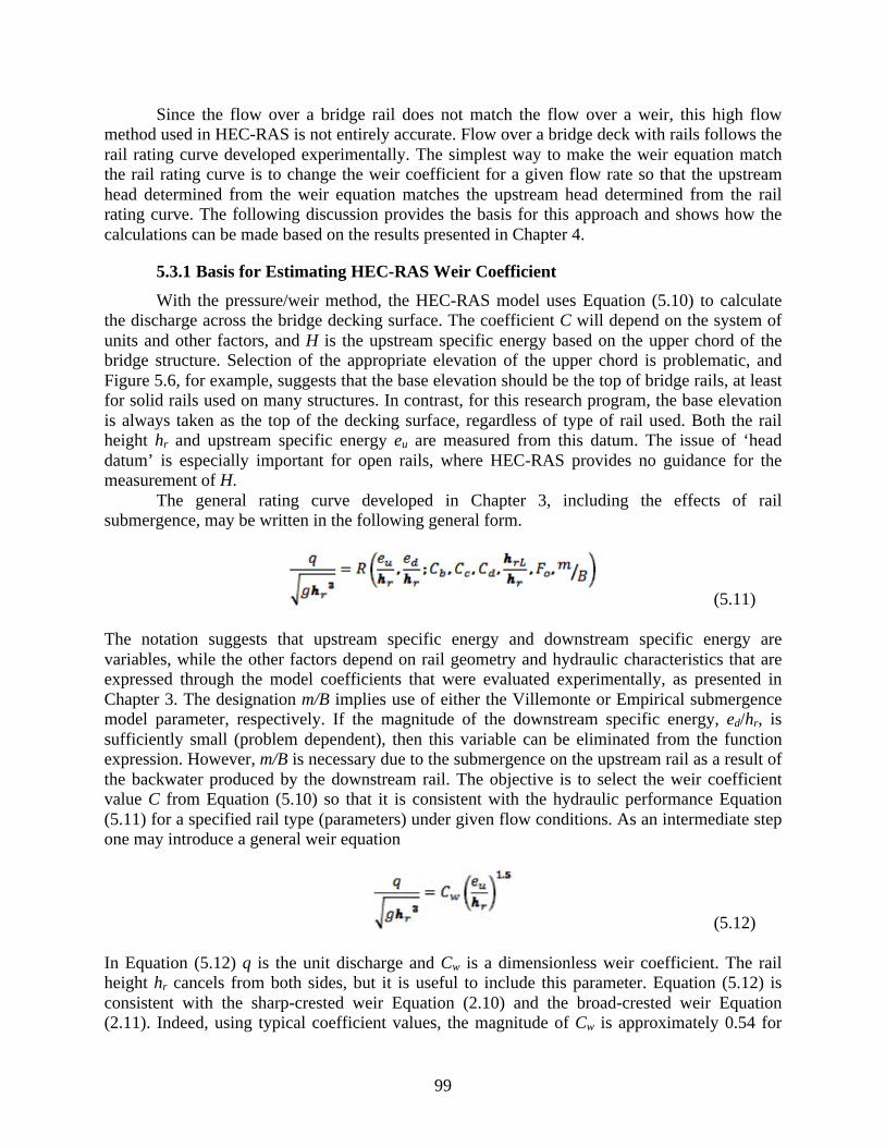
99

Since the flow over a bridge rail does not match the flow over a weir, this high flow

method used in HEC-RAS is not entirely accurate. Flow over a bridge deck with rails follows the

rail rating curve developed experimentally. The simplest way to make the weir equation match

the rail rating curve is to change the weir coefficient for a given flow rate so that the upstream

head determined from the weir equation matches the upstream head determined from the rail

rating curve. The following discussion provides the basis for this approach and shows how the

calculations can be made based on the results presented in Chapter 4.

5.3.1 Basis for Estimating HEC-RAS Weir Coefficient

With the pressure/weir method, the HEC-RAS model uses Equation (5.10) to calculate

the discharge across the bridge decking surface. The coefficient C will depend on the system of

units and other factors, and H is the upstream specific energy based on the upper chord of the

bridge structure. Selection of the appropriate elevation of the upper chord is problematic, and

Figure 5.6, for example, suggests that the base elevation should be the top of bridge rails, at least

for solid rails used on many structures. In contrast, for this research program, the base elevation

is always taken as the top of the decking surface, regardless of type of rail used. Both the rail

height hr and upstream specific energy eu are measured from this datum. The issue of ‘head

datum’ is especially important for open rails, where HEC-RAS provides no guidance for the

measurement of H.

The general rating curve developed in Chapter 3, including the effects of rail

submergence, may be written in the following general form.

(5.11)

The notation suggests that upstream specific energy and downstream specific energy are

variables, while the other factors depend on rail geometry and hydraulic characteristics that are

expressed through the model coefficients that were evaluated experimentally, as presented in

Chapter 3. The designation m/B implies use of either the Villemonte or Empirical submergence

model parameter, respectively. If the magnitude of the downstream specific energy, ed/hr, is

sufficiently small (problem dependent), then this variable can be eliminated from the function

expression. However, m/B is necessary due to the submergence on the upstream rail as a result of

the backwater produced by the downstream rail. The objective is to select the weir coefficient

value C from Equation (5.10) so that it is consistent with the hydraulic performance Equation

(5.11) for a specified rail type (parameters) under given flow conditions. As an intermediate step

one may introduce a general weir equation

(5.12)

In Equation (5.12) q is the unit discharge and Cw is a dimensionless weir coefficient. The rail

height hr cancels from both sides, but it is useful to include this parameter. Equation (5.12) is

consistent with the sharp-crested weir Equation (2.10) and the broad-crested weir Equation

(2.11). Indeed, using typical coefficient values, the magnitude of Cw is approximately 0.54 for

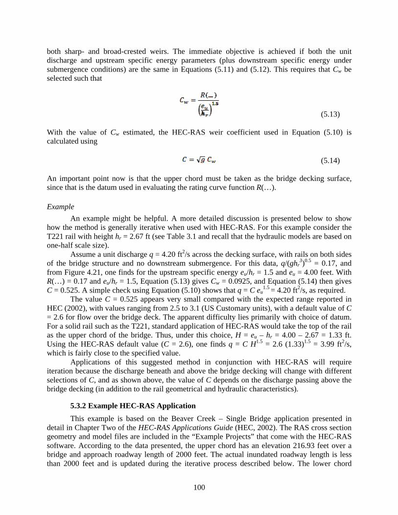
100

both sharp- and broad-crested weirs. The immediate objective is achieved if both the unit

discharge and upstream specific energy parameters (plus downstream specific energy under

submergence conditions) are the same in Equations (5.11) and (5.12). This requires that Cw be

selected such that

(5.13)

With the value of Cw estimated, the HEC-RAS weir coefficient used in Equation (5.10) is

calculated using

(5.14)

An important point now is that the upper chord must be taken as the bridge decking surface,

since that is the datum used in evaluating the rating curve function R(…).

Example

An example might be helpful. A more detailed discussion is presented below to show

how the method is generally iterative when used with HEC-RAS. For this example consider the

T221 rail with height hr = 2.67 ft (see Table 3.1 and recall that the hydraulic models are based on

one-half scale size).

Assume a unit discharge q = 4.20 ft2/s across the decking surface, with rails on both sides

of the bridge structure and no downstream submergence. For this data, q/(ghr3)

0.5 = 0.17, and

from Figure 4.21, one finds for the upstream specific energy eu/hr = 1.5 and eu = 4.00 feet. With

R(…) = 0.17 and eu/hr = 1.5, Equation (5.13) gives Cw = 0.0925, and Equation (5.14) then gives

C = 0.525. A simple check using Equation (5.10) shows that q = C eu1.5

= 4.20 ft2/s, as required.

The value C = 0.525 appears very small compared with the expected range reported in

HEC (2002), with values ranging from 2.5 to 3.1 (US Customary units), with a default value of C

= 2.6 for flow over the bridge deck. The apparent difficulty lies primarily with choice of datum.

For a solid rail such as the T221, standard application of HEC-RAS would take the top of the rail

as the upper chord of the bridge. Thus, under this choice, H = eu – hr = 4.00 – 2.67 = 1.33 ft.

Using the HEC-RAS default value (C = 2.6), one finds q = C H1.5

= 2.6 (1.33)1.5

= 3.99 ft2/s,

which is fairly close to the specified value.

Applications of this suggested method in conjunction with HEC-RAS will require

iteration because the discharge beneath and above the bridge decking will change with different

selections of C, and as shown above, the value of C depends on the discharge passing above the

bridge decking (in addition to the rail geometrical and hydraulic characteristics).

5.3.2 Example HEC-RAS Application

This example is based on the Beaver Creek – Single Bridge application presented in

detail in Chapter Two of the HEC-RAS Applications Guide (HEC, 2002). The RAS cross section

geometry and model files are included in the “Example Projects” that come with the HEC-RAS

software. According to the data presented, the upper chord has an elevation 216.93 feet over a

bridge and approach roadway length of 2000 feet. The actual inundated roadway length is less

than 2000 feet and is updated during the iterative process described below. The lower chord

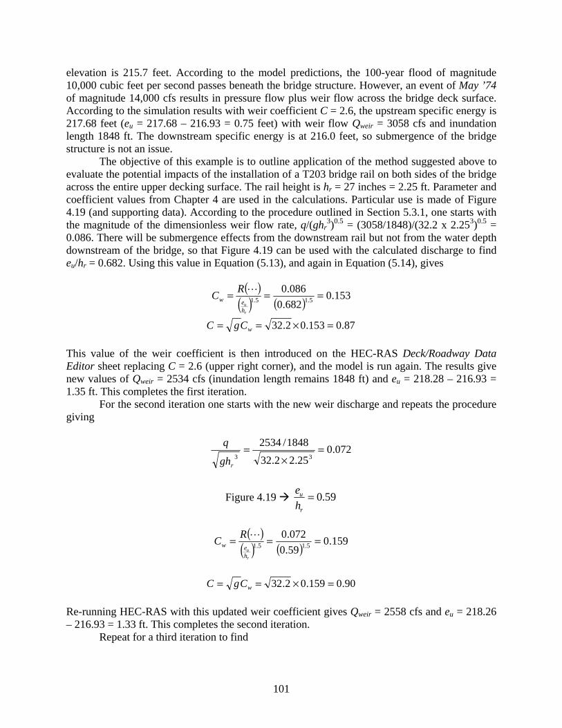
101

elevation is 215.7 feet. According to the model predictions, the 100-year flood of magnitude 10,000 cubic feet per second passes beneath the bridge structure. However, an event of May ’74 of magnitude 14,000 cfs results in pressure flow plus weir flow across the bridge deck surface. According to the simulation results with weir coefficient C = 2.6, the upstream specific energy is 217.68 feet (eu = 217.68 – 216.93 = 0.75 feet) with weir flow Qweir = 3058 cfs and inundation length 1848 ft. The downstream specific energy is at 216.0 feet, so submergence of the bridge structure is not an issue. The objective of this example is to outline application of the method suggested above to evaluate the potential impacts of the installation of a T203 bridge rail on both sides of the bridge across the entire upper decking surface. The rail height is hr = 27 inches = 2.25 ft. Parameter and coefficient values from Chapter 4 are used in the calculations. Particular use is made of Figure 4.19 (and supporting data). According to the procedure outlined in Section 5.3.1, one starts with the magnitude of the dimensionless weir flow rate, q/(ghr

3)0.5 = (3058/1848)/(32.2 x 2.253)0.5 = 0.086. There will be submergence effects from the downstream rail but not from the water depth downstream of the bridge, so that Figure 4.19 can be used with the calculated discharge to find eu/hr = 0.682. Using this value in Equation (5.13), and again in Equation (5.14), gives

( )( ) ( ) 153.0

682.0086.0

5.15.1 ===r

uhew

RC L

87.0153.02.32 =×== wCgC This value of the weir coefficient is then introduced on the HEC-RAS Deck/Roadway Data Editor sheet replacing C = 2.6 (upper right corner), and the model is run again. The results give new values of Qweir = 2534 cfs (inundation length remains 1848 ft) and eu = 218.28 – 216.93 = 1.35 ft. This completes the first iteration. For the second iteration one starts with the new weir discharge and repeats the procedure giving

072.025.22.32

1848/253433

=×

=rgh

q

Figure 4.19 59.0=r

u

he

( )

( ) ( ) 159.059.0072.0

5.15.1 ===r

uhew

RC L

90.0159.02.32 =×== wCgC Re-running HEC-RAS with this updated weir coefficient gives Qweir = 2558 cfs and eu = 218.26 – 216.93 = 1.33 ft. This completes the second iteration. Repeat for a third iteration to find

102

072.025.22.32

1848/255833

=×

=rgh

q

For the two significant figures, this is the same as found from the second iteration so the iterative method has converged (use of more significant figures will result in more iterations to achieve convergence, but the procedure does not change). The results from this example suggest that installation of T203 rails on the bridge and roadway would result in an increase in the upstream headwater by 0.58 feet (from 0.75 feet to 1.33 feet on the bridge deck surface) and a decrease in the flow across the bridge decking by approximately 500 cfs (from 3058 cfs to 2558 cfs) for this storm event.

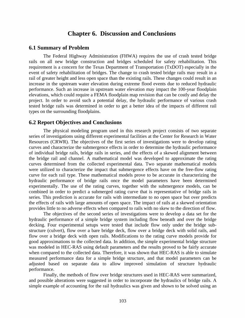
103

Chapter 6. Discussion and Conclusions

6.1 Summary of Problem The Federal Highway Administration (FHWA) requires the use of crash tested bridge rails on all new bridge construction and bridges scheduled for safety rehabilitation. This requirement is a concern for the Texas Department of Transportation (TxDOT) especially in the event of safety rehabilitation of bridges. The change to crash tested bridge rails may result in a rail of greater height and less open space than the existing rails. These changes could result in an increase in the upstream water elevation during extreme flood events due to reduced hydraulic performance. Such an increase in upstream water elevation may impact the 100-year floodplain elevations, which could require a FEMA floodplain map revision that can be costly and delay the project. In order to avoid such a potential delay, the hydraulic performance of various crash tested bridge rails was determined in order to get a better idea of the impacts of different rail types on the surrounding floodplains.

6.2 Report Objectives and Conclusions The physical modeling program used in this research project consists of two separate

series of investigations using different experimental facilities at the Center for Research in Water Resources (CRWR). The objectives of the first series of investigations were to develop rating curves and characterize the submergence effects in order to determine the hydraulic performance of individual bridge rails, bridge rails in series, and the effects of a skewed alignment between the bridge rail and channel. A mathematical model was developed to approximate the rating curves determined from the collected experimental data. Two separate mathematical models were utilized to characterize the impact that submergence effects have on the free-flow rating curve for each rail type. These mathematical models prove to be accurate in characterizing the hydraulic performance of bridge rails once the model parameters have been determined experimentally. The use of the rating curves, together with the submergence models, can be combined in order to predict a submerged rating curve that is representative of bridge rails in series. This prediction is accurate for rails with intermediate to no open space but over predicts the effects of rails with large amounts of open space. The impact of rails at a skewed orientation provides little to no adverse effects when compared to rails with no skew to the direction of flow.

The objectives of the second series of investigations were to develop a data set for the hydraulic performance of a simple bridge system including flow beneath and over the bridge decking. Four experimental setups were tested that include flow only under the bridge sub-structure (culvert), flow over a bare bridge deck, flow over a bridge deck with solid rails, and flow over a bridge deck with open rails. Modifications to the rating curve models provide for good approximations to the collected data. In addition, the simple experimental bridge structure was modeled in HEC-RAS using default parameters and the results proved to be fairly accurate when compared to the collected data. Therefore, it was shown that HEC-RAS is able to simulate measured performance data for a simple bridge structure, and that model parameters can be adjusted based on separate data to allow improved simulation of structure hydraulic performance.

Finally, the methods of flow over bridge structures used in HEC-RAS were summarized, and possible alterations were suggested in order to incorporate the hydraulics of bridge rails. A simple example of accounting for the rail hydraulics was given and shown to be solved using an

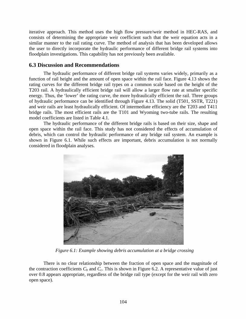
104

iterative approach. This method uses the high flow pressure/weir method in HEC-RAS, and consists of determining the appropriate weir coefficient such that the weir equation acts in a similar manner to the rail rating curve. The method of analysis that has been developed allows the user to directly incorporate the hydraulic performance of different bridge rail systems into floodplain investigations. This capability has not previously been available.

6.3 Discussion and Recommendations The hydraulic performance of different bridge rail systems varies widely, primarily as a function of rail height and the amount of open space within the rail face. Figure 4.13 shows the rating curves for the different bridge rail types on a common scale based on the height of the T203 rail. A hydraulically efficient bridge rail will allow a larger flow rate at smaller specific energy. Thus, the ‘lower’ the rating curve, the more hydraulically efficient the rail. Three groups of hydraulic performance can be identified through Figure 4.13. The solid (T501, SSTR, T221) and weir rails are least hydraulically efficient. Of intermediate efficiency are the T203 and T411 bridge rails. The most efficient rails are the T101 and Wyoming two-tube rails. The resulting model coefficients are listed in Table 4.1. The hydraulic performance of the different bridge rails is based on their size, shape and open space within the rail face. This study has not considered the effects of accumulation of debris, which can control the hydraulic performance of any bridge rail system. An example is shown in Figure 6.1. While such effects are important, debris accumulation is not normally considered in floodplain analyses.

Figure 6.1: Example showing debris accumulation at a bridge crossing

There is no clear relationship between the fraction of open space and the magnitude of the contraction coefficients Cb and Cc. This is shown in Figure 6.2. A representative value of just over 0.8 appears appropriate, regardless of the bridge rail type (except for the weir rail with zero open space).

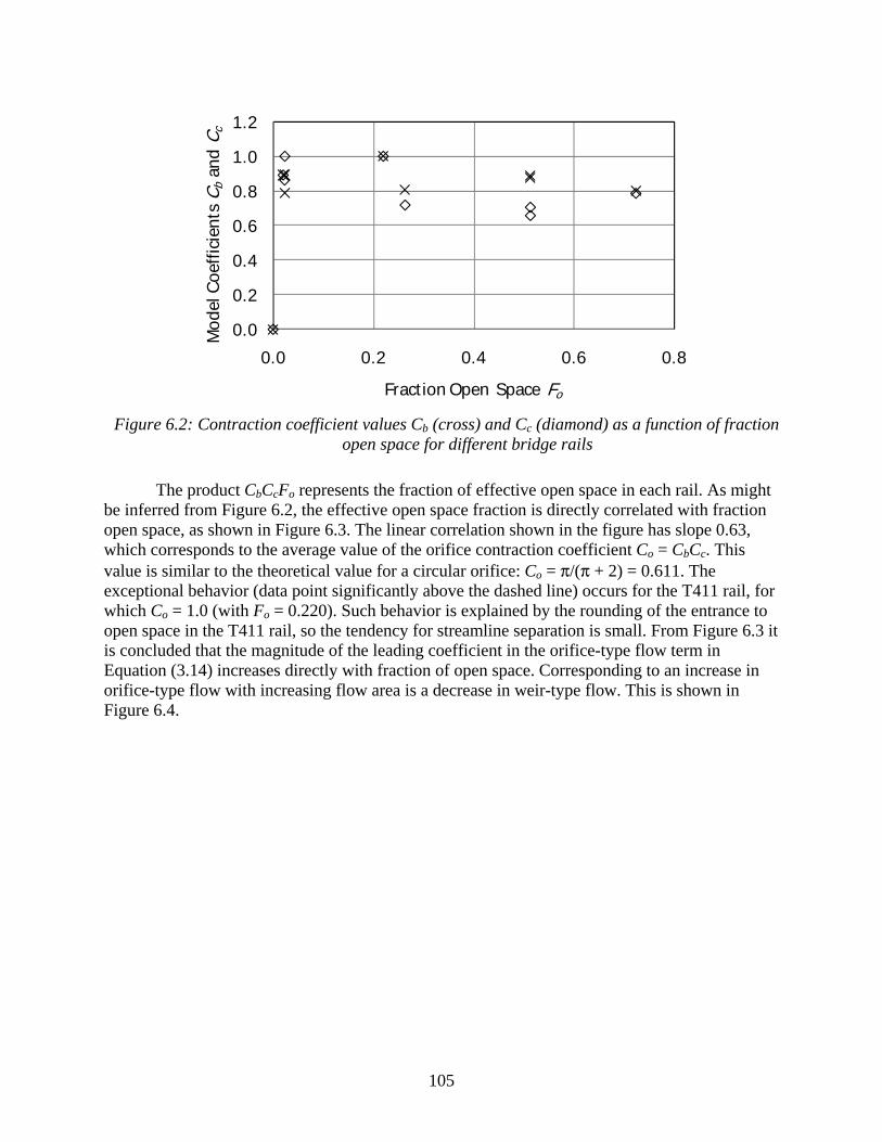
105

Figure 6.2: Contraction coefficient values Cb (cross) and Cc (diamond) as a function of fraction

open space for different bridge rails

The product CbCcFo represents the fraction of effective open space in each rail. As might be inferred from Figure 6.2, the effective open space fraction is directly correlated with fraction open space, as shown in Figure 6.3. The linear correlation shown in the figure has slope 0.63, which corresponds to the average value of the orifice contraction coefficient Co = CbCc. This value is similar to the theoretical value for a circular orifice: Co = π/(π + 2) = 0.611. The exceptional behavior (data point significantly above the dashed line) occurs for the T411 rail, for which Co = 1.0 (with Fo = 0.220). Such behavior is explained by the rounding of the entrance to open space in the T411 rail, so the tendency for streamline separation is small. From Figure 6.3 it is concluded that the magnitude of the leading coefficient in the orifice-type flow term in Equation (3.14) increases directly with fraction of open space. Corresponding to an increase in orifice-type flow with increasing flow area is a decrease in weir-type flow. This is shown in Figure 6.4.

0.0

0.2

0.4

0.6

0.8

1.0

1.2

0.0 0.2 0.4 0.6 0.8

Mod

el C

oeffic

ient

s C b

and

C c

Fraction Open Space Fo

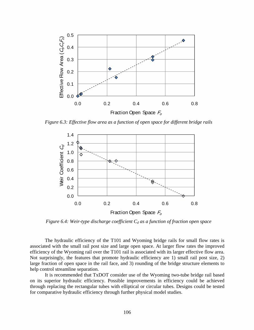
106

Figure 6.3: Effective flow area as a function of open space for different bridge rails

Figure 6.4: Weir-type discharge coefficient Cd as a function of fraction open space

The hydraulic efficiency of the T101 and Wyoming bridge rails for small flow rates is

associated with the small rail post size and large open space. At larger flow rates the improved efficiency of the Wyoming rail over the T101 rail is associated with its larger effective flow area. Not surprisingly, the features that promote hydraulic efficiency are 1) small rail post size, 2) large fraction of open space in the rail face, and 3) rounding of the bridge structure elements to help control streamline separation.

It is recommended that TxDOT consider use of the Wyoming two-tube bridge rail based on its superior hydraulic efficiency. Possible improvements in efficiency could be achieved through replacing the rectangular tubes with elliptical or circular tubes. Designs could be tested for comparative hydraulic efficiency through further physical model studies.

0.0

0.1

0.2

0.3

0.4

0.5

0.0 0.2 0.4 0.6 0.8

Effe

ctiv

e Fl

ow A

rea

(CbC

cFo)


0.0

0.2

0.4

0.6

0.8

1.0

1.2

1.4

0.0 0.2 0.4 0.6 0.8

Wei

r Coe

ffic

ient

Cd


107

References

Benson, K.S. (2004): Hydraulic Effects of Safety End Treatments on Culvert Performance, M.S. Thesis in Engineering, The University of Texas at Austin.

Bos, M.G. (1989): Discharge Measurement Structures, Publication 20, Third revised edition, International Institute for Land Reclamation and Improvement, Wageningen, The Netherlands.

Bradley, J.N. (1978): Hydraulics of Bridge Waterways, Hydraulics Design Series 1, Federal Highway Administration, Washington D.C.

Charbeneau, R.J., Henderson, A.D., and Sherman, L.C. (2006): “Hydraulic Performance Curves for Highway Culverts,” Journal of Hydraulic Engineering, Vol. 132, No. 5, p. 474-481.

Charbeneau, R.J. and Holley, E.R. (2001): Backwater Effects of Piers in Subcritical Flow, Research Report, Report No. FHWA/TX-0-1805-1, Center for Transportation Research, Bureau of Engineering Research, Austin, TX.

Chow, V.T. (1959): Open-Channel Hydraulics, McGraw-Hill, New York.

FHWA (2005): Bridge Rail Guide 2005, Federal Highway Administration, California Division.

FHWA (2007): FHWA Caltrans Bridge Rail Guide 2005, 25 September 2007, U.S. Department of Transportation, Federal Highway Administration, <http://www.fhwa.dot.gov/bridge/bridgerail>

Hamill, Les (1999): Bridge Hydraulics, E & FN Spon, New York.

HEC (1995): RD-42, Flow Transitions in Bridgewater Analysis, Hydrologic Engineering Center, U.S. Army Corps of Engineers, Davis, CA.

HEC (2002): CPD-69, HEC-RAS, River Analysis System Hydraulic Reference Guide, Version 3.1, Hydrologic Engineering Center, U.S. Army Corps of Engineers, Davis, CA.

HEC (2002): CPD-70, HEC-RAS, River Analysis System Applications Guide, Version 3.1, Hydrologic Engineering Center, U.S. Army Corps of Engineers, Davis, CA.

Henderson, F.M. (1966): Open Channel Flow, Macmillan Publishing Co., Inc., New York.

King, H.W. and Brater, E.F. (1963): Handbook of Hydraulics, Fifth edition, McGraw-Hill Book Company, New York.

Ross, H.E., Sicking, D.L., Zimmer, R.A., and Michie, J.D. (1993): National Cooperative Highway Research Program Report 350: Recommended Procedures for the Safety Performance Evaluation of Highway Features, Transportation Research Board, National Research Council, National Academy Press, Washington, D.C.

108

Rouse, Hunter (1950): Engineering Hydraulics, Proceedings of the Fourth Hydraulics Conference, Iowa Institute of Hydraulic Research, June 12-15, 1949, John Wiley & Sons, Inc., New York.

TxDOT (2004): Hydraulic Design Manual, Texas Department of Transportation, Austin, TX.

TxDOT (2005): Bridge Railing Manual, Texas Department of Transportation, Austin, TX.

TxDOT (2007): Bridge Standards, 15 March 2007, Texas Department of Transportation, Bridge Division, <http://www.dot.state.tx.us/insdtdot/ orgchart/cmd/cserve/standard/bridge-e.htm>

Villemonte, J.R. (1947): “Submerged-Weir Discharge Studies,” Engineering News-Record, p. 866-869.

Warnock, J.E. (1950): “Hydraulic Similitude,” Engineering Hydraulics, H. Rouse (Ed.), John Wiley & Sons, Inc., New York.

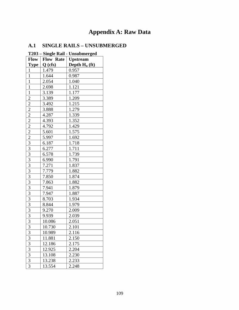
109

Appendix A: Raw Data

A.1 SINGLE RAILS – UNSUBMERGED T203 – Single Rail - Unsubmerged Flow Type

Flow Rate Q (cfs)

Upstream Depth Hu (ft)

1 1.479 0.957 1 1.644 0.987 1 2.054 1.040 1 2.698 1.121 1 3.139 1.177 2 3.389 1.209 2 3.492 1.215 2 3.888 1.279 2 4.287 1.339 2 4.393 1.352 2 4.792 1.429 2 5.601 1.575 2 5.997 1.692 3 6.187 1.718 3 6.277 1.711 3 6.578 1.739 3 6.990 1.791 3 7.271 1.837 3 7.779 1.882 3 7.850 1.874 3 7.863 1.882 3 7.941 1.879 3 7.947 1.887 3 8.703 1.934 3 8.844 1.979 3 9.270 2.009 3 9.939 2.039 3 10.086 2.051 3 10.730 2.101 3 10.989 2.116 3 11.881 2.150 3 12.186 2.175 3 12.925 2.204 3 13.108 2.230 3 13.238 2.233 3 13.554 2.248

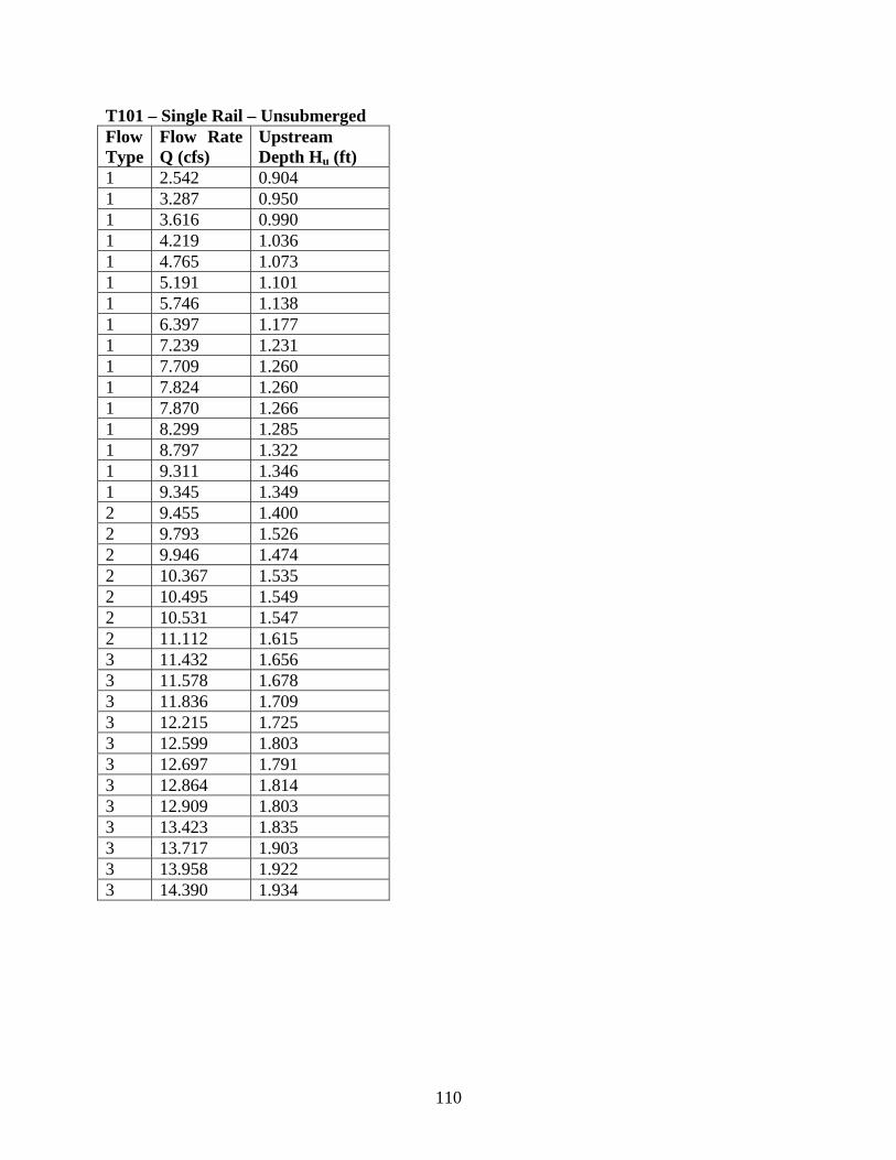
110

T101 – Single Rail – Unsubmerged Flow Type

Flow Rate Q (cfs)


1 2.542 0.904 1 3.287 0.950 1 3.616 0.990 1 4.219 1.036 1 4.765 1.073 1 5.191 1.101 1 5.746 1.138 1 6.397 1.177 1 7.239 1.231 1 7.709 1.260 1 7.824 1.260 1 7.870 1.266 1 8.299 1.285 1 8.797 1.322 1 9.311 1.346 1 9.345 1.349 2 9.455 1.400 2 9.793 1.526 2 9.946 1.474 2 10.367 1.535 2 10.495 1.549 2 10.531 1.547 2 11.112 1.615 3 11.432 1.656 3 11.578 1.678 3 11.836 1.709 3 12.215 1.725 3 12.599 1.803 3 12.697 1.791 3 12.864 1.814 3 12.909 1.803 3 13.423 1.835 3 13.717 1.903 3 13.958 1.922 3 14.390 1.934

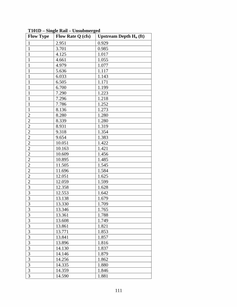
111

T101D – Single Rail – Unsubmerged Flow Type Flow Rate Q (cfs) Upstream Depth Hu (ft) 1 2.951 0.929 1 3.701 0.985 1 4.125 1.017 1 4.661 1.055 1 4.979 1.077 1 5.636 1.117 1 6.033 1.143 1 6.505 1.171 1 6.700 1.199 1 7.290 1.223 1 7.296 1.218 1 7.786 1.252 1 8.136 1.273 2 8.280 1.280 2 8.339 1.280 2 8.931 1.319 2 9.318 1.354 2 9.654 1.383 2 10.051 1.422 2 10.163 1.421 2 10.609 1.456 2 10.895 1.485 2 11.505 1.545 2 11.696 1.584 2 12.051 1.625 2 12.059 1.599 3 12.358 1.628 3 12.553 1.642 3 13.138 1.679 3 13.330 1.709 3 13.346 1.765 3 13.361 1.788 3 13.608 1.749 3 13.861 1.821 3 13.771 1.853 3 13.841 1.857 3 13.896 1.816 3 14.130 1.837 3 14.146 1.879 3 14.256 1.862 3 14.335 1.880 3 14.359 1.846 3 14.590 1.881

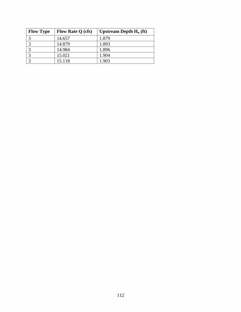
112

Flow Type Flow Rate Q (cfs) Upstream Depth Hu (ft) 3 14.657 1.879 3 14.879 1.893 3 14.984 1.896 3 15.021 1.904 3 15.118 1.903

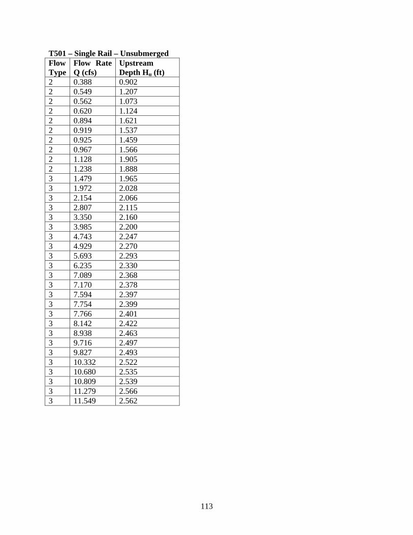
113


Flow Rate Q (cfs)


2 0.388 0.902 2 0.549 1.207 2 0.562 1.073 2 0.620 1.124 2 0.894 1.621 2 0.919 1.537 2 0.925 1.459 2 0.967 1.566 2 1.128 1.905 2 1.238 1.888 3 1.479 1.965 3 1.972 2.028 3 2.154 2.066 3 2.807 2.115 3 3.350 2.160 3 3.985 2.200 3 4.743 2.247 3 4.929 2.270 3 5.693 2.293 3 6.235 2.330 3 7.089 2.368 3 7.170 2.378 3 7.594 2.397 3 7.754 2.399 3 7.766 2.401 3 8.142 2.422 3 8.938 2.463 3 9.716 2.497 3 9.827 2.493 3 10.332 2.522 3 10.680 2.535 3 10.809 2.539 3 11.279 2.566 3 11.549 2.562

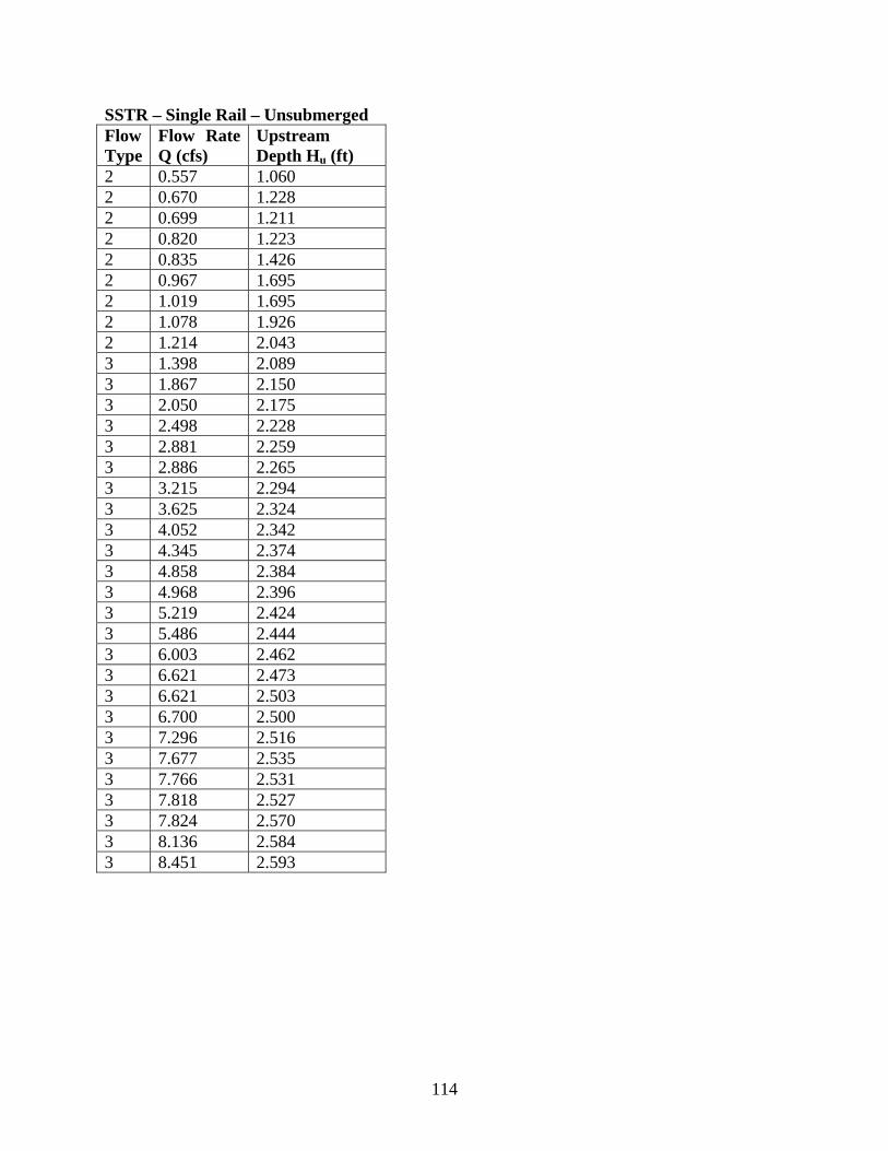
114

SSTR – Single Rail – Unsubmerged Flow Type

Flow Rate Q (cfs)


2 0.557 1.060 2 0.670 1.228 2 0.699 1.211 2 0.820 1.223 2 0.835 1.426 2 0.967 1.695 2 1.019 1.695 2 1.078 1.926 2 1.214 2.043 3 1.398 2.089 3 1.867 2.150 3 2.050 2.175 3 2.498 2.228 3 2.881 2.259 3 2.886 2.265 3 3.215 2.294 3 3.625 2.324 3 4.052 2.342 3 4.345 2.374 3 4.858 2.384 3 4.968 2.396 3 5.219 2.424 3 5.486 2.444 3 6.003 2.462 3 6.621 2.473 3 6.621 2.503 3 6.700 2.500 3 7.296 2.516 3 7.677 2.535 3 7.766 2.531 3 7.818 2.527 3 7.824 2.570 3 8.136 2.584 3 8.451 2.593

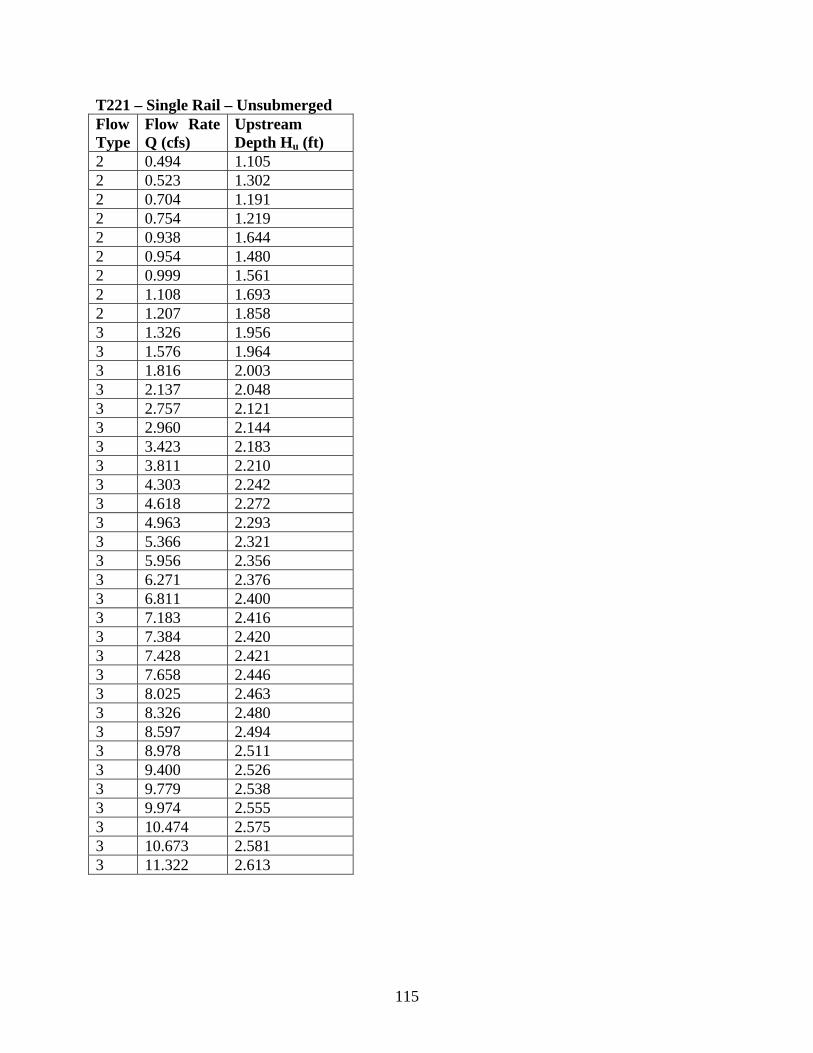
115


Flow Rate Q (cfs)


2 0.494 1.105 2 0.523 1.302 2 0.704 1.191 2 0.754 1.219 2 0.938 1.644 2 0.954 1.480 2 0.999 1.561 2 1.108 1.693 2 1.207 1.858 3 1.326 1.956 3 1.576 1.964 3 1.816 2.003 3 2.137 2.048 3 2.757 2.121 3 2.960 2.144 3 3.423 2.183 3 3.811 2.210 3 4.303 2.242 3 4.618 2.272 3 4.963 2.293 3 5.366 2.321 3 5.956 2.356 3 6.271 2.376 3 6.811 2.400 3 7.183 2.416 3 7.384 2.420 3 7.428 2.421 3 7.658 2.446 3 8.025 2.463 3 8.326 2.480 3 8.597 2.494 3 8.978 2.511 3 9.400 2.526 3 9.779 2.538 3 9.974 2.555 3 10.474 2.575 3 10.673 2.581 3 11.322 2.613

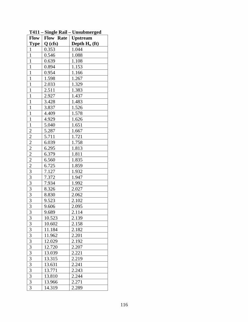
116


Flow Rate Q (cfs)


1 0.353 1.044 1 0.546 1.088 1 0.639 1.108 1 0.894 1.153 1 0.954 1.166 1 1.598 1.267 1 2.033 1.329 1 2.511 1.383 1 2.927 1.437 1 3.428 1.483 1 3.837 1.526 1 4.409 1.578 1 4.929 1.626 1 5.040 1.651 2 5.287 1.667 2 5.711 1.721 2 6.039 1.758 2 6.295 1.813 2 6.379 1.811 2 6.560 1.835 2 6.725 1.859 3 7.127 1.932 3 7.372 1.947 3 7.934 1.992 3 8.326 2.027 3 8.830 2.062 3 9.523 2.102 3 9.606 2.095 3 9.689 2.114 3 10.523 2.139 3 10.602 2.158 3 11.184 2.182 3 11.962 2.201 3 12.029 2.192 3 12.720 2.207 3 13.039 2.221 3 13.315 2.219 3 13.631 2.241 3 13.771 2.243 3 13.810 2.244 3 13.966 2.271 3 14.319 2.289

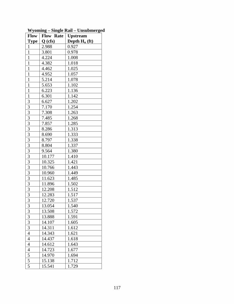
117

Wyoming – Single Rail – Unsubmerged Flow Type

Flow Rate Q (cfs)


1 2.988 0.927 1 3.801 0.978 1 4.224 1.008 1 4.382 1.018 1 4.462 1.025 1 4.952 1.057 1 5.214 1.078 1 5.653 1.102 1 6.223 1.136 1 6.301 1.142 3 6.627 1.202 3 7.170 1.254 3 7.308 1.263 3 7.485 1.268 3 7.857 1.285 3 8.286 1.313 3 8.690 1.333 3 8.797 1.338 3 8.804 1.337 3 9.564 1.380 3 10.177 1.410 3 10.325 1.421 3 10.766 1.443 3 10.960 1.449 3 11.623 1.485 3 11.896 1.502 3 12.208 1.512 3 12.283 1.517 3 12.720 1.537 3 13.054 1.540 3 13.508 1.572 3 13.888 1.591 3 14.107 1.605 3 14.311 1.612 4 14.343 1.621 4 14.437 1.618 4 14.612 1.643 4 14.723 1.677 5 14.970 1.694 5 15.138 1.712 5 15.541 1.729

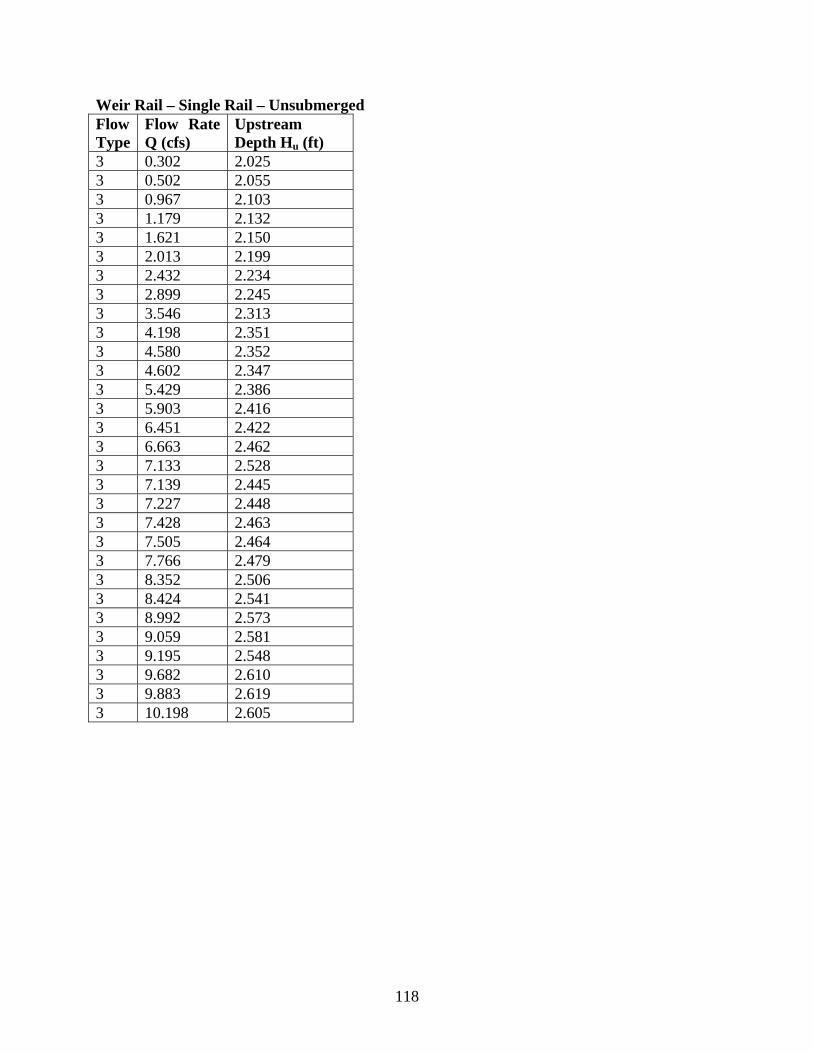
118

Weir Rail – Single Rail – Unsubmerged Flow Type

Flow Rate Q (cfs)


3 0.302 2.025 3 0.502 2.055 3 0.967 2.103 3 1.179 2.132 3 1.621 2.150 3 2.013 2.199 3 2.432 2.234 3 2.899 2.245 3 3.546 2.313 3 4.198 2.351 3 4.580 2.352 3 4.602 2.347 3 5.429 2.386 3 5.903 2.416 3 6.451 2.422 3 6.663 2.462 3 7.133 2.528 3 7.139 2.445 3 7.227 2.448 3 7.428 2.463 3 7.505 2.464 3 7.766 2.479 3 8.352 2.506 3 8.424 2.541 3 8.992 2.573 3 9.059 2.581 3 9.195 2.548 3 9.682 2.610 3 9.883 2.619 3 10.198 2.605

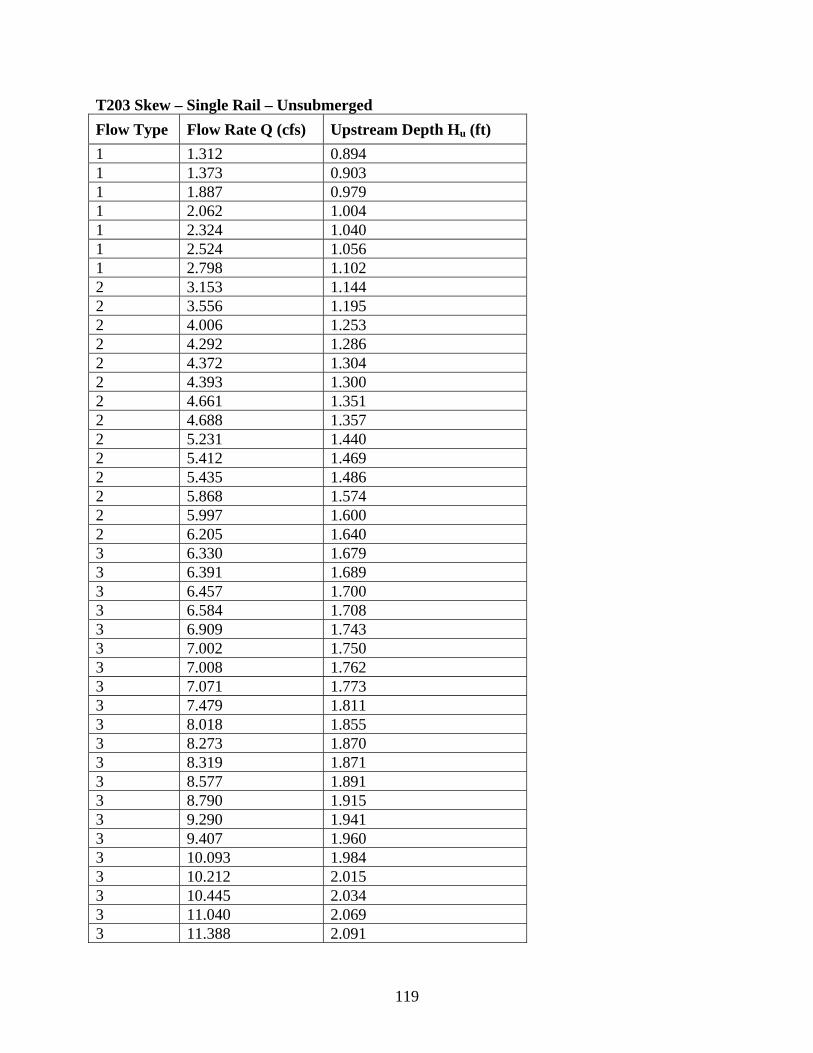
119

T203 Skew – Single Rail – Unsubmerged Flow Type Flow Rate Q (cfs) Upstream Depth Hu (ft) 1 1.312 0.894 1 1.373 0.903 1 1.887 0.979 1 2.062 1.004 1 2.324 1.040 1 2.524 1.056 1 2.798 1.102 2 3.153 1.144 2 3.556 1.195 2 4.006 1.253 2 4.292 1.286 2 4.372 1.304 2 4.393 1.300 2 4.661 1.351 2 4.688 1.357 2 5.231 1.440 2 5.412 1.469 2 5.435 1.486 2 5.868 1.574 2 5.997 1.600 2 6.205 1.640 3 6.330 1.679 3 6.391 1.689 3 6.457 1.700 3 6.584 1.708 3 6.909 1.743 3 7.002 1.750 3 7.008 1.762 3 7.071 1.773 3 7.479 1.811 3 8.018 1.855 3 8.273 1.870 3 8.319 1.871 3 8.577 1.891 3 8.790 1.915 3 9.290 1.941 3 9.407 1.960 3 10.093 1.984 3 10.212 2.015 3 10.445 2.034 3 11.040 2.069 3 11.388 2.091

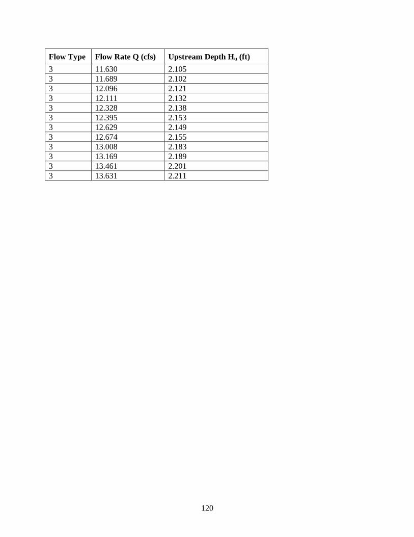
120

Flow Type Flow Rate Q (cfs) Upstream Depth Hu (ft) 3 11.630 2.105 3 11.689 2.102 3 12.096 2.121 3 12.111 2.132 3 12.328 2.138 3 12.395 2.153 3 12.629 2.149 3 12.674 2.155 3 13.008 2.183 3 13.169 2.189 3 13.461 2.201 3 13.631 2.211

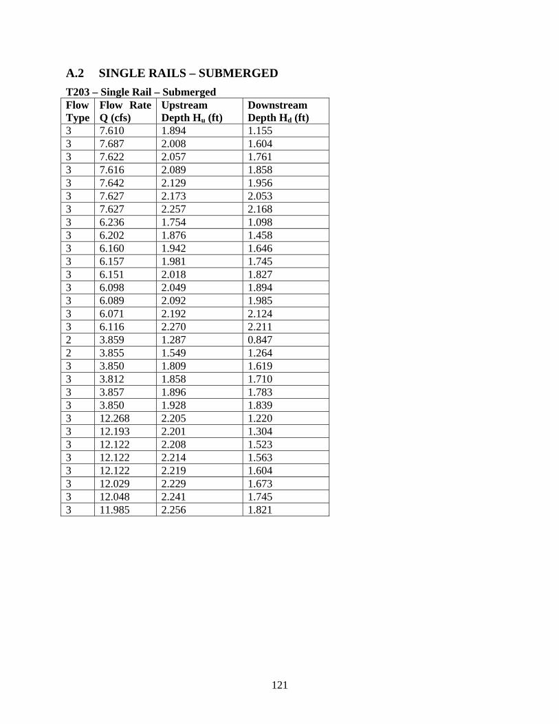
121

A.2 SINGLE RAILS – SUBMERGED T203 – Single Rail – Submerged Flow Type

Flow Rate Q (cfs)


Downstream Depth Hd (ft)

3 7.610 1.894 1.155 3 7.687 2.008 1.604 3 7.622 2.057 1.761 3 7.616 2.089 1.858 3 7.642 2.129 1.956 3 7.627 2.173 2.053 3 7.627 2.257 2.168 3 6.236 1.754 1.098 3 6.202 1.876 1.458 3 6.160 1.942 1.646 3 6.157 1.981 1.745 3 6.151 2.018 1.827 3 6.098 2.049 1.894 3 6.089 2.092 1.985 3 6.071 2.192 2.124 3 6.116 2.270 2.211 2 3.859 1.287 0.847 2 3.855 1.549 1.264 3 3.850 1.809 1.619 3 3.812 1.858 1.710 3 3.857 1.896 1.783 3 3.850 1.928 1.839 3 12.268 2.205 1.220 3 12.193 2.201 1.304 3 12.122 2.208 1.523 3 12.122 2.214 1.563 3 12.122 2.219 1.604 3 12.029 2.229 1.673 3 12.048 2.241 1.745 3 11.985 2.256 1.821

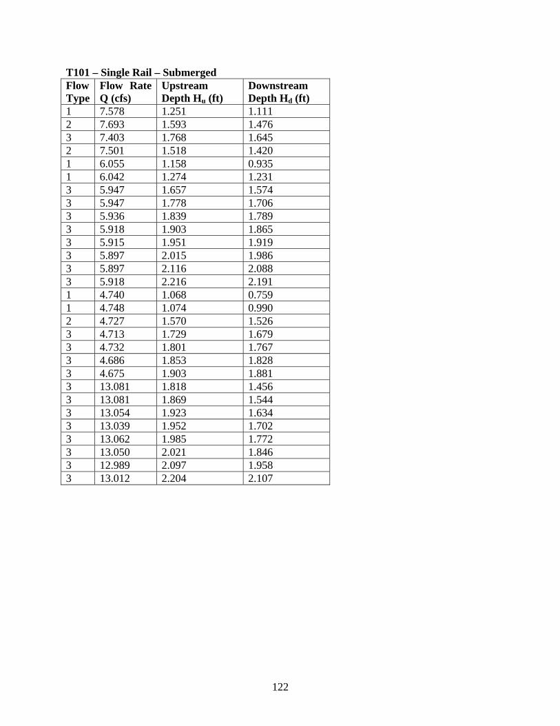
122

T101 – Single Rail – Submerged Flow Type

Flow Rate Q (cfs)



1 7.578 1.251 1.111 2 7.693 1.593 1.476 3 7.403 1.768 1.645 2 7.501 1.518 1.420 1 6.055 1.158 0.935 1 6.042 1.274 1.231 3 5.947 1.657 1.574 3 5.947 1.778 1.706 3 5.936 1.839 1.789 3 5.918 1.903 1.865 3 5.915 1.951 1.919 3 5.897 2.015 1.986 3 5.897 2.116 2.088 3 5.918 2.216 2.191 1 4.740 1.068 0.759 1 4.748 1.074 0.990 2 4.727 1.570 1.526 3 4.713 1.729 1.679 3 4.732 1.801 1.767 3 4.686 1.853 1.828 3 4.675 1.903 1.881 3 13.081 1.818 1.456 3 13.081 1.869 1.544 3 13.054 1.923 1.634 3 13.039 1.952 1.702 3 13.062 1.985 1.772 3 13.050 2.021 1.846 3 12.989 2.097 1.958 3 13.012 2.204 2.107

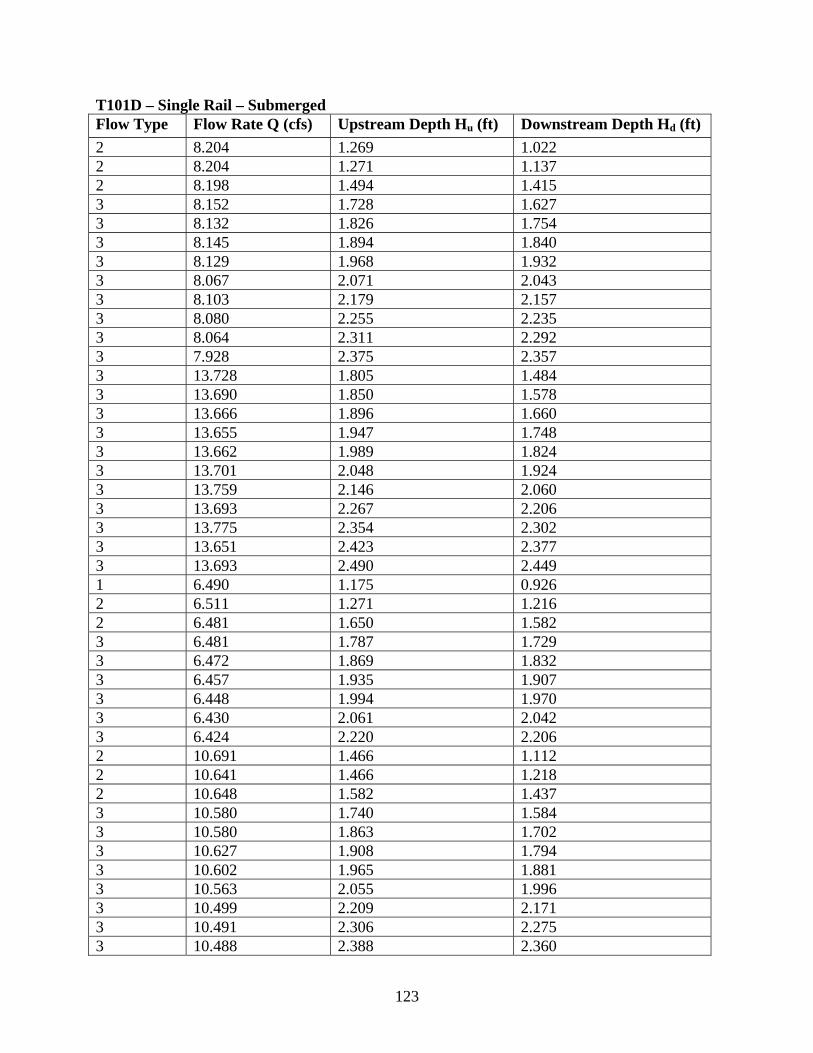
123

T101D – Single Rail – Submerged Flow Type Flow Rate Q (cfs) Upstream Depth Hu (ft) Downstream Depth Hd (ft) 2 8.204 1.269 1.022 2 8.204 1.271 1.137 2 8.198 1.494 1.415 3 8.152 1.728 1.627 3 8.132 1.826 1.754 3 8.145 1.894 1.840 3 8.129 1.968 1.932 3 8.067 2.071 2.043 3 8.103 2.179 2.157 3 8.080 2.255 2.235 3 8.064 2.311 2.292 3 7.928 2.375 2.357 3 13.728 1.805 1.484 3 13.690 1.850 1.578 3 13.666 1.896 1.660 3 13.655 1.947 1.748 3 13.662 1.989 1.824 3 13.701 2.048 1.924 3 13.759 2.146 2.060 3 13.693 2.267 2.206 3 13.775 2.354 2.302 3 13.651 2.423 2.377 3 13.693 2.490 2.449 1 6.490 1.175 0.926 2 6.511 1.271 1.216 2 6.481 1.650 1.582 3 6.481 1.787 1.729 3 6.472 1.869 1.832 3 6.457 1.935 1.907 3 6.448 1.994 1.970 3 6.430 2.061 2.042 3 6.424 2.220 2.206 2 10.691 1.466 1.112 2 10.641 1.466 1.218 2 10.648 1.582 1.437 3 10.580 1.740 1.584 3 10.580 1.863 1.702 3 10.627 1.908 1.794 3 10.602 1.965 1.881 3 10.563 2.055 1.996 3 10.499 2.209 2.171 3 10.491 2.306 2.275 3 10.488 2.388 2.360

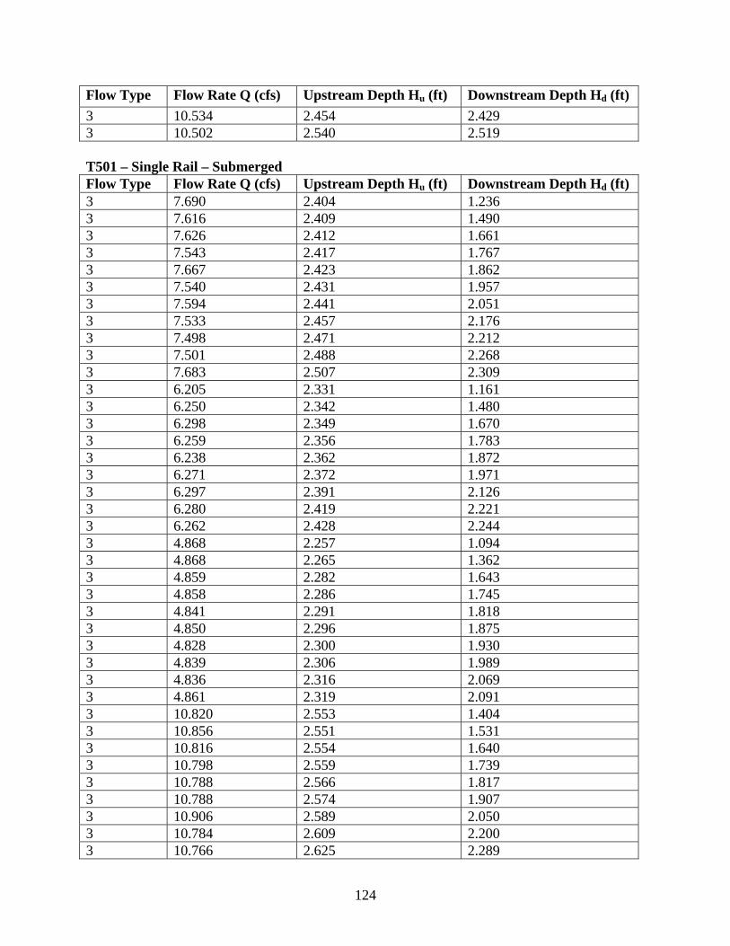
124

Flow Type Flow Rate Q (cfs) Upstream Depth Hu (ft) Downstream Depth Hd (ft) 3 10.534 2.454 2.429 3 10.502 2.540 2.519 T501 – Single Rail – Submerged Flow Type Flow Rate Q (cfs) Upstream Depth Hu (ft) Downstream Depth Hd (ft) 3 7.690 2.404 1.236 3 7.616 2.409 1.490 3 7.626 2.412 1.661 3 7.543 2.417 1.767 3 7.667 2.423 1.862 3 7.540 2.431 1.957 3 7.594 2.441 2.051 3 7.533 2.457 2.176 3 7.498 2.471 2.212 3 7.501 2.488 2.268 3 7.683 2.507 2.309 3 6.205 2.331 1.161 3 6.250 2.342 1.480 3 6.298 2.349 1.670 3 6.259 2.356 1.783 3 6.238 2.362 1.872 3 6.271 2.372 1.971 3 6.297 2.391 2.126 3 6.280 2.419 2.221 3 6.262 2.428 2.244 3 4.868 2.257 1.094 3 4.868 2.265 1.362 3 4.859 2.282 1.643 3 4.858 2.286 1.745 3 4.841 2.291 1.818 3 4.850 2.296 1.875 3 4.828 2.300 1.930 3 4.839 2.306 1.989 3 4.836 2.316 2.069 3 4.861 2.319 2.091 3 10.820 2.553 1.404 3 10.856 2.551 1.531 3 10.816 2.554 1.640 3 10.798 2.559 1.739 3 10.788 2.566 1.817 3 10.788 2.574 1.907 3 10.906 2.589 2.050 3 10.784 2.609 2.200 3 10.766 2.625 2.289

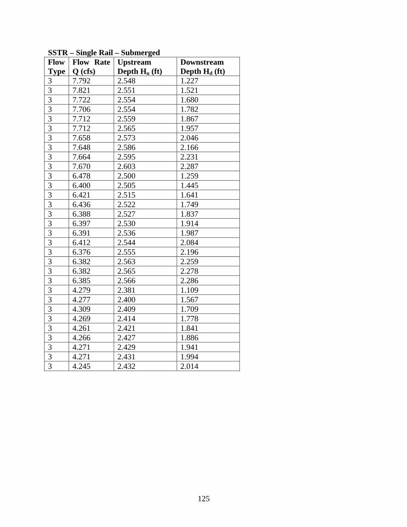
125

SSTR – Single Rail – Submerged Flow Type

Flow Rate Q (cfs)



3 7.792 2.548 1.227 3 7.821 2.551 1.521 3 7.722 2.554 1.680 3 7.706 2.554 1.782 3 7.712 2.559 1.867 3 7.712 2.565 1.957 3 7.658 2.573 2.046 3 7.648 2.586 2.166 3 7.664 2.595 2.231 3 7.670 2.603 2.287 3 6.478 2.500 1.259 3 6.400 2.505 1.445 3 6.421 2.515 1.641 3 6.436 2.522 1.749 3 6.388 2.527 1.837 3 6.397 2.530 1.914 3 6.391 2.536 1.987 3 6.412 2.544 2.084 3 6.376 2.555 2.196 3 6.382 2.563 2.259 3 6.382 2.565 2.278 3 6.385 2.566 2.286 3 4.279 2.381 1.109 3 4.277 2.400 1.567 3 4.309 2.409 1.709 3 4.269 2.414 1.778 3 4.261 2.421 1.841 3 4.266 2.427 1.886 3 4.271 2.429 1.941 3 4.271 2.431 1.994 3 4.245 2.432 2.014

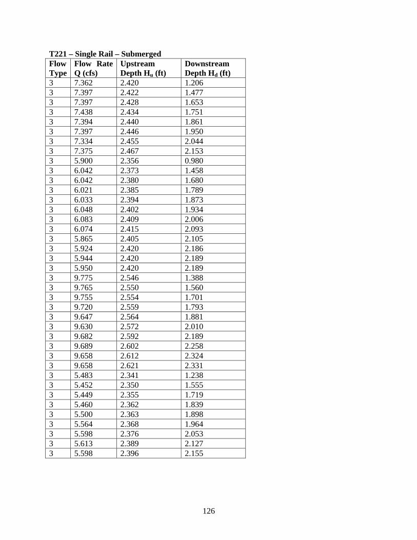
126


Flow Rate Q (cfs)



3 7.362 2.420 1.206 3 7.397 2.422 1.477 3 7.397 2.428 1.653 3 7.438 2.434 1.751 3 7.394 2.440 1.861 3 7.397 2.446 1.950 3 7.334 2.455 2.044 3 7.375 2.467 2.153 3 5.900 2.356 0.980 3 6.042 2.373 1.458 3 6.042 2.380 1.680 3 6.021 2.385 1.789 3 6.033 2.394 1.873 3 6.048 2.402 1.934 3 6.083 2.409 2.006 3 6.074 2.415 2.093 3 5.865 2.405 2.105 3 5.924 2.420 2.186 3 5.944 2.420 2.189 3 5.950 2.420 2.189 3 9.775 2.546 1.388 3 9.765 2.550 1.560 3 9.755 2.554 1.701 3 9.720 2.559 1.793 3 9.647 2.564 1.881 3 9.630 2.572 2.010 3 9.682 2.592 2.189 3 9.689 2.602 2.258 3 9.658 2.612 2.324 3 9.658 2.621 2.331 3 5.483 2.341 1.238 3 5.452 2.350 1.555 3 5.449 2.355 1.719 3 5.460 2.362 1.839 3 5.500 2.363 1.898 3 5.564 2.368 1.964 3 5.598 2.376 2.053 3 5.613 2.389 2.127 3 5.598 2.396 2.155

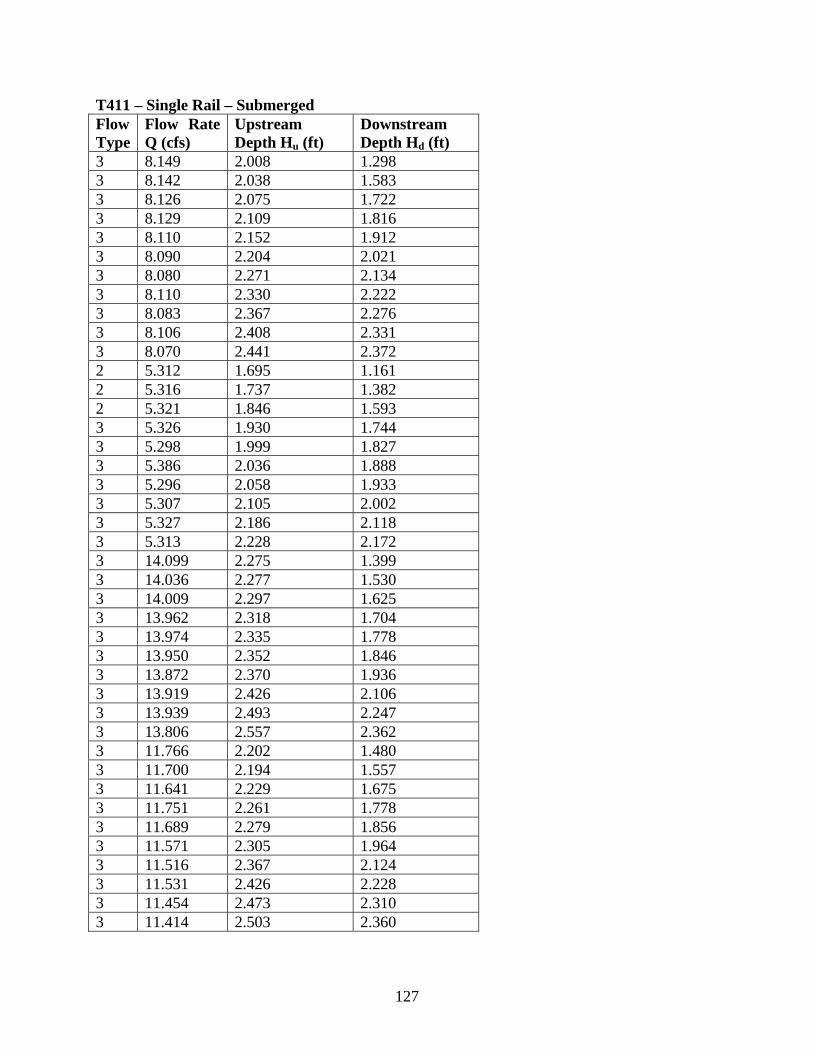
127


Flow Rate Q (cfs)



3 8.149 2.008 1.298 3 8.142 2.038 1.583 3 8.126 2.075 1.722 3 8.129 2.109 1.816 3 8.110 2.152 1.912 3 8.090 2.204 2.021 3 8.080 2.271 2.134 3 8.110 2.330 2.222 3 8.083 2.367 2.276 3 8.106 2.408 2.331 3 8.070 2.441 2.372 2 5.312 1.695 1.161 2 5.316 1.737 1.382 2 5.321 1.846 1.593 3 5.326 1.930 1.744 3 5.298 1.999 1.827 3 5.386 2.036 1.888 3 5.296 2.058 1.933 3 5.307 2.105 2.002 3 5.327 2.186 2.118 3 5.313 2.228 2.172 3 14.099 2.275 1.399 3 14.036 2.277 1.530 3 14.009 2.297 1.625 3 13.962 2.318 1.704 3 13.974 2.335 1.778 3 13.950 2.352 1.846 3 13.872 2.370 1.936 3 13.919 2.426 2.106 3 13.939 2.493 2.247 3 13.806 2.557 2.362 3 11.766 2.202 1.480 3 11.700 2.194 1.557 3 11.641 2.229 1.675 3 11.751 2.261 1.778 3 11.689 2.279 1.856 3 11.571 2.305 1.964 3 11.516 2.367 2.124 3 11.531 2.426 2.228 3 11.454 2.473 2.310 3 11.414 2.503 2.360

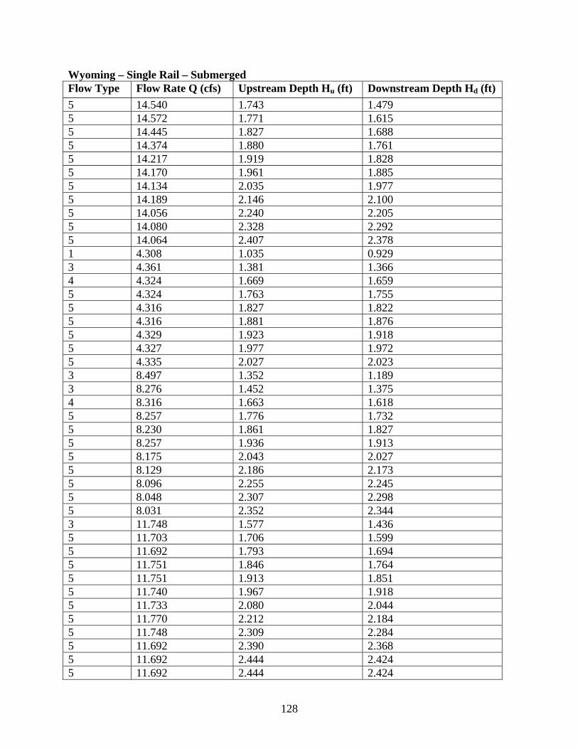
128

Wyoming – Single Rail – Submerged Flow Type Flow Rate Q (cfs) Upstream Depth Hu (ft) Downstream Depth Hd (ft) 5 14.540 1.743 1.479 5 14.572 1.771 1.615 5 14.445 1.827 1.688 5 14.374 1.880 1.761 5 14.217 1.919 1.828 5 14.170 1.961 1.885 5 14.134 2.035 1.977 5 14.189 2.146 2.100 5 14.056 2.240 2.205 5 14.080 2.328 2.292 5 14.064 2.407 2.378 1 4.308 1.035 0.929 3 4.361 1.381 1.366 4 4.324 1.669 1.659 5 4.324 1.763 1.755 5 4.316 1.827 1.822 5 4.316 1.881 1.876 5 4.329 1.923 1.918 5 4.327 1.977 1.972 5 4.335 2.027 2.023 3 8.497 1.352 1.189 3 8.276 1.452 1.375 4 8.316 1.663 1.618 5 8.257 1.776 1.732 5 8.230 1.861 1.827 5 8.257 1.936 1.913 5 8.175 2.043 2.027 5 8.129 2.186 2.173 5 8.096 2.255 2.245 5 8.048 2.307 2.298 5 8.031 2.352 2.344 3 11.748 1.577 1.436 5 11.703 1.706 1.599 5 11.692 1.793 1.694 5 11.751 1.846 1.764 5 11.751 1.913 1.851 5 11.740 1.967 1.918 5 11.733 2.080 2.044 5 11.770 2.212 2.184 5 11.748 2.309 2.284 5 11.692 2.390 2.368 5 11.692 2.444 2.424 5 11.692 2.444 2.424

129

Weir Rail – Single Rail – Submerged Flow Type

Flow Rate Q (cfs)



3 7.986 2.503 1.361 3 7.942 2.517 1.574 3 7.958 2.533 1.713 3 7.970 2.544 1.799 3 7.941 2.558 1.885 3 7.876 2.579 2.000 3 7.895 2.603 2.118 3 7.921 2.630 2.201 3 7.359 2.460 1.378 3 7.337 2.487 1.542 3 7.337 2.504 1.680 3 7.331 2.517 1.775 3 7.334 2.529 1.865 3 7.337 2.544 1.949 3 7.343 2.563 2.055 3 7.331 2.585 2.163 3 7.315 2.610 2.237 3 3.455 2.297 1.040 3 3.470 2.282 1.454 3 3.470 2.285 1.660 3 3.467 2.289 1.732 3 3.455 2.293 1.800 3 3.460 2.296 1.840 3 3.472 2.298 1.883 3 3.465 2.300 1.902 3 5.983 2.400 1.201 3 5.903 2.401 1.464 3 5.889 2.410 1.665 3 5.903 2.440 1.761 3 5.900 2.455 1.851 3 5.892 2.465 1.911 3 5.868 2.476 1.973 3 5.900 2.502 2.107 3 5.886 2.532 2.211 3 5.886 2.541 2.243 3 5.877 2.543 2.262

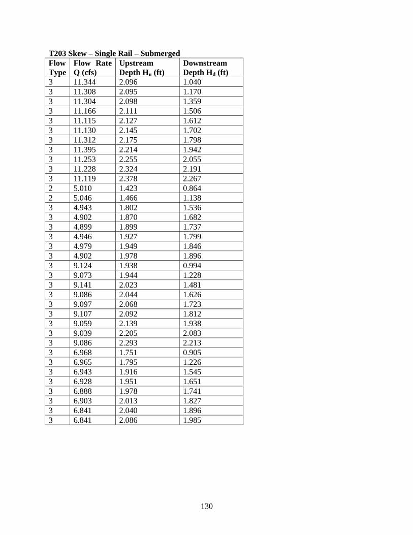
130

T203 Skew – Single Rail – Submerged Flow Type

Flow Rate Q (cfs)



3 11.344 2.096 1.040 3 11.308 2.095 1.170 3 11.304 2.098 1.359 3 11.166 2.111 1.506 3 11.115 2.127 1.612 3 11.130 2.145 1.702 3 11.312 2.175 1.798 3 11.395 2.214 1.942 3 11.253 2.255 2.055 3 11.228 2.324 2.191 3 11.119 2.378 2.267 2 5.010 1.423 0.864 2 5.046 1.466 1.138 3 4.943 1.802 1.536 3 4.902 1.870 1.682 3 4.899 1.899 1.737 3 4.946 1.927 1.799 3 4.979 1.949 1.846 3 4.902 1.978 1.896 3 9.124 1.938 0.994 3 9.073 1.944 1.228 3 9.141 2.023 1.481 3 9.086 2.044 1.626 3 9.097 2.068 1.723 3 9.107 2.092 1.812 3 9.059 2.139 1.938 3 9.039 2.205 2.083 3 9.086 2.293 2.213 3 6.968 1.751 0.905 3 6.965 1.795 1.226 3 6.943 1.916 1.545 3 6.928 1.951 1.651 3 6.888 1.978 1.741 3 6.903 2.013 1.827 3 6.841 2.040 1.896 3 6.841 2.086 1.985

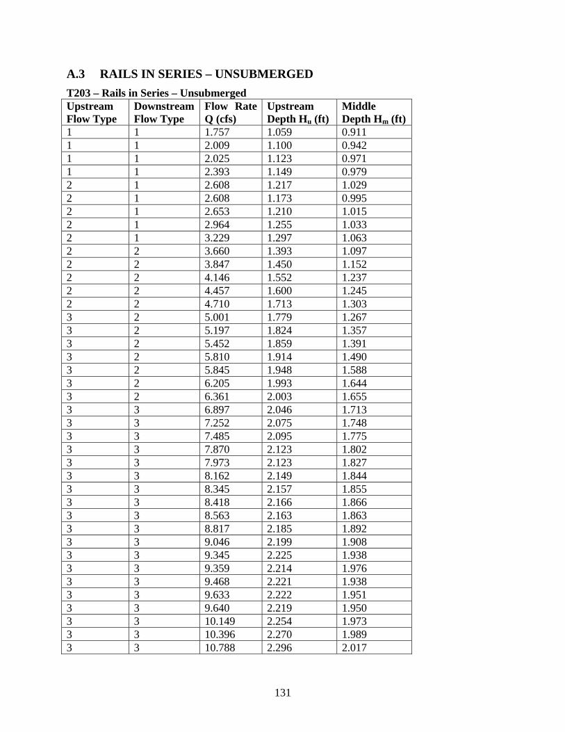
131

A.3 RAILS IN SERIES – UNSUBMERGED T203 – Rails in Series – Unsubmerged Upstream Flow Type

Downstream Flow Type

Flow RateQ (cfs)


Middle Depth Hm (ft)

1 1 1.757 1.059 0.911 1 1 2.009 1.100 0.942 1 1 2.025 1.123 0.971 1 1 2.393 1.149 0.979 2 1 2.608 1.217 1.029 2 1 2.608 1.173 0.995 2 1 2.653 1.210 1.015 2 1 2.964 1.255 1.033 2 1 3.229 1.297 1.063 2 2 3.660 1.393 1.097 2 2 3.847 1.450 1.152 2 2 4.146 1.552 1.237 2 2 4.457 1.600 1.245 2 2 4.710 1.713 1.303 3 2 5.001 1.779 1.267 3 2 5.197 1.824 1.357 3 2 5.452 1.859 1.391 3 2 5.810 1.914 1.490 3 2 5.845 1.948 1.588 3 2 6.205 1.993 1.644 3 2 6.361 2.003 1.655 3 3 6.897 2.046 1.713 3 3 7.252 2.075 1.748 3 3 7.485 2.095 1.775 3 3 7.870 2.123 1.802 3 3 7.973 2.123 1.827 3 3 8.162 2.149 1.844 3 3 8.345 2.157 1.855 3 3 8.418 2.166 1.866 3 3 8.563 2.163 1.863 3 3 8.817 2.185 1.892 3 3 9.046 2.199 1.908 3 3 9.345 2.225 1.938 3 3 9.359 2.214 1.976 3 3 9.468 2.221 1.938 3 3 9.633 2.222 1.951 3 3 9.640 2.219 1.950 3 3 10.149 2.254 1.973 3 3 10.396 2.270 1.989 3 3 10.788 2.296 2.017

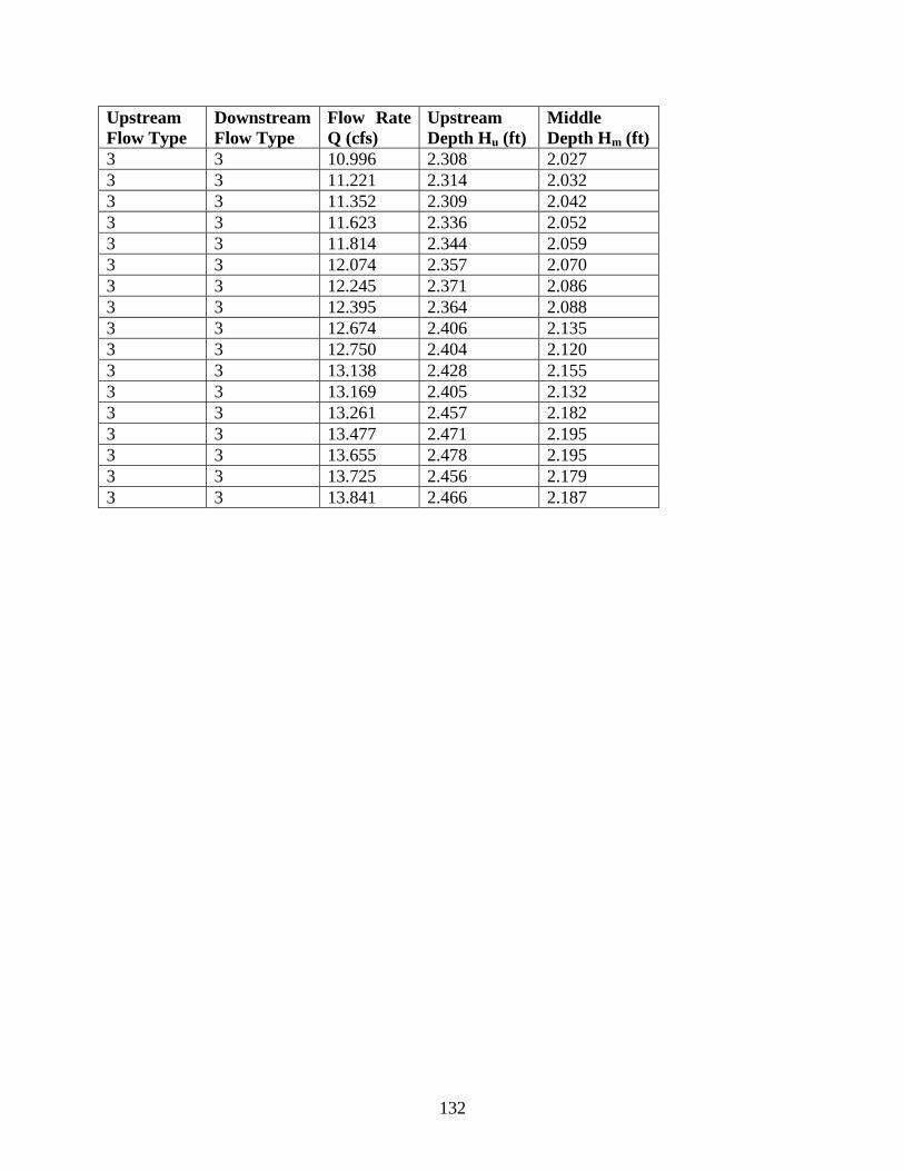
132

Upstream Flow Type


Flow RateQ (cfs)



3 3 10.996 2.308 2.027 3 3 11.221 2.314 2.032 3 3 11.352 2.309 2.042 3 3 11.623 2.336 2.052 3 3 11.814 2.344 2.059 3 3 12.074 2.357 2.070 3 3 12.245 2.371 2.086 3 3 12.395 2.364 2.088 3 3 12.674 2.406 2.135 3 3 12.750 2.404 2.120 3 3 13.138 2.428 2.155 3 3 13.169 2.405 2.132 3 3 13.261 2.457 2.182 3 3 13.477 2.471 2.195 3 3 13.655 2.478 2.195 3 3 13.725 2.456 2.179 3 3 13.841 2.466 2.187

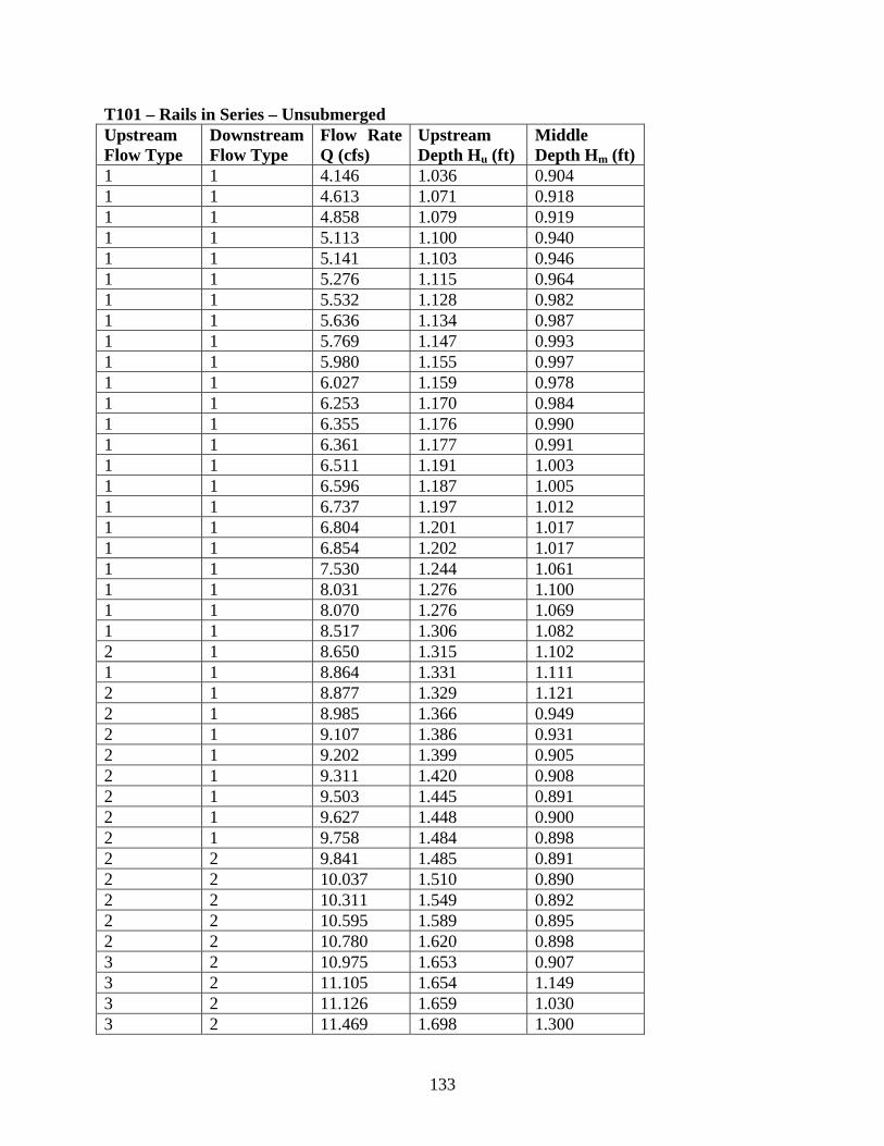
133

T101 – Rails in Series – Unsubmerged Upstream Flow Type


Flow RateQ (cfs)



1 1 4.146 1.036 0.904 1 1 4.613 1.071 0.918 1 1 4.858 1.079 0.919 1 1 5.113 1.100 0.940 1 1 5.141 1.103 0.946 1 1 5.276 1.115 0.964 1 1 5.532 1.128 0.982 1 1 5.636 1.134 0.987 1 1 5.769 1.147 0.993 1 1 5.980 1.155 0.997 1 1 6.027 1.159 0.978 1 1 6.253 1.170 0.984 1 1 6.355 1.176 0.990 1 1 6.361 1.177 0.991 1 1 6.511 1.191 1.003 1 1 6.596 1.187 1.005 1 1 6.737 1.197 1.012 1 1 6.804 1.201 1.017 1 1 6.854 1.202 1.017 1 1 7.530 1.244 1.061 1 1 8.031 1.276 1.100 1 1 8.070 1.276 1.069 1 1 8.517 1.306 1.082 2 1 8.650 1.315 1.102 1 1 8.864 1.331 1.111 2 1 8.877 1.329 1.121 2 1 8.985 1.366 0.949 2 1 9.107 1.386 0.931 2 1 9.202 1.399 0.905 2 1 9.311 1.420 0.908 2 1 9.503 1.445 0.891 2 1 9.627 1.448 0.900 2 1 9.758 1.484 0.898 2 2 9.841 1.485 0.891 2 2 10.037 1.510 0.890 2 2 10.311 1.549 0.892 2 2 10.595 1.589 0.895 2 2 10.780 1.620 0.898 3 2 10.975 1.653 0.907 3 2 11.105 1.654 1.149 3 2 11.126 1.659 1.030 3 2 11.469 1.698 1.300

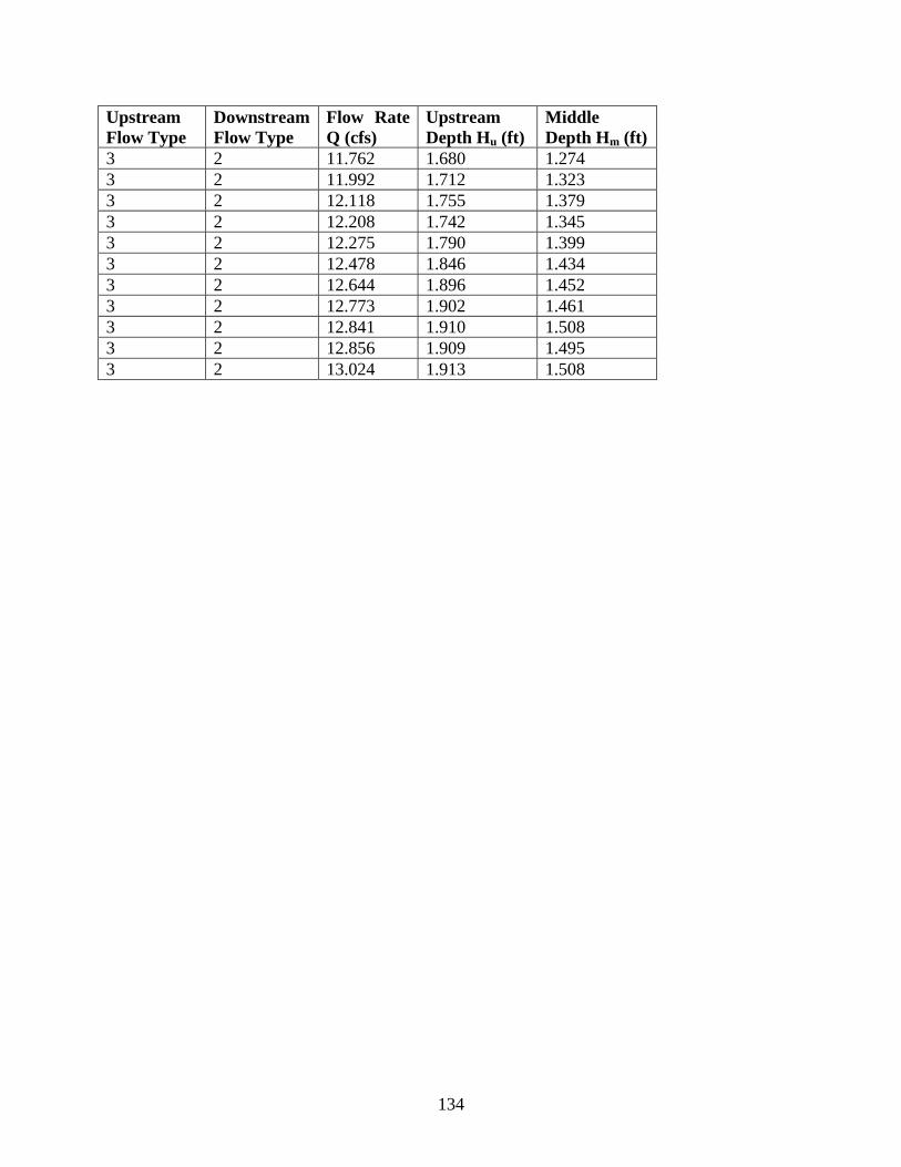
134

Upstream Flow Type


Flow RateQ (cfs)



3 2 11.762 1.680 1.274 3 2 11.992 1.712 1.323 3 2 12.118 1.755 1.379 3 2 12.208 1.742 1.345 3 2 12.275 1.790 1.399 3 2 12.478 1.846 1.434 3 2 12.644 1.896 1.452 3 2 12.773 1.902 1.461 3 2 12.841 1.910 1.508 3 2 12.856 1.909 1.495 3 2 13.024 1.913 1.508

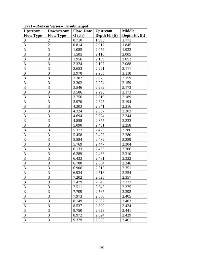
135

T221 – Rails in Series – Unsubmerged Upstream Flow Type


Flow RateQ (cfs)



3 2 0.710 1.993 1.771 3 2 0.814 2.017 1.845 3 3 1.085 2.059 1.923 3 3 1.505 2.116 2.005 3 3 1.956 2.159 2.052 3 3 2.324 2.197 2.088 3 3 2.653 2.221 2.111 3 3 2.978 2.238 2.118 3 3 3.302 2.273 2.159 3 3 3.302 2.274 2.159 3 3 3.546 2.292 2.173 3 3 3.586 2.293 2.173 3 3 3.756 2.310 2.189 3 3 3.970 2.325 2.194 3 3 4.203 2.341 2.216 3 3 4.324 2.337 2.203 3 3 4.694 2.374 2.244 3 3 4.858 2.375 2.233 3 3 5.090 2.401 2.258 3 3 5.372 2.423 2.286 3 3 5.458 2.427 2.280 3 3 5.584 2.432 2.289 3 3 5.769 2.447 2.304 3 3 6.133 2.463 2.306 3 3 6.289 2.466 2.310 3 3 6.433 2.481 2.322 3 3 6.780 2.504 2.346 3 3 6.906 2.513 2.351 3 3 6.934 2.518 2.354 3 3 7.202 2.525 2.357 3 3 7.479 2.540 2.373 3 3 7.511 2.542 2.375 3 3 7.709 2.567 2.392 3 3 7.973 2.580 2.405 3 3 8.149 2.582 2.403 3 3 8.537 2.609 2.424 3 3 8.750 2.629 2.441 3 3 8.972 2.624 2.429 3 3 9.379 2.660 2.461

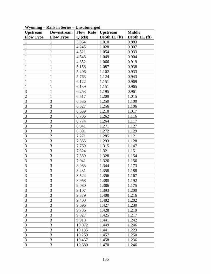
136

Wyoming – Rails in Series – Unsubmerged Upstream Flow Type


Flow RateQ (cfs)



1 1 3.954 1.010 0.883 1 1 4.245 1.028 0.907 1 1 4.521 1.054 0.933 1 1 4.548 1.049 0.904 1 1 4.852 1.066 0.919 1 1 5.158 1.087 0.938 1 1 5.406 1.102 0.933 1 1 5.763 1.124 0.943 1 1 6.122 1.151 0.969 1 1 6.139 1.151 0.965 3 1 6.253 1.195 0.961 2 1 6.517 1.208 1.015 3 3 6.536 1.250 1.100 3 3 6.627 1.256 1.106 3 3 6.639 1.218 1.017 3 3 6.706 1.262 1.116 3 3 6.774 1.264 1.117 3 3 6.841 1.271 1.127 3 3 6.891 1.272 1.129 3 2 7.271 1.285 1.121 3 3 7.365 1.293 1.128 3 3 7.760 1.315 1.147 3 3 7.824 1.321 1.151 3 3 7.889 1.328 1.154 3 3 7.941 1.326 1.156 3 3 8.083 1.344 1.173 3 3 8.431 1.358 1.188 3 3 8.524 1.356 1.167 3 3 8.958 1.380 1.192 3 3 9.080 1.386 1.175 3 3 9.107 1.393 1.200 3 3 9.379 1.408 1.216 3 3 9.400 1.402 1.202 3 3 9.696 1.427 1.230 3 3 9.786 1.428 1.219 3 3 9.827 1.425 1.217 3 3 9.918 1.441 1.242 3 3 10.072 1.449 1.246 3 3 10.135 1.441 1.223 3 3 10.269 1.457 1.250 3 3 10.467 1.458 1.236 3 3 10.680 1.470 1.246

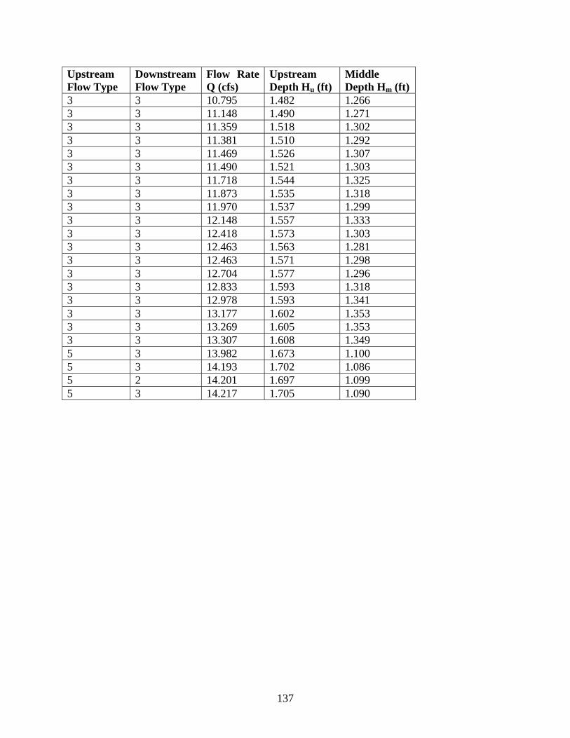
137

Upstream Flow Type


Flow RateQ (cfs)



3 3 10.795 1.482 1.266 3 3 11.148 1.490 1.271 3 3 11.359 1.518 1.302 3 3 11.381 1.510 1.292 3 3 11.469 1.526 1.307 3 3 11.490 1.521 1.303 3 3 11.718 1.544 1.325 3 3 11.873 1.535 1.318 3 3 11.970 1.537 1.299 3 3 12.148 1.557 1.333 3 3 12.418 1.573 1.303 3 3 12.463 1.563 1.281 3 3 12.463 1.571 1.298 3 3 12.704 1.577 1.296 3 3 12.833 1.593 1.318 3 3 12.978 1.593 1.341 3 3 13.177 1.602 1.353 3 3 13.269 1.605 1.353 3 3 13.307 1.608 1.349 5 3 13.982 1.673 1.100 5 3 14.193 1.702 1.086 5 2 14.201 1.697 1.099 5 3 14.217 1.705 1.090

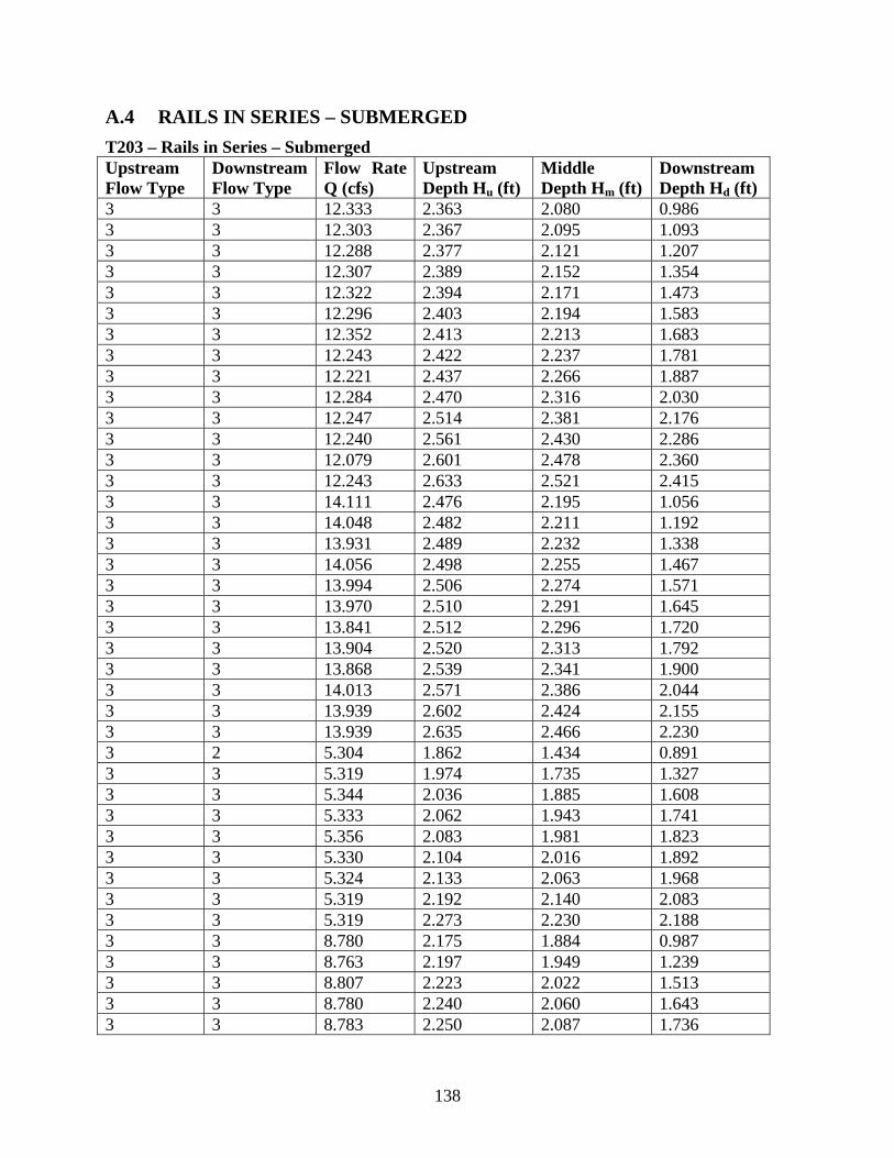
138

A.4 RAILS IN SERIES – SUBMERGED T203 – Rails in Series – Submerged Upstream Flow Type


Flow RateQ (cfs)




3 3 12.333 2.363 2.080 0.986 3 3 12.303 2.367 2.095 1.093 3 3 12.288 2.377 2.121 1.207 3 3 12.307 2.389 2.152 1.354 3 3 12.322 2.394 2.171 1.473 3 3 12.296 2.403 2.194 1.583 3 3 12.352 2.413 2.213 1.683 3 3 12.243 2.422 2.237 1.781 3 3 12.221 2.437 2.266 1.887 3 3 12.284 2.470 2.316 2.030 3 3 12.247 2.514 2.381 2.176 3 3 12.240 2.561 2.430 2.286 3 3 12.079 2.601 2.478 2.360 3 3 12.243 2.633 2.521 2.415 3 3 14.111 2.476 2.195 1.056 3 3 14.048 2.482 2.211 1.192 3 3 13.931 2.489 2.232 1.338 3 3 14.056 2.498 2.255 1.467 3 3 13.994 2.506 2.274 1.571 3 3 13.970 2.510 2.291 1.645 3 3 13.841 2.512 2.296 1.720 3 3 13.904 2.520 2.313 1.792 3 3 13.868 2.539 2.341 1.900 3 3 14.013 2.571 2.386 2.044 3 3 13.939 2.602 2.424 2.155 3 3 13.939 2.635 2.466 2.230 3 2 5.304 1.862 1.434 0.891 3 3 5.319 1.974 1.735 1.327 3 3 5.344 2.036 1.885 1.608 3 3 5.333 2.062 1.943 1.741 3 3 5.356 2.083 1.981 1.823 3 3 5.330 2.104 2.016 1.892 3 3 5.324 2.133 2.063 1.968 3 3 5.319 2.192 2.140 2.083 3 3 5.319 2.273 2.230 2.188 3 3 8.780 2.175 1.884 0.987 3 3 8.763 2.197 1.949 1.239 3 3 8.807 2.223 2.022 1.513 3 3 8.780 2.240 2.060 1.643 3 3 8.783 2.250 2.087 1.736

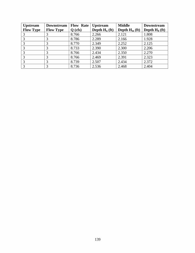
139

Upstream Flow Type


Flow RateQ (cfs)




3 3 8.766 2.266 2.121 1.808 3 3 8.786 2.289 2.166 1.928 3 3 8.770 2.349 2.252 2.125 3 3 8.733 2.390 2.300 2.206 3 3 8.766 2.434 2.350 2.270 3 3 8.766 2.469 2.391 2.323 3 3 8.739 2.507 2.434 2.372 3 3 8.736 2.536 2.468 2.404

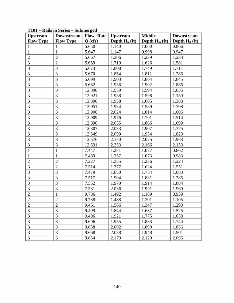
140

T101 – Rails in Series – Submerged Upstream Flow Type


Flow RateQ (cfs)




1 1 5.650 1.140 1.000 0.866 1 1 5.647 1.147 0.998 0.947 2 2 5.667 1.306 1.239 1.233 3 2 5.659 1.719 1.626 1.581 3 3 5.673 1.808 1.749 1.711 3 3 5.670 1.854 1.811 1.786 3 3 5.699 1.903 1.864 1.845 3 3 5.682 1.936 1.902 1.886 3 3 12.890 1.939 1.594 1.035 3 3 12.921 1.938 1.598 1.150 3 3 12.890 1.938 1.605 1.283 3 3 12.951 1.934 1.589 1.398 3 3 12.906 2.024 1.814 1.606 3 3 12.909 1.976 1.701 1.514 3 3 12.890 2.055 1.866 1.699 3 3 12.807 2.083 1.907 1.775 3 3 12.549 2.090 1.934 1.829 3 3 12.576 2.150 2.025 1.963 3 3 12.531 2.253 2.166 2.153 1 1 7.447 1.251 1.077 0.862 1 1 7.489 1.257 1.073 0.983 2 2 7.227 1.355 1.236 1.224 3 2 7.514 1.777 1.624 1.551 3 3 7.479 1.850 1.754 1.683 3 3 7.517 1.904 1.831 1.785 3 3 7.552 1.970 1.914 1.884 3 3 7.581 2.036 1.991 1.969 2 1 9.786 1.492 1.109 0.959 2 2 9.789 1.488 1.201 1.105 2 2 9.461 1.566 1.347 1.290 3 3 9.499 1.844 1.637 1.525 3 3 9.496 1.921 1.775 1.658 3 3 9.606 1.955 1.833 1.744 3 3 9.658 2.002 1.899 1.836 3 3 9.668 2.038 1.948 1.901 3 3 9.654 2.179 2.120 2.096

141

T221 – Rails in Series – Submerged Upstream Flow Type


Flow RateQ (cfs)




3 3 6.953 2.515 2.351 0.857 3 3 6.974 2.519 2.358 0.988 3 3 6.872 2.524 2.366 1.231 3 3 7.030 2.540 2.386 1.642 3 3 6.940 2.536 2.381 1.544 3 3 7.011 2.540 2.390 1.736 3 3 6.918 2.542 2.394 1.801 3 3 6.968 2.542 2.398 1.865 3 3 6.869 2.542 2.402 1.917 3 3 6.891 2.553 2.417 2.062 3 3 6.897 2.559 2.426 2.120 3 3 6.949 2.565 2.435 2.166 3 3 6.295 2.491 2.339 0.896 3 3 6.307 2.490 2.346 1.163 3 3 6.256 2.494 2.354 1.523 3 3 6.268 2.497 2.359 1.648 3 3 6.271 2.499 2.363 1.735 3 3 6.244 2.501 2.369 1.814 3 3 6.265 2.504 2.374 1.888 3 3 6.229 2.504 2.377 1.954 3 3 6.211 2.509 2.386 2.025 3 3 6.214 2.517 2.399 2.114 3 3 6.211 2.521 2.405 2.137 3 3 6.250 2.524 2.408 2.148 3 3 3.936 2.323 2.196 0.877 3 3 3.913 2.329 2.215 1.375 3 2 3.947 2.337 2.232 1.617 3 3 3.903 2.340 2.237 1.697 3 3 3.944 2.341 2.239 1.757 3 3 3.947 2.344 2.245 1.806 3 3 3.916 2.345 2.248 1.846 3 3 3.929 2.349 2.254 1.892 3 3 3.929 2.350 2.256 1.905 3 3 5.731 2.488 2.374 2.064 3 3 5.714 2.491 2.377 2.107 3 3 5.688 2.476 2.356 1.906 3 3 5.725 2.480 2.361 1.990 3 3 5.734 2.472 2.345 1.758 3 3 5.702 2.473 2.353 1.838 3 3 5.775 2.467 2.336 1.575 3 3 5.743 2.468 2.340 1.681 3 3 5.702 2.457 2.314 0.915

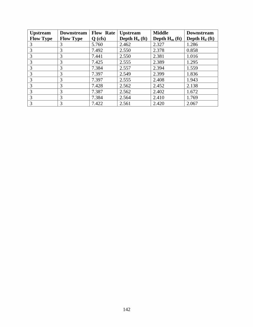
142

Upstream Flow Type


Flow RateQ (cfs)




3 3 5.760 2.462 2.327 1.286 3 3 7.492 2.550 2.378 0.858 3 3 7.441 2.550 2.381 1.016 3 3 7.425 2.555 2.389 1.295 3 3 7.384 2.557 2.394 1.559 3 3 7.397 2.549 2.399 1.836 3 3 7.397 2.555 2.408 1.943 3 3 7.428 2.562 2.452 2.138 3 3 7.387 2.562 2.402 1.672 3 3 7.384 2.564 2.410 1.769 3 3 7.422 2.561 2.420 2.067

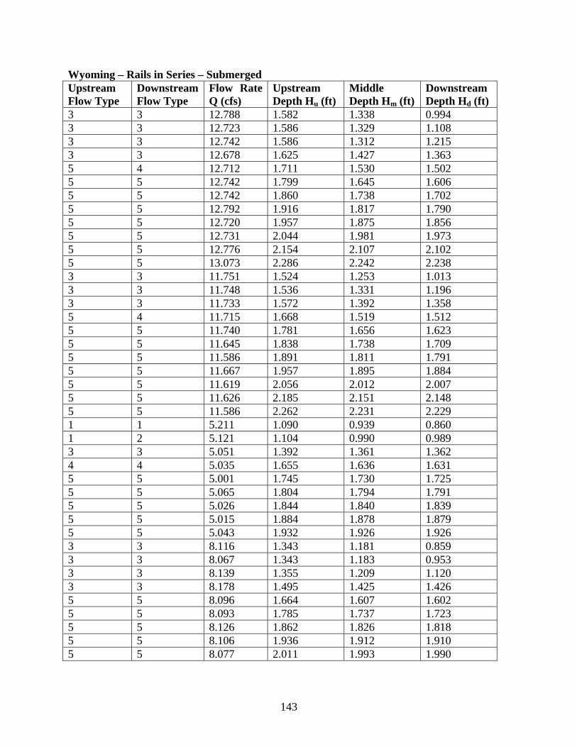
143

Wyoming – Rails in Series – Submerged Upstream Flow Type


Flow RateQ (cfs)




3 3 12.788 1.582 1.338 0.994 3 3 12.723 1.586 1.329 1.108 3 3 12.742 1.586 1.312 1.215 3 3 12.678 1.625 1.427 1.363 5 4 12.712 1.711 1.530 1.502 5 5 12.742 1.799 1.645 1.606 5 5 12.742 1.860 1.738 1.702 5 5 12.792 1.916 1.817 1.790 5 5 12.720 1.957 1.875 1.856 5 5 12.731 2.044 1.981 1.973 5 5 12.776 2.154 2.107 2.102 5 5 13.073 2.286 2.242 2.238 3 3 11.751 1.524 1.253 1.013 3 3 11.748 1.536 1.331 1.196 3 3 11.733 1.572 1.392 1.358 5 4 11.715 1.668 1.519 1.512 5 5 11.740 1.781 1.656 1.623 5 5 11.645 1.838 1.738 1.709 5 5 11.586 1.891 1.811 1.791 5 5 11.667 1.957 1.895 1.884 5 5 11.619 2.056 2.012 2.007 5 5 11.626 2.185 2.151 2.148 5 5 11.586 2.262 2.231 2.229 1 1 5.211 1.090 0.939 0.860 1 2 5.121 1.104 0.990 0.989 3 3 5.051 1.392 1.361 1.362 4 4 5.035 1.655 1.636 1.631 5 5 5.001 1.745 1.730 1.725 5 5 5.065 1.804 1.794 1.791 5 5 5.026 1.844 1.840 1.839 5 5 5.015 1.884 1.878 1.879 5 5 5.043 1.932 1.926 1.926 3 3 8.116 1.343 1.181 0.859 3 3 8.067 1.343 1.183 0.953 3 3 8.139 1.355 1.209 1.120 3 3 8.178 1.495 1.425 1.426 5 5 8.096 1.664 1.607 1.602 5 5 8.093 1.785 1.737 1.723 5 5 8.126 1.862 1.826 1.818 5 5 8.106 1.936 1.912 1.910 5 5 8.077 2.011 1.993 1.990

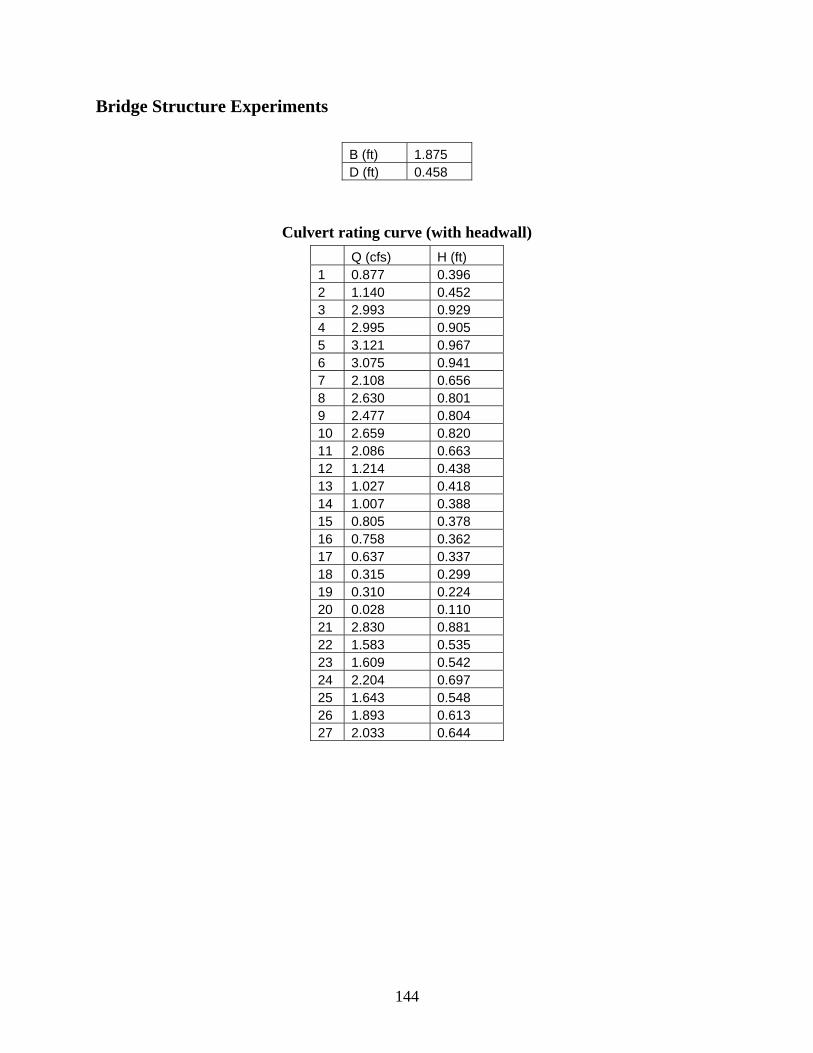
144

Bridge Structure Experiments

B (ft) 1.875 D (ft) 0.458

Culvert rating curve (with headwall) Q (cfs) H (ft)

1 0.877 0.396 2 1.140 0.452 3 2.993 0.929 4 2.995 0.905 5 3.121 0.967 6 3.075 0.941 7 2.108 0.656 8 2.630 0.801 9 2.477 0.804 10 2.659 0.820 11 2.086 0.663 12 1.214 0.438 13 1.027 0.418 14 1.007 0.388 15 0.805 0.378 16 0.758 0.362 17 0.637 0.337 18 0.315 0.299 19 0.310 0.224 20 0.028 0.110 21 2.830 0.881 22 1.583 0.535 23 1.609 0.542 24 2.204 0.697 25 1.643 0.548 26 1.893 0.613 27 2.033 0.644

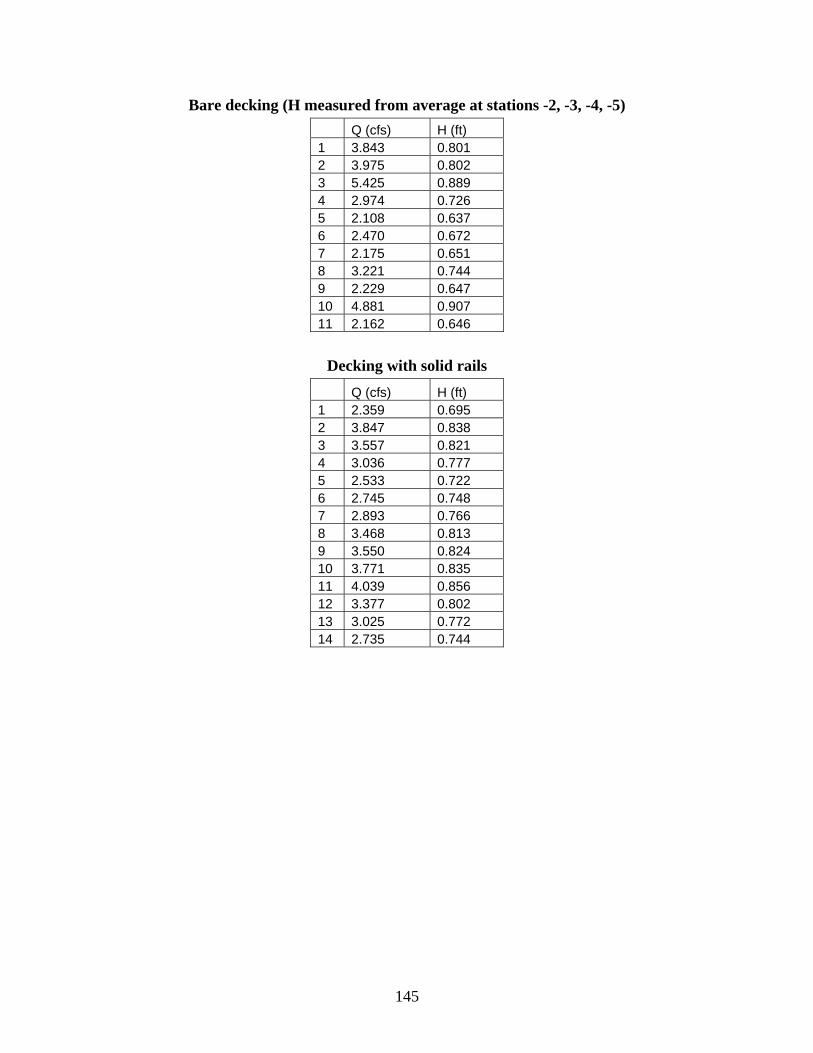
145

Bare decking (H measured from average at stations -2, -3, -4, -5) Q (cfs) H (ft)

1 3.843 0.801 2 3.975 0.802 3 5.425 0.889 4 2.974 0.726 5 2.108 0.637 6 2.470 0.672 7 2.175 0.651 8 3.221 0.744 9 2.229 0.647 10 4.881 0.907 11 2.162 0.646

Decking with solid rails Q (cfs) H (ft)

1 2.359 0.695 2 3.847 0.838 3 3.557 0.821 4 3.036 0.777 5 2.533 0.722 6 2.745 0.748 7 2.893 0.766 8 3.468 0.813 9 3.550 0.824 10 3.771 0.835 11 4.039 0.856 12 3.377 0.802 13 3.025 0.772 14 2.735 0.744

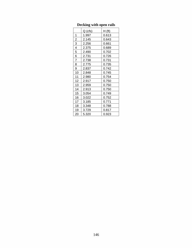
146

Decking with open rails Q (cfs) H (ft)

1 1.997 0.613 2 2.145 0.643 3 2.256 0.661 4 2.375 0.689 5 2.490 0.702 6 2.731 0.726 7 2.738 0.731 8 2.775 0.735 9 2.837 0.742 10 2.848 0.745 11 2.980 0.754 12 2.917 0.750 13 2.959 0.750 14 2.913 0.750 15 3.054 0.749 16 3.022 0.752 17 3.185 0.771 18 3.348 0.788 19 3.729 0.817 20 5.320 0.923

Documents

Hydraulic Performance of Bridge Rails (FHWA/TX-09/0 … · • Hydraulic Performance of Bridge Rails based on Rating Curves and Submergence ... 3.2.2 Methodology ... Experiment Results