NREL is a national laboratory of the U.S. Department of Energy Office of Energy Efficiency & Renewable Energy Operated by the Alliance for Sustainable Energy, LLC

This report is available at no cost from the National Renewable Energy Laboratory (NREL) at www.nrel.gov/publications.

Contract No. DE-AC36-08GO28308

HydroDyn User’s Guide and Theory Manual J.M. Jonkman, A.N. Robertson, G.J. Hayman NREL

Technical Report (Arial 11 pt Bold) NREL/TP-xxxx-xxxxx Month Year (Arial 11 pt)

NREL is a national laboratory of the U.S. Department of Energy Office of Energy Efficiency & Renewable Energy Operated by the Alliance for Sustainable Energy, LLC

This report is available at no cost from the National Renewable Energy Laboratory (NREL) at www.nrel.gov/publications.

Contract No. DE-AC36-08GO28308

National Renewable Energy Laboratory 15013 Denver West Parkway Golden, CO 80401 303-275-3000 • www.nrel.gov

HydroDyn User’s Guide and Theory Manual J.M. Jonkman, A.N. Robertson, G.J. Hayman NREL

Prepared under Task No(s). XXXX.XXXX, XXXX.XXXX

Technical Report (Arial 11 pt Bold) NREL/TP-xxxx-xxxxx Month Year (Arial 11 pt)

NOTICE

This report was prepared as an account of work sponsored by an agency of the United States government. Neither the United States government nor any agency thereof, nor any of their employees, makes any warranty, express or implied, or assumes any legal liability or responsibility for the accuracy, completeness, or usefulness of any information, apparatus, product, or process disclosed, or represents that its use would not infringe privately owned rights. Reference herein to any specific commercial product, process, or service by trade name, trademark, manufacturer, or otherwise does not necessarily constitute or imply its endorsement, recommendation, or favoring by the United States government or any agency thereof. The views and opinions of authors expressed herein do not necessarily state or reflect those of the United States government or any agency thereof.

This report is available at no cost from the National Renewable Energy Laboratory (NREL) at www.nrel.gov/publications.

Available electronically at http://www.osti.gov/scitech

Available for a processing fee to U.S. Department of Energy and its contractors, in paper, from:

U.S. Department of Energy Office of Scientific and Technical Information P.O. Box 62 Oak Ridge, TN 37831-0062 phone: 865.576.8401 fax: 865.576.5728 email: mailto:reports@adonis.osti.gov

Available for sale to the public, in paper, from:

U.S. Department of Commerce National Technical Information Service 5285 Port Royal Road Springfield, VA 22161 phone: 800.553.6847 fax: 703.605.6900 email: orders@ntis.fedworld.gov online ordering: http://www.ntis.gov/help/ordermethods.aspx

Cover Photos: (left to right) photo by Pat Corkery, NREL 16416, photo from SunEdison, NREL 17423, photo by Pat Corkery, NREL 16560, photo by Dennis Schroeder, NREL 17613, photo by Dean Armstrong, NREL 17436, photo by Pat Corkery, NREL 17721.

Printed on paper containing at least 50% wastepaper, including 10% post consumer waste.

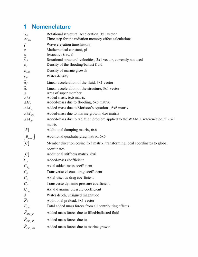
1 Nomenclature Sα

Rotational structural acceleration, 3x1 vector RDt∆ Time step for the radiation memory effect calculations

ζ Wave elevation time history π Mathematical constant, pi ω frequency (rad/s)

Sω

Rotational structural velocities, 3x1 vector, currently not used fρ Density of the flooding/ballast fluid

MGρ Density of marine growth

Wρ Water density

fa

Linear acceleration of the fluid, 3x1 vector sa

Linear acceleration of the structure, 3x1 vector A Area of super member AM Added-mass, 6x6 matrix

FAM Added-mass due to flooding, 6x6 matrix

MAM Added-mass due to Morison’s equations, 6x6 matrix

MGAM Added-mass due to marine growth, 6x6 matrix

RPAM Added-mass due to radiation problem applied to the WAMIT reference point, 6x6 matrix

[ ]B Additional damping matrix, 6x6

quadB Additional quadratic drag matrix, 6x6

[ ]C Member direction cosine 3x3 matrix, transforming local coordinates to global coordinates

[ ]C Additional stiffness matrix, 6x6

AC Added-mass coefficient

AxAC Axial added-mass coefficient

DC Transverse viscous-drag coefficient

AxDC Axial viscous-drag coefficient

PC Transverse dynamic pressure coefficient

AxPC Axial dynamic pressure coefficient d Water depth, unsigned magnitude

0F

Additional preload, 3x1 vector

AMF

Total added mass forces from all contributing effects

_AM FF

Added mass forces due to filled/ballasted fluid

_AM MF

Added mass forces due to

_AM MGF

Added mass forces due to marine growth

jF

Total forces and moments applied to node j, 6x1 vector ADDF

Total loads due to preload, additional stiffness, and additional damping terms, 6x1 vector

BF

Buoyancy forces and moments applied to node, 6x1 vector DF

Drag forces and moments applied to node, 6x1 vector _F BF

Buoyancy forces and moments due to flooding applied to node, 6x1 vector HSF

Hydrostatic forces applied to the platform reference node, 6x1 vector IF

Inertial forces and moments applied to node, 6x1 vector MGF

Marine growth-related forces and moments applied to node, 6x1 vector RDF

Radiation memory-effect force applied to platform reference point, 6x1 vector WF

Incident-wave excitation force applied to platform reference point, 6x1 vector

glbiF

Point buoyancy forces at the end cap of the ith member which connects to the super member

WF

Incident-wave excitation force applied to platform reference point, 6x1 vector WRPF

Total loads at the WAMIT reference point from potential flow theory, 6x1 vector g Gravity, unsigned magnitude

refh Reference depth for the near-surface current model i member or element index i Unit vector along the local x-axis I Unit vector along the global X-axis j node index, imaginary number constant

j Unit vector along the local y-axis J Unit vector along the global Y-axis k Unit vector along the local z-axis K Radiation kernel from potential flow theory, 6x6 matrix K Unit vector along the global Z-axis kg Kilograms

mL Length of master cylinder of a super member

isL Length of the ith slave cylinder of a super member m Meters M Number of members connected to a given joint n the nth time step ˆin Outward facing normal for member the ith member. Parallel to the local k axis N Newtons

dynp Fluid dynamic pressure R Outer radius of structural member

mR Outer radius of the super member’s master cylinder

isR Outer radius of the ith slave cylinder which is part of a super member

s seconds t time

Mt Thickness of structural member

Met Thickness of structural member at element end

mMGt Marine-growth thickness on the master cylinder

siMGt Marine-growth thickness on ith slave cylinder of a super member

Mst Thickness of structural member at element start

MGt Marine-growth thickness

0NSU Reference current velocity for the near-surface current model

0SSU Reference current velocity for the sub-surface current model

NSU Current velocity at depth, Z, for the near-surface current model

SSU Current velocity at depth, Z, for the sub-surface current model

fv

Linear velocity of the fluid, 3x1 vector relv

Relative velocity, rel f sv v v= − 3x1 vector

Sv

Translational structural velocities, 3x1 vector V Volume of member (super member)

ciV Volume of ith cylinder which is a part of the super member

IV Interior cavity volume of member (super member)

MGV added volume due to marine growth Tx y z Position in the local, member coordinate system

TX Y Z Position in the global, inertial coordinate system dnx Discrete states of the radiation solution

HXD Radiation damping history

2 Introduction HydroDyn is a time-domain hydrodynamics module that has been coupled into the FAST wind turbine computer-aided engineering (CAE) tool to enable aero-hydro-servo-elastic simulation of offshore wind turbines. HydroDyn is applicable to both fixed-bottom and floating offshore substructures. This latest release of HydroDyn follows the requirements of the FAST modularization framework and couples to FAST version 8. HydroDyn can also be driven as a standalone code to compute hydrodynamic loading uncoupled from FAST.

HydroDyn allows for multiple approaches for calculating the hydrodynamic loads on a structure: a potential-flow theory solution, a strip-theory solution, or a combination of the two. Waves in HydroDyn can be regular (periodic) or irregular (stochastic) and long-crested (unidirectional) or short-crested (with wave energy spread across a range of directions). HydroDyn treats waves using first-order (linear Airy) or first- plus second-order wave theory [Sharma and Dean, 1981] with the option to include directional spreading, but no wave stretching or higher order wave theories are included. The second-order hydrodynamic implementations are new in this release and include time-domain calculations of difference- (mean- and slow-drift-) and sum-frequency terms. To minimize computational expense, Fast Fourier Transforms (FFTs) are applied in the summation of all wave frequency components.

The potential-flow solution is applicable to substructures or members of substructures that are large relative to a typical wavelength. Potential-flow hydrodynamic loads include linear hydrostatic restoring, the added mass and damping contributions from linear wave radiation (including free-surface memory effects), and the incident-wave excitation from first- and second-order diffraction. The hydrodynamic coefficients (first and second order) required for the potential-flow solution are frequency dependent and must be supplied by a separate frequency-domain panel code (e.g., WAMIT) from a pre-computation step. The radiation memory effect can be calculated either through direct time-domain convolution or through a linear state-space approach, with a state-space model derived through the SS_Fitting preprocessor. The second-order terms can be derived from the full difference- and sum-frequency quadratic transfer functions (QTFs) or the difference-frequency terms can be estimated via Standing et al.’s extension to Newman’s approximation, based only on first-order coefficients.

The strip-theory solution may be preferable for substructures or members of substructures that are small in diameter relative to a typical wavelength. Strip-theory hydrodynamic loads can be applied across multiple interconnected members, each with possible incline and taper, and are derived directly from the undisturbed wave and current kinematics at the undisplaced position of the substructure. The undisturbed first- and second-order wave kinematics are implemented analytically for finite depth. The strip-theory loads include the relative form of Morison’s equation for the distributed fluid-inertia, added-mass, and viscous-drag components. Additional distributed load components include axial loads from tapered members and static buoyancy loads. Hydrodynamic loads are also applied as lumped loads on member endpoints (called joints). It is also possible to include flooding or ballasting of members, and the effects of marine growth. The hydrodynamic coefficients required for this solution come through user-specified dynamic-pressure, added-mass, and viscous-drag coefficients.

For some substructures and sea conditions, the hydrodynamic loads from a potential-flow theory must be augmented with the loads brought about by flow separation. For this, the viscous-drag component of the strip-theory solution may be included with the potential-flow theory solution. Another option available is to supply a global damping matrix (linear or quadratic) to the system to represent this effect.

When HydroDyn is coupled to FAST, HydroDyn receives the position, orientation, velocities, and accelerations of the (rigid or flexible) substructure at each coupling time step and then computes the hydrodynamic loads and returns them back to FAST. At this time, FAST’s ElastoDyn structural-dynamics module assumes for a floating platform that the substructure (floating platform) is a six degree-of-freedom (DOF) rigid body. For fixed-bottom offshore wind turbines, FAST’s SubDyn module allows for structural flexibility of multi-member substructures and the coupling to HydroDyn includes hydro-elastic effects.

The primary HydroDyn input file defines the substructure geometry, hydrodynamic coefficients, incident wave kinematics and current, potential-flow solution options, flooding/ballasting and marine growth, and auxiliary parameters. The geometry of strip-theory members is defined by joint coordinates of the undisplaced substructure in the global reference system, with the origin at the intersection of the undeflected tower centerline with mean sea level (MSL). A member connects two joints; multiple members can use a common joint. The hydrodynamic loads are computed at nodes, which are the resultant of member refinement into multiple (MDivSize input) elements (nodes are located at the ends of each element), and they are calculated by the module. Member properties include outer diameter, thickness, and dynamic-pressure, added-mass and viscous-drag coefficients. Member properties are specified at the joints; if properties change from one joint to the other, they will be linearly interpolated for the inner nodes.

Section 3 details how to obtain the HydroDyn and FAST software archives and how to run both the stand-alone HydroDyn or HydroDyn coupled to FAST. Section 4 describes the HydroDyn input files. Section 5 discusses the output files generated by HydroDyn; these include echo files, wave-elevation outputs, a summary file, and the results file. Section 6 provides modeling guidance when using HydroDyn. The HydroDyn theory is covered in Section 7. Section 8 outlines future work, and Section 9 contains a list of references. Example input files are shown in Appendix A and B. A summary of available output channels are found in Appendix C. Instructions for compiling the stand-alone HydroDyn program are detailed in Appendix D. Appendix E tracks the major changes we have made to HydroDyn for each public release.

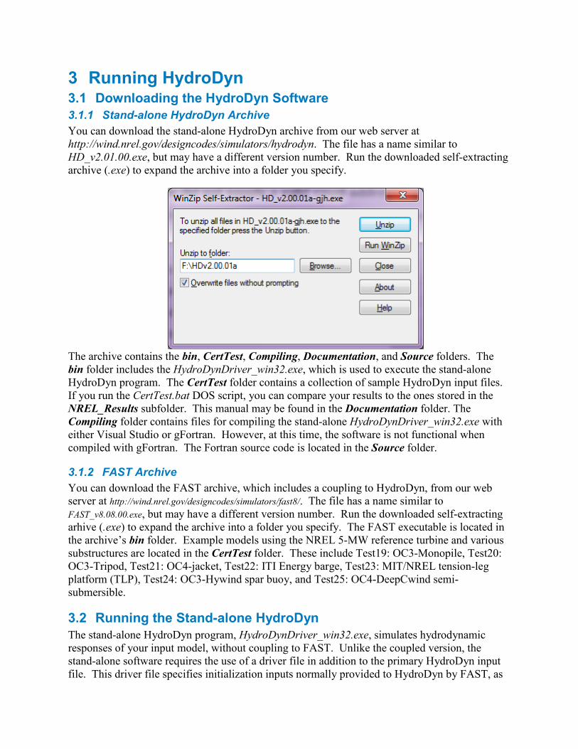
3 Running HydroDyn 3.1 Downloading the HydroDyn Software 3.1.1 Stand-alone HydroDyn Archive You can download the stand-alone HydroDyn archive from our web server at http://wind.nrel.gov/designcodes/simulators/hydrodyn. The file has a name similar to HD_v2.01.00.exe, but may have a different version number. Run the downloaded self-extracting archive (.exe) to expand the archive into a folder you specify.

The archive contains the bin, CertTest, Compiling, Documentation, and Source folders. The bin folder includes the HydroDynDriver_win32.exe, which is used to execute the stand-alone HydroDyn program. The CertTest folder contains a collection of sample HydroDyn input files. If you run the CertTest.bat DOS script, you can compare your results to the ones stored in the NREL_Results subfolder. This manual may be found in the Documentation folder. The Compiling folder contains files for compiling the stand-alone HydroDynDriver_win32.exe with either Visual Studio or gFortran. However, at this time, the software is not functional when compiled with gFortran. The Fortran source code is located in the Source folder.

3.1.2 FAST Archive You can download the FAST archive, which includes a coupling to HydroDyn, from our web server at http://wind.nrel.gov/designcodes/simulators/fast8/. The file has a name similar to FAST_v8.08.00.exe, but may have a different version number. Run the downloaded self-extracting arhive (.exe) to expand the archive into a folder you specify. The FAST executable is located in the archive’s bin folder. Example models using the NREL 5-MW reference turbine and various substructures are located in the CertTest folder. These include Test19: OC3-Monopile, Test20: OC3-Tripod, Test21: OC4-jacket, Test22: ITI Energy barge, Test23: MIT/NREL tension-leg platform (TLP), Test24: OC3-Hywind spar buoy, and Test25: OC4-DeepCwind semi-submersible.

3.2 Running the Stand-alone HydroDyn The stand-alone HydroDyn program, HydroDynDriver_win32.exe, simulates hydrodynamic responses of your input model, without coupling to FAST. Unlike the coupled version, the stand-alone software requires the use of a driver file in addition to the primary HydroDyn input file. This driver file specifies initialization inputs normally provided to HydroDyn by FAST, as

well as the per-time-step inputs to HydroDyn. Both the HydroDyn summary file and the results output file are available when using the stand-alone HydroDyn, see Section 5 for more information regarding the HydroDyn output files.

Run the standalone HydroDyn software from a DOS command prompt by typing, e.g.

>HydroDynDriver_win32.exe MyDriverFile.dvr

where, MyDriverFile.dvr is the name of the HydroDyn driver file, as described in Section 4.2. The HydroDyn primary input file is described in Section 4.3.

3.3 Running HydroDyn Coupled to FAST Run the coupled FAST software from a DOS command prompt by typing, e.g.

>FAST_win32.exe Test22.fst

where, Test22.fst is the name of the primary FAST input file. This input file has a control flag to turn on or off the HydroDyn capabilities within FAST, and a corresponding reference to the HydroDyn input file. See the documentation supplied with FAST for further information.

4 Input Files The user configures the hydrodynamic model parameters as well as the substructure geometry and properties via a primary HydroDyn input file. When used in stand-alone mode, an additional driver input file is required. This driver file specifies initialization inputs normally provided to HydroDyn by FAST, as well as the per-time-step inputs to HydroDyn.

No lines should be added or removed from the input files, except in tables where the number of rows is specified.

4.1 Units HydroDyn uses the SI system (kg, m, s, N).

4.2 HydroDyn Driver Input File The driver input file is only needed for the stand-alone version of HydroDyn and contains inputs normally generated by FAST, and are necessary to control the hydrodynamic simulation for uncoupled models. A sample HydroDyn driver input file is given in Appendix B.

Set the Echo flag in this file to TRUE if you wish to have HydroDynDriver.exe echo the contents of the driver input file (useful for debugging errors in the driver file). The echo file has the naming convention of OutRootName.dvr.ech. OutRootName is specified in the HYDRODYN section of the driver input file. Set the gravity constant using the Gravity parameter. HydroDyn expects a magnitude, so in SI units this would be set to 9.80665 𝑚

𝑠2. HDInputFile is the filename

of the primary HydroDyn input file. This name should be in quotations and can contain an absolute path or a relative path. All HydroDyn-generated output files will be prefixed with OutRootName. If this parameter includes a filepath, the output will be generated in that folder. NSteps specifies the number of simulation time steps, and TimeInterval specifies the time between steps.

Setting WAMITInputsMod = 0 forces all WAMIT reference point (WRP) input motions to zero for all time. If you set WAMITInputsMod = 1, then you must set the steady-state inputs in the WAMIT STEADY STATE INPUTS section of the file. Setting WAMITInputsMod = 2, requires the time-series input file whose name is specified via the WAMITInputsFile parameter. The WAMIT inputs file is a text-formatted file. This file has no header lines. Each data row corresponds to a given time step, and the whitespace separated columns of floating point values represent the necessary motion inputs as shown in Table 1. All motions are specified in the global inertial-frame coordinate system.

Table 1. WAMIT Inputs Time-Series Data File Contents

Column Number Input Units

1 Time step value 𝑠

2-4 Translational displacements along X, Y, and Z

𝑚

5-7 Rotational displacements about X, Y, and Z (small angle

𝑟𝑎𝑑𝑖𝑎𝑛𝑠

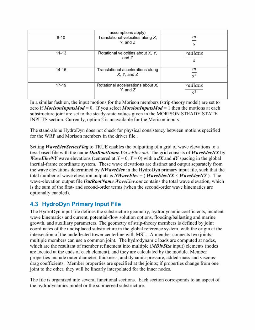
assumptions apply) 8-10 Translational velocities along X,

Y, and Z 𝑚𝑠

11-13 Rotational velocities about X, Y, and Z

𝑟𝑎𝑑𝑖𝑎𝑛𝑠𝑠

14-16 Translational accelerations along X, Y, and Z

𝑚𝑠2

17-19 Rotational accelerations about X, Y, and Z

𝑟𝑎𝑑𝑖𝑎𝑛𝑠𝑠2

In a similar fashion, the input motions for the Morison members (strip-theory model) are set to zero if MorisonInputsMod = 0. If you select MorsionInputsMod = 1 then the motions at each substructure joint are set to the steady-state values given in the MORISON STEADY STATE INPUTS section. Currently, option 2 is unavailable for the Morison inputs.

The stand-alone HydroDyn does not check for physical consistency between motions specified for the WRP and Morison members in the driver file .

Setting WaveElevSeriesFlag to TRUE enables the outputting of a grid of wave elevations to a text-based file with the name OutRootName.WaveElev.out. The grid consists of WaveElevNX by WaveElevNY wave elevations (centered at X = 0, Y = 0) with a dX and dY spacing in the global inertial-frame coordinate system. These wave elevations are distinct and output separately from the wave elevations determined by NWaveElev in the HydroDyn primary input file, such that the total number of wave elevation outputs is NWaveElev + ( WaveElevNX × WaveElevNY ). The wave-elevation output file OutRootName.WaveElev.out contains the total wave elevation, which is the sum of the first- and second-order terms (when the second-order wave kinematics are optionally enabled).

4.3 HydroDyn Primary Input File The HydroDyn input file defines the substructure geometry, hydrodynamic coefficients, incident wave kinematics and current, potential-flow solution options, flooding/ballasting and marine growth, and auxiliary parameters. The geometry of strip-theory members is defined by joint coordinates of the undisplaced substructure in the global reference system, with the origin at the intersection of the undeflected tower centerline with MSL. A member connects two joints; multiple members can use a common joint. The hydrodynamic loads are computed at nodes, which are the resultant of member refinement into multiple (MDivSize input) elements (nodes are located at the ends of each element), and they are calculated by the module. Member properties include outer diameter, thickness, and dynamic-pressure, added-mass and viscous-drag coefficients. Member properties are specified at the joints; if properties change from one joint to the other, they will be linearly interpolated for the inner nodes.

The file is organized into several functional sections. Each section corresponds to an aspect of the hydrodynamics model or the submerged substructure.

If this manual refers to an ID in a table entry, this is an integer identifier for the table entry, and these IDs do not need to be consecutive or increasing, but they must be unique for a given table entry.

A sample HydroDyn primary input file is given in Appendix A.

The input file begins with two lines of header information which is for your use, but is not used by the software. On the next line, set the Echo flag to TRUE if you wish to have HydroDyn echo the contents of the HydroDyn input file (useful for debugging errors in the input file). The echo file has the naming convention of OutRootName.HD.ech. OutRootName is either specified in the HYDRODYN section of the driver input file when running HydroDyn standalone, or by FAST when running a coupled simulation.

4.3.1 Environmental Conditions WtrDens specifies the water density and must be a value greater than or equal to zero; a typical value of seawater is around 1025 kg/m3. WtrDpth specifies the water depth (depth of the seabed), based on the reference MSL, and must be a value greater than zero. MSL2SWL is the offset between the MSL and the still water level (SWL), positive upward. This parameter is useful when simulating the effect of tides or storm-surge sea-level variations without having to alter the substructure geometry information. This parameter must be set to zero if you are using a WAMIT model (HasWAMIT = TRUE).

4.3.2 Waves The WAVES section of the input file pertains to the first-order (linear Airy) wave theory, used by both the strip-theory and potential-flow solutions. The wave spectrum settings in this section only pertain to the first-order wave frequency components. When second-order terms are optionally enabled—see the 2ND-ORDER WAVES and 2ND-ORDER FLOATING PLATFORM FORCES sections below—the second-order terms are calculated using the first-order wave-component amplitudes and extra energy is added to the wave spectrum (at the difference and sum frequencies).

WaveMod specifies the incident wave kinematics model. The options are:

• 0: none = still water

• 1: regular (periodic) waves

• 1P#: regular (periodic) waves with user-specified phase, for example 1P20.0 for regular waves with a 20˚ phase (without P#, the phase will be random, based on WaveSeed); 0˚ phase represents a cosine function, starting at the peak and decreasing in time

• 2: Irregular (stochastic) waves based on the JONSWAP or Pierson-Moskowitz frequency spectrum

• 3: Irregular (stochastic) waves based on a white-noise frequency spectrum

• 4: Irregular (stochastic) waves based on a user-defined frequency spectrum from routine UserWaveSpctrm(); see Appendix D for compiling instructions

• 5: GH Bladed wave data (option has been disabled for this release)

Option 4 requires that the UserWaveSpctrm() subroutine of the Waves.f90 source file be implemented by the user, and will require recompiling either the stand-alone HydroDyn program or FAST. Option 5 requires the availability of several input files, all of which have the root name given by the GHWvFile parameter, but the option has been disabled for this release.

This version does not include the ability to model stretching incident wave kinematics to the instantaneous free surface; you must set WaveStMod = 0.

WaveTMax sets the length of the incident wave kinematics time series, but it also determines the frequency step used in the inverse Fourier transform, from which the time series are derived (Δω = 2π/WaveTMax). If WaveTMax is less than the total simulation time, HydroDyn implements repeating wave kinematics that have a period of WaveTMax. WaveDT determines the time step for the wave kinematics time series, but it also determines the maximum frequency in the inverse Fourier transform (ωmax = π/WaveDT). When modeling irregular sea states, we recommend that WaveTMax be set to at least 1 hour (3600 s) and that WaveDT be a value in the range between 0.1 and 1.0 s to ensure sufficient resolution of the wave spectrum and wave kinematics. When HydroDyn is coupled to FAST, WaveDT may be specified arbitrarily independently from the glue code time step of FAST. (The wave kinematics and hydrodynamic loads will be interpolated in time as necessary.)

The wave height (crest-to-trough, twice the amplitude) for regular waves and the significant wave height for irregular waves is set using WaveHs. The wave period for regular waves and the peak-spectral wave period for irregular waves is controlled with the WaveTp parameter. WavePkShp is the peak-shape parameter of JONSWAP irregular wave spectrum. Set WavePkShp to DEFAULT to obtain the value recommended in the IEC 61400-3 Annex B, derived based on the peak-spectral period and significant wave height [IEC, 2009]. Set WavePkShp to 1.0 for the Pierson-Moskowitz spectrum.

WvLowCOff and WvHiCOff control the lower and upper cut-off frequencies (in rad/s) of the first-order wave spectrum; the first-order wave-component amplitudes are zeroed below and above these cut-off frequencies, respectively. WvLowCOff may be set lower than the low-energy limit of the first-order wave spectrum to minimize computational expense. Setting a proper upper cut-off frequency (WvHiCOff) also minimizes computational expense and is important to prevent nonphysical effects when approaching of the breaking-wave limit and to avoid nonphysical wave forces at high frequencies (i.e., at short wavelengths) when using a strip-theory solution.

WaveDir is the mean wave propagation heading direction (in degrees), and must be in the range (-180,180]. A heading of 0 corresponds to wave propagation in the positive X-axis direction. And a heading of 90 corresponds to wave propagation in the positive Y-axis direction. WaveDirMod specifies the wave directional spreading model. Setting WaveDirMod to 0 disables directional spreading, resulting in long-crested sea states propagating in the WaveDir direction. Setting WaveDirMod to 1 enables the modeling of short-crested sea states, with a mean propagation direction of WaveDir, through the commonly used cosine spreading function (COS2S) to define the directional spreading spectrum, based on the spreading coefficient (S) defined via WaveDirSpread. The wave directional spreading spectrum is discretized with an equal-energy method using WaveNDir number of equal-energy bins. WaveNDir is an odd-

valued integer greater or equal to 1 (1 or 3 or 5…), but HydroDyn may slightly increase the specified value of WaveNDir to ensure that there is the same number of wave components within each direction bin; setting WaveNDir = 1 is equivalent to setting WaveDirMod = 0. The range of the directional spread (in degrees) is defined via WaveDirSpread. The equal-energy method assumes that the directional spreading spectrum is the product of a frequency spectrum and a spreading function i.e. S(ω,β) = S(ω)D(β). Directional spreading is not permitted when using Newman’s approximation of the second-order difference-frequency potential-flow loads.

WaveSeed(1) and WavedSeed(2) combined determine the initial seed (starting point) for the internal pseudorandom number generator needed to derive the wave kinematics from the wave frequency and direction spectra. If you want to run different time-domain realizations for given boundary conditions (of significant wave height, and peak-spectral period, etc.), you should change one or both seeds between simulations. While the phase of each wave frequency and direction component of the wave spectrum is always based on a uniform distribution (except when using the 1P# WaveMod option), the amplitude of the wave frequency spectrum can also be randomized (following a normal distribution) by setting WaveNDAmp to TRUE. Setting WaveNDAmp to FALSE means that the amplitude of the wave frequency spectrum always matches the target spectrum. Input parameter GHWvFile is not used in this release. You can generate up to 9 wave elevation outputs. NWaveElev determines the number (between 0 and 9), and the whitespace-separated lists of WaveElevxi and WaveElevyi determine the locations of these NWaveElev number of points on the SWL plane in the global inertial-frame coordinate system. 4.3.3 2nd-Order Waves The 2ND-ORDER WAVES section of the input file allows the option of adding second-order contributions to the wave kinematics used by the strip-theory solution. When second-order terms are optionally enabled, the second-order terms are calculated using the first-order wave-component amplitudes and extra energy is added to the wave spectrum (at the difference and sum frequencies). The second-order terms cannot be computed without also including the first-order terms from the WAVES section above. Enabling the second-order terms allows one to capture some of the nonlinearities of real surface waves, permitting more accurate modeling of sea states and the associated wave loads at the expense of greater computational effort (mostly at HydroDyn initialization).

While the cut-off frequencies in this section apply to both the second-order wave kinematics used by strip theory and the second-order diffraction loads in potential-flow theory, the second-order terms themselves are enabled separately. The second-order wave kinematics used by strip theory are enabled in this section while the second-order diffraction loads in potential-flow theory are enabled in the 2ND-ORDER FLOATING PLATFORM FORCES section below. While the second-order effects are included when enabled, the wave elevations output from HydroDyn will only include the second-order terms when the second-order wave kinematics are enabled in this section.

To use second-order wave kinematics in the strip-theory solution, set WvDiffQTF and/or WvSumQTF to TRUE. When WvDiffQTF is set to TRUE, second-order difference-frequency terms, calculated using the full difference-frequency QTF, are incorporated in the wave kinematics. When WvSumQTF is set to TRUE, second-order sum-frequency terms, calculated using the full sum-frequency QTF, are incorporated in the wave kinematics. The full difference- and sum-frequency wave kinematics QTFs are implemented analytically following [Sharma and Dean, 1981], which extends Stokes second-order theory to irregular multidirectional waves. A setting of FALSE disregards the second-order contributions to the wave kinematics in the strip-theory solution.

WvLowCOffD and WvHiCOffD control the lower and upper cut-off frequencies (in rad/s) of the second-order difference-frequency terms; the second-order difference-frequency terms are zeroed below and above these cut-off frequencies, respectively. The cut-offs apply directly to the physical difference frequencies, not the two individual first-order frequency components of the difference frequencies. When enabling second-order potential-flow theory, a setting of WvLowCOffD = 0 is advised to avoid eliminating the mean-drift term (second-order wave kinematics do not have a nonzero mean). WvHiCOffD need not be set higher than the peak-spectral frequency of the first-order wave spectrum (ωp = 2π/WaveTp) to minimize computational expense.

Likewise, WvLowCOffS and WvHiCOffS control the lower and upper cut-off frequencies (in rad/s) of the second-order sum-frequency terms; the second-order sum-frequency terms are zeroed below and above these cut-off frequencies, respectively. The cut-offs apply directly to the physical sum frequencies, not the two individual first-order frequency components of the sum frequencies. WvLowCOffS need not be set lower than the peak-spectral frequency of the first-order wave spectrum (ωp = 2π/WaveTp) to minimize computational expense. Setting a proper upper cut-off frequency (WvHiCOffS) also minimizes computational expense and is important to (1) ensure convergence of the second-order summations, (2) avoid unphysical “bumps” in the wave troughs, (3) prevent nonphysical effects when approaching of the breaking-wave limit, and (4) avoid nonphysical wave forces at high frequencies (i.e., at short wavelengths) when using a strip-theory solution.

Because the second-order terms are calculated using the first-order wave-component amplitudes, the second-order cut-off frequencies (WvLowCOffD, WvHiCOffD, WvLowCOffS, and WvHiCOffS) are used in conjunction with the first-order cut-off frequencies (WvLowCOff and WvHiCOff) from the WAVES section. However, the second-order cut-off frequencies are not used by Newman’s approximation of the second-order difference-frequency potential-flow loads, which are derived solely from first-order effects.

4.3.4 Current You can include water velocity due to a current model by setting CurrMod = 1. If CurrMod is set to zero, then the simulation will not include current. CurrMod = 2 requires that the UserCurrent() subroutine of the Current.f90 source file be implemented by the user, and will require recompiling either the stand-alone HydroDyn program or FAST. Current induces steady hydrodynamic loads through the viscous-drag terms (both distributed and lumped) of strip-theory members. Current is not used in the potential-flow solution.

HydroDyn’s standard current model includes three sub-models: near-surface, sub-surface, and depth-independent. All three currents are vector summed, along with the wave particle kinematics velocity.

The sub-surface current model follows a power law,

( )17

0SSSSZ dU Z U

d+ =

,

where Z is the local depth below the SWL (negative downward), d is the water depth (equal to WtrDpth + MSL2SWL), and 0SS

U is the current velocity at SWL, corresponding to CurrSSV0. The heading of the sub-surface current is defined using CurrSSDir, following the same convention as WaveDir.

The near-surface current model follows a linear relationship down to a reference depth such that,

( ) 0 , ,0NS

refNS ref

ref

Z hU Z U Z h

h +

= ∈ − otherwise, ( ) 0NSU Z = ,

where refh is the reference depth corresponding to CurrNSRef, and must be positive valued. 0NS

U is the current velocity at SWL, corresponding to CurrNSV0. The heading of the near-surface current is defined using CurrNSDir, following the same convention as WaveDir.

The depth-independent current velocity everywhere equals CurrDIV. This current has a heading direction CurrDIDir, following the same convention as WaveDir.

4.3.5 Floating Platform This and the next few sections of the input file have “Floating Platform” in the title, but the input parameters control the potential-flow model, regardless of whether the substructure is floating or not.

If the load contributions from potential-flow theory are to be used, set HasWAMIT to TRUE and include the root name for the WAMIT-related output files in WAMITFile. These files consist of the .1, .3,.hst and second-order files. These are written by the WAMIT program and should not include any file headers. When the linear state-space model is used in placed of convolution, the .ss file generated by SS_Fitting must have the same root name as the other WAMIT-related files (see RdtnMod below). If HasWAMIT is FALSE, the remaining parameters in this section are ignored.

The output files from WAMIT are in a standard nondimensional form that HydroDyn will dimensionalize internally upon input. WAMITULEN is the characteristic body length scale used to redimensionalize the WAMIT output. The body motions and forces in these files are in relation to the WAMIT reference point (WRP) in HydroDyn, which for the undisplaced substructure is the same as the origin of the global inertial-frame coordinate system (0,0,0). The

.hst file contains the 6x6 linear hydrostatic restoring (stiffness) matrix of the platform. The .1 file contains the 6x6 frequency-dependent hydrodynamic added-mass and damping matrix of the platform from the radiation problem. The .3 file contains the 6x1 frequency- and direction-dependent first-order wave-excitation force vector of the platform from the linear diffraction problem. While HydroDyn expects hydrodynamic coefficients derived from WAMIT, if you are not using WAMIT, it is recommended that you reformat your data according to the WAMIT format (including nondimensionalization) before inputting them to HydroDyn. Information on the WAMIT format is available from Chapter 4 of the WAMIT User's Guide [Lee, 2006].

PtfmVol0 is the displaced volume of water when the platform is in its undisplaced position. This value should be set equal to the value computed by WAMIT as output in the WAMIT .out file. PtfmCOBxt and PtfmCOByt are the X and Y offsets of the center of buoyancy from the WRP.

HydroDyn has two methods for calculating the radiation memory effect. Set RdtnMod to 1 for the convolution method, 2 for the linear state-space model, or 0 to disable the memory effect calculation. For the convolution method, RdtnTMax determines how long to track the memory effect (truncating the convolutions at t – RdtnTMax, where t is the current simulation time), but it also determines the frequency step used in the cosine transform, from which the time-domain radiation kernel (radiation impulse-response function) is derived. A RdtnTMax of 60 s is usually more than sufficient because the radiation kernel decays to zero after a short amount of time; setting RdtnTMax much greater than this will cause HydroDyn to run significantly slower. (RdtnTMax does not need to match or exceed the total simulation length.) Setting RdtnTMax to 0 s disables the memory effect, akin to setting RdtnMod to 0. For the convolution method, RdtnDT is the time step for the radiation calculations (numerical convolutions), but also determines the maximum frequency in the cosine transform. For the state-space model, RdtnDT is the time step to use for time integration of the linear state-space model. In this version of HydroDyn, RdtnDT must match the glue code (FAST/driver program) simulation time step; the DEFAULT keyword can be used for this.

4.3.6 2nd-Order Floating Platform Forces The 2ND-ORDER FLOATING PLATFORM FORCES section of the input file allows the option of adding second-order contributions to the potential-flow solution. When second-order terms are optionally enabled, the second-order terms are calculated using the first-order wave-component amplitudes and extra energy is added to the wave spectrum (at the difference and sum frequencies). The second-order terms cannot be computed without also including the first-order terms from the FLOATING PLATFORM section above. Enabling the second-order terms allows one to capture some of the nonlinearities of real surface waves, permitting more accurate modeling of sea states and the associated wave loads at the expense of greater computational effort (mostly at HydroDyn initialization).

While the cut-off frequencies in the 2ND-ORDER WAVES section above apply to both the second-order wave kinematics used by strip theory and the second-order diffraction loads in potential-flow theory, the second-order terms themselves are enabled separately. The second-order wave kinematics used by strip theory are enabled in the 2ND-ORDER WAVES section above while the second-order diffraction loads in potential-flow theory are enabled in this section. While the second-order effects are included when enabled, the wave elevations output

from HydroDyn will only include the second-order terms when the second-order wave kinematics are enabled in the 2ND-ORDER WAVES section above.

The second-order difference-frequency potential-flow terms can be enabled in one of three ways. To compute only the mean-drift term, set MnDrift to a nonzero value; to estimate the mean- and slow-drift terms using Standing et al.’s extension to Newman’s approximation, based only on first-order effects, set NewmanApp to a nonzero value; or to compute the mean- and slow-drift terms using the full difference-frequency QTF set DiffQTF to a nonzero value. Valid values of MnDrift are 0, 7, 8, 9, 10, 11, or 12 corresponding to which WAMIT output file the mean-drift terms will be calculated from. Valid values of NewmanApp are 0, 7, 8, 9, 10, 11, or 12 corresponding to which WAMIT output file the Newman’s approximation will be calculated from. Newman’s approximation cannot be used in conjunction with directional spreading (WaveDirMod must be 0) and the second-order cut-off frequencies do not apply to Newman’s approximation. Valid values of DiffQTF are 0, 10, 11, or 12 corresponding to which WAMIT output file the full difference-frequency potential-flow solution will be calculated from. Only one of MnDrift, NewmanApp, and DiffQTF can be nonzero; a setting of 0 disregards the second-order difference-frequency contributions to the potential-flow solution.

The .7 WAMIT file refers to the mean-drift loads (diagonal of the difference-frequency QTF) in all 6 DOFs derived from the control-surface integration method based on the first-order solution. The .8 WAMIT file refers to the mean-drift loads (diagonal of the difference-frequency QTF) only in surge, sway, and roll derived from momentum integration based on the first-order solution. The .9 WAMIT file refers to the mean-drift loads (diagonal of the difference-frequency QTF) in all six DOFs derived from the pressure integration method based on the first-order solution. For the difference-frequency terms, 10, 11, and 12 refer to the WAMIT .10d, .11d, and .12d files, corresponding to the full QTF of (.10d) loads in all 6 DOFs associated with the quadratic interaction of first-order quantities, (.11d) total (quadratic plus second-order potential) loads in all 6 DOFs derived by the indirect method, and (.12d) total (quadratic plus second-order potential) loads in all 6 DOFs derived by the direct method, respectively.

The second-order sum-frequency potential-flow terms can only be enabled using the full sum-frequency QTF, by setting SumQTF to a nonzero value. Valid values of SumQTF are 0, 10, 11, or 12 corresponding to which WAMIT output file the full sum-frequency potential-flow solution will be calculated from; a setting of 0 disregards the second-order sum-frequency contributions to the potential-flow solution. For the sum-frequency terms, 10, 11, and 12 refer to the WAMIT .10s, .11s, and .12s files, corresponding to the full QTF of (.10s) loads in all 6 DOFs associated with the quadratic interaction of first-order quantities, (.11s) total (quadratic plus second-order potential) loads in all 6 DOFs derived by the indirect method, and (.12s) total (quadratic plus second-order potential) loads in all 6 DOFs derived by the direct method, respectively.

4.3.7 Floating Platform Force Flags This release requires that all platform force flags be set to TRUE. Future releases will allow you to turn on/off one or more of the six platform force components.

4.3.8 Platform Additional Stiffness and Damping The vectors and matrices of this section are used to generate additional loads on the platform (in addition to other hydrodynamic terms calculated by HydroDyn), per the following equation.

[ ] [ ] ( )0Add quadF F C q B q B ABS q q = − − −

,

where 0F

corresponds to the AddF0 6x1 static load (preload) vector, [𝐶] corresponds to the AddCLin 6x6 linear restoring (stiffness) matrix, [𝐵] corresponds to the AddBLin 6x6 linear damping matrix, [𝐵𝑞𝑢𝑎𝑑] corresponds to the AddBQuad 6x6 quadratic drag matrix, and q corresponds to the WRP 6x1 (six-DOF) displacement vector (three translations and three rotations), where the overdot refers to the first time-derivative.

These terms can be used, e.g., to model a linearized mooring system, to augment strip-theory members with a linear hydrostatic restoring matrix (see Section 6.6.3), or to “tune” HydroDyn to match damping to experimental results, such as free-decay tests. While likely most useful for floating systems, these matrices can also be used for fixed-bottom systems; in both cases, the resulting load is applied at the WRP, which when HydroDyn is coupled to FAST, get applied to the platform in ElastoDyn (bypassing SubDyn for fixed-bottom systems). See Section 6 for addition modeling considerations where these terms are necessary.

4.3.9 Axial Coefficients This and the next several sections of the input file control the strip-theory model for both fixed-bottom and floating substructures.

HydroDyn computes lumped viscous-drag, added-mass, fluid-inertia, and static pressure loads at member ends (joints). The hydrodynamic coefficients for the lumped the lumped loads at joints are referred to as “axial coefficients” and include viscous-drag coefficients, AxCd, added-mass coefficients, AxCa, and dynamic-pressure coefficients, AxCp. AxCa influences both the added-mass loads and the scattering component of the fluid-inertia loads. Any number of separate axial coefficient sets, distinguished by AxCoefID, may be specified by setting NAxCoef > 1.

Axial viscous-drag loads will be calculated for all specified member joints. Axial added-mass, fluid-inertia, and static-pressure loads will only be calculated for member joints of members not modeled with WAMIT (PropWAMIT = FALSE). Axial loads are only calculated at user-specified joints. Axial loads are not calculated at joints HydroDyn may automatically create as part its solution process. For example, if you want axial effects at a marine-growth boundary (where HydroDyn automatically adds a joint), you must explicitly set a joint at that location.

4.3.10 Member Joints The strip-theory model is based on a substructure composed of joints interconnected by members. NJoints is the user-specified number of joints and determines the number of rows in the subsequent table. Because a member connects two nodes, NJoints must be exactly zero or greater than or equal to 2. Each joint listed in the table is identified by a unique integer, JointID. The (X,Y,Z) coordinate of each joint is specified in the global inertial-frame coordinate system via Jointxi, Jointyi, and Jointzi, respectively. JointAxID corresponds to an entry in the AXIAL COEFFICIENTS table and sets the axial coefficients for a joint. This version of HydroDyn cannot calculate joint overlap when multiple members meet at a common joint; therefore JointOvrlp must be set to 0. Future releases will enable joint overlap calculations.

Modeling a fixed-bottom substructure embedded into the seabed (e.g., through piles or suction buckets) requires that the lowest member joint(s) lie below the water depth. Placing a joint at or above the water depth results in static pressure loads being applied.

4.3.11 Member Cross-Sections Members in HydroDyn are assumed to be straight circular (and possibly tapered) cylinders. Apart from the hydrodynamic coefficients, the circular cross-section properties needed for the hydrodynamic load calculations are member outer diameter, PropD, and member thickness, PropThck. You will need to create an entry in this table, distinguished by PropSetID, for each unique combination of these two properties. The member property-set table contains NPropSets rows. The member property sets are referred to by their PropSetID in the MEMBERS table, as described in Section 4.3.13 below. PropD determines the static buoyancy loads exterior to a member, as well as the area used in the viscous-drag calculation and the volume used in the added-mass and fluid-inertia calculations. PropThck determines the interior volume for fluid-filled (flooded/ballasted) members.

4.3.12 Hydrodynamic Coefficients HydroDyn computes distributed viscous-drag, added-mass, fluid-inertia, and static buoyancy loads along members.

The hydrodynamic coefficients for the distributed strip-theory loads are specified using any of three models, which we refer to as the simple model, a depth-based model, and a member-based model. All of these models require the specification of both transverse and axial hydrodynamic coefficients for viscous drag, added mass, and dynamic pressure (axial viscous drag is not yet available). The added-mass coefficient influences both the added-mass loads and the scattering component of the fluid-inertia loads. There are separate set of hydrodynamic coefficients both with and without marine growth. A given element will either use the marine growth or the standard version of a coefficient, but never both. Note that input members are split into elements per Section 7.5.2, one of the splitting rules guarantees the previous statement is true. Which members have marine growth is defined by the MARINE GROWTH table of Section 4.3.15. You can specify only one model type, MCoefMod, for any given member in the MEMBERS table. However, different members can specify different coefficient models.

In the hydrodynamic coefficient input parameters, Cd, Ca, and Cp refer to the viscous-drag, added-mass, and dynamic-pressure coefficients, respectively, MG identifies the coefficients to be applied for members with marine growth (the standard values are identified without MG), and Ax identifies the axial coefficients to be applied for tapered members (the transverse coefficients are identified without Ax). It is noted that for the transverse coefficients, P A MC C C+ = , the inertia coefficient.

While the strip-theory solution assumes circular cross sections, the hydrodynamic coefficients can include shape corrections; however, there is no distinction made in HydroDyn between different transverse directions.

4.3.12.1 Simple Model This table consists of a single complete set of hydrodynamic coefficients as follows: SimplCd, SimplCdMG, SimplCa, SimplCaMG, SimplCp, SimplCpMG, SimplAxCa, SimplAxCaMG, SimplAxCp, and SimplAxCpMG. These hydrodynamic coefficients are referenced in the members table of Section 4.3.13 by selecting MCoefMod = 1.

4.3.12.2 Depth-Based Model The depth-based coefficient model allows you to specify a series of depth-dependent coefficients. NCoefDpth is the user-specified number of depths and determines the number of rows in the subsequent table. Currently, this table requires that the rows are ordered by increasing depth, Dpth; this is equivalent to a decreasing global Z-coordinate. The hydrodynamic coefficients at each depth are as follows: DpthCd, DpthCdMG, DpthCa, DpthCaMG, DpthCp, DpthCpMG, DpthAxCa, DpthAxCaMG, DpthAxCp, and DpthAxCpMG. Members use these hydrodynamic coefficients by setting MCoefMod = 2. The HydroDyn module will interpolate coefficients for a node whose Z-coordinate lies between table Z-coordinates.

4.3.12.3 Member-Based Model The member-based coefficient model allows you to specify a hydrodynamic coefficients for each particular member. NCoefMembers is the user-specified number of members with member-based coefficients and determines the number of rows in the subsequent table. The hydrodynamic coefficients for a member distinguished by MemberID are as follows: MemberCd1, MemberCd2, MemberCdMG1, MemberCdMG2, MemberCa1, MemberCa2, MemberCaMG1, MemberCaMG2, MemberCp1, MemberCp2, MemberCpMG1, MemberCpMG2, MemberAxCa1, MemberAxCa2, MemberAxCaMG1, MemberAxCaMG2, MemberAxCp1, MemberAxCp2, MemberAxCpMG1, and MemberAxCpMG2, where 1 and 2 identify the starting and ending joint of the member, respectively. Members use these hydrodynamic coefficients by setting MCoefMod = 3.

4.3.13 Members NMembers is the user-specified number of members and determines the number of rows in the subsequent table. For each member distinguished by MemberID, MJointID1 specifies the starting joint and MJointID2 specifies the ending joint, corresponding to an identifier (JointID) from the MEMBER JOINTS table. Likewise, MPropSetID1 corresponds to the starting cross-section properties and MProSetID2 specify the ending cross-section properties, allowing for tapered members. MDivSize determines the maximum spacing (in meters) between simulation nodes where the distributed loads are actually computed; the smaller the number, the finer the resolution and longer the computational time. Section 7.5.2 discusses the difference between the user-supplied discretization and the simulation discretization. Each member in your model will have hydrodynamic coefficients, which are specified using one of the three models (MCoefMod). Model 1 uses a single set of coefficients found in the SIMPLE HYDRODYNAMIC COEFFICIENTS section. Model 2 is depth-based, and is determined via the table found in the DEPTH-BASED HYDRODYNAMIC COEFFICIENTS section. Model 3 specifies coefficients for a particular member, by referring to the MEMBER-BASED HYDRODYNAMIC COEFFICIENTS section. The PropWAMIT flag indicates whether the corresponding member coincides with the body represented by the potential-flow solution.

When PropWAMIT = TRUE, only viscous-drag loads, and ballasting loads will be computed for that member.

4.3.14 Filled Members Members—whether they are also modeled with potential-flow or not—may be fluid-filled, meaning that they are flooded and/or ballasted. Fluid-filled members introduce interior buoyancy that subtracts from the exterior buoyancy and a mass. Both distributed loads along a member and lumped loads at joints are applied. The volume of fluid in the member is derived from the outer diameter and thickness of the member and a fluid-filled free-surface level. The fluid in the member is assumed to be compartmentalized such that it does not slosh. Rotational inertia of the fluid in the member is ignored. A member’s filled configuration is defined by the filled-fluid density and the free-surface level. Filled members that have the same configuration are collected into fill groups.

NFillGroups specifies the number of fluid-filled member groups and determines the number of rows in the subsequent table. FillNumN specifies the number of members in the fill group. FillMList is a list of FillNumN whitespace-separated MemberIDs. FillFSLoc specifies the Z-height of the free-surface (0 for MSL). FillDens is the density of the fluid. If FillDens = DEFAULT, then FillDens = WtrDens.

4.3.15 Marine Growth Members not also modeled with potential-flow theory may be modeled with marine growth. Marine growth causes three effects. First, marine growth introduces a static weight and mass to a member, applied as distributed loads along the member. Second, marine growth increases the outer diameter of a member, which impacts the diameter used in the viscous-drag, added-mass, fluid-inertia, and static buoyancy load calculations. Third, the hydrodynamic coefficients for viscous drag, added mass, and dynamic pressure are specified distinctly for marine growth. Rotational inertia of the marine growth is ignored and marine growth is not added to member ends.

Marine growth is specified using a depth-based table with NMGDepths rows. This table must have exactly zero or at least 2 rows. The columns in the table include the local depth, MGDpth, the marine growth thickness, MGThck, and marine growth density, MGDens. Marine growth for a particular location in the substructure geometry is added by linearly interpolating between the marine-growth table entries. The smallest and largest values of MGDpth define the marine growth region. Outside this region the marine growth thickness is set to zero. If you want sub-regions of zero marine growth thickness within these bounds, you must generate depth entries which explicitly set MGThck to zero. The hydrodynamic coefficient tables contain coefficients with and without marine growth. If MGThck = 0 for a particular node, the coefficients not associated with marine growth are used.

4.3.16 Member Output List HydroDyn can output distributed load and wave kinematic quantities at up to 9 locations on up to 9 different members, for a total of 81 possible local member output locations. NMOutputs specifies the number of members. You must create a table entry for each requested member. Within a table entry, MemberID is the ID specified in the MEMBERS table, and NOutLoc

specifies how many output locations are generated for this member. NodeLocs specifies those locations as a normalized distance from the starting joint (0.0) to the ending joint (1.0) of the member. If the chosen location does not align with a calculation node, the results at the two surrounding nodes will be linearly interpolated. The outputs specified in the OUTPUT CHANNELS section determines which quantities are actually output at these locations.

4.3.17 Joint Output List HydroDyn can output lumped load and wave kinematic quantities at up to 9 different joints. JOutLst contains a list of NJOutputs number of JointIDs. The outputs specified in the OUTPUT CHANNELS section determines which quantities are actually output at these joints.

4.3.18 Output Specifying HDSum = TRUE causes HydroDyn to generate a summary file with name OutRootname.HD.sum. OutRootName is either specified in the HYDRODYN section of the driver input file when running HydroDyn standalone, or by the FAST program when running a coupled simulation. See section 5.3 for summary file details.

For this version, OutAll must be set to FALSE. In future versions, setting OutAll = TRUE will cause HydroDyn to auto-generate outputs for every joint and member in the input file.

If OutSwtch is set to 1, outputs are sent to a file with the name OutRootname.HD.out. If OutSwtch is set to 2, outputs are sent to the calling program (FAST) for writing. If OutSwtch is set to 3, both file outputs occur. In standalone mode, setting OutSwitch to 2 results in no output file being produced.

The OutFmt and OutSFmt parameters control the formatting for the output data and the channel headers, respectively. HydroDyn currently does not check the validity of these format strings. They need to be valid Fortran format strings. Since the OutSFmt is used for the column header and OutFmt is for the channel data, in order for the headers and channel data to align properly, the width specification should match. For example,

"ES11.4" OutFmt "A11" OutSFmt

4.3.19 Output Channels This section controls output quantities generated by HydroDyn. Enter one or more lines containing quoted strings that in turn contain one or more output parameter names. Separate output parameter names by any combination of commas, semicolons, spaces, and/or tabs. If you prefix a parameter name with a minus sign, “-”, underscore, “_”, or the characters “m” or “M”, HydroDyn will multiply the value for that channel by –1 before writing the data. The parameters are not necessarily written in the order they are listed in the input file. HydroDyn allows you to use multiple lines so that you can break your list into meaningful groups and so the lines can be shorter. You may enter comments after the closing quote on any of the lines. Entering a line with the string “END” at the beginning of the line or at the beginning of a quoted string found at the beginning of the line will cause HydroDyn to quit scanning for more lines of channel names. Member- and joint-related quantities are generated for the requested MEMBER OUTPUT LIST and JOINT OUTPUT LIST. If HydroDyn encounters an unknown/invalid channel name, it

warns the users but will remove the suspect channel from the output file. Please refer to Appendix C for a complete list of possible output parameters.

5 Output Files HydroDyn produces four types of output files: an echo file, a wave-elevations file, a summary file, and a time-series results file. The following sections detail the purpose and contents of these files.

5.1 Echo Files If you set the Echo flag to TRUE in the HydroDyn driver file or the primary HydroDyn input file, the contents of those files will be echoed to a file with the naming conventions, OutRootName.dvr.ech for the driver input file and OutRootName.HD.ech for the primary HydroDyn input file. OutRootName is either specified in the HYDRODYN section of the driver input file, or by the FAST program. The echo files are helpful for debugging your input files. The contents of an echo file will be truncated if HydroDyn encounters an error while parsing an input file. The error usually corresponds to the line after the last successfully echoed line.

5.2 Wave-Elevations File Setting WaveElevSeriesFlag in the driver file to TRUE enables the outputting of a grid of wave elevations to a text-based file with the name OutRootName.WaveElev.out. The grid consists of WaveElevNX by WaveElevNY wave elevations (centered at X = 0, Y = 0) with a dX and dY spacing in the global inertial-frame coordinate system. These wave elevations are distinct and output separately from the wave elevations determined by NWaveElev in the HydroDyn primary input file, such that the total number of wave elevation outputs is NWaveElev + ( WaveElevNX × WaveElevNY ). The wave-elevation output file OutRootName.WaveElev.out contains the total wave elevation, which is the sum of the first- and second-order terms (when the second-order wave kinematics are optionally enabled).

5.3 Summary File HydroDyn generates a summary file with the naming convention, OutRootName.HD.sum if the HDSum parameter is set to TRUE. This file summarizes key information about your hydrodynamics model, including buoyancy, substructure volumes, marine growth weight, the simulation mesh and its properties, first-order wave frequency components, and the radiation kernel.

When the text refers to an index, it is referring to a given row in a table. The indexing starts at 1 and increases consecutively down the rows.

5.3.1 WAMIT-model volume and buoyancy information This section summarizes the buoyancy of the potential-flow-model platform in its undisplaced configuration. For a hybrid potential-flow/strip-theory model, these buoyancy values must be added to any strip-theory member buoyancy reported in the subsequent sections to obtain the total buoyancy of the platform.

5.3.2 Substructure Volume Calculations This section contains a summary of the total substructure volume, the submerged volume, volume of any marine growth, and fluid-filled (flooded/ballasted) volume for the substructure in its undisplaced configuration. Except for the fluid-filled volume value, the reported volumes are

only for members that have the PropWAMIT flag set to FALSE. The flooded/ballasted volume applies to any fluid-filled member, regardless of its PropWAMIT flag.

5.3.3 Integrated Buoyancy Loads This section details the buoyancy loads of the undisplaced substructure when summed about the WRP (0,0,0). The external buoyancy includes the effects of marine growth, and only applies to members whose PropWAMIT flag is set to FALSE. The internal buoyancy is the negative effect on buoyancy due to flooding or ballasting and is independent of the PropWAMIT flag.

5.3.4 Integrated Marine Growth Weights This section details the marine growth weight loads of the undisplaced substructure when summed about the WRP (0,0,0).

5.3.5 Simulation Node Table This table details the undisplaced nodal information and properties for the simulation mesh. The node index is provided in the first column. The second column maps the node to the input joint index (not to be confused with the JointID). If a value of -1 is found in this column, the node is an interior node and results from an input member being split somewhere along its length due to the requirements of the MDivSize parameter in the primary input file members table. See Section 7.5.2 for the member splitting rules used by HydroDyn. The third column indicates if this node is part of a Super Member (JointOvrlp = 1). The next column tells you the corresponding input member index (not to be confused with the MemberID). Nxi, Nyi, and Nzi, provide the (X,Y,Z) coordinates in the global inertial-frame coordinate system. InpMbrDist provides the normalized distance to the node from the start of the input member. R is the outer radius of the member at the node (excluding marine growth), and t is the member wall thickness at the node. dRdZ is the taper of the member at the node, tMG is the marine growth thickness, and MGDens is the marine growth density. PropWAMIT indicates whether the element attached to this node is modeled using potential-flow theory. If FilledFlag is TRUE, then FillDens gives the filled fluid density and FillFSLoc indicates the free-surface height (Z-coordinate). Cd, Ca, Cp, AxCa, AxCp, JAxCd, JAxCa, and JAxCp are the viscous-drag, added-mass, dynamic-pressure, axial added-mass, axial dynamic-pressure, end-effect axial viscous-drag, end-effect axial added-mass, and end-effect axial dynamic-pressure coefficients, respectively. NConn gives the number of elements connected to node, and Connection List is the list of element indexes attached to the node.

5.3.6 Simulation Element Table This section details the undisplaced simulation elements and their associated properties. A suffix of 1 or 2 in a column heading refers to the element’s starting or ending node, respectively. The first column is the element index. node1 and node2 refer to the node index found in the node table of the previous section. Next are the element Length and exterior Volume. This exterior volume calculation includes any effects of marine growth. MGVolume provides the volume contribution due to marine growth. The cross-sectional properties of outer radius (excluding marine growth), marine growth thickness, and wall thickness for each node are given by R1, tMG1, t1, R2, tMG2, and t2, respectively. MGDens1 and MGDens2 are the marine growth density at node 1 and 2. PropWAMIT indicates if the element is modeled using potential-flow theory. If the element is fluid-filled (has flooding or ballasting), FilledFlag is set to T for

TRUE. FillDensity and FillFSLoc are the filled fluid density and the free-surface location’s Z-coordinate in the global inertial-frame coordinate system. FillMass is calculated by multiplying the FillDensity value by the element’s interior volume. Finally, the element hydrodynamic coefficients are listed. These are the same coefficients listed in the node table (above).

5.3.7 Summary of User-Requested Outputs The summary file includes information about all requested member and joint output channels.

5.3.7.1 Member Outputs The first column lists the data channel’s string label, as entered in the OUTPUT CHANNELS section of the HydroDyn input file. Xi, Yi, Zi, provide the output’s undisplaced spatial location in the global inertial-frame coordinate system. The next column, InpMbrIndx, tells you the corresponding input member index (not to be confused with the MemberID). Next are the coordinates of the starting (StartXi, StartYi, StartZi) and ending (EndXi, EndYi, EndZi) nodes of the element containing this output location. Loc is the normalized distance from the starting node of this element.

5.3.7.2 Joint Outputs The first column lists the data channel’s string label, as entered in the OUTPUT CHANNELS section of the HydroDyn input file. Xi, Yi, Zi, provide the output’s undisplaced spatial location in the global inertial-frame coordinate system. InpJointID specifies the JointID for the output as given in the MEMBER JOINTS table of the HydroDyn input file.

5.3.8 The Wave Number and Complex Values of the Wave Elevations as a Function of Frequency

This section provides the frequency-domain description (in terms of a Discrete Fourier Transform or DFT) of the first-order wave elevation at (0,0) on the free surface. The first column, m, identifies the index of each wave frequency component. The finite-depth wave number, frequency, and direction of the wave component are given by k, Omega, and Direction, respectively. The last two columns provide the real (REAL(DFT{WaveElev})) and imaginary (IMAG(DFT{WaveElev})) components of the DFT of the first-order wave elevation. The DFT produces includes both the negative- and positive-frequency components. The negative-frequency components are complex conjugates of the positive frequency components because the time-domain wave elevation is real-valued. The relationships between the negative- and positive-frequency components of the DFT are given by 𝑘(−𝜔) = −𝑘(𝜔) and 𝐻(−𝜔) =𝐻(𝜔)∗, where H is the DFT of the wave elevation and * denotes the complex conjugate.

5.3.9 Radiation Memory Effect Convolution Kernel HydroDyn computes the radiation kernel used by the convolution method for calculating the radiation memory effect through the cosine transform of the 6x6 frequency-dependent hydrodynamic damping matrix from the radiation problem. The resulting time-domain radiation kernel (radiation impulse-response function)—which is a 6x6 time-dependent matrix—is provided in this section. n and t give the time-step index and time, which are followed by the elements (K11, K12, etc.) of the radiation kernel associated with that time. Because the frequency-dependent hydrodynamic damping matrix is symmetric, so is the radiation kernel; thus, only the diagonal and upper-triangular portion of the matrix are provided. The radiation

kernel should decay to zero after a short amount of time, which should aid in selecting an appropriate value of RdtnTMax.

5.4 Results File The HydroDyn time-series results are written to a text-based file with the naming convention OutRootName.HD.out when OutSwtch is set to either 1 or 3. If HydroDyn is coupled to FAST and OutSwtch is set to 2 or 3, then FAST will generate a master results file that includes the HydroDyn results. The results are in table format, where each column is a data channel (the first column always being the simulation time), and each row corresponds to a simulation time step. The data channels are specified in the OUTPUT CHANNELS section of the input file. The column format of the HydroDyn-generated file is specified using the OutFmt and OutSFmt parameter of the input file.

6 Modeling Considerations HydroDyn was designed as an extremely flexible tool for modeling a wide-range of hydrodynamic conditions and substructures. This section provides some general guidance to help you construct models that are compatible with HydroDyn.

Please refer to the theory of Section 7 for detailed information about HydroDyn’s coordinate systems, and the implementation approach we have followed in HydroDyn.

6.1 Waves Waves in HydroDyn can be regular (periodic) or irregular (stochastic) and long-crested (unidirectional) or short-crested (with wave energy spread across a range of directions). HydroDyn treats waves using first-order (linear Airy) or first- plus second-order wave theory [Sharma and Dean, 1981] with the option to include directional spreading, but no wave stretching or higher order wave theories are included. Modeling unidirectional sea states is often overly conservative in engineering design. Enabling the second-order terms allows one to capture some of the nonlinearities of real surface waves, permitting more accurate modeling of sea states and the associated wave loads at the expense of greater computational effort (mostly at HydroDyn initialization). The magnitude and frequency content of second-order hydrodynamic loads can excite structural natural frequencies, leading to greater ultimate and fatigue loads than can be predicted solely using first-order theory. Sum-frequency effects are important to the loading of stiff fixed-bottom structures and for the springing and ringing analysis of TLPs. Difference-frequency (mean-drift and slow-drift) effects are important to the analysis of compliant structures, including the motion analysis and mooring loads of catenary-moored floating platforms (spar buoys and semi-submersibles).

When modeling irregular sea states, we recommend that WaveTMax be set to at least 1 hour (3600 s) and that WaveDT be a value in the range between 0.1 and 1.0 s to ensure sufficient resolution of the wave spectrum and wave kinematics. When HydroDyn is coupled to FAST, WaveDT may be specified arbitrarily independently from the glue code time step of FAST. (The wave kinematics and hydrodynamic loads will be interpolated in time as necessary.)

Wave directional spreading is implemented in HydroDyn via the equal-energy method, which assumes that the directional spreading spectrum is the product of a frequency spectrum and a spreading function i.e. S(ω,β) = S(ω)D(β). Directional spreading is not permitted when using Newman’s approximation of the second-order difference-frequency potential-flow loads.

When second-order terms are optionally enabled, the second-order terms are calculated using the first-order wave-component amplitudes and extra energy is added to the wave spectrum (at the difference and sum frequencies). The second-order terms cannot be computed without also including the first-order terms.

It is important to set proper wave cut-off frequencies to minimize computational expense and to ensure that the wave kinematics and hydrodynamic loads are realistic. HydroDyn gives the user six user-defined cut-off frequencies—WvLowCOff and WvHiCOff for the low- and high-frequency cut-offs of first-order wave components, WvLowCOffD and WvHiCOffD for the low- and high-frequency cut-offs of second-order difference-frequency wave components, and

WvLowCOffS and WvHiCOffS for low- and high-frequency cut-offs of second-order sum-frequency wave components—none of which have default settings. The second-order cut-offs apply directly to the physical difference and sum frequencies, not the two individual first-order frequency components of the difference and sum frequencies. Because the second-order terms are calculated using the first-order wave-component amplitudes, the second-order cut-off frequencies are used in conjunction with the first-order cut-off frequencies. However, the second-order cut-off frequencies are not used by Newman’s approximation of the second-order difference-frequency potential-flow loads, which are derived solely from first-order effects.

For the first-order wave-component cut-off frequencies, WvLowCOff may be set lower than the low-energy limit of the first-order wave spectrum to minimize computational expense. Setting a proper upper cut-off frequency (WvHiCOff) also minimizes computational expense and is important to prevent nonphysical effects when approaching of the breaking-wave limit and to avoid nonphysical wave forces at high frequencies (i.e., at short wavelengths) when using a strip-theory solution.

When enabling second-order potential-flow theory, a setting of WvLowCOffD = 0 is advised to avoid eliminating the mean-drift term (second-order wave kinematics do not have a nonzero mean). WvHiCOffD need not be set higher than the peak-spectral frequency of the first-order wave spectrum (ωp = 2π/WaveTp) to minimize computational expense. WvLowCOffS need not be set lower than the peak-spectral frequency of the first-order wave spectrum (ωp = 2π/WaveTp) to minimize computational expense. Setting a proper upper cut-off frequency (WvHiCOffS) also minimizes computational expense and is important to (1) ensure convergence of the second-order summations, (2) avoid unphysical “bumps” in the wave troughs, (3) prevent nonphysical effects when approaching of the breaking-wave limit, and (4) avoid nonphysical wave forces at high frequencies (i.e., at short wavelengths) when using a strip-theory solution.

For all models, if you want to run different time-domain incident wave realizations for given boundary conditions (of significant wave height, and peak-spectral period, etc.), you should change one or both wave seeds (WaveSeed(1) and WavedSeed(2)) between simulations.

You can generate up to 9 wave elevation outputs (at different points on the SWL plane) when HydroDyn is coupled to FAST or a large grid of wave elevations when running HydroDyn standalone. While the second-order effects are included when enabled, the wave elevations output from HydroDyn will only include the second-order terms when the second-order wave kinematics are enabled.

6.2 Strip-Theory Model Discretization A user will define the geometry of a structure modeled with strip theory in HydroDyn using joints and members. Members in HydroDyn are assumed to be straight circular (and possibly tapered) cylinders. Members can be further subdivided using MDivSize, which HydroDyn will internally use to subdivide members into multiple elements (and nodes). HydroDyn may further refine the geometry at the free surface, seabed, marine-growth region, and filled-fluid free surface. The rules HydroDyn uses for refinement may be found in Section 7.5.2.

Due to the exponential decay of hydrodynamic loads with depth, HydroDyn requires higher resolution near the water free surface to capture hydrodynamic loading as waves oscillate about

the still water level (SWL). It is recommended, for instance, that the HydroDyn discretization not exceed element lengths of 0.5 m in the region of the free surface (5 to 10 m above and below SWL), 1.0 m between 25 and 50 m depth, and 2.0 m in deeper waters. When HydroDyn is coupled to SubDyn through FAST for the analysis of fixed-bottom systems, it is recommended that the length ratio between elements of HydroDyn and SubDyn not exceed 10 to 1.

6.3 Domain for Strip-Theory Hydrodynamic Load Calculations Part of the automated geometry refinement mentioned in the above section deals with splitting of input members into sub-elements such that both of the resulting nodes at the element ends lie within the discrete domains described in the following sections.

6.3.1 Distributed Loads 6.3.1.1 Inertia, Added Mass, Buoyancy, Marine-Growth Weight, Marine-Growth Mass

Inertia These loads are generated at a node as long as PropWAMIT = FALSE, the Z-coordinate is in the range [–WtrDpth,MSL2SWL], and the element the node is connected to is in the water.

6.3.1.2 Filled Buoyancy, Filled Mass Inertia These loads are generated at a node as long as the Z-coordinate is in the range [–WtrDpth,FillFSLoc] and the element the node is connected to is in the filled fluid.

6.3.1.3 Viscous Drag These loads are generated at a node as long as the Z-coordinate is in the range [–WtrDpth,MSL2SWL] and the element the node is connected to is in the water.

6.3.2 Lumped Loads Lumped loads at member ends (axial effects) are only calculated at user-specified joints, and not at joints HydroDyn may automatically create as part its solution process (see Section 7.5.2 for differences between the input-file discretization and the simulation discretization). For example, if you want axial effects at a marine-growth boundary, you must explicitly set a joint at that location.

6.3.2.1 Added Mass, Inertia, Buoyancy These loads are generated at a node as long as PropWAMIT = FALSE and the Z-coordinate is in the range [–WtrDpth,MSL2SWL].

6.3.2.2 Axial Drag These loads are generated at a node as long as the Z-coordinate is in the range [–WtrDpth,MSL2SWL].

6.3.2.3 Filled Buoyancy These loads are generated at a node as long as the Z-coordinate is in the range [–WtrDpth,FillFSLoc]

6.4 Strip-Theory Hydrodynamic Coefficients The strip-theory solution of HydroDyn is dependent, among other factors, on user-specified hydrodynamic coefficients, including viscous-drag coefficients, Cd, added-mass coefficients, Ca, and dynamic-pressure coefficients, Cp, for transverse and axial (Ax) loads distributed along members and for axial lumped loads at member ends (joints). There are no default settings for these coefficients in HydroDyn. In general, these coefficients are dependent on many factors, including Reynold’s number (Re), Keulegan-Carpenter number (KC), surface roughness, substructure geometry, and location relative to the free surface, among others. In practice, the coefficients are (1) selected from tables derived from measurements of flow past cylinders, (2) calculated through high-fidelity computational fluid dynamics (CFD) solutions, or (3) tuned to match experimental results. A value of 1.0 is a plausible guess for all coefficients in the absence of any other information.

While the strip-theory solution assumes circular cross sections, the hydrodynamic coefficients can include shape corrections; however, there is no distinction made in HydroDyn between different transverse directions.

Please note that added-mass coefficients in HydroDyn influence both the added-mass loads and the scattering component of the fluid-inertia loads. For the coefficients associated with transverse loads distributed along members, note that P A MC C C+ = , the inertia coefficient. For the distributed loads along members, there are separate set of hydrodynamic coefficients both with and without marine growth (MG).

6.5 Impact of Substructure Motions on Loads In general, HydroDyn assumes that structural motions of the substructure are small, such that (1) small-angle assumptions apply to structural rotations, (2) the potential-flow solution can be split into uncoupled hydrostatic, radiation, and diffraction solutions, and (3) the hydrodynamic loads dependent on wave kinematics (both from diffraction loads in the potential-flow solution and from the fluid-inertia and viscous-drag loads in the strip-theory solution) can be computed using wave kinematics solved at the undisplaced position of the substructure (the wave kinematics are not recomputed at the displaced position). Nevertheless, HydroDyn uses the substructure motions in the following calculations:

• The structural displacements of the WRP are used in the calculation of the hydrostatic loads (i.e., the change in buoyancy with substructure displacement) in the potential-flow solution.

• The structural velocities and accelerations of the WRP are used in the calculation of the wave-radiation loads (i.e., the radiation memory effect and added mass) in the potential-flow solution.

• The structural displacements and velocities of the WRP are used in the calculation of the additional platform loads (via the Platform Additional Stiffness and Damping).

• The structural velocities of the substructure nodes are used in the calculation of the viscous-drag loads in the strip-theory solution (e.g., the relative form of Morison’s equation is applied).

• The structural accelerations of the substructure nodes are used in the calculation of the added-mass, marine-growth mass inertia, and filled-fluid mass inertia loads in the strip-theory solution.

• When coupled to FAST, the hydrodynamic loads computed by HydroDyn are applied to the displaced position of the substructure (i.e., the displaced platform in ElastoDyn and/or the displaced substructure in SubDyn), but are based on wave kinematics at the undisplaced position.

6.6 Platform Additional Stiffness and Damping HydroDyn allows the user to apply additional loads to the platform (in addition to other hydrodynamic terms calculated by HydroDyn), by including a 6x1 static load vector (preload) (AddF0), a 6x6 linear restoring matrix (AddCLin), a 6x6 linear damping matrix (AddBLin), and a 6x6 quadratic drag matrix (AddBQuad). These terms can be used, e.g., to model a linearized mooring system, to augment strip-theory members with a linear hydrostatic restoring matrix (see Section 6.6.3), or to “tune” HydroDyn to match damping to experimental results, such as free-decay tests. While likely most useful for floating systems, these matrices can also be used for fixed-bottom systems; in both cases, the resulting load is applied at the WRP, which when HydroDyn is coupled to FAST, get applied to the platform in ElastoDyn (bypassing SubDyn for fixed-bottom systems).

6.7 Fixed-Bottom Substructures When modeling a fixed-bottom system, the use of a strip-theory (Morison) only model is recommended. When HydroDyn is coupled to FAST, SubDyn is used for the substructure structural dynamics. All members that are embedded into the seabed (e.g., through piles or suction buckets) must have a joint that is located below the water depth. For example, if the water depth is set to 20 m, and you are modeling a fixed-bottom monopile, then the bottom-most joint needs to have a Z-coordinate such that 20Z < − m. This configuration avoids having HydroDyn apply static pressure loads on the bottom of the structure. Gravity-based foundations should be modeled such that the lowest joint(s) are located exactly at the prescribed water depth. In other words, the lowest Z-coordinate should be set to 20Z = − m if the water depth is set to 20 m. This configuration allows for static pressure loads to be applied at the bottom of the gravity-base structure.

6.8 Floating Platforms When modeling a floating system, you may use potential-flow theory (via a WAMIT preprocess) only, strip-theory (Morison) only, or a hybrid model containing both.

Potential-flow theory is enabled when HasWAMIT is set to TRUE. In this case, HydroDyn will look for WAMIT input files—see Section 6.6.4 for guidance. For a potential-flow-only model, do not create any strip-theory joints or members in the input file. The WAMIT model should account for all of the members in the floating substructure, and Morison’s equation is neglected in this case.

For a strip-theory-only model, set HasWAMIT to FALSE and create one or more strip-theory members in the input file. Marine growth and nonzero MSL2SWL (the offset between still-water and mean-sea level) may only be included in strip-theory-only models.

A hybrid model is formed when both HasWAMIT is TRUE and you have defined one or more strip-theory members. The WAMIT model created can consider all of the Morison members in the floating substructure, or just some. Specify whether certain members of the structure are considered in the WAMIT model by setting the PropWAMIT flag for each member. As detailed in Section 7.5.1, the state of the PropWAMIT flag for a given member determines which components of the strip-theory equations are applied.

When using either the strip-theory-only or hybrid approaches, filled fluid (flooding or ballasting) may be added to the strip-theory members. Also, the hydrostatic restoring matrix must be entered manually for the strip-theory members—see Section 6.6.3 for guidance.

Please note that current-induced water velocity only induces hydrodynamic loads in HydroDyn through the viscous-drag terms (both distributed and lumped) of strip-theory members. Current is not used in the potential-flow solution. Thus, modeling the effects of current requires the use of a strip-theory-only or hybrid approach.

6.8.1 Undisplaced Position for Floating Systems The HydroDyn model (geometry, etc.) is defined about the undisplaced position of the substructure. For floating systems, it is important for solution accuracy for the undisplaced position to coincide with the static-equilibrium position in the platform-heave (vertical) direction in the absence of loading from wind, waves, and current. As such, the undisplaced position of the substructure should be defined such that the external buoyancy from displaced water balances with the weight of the system (including the weight of the rotor-nacelle assembly, tower and substructure) and mooring system pretension following the equation below. In this equation, ρ is the water density, g is gravity, 0V is the undisplaced volume of the floating platform (found in the HydroDyn summary file), Totalm is the total mass of the system (found in the ElastoDyn

summary), and MooringT is the mooring system pretension (found in e.g. the MAP summary file). The effects of marine growth, filled fluid (flooding and/or ballasting), and the additional static force (AddFX0) should also be taken into consideration in this force balance, where appropriate.

0 0Total MooringgV m g Tρ − − =

6.8.2 Initial Conditions for Floating Systems Because the initial conditions used for dynamic simulations typically have an effect on the response statistics during the beginning of the simulation period, an appropriate amount of initial data should be eliminated from consideration in any post-processing analysis. This initial condition solution is more important for floating offshore wind turbines because floating systems typically have long natural periods of the floating substructure and low damping. The appropriate time to eliminate should be chosen such that initial numeric transient effects have sufficiently decayed and the floating substructure has reached a quasi-stationary position. To decrease this initial time in each simulation, it is suggested that the initial conditions of the model (especially

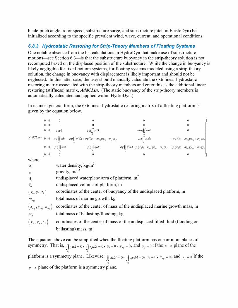
blade-pitch angle, rotor speed, substructure surge, and substructure pitch in ElastoDyn) be initialized according to the specific prevalent wind, wave, current, and operational conditions.

6.8.3 Hydrostatic Restoring for Strip-Theory Members of Floating Systems One notable absence from the list calculations in HydroDyn that make use of substructure motions—see Section 6.3—is that the substructure buoyancy in the strip-theory solution is not recomputed based on the displaced position of the substructure. While the change in buoyancy is likely negligible for fixed-bottom systems, for floating systems modeled using a strip-theory solution, the change in buoyancy with displacement is likely important and should not be neglected. In this latter case, the user should manually calculate the 6x6 linear hydrostatic restoring matrix associated with the strip-theory members and enter this as the additional linear restoring (stiffness) matrix, AddCLin. (The static buoyancy of the strip-theory members is automatically calculated and applied within HydroDyn.)

In its most general form, the 6x6 linear hydrostatic restoring matrix of a floating platform is given by the equation below.

0 0

0 0 0

0 0 0

0

20 0

20 0

0 0 0 0 0 00 0 0 0 0 0

0 0 0

0 0

0 0

0 0 0 0 0

A A

b mg mg f f b mg mg f fA A A

b mg mg f f b mg mg f fA A A

gA g ydA g xdA

AddCLin g ydA g y dA gV z m gz m gz g xydA gV x m gx m gx

g xdA g xydA g x dA gV z m gz m gz gV y m gy m gy

ρ ρ ρ

ρ ρ ρ ρ ρ

ρ ρ ρ ρ ρ

−

= + − − − − + +

− − + − − − + +

∫∫ ∫∫

∫∫ ∫∫ ∫∫

∫∫ ∫∫ ∫∫0

,

where: ρ water density, kg/m3 g gravity, m/s2

0A undisplaced waterplane area of platform, m2

0V undisplaced volume of platform, m3 ( ), ,b b bx y z coordinates of the center of buoyancy of the undisplaced platform, m

mgm total mass of marine growth, kg

( ), ,mg mg mgx y z coordinates of the center of mass of the undisplaced marine growth mass, m

fm total mass of ballasting/flooding, kg

( ), ,f f fx y z coordinates of the center of mass of the undisplaced filled fluid (flooding or ballasting) mass, m

The equation above can be simplified when the floating platform has one or more planes of symmetry. That is,

0

0A

ydA =∫∫ , 0

0A

xydA =∫∫ , 0by = , 0mgy = , and 0fy = if the x z− plane of the

platform is a symmetry plane. Likewise, 0

0A

xdA =∫∫ , 0

0A

xydA =∫∫ , 0bx = , 0mgx = , and 0fx = if the

y z− plane of the platform is a symmetry plane.

The undisplaced coordinates of the center of buoyancy, ( ), ,b b bx y z , center of marine-growth

mass, ( ), ,mg mg mgx y z , and center of filled-fluid mass, ( ), ,f f fx y z , are in the global inertial-frame coordinate system. Most of these parameters can be derived from data found in the HydroDyn summary file. While the equation above makes use of several area integrals, the integrals can often be easily estimated by hand for platforms composed of one or more circular members piercing the waterplane (still-water free surface).

The waterplane area of the undisplaced platform, 0A , affects the hydrostatic load because the displaced volume of the fluid changes with changes in the platform displacement. Similarly, the location of the center of buoyancy of the platform affects the hydrostatic load because its vector position changes with platform displacement and because the cross product of the buoyancy force with the vector position produces hydrostatic moments about the WRP. 0A , 0V , and ( ), ,b b bx y z should be based on the external volume of the platform, including marine-growth thickness. The marine-growth mass and filled-fluid mass also have a direct effect of the hydrostatic restoring because of the moments produced about the WRP.

In classical marine hydrostatics, the effects of body weight are often lumped with the effects of hydrostatics when defining the hydrostatic-restoring matrix; for example, when it is defined in terms of metacentric heights. However, when HydroDyn is coupled to FAST, the body-weight terms (other than the marine-growth and filled-fluid mass within HydroDyn) are automatically accounted for by ElastoDyn, and so, are not included here.

6.8.4 Floating Systems Modeled with Potential Flow Frequency-dependent hydrodynamic coefficients are needed before running the potential-flow solution in HydroDyn. An external pre-processing tool should be used to generate the appropriate frequency-dependent hydrodynamic coefficients. The naming in this manual has focused on WAMIT [Lee, 2006], but other frequency-domain wave-body interaction panel codes can be used that produce similar data. However, in the end, the WAMIT format is what is expected by HydroDyn.

For the first-order potential-flow solution, HydroDyn requires data from the WAMIT files with .1, .3, and .hst extensions. When creating these files, one should keep in mind:

• The .1 file must contain the 6×6 added-mass matrix at infinite frequency (period = zero). Additionally, the .1 file must contain the 6×6 damping matrix over a large range from low frequency to high frequency (the damping should approach zero at both ends of the range). A range of 0.0 to 5.0 rad/s with a discretization of 0.05 rad/s is suggested.

• The .3 file must contain the first-order wave-excitation (diffraction) loads (3 forces and 3 moments) per unit wave amplitude across frequencies and directions where there is wave energy. A range of 0.0 to 5.0 rad/s with a discretization of 0.05 rad/s is suggested and the direction should be specified across the desired range—the full direction range of (-180 to 180] degrees with a discretization of 10 degrees is suggested. While the .3 file contains both the magnitude/phase and real/imaginary components of the first-order wave-excitation loads, only the latter are used by HydroDyn.

• The .hst file should account for the restoring provided by buoyancy, but not the restoring provided by body mass or moorings. (The hydrostatic file is not frequency dependent.) An important thing to keep in mind is that the pitch and roll restoring of a floating body depends on the vertical distance between the center of buoyancy and center of mass of the body. In WAMIT, the vertical center of gravity (VCG) is used to determine the pitch and roll restoring associated with platform weight, and WAMIT will include these effects in the restoring matrix that it outputs (the .hst file). However, the ElastoDyn module of FAST intrinsically accounts for the platform weight’s influence on the pitch and roll restoring if the platform weight and center-of-mass location are defined appropriately. To avoid double booking these terms, it is important to neglect these terms in WAMIT. This can be achieved by setting VCG to zero when solving the first-order problem in WAMIT.

The second-order WAMIT files only need to pre-calculated if a second-order potential-flow option is enabled in HydroDyn. For the second-order mean-drift solution, or for Standing et al.’s extension to Newman’s approximation to the mean- and slow-drift solution, HydroDyn requires WAMIT files with .7, .8. .9, .10d, .11d, or .12d extensions. For the second-order full difference-frequency solution of the mean- and slow-drift terms, HydroDyn requires WAMIT files with .10d, .11d, or .12d extension. For the second-order full sum-frequency solution, HydroDyn requires WAMIT files with .10s, .11s, or .12s extensions. When creating any of these files, one should keep in mind:

• The second-order frequency-domain solution is dependent on first-order body motions, whose accuracy is impacted by properly setting the 6×6 rigid-body mass matrix and center of gravity of the complete floating wind system and the 6×6 mooring system restoring matrix. So, while the body center of gravity and mooring stiffness should be zeroed when creating the first-order WAMIT files, they should not be zeroed when creating the second-order WAMIT files. (Thus, obtaining the first-order and second-order WAMIT files requires distinct WAMIT runs.)

• The .7, .8, and .9 files contain the diagonal of the difference-frequency QTF, based on the first-order potential-flow solution. The files contain the second-order mean-drift loads (3 forces and 3 moments) per unit wave amplitude squared at each first-order wave frequency and pair of wave directions, across a range of frequencies and a range of direction pairs. While the .7, .8, and .9 files contains both the magnitude/phase and real/imaginary components of the second-order wave-excitation loads, only the latter are used by HydroDyn.

• The 10d, .11d, and .12d, or .10s, .11s, and .12s files contain the full difference- and sum-frequency QTFs, respectively, based on the first-order or first- plus second-order potential-flow solutions. The files contain the second-order wave-excitation (diffraction) loads (3 forces and 3 moments) per unit wave amplitude squared at each pair of first-order wave frequencies and directions, across a range of frequency and direction pairs. While the 10d, .11d,.12d, .10s, .11s, and .12s files contains both the magnitude/phase and real/imaginary components of the second-order wave-excitation loads, only the latter are used by HydroDyn.

• The frequencies and directions in the WAMIT files do not need to be evenly spaced.

• The discretization of the first set of directions does not need to be the same as the discretization of the second set of directions; however, the matrix of direction pairs must be fully populated (not sparse). Both sets of directions should span across the desired range—the full direction range of (-180 to 180] degrees with a discretization of 10 degrees is suggested.

• The frequencies should span the range where there is first-order wave energy and the frequency discretization should be such that the differences and sums between pairs of frequencies span the range where there is second-order wave energy. A range of 0.25 to 2.75 rad/s with a discretization of 0.05 rad/s is suggested.

• Second-order hydrodynamic theory dictates that difference-frequency QTFs are conjugate symmetric between frequency pairs and sum-frequency QTFs are symmetric between frequency pairs. Due to this symmetry, the QTFs (the 10d, .11d, or .12d, .10s, .11s, and .12s files) may be upper triangular, lower triangular, a mix of upper and lower triangular terms, or full; however, after applying the symmetry, the matrix of frequency pairs must be fully populated (not sparse). When an element of the QTF is supplied together with its symmetric pairing, HydroDyn will warn the user if the QTF is not properly symmetric.

7 HydroDyn Theory This is a preliminary draft of the HydroDyn theory and should be considered a work in progress.

Hydrodynamics are modeled using a suitable combination of incident-wave kinematics and hydrodynamic loading models. Hydrodynamic loads result from the integration of the dynamic pressure of the water over the wetted surface of a floating platform. These loads include contributions from inertia (added mass) and linear drag (radiation), buoyancy (restoring), incident-wave scattering (diffraction), sea current, and nonlinear effects.

7.1 Coordinate Systems

7.1.1 Global coordinate system: ( ), ,X Y Z

• The global axes are represented by the unit vectors I , J , and K . • The origin is set at the mean sea level, the center of the structure, with 𝑍 axis positive

upward. • The positive 𝑋 axis is along the nominal (zero-degree) wave propagation direction. • The Y axis can be found assuming a right-handed Cartesian coordinate system.

7.1.2 Structural member local coordinate system: ( ), ,x y z

• Axes are represented by the unit vectors i , j , and k . • The origin is set at the center of the structural member. • The local 𝑧 axis is along the cylinder axis, directed from the start joint to the end joint.

The start joint is defined as the joint that has a lower 𝑍 coordinate value. If the two joints have the same 𝑍 coordinate value, then the one that has the lower 𝑋 coordinate value is the start point. If the two joints have the same 𝑍 and 𝑋 coordinate value, then the one that has the lower 𝑌 coordinate value is the start point.

• The local 𝑥 axis is parallel to the global 𝑋𝑍 plane, positive along the nominal wave propagation direction. If the cylinder’s axis is along the global 𝑋 direction, then the local 𝑥 axis is parallel to the 𝑋𝑍 plane, and positive along the negative global 𝑍 direction.

• The local y axis can be found assuming a right-handed Cartesian coordinate system.

7.1.3 Local to Global transformation For regular members, the cylinder expression in global coordinate system can be found as follows:

[ ]2cos

sin2

2

s e

s e

s e

X X

X rY YY r

Z z Z Z

θθ

+

+ = +

+

C

where ( ), ,s s sX Y Z and ( ), ,e e eX Y Z are the start and end joints of the member in global

coordinate system of the member, and [ ]C is the direction cosine matrix of the member axis and can be obtained as follows:

[ ]

( )( )

( )( )

0

e s e se s e s

xz xz

xz e s

e s e se s e s

xz xz

X X Y YZ Z X XL L L L

L Y YL L

Z Z Y YX X Z ZL L L L

− − − −−

−

= − −− + −

−

C

where ( ) ( )2 2xz e s e sL X X Z Z= − + − and ( ) ( ) ( )2 2 2

e s e s e sL X X Y Y Z Z= − + − + − . When

e sX X= and e sZ Z= , the [ ]C matrix can be found as follows: if e sY Y< e sY Y< then

[ ]1 0 00 0 10 1 0

= −

C

else

[ ]1 0 00 0 10 1 0

= −

C

7.2 Wave Kinematics The wave kinematics are modeled using Airy wave theory, which can be used to describe either regular or irregular waves. For regular waves, the wave elevation (ζ) is represented as a sinusoid with a single amplitude (wave height) and frequency. Airy wave theory also describes how the undisturbed fluid-particle velocities and accelerations decay exponentially with depth. Irregular or random waves can then be represented as a summation or superposition of multiple wave components, as described by an appropriate wave spectrum:

( ) 21 ( ) 2 ( )2

sided j tt W S e dωζζ ω π ω ω

π

∞−

−∞

= ∫

This equation represents the wave elevation as an inverse Fourier transform of the desired two-sided power spectral density, 2 sidedSζ

− where j is an imaginary number and ω is an individual wave frequency. W(ω) is the Fourier transform of a realization of a white Gaussian noise (WGN) time-series process with zero mean and unit variance (i.e., the so-called “standard normal distribution”). This realization is used to ensure that the individual wave components have a random phase and that the instantaneous wave elevation is normally- (i.e., Gaussian-)

distributed with zero mean and with a variance, on average, equal to ( )2 2-Sided

-

S dζ ζσ ω ω∞

∞

= ∫ .

Further details about the wave kinematics and how they are computed can be found in [Jonkman, 2007].

7.3 Current Model The current model within HydroDyn is a superposition of three different types of sub-models These sub-models follow the forms defined in the IEC 61400-3 offshore wind standard [IEC, 2009].

The first is a sub-surface current model for currents that are generated by tides, storm surge, atmospheric pressure variations, etc. This model is characterized by a simple 1/7 power law over the water depth, d.

( )17

0SSSSZ dU Z U

d+ =

The second is near-surface currents generated by wind. This model is characterized by a linear

distribution of the velocity with water depth, ending at zero at a prescribed depth, refh (in [IEC,

2009], refh is set at 20 m).

( ) 0 , ,0NS

refNS ref

ref

Z hU Z U Z h

h +

= ∈ − otherwise, ( ) 0NSU Z =

The third model is a depth-independent model, which sets the current velocity to a constant value across the water depth.

You can specify a unique heading direction for each of the three current models.

7.4 Potential Flow Theory Three main approaches exist for modeling the hydrodynamic loads within HydroDyn, potential-flow theory, strip theory (via Morison’s equation), or a combination. This section reviews the forces modeled in HydroDyn when using a linear potential flow theory approach.

7.4.1 Modeling Approach In linear potential-flow theory, the forces and added mass are applied at the platform reference point. The components are:

nWRP W HS RD AMF F F F F= + + +

where

AM PRPF AM a= −

[ ] ( ) ( )22

2

12

1 2 ,

NknjSided NW

kNk

F W k S X eN t

π

ζ ω ω

π ω ω β−

= ∆=− −

=∆∑

{ } { } { }( )0 3 4 5CB CB Hydrostatic

HSF gV y x C xρ δ δ δ= + − −

The general form of the convolution integral is:

( ) ( )0

t

RDF K t x dτ τ τ= − − ⋅∫

But we discretize this and only consider a specific amount time history, RDN :

1

1n

RD

n

RD RD n i ii n N

F t K x−

− −= −

= −∆ ∑

The state for time step n is simply the structural velocities for the previous RDN time steps. Or,

1

2

RD

n

ndn

n N

xx

x

x

−

−

−

=

Therefore, at time step n, we can compute the n+1 state, such that,

11

1RD

n

ndn

n N

xx

x

x

−+

− +

=

The radiation step size, RDt∆ , and the radiation kernel, K , are simply module parameters.

7.5 Morison’s Equation Morison’s equation is applicable for calculating the hydrodynamic loads on cylindrical structures when (1) the effects of diffraction are negligible, (2), radiation damping is negligible, and (3) flow separation may occur. The relative form of Morison’s equation accounts for wave loading from incident-wave-induced excitation, radiation-induced added mass, and flow-separation-induced viscous drag. In this section we review the representation of Morison’s equation both when considering distributed forces along the length of the members (at nodes) and point loads at the ends (at the joints).

7.5.1 Modeling Approach In the present version of HydroDyn, Morison forces are applied only along the portion of the member below the SWL. Wave stretching theory has not yet been implemented. In addition, the forces are applied at the original position of the structure, and not at the instantaneous position.

7.5.1.1 Distributed Loads For a Morison-only model, the distributed hydrodynamic loads applied along the length of a member are computed as:

_ _ _ _I D B MG F B AM M AM MG AM FF F F F F F F F F= + + + + + + +

where FI is the inertia force, FD the drag force, FB the buoyancy force, FMG the weight of the marine growth, FF_B the force due to fluid ballasting, FAM_M the added mass of the structure, FAM_MG the added mass due to marine growth, and FAM_F the added mass due to fluid ballasting. Details about each of these forces will be provided in the following sections. All of these forces except the buoyancy forces, BF

, and _F BF

, are applied directly to a mesh node.

If a hybrid model is desired, which combines contributions from both potential-flow theory and Morison’s equation, the only components that are considered for Morison’s equation are:

_ _D F B AM FF F F F= + +

7.5.1.1.1 Inertial Loads The inertial force component of Morison’s equation is associated with the fluid acceleration, and includes two terms. The first is the Froude-Krylov term associated with the unsteady pressure field generated by the undisturbed waves. This term can be controlled using the CP coefficient, with a value of 1.0 being the default. The second term is the scattering force associated with the disruption of the fluid by the presence of the structure. This term is controlled by the coefficient of added mass, CA. The equation below gives the full representation of the inertia force, which includes transverse and axial forces (represented by the Ax subscript).

( ) ( ) ( ) ( ) ( ) ( ) ( ) 2 22 2

000

Ax Axf f fP A W MG P MG dyn A W MG

I

R RC C R t a a k k C R t p C R t a k kz z

F

ρ π π ρ π ∂ ∂

+ + − • + + + + • ∂ ∂ =

where ( ) ( )

( )e e s s

mg mg

e s

R t R tRz Z Z

+ − +∂=

∂ −

It is noted that P A MC C C+ = , the inertia coefficient. CP is called the dynamic pressure coefficient. By creating the dynamic pressure coefficient, CM and CA can be controlled independently.

7.5.1.1.2 Viscous Drag The second major component of Morison’s equation is the viscous drag force, which is represented in the equation below. The viscous drag force is proportional to the square of relative velocity between the fluid and the structure, and is scaled using the coefficient of drag, CD.

( ) ( ) ( ) ( )2

000

rel rel rel relD W MG

D

C R t v v k k v v k k

F

ρ + − • − •

=

7.5.1.1.3 Buoyancy The next term presented is the buoyancy term, which is the force directed along the global Z-axis equal to the weight of the displaced fluid when the platform is in its undisplaced position.

( )( )

( )

( )

( )

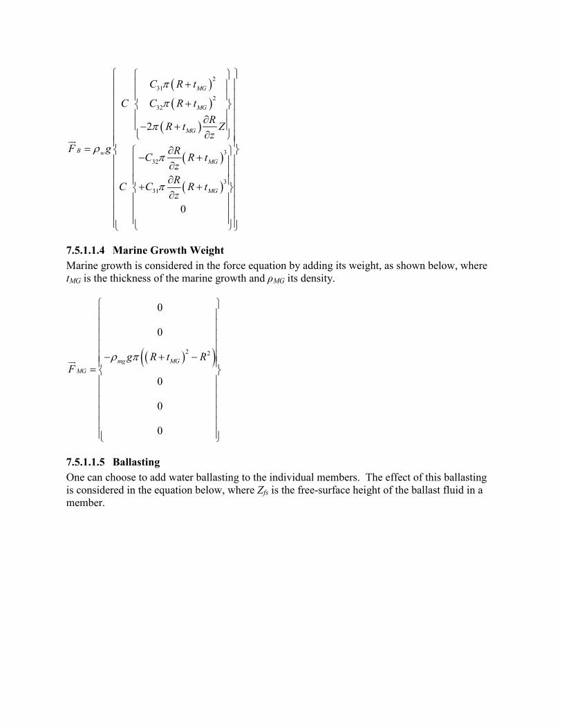
31

32

323

331

2

2

2

0

MG

MG

MG

wMG

B

MG

R t

R t

R t

gR t

R

C

C CR Zz

F RCzRC Cz

t

π

π

π

ρπ

π

+

+

− +

∂

∂ +

= ∂−

∂+

∂

+∂

7.5.1.1.4 Marine Growth Weight Marine growth is considered in the force equation by adding its weight, as shown below, where tMG is the thickness of the marine growth and ρMG its density.

( )( )2 2

0

0

0

0

0

mg MGMG

g R t RF

ρ π

− + − =

7.5.1.1.5 Ballasting One can choose to add water ballasting to the individual members. The effect of this ballasting is considered in the equation below, where Zfs is the free-surface height of the ballast fluid in a member.

( )( )

( ) ( )

( )

( )

2

2

3

3

31

32

_

32

31

2

0

f

fs

F B

C

C CR Z

R t

R t

R t

gR t

Zz

F RCz

RC C R tz

π

ρ

π

π

π

π

−

−

− − −

∂

−

−∂

= − ∂−

∂

∂

∂

7.5.1.1.6 Hydrodynamic Added Mass The next group of terms is associated with the added mass of the structure, which is proportional to the acceleration of the structure. The added mass is the inertia added to a system because an accelerating body must move some volume of surrounding fluid as it moves through it. In the equations below, both transverse and axial terms are shown.

( ) ( ) [ ]

[ ] [ ]

2 2 0

0 0

Ax

T T

A AM W MG

RC I kk C kkzAM R tρ π

∂ − − ∂= +

_s

AM M Ms

aF AM

α

= −

7.5.1.1.7 Added Mass due to Marine Growth If marine growth is applied to the structure, this additional volume will alter the added mass calculation. Here, the influence of the marine growth is captured through an additional term.

( )( )2 2

1 0 0 0 0 00 1 0 0 0 00 0 1 0 0 00 0 0 0 0 00 0 0 0 0 00 0 0 0 0 0

MG mg MGAM R t Rρ π

= + −

_s

AM MG MGs

aF AM

α

= −

7.5.1.1.8 Added Mass due to Ballasting Similarly, the added mass is altered by the existence of fluid ballasting, which is captured in the following equations.

( )2

1 0 0 0 0 00 1 0 0 0 00 0 1 0 0 00 0 0 0 0 00 0 0 0 0 00 0 0 0 0 0

F f MAM R tρ π

= −

_s

AM F Fs

aF AM

α

= −

7.5.1.2 Lumped Loads at member ends The previous section covered distributed forces along the length of a member. Now, lumped forces at member ends are considered.

When using a Morison-only model, the lumped forces for Morison’s equation at the member ends include the following components:

_I D B F B AMF F F F F F= + + + +

However, if the member is modeled using a hybrid approach combining both potential flow theory and Morison’s equation, only the following terms are considered:

_D F BF F F= +

The influences of the individual terms in Morison’s equation in a lumped formulation are the same as the description for the distributed forces, but the implementation changes. Whereas the distributed forces considered the projected area and diameter of the member assuming a cylindrical geometry, at the ends the member is considered a flat plate in Morison’s equation.

7.5.1.2.1 Inertial Loads

( )

( )( )2

00

000

Ax

Ax

fA W n ns

n ns ssP MG dynI

C V a VC

V VC R t pF

ρ

π

• + • + =

(32)

( )

( )( )2

00

000

Ax

Ax

fA W n ne

n ne eeP MG dynI

C V a VC

V VC R t pF

ρ

π

• − + • + =

(33)

where ( )32 ˆ3

Mi

n MGi ii

V R t nπ= +∑

The terms in sIF

and eIF

involving AxAC must be divided by M and distributed equally to the

start/end node each member at each joint.

7.5.1.2.2 Viscous Drag

( )( )

2

ˆ

4

000

Ax

M

n i ii

rel relD W n n n

n n

D

A A n

C A v A v A

A AF

ρ

=

• • • =

∑

(31)

Equation 31 is the total lumped drag at a joint, since the simulation mesh consists of M co-

located lumped nodes, DF

is actually DFM

, for each simulation node.

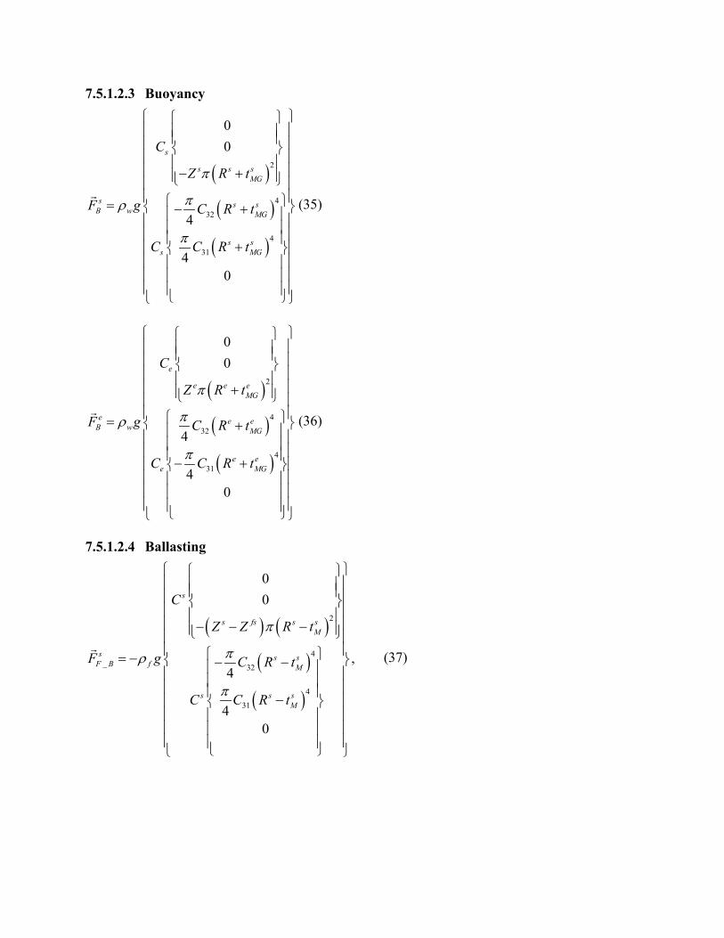
7.5.1.2.3 Buoyancy

( )

( )

( )

4

32

4

31

2

40

00

4

s s sMG

s sw MG

s sM

s

sB

s G

C

F C

C

Z R t

g R t

R tC

π

π

ρ

π

− +

+

+

= −

(35)

( )

( )

( )

4

32

4

31

2

00

4

40

e e eMG

e ew MG

e eM

e

G

e

B

e

C

F C

C

Z

tC

R t

g R t

R

π

ρ π

π

+

+

+

= −

(36)

7.5.1.2.4 Ballasting

( ) ( )

( )

( )

4_ 32

4

3

2

1

00

,

40

4

s fs s sM

s sf M

s

sF

sM

s

B

s

Z Z R t

g R t

C

F C

C C R t

π

ρ π

π

= − −

− − −

−

−

(37)

( ) ( )

( )

( )

4_ 32

3

2

4

1

00

4

40

e fs e eM

e ef M

e eM

e

eF B

e

C

F C

C C

Z Z R t

g R t

R t

π

ρ π

π

− −

−

−

= − −

7.5.1.2.5 Hydrodynamic Added Mass

( )( )

000

AxsA W n n

n n

AM

C V a V

V VF

ρ − • •

=

This is the total lumped added mass force at a joint, since the simulation mesh consists of M co-

located lumped nodes, AMF

is actually AMFM

, for each simulation node.

Note that ˆin is the outward facing normal vector, so, ˆ iin k= − at the start (s) of a member and ˆ iin k= at the end (e) of a member.

7.5.2 Simulation Discretization HydroDyn refines the input geometry of joints and members into a resulting set of nodes and elements using the following algorithm:

1. Copy initial input geometry of joints/members to an initial node/element description.

2. For each element, swap the element nodes if they do not satisfy the specifications of Section 7.1.2.

3. For each element, determine if the element needs to be split for any of the following reasons; adding a node and an element to the mesh for each positive test:

o The element is filled and the free-surface elevation lies within the element; add node at free-surface elevation.

o The element crosses the MSL2SWL elevation; add node at MSL2SWL elevation.

o The element crosses the seabed; add node at seabed elevation.

o The element crosses the upper and/or lower marine-growth elevations; add one or two nodes corresponding to the upper and/or lower marine growth elevations.

4. For each resulting element, if its length is greater than MDivSize for its associated input member, then subdivide into the necessary number of additional elements such that each element’s length is less than or equal to MDivSize. Any new nodes created as a part of this subdivision are referred to as “interior nodes”.

5. Finally, for each non-interior node, determine if it connects to more than one element. If so, make N-1 copies of that node, where N is the number of elements connecting to the node. Redefine the connectivity of these connected elements such that the original node and the new nodes connect to only one element.

8 Future Work This list contains features that we will implement in future releases:

• Enable times-series input motions for Morison members in the standalone HydroDyn (MorisonInputsMod = 2)

• Enable tight-coupling to FAST, including linearization.

• Enable wave stretching (WaveStMod > 0).

• Enable full support for floating platform force flags.

• Enable joint overlap calculations (JointOvrlp = 1).

• Support for user-defined wave time history.

• Enable auto-generation of all possible output channels (OutAll = TRUE).

• Ensure that the output channels are written in the order they are entered.

• Allow for a WAMIT reference point location other than (0,0,0).

• Allow RdtnDT to be independent from the FAST simulation time step

• Add distributed axial viscous-drag loads on tapered members.

• Add rotational inertia terms for fluid-filled members and marine growth.

• Calculate the effective 6x6 added-mass matrix from strip-theory members and place in the HydroDyn summary file.

• Add graphics/animation capability to visualize the substructure geometry and motion, wave elevation, and hydrodynamic loads.

• Further validation with test data.

• Add higher order regular wave kinematics models for fixed-bottom substructures.

• Add breaking wave-impact loads for fixed-bottom substructures.

• Add floating platform hydro-elastics.

• Add pressure mapping for floating platforms.

• Fix the problem whereby HydroDyn can’t be run after compiling with gFortran.

• Added automated computation and use of hydrostatic restoring matrix for strip-theory members.

9 References This is a preliminary draft of the reference list and should be considered a work in progress.

IEC 61400-3 Ed.1, Wind Turbines – Part 3: Design Requirements for Offshore Wind Turbines, International Electrotechnical Commission (IEC), 2009.

Jonkman, J. M., Dynamic modeling and load analysis of an offshore floating wind turbine, Ph.D. Thesis. Department of Aerospace Engineering Sciences, University of Colorado, Boulder, CO, 2007; NREL/TP-500-41958. Golden, CO: National Renewable Energy Laboratory.

Lee, C. H. and Newman, J. N., WAMIT® User Manual, Versions 6.3, 6.3PC, 6.3S, 6.3S-PC, Chestnut Hill, MA: WAMIT, Inc., 2006.

Sharma, N. and Dean. R., “Second-order directional seas and associated wave forces,” Society of Petroleum Engineers Journal, 4:129-140, 1981.

Appendix A. OC4 Semi-submersible Input File ------- HydroDyn v2.01.* Input File -------------------------------------------- NREL 5.0 MW offshore baseline floating platform HydroDyn input properties for the OC4 Semi-submersible. False Echo - Echo the input file data (flag) ---------------------- ENVIRONMENTAL CONDITIONS -------------------------------- 1025 WtrDens - Water density (kg/m^3) 200 WtrDpth - Water depth (meters) 0 MSL2SWL - Offset between still-water level and mean sea level (meters) [positive upward; must be zero if HasWAMIT=TRUE] ---------------------- WAVES --------------------------------------------------- 3 WaveMod - Incident wave kinematics model {0: none=still water, 1: plane progressive (regular), 1P#: plane progressive with user-specified phase, 2: … 0 WaveStMod - Model for stretching incident wave kinematics to instantaneous free surface {0: none=no stretching, 1: vertical stretching, 2: extrapolation … 4600 WaveTMax - Analysis time for incident wave calculations (sec) [unused when WaveMod=0] [determines WaveDOmega=2Pi/WaveTMax in the IFFT] 0.2 WaveDT - Time step for incident wave calculations (sec) [unused when WaveMod=0] [0.1<=WaveDT<=1.0 recommended] [determines WaveOmegaMax=Pi/WaveDT in the IFFT] 1.2646 WaveHs - Significant wave height of incident waves (meters) [used only when WaveMod=1, 2, or 3] 10 WaveTp - Peak-spectral period of incident waves (sec) [used only when WaveMod=1 or 2] "DEFAULT" WavePkShp - Peak-shape parameter of incident wave spectrum (-) or DEFAULT (string) [used only when WaveMod=2] [use 1.0 for Pierson-Moskowitz] 0.314159 WvLowCOff - Low cut-off frequency or lower frequency limit of the wave spectrum beyond which the wave spectrum is zeroed (rad/s) [used only when WaveMod=2, 3, or 4] 1.570796 WvHiCOff - High cut-off frequency or upper frequency limit of the wave spectrum beyond which the wave spectrum is zeroed (rad/s) [used only when WaveMod=2, 3, or 4] 0 WaveDir - Incident wave propagation heading direction (degrees) [unused when WaveMod=0 or 5] 0 WaveDirMod - Directional spreading function {0: none, 1: COS2S} (-) [only used when WaveMod=2,3,4] 1 WaveDirSpread - Wave direction spreading coefficient ( > 0 ) (-) [only used when WaveMod=2,3,4 and WaveDirMod=1] 1 WaveNDir - Number of wave directions (-) [odd number only, may be adjusted within HydroDyn] 0 WaveDirRange - Range of wave directions (full range: WaveDir +/- 1/2*WaveDirRange) (degrees) [only used when WaveMod=2,3,4 and WaveDirMod=1] 123456789 WaveSeed(1) - First random seed of incident waves [-2147483648 to 2147483647] (-) [unused when WaveMod=0 or 5] 1011121314 WaveSeed(2) - Second random seed of incident waves [-2147483648 to 2147483647] (-) [unused when WaveMod=0 or 5] FALSE WaveNDAmp - Flag for normally distributed amplitudes (flag) "" GHWvFile - Root name of GH Bladed files containing wave data (quoted string) [used only when WaveMod=5] 1 NWaveElev - Number of points where the incident wave elevations can be computed (-) [maximum of 9 output locations] 0 WaveElevxi - List of xi-coordinates for points where the incident wave elevations can be output (meters) [NWaveElev points, separated by commas or white space; … 0 WaveElevyi - List of yi-coordinates for points where the incident wave elevations can be output (meters) [NWaveElev points, separated by commas or white space; … ---------------------- 2ND-ORDER WAVES ----------------------------------------- False WvDiffQTF - Full difference-frequency 2nd-order wave kinematics (flag) False WvSumQTF - Full summation-frequency 2nd-order wave kinematics (flag) 0 WvLowCOffD - Low frequency cutoff used in the difference-frequencies (rad/s) [Only used with a difference-frequency method] 500 WvHiCOffD - High frequency cutoff used in the difference-frequencies (rad/s) [Only used with a difference-frequency method] 0 WvLowCOffS - Low frequency cutoff used in the summation-frequencies (rad/s) [Only used with a summation-frequency method] 500 WvHiCOffS - High frequency cutoff used in the summation-frequencies (rad/s) [Only used with a summation-frequency method] ---------------------- CURRENT ------------------------------------------------- 0 CurrMod - Current profile model {0: none=no current, 1: standard, 2: user-defined from routine UserCurrent} (switch) 0 CurrSSV0 - Sub-surface current velocity at still water level (m/s) [used only when CurrMod=1] "DEFAULT" CurrSSDir - Sub-surface current heading direction (degrees) or DEFAULT (string) [used only when CurrMod=1] 20 CurrNSRef - Near-surface current reference depth (meters) [used only when CurrMod=1] 0 CurrNSV0 - Near-surface current velocity at still water level (m/s) [used only when CurrMod=1] 0 CurrNSDir - Near-surface current heading direction (degrees) [used only when CurrMod=1] 0 CurrDIV - Depth-independent current velocity (m/s) [used only when CurrMod=1] 0 CurrDIDir - Depth-independent current heading direction (degrees) [used only when CurrMod=1] ---------------------- FLOATING PLATFORM --------------------------------------- TRUE HasWAMIT - Using WAMIT (flag) "HydroData/marin_semi" WAMITFile - Root name of WAMIT output files containing the linear, nondimensionalized, hydrostatic restoring matrix (.hst extension), … 1 WAMITULEN - Characteristic body length scale used to redimensionalize WAMIT output (meters) 13917 PtfmVol0 - Displaced volume of water when the platform is in its undisplaced position (m^3) [USE THE SAME VALUE COMPUTED BY WAMIT AS OUTPUT IN THE .OUT FILE!] 0 PtfmCOBxt - The xt offset of the center of buoyancy (COB) from the platform reference point (meters) 0 PtfmCOByt - The yt offset of the center of buoyancy (COB) from the platform reference point (meters) 1 RdtnMod - Radiation memory-effect model {0: no memory-effect calculation, 1: convolution, 2: state-space} (switch) [STATE-SPACE REQUIRES *.ss INPUT FILE]

60 RdtnTMax - Analysis time for wave radiation kernel calculations (sec) [determines RdtnDOmega=Pi/RdtnTMax in the cosine transform] [MAKE SURE THIS … 0.0125 RdtnDT - Time step for wave radiation kernel calculations (sec) [DT<=RdtnDT<=0.1 recommended] [determines RdtnOmegaMax=Pi/RdtnDT in the cosine transform] ---------------------- 2ND-ORDER FLOATING PLATFORM FORCES ---------------------- 0 MnDrift - Mean-drift 2nd-order forces computed {0: None; [7, 8, 9, 10, 11, or 12]: WAMIT file to use} [Only one of … 0 NewmanApp - Mean- and slow-drift 2nd-order forces computed with Newman's approximation {0: None; [7, 8, 9, 10, 11, or 12]: WAMIT file to use} [Only one of … 0 DiffQTF - Full difference-frequency 2nd-order forces computed with full QTF {0: None; [10, 11, or 12]: WAMIT file to use} [Only one of … 0 SumQTF - Full summation -frequency 2nd-order forces computed with full QTF {0: None; [10, 11, or 12]: WAMIT file to use} ---------------------- FLOATING PLATFORM FORCE FLAGS -------------------------- True PtfmSgF - Platform horizontal surge translation force (flag) or DEFAULT True PtfmSwF - Platform horizontal sway translation force (flag) or DEFAULT True PtfmHvF - Platform vertical heave translation force (flag) or DEFAULT True PtfmRF - Platform roll tilt rotation force (flag) or DEFAULT True PtfmPF - Platform pitch tilt rotation force (flag) or DEFAULT True PtfmYF - Platform yaw rotation force (flag) or DEFAULT ---------------------- PLATFORM ADDITIONAL STIFFNESS AND DAMPING -------------- 0 0 0 0 0 0 AddF0 - Additional preload (N, N-m) 0 0 0 0 0 0 AddCLin - Additional linear stiffness (N/m, N/rad, N-m/m, N-m/rad) 0 0 0 0 0 0 0 0 0 0 0 0 0 0 0 1451298897 0 0 0 0 0 0 1451298897 0 0 0 0 0 0 0 0 0 0 0 0 0 AddBLin - Additional linear damping(N/(m/s), N/(rad/s), N-m/(m/s), N-m/(rad/s)) 0 0 0 0 0 0 0 0 0 0 0 0 0 0 0 0 0 0 0 0 0 0 0 0 0 0 0 0 0 0 0 0 0 0 0 0 AddBQuad - Additional quadratic drag(N/(m/s)^2, N/(rad/s)^2, N-m(m/s)^2, N-m/(rad/s)^2) 0 0 0 0 0 0 0 0 0 0 0 0 0 0 0 0 0 0 0 0 0 0 0 0 0 0 0 0 0 0 ---------------------- AXIAL COEFFICIENTS -------------------------------------- 2 NAxCoef - Number of axial coefficients (-) AxCoefID AxCd AxCa AxCp (-) (-) (-) (-) 1 0.00 0.00 1.00 2 9.60 0.00 1.00 ---------------------- MEMBER JOINTS ------------------------------------------- 44 NJoints - Number of joints (-) [must be exactly 0 or at least 2] JointID Jointxi Jointyi Jointzi JointAxID JointOvrlp [JointOvrlp= 0: do nothing at joint, 1: eliminate overlaps by calculating super member] (-) (m) (m) (m) (-) (switch) 1 0.00000 0.00000 -20.00000 1 0 2 0.00000 0.00000 10.00000 1 0 3 14.43376 25.00000 -14.00000 1 0 4 14.43376 25.00000 12.00000 1 0 5 -28.86751 0.00000 -14.00000 1 0 6 -28.86751 0.00000 12.00000 1 0 7 14.43376 -25.00000 -14.00000 1 0 8 14.43376 -25.00000 12.00000 1 0 9 14.43375 25.00000 -20.00000 2 0 10 -28.86750 0.00000 -20.00000 2 0 11 14.43375 -25.00000 -20.00000 2 0 12 9.23760 22.00000 10.00000 1 0 13 -23.67130 3.00000 10.00000 1 0

14 -23.67130 -3.00000 10.00000 1 0 15 9.23760 -22.00000 10.00000 1 0 16 14.43375 -19.00000 10.00000 1 0 17 14.43375 19.00000 10.00000 1 0 18 4.04145 19.00000 -17.00000 1 0 19 -18.47520 6.00000 -17.00000 1 0 20 -18.47520 -6.00000 -17.00000 1 0 21 4.04145 -19.00000 -17.00000 1 0 22 14.43375 -13.00000 -17.00000 1 0 23 14.43375 13.00000 -17.00000 1 0 24 1.62500 2.81500 10.00000 1 0 25 11.43376 19.80385 10.00000 1 0 26 -3.25000 0.00000 10.00000 1 0 27 -22.87000 0.00000 10.00000 1 0 28 1.62500 -2.81500 10.00000 1 0 29 11.43376 -19.80385 10.00000 1 0 30 1.62500 2.81500 -17.00000 1 0 31 8.43376 14.60770 -17.00000 1 0 32 -3.25000 0.00000 -17.00000 1 0 33 -16.87000 0.00000 -17.00000 1 0 34 1.62500 -2.81500 -17.00000 1 0 35 8.43376 -14.60770 -17.00000 1 0 36 1.62500 2.81500 -16.20000 1 0 37 11.43376 19.80385 9.13000 1 0 38 -3.25000 0.00000 -16.20000 1 0 39 -22.87000 0.00000 9.13000 1 0 40 1.62500 -2.81500 -16.20000 1 0 41 11.43376 -19.80385 9.13000 1 0 42 14.43376 25.00000 -19.94000 1 0 43 -28.86751 0.00000 -19.94000 1 0 44 14.43376 -25.00000 -19.94000 1 0 ---------------------- MEMBER CROSS-SECTION PROPERTIES ------------------------- 4 NPropSets - Number of member property sets (-) PropSetID PropD PropThck (-) (m) (m) 1 6.50000 0.03000 ! Main Column 2 12.00000 0.06000 ! Upper Columns 3 24.00000 0.06000 ! Base Columns 4 1.60000 0.01750 ! Pontoons ---------------------- SIMPLE HYDRODYNAMIC COEFFICIENTS (model 1) -------------- SimplCd SimplCdMG SimplCa SimplCaMG SimplCp SimplCpMG SimplAxCa SimplAxCaMG SimplAxCp SimplAxCpMG (-) (-) (-) (-) (-) (-) (-) (-) (-) (-) 0.00 0.00 0.00 0.00 1.00 1.00 0.00 0.00 1.00 1.00 ---------------------- DEPTH-BASED HYDRODYNAMIC COEFFICIENTS (model 2) --------- 0 NCoefDpth - Number of depth-dependent coefficients (-) Dpth DpthCd DpthCdMG DpthCa DpthCaMG DpthCp DpthCpMG DpthAxCa DpthAxCaMG DpthAxCp DpthAxCpMG (m) (-) (-) (-) (-) (-) (-) (-) (-) (-) (-) ---------------------- MEMBER-BASED HYDRODYNAMIC COEFFICIENTS (model 3) -------- 25 NCoefMembers - Number of member-based coefficients (-) MemberID MemberCd1 MemberCd2 MemberCdMG1 MemberCdMG2 MemberCa1 MemberCa2 MemberCaMG1 MemberCaMG2 MemberCp1 MemberCp2 MemberCpMG1 MemberCpMG2 … (-) (-) (-) (-) (-) (-) (-) (-) (-) (-) (-) (-) (-) … 1 0.56 0.56 0.00 0.00 0.00 0.00 0.00 0.00 0.00 0.00 0.00 0.00 … 2 0.61 0.61 0.00 0.00 0.00 0.00 0.00 0.00 0.00 0.00 0.00 0.00 … 3 0.61 0.61 0.00 0.00 0.00 0.00 0.00 0.00 0.00 0.00 0.00 0.00 … 4 0.61 0.61 0.00 0.00 0.00 0.00 0.00 0.00 0.00 0.00 0.00 0.00 … 5 0.68 0.68 0.00 0.00 0.00 0.00 0.00 0.00 0.00 0.00 0.00 0.00 …

6 0.68 0.68 0.00 0.00 0.00 0.00 0.00 0.00 0.00 0.00 0.00 0.00 … 7 0.68 0.68 0.00 0.00 0.00 0.00 0.00 0.00 0.00 0.00 0.00 0.00 … 23 0.68 0.68 0.00 0.00 0.00 0.00 0.00 0.00 0.00 0.00 0.00 0.00 … 24 0.68 0.68 0.00 0.00 0.00 0.00 0.00 0.00 0.00 0.00 0.00 0.00 … 25 0.68 0.68 0.00 0.00 0.00 0.00 0.00 0.00 0.00 0.00 0.00 0.00 … 8 0.63 0.63 0.00 0.00 0.00 0.00 0.00 0.00 0.00 0.00 0.00 0.00 … 9 0.63 0.63 0.00 0.00 0.00 0.00 0.00 0.00 0.00 0.00 0.00 0.00 … 10 0.63 0.63 0.00 0.00 0.00 0.00 0.00 0.00 0.00 0.00 0.00 0.00 … 11 0.63 0.63 0.00 0.00 0.00 0.00 0.00 0.00 0.00 0.00 0.00 0.00 … 12 0.63 0.63 0.00 0.00 0.00 0.00 0.00 0.00 0.00 0.00 0.00 0.00 … 13 0.63 0.63 0.00 0.00 0.00 0.00 0.00 0.00 0.00 0.00 0.00 0.00 … 14 0.63 0.63 0.00 0.00 0.00 0.00 0.00 0.00 0.00 0.00 0.00 0.00 … 15 0.63 0.63 0.00 0.00 0.00 0.00 0.00 0.00 0.00 0.00 0.00 0.00 … 16 0.63 0.63 0.00 0.00 0.00 0.00 0.00 0.00 0.00 0.00 0.00 0.00 … 17 0.63 0.63 0.00 0.00 0.00 0.00 0.00 0.00 0.00 0.00 0.00 0.00 … 18 0.63 0.63 0.00 0.00 0.00 0.00 0.00 0.00 0.00 0.00 0.00 0.00 … 19 0.63 0.63 0.00 0.00 0.00 0.00 0.00 0.00 0.00 0.00 0.00 0.00 … 20 0.63 0.63 0.00 0.00 0.00 0.00 0.00 0.00 0.00 0.00 0.00 0.00 … 21 0.63 0.63 0.00 0.00 0.00 0.00 0.00 0.00 0.00 0.00 0.00 0.00 … 22 0.63 0.63 0.00 0.00 0.00 0.00 0.00 0.00 0.00 0.00 0.00 0.00 … -------------------- MEMBERS ------------------------------------------------- 25 NMembers - Number of members (-) MemberID MJointID1 MJointID2 MPropSetID1 MPropSetID2 MDivSize MCoefMod PropWAMIT [MCoefMod=1: use simple coeff table, 2: use depth-based coeff table, 3: use member-based … (-) (-) (-) (-) (-) (m) (switch) (flag) 1 1 2 1 1 1.0000 3 TRUE ! Main Column 2 3 4 2 2 1.0000 3 TRUE ! Upper Column 1 3 5 6 2 2 1.0000 3 TRUE ! Upper Column 2 4 7 8 2 2 1.0000 3 TRUE ! Upper Column 3 5 42 3 3 3 1.0000 3 TRUE ! Base Column 1 6 43 5 3 3 1.0000 3 TRUE ! Base Column 2 7 44 7 3 3 1.0000 3 TRUE ! Base Column 3 23 9 42 3 3 1.0000 3 TRUE ! Base column cap 1 24 10 43 3 3 1.0000 3 TRUE ! Base column cap 2 25 11 44 3 3 1.0000 3 TRUE ! Base column cap 3 8 12 13 4 4 1.0000 3 TRUE ! Delta Pontoon, Upper 1 9 14 15 4 4 1.0000 3 TRUE ! Delta Pontoon, Upper 2 10 16 17 4 4 1.0000 3 TRUE ! Delta Pontoon, Upper 3 11 18 19 4 4 1.0000 3 TRUE ! Delta Pontoon, Lower 1 12 20 21 4 4 1.0000 3 TRUE ! Delta Pontoon, Lower 2 13 22 23 4 4 1.0000 3 TRUE ! Delta Pontoon, Lower 3 14 24 25 4 4 1.0000 3 TRUE ! Y Pontoon, Upper 1 15 26 27 4 4 1.0000 3 TRUE ! Y Pontoon, Upper 2 16 28 29 4 4 1.0000 3 TRUE ! Y Pontoon, Upper 3 17 30 31 4 4 1.0000 3 TRUE ! Y Pontoon, Lower 1 18 32 33 4 4 1.0000 3 TRUE ! Y Pontoon, Lower 2 19 34 35 4 4 1.0000 3 TRUE ! Y Pontoon, Lower 3 20 36 37 4 4 1.0000 3 TRUE ! Cross Brace 1 21 38 39 4 4 1.0000 3 TRUE ! Cross Brace 2 22 40 41 4 4 1.0000 3 TRUE ! Cross Brace 3 ---------------------- FILLED MEMBERS ------------------------------------------ 2 NFillGroups - Number of filled member groups (-) [If FillDens = DEFAULT, then FillDens = WtrDens; FillFSLoc is related to MSL2SWL] FillNumM FillMList FillFSLoc FillDens (-) (-) (m) (kg/m^3) 3 2 3 4 -6.17 1025 3 5 6 7 -14.89 1025 ---------------------- MARINE GROWTH ------------------------------------------- 0 NMGDepths - Number of marine-growth depths specified (-)

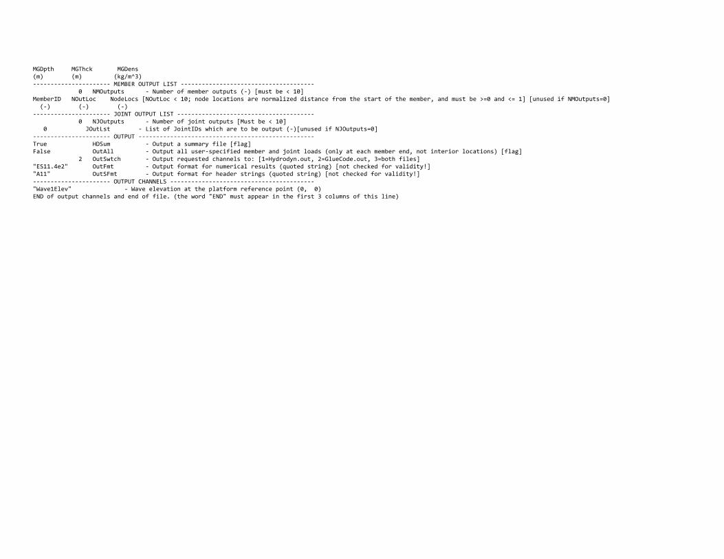
MGDpth MGThck MGDens (m) (m) (kg/m^3) ---------------------- MEMBER OUTPUT LIST -------------------------------------- 0 NMOutputs - Number of member outputs (-) [must be < 10] MemberID NOutLoc NodeLocs [NOutLoc < 10; node locations are normalized distance from the start of the member, and must be >=0 and <= 1] [unused if NMOutputs=0] (-) (-) (-) ---------------------- JOINT OUTPUT LIST --------------------------------------- 0 NJOutputs - Number of joint outputs [Must be < 10] 0 JOutLst - List of JointIDs which are to be output (-)[unused if NJOutputs=0] ---------------------- OUTPUT -------------------------------------------------- True HDSum - Output a summary file [flag] False OutAll - Output all user-specified member and joint loads (only at each member end, not interior locations) [flag] 2 OutSwtch - Output requested channels to: [1=Hydrodyn.out, 2=GlueCode.out, 3=both files] "ES11.4e2" OutFmt - Output format for numerical results (quoted string) [not checked for validity!] "A11" OutSFmt - Output format for header strings (quoted string) [not checked for validity!] ---------------------- OUTPUT CHANNELS ----------------------------------------- "Wave1Elev" - Wave elevation at the platform reference point (0, 0) END of output channels and end of file. (the word "END" must appear in the first 3 columns of this line)

Appendix B. OC4 Semi-submersible Driver File HydroDyn Driver file for OC4 Semi-submersible. Compatible with HydroDyn v2.01.* TRUE Echo - Echo the input file data (flag) ---------------------- ENVIRONMENTAL CONDITIONS ------------------------------- 9.80665 Gravity - Gravity (m/s^2) ---------------------- HYDRODYN ----------------------------------------------- "./OC4Semi.dat" HDInputFile - Primary HydroDyn input file name (quoted string) "./OC4Semi" OutRootName - The name which prefixes all HydroDyn generated files (quoted string) 1 NSteps - Number of time steps in the simulations (-) 0.025 TimeInterval - TimeInterval for the simulation (sec) ---------------------- WAMIT INPUTS ------------------------------------------- 1 WAMITInputsMod - Inputs model {0: all inputs are zero for every timestep, 1: steadystate inputs, 2: read inputs from a file (InputsFile)} (switch) "" WAMITInputsFile - Name of the inputs file if InputsMod = 2 (quoted string) ---------------------- WAMIT STEADY STATE INPUTS ----------------------------- 1.0 2.0 3.0 4.0 5.0 6.0 uWAMITInSteady - input displacements and rotations at the platform reference point (m, rads) 7.0 8.0 9.0 10.0 11.0 12.0 uDotWAMITInSteady - input translational and rotational velocities at the platform reference point (m/s, rads/s) 13.0 14.0 15.0 16.0 17.0 18.0 uDotDotWAMITInSteady - input translational and rotational acccelerations at the platform reference point (m/s^2, rads/s^2) ---------------------- MORISON INPUTS ----------------------------------------- 0 MorisonInputsMod - Inputs model {0: all inputs are zero for every timestep, 1: steadystate inputs, 2: read inputs from a file (InputsFile)} (switch) " " MorisonInputsFile - Name of the inputs file if InputsMod = 2 (quoted string) ---------------------- MORISON STEADY STATE INPUTS --------------------------- 1.0 2.0 3.0 4.0 5.0 6.0 uMorisonInSteady - input displacements and rotations for the morison elements (m, rads) 7.0 8.0 9.0 10.0 11.0 12.0 uDotMorisonInSteady - input translational and rotational velocities for the morison elements (m/s, rads/s) 13.0 14.0 15.0 16.0 17.0 18.0 uDotDotMorisonInSteady - input translational and rotational acccelerations for the morison elements (m/s^2, rads/s^2) ---------------------- Waves multipoint elevation output ------------------------------- TRUE WaveElevSeriesFlag - T/F flag to calculate the wave elevation field (for movies) 5.0 5.0 WaveElevDX WaveElevDY - WaveElevSeries spacing -- WaveElevDX WaveElevDY 3 3 WaveElevNX WaveElevNY - WaveElevSeries points -- WaveElevNX WaveElevNY END of driver input file

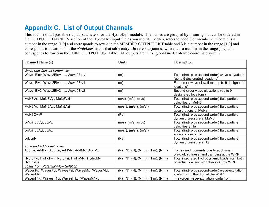
Appendix C. List of Output Channels This is a list of all possible output parameters for the HydroDyn module. The names are grouped by meaning, but can be ordered in the OUTPUT CHANNELS section of the HydroDyn input file as you see fit. MαNβ, refers to node β of member α, where α is a number in the range [1,9] and corresponds to row α in the MEMBER OUTPUT LIST table and β is a number in the range [1,9] and corresponds to location β in the NodeLocs list of that table entry. Jα refers to joint α, where α is a number in the range [1,9] and corresponds to row α in the JOINT OUTPUT LIST table. All outputs are in the global inertial-frame coordinate system.

Channel Name(s) Units Description

Wave and Current Kinematics Wave1Elev, Wave2Elev, …, Wave9Elev (m) Total (first- plus second-order) wave elevations

(up to 9 designated locations) Wave1Elv1, Wave2Elv1, …, Wave9Elv1 (m) First-order wave elevations (up to 9 designated

locations) Wave1Elv2, Wave2Elv2, …, Wave9Elv2 (m) Second-order wave elevations (up to 9

designated locations) MαNβVxi, MαNβVyi, MαNβVzi (m/s), (m/s), (m/s) Total (first- plus second-order) fluid particle

velocities at MαNβ MαNβAxi, MαNβAyi, MαNβAzi (m/s2), (m/s2), (m/s2) Total (first- plus second-order) fluid particle

accelerations at MαNβ MαNβDynP (Pa) Total (first- plus second-order) fluid particle

dynamic pressure at MαNβ JαVxi, JαVyi, JαVzi (m/s), (m/s), (m/s) Total (first- plus second-order) fluid particle

velocities at Jα JαAxi, JαAyi, JαAzi (m/s2), (m/s2), (m/s2) Total (first- plus second-order) fluid particle

accelerations at Jα JαDynP (Pa) Total (first- plus second-order) fluid particle

dynamic pressure at Jα Total and Additional Loads AddFxi, AddFyi, AddFzi, AddMxi, AddMyi, AddMzi (N), (N), (N), (N·m), (N·m), (N·m) Forces and moments due to additional

preload, stiffness, and damping at the WRP HydroFxi, HydroFyi, HydroFzi, HydroMxi, HydroMyi, HydroMzi

(N), (N), (N), (N·m), (N·m), (N·m) Total integrated hydrodynamic loads from both potential flow and strip theory at the WRP

Loads from Potential-Flow Solution WavesFxi, WavesFyi, WavesFzi, WavesMxi, WavesMyi, WavesMzi

(N), (N), (N), (N·m), (N·m), (N·m) Total (first- plus second-order) wave-excitation loads from diffraction at the WRP

WavesF1xi, WavesF1yi, WavesF1zi, WavesM1xi, (N), (N), (N), (N·m), (N·m), (N·m) First-order wave-excitation loads from

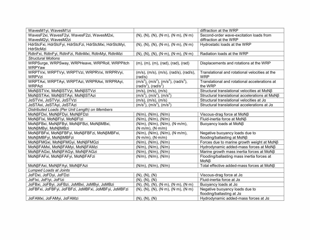
WavesM1yi, WavesM1zi diffraction at the WRP WavesF2xi, WavesF2yi, WavesF2zi, WavesM2xi, WavesM2yi, WavesM2zi

(N), (N), (N), (N·m), (N·m), (N·m) Second-order wave-excitation loads from diffraction at the WRP

HdrStcFxi, HdrStcFyi, HdrStcFzi, HdrStcMxi, HdrStcMyi, HdrStcMzi

(N), (N), (N), (N·m), (N·m), (N·m) Hydrostatic loads at the WRP

RdtnFxi, RdtnFyi, RdtnFzi, RdtnMxi, RdtnMyi, RdtnMzi (N), (N), (N), (N·m), (N·m), (N·m) Radiation loads at the WRP Structural Motions WRPSurge, WRPSway, WRPHeave, WRPRoll, WRPPitch WRPYaw

(m), (m), (m), (rad), (rad), (rad) Displacements and rotations at the WRP

WRPTVxi, WRPTVyi, WRPTVzi, WRPRVxi, WRPRVyi, WRPVzi

(m/s), (m/s), (m/s), (rad/s), (rad/s), (rad/s)

Translational and rotational velocities at the WRP

WRPTAxi, WRPTAyi, WRPTAzi, WRPRAxi, WRPRAyi, WRPAzi

(m/s2), (m/s2), (m/s2), (rad/s2), (rad/s2), (rad/s2)

Translational and rotational accelerations at the WRP

MαNβSTVxi, MαNβSTVyi, MαNβSTVzi (m/s), (m/s), (m/s) Structural translational velocities at MαNβ MαNβSTAxi, MαNβSTAyi, MαNβSTAzi (m/s2), (m/s2), (m/s2) Structural translational accelerations at MαNβ JαSTVxi, JαSTVyi, JαSTVzi (m/s), (m/s), (m/s) Structural translational velocities at Jα JαSTAxi, JαSTAyi, JαSTAzi (m/s2), (m/s2), (m/s2) Structural translational accelerations at Jα Distributed Loads (Per Unit Length) on Members MαNβFDxi, MαNβFDyi, MαNβFDzi (N/m), (N/m), (N/m) Viscous-drag force at MαNβ MαNβFIxi, MαNβFIyi, MαNβFIzi (N/m), (N/m), (N/m) Fluid-inertia force at MαNβ MαNβFBxi, MαNβFByi, MαNβFBzi, MαNβMBxi, MαNβMByi, MαNβMBzi

(N/m), (N/m), (N/m), (N·m/m), (N·m/m), (N·m/m)

Buoyancy loads at MαNβ

MαNβFBFxi, MαNβFBFyi, MαNβFBFzi, MαNβMBFxi, MαNβMBFyi, MαNβMBFzi

(N/m), (N/m), (N/m), (N·m/m), (N·m/m), (N·m/m)

Negative buoyancy loads due to flooding/ballasting at MαNβ

MαNβFMGxi, MαNβFMGyi, MαNβFMGzi (N/m), (N/m), (N/m) Forces due to marine growth weight at MαNβ MαNβFAMxi, MαNβFAMyi, MαNβFAMzi (N/m), (N/m), (N/m) Hydrodynamic added-mass forces at MαNβ MαNβFAGxi, MαNβFAGyi, MαNβFAGzi (N/m), (N/m), (N/m) Marine growth mass inertia forces at MαNβ MαNβFAFxi, MαNβFAFyi, MαNβFAFzi (N/m), (N/m), (N/m) Flooding/ballasting mass inertia forces at

MαNβ MαNβFAxi, MαNβFAyi, MαNβFAzi (N/m), (N/m), (N/m) Total effective added-mass forces at MαNβ Lumped Loads at Joints JαFDxi, JαFDyi, JαFDzi (N), (N), (N) Viscous-drag force at Jα JαFIxi, JαFIyi, JαFIzi (N), (N), (N) Fluid-inertia force at Jα JαFBxi, JαFByi, JαFBzi, JαMBxi, JαMByi, JαMBzi (N), (N), (N), (N·m), (N·m), (N·m) Buoyancy loads at Jα JαFBFxi, JαFBFyi, JαFBFzi, JαMBFxi, JαMBFyi, JαMBFzi (N), (N), (N), (N·m), (N·m), (N·m) Negative buoyancy loads due to

flooding/ballasting at Jα JαFAMxi, JαFAMyi, JαFAMzi (N), (N), (N) Hydrodynamic added-mass forces at Jα

Appendix D. Compiling Stand-alone HydroDyn See the FAST documentation for instructions on how to compile HydroDyn coupled to FAST.

Future versions of the manual will include compiling instructions for building the stand-along HydroDyn program.

Appendix E. Major Changes in HydroDyn HydroDyn when first released was included as an undocumented feature of FAST and packaged with the FAST archive. Since v2.00, the former software called “HydroDyn” has been separated into a distinct module packaged separately from FAST (but still coupled to FAST) and itself has been split into two pieces of software, each following the FAST modularization framework. This appendix outlines significant modifications to HydroDyn made with each public release, starting with v2.00.

V2.02 (September 2014) Version 2.02 integrates with the FAST v8 software v8.09.00a-bjj.

• Primary input file changes o 2ND-ORDER WAVES section

Removed WvMnDriftQTF option

Enabled WvDiffQTF and WvSumQTF options for calculating second-order wave kinematics for use in strip theory

o 2ND-ORDER FLOATING PLATFORM FORCES section

Enabled MnDrift, NewmanApp, DiffQTF, and SumQTF options for calculating second-order loads for use in potential-flow theory

• New or Modified Hydrodynamics o Added second-order wave kinematics for use in strip theory calculations

o Added second-order load calculations for use in potential-flow theory (second-order hydrodynamic coefficients must be supplied using WAMIT)

• Output file changes o Added output channels for first- and second-order wave elevation (Wave1Elv1,

Wave1Elv2, etc); changed the existing wave-elevation outputs (Wave1Elev, etc) to be the total wave elevation (i.e., the sum of the first- and second-order waves)

o Added output channels for first- and second-order wave loads from potential-flow calculations (WavesF1xi, WavesF2xi, etc); changed the existing wave load outputs (WavesFxi, etc) to be the total wave load (i.e., the sum of the first- and second-order wave loads)

• Significant bug Fixes o Fixed bug in the HydroDyn output file when coupled to FAST (multiple lines

were output)

o Fixed bug in output channel handling when compiled with gfortran

o Minor changes in Morison module to allow for compiling in double precision

o Fixed bug with multidirectional waves for single wave direction (WaveNDir = 1, or WaveDirSpread = 0)

v2.01 (June 2014) Version 2.01 integrates with the FAST v8 software v8.08.00c-bjj.

• Driver input file changes o Enabled MorisonInputsMod option for steady-state Morison inputs

o Added wave-elevation output section

• Primary input file changes o ENVIRONMENTAL CONDITIONS section

Enabled the MSL2SWL parameter

o WAVES section

Added parameters supporting multi-directional waves: WaveDirMod, WaveDirSpread, WaveNDir, WaveDirRange

o Added 2ND-ORDER WAVES section

o FLOATING PLATFORM section

Added support for RdtnDT to be set to “DEFAULT” to match driver code time step

o Added 2ND-ORDER FLOATING PLATFORM FORCES section

o HEAVE COEFFICIENTS section renamed AXIAL COEFFICIENTS

Renamed HvCoefID to AxCoefID

Renamed CdHv to AxCd

Renamed CaHv to AxCa

Added axial dynamic-pressure coefficient, AxCp

o SIMPLE HYDRODYNAMIC COEFFICIENTS section

Added dynamic-pressure coefficients: SimplCp, SimplCpMG

Added parameters for axial coefficients: SimplAxCa, SimplAxCaMG, SimplAxCp, SimplAxCpMG

o DEPTH-BASED HYDRODYNAMIC COEFFICIENTS section

Added dynamic-pressure coefficients: DpthCp, DpthCpMG

Added parameters for axial coefficients: DpthAxCa, DpthAxCaMG, DpthAxCp, DpthAxCpMG

o MEMBER-BASED HYDRODYNAMIC COEFFICIENTS section

Added dynamic-pressure coefficients: MemberCp1, MemberCp2, MemberCpMG1, MemberCpMG2,

Added parameters for axial coefficients: MemberAxCa1, MemberAxCa2, MemberAxCaMG1, MemberAxCaMG2,

MemberAxCp1, MemberAxCp2, MemberAxCpMG1, MemberAxCpMG2

o Consolidated the two sections for output channel labels into a single OUTPUT CHANNELS section.

Numerous changes and additions to the available channel labels, see Appendix C

• Output file changes o Modified file naming convention to match FAST convention

o Summary file saw several changes

Now includes WAMIT-body volume and buoyancy table

Existing volume, buoyancy, and weight tables were moved to the start of the file

The radiation kernel and wave kinematics tables were moved to the end of the file

The node and element tables were altered

New wave-elevation outputs file available when using stand-alone HydroDyn

All units are now SI (m, N, s)

o Results file

All units are now SI (m, N, s)

• New or Modified Hydrodynamics o Added multi-directional waves

o Combined Froude-Kriloff (dynamic-pressure) loads into the inertial loads

o Added option whereby if simulation time is greater than WaveTMax, waves repeat

o Added lumped inertial loads

o Altered lumped added-mass equation

o Altered distributed inertial-load equation

o Altered fluid-domain checks for when to compute hydrodynamic loads

o Included the platform added-mass loads in the radiation load outputs (RdtnFxi, RdtnFyi, etc.)

• Miscellaneous o Restructured the calculation of loads due to additional stiffness, damping so they

work when HasWAMIT = FALSE

o Wave elevations can now be output when HasWAMIT = FALSE

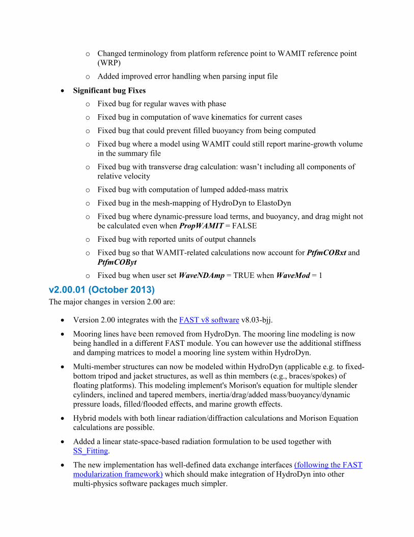
o Changed terminology from platform reference point to WAMIT reference point (WRP)

o Added improved error handling when parsing input file

• Significant bug Fixes o Fixed bug for regular waves with phase

o Fixed bug in computation of wave kinematics for current cases

o Fixed bug that could prevent filled buoyancy from being computed

o Fixed bug where a model using WAMIT could still report marine-growth volume in the summary file

o Fixed bug with transverse drag calculation: wasn’t including all components of relative velocity

o Fixed bug with computation of lumped added-mass matrix

o Fixed bug in the mesh-mapping of HydroDyn to ElastoDyn

o Fixed bug where dynamic-pressure load terms, and buoyancy, and drag might not be calculated even when PropWAMIT = FALSE

o Fixed bug with reported units of output channels

o Fixed bug so that WAMIT-related calculations now account for PtfmCOBxt and PtfmCOByt

o Fixed bug when user set WaveNDAmp = TRUE when WaveMod = 1

v2.00.01 (October 2013) The major changes in version 2.00 are:

• Version 2.00 integrates with the FAST v8 software v8.03-bjj.

• Mooring lines have been removed from HydroDyn. The mooring line modeling is now being handled in a different FAST module. You can however use the additional stiffness and damping matrices to model a mooring line system within HydroDyn.

• Multi-member structures can now be modeled within HydroDyn (applicable e.g. to fixed-bottom tripod and jacket structures, as well as thin members (e.g., braces/spokes) of floating platforms). This modeling implement's Morison's equation for multiple slender cylinders, inclined and tapered members, inertia/drag/added mass/buoyancy/dynamic pressure loads, filled/flooded effects, and marine growth effects.

• Hybrid models with both linear radiation/diffraction calculations and Morison Equation calculations are possible.

• Added a linear state-space-based radiation formulation to be used together with SS_Fitting.

• The new implementation has well-defined data exchange interfaces (following the FAST modularization framework) which should make integration of HydroDyn into other multi-physics software packages much simpler.