SANDIA REPORTSAND2021-5812Printed May 2021

Prepared bySandia National LaboratoriesAlbuquerque, New Mexico 87185Livermore, California 94550

Hydrogen Risk Assessment Models(HyRAM) Version 3.1 Technical ReferenceManualBrian D. Ehrhart, Ethan S. Hecht

Issued by Sandia National Laboratories, operated for the United States Department of Energy by NationalTechnology & Engineering Solutions of Sandia, LLC.

NOTICE: This report was prepared as an account of work sponsored by an agency of the United States Government.Neither the United States Government, nor any agency thereof, nor any of their employees, nor any of theircontractors, subcontractors, or their employees, make any warranty, express or implied, or assume any legal liabilityor responsibility for the accuracy, completeness, or usefulness of any information, apparatus, product, or processdisclosed, or represent that its use would not infringe privately owned rights. Reference herein to any specificcommercial product, process, or service by trade name, trademark, manufacturer, or otherwise, does not necessarilyconstitute or imply its endorsement, recommendation, or favoring by the United States Government, any agencythereof, or any of their contractors or subcontractors. The views and opinions expressed herein do not necessarilystate or reflect those of the United States Government, any agency thereof, or any of their contractors.

Printed in the United States of America. This report has been reproduced directly from the best available copy.

Available to DOE and DOE contractors from

U.S. Department of EnergyOffice of Scientific and Technical InformationP.O. Box 62Oak Ridge, TN 37831

Telephone: (865) 576-8401Facsimile: (865) 576-5728E-Mail: reports@osti.govOnline ordering: http://www.osti.gov/scitech

Available to the public from

U.S. Department of CommerceNational Technical Information Service5301 Shawnee RoadAlexandria, VA 22312

Telephone: (800) 553-6847Facsimile: (703) 605-6900E-Mail: orders@ntis.govOnline order: https://classic.ntis.gov/help/order-methods

DE

PA

RT

MENT OF EN

ER

GY

• • UN

IT

ED

STATES OFA

M

ER

IC

A

2

ABSTRACT

The HyRAM software toolkit provides a basis for conducting quantitative risk assessment andconsequence modeling for hydrogen infrastructure and transportation systems. HyRAM isdesigned to facilitate the use of state-of-the-art science and engineering models to conduct robust,repeatable assessments of hydrogen safety, hazards, and risk. HyRAM includes genericprobabilities for hydrogen equipment failures, probabilistic models for the impact of heat flux onhumans and structures, and experimentally validated first-order models of hydrogen release andflame physics. HyRAM integrates deterministic and probabilistic models for quantifying accidentscenarios, predicting physical effects, and characterizing hydrogen hazards (thermal effects fromjet fires, overpressure effects from deflagrations), and assessing impact on people and structures.HyRAM is developed at Sandia National Laboratories for the U.S. Department of Energy toincrease access to technical data about hydrogen safety and to enable the use of that data tosupport development and revision of national and international codes and standards. HyRAM is aresearch software in active development and thus the models and data may change. This reportwill be updated at appropriate developmental intervals.

This document provides a description of the methodology and models contained in HyRAMversion 3.1. There have been several impactful updates since version 3.0. HyRAM 3.1 contains acorrection to use the volume fraction for two-phase speed of sound calculations; this only affectscryogenic releases in which two-phase flow (vapor and liquid) is predicted in the orifice. Otherchanges include clarifications that inputs for tank pressure should be given in absolute pressure,not gauge pressure. Additionally, the interface now rejects invalid inputs to probabilitydistributions, and the less accurate single-point radiative source model selection was removedfrom the interface.

3

ACKNOWLEDGMENT

This report describes a revised version of the HyRAM code, which itself was built upon theprevious work of many others. The authors therefore especially wish to thank Katrina Groth (nowat the University of Maryland) for her leadership and contributions to the HyRAM code andproject, as well as John Reynolds, Myra Blaylock, and Erin Carrier for their contributions. Theauthors wish to thank Cianan Sims of Sims Industries for his contributions to the HyRAM code.This work was supported by the U.S. Department of Energy (DOE) Office of Energy Efficiency(EERE) Hydrogen and Fuel Cell Technologies Office (HFTO). The authors gratefullyacknowledge Chris LaFleur, Dusty Brooks, and Alice Muna at Sandia for helpful discussions anduseful insights. The authors also wish to specifically thank the members of NFPA 2, the HydrogenSafety Panel, and HySafe for engaging technical discussions and thoughtful feedback. Finally, theauthors gratefully acknowledge the many productive discussions with users, other researchers,and the various stakeholders who have provided insight and feedback for this work.

4

CONTENTS

1. Introduction . . . . . . . . . . . . . . . . . . . . . . . . . . . . . . . . . . . . . . . . . . . . . . . . . . . . . . . . . . . . . . . . . 91.1. About HyRAM and This Report . . . . . . . . . . . . . . . . . . . . . . . . . . . . . . . . . . . . . . . . . . . 91.2. Background and Motivation . . . . . . . . . . . . . . . . . . . . . . . . . . . . . . . . . . . . . . . . . . . . . . . 91.3. Design Goals and Limitations . . . . . . . . . . . . . . . . . . . . . . . . . . . . . . . . . . . . . . . . . . . . . 101.4. Summary of HyRAM Outputs . . . . . . . . . . . . . . . . . . . . . . . . . . . . . . . . . . . . . . . . . . . . . 101.5. Summary of Changes Made . . . . . . . . . . . . . . . . . . . . . . . . . . . . . . . . . . . . . . . . . . . . . . . 11

2. Quantitative Risk Assessment Methodology . . . . . . . . . . . . . . . . . . . . . . . . . . . . . . . . . . . . . . 132.1. Quantitative Risk Assessment Methodology Overview . . . . . . . . . . . . . . . . . . . . . . . . 132.2. Risk Metrics Calculations . . . . . . . . . . . . . . . . . . . . . . . . . . . . . . . . . . . . . . . . . . . . . . . . 142.3. Scenario Models . . . . . . . . . . . . . . . . . . . . . . . . . . . . . . . . . . . . . . . . . . . . . . . . . . . . . . . . 15

2.3.1. Default Detection and Isolation Probability . . . . . . . . . . . . . . . . . . . . . . . . . . . 162.3.2. Default Ignition Probabilities . . . . . . . . . . . . . . . . . . . . . . . . . . . . . . . . . . . . . . . 17

2.4. Frequency of a Hydrogen Release . . . . . . . . . . . . . . . . . . . . . . . . . . . . . . . . . . . . . . . . . . 172.4.1. Frequency of Random Leaks . . . . . . . . . . . . . . . . . . . . . . . . . . . . . . . . . . . . . . . 182.4.2. Default Component Leak Frequencies . . . . . . . . . . . . . . . . . . . . . . . . . . . . . . . 182.4.3. Frequency of Dispenser Releases . . . . . . . . . . . . . . . . . . . . . . . . . . . . . . . . . . . . 212.4.4. Default Dispenser Failure Probabilities . . . . . . . . . . . . . . . . . . . . . . . . . . . . . . . 24

2.5. Consequence Models . . . . . . . . . . . . . . . . . . . . . . . . . . . . . . . . . . . . . . . . . . . . . . . . . . . . 252.5.1. Facility Occupants . . . . . . . . . . . . . . . . . . . . . . . . . . . . . . . . . . . . . . . . . . . . . . . . 252.5.2. Jet Fire . . . . . . . . . . . . . . . . . . . . . . . . . . . . . . . . . . . . . . . . . . . . . . . . . . . . . . . . . 262.5.3. Explosion (Deflagration or Detonation) Overpressure . . . . . . . . . . . . . . . . . . . 262.5.4. Default Overpressure and Impulse Values . . . . . . . . . . . . . . . . . . . . . . . . . . . . 26

2.6. Harm and Loss Models . . . . . . . . . . . . . . . . . . . . . . . . . . . . . . . . . . . . . . . . . . . . . . . . . . . 272.6.1. Thermal Harm . . . . . . . . . . . . . . . . . . . . . . . . . . . . . . . . . . . . . . . . . . . . . . . . . . . 272.6.2. Overpressure Harm . . . . . . . . . . . . . . . . . . . . . . . . . . . . . . . . . . . . . . . . . . . . . . . 28

3. Physics Models . . . . . . . . . . . . . . . . . . . . . . . . . . . . . . . . . . . . . . . . . . . . . . . . . . . . . . . . . . . . . . 293.1. Properties of Hydrogen . . . . . . . . . . . . . . . . . . . . . . . . . . . . . . . . . . . . . . . . . . . . . . . . . . . 29

3.1.1. Equation of State . . . . . . . . . . . . . . . . . . . . . . . . . . . . . . . . . . . . . . . . . . . . . . . . . 293.1.2. Combustion . . . . . . . . . . . . . . . . . . . . . . . . . . . . . . . . . . . . . . . . . . . . . . . . . . . . . 30

3.2. Developing Flow . . . . . . . . . . . . . . . . . . . . . . . . . . . . . . . . . . . . . . . . . . . . . . . . . . . . . . . . 323.2.1. Orifice Flow . . . . . . . . . . . . . . . . . . . . . . . . . . . . . . . . . . . . . . . . . . . . . . . . . . . . . 323.2.2. Notional Nozzles . . . . . . . . . . . . . . . . . . . . . . . . . . . . . . . . . . . . . . . . . . . . . . . . . 343.2.3. Initial Entrainment and Heating . . . . . . . . . . . . . . . . . . . . . . . . . . . . . . . . . . . . . 363.2.4. Establishment of a Gaussian Profile . . . . . . . . . . . . . . . . . . . . . . . . . . . . . . . . . 37

3.3. Unignited Releases . . . . . . . . . . . . . . . . . . . . . . . . . . . . . . . . . . . . . . . . . . . . . . . . . . . . . . 383.3.1. Gas Jet/Plume . . . . . . . . . . . . . . . . . . . . . . . . . . . . . . . . . . . . . . . . . . . . . . . . . . . 383.3.2. Tank Emptying . . . . . . . . . . . . . . . . . . . . . . . . . . . . . . . . . . . . . . . . . . . . . . . . . . . 413.3.3. Accumulation in Confined Areas/Enclosures . . . . . . . . . . . . . . . . . . . . . . . . . . 42

3.4. Ignited Releases . . . . . . . . . . . . . . . . . . . . . . . . . . . . . . . . . . . . . . . . . . . . . . . . . . . . . . . . . 433.4.1. Flame Correlations . . . . . . . . . . . . . . . . . . . . . . . . . . . . . . . . . . . . . . . . . . . . . . . 433.4.2. Radiation From a Straight Flame . . . . . . . . . . . . . . . . . . . . . . . . . . . . . . . . . . . . 45

5

3.4.3. Jet Flame with Buoyancy Correction . . . . . . . . . . . . . . . . . . . . . . . . . . . . . . . . . 463.4.4. Radiation From a Curved Flame . . . . . . . . . . . . . . . . . . . . . . . . . . . . . . . . . . . . 473.4.5. Overpressure in Enclosures . . . . . . . . . . . . . . . . . . . . . . . . . . . . . . . . . . . . . . . . 48

4. Summary of Numerical Methods . . . . . . . . . . . . . . . . . . . . . . . . . . . . . . . . . . . . . . . . . . . . . . . 494.1. Python Calculation Methods . . . . . . . . . . . . . . . . . . . . . . . . . . . . . . . . . . . . . . . . . . . . . . 494.2. Leak Frequency Computations . . . . . . . . . . . . . . . . . . . . . . . . . . . . . . . . . . . . . . . . . . . . 494.3. Unit Conversion . . . . . . . . . . . . . . . . . . . . . . . . . . . . . . . . . . . . . . . . . . . . . . . . . . . . . . . . . 49

5. Engineering Toolkit . . . . . . . . . . . . . . . . . . . . . . . . . . . . . . . . . . . . . . . . . . . . . . . . . . . . . . . . . . 515.1. Temperature, Pressure, and Density . . . . . . . . . . . . . . . . . . . . . . . . . . . . . . . . . . . . . . . . 515.2. Tank Mass . . . . . . . . . . . . . . . . . . . . . . . . . . . . . . . . . . . . . . . . . . . . . . . . . . . . . . . . . . . . . 515.3. Mass Flow Rate . . . . . . . . . . . . . . . . . . . . . . . . . . . . . . . . . . . . . . . . . . . . . . . . . . . . . . . . . 515.4. TNT Mass Equivalence . . . . . . . . . . . . . . . . . . . . . . . . . . . . . . . . . . . . . . . . . . . . . . . . . . 52

References . . . . . . . . . . . . . . . . . . . . . . . . . . . . . . . . . . . . . . . . . . . . . . . . . . . . . . . . . . . . . . . . . . . . . 53

LIST OF FIGURES

Figure 2-1. Summary of QRA methodology implemented in HyRAM toolkit . . . . . . . . . . . . 14Figure 2-2. Event sequence diagram used by HyRAM for H2 releases . . . . . . . . . . . . . . . . . . . 16Figure 2-3. Fault tree for random leaks of size 0.01% from H2 components . . . . . . . . . . . . . . . 18Figure 2-4. Fault Tree for Other Releases from a Dispenser . . . . . . . . . . . . . . . . . . . . . . . . . . . . 22Figure 3-1. Graphical representations of state points, calculated using CoolProp [1] which

is referencing the Leachman et al. [2] equation of state for hydrogen. Top plotsshow shading and iso-contours of density as a funciton of temperature and pres-sure. Bottom plot shows shading of density, with iso-contours of pressure andenthalpy. . . . . . . . . . . . . . . . . . . . . . . . . . . . . . . . . . . . . . . . . . . . . . . . . . . . . . . . . . . . . 30

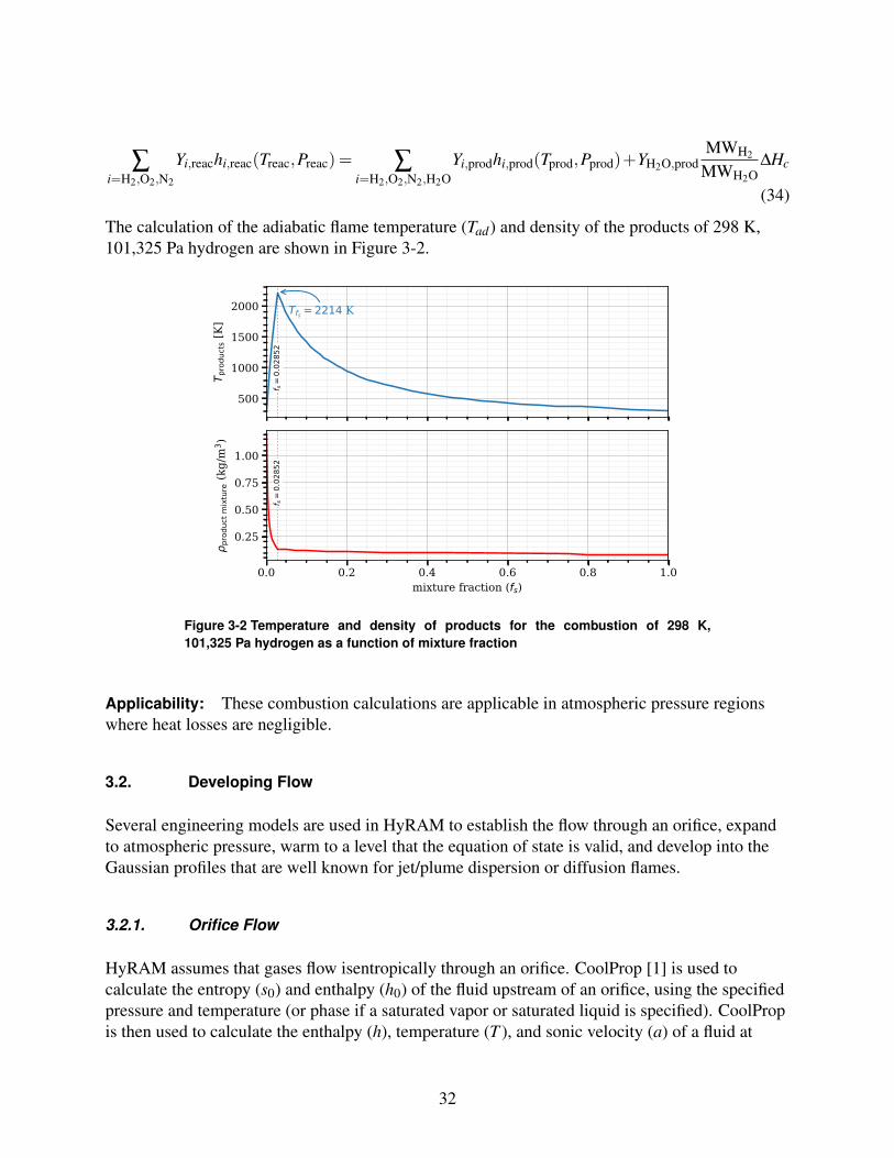
Figure 3-2. Temperature and density of products for the combustion of 298 K, 101,325 Pahydrogen as a function of mixture fraction . . . . . . . . . . . . . . . . . . . . . . . . . . . . . . . . 32

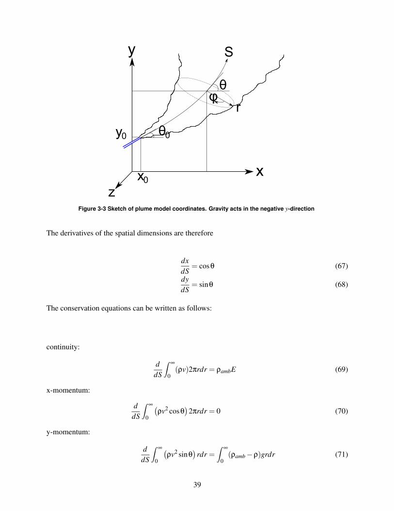
Figure 3-3. Sketch of plume model coordinates. Gravity acts in the negative y-direction . . . . 39

LIST OF TABLES

Table 2-1. Ignition Probabilities . . . . . . . . . . . . . . . . . . . . . . . . . . . . . . . . . . . . . . . . . . . . . . . . . . . 17Table 2-2. Parameters for frequency of random leaks for individual components . . . . . . . . . . . 20Table 2-3. Default Probability Distributions for Component Failure . . . . . . . . . . . . . . . . . . . . . 25Table 2-4. Default Probability Distributions for Accident Occurrence . . . . . . . . . . . . . . . . . . . . 25Table 2-5. Peak Overpressure and Impulse Values . . . . . . . . . . . . . . . . . . . . . . . . . . . . . . . . . . . . 26Table 2-6. Probit models used to calculate fatality probability as a function of thermal dose

(V ) . . . . . . . . . . . . . . . . . . . . . . . . . . . . . . . . . . . . . . . . . . . . . . . . . . . . . . . . . . . . . . . . . . 27Table 2-7. Probit models to calculate fatality probability from exposure to overpressures,

where Ps is peak overpressure (Pa) and i is the impulse of the shock wave (Pa·s) . 28

6

Table 4-1. HyRAM Convertible Units . . . . . . . . . . . . . . . . . . . . . . . . . . . . . . . . . . . . . . . . . . . . . . 49

7

ACRONYMS AND DEFINITIONS

AIR average individual risk

C&S codes and standards

CFD computational fluid dynamics

DOE U.S. Department of Energy

EERE Office of Energy Efficiency and Renewable Energy

ESD event sequence diagram

FAR fatal accident rate

H2 hydrogen

HFTO Hydrogen and Fuel Cell Technologies Office

HSE U.K. Health and Safety Executive

HyRAM Hydrogen Risk Assessment Models

ISO International Organization for Standardization

MW molecular weight

NFPA National Fire Protection Association

PLL potential loss of life

QRA quantitative risk assessment

SI International System of Units

TNO Netherlands Organisation for Applied Scientific Research

TNT trinitrotoluene

8

1. INTRODUCTION

1.1. About HyRAM and This Report

HyRAM (Hydrogen Risk Assessment Models) is a software toolkit that integrates data andmethods relevant to assessing the safety of hydrogen use, delivery, and storage infrastructure.HyRAM provides a platform which integrates state-of-the-art, validated science and engineeringmodels and data relevant to hydrogen safety into a comprehensive, industry-focused platform.The HyRAM risk assessment calculation incorporates generic probabilities for equipment failuresfor nine types of components, and probabilistic models for the effect of heat flux and overpressureon humans and structures. HyRAM also incorporates experimentally validated models of variousaspects of hydrogen release and flame physics. The HyRAM toolkit can be used to supportmultiple types of analysis, including code and standards development, safety basis development,and facility safety planning. HyRAM was developed by Sandia National Laboratories for the U.S.Department of Energy (DOE) Office of Energy Efficiency and Renewable Energy (EERE)Hydrogen and Fuel Cell Technologies Office (HFTO).

This report provides technical documentation of the algorithms, models, and data incorporated inHyRAM verion 3.1. HyRAM is free and open source software: you can redistribute it and/ormodify it under the terms of the GNU General Public License version 3, as published by the FreeSoftware Foundation. This program is distributed in the hope that it will be useful, butWITHOUT ANY WARRANTY; without even the implied warranty of MERCHANTABILITY orFITNESS FOR A PARTICULAR PURPOSE. See the GNU General Public License for moredetails (https://www.gnu.org/licenses/gpl-3.0.html).

1.2. Background and Motivation

Hydrogen has a variety of uses in the industrial, chemical, transportation, and electric powersectors. As with all fuels, regulations, codes, and standards are a necessary component of the safedeployment of hydrogen technologies. There has been a focused effort in both the U.S. andinternational hydrogen communities to develop codes and standards based on strong scientificprinciples to accommodate the relatively rapid deployment of hydrogen-energy systems.

Both quantitative risk assessment (QRA) and deterministic hydrogen behavior modeling havebecome valuable tools for the development and revision of hydrogen codes and standards such asNFPA 2, NFPA 55, and ISO TR-19880 [3–9]. However, the use of QRA in hydrogen applicationscurrently suffers from limitations and inefficiency due to a range of factors, including widevariation in QRA and consequence modeling approaches, the use of unvalidated physics models,lack of data, and more [10–15].

The development of HyRAM is meant to enable code development committees and other users toconduct QRA, hazard, and consequence analyses using a fast-running, comprehensivemethodology based in science and engineering models from the hydrogen safety researchcommunity [10, 16]. The HyRAM software toolkit provides a common methodology forconducting QRA with integrated reduced-order (simplified) physical models. A consistent,

9

documented methodology and corresponding software toolkit facilitates comparison of resultsbetween different stakeholders.

1.3. Design Goals and Limitations

HyRAM is designed to calculate multiple risk and harm/damage metrics from user-definedsystem configurations to provide insights for decision makers in the safety, codes, and standardscommunity. HyRAM contains generic industry-wide default inputs and fast-running,reduced-order models designed to facilitate comparison of different system designs andrequirements. Reduced-order models use simplyfing assumptions to approximate behavior muchmore quickly than more complex high-fidelity models. As such, the focus of HyRAM is onenabling systematic, defensible risk and consequence assessments for use in risk comparisons andsensitivity analyses, rather than on establishing the "true" frequency or risk of a hypotheticalaccident. HyRAM is designed to produce realistic best estimates for use in decision-making.

Note: Risk and safety assessment results should be used as part of a decision process, not as thesole basis for a decision. Safety and design decisions involve consideration of many factors andjudgments; these factors include the safety assessments, the assumptions and limitations of safetyassessments, the benefits of a technology, and public preferences. As such, HyRAM does notallow the user to specify an acceptability or tolerability criteria for risk or harm. Further guidanceon QRA and tolerability criteria can be found in the references [17–24].

HyRAM is designed to enable defensible, repeatable calculations using consistent, documentedalgorithms. The algorithms, models, and data in HyRAM have been assembled from published,publicly available sources. The physics models contained in HyRAM have been validated againstavailable experimental data [25]. Where model validation is not possible (e.g., for harm models),HyRAM is designed to allow users to choose among different models. HyRAM includes genericdata for hydrogen component leak frequencies and documented, expert-assigned probabilities forignition. HyRAM is designed to allow users to replace the default data and assumptions withsystem-specific information when such information is available to the user.

1.4. Summary of HyRAM Outputs

The QRA mode in HyRAM can be used to calculate three well-known risk metrics which arecommonly used to evaluate fatality risk in multiple industries, as well as other risk-relatedmetrics:

• FAR (Fatal Accident Rate) – the expected number of fatalities in 100 million exposed hours;• AIR (Average Individual Risk) – the expected number of fatalities per exposed individual;• PLL (Potential Loss of Life) – the expected number of fatalities per system-year;• Expected number of hydrogen releases per system-year (unignited and ignited cases);• Expected number of jet fires per system-year (immediate ignition cases);• Expected number of deflagrations/explosions per system-year (delayed ignition cases).

10

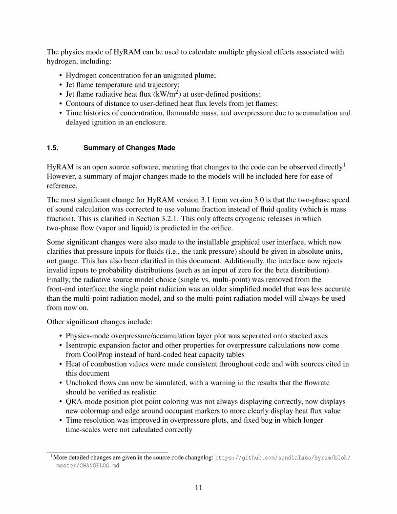
The physics mode of HyRAM can be used to calculate multiple physical effects associated withhydrogen, including:

• Hydrogen concentration for an unignited plume;• Jet flame temperature and trajectory;• Jet flame radiative heat flux (kW/m2) at user-defined positions;• Contours of distance to user-defined heat flux levels from jet flames;• Time histories of concentration, flammable mass, and overpressure due to accumulation and

delayed ignition in an enclosure.

1.5. Summary of Changes Made

HyRAM is an open source software, meaning that changes to the code can be observed directly1.However, a summary of major changes made to the models will be included here for ease ofreference.

The most significant change for HyRAM version 3.1 from version 3.0 is that the two-phase speedof sound calculation was corrected to use volume fraction instead of fluid quality (which is massfraction). This is clarified in Section 3.2.1. This only affects cryogenic releases in whichtwo-phase flow (vapor and liquid) is predicted in the orifice.

Some significant changes were also made to the installable graphical user interface, which nowclarifies that pressure inputs for fluids (i.e., the tank pressure) should be given in absolute units,not gauge. This has also been clarified in this document. Additionally, the interface now rejectsinvalid inputs to probability distributions (such as an input of zero for the beta distribution).Finally, the radiative source model choice (single vs. multi-point) was removed from thefront-end interface; the single point radiation was an older simplified model that was less accuratethan the multi-point radiation model, and so the multi-point radiation model will always be usedfrom now on.

Other significant changes include:

• Physics-mode overpressure/accumulation layer plot was seperated onto stacked axes• Isentropic expansion factor and other properties for overpressure calculations now come

from CoolProp instead of hard-coded heat capacity tables• Heat of combustion values were made consistent throughout code and with sources cited in

this document• Unchoked flows can now be simulated, with a warning in the results that the flowrate

should be verified as realistic• QRA-mode position plot point coloring was not always displaying correctly, now displays

new colormap and edge around occupant markers to more clearly display heat flux value• Time resolution was improved in overpressure plots, and fixed bug in which longer

time-scales were not calculated correctly

1More detailed changes are given in the source code changelog: https://github.com/sandialabs/hyram/blob/master/CHANGELOG.md

11

• Distributed version of Python is now 3.9 and installer now uses the WiX toolset (whichshould make future updates less time consuming)

12

2. QUANTITATIVE RISK ASSESSMENT METHODOLOGY

HyRAM includes a QRA mode, which provides calculations and models relevant to estimatingthe risk of hydrogen releases. The consequences and fatality risk of jet flames and overpressuresare estimated for different release sizes, each of which can be calculated to occur with differentfrequencies. These calculations use a subset of the models used in the physics mode to estimatethe release behavior (see Section 3).

2.1. Quantitative Risk Assessment Methodology Overview

In a QRA, multiple integrated models are used to provide a framework for reasoning aboutdecision options, based on the background information encoded in those models.

Risk is characterized by a set of hazard exposure scenarios (i), the consequences (ci) associatedwith each scenario, and the probability of occurrence (pi) of these consequences. One commonlyused expression for calculating risk is:

Risk = ∑i(pi× ci) (1)

In a QRA, the consequences are expressed in terms of an observable quantity, such as number offatalities or repair cost in a specific period of time. In HyRAM, the number of fatalties is used asthe safety metric of interest. The probability term (pi) expresses the analyst’s uncertainty aboutpredicted consequences (which encompasses the frequency of different scenarios and the range ofpossible consequences for each scenario).

The major elements of the QRA methodology in HyRAM are shown in Figure 2-1.

13

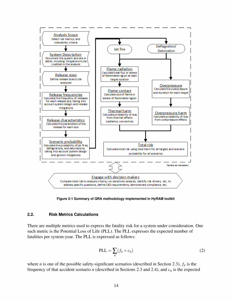
Figure 2-1 Summary of QRA methodology implemented in HyRAM toolkit

2.2. Risk Metrics Calculations

There are multiple metrics used to express the fatality risk for a system under consideration. Onesuch metric is the Potential Loss of Life (PLL). The PLL expresses the expected number offatalities per system-year. The PLL is expressed as follows:

PLL = ∑n( fn× cn) (2)

where n is one of the possible safety-significant scenarios (described in Section 2.3), fn is thefrequency of that accident scenario n (described in Sections 2.3 and 2.4), and cn is the expected

14

number of fatalities for accident scenario n (described in Section 2.6).

Another metric related to the PLL is the Fatal Accident Rate (FAR). The FAR is the expectednumber of fatalities in a group, per 100 million exposed hours. The FAR for a particular facilitycan be calculated using the PLL, as well as the population of the facility. The FAR is calculatedusing Equation 3.

FAR =PLL×108

Exposed hours=

PLL×108

Npop×8760(3)

where Npop is the average number of personnel in the facility, and dividing by 8760 converts fromyears to hours (24 hours per day and 365 days per year).

The third metric used in HyRAM is the Average Individual Risk (AIR). The AIR expresses theaverage number of fatalities per exposed individual. It is based on the number of hours theaverage occupant spends at the facility.

AIR = H×FAR×10−8 (4)

where H is the annual number of hours the individual spends in the facility (e.g., 2000 hours forfull-time worker).

2.3. Scenario Models

A release of hydrogen could lead to several different physical consequences and associatedhazards. For continuous releases of hydrogen, the physical consequences are unignited releases,jet fires (thermal effects), flash fires (deflagration of accumulated gas, dominated by thermaleffects), and explosions (deflagration or detonation of accumulated gas dominated byoverpressure effects). Currently, HyRAM calculates harm from thermal effects of jet fires (forimmediate ignition) and overpressure (for delayed ignition)2. A release of liquid hydrogen mayalso form a pool on the ground, but this is currently not considered in HyRAM. These scenariosare modeled in the event sequence diagram (ESD) for release of hydrogen (see Figure 2-2).

2Future versions of HyRAM may take account for the differences between thermal effects and overpressure effectsfor delayed ignition, but this is not currently included

15

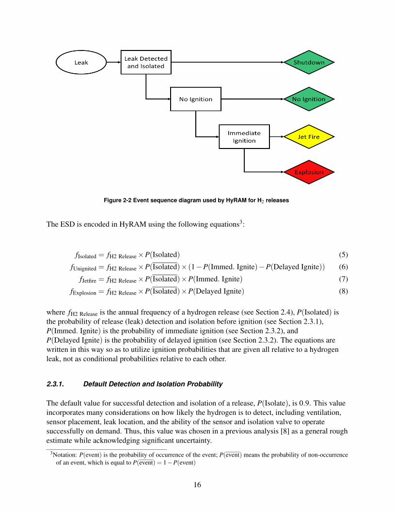
Figure 2-2 Event sequence diagram used by HyRAM for H2 releases

The ESD is encoded in HyRAM using the following equations3:

fIsolated = fH2 Release×P(Isolated) (5)

fUnignited = fH2 Release×P(Isolated)× (1−P(Immed. Ignite)−P(Delayed Ignite)) (6)

fJetfire = fH2 Release×P(Isolated)×P(Immed. Ignite) (7)

fExplosion = fH2 Release×P(Isolated)×P(Delayed Ignite) (8)

where fH2 Release is the annual frequency of a hydrogen release (see Section 2.4), P(Isolated) isthe probability of release (leak) detection and isolation before ignition (see Section 2.3.1),P(Immed. Ignite) is the probability of immediate ignition (see Section 2.3.2), andP(Delayed Ignite) is the probability of delayed ignition (see Section 2.3.2). The equations arewritten in this way so as to utilize ignition probabilities that are given all relative to a hydrogenleak, not as conditional probabilities relative to each other.

2.3.1. Default Detection and Isolation Probability

The default value for successful detection and isolation of a release, P(Isolate), is 0.9. This valueincorporates many considerations on how likely the hydrogen is to detect, including ventilation,sensor placement, leak location, and the ability of the sensor and isolation valve to operatesuccessfully on demand. Thus, this value was chosen in a previous analysis [8] as a general roughestimate while acknowledging significant uncertainty.

3Notation: P(event) is the probability of occurrence of the event; P(event) means the probability of non-occurrenceof an event, which is equal to P(event) = 1−P(event)

16

Note: This value can vary significantly based on a particular system setup, and so theuser/analyst needs to carefuly consider the particulars of the system being assessed and decide ifthis default value is appropriate.

2.3.2. Default Ignition Probabilities

The default hydrogen ignition probabilities are a function of hydrogen release rate and are givenin Table 2-1; these values are taken directly from [15]. It should be noted that both the immediateand dealyed ignition probabilities are independant and both relative to a hydrogen release; thedelayed ignition probability is not conditional upon the immediate ignition having not occured.The total probability of ignition of hydrogen is the immediate and delayed ignition probabilitiesadded together.

Table 2-1 Ignition ProbabilitiesH2 Release Rate (kg/s) P(Immediate Ignition) P(Delayed Ignition)

<0.125 0.008 0.0040.125 - 6.25 0.053 0.027

>6.25 0.230 0.120

2.4. Frequency of a Hydrogen Release

HyRAM calculates the annual frequency of a hydrogen release for release sizes of 0.01%, 0.1%,1%, 10%, or 100%. These release sizes are relative to the pipe flow area (A) as shown inEquation 9, where d is the inner diameter of the pipe4.

A =π

4d2 (9)

The annual frequency of a hydrogen release for each of the four smallest releases sizes (k =0.01%, 0.1%, 1%, and 10%) is given by:

fH2 Release,k = fRandom Releases,k (10)

The annual frequency of the largest release size (100%) is given by:

fH2 Release, k=100% = fRandom Releases,k=100% + fOther Releases (11)

4The discharge coefficient used in QRA mode is 1.0 and cannot currently be changed

17

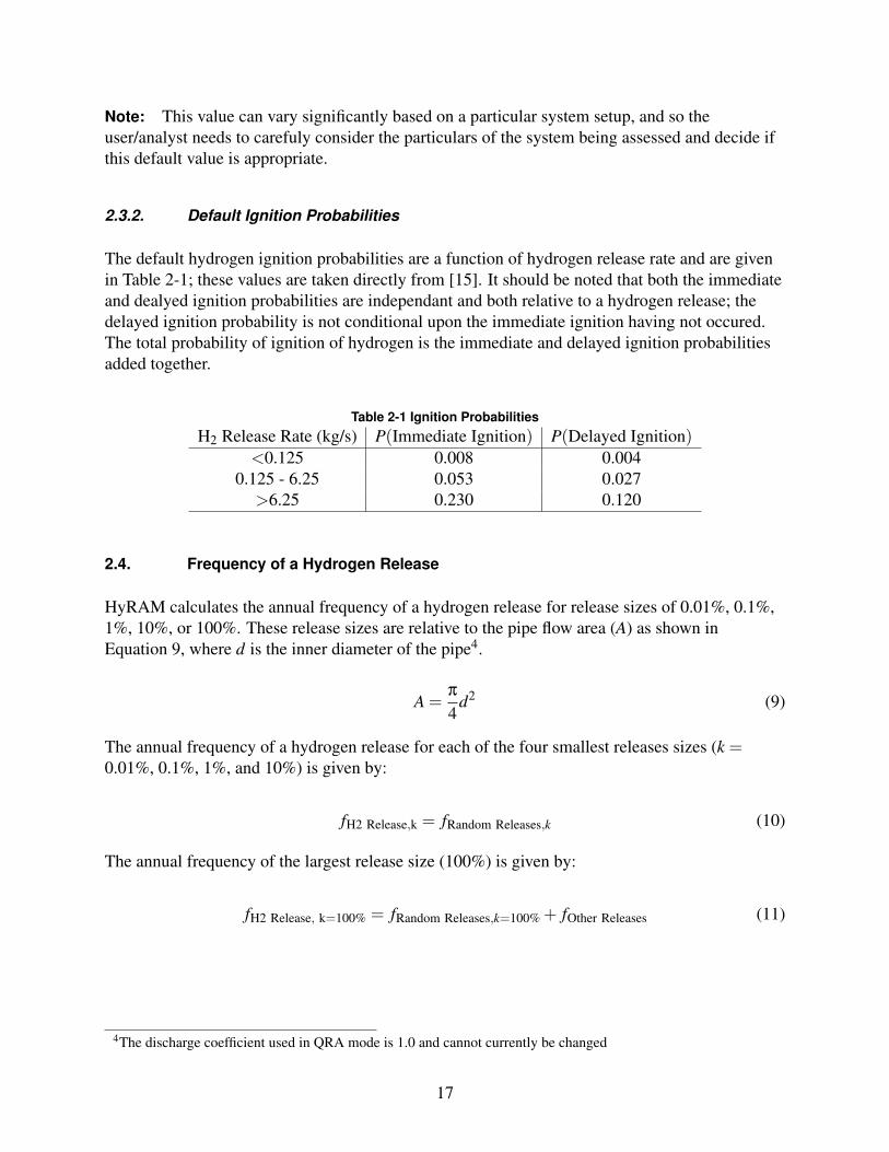
2.4.1. Frequency of Random Leaks

The annual frequency of random leaks is obtained for each release size using a fault tree. As anexample, the fault tree for random leaks for leak size 0.01% is shown in Figure 2-3. The faulttrees for random leaks for all other leak sizes are analagous per leak size.

Figure 2-3 Fault tree for random leaks of size 0.01% from H2 components

The fault trees are encoded in HyRAM to combine component leak frequencies into an overallleak frequency for each size. The annual frequency of random leaks ( fRandom Releases,k) iscalculated for each release of size k by combining the individual component leak frequencies forall the components in the system of interest:

fRandom Releases,k = ∑i

NComponenti× fLeaki,k (12)

where NComponenti is the number of components of each type and fLeaki,k is the mean leakfrequency of size k for component i (see Section 2.4.2). The component types are Compressors,Cylinders, Filters, Flanges, Hoses, Joints, Pipes (1 m)5, Valves, Instruments, Extra Component#1, and Extra Component #2.

2.4.2. Default Component Leak Frequencies

In HyRAM, the annual frequency of a random leak ( fLeak) is assumed to be distributed as alognormal distribution with parameters µ and σ:

fLeak ∼ Lognormal(µ,σ2) (13)

For a lognormal distribution, the arithmetic mean is given by:

5The "Pipes (1 m)" component type is per-meter of pipe; so if a system has 15 m worth of piping, then the "number"of components for that type is 15.

18

mean = eµ+σ2/2 (14)

The geometric mean (which is equal to the median) is given by:

median = eµ (15)

The lognormal distribution is not symmetric on a linear scale and can cover multiple orders ofmagnitude, which can lead to unrealistically high values for the arithmetic mean. Therefore, thegeometric mean (median) will be used in the frequency calcualtions in HyRAM as a moreconsistant metric of central-tendency for the distribution.

The default values are generic hydrogen-system leak frequencies developed by LaChance etal. [4]. A numerical curve-fit was done in order to obtain values for lognormal distributionparameters (µ, σ) that fit the reported values in that report6. The resulting parameters (µ, σ)obtained by this curve-fit, as well as the resulting values for arithmetic mean, geometric mean(median), 5th percentile, and 95th percentile values are found in Table 2-2.

In HyRAM 3.1, only the geometric mean (median) leak frequency is used in release calculationsbased on lognormal distributions. Future versions of HyRAM may be designed to use additionalinformation from the lognormal distribution in uncertainty propagation.

The leak frequency values for the "Instruments" component are not reported in LaChance etal. [4], but are reported in a previous analysis by Groth et al. [8]. However, the curve-fitperformed is different than the method the previous analysis used, leading to slightly differentparameter values (for all components, not just Instruments).

The component types Extra Component #1 and Extra Component #2 were added as optionalplaceholder components that might not fall into the other component type categories. Theintention is that users can specify a custom leak frequency distribution for these componentswhile still keeping the leak frequency distributions for the other components. The default leakfrequency distribution parameters (µ, σ) for these components are 0.0, since this is meant to beedited by the user.

6Specifically, a 3-point curve fit was performed based on the 5th, 50th (median), and 95th values provided in LaChanceet al. [4] using a least-squares solver method in the SciPy library

19

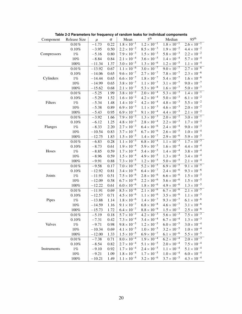
Table 2-2 Parameters for frequency of random leaks for individual componentsComponent Release Size µ σ Mean 5th Median 95th

Compressors

0.01% −1.73 0.22 1.8×10−1 1.2×10−1 1.8×10−1 2.6×10−1

0.10% −3.95 0.50 2.2×10−2 8.5×10−3 1.9×10−2 4.4×10−2

1% −5.16 0.80 7.9×10−3 1.5×10−3 5.8×10−3 2.2×10−2

10% −8.84 0.84 2.1×10−4 3.6×10−5 1.4×10−4 5.7×10−4

100% −11.34 1.37 3.0×10−5 1.3×10−6 1.2×10−5 1.1×10−4

Cylinders

0.01% −13.92 0.67 1.1×10−6 3.0×10−7 9.0×10−7 2.7×10−6

0.10% −14.06 0.65 9.6×10−7 2.7×10−7 7.8×10−7 2.3×10−6

1% −14.44 0.65 6.6×10−7 1.8×10−7 5.4×10−7 1.6×10−6

10% −14.99 0.65 3.8×10−7 1.1×10−7 3.1×10−7 9.0×10−7

100% −15.62 0.68 2.1×10−7 5.3×10−8 1.6×10−7 5.0×10−7

Filters

0.01% −5.25 1.99 3.8×10−2 2.0×10−4 5.3×10−3 1.4×10−1

0.10% −5.29 1.52 1.6×10−2 4.2×10−4 5.0×10−3 6.1×10−2

1% −5.34 1.48 1.4×10−2 4.2×10−4 4.8×10−3 5.5×10−2

10% −5.38 0.89 6.9×10−3 1.1×10−3 4.6×10−3 2.0×10−2

100% −5.43 0.95 6.9×10−3 9.1×10−4 4.4×10−3 2.1×10−2

Flanges

0.01% −3.92 1.66 7.9×10−2 1.3×10−3 2.0×10−2 3.0×10−1

0.10% −6.12 1.25 4.8×10−3 2.8×10−4 2.2×10−3 1.7×10−2

1% −8.33 2.20 2.7×10−3 6.4×10−6 2.4×10−4 9.0×10−3

10% −10.54 0.83 3.7×10−5 6.7×10−6 2.6×10−5 1.0×10−4

100% −12.75 1.83 1.5×10−5 1.4×10−7 2.9×10−6 5.9×10−5

Hoses

0.01% −6.83 0.28 1.1×10−3 6.8×10−4 1.1×10−3 1.7×10−3

0.10% −8.73 0.61 1.9×10−4 5.9×10−5 1.6×10−4 4.4×10−4

1% −8.85 0.59 1.7×10−4 5.4×10−5 1.4×10−4 3.8×10−4

10% −8.96 0.59 1.5×10−4 4.9×10−5 1.3×10−4 3.4×10−4

100% −9.91 0.88 7.3×10−5 1.2×10−5 5.0×10−5 2.1×10−4

Joints

0.01% −9.58 0.17 7.0×10−5 5.2×10−5 6.9×10−5 9.1×10−5

0.10% −12.92 0.81 3.4×10−6 6.4×10−7 2.4×10−6 9.3×10−6

1% −11.93 0.51 7.5×10−6 2.8×10−6 6.6×10−6 1.5×10−5

10% −12.09 0.58 6.7×10−6 2.2×10−6 5.6×10−6 1.5×10−5

100% −12.22 0.61 6.0×10−6 1.8×10−6 4.9×10−6 1.3×10−5

Pipes

0.01% −11.91 0.69 8.5×10−6 2.1×10−6 6.7×10−6 2.1×10−5

0.10% −12.57 0.71 4.5×10−6 1.1×10−6 3.5×10−6 1.1×10−5

1% −13.88 1.14 1.8×10−6 1.4×10−7 9.3×10−7 6.1×10−6

10% −14.59 1.16 9.1×10−7 6.8×10−8 4.6×10−7 3.1×10−6

100% −15.73 1.72 6.4×10−7 8.8×10−9 1.5×10−7 2.5×10−6

Valves

0.01% −5.19 0.18 5.7×10−3 4.2×10−3 5.6×10−3 7.5×10−3

0.10% −7.31 0.42 7.3×10−4 3.4×10−4 6.7×10−4 1.3×10−3

1% −9.71 0.98 9.8×10−5 1.2×10−5 6.0×10−5 3.0×10−4

10% −10.34 0.69 4.1×10−5 1.0×10−5 3.2×10−5 1.0×10−4

100% −12.00 1.33 1.5×10−5 6.9×10−7 6.1×10−6 5.5×10−5

Instruments

0.01% −7.38 0.71 8.0×10−4 1.9×10−4 6.2×10−4 2.0×10−3

0.10% −8.54 0.82 2.7×10−4 5.1×10−5 2.0×10−4 7.5×10−4

1% −9.10 0.92 1.7×10−4 2.4×10−5 1.1×10−4 5.1×10−4

10% −9.21 1.09 1.8×10−4 1.7×10−5 1.0×10−4 6.0×10−4

100% −10.21 1.49 1.1×10−4 3.2×10−6 3.7×10−5 4.3×10−4

20

2.4.3. Frequency of Dispenser Releases

The annual frequency of other releases ( fOther Releases) deals with failures that can happen at adispenser, rather than random leaks from individual components. In addition to random leaks thatcan develop from any component at any time, there is also the possibility of a release occuringdue to some component failure or accident while fueling. Fueling typically involves direct humaninteraction to operate the fueling dispenser, involves temporary connections rather thanhard-plumbed lines, and the vehicle is not a permanent part of the system and so mayinadvertently break the connection. On the other hand, releases from fueling can only occur whenfueling occurs, and so different systems that involve different number of fueling events can beimpacted by these releases to varying degrees. It is assumed that a dispenser failure would resultin a large release of hydrogen, and so this frequency is only used in the largest (100%) leak size.The annual frequency of other releases ( fOther Releases) is calculated by the following equation:

fOther Releases = fFueling Demands×P(Dispenser Releases) (16)

where fFueling Demands is the annual frequency of fueling demands (i.e., the number of times adispenser is used to refuel a vehicle in a year) and P(Dispenser Releases) is the probability of arelease from a dispenser during fueling. The annual frequency of fueling demands is given by:

fFueling Demands = NVehicles×NFuelings per Day×NOperating Days per Year (17)

where NVehicles is the number of vehicles at the facility, NFuelings per Day is the average number oftimes each vehicle is fueled per day, and NOperating Days per Year is the number of operating days ina year.

Dispenser failures are categorized in HyRAM as Accidents (in which the vehicle tankoverpressurizes or a drive-off occurs) or Shutdown Failures (in which the system failures to shutdown after a release from the nozzle). The probability for these types of releases are determinedby a fault tree as shown in Figure 2-4.

21

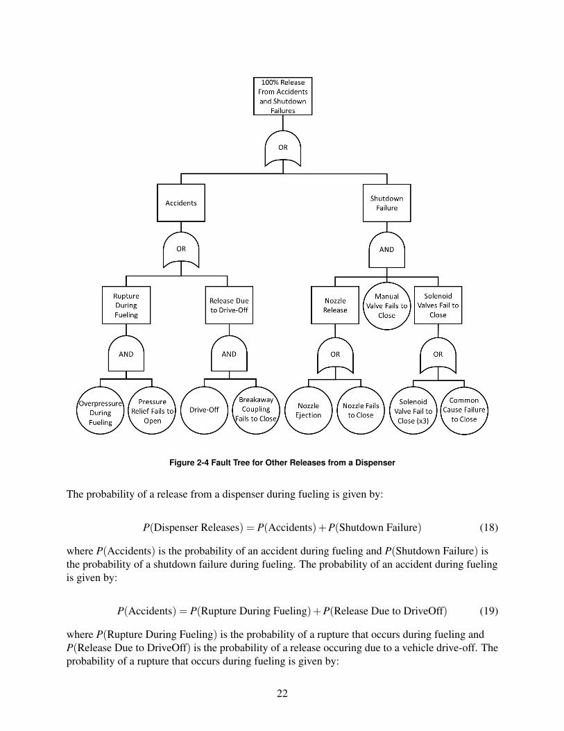
Figure 2-4 Fault Tree for Other Releases from a Dispenser

The probability of a release from a dispenser during fueling is given by:

P(Dispenser Releases) = P(Accidents)+P(Shutdown Failure) (18)

where P(Accidents) is the probability of an accident during fueling and P(Shutdown Failure) isthe probability of a shutdown failure during fueling. The probability of an accident during fuelingis given by:

P(Accidents) = P(Rupture During Fueling)+P(Release Due to DriveOff) (19)

where P(Rupture During Fueling) is the probability of a rupture that occurs during fueling andP(Release Due to DriveOff) is the probability of a release occuring due to a vehicle drive-off. Theprobability of a rupture that occurs during fueling is given by:

22

P(Rupture During Fueling) = P(Overpressure During Fueling)×P(PRD FTO) (20)

where P(Overpressure During Fueling) is the probability of an overpressure occuring duringfueling (e.g., the dispenser over-fills the vehicle tank) and P(PRD FTO) is the probability of thedispenser pressure relief device failing to open on demand. The probabilitiesP(Overpressure During Fueling) and P(PRD FTO) can each be specified as a specific expectedvalue from 0.0 to 1.0, or can be specified as a probability distribution such as Beta or Log-Normaldistributions. If a probability distribution is specified, the mean value will be calculated and usedin the above calculations. Default values for these probabilities are given in Section 2.4.4.

The probability of a release occuring due to a vehicle drive-off is given by:

P(Release Due to DriveOff) = P(DriveOff)×P(Breakaway FTC) (21)

where P(DriveOff) is the probability of a vehicle driving off while still attached to the dispenserduring fueling and P(Breakaway FTC) is the probability of the breakaway coupling failing toclose on demand. The probabilities P(DriveOff) and P(Breakaway FTC) can each be specified asa specific expected value from 0.0 to 1.0, or can be specified as a probability distribution such asBeta or Log-Normal distributions. If a probability distribution is specified, the mean value will becalculated and used in the above calculations. Default values for these probabilities are given inSection 2.4.4.

The probability a shutdown failure during fueling is given by:

P(Shutdown Failure) = P(Nozzle Release)×P(Manual Valve FTC)×P(Solenoid Valves FTC)(22)

where P(Nozzle Release) is the probability of the dispensing nozzle releasing hydrogen,P(Manual Valve FTC) is the probability of the manual shutoff valve failing to close on demand,and P(Solenoid Valves FTC) is the probability of the automated solenoid valves on the dispenserfailing to close on demand. The probability of the manual shutoff valve failing to close ondemand (P(Manual Valve FTC)) can be specified as a specific expected value or can be specifiedas a probability distribution (Beta or Log-Normal) for which the mean value will be used. Defaultvalues for this probability are given in Section 2.4.4.

The probability of the dispensing nozzle releasing hydrogen is given by:

P(Nozzle Release) = P(Nozzle Ejection)+P(Nozzle FTC) (23)

where P(Nozzle Ejection) is the probability of the dispenser nozzle being ejected during fueling,and P(Nozzle FTC) is the probability of the dispenser nozzle failing to close on demand. Theseprobabilities P(Nozzle Ejection) and P(Nozzle FTC) can each be specified as a specific expectedvalue or can be specified as a probability distribution (Beta or Log-Normal) for which the meanvalue will be used. Default values for this probability are given in Section 2.4.4.

23

The probability of the automated solenoid valves on the dispenser failing to close on demand isgiven by:

P(Solenoid Valves FTC) = [P(Solenoid Valve FTC)]3 +P(Common Cause FTC) (24)

where P(Solenoid Valve FTC) is the probability of any one automated solenoid valve failing toclose on demand and P(Common Cause FTC) is the probability of something causing all of thesolenoid valves to fail to close on demand (e.g., loss of connection to sensors). It should be notedthat this fault tree assumes that there are 3 solenoid valves and that all of them need to fail in orderfor hydrogen to be released; thus, the probability for any single valve is cubed. These probabilitiesP(Solenoid Valve FTC) and P(Common Cause FTC) can each be specified as a specific expectedvalue or can be specified as a probability distribution (Beta or Log-Normal) for which the meanvalue will be used. Default values for this probability are given in Section 2.4.4.

It should be noted that any of the probabilities in this section can be used to estimate an annualfrequency of how often any of the events in question are expected to happen in a year. This can bedone by multiplying the probability of interest (P(A)) by the annual number of fueling demands( fFueling Demands) for some event A:

fA = P(A)× fFueling Demands (25)

2.4.4. Default Dispenser Failure Probabilities

In HyRAM 3.1, only the geometric mean (median) leak frequency is used in release calculationsfor the lognormal distributions and the arithmetic mean is used for the beta distributions. Futureversions of HyRAM may be designed to use additional information from these distributions inuncertainty propagation.

See Section 2.4.2 for the calculation of the mean for a lognormal distribution. For a betadistribution with parameters α and β, the arithmetic mean is given by:

mean =α

α+β(26)

The default failure probabilities in this section were assembled from generic data from theoffshore oil, process chemical, and nuclear power industries, and are taken directly from Ref[8].

24

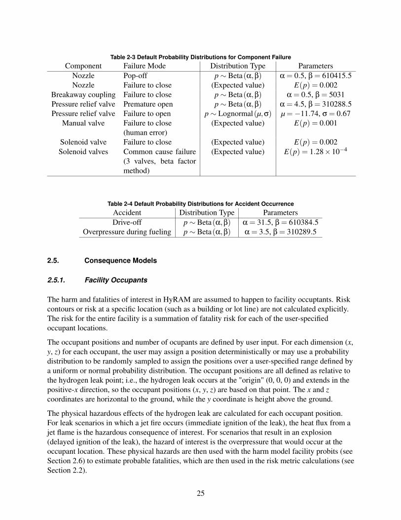
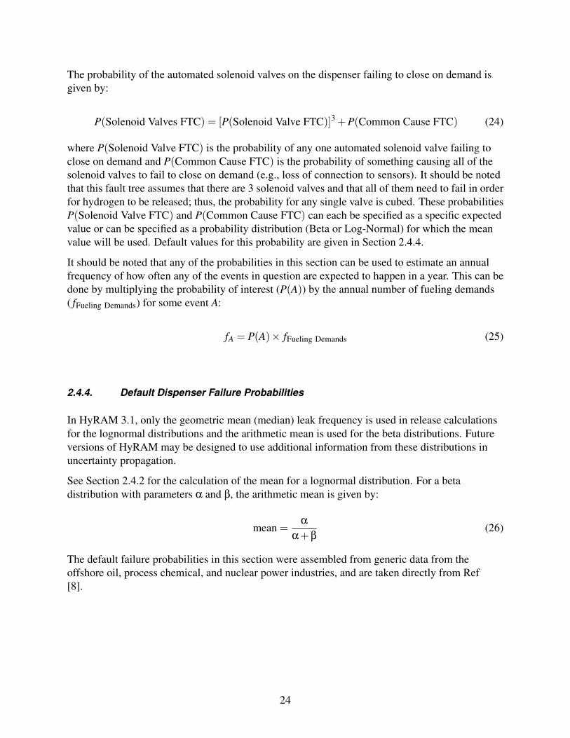
Table 2-3 Default Probability Distributions for Component FailureComponent Failure Mode Distribution Type Parameters

Nozzle Pop-off p∼ Beta(α,β) α = 0.5, β = 610415.5Nozzle Failure to close (Expected value) E(p) = 0.002

Breakaway coupling Failure to close p∼ Beta(α,β) α = 0.5, β = 5031Pressure relief valve Premature open p∼ Beta(α,β) α = 4.5, β = 310288.5Pressure relief valve Failure to open p∼ Lognormal(µ,σ) µ =−11.74, σ = 0.67

Manual valve Failure to close(human error)

(Expected value) E(p) = 0.001

Solenoid valve Failure to close (Expected value) E(p) = 0.002Solenoid valves Common cause failure

(3 valves, beta factormethod)

(Expected value) E(p) = 1.28×10−4

Table 2-4 Default Probability Distributions for Accident OccurrenceAccident Distribution Type ParametersDrive-off p∼ Beta(α,β) α = 31.5, β = 610384.5

Overpressure during fueling p∼ Beta(α,β) α = 3.5, β = 310289.5

2.5. Consequence Models

2.5.1. Facility Occupants

The harm and fatalities of interest in HyRAM are assumed to happen to facility occuptants. Riskcontours or risk at a specific location (such as a building or lot line) are not calculated explicitly.The risk for the entire facility is a summation of fatality risk for each of the user-specifiedoccupant locations.

The occupant positions and number of ocupants are defined by user input. For each dimension (x,y, z) for each occupant, the user may assign a position deterministically or may use a probabilitydistribution to be randomly sampled to assign the positions over a user-specified range defined bya uniform or normal probability distribution. The occupant positions are all defined as relative tothe hydrogen leak point; i.e., the hydrogen leak occurs at the "origin" (0, 0, 0) and extends in thepositive-x direction, so the occupant positions (x, y, z) are based on that point. The x and zcoordinates are horizontal to the ground, while the y coordinate is height above the ground.

The physical hazardous effects of the hydrogen leak are calculated for each occupant position.For leak scenarios in which a jet fire occurs (immediate ignition of the leak), the heat flux from ajet flame is the hazardous consequence of interest. For scenarios that result in an explosion(delayed ignition of the leak), the hazard of interest is the overpressure that would occur at theoccupant location. These physical hazards are then used with the harm model facility probits (seeSection 2.6) to estimate probable fatalities, which are then used in the risk metric calculations (seeSection 2.2).

25

2.5.2. Jet Fire

The consequences of a jet fire (for each of the five release sizes) on facility occupants arecalculated using the models described in Section 3. Users can select the straight-flame model ofHouf and Schefer [26] as described in Section 3.4.2, or the curved-flame model from Ekoto etal. [27] as described in Section 3.4.3. Both of these models are coupled to the orifice flow andnotional nozzle models described in Section 3.3. The discharge coefficient Cd is set to 1.0 for theQRA calculations. The heat flux calculation is performed at each of the occupant locations.

2.5.3. Explosion (Deflagration or Detonation) Overpressure

Users must input the peak overpressure and impulse values for the five release sizes. These valuescan come from calculations using computational simulation, first-order models, or engineeringassumptions. These values are then applied to all facility occupants. Subsequent versions ofHyRAM will improve the treatment of overpressure per occupant and will allow a way toestimate overpressure and impulse values directly, similar to how heat flux thermal hazards areestimated.

2.5.4. Default Overpressure and Impulse Values

Currently, HyRAM uses a set of peak overpressure and impulse values as the default for delayedignition scenarios; these values are editable by the user. The peak overpressure and impulse areused with the overpressure harm models in Section 2.6.2. The default peak overpressure valuesgiven in HyRAM are taken from numerical simulations performed for a warehouse withhydrogen-powered forklifts [8]. These simulations calculated peak overpressure values for the100%, 10%, and 1% leak sizes; the smaller leak sizes (0.1% and 0.01%) used half of the peakoverpressure as the 1% leak size. Default values for impulse are taken from the same simulations[8], which estimated the impulse for the largest leak size (100%) and assumed that smaller leaksproduce half of the impulse as the next-largest leak. The default peak overpressure and impulsevalues in HyRAM are given in Table 2-5.

Table 2-5 Peak Overpressure and Impulse ValuesLeak Size Peak Overpressure (Pa) Impulse (Pa·s)

0.01% 2500 2500.1% 2500 5001% 5000 1000

10% 16000 2000100% 30000 4000

26

2.6. Harm and Loss Models

Probit models are used to establish the probability of injury or fatality for a given exposure. Theprobit model is a linear combination of predictors that model the inverse cumulative distributionfunction associated with the normal distribution7. The probability of a fatality is given byEquation 27, which evaluates the normal cumulative distribution function, Φ, at the valueestablished by the appropriate probit model (Y , see Sections 2.6.1 and 2.6.2).

P(fatality) = F(Y |µ = 5,σ = 1) = Φ(Y −5) (27)

2.6.1. Thermal Harm

For thermal radiation, the harm level is a function of both the heat flux intensity and the durationof exposure. Harm from radiant heat fluxes is often expressed in terms of a thermal dose unit (V )which combines the heat flux intensity and exposure time by Equation 28:

V = I(4/3)× t (28)

where I is the radiant heat flux in W/m2 and t is the exposure duration in seconds. The defaultthermal exposure time used in HyRAM is 60 s, but users may modify this value.

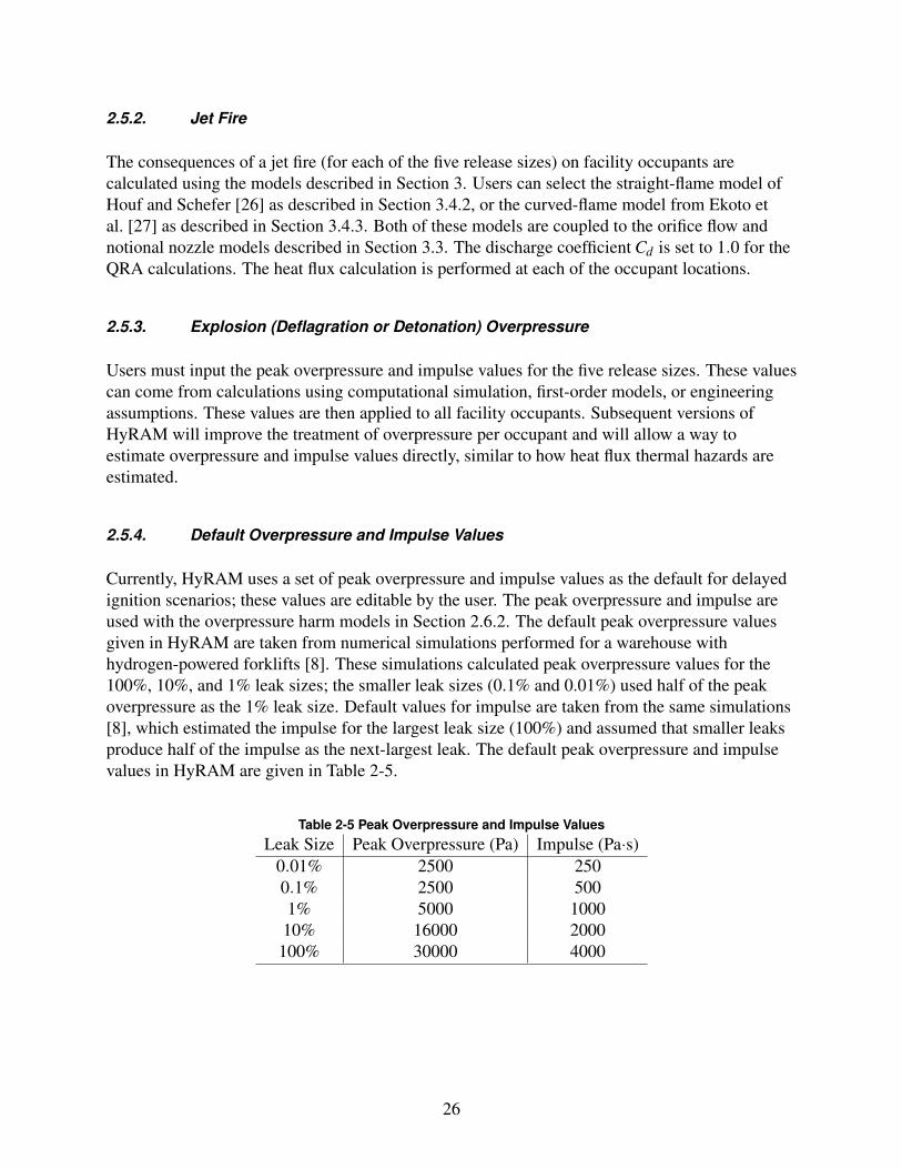
Table 2-6 lists five thermal probit models that are encoded in HyRAM. The probability of afatality is evaluated by inserting the probit model from Table 2-6 into Equation 27. LaChance etal. [28] recommend using both the Eisenberg and the Tsao & Perry probit models forhydrogen-related applications.

Table 2-6 Probit models used to calculate fatality probability as a function of thermal dose (V )

Reference Fatality Model NotesEisenberg [29] Y =−38.48+2.56× ln(V ) Based on population data from nuclear

blasts at Hiroshima and Nagasaki (ultra-violet radiation)

Tsao & Perry [30] Y =−36.38+2.56× ln(V ) Eisenberg model, modified to accountfor infrared radiation

TNO [31] Y =−37.23+2.56× ln(V ) Tsao and Perry model modified to ac-count for clothing

Lees [32] Y =−29.02+1.99× ln(0.5V ) Accounts for clothing, based on porcineskin experiments using ultravioletsource to determine skin damages.Uses burn mortality information.

7Today, probit model are associated with the standard normal distribution, with mean µ = 0 and standard deviationσ = 1. Some older probit models were developed using µ = 5 to avoid negative values. HyRAM uses µ = 5 to beconsistent with the published fatality probit models.

27

Structures and equipment can also be damaged by exposure to radiant heat flux. Some typicalheat flux values and exposure times for damage to structures and components were provided byLaChance et al. [28]. However, because the exposure times required for damage is long(>30 min), the impact of thermal radiation from hydrogen fires on structures and equipment isnot generally significant since personnel are able to evacuate the building before significantstructural damage occurs. This is only noted because structural damage can cause physical harm(fatalaties) to humans, which is the risk metric of interest within HyRAM.

2.6.2. Overpressure Harm

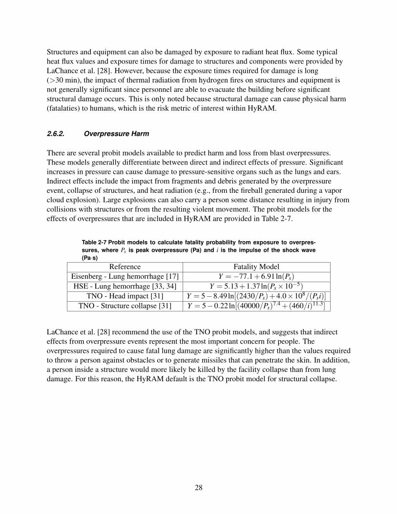
There are several probit models available to predict harm and loss from blast overpressures.These models generally differentiate between direct and indirect effects of pressure. Significantincreases in pressure can cause damage to pressure-sensitive organs such as the lungs and ears.Indirect effects include the impact from fragments and debris generated by the overpressureevent, collapse of structures, and heat radiation (e.g., from the fireball generated during a vaporcloud explosion). Large explosions can also carry a person some distance resulting in injury fromcollisions with structures or from the resulting violent movement. The probit models for theeffects of overpressures that are included in HyRAM are provided in Table 2-7.

Table 2-7 Probit models to calculate fatality probability from exposure to overpres-sures, where Ps is peak overpressure (Pa) and i is the impulse of the shock wave(Pa·s)

Reference Fatality ModelEisenberg - Lung hemorrhage [17] Y =−77.1+6.91ln(Ps)

HSE - Lung hemorrhage [33, 34] Y = 5.13+1.37ln(Ps×10−5)

TNO - Head impact [31] Y = 5−8.49ln[(2430/Ps)+4.0×108/(Psi)]TNO - Structure collapse [31] Y = 5−0.22ln[(40000/Ps)

7.4 +(460/i)11.3]

LaChance et al. [28] recommend the use of the TNO probit models, and suggests that indirecteffects from overpressure events represent the most important concern for people. Theoverpressures required to cause fatal lung damage are significantly higher than the values requiredto throw a person against obstacles or to generate missiles that can penetrate the skin. In addition,a person inside a structure would more likely be killed by the facility collapse than from lungdamage. For this reason, the HyRAM default is the TNO probit model for structural collapse.

28

3. PHYSICS MODELS

HyRAM includes a physics mode, which provides models relevant to modeling behavior, hazards,and consequences of hydrogen releases. Jet flames, concentration profiles for unignitedjets/plumes, and indoor accumulation with delayed ignition causing overpressure can all beinvestigated from the physics mode. A subset of these models is used in the QRA mode tocalculate the consequences from a given release scenario, as described in Section 2.5. Severalbasic property calculations (e.g., the thermodynamic equation of state for hydrogen) are necessaryto numerically simulate hydrogen release scenarios, and these property calculations are used inother models.

3.1. Properties of Hydrogen

The modules in this section provide thermodynamic properties of unignited and ignited hydrogen,which are needed to calculate different aspects of hydrogen dispersion and combustion. Thesecalculations are called from several of the other models. They are described here in detail, andthen referred to in subsequent sections.

3.1.1. Equation of State

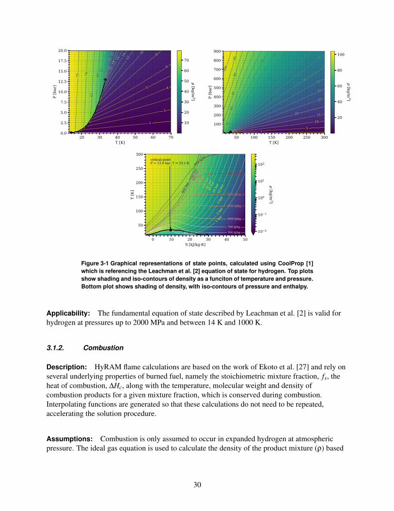
Description: HyRAM 3.1 utilizes the CoolProp library [1], called through its Python interfaceto perform several thermodynamic calculations. The property calculations are based on aHelmholtz energy function, and account for the real gas behavior at high pressures and atcryogenic temperatures. CoolProp can be used to calculate the properties of hydrogen, air or othergases. For hydrogen, the relationships are detailed in Leachman et al. [2]. These thermodynamiccalculations are used to calculate leak rates and are used in mass, momentum, and energybalances in regions close to the leak point. The relationships between pressure8, temperature,density, enthalpy, and entropy are plotted in Figure 3-1. In some regions of the models, the idealgas equation of state is used, as described in other sections.

8HyRAM calculation inputs use absolute pressure, not gauge pressure

29

20 30 40 50 60 70T [K]

0.0

2.5

5.0

7.5

10.0

12.5

15.0

17.5

20.0P

[bar

]

1

2

3

45

6

810

1214

1618

2025

3035

4045

5055

60

657075

10

20

30

40

50

60

70

[kg/m3]

50 100 150 200 250 300T [K]

100

200

300

400

500

600

700

800

900

P [b

ar]

15

10

1520

25

30

3540

4550

55

6065

70

7580

8590

95

100

20

40

60

80

100

[kg/m3]

0 10 20 30 40 50S [kJ/kg-K]

50

100

150

200

250

300

T [K

]

critical pointP = 13.0 bar, T = 33.1 K

1 bar

2 ba

r5

bar

10 b

ar

20 b

ar

40 b

ar

60 b

ar

100

bar

200

bar

300

bar

500

bar

700

bar

900

bar

300 kJ/kg400 kJ/kg 500 kJ/kg

700 kJ/kg

1000 kJ/kg

1500 kJ/kg

2000 kJ/kg

3000 kJ/kg

4000 kJ/kg

10 2

10 1

100

101

102

[kg/m3]

Figure 3-1 Graphical representations of state points, calculated using CoolProp [1]which is referencing the Leachman et al. [2] equation of state for hydrogen. Top plotsshow shading and iso-contours of density as a funciton of temperature and pressure.Bottom plot shows shading of density, with iso-contours of pressure and enthalpy.

Applicability: The fundamental equation of state described by Leachman et al. [2] is valid forhydrogen at pressures up to 2000 MPa and between 14 K and 1000 K.

3.1.2. Combustion

Description: HyRAM flame calculations are based on the work of Ekoto et al. [27] and rely onseveral underlying properties of burned fuel, namely the stoichiometric mixture fraction, fs, theheat of combustion, ∆Hc, along with the temperature, molecular weight and density ofcombustion products for a given mixture fraction, which is conserved during combustion.Interpolating functions are generated so that these calculations do not need to be repeated,accelerating the solution procedure.

Assumptions: Combustion is only assumed to occur in expanded hydrogen at atmosphericpressure. The ideal gas equation is used to calculate the density of the product mixture (ρ) based

30

on the molecular weight of the mixture (MWmixture), the temperature (T ), and the gas constant(R):

ρ =P(MWmixture)

RT(29)

These combustion calculations assume that there are no losses, that the mixture is thermallyperfect with the local enthalpy, and the pressure of the products is the same as the pressure of thereactants.

Relationships: Stoichiometric combustion of hydrogen in air (ignoring the minor species inair) can be written as

H2 +12(O2 +3.76N2)→ H2O(g)+1.88N2 +242kJ/molH2 (30)

As shown in this equation, the heat of combustion for hydrogen is 242 kJ/molH2 or 120 MJ/kgH2

(using the lower heating value) [35, 36]. From this equation, the stoichiometric mixture fraction( fs), which is the same as the mass fraction of hydrogen, can be calculated as:

fs =MWH2

MWH2 +0.5(MWO2 +3.76MWN2)=

MWH2

MWH2O +1.88MWN2

= 0.02852 (31)

If incomplete combustion occurs (a mixture fraction other than stoichiometric), there will beexcess air or hydrogen on the right hand side of Equation 30 at the temperature of the productstream. In other words,

H2 +η

2(O2 +3.76N2)→max(0,1−η)H2 +min(1,η)H2O+max

(0,

η−12

)O2 +3.76

η

2N2,

(32)

where η can vary from 0 to ∞. In this case, the mixture fraction is equal to

f =MWH2(xH2 + xH2O)

MW= YH2 +YH2O

MWH2

MWH2O(33)

where x is the mole fraction and Y is the mass fraction of products or reactants. HyRAM usesCoolProp [1] to look up the enthalpy of H2, H2O, O2, and N2 as interpolating functions oftemperature and then solves for the temperature of products assuming an isenthalpic reaction,i.e.,

31

∑i=H2,O2,N2

Yi,reachi,reac(Treac,Preac) = ∑i=H2,O2,N2,H2O

Yi,prodhi,prod(Tprod,Pprod)+YH2O,prodMWH2

MWH2O∆Hc

(34)

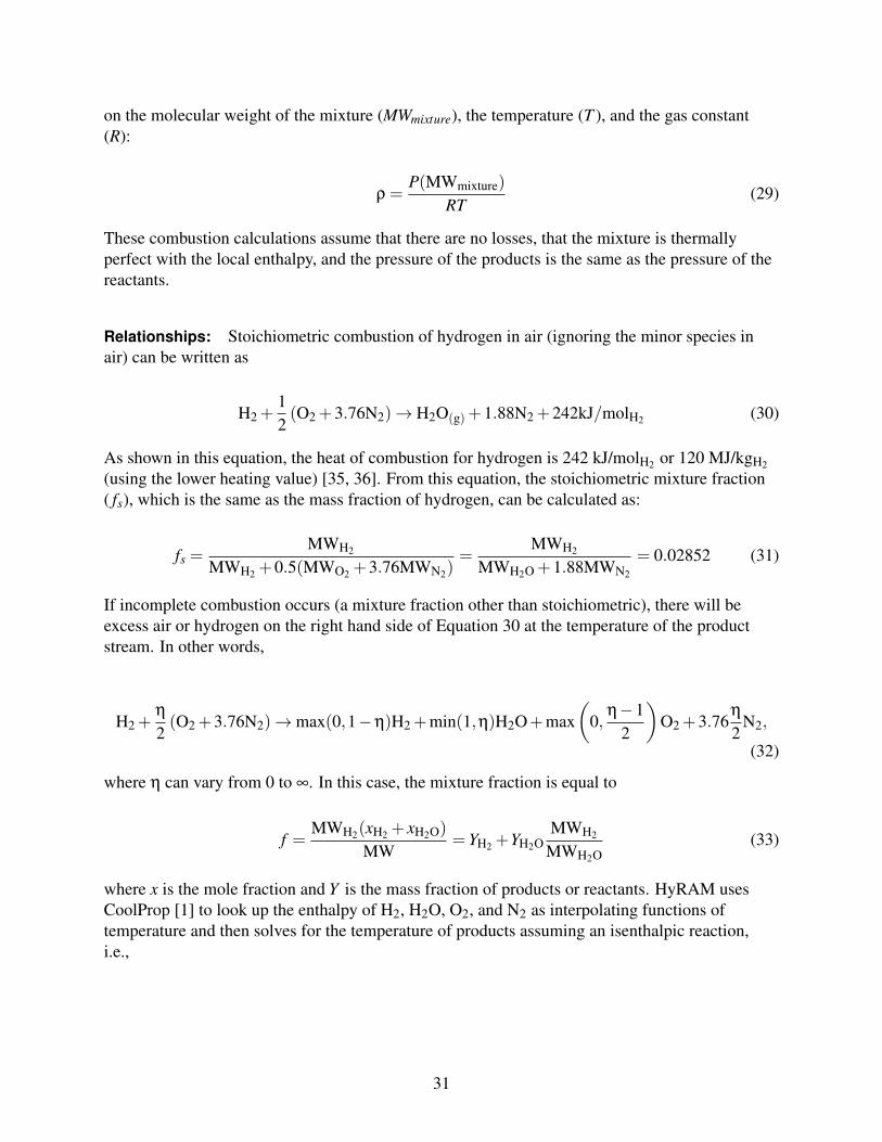
The calculation of the adiabatic flame temperature (Tad) and density of the products of 298 K,101,325 Pa hydrogen are shown in Figure 3-2.

500

1000

1500

2000

T pro

duct

s [K

]

Tfs = 2214 K

f s=

0.02

852

0.0 0.2 0.4 0.6 0.8 1.0mixture fraction (fs)

0.25

0.50

0.75

1.00

prod

uctm

ixtu

re (k

g/m

3 )

f s=

0.02

852

Figure 3-2 Temperature and density of products for the combustion of 298 K,101,325 Pa hydrogen as a function of mixture fraction

Applicability: These combustion calculations are applicable in atmospheric pressure regionswhere heat losses are negligible.

3.2. Developing Flow

Several engineering models are used in HyRAM to establish the flow through an orifice, expandto atmospheric pressure, warm to a level that the equation of state is valid, and develop into theGaussian profiles that are well known for jet/plume dispersion or diffusion flames.

3.2.1. Orifice Flow

HyRAM assumes that gases flow isentropically through an orifice. CoolProp [1] is used tocalculate the entropy (s0) and enthalpy (h0) of the fluid upstream of an orifice, using the specifiedpressure and temperature (or phase if a saturated vapor or saturated liquid is specified). CoolPropis then used to calculate the enthalpy (h), temperature (T ), and sonic velocity (a) of a fluid at

32

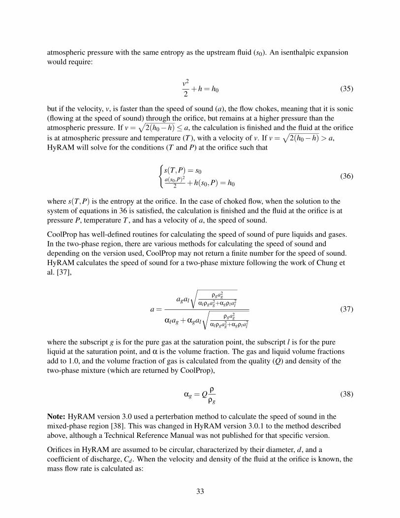
atmospheric pressure with the same entropy as the upstream fluid (s0). An isenthalpic expansionwould require:

v2

2+h = h0 (35)

but if the velocity, v, is faster than the speed of sound (a), the flow chokes, meaning that it is sonic(flowing at the speed of sound) through the orifice, but remains at a higher pressure than theatmospheric pressure. If v =

√2(h0−h)≤ a, the calculation is finished and the fluid at the orifice

is at atmospheric pressure and temperature (T ), with a velocity of v. If v =√

2(h0−h)> a,HyRAM will solve for the conditions (T and P) at the orifice such that

{s(T,P) = s0a(s0,P)2

2 +h(s0,P) = h0(36)

where s(T,P) is the entropy at the orifice. In the case of choked flow, when the solution to thesystem of equations in 36 is satisfied, the calculation is finished and the fluid at the orifice is atpressure P, temperature T , and has a velocity of a, the speed of sound.

CoolProp has well-defined routines for calculating the speed of sound of pure liquids and gases.In the two-phase region, there are various methods for calculating the speed of sound anddepending on the version used, CoolProp may not return a finite number for the speed of sound.HyRAM calculates the speed of sound for a two-phase mixture following the work of Chung etal. [37],

a =

agal

√ρga2

g

αlρga2g+αgρla2

l

αlag +αgal

√ρga2

g

αlρga2g+αgρla2

l

(37)

where the subscript g is for the pure gas at the saturation point, the subscript l is for the pureliquid at the saturation point, and α is the volume fraction. The gas and liquid volume fractionsadd to 1.0, and the volume fraction of gas is calculated from the quality (Q) and density of thetwo-phase mixture (which are returned by CoolProp),

αg = Qρ

ρg(38)

Note: HyRAM version 3.0 used a perterbation method to calculate the speed of sound in themixed-phase region [38]. This was changed in HyRAM version 3.0.1 to the method describedabove, although a Technical Reference Manual was not published for that specific version.

Orifices in HyRAM are assumed to be circular, characterized by their diameter, d, and acoefficient of discharge, Cd . When the velocity and density of the fluid at the orifice is known, themass flow rate is calculated as:

33

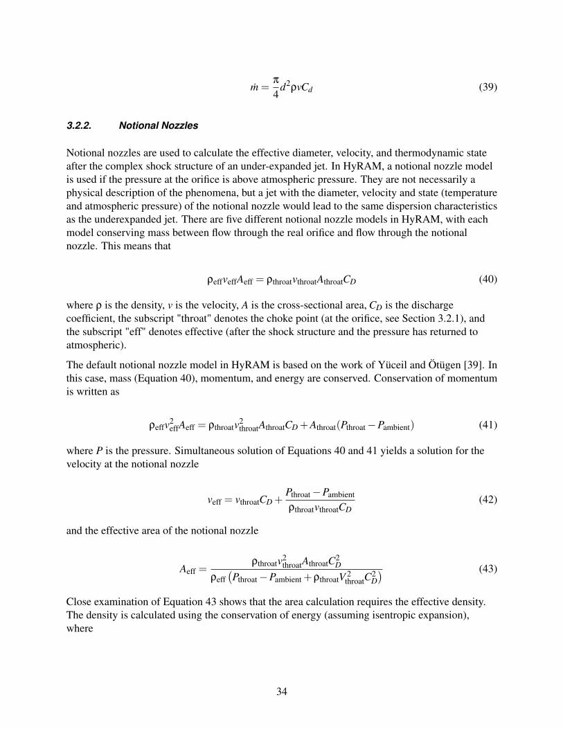
m =π

4d2

ρvCd (39)

3.2.2. Notional Nozzles

Notional nozzles are used to calculate the effective diameter, velocity, and thermodynamic stateafter the complex shock structure of an under-expanded jet. In HyRAM, a notional nozzle modelis used if the pressure at the orifice is above atmospheric pressure. They are not necessarily aphysical description of the phenomena, but a jet with the diameter, velocity and state (temperatureand atmospheric pressure) of the notional nozzle would lead to the same dispersion characteristicsas the underexpanded jet. There are five different notional nozzle models in HyRAM, with eachmodel conserving mass between flow through the real orifice and flow through the notionalnozzle. This means that

ρeffveffAeff = ρthroatvthroatAthroatCD (40)

where ρ is the density, v is the velocity, A is the cross-sectional area, CD is the dischargecoefficient, the subscript "throat" denotes the choke point (at the orifice, see Section 3.2.1), andthe subscript "eff" denotes effective (after the shock structure and the pressure has returned toatmospheric).

The default notional nozzle model in HyRAM is based on the work of Yüceil and Ötügen [39]. Inthis case, mass (Equation 40), momentum, and energy are conserved. Conservation of momentumis written as

ρeffv2effAeff = ρthroatv2

throatAthroatCD +Athroat(Pthroat−Pambient) (41)

where P is the pressure. Simultaneous solution of Equations 40 and 41 yields a solution for thevelocity at the notional nozzle

veff = vthroatCD +Pthroat−Pambient

ρthroatvthroatCD(42)

and the effective area of the notional nozzle

Aeff =ρthroatv2

throatAthroatC2D

ρeff(Pthroat−Pambient +ρthroatV 2

throatC2D) (43)

Close examination of Equation 43 shows that the area calculation requires the effective density.The density is calculated using the conservation of energy (assuming isentropic expansion),where

34

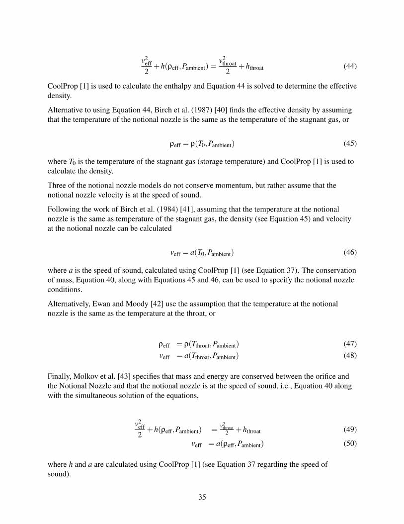
v2eff2

+h(ρeff,Pambient) =v2

throat2

+hthroat (44)

CoolProp [1] is used to calculate the enthalpy and Equation 44 is solved to determine the effectivedensity.

Alternative to using Equation 44, Birch et al. (1987) [40] finds the effective density by assumingthat the temperature of the notional nozzle is the same as the temperature of the stagnant gas, or

ρeff = ρ(T0,Pambient) (45)

where T0 is the temperature of the stagnant gas (storage temperature) and CoolProp [1] is used tocalculate the density.

Three of the notional nozzle models do not conserve momentum, but rather assume that thenotional nozzle velocity is at the speed of sound.

Following the work of Birch et al. (1984) [41], assuming that the temperature at the notionalnozzle is the same as temperature of the stagnant gas, the density (see Equation 45) and velocityat the notional nozzle can be calculated

veff = a(T0,Pambient) (46)

where a is the speed of sound, calculated using CoolProp [1] (see Equation 37). The conservationof mass, Equation 40, along with Equations 45 and 46, can be used to specify the notional nozzleconditions.

Alternatively, Ewan and Moody [42] use the assumption that the temperature at the notionalnozzle is the same as the temperature at the throat, or

ρeff = ρ(Tthroat,Pambient) (47)veff = a(Tthroat,Pambient) (48)

Finally, Molkov et al. [43] specifies that mass and energy are conserved between the orifice andthe Notional Nozzle and that the notional nozzle is at the speed of sound, i.e., Equation 40 alongwith the simultaneous solution of the equations,

v2eff2

+h(ρeff,Pambient) =v2

throat2 +hthroat (49)

veff = a(ρeff,Pambient) (50)

where h and a are calculated using CoolProp [1] (see Equation 37 regarding the speed ofsound).

35

To summarize, the 5 different notional nozzles available in HyRAM solve the equations:

• (default) Yüceil and Ötügen [39]: Equations 42, 43, and 44

• Birch et al. (1987) [40]: Equations 42, 43, and 45

• Birch et al. (1984) [41]: Equations 40, 45, and 46

• Ewan and Moody [42]: Equations 40, 47, and 48

• Molkov et al. [43]: Equations 40, 49, and 50

3.2.3. Initial Entrainment and Heating

The models in HyRAM are valid for cryogenic hydrogen, including saturated vapor and saturatedliquid releases. As noted by Houf and Winters [44], there are challenges calculating properties inregions of the flow where oxygen and nitrogen from the entrained air would condense due to theextremely low temperatures. To account for this, conservation of mass, energy and momentumare applied until the temperature of the mixture (still assumed to be a plug-flow) is above a userspecified temperature (Tmin). If the temperature of the notional nozzle (or at the orifice, if the flowis unchoked) is below Tmin, the state after initial entrainment and heating is specified as hydrogenat Tmin, and simultaneous solution to the momentum and energy balances yields the mass fractionof hydrogen (Y ) when the mixture has warmed to Tmin, i.e.,

mout = min +1−Y

Ymin (51)

vout = vinmH2, in

mout(52)

hout = (1−Y )hair(Tmin,Pambient)+Y hH2(Tmin,Pambient)+v2

out2

(53)

mouthout = minhin +(mout− min)hair(Tambient,Pambient) (54)

Once the mass fraction (Y ) is known, conservation of mass is used to yield the diameter of theplug flow at the end of the zone of initial entrainment and heating,

ρout =1

1−Yρair(Tmin,Pambient)

+ YρH2(Tmin,Pambient)

(55)

dout =

√πmout

4ρoutvout(56)

and the momentum driven entrainment rate (see Equation 78) is used to calculate the length ofthis zone,

36

S =(1−Y )(mout− min)

ρambient(Tambient,Pambient)Emom(57)

3.2.4. Establishment of a Gaussian Profile

The flows described in Sections 3.2.1, 3.2.2, and 3.2.3 are all assumed to be plug flows, where theproperties (e.g., velocity, density) are constant across the entire cross-section of the flow.However, jets, plumes, or flames from a pure source are well-known to have Gaussian profiles oftheir properties (e.g., velocity, density, mixture fraction) in the downstream regions. The finalmodel for developing flow describes the transition from plug flow to the Gaussian profile that isused as an input to a one-dimensional system of ordinary differential equations that describesunignited dispersion or a diffusion flame (see Sections 3.3 and 3.4.3). Following the work ofWinters [45], the centerline velocity of the Gaussian flow is assumed to be equivalent to the plugflow velocity, the jet is characterized by a half-width, B, where the velocity drops to half of thecenter-line value, and a spreading ratio, λ, the ratio of density spreading relative to velocity. Thecenter-line (denoted with a cl subscript) mass-fraction is related to λ via the relationship,

λ2 +12λ2 =

Ycl−Yambient

Yplug−Yambient(58)

Then the center-line molecular weight can be calculated,

MWcl =1

Ycl/MWH2 +(1−Ycl)/MWair(59)

The heat capacity of the fluid and ambient air are determined from CoolProp and used to calculatethe individual and mixture enthalpies as h = cp ·T , where

cp,plug = cp,H2Yplug + cp,air(1−Yplug) (60)cp,cl = cp,plugYcl + cp,air(1−Ycl) (61)

λ2 +12λ2 =

hcl−hambient

hplug−hambient(62)

From these equations, the center-line temperature can be calculated, and the center-line density iscalculated using the ideal gas equation of state, where

ρcl =MWclP

RTcl(63)

37

The length of the developing flow region is taken from Abraham [46], where S/d = 6.2, whichassumes that the Froude number is greater than the square root of 40 for these high speed, lowdensity jets.

3.3. Unignited Releases

3.3.1. Gas Jet/Plume

For a jet or plume of hydrogen, HyRAM follows the one-dimensional model described by Houfand Winters [44]. While the model only considers one dimension, this dimension is along thestreamline, and the jet/plume can curve due to buoyancy effects (or wind, although this aspect isnot currently included). The reduction in dimension comes from the assumption that the meanprofiles of the velocity (v), density (ρ), and product of density and mass fraction (Y ) of hydrogenare Gaussian, as

v = vcl exp(− r2

B2

)(64)

ρ = (ρcl−ρamb)exp(− r2

λ2B2

)+ρamb (65)

ρY = ρclYcl exp(− r2

λ2B2

)(66)

where B is a characteristic half-width, λ is the ratio of density spreading relative to velocity, thesubscript cl denotes the centerline, the subscript amb denotes ambient, and r is perpendicular tothe stream-wise direction. Gravity acts in the negative y-direction, and the plume angle, θ isrelative to the x-axis (horizontal), as shown in Figure 3-3.

38

x

y

x0

y0 θ0

θ

r

S

φ

zFigure 3-3 Sketch of plume model coordinates. Gravity acts in the negative y-direction

The derivatives of the spatial dimensions are therefore

dxdS

= cosθ (67)

dydS

= sinθ (68)

The conservation equations can be written as follows:

continuity:

ddS

∫∞

0(ρv)2πrdr = ρambE (69)

x-momentum:

ddS

∫∞

0

(ρv2 cosθ

)2πrdr = 0 (70)

y-momentum:

ddS

∫∞

0

(ρv2 sinθ

)rdr =

∫∞

0(ρamb−ρ)grdr (71)

39

species (hydrogen) continuity:

ddS

∫∞

0(ρvY )2πrdr = 0 (72)

energy:

ddS

∫∞

0ρv(

h+v2

2−hamb

)2πrdr = 0 (73)

Similar to Houf and Winters [44], HyRAM assumes that h = cpT and use the ideal gas equationof state for these ambient pressure mixtures. The mixture molecular weight, heat capacity, andproduct of density and enthalpy all vary with respect to the radial coordinate according to thefollowing expressions:

MW =MWambMWH2

Y (MWamb−MWH2)+MWH2

(74)

cp = Y (cp,H2− cp,amb)+ cp,amb (75)

ρh =P

cpMW(76)

The Gaussian profiles in Equations 64-66 are plugged into the governing equations, and with theexception of the energy equation can be integrated analytically. For the energy equation, infinityis estimated to be 5B, and Equation 73 is integrated numerically. This results in a system of 7 firstorder differential equations where the independent variable is S and the dependent variables arevcl , B, ρcl , Ycl , θ, x, and y. This system of equations is integrated from the starting point to thedistance desired using an explicit Runge-Kutta method of order (4)5.

The entrainment model follows Houf and Schefer [47], where there is a combination ofmomentum and buoyancy driven entrainment,

E = Emom +Ebuoy (77)

where

Emom = 0.282

(πd2

exp

4ρexpv2

exp

ρ∞

)1/2

(78)

where the "exp" subscript denotes after the notional nozzle and zone of initial entrainment andheating (if used; see Sections 3.2.2 and 3.2.3), and

40

Ebuoy =aFr l

(2πvclB)sinθ (79)

where the local Froude number,

Frl =v2

clgD(ρ∞−ρcl)/ρexit

(80)

In these equations, a was empirically determined:

{a = 17.313−0.116665Frden +2.0771×10−4Frden

2, Frden < 268a = 0.97, Frden ≥ 268

(81)

As the jet/plume becomes very buoyant (as opposed to momentum-dominated), thenon-dimensional number

α =E

2πBvcl(82)

will increase. When α reaches the limiting value of α = 0.082, α is held constant and theentrainment value becomes:

E = 2παBvcl = 0.164πBvcl (83)

3.3.2. Tank Emptying

In the case of a storage tank with a given volume, the transient process of the tank emptying canalso be calculated by HyRAM. In this case, energy and mass are conserved, following the work ofHosseini et al. [48]. The mass flow rate, m is calculated as described in Section 3.2.1, whether theflow is choked or not. Energy is conserved in the tank volume, where

dudt

=m(h−u)+q

m, (84)

where u and h are the specific energy and specific enthalpy (J/kg), respectively, of the hydrogen inthe tank (calculated using CoolProp [1]), m is the mass of hydrogen in the tank (kg), and q is theheat flow into the tank (J/s, q = 0 if adaiabatic). This equation and the equations describing themass flow rate (which are functions of the pressure and temperature inside the tank) are integrateduntil the mass or pressure in the tank reaches the desired stopping point (e.g., the tank pressurereaches ambient).

41

3.3.3. Accumulation in Confined Areas/Enclosures

When a release occurs in an enclosure, a stratified mixture of hydrogen and air can accumulatenear the ceiling due to buoyancy.

The release inside an enclosure is assumed to come from some tank with a fixed volume.Therefore, the flow from the tank follows Section 3.3.2. At each point in time for the blowdown,the jet/plume is modeled as described in Section 3.3.1. When these releases occur indoors, theplumes could impinge on a wall. Currently, should this impingement happen, the trajectory of thejet/plume is modified such that the hydrogen will travel vertically upwards along the wall, ratherthan in the horizontal direction, with the same features (e.g. half-width, centerline velocity).

Accumulation occurs following the model of Lowesmith et al. [49], where a layer forms along theceiling. Conservation of mass requires that

dVl

dt= Qin−Qout (85)

where Vl is the volume of gas in the layer, and Q is the volumetric flow rate, with subscript inreferring to the flow rate of hydrogen and air entrained into the jet at the height of the layer, andout referring to flow out the ventilation. Species conservation requires that

d(χVl)

dt= Qleak−χQout (86)

where χ is the mole or volume fraction of hydrogen in the layer and Qleak is the leak rate ofhydrogen. Expanding the derivative and substituting Equation 85 yields

Vldχ

dt= Qleak−χQin (87)

Qin is solved for by modeling a jet/plume within the enclosure to calculate the jet half-width (B)and centerline velocity (vcl), as described in Section 3.3.1 at the height of the bottom of the layer.The volumetric flow rate (Qin) is calculated as:

Qin = πB2vcl (88)

Flows out of the enclosure are driven by buoyancy, and potentially wind or a fan. Buoyancydriven flow is calculated as

QB =CdAv√

g′Hl (89)

where Cd is a coefficient of discharge, Av is the area of the upper (outlet) vent, Hl is the height ofthe layer (between the bottom of the layer and the center-point of the outlet vent), and g′ isreduced gravity:

42

g′ = gρair−ρl

ρair(90)

where g is the gravitational constant, ρl is the density of the layer, and ρair is the density of air (atthe temperature and pressure of the enclosure). The density in the layer (ρl) is calculated from thedensity of air (ρair) and the density of hydrogen (ρH2), both at the temperature and pressure of theenclosure, as:

ρl = χρH2 +(1−χ)ρair (91)

Wind (or mechanical ventilation) is assumed to drive the flow at a rate of:

Qw =CdAvUw√

2=

CdQvent√2

(92)

where Cd is a coefficient of discharge, Av is the area of the lower (inlet) vent, Uw is the velocity ofthe wind (or mechanical ventilation) through the lower (inlet) vent, and Qvent is the volumetricflow rate through the lower (inlet) vent (Qvent = AvUw). Note that Qvent is a user input.

The total flow out of the enclosure is calculated as

Qout = Qleak +√

Q2b +Q2

w (93)

3.4. Ignited Releases

3.4.1. Flame Correlations

As noted by Houf and Schefer [26], a non-dimensional flame length, defined as

L∗ =Lvis fs

d j√

ρ j/ρamb(94)

collapses onto a single curve for a range of fuels (hydrogen, methane, and propane), where Lvis isthe visible flame length, fs is the mass fraction of hydrogen in a stoichiometric mixture ofhydrogen and air (Equation 31), and d j, ρ j, and ρamb are the orifice diameter, density of hydrogenat the orifice, and density of air, respectively. The curve is given by

L∗ =

{13.5Fr2/5

(1+0.07Fr2)1/5 , Fr < 5

23, Fr > 5(95)

43

which is a function of the Froude number (Fr), which is the ratio of buoyancy to momentumforces. The Froude number is defined as

Fr =u j f 3/2

s√gd j(Tad−Tamb)/Tamb

√ρ j/ρamb

(96)

where g is the gravitational constant, u j is the velocity of the jet at the orifice, Tad is the adiabaticflame temperature (for a stoichiometric mixture, see section 3.1.2), and Tamb is the ambienttemperature. The flame width is constant at Wf = 0.17Lvis.

The total emitted radiative power from a flame, Srad, is related to the total energy in the flame bythe radiant fraction,

Srad = Xradmfuel∆Hc (97)

where Xrad is the radiant fraction, mfuel is the mass flow rate of fuel, and ∆Hc is the heat ofcombustion (120 MJ/kg for hydrogen [35, 36]). The radiant fraction (Xrad) varies with the flameresidence time (τ f ); for hydrogen, the relationship is [50]

Xrad = 9.45×10−9(τ f apT 4ad)

0.47 (98)

where ap is the Planck-mean absorption coefficient for an optically thin flame (0.23 forhydrogen [51]). The flame residence time can be calculated as

τ f =ρ fW 2

f Lvis fs

3ρ jd2j u j

(99)

where ρ f is the flame density. The flame density is calculated as the density at the adiabatic flametemperature:

ρ f =pambWmix

RTad(100)

where pamb is the ambient pressure, Wmix is the mean molecular weight of the stoichiometricproducts of hydrogen combustion in air, and R is the universal gas constant.

The transmissivity, which can reduce the radiated heat flux is calculated to account for theabsorption from water vapor and CO2, using a correlation from Wayne [52]:

τ = 1.006−0.001171(log10 XH2O)−0.02368(log10 XH2O)2

−0.03188(log10 XCO2)+0.001164(log10 XCO2)2 (101)

44

where XH2O and XCO2 is proportional to the amount of water vapor or CO2 in the path(dimensionless). These values are calculated by:

XCO2 = L · 273T· cCO2

335(102)

XH2O = RH ·L ·Smm ·2.88651×10−2

T(103)

In these relationships, L is the path length (m) through which the radiative light must travel, T isthe ambient temperature (K), cCO2 is the concentration of CO2 in the atmosphere (ppm, assumedto be 400 ppm), RH is the fractional relative humidity (ranges from 0–1), and Smm is the saturatedwater vapor pressure (mm Hg), estimated by the relationship:

Smm = exp(

10.386− 5132T

)(104)

3.4.2. Radiation From a Straight Flame

An engineering correlation developed by Houf and Schefer [26] is used to predict the radiant heatflux from high-pressure turbulent jet-flames. The radiative heat flux at a point is a function of thetransmissivity of the atmosphere between the source and the point, τ, the downstream distance, x,and radial distance from the centerline, r, as

qrad(x,r) = τSradC∗

4πr2 (105)

where Srad is the total emitted radiative power, and C∗ is the normalized radiative heat flux, afunction of burner diameter, flow rate fuel type, and for turbulent-jet flames, the normalized axialdistance, given by

C∗ = 0.85985exp(−2.75791

∣∣∣∣ xLvis−0.6352

∣∣∣∣) (106)

Using the correlations in Section 3.4.1, the visible flame length, emitted radiative power, andtransmissivity can all be calculated, leading to the radiative heat flux for a straight flame usingEquation 105.

45

3.4.3. Jet Flame with Buoyancy Correction

A similar model to the jet/plume model described in Section 3.3.1 is also used to describe a flame.The model is described by Ekoto et al. [27]. The major difference between the jet/plume modeland the flame model is that rather than the mole fraction, the mixture fraction is a conservedscalar, where for a hydrogen flame, it is shown in Equation 33. Similar assumptions are made forGaussian profiles of the velocity and mixture fraction:

v = vcl exp(− r2

B2

)(107)

f = fcl exp(− r2

λ2B2

)(108)

with the conservation equations written as

x-centerline:

dxdS

= cosθ (109)

y-centerline:

dydS

= sinθ. (110)

continuity:

ddS

2π

∫∞

0ρvrdr = ρambE (111)

x-momentum:

ddS

2π

∫∞

0ρv2 cosθrdr = 0 (112)

y-momentum:

ddS

∫∞

0ρv2 sinθrdr =

∫∞

0(ρamb−ρ)grdr (113)

mixture fraction:

ddS

2π

∫∞

0ρV f rdr =0. (114)

46

Note that energy conservation is not included in this formulation, but rather the mixture isassumed to be thermally perfect, with combustion calculations shown in Section 3.1.2. Thesecalculations assume that the mixture is always in equilibrium (neglecting heat-losses), and resultin calculations of flame temperature and density as functions of mixture fraction similar toFigure 3-2 (with slight variations depending on the reactant temperature).

The Gaussian profiles in Equations 107 and 108 are numerically evaluated out to 5B (an estimateof ∞), along with the radial profiles of the density (based off of the mixture fraction), which canbe plugged into Equations 109–114 and numerically integrated. This results in a system of 6 firstorder differential equations where the independent variable is S and the dependent variables arevcl , B, θ, fcl , x, and y. This system of equations is integrated from the starting point to the distancedesired using an explicit Runge-Kutta method of order (4)5. Typically, the integration distance isthe visible flame length, calculated using the correlations in Equations 94 and 95.

Similar to the nonreacting jet, entrainment in the jet flame is modeled as the sum of momentumand buoyancy contributions (Equation 77). However, rather than defining the buoyancy causedentrainment as before (Equation 79), buoyancy driven entrainment is calculated as

Ebuoy = 2παbuoygsinθ

∫∞

0 (ρamb−ρ)drBvclρexit

(115)

The empirical constant for momentum driven entrianment in Equation 78 of 0.282, and empiricalconstant for buoyancy driven entrainment in Equation 115 (αbuoy) are also different for flamesrather than unignited plumes/jets, with a value of 0.0342 for momentum driven entrainment, andαbuoy = 5.75×10−4 [27].

3.4.4. Radiation From a Curved Flame

The radiative heat flux from the buoyancy corrected, curved flame is calculated by a weightedmulti-source model, similar to that described by Hankinson and Lowesmith [53]. The heat flux ata point along the flame is calculated as

q = τSradVF

A f(116)

where Srad is calculated according to Equations 97–99, VF is the view-factor, proportional to theheat flux transmitted to the observer, τ is the transmissivity, calculated by Equation 101, and A f isthe surface area of the flame. Contributions to the total heat flux are broken up into many (N,generally 50) points along the length of the curved flame, and the weighted average proceeds as

τVF

A f=

N

∑i=1

wi cosβi

4πD2i

τi (117)

where the emitter strength weighting parameter

47

wi =

{iw1 i≤ 0.75N[n− n−1

N−n−1(i− (n+1))]

w1 i > 0.75N(118)

with the constraint that 1≤ n≤ N and ∑Ni=1 wi = 1. In these equations, D and β are the distance

and angle, respectively between the observer and unit normal to the point emitter.

3.4.5. Overpressure in Enclosures

If a confined mixture ignites, significant overpressures can develop within the enclosure orconfinement area.

Overpressure is calculated assuming that the cause of overpressure is the volume change oncombustion pressurizing the enclosure9. It is assumed that all of the hydrogen within theflammability limits (in both the jet/plume and the accumulated layer) reacts, and the overpressureis calculated, following Bauwens and Dorofeev [54] as

∆p = p0

([(VT +VH2

VT

)(VT +Vstoich(σ−1)

VT

)]γ

−1)

(119)

where p0 is the initial pressure, VT is the total volume of the enclosure, VH2 is the expandedvolume of pure hydrogen following the release, Vstoich is the volume of a stoichiometric mixtureof the consumed hydrogen, σ is the expansion ratio of a stoichiometric hydrogen-air mixture, andγ is the specific heat ratio of air. The expanded volume is given by VH2 = mH2/ρH2 where mH2 isthe mass of hydrogen consumed and ρH2 is the density of hydrogen at ambient conditions. Vstoichis VH2 divided by the stoichiometric mole fraction of hydrogen.

9Note that this approach is different than the overpressure calculations based on the blast wave in unconfined mix-tures.

48

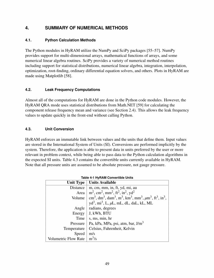
4. SUMMARY OF NUMERICAL METHODS

4.1. Python Calculation Methods

The Python modules in HyRAM utilize the NumPy and SciPy packages [55–57]. NumPyprovides support for multi-dimensional arrays, mathematical functions of arrays, and somenumerical linear algebra routines. SciPy provides a variety of numerical method routinesincluding support for statistical distributions, numerical linear algebra, integration, interpolation,optimization, root-finding, ordinary differential equation solvers, and others. Plots in HyRAM aremade using Matplotlib [58].

4.2. Leak Frequency Computations

Almost all of the computations for HyRAM are done in the Python code modules. However, theHyRAM QRA mode uses statistical distributions from Math.NET [59] for calculating thecomponent release frequency mean and variance (see Section 2.4). This allows the leak frequencyvalues to update quickly in the front-end without calling Python.

4.3. Unit Conversion

HyRAM enforces an immutable link between values and the units that define them. Input valuesare stored in the International System of Units (SI). Conversions are performed implicitly by thesystem. Therefore, the application is able to present data in units preferred by the user or morerelevant in problem context, while being able to pass data to the Python calculation algorithms inthe expected SI units. Table 4.3 contains the convertible units currently available in HyRAM.Note that all pressure units are assumed to be absolute pressure, not gauge pressure.

Table 4-1 HyRAM Convertible Units

Unit Type Units AvailableDistance m, cm, mm, in, ft, yd, mi, au

Area m2, cm2, mm2, ft2, in2, yd2

Volume cm3, dm3, dam3, m3, km3, mm3, µm3, ft3, in3,yd3, mi3, L, µL, mL, dL, daL, kL, ML

Angle radians, degreesEnergy J, kWh, BTU

Time s, ms, min, hrPressure Pa, kPa, MPa, psi, atm, bar, J/m3

Temperature Celsius, Fahrenheit, KelvinSpeed m/s

Volumetric Flow Rate m3/s

49

This page intentionally left blank.

50

5. ENGINEERING TOOLKIT

This section describes the Engineering Toolkit, which uses the models described elsewhere in thisreport to perform simple calculations for hydrogen properties.

5.1. Temperature, Pressure, and Density

The user can calculate one of the quantities temperature (T ), pressure (P), or density (ρ) byspecifying the other two. The algorithm uses the the CoolProp library [1] to perform thethermodynamic calculations (see Section 3.1.1).

5.2. Tank Mass

The user can calculate the mass (m) of hydrogen in a container by specifying the temperature (T ),pressure (P), and volume (V ) of the container.

m = ρV (120)

Where the density (ρ) is calculated using the CoolProp library [1] as described in Section 5.1.

5.3. Mass Flow Rate

The mass flow rate (m) of a leak from a tank can be calculated for either a steady release or for apressure blowdown of a tank. A "blowdown" describes the release of gas from a tank until thepressure reaches ambient, causing the mass flow to stop. This can be estimated from thetemperature (T ), pressure (P), and leak size ("Orifice Diameter", d) for a steady release, and alsovolume (V ) for a blowdown case.

For a steady-state release, the mass flow rate (m) is calculated using the density of the fluid (ρ),the velocity of the fluid through the orifice (v), and the area of the orifice (A)10:

m = ρvA (121)

The area of the orifice is given by the diameter of the orifice (d):

A =π

4d2 (122)

The density and velocity of the fluid depend on the temperature (T ) and pressure (P) of the tankand are calculated for the flowing fluid as described in Section 3.2.1. The output for the steadystate case is the mass flow rate in kg/s.10The discharge coefficient for the Engineering Toolkit is assumed to be equal to 1.0

51

For the blowdown case, the initial mass in the tank (m0) is calculated (same as Section 5.2) by:

m0 = ρ0V (123)

where ρ0 is the itinal density of hydrogen in the tank (which depends on the initial temperature(T ) and pressure (P) of the tank and is calculated as described in Section 5.1) and V is the volumeof the tank.

The mass and energy flow equations (as described in Section 3.3.2) are then integrated until thethe tank pressure is equal to ambient pressure (101,325 Pa). The output for the blowdown case isa combination plot of the mass in the tank, tank pressure, mass flow rate, and temperature overtime, as well as the total time needed for the tank to empty.

5.4. TNT Mass Equivalence

The TNT mass equivalence (mTNT equivalent) can be calculated using the flammable vapor releasemass (mfuel), the explosive energy yield (Y , 0–100%), and the net heat of combustion (∆Hc). Thisis calculated as:

mTNT equivalent =mfuel×Y ×∆Hc

4500 kJ/kgTNT(124)

The default heat of combustion is for hydrogen: ∆Hc, hydrogen = 120,000 kJ/kg [35, 36]. The TNTmass equivalence equation is taken from NUREG-1805 [60].

52

REFERENCES

[1] I. H. Bell, J. Wronski, S. Quoilin, and V. Lemort, “Pure and Pseudo-pure FluidThermophysical Property Evaluation and the Open-Source Thermophysical PropertyLibrary CoolProp,” Industrial & Engineering Chemistry Research, vol. 53, no. 6, pp.2498–2508, February 2014.

[2] J. W. Leachman, R. T. Jacobsen, S. G. Penoncello, and E. W. Lemmon, “Fundamentalequations of state for parahydrogen, normal hydrogen, and orthohydrogen,” Journal ofPhysical and Chemical Reference Data, vol. 38, no. 3, pp. 721–748, September 2009.

[3] J. M. Ohi, C. Moen, J. Keller, and R. Cox, “Risk assessment for hydrogen codes andstandards,” in Proceedings of the first International Conference on Hydrogen Safety, (ICHS2005), September 2005, pp. 8–10.

[4] J. LaChance, W. Houf, B. Middleton, and L. Fluer, “Analyses to support development ofrisk-informed separation distances for hydrogen codes and standards,” Sandia NationalLaboratories, SAND2009-0874, March 2009.

[5] J. LaChance, “Risk-informed separation distances for hydrogen refueling stations,”International Journal of Hydrogen Energy, vol. 34, no. 14, pp. 5838–5845, July 2009.

[6] J. LaChance, A. Tchouvelev, and J. Ohi, “Risk-informed process and tools for permittinghydrogen fueling stations,” International Journal of Hydrogen Energy, vol. 34, no. 14, pp.5855–5861, July 2009.

[7] J. L. LaChance, B. Middleton, and K. M. Groth, “Comparison of NFPA and ISO approachesfor evaluating separation distances,” International Journal of Hydrogen Energy, vol. 37,no. 22, pp. 17 488–17 496, November 2012.

[8] K. M. Groth, J. L. LaChance, and A. P. Harris, “Early-stage quantitative risk assessment tosupport development of codes and standard requirements for indoor fueling of hydrogenvehicles,” Sandia National Laboratories, SAND2012-10150, November 2012.

[9] ——, “Design-stage QRA for indoor vehicular hydrogen fueling systems,” in Proceedingsof the European Society for Reliability Annual Meeting (ESREL 2013), Amsterdam,September 29 - October 2 2013, pp. 2247–2256.

[10] A. V. Tchouvelev, K. M. Groth, P. Benard, and T. Jordan, “A hazard assessment toolkit forhydrogen applications,” in Proceedings of the 20th World Hydrogen Energy Conference(WHEC 2014), June 15 – 20 2014.

[11] H. J. Pasman, “Challenges to improve confidence level of risk assessment of hydrogentechnologies,” International Journal of Hydrogen Energy, vol. 36, no. 3, pp. 2407–2413,February 2011.

[12] K. Groth and A. Harris, “Hydrogen quantitative risk assessment workshop proceedings,”Sandia National Laboratories, SAND2013-7888, August 2013.

53

[13] K. Ham, A. Marangon, P. Middha, N. Versloot, N. Rosmuller, M. Carcassi, O. R. Hansen,M. Schiavetti, E. Papanikolaou, A. Venetsanos, A. Engebø, J. L. Saw, J.-B. Saffers,A. Flores, and D. Serbanescu, “Benchmark exercise on risk assessment methods applied to avirtual hydrogen refuelling station,” International Journal of Hydrogen Energy, vol. 36,no. 3, pp. 2666–2677, February 2011.

[14] A. Kotchourko, D. Baraldi, P. Benard, N. Eisenreich, T. Jordan, J. Keller, A. Kessler,J. LaChance, V. Molkov, M. Steen, A. Tchouvelev, and J. Wen, “State of the art and researchpriorities in hydrogen safety,” Joint Research Centre of the European Commission (JRC), ,March 2014.

[15] A. V. Tchouvelev, “Knowledge gaps in hydrogen safety: A white paper,” InternationalEnergy Agency Hydrogen Implementing Agreement Task 19, , January 2008.

[16] K. M. Groth and A. V. Tchouvelev, “A toolkit for integrated deterministic and probabilisticrisk assessment for hydrogen infrastructure,” in Proceedings of the International Conferenceon Probabilistic Safety Assessment and Management (PSAM 12), Honolulu, HI, June 22–272014.

[17] Center for Chemical Process Safety (CCPS), Guidelines for Chemical Process QuantitativeRisk Analysis. American Institute of Chemical Engineers, 1999.

[18] T. Aven, Foundations of risk analysis. John Wiley & Sons, 2003.

[19] M. Modarres, Risk Analysis in Engineering: Techniques, Tools, and Trends. CRC Press,2006.

[20] SFPE, “SFPE engineering guide to performance-based fire protection analysis and design ofbuildings,” National Fire Protection Association, Quincy, MA, USA, , 2007.

[21] S. E. Rose, S. Flamberg, and F. Leverenz, Guidance Document for Incorporating RiskConcepts into NFPA Codes and Standards. Fire Protection Research Foundation, March2007.

[22] J.-E. Vinnem, Offshore Risk Assessment: Principles, Modelling and Applications of QRAStudies, 2nd ed. Springer, 2007.

[23] T. Aven, Quantitative risk assessment: the scientific platform. Cambridge UniversityPress, 2011.

[24] B. D. Ehrhart, D. Brooks, A. B. Muna, and C. LaFleur, “Evaluation of risk acceptancecriteria for transporting hazardous materials,” DOT Federal Railway Administration,DOT/FRA/ORD-20/06, February 2020.

[25] B. D. Ehrhart, E. S. Hecht, and J. A. Mohmand, “Validation and comparison of HyRAMphysics models,” Sandia National Laboratories, SAND2021-5811, May 2021.

[26] W. Houf and R. Schefer, “Predicting radiative heat fluxes and flammability envelopes fromunintended releases of hydrogen,” International Journal of Hydrogen Energy, vol. 32, no. 1,pp. 136–151, January 2007.

54

[27] I. W. Ekoto, A. J. Ruggles, L. W. Creitz, and J. X. Li, “Updated jet flame radiation modelingwith buoyancy corrections,” International Journal of Hydrogen Energy, vol. 39, no. 35, pp.20 570–20 577, December 2014.

[28] J. LaChance, A. Tchouvelev, and A. Engebø, “Development of uniform harm criteria for usein quantitative risk analysis of the hydrogen infrastructure,” International Journal ofHydrogen Energy, vol. 36, no. 3, pp. 2381–2388, February 2011.

[29] N. A. Eisenberg, C. J. Lynch, and R. J. Breeding, “Vulnerability model. A simulation systemfor assessing damage resulting from marine spills,” U.S. Coast Guard, SA/A-015 245, 1975.

[30] C. K. Tsao and W. W. Perry, “Modifications to the vulnerability model: a simulation systemfor assessing damage resulting from marine spills,” U.S. Coast Guard, ADA 075 231, 1979.

[31] TNO, “Methods for the determination of possible damage,” The Netherlands Organizationof Applied Scientific Research (TNO), CPR 16E, 1992.

[32] F. P. Lees, “The assessment of major hazards: a model for fatal injury from burns,” ProcessSafety and Environmental Protection, vol. 72, no. 3, pp. 127–134, 1994.

[33] HSE, Major hazard aspects of the transport of dangerous substances. UK Health andSafety Executive, 1991.

[34] ——, “Methods of approximation and determination of human vulnerability for offshoremajor accident hazard assessment,” UK Health and Safety Executive, , 2010.

[35] F. P. Lees, Lees’ Loss Prevention in the Process Industries, 3rd ed., S. Mannan, Ed.Elsevier Science & Technology, 2005.

[36] M. J. Hurley, D. T. Gottuk, J. R. H. Jr., K. Harada, E. D. Kuligowski, M. Puchovsky, J. L.Torero, J. M. W. Jr., and C. J. Wieczorek, Eds., SFPE Handbook of Fire ProtectionEngineering, 5th ed. Springer, New York, NY, 2016.

[37] M.-S. Chung, S.-B. Park, and H.-K. Lee, “Sound speed criterion for two-phase critical flow,”Journal of Sound and Vibration, vol. 276, no. 1, pp. 13–26, 2004.

[38] B. D. Ehrhart and E. S. Hecht, “Hydrogen risk assessment models (HyRAM) version 3.0technical reference manual,” Sandia National Laboratories, SAND2020-10600, September2020.

[39] K. B. Yüceil and M. V. Ötügen, “Scaling parameters for underexpanded supersonic jets,”Physics of Fluids, vol. 14, no. 12, pp. 4206–4215, October 2002.

[40] A. D. Birch, D. J. Hughes, and F. Swaffield, “Velocity decay of high pressure jets,”Combustion Science and Technology, vol. 52, no. 1-3, pp. 161–171, 1987.

[41] A. D. Birch, D. R. Brown, M. G. Dodson, and F. Swaffield, “The structure and concentrationdecay of high pressure jets of natural gas,” Combustion Science and Technology, vol. 36, no.5-6, pp. 249–261, 1984.

[42] B. C. R. Ewan and K. Moodie, “Structure and velocity measurements in underexpandedjets,” Combustion Science and Technology, vol. 45, no. 5-6, pp. 275–288, 1986.

55

[43] V. Molkov, D. Makarov, and M. Bragin, “Physics and modelling of under-expanded jets andhydrogen dispersion in atmosphere,” in Proceedings of the 24th international conference oninteraction of intense energy fluxes with matter, March 1-6 2009.

[44] W. Houf and W. Winters, “Simulation of high-pressure liquid hydrogen releases,”International Journal of Hydrogen Energy, vol. 38, no. 19, pp. 8092–8099, June 2013.

[45] W. S. Winters, “Modeling leaks from liquid hydrogen storage systems,” Sandia NationalLaboratories, SAND2009-0035, January 2009.

[46] G. Abraham, “Horizontal jets in stagnant fluid of other density,” Journal of the HydraulicsDivision, vol. 91, no. 4, pp. 139–154, 1965.

[47] W. Houf and R. Schefer, “Analytical and experimental investigation of small-scaleunintended releases of hydrogen,” International Journal of Hydrogen Energy, vol. 33, no. 4,pp. 1435–1444, February 2008.

[48] M. Hosseini, I. Dincer, G. Naterer, and M. Rosen, “Thermodynamic analysis of fillingcompressed gaseous hydrogen storage tanks,” International Journal of Hydrogen Energy,vol. 37, no. 6, pp. 5063–5071, March 2012.

[49] B. Lowesmith, G. Hankinson, C. Spataru, and M. Stobbart, “Gas build-up in a domesticproperty following releases of methane/hydrogen mixtures,” International Journal ofHydrogen Energy, vol. 34, no. 14, pp. 5932–5939, July 2009.

[50] P. P. Panda and E. S. Hecht, “Ignition and flame characteristics of cryogenic hydrogenreleases,” International Journal of Hydrogen Energy, vol. 42, no. 1, pp. 775–785, January2017.

[51] A. Molina, R. W. Schefer, and W. G. Houf, “Radiative fraction and optical thickness inlarge-scale hydrogen-jet fires,” Proceedings of the Combustion Institute, vol. 31, no. 2, pp.2565–2572, January 2007.

[52] F. D. Wayne, “An economical formula for calculating atmospheric infrared transmissivities,”Journal of Loss Prevention in the Process Industries, vol. 4, no. 2, pp. 86 – 92, January 1991.

[53] G. Hankinson and B. J. Lowesmith, “A consideration of methods of determining theradiative characteristics of jet fires,” Combustion and Flame, vol. 159, no. 3, pp. 1165–1177,March 2012.

[54] C. Bauwens and S. Dorofeev, “CFD modeling and consequence analysis of an accidentalhydrogen release in a large scale facility,” International Journal of Hydrogen Energy,vol. 39, no. 35, pp. 20 447–20 454, December 2014.

[55] T. E. Oliphant, A guide to NumPy. Trelgol Publishing USA, 2006, vol. 1.

[56] S. Van Der Walt, S. C. Colbert, and G. Varoquaux, “The numpy array: a structure forefficient numerical computation,” Computing in Science & Engineering, vol. 13, no. 2,p. 22, 2011.

56

[57] P. Virtanen, R. Gommers, T. E. Oliphant, M. Haberland, T. Reddy, D. Cournapeau,E. Burovski, P. Peterson, W. Weckesser, J. Bright, S. J. van der Walt, M. Brett, J. Wilson,K. Jarrod Millman, N. Mayorov, A. R. J. Nelson, E. Jones, R. Kern, E. Larson, C. Carey,I. Polat, Y. Feng, E. W. Moore, J. VanderPlas, D. Laxalde, J. Perktold, R. Cimrman,I. Henriksen, E. A. Quintero, C. R. Harris, A. M. Archibald, A. H. Ribeiro, F. Pedregosa,P. van Mulbregt, and SciPy 1.0 Contributors, “SciPy 1.0: Fundamental Algorithms forScientific Computing in Python,” Nature Methods, vol. 17, pp. 261–272, 2020.

[58] J. D. Hunter, “Matplotlib: A 2D graphics environment,” Computing in Science &Engineering, vol. 9, no. 3, pp. 90–95, 2007.

[59] Math.net numerics. [Online]. Available: http://numerics.matdotnet.com

[60] N. Iqbal and M. H. Salley, “Fire Dynamics Tools (FDTs): Quantitative Fire Hazard AnalysisMethods for the U.S. Nuclear Regulatory Commission Fire Protection Inspection Program,”U.S. Nuclear Regulatory Commission, Washington, DC, NUREG-1805, December 2004.

57

DISTRIBUTION

Email—External (encrypt for OUO)

NameCompany Email

AddressCompany Name

Laura Hill laura.hill@ee.doe.gov DOE HFTO

Email—Internal (encrypt for OUO)

Name Org. Sandia Email Address

Ethan Hecht 08367 ehecht@sandia.gov

Joseph Ronevich 08367 jaronev@sandia.gov

Chris San Marchi 08367 cwsanma@sandia.gov

Brian Ehrhart 08854 bdehrha@sandia.gov

Chris LaFleur 08854 aclafle@sandia.gov

Scott Sanborn 08854 sesanbo@sandia.gov

Technical Library 1911 sanddocs@sandia.gov

58

Sandia National Laboratories is amultimission laboratory managedand operated by NationalTechnology & EngineeringSolutions of Sandia LLC, a whollyowned subsidiary of HoneywellInternational Inc., for the U.S.Department of Energy’s NationalNuclear Security Administrationunder contract DE-NA0003525.