Hydrological assessment to predict velocity-flow classes

Hydrological assessment to predict velocity-flow classes in the lower Thukela

River

PG Jacobs

22707506

Dissertation submitted in fulfilment of the requirements for the degree Magister Scientiae in Environmental Science (specialising in Hydrology and Geohydrology) at the Potchefstroom Campus of the North-West University

Supervisor: Dr SR Dennis

Co-Supervisor: Dr G O’Brien

May 2017

i

ACKNOWLEDGEMENTS

“With man this is impossible, but with God all things are possible.”

~ Matthew 19:26

I would like to thank the following people for their contribution and help throughout the

project:

My supervisor Dr SR Dennis for the insight, support and guidance throughout the two

years as well as for the equipment made available for field trips, it is really

appreciated.

My co-supervisor Dr Gordon O’Brien thank you for the opportunities you have

provided over the past 5 years to work on numerous projects and for the funding

made available for this study, I am truly thankful and my Masters would not have

been possible without you.

My brother and mentor Francois Jacobs for spending many hours helping me with

fieldwork, preparations and motivation. For spending a lot of time helping me with

structure and data analysis. Thank you

I must also express my profound gratitude to my parents Naas and Kobie Jacobs for

their continuous support and encouragement throughout my years of study.

I would also like to thank my fiancé Marlene Kruger for believing in me and her

consistent support over the past years, I will be forever grateful for her love.

In addition I would like to thank the following people for helping me with data collection, field

work, insight and the organisation of surveys without their help the study would not have

been possible:

Wesley Evans – Specifically for fish data

Mahomed Desai

Lungelo Madiya

Ntaki Senogo

Gerhard Jacobs

ii

ABSTRACT

This study investigates the use of a two-dimensional hydrodynamic model (River2D) to

determine environmental flow requirements in the lower Thukela River, KwaZulu-Natal. A

digital elevation model (DEM) was developed by combining bathymetric data from field

surveys with topographic data in ArcGIS. HECGeo-RAS was used to delineate cross-

sections, flow boundaries, river banks and flood plains from the DEM. Data were imported to

HEC-RAS were a series of flows were simulated to generate a stage-discharge curve. The

predicted stage generated by HEC-RAS was used to set the downstream boundary

conditions in River2D. The 2-dimensional modelling techniques used in this study make use

of a combination of three different programs namely: BED, MESH and River2D to create a

river bed profile that can be used for complex calculations.

To determine the habitat requirements and preferences, 19 freshwater and estuarine fish

species relevant to the lower Thukela River were used in the analyses. Multivariate statistical

analysis showed that some species community structures changed significantly with a

change in substrate and velocity. Labeobarbus natalensis and Eleotris fusca were the

identified indicator species for this study. Preference files were generated for each species

as well as habitat suitability according to field data. To determine the environmental flow

requirements (EFR) of the lower Thukela River, historic and habitat methods were used and

compared. River2D make use of the PHABSIM concept to calculate weighted usable area

(WUA) (m2/m) by combining habitat suitability with velocity and depth preferences. The EFR

suggested by the historic methods for the lower Thukela River is too low and does not

consider the anthropogenic changes upstream of the study site and therefore the habitat

method in the form of WUA was recommended.

Keywords: Velocity-flow classes; River2D; biological indicator; preference files; weighted

usable area; environmental flow requirements

iii

SAMEVATTING

Hierdie studie ondersoek die gebruik van 'n twee-dimensionele hidrodinamiese model

(River2D) om omgewingsvloeivereistes te bepaal in die laer Thukela-rivier, KwaZulu-Natal. ŉ

Digitale elevasie model (DEM) is ontwikkel in ArcGIS deur die kombinasie van velddata en

topografiese data. HECGeo-RAS is gebruik om deursnitdata, rivier-oewers, en vloedvlaktes

te genereer vanaf die DEM en is dan in HEC-RAS ingevoer. Addisionele vloei is gesimuleer

om waterelevasievlakke te skep wat as grenstoestande in River2D gebruik is. Die 2-

dimensionele model wat in hierdie studie gebruik is, maak van 'n kombinasie van drie

verskillende programme gebruik, naamlik: BED, MESH en River2D om ŉ rivier bodemprofiel

te skep wat gebruik kan word vir komplekse berekeninge.

19 varswater- en riviermondings visspesies relevant tot die laer Thukela-rivier is gebruik om

habitatvereistes en voorkeure te bepaal. Statistiese analise het getoon dat

gemeenskapstrukture van sommige spesies aansienlik verander as gevolg van ŉ

verandering van substraat of vloeisnelheid. Labeobarbus natalensis en Eleotris fusca is as

ekologiese aanwyserspesies vir hierdie studie geïdentifiseer. Habitatvereistes en

voorkeurlêers vir snelheid, diepte en substraat is gegenereer vir elke spesie. Historiese- en

habitatmetodes is gebruik en vergelyk om omgewingsvloeivereistes te bepaal vir die laer

Thukela-rivier. River2D maak gebruik van die PHABSIM konsep om geweegde bruikbare

area (m2/m) te bereken deur habitatsgeskiktheid met vloei snelheid en diepte te kombineer.

Die omgewingsvloeivereistes voorgestel deur die historiesemetodes is te laag en neem nie

menslike verandering stroomop in ag nie en daarom word die habitatmetode voorgestel.

Sleutelwoorde: Habitat-klasse; River2D; ekologiese-aanwyser; voorkeurlêers; geweegde

bruikbare area; omgewingsvloeivereistes

iv

Table of Contents

ACKNOWLEDGEMENTS ...................................................................................................... i

ABSTRACT ...........................................................................................................................ii

SAMEVATTING .................................................................................................................... iii

LIST OF FIGURES ............................................................................................................... vi

LIST OF TABLES ................................................................................................................. x

ABBREVIATIONS ................................................................................................................ xi

1. General introduction ....................................................................................................... 1

1.1. Problem Statement ................................................................................................. 2

1.2. Hypotheses ............................................................................................................. 3

1.3. Aims and objectives ................................................................................................ 3

1.4. Dissertation structure .............................................................................................. 4

2. Literature Review ........................................................................................................... 6

2.1. Bioregions and ecoregions ...................................................................................... 6

2.2. River Landscapes ................................................................................................... 7

2.3. Eco-hydraulics ...................................................................................................... 14

2.4. Flows and channel morphology............................................................................. 16

2.5. River channels ...................................................................................................... 16

2.6. Eco-hydraulic modelling ........................................................................................ 21

2.7. Fish as indicator species ....................................................................................... 24

2.8. Significant elements of the flow regime ................................................................. 25

2.9. Ecological flow assesment methods ..................................................................... 26

3. Materials and methods ................................................................................................. 29

3.1. Study area ............................................................................................................ 29

3.2. Climate ................................................................................................................. 32

3.3. Geology ................................................................................................................ 33

3.4. Hydrological Data collection .................................................................................. 37

3.5. Fish collection ....................................................................................................... 40

3.6. Data analyses ....................................................................................................... 43

v

3.6.1. Field Measurements ...................................................................................... 43

3.6.2. DEM and cross sections generated ............................................................... 44

3.6.3. Model selection .............................................................................................. 44

3.6.4. HEC-RAS analyses........................................................................................ 45

3.6.5. River2D data analyses ................................................................................... 45

3.7. Ecological wellbeing of fish in the Thukela River ................................................... 48

3.7.1. Response of communities to habitat variable condition alterations ................. 49

3.7.2. Habitat preference assessment ..................................................................... 50

3.8. Historic method for calculating ecological flow requirements ................................. 51

3.9. Instream flow incremental methodology ................................................................ 52

4. Results and Discussion ................................................................................................ 53

4.1. DEM creation, predicting water levels and velocity-flow classes ........................... 53

4.2. River 2D ................................................................................................................ 57

4.3. Fish collection and preferences............................................................................. 70

4.3.1. Response of fish community structures to habitat variable conditions ............ 72

4.3.2. Habitat preference assessment ..................................................................... 75

4.3.3. The effects that altered flows will have on the lower Thukela River ................ 79

4.4. Ecological flow requirements ................................................................................ 80

5. Conclusion ................................................................................................................... 92

6. Recommendations ....................................................................................................... 95

7. References .................................................................................................................. 96

Appendix A ............................................................................................................................ I

Appendix B .......................................................................................................................... IX

vi

LIST OF FIGURES

Figure 1: Population density and distribution in South Africa (Statistics, 2013) ...................... 2

Figure 2: Ecoregion distribution of South Africa (Kleynhans et al., 2005) .............................. 8

Figure 3: The South African hierarchical system (Rowntree & Wadeson, 1999) .................. 11

Figure 4: Gaining and losing river systems. Water is either transported from the shallow

aquifer into the river system (gaining stream) or water is lost from the river into the shallow

aquifer (losing stream) (Stute, 2002). .................................................................................. 12

Figure 5: Model of an ecohydrological system (James, 2008) ............................................. 15

Figure 6: The four velocity-depth flow classes used in this study(Kleynhans, 1999). ........... 20

Figure 7: Empirical vs. deterministic modelling of hydraulic conditions ................................ 23

Figure 8: The study area on the lower Thukela River. ......................................................... 31

Figure 9: Secondary and tertiary catchments of the Thukela system. .................................. 32

Figure 10: Simplified geological map of the Thukela River catchment ................................. 36

Figure 11: Data coverage on the lower Thukela River during this study. ............................. 38

Figure 12: A) One of the benchmarks installed in April 2015 on the first survey for a cross-

section to get a stage discharge profile, B) Setting up the Total station to complete the cross

section. C) One of the crocodile encounters at a cross-section profile, D) Showing a single

channel for one of the cross-sections, E) Ntaki measuring flow velocities with the flow meter,

F) Starting a cross-section close and working the way back, G) Testing the prism to make

sure it works before starting the cross-sections. .................................................................. 39

Figure 13: Sampiling methods used for fish collection during surveys included: A) Seine

nets, B) Casting net, C) Electrofishing and D) Scoop net .................................................... 41

Figure 14: The different habitats used for the channel index substrate in the WUA

calculations. A) Silt, B) Sand, C and D) Gravel, E) Sand cover area, F) Bedrock, G)

Vegetated overbanks .......................................................................................................... 42

Figure 15: Velocity-area method based on the velocity at 60% of the depth (John, 2001). .. 43

vii

Figure 16: Comparisons/overlaps in scoring systems of the Lines of Evidence used in the

study to represent fish health (FRAI), community structures and community wellbeing. ...... 49

Figure 17: Topographic data used to generate a DEM. ....................................................... 53

Figure 18: Additional bathymetric data created with HEC-GeoRAS before exporting it into

HEC-RAS. ........................................................................................................................... 54

Figure 19: The comparison between HEC-RAS simulated water levels and measured water

levels along the thalweg after calibration with a discharge of 4.3 m3/s. ................................ 55

Figure 20: Correlation between measured and simulated water levels at different cross-

sections using HEC-RAS after model calibration. ................................................................ 55

Figure 21: Stage vs. Discharge simulated from HEC-RAS model for the lower boundary

conditions in River2D. ......................................................................................................... 57

Figure 22: The comparison between River2D simulated water levels and measured water

levels along the thalweg after calibration with a discharge of 4.3 m3/s. ................................ 58

Figure 23: Correlation between measured and simulated water levels at cross-sections using

River2D after model calibration. .......................................................................................... 59

Figure 24: Site 1: cross-section, the inflow boundary for River2D A) Total station setup, B)

View across river, C) View upstream, D) View downstream. ............................................... 60

Figure 25: Simulated vs. Measured velocities for cross section 1 over bed topography and

depth. .................................................................................................................................. 61

Figure 26: Site 2 A) Total station setup, B) View across river, C) View upstream, D) View

downstream ........................................................................................................................ 62

Figure 27: Simulated vs. Measured velocity for cross section 2 over bed topography and

depth. .................................................................................................................................. 63

Figure 28: Site 3 with steep bedrock on the opposite bank A) Total station setup, B) View

across river, C) View upstream, D) View downstream ......................................................... 64


depth. .................................................................................................................................. 65

viii


downstream ........................................................................................................................ 66


depth. .................................................................................................................................. 67

Figure 32: Cross-section 5 (Sand mining two) with cobbles and silt as substrate A) Total

station setup, B) View across river, C) View upstream, D) View downstream ...................... 68


depth. .................................................................................................................................. 69

Figure 34: Fish species sampled during surveys in the Lower Thukela River included A)

Glossogobius callidus, B) Eleotris fusca, C) Enteromius eutaenia, D) Enteromius

trimaculatus, E) Labeobarbus natalensis (juvenile), F) Labeobarbus natalensis (adult), G)

Pseudocrenilabrus philander, H) Labeo molybdinus, I) Oreochromis mossambicus, J)

Acanthopagrus berda, K) Anguilla marmorata, L) Clarias gariepinus and M) Myxus capensis

........................................................................................................................................... 71

Figure 35: Redundancy analyses plot showing correlation between fish species and

substrate types. With a variance in fish community structures for axis 1 = 60.7% and

additional 26.5% and on axis 2 = 87.2% of variability displayed on graph. .......................... 73

Figure 36: Redundancy analyses plot showing correlation between fish species and velocity-

depth classes. With a variance in fish community structures for axis 1 = 84.5% and

additional 15.5% and on axis 2 = 100% of variability displayed on graph. ........................... 74

Figure 37: Box (25th to 75th percentile) and whisker (max and min value) for water velocity

habitats associated with species observations in KZN. ....................................................... 75

Figure 38: Box (25th to 75th %tile) and whisker (max and min value) for water depth habitats

associated with species observations. ................................................................................ 76

Figure 39: Velocity (m/s) and depth (mm) preference relationship for Labeobarbus natalensis

with abundances displayed as bubbles. .............................................................................. 77

Figure 40: Velocity (m/s) and depth (mm) preference relationship for Eleotris fusca with

abundances displayed as bubbles. ..................................................................................... 78

Figure 41: Fish preferences in relationship with substrate types ......................................... 79

ix

Figure 42: Flow duration curve for the median flow and the base flow for the lower Thukela

River based on historic data ................................................................................................ 81

Figure 43: Flows for different months using the Tennants (1976) method to predict critical

base, base, median and freshes flows for the lower Thukela River ..................................... 82

Figure 44: Aquatic Base Flow method vs. Tennant (1976) method for base flows ............... 83

Figure 45: Selection of minimum flow for L. natalensis at the breakpoint: point where habitat

begins to degrade sharply with a decrease in flow .............................................................. 85

Figure 46: Selection of minimum flow for E. fusca at the breakpoint: point where habitat

begins to degrade sharply with a decrease in flow .............................................................. 85

Figure 47: WUA for L. natalensis at their minimum flow requirement of 15 m3/s for the 4.6 km

study area in the lower Thukela River as predicted by the IFIM methodology. .................... 90

Figure 48: WUA for E. fusca at their minimum flow requirement of 8 m3/s for the 4.6 km

study area in the lower Thukela River as predicted by the IFIM methodology. .................... 91

x

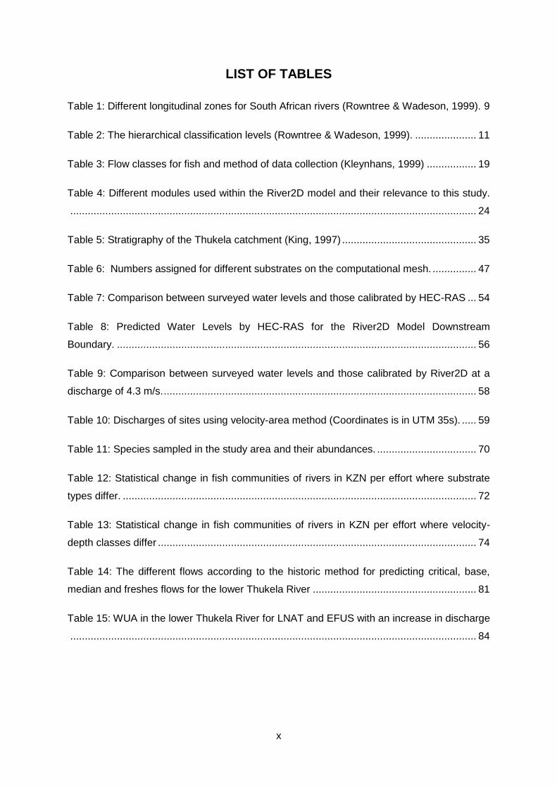
LIST OF TABLES

Table 1: Different longitudinal zones for South African rivers (Rowntree & Wadeson, 1999). 9

Table 2: The hierarchical classification levels (Rowntree & Wadeson, 1999). ..................... 11

Table 3: Flow classes for fish and method of data collection (Kleynhans, 1999) ................. 19

Table 4: Different modules used within the River2D model and their relevance to this study.

........................................................................................................................................... 24

Table 5: Stratigraphy of the Thukela catchment (King, 1997) .............................................. 35

Table 6: Numbers assigned for different substrates on the computational mesh. ............... 47

Table 7: Comparison between surveyed water levels and those calibrated by HEC-RAS ... 54

Table 8: Predicted Water Levels by HEC-RAS for the River2D Model Downstream

Boundary. ........................................................................................................................... 56

Table 9: Comparison between surveyed water levels and those calibrated by River2D at a

discharge of 4.3 m/s. ........................................................................................................... 58

Table 10: Discharges of sites using velocity-area method (Coordinates is in UTM 35s). ..... 59

Table 11: Species sampled in the study area and their abundances. .................................. 70

Table 12: Statistical change in fish communities of rivers in KZN per effort where substrate

types differ. ......................................................................................................................... 72

Table 13: Statistical change in fish communities of rivers in KZN per effort where velocity-

depth classes differ ............................................................................................................. 74

Table 14: The different flows according to the historic method for predicting critical, base,

median and freshes flows for the lower Thukela River ........................................................ 81

Table 15: WUA in the lower Thukela River for LNAT and EFUS with an increase in discharge

........................................................................................................................................... 84

xi

ABBREVIATIONS

1D One Dimensional

2D Two Dimensional

ABF Aquatic Base Flow

ADCP Acoustic Doppler Current Profiler

ATTZ Aquatic Terrestrial Transition Zone

BBM Building Block Method

CSI Composite Suitability Index

CSI Combined Suitability Index

DEM Digital Elevation Model

DTM Digital Terrain Model

DWS Department of Water and Sanitation

EFR Ecological Flow Requirements

FIFHA Fish Invertebrate Flow Habitat Assessment

FRAI Fish Response Assessment Index

GIS Geographic Information System

GUI Graphical User Interface

HSC Habitat Suitability Criteria

IFIM Instream Flow Incremental Methodology

IFR Instream Flow Requirements

LHDA Lesotho Highlands Development Authority

LHWP Lesotho Highlands Water Project

LoEs Lines of Evidence

MAE Mean Annual Evaporation

MALF Mean Annual Low Flow

MAP Mean Annual Precipitation

MAR Mean Annual Runoff

QI Quality Index

RCC River Continuum Concept

RDA Redundancy Analyses

RES Riverine Ecosystem Synthesis

SI Suitability Index

TIN Triangulated Irregular Network

TVHR Transparent Velocity Head Rod

UTM Universal Transverse Mercator

WUA Weighted Useable Area

1

1. General introduction

Worldwide more than 2.3 billion people live in already water stressed areas where they have

an annual per capita water availability of below the world average of 1 700 m3 (WRI, 2008).

South Africa currently has a population of about 53 million people which ranks it at number

24 out of the 25 most populated countries in the world (Statistics, 2013). The uneven

distribution of the South African population makes water management challenging as the

country mostly consists of an arid to semi-arid landscape and therefore most of the

population densities (Figure 1) are concentrated on smaller areas resulting in an increase in

environmental impacts.

The current water availability of 1 100 m3 per capita of South Africans is under serious stress

(Johansson, 1993). According to the DWA (2011) “Less than 10% of South Africa’s rainfall is

available as surface water, one of the lowest conversion ratios in the world.” By further

altering the natural flow system of a river through the construction of dams, weirs and

bridges, ecosystems are more threatened today. With an increase in technology, excessive

groundwater extraction is further contributing to the deterioration of the natural water

resources (Postel, 2000). South Africa’s main rivers face great dangers as only 30% are still

preserved and sustainable, while 47% are modified for human benefits and 23% have been

transformed to a state where they are irreversible (Nel et al., 2007).

It is impossible for humankind to live in urban agglomerations, producing food and consumer

goods, expanding their technological development, without increasing the production of

wastes, and especially without having a large part of these wastes reaching the water bodies

(Perry & Vanderklein, 2009). Water management is probably the biggest environmental

challenge and over the next 30 years the predicted water demand will increase with 52%

(Walmsley et al., 1999).

The available fresh surface water on earth only makes up a minuscule portion of 0.01% of

the world’s water, yet it contains more than a 100 000 species out of the 1.8 million species

described on earth (Dudgeon et al., 2006). Freshwater is considered the most vital resource

on earth and its conservation was declared as a priority during the international Decade for

Action “Water for Life” 2005-2015 (Dudgeon et al., 2006). The conservation and

management of these ecosystems are critical as they provide a valuable natural resource to

cultural, scientific, aesthetic and economical progression which is of interest to all humans,

nations and governments (Dudgeon et al., 2006). Ecosystems are in great danger because

of population growth which results in overexploitation, habitat degradation, water pollution

2

and flow modifications, therefore the conservation of freshwater ecosystems is one of the

biggest environmental challenges that our generation faces (Dudgeon et al., 2006).

Figure 1: Population density and distribution in South Africa (Statistics, 2013).

1.1. Problem Statement

The Lower Thukela Bulk Water Infrastructure Project in Mandini includes the construction of

a new dam on the Thukela River. This will reduce water demand from the Hazelmere Dam

which currently provides water for the iLembe District. Construction of the bulk water supply

scheme will provide sufficient water for the KwaDukuza and the Mandini local Municipalities

in the eThekwini district. The purpose of the project is to supply 55 Ml/d of treated water in

phase one and ultimately a total of 110 Ml/d. The new dam in the Lower Thukela River could

possibly have a major impact on the flow regime downstream. Ecological flow requirements

for the lower Thukela River are not only important on a socio-economic level but also for the

ecological state of the river. It is important to protect the aquatic habitat and therefore sustain

flows as close to natural flows as possible. Different fish species have different flow

3

requirements to migrate upstream, spawn and feed at different times of the year and for

different periods. The regulation of flow will have a direct impact on the natural flow regime

and therefore it is important to predict these requirements. The bulk water supply scheme is

not the only anthropogenic buffer in the lower Thukela River but Sappi abstract water for

industrial use from an artificial barrier established for the mill (Hocking, 1987). Disturbing the

natural flow regime will have a negative effect on the aquatic ecology within a river and

therefore it is important to understand and evaluate the extend of these impacts on the

natural diversity in the ecological ecosystem. Flow alteration affects river hydrology and to

link these changes to ecosystem processes eco-hydraulics were used, which links

hydrological processes to instream habitat conditions. By modelling the hydraulics of a river

it is possible to understand the instream hydraulic habitat that forms the basis of the aquatic

ecosystem. As discharge increase so does flow velocity and depth, but this relationship is

complex and related to the shape of the river channel as well as the “roughness” of the

river’s substrate. Different parts of the river become inundated at different water levels and

detailed on-site measurements and numerical modelling are required to determine the

hydraulics of a river system.

1.2. Hypotheses

The hypotheses established for this study state:

1. The change in hydrological flow can be linked to habitat using a combination of GIS,

HEC-GeoRAS and HEC-RAS.

2. Habitat preferences of fish can be used with hydraulic models to evaluate the

environmental flow requirements and consequences of altered flows in the lower

Thukela River.

1.3. Aims and objectives

The aims established for this study include the following:

1. Conduct an open water hydrological assessment to predict the different habitat

classes for indicator fish species. In order to achieve this aim the following objectives

have been established:

a. Collect bathymetric data of an appropriate reach of the lower Thukela River

and create a 2-Dimensional model to predict habitat flow classes.

4

b. Collect topographic data for the study area at an acceptable accuracy for the

2D model.

2. Evaluate the flow dependant habitat requirements for indicator fish species in the

lower Thukela River and how flow alterations will affect fish preferences for different

cover types.

a. Identify some indicator fish species with a good variability in preferences for

different habitats associated with flows.

b. Create preference relationships for each indicator species.

3. Predict the EFR and determine a baseline flow for the Thukela River not only to

maintain the ecological state of the river but also to improve the current state by

using fish as ecological indicators.

a. Use different instream flow assessments to calculate the flow requirements

for indicator species by making use of historic methods and habitat methods.

1.4. Dissertation structure

Chapter 1: Introduction

Emphasise the importance of freshwater ecosystems, the problem statement as well

as the aims and objectives set out to complete this study.

Chapter 2: Literature Review

Discuss the scope of research done prior to field work and provide an outline of

physical and ecological aspects that form and take part in a river ecosystem.

Chapter 3: Materials and Methods

Description of the study area with climate and geology.

Description of the materials and methods used to complete the study as well as data

collection and manipulation techniques.

Chapter 4: Results and Discussion

Presents an overview of results obtained and a detailed discussion and interpretation

of the results obtained throughout the study and a comparison of the different

techniques for ecological flow requirements.

5

Chapter 5: Conclusion and Recommendations

Summary of the results obtained in the study and the conclusion drawn as well as

recommendations for future studies.

Chapter 6: References

A complete list of references cited in the chapters of this document.

6

2. Literature Review

2.1. Bioregions and ecoregions

The varying geology and geomorphology in South Africa is because of millions of years of

continental movement and erosion as well as the climatic range from semi-arid to arid

condition and have resulted in diverse ecosystems, including river ecosystems (Lamouroux

et al., 2002). Organisms living in rivers had to adapt over millions of years to cope with their

abiotic and biotic environments and therefore the communities of plants and animals tend to

be structured rather than random in any given river (Lamouroux et al., 2002). Bio-

geographical history of the region like climate, geology and topography will constrain the

suite of potential species to the regional species pool. Species with suitable morphological,

behavioural and life-history attributes will persist in any given river system (Lamouroux et al.,

2002).

Eekhout et al. (1997) used three groups of riverine organisms (riparian plants, invertebrates

and fish) at a tertiary catchment level delineating bio-geographical regions for South Africa.

This with detailed information on physiography was used to produce 18 bioregions for South

Africa (Brown et al., 1996).

Allanson et al. (2012) used geomorphological, geochemical and climatological features to

describe and define five limnological regions within Southern Africa. These regions describe

broad suites or typical assemblages of species that form the regional species pools.

More recently the South African landscape and variable geographic data was used to create

an ecoregion map for Swaziland, Lesotho and South Africa (Figure 2). The key variables

used in the typing were morphological classes and natural vegetation which is considered as

an integrated variable of climate, geology, rainfall and soil. Ecoregion classification has

become the basis for the grouping of rivers because it provides a broad indication of types of

rivers, and types of animal and plant communities, one could expect to find in any part of the

country. Information used to classify each of the 31 ecoregions is (Brown et al., 2007):

Main vegetation types

Terrain morphology

Mean annual precipitation

Coefficient of variation of mean annual precipitation

Drainage density

Stream frequency

7

Slope

Median annual simulated runoff

Mean annual temperature

2.2. River Landscapes

The change in the quantity and quality of water through its passage across the landscape

from headwater to sea, annual floods, and the sequences of fast and slow moving water all

contribute to the diversity of landscapes found in rivers (James & King, 2010). Water flowing

downstream has the ability to do work in the form of turbulence and sound. The interaction of

water and sediment during downward flow will shape the river bed and banks of the channel,

thus forming distinctive features in the river landscape such as cobble bars, sand bars,

islands, floodplains, meanders, deltas and beaches (James & King, 2010). Water flowing

through over and around these features will provide physical living space for organisms in

the form of habitat. According to Southwood (1988), it is important to understand the

physical nature of the riverscape to be able to predict what type of organisms will exist in that

river.

Two common features of rivers are:

They are heterogeneous which means that they provide a variety of different habitats

for organisms.

Temporarily dynamic which allow habitats to change over daily, yearly, decadal and

over longer time frames.

8

Figure 2: Ecoregion distribution of South Africa (Kleynhans et al., 2005).

9

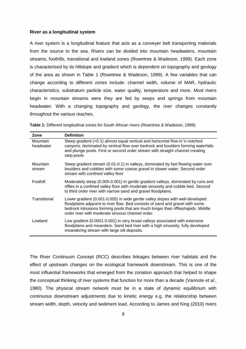
River as a longitudinal system

A river system is a longitudinal feature that acts as a conveyer belt transporting materials

from the source to the sea. Rivers can be divided into mountain headwaters, mountain

streams, foothills, transitional and lowland zones (Rowntree & Wadeson, 1999). Each zone

is characterised by its hillslope and gradient which is dependent on topography and geology

of the area as shown in Table 1 (Rowntree & Wadeson, 1999). A few variables that can

change according to different zones include: channel width, volume of MAR, hydraulic

characteristics, substratum particle size, water quality, temperature and more. Most rivers

begin in mountain streams were they are fed by seeps and springs from mountain

headwater. With a changing topography and geology, the river changes constantly

throughout the various reaches.

Table 1: Different longitudinal zones for South African rivers (Rowntree & Wadeson, 1999).

Zone Definition

Mountain headwater

Steep gradient (>0.1) almost equal vertical and horizontal flow in V-notched canyons, dominated by vertical flow over bedrock and boulders forming waterfalls and plunge pools. First or second order stream with straight channel creating step-pools.

Mountain stream

Steep gradient stream (0.01-0.1) in valleys, dominated by fast flowing water over boulders and cobbles with some coarse gravel in slower water. Second order stream with confined valley floor

Foothill Moderately steep (0.005-0.001) in gentle gradient valleys, dominated by runs and riffles in a confined valley floor with moderate sinuosity and cobble bed. Second to third order river with narrow sand and gravel floodplains.

Transitional Lower gradient (0.001-0.005) in wide gentle valley slopes with well-developed floodplains adjacent to river flow. Bed consists of sand and gravel with some bedrock intrusions forming pools that are much longer than riffles/rapids. Middle order river with moderate sinuous channel order.

Lowland Low gradient (0.0001-0.001) in very broad valleys associated with extensive floodplains and meanders. Sand bed river with a high sinuosity, fully developed meandering stream with large silt deposits.

The River Continuum Concept (RCC) describes linkages between river habitats and the

effect of upstream changes on the ecological framework downstream. This is one of the

most influential frameworks that emerged from the zonation approach that helped to shape

the conceptual thinking of river systems that function for more than a decade (Vannote et al.,

1980). The physical stream network must be in a state of dynamic equilibrium with

continuous downstream adjustments due to kinetic energy e.g. the relationship between

stream width, depth, velocity and sediment load. According to James and King (2010) rivers

10

follow the basic law of conservation of energy, rivers tend to a uniform expenditure of energy

along their lengths. The shape of a river is therefore a consequence of this uniform

expenditure known as stream power, a product of Slope (S) and Discharge (Q). There is a

direct relationship between S and Q, when S is high in the upper reaches the Q is normally

low, as the Q increases the S will decline to maintain the constancy of QS (Gordon et al.,

2004).

The RCC can be used to predict the changes in catchment topography, hydrology,

temperature and water chemistry between the headwater and the lowland which can then be

used to predict the longitudinal changes of a rivers production, input, transport, utilisation

and food storage (James & King, 2010). These changes will be notable in the river

communities.

The Riverine Ecosystem Synthesis (RES) view rivers as longitudinal arrays of large

geomorphological conditions that do not consist of a fixed sequence of downstream changes

but account for the more sensitive discontinuities in the typical sequence (Thorp et al.,

2006). Unlike the RCC their order of occurrence does not follow the downstream continuum.

The characteristics that influence the RES are physical and chemical, including tributary

confluence, divergence and convergence areas in braided channels and vegetated islands.

These characteristics form a template for ecological zonation.

The longitudinal organisation of river ecosystems can be distinguished through the

geomorphological classification of river reaches. A hierarchical framework proposed by

Frissell et al. (1986) has a spatial scale range from the catchment drainage network to a

single substratum particle as shown in Table 2. The hierarchical spatial scale is link to a

specific time scale: the highest hierarchical level changes over geological time were the

lowest hierarchical level is vulnerable to change over a small period of time like a day or

even hours and minutes.

11

Table 2: The hierarchical classification levels (Rowntree & Wadeson, 1999).

The hierarchical classification for South African rivers consists of six levels namely

catchment, zone, segment, reach, morphological unit and hydraulic biotope each describing

a different geomorphological feature of the river as depicted in Figure 3.

Figure 3: The South African hierarchical system (Rowntree & Wadeson, 1999).

The nature of features at each scale according to this hierarchical classification will be

determined by the nature of those units higher in the hierarchy. For example the reach unit

characteristics are either bedrock or free-forming in alluvial, this will determine the lower

units like the floodplains, sinuosity, substratum size etc. and thus the morphological

characteristics present in the next level (Ward, 1998). Rivers does not only consist of a

longitudinal dimension but also of vertical and lateral dimension which is temporal in nature.

Classification Description

Catchment The area draining into the stream network

Zone Areas within the catchment homogeneous in runoff and sediment production

Segment Section of channel corresponding to each zone through which flow of water and sediment are routed

Reach The length of channel within which the constraints on channel form are uniform so that a characteristic assemblage of channel forms occurs within identifiable channel patterns

Morphological unit The basic channel spanning structures comprising channel morphology, such as pools and riffles

Hydraulic biotope Small patches characterised by specific flow type sand substratum conditions

12

River as a vertical dimension

Surface and groundwater are hydraulically connected to each other in most areas, and

therefore surface water bodies are integral parts of groundwater flow systems. The surface

water can seep through unsaturated zones and still act as a recharge boundary for

groundwater (James & King, 2010). This interchange between surface and groundwater

allow contaminants to be transported from one source to another. The movement of surface

and groundwater is directly related to the geology and topography of the specific area, where

the climate, precipitation and vegetation affects the distribution of water on the surface.

There are many factors that can influence groundwater flow systems that include the

recharge volume from precipitation, geology, watershed characteristics, hydraulic conditions

and hydrogeological boundaries such as no-flow boundaries (Fisher et al., 1998). If the

piezometric surface are above that of the surface water of the river it can be defined as an

effluent system (gaining stream) and the groundwater will contribute and sustain the

baseflow, typical in periods of lowflow as shown in the first picture in Figure 4 (Malard et al.,

2002). In areas where the piezometric surface is below that of surface water the river can be

defined as an influent river and water will discharge from the river into groundwater as

shown in the second picture in Figure 4 (Malard et al., 2002).

Figure 4: Gaining and losing river systems. Water is either transported from the shallow aquifer into the river system (gaining stream) or water is lost from the river into the shallow aquifer (losing stream) (Stute, 2002).

The vertical exchange of material and energy between surface water and the river bed is just

as important as the transport of material longitudinally downstream and laterally between

floodplains and the main channel. Therefore it is important to link the groundwater ecology to

the traditional ecology of a river system (Malard et al., 2002). The hyporheic zone is

immediately below the riverbed at the boundary of surface runoff and groundwater, this flow

is called the hyperhoes. Particular organic matter accumulates in the hyporheic zone and are

temporarily retained before it is released back into the river system therefore the hyporheic

zone plays an important part in the nutrient cycle of a river system. The exchange of water,

13

nutrients and organic matter between groundwater and surface water can have major

influences on the temperature, nutrient source and the patchiness of organisms within

streambed sediment (Malard et al., 2002).

The lateral dimension within a river

The third component of river ecosystems is the lateral dimension where interaction between

terrestrial and aquatic ecosystems takes place when different parts of the river become

inundated at different times. These ecotones include backwater, riparian zone, riverine

wetlands and floodplains. This process is often referred to as the Aquatic Terrestrial

Transition Zone (ATTZ) and is dependent on seasonal fluctuations in flow and the

overtopping of river banks during periods of high flow (James & King, 2010). The drowned

vegetation creates a new aquatic environment where nutrients are released from terrestrial

vegetation. During this period of inundation large quantities of organic carbon and inorganic

nutrients are deposited onto floodplains leaving behind fertile soil for terrestrial vegetation. A

river system is more complex than just a channel from the source to the sea and in many

large rivers in Africa fish synchronise their reproduction to periods of high flow, with adults

migrating onto inundated areas to lay eggs. Fish larvae continue to feed and grow in these

rich inundated areas until they are strong enough to withstand the velocities of the main

channel and therefore it is important not to disturb the natural flows regime of a river system

(James & King, 2010).

The temporal nature of a river

The fourth component in river systems is a temporal one and the most important driving

factors are flow regime, sediment, chemical and thermal regime. The most important one of

these are flow regimes as it has the ability to affect all the others (Wohl et al., 2007). It plays

a distinctive role in driving ecosystem processes and is therefore commonly referred to as

the ‘master’ or ‘maestro’ physical variable (Walker et al., 1995).

Flow regime can be described as the daily, seasonal and inter-annual variation in flow and

its capacity to do work on the channel. Flow regime is largely responsible for the patterns in

channel form as well as fluctuations in biological communities including the composition

(kind of species present) and structure (proportion of different types of species) (Power et

al., 1988). It is also responsible for driving ecosystem processes such as the nutrient cycle

as well as evolutionary processes such as a species morphological behaviour and life history

adaptations to flood and drought.

14

2.3. Eco-hydraulics

Water in a river originates from the input of precipitation (P) to a catchment either as runoff

or stream recharge from groundwater and in turn produces streamflow and discharge (Q) as

output both varying in space and time (James, 2008). Variation of input will result in time-

varying hydraulic conditions (H), which can be described as the hydraulic characteristics of

riverine biota. Hydraulic conditions are determined by Q, channel form and instream

vegetation (flora); the river channel is determined by the geology and sediment supply,

hydraulic conditions and by instream flora; the instream flora is dependent on hydraulic

conditions and the river channel and the instream fauna depends on the hydraulic conditions

and on the river channel (Figure 5). Different inputs will affect the hydraulic conditions and

output of a river system.

15

Figure 5: Model of an ecohydrological system (James, 2008).

Different organisms can be linked directly to different flows for instance fish that migrate

upstream during periods of floods or spawn during small floods in the dry season. The

hydrological data on rivers inform us on discharge, the volume of water moving past a

defined point over a period of specified time (James & King, 2010). Hydrological data cannot

account for the forces acting on the channel or for the change of conditions at different

biotas and therefore hydraulic data is required.

Hydraulic data convert flow data into flow velocity, depth, level of inundation (area where

river floods its banks), stream power (ability to transport sediment) and more. The hydraulic

16

conditions of a water column differ, with the slowest flow at the river surface, bed and edges

increasing in velocity towards the centre of the column. Different riverine species live in a full

range of physical conditions and therefore it is important to understand hydraulic conditions

of river ecosystems for ecological studies.

“Hydrological data detail the magnitude, frequency, duration and timing of each kind

of flow over days, seasons, years and decades” (James & King, 2010).

“Hydraulics transforms this information into descriptors of the water-related

conditions experienced by each species over days, seasons, years and decades.”


The collection of hydrological data and the modelling thereof will provide predictions on how

many hydraulic habitats are available under various flow regimes for different species

specified by ecologists. Key linkages between river ecology and hydraulics are described in

the section that follows.

2.4. Flows and channel morphology

According to Heggenes (1996) the presence of a riverine species or community can be

compromised by a change in any one of its environmental components, physical, chemical

or biological. One of the key physical components is the hydraulic nature of the habitat and

to understand why riverine species live in these habitats has to define this aspect of habitat

in more detail. Through hydraulic modelling it is possible to predict changes in hydraulic

conditions within a river due to flow alterations and how this will affect the habitat of

species/communities (Hardy, 1998). Different fish species is dependent on different flow

condition for instance, species with a spawning preference for fast turbulent flow could be

expected to decline in numbers if flow is altered to consistently slower flow, and river

scientists need to be able to predict those conditions (Heggenes, 1996).

It is crucial to develop a database of information on the optimal hydraulic habitat of key

riverine species to predict how changing hydraulic conditions could affect the river

ecosystems (James & King, 2010).

2.5. River channels

River systems are dynamic and change constantly due to flowing water and sediment load

that works the river channel and bed. This work done by a river is responsible for

maintaining and eroding channel features such as banks, bars, pools, riffles, secondary

17

channels and islands (Rowntree & Du Plessis, 2003). The hydraulic features such as step-

pool formations in headwater and riffle-run sequences in foothill rivers are repeated through

its respective zones due to hydraulic conditions created by river flow. Different discharges

play different roles in the ecosystems of a river e.g. floods rip out new vegetation invading

main channels and wash them downstream to maintain channel width and its ability to

transport flood waters (James & King, 2010). Altering flows will move and sort alluvial

deposits on the riverbed in different ways and therefore create distinct patches of habitats

from sand particles to boulders, contributing to the biodiversity of organisms within a river

system.

Riverine species have to adapt to this dynamic geomorphological world to ensure their

survival, adult fish use deep pools and meander bends for resting areas where juvenile fish

use sandbars, slackwater and side channels to protect them against predators. Altering the

flow and sediment regime of a river will change the quantity and quality of available habitats

and may threaten the ecological integrity of the river ecosystem itself (Beck & Basson,

2003). The flows required for maintaining the river channel morphology can be referred to as

channel maintenance or flushing flows, in this document the term maintenance flow is used

since it covers a wider spectrum of features.

To understand the relationship between channel features and flow requires an

understanding of the balance between variables such as discharge, sediment size, load and

river slope and how they interact through time. To identify the flows responsible for channel

maintenance is beyond the scope of this study and requires a combination of expert

judgment and examination of major breaks in the cross-sectional channel shape, floodplain

height, vegetation zones and flow frequency. To assess the direct influence of hydraulic

changes in a river on aquatic organisms three different approaches have been used in South

Africa namely: Habitat Suitability Criteria (HSC), Hydraulic Biotopes and Flow Classes.

Sediment movement and sorting

River flow can act directly on organisms through the force of velocity and volume or indirectly

through sediment transport, depositing or sorting sediment on river beds which forms an

important component of river habitat.

Different flows in a channel perform different types of work such as: eroding, transporting,

sorting bed sediment, building sandbars etc. A key aspect of ecohydraulics is to identify

which flows perform these functions and how this will change by altering flow regimes. The

18

movement of fines in a channel during floods is natures’ way of disturbing invertebrates and

algal populations.

Habitat time-series

Rivers are dynamic bodies that change constantly over a period of time and ideally hydraulic

studies should integrate some habitat time-series analysis because the well-being of any

organism depends on the past and present habitat availability and not only on the immediate

availability (Orth, 1987; Capra et al., 1995). To predict the impact that an alteration in flow

will have on river ecosystems, duration, frequency, timing of flows and time-series should be

components of any assessment of hydraulic studies. This should become a standard part of

scenario analysis to support management and sustainable development of river systems.

By combining hydrological data and hydraulic data in models it is possible to predict different

scenarios of flows for different discharges.

Habitat suitability criteria (HSC)

HSC is widely used by ecologists worldwide and was the first method to be tested in South

Africa (Arthington & Zalucki, 1998). HSC defines the most commonly used hydraulic habitat

by any selected species. It includes data of depth, velocity, substratum particle size and the

presence of species of interest in the river system.

Deriving HSC is time-consuming due to the fact that it should include the full range of habitat

conditions a species will encounter and therefore it is not feasible to derive a HSC for each

species within a river. One approach is to group species into habitat guilds and then choose

an indicator species for each guild. This is a complex study and different life stages of the

same species may have different hydraulic dependencies and therefore have to be treated

as different ‘ecological species’ (Hayes & Jowett, 1994). Very little work of this nature has

been done in South Africa and it is a topic that needs further investigation to manage future

flows to support the different life cycles of valued species.

Hydraulic biotopes

Hydraulic biotopes can be used to describe hydraulic habitats of different species. Rowntree

(1996) defines a biotope as “a set of relatively uniform physical and biological conditions,

together with the distinctive biological community associated with it”. Thus a biotope defines

a group of species (community) where habitat only defines the living condition of a specific

species. The hydraulic biotope concept was developed in South Africa by geomorphologists

(Rowntree & Wadeson, 1999) describing the physical properties of hydraulic biotopes and

19

ecologists (Rowntree, 1996; King & Schael, 2001; Pollard, 2001) defining their relevance for

different aquatic species in the Western Cape headwater streams.

Mapping of hydraulic biotopes can either be done by hand in the field or digitised later or the

hand drawn maps can be combined with digitised coordinates taken with a differential GPS

on-site. As discharges change the hydraulic conditions change and maps have to be

redrawn for hydraulic biotopes and cannot be predicted through modelled drawing (King &

Schael, 2001). Maps with measurements of velocity and depth at cross section points can be

overlain with hydraulic biotope maps to allow for statistical testing of depth, velocity and

hydraulic variables.

Flow Classes

Flow classes were initially developed by Oswood and Barber (1982) and later adapted for

fish habitats for South African rivers by Kleynhans (1999). Flow classes are broad categories

of hydraulic habitats described by key parameters such as depth and velocity.

Flow classes for fish

Predefined flow classes were determined by a panel of experts based on habitat

requirements of 134 indigenous species of freshwater fish. The following four flow classes

were pre-defined: slow-shallow (SS), slow-deep (SD), fast-shallow (FS), fast-deep (FD) and

include velocity, depth and type of flow (Table 3).

Table 3: Flow classes for fish and method of data collection (Kleynhans, 1999)

Class Velocity Depth Description Sampling Method

SS Slow <0.3 m/s

Shallow <0.5 m

Shallow pools and backwaters

Small seine, Electroshocking

SD Slow <0.3 m/s

Deep >0.5 m Deep pools and backwater Large seine, Cast net

FS Fast >0.3 m/s

Shallow <0.3 m

Shallow runs, riffles and rapids

Electroshocking

FD Fast >0.3 m/s

Deep >0.3 m Deep runs, Riffles and rapids

Electroshocking

These flow classes are a very broad description with flow-depths covering only four

categories and flow-velocity with only two categories that are important for fish (Figure 6).

These flow classes are widely used in assessments of South African Ecological Reserve and

Ecological Status. In recent studies Lamouroux et al. (1999) described five different velocity

20

classes for fish which lead to more defined flow classes and should be considered in future

monitoring.

Figure 6: The four velocity-depth flow classes used in this study (Kleynhans, 1999).

The complexity of understanding the biological responses and quantifying these ephemeral

phenomena presents considerable challenges for ecologists, geomorphologists and

hydrologists. Altering the flow of a river can either act directly on an organism or indirectly by

affecting its ecological habitat. Therefore, the relationship between flow and riverine biota

are studied by three different approaches: HSC, hydraulic biotopes and flow classes.

Hydraulic biotopes are not well understood hydraulically and therefore they are not

compatible with hydraulic models. HSC are compatible with hydraulic models and their

results are testable and predictive but detailed data collection has to be done over smaller

areas to make it cost effective and efficient. Flow classes are semi-quantitative meaning that

they can be applied on ‘best-available-knowledge’ and are compatible with a variety of

hydraulic models.

21

2.6. Eco-hydraulic modelling

The modelling in this study is focused on the linkage of hydraulic conditions with the

geomorphological and biological characteristics and the discharges that contributes to the

change. The need for modelling is to predict the change in hydraulic conditions, flow depth

and velocity and link them to organisms (fish). This is used for short-term description of

hydraulic habitat for organisms which are influenced by their environment and does not take

into account channel form, hydraulics and vegetation and therefore cannot be used for long-

term predictions that include the interaction of geology, sediment supply and vegetation


There are many various modelling approaches and models that can predict these

characteristics, with the main difference being the accuracy or resolution of describing

hydraulic habitat conditions. The two main types are empirical and deterministic. Empirical

models are based on the correlation of measured values of the different variables such as:

water level and discharge as opposed to deterministic models that describe the relationship

between variables and processes for example: the Saint Venant equation of mass and

moment can be described through the relation of depth and velocity (James & King, 2010).

Deterministic models will always include some empirical content that can be introduced

through equation coefficients and statistical representations to account for processes that

influence the relationships between variables which are not fully described. The more

detailed the input information, especially topographic survey data in a model, the higher the

resolution and the more realistic is the process description. The empirical models require

less input or system information but more discharge and flow data is required to provide a

basis for correlation between different variables. Therefore an empirical model that is

calibrated for a specific site will have greater accuracy, but the deterministic model will be

more general and have better transferability between sites (James & King, 2010).

The most basic description for river hydraulics is the relationship between stage and

discharge at a specific site. This is modelled by empirical correlation of measured discharges

vs. water level at the site and requires no physical site information. With less flow data and

more site data deterministic modelling can also be used to determine the relationship

between stage and discharge (James & King, 2010). To calculate cross-section average

velocities, deterministic modelling is required with the addition of some site surveyed data. At

areas where site information is severely limited the simplest approach is to assume uniform

flow conditions. By combining the one-dimensional continuity equation with a resistance

equation (presented in the next chapter) it is possible to find an appropriate model where

22

information requirements are limited to channel slope, cross-section geometry and a

resistance coefficient to account for channel characteristics. To model cross-section average

velocities along a reach of the river, a 1-D non-uniform flow model such as HEC-RAS can be

used. This is similar to uniform flow models except that it supports a number of cross

sections. The depth-average velocities of a river section can only be described as adjacent,

non-interacting sub channels and therefore for more accurate modelling other approaches is

required.

Depth and velocity distributions over a two dimensional area can be modelled either

empirically or deterministically. HABFLO use frequency distributions to describe the

occurrence of depth and velocities over cross sections or reaches in a system and requires

input information of channel and flow characteristics (James & King, 2010). HABFLO does

not show spatial arrangements but only indicates the relative abundance of hydraulic

conditions. This method suffers from the same scale limitations as the Froude’s and

Reynolds numbers in its hydraulic characterization although it is popular with some

ecologists, it is difficult to predict biotope arrangements with varying discharges without 2-D

deterministic modelling. River2D provides flow depth and velocity data that can be

interpreted in terms of spatial arrangement and abundance as necessary (Steffler &

Blackburn, 2002b).

Hirschowitz et al. (2007) reviewed the different hydraulic models and their application in

ecological reserve determination. With the wide variety of models available, considering

advantages and disadvantages, requirements, level of accuracy and precision as well as the

resources required and available information where taken into account. A high resolution

model (e.g. 2-D) is not necessarily better than a lower resolution model (e.g. 1-D). It is of no

use describing hydraulic conditions in higher resolutions than the available HSC can use and

therefore the review of Hirschowitz et al. (2007) shows that HEC-RAS is more than sufficient

for 1-D analyses and River2D for 2-D analyses for most eco-hydraulics applications. Both

these models are available from the internet free of charge. It is important to note that the

quality of a model is directly related to the input data, and the specification of resistance

within a system.

The empirical model is statistically derived from measured data at similar sites for frequency

distribution of velocity classes. The deterministic model is a simulation of flow by the Saint

Venant equations (James & King, 2010). The empirical model only describes the abundance

of flow classes and not their spatial distribution where the deterministic model represents

high resolution of spatial descriptions of velocity classes from which the abundance can be

23

derived (Figure 7). The empirical model accuracy depends on the representativeness of the

data used for compilation and only requires rough data for description of flow and bed

characteristics. The deterministic model requires detailed topographic surveyed information

for the particular site and allow for a more general output and can accommodate a wider

range of discharge inputs (James & King, 2010).

Figure 7: Empirical vs. deterministic modelling of hydraulic conditions.

HEC-RAS description

HEC-RAS was developed by the Hydrologic Engineering Centre of the U.S. Army Corps of

Engineers to perform one-dimensional calculations for natural or constructed channels. The

model solves the energy equation between cross-sections to calculate/generate water

surface profiles for steady and unsteady flows. HEC-RAS is widely used and accepted for

flood modelling and flow analyses across the world. The software has a graphic user

interface, separate hydraulic components, data storage and management capabilities.

In this study HEC-RAS (version 5.0.1) was used to route flows ranging from 1m3/s to

4000m3/s along the study area in the lower Thukela River. The program can be downloaded

from the following website: http://www.hec.usace.army.mil/software/hec-ras/

24

River2D description

River2D was developed by Professor Steffler at the University of Alberta, Canada and is a

public-domain two-dimensional depth average hydrodynamic model. The model consists of

four separate modules and is used in succession:

Table 4: Different modules used within the River2D model and their relevance to this study.

Model Description Applicability

R2D_Bed Is the most crucial factor in river flow modelling, representing the physical features of the river channel bed, including bed elevation and bed roughness height. The model is based on the TIN methodology, consisting of nodes and breaklines for spatial interpolation. The process involves the creation of a preliminary bed topography text file from surveyed data, and then editing and refining it in R2D_Bed before it can be used in the R2D_Mesh module.

Yes

R2D_Ice This module is equipped to model flow under ice cover of known geometry and calculations are done based on ice thickness and ice roughness height.

No

R2D_Mesh The resulting R2D_Bed file is used in R2D_Mesh for final refining and to develop a computational discretization and to set boundary conditions as input for River2D.

Yes

River2D River2D is then used to solve water depth and flow velocities and to visualize and interpret the predictions. River2D include colour maps, contour maps and velocity vector fields to aid in visualising the progression and/or final results

Yes

The model is intended for natural streams and rivers and accommodates supercritical and

subcritical flow transitions and wetted areas. In this study River2D (version 0.95) was used

for depth-velocity predictions and can be downloaded from: http://www.river2d.ca/

2.7. Fish as indicator species

Fish are one of the most commonly used ecological indicators and can be used to measure

key elements of complex systems without having to capture the full complexity of a specific

system (Whitfield & Elliott, 2002). The primary function of an ecological indicator is to

monitor and track changes within an ecosystem. The different indicators that are used in

aquatic environments are chemical, physical and biological measures (Whitfield & Elliott,

2002).

Fish are an important component of ecosystems that can contribute to the establishment of

the environmental water requirements (EWR) for the Thukela River. Fish is not only an

25

important species for ecological health but they are one of the most important food sources

for many communities in Africa (Whitfield & Elliott, 2002). As indicators of ecological health

fish has the following advantages as an indicator species:

Long-lived: therefore good indicators of long-term exposure impacts.

Ubiquitous: they can live in a wide range of aquatic habitats mostly due to their

mobility.

Extensively studied: a lot of research has already been done regarding their habits,

habitats and occurrences.

Diversity: live across a wide range of feeding habitats, reproductive traits and

communities can comprise of a range of species allowing for a greater tolerance to

environmental stressors.

Easily Identified: relative to other groups of aquatic biota, fish are easy to identify to

species level and can be done in the field.

Well-known: fish provide recreational opportunities and many species are familiar to

the general public.

Toxicity trends: data analysis from the presence or absence of certain species and

their growth rate can detect sublethal effects.

Conservation: by establishing sensitive species the conservation of one species can

allow for the protection of large diversities of other species.

Fish as indicators of ecological health and flow alterations in a river ecosystem are already

being used throughout the world. Fish have been shown as valuable indicators for the

evaluation of ecological flow requirements in a river system and in addition provide

protection for many other aquatic systems (Karr, 1981; Kleynhans, 1999). Fish can thus be

considered as an important component in the establishment of ecological flows for river

ecosystems throughout the world.

2.8. Significant elements of the flow regime

Instream flow studies main focus is to determine the low flow conditions required to maintain

ecological wellbeing of river ecosystems. The greatest competition between organisms is for

the limited amount of available water. The following aspects will influence the flow regime to

maintain particular instream values (Jowett et al., 2008):

Floods will determine the overall form of the channel, floodplain surface and

vegetation cover due to its alluvial nature in the Thukela River and can be described

26

as channel maintenance flows. Large floods have a major impact on river channels

and cause disturbances to the river ecosystem for a time period due to the

displacement of aquatic biota and destroyed habitats.

Freshes which is smaller floods and are contained within the channel that occur a

few times throughout the year with limited effects. They will flush and refresh the river

bed by removing silt and algal coatings from riverbed sediments and also mobilise

sediment in most parts of the river channel. Freshes are both positive and negative

for flushing and cleaning the river bed to disturbing parts of the ecosystem.

Low flows are one of the most important flow regimes and occur at times when there

is the greatest competition for water, the availability of habitat is at its lowest and the

ecosystem is under major stress. Low flows can help with the recolonisation of fish

and macro invertebrates after floods and the re-establishment of aquatic vegetation.

Flow variation, the continuous change in flow regime which is a significant

hydrological feature and should be maintained within a river ecosystem. Long periods

of flat-lining (constant flow) should be avoided.

2.9. Ecological flow assesment methods

To determine ecological flow requirements a lot of different methods can be used from a

quick rule-of-thumb assessment to detailed studies over a few years (Jowett et al., 2008). A

large number of different methods have been used in different studies and new methods

continue to be explored. In this study only the most appropriate method related to the data

and study area are described. There is no universally accepted method for all rivers and

streams and very little evidence of the success and failures of the different methods (Jowett

et al., 2008). The following methods were applied in this study:

Historical Flow Method

The Historical Flow Method is referred to as the standard setting and is based on historical

flow records. This is the simplest and easiest method to apply and is a desktop rule-of-thumb

method to determine minimum flows (Stalnaker et al., 1995). The historic method make use

of statistical analyses to specify a minimum flow, it can be the average flow, a percentile

from the flow duration curve or the annual minimum with an exceedance probability. An

example of percentiles usage is as follows:

27

that the flow should never drop below 30% of the mean annual low flow (MALF) or

that the average flow should be maintained at a flow above 80% of the MALF and

can be referred to as the level of maintenance (Jowett et al., 2008).

This method is used to maintain the flow within the historical flow range, or to avoid the flow

regime to deviate largely from natural flows. The assumption made by using the historical

flow method is that the ecosystem has adjusted to the natural flow regime and that any

reduction in the natural flow regime will cause a reduction in the abundance and diversity of

aquatic ecosystems (Jowett et al., 2008). In other words the biological response is related to

flow. The most well-known historic flow method is the Tennant 1976 method which specifies

10% of the average flow as the lower limit for aquatic life and that 30% of the average flow

will provide a satisfactory stream environment (Jowett et al., 2008). The Tennant method has

been adapted to a more recently modified method and its recommended minimum flows are

similar to those predicted by the IFIM (Crowe et al., 2004). The Tennant method can be

extended by incorporating monthly minimum flows as a percentage of monthly mean flows.

The Building Block Method (BBM) aims to maintain an ecosystem in its existing state and

ignores the chance of a system being enhanced by other than the natural flow regime (King

et al., 2000). This method considers the duration and frequency of high flows and the degree

of low flows and are best used when the linkage between ecosystem integrity and flow

requirements are poorly understood.

Habitat Method

The habitat method quantify the loss of habitat caused by changes in the natural flow regime

and will assist in the evaluation of alternative flow requirements. The aim of the habitat

method is not only to maintain the natural biota but rather to improve the physical habitat for

instream requirements of biota (Jowett et al., 2008). This method requires complex hydraulic

sampling as well as knowledge of the ecosystem; the method states that if there is no

available habitat for a specific species that species cannot exist. However it is not to say that

when habitat does exist that the species will be present in the study reach. Species

distribution can be influenced by other factors like drought and food sources therefore the

habitat method only predicts suitable habitat for species of choice (Jowett et al., 2008).

Biological data required for habitat methods is in the form of suitability (preference) curves

for each species and different life stages. The main preferences for fish are given in the form

of depth, velocity and substrate.

28

The results of an instream habitat analyses is therefore dependant on the habitat criteria

used and can change drastically according to different species (Jowett et al., 2008). If the

chosen species has a preference for deep fast flowing water the maximum habitat will only

be provided by relatively high flow and if the preferences are for shallow slow flowing water

the maximum habitat will be provided by low flows and decrease with an increase in flows.

The habitat method does not assume that the natural flow regime is optimal for all species

and treats each species preferences individually (Jowett et al., 2008). Environmental

changes like an increase in temperature can have different effects on the distribution of fish

species within a river but is not incorporated in this study due to the variability of temperature

as a parameter.

29

3. Materials and methods

3.1. Study area

The Thukela River in KwaZulu-Natal is South Africa’s second largest river with a catchment

area of 29 000 km2 that has aptly been named for its ferocity (Whitfield & Harrison, 2003).

Increasing demand for water related ecosystem services from the Thukela River catchment

have resulted in an increase in pressure on the structure and function of the system

(Whitfield & Harrison, 2003). The lower portion of the Thukela River and the associated

Thukela estuary have been characterised as an ecologically important region of the Thukela

catchment with various social and ecological values associated with the use of ecosystem

services (Lamberth et al., 2009). The lower portion of the Thukela River and associated

estuary provides habitat for unique species of marine migrant, estuarine and freshwater

species and acts as a conduit for many anadromic species that utilise the middle and upper

reaches of the Thukela River. According to the FRAI classification system the lower Thukela

River and estuary has both recently been established to range between a moderately

modified (Class C) and largely modified (Class D) state (Kleynhans, 2007). This suggests

that although key ecosystem processes are occurring, some structure and function aspects

of the ecosystem may be negatively impacted, as a result of altered water quality, quantity

and habitat (Lamberth et al., 2009).

Activities associated with ecosystem service use in the lower Thukela River include water

abstraction for domestic use, industries, agriculture, mining, recreation, waste water

treatment and road and rail networks. Many of these ecosystem users abstract water directly

or indirectly (via municipal abstraction works) from the Thukela, Emandeni, uMsunduze and

Amatikulu rivers and some of them release treated or partially treated effluent back into

these systems. The region above the Emandeni River outfall supports the Thukela-

Mhlathuze Bulk Water Transfer Scheme which is currently under construction

(commissioned in 2015). A major industrial activity in the area is the Sappi Tugela Pulp and

Paper Mill that has both extraction and discharge points in the same region of the Thukela

River. Sappi releases effluent directly into the Thukela River via an underground pipe

system, approximately 500m below the confluence of the Thukela and Emandeni Rivers.

Risk assessment previously carried out in the Thukela system revealed that the lower

Thukela River together with the Emandeni River is the areas at the greatest threat of

stressors affecting the ecosystem health.

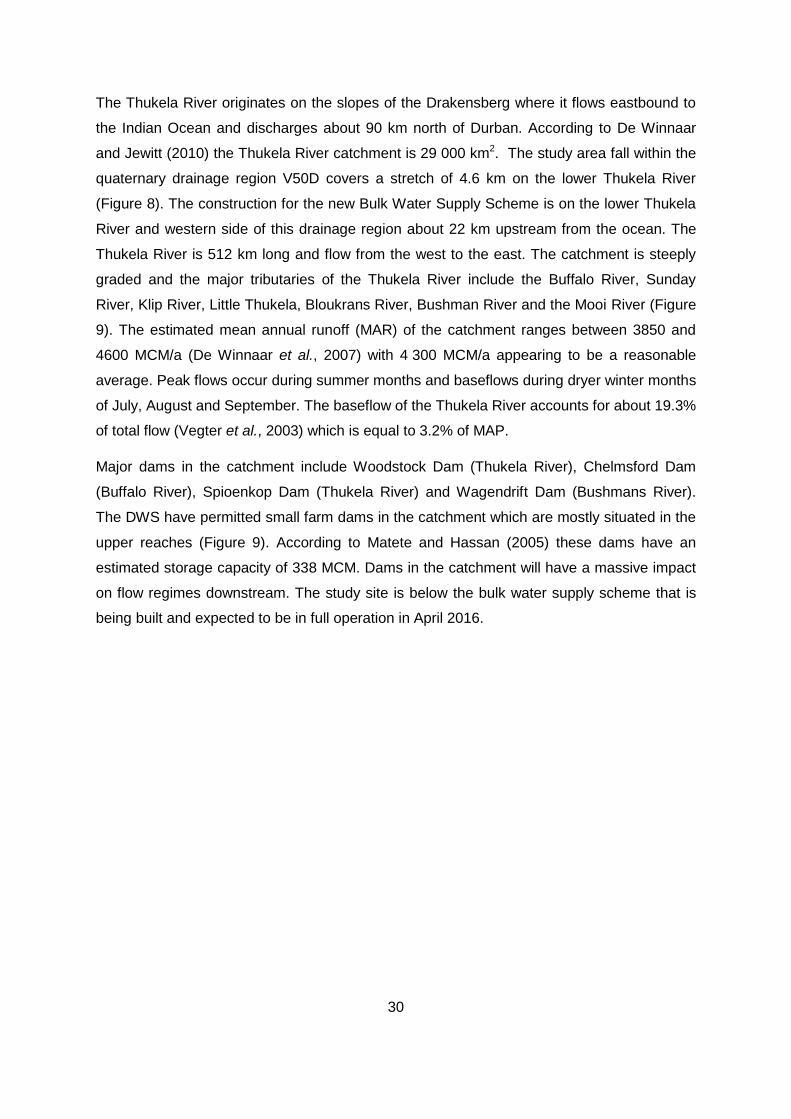
30

The Thukela River originates on the slopes of the Drakensberg where it flows eastbound to

the Indian Ocean and discharges about 90 km north of Durban. According to De Winnaar

and Jewitt (2010) the Thukela River catchment is 29 000 km2. The study area fall within the

quaternary drainage region V50D covers a stretch of 4.6 km on the lower Thukela River

(Figure 8). The construction for the new Bulk Water Supply Scheme is on the lower Thukela

River and western side of this drainage region about 22 km upstream from the ocean. The

Thukela River is 512 km long and flow from the west to the east. The catchment is steeply

graded and the major tributaries of the Thukela River include the Buffalo River, Sunday

River, Klip River, Little Thukela, Bloukrans River, Bushman River and the Mooi River (Figure

9). The estimated mean annual runoff (MAR) of the catchment ranges between 3850 and

4600 MCM/a (De Winnaar et al., 2007) with 4 300 MCM/a appearing to be a reasonable

average. Peak flows occur during summer months and baseflows during dryer winter months

of July, August and September. The baseflow of the Thukela River accounts for about 19.3%

of total flow (Vegter et al., 2003) which is equal to 3.2% of MAP.

Major dams in the catchment include Woodstock Dam (Thukela River), Chelmsford Dam

(Buffalo River), Spioenkop Dam (Thukela River) and Wagendrift Dam (Bushmans River).

The DWS have permitted small farm dams in the catchment which are mostly situated in the

upper reaches (Figure 9). According to Matete and Hassan (2005) these dams have an

estimated storage capacity of 338 MCM. Dams in the catchment will have a massive impact

on flow regimes downstream. The study site is below the bulk water supply scheme that is

being built and expected to be in full operation in April 2016.

31

Figure 8: The study area on the lower Thukela River.

32

Figure 9: Secondary and tertiary catchments of the Thukela system.

3.2. Climate

The range of climatic conditions is due to the vast area of the catchment. In the north and

west where winters are cold temperatures often fall below zero and frost occur regularly.

Summers are warm and temperatures often reach more than 35 °C. Along the cost and

relative to our study site temperatures are generally more moderate with smaller fluctuations

between winter and summer.

The mean annual precipitation (MAP) in the Thukela River catchment is 830 mm/a (Vegter et

al., 2003). With rainfall exceeding 1 000 mm/a along the escarpment and dropping down to

less than 600 mm/a east of Weenen. The central parts of the catchment receive between

600-800 mm/a where the coastal areas receive considerably more, in excess of 1 000 mm/a.

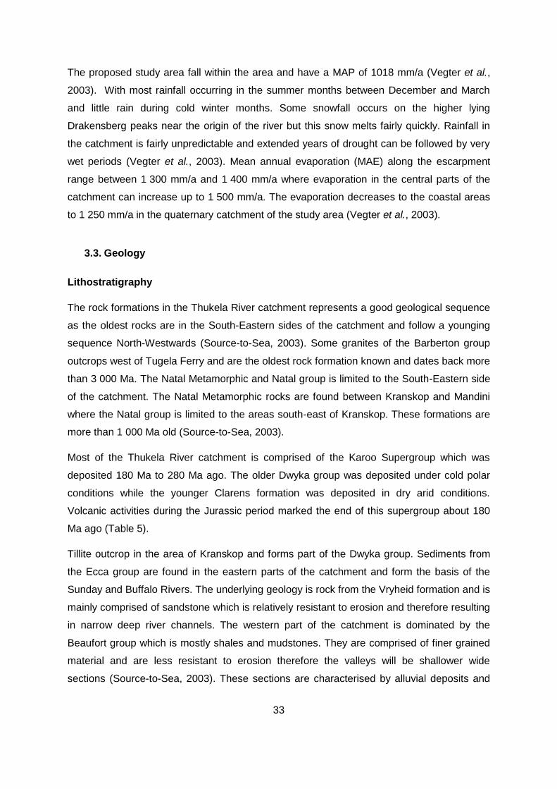
33

The proposed study area fall within the area and have a MAP of 1018 mm/a (Vegter et al.,

2003). With most rainfall occurring in the summer months between December and March

and little rain during cold winter months. Some snowfall occurs on the higher lying

Drakensberg peaks near the origin of the river but this snow melts fairly quickly. Rainfall in

the catchment is fairly unpredictable and extended years of drought can be followed by very

wet periods (Vegter et al., 2003). Mean annual evaporation (MAE) along the escarpment

range between 1 300 mm/a and 1 400 mm/a where evaporation in the central parts of the

catchment can increase up to 1 500 mm/a. The evaporation decreases to the coastal areas

to 1 250 mm/a in the quaternary catchment of the study area (Vegter et al., 2003).

3.3. Geology

Lithostratigraphy

The rock formations in the Thukela River catchment represents a good geological sequence

as the oldest rocks are in the South-Eastern sides of the catchment and follow a younging

sequence North-Westwards (Source-to-Sea, 2003). Some granites of the Barberton group

outcrops west of Tugela Ferry and are the oldest rock formation known and dates back more

than 3 000 Ma. The Natal Metamorphic and Natal group is limited to the South-Eastern side

of the catchment. The Natal Metamorphic rocks are found between Kranskop and Mandini

where the Natal group is limited to the areas south-east of Kranskop. These formations are

more than 1 000 Ma old (Source-to-Sea, 2003).

Most of the Thukela River catchment is comprised of the Karoo Supergroup which was

deposited 180 Ma to 280 Ma ago. The older Dwyka group was deposited under cold polar

conditions while the younger Clarens formation was deposited in dry arid conditions.

Volcanic activities during the Jurassic period marked the end of this supergroup about 180

Ma ago (Table 5).

Tillite outcrop in the area of Kranskop and forms part of the Dwyka group. Sediments from

the Ecca group are found in the eastern parts of the catchment and form the basis of the

Sunday and Buffalo Rivers. The underlying geology is rock from the Vryheid formation and is

mainly comprised of sandstone which is relatively resistant to erosion and therefore resulting

in narrow deep river channels. The western part of the catchment is dominated by the

Beaufort group which is mostly shales and mudstones. They are comprised of finer grained

material and are less resistant to erosion therefore the valleys will be shallower wide

sections (Source-to-Sea, 2003). These sections are characterised by alluvial deposits and

34

large alluvial floodplains. The fine grained minerals will be transported in suspension and

deposited in lower slow flowing sections like the study area section (Source-to-Sea, 2003).

Along the western edge of the Thukela River catchment post Beaufort sedimentary rocks are

found and are capped by Karoo-aged basalts. Dolerite dykes and sills of the Jurassic age

are found west of Kranskop (Figure 10). These features play an important role in the

geohydrology and help to understand the water properties in the study area.

Young unconsolidated sands are found only in the coastal area and are in the vicinity of the

lower Thukela River and estuary (King, 1997). This indicates the transport of alluvial sands

from upstream and then deposited in the lower sections. Some of these deposits can reach

a thickness of up to 40 m.

35

Table 5: Stratigraphy of the Thukela catchment (King, 1997)

Age (Ma) System Supergroup Group Formation Liothology

65 Quaternary

Tertiary Maputaland Calcereous sands

Cretaceous

Karoo

Zululand Marine siltstones, sandstones and some conglomerates

140 Jurassic Drakensberg Basalt

195 Lebombo Jozini

Letaba

Rhyodactite and rhyolite basalt

Clarens

Eliot

Nyoka

Ntabene

Molteno

Sandstone, Sandstone and mudstone, Mudstone interbedded with sandstone, Sandstone with subordinate mudstone, Sandstone, mudstone and shale

Triassic Beaufort

Tarkastad

Adelaide

Emakwenzini

Normandien

Sandstone with mudstone, Mudstone alternating with sandstone, Sandstone alternating with shale and mudstone, Sandstone interbedded with shale

Ecca

Volsrust

Vryheid

Pietermaritzburg

Shale and siltstone, Sandstone with some shale, Shale

345 Permian

Carboniferous Dwyka Tillite, Diamictite

Devonian

Silurian

Ordovician

Natal

Conglomerates, arkostic sandstone, Quarts-arenite and subordinate shale

570 Cambriam Natal Metamorphic Province

Mafic metavolcanic rocks with subordinate metasediments

3100 Pongola Nsuze

Tuffs, Black sandstone, Dactites and rhyolites, quartzites and shales, basalts and andesite, greywackes, conglomerates and shales

3200 Baberton Sequence

Swazian granites

Granite and granit gneiss

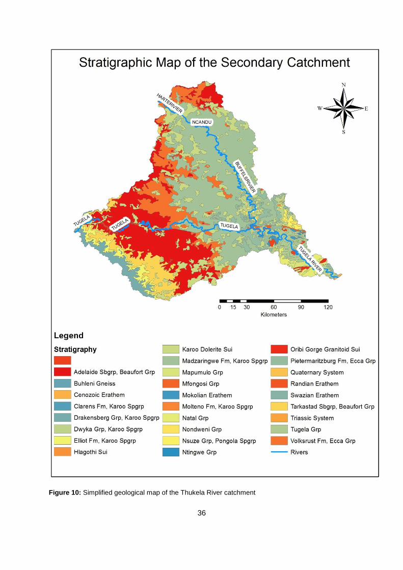
36

Figure 10: Simplified geological map of the Thukela River catchment

37

Tectonics

Parallel to the coast some 70 km inland a well-defined area has been faulted which led to

the development of tilted block faults, horst and garben structures in the study area south-

east of Kranskop (Source-to-Sea, 2003). These structures are of the post Karoo age and are

limited to the lower Thukela River. The Southern Thukela fault plays an important role in

defining the morphology and position of the river. The fault was caused by the break-up of

Gondwanaland and there are a few more throughout the primary catchment, they play an

important role in the water bearing properties of prevailing aquifers (King, 1997).

Population

The total population for the Thukela River catchment is approximately 1 570 000 and

dominated by rural areas. The population of the quaternary catchment V50D of the study

area is approximately 39 000 (Statistics, 2013). Most of the population live in Mandini and

are poor with a GDP well below the provincial average (BKS, 2001). The other towns in the

close vicinity are the Thukela and Thukela mouth.

Land use

The agricultural sector in the quaternary catchment includes sugar cane and stock farming.

Sappi manufacture paper in the immediate vicinity and have a discharge point at the higher

part of the study area (Source-to-Sea, 2003). Sappi and other manufacturing companies

discharge in the Mandini River which is a tributary of the lower Thukela River and fall within

the study area.

3.4. Hydrological Data collection

Prior to the field trip site 1, 2, 3, 4 and 5 were selected by using aerial and satellite

photographs (Figure 11) as well as some alternative sites in case one of the sites were not

suitable. Preferred sites from a hydraulics perspective consisted of a single channel, located

on a reach with constant gradient and channel cross-section shape (Figure 12D). There was

no hydraulic control downwards of the selected sites and the sites contained suitable habitat

for the biota of interest. The desktop site selection saved a lot of time searching for sites.

Some of the major issues on the Lower Thukela River are accessibility and safety

(crocodiles) (Figure 12C).

It is critical to obtain a detailed representation of bed topography for 1-D and 2-D hydraulic

modelling. Site benchmarks (Figure 12A) were established in August 2015 and an open

38

water hydraulic survey was conducted on the 15th of August when water levels were

constant. A total of 6 cross-sections were surveyed with a Total Station (Nikon D-50) (Figure

12B, F, G) in the study area as well as a longitudinal transect with a level logger and

Aquameter from the upstream boundary to the downstream boundary taking both location

and depth measurements (Figure 11). A supplemented bathymetric survey was conducted in

April 2016 which was supposed to be the high flow period, but due to the drought the stage

of the river was lower than the previous survey.

Figure 11: Data coverage on the lower Thukela River during this study.

39

Figure 12: A) One of the benchmarks installed in April 2015 on the first survey for a cross-section to get a stage discharge profile, B) Setting up the Total station to complete the cross section. C) One of the crocodile encounters at a cross-section profile, D) Showing a single channel for one of the cross-sections, E) Ntaki measuring flow velocities with the flow meter, F) Starting a cross-section close and working the way back, G) Testing the prism to make sure it works before starting the cross-sections.

40

3.5. Fish collection

Fish collection surveys were carried out to the lower Thukela River in variable flow period

including low flow (August 2015) and high flow (April 2016). Multiple fish sampling

techniques were used for the different habitat types available during each survey with some

precautions taken for safety against crocodiles. Different netting methods that were used

during the surveys included kick nets, seine nets, casting nets and fyke nets (Figure 13).

Other methods that were used were electrofishing and angling depending on the

characteristics of the river system (Figure 13). The seine nets were used in shallow pools

and backwaters sampling vegetated overbanks were the cast nets were mostly used in

faster flowing water like rapids and riffle habitats. In areas with sand as the main substrate a

medium size seine net 35 m long with a 1.2 m deep bag in the middle with 8 mm mesh size

were used for sampling larger specimens and a smaller seine of 7 m long with a 1 m deep

bag with 1 mm mesh size were used for capturing small specimens in vegetation and along

banks and backwaters. The electrofishing were used in wadable habitats and stunned fish

were collected with fine-meshed hand-held scoop-nets. Sampled fish were placed into

buckets of water until identification and measurements (SL and TL) were taken. Fish were

described and counted in the field to determine community structures for each species. For

each effort different habitat variables were described including depth (mm), velocities (m/s),

substrate distribution (Figure 14) and cover types and were then compared to fish

community structures for each sampling type. The velocities were measured with a Global

Water Meter (model FP211) that can only take readings in increments of 0.1 m/s, thus

velocity curves are not smooth and differ from velocities simulated.

41

Figure 13: Sampiling methods used for fish collection during surveys included: A) Seine nets, B) Casting net, C) Electrofishing and D) Scoop net

42

Figure 14: The different habitats used for the channel index substrate in the WUA calculations. A)

Silt, B) Sand, C and D) Gravel, E) Sand cover area, F) Bedrock, G) Vegetated overbanks

43

3.6. Data analyses

3.6.1. Field Measurements

Discharge was calculated by using the velocity-area measurement method based on the

velocity at 60% of the depth (James & King, 2010). At site 1 the depth was measured every

meter and for site 2, 3, 4 and 5 the depth was measured in 2 m intervals for practical

reasons. At each point where depth was measured a velocity reading was recorded (Figure

15). Cross sections are then divided into different sections each with their own velocity, and

discharge for each section are calculated and then added to obtain a total discharge (James

& King, 2010).

Figure 15: Velocity-area method based on the velocity at 60% of the depth (John, 2001).

To calculate discharge with the velocity-area method the following equation were used:

𝑄 = 𝐴𝑉

Where Q is equal to the discharge (volume/unit time e.g. m3/second), A is the cross

sectional area as governed by the stage of the river in (m2) and V is the average velocity of

flow (m/s).

Two ropes where strung across the river at the sites, one to hold the boat in place and the

other to survey in a straight line. The rope that was strung for the cross-section had

markings on every meter and by using a total station the cross sections where mapped out.

The points, cross-section gradient and water stage where recorded manually and processed

afterwards.

44

3.6.2. DEM and cross sections generated

Elevation data in the form of 5 m contour lines, spot heights and bathymetric data from

surveys where merged to create the most accurate DEM (Digital Elevation Model) in ArcGIS.

The following steps were followed as a quality control to ensure data accuracy:

• All data sets were inspected and suspect values were removed.

• Bathymetric data were sorted by depth and those outside reasonable bounds were

removed.

• Unrealistic velocity data were removed.

The data where projected to UTM zone 36S (Universal Transverse Mercator) and a TIN

(Triangulated irregular network) where then created to get the most suitable 3D model of the

topography as suggested by the Hydrological Engineering Centre. LIDAR elevation data

were not available for the study. HEC-GeoRas with a series of tool was used to develop

geometric data for HEC-RAS which included stream centreline, main banks, flow paths and

cross sectional cut lines perpendicular to flow direction.

Cross sections generated by HECGeo-RAS from the DEM in GIS were imported into HEC-

RAS. The cross-sections were extracted from HEC-RAS at the same coordinates as cross

sections done with the total station and compared to estimate the accuracy of the newly

generated cross sections.

3.6.3. Model selection

The study area is 4.6 km long and for this study two hydraulic models were chosen (HEC-

RAS and River2D) to conduct the analyses and stimulate flow predictions.

HEC-RAS is a 1-D model and was used to generate estimate water levels for

selected flow modelling scenarios at the downstream boundary of the River2D

model. The reasons for selected HEC-RAS to assist in modelling are:

o By using HEC-RAS to predict downstream boundary water levels for River2D

will eliminate/minimize any boundary effects in River2D (Payne et al., 2011).

o HEC-RAS will assist in the calibration process of River2D based on the

relationship between Manning’s roughness and the roughness height.

River2D can accommodate dry elements under a wide range of flows under open

water conditions. River2D also have a fish habitat component, based on the

Weighted Useable Area (WUA) which is an important aspect of the study conducted.

45

The model will be used to simulate flows ranging from low flow (1 m3/s) to high flows

in excess of (1000 m3/s).

3.6.4. HEC-RAS analyses

Historical data from gauging station V5H002 (Mandini) were used to select 23 simulated

flows for various possible discharges of the Thukela River including drought, normal and

high flow periods. This is the closest gauging station to the study area and is situated 4.6 km

upstream from the first cross-section.

HEC-RAS was developed by the Hydrological Engineering Centre of the U.S. Army Corps of

Engineers (Brunner, 2001) to calculate water surface elevation by solving the energy

equation between cross-sections along a river section. The HEC-RAS model was set up

using surveyed river cross-sections and cross-sections generated from the DEM. The model

was then calibrated based on the measured open-water stage and discharge (4.3 m3/s) data

from the survey in April 2016. HEC-RAS was used to conduct the 23 model runs for various

selected discharges ranging from 1 m3/s to 4000 m3/s under open water conditions. The

water levels predicted by HEC-RAS were used as the downstream boundary conditions of

the River2D model (Payne et al., 2011).

3.6.5. River2D data analyses

The existing DEM created in GIS were used for topographic data in River2D. The

bathymetric data from the survey in August 2015 and April 2016 were used and integrated

as accurately as possible with the limited funding and equipment. Site information (e.g.

vegetation, geology, soil and bed material) were collected on the various surveys.

The river bed topographic data from the integrated DEM and the bathymetric data from

surveys as well as additional cross-section data generated with HEC-GeoRAS were used to

produce the bed file required by the River2D model.

Mesh generation

An appropriate mesh system is required to ensure numerical stability and accuracy in the

River2D model. One mesh profile was generated for flows in the study area, due to the

nature of the river which include high banks and minimum floodplains along the study reach.

A mesh system was generated using triangular finite elements for the River2D model. The

following features are present:

A computational domain was defined by exterior boundaries for the study area of

interest.

46

Breaklines were assigned at areas with significant topographic changes for example:

top and bottom of river banks.

The mesh grid size was set to 8 m for the main channel and refined to 5 m along the

river banks.

Areas of the mesh system were optimized by editing nodes and grid connections to

improve the quality index (QI) until a satisfactory value of greater than 0.15 was

obtained. A QI of 0.15 is considered to be acceptable for River2D modelling (Steffler

& Blackburn, 2002a).

The final mesh profile consisted of approximately 18258 nodes and 34625 finite

elements with an optimized QI value of 0.224.

Roughness height selection

The bed roughness height Ks (m) is an important aspect for River2D modelling. The

observation of bed material, land formation and vegetation provided a physical basis for

selecting reasonable initial values of bed roughness. The river bed consisted mostly of fines

(sand and some silt) with very little cobbles. The particle size of bed material D50 is 0.2 mm

(for sand and silt) with a typical Ks value ranging between 0.006 to 0.1 m according to the

(hydraulic and geomorphic characteristics of rivers in Alberta (Kellerhals et al., 1972)). Final

adjustments of Ks values were made during model calibration.

Boundaries

For this study discharge was assigned as the upstream hydraulic boundary and water level

was assigned for the downstream boundary. A total of 23 simulated flow scenarios were

identified and used for discharges ranging between 1 m3/s to 4000 m3/s, the same value set

used in HEC-RAS simulations. The corresponding water levels generated by HEC-RAS

were set as the downstream boundary for the River2D model.

Model Calibration

The River2D model was calibrated for open-water low flow conditions. A measured

discharge of 4.3 m3/s and water levels from the April 2016 survey were used for initial model

calibration. The primary model parameter for River2D is the roughness height. To select

suitable Ks, site information, bank and bed material, vegetation cover and literature reviews

of similar river systems have to be considered. The Ks was then adjusted until a satisfactory

match was obtained between the measured and simulated water levels, and were then

further adjusted based on the comparison between simulated and measured velocity profiles

along the study reach.

47

Calculating fish habitats

After calibration the River2D model can be used to calculate fish habitat index or availability

by making use of WUA using the same concept as in the Physical Habitat Simulation

System (PHABSIM) (Paxton, 2008). A composite suitability index (CSI) is used in the

calculation of WUA at each node in a specific domain and the area associated with that node

(CSI x surface area), CSI is dimensionless and therefore the unit of WUA will stay m2

(Paxton, 2008). To calculate WUA in River2D, data such as habitat Suitability Index (SI),

channel index, depth and velocity is required. SI is in the form of fish preference files

containing SI curves in table form for channel index, depth and velocity. River2D calculates

the product of these indices to obtain a CSI (Paxton, 2008).

Composite SI = depth SI x velocity SI x Channel Index

This file is then imported into River2D and combined with the channel index to calculate

WUA. Channel index can be described as a constant assigned for each computational node

that does not change with a change in flow such as the different substrates found in river

channels (Table 6) (Paxton, 2008). The bed topography editor, in River2D can be used to

build the computational mesh used for the channel index file by replacing the bed roughness

values with channel index values and later renaming them to the specific substrate and

changing the file extension from (.bed) to (.chi). Once the solution has converged to steady

state, with a goal solution change of less than 0.00001 and a reasonable inflow and outflow

value within 1% of each other the model will provide depth and velocity suitability indices for

each node over the entire computational mesh (Steffler & Blackburn, 2002a)

Table 6: Numbers assigned for different substrates on the computational mesh.

Channel Index Substrate

1 Silt

2 Sand

3 Small Gr.

4 Lg. Gravel

5 Cobble

6 Cobble 2

7 Boulder

8 Boulder 2

9 Bed Rock

10 Vegetated overbank

48

3.7. Ecological wellbeing of fish in the Thukela River

The following Lines of Evidence (LoEs) were used to characterise the ecological wellbeing

(or state) of the fish component of the riverine ecosystem in the study area:

o Statistical evaluation of shifts in community structure (Van den Brink et al., 2003;

O'Brien et al., 2009). The state evaluation were carried out using a multivariate

statistical procedure for fish community structures in relation to changes in

community structures (using a Redundancy Analysis ordination technique based on

Canoco version 4.5 software (Ter Braak & Šmilauer, 2002)). The direct correlation of

changes in fish community structures in terms of taxa obtained during surveys can be

interpreted and combined with Monte Carlo permutation testing to see if there are a

statistical significance between the relationship of community structures and

environmental variables (Van den Brink et al., 2003; O'Brien et al., 2009). With this

approach fish sample data and species ordination can be overlain with environmental

variables (such as habitat and velocity-depth) to acquire the drivers of shifts in fish

community structures in the lower Thukela River.

o Fish Response Assessment Index (FRAI) classification system and an adapted

method of FRAI was used in this study as shown in Figure 16 (Kleynhans, 2007).

Data that were required for fish habitats for addition to our database were used

including:

Velocity-depth preference data

Flow preferences

Substrate preferences

Importance and distance of fish migration

The FRAI approach incorporates the motivation for specific selections of, and use of

preference conditions. The FRAI results in two scores, an automated score and an adjusted

score (Kleynhans, 2007). The automated scores are largely based on the automated

evaluation of the state of the driver variables (FRAI metric variables) based on the

differences in expected and observed species in the assessment. FRAI allows operators to

manually evaluate the state of driver variables (selected physical environmental variables),

therefore the FRAI scores can be adjusted for the state of fish communities in response to

selected driver variables. The FRAI scores can be compared with the ecological

classification system, a continuum of six classes used in the Ecostatus methodology

(Kleynhans et al., 2008).

49

Figure 16: Comparisons/overlaps in scoring systems of the Lines of Evidence used in the study to

represent fish health (FRAI), community structures and community wellbeing.

3.7.1. Response of communities to habitat variable condition alterations

The following Line of Evidence (LoEs) was used to characterise the ecological flow

requirements of fishes in the study area:

o Indicator species recruitment information (Paxton et al., 2013).

o Fish Invertebrate Flow Habitat Assessment Index (FIFHA).

FIFHA was developed to evaluate the effects of flow dependant habitat type alterations on

an ecological indicator fish species and/or guild. FIFHA is an excel based evaluation tool

developed by Kleynhans (2007). The FIFHA integrates historical hydraulic data from weirs

with those collected during field surveys. The evaluation process includes:

o Practitioner must have a thorough understanding of the species/guild and their range

of habitat preferences for velocity, depth and available habitat. The specific use of

rheophillic or semi rheophillic species should be identified for different flow periods

(high or low flow). The assessment can be based on habitat suitability of species

and/or guild and the operator can modify the preference information to generate a

hypothetical flow-habitat preference which can be imported into River2D. For the

Thukela River two different species will be used to calculate a combined EWR to

maintain critical baseflow and still maintain the necessary diversity. Labeobarbus

natalensis will be used as a rheophillic species, they have a high preference for flows

and will mostly be used for velocity-depth classes, E. fusca is a lowland river species

that needs estuarine habitats for survival and can be considered an important

species to maintain diversity within the ecosystem. There is a relatively good

understanding of the biology and ecology of both species.

50

3.7.2. Habitat preference assessment

Velocity readings were taken 3 times at the different places with a transparent velocity head

rod (TVHR) for each effort where fish have been caught. The TVHR were inserted with the

flat side perpendicular to the flow and data were recorded in centimetres with the first

reading on the upstream side were water push up against the TVHR and the second reading

at the downstream side (Fonstad et al., 2005). The head difference between the two

readings were used to calculate the velocity for each reading and then divided by three to

get an average for that area. This was done three times and an average of the three times

was then used as the velocity for the effort. The TVHR has a highly significant correlation of

0.94 when compared to a traditional AA current meter making it precise to almost 5%

(Fonstad et al., 2005). The following equation were used to convert head differences to

velocities (Fonstad et al., 2005):

V = 0.728 * ((2gh) 0.5) - 0.1126 m/s

Where g is the gravitational velocity which is a constant at 9.8 m/s and h is the difference in

head from the reading facing upstream and downstream on the TVHR in metres (Fonstad et

al., 2005).

The depth of each effort where fish have been caught were measured with the TVHR thin

side turned into flow and depth would be unaffected by the TVHR. Measurements were

taken three times for each effort and the average of these readings was used in data

analyses.

For each effort where fish have been caught the substrate type was recorded in percentage

covering the bed. If channel bed was covered by more than one substrate type the combined

percentages of covered area were estimated and recorded out of 100%.

Velocity, depth and substrate were recorded for each effort and each species separately on

data sheets in the field. A box and whisker plot was created for velocity and depth using

average velocity and depth for each species. The percentile function was then used to

calculate the 5th, 25th, 50th, 7th and 95th percentiles for velocity and depth. The 5th percentile

shows the lower end of the data of which only 5% of the population was caught in including

slower velocities and shallower depths. The 50th percentile represents the velocity and depth

of which 50% of the population preferred making this the biggest and most preferred habitat.

The 95th percentiles represent the higher end of data of which only 5% of the population

preferred, including the higher velocities and depths. For substrate a stack column graph

was used to demonstrate the preferred substrate for each species out of 100%. These

graphs were used to create a preference file for indicator species that were used in River2D

51

to calculate the WUA. For velocity the 25th, 50th and 75th percentile were assigned a value of

1 which is the most preferred velocity for the specific species. For faster velocities an 85th

percentile were calculated and assigned a value of 0.5, for the 95th percentile a value of 0.25

was assigned. For slower velocities a 15th percentile was calculated and given a value of

0.25 and for the 5th percentile a value of 0.1 was given which is the least preferred habitat

type for velocities.

A preference file for depth for each species were created using the same techniques but it

was assumed that an increase in depth would relate to an increase in preference for any

given species and that the maximum depth is not the limiting factor but rather the minimum

depth and therefore the 50th, 75th, 95th percentile were all given a value of 1 and the 25th and

5th percentiles were assigned 0.5 and 0.1 respectively.

The stack column graph already calculated the preference for each species as a percentage

and these values were converted to a value out of 1 and assigned to each substrate type.

The preference files were saved as text delimited from excel and then changed to a (.prf) file

extension to be imported to River2D for calculations.

3.8. Historic method for calculating ecological flow requirements

The flow-duration curve were calculated on daily average flow data from 1963 to 2016, with

some data removed or edited according to missing information in data received from the

Department of Water and Sanitation. The indices used for flow duration curves are referred

to using a Qx notation when the x indicates the percentile that was used. Q50 is the median

monthly flow and represent the flow which exceeded 50% of the time, this method was

developed by the New England U.S. Fish and Wildlife service for catchments with good

historic hydrological records (Caissie & El-Jabi, 1995). The method is now slightly adapted

and used on a more seasonal basis to describe the median flow for 6 different seasonal

periods and is referred to as the New England Aquatic Base Flow method (ABF). The

different time periods are (Linnansaari et al., 2012):

Summer (January 1 to march 15) = to the February Q50

Autumn (March 16 to May 15) = to the April Q50

Early winter (May 16 to June 30) = to the June Q50

Winter (July 1 to September 15) = to August Q50

Spring (September 16 to November 15) = to October Q50

Early summer (November 16 to December 31) = to December Q50

52

The Q50 do not describe the environmental flow that needs to be maintained but indicates

the level of flow were no further abstraction of water is allowed and the actual minimum

environmental flow is determined by using a percentage of the natural flows where 70% of

the median flows as recommended by Fisheries and Oceans in Canada (Caissie & El-Jabi,

1995).

The Tennant method has also been used which specifies 10% of the average flow as the

lower limit for aquatic life (critical base flow) and that 30% of the average flow will provide a

satisfactory stream environment (base flow) for ecological survival. To increase the

ecological state of the river a flow of 50% (median) monthly flow is described and for freshes

70% were used, this is the flow that will flush bed sediment (Tennant, 1976).

3.9. Instream flow incremental methodology

There is no clear point at which instream conditions turn good or bad, but rather a general

assumption that habitat gets worse as flows decrease below optimal value. The rate of

habitat change vary with flow and therefore when habitat modelling results are available the

rate of change is used as the basis for setting a minimum flow. The point of greatest change

in the rate (the breakpoint) is used as the minimum flow requirement for the lower Thukela

River. This is set based on the criteria that higher flows will have a diminishing effect on

habitat availability although the effect of higher than optimum flows will be less significant to

those of decreasing the flow and any habitat loss may be balanced by the amount of cover

and food production (Jowett et al., 2008).

Instream flow incremental methodology (IFIM) can be described as hydraulic habitat

modelling and is a combination between habitat suitability and hydraulic modelling of the

river flow, also known as instream habitat modelling or physical habitat modelling. The river

uses physical habitat velocity, depth and substrate and in this study River2D was used to

predict the physical habitat based on the PHABSIM concept of WUA (m2/m) (Jowett et al.,

2008). The purpose of predicting the minimum flows are to maintain, or even improve the

physical habitat by retaining adequate water depth and velocities.

53

4. Results and Discussion

4.1. Digital elevation model (DEM) creation, predicting water levels and velocity-

flow classes

During the different surveys bathymetric data were collected by means of cross-sections and

random sections that were mapped with a Total Station. These data were combined with 5 m

contours and spot heights in ArcGIS to create an accurate DEM (Figure 17).

Figure 17: Topographic data used to generate a DEM.

Additional data were needed for the bed topography and therefore HEC-GeoRAS were used

to generate extra cross sections through the study area. The DEM created in GIS with 5 m

contours and spot heights were used as a topography map to delineate flow boundaries,

river banks and flood plains (Figure 18).

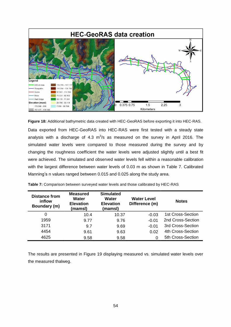
54

Figure 18: Additional bathymetric data created with HEC-GeoRAS before exporting it into HEC-RAS.

Data exported from HEC-GeoRAS into HEC-RAS were first tested with a steady state

analysis with a discharge of 4.3 m3/s as measured on the survey in April 2016. The

simulated water levels were compared to those measured during the survey and by

changing the roughness coefficient the water levels were adjusted slightly until a best fit

were achieved. The simulated and observed water levels fell within a reasonable calibration

with the largest difference between water levels of 0.03 m as shown in Table 7. Calibrated

Manning’s n values ranged between 0.015 and 0.025 along the study area.

Table 7: Comparison between surveyed water levels and those calibrated by HEC-RAS

Distance from inflow

Boundary (m)

Measured Water

Elevation (mamsl)

Simulated Water

Elevation (mamsl)

Water Level Difference (m)

Notes

0 10.4 10.37 -0.03 1st Cross-Section

1959 9.77 9.76 -0.01 2nd Cross-Section

3171 9.7 9.69 -0.01 3rd Cross-Section

4454 9.61 9.63 0.02 4th Cross-Section

4625 9.58 9.58 0 5th Cross-Section

The results are presented in Figure 19 displaying measured vs. simulated water levels over

the measured thalweg.

55

Figure 19: The comparison between HEC-RAS simulated water levels and measured water levels

along the thalweg after calibration with a discharge of 4.3 m3/s.

The correlation between measured and simulated water levels was determined for the

calibration in HEC-RAS to illustrate the relationship and accuracy of the model (Figure 20).

This is important as it proves that the model is truly calibrated and that the data used for

further analyses is trustworthy. The correlation coefficient for measured vs. simulated water

levels is 0.99 showing a strong linear relationship between the measured and observed

values.

Figure 20: Correlation between measured and simulated water levels at different cross-sections

using HEC-RAS after model calibration.

7.5

8

8.5

9

9.5

10

10.5

11

11.5

12

0 500 1000 1500 2000 2500 3000 3500 4000 4500 5000

Wat

er

Ele

vati

on

(m

amsl

)

Distance from inflow boundary (m)

Observed vs Simulated Water Level

Observed W.L. Simulated W.L. Thalweg

R² = 0.999

9.5

9.6

9.7

9.8

9.9

10

10.1

10.2

10.3

10.4

10.5

9.4 9.6 9.8 10 10.2 10.4 10.6

Me

asu

red

Wat

er

leve

l (m

amsl

)

Simulated Water level (mamsl)

Correlation between Measured and Simulated Water Level

Measured vs. Simulated W.L.

56

After HEC-RAS were calibrated with a 4.3 m3/s discharge, peak flow data were collected

from gauging station V5H002 (Mandini) and different discharges were selected ranging from

low flow to extreme floods for steady flow analyses. The model was then used to predict

water surface elevations at each cross-section according to the selected flows (Table 8). The

discharge ranges were selected to present the best stage-discharge curve. Only water levels

from the outflow boundary (end of study reach) were recorded to predict outflow conditions

in River2D.

Table 8: Predicted Water Levels by HEC-RAS for the River2D Model Downstream Boundary.

Model Run (I.D.)

River Flow (m3/s) Predicted water levels by HEC-RAS model (mamsl)

1 1 9.57

2 4.3(model calibration) 9.58

3 15 9.60

4 30 9.63

5 45 9.68

6 60 9.78

7 100 9.94

8 200 10.14

9 300 10.32

10 400 10.47

11 500 10.61

12 600 10.74

13 700 10.87

14 800 10.98

15 900 11.1

16 1000 11.21

17 1250 11.46

18 1500 11.7

19 1750 11.93

20 2000 12.13

21 2500 12.52

22 3000 12.86

23 4000 13.69

Figure 21 shows the stage-discharge curve simulated for the downstream boundary by HEC-

RAS for River2D. A linear interpretation between predicted water levels represents the

relationship between stage and discharge and can be used to extract any water level at any

given discharge for the downstream boundary of the study area (Figure 21). Water surface

elevations (mamsl) from the stage-discharge curve simulated by the calibrated HEC-RAS

model were used as a downstream boundary condition for the River2D model.

57

Figure 21: Stage vs. Discharge simulated from HEC-RAS model for the lower boundary conditions in

River2D.

4.2. River 2D

Bathymetric data collected from the two surveys, HEC-GeoRAS data from GIS and

topographic data from the DEM were used in the bed creation file for River2D. Breaklines

were assigned for areas of significance topographic change including upper and lower banks

and drop-offs. The thalweg (deepest section of a river channel) were defined as a breakline.

No-flow boundaries were delineated in an anti-clockwise direction and instream boundaries

in a clockwise direction. Everything to the left of assigned boundaries fall within the domain

and everything to the right fall outside the domain and does not form part of the channel and

act as a no flow boundary. The model were triangulated and exported as a mesh file and

could then be refined in the mesh section of River2D. A mesh grid was generated with

regional fill of 8 m in channel and 5 m along the banks. Nodes and bad triangles were

identified and edited until a satisfactory QI of 0.224 were obtained. The inflow boundary was

set at a discharge of 4.3 m3/s and the outflow boundary to 9.58 mamsl before the Mesh file

were exported as a .cdg file and imported into River2D were a steady flow analysis were

performed. Due to some irregularities in data the model did not merge. By filtering the data in

the bed program two points with unrealistic elevation heights were discovered in the river

channel and after they were removed from the data the new model merged with a goal

solution change of 0.00000024 and an inflow-outflow difference of less than 1%. To calibrate

9

10

11

12

13

14

15

0 500 1000 1500 2000 2500 3000 3500 4000 4500

Wat

er

Ele

vati

on

(m

amsl

)

Discharge (m3/s)

Stage-Discharge curve

Stage-Discharge curve

58

the model steady state conditions were considered and surface water elevation data were

extracted at each cross-section. The surface water elevation between measured data and

those simulated in River2D were compared. In areas were simulated water elevations were

too high a lower roughness coefficient were assigned and in areas were simulated water

elevation were too low the roughness coefficient were increased. This process was repeated

until a satisfactory fit were obtained with the largest differences between simulated and

measured water levels reaching as low as 0.07 m (Table 9).

Table 9: Comparison between surveyed water levels and those calibrated by River2D at a discharge

of 4.3 m/s.

Distance from inflow

Boundary (m)

Measured Water

Elevation (mamsl)

Simulated Water

Elevation (mamsl)

Water Level Difference (m)

Notes

0 10.40 10.38 0.02 1st Cross-Section

1959 9.77 9.83 -0.06 2nd Cross-Section

3171 9.70 9.76 -0.07 3rd Cross-Section

4454 9.61 9.60 0.00 4th Cross-Section

4625 9.58 9.58 -0.01 5th Cross-Section

Observed and simulated water levels were plotted against each other over the thalweg to

provide a graphical image of how well the model is calibrated (Figure 22).

Figure 22: The comparison between River2D simulated water levels and measured water levels

along the thalweg after calibration with a discharge of 4.3 m3/s.

7.5

8

8.5

9

9.5

10

10.5

11

11.5

12

0 1000 2000 3000 4000 5000

Wat

er

Ele

vati

on

(m

amsl

)


Observed vs Simulated Water Level

Observed W.L. Simulated W.L. Thalweg

59

The correlation co-efficient between measured and simulated water levels were determined

for the calibration in River2D to illustrate the relationship and accuracy of the model (Figure

23). This is important as it proves that the model is truly calibrated and that the data used for

further analyses is trustworthy. The correlation coefficient for measured vs. simulated water

levels is 0.98 showing a strong linear relationship between the two variables.

Figure 23: Correlation between measured and simulated water levels at cross-sections using

River2D after model calibration.

Simulated velocities were compared to those measured on surveys to assess the similarity

in magnitude and distribution on the cross-sections. The simulated velocities match closely

with the measured velocities along all cross-sections at the calibrated discharge and

therefore no further adjustments were required. In the section that follows banks are

described as left and right, looking downstream. The Global Flow meter can only measure

velocities in increments of 0.1 m/s and thus resulted in a difference between measured and

simulated velocity predictions. Discharge at each cross-section was calculated to get an

average discharge over the study area (Table 10).

Table 10: Discharges of sites using velocity-area method (Coordinates is in UTM 35s).

X Y


Discharge

Site 1 344716.484 6772217.231 0 4.29

Site 2 347112.980 6771781.484 1959 4.41

Site 3 348404.309 6771485.329 3171 4.22

Site 4 348645.591 6771073.928 4454 4.35

Site 5 348683.746 6770930.132 4625 4.24

R² = 0.9884

9.5

9.6

9.7

9.8

9.9

10

10.1

10.2

10.3

10.4

10.5

9.4 9.6 9.8 10 10.2 10.4 10.6

Sim

ula

ted

W.L

. (m

amsl

)

Observed W.L. (mamsl)

Correlation between Measured and Simulated Water Level

Simulated W.L.

60

Site 1: Cross-section

Site 1 was selected to be the inflow boundary and therefore marking the beginning of the

study area. The benchmark for the total station was placed on the right bank on higher

ground (Figure 21A). Beyond the benchmark the bank flattened and sugarcane plantations

are dominant. Habitat/substrate consists of very course gravels and small boulders (Figure

24D) on the right bank and changed into sand substrate from about 4 to 5 m all the way to

the other bank. This is a single channel with an isolated pool close to the left bank as shown

in Figure 25. The left bank is steep and consists mainly of solid rock. The area-velocity

method was used to calculate discharge and a Total Station was used to get elevation data

as accurately as possible (Figure 24A).

Figure 24: Site 1: cross-section, the inflow boundary for River2D A) Total station setup, B) View

across river, C) View upstream, D) View downstream.

61

Cross-section 1 is shallow with depths reaching a maximum of 0.95 m and velocities stayed

constant at about 0.1 m/s (Figure 25). After the River2D model was calibrated velocity

values were extracted for each point where velocities were measured with the global flow

meter along the cross-section. By comparing the simulated velocities to those measured

(Figure 25) it is possible to see a good correlation between the two with only slight

alterations closer to the river banks.

Figure 25: Simulated vs. Measured velocities for cross section 1 over bed topography and depth.


Site 2 is situated below SAPPI Water Works and a small discharge from the water works

flowed into the Thukela River downstream of the cross section. The inflow from the water

works are very variable and on the survey of April 2016 no water was released into the river

over that time period and therefore discharge from the water works were completely ignored.

Due to accessibility it was impossible to add additional cross sections between site 1 and

site 2. Crocodile were spotted at this cross section more than once and posed a threat while

doing the elevation measurements and velocity measurements. The benchmark was set on

the left bank quite high up and substrate for the channel is dominated by sand throughout

(Figure 26). The main stream flowed in the middle of the channel with sand banks on either

side. Some small channels formed over sand banks and were modelled as accurately as

62

possible. The right bank is steep and elevated and for this cross-section no flood plains were

visible.

Figure 26: Site 2 A) Total station setup, B) View across river, C) View upstream, D) View downstream

Cross-section 2 is shallow with depths reaching a maximum of 0.80 m (Figure 27) and

measured velocities increased up to 0.2 m/s (Figure 27). The stream was narrower than at

cross-section 1 and therefore the velocity were higher. After the River2D model was

calibrated the velocity values were extracted for each point where velocities were measured

with the global flow meter along the cross-section. There is a strong correlation between

simulated and measured velocities at site 2 as shown in Figure 27 with only slight alterations

of less than 0.03 m/s in channel flow.

63

Figure 27: Simulated vs. Measured velocity for cross section 2 over bed topography and depth.


Site 3 is situated 400 m downstream of the John-Ross Bridge to avoid any flow disturbance

that could have been caused by the bridge structures in the water. This site is one of the

main sites for fish collection and some historical data for the site were available from the

University of KwaZulu-Natal. The benchmark was set high up the right bank for a detailed

cross-section. To the back of this benchmark sugarcane plantations are common. Channel

substrate is mostly sand from the right bank until about 2 to 3 m from the left bank where it

turned to solid bedrock. The left bank is steep and consists mainly of solid rock.

64

Figure 28: Site 3 with steep bedrock on the opposite bank A) Total station setup, B) View across

river, C) View upstream, D) View downstream


velocities increased up to 0.4 m/s in deeper sections (Figure 29). After the River2D model

was calibrated the velocity values were extracted for each point where velocities were

measured with the global flow meter along the cross-section. The comparison between

measured and simulated velocities over the cross-sections illustrate a strong correlation with

slight difference of 0.1 m/s and less in the middle of the stream and closer to the left bank

(Figure 29).

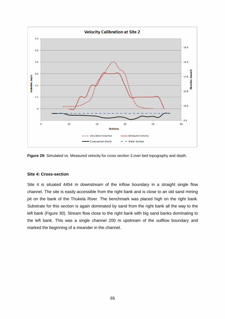
65



Site 4 is situated 4454 m downstream of the inflow boundary in a straight single flow

channel. The site is easily accessible from the right bank and is close to an old sand mining

pit on the bank of the Thukela River. The benchmark was placed high on the right bank.

Substrate for this section is again dominated by sand from the right bank all the way to the

left bank (Figure 30). Stream flow close to the right bank with big sand banks dominating to

the left bank. This was a single channel 200 m upstream of the outflow boundary and

marked the beginning of a meander in the channel.

66


downstream.

Cross-section 4 is shallow with depths averaging below 0.3 m but reaches a maximum of

0.69 m (Figure 31) close to the right bank. Velocities ranged between 0.1 up to 1.3 m/s

(Figure 31) due to this shallow section. After the River2D model was calibrated the velocity

values were extracted for each point where velocities were measured with the global flow

meter along the cross-section. At site 4 the model predicted flow velocities of up to 0.3 m/s

higher than those measure close to the right bank, this is due to the sudden depth increase

in the river. The rest of the cross-section has a strong correlation between the measured and

simulated velocities.

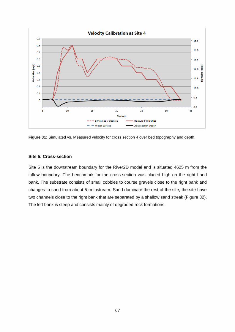
67



Site 5 is the downstream boundary for the River2D model and is situated 4625 m from the

inflow boundary. The benchmark for the cross-section was placed high on the right hand

bank. The substrate consists of small cobbles to course gravels close to the right bank and

changes to sand from about 5 m instream. Sand dominate the rest of the site, the site have

two channels close to the right bank that are separated by a shallow sand streak (Figure 32).

The left bank is steep and consists mainly of degraded rock formations.

68

Figure 32: Cross-section 5 (Sand mining two) with cobbles and silt as substrate A) Total station

setup, B) View across river, C) View upstream, D) View downstream


velocities ranging from an average of 0.2 m/s up to 0.5 m/s (Figure 33). After the River2D

model was calibrated the velocity values were extracted for each point where velocities were

measured with the global flow meter along the cross-section. By comparing the simulated

velocities to those measured (Figure 33) it is possible to see a good correlation between the

two with only slight alterations closer to the river banks. The velocity is fastest in the deeper

channel closest to the right bank and then drops to zero on the sand bank and increases

again in the second channel. The largest difference in velocity between measured and

simulated values for cross-section 5 is 0.1 m/s (Figure 33) and can be explained by the

resistance which the sand bank generates in the middle of the stream.

69


70

4.3. Fish collection and preferences

During the fish collection surveys 29 freshwater and estuarine species of fish were collected

and a total of 1810 specimens. The Species were compared to those in FRAI and it was

decided to use only 19 species (n = 1221) of which all are found in the lower Thukela River

for the fish analyses and preferences (Table 11).

Table 11: Species sampled in the study area and their abundances.

Abbreviation Scientific name Common name Abundance

AAEN Awaous aeneofuscus Freshwater goby 10

ANAT Ambassis natalensis Slender glassy 1

ANG Anguilla spp. Eel 3

CCAR Cyprinus carpio Common carp 1

CGAR Clarias gariepinus Sharptooth catfish 48

CREN Coptodon rendalli Redbreast tilapia 8

EEUT Enteromius eutaenia Orangefin barb 13

EFUS Eleotris fusca Dusky sleeper 16

EPAU Enteromius paludinosus Straightfin barb 13

ETRI Enteromius trimaculatus Threespot barb 42

EVIV Enteromius viviparus Bowstripe barb 3

GCAL Glossogobius callidus River goby 21

LCYL Labeo cylindricus Redeye labeo 3

LMOL Labeo molybdinus Leaden labeo 4

LNAT Labeobarbus natalensis KwaZulu-Natal Yellowfish 299

MCAP Myxus capensis Freshwater mullet 5

OMOS Oreochromis Mossambicus Mozambique tilapia 119

PPHI Pseudocrenilabrus Philander Southern mouth-brooder 45

TSPA Tilapia sparrmanii Banded tilapia 550

The most specimens collected from one species were Tilapia sparrmanii (n = 550) of which

most were juveniles and collected in big shoals with small seine nets. The most abundant

and widely distributed species were KwaZulu-Natal yellowfish Labeobarbus natalensis (n =

299) as shown in Table 11. Eleotris fusca are only found in lowland rivers and need salt

content for juvenile stage and therefore they are considered as an important indicator

species for monitoring natural biodiversity within the ecosystem. The Golden sleeper

Hypseleotris cyprinoides is a near threatened species which has been observed in the study

area and have the same habitat preference as E. fusca and therefore habitat preference of

E. fusca is important not only for a specific species but rather for a group of species with the

same preferences (umbrella species). Figure 34 show some of the different fish species

sampled in the lower Thukela River during surveys.

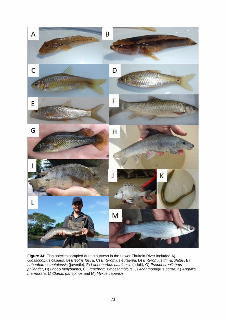
71

Figure 34: Fish species sampled during surveys in the Lower Thukela River included A) Glossogobius callidus, B) Eleotris fusca, C) Enteromius eutaenia, D) Enteromius trimaculatus, E) Labeobarbus natalensis (juvenile), F) Labeobarbus natalensis (adult), G) Pseudocrenilabrus philander, H) Labeo molybdinus, I) Oreochromis mossambicus, J) Acanthopagrus berda, K) Anguilla marmorata, L) Clarias gariepinus and M) Myxus capensis

72

4.3.1. Response of fish community structures to habitat variable conditions

These analyses consist of a high diversity of fish species collected throughout the KwaZulu-

Natal province during different surveys. Due to the adaptiveness of fish data over a range of

rivers and habitats were combined to obtain the most accurate habitat preference for each

species. A multivariate statistical analysis where performed with Canoco in the form of a

Redundancy Analysis (RDA) plot (Figure 35) shows the fish communities and the variance in

the substrate types. It is possible to identify three different groups of species associated with

a change in substrate. The Monte Carlo permutation procedure on the RDA plot shows how

fish community structures change significantly (p < 0.05) with boulders, gravel, sand and silt

(Table 12). Labeobarbus natalensis shows a strong correlation with boulders where P.

philander and O. mossambicus communities are correlated with gravels and sands. Tilapia

sparrmanii has a high correlation with silt and their community structures change significantly

with a change in substrate. The significance of the proportion of mud were marginal (p =

0.174) and cobbles had no significant impacts on fish community structures (Table 12).

These results demonstrate how different fish species have different preferences in substrate

and the importance of maintaining a variety of these substrates within a riverine ecosystem.

Table 12: Statistical change in fish communities of rivers in KZN per effort where substrate types

differ.

Variable Var.N LambdaA P F

Sub. Boulders 8 0.080 0.001 10.540

Sub. Sand 5 0.030 0.003 3.670

Sub. Gravel 6 0.020 0.027 2.740

Sub. Silt 3 0.020 0.042 2.400

Sub. Mud 4 0.010 0.174 1.470

Sub. Cobbles 7 0.000 0.619 0.680

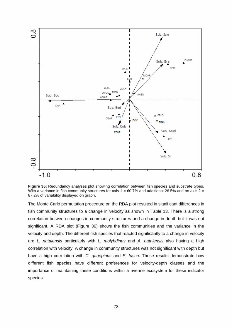
73

Figure 35: Redundancy analyses plot showing correlation between fish species and substrate types. With a variance in fish community structures for axis 1 = 60.7% and additional 26.5% and on axis 2 = 87.2% of variability displayed on graph.

The Monte Carlo permutation procedure on the RDA plot resulted in significant differences in

fish community structures to a change in velocity as shown in Table 13. There is a strong

correlation between changes in community structures and a change in depth but it was not

significant. A RDA plot (Figure 36) shows the fish communities and the variance in the

velocity and depth. The different fish species that reacted significantly to a change in velocity

are L. natalensis particularly with L. molybdinus and A. natalensis also having a high

correlation with velocity. A change in community structures was not significant with depth but

have a high correlation with C. gariepinus and E. fusca. These results demonstrate how

different fish species have different preferences for velocity-depth classes and the

importance of maintaining these conditions within a riverine ecosystem for these indicator

species.

74

Table 13: Statistical change in fish communities of rivers in KZN per effort where velocity-depth

classes differ

Variable P F

Velocity 0.001 7.99

Depth 0.058 2.07

Most species did not show any correlation with depth and velocities and therefore they were

not considered as indicator species to determine the EFR (Figure 36).

Figure 36: Redundancy analyses plot showing correlation between fish species and velocity-depth classes. With a variance in fish community structures for axis 1 = 84.5% and additional 15.5% and on axis 2 = 100% of variability displayed on graph.

75

4.3.2. Habitat preference assessment

Velocity and depth were collected for each effort and 19 different fish species caught during

surveys in KZN. Species observed in the study area make use of a wide variety of flows

(Figure 37). Species like L. natalensis and L. molybdinus have a preference for flow

velocities ranging from 0.25 m/s to 0.63 m/s and some were found in velocities as high as

0.86 m/s. Sharptooth catfish (C. gariepinus) have the widest preference from no flow up to

0.51 m/s with some specimens found in 0.74 m/s, these species make use of a range of

different habitats and flow conditions which suggests that these fish are adapted and

relatively tolerant to habitat change. Other species that had a preference for low velocities

were A. aeneofuscus, E. fusca and G. callidus ranging between 0 m/s (pools) to 0.34 m/s

with A. aeneofuscus and E. fusca rarely found in velocities higher that 0.5 m/s. The

confidence of A. natalensis and C. carpio were too low to describe preference for these

species due to low abundances. The Enteromius species E. eutaenia, E. paludinosus and E.

trimaculatus as well as other species including O. mossambicus, C. rendalli and T.

sparrmanii had very low preferences for velocities and was found between 0 m/s and 0.27

m/s. The only barb species that had a preference for faster velocities were E. viviparus and

was found between 0.22 m/s and 0.56 m/s.

Figure 37: Box (25th to 75

th percentile) and whisker (max and min value) for water velocity habitats

associated with species observations in KZN.

0.0

0.1

0.2

0.3

0.4

0.5

0.6

0.7

0.8

0.9

1.0

AA

EN

(n=

10)

AN

AT

(n=

1)

AN

G (

n=

3)

EE

UT

(n=

30)

LN

AT

(n=

299)

EP

AU

(n=

13)

ET

RI (n

=42)

EV

IV (

n=

3)

CC

AR

(n=

1)

CG

AR

(n=

48

)

EF

US

(n=

16)

GC

AL

(n=

21)

LC

YL (

n=

3)

LM

OL

(n=

4)

MC

AP

(n=

5)

OM

OS

(n=

119)

PP

HI (n

=45

)

CR

EN

(n=

8)

TS

PA

(n=

550)

Species

Velocity preferences of Species

Ve

loc

ity m

/s

76

Sampling deeper than 1.2 m is difficult with the techniques used and due to available depth

during surveyed times therefore it is difficult to predict the higher percentile for preference

depth and it was assumed that preference will increase with depth. The maximum depth will

not determine or have an effect on the EFR and the minimum depth requirement only

indicates that the fish are able to survive and not thrive in these habitats. Therefore the

median value for depth was used to create a depth preference file (Figure 38). No fish were

caught in areas shallower than 150 mm with most species caught in a depth of more than

300 mm. Labeobarbus natalensis and L. molybdinus preferred depths between 300 mm and

440 mm, where C. gariepinus had a preferred depth of approximately 500 mm. A.

aeneofuscus and Eleotris fusca showed preference for deep water >550 mm. All species

were collected in an average depth of 400 mm which is considered to represent suitable

cover for fish.

Figure 38: Box (25th to 75

th %tile) and whisker (max and min value) for water depth habitats

associated with species observations.

Two indicator species were selected one representing high velocities and deep habitats and

another representing slow velocities and deep habitats typical of lowland rivers.

Labeobarbus natalensis were used as an indicator species to characterise fast-deep habitats

that cover a range of preferred habitats by other species as well and therefore can be

considered an important criteria for the lowland river. Upstream of the study area steep rocks

are present, this acts as a natural boundary to fish which makes it impossible for

communities in the lower Thukela River to migrate upstream for feeding and breeding during

low flows, fish can only migrate upstream under severe high flows and therefore it is

important to protect the Yellowfish communities in the lower Thukela River. E. fusca was

0

200

400

600

800

1000

1200

AA

EN

(n=

10)

AN

AT

(n=

1)

AN

G (

n=

3)

EE

UT

(n=

30)

LN

AT

(n=

299)

EP

AU

(n=

13)

ET

RI (n

=42)

EV

IV (

n=

3)

CC

AR

(n=

1)

CG

AR

(n=

48

)

EF

US

(n=

16)

GC

AL

(n=

21)

LC

YL (

n=

3)

LM

OL

(n=

4)

MC

AP

(n=

5)

OM

OS

(n=

119)

PP

HI (n

=45

)

CR

EN

(n=

8)

TS

PA

(n=

550)

Species

Depth preferences of Species

De

pth

(m

m)

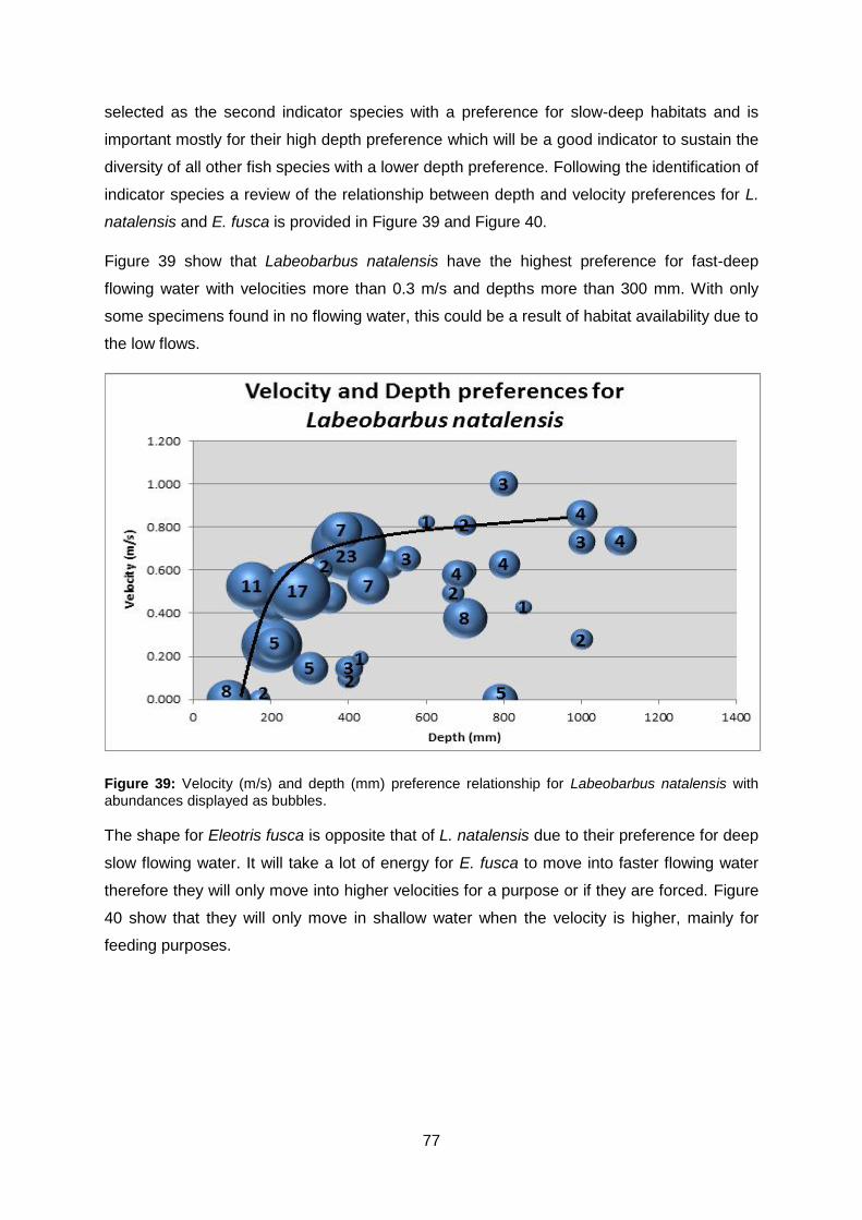
77

selected as the second indicator species with a preference for slow-deep habitats and is

important mostly for their high depth preference which will be a good indicator to sustain the

diversity of all other fish species with a lower depth preference. Following the identification of

indicator species a review of the relationship between depth and velocity preferences for L.

natalensis and E. fusca is provided in Figure 39 and Figure 40.

Figure 39 show that Labeobarbus natalensis have the highest preference for fast-deep

flowing water with velocities more than 0.3 m/s and depths more than 300 mm. With only

some specimens found in no flowing water, this could be a result of habitat availability due to

the low flows.

Figure 39: Velocity (m/s) and depth (mm) preference relationship for Labeobarbus natalensis with

abundances displayed as bubbles.

The shape for Eleotris fusca is opposite that of L. natalensis due to their preference for deep

slow flowing water. It will take a lot of energy for E. fusca to move into faster flowing water

therefore they will only move into higher velocities for a purpose or if they are forced. Figure

40 show that they will only move in shallow water when the velocity is higher, mainly for

feeding purposes.

78

Figure 40: Velocity (m/s) and depth (mm) preference relationship for Eleotris fusca with abundances

displayed as bubbles.

Substrate preferences of species were evaluated and results showed that most species

were observed in a wide variety of different substrates but preference to one or more

substrate types dominated (Figure 41). Species like L. natalensis and L. molybdinus have a

high preference for boulders although they are found in sand, bedrock, cobbles and gravel.

Most of the species have a high preference for boulders including C. gariepinus, Awaous

aeneofuscus, Enteromius eutaenia, Enteromius trimaculatus, and Enteromius viviparus.

Species with a higher preference for sand included Glossogobius callidus and Myxus

capensis. Eleotris fusca are found in many substrates with silt dominating and are followed

by sand, boulders and solid bedrock.

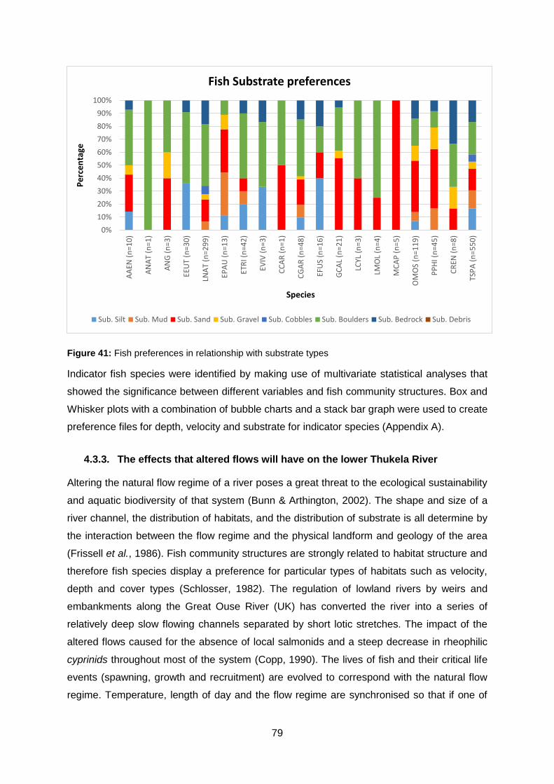
79

Figure 41: Fish preferences in relationship with substrate types

Indicator fish species were identified by making use of multivariate statistical analyses that

showed the significance between different variables and fish community structures. Box and

Whisker plots with a combination of bubble charts and a stack bar graph were used to create

preference files for depth, velocity and substrate for indicator species (Appendix A).

4.3.3. The effects that altered flows will have on the lower Thukela River

Altering the natural flow regime of a river poses a great threat to the ecological sustainability

and aquatic biodiversity of that system (Bunn & Arthington, 2002). The shape and size of a

river channel, the distribution of habitats, and the distribution of substrate is all determine by

the interaction between the flow regime and the physical landform and geology of the area

(Frissell et al., 1986). Fish community structures are strongly related to habitat structure and

therefore fish species display a preference for particular types of habitats such as velocity,

depth and cover types (Schlosser, 1982). The regulation of lowland rivers by weirs and

embankments along the Great Ouse River (UK) has converted the river into a series of

relatively deep slow flowing channels separated by short lotic stretches. The impact of the

altered flows caused for the absence of local salmonids and a steep decrease in rheophilic

cyprinids throughout most of the system (Copp, 1990). The lives of fish and their critical life

events (spawning, growth and recruitment) are evolved to correspond with the natural flow

regime. Temperature, length of day and the flow regime are synchronised so that if one of

0%

10%

20%

30%

40%

50%

60%

70%

80%

90%

100%

AA

EN (

n=1

0)

AN

AT

(n=1

)

AN

G (

n=

3)

EEU

T (n

=30

)

LNA

T (n

=29

9)

EPA

U (

n=1

3)

ETR

I (n

=42

)

EVIV

(n

=3)

CC

AR

(n

=1

)

CG

AR

(n

=48

)

EFU

S (n

=16

)

GC

AL

(n=

21

)

LCYL

(n

=3)

LMO

L (n

=4)

MC

AP

(n

=5

)

OM

OS

(n=1

19

)

PP

HI (

n=

45

)

CR

EN (

n=8

)

TSP

A (

n=

55

0)

Pe

rce

nta

ge

Species

Fish Substrate preferences

Sub. Silt Sub. Mud Sub. Sand Sub. Gravel Sub. Cobbles Sub. Boulders Sub. Bedrock Sub. Debris

80

these natural factors are not in harmony it will cause a disturbance in fish behaviour (Copp,

1990; Sparks, 1995). Spawning of certain species are triggered with a rise in flow as for

Colorado River squawfish (Ptychocheilus lucius) in the Yampa River and Clanwilliam

yellowfish (Labeobarbus capensis) in the Western Cape (King et al., 1998).

Construction of barriers even small in-stream barriers, such as v-notch gauging weirs can

lead to isolation of populations and local extinction for e.g. the Western minnows (Galaxias

occidentalis) in south-western Australian forest streams (Pusey et al., 1989). Invading fish

species are more successful in rivers that are permanently altered by humans. The

regulation or reduction in flows will favour species that are adapted to the modified flow

regime like carp (Cyprinus carpio) and mosquitofish (Gambusia affinis) (Edwards, 1978;

Faragher & Harris, 1994; Walker et al., 1995). Flow alteration is a serious threat in the lower

Thukela River with the new weir that has been build upstream of the study area, water

extraction of SAPPI and other water use activities e.g. agriculture and irrigation. The

following biotic responses are a direct result of altered flows and some of them are already

visible in the lower Thukela River:

Loss of fishes adapted to turbid river habitats.

Delayed spawning in fish.

Loss of cues for fish spawning and migration.

Favourable populations of exotic fish species (carp, mosquitofish).

Loss of migratory fish species.

Reduced spawning areas and/or recruitment success of lowland river fish.

4.4. Ecological flow requirements

Ecological flow requirements are highly variable depending on the purpose of the study as

well as the methods used. In this study both the historic method and the habitat method

were done and compared. The historic data were processed by making use of the ABF

method as well as the Tennants (1976) method. The ABF method (Figure 42) predicts the

median flow and the base flow which is 70% of the median monthly flow. Data were

collected from the Department of Water and Sanitation website from 1963 to 2016. The data

were collected in daily average flows and converted into average monthly flows for each

year. The data were then edited into percentiles of flow including the 10th, 30th, 50th and 70th

percentile showing natural flows which exceeded for that specific percentages of the time

(Table 14).

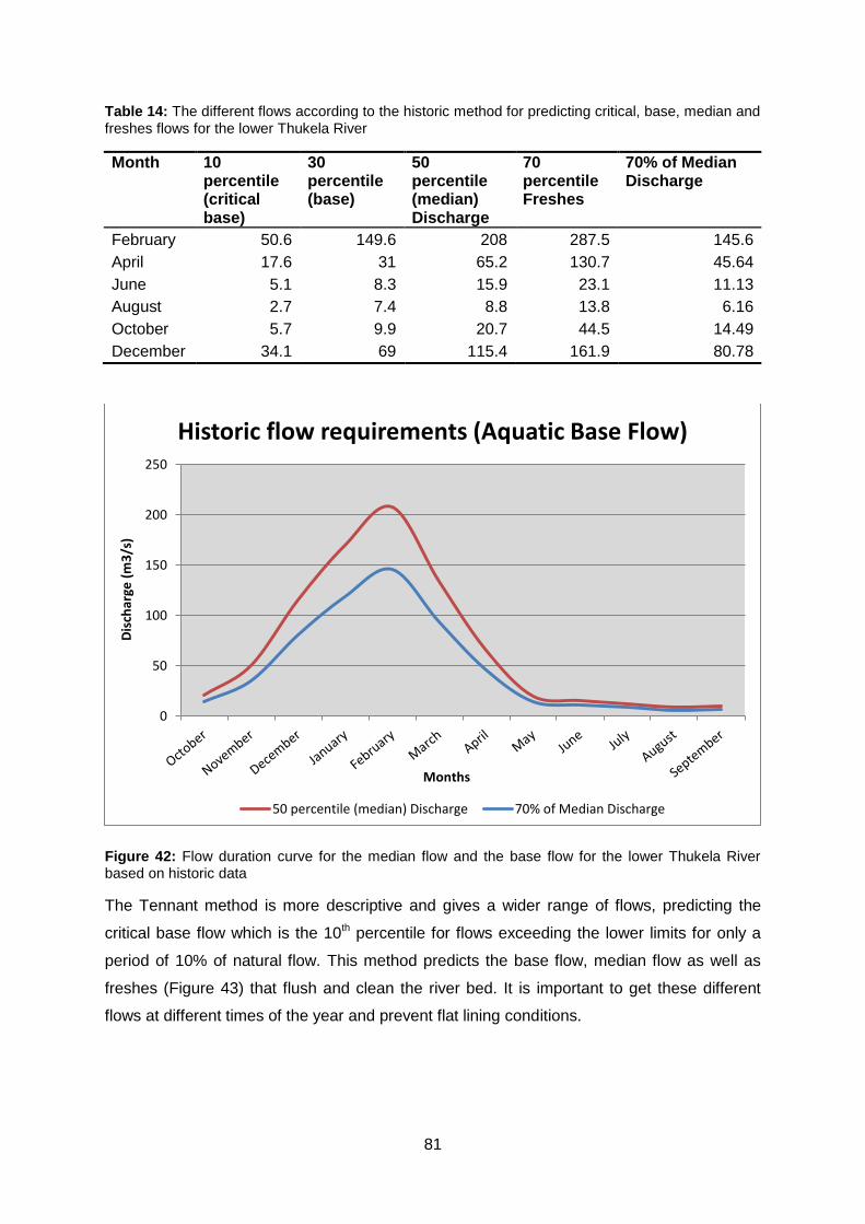
81

Table 14: The different flows according to the historic method for predicting critical, base, median and

freshes flows for the lower Thukela River

Month 10 percentile (critical base)

30 percentile (base)

50 percentile (median) Discharge

70 percentile Freshes

70% of Median Discharge

February 50.6 149.6 208 287.5 145.6

April 17.6 31 65.2 130.7 45.64

June 5.1 8.3 15.9 23.1 11.13

August 2.7 7.4 8.8 13.8 6.16

October 5.7 9.9 20.7 44.5 14.49

December 34.1 69 115.4 161.9 80.78

Figure 42: Flow duration curve for the median flow and the base flow for the lower Thukela River based on historic data

The Tennant method is more descriptive and gives a wider range of flows, predicting the

critical base flow which is the 10th percentile for flows exceeding the lower limits for only a

period of 10% of natural flow. This method predicts the base flow, median flow as well as

freshes (Figure 43) that flush and clean the river bed. It is important to get these different

flows at different times of the year and prevent flat lining conditions.

0

50

100

150

200

250

Dis

char

ge (

m3

/s)

Months

Historic flow requirements (Aquatic Base Flow)

50 percentile (median) Discharge 70% of Median Discharge

82

Figure 43: Flows for different months using the Tennants (1976) method to predict critical base, base,

median and freshes flows for the lower Thukela River

The critical base is determined by the 10th percentile of the month with the lowest average

monthly flow which is 2.7 m3/s for the lower Thukela River and occurs in the month of

August. According to Jowett (1997) velocity and depth are degraded at critical base flow and

it would only provide short-term survival for aquatic life, fish will not be able to breed or feed

in this habitat and will use all their energy for survival. They are under greatest stress and

the aquatic ecosystem cannot be exposed to these conditions for extended periods of time

and therefore it is important to avoid these conditions at all costs, sometimes impossible due

to droughts. The role of temperature changes in drought conditions should be considered as

it can lead to oxygen depletion and cause physiological stress which lower spawning ability

and have negative impacts on fish populations.

Base flow at 30% of the average flow as predicted by the Tennants method is 7.4 m3/s

during low flow months and is considered to provide satisfactory stream width, depth and

velocity for a baseflow regime (Jowett, 1997). The base flow for wet periods (summer) is

149.6 m3/s and can be described as the minimum flow requirements for fish populations

during high flows to maintain population structures. This flow will allow fish to migrate

upstream for spawning and feeding and is of critical importance.

0

50

100

150

200

250

300

350

Dis

char

ge (

m3/s

)

Months

Historic flow requirements (Tennants method)

10 percentile (critical base) 30 percentile (base)

50 percentile (median) Discharge 70 percentileFreshes

83

By using the historic method in calculating environmental flow requirements for the Thukela

River fish populations will only be maintained in the current state. For the lower Thukela

River it is important to set a flow requirement that is higher than the current natural base

flow, due to the decrease in available habitat and fish preferences that are influenced by

human activities upstream of the study area. Labeobarbus natalensis highest substrate

preference is boulders and with the current state of sand in the lower Thukela River boulders

will be completely covered with sand in the near future. This would not have been a problem

if fish could migrate freely upstream, but due to the barrier created by SAPPI for their

extraction fish are unable to migrate over the rocky areas to better spawning habitat except

for times of very high flow and therefore the median natural flow will be a more suitable flow

requirement at 8.8 m3/s in winter and 208 m3/s in summer. The higher flow in winter will

allow better cover and more habitats for different fish species and will have a lower stress

factor on population structures, where the high flow in summer will allow fish species to

migrate upstream to spawn and feed.

A comparison between the ABF method and the Tennant’s (1976) method for base flows

were done in Figure 44. The difference between these two methods for predicting the base

flows are very close with a difference of less than 1.3 m3/s for the dry period in august and

as little as 4 m3/s for wet period.

Figure 44: Aquatic Base Flow method vs. Tennant (1976) method for base flows

Habitat data were collected during field surveys by making use of different techniques, the

bathymetric data for the Thukela River were done with a total station and a level logger while

0

20

40

60

80

100

120

140

160

Dis

char

ge (

m3/s

)

Months

Aquatic Base Flow vs. Tennant's method

70% of Median Discharge 30 percentile (base)

84

topographic data were edited and processed in ArcGIS. River2D was used to calculate the

WUA on the same concept used by PHABSIM. River2D is a 2-dimensional model which

gives a good spatial coverage of the study area. The study area is 4.6 km long and the river

bed is on average more than 100 meters wide. The unit for WUA is m2/m and represent the

available habitat as an index of habitat rather than an area. The WUA have to be calculated

for each indicator species within River2D by making use of the same index file but different

preference files. Preference files should be loaded for each individual species and for this

study two species were used, L. natalensis with a high preference for deep fast flowing water

and E. fusca which had a higher preference for deep slow flowing water. The result for each

species was calculated in River2D with different flows (Table 15).

Table 15: WUA in the lower Thukela River for LNAT and EFUS with an increase in discharge

Discharge m3/s

LNAT WUA m2/m EFUS m2/m Total units

2.7 6590.7 0.94 60222.8 8.58 701546.7

4.3 9449.5 1.35 63429.3 9.04 701546.7

8.8 14010.5 2.00 69353.9 9.89 701546.7

13.8 20887.4 2.98 70077.8 9.99 701546.7

21.1 25267.3 3.60 71819.8 10.24 701546.7

50.6 27947.9 3.98 74604.7 10.63 701546.7

208 16929.5 2.41 90324.7 12.88 701546.7

509.5 16055.1 2.29 100866 14.38 701546.7

The rate of habitat change varies with flow and therefore habitat modelling results of WUA

against discharge can be plotted on a graph for each species (Figure 45 and Figure 46). The

rate of change is used as the basis for setting a minimum flow for each indicator species.

The point of greatest change in the rate (the breakpoint) is used as the minimum flow

requirement for the lower Thukela River. The total unit of available WUA is not that important

rather the point of greatest change, this is because the graphs shape will remain the same

even though the value will increase or decrease at different sites. The minimum flow

requirement for L. natalensis is 15 m3/s, this does not mean that the species will require this

minimum flow for survival but rather to thrive in an environment with favourable habitat.

85

Figure 45: Selection of minimum flow for L. natalensis at the breakpoint: point where habitat begins to

degrade sharply with a decrease in flow

The minimum flow requirements for E. fusca is 8 m3/s (Figure 46), they will be able to

survive in lower flow conditions but to reach their full potential and to benefit their ecological

state these minimum requirements needs to be maintained.

Figure 46: Selection of minimum flow for E. fusca at the breakpoint: point where habitat begins to

degrade sharply with a decrease in flow

86

According to a reserve determination study of the Department of Water Affairs and Forestry

done in 2003 the minimum flow requirements for the lower Thukela River is 7.7 m3/s (DWAF,

2004). This is relatively low and was calculated based on historic flow data only and not in

combination with other methods. A higher reserve for environmental flow requirements are

suggested by the results of this study.

Habitat methods are quantitative and incorporate biological principles and therefore have

been considered more reliable than assessments made by means of other methods (Annear

& Conder, 1984). In this study two separate species were used as indicator species L.

natalensis and E. fusca. Labeobarbus natalensis were used to determine the upper limit of

ecological flow requirements as it is a rheophillic species with preferences for fast-deep

flows (Pander et al., 2013) and E. fusca as a non-rheophillic species with higher preferences

for slow-deep flowing habitats (Linnansaari & Cunjak, 2007). It is important to use different

species with different preferences and importance to the ecological state of the Thukela

River to determine flows that will optimise the ecological state of the river. Labeobarbus

natalensis is more important on a socio-economic scale for recreational and subsistence

fisheries where E. fusca is more important from a conservation perspective and represents

the flow requirements that needs to be maintained to protect species like H. cyprinoides. The

flow requirements as determined by the habitat method for L. natalensis are 15 m3/s and for

E. fusca is 8 m3/s. It is difficult to determine environmental flow requirements for a specific

species and therefore it was assumed that higher flow requirements would maintain and

benefit species with lower requirements (Jowett et al., 2008) and to enhance the ecological

state of the Thukela River, flows that would benefit all species needs to be maintained as

closely as possible. The whole life cycle of different fish species should be considered and

sustainable flows are required for fry to complete its growth in inundated areas for optimal

food, habitat and temperature conditions.

It is assumed that minimum flows set for rheophillic species like L. natalensis will be

adequate to maintain native fish populations in the lower Thukela River (Jowett et al., 2008).

The reason for this is due to their large size and feeding habits of the natal Yellowfish giving

them a higher preference for fast-deep flowing water than that of most native species.

Smaller native fish species have preferences for slow-deep flowing water and are most

abundant at the margins of the Thukela River with habitat availability at its maximum with

low flows. The margins of the river will still provide suitable habitats for these species even

with an increase in flow velocity and depth (Jowett et al., 2008). Nevertheless it is still

inappropriate to set flows with these high requirements as it would be impossible for the

natural flow regime to sustain these requirements, flow requirements if determined only by

maximum habitat for rheophillic species is higher than median low flows. The conservation

87

status of some species like the H. cyprinoides warrants special attention (Vrdoljak & Hart,

2007). This specific species could not be sampled during the time of the study and therefore

E. fusca a species with the same preferences were also considered for minimum flow

requirements. These species occur only in lowland rivers with estuarine conditions and are

just as important to keep the aquatic diversity in the ecosystem.

There are many different fish species and life stages in the Thukela River at any given time

and thus cause for a conflict in flow requirements. Certain species juveniles may be found in

low velocities and prefer an increase in velocities as their size and ability to swim increases.

In rivers with small habitat variability the different species will benefit with different flows,

where some species may find a reduction in depth and velocity as beneficial other species

habitat will decrease (Jowett, 1997). Compromises like adjusting the flow requirements to

different seasonal life stages are possible by increasing the flow requirements for spawning,

rearing and adult habitats. Another method is to adjust the flow requirements based on

seasons, the biological habitat requirements for fish species may be less in winter as food

requirements and their metabolic rate decreases with a decrease in temperature (Caissie &

El-Jabi, 1995). The flow requirements of individual species vary and therefore it is important

to find a neutral flow requirement that will suit all species habitat requirements or by defining

flow requirements for aquatic communities.

Instream habitat will decrease as flows fall below the optimum value and therefore there is

no clear point at which instream habitat can be identified as good or bad although the rate of

decrease may vary with flows (Jowett et al., 2008). The rate of change is therefore often

used as the basis for describing a minimum flow requirement by selecting the point of

greatest change (the breakpoint). This concept is based on the principle that higher flows will

lessen optimum habitat conditions although the diminishing effect of a greater than optimum

flow is less than that of a lower than optimum flow (Jowett et al., 2008). Habitat loss

associated with higher flows can be balanced due to the increase of food availability, cover

or the ability to migrate and spawn. In wide rivers like the Thukela River habitats like

shallow-slow flowing water will always be available near river banks as the water level rises

and bank flow will only be reached in times of flood.

To estimate the minimum flow requirements in a river a habitat suitability curve is required,

this is obtained by modelling instream habitat for a range of flows for each indicator species.

In this study River2D was used to calculate the habitat suitability for Labeobarbus natalensis

(Figure 47) and Eleotris fusca (Figure 48) . The valuation of an appropriate minimum flow for

a river is complex and there are no computers that can assist with this step. River2D make

use of the PHABSIM concept WUA, and can be seen as an index of usable habitat rather

88

than a physical area although WUA has units of m2/m (Paxton, 2008). When binary habitat

criteria is used as for this study (0 is unsuitable and 1 is most suitable) the WUA can be used

as a physical area (m2). The PHABSIM concept is criticised due to the posibility that a large

area of sub-optimal habitat or a small area of optimum habitat will both result in a high WUA.

By examining the habitat suitability index (HSI) (habitat index score at each node averaged

over the reach) and how it changes with flow can be a solution to this problem (Jowett et al.,

2008). It is equal to WUA (m2/m) divided by the average water surface width of the river, by

interpretation of these results it is possible to identify flows with most suitable habitats.

Substrate size can be taken into consideration when evaluating habitat suitability where

particle size is determined by velocities and depths at channel forming flows. Habitat

analyses to determining base flows is normally lower than that of channel forming flows and

it can be assumed that substrate size will not change. In the lower Thukela River the

substrate consists mainly of coarse sand particles causing the river bed to be very dynamic

and channel forming flows to be very low. It was assumed that even though the channel

shape might change the habitats (velocity-depth) in relation to stretch area will stay the same

and therefore the 2D model is relevant. It was possible to calculate flows and habitat

availability over substrate and to predict flows that would provide the most suitable habitat

for different species at different flows. Substrate composition and distribution does not

influence the shape of habitat-flow relationships and this was tested by calculating the

relationship with and without substrate suitability, giving a higher total WUA without substrate

suitability but the shape of the curve remained the same and therefore the flow

requirements.

The biological interpretation of the results is the most uncertain and difficult part of an

instream habitat analysis. The key elements are to calculate WUA with habitat suitability and

the linkage between available habitat and the abundance of aquatic populations (Paxton,

2008). No given aquatic species can be maintained in a river or stream without some form of

suitable habitat and therefore the importance of habitat analyses cannot be undermined. The

relationship between species abundance and habitat availability is not directly linked or flow

related and there are many other factors that can influence species abundance like food,

migration patterns and spawning periods (Jowett et al., 2008). Therefore habitat suitability

would not indicate the abundance of any given species for any given time but rather set the

lower limited of possible population size of a species in an area.

The only way to ensure relief for fish under times of high stress is by means of freshes, this

is a natural high flow for short periods of time (flash flood) and is the limit at which 80% of

bed material covered by water gets mobile (King et al., 1998). The timing and frequency of

89

freshes is important for the sustainability of fish populations and it is recommended that

freshes takes place as many as 2 times during low flow periods (May – September) and 6

times during high flow periods (October - April). Freshes flow can be calculated by using the

historic method with the 70th percentile which is 13.8 m3/s for low flow and 287.5 m3/s for

high flows (King et al., 2000). These flows will allow periodical stress relief in terms of some

spawning and feeding for fish in winter months and more specifically in summer month with

fish migration to spawning grounds and new habitat availability at overbanks for feeding.

Habitat suitability in the form of WUA for different flows is attached in Appendix B.

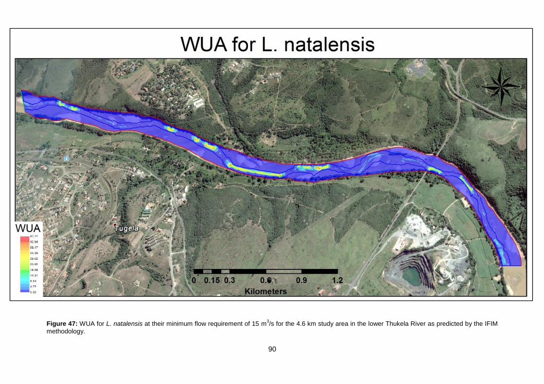
90

Figure 47: WUA for L. natalensis at their minimum flow requirement of 15 m3/s for the 4.6 km study area in the lower Thukela River as predicted by the IFIM

methodology.

91

Figure 48: WUA for E. fusca at their minimum flow requirement of 8 m3/s for the 4.6 km study area in the lower Thukela River as predicted by the IFIM

methodology.

92

5. Conclusion

Bathymetric data collected with a Total Station and an Aquameter were combined with

topographic data in ArcGIS to create a Digital Elevation Model. By using HECGeo-RAS to

generate additional bathymetric data in combination with the DEM created in GIS, it was

possible to delineate cross-sections, flow boundaries, river banks and flood plains for the

lower Thukela River in areas which was inaccessible to reach. Data created were exported

from HECGeo-RAS to HEC-RAS and bathymetric data were refined within the program to

ensure accurate modelling. The model was calibrated for steady flow analysis at a discharge

of 4.3 m3/s as measured on the survey of April 2016 and a satisfactory correlation between

measured and simulated water elevations were obtained. In addition another 22 different

flows were simulated for the lower Thukela River ranging from 1 m3/s to 4000 m3/s to

generate a stage-discharge curve. This played an important part in the study to generate

water levels for different discharges as there were only two points from surveyed data

available.

Topographic and bathymetric data used in GIS and HEC-RAS were used to create a bed

profile for River2D, a 2-Dimensional hydraulic model. The model data were triangulated and

exported as a mesh file and could then be refined in the MESH section of River2D where

boundary conditions are set before final exportation to River2D for flow simulations. Water

elevation data generated by HEC-RAS were used as the downstream boundary for River2D.

After model calibration for steady state analysis measured and simulated velocities, surface

water elevation and cross-section depth were compared and showed a good correlation.

To determine the habitat requirements and preferences, 19 freshwater and estuarine fish

species (n = 1221) relevant to the lower Thukela River were used in the analyses.

Multivariate statistical analyses were performed in the form of a Redundancy Analysis plot to

determine the groups of species associated with a change in substrate, velocity and depth.

The Monte Carlo permutation procedure on the RDA plot indicated that fish community

structures change significantly with a change in substrate. Velocity had a significant effect on

fish community structures while depth showed a strong correlation for some species but not

significant.

Habitat preference assessments were done for all fish species in the form of velocity, depth

and substrate. Box and Whisker plots were used to generate preferences for velocity and

depth and a stack bar graph was used to identify preferred substrate types for different

species. KwaZulu-Natal yellowfish (Labeobarbus natalensis) was the most abundant and

widely distributed species and showed a strong correlation between substrate and velocities,

93

and therefore was used as an indicator species for fast-deep habitat conditions. The Dusky

sleeper (Eleotris fusca) was identified as the other indicator species as it is endemic to

lowland rivers and its velocity and flow preferences can act as a double for the Golden

Sleeper (Hypseleotris cyprinoides) that is near threatened. The preference values for

indicator species were converted to binary units with 0 being the least preferred habitat and

1 the most preferred habitat to get unit area in square meters. River2D make use of the

PHABSIM concept to calculate WUA (m2/m) by combining habitat suitability (substrate) with

velocity and depth preferences.

Flow alteration is a serious threat in the lower Thukela River due to anthropogenic changes

upstream that disturb the natural flow-regime. The reduction in flow will have many negative

effects on the endemic fish populations including the loss of rheophillic species, and delayed

or loss of spawning and migration of different species. The reductions in flows will also

benefit exotic species like carp and mosquitofish that are already present in the lower

Thukela River. These effects pose a great threat to the existence of the natural aquatic

biodiversity and therefore it is important to determine environmental flows that will improve

the current ecological state of the river.

Different historic methods have been used as well as a habitat method to determine the

environmental flow for the lower Thukela River. The historic methods that were used and

compared are the Tennants method (1976) and the Aquatic Base Flow method. The flow

requirements determined through the historic methods were both lower than that of the

habitat method used in River2D. By using the historic methods it is assumed that by

maintaining the natural flow regime the ecological state of the river will be maintained, but

does not make provision for anthropogenic changes within the system. The lower Thukela

River have been altered by the bulk water supply scheme and the abstraction at the SAPPI

mill and therefore the habitat method to determine environmental flow requirements are

more relevant to the study area. The habitat method provides a flow requirement for each

individual species and their life stages and therefore conflict between flow requirements do

exist. It is an accepted practice to use species with higher flow requirements, rheophillic

species like L. natalensis, to determine the environmental flow requirement as this will

maintain and benefit all species with lower flow requirements. The margins of the river

channel will still provide sufficient habitat suitability for smaller native fish species. The

environmental flow requirement determined by this study is higher than the flow requirement

determined by the DWAF (2004) and therefore suggests that the environmental flow

requirements for the lower Thukela River is increased to avoid the negative impact

associated with a reduction in flow.

94

Environmental flows describe the quantity, quality and timing of water flows required to

sustain freshwater ecosystems. The flow regime consist of different components like low

flows, freshes, channel maintenance and floods and even though the importance of these

flows are known, the degree to which the frequency and durations of these flows affect the

biota are unknown and there are no clear method for assigning values to these components

other than mimicking natural flows. Low flow requirements can be considered as the most

important flow requirement for a river and with flows lower than the minimum requirements

aquatic life will decrease drastically. By only maintaining base flow conditions for a river

ecosystem the ecological state of the river may stay the same or degrade and therefore it is

important to have variable flows..

No model exists that can be globalised and for that reason it is important not to use habitat

analysis as a decision making process itself but rather as a tool to assist in the process of

establishing flow requirements. This is achieved when the goals for flow requirements are

clear and target objectives for the effect of flow on the ecological state are identified, to

maintain or improve the ecological state of a river.

https://en.wikipedia.org/wiki/Freshwater_ecosystem

https://en.wikipedia.org/wiki/Ecosystem

95

6. Recommendations

By doing this study a few shortcomings were identified both in data collection and that of

natural conditions. The greatest limitation was the collection of bathymetric data due to

inaccessibility and the dangers of crocodiles in the river. The use of a total station provided

limited data and for future studies sampling bathymetric data with an Acoustic Doppler

Current Profiler (ADCP) over larger areas is recommended. This will allow higher detail of

river bed profiles. It is recommended that if possible LIDAR data should be used for the

topography data rather than 5 m contours to improve accuracy of high flow predictions that

will flood river banks. Due to the dynamic nature of the lower Thukela River the model will

need to be updated for new studies to ensure accurate distribution of habitat classes as they

will change after high flows and floods. The fish preference file can be used again and

additional fish data collected can be added to existing files to increase reliability.

Additional studies that are required to determine true instream requirements and their timing

for the lower Thukela River includes the stage/flow requirement for fish to migrate actively

over the rocky barrier of SAPPI’s extraction point. The impact altered flows will have on the

chemical properties of the lower Thukela River and to what extend the concentration of

harmful chemicals will increase must be considered in combination with the physical

properties for a better understanding in timing and extend of freshes and flood requirements.

An increase in sediment due to human activities upstream will decrease habitat suitability

downstream and therefore studies incorporating sediment transport will proof of great value

for decision making.

Temperature plays an important role in the distribution of different fish species and should be

considered as a parameter in future studies.

It is important to conduct a groundwater-surface water interaction study on the lower Thukela

River to determine the magnitude of groundwater contribution to the baseflow conditions.

Groundwater-surface water interaction will have a significant contribution to available

ecological habitat within a river and therefore groundwater-dependant ecosystems needs

more research in terms of understanding the contribution and linkages between groundwater

and surface water. This will require intrusive work along the river banks.

96

7. References

Allanson, B.R., Hart, R., O'keeffe, J. & Robarts, R. 2012. Inland waters of Southern

Africa: an ecological perspective. Vol. 64: Springer Science & Business Media.

Annear, T.C. & Conder, A.L. 1984. Relative bias of several fisheries instream flow

methods. North American journal of fisheries management, 4(4B):531-539.

Arthington, A.H. & Zalucki, J.M. 1998. Comparative evaluation of environmental

flow assessment techniques: review of methods.

Beck, J. & Basson, G.R. 2003. The hydraulics of the impacts of dam development

on the river morphology: Water Research Commission.

BKS. Dwaf. 2001. Thukela water project feasibility study – main feasibility report.

Pretoria. (V000-00-9700).

Brown, C., Eeekhout, S. & King, J. 1996. National Biomonitoring Programme for

Riverine Ecosystems: Proceedings of Spatial Framework Workshop, 23-24 January

1996, the Breakwater Lodge, Victoria and Alfred Waterfront, Cape Town:

Department of Water Affairs and Forestry.

Brown, C., Ewart-Smith, J., Conrad, J., Rossouw, N., Dollar, E. & Nicolson, C. 2007.

The development of the water resource classification system (WRCS). Volume 2.

Ecological, hydrological and water quality guidelines for the 7-step classification

procedure.

Brunner, G.W. 2001. HEC-RAS River Analysis System: User's Manual: US Army

Corps of Engineers, Institute for Water Resources, Hydrologic Engineering Center.

Bunn, S.E. & Arthington, A.H. 2002. Basic principles and ecological consequences

of altered flow regimes for aquatic biodiversity. Environmental management,

30(4):492-507.

Caissie, D. & El-Jabi, N. 1995. Comparison and regionalization of hydrologically

based instream flow techniques in Atlantic Canada. Canadian Journal of Civil

Engineering, 22(2):235-246.

97

Capra, H., Breil, P. & Souchon, Y. 1995. A new tool to interpret magnitude and

duration of fish habitat variations. Regulated Rivers: Research & Management,

10(2‐4):281-289.

Copp, G.H. 1990. Effect of regulation on 0+ fish recruitment in the Great Ouse, a

lowland river. Regulated Rivers: Research & Management, 5(3):251-263.

Crowe, A., Hayes, J., Stark, J., Strickland, R., Hewitt, T. & Kemp, C. 2004. The

current state of the Maitai River–a review of existing information. Prepared for

Cawthron Institute.

De Winnaar, G. & Jewitt, G. 2010. Ecohydrological implications of runoff harvesting

in the headwaters of the Thukela River basin, South Africa. Physics and Chemistry

of the Earth, Parts A/B/C, 35(13):634-642.

De Winnaar, G., Jewitt, G. & Horan, M. 2007. A GIS-based approach for identifying

potential runoff harvesting sites in the Thukela River basin, South Africa. Physics

and Chemistry of the Earth, Parts A/B/C, 32(15):1058-1067.

Dudgeon, D., Arthington, A.H., Gessner, M.O., Kawabata, Z.-I., Knowler, D.J.,

Lévêque, C., et al. 2006. Freshwater biodiversity: importance, threats, status and

conservation challenges. Biological reviews, 81(02):163-182.

DWA. 2011. Understanding Water Resources, National Water Resource Strategy:

Annexure B.

DWAF. 2004. Department of Water Affairs and Forestry, Thukela System Instream

Flow Requirements Report. (PBV000-00-10307).

Edwards, R.J. 1978. The effect of hypolimnion reservoir releases on fish distribution

and species diversity. Transactions of the American Fisheries Society, 107(1):71-77.

Eekhout, S., King, J.M. & Wackernagel, A. 1997. Classification of South African

rivers: Department of Environmental Affairs and Tourism.

Faragher, R. & Harris, J. 1994. The historical and current status of freshwater fish

in New South Wales. Australian Zoologist, 29(3-4):166-176.

98

Fisher, S.G., GRIMM, N.B., Martí, E. & Gómez, R. 1998. Hierarchy, spatial

configuration, and nutrient cycling in a desert stream. Australian Journal of Ecology,

23(1):41-52.

Fonstad, M.A., Reichling, J.P. & Van de Grift, J.W. 2005. The transparent velocity-

head rod for inexpensive and accurate measurement of stream velocities. Journal of

Geoscience Education, 53(1):44-52.

Frissell, C.A., Liss, W.J., Warren, C.E. & Hurley, M.D. 1986. A hierarchical

framework for stream habitat classification: viewing streams in a watershed context.

Environmental management, 10(2):199-214.

Gordon, N.D., Finlayson, B.L. & McMahon, T.A. 2004. Stream hydrology: an

introduction for ecologists: John Wiley and Sons.

Hardy, T.B. 1998. The future of habitat modeling and instream flow assessment

techniques. Regulated Rivers: Research & Management, 14(5):405-420.

Hayes, J. & Jowett, I. 1994. Microhabitat models of large drift-feeding brown trout in

three New Zealand rivers. North American journal of fisheries management,

14(4):710-725.

Heggenes, J. 1996. Habitat selection by brown trout (Salmo trutta) and young

Atlantic salmon (S. salar) in streams: static and dynamic hydraulic modelling.

Regulated Rivers: Research & Management, 12(2‐3):155-169.

Hirschowitz, P., Birkhead, A. & James, C. 2007. Hydraulic modelling for ecological

studies for South African rivers. Water Research Commission Report(1508/1):07.

Hocking, A. 1987. Paper chain: the story of Sappi: Hollards.

James, C. & King, J. 2010. Ecohydraulics for South African rivers: A review and

guide. WRC Report(453/10).

James, C.S. 2008. Hydraulics and the River Environment-Challenges of

Interdisciplinarity and Complexity. (In. 9th National Conference on Hydraulics in

Water Engineering: Hydraulics 2008 organised by: Engineers Australia. p. 1).

99

Johansson, T.B. 1993. Renewable energy: sources for fuels and electricity: Island

press.

John, F. 2001. Standard Operating Procedure for Streamflow Measurement. US

EPA, Region, 6.

Jowett, I. 1997. Instream flow methods: a comparison of approaches. Regulated

Rivers: Research & Management, 13(2):115-127.

Jowett, I.G., Hayes, J.W. & Duncan, M.J. 2008. A guide to instream habitat survey

methods and analysis: NIWA Wellington.

Karr, J.R. 1981. Assessment of biotic integrity using fish communities. Fisheries,

6(6):21-27.

Kellerhals, R., Neill, C.R. & Bray, D.I. 1972. Hydraulic and geomorphic

characteristics of rivers in Alberta: Alberta Cooperative Research Program in

Highway and River Engineering.

King, G. 1997. The development potential of Kwazulu-Natal aquifers for rural water

supply.

King, J., Cambray, J.A. & Impson, N.D. 1998. Linked effects of dam-released floods

and water temperature on spawning of the Clanwilliam yellowfish Barbus capensis.

Hydrobiologia, 384(1-3):245-265.

King, J.M. & Schael, D. 2001. Assessing the ecological relevance of a spatially-

nested geomorphological hierarchy for river management: Water Research

Commission.

King, J.M., Tharme, R.E. & De Villiers, M. 2000. Environmental flow assessments

for rivers: manual for the Building Block Methodology: Water Research Commission

Pretoria.

Kleynhans, C. 1999. The development of a fish index to assess the biological

integrity of South African rivers. WATER SA-PRETORIA-, 25:265-278.

Kleynhans, C. 2007. Fish Response Assessment Index in River Ecoclasification.

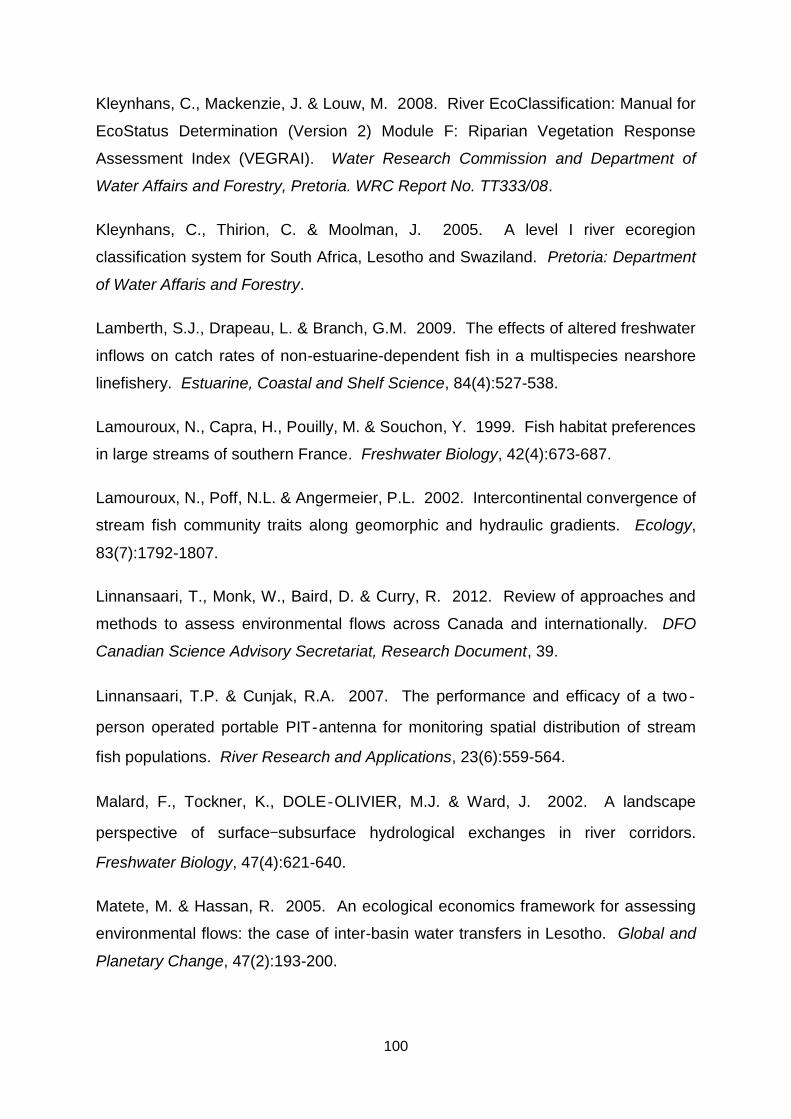
100

Kleynhans, C., Mackenzie, J. & Louw, M. 2008. River EcoClassification: Manual for

EcoStatus Determination (Version 2) Module F: Riparian Vegetation Response

Assessment Index (VEGRAI). Water Research Commission and Department of

Water Affairs and Forestry, Pretoria. WRC Report No. TT333/08.

Kleynhans, C., Thirion, C. & Moolman, J. 2005. A level I river ecoregion

classification system for South Africa, Lesotho and Swaziland. Pretoria: Department

of Water Affaris and Forestry.

Lamberth, S.J., Drapeau, L. & Branch, G.M. 2009. The effects of altered freshwater

inflows on catch rates of non-estuarine-dependent fish in a multispecies nearshore

linefishery. Estuarine, Coastal and Shelf Science, 84(4):527-538.

Lamouroux, N., Capra, H., Pouilly, M. & Souchon, Y. 1999. Fish habitat preferences

in large streams of southern France. Freshwater Biology, 42(4):673-687.

Lamouroux, N., Poff, N.L. & Angermeier, P.L. 2002. Intercontinental convergence of

stream fish community traits along geomorphic and hydraulic gradients. Ecology,

83(7):1792-1807.

Linnansaari, T., Monk, W., Baird, D. & Curry, R. 2012. Review of approaches and

methods to assess environmental flows across Canada and internationally. DFO

Canadian Science Advisory Secretariat, Research Document, 39.

Linnansaari, T.P. & Cunjak, R.A. 2007. The performance and efficacy of a two‐

person operated portable PIT‐antenna for monitoring spatial distribution of stream

fish populations. River Research and Applications, 23(6):559-564.

Malard, F., Tockner, K., DOLE‐OLIVIER, M.J. & Ward, J. 2002. A landscape

perspective of surface–subsurface hydrological exchanges in river corridors.

Freshwater Biology, 47(4):621-640.

Matete, M. & Hassan, R. 2005. An ecological economics framework for assessing

environmental flows: the case of inter-basin water transfers in Lesotho. Global and

Planetary Change, 47(2):193-200.

101

Nel, J.L., Roux, D.J., Maree, G., Kleynhans, C.J., Moolman, J., Reyers, B., et al.

2007. Rivers in peril inside and outside protected areas: a systematic approach to

conservation assessment of river ecosystems. Diversity and Distributions,

13(3):341-352.

O'Brien, G., Swemmer, R. & Wepener, V. 2009. Ecological integrity assessment of

the fish assemblages of the Matigulu/Nyoni and Umvoti estuaries, KwaZulu-Natal,

South Africa. African Journal of Aquatic Science, 34(3):293-302.

Orth, D.J. 1987. Ecological considerations in the development and application of

instream flow‐habitat models. Regulated Rivers: Research & Management,

1(2):171-181.

Oswood, M.W. & Barber, W.E. 1982. Assessment of fish habitat in streams: goals,

constraints, and a new technique. Fisheries, 7(4):8-11.

Pander, J., Mueller, M. & Geist, J. 2013. Ecological functions of fish bypass

channels in streams: migration corridor and habitat for rheophilic species. River

Research and Applications, 29(4):441-450.

Paxton, B.R. 2008. The influence of hydraulics, hydrology and temperature on the

distribution, habitat use and recruitment of threatened cyprinids in a Western Cape

river, South Africa. University of Cape Town.

Paxton, B.R., O'Brien, G.C., Slingsby, J.A. & Copin, R. 2013. Validation of the

periodicity of growth increment deposition in otoliths from the larval and early juvenile

stages of two cyprinids from the Orange–Vaal river system, South Africa. African

Journal of Aquatic Science, 38(sup1):49-54.

Payne, M.M., Council, L.S.W. & High Prairie, A. 2011. Open-Water Hydraulic

Surveys and River2D Modelling.

Perry, J. & Vanderklein, E.L. 2009. Water quality: management of a natural

resource: John Wiley & Sons.

Pollard, S. 2001. Defining flows to protect instream biota: a critique of the instream

flow incremental methodology and the development of a hierarchical habitat-based

102

approach, using the pennant-tailed catlet, Chiloglanis anoterus in the Marite River,

South Africa. University of Cape Town.

Postel, S.L. 2000. Entering an era of water scarcity: the challenges ahead.

Ecological applications, 10(4):941-948.

Power, M.E., Stout, R.J., Cushing, C.E., Harper, P.P., Hauer, F.R., Matthews, W.J.,

et al. 1988. Biotic and abiotic controls in river and stream communities. Journal of

the North American Benthological Society:456-479.

Pusey, B., Storey, A., Davies, P. & Edward, D. 1989. Spatial variation in fish

communities in two South-western Australian River systems. Journal of the Royal

Society of Western Australia JRSUAU, 71(2-3).

Rowntree, K. 1996. The hydraulics of physical biotopes-terminology, inventory and

calibration. WRC Report KV84/96, SBN, 1(86845):229.

Rowntree, K. & Du Plessis, M. 2003. Geomorphological research for the

conservation and management of Southern African rivers, volume 1:

geomorphological impacts of river regulation. Pretoria: Water Research Commission

Report, 849(2):03.

Rowntree, K. & Wadeson, R.A. 1999. A Hierarchical Geomorphological Model for

the Classification of Selected South African Rivers: Final Report to the Water

Research Commission: WRC.

Schlosser, I.J. 1982. Fish community structure and function along two habitat

gradients in a headwater stream. Ecological monographs, 52(4):395-414.

Source-to-Sea, I. Dwaf. 2003. Prepared for the Department of Water Affairs and

Forestry, South Africa. Thukela Water Project Decision Support Phase. Reserve

Determination Study. Pretoria. (PBV000-00-10304).

Southwood, T. 1988. Tactics, strategies and templets. Oikos:3-18.

Sparks, R.E. 1995. Need for ecosystem management of large rivers and their

floodplains. BioScience, 45(3):168-182.

103

Stalnaker, C., Lamb, B.L., Henriksen, J., Bovee, K. & Bartholow, J. 1995. The

instream flow incremental methodology: a primer for IFIM.

Statistics, S. 2013. Mid-year population estimates: Pretoria: sn.

Steffler, P. & Blackburn, J. 2002a. River 2D-Two-Dimensional Depth Averaged

Model of River Hydrodynamics and Fish Habitat Introduction to Depth Averaged

Modeling and User’s.

Steffler, P. & Blackburn, J. 2002b. Two-dimensional depth averaged model of river

hydrodynamics and fish habitat. River2D user’s manual, University of Alberta,

Canada.

Stute, M. 2002. Story line for the B2C groundwater exhibit. Lamont-Doherty Earth

Observatory of Columbia University: Barnard College.

Tennant, D.L. 1976. Instream flow regimens for fish, wildlife, recreation and related

environmental resources. Fisheries, 1(4):6-10.

Ter Braak, C. & Šmilauer, P. 2002. CANOCO and CanoDraw for Windows, version

4.53. Wageningen Univ. and Research Centre, Wageningen, The Netherlands.

Thorp, J.H., Thoms, M.C. & Delong, M.D. 2006. The riverine ecosystem synthesis:

biocomplexity in river networks across space and time. River Research and

Applications, 22(2):123-147.

Van den Brink, P.J., Van den Brink, N.W. & Ter Braak, C.J. 2003. Multivariate

analysis of ecotoxicological data using ordination: demonstrations of utility on the

basis of various examples. Australasian Journal of Ecotoxicology, 9:141-156.

Vannote, R.L., Minshall, G.W., Cummins, K.W., Sedell, J.R. & Cushing, C.E. 1980.

The river continuum concept. Canadian journal of fisheries and aquatic sciences,

37(1):130-137.

Vegter, J., Pitman, W., Xu, Y. & Beekman, H. 2003. Recharge and stream flow.

Groundwater Recharge Estimation in Southern Africa. UNESCO IHP Series(64):109-

123.

104

Vrdoljak, S.M. & Hart, R.C. 2007. Groundwater seeps as potentially important

refugia for freshwater fishes on the Eastern Shores of Lake St Lucia, KwaZulu-Natal,

South Africa. African Journal of Aquatic Science, 32(2):125-132.

Walker, K.F., Sheldon, F. & Puckridge, J.T. 1995. A perspective on dryland river

ecosystems. Regulated Rivers: Research & Management, 11(1):85-104.

Walmsley, R., Walmsley, J. & Silberbauer, M. 1999. Freshwater systems and

resources. National state of the environment Report-South Africa.[Online]

Department of Environmental Affairs and Tourism.

Ward, J. 1998. Riverine landscapes: biodiversity patterns, disturbance regimes, and

aquatic conservation. Biological conservation, 83(3):269-278.

Whitfield, A. & Elliott, M. 2002. Fishes as indicators of environmental and ecological

changes within estuaries: a review of progress and some suggestions for the future.

Journal of Fish Biology, 61(sA):229-250.

Whitfield, A. & Harrison, T. 2003. River flow and fish abundance in a South African

estuary. Journal of Fish Biology, 62(6):1467-1472.

Wohl, E., Cooper, D., Poff, L., Rahel, F., Staley, D. & Winters, D. 2007.

Assessment of stream ecosystem function and sensitivity in the Bighorn National

Forest, Wyoming. Environmental management, 40(2):284-302.

WRI. 2008. Water Scarcity: Private Investment Opportunities in Agricultural Water

Use Efficiency. World Resource Institute.

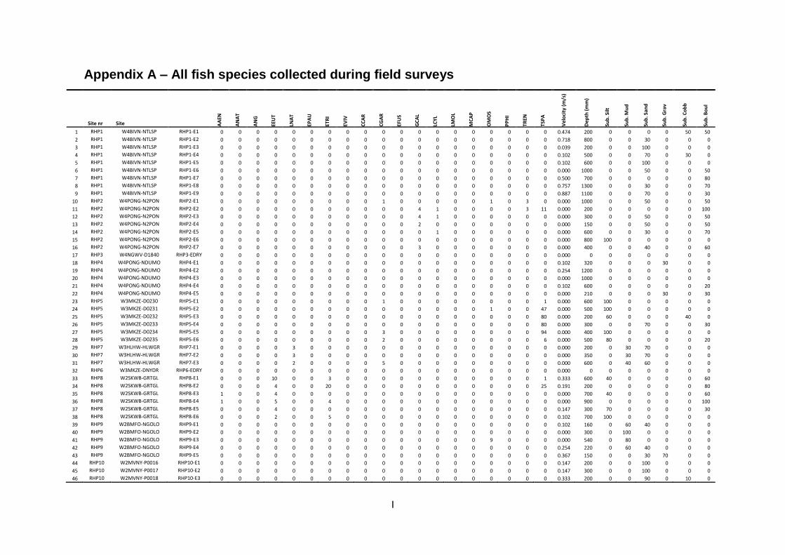
I

Appendix A – All fish species collected during field surveys

Site nr Site

AA

EN

AN

AT

AN

G

EEU

T

LNA

T

EPA

U

ETR

I

EVIV

CC

AR

CG

AR

EFU

S

GC

AL

LCY

L

LMO

L

MC

AP

OM

OS

PP

HI

TREN

TSP

A

Vel

oci

ty (

m/s

)

Dep

th (

mm

)

Sub

. Silt

Sub

. Mu

d

Sub

. San

d

Sub

. Gra

v

Sub

. Co

bb

Sub

. Bo

ul

1 RHP1 W4BIVN-NTLSP RHP1-E1 0 0 0 0 0 0 0 0 0 0 0 0 0 0 0 0 0 0 0 0.474 200 0 0 0 0 50 50









10 RHP2 W4PONG-N2PON RHP2-E1 0 0 0 0 0 0 0 0 0 1 0 0 0 0 0 1 0 3 0 0.000 1000 0 0 50 0 0 50







17 RHP3 W4NGWV-D1840 RHP3-EDRY 0 0 0 0 0 0 0 0 0 0 0 0 0 0 0 0 0 0 0 0.000 0 0 0 0 0 0 0

18 RHP4 W4PONG-NDUMO RHP4-E1 0 0 0 0 0 0 0 0 0 0 0 0 0 0 0 0 0 0 0 0.102 320 0 0 0 30 0 0





23 RHP5 W3MKZE-D0230 RHP5-E1 0 0 0 0 0 0 0 0 0 1 0 0 0 0 0 0 0 0 1 0.000 600 100 0 0 0 0 0

24 RHP5 W3MKZE-D0231 RHP5-E2 0 0 0 0 0 0 0 0 0 0 0 0 0 0 0 1 0 0 47 0.000 500 100 0 0 0 0 0

25 RHP5 W3MKZE-D0232 RHP5-E3 0 0 0 0 0 0 0 0 0 0 0 0 0 0 0 0 0 0 80 0.000 200 60 0 0 0 40 0

26 RHP5 W3MKZE-D0233 RHP5-E4 0 0 0 0 0 0 0 0 0 0 0 0 0 0 0 0 0 0 80 0.000 300 0 0 70 0 0 30

27 RHP5 W3MKZE-D0234 RHP5-E5 0 0 0 0 0 0 0 0 0 3 0 0 0 0 0 0 0 0 94 0.000 400 100 0 0 0 0 0

28 RHP5 W3MKZE-D0235 RHP5-E6 0 0 0 0 0 0 0 0 0 2 0 0 0 0 0 0 0 0 6 0.000 500 80 0 0 0 0 20

29 RHP7 W3HLHW-HLWGR RHP7-E1 0 0 0 0 3 0 0 0 0 0 0 0 0 0 0 0 0 0 0 0.000 200 0 30 70 0 0 0



32 RHP6 W3MKZE-DNYDR RHP6-EDRY 0 0 0 0 0 0 0 0 0 0 0 0 0 0 0 0 0 0 0 0.000 0 0 0 0 0 0 0

33 RHP8 W2SKWB-GRTGL RHP8-E1 0 0 0 10 0 0 3 0 0 0 0 0 0 0 0 0 0 0 1 0.333 600 40 0 0 0 0 60






39 RHP9 W2BMFO-NGOLO RHP9-E1 0 0 0 0 0 0 0 0 0 0 0 0 0 0 0 0 0 0 0 0.102 160 0 60 40 0 0 0





44 RHP10 W2MVNY-P0016 RHP10-E1 0 0 0 0 0 0 0 0 0 0 0 0 0 0 0 0 0 0 0 0.147 200 0 0 100 0 0 0

45 RHP10 W2MVNY-P0017 RHP10-E2 0 0 0 0 0 0 0 0 0 0 0 0 0 0 0 0 0 0 0 0.147 300 0 0 100 0 0 0

46 RHP10 W2MVNY-P0018 RHP10-E3 0 0 0 0 0 0 0 0 0 0 0 0 0 0 0 0 0 0 0 0.333 200 0 0 90 0 10 0

II

Site nr

Continued

AA

EN

AN

AT

AN

G

EEU

T

LNA

T

EPA

U

ETR

I

EVIV

CC

AR

CG

AR

EFU

S

GC

AL

LCY

L

LMO

L

MC

AP

OM

OS

PP

HI

TREN

TSP

A

Vel

oci

ty

(m/s

)

Dep

th (

mm

)

Sub

. Silt

Sub

. Mu

d

Sub

. San

d

Sub

. Gra

v

Sub

. Co

bb

Sub

. Bo

ul

Site

47 RHP11 W2WMFO-DINDI RHP11-E1 0 0 0 0 0 0 0 0 0 0 0 0 0 0 0 1 0 0 0 0.850 300 0 0 80 0 0 20






53 RHP12 W2MFOL-CONFL RHP12-E1 0 0 0 0 0 0 0 0 0 0 0 0 0 0 0 0 0 0 0 0.000 840 0 50 50 0 0 0






59 RHP13 W1MFLE-ELIZB RHP13-E1 0 0 0 0 0 0 0 0 0 1 0 0 0 0 0 0 0 0 0 0.000 400 0 100 0 0 0 0






65 RHP14 W1MHLA-GWEIR RHP14-E1 0 0 0 0 0 0 0 0 0 0 0 0 0 0 0 2 2 0 0 0.038 430 0 0 100 0 0 0









74 RHP15 W1NWKU-MTGLU RHP15-E1 0 0 1 0 0 1 0 0 0 0 0 0 0 0 0 35 18 0 0 0.000 600 0 0 50 50 0 0





79 RHP16 W1EVTH-GINNE RHP16-E1 0 0 0 0 0 0 0 0 0 0 0 0 0 0 0 0 0 0 0 0.000 500 0 50 50 0 0 0






85 RHP17 W1MATI-NYEZA RHP17-E1 0 0 0 0 0 0 0 0 0 0 0 0 0 0 0 0 0 0 48 0.000 200 0 0 100 0 0 0








93 RHP18 V3SLNG NCHTW RHP18-E1 0 0 0 0 0 0 0 0 0 0 0 0 0 0 0 0 0 0 0 0.675 400 0 0 0 0 0 100



III

Site nr

Continued

0 AA

EN

AN

AT

AN

G

EEU

T

LNA

T

EPA

U

ETR

I

EVIV

CC

AR

CG

AR

EFU

S

GC

AL

LCY

L

LMO

L

MC

AP

OM

OS

PP

HI

TREN

TSP

A

Vel

oci

ty

(m/s

)

Dep

th (

mm

)

Sub

. Silt

Sub

. Mu

d

Sub

. San

d

Sub

. Gra

v

Sub

. Co

bb

Sub

. Bo

ul

Site



98 RHP19 V3NCND-LEYDN RHP19-E1 0 0 0 0 0 0 0 0 0 0 0 0 0 0 0 0 0 0 0 0.621 200 0 0 0 0 0 100






104 RHP20 V3BUFF-CONFL RHP20-E1 0 0 0 0 2 0 0 0 1 3 0 0 0 0 0 0 0 0 0 0.411 600 0 0 30 0 0 70









113 RHP21 V3SAND-COTSW RHP21-E1 0 0 0 0 0 0 0 0 0 0 0 0 0 0 0 0 0 0 0 0.102 100 0 0 0 0 0 20





118 RHP22 V1THUK-TUGEL RHP22-E1 0 0 0 0 0 0 0 0 0 0 0 0 0 0 0 0 0 0 0 0.102 500 0 30 0 0 0 70









127 RHP23 V7BUSH-MOORP RHP23-E1 0 0 0 0 8 0 0 0 0 0 0 0 0 0 0 0 0 0 0 0.377 700 0 0 0 0 0 100







134 RHP24 V2UNSP-KMBRG RHP24-E1 0 0 0 0 0 0 0 0 0 0 0 0 0 0 0 0 0 0 0 0.671 350 0 0 0 0 50 50



137 RHP25 V1THUK-RAILB RHP25-E1 0 0 0 0 0 0 0 0 0 0 0 0 0 0 0 0 0 0 0 0.440 300 0 0 0 0 0 0



140 RHP26 U4MVOT-SHANK RHP26-E1 0 0 0 0 0 0 0 0 0 0 0 0 0 0 0 0 0 0 0 0.000 270 0 0 0 0 0 0





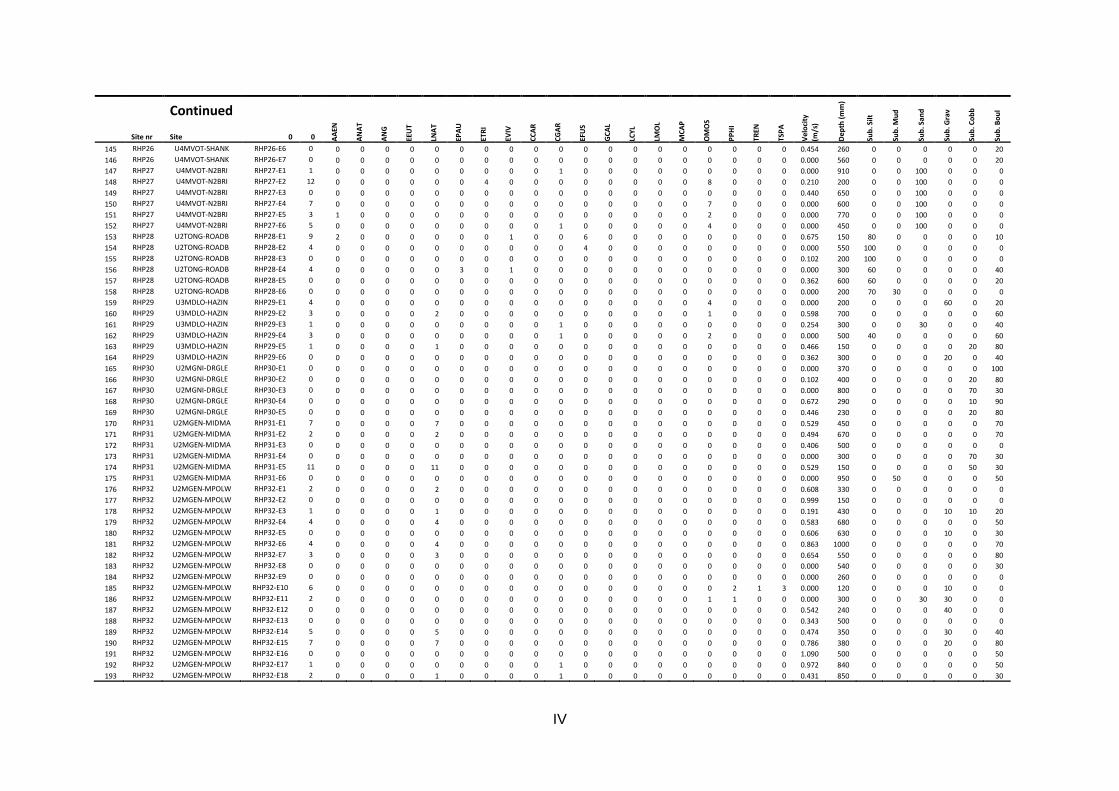
IV

Site nr

Continued

0 0 AA

EN

AN

AT

AN

G

EEU

T

LNA

T

EPA

U

ETR

I

EVIV

CC

AR

CG

AR

EFU

S

GC

AL

LCY

L

LMO

L

MC

AP

OM

OS

PP

HI

TREN

TSP

A

Vel

oci

ty

(m/s

)

Dep

th (

mm

)

Sub

. Silt

Sub

. Mu

d

Sub

. San

d

Sub

. Gra

v

Sub

. Co

bb

Sub

. Bo

ul

Site

145 RHP26 U4MVOT-SHANK RHP26-E6 0 0 0 0 0 0 0 0 0 0 0 0 0 0 0 0 0 0 0 0 0.454 260 0 0 0 0 0 20

146 RHP26 U4MVOT-SHANK RHP26-E7 0 0 0 0 0 0 0 0 0 0 0 0 0 0 0 0 0 0 0 0 0.000 560 0 0 0 0 0 20

147 RHP27 U4MVOT-N2BRI RHP27-E1 1 0 0 0 0 0 0 0 0 0 1 0 0 0 0 0 0 0 0 0 0.000 910 0 0 100 0 0 0






153 RHP28 U2TONG-ROADB RHP28-E1 9 2 0 0 0 0 0 0 1 0 0 6 0 0 0 0 0 0 0 0 0.675 150 80 0 0 0 0 10






159 RHP29 U3MDLO-HAZIN RHP29-E1 4 0 0 0 0 0 0 0 0 0 0 0 0 0 0 0 4 0 0 0 0.000 200 0 0 0 60 0 20






165 RHP30 U2MGNI-DRGLE RHP30-E1 0 0 0 0 0 0 0 0 0 0 0 0 0 0 0 0 0 0 0 0 0.000 370 0 0 0 0 0 100





170 RHP31 U2MGEN-MIDMA RHP31-E1 7 0 0 0 0 7 0 0 0 0 0 0 0 0 0 0 0 0 0 0 0.529 450 0 0 0 0 0 70






176 RHP32 U2MGEN-MPOLW RHP32-E1 2 0 0 0 0 2 0 0 0 0 0 0 0 0 0 0 0 0 0 0 0.608 330 0 0 0 0 0 0


















V

Site nr

Continued

0 AA

EN

AN

AT

AN

G

EEU

T

LNA

T

EPA

U

ETR

I

EVIV

CC

AR

CG

AR

EFU

S

GC

AL

LCY

L

LMO

L

MC

AP

OM

OS

PP

HI

TREN

TSP

A

Vel

oci

ty

(m/s

)

Dep

th (

mm

)

Sub

. Silt

Sub

. Mu

d

Sub

. San

d

Sub

. Gra

v

Sub

. Co

bb

Sub

. Bo

ul

Site

194 RHP32 U2MGEN-MPOLW RHP32-E19 0 0 0 0 0 0 0 0 0 0 0 0 0 0 0 0 0 1 5 0.000 220 0 0 0 0 0 0










204 RHP33 U2MGEN-NINAW RHP33-E1 1 0 0 0 0 0 0 0 0 0 0 0 0 0 0 0 0 0 0 0.000 370 0 0 0 50 0 50







211 RHP35 U6MLAZ-USBAY RHP35-E1 0 0 0 0 0 0 0 0 0 0 0 0 0 0 0 2 0 0 0 0 350 0 0 0 0 0 0




215 RHP35 U6MLAZ-USBAY RHP35-E5 0 0 0 0 0 0 0 0 0 0 0 0 0 0 0 0 0 0 0 0.000 500 100 0 0 0 0 0

216 RHP35 U6MLAZ-USBAY RHP35-E6 0 0 0 0 0 0 0 0 0 0 0 0 0 0 0 0 0 0 0 0.406 160 0 0 0 0 50 50

217 RHP36 U6MLAZ-P0502 RHP36-E1 0 0 0 0 0 0 0 0 0 0 0 0 0 0 0 0 0 0 0 0.377 200 0 0 0 0 0 100

218 RHP36 U6MLAZ-P0503 RHP36-E2 0 0 0 0 0 0 0 0 0 0 0 0 0 0 0 0 0 0 0 0.147 600 30 0 0 0 0 70

219 RHP36 U6MLAZ-P0504 RHP36-E3 0 0 0 0 0 0 0 0 0 0 0 0 0 0 0 0 0 0 0 0.102 600 40 0 0 0 0 60

220 RHP36 U6MLAZ-P0505 RHP36-E4 0 0 0 0 0 0 0 0 0 0 0 0 0 0 0 0 0 0 0 0.631 250 0 0 0 0 0 100

221 RHP36 U6MLAZ-P0506 RHP36-E5 0 0 0 0 0 0 0 0 0 0 0 0 0 0 0 0 0 0 0 0.102 700 40 0 0 0 0 60

222 RHP36 U6MLAZ-P0507 RHP36-E6 0 0 0 0 0 0 0 0 0 0 0 0 0 0 0 0 0 0 0 0.466 400 40 0 0 0 0 60

223 RHP36 U6MLAZ-P0508 RHP36-E7 0 0 0 0 0 0 0 0 0 0 0 0 0 0 0 0 0 0 0 0.000 400 20 0 0 0 0 80

224 RHP37 U6MLAZ-SHONG RHP37-EDNF 0 0 0 0 0 0 0 0 0 0 0 0 0 0 0 0 0 0 0 0.000 0 0 0 0 0 0 0

225 RHP38 U6LOVU-RICHM RHP38-E1 0 0 0 0 0 0 0 0 0 0 0 0 0 0 0 0 0 0 0 0.000 160 0 0 0 0 90 10



228 RHP39 U6LOVU-MIDIL RHP39-EDNF 0 0 0 0 0 0 0 0 0 0 0 0 0 0 0 0 0 0 0 0.000 0 0 0 0 0 0 0

229 RHP40 U6LOVU-KAMPU RHP40-EDNF 0 0 0 0 0 0 0 0 0 0 0 0 0 0 0 0 0 0 0 0.000 0 0 0 0 0 0 0

230 RHP41 U6LOVU-R0197 RHP41-E1 0 0 0 0 0 0 0 0 0 0 0 0 0 0 0 0 0 0 0 0.000 1200 0 0 100 0 0 0

231 RHP41 U6LOVU-R0198 RHP41-E2 0 0 0 0 0 0 0 0 0 0 0 0 0 0 0 1 0 0 0 0.000 800 0 0 100 0 0 0

232 RHP42 U1MKMZ-SANIP RHP42-E1 0 0 0 0 0 0 0 0 0 0 0 0 0 0 0 0 0 0 0 0.557 200 0 0 0 0 0 100



235 RHP43 T5MZIM-NYAMA RHP43-E1 0 0 0 0 0 0 0 0 0 0 0 0 0 0 0 1 0 0 0 0.000 350 0 100 0 0 0 0








VI

Site nr

Continued

0 AA

EN

AN

AT

AN

G

EEU

T

LNA

T

EPA

U

ETR

I

EVIV

CC

AR

CG

AR

EFU

S

GC

AL

LCY

L

LMO

L

MC

AP

OM

OS

PP

HI

TREN

TSP

A

Vel

oci

ty

(m/s

)

Dep

th (

mm

)

Sub

. Silt

Sub

. Mu

d

Sub

. San

d

Sub

. Gra

v

Sub

. Co

bb

Sub

. Bo

ul

Site


244 RHP44 T4MTAM-MADIK RHP44-E1 0 0 0 0 0 0 0 0 0 0 0 0 0 0 0 0 0 0 0 0.000 210 0 0 50 0 0 50










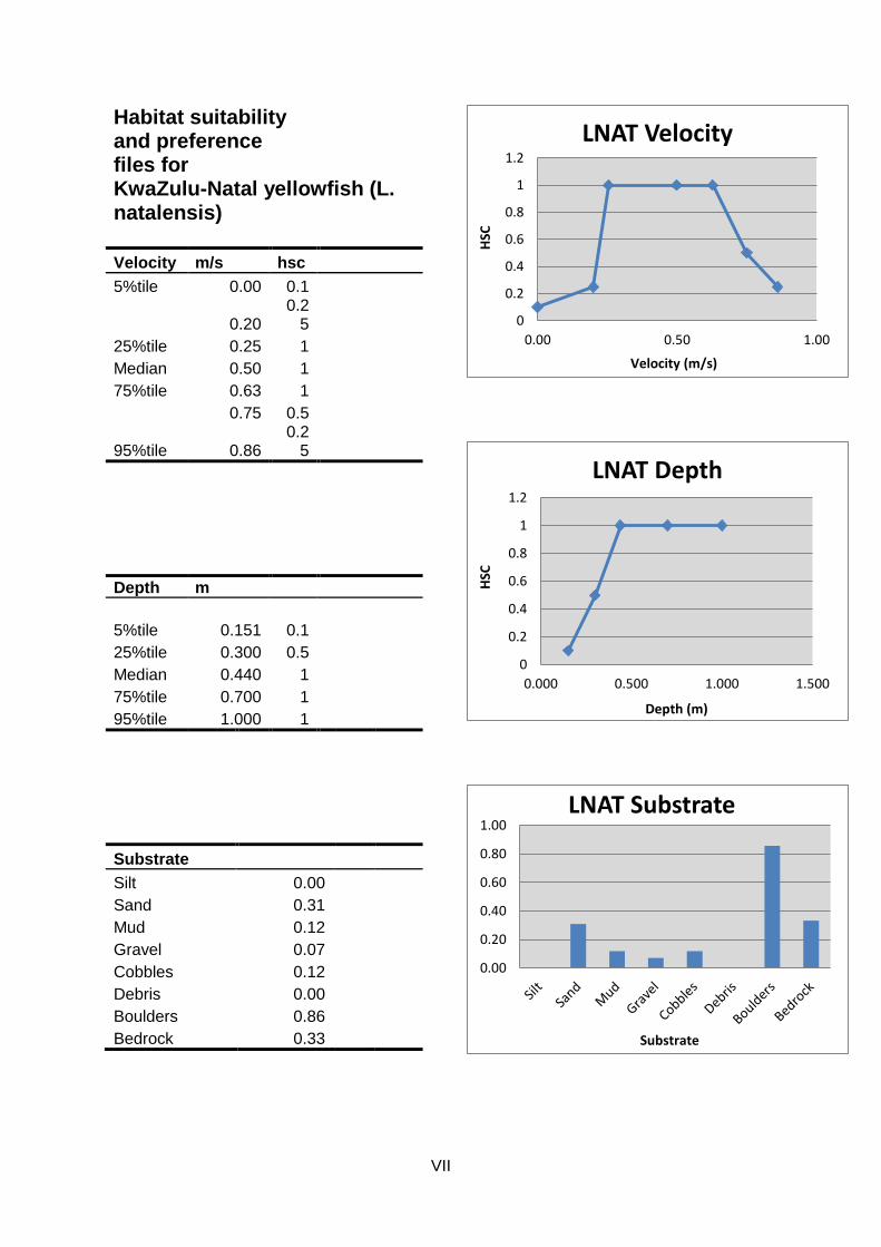
VII

Habitat suitability and preference files for

KwaZulu-Natal yellowfish (L. natalensis)

Velocity m/s hsc 5%tile 0.00 0.1

0.20

0.25

25%tile 0.25 1 Median 0.50 1 75%tile 0.63 1

0.75 0.5

95%tile 0.86

0.25

Depth m

5%tile 0.151 0.1 25%tile 0.300 0.5 Median 0.440 1 75%tile 0.700 1 95%tile 1.000 1

Substrate Silt 0.00

Sand 0.31 Mud 0.12 Gravel 0.07 Cobbles 0.12 Debris 0.00 Boulders 0.86 Bedrock 0.33

0

0.2

0.4

0.6

0.8

1

1.2

0.00 0.50 1.00

HSC

Velocity (m/s)

LNAT Velocity

0

0.2

0.4

0.6

0.8

1

1.2

0.000 0.500 1.000 1.500

HSC

Depth (m)

LNAT Depth

0.00

0.20

0.40

0.60

0.80

1.00

Substrate

LNAT Substrate

VIII

Habitat suitability and preference files for

Dusky sleeper (E. fusca)

Velocity m/s hsc

5%tile 0.00 1

0.00 1

25%tile 0.00 1

Median 0.00 1

75%tile 0.34 1

0.47 0.5

95%tile 0.61 0.25

Depth m

5%tile 0.19 0.1

25%tile 0.35 0.5

Median 0.55 1

75%tile 0.875 1

95%tile 1.135 1

Substrate

Silt 0.67

Mud 0.00

Sand 0.33

Gravel 0.00

Cobbles 0.00

Boulder 0.33

Bedrock 0.33

Debris 0.00

0

0.2

0.4

0.6

0.8

1

1.2

0.00 0.20 0.40 0.60 0.80

HSC

Velocity (m/s)

EFUS Velocity

0

0.2

0.4

0.6

0.8

1

1.2

0 0.5 1 1.5

HSC

Depth (m)

EFUS Depth

0.000.100.200.300.400.500.600.70

Substrate

EFUS Substrate

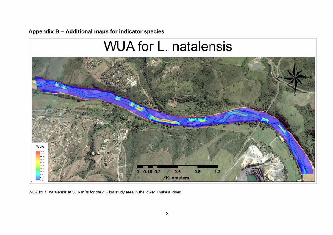
IX

Appendix B – Additional maps for indicator species

WUA for L. natalensis at 50.6 m3/s for the 4.6 km study area in the lower Thukela River.

X

WUA for E. fusca at 50.6 m3/s for the 4.6 km study area in the lower Thukela River.

XI

WUA for L. natalensis at 208 m3/s for the 4.6 km study area in the lower Thukela River.

XII

WUA for E. fusca at 208 m3/s for the 4.6 km study area in the lower Thukela River.

Documents

Hydrological assessment to predict velocity-flow classes