Hydrological Signatures of Earthquake Strainseismo.berkeley.edu/~manga/mwk93.pdf · 22,036 MUIR-WOOD AND KING: HYDROLOGICAL SIGNATURES OF EARTHQUAKE STRAIN quakes can also avalanche

JOURNAL OF GEOPHYSICAL RESEARCH, VOL. 98, NO. B12, PAGES 22,035-22,068, DECEMBER 10, 1993

Hydrological Signatures of Earthquake Strain

ROBERT MUIR-WOOD

EQE International, Clapton, England

GEOFFREY C. P. KING

Institut de Physique du Globe, Strasbourg, France

The character of the hydrological changes that follow major earthquakes has been investigated and found to be dependent on the style of faulting. The most significant response is found to accompany major normal fault earthquakes. Increases in spring and river discharges peak a few days after the earthquake, and typically, excess flow is sustained for a period of 6-12 months. In contrast, hydrological changes accompanying pure reverse fault earthquakes are either undetected or indicate lowering of well levels and spring flows. Strike-slip and oblique-slip fault movements are associated with a mixture of responses but appear to release no more than 10% of the water volume of the same sized normal fault event. For two major normal fault earthquakes in the western United States (those of Hebgen Lake on August 17, 1959, and Borah Peak on October 28, 1983), there is suf•cient river flow information to allow the magnitude and extent of the postseismic discharge to be quantified. The discharge has been converted to a rainfall equivalent, which is found to exceed 100 mm close to the fault and to remain above 10 mm at distances greater than 50 km. The total volume of water released in these earthquakes was around 0.3 km 3 (Borah Peak) and 0.5 km 3 (Hebgen Lake). Qualitative information on other major normal fault earthquakes, in both the western United States and Italy, indicates that the size, duration, and range of their hydrological signatures have been similar. The magnitude and distribution of the water discharge for these events are compared with deformation models calibrated using seismic and geodetic information. The quantity of water released over a time period of 6-12 months suggests that crustal volume strain to a depth of at least 5 km is involved. The rise and decay times of the discharge are shown to be critically dependent on crack widths, and it is concluded that the dominant cracks have a high aspect ratio and cannot be much wider than 0.03 mm. Using the estimated depth to which water is mobilized, the modeled crack size, and the measured volumes of water expelled, it is concluded that even at distances of 50 km from the earthquake epicenters, cracks must be separated by no more than 10 or 20 m. In regions of highest discharge nearer the earthquake epicenters, separations of 1 or 2 m are required. These results suggest that water-filled cracks are ubiquitous throughout the brittle continental crust and that these cracks open and close throughout the earthquake cycle. The existence of tectonically induced fluid flows on the scale that we demonstrate has major implications for our understanding of the mechanical and chemical behavior of crustal rocks.

INTRODUCTION

Hydrological changes associated with earthquakes have been known for more than 2000 years. In the eighteenth and nineteenth centuries, changes in well levels and spring flow attributed to earthquakes were widely reported and were even considered to reflect the processes of earthquake generation. However, in the twentieth century, such ac- counts were discarded as being part of the prescientific earthquake folklore. Richter [1958], for example, does not mention hydrological effects.

The understanding of the causes of liquefaction [Housner, 1958] served to distract attention from reports of hydrological changes, emphasizing the significance of superficial pore pressure increases and water escape, phenomena consequent on cyclic loading of unconsolidated sands. However, if vibration was the chief determinant of the release of water, then an increase in fluvial discharge would simply reflect the extent and severity of ground shaking. However, there is no such relationship. Following the great 1964 Alaska earthquake (Mw 9.25), in the area of strongest ground shaking, water tables were generally lowered and most streams

Copyright 1993 by the American Geophysical Union.

Paper number 93JB02219. 0148-0227/93/93 JB-02219505.00

experienced a decrease in discharge [Waller, 1966]; following the Great San Francisco earthquake of 1906, there were only scattered reports of increases in spring flow in northern California [Lawson, 1908]. In contrast, while the Borah Peak, Idaho, earthquake of 1983 released less than 10% of the energy of the 1906 earthquake and less than 1% of the 1964 Alaska earthquake, its hydrological impact was at least an order of magnitude greater, doubling the flow rates of some rivers for several months. As we will show, the hydrological effects of earthquakes are determined by the style of fault displacement, rather than simply the size of the earthquake.

Superficial or Deep Sources of Earthquake-Induced Water Flow?

While superficial phenomena resulting from ground vibration cannot explain all the earthquake-related hydrological changes, they may on occasion be significant. An increase in fluvial discharge can result from liquefaction and fissure eruption of water formerly stored in unconsolidated near- surface sand layers, as in the north Indian earthquakes of 1897 and 1934, following which large tracts of the alluvial floodplains became covered with water and sand [Oldham, 1899; Dunn et al., 1939]. In regions of high relief, earth-

22,O35

22,036 MUIR-WOOD AND KING: HYDROLOGICAL SIGNATURES OF EARTHQUAKE STRAIN

quakes can also avalanche large quantities of snow to lower elevations, increasing the supply of meltwater. A decrease in discharge commonly results from damming of mountain valleys by landslides and rockfalls. Such phenomena tend either to be short-lived or to have the effect of redistributing the discharge budget, with excess and deficit flow compen- sating for one another over a period of days or weeks. With further research, these characteristics may be corroborated by actual observations of the landslides, avalanches, etc. However, it is commonplace to find downstream observers and earthquake historians inventing such explanations for postseismic changes in fluvial discharge even in the absence of direct observation.

The characteristics of deep source hydrological changes that accompany earthquakes are their extended duration (commonly several months) and the absence of any short- term compensatory adjustment in the hydrological budget once the preseismic hydrological regime has been restored. A deep source for the excess water is unambiguous when the water emerges at a temperature above that of shallow groundwater or has a solute chemistry typical of equilibra- tion with crustal rocks at depth.

Hydrological Measurement

In many continental regions, free from a thick sedimentary cover, unconfined near-surface aquifers extend without interruption into the fractured crystalline rocks of the upper crust. This is revealed by some types of reservoir-induced seismicity for which it is possible to infer a causal connection between an increase in the pore pressures at seismogenic depths and changes in earthquake activity [Simpson et al., 1988]. Correspondingly, changes in pore pressures at depth must have the potential to communicate through to the surface.

Most aquifers discharge through springs, which increase or decrease their flow according to the level of the water table. In general, too little is known of aquifer porosities and the relationship between the superficial water table and its crustal catchment to allow variations in well levels or

individual spring flows to reveal anything other than the "sign" of any change in the flow of water between the superficial water table and the underlying crust. Individual wells or springs may be dominated by the behavior of a single neighboring fracture or set of fractures, whose response may not be typical of the region. However, the product of numerous increases in spring flow can be sampled from river discharge information. By averaging over the area of the watershed, excess river flows fed from surface discharging aquifers reveal the magnitude of water release. This can be expressed in either a linear dimension (in millimeters) or a velocity (in millimeters per day). This "rainfall equivalent discharge," which provides an average of the hydrological effects over large areas, can be readily compared with mechanical-hydrological models of the earthquake process. Where possible, river flow data are used in this paper.

NORMAL FAULT EARTHQUAKES

In the past 35 years there have been three major continental normal fault earthquakes in countries with a well- developed program of hydrological monitoring: the two most recent large normal fault earthquakes in the United States:

the M 7.3 August 17, 1959, Hebgen Lake earthquake in Montana, and the Ms 7.0 October 28, 1983, Borah Peak earthquake 250 km away in Idaho, as well as the Ms 6.9 November 23, 1980, Irpinia, earthquake in southern Italy.

In both Idaho and Montana, surface runoff is dominated by mountain snowmelt in late spring and early summer (May to July), while for the remainder of the year precipitation is low, and river flows are mainly fed from springs. Fortu- itously, both earthquakes occurred in the dry season (Heb- gen Lake in high summer and Borah Peak in the fall) and therefore had a significant impact on fluvial discharge. In contrast, the Italian earthquake occurred in the early part of the wet winter months, in which river flows are dominated by surface water runoff. However, the region to the southwest of the fault rupture comprises a broad limestone plateau which drains through large springs whose flow is not per- turbed by short-term variations in precipitation.

On the left side of Figure 1, flow profiles are shown for rivers in the vicinity of both the Montana and Idaho earthquakes and also from the largest spring close to the Italian earthquake (from information published by the U.S. Geolog- ical Survey (USGS) [1961, USGS (Water Resources Data, Idaho, Water Year 1984), and Salvemini [1982]). All three profiles show the previous year's pattern of flow with a shaded region indicating the difference of flow following the earthquake in relation to the previous year. This excess flow is then replotted to produce the histograms on the right side of Figure 1. These excess flows show a number of common features.

A very significant increase in flow can be seen to have followed each earthquake. At all three measuring gauges the level of discharge rose to levels never previously recorded in the same month over the previous decades of monitoring. The proportional increases in flow of about 200% in Idaho and 40% at both Montana and Italy can of course only be interpreted in the context of the normal flow levels. Precip- itation at both Montana and Italy was below average, both before and after the earthquake; in Idaho, river flows were close to the previous maximum level before the event [Wood et al., 1985a]. In none of the examples was there continued excess precipitation capable of explaining the sustained increase in flow. In each case the flow increased fairly rapidly as compared to the total duration of increased flow, with a risetime of only 4 days in Montana and 10 days in Idaho. The risetime in Italy is somewhat longer and plausibly reflects the lower permeability of the limestone aquifer damping any increase in flow from the underlying crust. The water transit time for rainfall at this spring is 5-6 months [Cotecchia and Salvemini, 1981].

At all three flow gauges, high levels of excess flow have been maintained for a period >6 months. The signature of the excess flow in both Idaho and Montana becomes lost

within the spring snowmelt peak and cannot be traced the following summer. The decline in excess flow appears more nearly linear than exponential, and for this reason we adopt a very simple linear approximation to the decay where we need to extrapolate flow rates with time later in this paper. This conservative approximation tends to underestimate rather than overestimate total flows.

In order to examine both the geographical distribution of the discharge and to determine the flow that could have been expected in the absence of the earthquake, good data coverage is needed. Unfortunately, suitably monitored springs

MUIR-WOOD AND KING: HYDROLOGICAL SIGNATURES OF EARTHQUAKE STRAIN 22,037

Gallatin River near Gallatin Gateway, Montana, USA.

25 I ]' .i:[' Excess flow rate • 15 •:• 5

Aug[i/ •' ....... 0 2 4 6 8 5 Months after ear•qu•e ...... ! ' ' ' ........ I '''' I ' .... 1959 1960 Monks

North Fork of Big Lost River, Idaho, USA. -• 1 Octl28 o •8 o

\ m •;•.,•::.:.:::.?:.:.:.:.:.:.:.:.:.:.:.•

0• , , [ ........... I ' ' '1•84' Months 1983

4

o 2

0 2 4 6 Months after earthquake

Caposele spring, Irpinia, Italy 8

41 ........... I ........... Months 1980 1981

4

2

0

0 2 4 6 8

Months after earthquake

Fig. 1. River and spring flow profiles for the period around the time (arrowed) of three major normal fault earthquakes.

in southern Italy are not widespread, being restricted only to the margins of the limestone massif to the southwest and in the foot wall of the fault. However, the hydrological data from Montana and Idaho are sufficiently comprehensive to attempt to quantify the excess flow and to explore its geographical extent.

Methodology for Examining Postseismic Water Release

It is never possible to know precisely what a river's flow would have been in the absence of the earthquake. How- ever, it is possible to approximate this flow through a variety of strategies that may improve on simply assuming flow would have been the same as the previous year. These include comparison with the monthly averaged flows recorded over a number of years surrounding the date of the earthquake (but not including the year following the event) and comparison with the flows recorded at rivers in the same region but beyond the influence of the earthquake. In the latter case, suitable rivers for comparison should have a similar range of elevations to those contained in the catchment as this can have an important influence both on precipitation induced by topography and the relationship between precipitation and runoff in the winter months.

In regions such as Montana and Idaho, in which the groundwater regime is principally recharged by the spring

snowmelt, the form of the annual flow decay curves, though not their amplitudes, shows considerable year-to-year con- sistency. In most of the detailed hydrological studies reported in this paper, averaged monthly flows obtained over a period of several years around the date of the earthquake are used to obtain the form of the flow curve. The amplitude is then adjusted according to the actual flow immediately prior to the earthquake to produce what we term expected flow curves. A similar procedure is undertaken for rivers in the same region but beyond the influence of the earthquake in order to find out which month's flows were anomalous in

relation to expected flow curves, as derived above. For computing the overall decay curves and cumulative volume of postseismic water release for rivers in the region of the earthquake, such periods of anomalous discharge, once identified, can be avoided. In the detailed studies of postseismic fluvial discharges that follow, these principles are discussed in more detail. To avoid confusion associated with

calender dates (the way in which the source information is published), we also quote time as days or months postearth- quake: PE.

August 17, 1959, Hebgen Lake Earthquake

In Figure 2, three river flow profiles are shown for the region around Hebgen Lake, Montana. Daily flow informa-


•ous •u!•d•

!IOta •ous

aos iod•m

3os •od•m

!IOta •ous

lIom •ous :•u!•d S

3os •odtm

3os lod t uI olin •oIz I

l[om •ous

!IOta •ous õu!•d s

oos •odtm Ole• •oI: t

aos •od•m o•m •oId


tion, available for the period July to mid-October 1959 (taken from Stermitz [1964]), is shown on the left, while monthly records of flow data for the period 1958-1961 [from USGS, 1961] are plotted on the right. For both sets of plots the average monthly flows for the period 1950-1965 [from USGS, 1961, 1966] are shown for comparison (excluding August 1959 to July 1960 following the earthquake). From the daily plots it can be seen that in all three rivers, a peak in flow arrived within 4 days of the earthquake and that the increase in flow remained nearly undiminished for at least 60 days. Toward the end of this period the record becomes slightly disturbed by rainfall events, with short-duration spikes.

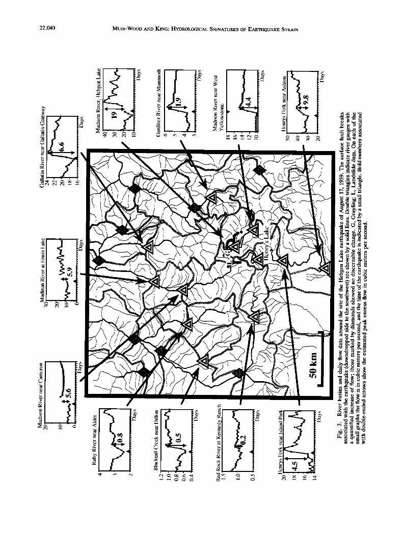
River flow (in cubic meters per second) was measured at many gauges in the region around the earthquake, as indicated in Figure 3, a map of the rivers. The double triangles indicate those locations for which the changes associated with the earthquake are quantified, and diamonds indicate gauges which exhibited no clear changes [Stermitz, 1964]. The data associated with each of the gauged rivers showing an increase in flow are plotted in small graphs around the map. Three of the profiles are derived indirectly: Madison River at Hebgen Lake; Madison River at Ennis Lake, and Henry's Fork River at Island Park Reservoir. For these, computed values of flow were published by Stermitz based on the relationship between reservoir water levels and known discharges. The flow data for Madison River near Cameron prior to the earthquake were also derived indirectly by Stermitz from comparison with flow data at this and other gauges along Madison River in previous years. However, after a week following the earthquake the flow at Cameron was measured directly.

Increases in flow rates (in cubic meters per second) following the earthquake, obtained by subtracting the flow on August 17 (immediately before the earthquake) from that on August 21 (+4 days PE), are shown for each profile. As the trend of summer flows is declining, such a procedure presumably provides a small underestimate of the actual increase in flow. For Madison River at Hebgen Lake (in the catchment that includes most of the surface fault breaks) there appeared to be a marked increase in flow in advance of the earthquake, and the preearthquake flow has been taken as the average of the values for August 16 and 17.

Some of the determinations of additional flow for the

period following the earthquake require further explanation. Hebgen Lake, located in the immediate hanging wall of the fault, was tilted and decreased in capacity at the time of the earthquake, losing a significant quantity of water over the dam. The figures for the input to the lake in the 2 days following the earthquake are consequently seriously dis- torted by these changes and have been omitted. Ten kilometers below the Hebgen Dam, Madison River became blocked by a 21 x 10 6 m 3 landslide triggered by the earthquake. Over a period of 3 weeks this natural dam caused a lake (60 m deep) to fill until it overtopped and rapidly eroded. For this 3-week period, flow at the gauge near Cameron and farther downstream below Ennis Lake accumulated only from the Madison River catchment below the slide. Cabin Creek and

Beaver Creek join Madison River between the river gauge at Grayling and the landslide dam. Hence the flow between Grayling and Cameron before the earthquake includes a contribution from these side streams, while the flow following the earthquake does not. As these streams were not

gauged before the earthquake, their contribution can only be assessed from a comparison with the flow emerging from neighboring watersheds, in the same terrain. On August 17, immediately prior to the earthquake, for each square kilometer of catchment, Hebgen Lake received 7.38 L s -j, Gallatin River received 7.78 L s -j , and Gardiner River received 7.28 L s -•. The average value across all these catchments was 7.54 L s -• km -2. Using this value for the 181 km 2 combined Cabin Creek and Beaver Creek drainages gives an estimated preearthquake flow of 1.367 m 3 s -• into Madison River. Hence the flow assessed to enter Madison

River between the Grayling and Cameron gauges immediately before the earthquake has been reduced by this amount in order to determine the increase in flow for the drainage basin between the landslide dam and Cameron following the earthquake. On the flowcharts in Figure 3, the flow indicated prior to the earthquake for both Cameron and Ennis Lake is modified to show only that component of the overall flow that came from the catchment below Hebgen Lake (achieved by deducting the daily flow immediately below the Hebgen Dam at Grayling from that recorded farther downstream). As the normal flow in Madison River took 2-3 days to drain through Cameron and Ennis Lake, before the interruption at the Madison River slide took effect, for these downriver locations, flow data have not been plotted from the time of the earthquake until August 21.

Figure 4 shows values of peak excess flow normalized over the area of the individual catchments and expressed in terms of daily rainfall equivalents (in millimeters per day). Wherever there is more than one flow gauge on the same river, drainage basins have been subdivided: for example, excess flow on Madison River near Cameron has been

subtracted from the excess flow at Ennis Lake, and excess flow on the Henry's Fork near Island Park reservoir has been subtracted downstream near Ashton. Peak excess flow

for the small Henry's Lake drainage basin in the headwaters of Henry's Fork (0.35 mm/d) is taken from information published separately by Stermitz [1964]. Normalized rainfall equivalent values of excess flow range from 1.33 mm/d in the Hebgen Lake catchment close to the fault down to 0.02 mm/d in the Red Rock River catchment 50 km to the west of

the surface fault breaks. In this and later figures the peak equivalent rainfall values are banded in three shades to allow ready comparison with later strain models.

To explore the duration of excess discharge, it is necessary to have uncontaminated flow data. This disqualifies discharge information from a number of rivers around Heb- gen Lake. From the first week of September 1959, discharge in Madison River below Hebgen Lake became affected by overtopping of the Madison River slide and subsequently by the drawdown of the Hebgen Lake reservoir to inspect damage to the dam. In the Henry's Fork drainage basin, flow was significantly manipulated by irrigation, while in Ruby River, Blacktail Creek, and Red Rock Rivers, the excess flow signal was considered too small to be followed for many months. This leaves the flow data for the gauges already presented in Figure 2: Madison River at West Yellowstone, Gallatin River at Gallatin Gateway, and Gardiner River at Mammoth. As explained earlier, the expected flow is assumed to have the form of the average annual decay curve calibrated using the fluvial discharge immediately before the earthquake. For Gallatin River it can be seen from Figure 2 that prior to the earthquake, flows were closely similar to



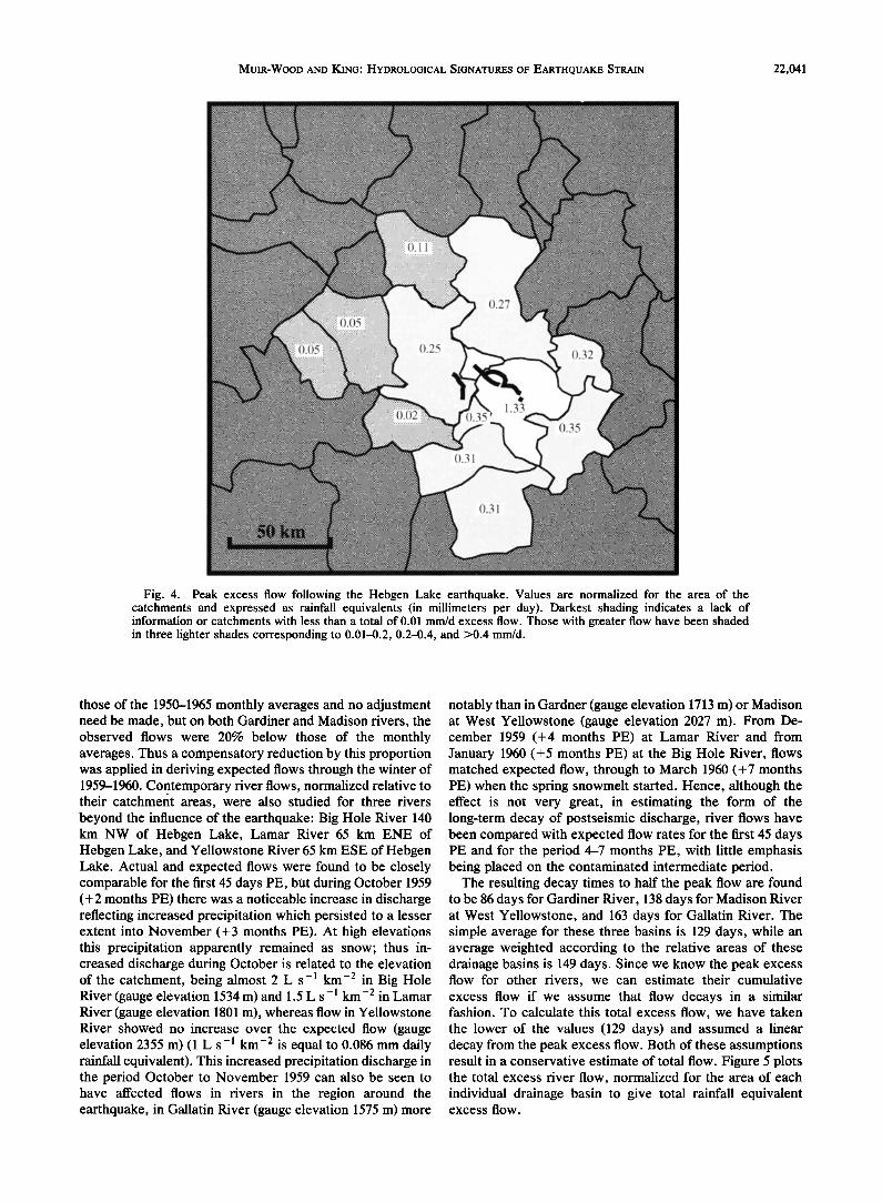
Fig. 4. Peak excess flow following the Hebgen Lake earthquake. Values are normalized for the area of the catchments and expressed as rainfall equivalents (in millimeters per day). Darkest shading indicates a lack of information or catchments with less than a total of 0.01 mm/d excess flow. Those with greater flow have been shaded in three lighter shades corresponding to 0.01-0.2, 0.2-0.4, and >0.4 mm/d.

those of the 1950-1965 monthly averages and no adjustment need be made, but on both Gardiner and Madison rivers, the observed flows were 20% below those of the monthly averages. Thus a compensatory reduction by this proportion was applied in deriving expected flows through the winter of 1959-1960. Contemporary river flows, normalized relative to their catchmerit areas, were also studied for three rivers beyond the influence of the earthquake: Big Hole River 140 km NW of Hebgen Lake, Lamar River 65 km ENE of Hebgen Lake, and Yellowstone River 65 km ESE of Hebgen Lake. Actual and expected flows were found to be closely comparable for the first 45 days PE, but during October 1959 (+ 2 months PE) there was a noticeable increase in discharge reflecting increased precipitation which persisted to a lesser extent into November (+3 months PE). At high elevations this precipitation apparently remained as snow; thus increased discharge during October is related to the elevation of the catchment, being almost 2 L s -l km -2 in Big Hole River (gauge elevation 1534 m) and 1.5 L s -• km -2 in Lamar River (gauge elevation 1801 m), whereas flow in Yellowstone River showed no increase over the expected flow (gauge elevation 2355 m) (1 L s -• km -2 is equal to 0.086 mm daily rainfall equivalent). This increased precipitation discharge in the period October to November 1959 can also be seen to have affected flows in rivers in the region around the earthquake, in Gallatin River (gauge elevation 1575 m) more

notably than in Gardner (gauge elevation 1713 m) or Madison at West Yellowstone (gauge elevation 2027 m). From De- cember 1959 (+4 months PE) at Lamar River and from January 1960 (+5 months PE) at the Big Hole River, flows matched expected flow, through to March 1960 (+7 months PE) when the spring snowmelt started. Hence, although the effect is not very great, in estimating the form of the long-term decay of postseismic discharge, river flows have been compared with expected flow rates for the first 45 days PE and for the period 4-7 months PE, with little emphasis being placed on the contaminated intermediate period.

The resulting decay times to half the peak flow are found to be 86 days for Gardiner River, 138 days for Madison River at West Yellowstone, and 163 days for Gallatin River. The simple average for these three basins is 129 days, while an average weighted according to the relative areas of these drainage basins is 149 days. Since we know the peak excess flow for other rivers, we can estimate their cumulative excess flow if we assume that flow decays in a similar fashion. To calculate this total excess flow, we have taken the lower of the values (129 days) and assumed a linear decay from the peak excess flow. Both of these assumptions result in a conservative estimate of total flow. Figure 5 plots the total excess river flow, normalized for the area of each individual drainage basin to give total rainfall equivalent excess flow.


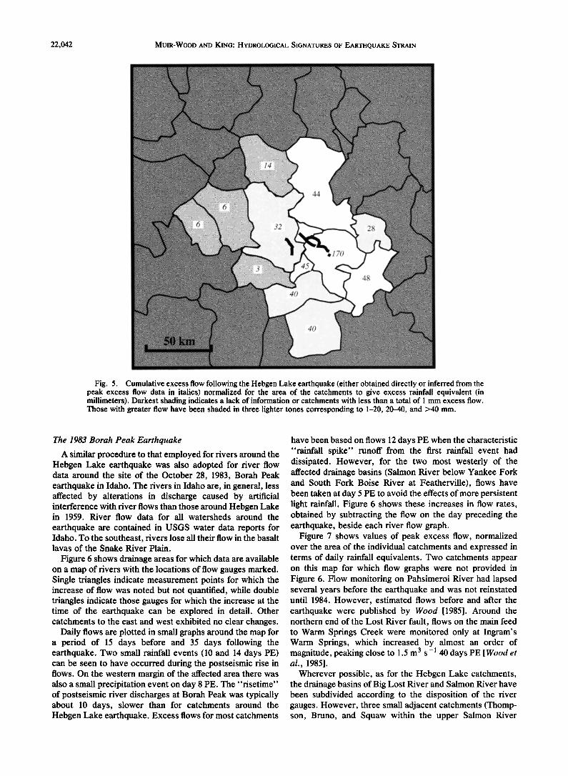
Fig. 5. Cumulative excess flow following the Hebgen Lake earthquake (either obtained directly or inferred from the peak excess flow data in italics) normalized for the area of the catchments to give excess rainfall equivalent (in millimeters). Darkest shading indicates a lack of information or catchments with less than a total of 1 mm excess flow. Those with greater flow have been shaded in three lighter tones corresponding to 1-20, 20-40, and >40 mm.

The 1983 Borah Peak Earthquake

A similar procedure to that employed for rivers around the Hebgen Lake earthquake was also adopted for river flow data around the site of the October 28, 1983, Borah Peak earthquake in Idaho. The rivers in Idaho are, in general, less affected by alterations in discharge caused by artificial interference with river flows than those around Hebgen Lake in 1959. River flow data for all watersheds around the

earthquake are contained in USGS water data reports for Idaho. To the southeast, rivers lose all their flow in the basalt lavas of the Snake River Plain.

Figure 6 shows drainage areas for which data are available on a map of rivers with the locations of flow gauges marked. Single triangles indicate measurement points for which the increase of flow was noted but not quantified, while double triangles indicate those gauges for which the increase at the time of the earthquake can be explored in detail. Other catchments to the east and west exhibited no clear changes.

Daily flows are plotted in small graphs around the map for a period of 15 days before and 35 days following the earthquake. Two small rainfall events (10 and 14 days PE) can be seen to have occurred during the postseismic rise in flows. On the western margin of the affected area there was also a small precipitation event on day 8 PE. The "risetime" of postseismic river discharges at Borah Peak was typically about 10 days, slower than for catchments around the Hebgen Lake earthquake. Excess flows for most catchments

have been based on flows 12 days PE when the characteristic "rainfall spike" runoff from the first rainfall event had dissipated. However, for the two most westerly of the affected drainage basins (Salmon River below Yankee Fork and South Fork Boise River at Featherville), flows have been taken at day 5 PE to avoid the effects of more persistent light rainfall. Figure 6 shows these increases in flow rates, obtained by subtracting the flow on the day preceding the earthquake, beside each river flow graph.

Figure 7 shows values of peak excess flow, normalized over the area of the individual catchments and expressed in terms of daily rainfall equivalents. Two catchments appear on this map for which flow graphs were not provided in Figure 6. Flow monitoring on Pahsimeroi River had lapsed several years before the earthquake and was not reinstated until 1984. However, estimated flows before and after the earthquake were published by Wood [1985]. Around the northern end of the Lost River fault, flows on the main feed to Warm Springs Creek were monitored only at Ingram's Warm Springs, which increased by almost an order of magnitude, peaking close to 1.5 m3 s- 1 40 days PE [Wood et al., 1985].

Wherever possible, as for the Hebgen Lake catchments, the drainage basins of Big Lost River and Salmon River have been subdivided according to the disposition of the river gauges. However, three small adjacent catchments (Thomp- son, Bruno, and Squaw within the upper Salmon River



winter, flows were lower than expected, in December 1983 (+2 months PE) down by 1-2 L s -l km -2, in January 1984 (+3 months PE) down by 0.7-1.2 L s -l km -2, and in February 1984 (+4 months PE) down 1.6-3.3 L s -l km -•. In order to explore the decay of excess flow in catchments around the earthquake, gauged flows were compared with expected values over the most consistent period from De- cember 1983 to January 1984.

Figure 8 plots the total excess river flow, normalized for the area of each individual drainage basin as total rainfall equivalent excess flow. The value for Warm Springs Creek at Challis is based only on the excess flow during the first year, as the increase in discharge persisted for several years. The value for Pahsimeroi River has been inferred from the

flow curve published by Wood [1985]. Figure 8 has the same shading intervals and may be compared with Figure 5 for the Hebgen Lake earthquake.

Discussion of Hebgen Lake and Borah Peak Earthquakes and Examples of Other Normal Fault Events

The maps for Hebgen Lake (Figures 3, 4, and 5) and Borah Peak (Figures 6, 7, and 8) have been plotted at consistent scales and show a number of similarities. With increasing distance from the fault there is a decline in the magnitude of the hydrological impact of the earthquake, although it re-

Fig. 7. Peak excess flow following the Borah Peak earthquake. Values are normalized for the area of the catchments and expressed as rainfall equivalents (in millimeters per day). Darkest shading indicates a lack of information or catchments with less than a total

of 0.01 mm/d excess flow. Those with greater flow have been shaded in three lighter tones corresponding to 0.01-0.2, 0.2-0.4, and >0.4 mm/d. Values in parentheses are from estimated flows.

basin) have, for simplicity, been compounded. In order to be able to compile information for Big Lost River at Mackay the river gauge flows have been adjusted to allow for the daily change in the recorded volume of water stored in Mackay Reservoir immediately upstream. However, these adjusted values are still likely to be underestimated because the alluvial plain of the Big Lost River valley is broad and a proportion of excess discharge is known from well observations to have raised the water table rather than increased

river flows [Whitehead et al., 1984]. Figure 7 shows values of peak excess discharge that can

be seen to range up to 0.61 mm/d in the North Fork of Big Lost River in the hanging wall of the fault. Peak equivalent rainfall values have been banded in three shades consistent

with those employed in Figure 4. To examine the duration of flow, the average monthly

values for all of the catchments were found for the decade of

water years 19'76-1985 (neglecting the year following the earthquake) (USGS, Water Resources Data, Idaho, 1976- 1985), and these were converted into expected flows using data from September 1983 a month before the earthquake. A study was also undertaken of contemporary flows in two rivers beyond the influence of the earthquake: Little Salmon River at Riggins (240 km NW of the epicentre) and Boise River at Twin Springs (160 km WSW of the epicenter). In both these rivers during November (+ 1 month PE) there was an increase in precipitation runoff of about 3 L s -1 km -2 relative to expected values. Throughout the remainder of the

Fig. 8. Cumulative excess flow following the Borah Peak earthquake (either obtained directly or inferred from the peak excess flow data) normalized for the area of the catchments to give excess rainfall equivalent (in millimeters). Darkest shading indicates a lack of information or catchments with less than a total of I mm excess

flow. Those with greater flow have been shaded in three lighter tones corresponding to 1-20, 20-40, and >40 mm. Values in parentheses are from estimated flows.


mains detectable at distances of at least 50 km. The highest values of rainfall equivalent, found in the vicinity of the fault, are greater than 80 mm. By adding together all the separate excess flows for these two earthquakes an estimate can be made of the total volume of fluid release. The

individual excess flows sum to 0.3 km 3 for the Borah Peak earthquake and to 0.5 km3 for the Hebgen Lake earthquake. Uncertainties in estimating the form and duration of the excess flow mean that these values have fairly broad confi- dence bounds but for reasons discussed earlier are probably underestimates.

In order to see whether the hydrological signatures of these two normal fault earthquakes were somehow a product of the particular geology or topography of this region of the northwestern United States, we now discuss some other continental normal fault earthquakes for which information on hydrological changes is available. In general, this information exists simply in a qualitative form, and (with one exception) reporting is rarely continued for a sufficient period to assess the duration of any hydrological response. However, the available evidence suggests that the features we have described are common to all normal faulting events.

Prior to the Hebgen Lake earthquake there have been three magnitude 7 normal fault earthquakes in the Basin and Range province since the late nineteenth century: the 1954 Dixie Valley and 1915 Pleasant Valley earthquakes, both in Nevada and the 1887 Sonora earthquake south of the Ari- zona border in Mexico.

Some descriptions of the hydrological effects of the M 6.9 [Bell and Katzer, 1990] Dixie Valley earthquake, on Decem- ber 16, 1954, were published by Zones [1957], who made a visit to the only part of the fault that was easily accessible by road. "Two weeks after the earthquake a large volume of water had flowed from wells and springs and water stood in many of the fields. Part of the water standing in the playa was probably snowmelt, but a large part of it undoubtedly was ground water that had flowed to the playa from wells and springs and possibly from openings in the ground" [Zones, 1957, p. 389]. In Dixie Valley "the water level in every non-flowing well that was measured was higher after the earthquake" [Zones, 1957, p. 391]. "As a result of the earthquake the flow from many wells temporarily increased and several wells that had not flowed before the earthquake flowed for more than a month" [Zones, 1957, p. 391]. Much of this region of central Nevada was entirely uninhabited, and the extent of such water discharge, beyond Dixie Valley, remains unreported. However, the flow of well 7 in Dixie

litres /see

30 ell 7

20

......... ..........

Fig. 9. Near-fault spring flows monitored following the Dixie Valley earthquake of December 16, 1954.

1887 Sonora

Earthquake

Fig. 10. Hydrological effects of the Sonora earthquake of May 3, 1887. River basins with significant increases of flow are identified by lighter shading and triangles indicate increased river flows. The route taken by B. MacDonald is identified by a striped line. The surface fault break, marked by a thick line, was downdropped to the west.

Valley and from Mud Springs (at the bedrock-alluvium contact at the base of the Stillwater Range) was measured at infrequent intervals over a period of 18 months (see Figure 9). For well 7, after a sharp increase following the earthquake, there was a rapid decline in flow, although both 6 weeks after the event and at the end of the observation

period, flow remained 5 times greater than before. Excess discharge at Mud Springs declined far more slowly, after 18 months being still more than an order of magnitude greater than before the earthquake.

A brief description of the effects of the Pleasant Valley earthquake is given by Jones [1915, p. 197], who notes

One of the most striking effects of the earthquake was the large increase in the flow of streams and springs throughout the northern part of Nevada. In Pleasant Valley all of the streams issuing from the Sonoma Range trebled or quadrupled their flow, until water had stood on the playas, a circumstance that had not been known to happen at this time of year before.

The increase in flow of the streams and the breaking out of new springs was such a common occurrence in the area within fifty miles of the origin of the earthquake that the office of the State Engineer received over fifty applications for the new water rights.

The Sonora earthquake of May 3, 1887 (Figure 10), produced 75 km of fault scarps [Sumner, 1977; Bull and Pearthree, 1988] and was probably the largest of all the


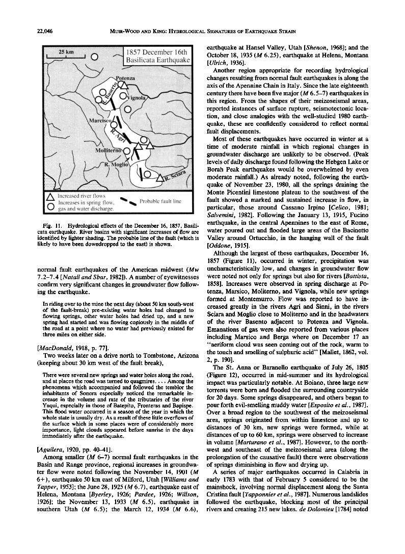
Fig. I I. Hydrological effects of the December 16, 1857, Basili- cata earthquake. River basins with significant increases of flow are identified by lighter shading. The probable line of the fault (which is likely to have been downdropped to the east) is shown.

normal fault earthquakes of the American midwest (Mw 7.2-7.4 [Natali and $bar, 1982]). A number of eyewitnesses confirm very significant changes in groundwater flow following the earthquake.

In riding over to the mine the next day (about 50 km south-west of the fault-break) pre-existing water holes had changed to flowing springs, other water holes had dried up, and a new spring had started and was flowing copiously in the middle of the road at a point where no water had previously existed for three miles on either side.

[MacDonald, 1918, p. 77]. Two weeks later on a drive north to Tombstone, Arizona

(keeping about 30 km west of the fault break),

There were several new springs and water holes along the road, and at places the road was turned to quagmires .... Among the phenomena which accompanied and followed the temblor the inhabitants of Sonora especially noticed the remarkable increase in the volume and rate of the tributaries of the river

Yaqui, especially in those of Batepito, Fronteras and Bapispe. This flood water occurred in a season of the year in which the whole state is usually dry. As a result of these little overflows of the surface which in some places were of considerably more importance, light clouds appeared before sunrise in the days immediately after the earthquake.

[Aguilera, 1920, pp. 40-41]. Among smaller (M 6-7) normal fault earthquakes in the

Basin and Range province, regional increases in groundwater flow were noted following the November 14, 1901 (M 6+), earthquake 50 km east of Milford, Utah [Williams and Tapper, 1953]; the June 28, 1925 (M 6.7), earthquake east of Helena, Montana [Byerley, 1926; Pardee, 1926; Willson, 1926]; the November 13, 1933 (M 6.5), earthquake in southern Utah (M 6.5); the March 12, 1934 (M 6.6),

earthquake at Hansel Valley, Utah [Shenon, 1968]; and the October 18, 1935 (M 6.25), earthquake at Helena, Montana [Ulrich, 1936].

Another region appropriate for recording hydrological changes resulting from normal fault earthquakes is along the axis of the Apennine Chain in Italy. Since the late eighteenth century there have been five major (M 6.5-7) earthquakes in this region. From the shapes of their meizoseismal areas, reported instances of surface rupture, seismotectonic location, and close analogies with the well-studied 1980 earthquake, these are confidently considered to reflect normal fault displacements.

Most of these earthquakes have occurred in winter at a time of moderate rainfall in which regional changes in groundwater discharge are unlikely to be observed. (Peak levels of daily discharge found following the Hebgen Lake or Borah Peak earthquakes would be overwhelmed by even moderate rainfall.) As already noted, following the earthquake of November 23, 1980, all the springs draining the Monte Picentini limestone plateau to the southwest of the fault showed a marked and sustained increase in flow, in particular, those around Cassano Irpino [Celico, 1981; Salvemini, 1982]. Following the January 13, 1915, Fucino earthquake, in the central Apennines to the east of Rome, water poured out and flooded large areas of the Bacinetto Valley around Ortucchio, in the hanging wall of the fault [Oddone, 1915].

Although the largest of these earthquakes, December 16, 1857 (Figure 11), occurred in winter, precipitation was uncharacteristically low, and changes in groundwater flow were noted not only for springs but also for rivers [Battista, 1858]. Increases were observed in spring discharge at Po- tenza, Marsico, Moliterno, and Vignola, while new springs formed at Montemurro. Flow was reported to have increased greatly in the rivers Agri and Sinni, in the rivers Sciara and Moglio close to Moliterno and in the headwaters of the river Basento adjacent to Potenza and Vignola. Emanations of gas were also reported from various places including Marsico and Berga where on December 17 an "aeriform cloud was seen coming out of the rock, warm to the touch and smelling of sulphuric acid" [Mallet, 1862, vol. 2, p. 190].

The St. Anna or Baranello earthquake of July 26, 1805 (Figure 12), occurred in mid-summer and its hydrological impact was particularly notable. At Boiano, three large new torrents were born and flooded the surrounding countryside for 20 days. Some springs disappeared, and others began to pour forth evil-smelling muddy water [Esposito et al., 1987]. Over a broad region to the southwest of the meizoseismal area, springs originated from within limestone and up to distances of 30 km, new springs were formed, while at distances of up to 60 km, springs were observed to increase in volume [Marturano et al., 1987]. However, to the northwest and southeast of the meizoseismal area (along the prolongation of the causative fault) there were observations of springs diminishing in flow and drying up.

A series of major earthquakes occurred in Calabria in early 1783 with that of February 5 considered to be the mainshock, involving normal displacement along the Santa Cristina fault [Tapponnier et al., 1987]. Numerous landslides followed the earthquake, blocking most of the principal rivers and creating 215 new lakes. de Dolomieu [1784] noted


Springs dried up

Fig. 12. Hydrological effects of the July 26, 1805, Baranello earthquake. The probable line of the fault (assumed to have been downdropped to the east) is shown.

that the springs were all flowing more strongly following the earthquake.

REVERSE FAULT EARTHQUAKES

The hydrological changes that accompany reverse fault earthquakes are most notable by their absence. While the number of reverse fault earthquakes occurring in regions of well-developed hydrological monitoring is not as large as for normal faults, there are a number of well-documented examples. These examples are consistent in showing that for earthquakes with purely reverse displacement there are no equivalents to the ubiquitous and widespread reports of water expulsion found for normal fault events. Large continental reverse fault earthquakes have occurred in a number of continental regions, most notably Algeria, Iran, Taiwan, Australia, and Japan.

In a survey of historical earthquakes in the Algiers region (an area dominated by reverse faulting) in three out of six damaging nineteenth century earthquakes, springs of water dried up [Ambraseys and Vogt, 1988]. In all mention of hydrological changes that accompanied earthquakes throughout the historical period in Algiers, falling wells and drying springs are the only phenomena recorded.

In Iran, following the largest continental reverse fault earthquake of the past few decades at Tabas on September 16, 1978, an earthquake which involved widespread surface fault rupture, no hydrological changes were reported [e.g., Ambraseys and Melville, 1982]. Hydrological changes are, however, frequently reported accompanying other, generally strike-slip or oblique-slip earthquakes in Iran.

Continental reverse fault activity also predominates in Taiwan, where observations of gas well pressures were

made before and after the Ms 6.75 January 18, 1964, earthquake [Wu, 1975]. In the footwall of the fault a reduction in pressure occurred after the earthquake; in the hanging wall a reduction had begun 9 months before the earthquake, although loss of a production well prevents quantification of those changes that accompanied the earthquake.

A number of major reverse fault earthquakes involving surface fault rupture have also occurred in the past 25 years in central and western Australia. Although a rise in water levels in boreholes near Perth was originally considered to have preceded and accompanied the M 6.8 Meckering earthquake 130 km away in western Australia [Gordon, 1970], this was later shown to have been the result of rainfall [Gregson et al., 1976]. The January 22, 1988, Ms 6.3-6.7 Tennant Creek earthquakes occurred in the vicinity of some water extraction boreholes but no changes in water levels were noted by Bowman et al. [1990].

The M 7.2 1896 Rikuu (North Honshu) Reverse Fault Earthquake

The Rikuu (North Honshu) earthquake of August 31, 1896, involved significant surface fault rupture, over a distance of about 36 km with a maximum uplift of 3.5 m and a displacement of about 5 m [Matsuda et al., 1980]. This was accompanied by an antithetic reverse fault motion some 15 km to the east in the hanging wall of the main fault. No changes in river flows were reported following the earthquake. How- ever, this region of northern Honshu has many hot springs, and a number were affected by the event [Yamasaki, 1900]. Hot springs supplying bathhouses at Oshuku, Tsunagi, and Osawa dried up after the earthquake, while there was a significant reduction in flow at the springs at Namari and Yuda. All of these lie in the hanging wall of the main fault, to the east, and within 20 km of the principal antithetic fault, in the region that is subject to increases in spring and river flows in an equivalent normal fault earthquake. In contrast, following the earthquake, a new hot spring formed at Segan- Toge on the flank of a volcano close to the northern end of the main fault.

In North America (blind) reverse fault earthquakes are found around the central section of the San Andreas fault,

the largest in the past 30 years being that at Coalinga (M 6.2) on May 2, 1983. Changes in hydrocarbon fluid pressures and well levels were reported anecdotally to have occurred, but the results have not been made public [see Sega# and Yerkes, 1990]. However, in the nearby M 5.5 Kettleman Hills earthquake, falls in water level of between 2.1 and 7.8 cm were noted in four wells close to Parkfield [Roelofts and Bredehoft, 1985]. In neither case were new springs or increases in the flow of existing springs reported.

Three larger oblique reverse/strike-slip earthquakes have occurred in the vicinity of the San Andreas fault; the M 7.2 Kern County earthquake (White Wolf fault earthquake) on July 21, 1952; the M 6.4 San Fernando earthquake on February 9, 1971; and the M 7.1 Loma Prieta earthquake on October 17, 1989. Although the San Fernando earthquake is known to have affected local hydrology, the data are relatively poor [see Waananen and Moyle, 1971; Oliver et al., 1972]. The other two had a pronounced hydrological impact and are considered below alongside events with a strike-slip component.


South Fork Campbell Creek I

1

m 3 se -I -

, Months

Chester Creek

Anchorage Well 609A Chu[[iak Well 120

20 • -17 metres metres

15] -18 -19

' ' '1'9'6'3' ' ' • ...... ' .......... Months 1'9'6•' Months 1964

m 3

m 3

' Mohths Kasilof River

Days

}?=' + + ++ø

p

• • '•' • •r River flow decreased O q' I 200 km I A River flow increased

Mainshock Aftershocks larger than Magnitude 5.5 Water level in well dropped

Water level in well raised

Fig. 13. Records of river flow and well levels in the region surrounding the great Alaska earthquake of March 27, 1964. A small triangle in each inset graph indicates the time of the earthquake. K, Kenai; S, Soldatna; H, Homer; A, Anchorage; C, Chugiak; M, Mantanuska; P, Anchor Point; Z, Kasilof; W, Seward; V, Cordova.

Discussion of Reverse Fault Earthquakes and Examples of Low-Angle Overthrust Events

The hydrological signatures of large and shallow low-angle reverse fault earthquakes associated with subduction are also important for illuminating the hydrological response to reverse fault displacements, in particular, because of their size, more than an order of magnitude larger than the biggest known continental reverse fault events. The M 9.25 March

27, 1964, Alaska earthquake occurred in a region in which both wells and rivers were being monitored, in particular around centers of population.

A number of observations of both wells and river flows

have been combined in Figure 13. South of Anchorage the majority of observations of river flows concern losses in discharge [Waller, 1968]. Increased fissuring and tilting of lakes away from their point of outflow could explain some of

this behavior as, for example, the Kasilof River shown in Figure 13, which drains Tustumena Lake. However, other river flow decreases are almost certainly a response to reduced spring flows and a lowered water table. On northern Kodiak Island, one stream had its flow reduced to half by the earthquake and then went completely dry after a major aftershock on April 14. The stream renewed flowing after another aftershock in June 1964 [Waller, 1968].

In the Anchorage area, toward the northern end of the affected region, there was a significant difference in the flow of Ship Creek originating in the mountains, from the lowland source Chester Creek. After unblocking a snowslide dam, Ship Creek showed a sustained increase in flow. In contrast, Chester Creek showed little change in flow immediately following the earthquake and failed to have the normal spring snowmelt peak in the months following, as compared,


days after earthquake 0 51) 100 150

n IIIIIIIIIl[••lllllllll ,,•/.•: •

10 ßq?

••e•Potwh of water level surface at

20 Dogo Hot Springs

30 • metres

I Dogo Hot Spring

Rupture area of subduction em'thquakes

Trench axes

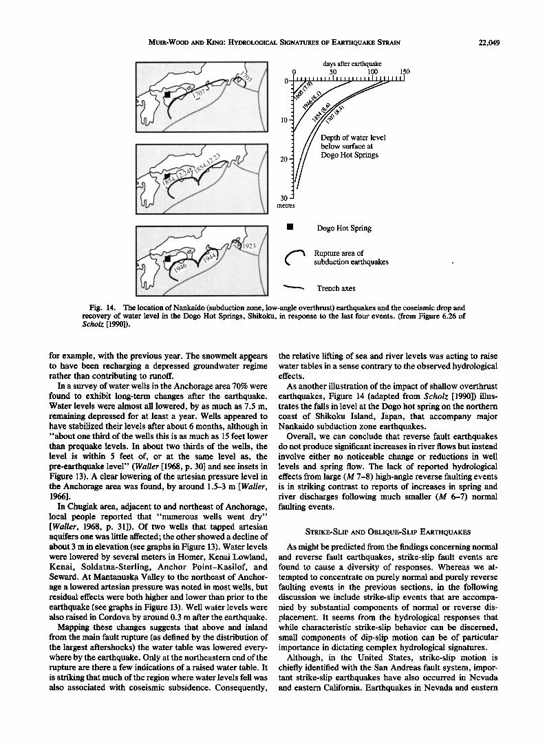
Fig. 14. The location ofNankaido (subduction zone, low-angle overthrust) earthquakes and the coseismic drop and recovery of water level in the Dogo Hot Springs, Shikoku, in response to the last four events. (from Figure 6.26 of Scholz [1990]).

for example, with the previous year. The snowmelt appears to have been recharging a depressed groundwater regime rather than contributing to runoff.

In a survey of water wells in the Anchorage area 70% were found to exhibit long-term changes after the earthquake. Water levels were almost all lowered, by as much as 7.5 m, remaining depressed for at least a year. Wells appeared to have stabilized their levels after about 6 months, although in "about one third of the wells this is as much as 15 feet lower

than prequake levels. In about two thirds of the wells, the level is within 5 feet of, or at the same level as, the pre-earthquake level" (Waller [1968, p. 30] and see insets in Figure 13). A clear lowering of the artesian pressure level in the Anchorage area was found, by around 1.5-3 m [Waller, 1966].

In Chugiak area, adjacent to and northeast of Anchorage, local people reported that "numerous wells went dry" [Waller, 1968, p. 31]). Of two wells that tapped artesian aquifers one was little affected; the other showed a decline of about 3 m in elevation (see graphs in Figure 13). Water levels were lowered by several meters in Homer, Kenai Lowland, Kenai, Soldatna-Sterling, Anchor Point-Kasilof, and Seward. At Mantanuska Valley to the northeast of Anchor- age a lowered artesian pressure was noted in most wells, but residual effects were both higher and lower than prior to the earthquake (see graphs in Figure 13). Well water levels were also raised in Cordova by around 0.3 m after the earthquake.

Mapping these changes suggests that above and inland from the main fault rupture (as defined by the distribution of the largest aftershocks) the water table was lowered everywhere by the earthquake. Only at the northeastern end of the rupture are there a few indications of a raised water table. It is striking that much of the region where water levels fell was also associated with coseismic subsidence. Consequently,

the relative lifting of sea and river levels was acting to raise water tables in a sense contrary to the observed hydrological effects.

As another illustration of the impact of shallow overthrust earthquakes, Figure 14 (adapted from Scholz [1990]) illus- trates the falls in level at the Dogo hot spring on the northern coast of Shikoku Island, Japan, that accompany major Nankaido subduction zone earthquakes.

Overall, we can conclude that reverse fault earthquakes do not produce significant increases in river flows but instead involve either no noticeable change or reductions in well levels and spring flow. The lack of reported hydrological effects from large (M 7-8) high-angle reverse faulting events is in striking contrast to reports of increases in spring and river discharges following much smaller (M 6-7) normal faulting events.

STRIKE-SLIP AND OBLIQUE-SLIP EARTHQUAKES

As might be predicted from the findings concerning normal and reverse fault earthquakes, strike-slip fault events are found to cause a diversity of responses. Whereas we attempted to concentrate on purely normal and purely reverse faulting events in the previous sections, in the following discussion we include strike-slip events that are accompanied by substantial components of normal or reverse displacement. It seems from the hydrological responses that while characteristic strike-slip behavior can be discerned, small components of dip-slip motion can be of particular importance in dictating complex hydrological signatures.

Although, in the United States, strike-slip motion is chiefly identified with the San Andreas fault system, important strike-slip earthquakes have also occurred in Nevada and eastern California. Earthquakes in Nevada and eastern



California reflect dextral strike-slip (generally N-S trending) faulting associated with normal motion. In the Transverse Ranges, sinistral strike-slip motion (E-W trending) associated with reverse motion occurs, and reverse dextral strike-slip displacement is also found associated with the San Andreas fault through the Santa Cruz Mountains south of San Francisco Bay. The range of strike-slip and oblique-slip earthquakes in this region has produced diverse hydrological signatures.

Of the normal strike-slip events the Cedar Mountain earthquake in Nevada on December 20, 1932, involved a broad zone of fault traces, trending generally N-S. Some springs and wells ceased flowing, others increased flow, and many were unaffected [Gianella and Callaghan, 1934]. On the same day south of the 1954 Dixie Valley normal fault displacement, there was movement on a N-S trending zone of normal strike-slip displacement passing through Fairview Valley. At the northern end of this zone, close to the junction with the Dixie Valley fault there was a diverse range of responses predominantly involving a fall in water level. Farther to the south along the fault zone, a well that was located close to the fault strands underwent an initial fall, followed by a rise that was higher than its original level [Zones, 1957]. The largest of the normal strike-slip earthquakes in this region occurred in the Owens Valley, eastern California, on March 26, 1872. Springs dried up along some sections of the fault, but along others many new springs were formed [Hobbs, 1910].

In the far southwestern part of California and over the border into Baja California there are a number of en echelon sections of NW-SE trending strike-slip faults, all involving dextral motion. The February 9, 1956, earthquake originated on the San Miguel fault and involved at least 15 km of surface rupture [Shor and Roberts, 1958]. At the northwestern end of the fault, warm water began to flow within a few hours of the earthquake at a rate estimated as 32-35 L/s. Two kilometers to the north at Rancho Agua Blanca, and on the other side of the projected line of the fault, springs went dry. An increase in flow was also noted at the Tres Campos springs to the west of Rancho Arroyo Grande along the projection of the fault to the southeast.

The San Andreas fault to the north of the Transverse

Ranges is involved in continuous creep. Water wells adjacent to the San Andreas fault have been monitored since the

early 1970s and have been found to respond to creep events along the fault [see Johnson et al., 1974; Roelofts et al., 1989]. The nature of the change, whether a rise or a fall, was identified by Johnson et al. as reflecting the location of the creep event relative to the wells.

In the great 1906 San Francisco earthquake, hydrological changes were noted scattered across northern California [Lawson, 1908]. The most significant changes involving new springs and increased stream flow were noted within the region from Napa to Gilroy on the eastern side of San Francisco Bay. Similar manifestations of increased stream flow were also noted down the San Francisco peninsula. Elsewhere, increases in flow tended to be modest and isolated. In the coastal region of northern Sonoma and Mendocino counties the majority of observations recorded decreases in flow and wells drying up after the earthquake.

There are two oblique-slip earthquakes in California for which quantitative information on the hydrological response is available, the M 7.2 Kern County earthquake of July 21, 1952, which involved reverse and sinistral strike-slip dis-

placement on the White Wolf fault [Buwalda and St. Amand, 1955] and the oblique reverse dextral strike-slip Loma Prieta M 7.1 earthquake of October 17, 1989.

Kern County Earthquake

A review of quantitative information on changes in stream flow across central California, following the July 21, 1952, earthquake is reported by Briggs and Troxell [ 1955], including river flow data that can be examined in the same way that we considered normal faulting events. Figure 15 shows a map of rivers with flow gauges identified as before together with locations of watersheds for which information is avail-

able. Flow information has been replotted, at 5-day intervals, in a series of graphs around a map of the watersheds. The peak increase in flow has been estimated for all streams for which gauged data are available by subtracting the flow immediately prior to the earthquake from the maximum flow in the following month (since there was some variation in the risetime to peak flow, from 5 to 20 days PE). A marked variation in the apparent duration of the hydrological response can be seen in the figures. At Grapevine Creek in the hanging wall of the White Wolf fault, excess flow cannot be traced for more than 30 days, while in Walker Basin Creek and Caliente Creek at the northeast end of the fault break, the decay is much slower and excess flow was still occurring the following summer. The longest of all decay times was for a few springs in the Santa Ynez Mountains to the north of Santa Barbara, where detailed hydrological observations were undertaken as part of the construction of the Tecolote Tunnel [Rantz, 1962]. The flow from one small spring (identified by Briggs and Troxell as the Canatsey-O'Bannon Spring from the names of two ranch owners living in its vicinity) on the south side of the Santa Ynez Mountains took more than 4 years to return to its original level.

From the estimated form of the decay curves, extrapolated where necessary from the 70-day record of postearth- quake data, cumulative excess flow has been assessed for all drainage basins for which information is available. The drainage basins both to the north and south of the Santa Ynez Mountains have been combined, and the cumulative flow for the whole mountain range has been estimated from all the stream and spring flow information published by Rantz [1962].

In Figure 16 the peak excess flow is plotted for the 1952 Kern County earthquake, and total excess flow is shown in Figure 17. In both cases these have been normalized over the area of individual drainage basins in terms of excess rainfall equivalents (millimeters per day for peak excess flow; millimeters for total excess flow). Although the coverage of suitably gauged catchments is not comprehensive, the available rivers provide a good sample in almost all azimuths.

Drainage basins that were subject to excess flow following the earthquake extend in an arc, oriented approximately along the line of the fault. The highest values of cumulative excess flow were found around the northeast end of the fault.

Discharge was concentrated in the hanging wall, about 20 km behind the surface trace of the fault. This is in marked

contrast to a comparable traverse through the drainage basins around a normal fault trace, such as those of Hebgen Lake and Borah Peak. Close to the fault itself, two springs went completely dry following the earthquake, and a third only recovered following a large aftershock a month later [Briggs and Troxell, 1955].


Fig. 16. Peak excess flow following the White Wolf fault earthquake of July 21, 1952, normalized for the area of individual drainage basins and expressed as rainfall equivalents (in millimeters per day). Darkest shading indicates a lack of information or catchments with less than a total of 0.01 mm/d excess flow. Those with greater flow have been shaded in three lighter tones corresponding to 0.01-0.2, 0.2-0.4, and >0.4 mm/d.

Loma Prieta Earthquake

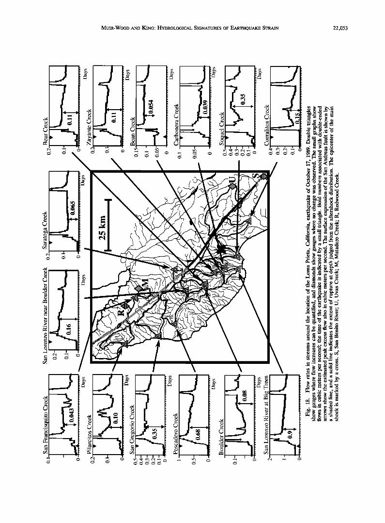
In a series of graphs on Figure 18, daily flows are plotted for all catchments around the Loma Prieta earthquake for which monitored river flows (from USGS Water Resources Data, California, Water Year 1990) showed an increase in discharge following the October 17, 1989, earthquake. River gauges immediately downstream from reservoirs have not been employed, but other catchments and river gauge locations are identified in Figure 18 for which there was no increase in flow following the earthquake.

Within a few days of the earthquake, on October 21 and 23, there were two rainfall events, whose characteristic, rapid runoff spikes overwhelm the postseismic increases in flow for a few days. However, flows rise to a plateau level that can be seen in almost all of the catchments illustrated.

As with the White Wolf fault earthquake there is some diversity in risetimes. Although for most gauges the peak excess flow has been calculated by subtracting flows 10 days PE from those on October 16, for two rivers which appear to have a longer risetimes, the peak flow has been determined

Fig. 17. Total excess flow following the White Wolf fault earthquake of July 21, 1952, normalized for the area of individual drainage basins and expressed as rainfall equivalents (in millimeters). Darkest shading indicates a lack of information or catchments with less than a total of 1 mm excess flow. Those with greater flow have been shaded in three lighter tones corresponding to 1-20, 20-40, and >40 mm.


I I I


Fig. 19. Peak excess flow following the Loma Prieta, California, earthquake of October 17, 1989, normalized for the area of individual drainage basins and expressed as rainfall equivalents (in millimeters per day). Darkest shading indicates a lack of information or catchments with less than a total of 0.01 mm/d excess flow. Those

with greater flow have been shaded in three lighter tones corresponding to 0.01-0.2, 0.2-0.4, and >0.4 mm/d.

15 days PE (Corralitos Creek) and 20 days PE (Soquel Creek). These increases are used (Figure 19) to estimate the values of peak excess flow normalized over the area of the individual catchments and expressed in terms of daily rainfall equivalents. Peak equivalent rainfall values have been banded in three shades consistent with those employed in other maps of peak excess discharge.

Peak excess discharges can be seen to range up to 0.85 mm/d in the headwaters of the San Lorenzo River, located at the northwestern end of the fault rupture. In the hanging wall of the fault rupture (on the southwestern side of the San Andreas fault), peak excess flows are found in all catchments. However, for those rivers draining to the northeast of the Santa Cruz Mountains only those whose headwaters lie to the southwest of the San Andreas fault (such as Saratoga Creek and San Francisquito Creek) showed a postseismic increase in discharge. Adjacent catchments such as those at Redwood Creek and Matadero Creek that lie entirely to the northeast of the San Andreas fault showed no increase in

flow. The Santa Cruz Mountains experienced a pronounced drought before and in the months following the Loma Prieta earthquake, and it is therefore relatively simple to follow the excess discharge throughout the winter of 1989-1990. For many of the smaller drainage basins there was no flow prior to the earthquake. Expected flow curves, where required, have been based on the previous year's flow when precipitation was similar. Hence decay times for all catchments can be explored directly.

In Figure 20 the total excess river flow has been plotted, normalized to the area of each individual drainage basin as total rainfall equivalent excess flow. Figure 20, which has the same shading intervals, may be compared with Figure 17 for the White Wolf fault earthquake (and also with Figures 5 and 8). In common with the White Wolf fault earthquake and in contrast to a normal fault earthquake, discharge is found

mainly in the hanging wall with concentrations at and beyond the fault ends. In both earthquakes, at a number of locations close to the projected surface trace of the faults, the water tables (as indicated by well levels) fell. The similarities between the hydrological signatures of these two Californian reverse/strike-slip earthquakes are prominent. Around the Santa Cruz Mountains, while many of the hanging wall catchments that showed an increase in flow have high topography, other footwall rivers that drain equally severe topography at similar epicentral distances showed no flow increases.

The cumulative excess discharge, found by summing the extrapolated excess flow information from all the drainage basins from the White Wolf fault and Loma Prieta oblique reverse-strikeslip earthquakes, was estimated to be 0.025 and 0.015 km 3, respectively. These values are smaller by more than an order of magnitude than the excess flow for the similar sized Hebgen Lake and Borah Peak normal fault earthquakes. Hence both the geographical distribution and the cumulative total of excess flow appear related to the style of faulting.

MODELING HYDROLOGICAL EFFECTS

Before discussing our favored view of the mechanisms that cause the diverse hydrological signatures of different styles of earthquakes it is appropriate to give a short review of some of the alternative models that have previously been proposed. First, the release of water is considered to reflect an increase in permeability of the near-surface rocks as a result of intense shaking [e.g., Rojstaczer and Wolf, 1992]. In such a model a correlation might be anticipated between

.... .-.:::ZZ:Z:iZiZZ. ß . ---.-:.v.-. •.•.,.•.

:-Xv.-. ..... '-.-.-.v. ;',..• :-'.'.:-'.{3} :-:-:-:-:-:-:-:-:-- .......

:::::::::::::::::::: , ,.•r., **

-:-.v:v.v.-. •.;.,¾;•. X-X-X-X-X-X-X-X- "'* .... •:,?•:.

Fig. 20. Total excess flow following the Loma Prieta, Califor- nia, earthquake of October 17, 1989, normalized for the area of individual drainage basins and expressed as rainfall equivalent (in millimeters). The surface expression of the San Andreas is shown by a shaded line, and a solid line indicates the extend of rupture at depth. The epicenter of the main shock is marked by a cross. Darkest shading indicates a lack of information or catchments with less than a total of 1 mm excess flow. Those with greater flow have been shaded in three lighter tomes corresponding to 1-20, 20-40, and >40 mm.


the level of ground shaking, or the proximity of fault rupture, to the size of the hydrological response. Some support for this view might be found in standard intensity scales in which changes in spring flow and well levels have sometimes become incorporated as an intensity indicator (intensity VIII on the 1931 Modified Mercalli Scale [Wood and Neumann, 1931]). However, this is probably a result of history: intensity scales were all first constructed in Italy and hence reflect experience primarily of normal fault earthquakes. Although for normal fault earthquakes perhaps, one could construct some simple relationship between the macroseismic intensity and the area over which water is released; for other fault styles there is no such relationship.

Rojstaczer and Wolf find support for their models for increased permeability from the fall of the level of some wells located on the ridge top immediately above the northwest end of the Loma Prieta fault rupture where nearby rivers increased in flow. While increased permeability might explain these observations, it cannot explain why mountain- ous catchments located on the other side of the San Andreas

fault were unaffected by flow increase. Permeability alone can also not explain how lowland well levels have been generally observed to fall in the region around reverse-fault displacements but rise in lowland regions similarly posi- tioned in relation to a normal fault earthquake. There is also no simple explanation for how an increase in permeability as a result of vibration, becomes reduced once again in the interseismic period. Hydrological signatures of different styles of fault movement, as reported in this paper, show no simple relation with either topography or earthquake size.

Sibson [1981, 1990] has developed "fluid pumping" and "fault valve" models. In the former, fault zone dilatancy collapses and expels water at the time of the event and will be discussed below together with other similar models, while in the latter the processes of the earthquake cycle increase porosity which is then exploited by upward passage of fluid driven by high pressures at depth. In this model, the fault is assumed to act as an impermeable seal between earthquakes but forms "highly permeable channelways for fluid flow immediately postfailure as a consequence of the fractal roughness of natural rupture surfaces" [Sibson, 1990, p. 1586]. Sibson [1990, p. 1588] suggests that "the most vigor- ous fault-valve activity is likely to occur in compressional tectonic regimes." Whatever the merits of seismic valving (in particular, as an explanation for mineralization around the brittle-ductile boundary), surface hydrological effects accompanying different styles of earthquakes cannot be explained by valving. Far more water is discharged after normal fault earthquakes than after reverse fault earthquakes. Even in the oblique reverse-strike-slip 1952 Kern County, White Wolf fault event (Figure 15-17), quoted by Sibson, much of the discharge was at considerable distances from the causative fault, while the closest springs to the fault went 'dry following the earthquake.

Dilatancy Model

Another potential model for changes in pore pressures, in association with fault rupture, is "dilatancy" in which prior to failure the rock expands as a result of the application of a high deviatoric stress [Brace et al., 1966]. In the dilatancy diffusion model [Scholz et al., 1973] increased opening of cracks due to very high levels of shear deformation is

assumed to lead to a phase of strain hardening as the hydraulic diffusion can no longer sustain the pore pressure. Eventually, when the pore pressure recovers, the rock is weakened and the fault rupture initiated. Hence the water table is predicted to become lowered before the earthquake with a phase of postseismic (and potentially immediately preseismic) water release.

A number of instances have been encountered in this, and other studies [e.g., Roelofts, 1988] of hydrological changes in advance of earthquakes that may be indicative of dilatancy. In particular, there are reports from several normal fault earthquakes of water levels dropping, and springs drying up in a period of weeks or months prior to an event (as, for example, the December 17, 1857, earthquake in southern Italy, Battista, 1858). These phenomena always appear to be concentrated close to the eventual fault rupture, suggesting that dilatancy is only locally significant. Where seen in well levels or spring flows, the size of these premonitory hydrological signals is small in comparison with the magnitude and geographical extent of the postseismic hydrological responses. While dilatancy collapse could explain some near- fault coseismic effects, it cannot explain more distant effects. Also a shear-induced dilatancy model cannot, on its own, explain the extreme disparity that exists between the hydrological signatures of normal and reverse fault earthquakes.

Coseismic Strain Model

The most satisfactory explanation for the hydrological signatures of different styles of fault displacement comes from models of coseismic strain. In most igneous, metamor- phic, and well-lithified sediments, typical of the upper crust, mobile water is held and transported in fractures and variations in stresses, and their consequent strain changes are well known from experimental laboratory studies to be accommodated by alterations in fracture aperture [Walsh, 1965; Batzle et al., 1980]. Hence it is to be anticipated that crustal strain will alter crustal porosity.

An early attempt to explain changes in well levels according to the regional strain field of a strike-slip earthquake in Japan was made by Wakita [1975]. However, no previous research has attempted to compare the predicted strain fields of normal and reverse fault earthquakes with their hydrological effects. However, such models can readily explain the difference between the hydrological signatures of normal and reverse fault earthquakes, the geographical extent of the hydrological response, and even, in general terms, the magnitude of the water release.

A schematic version of the model we envisage, in which strain associated with the earthquake cycle opens and closes preexisting fractures, is shown in Figure 21. For extensional faulting, the interseismic period (Figure 2 l a) is associated with crack opening and an increase of effective porosity. At the time of the earthquake (Figure 21 b), cracks close and water is expelled. For compressional faulting the reverse occurs; during the interseismic period (Figure 21c), cracks close expelling water. At the time of the earthquake (Figure 21 d), cracks open and water is drawn in. Such models are qualitatively consistent with our observations.

In order to examine in more detail the expected magnitude and extent of strain-induced hydrological effects, strain models of coseismic deformation have been generated using a boundary element program in which dislocation elements


NORMAL FAULTING

a•

Interseismic extension Coseismic compressional elastic rebound

REVERSE FAULTING

c)

Interseismic compression

_..

Coseismic extensional elastic rebound

Fig. 21. Simplified model for the interseismic accumulation and coseismic release of strain in extensional and compressional tectonic environments. (a) For extensional faulting, the interseismic period is associated with crack opening and increase of effective porosity. (b) At the time of the earthquake, cracks close and water is expelled. (c) For compressional faulting, the interseismic period is associated with crack closure and the expulsion of water. (d) At the time of the earthquake, cracks will open and water will be drawn in. In the case of normal faulting, water can be expelled on to the surface at the time of an earthquake and thus immediately affect river flow (shown schematically as surface fountains). For reverse faulting, cracks must be filled from the water table, a slower process that may not be observed in river flow rates. For clarity, only vertical cracks are shown. If preexisting cracks exist, opening and closure of vertical ones will be the predominant effect in changing porosity (see text and Figure 22).

are introduced into an elastic medium. Details of such

models are given by Bilham and King [1989] and King and Ellis [ 1990]. Figure 22 is an illustration of the dilational strain changes that accompany displacement on a 45 ø dipping normal fault, both in cross section (Figure 22a), plan view at the surface (Figure 22b) and plan view at a depth of 5 km (Figure 22c). Light shading represents a reduction of volume and dark areas represent dilation. (The convention is selected to be compatible with the earlier figures of peak or total water flow where excess flow was indicated by light shading, on the assumption that coseismic reduction of volume causes water to be expelled.) The predominant strain changes are compressional. However, some complexity of the strain field as a function of depth can be seen and results from the flexural component of deformation and the finite depth of faulting; dark dilational areas occur near the base of the fault and superficially in the hanging wall. The strains due to a 45 ø dipping reverse fault are the opposite sign of those due to a normal fault. Appropriate figures for reverse faults would therefore be the same as Figure 23 reversing the arrows on the fault and the light and dark shadings.

In Figure 24 the strain field is modeled surrounding a 45 ø dipping strike-slip fault. Unequal quadrants of negative and positive strain appear. For a vertical fault the size of the lobes on each side of the fault would be equal, the inequal- ities being due to fault dip. The addition of dip-slip motion or fault motion that does not reach the surface adds greater

,

complexity. Models that include both dip-slip and strike-slip motion appropriate to the geometry of the Kern County and the Loma Prieta earthquakes are shown in the next section.

COMPARISON OF HYDROLOGICAL SIGNATURES

WITH STRAIN MODELS

The observed regions of water discharge and compressional strain for the boundary element model in Figure 22c are in agreement for both the Borah Peak and Hebgen Lake earthquakes. It should be noted when comparing the figures that the surface fault breaks shown in Figures 3-5 and 6-8 are shorter by a factor of 2 (or more) than the faulting that aftershock and teleseismic data suggest is the true extent of faulting at depth. The narrow and shallow band of dilation (Figure 22c) is not observed in the cumulative hydrological effects (although risetimes may be affected), suggesting that water is expelled by volume changes over depths in excess of 1-2 km.

The White Wolf fault and Loma Prieta earthquakes involved oblique-slip displacement and are less straightfor- ward than the simple normal fault geometries. Nonetheless, models based on geodetic data adequately explain the observations. In Figure 24a near-surface strains (0.1 km depth) are shown based on the fault model for the Kern County earthquake derived by Stein and Thatcher [1981]. The compressional areas are consistent with the observed regions of water expulsion (Figures 15-17). Figure 24b shows the strain distribution for the same fault model for a depth of 5 km. This shows that the hanging wall compression is superficial, being absent at this depth. Consistent with this, an examination of Figure 15 shows that in the hanging wall the duration of flow and total amount of water expelled was much less than for the large compressional region at the


eastern end of the faulting where both strike-slip and dip-slip motion combine to produce compression over a wide depth range.

Figure 24c shows the volume strains at a depth of 2.5 km for the fault model of the Loma Prieta earthquake from Marshall et al. [1991]. Regions of volume compression are consistent with observed regions of water expulsion, although no data are available for the drainage basins to the

Strike-slip motion on a Dipping Fault

a) -60.00 - 30.00 0.0 30.00 60.00 0.0

20.00

Dip-slip motion on a Dipping Fault

a)

b)

-60.00 -30.00 0.0 30.00 60.00 0.0

km

20.00

-60.00 -60.00

-30.00

0.0

30.00

60.00

-30.00 0.0 30.00 60.00

Strains the •r• -. _. _- _•_ ]--.:::• Surface : - -_ ._.,...__: ........

-60.00 -30.00 0.0 30.00 60.00

C) -60.00

- 30.00

0.0

30.00

60.00 ..................

Fig. 22. (a) Cross section and (b) plan view of strains modeled at the surface and (c) at a depth of 5 km around a 45 ø dipping normal fault in a half-space. Strain levels are shaded from a background grey to lighter shades (negative strain) and to darker shades (positive strain) in strain steps of 2 x 10 -5. The strains for a reverse fault dipping at 45 ø have the same distribution and amplitude but opposite sign.

b) -60.00 -30.00 0.0 30.00 60.00 -60.00

-30.00

0.0

30.00

60.00

Fig. 23. (a) Cross section and (b) plan view of strains at the surface around a dipping strike-slip fault in a half-space. In Figure 23b, strain levels are shaded from a background grey to lighter shades (negative strain) and to darker shades (positive strain): strain steps of 2 x 10 -5.

southeast of the fault rupture where increased flow is predicted. The steeper dip and deeper burial of the faulting are responsible for the differences in form between the Loma Prieta and White Wolf fault models.

In the case of the Borah Peak and Hebgen Lake earthquakes the strain predicted from seismically and geodetically determined earthquake parameters, can be compared with the magnitude of the cumulative excess flows in more detail. In Figure 25, cumulative rainfall equivalent discharges along a traverse perpendicular to the strike of each of the faults are compared with those predicted for a two-dimensional strain model. The thicker lines are predictions based on the assumption that all of the volume strain (areal strain since linear strain in the third dimension is taken to be constant) to some specified depth is expressed as a change of porosity due to the closure of cracks of all orientations and that all of

the displaced water appears at the surface. It might be supposed that only vertical cracks dominate so that only horizontal linear strain is important. Thin lines in Figure 25 show the predicted flow for the 5-km depth range for this latter assumption. Since they are scarcely different from the assumption that areal strain is dominant, we conclude that we cannot tell whether anisotropy of crack orientation exists. Since the models are two-dimensional, implying an infinite fault length, they may be expected to overestimate the discharge at distances greater than the true fault length (about 40 km).


a) 0.0

0.0 50.00 100.0 150.0 200.0

50.00

100.0

150.0

b) 0.0 50.00 100.0 150.0 200.0 0.0

50.00

100.0

150.0

Fig. 24. Plan view models for the volume strains associated with the Kern County and Loma Prieta earthquakes. Strain levels for all figures are shaded from a back,ground grey to lighter shades (contractional strain) and to darker shades (extensional strain)' strain steps of 2 x 10 -•. (a) Surface strains and (b) Strains at 5 km depth are shown for fault parameters appropriate for the Kern County (White Wolf fault) earthquake for comparison with Figures 16 and 17. The compressional strains in the hanging wall only appear at shallow depths where the flow of expelled water (Figure 15) diminishes much more rapidly than where compressional strains extend to greater depth. (c) Compressional strains at a depth of 2.5 km for a fault with parameters appropriate for the Loma Prieta earthquake are shown. This should be compared with Figures 19 and 20. In all of the figures, outlines of the catchment areas for the corresponding earthquake epicentral region are shown.

For the Hebgen Lake earthquake the closest fit is with the 5-km depth prediction both in general shape and in amplitude. The fit is remarkably good, and the data are not very sensitive to where the profile is taken. For Borah Peak,

discharge in the catchment including the fault is likely to be underestimated as a result of the recharge of groundwater in the gravels of the broad Lost River valley. The fault also had a significant strike-slip component of displacement, which


c)

-30.00 0.0 30.00 -30.00

60.00

.0000

30.00

60.00

Fig. 24. (continued)

may explain why, in a profile through the southern part of the hanging wall, the flow is greater than predicted, although this peak is absent to the north.

Despite the limitations of the data, two conclusions are unavoidable. First, the water that appears at the surface is associated with fracture systems extending to considerable depth. Second, a large part of the coseismic volumetric strain causes the closure of cracks and expulsion of water. Either all of the earthquake volume strain is associated with crack closure down to about 5 km or fractures are connected

to greater depths and only part of the volume strain is associated with a reduction in porosity. However, depths much greater than 10 km seem improbable in view of other earthquake parameters; thus at least 50% of the volume strain must result in crack closure. It is important to appre- ciate that such large proportions of volume strain occurring as a reduction of porosity can only occur if the mobilized fluids are in high aspect ratio interconnected cracks. If fluids exist in low aspect pores, they will not be mobilized.

From the hydrological information collected at Borah Peak and around Hebgen Lake there is only limited evidence in support of any dilational strain effects (involving a drawdown in the water table) modeled at the ends of the fault rupture. Along the continuation of the Hebgen Lake fault toward the southeast, the Yellowstone Park geyser fields overlie the Yellowstone caldera. The seismogenic crust in this region is thin, but the response of the geysers to the earthquake suggests a diversity of shallow strain changes. For most models of geyser plumbing, the frequency of geyser eruption reflects the flow rate of the underlying superheated water column. While a number of geysers showed increased activity following the earthquake, others, including Old Faithful, declined in activity, with the period

between eruptions increasing. A number of aftershocks of the Hebgen Lake earthquake had epicenters within the geyser field and were associated with further alterations of eruptive activity [Marler, 1964].

In the Borah Peak earthquake, wells distributed along the prolongation of the line of the fault, between 150 and 200 km to the south, dropped in level at the time of the earthquake [Wood et al., 1985b], one of them returning back to normal following a large aftershock, suggesting again that the strain "shadow zone" was subsequently released through further faulting. However', indications of dilational strain were, as in the Hebgen Lake earthquake, far less widespread or significant than those suggested by coseismic strain models.

The only normal fault earthquake known to us for which there appears to be stronger evidence in support of more widespread strain shadows is the south Italian Baranello event of July 26, 1805 (see Figure 12), in which the distribution of springs either drying up or decreasing in flow looks remarkably similar to the strain shadows predicted by the strain model, to lie beyond the ends of the NW-SE trending normal fault. Strain shadows may also explain the observation for the 1896 Rikuu reverse fault earthquake, where in the hanging wall hot springs stopped or suffered reduced flow, while a new spring appeared at the end of the fault.

Causes of the Disparity Between the Hydrological Effects of Normal and Reverse Fault Earthquakes

In general, the release of water in the form of increased river or spring flows or raised well levels associated with normal fault earthquakes appears far more commonplace than the lowering of the water table or reductions of flow in response to reverse fault events. The most obvious explana-


45o; a) 400 •

350 •

300 •

200 ]

lOO•

Hebgen Lake

-50

-80 -60 -40 -20 0 20 40 60 80

250

b)

200

150

100. .

,50-

-50

-80

Borah Peak

10 kilometer

ß

ß -;o ' -;o no

Fig. 25. Observed and predicted total flow for cross sections perpendicular to the strike of the (a) Hebgen Lake and (b) Borah Peak earthquakes. Thicker solid lines are predicted from the areal strain summed to depth ranges of 2, 5, and 10 km and converted to effective total flow (in millimeters). The thinner lines are for the horizontal strain for the 5-km range converted to flow. The faults have a constant slip (6 m for Hebgen Lake and 3 m for Borah Peak) on a 45 ø fault extending to a depth of 15 km. In Figure 25b, observed values across the upper Lost River tributaries are shown as a thin stippled line, alongside a thicker stippled line taken farther to the west and interpolated around the fault where there was significant water loss in the broad Lost River Valley.

tion of the difference in river behavior is that expelled water can rapidly reach rivers by increases of spring flow, but a reduction of fluid pressure within the upper crust will not rapidly draw water from rivers. Other phenomena may also enhance the disparity. First, crustal permeabilities may tend to be higher in a region subject to extension than one involved in compressional deformation. Second, cracks close normal to the maximum compressive stress direction, with dilation of cracks oriented normal to the minimum

stress direction. In both normal and strike-slip tectonic environments, enhanced permeabilities will tend to be along vertical fractures, while in compressional tectonic environments, enhanced permeabilities are expected to lie in the horizontal plane.

These factors could conspire to limit the rate at which a positive strain change in a compressional tectonic environment can influence a surface water table. Clearly, if this rate

becomes so slow that the water table is affected only after several months, then a relation with the earthquake is unlikely to be recognized and the signal itself will be completely obscured by precipitation.

MODELING THE FORM OF HYDROLOGICAL SIGNATURES

The simplest model to describe the origin of the observed hydrological signatures is to assume that they result from flow in a series of planar uniform cracks open at the surface, closed at some depth and subject to a pressure change over a depth range that does not extend fully to the surface (Figure 26a). This depth over which pressure changes have no effect defines a dead depth. Below the dead depth the pressure effect on the crack is assumed to be constant to the closed base of the crack. The mathematics of the model are

described in the appendix. Figure 27 shows a series of flow versus time profiles both

as a function of crack width and the dead depth. Surface flow was found to be relatively insensitive in form to reasonable variations in pressure distribution below the dead depth. The crack width is the parameter most strongly controlling the decay of the flow versus time profile, while the dead depth and the crack width together determine the risetime. Most of the observations are fit by models in the center of Figure 27 with crack widths of about 0.03 mm and effective dead

depths of about 2 km. Typical examples of the fit of these theoretical models to observed profiles are shown in Figure 28 from the North Fork Big Lost River following the Borah Peak earthquake, the Galatin and Gardiner rivers following the Hebgen Lake earthquake, and Caposele Spring following the Irpinia earthquake.

The simple crack model can be interpreted in a general way. The decay time is determined by the fluid conductivity of the part of the system that responds to the pressure change, and the risetime is determined by the fluid conductivity of the system that connects the latter to the surface, the effective dead depth. The latter, in fact, includes the time constants of river flow or of surface aquifers and need not be associated with processes occurring at any great depth. It should therefore not be assumed that it truly represents a depth above which pressure changes do not affect flow. This is certainly the case for Irpinia with a 9-km dead depth (Figures 28) where we have already noted that the spring flow comes from an aquifer with a long flow time constant.

The fluid conductivity of the system that responds to pressure can also be interpreted differently. For example, models that assume Darcy rather than fracture flow could also produce the observed profile shapes. These are ex- cluded, however, because high aspect ratio cracks are required to expel large volumes of water from a rock body subjected to small strains. The same graphs as those shown in Figure 27 could also be created by cracks of the more convoluted form shown in Figure 26c, but unless the fluid paths are much longer, the crack widths required to give the same flow forms will only be slightly increased. Similarly, cracks could be made much shorter. Cracks of 1/8th the

length and 1/2 the width would have the same response (scaling relations may be seen by examining the equations in the appendix). However, to reach deep into the crust, the crack widths cannot be greatly reduced unless they are connected to the surface by high conductivity feeders (Fig- ure 26d). Fractal fissure systems such as those shown


a) Before crack closure

c)

h - Depth to which cracks extend

e- Crack width

w - Crack separation

b) After crack closure

d)

R - Rainfall equivalent

Wmax = h e Wmax - Crack separation if R cracks close completely

e)

Fig. 26. Equivalent cracks. Simple vertical cracks are shown (a) open and (b) closed. The equation indicates the crack separation w that can produce equivalent rainfall R for cracks of width e and depth h for the simple crack system. (c) A more convoluted crack system. Should the flow be very convoluted, the cracks will have to be slightly wider, but because of the e 3 term this is a small effect. (d) Short cracks with the same response as the cracks in Figure 26a are shown connected to a high conductivity channel, and (e) a fractal system is shown that is equivalent to the system in Figure 26a.

schematically in Figure 26e could have the same response as simple cracks and could plausibly drain appropriate depth ranges of the crust. In this model a crack of width e and length h connects to four cracks of width e/2 and length h/2. Each of these in turn connect to four cracks of width e/4 and

h/4 etc. To reach to depths of 5-10 km the largest of these cracks must again have widths of about 0.03 mm.

The information about crack widths and earlier estimates

of total volumes of water expelled and source depths allow us to estimate crack separations. As noted for a number of earthquakes, water expelled from fractures between the surface and 5 or 10 km deep in the crust can produce a maximum rainfall equivalent discharge in excess of 50 mm. Using the expression in Figure 26b for uniform vertical cracks and assuming that the cracks close completely this suggests separations of less than 3-6 m. In practice, it is improbable that cracks close by more than 50%, suggesting separations less than 1.5-3.0 m for uniform vertical cracks. Any of the more complicated systems shown in Figure 26a must have more cracks than the simple system of vertical cracks. We can therefore conclude that for regions of maximum water expulsion for the Hebgen Lake and Borah Peak active regions the brittle crust contains cracks of 0.03

mm or smaller with separations that cannot be much greater than 1 or 2 m. Even at distances from the epicenters of more than 50 km crack separations must be less than 10 or 20 m. These parameters can also be expressed as an equivalent hydraulic conductivity of a uniform porous medium [Mars- ily, 1986] and give values between 3.0 x 10 -9 and 5.0 x 10 -8 m 3 S -1 '

The similarity that exists among the hydrological signatures both close to and distant from that causative fault

suggests that the populations of fractures are not significantly affected by proximity to the active fault. Further- more, a variety of earthquakes have similar hydrological signatures, suggesting that such crack distributions are relatively ubiquitous.

HYDROLOGICAL SIGNALS OF SMALL EARTHQUAKES

The significant hydrological impacts of large earthquakes suggest that even small events should modify hydrogeolog- ical conditions. An estimate of the effect can be made. The

seismic moment distribution of earthquakes displays a power law type distribution typical of fractal sets [e.g., Aki, 1981; King, 1983] such that the volume of crust strained


Flow

mm/sec lkm

O. 10 0.05 0.00 ...... •" .... •.

O. 1()

0.05 o.oo ... 7'• •'.

().1()

().05

().0()

0.10

().()5

().1()

().()5

() 2 4

Depth from surface

1.5km 2km 3km 4km

Crack

width

•-•,.,,•.•.• ........ 0.05mm .

O.04mm

O.03mm

O.02mm

6 () 2 4 5[ •, d Months

0.01mm

Fig. 27. A range of predicted flows as a function of effective dead depth and crack width for the model described 10 1

in the appendix. Other parameters used are compressibility of water of 5.0 x 10- Pa- , viscosity of water of 1.0 x 3 8 1

10 Pa s, and effective compressibility of crack of 5.0 x 10- Pa- . The effective compressibility of the crack is chosen to be 100 times a typical unfractured rock compressibility. Note that since the crack width e appears in the expression for hydraulic conductivity as the cube and all other parameters affect the hydraulic conductivity in a linear or an inverse linear fashion, only very substantial changes in their values would affect the conclusions reached about crack width.

above some level can be obtained simply by comparing the moment of a small earthquake with that of a larger one whose hydrological field has been mapped in detail. Follow- ing the Hebgen Lake earthquake, total excess flow exceeded 20 mm over an area of 11,000 km2. Averaged over the top 5 km of the crust, this represents a strain of 4. x 10-6; over the top 10 km of the crust a strain of 2. x 10 -6. The volume of the rock mass subject to these strains correspondingly varies from 5 x 10 4 to 10 5 km 3. A magnitude 5 earthquake with a moment between 100 and 500 times less than the

Hebgen Lake event would create strains of about 3. x 10 -6 in a volume between 10 2 km 3 and 103 km 3 of crust. This is not too small to be observed.

As an illustration of the hydrological response of a small earthquake, the April 22, 1884, shock at Colchester, eastern England, had a magnitude assessed (from felt areas) to be Ms 4.4, and from regional neotectonic indications it is likely to have involved a significant component of normal fault displacement. From the macroseismic effects the event must have been shallow, occurring in the crystalline basement below a relatively thin cover of chalk. Following the earthquake the water table rose by more than 2 m over an area in excess of 100 km 2 [Meldola and White, 1885]. The detailed records of one well, located about 25 km from the epicenter, are shown in Figure 29. The slow decline in levels back to those prior to the earthquake bears a close resemblance to records of spring and river flows obtained from earthquakes with more than a thousand times the energy release. Signif- icantly, this earthquake occurred in an area with very gentle topography not exceeding 50 m. Thus the rise in well water

levels cannot be attributed to the draining of higher topography.

NEAR-FAULT STRAIN

Close to a fault, high levels of strain can be localized where there is a change in the displacement vector, a change in orientation of the fault, or a change in the plane of the displacement. According to the nature of the change in the fault displacement vector or fault plane the resultant strains can be either dilatational or compressional [Carrigan et al., 1991]. Furthermore, levels of strain in the immediate vicinity of a fault can rise much higher than those we have so far discussed in the regional strain field (<10-5). For example, if a fault jog reflects a jump in the plane of a fault by 100 m, and the fault displacement is 1 m, then horizontal strains as high as 10 -2 must be accommodated.

The sign of the strain change in the vicinity of a fault can also be independent of the regional strain field. Hence observations from springs and wells in the immediate vicinity of the fault may not be typical of the regional response: for example, a spring may dry up on a dilatational fault jog along a normal fault and water levels rise or spring flows increase from a compressional fault jog along a reverse fault. Such near-fault hydrological effects are not uncommon. Unlike the hydrological effects that we have described, local fault effects are characterized by their rapid onset. For vertical strike-slip faults, such hydrological signatures are seen only along the fault trace itself, but for dip-slip faults, concentrations of strain at a depth of a few kilometers seem


a] North Fork Big Lost River I al Hebgen Gardiner ) (Hebgen Lake)

,

m3s-1 m3s-1

I • 2km I I 2km

1• I = 0.03mm 0..• .... ! .... ! .... ! .... ! .... ! .... o

0 50 1 O0 150 200 250 300 0 50 1 O0 150 200 250 300

days PE. days PE.

"T^ ...... -T 'T .... Galatin River Caposele Spring

'i l[ ;X. Hebgen Lake) f ia) m3s-1 41 •'• •

t5 II X 1.5km / m3s. ]

ill • • 9km

0 0 50 100 150 200 250 300 0 50 100 150 200 250 300

days PE. days PE.

Fig. 28. Observed (solid line) and predicted (stippled line) flows for example discharges from Hebgen Lake, Borah Peak, and Irpinia earthquakes. Parameters used are the same as those quoted in the caption to Figure 27.

to find direct routes to the surface and can affect springs and wells in the hanging wall even at some distance (at least up to 5 km) from the fault trace. Hydrological examples of fault-related strain concentration were found on several

springs located in the hanging-wall of the Lost River fault, following the 1983 Borah Peak earthquake.

1.6 Messrs S. Courtauld's Well, Bocking

metres

1.4

1.2

1.0

0.8

0.6

0.4 [••"•.,,•: 1883 level 0.2 i i•1 i i i i i i i I i i i i i i i i 1884 1885

Fig. 29. Well levels at Bocking, near Braintree, Essex, before and after the Colchester earthquake of April 22, 1884. The well level was measured at weekly intervals. The levels for the months before and after April of the previous year are also shown.

DISCUSSION

In this paper we argue that coseismic hydrological effects can be clearly related to earthquake mechanism and involve substantial portions of the brittle crust. This has immediate consequences for our understanding of earthquake processes and of more general crustal mechanics. For example, the very low apparent flexural rigidities of the crust found by a number of workers [e.g., Ellis and King, 1991] become unsurprising in the presence of such fracture densities. The possibility of using carefully selected springs or wells as sensitive indicators of precursory earthquake strain is also placed on a sound basis if there is good reason to believe a direct fluid connection to the depths at which earthquakes initiate. The further idea that preseismic and postseismic changes of magnetic fields, or telluric currents, may be related to fluid flow (or the indirect electrochemical effects of fluid flow [Morat and Le Mouel, 1992]) also seems reasonable if we know we have connected fluid paths throughout the seismogenic crust. Our conclusions also carry important implications for a number of other disciplines in Earth Science.

Deep Hydrological Effects

Until now the only direct means to explore the depth to which fluid-filled cracks are interconnected has come from

deep boreholes and observations of certain types of reservoir induced seismicity. Postseismic water release offers a new and more powerful means to investigate flow to depth.


Earthquake water release may be thought of as a large-scale "well drawdown" experiment [e.g., Marsily, 1986] in which a conventional pressure reduction achieved by pumping at a wellhead is replaced by a uniform increase of pressure at depth. Actual drawdown experiments, however, never reli- ably measure deep permeability because they are masked by higher near-surface permeabilities; a problem alleviated if the pressure change is applied within the crust.

Temporal Changes in Seismic Velocities and Changes of Earthquake Coda Q

Indirect methods of inferring the existence of fluid-filled microfractures have included measurements of shear wave

splitting to determine anisotropy [e.g., Crampin, 1987], and studies of the variation of P or S wave velocities or Q, in response to presumed stress-induced changes in crack aper- tures. For example, local reductions in P wave velocities and Q values have been found throughout the zone of microseismic activity that defines the assumed seismogenic reverse and reverse strike-slip New Madrid faults, in Mis- souri, site of the great 1811-1812 earthquakes. Reductions in the velocity of >7% in the top 5 km and >4% between 5 and 24 km depth along the main presumed fault structure have been reported [Al Shukri and Mitchell, 1988]. Recent studies of changes of coda throughout seismic cycles also assume that fluid-filled microcracks change aspect ratio as the seismic cycle proceeds [Aki, 1985].

Mineralization and Sedimentary Basin Hydraulics

The existence of a dense interconnected system of fluid- filled microcracks in the brittle crust has implications for mineralization processes, allowing water to come into contact with very large volumes of rock, thereby leaching and concentrating significant quantities of trace elements. In regions of active tectonics, seismic strain cycling can move fluids to conditions of lower pressure and temperature, thereby encouraging precipitation. Strain cycling in compressional and extensional regions may be expected to promote different styles of mineralization. Reverse faults draw water in at the time of an earthquake, while normal faults expel water. In the interseismic period, fluid is squeezed out of the crust in compressional tectonic environments but drawn into the crust in extensional regimes. Repeated episodes of precipitation as cracks have opened and closed through many episodes of the seismic cycle are a common feature of mineralized veins [e.g., Ramsay, 1980]. It is evident from our results here that whether or not

permanent traces can be found in the rocks, this opening and closing of fluid-filled interconnected joints is a widespread feature of the brittle crust and need not be hypothesized as peculiar to a particular mineralized region.

Most of the observations reported in this paper apply to regions in which there is continuity between water stored in fractured crustal rocks and surface-discharging aquifers. However, over a significant proportion of the continents and, in particular, the continental shelves, there are extensive sedimentary cover sequences of very low permeability that prevent, at least in the short-term, any connection between basement fluid pressures and near-surface aquifers. Many such areas have been studied in considerable detail as the existence of an impermeable sedimentary cover forma-

tion is a prerequisite for a hydrocarbon reservoir. In such environments, if pore pressure changes cannot be relieved through flow or recharge from the surface, then fluid flow resulting from interseismic and coseismic strain changes will be lateral, either within the fractured crust or within some overlying aquifer or aquifers near the base of the sedimentary cover.

The interaction of the contraction and dilation of fissures

associated with the different seismic cycles of reverse, normal, and strike-slip events may create conditions that assist in concentrating hydrocarbons from their source rocks and pumping them to potential reservoir formations. Follow- ing normal fault displacement fluids will tend to migrate away from the vicinity of the fault. The volumes of displaced fluid can be predicted to be comparable to those found emerging at the surface where there is no impermeable cover (i.e., 0.5 km 3 of fluid migrating laterally from a region 10,000 km 2, in area). The flux on the margins of such an area entirely covered by an impermeable overburden would be more than 1000 m 3 of fluid for every meter length of perimeter; in a 10-m-thick aquifer with a 10% dynamic porosity, fluid would move 1 km. Such pulsed episodes of fluid flow are likely to have a significant impact on the migration of hydrocarbons, in particular, when tectonic activity is resumed fairly late in the evolution of the sedimentary basin. Following a reverse fault displacement, fluid flow will be drawn toward the fault. In a large basin undergoing significant rifting or subsequent compressional deformation, these pulses of flow may determine the long- term distribution of fluids. An understanding of potential hydrocarbon migration paths requires an investigation of the strain cycling that has accompanied the tectonic development of a particular basin. Strain changes associated with earthquakes even thousands of years ago could explain the development of certain zones of overpressurization and underpressurization.

CONCLUSIONS

Reports of the hydrological effects of earthquakes have existed for more than 2000 years, but rather little sense has previously been made of the observations. In this paper we show that many features of observed phenomena can be simply explained where the mechanics of an earthquak ex•s known. In particular, the hydrological effect is related to the earthquake's focal mechanism. Events that involve a significant normal faulting component expel substantial quantities of water, whereas reverse faulting events do not. Strike-slip events typically also expel water in more restricted regions but not in the quantities associated with normal faulting events.

The amount of water expelled by a normal faulting event can be very large, and for the Hebgen Lake and Borah Peak earthquakes was 0.3 and 0.5 km 3, respectively. The predicted volume strain associated with these events can be

compared with the total amount of water expelled and requires that nearly all of the seismic volume strain is accommodated by fissure closure and fluid expulsion. A well-connected fissure system extending throughout much of the brittle crust must exist to permit the water to escape. The flow following an earthquake persists for several months, and the form of typical flow curves together with a knowl- edge that much of the brittle crust is involved allows an


estimate of maximum crack widths and maximum spacing to be estimated. Crack widths are typically about 0.03 mm. In the epicentral region, fault spacings cannot exceed 1 or 2 m, while even in regions within one or two fault lengths of the causative faults, spacings must be less than 20 m.

A multiply fractured brittle crust with closely spaced interconnected fluid channels has implications for many branches of earth science.

APPENDIX:

FLUID FLOW IN A PRESSURIZED CRACK

In this paper we attribute excess river flow to be the result of water expelled from porous rock as a result of stress due to an earthquake. Although a complete description of the problem would consider the coupling between the solid and the fluid, the errors involved in treating the two separately are small [e.g., Carrigan et al., 1991]. The stress conditions set up by the seismic event are first calculated, and these are then used as boundary conditions to determine the fluid flow. The nature of the porosity due to fractures can then be considered by converting uniform porosity to the equivalent behavior of a system of cracks [e.g., Marsily, 1986] and allowance for a preferred crack orientation by incorporating anisotropic permeability [e.g., Carrigan et al., 1991].

Since we argue that the mobilized porosity must exist as high aspect ratio cracks, this appendix directly considers the effect of a stress change on the flow in a crack. What this may lose in generality is gained by making our approximations clear and our numerical calculations so simple that errors are easily avoided.

We discuss only vertical cracks (Figure A1) for two reasons. First, stress changes that we consider are mainly horizontal and only effect vertical cracks in an important way. The data we consider cannot resolve small-scale processes near faults where other stress components become important. Second, at the large scales that we consider (much larger than those considered by Carrigan et al. [1991]), vertical flow to Earth's surface and not lateral flow will dominate. Thus we can treat the problem as being spatially one-dimensional. With these approximations the parameters involved become the change in effective pressure in the crack (which is equal to the change in horizontal stress at the time of the earthquake), the fluid conductivity of the crack (which depends on crack width), viscosity, and the elastic modulii of the rock and water. Although the modulus of water is lower than rock, the effect of the aspect ratio of the crack (defined below) is to cause the rock to act as if it had an even lower effective modulus. It is this lower modu-

lus that dominates the system as shown schematically in Figure Alc.

In Figure A1 the crack is part of a system that is regarded as continuously connected, such that prior to perturbation by an earthquake, the pressure is hydrostatic P0 = hpt7 (where p is density, h is the depth from the water table, and t7 is the acceleration due to gravity). The potential (head) is P = P - P0 the difference between the actual pressure in the crack and hydrostatic pressure. It is nonzero values ofp that cause fluid flow.

The fluid conductivity of the crack is

K = e3/12/z (A1)

where/z is the dynamic viscosity. The effective crack width for fluid flow is e. Throughout this calculation, we assume

a

Fig. AI. Modeling an irregular crack. (a) A crack with irregular walls. The extent in the z direction is L and in the y direction is W. Crack thickness is e and an "average" crack thickness appropriate for calculating fluid conductivity is e 0. (b) The irregular form of the crack is approximated by a series of ellipses since their response to imposed stress is well known. (c) Overall the system acts as shown schematically. The crack varies in width (an amount assumed to be small relative to e0) with a stress distance relation that depends on both the modulus of the fluid and the effective modulus of the crack. For highly elliptical cracks this modulus is very much less than either the rock or the fluid modulus.

that changes in crack width resulting from changes in pressure are sufficiently small that K may be considered to be constant. If the faces of the crack were exactly planar, the stress normal to the crack •rxx would equal P. The crack is not open everywhere but is closed in some places due to roughness as shown in Figure Ala. Thus the o'xx stress distant from the crack and P are not the same.

A convenient method of mechanically approximating a partially closed crack is to regard it as composed of a series of elliptical inclusions. The separation between the points of contact in the real crack is approximately the same as the long axes of the ellipsoids. This is shown in Figure Alb.

The relation between a small change of crack width/ie of an elliptical crack of length I and a change of pressure inside the crack/iP and the distant stress component normal to the crack •r•x is

/Se (/SP- 15o-•x) --=/3 (A2)

I E

(modified from Jaeger and Cook [1979]), where /Se is a separation of the crack faces for positive /iP. In (A2), E is Young's modulus and/3 is a geometric factor that is close to unity and is not included in later expressions.

From (A2) the relation between the rate of change of crack width as a result of a change of p (note that/Sp = /SP) for constant distant stress can be written

de/dp = eoH/E. (A3)

Here I in (A2) is replaced by e0H. H is the aspect ratio of the ellipse and is approximately the separation between contact


points in the real fissure divided by the mean width of the fissure.

The volume of a part of the fissure of length L in the z direction and W in the y direction can be written

de

V = eoL W + L W •p p. (A4) From (A3) and (A4),

P V - eoL W - eoL WH - (AS)

E

A volume of crack v per unit distance in the y and z directions is therefore given by

(A6)

and the mass of this volume of fluid is

M = vp(P)

= v[po- po(p/G)] (A7)

where p(P) is the density of the crack fluid at pressure P. At the reference pressure P0 the density is P0 and G is the bulk modulus of fluid.

From (A6) and (A7) the mass of fluid per unit length of crack can be written

M = e[1 - H(p/E)][p o - po(p/G)].

This can be written

M=eoPo[1-(•t-•)P+(•G)P2J and since

(A8)

(A9)

except for extremely large H then

Hence

(A10)

(All)

dM

(A12)

The flux in the z direction at any point in the crack is given by

Q = -Ke dz' where K is the fluid conductivity. Hence using the expression for mass balance at any point in the crack

dM/dt = dQ/dz,

we can write an expression for the rate of change of volume with time at any point in the crack:

Fig. A2. Summary of boundary conditions used to calculate flow from vertical cracks.

dt = •zz -Ke •z (A13) and, consequently, using (A12), the change of pressure with time is

dp dp dM dt dM dt

K d2p

Po +

(A14)

This can be recognized as the diffusion equation and can be solved using appropriate initial conditions.

At the surface, free flow is permitted; thus p = 0 and at the bottom of the crack, no flow occurs; thus dp/dz = 0. At t = 0 a distant stress change &rxx occurs. Equation (A2) shows that this can be represented by a change of p (equals a change of P). Thus an equivalent change of head p as a function of depth within the crack is applied.

The profiles studied in this paper could all be adequately fit by a profile that had no pressure change to a depth D and a constant change from there to the base of the crack. These conditions are summarized in Figure A2.

The series of problems in the text were solved by finite differences with the flow at the surface being calculated as a function of time.

Acknowledgments. The initial work for this project was undertaken as part of a project for HMIP, UK Department of the Environment. This work may be used in the formulation of UK Government Policy but at this stage does not necessarily represent UK Government Policy. Grateful acknowledgment is given to Brian Thomson for supporting this research. Funding was also provided to G. King by CNRS through INSU 92.3820 92.ATP.631. Critical reviews that have substantially improved our presentation have been provided by Gordon Woo, Pascal Bernard, Ghislain de Mars- ily, and Charles Carrigan.


REFERENCES

Aguilera, J. G., The Sonora earthquake of 1887, Bull. Seismol. Soc. Am., 10, 31-44, 1920.

Aki, K., A probabilistic synthesis of precursory phenomena, in Earthquake Prediction: An International Review, Maurice Ewing Ser., vol. 4, edited by D. W. Simpson and P. G. Richards, pp. 566-574, AGU, Washington, D.C., 1981.

Aki, K., Theory of earthquake prediction with special references to monitoring of the quality factor of lithosphere by coda method, Earthquake Predict. Res., 3, 219-230, 1985.

AI Shukri, H. J., and B. J. Mitchell, Reduced seismic velocities in the source zone of New Madrid earthquakes, Bull. Seismol. Soc. Am., 78, 1491-1499, 1988.

Ambraseys, N. N., and C. P. Melville, A History of Persian Earthquakes, 219 pp., Cambridge University Press, New York, 1982.

Ambraseys, N., and J. Vogt, Material for the investigation of the seismicity of the region of Algiers, Eur. Earthquake Eng., 3, 16-29, 1988.

Battista, R., 'II terremoto di Basilicate, Relazione, Potenza, Italy, 1858.

Batzle, M. L., G. Simmons, and R. W. Siegfried, Microcrack closure in rocks under stress: Direct observation, J. Geophys. Res., 85, 7072-7090, 1980.

Bell, J. W., and T. Katzer, Timing of late Quaternary faulting in the 1954 Dixie Valley earthquake area, central Nevada, Geology, 18, 622-625, 1990.

Bilham, R. G., and G. C. P. King, The morphology of strike-slip faults: Examples from the San Andreas, California, J. Geophys. Res., 94, 10,204-10,216, 1989.

Bowman, J. R., G. Gibson, and T. Jones, Aftershocks of the 1988 January 22 Tennant Creek, Australia intraplate earthquakes: Evidence for a complex thrust-fault geometry, Geophys. J. Int., 100, 87-97, 1990.

Brace, W. F., B. W. Paulding, and C. H. Scholz, Dilatancy in the fracture of crystalline rocks, J. Geophys. Res., 71, 3939-3953, 1966.

Briggs, R. C., and H. C. Troxell, Effect of Arvin-Tehachapi earthquake on spring and stream flow, in Earthquakes in Kern County, California During 1952, Bull. Calif. Div. Mines, 171, 81-98, 1955.

Bull, W. A., and P. A. Pearthree, Frequency and size of Quaternary surface ruptures of the Pitaycachi fault, northeastern Sonora, Mexico, Bull. Seismol. Soc. Am., 78, 956-978, 1988.

Buwalda, J.P., and P. St. Amand, Geological effects of the Arvin-Tehachapi earthquake, in Earthquakes in Kern County California During 1952, Bull. Calif. Div. Mines, 171, 41-56, 1955.

Byerley, P., The June 27 1925 Helena, Montana earthquake, Bull. Seismol. Soc. Am., 16, 209-265, 1926.

Carrigan, C. R., G. C. P. King, G. E. Barr, and N. E. Bixler, Potential for water-table excursions induced by seismic events at Yucca Mountain, Nevada, Geology, 19, 1157-1160, 1991.

Celico, P., Relazioni tra idrodinamica sotteranea e terremoti in Irpinia (Campania), Rend. Soc. Geol. It., 4, 103-108, 1981.

Cotecchia, V., and A. Salvemini, Correlazione fra eventi sismici e variazioni di portata alle sorgenti di Caposele e Cassano Irpinio, con particolare riferimento al sisma del 23 novembre 1980, Geol. Appl. Idrogeol., 16, 167-191, 1981.

Crampin, S., Geological and industrial applications of extensive- dilatancy anisotropy, Nature, 328, 491-496, 1987.

de Dolomieu, D., Memoire sur les tremblements de terre de la Calabre Ulterieure pendant l'annee 1783, 1784.

Dunn, J. A., J. B. Auden, A.M. N. Ghosh, and D. N. Wadia, The Bihar-Nepal earthquake of 1934, Mem. Geol. Surv. India, 73, 1-391, 1939.

Ellis, M., and G. C. P. King, Structural control of flank volcanism in continental rifts, Science, 254, 839-842, 1991.

Esposito, E., G. Luongo, A. Marturano, and S. Porfido, II terremoto di S. Anna del 26 Luglio 1805, Mem. Soc. Geol. Ital., 37, 171-191, 1987.

Gianella, V. P., and E. Callaghan, The Cedar Mountain, Nevada, earthquake of December 20, 1932, Bull. Seismol. Soc. Am., 24, 345-384, 1934.

Gordon, F. R., Water-level changes preceding the Meckering, Western Australia, earthquake of October 14, 1968, Bull. Seismol. Soc. Am., 60, 1739-1740, 1970.

Gregson, P. J., R. S. Smith, and K. F. McCue, An explanation of

water level changes preceding the Meckering earthquake of October 14, 1968, Bull. Seismol. Soc. Am., 66, 631-632, 1976.

Hobbs, W. H., The earthquake of 1872 in the Owen's Valley, California, Gerlands Beitr. Geophys., 10, 352-384, 1910.

Housner, G. W., The mechanism of sandblows, Bull. Seismol. Soc. Am., 48, 155-161, 1958.

Jaeger, J. C., and N. G. W. Cook, Fundamentals of Rock Mechan- ics, Chapman and Hall, London, 1979.

Johnson, A. G., R. L. Kovach, and A. Nur, Fluid-pressure variations and fault creep in central California, Tectonophysics, 23, 257-266, 1974.

Jones, C., The Pleasant Valley, Nevada, earthquake of October 2, 1915, Bull. Seismol. Soc. Am., 5, 190-205, 1915.

King, G. C. P., The accommodation of strain in the upper lithosphere of the earth by self-similar fault systems: The geometrical origin of b-value, Pure Appl. Geophys., 121,761-815, 1983.

King, G. C. P., and M. Ellis, The origin of large local uplift in extensional regions, Nature, 348, 689-692, 1990.

Lawson, A. C., The Californian earthquake of April 18, 1906, Rep. State Earthquake Invest. Comm. 1, Carnegie Inst. of Washington, D. C., 1908.

MacDonald, B., Remarks on the Sonora earthquake--Its behavior at Tepic, Sonora, etc., Bull. Seismol. Soc. Am., 8, 64-78, 1918.

Mallet, R., Great Neapolitan Earthquakes of 1857: The First Prin- ciples of Observational Seismology, 2 vols., Chapman and Hall, London, 1862.

Marler, G. D., Effect of the Hebgen Lake earthquake of August 17, 1959, on the hot springs of the Firehole Geyser Basins, Yellow- stone National Park, U.S. Geol. Surv. Prof. Pap., 435-Q, 185- 197, 1964.

Marsily, G. de, Quantitative Hydrogeology, Academic, San Diego, Calif., 1986.

Marshall, G. A., R. S. Stein, and W. Thatcher, Faulting geometry and slip from coseismic elevation changes: The 18 October 1989, Loma Prieta, California, earthquake, Bull. Seismol. Soc. Am., 81, 1660-1693, 1991.

Marturano, A., E. Esposito, S. Porfido, and G. Luongo, Important earthquakes in Southern Apennines, Italy, in Proceedings of Workshop on Historical Seismicity of the Central Mediterranean Region, edited by C. Margottini and L. Serva, pp. 151-164, Italian Commission for Nuclear and Alternative Energy Sources, Rome, 1987.

Matsuda, T., H. Yamazaki, T. Nakata, and T. Imaizumi, The surface faults associated with the Rikuu earthquake of 1896, Bull. Earthquake Res. Inst. Univ. Tokyo, 55,795-855, 1980.

Meldola, R., and W. White, Report on the East Anglian earthquake of April 22nd, 1884, Essex Field Club Spec. Mem., Macmillan, New York, 1885.

Morat, P., and J.-L. Le Mou•l, Signaux 61ectriques engendr6s par des variations de contrainte dans des roches poreuses non satu- r6es, C. R. Acad. Sci., 315,955-963, 1992.

Natali, S. G., and M. L. Sbar, Seismicity in the epicentral region of the 1887 northeastern Sonoran earthquake, Mexico, Bull. Seis- mol. Soc. Am., 72, 181-196, 1982.

Oddone, E., Gli elementi fisici del grande terremoto marsicano- fucense del 13 gennaio 1915, Boll. Soc. Sismol. Ital., 19, 71-215, 1915.

Oldham, R. D., Report on the great earthquake of 12th June 1897, Mem. Geol. Surv. India, 29, 1-379, 1899.

Oliver, H. W., S. L. Robbins, R. B. Grannell, R. W. Alewine, and S. Biehler, Surface and subsurface movements determined by remeasuring gravity, Bull. Calif. Div. Mines Geol., 196, 195-211, 1972.

Pardee, J. T., The Montana earthquake of June 27, 1925, U.S. Geol. Surv. Prof. Pap. 147, 7-23, 1926.

Ramsey, J. G., The crack-seal mechanism of rock deformation, Nature, 284, 135-139, 1980.

Rantz, S. E., Flow of springs and small streams in the Tecolote Tunnel area of Santa Barbara County, California, U.S. Geol. Surv. Water Supply Pap., 1619R, R1-R26, 1962.

Richter, C. F., Elementary Seismology, Freeman, Cooper, San Francisco, Calif., 1958.

Roelofts, E. A., Hydrologic precursors of earthquakes: A review, Pure Appl. Geophys., 126, 177-209, 1988.

Roelofts, E. A., and J. D. Bredehoft, Coseismic response to water wells near Parkfield, California, to the August 4, 1985 North


Kettleman Hills earthquake (abstract), Eos Trans. AGU, 66, 986, 1985.

Roelofts, E. A., S.S. Burford, F. S. Riley, and A. W. Records, Hydrologic effects of water level changes associated with episodic fault creep near Parkfield, California, J. Geophys. Res., 94, 12,387-12,402, 1989.

Rojstaczer, S., and S. Wolf, Permeability changes associated with large earthquakes: An example from Loma Prieta, California, Geology, 20, 211-214, 1992.

Salvemini, A., Aspetti fondamentali dei fenomeni di dissecto nei massicci carbonatici dei Monti Cervialto e Terminio-Tuoro (Ap- pennino Meridionale) indotti dal sisma del 23 Novembre 1980, Geol. Appl. Idrogeol., 17, 209-218, 1982.

Scholz, C. H., The Mechanics of Earthquakes and Faulting, Cam- bridge University Press, New York, 1990.

Scholz, C. H., L. R. Sykes, and Y. P. Aggarwal, Earthquake prediction: A physical basis, Science, 181,803-810, 1973.

Segall, P., and R. F. Yerkes, Stress and fluid-pressure changes associated with oil-field operations: a critical assessment of effects in the focal region of the earthquake, in The Coalinga, California, Earthquake of May 2, 1983, U.S. Geol. Surv. Prof. Pap., 1487, 259-272, 1990.

Shenon, P. J., The Utah earthquake of March 12, 1934, in U.S. Earthquakes, 1928-1935, U.S. Department of Commerce, Envi- ronmental Science Service Administration, Coast and Geodetic Survey, pp. 43-48, Washington, D.C., 1968.

Shor, G. G., and E. Roberts, San Miguel, Baja California Norte, earthquakes of February, 1956: A field report, Bull. Seismol. Soc. Am., 48, 101-116, 1958.

Sibson, R. H., Fluid flow accompanying faulting: field evidence and models, in Earthquake Prediction: An International Review, Maurice Ewing Ser., vol. 4, edited by D. W. Simpson and P. G. Richards, pp. 593-603, Washington, D.C., 1981.

Sibson, R. H., Rupture nucleation on unfavourably oriented faults, Bull. Seismol. Soc. Am., 80, 1580-1604, 1990.

Simpson, D. W., W. S. Leith, and C. H. Scholz, Two types of reservoir induced seismicity, Bull. Seismol. Soc. Am., 78, 2025- 2040, 1988.

Stein, R. S., and W. Thatcher, Seismic and aseismic deformation associated with the 1952 Kern County, California, earthquake and relationship to the quaternary history of the White Wolf fault, J. Geophys. Res., 86, 4913-4928, 1981.

Stermitz, F., Effects of the Hebgen Lake earthquake on surface water, U.S. Geol. Surv. Prof. Pap., 435-L, 139-150, 1964.

Sumner, J. R., The Sonora earthquake of 1887, Bull. Seismol. Soc. Am., 67, 1219-1223, 1977.

Tapponnier, P., L. Tortoricci, and T. Winter, Faulting during the 1783 Calabria earthquakes and the tectonics of the Messina Strait (abstract), Terra Cognita, 305, 1987.

Ulrich, F. P., Helena earthquakes, Bull. Seismol. Soc. Am., 26, 323-335, 1936.

U.S. Geological Survey (USGS), Compilation of records of surface water of the U.S., October 1950-September 1960, part 6-A,

Missouri River Basin above Sioux City, Iowa, U.S. Geol. Surv. Water Supply Pap. 1729, 1961.

U.S. Geological Survey (USGS), Compilation of records of surface water of the U.S., October 1960-September 1965, part 6-A, Missouri River Basin above Sioux City, Iowa, U.S. Geol. Surv. Water Supply Pap. 1916, 1966.

Waananen, A. O., and W. R. Moyle, The San Fernando earthquake of Feb. 9, 1971: Water-resources aspects, U.S. Geol. Surv. Prof, Pap., 733, 119-125, 1971.

Wakita, H., Water wells as possible indicators of tectonic strain, Science, 189, 553-555, 1975.

Waller, R. M., Effects of the earthquake on the hydrology of the Anchorage area, U.S. Geol. Surv. Prof. Pap., 544-B, 28 pp., 1966.

Waller, R. M., Hydrologic effects in south central Alaska, in The Great Alaska Earthquake of 1964, pp. 12-39, National Academy of Sciences, Hydrology Part A, Publ. 1603, Washington, D.C., 1968.

Walsh, J. B., The effect of cracks on the compressibility of rocks, J. Geophys. Res., 70, 381-389, 1965.

Whitehead, R. L., R. W. Harper, and H. G. Sisco, Hydrologic changes associated with the October 28, 1983 Idaho earthquake, Pure Appl. Geophys., 122, 280-293, 1985.

Williams, J. S., and M. L. Tapper, Summary of earthquakes in Utah, Bull. Seismol. Soc. Am., 43, 191-218, 1953.

Willson, F. F., The June 28 1925 Helena, Montana, earthquake, Bull. Seismol. Soc. Am., 16, 165-169, 1926.

Wood, H. O., and F. Neumann, Modified Mercalli intensity scale of 1931, Bull. Seismol. Soc. Am., 21,277-283, 1931.

Wood, S. H., Regional increase in groundwater discharge after the 1983 Idaho earthquake: Coseismic strain release, tectonic and natural hydraulic fracturing, in Proceedings of Workshop XXVIII on the Borah Peak Earthquake, Idaho, U.S. Geol. Surv. Open File Rep., 85-290, 573-592, 1985.

Wood, S. H., C. Wurts, T. Lane, N. Ballenger, M. Shaleen, and D. Totorica, The Borah Peak, Idaho earthquake of October 28, 1983--Hydrologic effects, Earthquake Spectra, 2, 127-150, 1985.

Wu, F. T., Gas well pressure fluctuations and earthquakes, Nature, 257, 661-663, 1975.

Yamasaki, N., Das grosse japanische Erdbeben im nordlichen Honshu am 31 August 1896, Petermanns Mitt., 46,249-255, 1900.

Zones, C. P., Changes in hydrologic conditions in the Dixie Valley and Fairview Valley areas, Nevada, after the earthquake of December 16, 1954, Bull. Seismol. Soc. Am., 47, 387-396, 1957.

G. C. P. King, Institut de Physique du Globe, 5, rue Ren• Descartes, 67084 Strasbourg Cedex, France.

R. Muir-Wood, EQE International, Newbridge House, Clapton, Gloucestershire GL54 2LG, England.

(Received January 8, 1992; revised July 23, 1993;

accepted July 30, 1993.)

Documents

Hydrological Signatures of Earthquake Strainseismo.berkeley.edu/~manga/mwk93.pdf · 22,036 MUIR-WOOD AND KING: HYDROLOGICAL SIGNATURES OF EARTHQUAKE STRAIN quakes can also avalanche