Embed Size (px)
Citation preview

HYDROLOGY AND PORE-WATER CHEMISTRY OF A TIDAL MARSH,
FRASER RIVER ESTUARY
JOHN EDWARD MARTIN
B.Sc. Simon Fraser University, 1992
THESIS SUBMITTED IN PARTIAL FULFILMENT
OF THE REQUIREMENTS FOR THE DEGREE OF
MASTER OF SCIENCE
in the Department
of
Geography
@John Edward Martin, 1996
SIMON FRASER UNIVERSITY
August, 1996
All rights reserved. This work may not be reproduced in whole, or in part, by photocopy
or by other means, without permission of the author.

APPROVAL
Name: John Edward Martin
Degree: Master of Science
Title of Thesis: Hydrology And Pore-Water Chemistry Of A Tidal Marsh, Fraser River Estuary
Examining Committee: Chair: M.G. Schmidt, Assistant Professor
R.D. Moore, Associate Professor Senior Supervisor
I. Hutchinson, Associate Professor
H. Schreier, Professor, Resource Management and Environmental Studies University of British Columbia External Examiner
Date Approved: & g u s s

PARTIAL COPYRIGHT LICENSE
I hereby grant to Simon Fraser University the right to lend my thesis, project or extended essay (the title of which is shown below) to users of the Simon Fraser University Library, and to make partial or single copies only for such users or in response to a request from the library of any other university, or other educational institution, on its own behalf or for one of its users. I further agree that permission for multiple copying of this work for scholarly purposes may be granted by me or the Dean of Graduate Studies. It is understood that copying or publication of this work for financial gain shall not be allowed without my written permission.
Title of Thesis/Project/Extended Essay
o lo~v -- And Pore-Water ClwuSrv Of A T lddMa~h .
Author: (signature)
John Edward Martin (name)
st 8.1996 (date)

ABSTRACT
Knowledge of water cycling in marsh sediments is essential in determining nutrient and
contaminant fluxes within estuaries. Extensive research has been conducted in marshes along the
eastern coast of the United States, but limited work in subsurface hydrology has been conducted in
the Fraser River Estuary. The aim of this research was to quantify the physical, hydraulic and
chemical characteristics of Musqueam Marsh, a brackish intertidal marsh in the Fraser River
Estuary. Instrument nests, consisting of a water table well and 4 to 6 piezometers, were installed
along two transects perpendicular to the Fraser River. Three sediment cores (about 150 cm in
depth) were analyzed at 10 cm intervals for organic matter content, grain-size distribution, bulk
density and porosity. Interstitial water chemistry (pH, redox potential, salinity) was sampled
monthly and pore-water samples for heavy metal analysis (Cd, Cu, Pb, Zn) were collected on
August 12, 1993 and January 5,1994.
Sediment characteristics were typical of regularly inundated tidal marshes. The upper 1 m
of sediment was mainly silty sand overlying fine sand. Organic matter content was greater than
15% in the upper 20 cm and decreased with depth. Saturated hydraulic conductivity, determined
from in situ slug tests the piezometers, ranged from about to lo-' m s-I and generally
decreased with depth. However, conductivities determined from empirical relations with grain-size
predicted an increase in conductivity with depth. The discrepancy is probably due to the influences
of macropores, orientation of grains and sediment compaction.
Subsurface fluxes were controlled by tidal height. Relatively strong downward gradients
developed within about 5 m of the river bank as the tide dropped below the marsh surface.
Downward fluxes accounted for more than 85% of the water lost from the upper 1.2 m of
sediment. A freshwater creek, about 700 m from the marsh, may have intercepted regional
groundwater which might otherwise have entered the marsh sediment from the adjacent upland.
Horizontal and vertical gradients decreased with increasing distance from the bank. About 65 m
from the riverbank, an upward flux of water in the upper 50 cm of sediment was indicated by head

measurements in piezometers. Upward fluxes of interstitial water in the marsh interior were most
likely driven by evapotranspiration from healthy, standing vegetation.
Interstitial water chemistry was controlled by tidal flooding and subsurface fluxes. Salinity
of the Fraser River was greatest during the winter low flow period and decreased during the spring
freshet. Interstitial salinity, pH and redox potential measured about 4 m from the river bank,
closely followed that of inundating tidal water. In the marsh interior, interstitial water chemistry
showed less variability throughout the year, possibly indicating reduced rates of subsurface flow
and recharge by tidal water. Residence time of interstitial water in the marsh interior, 30 m from
the river bank, was about 3.5 days (or 7 tidal cycles) compared to 1.5 days (3 tidal cycles) only 1
m from the river bank. Concentrations of heavy metals (Cd, Pb, Zn) were higher in January than in
August. The apparent seasonal variation in pore-water concentrations may have been caused by
increased plant uptake during the growing season.

ACKNOWLEDGMENTS
This list could read like credits from an epic movie ... so don't leave until they're done.
Directors: Thanks to my senior supervisor, Dan Moore, for patience, expert advice and giving me a boot when needed. Dr. Ian Hutchinson provided timely comments and feedback and identified plants at the site (which all looked the same to me). Thanks also to Drs. Hickin, Lesack, and Bailey for use of laboratory equipment. Additional appreciation is extended to Dr. Bailey for much advice and encouragement on both sides of academia. Special thanks to the Musqueam Indian Band for allowing me access to the field site. To Mary, Marcia, Dianne and Gary, thanks for helping many (and I mean many!) times along the way.
Investors: This research was funded by Dan's NSERC grant. Thanks again for the support. Funding, in the form of arduous labor, was also provided by Save-On-Foods.
Gaffers, Grips etc: A tip of the hat to all who helped "in the field": Aynslie (snakes) Ogden, Scott (Hogue) Babakaiff, Doug (Big Augie) Turner, Jan (shotgun) Thompson, Lowell (nemesis) Wade and Johnathon (Sedi-man) Gibson. I appreciate you wandering in the mud on wet rainy afternoons, or bug infested, sweltering, July afternoons. Without someone to talk (or gripe?) to in the wasteland, I surely would have become one with Musqueam.
Head GafSers, Key Grips etc: To the Geography group: Emma Dal Santo, David Gilmour, Jon Skully, Alan Paigemaker, Carolyn Teare, GCte Anarg, Lauren Donnelly, Martin Heaffy, et cetera. Thanks for making the mountain a fun place to be. Special thanks goes to Jan (Big Sis) Tompson for all the gabbing, griping and goofing-off we shared the past three years.
Best Boys: Each providing a unique slant to grad school. Rene (T.R.) Leclerc was the epitome of the hard working grad student but if pressed could come up with some of the best imitations I have ever heard. Sharing an office with Matt (0') Ferguson was an adventure all to itself. Very little work was actually done, although we did discuss every team in the NHL thoroughly. We also won the "loudest office at SFU" contest. Without Larry (Anand) Peach this thesis would have been finished much sooner. I will always remember rollerblading in the hallways and his mastery of the english language including perennial favorites: cacoughany, pell-mell, shenanigans.
Producers: I would like to thank Sophie for her patience, love and understanding ... and for reading a draft of this in one night! Finally, I would like to thank my family: Mom, Dad, Eric, Steve, and Sharon (+I!) for their continued love, support, and encouragement, and for showing an interest this dang thing from time to time. It helped me get through this. This thesis is dedicated to you.
THE END
QUOTATION
Physical reality is consistent with universal laws. Where the laws do not operate, there is no reality. .. we judge reality by the response of our senses. Once we are
convinced of the reality of a given situation, we abide by its rules.
Spock stardate 4385.3

TABLE OF CONTENTS
APPROVAL
ABSTRACT
ACKNOWLEDGMENTS
QUOTATION
List of Tables
List of Figures
CHAPTER ONE INTRODUCTION
MARSH HYDROLOGY
1.1.1 Overview
1.1.2 Physical and hydraulic characteristics of marsh sediments
1.1.3 Boundary conditions for subsurface flow in marsh sediments
1.1.4 Characteristics of subsurface flow systems in marsh sediments
HYDROLOGY AND PORE-WATER CHEMISTRY
1.2.1 Overview
1.2.2 Salinity
1.2.3 Heavy metals
OBJECTIVES
ORGANIZATION
CHAPTER TWO STUDY AREA AND METHODS
2.1 STUDY AREA
2.1.1 Physiography
2.1.2 Hydrology
2.1.3 Chemical characteristics
2.1.4 Climate
2.1.5 Musqueam Marsh
2.1.5.1 Location and formation
ll
... 111
v
vi
xii
. . . X l l l
2
2
4
5
6
7
7
8
9
10
11
13
13
13
15
18
18
18
vii

2.1 S.2 Morphology
2.1.5.3 Vegetation
SEDIMENT CHARACTERISTICS
2.2.1 Bulk density
2.2.2 Organic matter content
2.2.3 Porosity
2.2.4 Grain size analysis
HYDROLOGIC AND HYDRAULIC MEASUREMENTS
Hydraulic head
Hydraulic conductivity
2.3.2.1 Slug test
2.3.2.1 Time lag
2.3.2.3 Estimates from grain size
Water content changes
Evaporation
Soil temperature profiles
WATER CHEMISTRY
2.4.1 Pore water sampling wells
2.4.2 Sampling procedures
2.4.3 Chemical analyses
2.4.4 Heavy metal analyses
SAMPLING PROGRAM AND STUDY PERIOD
DATA ANALYSIS
2.6.1 Physical and hydraulic characteristics of the marsh sediments
2.6.2 Flow-nets
2.6.3 Fluxrates
2.6.4 Density-driven flow

2.6.5 Residence time 47
2.6.6 Macroporosity 49
2.6.7 Water balance 49
2.6.8 Heavy metal mobility 5 1
2.6.8.1 Distribution coefficients 5 1
2.6.8.2 Advective and diffusive fluxes of metals through sediment 5 1
CHAPTER THREE RESULTS
3.1 PHYSICAL CHARACTERISTICS OF MARSH
3.1.1 Organic matter content
3.1.2 Bulk density
3.1.3 Porosity
3.1.4 Macroporosity
3.1.5 Grain-size distribution
3.1.6 Hydraulic conductivity
3.1.6.1 Spatial variability
3.1.6.2 Evaluation of relations with texture
3.2 HYDROLOGY OF MARSH
3.2.1 Evaporation
3.2.2 Flow-net analysis
3.2.3 Vertical flux rates
3.2.3.1 Effects of evaporation
3.2.3.2 Vertical velocities
3.2.3.3 Density-driven flow
3.2.4 Horizontal velocities
3.2.5 Water cycling
3.2.5.1 Water content
3.2.5.2 Residence times
3.2.5.3 Water table drawdown and water loss
3.2.6 Water balance calculations
3.3 WATER CHEMISTRY
3.3.1 Salinity
3.3.2 pH
3.3.3 Redox potential
3.3.4 Heavy metals
3.3.4.1 Advective and diffusive fluxes of metals through sediment
3.3.4.2 Relations to solid phase
CHAPTER FOUR DISCUSSION
4.1 PHYSICAL CHARACTERISTICS OF MARSHES
4.1.1 Vertical variation in conductivity
4.1.2 Horizontal variation in conductivity
4.1.3 Temporal variation in conductivity
4.2 HYDROLOGY
4.2.1 Regional groundwater flow
4.2.2 Density-driven flow
4.2.3 Subsurface flow in marsh sediments
4.2.4 Seepage rates
4.3 INTERSTITIAL WATER CHEMISTRY
4.3.1 Salinity
4.3.2 pH
4.3.3 Redox potential
4.3.4 Heavy metal mobility
4.3.4.1 Pore water concentrations
4.3.4.2 Fluxes of heavy metals in interstitial water
4.3.4.3 Relations to solid phase

4.4 TENTATIVE CONCEPTUAL MODEL OF SUBSURFACE HYDROLOGY AT
MUSQUEAM MARSH 112
CHAPTER FIVE CONCLUSIONS
5.1 SUMMARY OF FINDINGS 116
5.1.1 Physical and hydraulic characteristics of Musqueam Marsh 116
5.1.2 Hydrology of Musqueam Marsh 116
5.1.3 Water chemistry 117
5.2 RECOMMENDATIONS FOR FUTURE RESEARCH 118
APPENDIX A- Comparison of three methods used for computing saturated
hydraulic conductivity 120
REFERENCES 123

LIST OF TABLES
Table
Detection limits of flame AA for Cd, Cu, Pb and Zn
Estimates of macroporosity based on changes in water content
Open-water evaporation measured on five days
Residence times of interstitial water
Water balance estimates
Concentrations of Cd in pore water
Concentrations of Cu in pore water
Concentrations of Pb in pore water
Concentrations of Zn in pore water
Advective fluxes of metals through sediment
Summary statistics of distribution coefficients
Seepage rates from selected marshes
Distribution coefficients from selected marshes
Comparison of three methods used for computing saturated hydraulic
conductivity
Page
42
57
64
77
80
89
90
9 1
92
94
96
104
11 1
xii

LIST OF FIGURES
Figure
Exchanges of water within a tidal marsh
Musqueam Marsh within the Fraser River Estuary
Hydrograph of Fraser River
Aerial photograph of Musqueam Marsh
Photograph of microcliff (bank) at low tide
Photograph of slumping at rnicrocliff
Zonation of vegetation at Lulu Island
Photograph of logs within 50 m of the microcliff
Photograph of typical piezometer nest
Sketch of instrument locations and surface features
Analysis of slug test data showing "double straight line effect"
Sketch of mariottdlysimeter
Average monthly precipitation and temperature measured at Vancouver
International Airport from 1961- 1990 and 1993- 1994
Soil temperature profiles for September 3 and October 7, 1993
Definition of fluxes from a cell of marsh sediment
Organic matter content vs. depth from three cores
Bulk density and porosity vs. depth from three cores
Percent sand, silt and clay vs. depth from three cores
Hydraulic conductivity based grain size distribution from three cores and
slug test data vs. depth
Box plots of hydraulic conductivity vs. distance from the bank
Hourly open-water evaporation on September 3, 1993
Hourly flow nets from September 3, 1993
Page
3
14
16
19
21
22
24
25
29
30
33
36
44
48
50
54
55
5 8
60
62
65
66
xiii

Distribution of hydraulic head 3.7, 12.1 and 68.0 m from the bank on
September 3, 1993
Distribution of hydraulic head 3.7, 12.1 and 68.0 m from the bank on
October 7, 1993
Interstitial water velocity 3.7, 12.1 and 68.0 m from the bank on
September 3, 1993
Interstitial water velocity 3.7, 12.1 and 68.0 m from the bank on October
7, 1993
Water table drawdown vs. depth of water loss
River water and inundating tidal salinity throughout the study period
Relation between daily discharge and inundating tidal water salinity
Salinity profiles throughout the study period 3.7, 12.1 and 68.0 m from
the bank
Interstitial pH throughout the study period
Interstitial redox potential throughout the study period
Musqueam Marsh and surrounding environment
Tentative conceptual model of subsurface hydrology at Musqueam Marsh
Interstitial salinity in "active zone" and "slow zone"
xiv

Chapter 1
Introduction
Estuaries are amongst the world's most productive ecosystems partly due to high tidal
marsh productivity (Long and Mason, 1983). Most of the marsh production consists of roots and
rhizomes (Nuttle and Hemond, 1988). As a result, pore water in marsh sediments is enriched with
nutrients such as nitrate and sulfate, possibly from decay of below ground plant material (Agosta,
1985). Fluxes of interstitial water are an important process in the transport of organic and
inorganic matter from marsh sediments to adjacent surface waters (e.g. Jordan and Correll, 1985;
Nuttle and Hemmond, 1988; Valiela et al., 1978; Yelverton and Hackney, 1986). During low tide,
surface and subsurface fluxes of nutrients (such as nitrate and phosphate) from marshes to coastal
waters may provide organic substrates for microbes, the base of a diverse estuarine food chain. For
this reason tidal marshes are valuable "staging areas" for juvenile fish (Dorcey et al., 1978) and
have also been studied as areas of waste and toxic substance assimilation (NWWG, 1988).
The high productivity of marshes supports a variety of land-based animals such as
arthropods, small mammals, insects, and numerous types of birds (Long and Mason, 1983, p. 70-
89). On the west coast of Canada, tidal marshes provide important feeding grounds and nesting
areas for large migratory birds such as the Trumpeter Swan and Canada Goose. The largest of
these west coast estuaries is that of the Fraser River. More than 50% of the ducks that overwinter
in Canada do so in the Fraser River Delta (NWWG, 1988). The Fraser River estuary is also an
internationally recognized stop for birds along the Pacific Flyway, the seasonal flight path of birds
which extends from Alaska to South America (Hoos and Packman, 1974).
The National Wetlands Working Group (NWWG, 1988, p. 370) noted four key priorities
and areas of future research in Canadian salt marshes: salt marsh dynamics, hydrology, fish and
wildlife habitats, and the impact of contaminants. Although subsurface hydrology, including
nutrient and contaminant transport, has been extensively studied in marshes along the eastern
United States (e.g. Agosta, 1985, Howes et al., 1986; Nuttle and Hemond, 1988), no equivalent

studies along the west coast have been undertaken. Marshes in the Pacific Northwest differ in their
morphology and ecology from their eastern counterparts (NWWG, 1988). No previous studies
have examined marshes, such as those in the Fraser River Estuary, which had a semi-diurnal tidal
cycle coupled with an annual salinity cycle. Increased knowledge of estuarine marshes is an
important step in the preservation and development of wetlands (Bradfield and Porter, 1982).
From the foregoing discussion, it is clear that an understanding of pore-water hydrology in
estuarine sediments is essential to increase our knowledge of marsh ecology. The following two
sections review the current state of knowledge of marsh hydrology and its influence on pore-water
chemistry and identify key gaps in understanding. The final section of this chapter states the
specific objectives of this study and outlines the organization of the remainder of the dissertation.
1.1 Marsh hydrology
1.1.1 Overview
Figure 1.1 illustrates the possible exchanges of water that can occur between a regularly
inundated tidal marsh and its surroundings. Inputs of water to a tidal marsh include infiltration of
flooding tidal water (saline or brackish) and precipitation. Infiltration is important in controlling
subsurface hydrology and interstitial water chemistry because it regulates the amount of tidal water
(from marine andlor river sources) or precipitation entering the marsh sediment (Hemond et al.,
1984). In addition, depending on the topography and hydrology of the adjacent uplands
surrounding a marsh, there may be exchanges between interstitial water in the marsh sediments and
groundwater draining from a regional aquifer (Harvey and Odum, 1990). Recharge andlor
discharge may also occur between a deeper freshwater aquifer and the tidal marsh. The two main
fluxes of water from marsh sediment include subsurface flow to tidal channels or coastal waters,
and evapotranspiration (Harvey et al., 1987).
Darcy's Law, combined with the law of conservation of mass, provides a workable
analytical framework for interpreting and predicting subsurface flow systems (Freeze and Cherry,
1979). The application of Darcy's Law requires specification of (a) the physical and hydraulic

transpiration evaporation
precipitation 1 tidal flooding
I FI - Marsh Sediment subsurface + flow
subsurface
regional aquifer + flow
tidal
water
body
Figure 1.1 : Illustration of the exchanges of water between estuarine marsh sediments and the surrounding environment (after Nuttle, 1988).

characteristics of the porous medium and (b) the boundary conditions. The next two sections
review the state of knowledge of these topics for marsh environments. Section 1.1.4 then reviews
the characteristics of subsurface flow systems in marsh sediments, and in particular addresses the
extent to which these flow systems can be generalized.
1 .I .2 Physical and hydraulic characteristics of marsh sediments
Spatial distributions of physical charactertistics of marsh sediments, such as bulk density,
porosity and hydraulic conductivity, are controlled by the growth and vertical accretion of tidal
marshes. Sedimentary profiles usually consist of peat overlying overbank muds on top of intertidal
sands. Bulk density tends to increase with depth coincident with the decrease in organic matter
content (Craft et al., 1993; Osgood and Zieman, 1993). Sediment porosity may be greater than
0.65 near the surface, due to high siltlclay content and bioturbation of sediment from plant roots or
microorganisms (Nestler, 1977; Knott et al., 1987; Bricker-Urso et al., 1989). Macroporosity, the
percentage of voids with effective diameters greater than about 100 pm, is highest in the upper 30
cm of sediment and is important in the transport of chloride in marsh sediment (Harvey and Nuttle,
1995).
Saturated hydraulic conductivity (K, m s-I), usually determined by in situ slug tests based
on Darcy's Law, typically decreases with depth in marsh sediment although sediment grain-size
increases with depth. For example, Harvey and Odum (1 990) observed a fining-upward sequence
in a Virginia salt marsh, but noted that the highest conductivity occurred in the upper 25 cm.
Similar patterns were also observed by diCenzo (1987) and Nuttle and Hemond (1988). Hydraulic
conductivity is not dependent entirely on grain-size distribution but can also be altered by
orientation of grains, organic matter content, macropores and salinity (Fetter, 1993, p.167).
Saturated hydraulic conductivity can also be estimated from the grain-size distribution of sediment
(Freeze and Cherry, 1979, p.27). Although predictive equations based on grain-size distributions
have been used in other types of sediment (Campbell, 1985), these equations have not been tested
in an estuarine environment.

Valid estimates of saturated hydraulic conductivity are needed to accurately predict pore
water velocities using Darcy's Law, subsurface flow patterns and resulting transport of nutrients or
contaminants in marsh sediments. Freeze and Witherspoon (1967) showed that the existence of
strata with contrasting permeabilities influenced flow direction. In most detailed studies of
estuarine hydrology, the sediment was assumed to be homogeneous or the researchers restricted
their study to the upper 1 m of sediment where sediment texture was indeed uniform with depth
(e.g. Agosta, 1985; Harvey et al., 1987). Some researchers used in situ slug tests in water table
wells or auger holes which do not measure the vertical distribution of hydraulic conductivity (e.g.
Jordan and Correll, 1985; Yelverton and Hackney, 1986). I am unaware of any studies of estuaries
which incorporated vertical heterogeneity of marsh sediments as a hydrological variable.
1.1.3 Boundary conditions for subsurface flow in marsh sediments
Boundary conditions for flow systems can be expressed as fluxes across the boundary or
as values of hydraulic head at a boundary. In the case of a regularly inundated tidal marsh, the rate
of evaporation at a marsh surface is an example of a flux-specified boundary condition, while the
tidal height determines the hydraulic head at the wetted surface of the marsh.
In marshes unaffected by flow from a regional aquifer (Figure 1. I), interstitial water
movement is restricted to tide-out periods when the marsh surface is not covered by tidal water.
Subsurface fluxes are negligible when the marsh is inundated because hydraulic head (i.e. tidal
height) should be equal at all depths (Hemond et al., 1984; Nuttle, 1988). For example, Harvey et
al., (1987) monitored the hydraulic head in piezometers at depths of 25,45 and 75 cm below the
surface in a Chesepeake Bay tidal marsh over complete tidal cycles. They observed that the head
level in the piezometers equaled the tidal height during inundation, indicating no movement of
interstitial water. When the marsh surface is inundated, tidal height imposes a constant head
boundary and can be specified by knowing the duration and depth of tidal inundation relative to the
marsh surface.

Evapotranspiration (ET) from marsh sediments is also controlled by tidal flooding. If the
marsh surface and vegetation are completely covered at high tide, water loss via ET will be
negligible (Hemond et al., 1984). During tide-out periods, loss of water due to ET is a flux-
specified boundary condition controlled by, among other factors, vegetation type and solar
irradiance, and can be estimated using lysimeters (Dacey and Howes, 1984). Evapotranspiration
has been noted as the dominant flux in some tidal marshes which are infrequently inundated
(Hemond and Fifield, 1982; Price and Woo, 1988a). Less information is available for regularly
inundated tidal marshes. Dacey and Howes (1984) and Hussey and Odum (1992) measured ET
rates in regularly inundated marshes, but did not investigate the effect of ET on interstitial water
movement. In other detailed studies of subsurface hydrology in tidal marshes, vertical fluxes of
interstitial water due to ET have not been measured (e.g. Harvey et al., 1987; Nuttle, 1988). A
high rate of ET during tide-out periods could promote an upward flux of interstitial water, but the
relative magnitude of this flux is not known.
Although these upper level boundary conditions are used in estuarine hydrology for gently
sloping marshes, lower level boundary conditions are less well understood. For example, Harvey
and Odum (1990) and Harvey and Nuttle (1995) noted that regional groundwater discharged
upward through two marshes in Virginia and may have continued to do so even during inundation.
The direction of subsurface fluxes will depend on, among other factors, tidal regime, marsh (or
bank) morphology and surrounding topography (Nuttle, 1988). To accurately determine the
direction and magnitude of subsurface fluxes in marsh sediment, larger scale flow patterns from
adjacent uplands must be considered.
1.1.4 Characteristics of subsurface flow systems in marsh sediments
Based on the literature, there appear to be two patterns of subsurface flow in marsh
sediments during tide-out periods: (1) upward flow related to upwelling of regional groundwater
from surrounding uplands or (2) dominantly horizontal flow, with possible upward fluxes due to
evapotranspiration. In regularly inundated tidal marshes, horizontal flow is controlled by tidal

inundation noted above, with the highest flow rates occuring at low tide (Yelverton and Hackney,
1986). Interstitial water flows toward the bank in response to a sloping water table (Gardner,
1975; Agosta, 1985). Jordan and Correll(1985) used Rhodamine dye to determine that flow was
horizontal toward the bank of a North Carolina marsh. Harvey et al. (1987) also observed mainly
horizontal movement of pore water in a marsh in Virginia. They observed little vertical change in
hydraulic head in piezometers (less than 1 cm), confirming that flow was indeed horizontal.
Nuttle (1988) identified three hydrologically distinct regions within marsh sediment during
tide-out periods: (1) a region within about 15 m of the bank where horizontal fluxes dominate, (2)
areas further than about 15 m where there is essentially no horizontal movement, and (3) a
transition zone between 1 and 2. In region 1, near the banks of tidal creeks, strong hydraulic
gradients develop during receding tides. The water table drops below the surface, thereby
promoting the movement of interstitial water into adjacent tidal creeks (Agosta, 1985, Harvey et
al., 1987; Nuttle and Hemond, 1988). Typically flow is towards the bank, although Yelverton and
Hackney (1986) observed deviations from a simple one-dimensional flow pattern due to
topographic effects. Interstitial water movement is greatest at low tide. At distances greater than
approximately 15 m from the bank, the effects of tidal recession are minimal and the water table
may remain at or near the surface (Gardner, 1975; Agosta, 1985). In this region, vertical fluxes
due to evapotranspiration may dominate the subsurface regime (Nuttle, 1988).
1.2 Hydrology and pore-water chemistry
1.2.1 Overview
Hydrologic processes influence pore-water chemistry by (1) their control of the degree of
saturation of the sediments and therefore the opportunity for air entry and infiltration of tidal
waters and precipitation, and (2) the transport of chemical species, particularly dissolved solids.
De-saturation and air entry during tide-out help promote an oxidizing environment in marsh
sediments (Dacey and Howes, 1984; Casey and Lasaga, 1987). This process, known as the

"stream-side effect," is thought to enhance the growth of plants along the banks of creeks
(Mendelsson and Seneca, 1980).
Harvey and Nuttle (1995) showed that most de-saturation in the upper sediment layers
occurs through drainage of macropores; the smaller pores in the soil matrix remain near saturation
due to capillary forces. Infiltration and re-saturation during tidal inundation therefore occur mainly
via the macropores, increasing the extent of vertical mixing of tidal and pore-waters in the upper
sediment layers. As a result of repeated drainage and re-saturation at low tide, the chemistry of
interstitial water close to the bank tends to be similar to inundating tidal water (e.g. Gardner 1973).
Away from tidal creeks, limited drainage produces lower redox potentials and changes in
interstitial water chemistry which lag behind changes in inundating tidal water.
Transport of chemical species is directly related to subsurface flow velocities. Where flow
velocities are limited, transport will occur primarily via molecular diffusion. Where flow velocities
are higher, advection and, to a lesser degree, hydrodynamic dispersion, may dominate transport
(Domenico and Schwartz, 1990). Transport can also occur by density-driven flow where a denser
fluid layer overlies a less dense layer (Lindberg and Harris, 1973). Such a situation could occur
when inundating tidal water has a substantially higher salinity than the pore water in marsh
sediments.
1.2.2 Salinity
Interstitial salinity depends on external factors, such as frequency of inundation and
salinity of inundating tidal water, precipitation and evaporation, and internal factors, such as marsh
morphology and subsurface fluxes. Irregularly inundated marshes show strong seasonal salinity
oscillations near the marsh surface due mainly to climatic factors (Hackney and de la Cruz, 1978).
For example, Kunz (1981) observed salinities greater than 90 ppt in an irregularly inundated marsh
in southern California. High evaporation rates coupled with an irregular tidal cycle may produce
hypersaline conditions (> 45 ppt) near the marsh surface (Zedler, 1983). Salinity profiles at these
locations typically show a decrease in salinity with depth in the summer months and an increase

with depth during the winter months as precipitation reduces salinity at the surface (Casey and
Lasaga, 1987). Pore water salinity in regularly inundated tidal marshes is controlled primarily by
the salinity of inundating tidal water and has a conservative range between 0 and 35 ppt, the
salinity of seawater (e.g. Lindberg and Harris, 1973; Nestler, 1977; Chapman, 1981b). Seasonal
cycles of interstitial salinity are caused by changes in the chemistry of inundating tidal water. For
example, salinity profiles from marshes in the Fraser River Estuary showed strong seasonal
patterns linked to the salinity of inundating tidal water, which reflects the discharge of the Fraser
River (Chapman and Brinkhurst, 198 1).
Within tidal marshes, subsurface flow may moderate large-scale salinity patterns produced
by external factors. Interstitial water movement is important in controlling the distribution of salt in
estuarine sediments (Harvey and Nuttle, 1995; Price and Woo, 1988b), which, in turn, affects the
zonation of marsh vegetation (Price et al. 1988). Along the banks of tidal creeks, where interstitial
water drains during low tide, pore water salinity will parallel that of inundating tidal water
(Gardner, 1975). Away from tidal creeks, interstitial salinity lags behind that of inundating tidal
water and may be affected by local climatic conditions (Nestler, 1977). Freshwater discharge from
a regional aquifer may also control salinity profiles as freshwater dilutes more saline water at depth
(Harvey and Odum, 1990). Monitoring changes in interstitial salinity can be used to determine
areas of sediment drainage and subsurface flow (Agosta, 1985; Harvey and Odum, 1990) which is
essential in determining fluxes of contaminants, such as heavy metals, through marsh sediments.
1.2.3 Heavy metals
The accumulation of heavy metals (such as lead and zinc) in tidal marshes occurs via two
main processes, atmospheric deposition (Chow et al., 1973; Allen and Rae, 1986) and deposition
during tidal inundation (DeLaune et al., 1981). Heavy metals readily sorb onto organic matter
(Allen et al., 1990), suspended sediments (Grieve and Fletcher, 1975), or taken up by marsh
vegetation (Environment Canada, 1989). After deposition, metals may become re-mobilized and
enter interstitial water via desorption or diagenesis. Diagenesis refers to the physical and chemical

changes that occur within the sediment due to increasing pressure and temperature, and it has been
shown to be an important process controlling heavy metal concentrations in the pore-water of some
marshes (Ridgeway and Price, 1987).
Drainage of sediment during tide-out periods promotes the oxidation of sediment resulting
in higher redox potentials and lower pH (Gardner, 1975), conditions which enhance the mobility of
heavy metals (Fetter, 1993, p. 276). Metals may, therefore, remain in solution and be transported
through the sediment by diffusion (Elderfield and Hepworth, 1975), or by advection if flux rates
and hydraulic conductivity are high. Freely-draining areas of intertidal marshes may not be areas of
waste and toxic substance assimilation (NWWG, 1988), but could be long-term sources of heavy
metals in the estuarine environment (Ridgeway and Price, 1987). Horizontal and, more
importantly, upward fluxes within the sediments could transport dissolved heavy metals from
deeper sediment layers towards the surface where they may be exported from the marsh or
absorbed by marsh vegetation. Downward fluxes may also alter the vertical distribution of metals
in the sediment column, thus complicating the monitoring of heavy metal pollution in sediments
(Skowronek et al., 1994). As Allen et al. (1990 p.574) noted:
It is clearly important to have some understanding of post-depositional remobilization of trace metals from polluted mud-flat and salt marsh sediments, both to provide information on element cycling and potential environmental toxicity, and to allow a more detailed basis for the exploitation and interpretations of historical pollution trends recorded in deposited sediments.
Despite these concerns expressed by Allen et al. (1990), no studies appear to have investigated
subsurface fluxes and their possible influence on salinity and heavy metal concentrations in
marshes of the Fraser River estuary.
1.3 Objectives
The preceding literature review has indicated a need for increased knowledge of subsurface
hydrology and associated effects on interstitial water chemistry and contaminant transport in
coastal marshes. This study determines the rates, patterns and spatial variability of sediment

drainage and resulting effects on interstitial water chemistry in a brackish intertidal marsh in the
Fraser River Estuary. The general objectives of the study follow.
(1) To characterize the physical and hydraulic characteristics of an estuarine marsh,
particularly the effect of stratigraphy on hydraulic parameters.
Sediment characteristics (organic matter content, bulk density, porosity) will be determined
by analyzing sediment cores in 10 cm sections. Hydraulic conductivity will be estimated from slug
tests (Hvorslev, 195 1) and grain-size distribution. The effects of sediment stratigraphy on the
subsurface flow regime will be assessed.
(2) To document the subsurface flow in an estuarine marsh in relation to its morphology
and tidal regime, especially in terms of (a) the major sources and sinks of water (b) the flow
patterns and rates within the sediments, and (c) the residence times of water and rates of
cycling through the marsh sediments.
Interstitial water movement will indicate the possible direction of contaminant movement
through the marsh sediments. Distributions of hydraulic head, porosity and hydraulic conductivity
are needed to quantify subsurface, advective fluxes using Darcy's Law. Spatial distributions of
hydraulic head during tide-out periods will be determined by a series of piezometer nests and water
table wells in order to assess the spatial variability of subsurface fluxes within the marsh.
(3) To investigate pore-water chemistry, especially in terms of salinity and heavy metal
concentrations, in relation to the hydrologic regime.
Sediment that drains continuously during low tide may become re-saturated with tidal
water during subsequent high tides, or by precipitation during the same tide-out period. As a result,
interstitial water in these areas should show rapid changes in chemical composition, compared to
deeper sediment layers, and/or similar characteristics to the inundating tidal water. Interstitial

water chemistry can also help to determine the chemical state (and therefore mobility) of heavy
metals.
1.4 Organization
This chapter has introduced the motivation for the study and outlined the three main
research objectives. Chapter 2 will describe the methodology of the research, the study region
(Fraser River Estuary) and field and laboratory techniques. Results of the research are presented in
Chapter 3, and discussed in terms of the research objectives in Chapter 4. Chapter 5 summarizes
the main conclusions and suggests some possible oppportunities for future research in the Fraser
River Estuary.

Chapter 2
Study Area and Methods
2.1 Study Area
2.1 .I Physiography
The Fraser River is the largest river in Western Canada draining into the Pacific Ocean,
with a drainage area of approximately 233 000 km2. The Fraser River splits into three main
channels at the delta front (Figure 2.1). The distribution of flow through the Fraser estuary is about
80-85% in the Main Arm, 5% in the Middle Arm, 5% in the North Arm (adjacent to the study site),
and 5-10% in smaller channels, such as Canoe Pass near Westham Island (Hoos and Backman,
1974).
The Fraser River delta has been growing westward into the Strait of Georgia for about the
last 10000 - 11000 years, since the retreat of the late Pleistocene Cordilleran Ice Sheet (Clague et
al., 1983). Growth of the delta throughout the Holocene epoch occurred via vertical accretion and
lateral progradation, in conjunction with a rise in sea level (Williams and Roberts, 1989). The
average sedimentation rate of the Fraser Delta foreslope, between the years 1953 to 1989, was
2.16 cm yrl (Moslow et al., 1991). At present the delta is about 1000 km2 in area, which includes
both intertidal and supratidal regions (Clague et al., 1983). Of this area, about 27 km2 is covered
by tidal marshes (Yamanaka, 1975). Hutchinson et al. (1989) noted that there has been a slight
increase in the area of intertidal marshes since the 19th century.
2.1.2 Hydrology
Peak flow occurs between May and July when the Fraser River swells due to snow and
glacier melt from the mountain tributaries. During the spring freshet, mean monthly discharge
measured at Hope (approximately 190 km east of the delta front) can range between 5000 to 15000
m3 s-'. During the rest of the year, discharge is generally less than 2000 m3 s-I and reaches a
minimum in December or January (Environment Canada, 1991). Total discharge measured at

Figure 2.1 : Musqueam Marsh within the Fraser River Estuary.

Hope in 1993 was below the long-term average, and the freshet was slightly earlier than normal
(Figure 2.2). The hydrograph of the lower Fraser River may be slightly different than that shown in
Figure 2.2. Peak flow usually occur slightly later in the Fraser River Delta and total discharge may
be up to 20% greater than that measured at Hope (Milliman, 1980).
Tides in the Fraser River estuary have a mixed, semi-diurnal pattern (Environment
Canada, 1993b), resulting in two unequal high and low tides daily, with a strong seasonal cycle;
lowest low tides usually occur around midnight during winter, and midday in the summer (Hoos
and Packman, 1974). Mean tidal range is approximately 3.3 m which increases to 5 m during
spring tides, and decreases to less than 1 m during neap tides (Environment Canada, 1993b). Tidal
height also decreases with increasing river discharge.
During the winter months (highest tides and low river flow) the salt wedge in the Main
Arm may reach as far upriver as New Westminster during high tide and retreat well past Westham
Island during low tide (Figure 2.1). In the North Arm, intrusion of the salt wedge does not reach as
far due to the relatively shallow depth of the North Arm compared to the Main Arm. During the
spring freshet the salt wedge may reach Westham Island at high tides and is pushed further west at
low tides (Drinnan and Clark, 1980).
2.1.3 Chemical characteristics
Due to the varying discharge of the Fraser River, salinity within the estuary varies
spatially and seasonally. In the Strait of Georgia, admixture of fresh water produces a surface
salinity of about 27 ppt, which gradually decreases towards the Fraser Delta from dilution by
fresh water from the Fraser River (Albright, 1983). During the summer freshet, when the salt
wedge is pushed out past the delta front, salinity in the North, South and Main Arms may drop
well below 10 ppt. In the winter months, when the salt wedge returns, salinity may reach up to 25
ppt in the lower delta.
Near the delta front, pH typically ranges from 7.0 to 8.0, decreasing slightly in the summer
due to the freshet and becoming more basic as the salt wedge returns during low flow in the winter

I I I I I I I I I I I I I J F M A M J J A S O N D J F I
1993 1994
Month
Figure 2.2: Mean daily discharge (m3/s) of Fraser River near Hope (190 km east of Vancouver) from 191 2- 1990 (solid squares) and 1993-1994 (open squares).

months (Benedict et al., 1973). However, Drinnan and Clark (1980) noted that there were no
profound seasonal trends in pH between 1970 and 1978. Measurements of the river's redox
potential are few. Drinnan and Clark (1980) noted that the river's redox potential varied from 225
to 350 mV in some areas, indicating a well oxygenated system.
Heavy metal concentrations in the Fraser River have been monitored for over 25 years.
Known sources of metal contamination include sewage, such as the Iona Island treatment plant,
industrial discharge, storm runoff, discharge from ships and landfill leachate (FREMP, 1990a;
1990b). Concentrations of metals generally increase downstream. Thomas and Grill (1977)
observed a five-fold increase in dissolved copper and zinc down river, possibly due to the
desorption of metals from particulate matter in more saline or brackish waters andlor the increased
addition of other sources. Typical levels of total copper and lead in the Main Arm are around 40
pg L-I with levels of total zinc slightly higher (FREMP, 1990~). Seasonal peaks in metal
concentrations may be coincident with freshet discharge (April to June) but levels may also vary
during individual tidal cycles (Drinnan and Clark, 1980). Spatial differences in concentrations are
also great within the delta. For example, some of the highest levels of zinc in the Fraser River (40 -
80 pg L-I) have been measured in the North Arm (Environment Canada, 1985) possibly due to
increased storm runoff from urbanized areas (FREMP, 1990~).
Increased concentrations of heavy metals in the river water are often reflected in the levels
found in the sediment and biota. River sediments in the North Arm show some of the highest
concentrations of zinc and lead in the estuary (Environment Canada, 1985). Sediment samples
collected from Musqueam Marsh between September 1987 and July 1988 had a higher average
concentration of zinc (1 13.3 pg g-I) than three marshes on or near the delta front (Environment
Canada, 1989). That same study also found average lead concentration at Musqueam (about 29 pg
gl) to be almost twice that of the other sites. Turner (1995) also measured high levels of metals in
this marsh.

2.1.4 Climate
The climate of the Fraser River estuary can be classified as a modified maritime climate
characterized by warm, dry summers and cool, wet winters (Hoos and Packman, 1974). Winds are
predominantly from the west throughout the year. Mean daily air temperatures at Vancouver
International Airport, approximately 4 km south of Musqueam marsh (Figure 2. I), range from
17.2 "C in July to 3.0 "C in January, with an annual average of 9.8 "C (Environment Canada,
1993a). Average annual precipitation at Vancouver International Airport for the period 196 1 - 1990
was 1167.4 mm, with maximum precipitation occurring in the winter months. Average
precipitation in January was 13 1.5 mm, compared to just 36.1 mm of rainfall in July (Environment
Canada, 1993a).
2.1.5 Musqueam Marsh
2.1.5.1 Location and formation
This study was conducted in Musqueam Marsh (49" 13' 30" N, 122" 12' 45" W) located
on the Musqueam Indian Reserve in southern Vancouver (Figure 2.1). The marsh is adjacent to the
North Arm of the Fraser River and is approximately 2.5 km2 in area. The western end of the tidal
flat has been used to store log booms for over 30 years and is devoid of vegetation (Figure 2.3).
Musqueam has been classified as a brackish, intertidal marsh (Hutchinson et al., 1989).
Hutchinson (1982) noted that the formation of tidal marshes in the Fraser River Estuary is
the result of the interplay between the maritime influences of the Strait of Georgia and the
hydrology of the Fraser River. Tidal flats consisting mainly of medium and fine sand formed
during the growth of the Fraser River delta throughout the Holocene (Clague et al., 1983; Moslow
et al., 1991). Once a pioneer plant species (such as Scirpus americanus) begins to grow on the
shallow tidal flats, increased silt entrapment will occur (Williams and Roberts, 1989) producing a
positive feedback loop. Aerial photographs indicate that Musqueam Marsh may have formed over
the last 100 years, possibly aided by the building of the Iona Island Jetty in the early 1940's. Using

BCC 261050
Figure 2.3: Aerial photograph of Musqueam Marsh during tide-out showing study area and boom- covered flats to the west. Note drainage pattern of tidal creeks and zonation of vegetation.

Cs137 dating techniques, Turner (1995) determined that sedimentation in the mid marsh (about 70 m
from the bank) has occurred at an average rate of 0.6 cm y-I since about 1964.
2.1.5.2 Morphology
The seaward edge of Musqueam Marsh is a small cliff ranging from about 1.2 to 1.7 m in
height (Figure 2.4). These "micro-cliffs" form when tidal conditions change (suddenly or otherwise)
or when erosion at the edge of the marsh exceeds deposition (Long and Mason, 1983, p. 26).
Similar features have also been observed elsewhere in the Fraser Delta along Sturgeon Bank on
Lulu Island. Williams (1993) hypothesized that decreased sedimentation rates over the past 20
years in the Fraser River Estuary may have resulted in the formation of the microcliffs at Sturgeon
Bank.
Use of the North Arm by commercial and private boats has resulted in destructive waves
hitting the exposed bank of Musqueam Marsh during high and low tide. An engineering assessment
of the Mitchell Island Marsh (see Figure 2.1) determined that boat waves are one of the dominant
erosional forces affecting the marsh front (Williams, 1993). At Musqueam Marsh, undercutting of
the salt marsh cliff face has resulted in slumping of the bank (Figure 2.5).
The sediment in Musqueam Marsh fines upward with clay and silt overlying sand, typical
of intertidal marshes (Long and Mason, 1983, p. 31). The sildclay layer is approximately 1 m
thick with high organic matter content near the surface (Turner, 1995). The marsh has numerous
tidal channels (some up to 1 m deep) which flow southward directly into the North Arm, or west
towards the tidal flats. The channels have a dendritic pattern and reach well into the marsh interior,
as seen in Figure 2.3.
2.1.5.3Vegetation
The lower marsh is mainly dominated by Carex lyngbyei with some Scirpus americanus
and Eleocharis palustris, all of which are common in wetlands of the Pacific Northwest (BoulC et
al., 1985). A taller form of Carex lyngbyei is dominant in the middle marsh. Other less frequent

. . - . . . , - , .
.. i... *.2..
Figure 2.4: Salt marsh cliff at the bank of Musqueam Marsh looking north up a tidal creek. The field book is about 17 cm in length.
I
.--

Figure 2.5: Salt marsh cliff showing undercutting and slumping of bank face. The field book is about 17 cm in length.

plants in the mid and high marsh include Scirpus validus, Typha latifolia (up to 2 m in height), and
Agrostis alba. Figure 2.6 indicates the pattern of vegetation in a brackish marsh on nearby Lulu
Island, which is similar to that observed in Musqueam Marsh. Similar zonation patterns have been
observed elsewhere in the Fraser River delta (Yamanaka, 1975) as well as in brackish intertidal
marshes in western Washington (Disraeli and Fonda, 1979; Ewing, 1983; Hutchinson, 1988). The
distribution of plant communities can be clearly seen in aerial photographs (Figure 2.3).
During the summer months, much of the lower marsh vegetation is flattened due to
frequent inundation by tides and disturbances by logs. Logs litter the low marsh up to about 50 m
from the bank and become less frequent in the interior and high marsh (Figure 2.7). Accumulation
of logs is a common problem in tidal marshes of the Fraser River estuary (Williams, 1993).
2.2 Sediment Characteristics
Three cores, approximately 1.5 m in depth, were taken in the low, middle, and high marsh
using a small porTable vibra-corer in the summer of 1992. Extracted cores were approximately 7.5
cm in diameter. Half of each core was used by Turner (1995) to determine heavy metal
concentrations in the marsh sediments. The other half of each core was analyzed in 10 cm intervals
to determine the following properties: bulk density, organic content, porosity, and grain size
distribution.
2.2.1 Bulk density
Bulk density was determined by weighing one-quarter of the core after drying at 105OC for
24 hours (Blake and Hartge, 1986a). Bulk density (p,) was then calculated as
pb = Ms/ V (2.1)
where Ms is the mass of the sample after drying and V is the volume of the sample (approximately
96.4 cm3).

Percentage submergence (approx.)
5.0 4.5 4.0 3.5 3.0 2.5
Elevation above chart datum (m)
Figure 2.6: Distribution of plant species with respect to elevation and percent submergence for Lulu island, a brackish intertidal marsh in the Fraser River estuary (from Hutchinson et al., 1989).

Figure 2.7: Musqueam Marsh at tide-out, looking downriver (west). Note logs within 40 m of the bank and knocked down vegetation.

2.2.2 Organic matter content
Organic content was determined by first washing the other quarter of the core through a 2
mm sieve to remove large (macro) organics. Hydrogen peroxide (H202) was then added to the
sample to oxidize the remaining organic matter, after the method of Kunze and Dixon (1986). The
washing procedure was also useful in removing most of the soluble salts (mainly sodium chloride)
from the sediment sample, which may react with H202, thus decreasing its effectiveness (Gee and
Bauder, 1986). The sample was then centrifuged at about 2400 rpm to decant off most of the
water, and then freeze-dried for at least 36 hours. The difference in the sample masses before and
after the above procedures determined the total mass of organic matter in the sample. The amount
of (macro plus micro) organic matter in each 10 cm interval was expressed as a percentage of total
mass.
2.2.3 Porosity
Sediment porosity (f) was then estimated from the following formula:
f = l - ( V o + V m ) N (2.2)
where Vo and Vm are the volumes of organic matter and mineral matter respectively, in a sample of
sediment with volume V. The volumes Vo and Vm were estimated as follows:
Vm = Mm /P, (2.3a)
and
Vo = Mo /Po (2.3b)
where Mm and Mo are the masses of mineral matter and organic matter in the sample, respectively,
and pm and po are the particle densities of mineral matter and organic matter, respectively. Soil
particle density for mineral matter was assumed to equal 2.65 g ~ m - ~ (Hillel, 1982) after
measurements of a small sub-sample (n = 10) using the pycnometer method (Blake and Hartge,
1986b) yielded similar values (51 = 2.54 s = 0.19). Knott et al. (1987) determined the densities of
roots and rhizomes (po) in a Louisiana salt marsh to be 1.0 g ~ m - ~ . The value was assumed to be
applicable for organic matter content in Musqueam Marsh.

2.2.4 Grain size analysis
Grain size distribution was determined by passing the samples through a 63 ym sieve to
estimate the masses of sand and finer material. Due to the large sample sizes (usually between 70
and 110 grams), samples were split into two fractions and sieved separately for 20 minutes each.
No other sieving was necessary as all fractions were less than 2 mm. The fine fraction (silt and
clay) was then determined using a Micromeritics D-5000 Sedigraph particle-size analyzer.
Sedigraph samples were prepared using a concentration of approximately 0.8 g of
sediment in 0.08 % Calgon solution (sodium hexametaphosphate), one of the most effective
dispersing agents. The ratio of sediment to Calgon was kept low so that the solution would have a
density and viscosity similar to water (Micromeritics, 1982). The prepared samples were kept in an
environmental chamber at 30.0 OC for at least 24 hours before any analysis was done to allow the
sample to become fully dispersed. Samples were run assuming a particle density of 2.65 g ~ m - ~ , as
previously noted. The fraction of silt for each 10 cm interval (fsi) was determined by the following
formula:
fsi = fs1(sg) (1 - fsa) (2.4)
where fsa is the fraction of sand in the sample (determined by sieving) and fsi(sg) is the fraction of
silt determined from the Sedigraph. Clay content was then determined as the residual.
A comparative study of the Sedigraph at SFU and the hydrometer method (Gee and
Bauder, 1986) by Gibson (1995) concluded that the results of the Sedigraph were comparable to
the hydrometer method and were highly reproducible. Repeated sample runs indicated that the
Sedigraph was accurate to within f 0.03.
2.3 Hydrologic and hydraulic measurements
2.3.1 Hydraulic head
Hydraulic head was measured using piezometers. A piezometer is a well which is open to
groundwater only over a limited depth of sediment. The water level in a piezometer indicates the
hydraulic head of the groundwater at the depth of the piezometer's opening. The piezometers used

in this study were constructed from 1.25 cm inside diameter schedule 40 PVC pipe. Holes were
drilled over the bottom 10 cm and covered with nylon mesh. The piezometers were installed in the
marsh sediment by drilling a small hole using a hand auger slightly larger than the piezometer
(about 3.0 cm in diameter) to the appropriate depth and lining it with a thin layer of mediurn/coarse
sand. The piezometer was placed into the auger hole, and the hole was partially filled with sand to
cover the mesh screen, and then back filled with bentonite clay to seal the auger hole.
The piezometers were emptied several times after installation to ensure proper flow into
the well. Rubber syringe caps, with a tygon tubing "air-lock," were used to cover the piezometers
when not in use to prevent tidal water, precipitation, and sediment from entering through the top
(Nestler, 1977; Reeve, 1986). The breathable caps also prevented the build-up of air pressure in
the tube. Piezometers were installed in nests; at each nest, four to six piezometers were installed to
depths between 30 and 200 cm. A typical piezometer nest is shown in Figure 2.8.
A water Table well was also installed near each nest to monitor fluctuations in the water
Table. The design and installation is similar to that of the piezometers, except holes are drilled
along the entire length of the well and lined with nylon mesh. The water level in a water Table well
coincides with the water able elevation in the adjacent sediments. Tidal level was measured using
a staff gauge located on a pylon in the Fraser River, about 10 m from the river bank.
Depth to the water level was measured from the top of the piezometer or water Table well,
about 5 to 15 cm above ground, using an acrylic tube (1.0 cm inside diameter) with divisions every
centimeter. Depths were determined by blowing into the tube and listening for bubbles while
lowering it into the piezometer (Reeve, 1986). This method yielded depths to within -t 0.5 cm. A
field survey of the elevations of the tops of the wells and piezometers was carried out using a total
station in late August 1993 so that water levels could be expressed relative to a common datum.
Accuracy of the survey was + 0.5 cm.Water levels in the wells and piezometers were measured
approximately every hour during tide-out periods. Locations of the nests are shown in Figure 2.9.
Minipiezometers, described by Lee and Cherry (1978), were also installed at the interior
stations to depths less than 30 cm, to attempt to observe small changes in hydraulic gradients near

Figure 2.8: 'Qpical piezometer nest 4 m from the bank during rising tide. Note caps on piezometers and water table wells.

\1, piezorneter nest
t temperature probe
8 lysimeter
o pore water sampling station standing vegetation
I
Scale (approximate):
u
Figure 2.9: Instrument location and surface features at tide-out.

the surface. Although the minipiezometers are more susceptible to damage than their larger
counterparts, the smaller diameter was chosen to attempt to observe rapid changes in head near the
surface over a small depth of sediment (5 cm). These piezometers were made from 0.5 cm inside
diameter acrylic tubing with holes drilled over the bottom five centimeters, and covered with nylon
mesh. The installation procedure was similar to that for the half-inch-diameter piezometers, except
that the rninipiezometers were inserted into a hole made by pushing a steel rod into the sediment to
the appropriate depth. These piezometers were covered with a small syringe cap when not in use.
Water depth in the minipiezometers was measured from the top every hour during tide-out
periods using a small acrylic tube with divisions every 0.5 centimeters. As with the larger
piezometers, depths were determined by blowing into the tube and listening for bubbles (Reeve,
1986). Resolution of this method was the same as for the larger piezometers (f 0.5 cm).
2.3.2 Hydraulic conductivity
2.3.2.1 Slug test
Saturated hydraulic conductivity was determined using a slug test in the piezometers.
These tests involved purging the piezometers, with a manual vacuum pump, and monitoring the
rate at which the piezometer re-filled, using a stopwatch and the depth probe previously described.
Three or four slug tests were carried out in each piezometer.
Hydraulic conductivity (K) was then determined using the method originally described by
Luthin and Kirkham (1949), and updated by Amoozegar and Warrick (1986). Other commonly
used methods of calculating conductivity are those of Hvorslev (195 1) and Bouwer and Rice
(1976). The three methods calculate saturated hydraulic conductivity (m s-') based on the following
general formula:
K = (m2 1 C) [Aln(y)/At] (2.5)
where, r is the inside radius of the piezometer tube (m), C is a shape factor (m) depending on the
geometry of the piezometer intake (Hvorslev, 195 1) and y is the depth of water at some time, t (s)
relative to the original water level. Since the only variables in equation 2.5 are y and t, a plot of

ln(y) versus t should produce a straight line (Bouwer, 1989). Slug test data were analyzed by
plotting the natural logarithm of the change in depth (In{ y }) versus time (t) and the slope of the line
calculated using least squares regression analysis (Figure 2.10a). However, Bouwer (1989) noted
that plots of this nature may result in what he called the "double straight line effect" (Figure
2. lob). The first steep line, segment AB, may be due to rapid drainage into the piezometer intake
from the sand or gravel pack immediately surrounding the opening. The final curved segment (CD)
deviates from the straight line possibly due to the effect of draw down of the water Table and/or
the formation of strong hydraulic gradients around the piezometer intake (Domenico and Schwartz,
1990, p. 143). As Bouwer (1989) suggested, the slope of the line was calculated using only points
that fell on the center line segment, BC. When calculating the slope using line segment AC,
hydraulic conductivities increased by about 10 to 30%.
Distributions of hydraulic conductivity are usually positively skewed and have been
approximated using a log-normal distribution in sandy soils (Baker, 1978; King and Franzmeier,
1981; Bjerg et al., 1992) as well as in marsh sediments (Knott et al., 1987; Nuttle and Hemond,
1988). Therefore, the central tendency of the hydraulic conductivity was calculated using the
geometric mean:
K,,, ="'IK, K2 K,...K,, (2.6)
where K,, K,, K,, ... Kn are the conductivity values (m s-') for a given piezometer, and n is the
number of tests done in the piezometer. Bouwer and Jackson (1974) noted that the geometric mean
appears to give the best estimate of average hydraulic conductivity.
2.3.2.2Time lag
The time required for water to flow into or out of a piezometer and equilibrate with
ambient head conditions is known as hydrostatic time lag (Hvorslev, 1951). Piezometers with
relatively slow response times may hinder interpretation of two-dimensional flow-nets. Basic time
lag (To; in s) was calculated using the following formula:
To = n r2 / (C K)

Time (s)
Time (s)
Figure 2.10: Plotting and analysis of slug test data: (a) sample plot from a piezometer on August 17th, 1993, and (b) schematic of the "double straight line effect".

where all terms are defined as in equation 2.5 (Hvorslev, 195 1). Time lag was detemined using the
average conductivity calculated from each piezometer.
2.3.2.3 Estimates from grain size
Saturated hydraulic conductivity was also determined for 10 cm depth intervals from the
grain size distribution (Kgs; m < I ) using the following formula:
Kgs = 4.2 . exp (-6.9fG - 3.7fsi) (2.8)
where fc is the fraction of clay in the sediment and fsi is the fraction of silt in the sediment
(Campbell, 1985). Although many formulas based on grain-size distribution have been developed,
equation 2.8 agreed with grain size data from several different sources (Campbell, 1985).
2.3.3 Water content changes
Soil water content was determined gravimetrically. Two or three small cores (up to 30 cm
in depth) at each site were extracted using an "open-face" auger at high tide, while the marsh
surface was flooded, and again at low tide just before inundation occurred. Sampling was done
during spring tides to determine maximum differences in soil moisture content (Agosta, 1985).
After extraction, the cores were immediately cut into 10 cm sections using a ruler and putty knife,
placed into a labeled plastic bag, and sealed. This prevented appreciable moisture loss from the
sample. The samples were weighed in the lab and dried at 60 OC to constant weight (Bricker-Urso
et al., 1989). Due to the relatively low drying temperature, errors in these measurements are L I generally less than 5% by weight (Casey and Lasaga, 1987). Water content on a wet-weight basis, I
Oww, was then determined as
Oww = 100 (Mw - M,) 1 Mw (2.9)
where Mw is the mass of the wet sample and M, is the mass of the dried sample (Agosta, 1985).

2.3.4 Evapotranspiration
Measurements of evapotranspiration (ET), which are representative of a marsh, are
difficult to obtain. Micrometerological methods require sensitive equipment which would be
difficult to deploy in Musqueam Marsh (mixed diurnal tidal cycle) without risk of damage from
floating logs. These methods also make assumptions about the homogeneity of the surface, which
are not valid at the site. Lysimeter measurements may not be representative of marsh
evapotranspiration due to differences in vegetation, soil characteristics and soil moisture within and
outside the lysimeter.
Index values of ET were measured using a mariottellysimeter apparatus originally
described by Tomar and O'Toole (1980) and used in marsh hydrology studies by Hussey and
Odum (1992). The specific design used in this study is shown in Figure 2.11. The lysimeters were
made from 15.2 cm inside diameter schedule 40 PVC pipe, cut into 40 cm lengths. The bottoms
were capped with a standard 6 inch PVC cap and sealed with silicon sealant. The seal was allowed
to dry and harden for 48 hours and was subsequently checked to ensure that it was waterproof. The
lysimeters were installed in the marsh interior where the effects of evaporation on groundwater
flow are thought to be the greatest (Hemond and Fifield, 1982; Agosta, 1985). Moreover, risk of
damage from floating logs and debris would be significantly reduced away from the bank. Four
open-water lysimeters (i.e. with exposed water surfaces) were installed to provide a reference open-
water evaporation rate (E"). Although Eo may not be an accurate measure of ET (Hussey and
Odum, 1992), this method at least provided an index for comparing the variation of ET amongst
days. Another two lysimeters were installed under a cover of flattened vegetation to estimate
evaporation beneath the vegetated cover (EJ.
For installation, a 30 cm core (about 15 cm in diameter) was extruded from the marsh
using a thin aluminum tube, and was immediately placed inside the lysimeter from the top. All
vegetation was removed (clipped) from the site before the core was extracted. The lysimeter (with
the sediment core inside) was then placed back into the resulting hole. The lysimeters were allowed
to sit for one week before any measurements were made to ensure that the installation procedure

lysimeter tube (6 inch inside diameter PVC) lysimeter base (6 inch PVC cap) tygon tubing manometerlresevoir (511 6" acrylic tubing) bubble tube
6. wooden stand 7. tape measure 8. rubber stopper.
Figure 2.1 1 : Diagram of lysimeter showing field set-up and construction. Modified from Tomar and O'Toole (1980).

did not create any leaks in the seal. The manometers were installed and connected to the lysimeter
base on the morning of sampling (around 8:00 am) and were filled with water from a nearby tidal
creek. The lysimeters remained at the site throughout the field season but the reservoir chamber
and tubing was removed after each day of sampling.
Water lost by evaporation from the lysimeter is replaced with an equal volume of water
from the reservoir; therefore, evaporation (E) was determined approximately every hour by
measuring the height of the water in the reservoir from the top of the acrylic tube with a tape
measure. Using a magnifying glass, the height of the water was estimated to the nearest tenth of a
millimeter. Evaporation rates (in mm hrl) were then determined using the formula from Tomar and
O'Toole (1980):
E = [(KT: - nr,') 1 A] . (AhIAt) (2.10)
where r: is the inner radius of the outer tube (mm), r; is the outer radius of the inner (bubble) tube
(rnrn), A is the surface area of the lysimeter (mm2), and AhlAt is the change in height of the water
level in the reservoir (mm) during a given time interval (hrs). The quantity (nro2 - mi2) . (AhlAt) is
simply the volume of water evaporated (or replaced) during the given time interval. The mariottel
lysimeter is precise at measuring evaporation because, in this case, the lysimeter is 60 times larger
in area than the reservoir chamber (Hussey and Odum, 1992). Hourly and daily evaporation rates
were expressed to the nearest tenth of a millimeter.
2.3.5 Soil temperature profiles
Soil temperatures were measured to assess the effects of density and viscosity on density-
driven flow. Temperatures were measured at the river bank and in the marsh interior using labeled
copper-constantan thermocouples set at depths of 5, 10, 15,20,30,40,50,75, 100, 150,200 cm
below the surface. The wires were attached to a 220 cm wooden pole and coated with silicon
sealant to prevent corrosion from the saline water. The pole was then driven into the marsh
sediment, to the correct depth, using a hammer. Between visits to the site, the exposed leads at the
surface were covered and sealed with a plastic sample bag which was effective in keeping the leads

free from tidal water. Subsurface temperatures were measured by attaching the leads to an Omega
HH-25TC voltmeter, which displayed values in "C. Total error in the thermocouples and voltmeter
was assumed to be + 0.1 "C.
Surface temperatures are more difficult to measure using thermocouples. Taylor and
Jackson (1986) noted that errors in temperature readings may result due to improper contact with
the soil surface or direct heating of the thermocouple from solar radiation. Oke (1987, pp. 361)
suggested using an infra-red radiation thermometer which determines an integrated value over a
larger area and is non-destructive. Therefore, surface temperatures in the marsh were measured
using a Barnes 14-220D infra-red instatherm. In areas where the marsh vegetation had been blown
down, measurements were taken at the "vegetated surface" as well as the actual surface. Soil
temperatures (surface and depth profiles) were measured approximately every hour during tide-out
periods.
2.4 Water Chemistry
2.4.1 Pore water sampling wells
Sampling wells for extracting pore water for chemical and trace metal analysis were
similar in design to the piezometers, but were built from 2.54 cm (1" nominal) inside diameter,
schedule 40, PVC pipe. The larger diameter pipe allowed for a greater volume (approximately 200
ml) to be extracted each time for analysis. Fetter (1993, p.343-344) noted that PVC is relatively
inert with respect to trace metal analysis, compared to other well casings, such as those made from
stainless steel.
Installation procedures were the same as for the smaller piezometers. Sampling wells were
installed to depths of approximately 30,50, 100, and 150 cm below the surface. Two nests were
located near the river bank and two in the marsh interior (see Figure 2.9). Sampling wells were
capped with a ventilated rubber bung (similar to the piezometers) to prevent contamination of pore
water by precipitation and inundating tidal water.

2.4.2 Sampling procedures
Inundating tidal water was sampled at the nests by installing a collection vial (600 ml
clean, plastic, nalgene bottle) to a wooden stand, about 30 cm above the surface, the day before
sampling. The sampling vial contained a ping pong ball that would float and seal at the top once
the vial was full. This effectively prevented any contamination of the sample via precipitation or
evaporation. River water and ponded surface water were collected during the day by taking a
sample with a 400 ml nalgene beaker, after the procedure of Stednick (1991).
The pore water sampling wells were purged the day before sampling and again on the day
of sampling to remove stagnant water (Barcelona and Helfrich, 1986; Keely and Boateng, 1987)
and tidal water which may have entered through the top of the piezometer. Purging of wells and
extraction of samples was done using a manual vacuum pump and the water immediately filling the
wells was then sampled. The retrieved sample was first transferred from the pump flask to a 60 ml
nalgene bottle and sealed for heavy metal analysis. The rest of the sample was immediately
transferred into a clean, 400 ml nalgene beaker and analyzed to determine the following bulk
chemical properties: salinity, pH, redox potential, electrical conductivity and temperature.
2.4.3 Chemical analyses (salinity, pH, redox potential)
Salinity of the interstitial water was measured from the sampling wells and the piezometers
using a Fisher optical salinometer. Five measurements of river water were taken on each date to
obtain a representative average. The uncertainty in the salinometer reading is + 1 ppt.
Temperature, pH and redox potential were measured in the field, using a Hanna HI83 14 membrane
pH meter, to avoid contamination (Stednick, 1991). The pH meter automatically corrects for
temperature variations and was calibrated before and after each field use at a pH of 4.01 and 7.01
(manufacturer's standards). The redox electrode on the pH meter was also checked during each
calibration using the pH 4.01 standard (171-176 mV). The probes, 400 rnl nalgene beaker, and
pump flask (1000 ml Erlenmeyer flask) were washed with distilled de-ionized water after each
sample extraction, and where possible, wiped dry with a Kimwipe. Salinity was measured every

month, every two weeks in the summer, and samples for detailed water chemistry were collected
about every two months.
2.4.4 Heavy metal analyses
Pore water samples were collected in a 60 mL nalgene bottle (noted above) that had been
previously washed with soap and water, rinsed three times with 10% HNO,, and finally rinsed
three times with distilled water and then distilled de-ionized water. The samples were returned to
the lab, suction filtered that day through a 0.45 ym glass microfibre filter and transferred to
another clean, labeled, 60 mL nalgene bottle. Filtration of the sample was done as soon as possible
to avoid contamination, as most samples contained trace amounts (less than 0.5 grams) of
sediment. Michnowsky et al. (1982) observed that estuarine samples containing sediment did not
have sTable metal concentrations and showed significant increases in heavy metal concentrations
over the storage period. Keely and Boateng (1987) also noted that sediment may increase pollutant
levels by leaching from the sediment particles, or decrease levels, through sorption of contaminants
onto sediment surfaces. The samples were acidified with three or four drops of concentrated
analytical grade nitric acid (HNO,) to preserve the sample and then refrigerated at 4 OC until
analyzed (APHA, 1989; Stednick, 1991). Samples for metal analysis were collected on August 19,
1993 and January 11, 1994. The following metals were analyzed for on a Varian flame (AA)
atomic adsorption photospectrometer (1275 series): Cu, Pb, Zn, and Cd.
The Varian flame AA records absorbances (+ 0.001), and therefore a calibration curve
was needed to convert absorbances into concentrations. Standards for each metal were prepared
from stock solutions of 1000 ppm as outlined in APHA (1989). Eight different standards (four
replicates each) of known concentrations for each metal were prepared, as well as five blanks of
distilled deionized water. Standards and the sample blanks were also spiked with 3-4 drops of
concentrated analytical grade nitric acid (HNO,), to account for the addition made to the pore
water samples. Concentrations of standards varied for each metal but generally ranged from 25 to
1000 ppb, based on the optimum range and precision of the instrument given in the instruction

manual (Varian, 1979). Calibration curves were then created by fitting a third order polynomial
function through the data, as most calibration curves for metals are non-linear (Varian, 1979).
Once the calibration curves were complete, the accuracy of the results was determined using an
error in absorbance of If: 0.001 and calculating the concentration of each metal from the polynomial
equation (Table 2.1).
The theoretical instrument detection limit (IDL) and the theoretical lower limit of detection
(LLD) for each metal were determined using the methods outlined in APHA (1989). This involved
running 20 sample blanks (+ HNO,) to estimate the IDL and 10 standards at a low concentration
(but no greater than five times the D L ) to estimate the LLD. However, these theoretical limits
were thought to be ideal conditions and it was clear from testing runs that the detection limit of the
flame AA was somewhat higher. The estimated detection limit of the Varian flame AA used in this
study was based on running replicate standards of known concentration around the theoretical
LLD. The estimated detection limit is thought to be more reliable because values approximated the
methods detection limit (MDL), which is estimated to be two times the LLD, and accounts for,
among other factors, extraction efficiency and extract concentration factors (APHA, 1989).
Moreover, the estimated detection limit used in this study places the data well into the Region of
Detection where there is a high probability that the samples can be distinguished from the sample
blanks (Clark and Whitfield, 1994).
2.5 Sampling program and study period
The low marsh of Musqueam is inundated by tides greater than about 3 m, with higher
high tides (HHT) inundating the entire marsh. Therefore, inundation normally occurs twice daily.
Tide Tables (Environment Canada, 1993b) were consulted to sample hydraulic head, evaporation,
and soil temperatures during the lowest low tides (LLT) that corresponded with exposure of the
marsh surface during the daytime. This allowed for maximum differences in hydraulic head,
temperature, and evaporation to be observed at the marsh surface. Hence, data were collected on
days where high tides (greater than 3.0 m) occurred at roughly 5 to 6 a.m. The marsh surface

Table 2.1: Detection limits of flame AA. Theoretical Instrument Detection Limit (IDL), and theoretical Lower Limit of Detection (LLD) based on procedure outlined in APHA (1989). Estimated detection limit was based on running standards of known concentrations around the theoretical LLD. The estimated detection limit was used because values approximated the Method Detection Limit (MDL) which is estimated to be 2 times the LLD and accounts for extraction efficiency and extract concentration factors (APHA, 1989).
Element Theoretical Theoretical Estimated Accuracy Instrument Lower Limit of detection limit ( P P ~ )
Detection Limit detection ( P P ~ ) ( W ( P P ~ ) (LLD) ( P P ~ )

would then be exposed by about 8 or 9 a.m., and re-inundated later that day at around 5 to 6 p.m.
Hydraulic head was measured on August 6, September 2, 3, 17 and October 7, 1993. Interstitial
water chemistry, water content, and slug tests were also collected at low tide during visits to the
site.
Average temperatures for 1993 were similar to the thirty year normals, but were slightly
above average in February and March of 1994 (Figure 2.12a). Overall, total precipitation in 1993
was less than the thirty year normals (967.2 mm compared to 1167.4 rnrn). Precipitation was
above average from January to March of 1993, but fell below the thirty year average for the rest of
the year (Figure 2.12b).
2.6 Data Analysis
2.6.1 Physical and hydraulic characteristics of the marsh sediments
Graphical analysis was used to compare sediment characteristics (organic matter, bulk
density, porosity) between low, mid and high marsh locations. Box plots were used to determine
any horizontal variations in hydraulic conductivity between sediment layers. The piezometer
locations were coded according to their distance from the bank: (1) within 10 m of the bank, (2)
between 10 and 20 m from the bank and (3) greater than 20 m from the bank. Piezometer locations
were also grouped according to their depth below the surface: (a) less than 80 cm below the
surface, (b) between 80 to 120 cm below the surface and (c) greater than 120 cm below the
surface.
2.6.2 Flow nets
Two-dimensional flow patterns along the piezometer transect were characterized by flow
net analysis. Quantitative flow-nets are complicated to draw for heterogeneous systems. However,
qualitative flow nets can provide significant information about the two-dimensional flow regime
(Freeze and Cherry, 1979, p. 173). Flow nets were drawn by hand every hour for tide-out periods.
Vertical heterogeneity was considered when drawing flow nets because flow lines refract across

Month
- Mean (1 961 -1 990) - - - Mean for 1993 - 1994
Month
- Mean (1961-1990) - - - Mean for 1993 - 1994
Figure 2.12: Thirty year climate normals and (a) mean monthly precipitation (rnrn) and (b) mean monthly temperatures (T) for the period January 1993 - March 1994 measured at Vancouver International Airport.

sediment boundaries with different hydraulic conductivities (Freeze and Witherspoon, 1967). The
sediment was divided into three distinct layers based on the vertical distribution of saturated
hydraulic conductivity. The angle of refraction across sediment boundaries was estimated using the
tangent law and the average hydraulic conductivity of each layer (Freeze and Cherry, 1979 p.173).
Piezometers with extremely slow recovery times were not used in the determination of flow
nets. The mean lag time (To) for the entire data set of 46 piezometers was approximately 27
minutes. The range in To was about 4 - 116 minutes indicating that some piezometers were quite
slow in reacting to changes in ambient head. In total, nine piezometers had To greater than 30
minutes and were excluded from flow net analysis. Flow nets near the bank were drawn using
piezometer nests b5b8 (see Figure 2.9) because only three piezometers from that entire transect
had lag times greater than the mean noted above.
2.6.3 Flux rates
Interstitial water moves from areas of higher hydraulic head to areas of lower hydraulic
head. Subsurface flow is three dimensional and, at any point in space, can have a component of
flow in each of the three directions (two horizontal and one vertical). Darcy's law was used to
determine subsurface flow in each of the three directions as follows:
q, = -Kx MAX (2.1 la)
qy = - Ky M A Y (2.1 1b)
q, = - Kz AhJAz (2.11~)
where qx, qy and qz are the Darcy flux velocities (m s-I) in the x, y and z directions; Kx, Ky and KZ
are the hydraulic conductivities (m s-l) in the x, y and z directions; h is the hydraulic head (m); and
x and y are the horizontal coordinates and z is the vertical coordinate. A negative value indicates a
downward flux of water, and a positive value indicates an upward flux. For Musqueam Marsh, it
was assumed that the sediment was heterogeneous (in the vertical) and isotropic (Kx = Ky = KZ).
The velocity of water through the soil pores, v (m s-I), in the three directions is then determined by:
Vx = q!f (2.12a)

V, = q,/f (2.12b)
vz = q j f (2.12~)
where f (dimensionless) is the soil porosity. The measurements of porosity, hydraulic head and
hydraulic conductivities were used with the above equations to determine horizontal and vertical
flow velocities between piezometers. When piezometers did not exactly line up, either horizontally
or vertically, values were interpolated from flow nets to generate head values at specific elevations.
Lateral flow was assessed by calculating velocities from piezometers at similar depths
between the two transects. Maximum differences in head within 4 m of the bank occurred at low
tide and were never more than 12 cm. This corresponds to maximum horizontal velocities of about
0.30 mm hrl , comparable to horizontal flow perpendicular to the bank. Greater than 4 m from the
bank, differences in head were usually within 5 cm resulting in interstitial water velocities of about
0.08 mm hrl or lower. Within about 3 m of the bank, complex three dimensional flow patterns may
develop during extremely low tides due to irregular bank morphology. Greater than about 3 m from
the bank, two dimensional flow dominated the subsurface unless altered by small scale topography
of the marsh surface or tidal creeks.
Seepage of water (L m-I d-') at the bank was based on horizontal flux velocities calculated
from equation 2.1 la. Two piezometer nests closest to the bank were used to approximate the flux
of water draining from the sediments during tide-out periods. Seepage rates were calculated for
each distinct sediment layer (section 2.6.2) every hour, and summed to give the total water drained
at the bank during one tide-out period. Due to three dimensional flow at the bank, seepage rates
calculated here are estimates and were used for comparison purposes only.
2.6.4 Density-driven flow
Velocity of interstitial water induced by density gradients (vden; cm S-') was calculated
using the following formula:
'den = ( k g A ~ ) l ( u f ) (2.13)
where k is the permeability of the sediment (cm2), g is the acceleration due to gravity (cm s2), Ap is

the density difference of the pore water between two points (g ~ m - ~ ) , u is the mean viscosity of the
pore water (g cm-I s-I) and f is the porosity (Schincariol et al., 1994). Values of density and
viscosity were based on measurements of interstitial salinity (ppt) using values for sea water
(CRC, 1979, p. D-258). Temperature effects on the density of interstitial water were assumed to be
negligible as temperatures between 10 and 100 cm below the surface never differed by more than
3 "C during a single tide-out period (Figure 2.13). For example, a temperature difference from 18
to 10 OC corresponds to an increase in density of only 0.001 1 g ~ m - ~ (CRC, 1979 p. F-1 1). Given
the range of pore-water salinity in Musqueam Marsh, the effect of salinity on the density of
interstitial water is over an order of magnitude greater than that of temperature. Hydraulic
conductivity (K; m s-I) of the sediment was converted to permeability (k; cm2) using the procedure
outlined in Freeze and Cherry (1979, p. 29).
2.6.5 Residence time
The change in water content for a given layer of sediment at high and low tide will
approximately equal the amount of water lost from the sediment (via drainage and ET) during one
complete tidal cycle. The percentage of water that could be lost on each tidal cycle (% cycle-')
using eww was determined using the method described by Agosta (1985). An apparent residence
time (z; in days) for water within the marsh sediments was then calculated using the following
formula:
z = IOO/(W, a )
where w, is the percentage of water lost in a given ten centimeter interval over one complete tidal
cycle (% cycle-') and a is the average number of complete tidal cycles that occur at the marsh in
one day (cycles day-'). For Musqueam marsh, a was determined by dividing the number of
complete tidal cycles in one year at Vancouver Harbor (Environment Canada, 1993a) by 365 days,
yeilding a value of 1.93 cycles day-I . Agosta (1985) determined TiJ to be 1.92 cycles day-' at the
Bread and Butter Creek sites in South Carolina.

Temperature (O C)
Temperature (OC)
Figure 2.13:Temperature profiles taken on (a) September 3, 1993 and (b) October 7, 1993. Note different scales on x-axes.

2.6.6 Macroporosity
Macroporosity was determined by converting the water content at high and low tide (wet
weight basis: Oww) to volumetric water content (8") using the following formula:
ev = (ow, Mw> 1 (pW V) (2.15)
where Mw is the mass of the wet sample (g), pw is the density of water (g ~ m - ~ ) , and V is the total
volume of the sample extracted (cm3). Assuming that only macropores drain during tide-out periods
(Harvey and Nuttle, 1995) macroporosity (fmacro) was then estimated as:
- f macro - ' v ( ~ n - '~(Lv (2.16)
where OVm is the volumetric water content at high tide in a given 10 cm interval and O,, is the
volumetric water content at low tide in a given 10 cm interval. Equation 2.16 applies only to
sediment layers above the water table.
2.6.7 Water balance
The water balance was calculated for two cells of marsh sediment: one within 10 m of the
bank and the other in the marsh interior, about 60 m from the bank (Figure 2.14). The cells were
designed so that average daily fluxes into or out of the cell could be calculated between two
adjacent piezometers in all directions using equation 2.12. The cells were divided into two sediment
layers after analysis of hydraulic conductivity indicated a marked decrease in K with depth.
Average hydraulic conductivity between 0 and 80 cm was 1.14 x m s-I and average
conductivity between 80 and 120 cm was 3.27 x lo-' m s-I. Evaporation rates measured from
lysimeters were used to approximate qe. Near the bank, qc was assumed to equal zero as
evaporation beneath downed vegetation was negligible. Volumes of water were then converted to a
depth of water loss per tidal cycle (mm tidal cycle-'). This depth was then compared to the depth of
water loss (mm tidal cycle-') based on a relation of water Table drawdown and water loss during
low tide.

standing vegetation
Scale: H 120 cm
Figure 2.14: Definition of fluxes of water (mm per day), (a) near the bank and (b) in the marsh interior. Loss of water due to evaporation near the bank was assumed to be zero based on lysimeter measurements taken below downed vegetation.

2.6.8 Heavy metal mobility
2.6.8.1 Distribution coefficients
One of the problems in determining heavy metal mobility is the partitioning between solid
and aqueous phases. Partitioning of metals is controlled by a number of complex factors such as
pH, redox potential, sediment grain size and organic matter content (Freeze and Cherry, 1979,
p.416-420). A simplifying approach to estimating heavy metal partitioning is the distribution
coefficient. Although there are some problems with using distribution coefficients (Domenico and
Schwartz, 1990, p.442-443), they may provide useful insight into the pore water chemistry of
heavy metals. The distribution coefficient (K,; mL g-l) was calculated using the following equation:
K, = SIC (2.17)
where S is the mass of solute sorbed per unit mass of solid phase (pg g-I) and C is the
concentration of the solute in solution (pg mL-I). Distribution coefficients were calculcated using
aqueous phase concentrations measured at Musqueam Marsh (this study). Turner (1995) measured
solid phase concentrations of heavy metals (Cu, Pb, Zn) at 2 cm intervals from three cores
extracted from Musqueam Marsh. Distribution coefficients for Cd were determined from a solid
phase concentration (for the upper 20 cm only) collected at Musqueam Marsh, as reported by
Environment Canada (1989). As a result, K, values for Cd should be treated with caution and were
included for comparison purposes only. As with most calculations of K, using equation 2.17, it
was assumed that the given metal was in chemical equilibrium (Livens et al., 1994) and the
reactions that cause partitioning are fast and reversible (Freeze and Cherry, 1979, p.403).
2.6.8.2Advective and diffusive fluxes of metals through sediment
Advective fluxes of metals were based on the maximum concentration of the metal and the
average daily interstitial water velocity. Vertical (upward) fluxes were based on maximum
concentrations found in the marsh interior (about 60 m from the bank) at 30 cm below the surface.
Horizontal fluxes near the bank were based on maximum metal concentrations (at 50 cm below the

surface) and interstitial water velocities measured about 5 m from the bank. Advective fluxes (in
one dimension) were then determined as:
F = v f C (2.18)
where F is the mass flux of solute (pg ~ m - ~ s-I), C is the concentration of the given metal in
interstitial water (pg rnL-I), v is the average linear velocity of water through the sediment (cm s-I)
and f is the sediment porosity (Domenico and Schwartz, 1990).
Diffusive fluxes of metals were estimated using Fick's first law of diffusion:
F = -D, (ACIAX) (2.19)
where F is the mass flux of solute (g m-2 s-I), D, is the sediment diffusion coefficient (m2 s-I), C is
the concentration of solute (g m4) and AC/Ax is the concentration gradient (Freeze and Cherry,
1979, p. 103). Fluxes were based on the maximum concentration gradients observed between two
adjacent sampling wells. A diffusion coefficient of 6.3 x 1 0-8 cm2 S-I was used for estuarine
sediment (Elderfield and Hepworth, 1975).
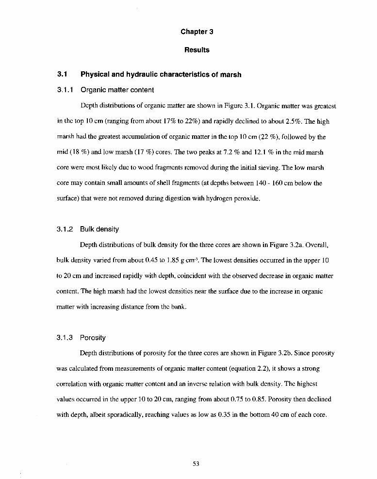
Chapter 3
Results
3.1 Physical and hydraulic characteristics of marsh
3.1 .I Organic matter content
Depth distributions of organic matter are shown in Figure 3.1. Organic matter was greatest
in the top 10 cm (ranging from about 17% to 22%) and rapidly declined to about 2.5%. The high
marsh had the greatest accumulation of organic matter in the top 10 cm (22 %), followed by the
mid (18 %) and low marsh (17 %) cores. The two peaks at 7.2 % and 12.1 % in the mid marsh
core were most likely due to wood fragments removed during the initial sieving. The low marsh
core may contain small amounts of shell fragments (at depths between 140 - 160 cm below the
surface) that were not removed during digestion with hydrogen peroxide.
3.1.2 Bulk density
Depth distributions of bulk density for the three cores are shown in Figure 3.2a. Overall,
bulk density varied from about 0.45 to 1.85 g ~ m - ~ . The lowest densities occurred in the upper 10
to 20 cm and increased rapidly with depth, coincident with the observed decrease in organic matter
content. The high marsh had the lowest densities near the surface due to the increase in organic
matter with increasing distance from the bank.
3.1.3 Porosity
Depth distributions of porosity for the three cores are shown in Figure 3.2b. Since porosity
was calculated from measurements of organic matter content (equation 2.2), it shows a strong
correlation with organic matter content and an inverse relation with bulk density. The highest
values occurred in the upper 10 to 20 cm, ranging from about 0.75 to 0.85. Porosity then declined
with depth, albeit sporadically, reaching values as low as 0.35 in the bottom 40 cm of each core.

Organic matter content (%)
100-
200
Figure 3.1: Organic matter content (% by mass) vs depth for low, mid and high marsh sites
-OH __-----
--------._._l-l- - - - - -. . . - - -----
, I
I-. - . Mid marsh *-.
-, - High marsh
0.0 5.0 10.0 15.0 21

* * - -
- . Mid marsh *.--
- High marsh
Bulk density (g/ml)
I . - -. Low marsh - - Mid marsh I I - High marsh1
Porosity
Figure 3.2: Bulk density (a) and porosity (b) vs depth for three cores for low, mid and high marsh sites.

The decline in porosity is due mainly to decreasing organic matter content, bioturbation, and
increasing sand content with depth.
3.1.4 Macroporosity
Estimates of macroporosity, based on changes in volumetric water content taken on July
28, 1993 are shown in Table 3.1. Values ranged from 0.03 to 0.17 indicating that, in the upper 30
cm, about 5-30% of the total pore space is composed of macropores. Macroporosity generally
decreased with depth below the surface and distance from the bank. The highest value (0.17)
occurred at the surface only 1 m from the bank.
3.1.5 Grain size distribution
Grain size distributions for clay, silt, and sand (taken from the low, mid and high marsh)
are shown in Figures 3.3a, 3.3b and 3.3c, respectively. These results confirm previous studies
which indicate a fining-upward sequence in marsh sediments. Clay content was usually greatest in
the top 20 cm (maximum of up to 23%) and then decreased rapidly with depth to below 5% in all
cores. Percent silt ranged from about 30 to 70% in the upper 100 cm and also declined with depth.
All three cores showed a slight increase in fines at about 120 to 130 cm below the surface. Sand
content showed an inverse trend, increasing with depth, reaching maximum values of around 80%
between 90 and 130 cm below the surface. The coarse fraction consisted of mainly fine sand (less
than 0.10 mm in diameter). The sediment can be classified as a silt loam in the upper 50 cm
grading to a (fine) sandy loam or loamy (fine) sand at greater depths, using the textural
classification system outlined in Hillel (1982, p. 28-29).
Horizontal trends within the cores were more difficult to determine. The low marsh core
(only 7 m from the bank) had the lowest sand content in the upper 100 cm but the greatest clay
content over the same interval. This seems to be somewhat atypical of tidal marshes which
generally show a decrease in grain size with decreasing distance from the bank, as larger particles
would tend to settle out first near the bank. Silt content in the upper 20 cm was highest in the mid

Table 3.1 : Changes in water content (8"; % by volume) at high and low tide and estimated macroporosity (%) from cores extracted on July 28, 1993.
Distance Depth to Depth below OV OV Macro- from river water table surface (cm) High Tide Low Tide porosity bank (m) (cm) ("4
Notes: numbers in brackets are standard errors.

- - Low Marsh I ......... Mid Marsh
-- High Marst
1 0 2 0 0 Clay (%)
\ \ - -
7 Low Marsh
......... Mid Marsh
I -- High Marsh
0 2 0 4 0 6 0 8 0 Silt (%)
- - Low Marsh /
......... Mid Marsh -- High Marsh
\'
Sand (%)
Figure 3.3: Result of grain-size analysis showing (a) percent clay (b) percent silt (c) percent sand vs depth at low, mid and high marsh locations. Note different scales on x-axes.

marsh core, possibly due to entrapment of suspended sediments by standing vegetation during tidal
inundation.
The mid marsh core also had a sharp increase in sand content (43%) between 20 and 30
cm below the surface, more than twice the value measured from the other two locations. Isotopic
dating of this core by Turner (1995) indicated that the Cs13' peak also occurred between 20 and 30
cm below the surface. Assuming that the date of maximum Cs137 concentration occurred in the year
1963, the peak of nuclear arms testing (Sharma et al., 1987), the relatively high sand content may
be the result of increased deposition during extreme high water which occurred in the summer of
1964 (Turner, 1995).
3.1.6 Hydraulic conductivity
The results discussed throughout this section are based on the method of Hvorslev (1951).
For a complete description and comparison of the results of the three methods (Luthin and
Kirkham, 1949; Hvorslev, 1951; Bouwer and Rice, 1976) see appendix 1.
3.1.6.1 Spatial variability
Hydraulic conductivity varied over 3 orders of magnitude in Musqueam Marsh and
generally decreased with depth (Figure 3.4). The highest conductivities occurred within the upper
50 cm. The geometric mean of hydraulic conductivity measured between 20 to 40 cm below the
surface (n = 8) was 1.14 x m s-I compared to 1.36 x m s-I between 40 to 60 cm below the
surface (n = 14). Conductivity decreased with depth throughout the upper sediment layers with a
geometric mean (n = 10) of 3.20 x lo-' m s-I between 80 and 120 cm below the surface.
Between 130 and 150 cm below the surface, hydraulic conductivity increased to an average of (n =
12) 5.13 x lo-' m s-I. This rise in hydraulic conductivity may be the result of increased sand content
(around 80%) at depths greater than 100 cm below the surface. Conductivity then increased
slightly between 160 to 200 cm (n = 6) below the surface (5.53 x m s-I), again due to increased
sand content at these depths.

..... ...- Slug test ......... Lowmarsh
Hydraulic conductivity (m/s)
- - Midmarsh
- - High marsh
Figure 3.4: Saturated hydraulic conductivity (mls) vs depth from 46 piezometers (solid squares) and grain-size analysis from three cores (dashed lines). The solid line represents a lowess (best fit) line to the measured conductivities.

The decrease in hydraulic conductivity in the upper sediment layers is possibly due to
decreasing biotic activity and root density. Although sediment in the upper 50 cm is mainly silt,
macropores created by burrowing organisms andor roots may transmit water through normally
low conductivity sediment. This effect is most apparent at a piezometer in the marsh interior 47 cm
below the surface and about 72 m from the river bank. Hydraulic conductivity at this piezometer
(3.32 x m s-I) was the highest of any of the 46 piezometers, and was more than an order of
magnitude greater than the geometric mean (1.38 x lo4 m s-') measured at a depth of about 50 cm.
This piezometer was located near a small stand of Typha latifolia, found in abundance in the mid
marsh, and may have been connected to the abandoned rhizome channels of this species.
Box plots of hydraulic conductivity vs. distance from the bank are shown in Figure 3.5.
Although considerable range occurs within each of the nine groups, usually up to half an order of
magnitude, the results suggest that at similar depths, hydraulic conductivity does not vary
significantly with distance from the bank.
3.1.6.2 Evaluation of relations with texture
Comparisons of hydraulic conductivity based on grain size distribution (Kgs; in 10 cm
intervals) from three cores and slug test data (K,) are shown in Figure 3.4. In the upper 80 cm,
estimates of Kgs from the three cores agreed reasonably with the result of slug tests performed in
piezometers. Below about 80 cm, estimates of Kgs were over an order of magnitude greater than
values of K,.
Agreement between the two methods near the surface was most likely due to the
macropores created from root channels and burrowing organisms. The differences between
conductivities below 80 cm were due primarily to other physical characteristics of the sediment
specific to this location. At lower depths compaction of the sediment and decreased organic matter
content resulted in hydraulic conductivities, based on in situ measurements (KJ, that ranged from
lo-' to 10" m s-I. However, modeled values (Kgs) yielded higher estimates around m s-I , typical
of "clean sand" (Freeze and Cherry, 1979, p. 29).

Coded distance from bank
Figure 3.5 ;: Box plots of hydraulic conductivity vs depth: (a) piezometers less than 80 cm below the surface, (b) between 80 and 120 cm below the surface and (c) greater than 120 cm below the surface. The codes along the X axis indicate distances for the bank. Code 1 is within 10 m from the bank, code 2 between 10 and 20 m from the bank, and code 3 greater than 20 m from the bank.

3.2 Hydrology of marsh
3.2.1 Evaporation
Rates of open-water evaporation (EJ, determined during tide-out periods are shown in
Table 3.2. Evaporation varied amongst days but daily totals were generally less than 1 mm during
tide-out periods on clear days. Tide-out conditions (low tide) typically lasted between 6 and 7
hours depending on timing and height of high and low water.
Hourly rates of El, increased through the morning and peaked in early afternoon consistent
with the expected diurnal variation of energy availability (e.g. Figure 3.6). The daily totals
generally followed the expected seasonal patterns of energy availability, with a decreasing trend
from August through September for clear-sky conditions (Table 3.2). The particularly low value of
El, for October 7 was probably caused by overcast sky conditions.
Evaporation measured under the cover of flattened vegetation (EJ was negligible during
tide-out periods on both clear and overcast days. The flattened vegetation effectively shaded the
surface and limited vapour transport away from the surface. During measurement, water levels in
the mariotte chamber actually increased slightly, indicating that water was added to the lysimeter
(i.e. negative rate of evaporation). This apparent increase was most likely due to organic debris
falling into the lysimeter (raising the water level) or from water dripping from the vegetation into
the ly simeter.
3.2.2 Flow net analysis
Figure 3.7 illustrates the evolution of the subsurface flow system at approximately one-
hour intervals during the tide-out period on September 3, 1993. On this day tidal range was 3.4 m
(Environment Canada, 1993b) and the sky was clear all day. The general pattern described here
was also observed on other days with similar tidal and climatic conditions (i.e. August 4th,
September 2 and 3, 1993). Some minor variations occurred amongst days depending on tidal range.
The tide dropped below the soil surface before 10:OO. Head levels in piezometers were
similar to tidal height indicating little or no movement of water in either horizontal or vertical

Table 3.2: Daily rates of open-water evaporation (Eo; mm), measured using mariotte lysimeters, on five days. Tide-out periods typically last for 6 - 7 hours.
Date (1 993) Open-water evaporation Conditions
August 4 0.78t clear all day
September 2 0.60 clear all day
September 3 0.72 clear all day
September 17 0.51 clear all day
October 7 0.08 overcast all day
Notes: t based on half-day measurements

Figure 3.6:Hourly evaporation measured from lysimeters on September 3, 1993. The numbers in the bars indicate the number of lysimeters in operation during that interval. Total evaporation for the day was 0.72 mm.

Piezorneter Distance From Bank (m) - - Equipotential (rn) - Flow line n K = 1.14~10-6_rn/s
Figure 3.7: Evolution of subsurface flow regime at (a) 9:45, (b) 10:45, (c) 11 :45 and (d) 13:00 on September 3, 1993.

" I I I I I I I I I I I I I I I I I I -2 0 2 4 6 8 10 12 14
Distance From Bank (m)
Piezometer - - Equipotential (m) - Flow line
Figure 3.7: Evolution of subsurface flow regime at times (e) 14:15 (f) 15:30 and (g) 16:15 on September 3, 1993.

directions. For example, at 09:45 tidal height was 2.79 m (relative to a common datum) whereas
head levels in the piezometers ranged from 2.76 to 2.83 m, indicating little, if any, detectable flux
of interstitial water. At 10:45 the water table had dropped about 5 cm. In the upper 1 m of
sediment, gradients were low but indicated a flux of water towards the bank. Gradients continued
to develop as the tide receded. Figure 3.7d shows the steepening of the hydraulic gradient near the
bank, indicated by the decreasing distance between equipotentials. Refraction of equipotentials
across the sediment boundaries indicated that above about 80 cm, flow is both horizontal (toward
the bank) and vertical (downward), while below 80 cm, interstitial water movement was
dominantly downward.
Around 1 :00, the tidal height dropped to the level of the sandy river sediments below the
fine sediments of the marsh. Water levels in piezometers on the sand flats indicated that interstitial
water was moving upward and seepage occurred along the sand flats (Figure 3.7d). The steepest
gradients developed during lowest low tide (LLT). Consequently, interstitial water movement was
greatest at this time. Following LLT, head levels in the piezometers began to equilibrate with tidal
height as the tide began to rise, decreasing the gradient within the sediment, but lagged behind the
rapidly rising tide. The deepest piezometers responded more rapidly than the shallow piezometers.
More than 10 m from the bank, however, interstitial water continued to flow downward. Note that
the flow regime at 15:30 is somewhat different from that at 11:45, even though the tidal height was
similar.
At 16:15 the tide had risen almost to the marsh surface (Figure 3.7g). The configuration of
the water table indicated that tidal water infiltrated through the bank, replenishing the water which
had drained out. Head measurements in piezometers indicated that interstitial water continued to
flow from the marsh interior toward the bank producing a zone of convergence about 2 m from the
bank.
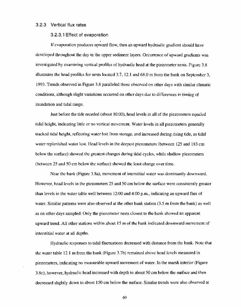
3.2.3 Vertical flux rates
3.2.3.1 Effect of evaporation
If evaporation produces upward flow, then an upward hydraulic gradient should have
developed throughout the day in the upper sediment layers. Occurrence of upward gradients was
investigated by examining vertical profiles of hydraulic head at the piezometer nests. Figure 3.8
illustrates the head profiles for nests located 3.7, 12.1 and 68.0 m from the bank on September 3,
1993. Trends observed in Figure 3.8 paralleled those observed on other days with similar climatic
conditions, although slight variations occurred on other days due to differences in timing of
inundation and tidal range.
Just before the tide receded (about 10:00), head levels in all of the piezometers equaled
tidal height, indicating little or no vertical movement. Water levels in all piezometers generally
tracked tidal height, reflecting water lost from storage, and increased during rising tide, as tidal
water replenished water lost. Head levels in the deepest piezometers (between 125 and 183 cm
below the surface) showed the greatest changes during tidal cycles, while shallow piezometers
(between 25 and 50 cm below the surface) showed the least change over time.
Near the bank (Figure 3.8a), movement of interstitial water was dominantly downward.
However, head levels in the piezometers 25 and 50 cm below the surface were consistently greater
than levels in the water table well between 12:OO and 4:00 p.m., indicating an upward flux of
water. Similar patterns were also observed at the other bank station (3.5 m from the bank) as well
as on other days sampled. Only the piezometer nests closest to the bank showed an apparent
upward trend. All other stations within about 15 m of the bank indicated downward movement of
interstitial water at all depths.
Hydraulic responses to tidal fluctuations decreased with distance from the bank. Note that
the water table 12.1 m from the bank (Figure 3.7b) remained above head levels measured in
piezometers, indicating no measurable upward movement of water. In the marsh interior (Figure
3.8c), however, hydraulic head increased with depth to about 50 cm below the surface and then
decreased slightly down to about 150 cm below the surface. Similar trends were also observed at
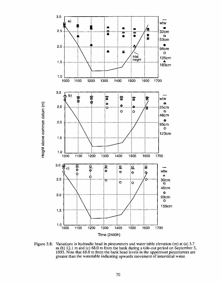
Time (2400h)
Figure 3:s: Variations in hydraulic head in piezometers and water table elevation (m) at (a) 3.7 m (b) 12.1 m and (c) 68.0 m from the bank during a tide-out period on September 3, 1993. Note that 68.0 m from the bank head levels in the uppermost piezometers are greater than the watertable indicating upwards movement of interstitial water.
70

three other stations in the marsh interior on this day as well as on September 2 and 3, 1993. Fluxes
at this station were upward from 50 cm below the surface and downward from 50 cm indicating a
zero flux plane somewhere around 50 cm.
The apparent upward flux of water near the bank, inferred from head measurements in
piezometers, may be a result of the slow response time of piezometers compared to that of water
table wells. Using equation 2.7 and assuming an average hydraulic conductivity of 1 x m s-I for
the upper 50 cm, a piezometer at that depth has a lag time (To) of about 13 minutes. Assuming
similar dimensions and conductivity for the water table well but a screen length of 0.5 m instead of
0.1 m (because the water table well is perforated over its entire length), the water table well has a
Ti, of about 4 minutes. As a result, water table wells respond up to 3 times faster to changes in
ambient head compared to piezometers. Moreover, wells near the banks were usually longer than
0.5 m in length, resulting in even shorter response times. Assuming an intake length of 1 m, Ti,
would be just under 2.5 minutes.
Upward fluxes due to evapotranspiration on October 7 should have been much lower than
those observed on September 3. Tidal range on October 7, 1993 was just 0.8 m (Environment
Canada, 1993b). The sky was overcast throughout the tide-out period and open-water evaporation
was about 0.1 mrn (Table 3.2). Piezometer response to tidal fluctuations at distances of 3.7, 12.1
and 68.0 m from the bank on October 7, 1993 are shown in Figure 3.9. Variations in hydraulic
head on October 7 are somewhat dampened due to the small tidal range. Hydraulic head increased
with distance from the bank and tracked tidal height at all depths. Fluxes were downward
throughout the tidal cycle, but head measurements near the bank also indicated an apparent vertical
flux of water upward. The upward flux observed near the bank on this day (and on Sept 3) is most
likely due to the lagged response of piezometers because the apparent flux occurred on days with
high and low evaporation rates. In the marsh interior, upward fluxes were observed at all
piezometers sites.

- wtw I
32cm 0
53cm
96cm 0
125cm A
1 83cm
- wtw
m 25cm
0
48cm @
95cm 0
123cm
- wtw
i3
30cm 0
46cm 0
99cm 0
159cm
900 1000 1100 1200 1300 1400 1500 1600
Time (2400h)
Figure 3:9: Variations in hydraulic head in piezometers and water table elevation (m) at (a) 3.7 m (b) 12.1 m and (c) 68.0 m from the bank during a tide-out period on October 7, 1993.

3.2.3.2Vertical velocities
Interstitial water velocities for piezometer nests 3.7, 12.1 and 68.0 m (the same stations
examined in the previous section), on September 3, 1993, are shown in Figure 3.10. Similar
velocity profiles were observed on other days with similar conditions. The greatest downward flow
was between the deepest piezometers closest to the bank. In the marsh interior (68.0 m from the
bank) upward fluxes less than 1 mm hrl were observed. Velocities measured on October 7, 1993,
were lower than those on September 3, due to limited tidal range and shorter tide-out period.
Overcast conditions also curtailed upward fluxes on this day, but fluxes were still observed in the
marsh interior (Figure 3.1 1).
3.2.3.3 Density driven flow
Vertical salinity differences between two adjacent piezometers were never more than 5 ppt
and typically occurred in the upper 100 cm of sediment during the winter months, when more dense
tidal water would overly less dense interstitial waters. Based on equation 2.13, the downward
velocity of interstitial water for the maximum observed difference in salinity (i .e. 5 ppt) was about
0.04 mm hr l or about 0.28 mm d-I (assuming a tide-out period of 7 hours). However, differences in
salinity between two piezometers were usually around 2 or 3 ppt resulting in pore water velocities
of 0.1 1 and 0.15 mm d-I, respectively.
3.2.4 Horizontal velocities
As the flow nets indicate, horizontal gradients decreased with distance from the bank and
were generally less than vertical gradients throughout the marsh. Horizontal velocities on
September 3, 1993, based on water table elevations, ranged from 0.22 to 1.10 mrn hr ' , within 5 m
of the bank and 0.02 to 0.41 mm hrl at distances greater than 5 m from the bank. Similar velocities
were also calculated from piezometers 50 cm below the surface. At approximately 150 cm below
the surface, horizontal fluxes were lower than velocities observed near the surface (0.17 - 0.70 rnrn
hrl within 5 m of the bank and 0.2 - 0.11 mm hrl at distances greater than 5 m from the bank).

WTW and 30cm WTW and 50cm 30 and 50cm 100 and l5Ocm
WTW and 30cm WTW and 50cm 30 and 50cm 100 and 150cm
WTW and 30cm 30 and 50cm
50 and 100cm 100 and 150cm
900 1000 7100 1200 1300 1400 1500 1600
Time (2400 hours)
Figure 3.10: Vertical interstitial water velocities (mrnlhr) during the tide-out period on September 17, 1993 for piezometer nests at (a) 68.0m for the bank, (b) 12.lm from the bank and (c) 3.7m from the bank. Positive fluxes denote upwards flow and negative downwards flow. Note different scales on y-axes.

3.0
2.0
1 .o - -. WTW and 30cm 0.0 - - WTW and 50cm
- - - - - - - 30 and 50cm -1 .o - - - . 100 and 150cm
-2.0
-3.0
-4.0 900 1000 1100 1200 1300 1400 1500 1600
3.0 L
I= \
E 2.0 E V
2 1.0 .- 0 0 - . WTW and 30cm - al 0.0 > ------. 30and50cm L - - - . 2 -1.0 100 and 150cm
s - (d -2.0 .- C .- C
C C - -0 -4.0
900 1000 1100 1200 1300 1400 1500 1600
Time (2400 hours)
WTW and 30cm 30 and 50cm
50 and 100cm 100 and 1 50cm
Figure 3.11: Vertical interstitial water velocities (mmlhr) during the tide-out period on October 7, 1993 for piezometer nests at (a) 68.0 m for the bank, (b) 12.1 m from the bank and (c) 3.7 m from the bank. Positive fluxes denote upwards flow and negative downwards flow.

The lower velocities at depth are due, in part, to the decreased horizontal gradients below 100 cm
below the surface (Figure 3.7) and to the lower hydraulic conductivity of the sediment. Horizontal
fluxes measured on October 7, 1993, were approximately 30% of those on September 3 due to
limited tidal range and, therefore, reduced driving force for flow. As with vertical flow, horizontal
velocities generally tracked tidal height, reaching minimum values during flooding and ebbing tide
and maximum values between 13:00 and 15:00, near the lowest tide of the day.
Seepage at the bank, based on horizontal flux velocities, ranged from 15-80 L m-I d-I. The
lower limit (15 L m-I d-I) was calculated using data from October 7, 1993 and the upper limit
(about 80 L m-1 d-I) using data from September 3, 1993. Seepage rates on September 3 were
greater due to a relatively larger tidal range and longer tide-out period.
3.2.5 Water cycling
If it is assumed that all water lost by drainage and evapotranspiration during low tide is
replaced by inundating water at high tide, then the amount of water replaced per tidal cycle can be
estimated by measuring the amount of water lost over one complete tidal cycle.
3.2.5.1 Water content
Spatial distributions of water losses during a tidal cycle, measured on July 28, 1993, are
shown in Table 3.1. The greatest observed water loss, 17% by volume, occurred 1 m from the
bank. Volumetric water loss was only 3% at 30 m from the bank over the same time interval.
Increased water table drawdown at low tide promoted drainage of interstitial water at the bank.
3.2.5.2 Residence times
Residence times increased with increasing distance from the bank (Table 3.3). In the upper
20 cm, average residence time of interstitial water in the low marsh (1 m from the bank) was about
1.7 days (or 3.2 tidal cycles). In the marsh interior, 30 m from the bank, residence time was almost
double that estimated at the bank (3.0 days or 5.8 tidal cycles). Drainage and cycling of water is

Table 3.3: Residence time of interstitial water (in tidal cycles and days), based on changes in water content at low and high tide, from July 28, 1993. Residence times were calculated after the method of Agosta (1985).
Distance from river Depth below Residence Time Residence Time bank (m) surface (cm) (tidal cycles) (days)+
Notes: t determined using 1.93 tidal cycles per day.

greatest near the bank. In the marsh interior, the water table may remain at or near the surface
resulting in little change in water content between high and low tide. Residence times also generally
increased with depth below the surface. Variability with depth is mainly due to changes in the
water table elevation at high and low tide and the increased macroporosity of the upper sediment
layers.
3.2.5.3 Water table drawdown and water loss
If water loss occurs primarily through drainage of macropores, as suggested by Harvey
and Nuttle (1995), then there should be a relation between water table drawdown and water loss at
a given location which would reflect the vertical profile of macroporosity. If the profiles of
macroporosity are similar from site to site, then the relation between water loss and water table
drawdown would provide a convenient alternative to direct measurement of water loss by
extracting cores, which is labour intensive. Water table drawdown is relatively simple to measure,
and does not involve destructive sampling.
Water table drawdown vs. depth of water loss is shown in Figure 3.12. Although based on
only five points, a positive relation exists between drawdown and the amount of water lost (rnrn)
per tidal cycle. The regression was run to pass through the origin as a water table drawdown of 0
cm would correspond to a water loss of 0 mm. Lack of time prohibited the collection of more
samples.
3.2.6 Water balance calculations
Results of the water balance calculations, for cells near the bank and in the marsh interior,
for five days are shown in Tables 3.4a and 3.4b, respectively. Horizontal fluxes throughout the
marsh were low on all days (less than 0.3 mm) and accounted for less than 5% of water lost from
the sediment. In contrast, downward vertical fluxes (qv) accounted for most of the water lost (>
85%), followed by evaporative losses (qc). Evaporative water loss was negligible near the bank
where downed vegetation prevent evaporation from the sediment.

Figure 3.12: Water table drawdown (cm) vs water loss (mm) in the unsaturated zone based on changes in water content (% by mass) taken at high and low tide.

Table 3.4a: Water losses (mm) estimated at a site 10 m from the bank on five days.
Date (1 993)
Length Lowest q, q, q,,,,,, q,,, Water loss Water loss of Tide- Tide (mm) (mm) (mm) (mm) flux water out (hrs) (m) estimate content
(mm) (mmY
Aug 6 7 1.8 7.4 0.0 0.1 7.3 7.6
Sept 2 7 1.7 7.8 0.0 0.3 0.1 8.0 7.2
Sept 3 7 2.0 6.1 0.0 0.2 0.1 6.2 7.2
Sept 17 7 1.8 6.4 0.0 0.2 0.1 6.5 6.8
Oct 7 6 3.3 2.5 0.0 0.1 0.1 2.5 4.6
Notes: t based on water table drawdown (figure 3.1 1) q, vertical (downwards) flux from cell q, evaporative flux from cell q,(,, horizontal flux into cell q,(,,,, horizontal flux out of cell
Table 3.4b: Water losses (mm) estimated at a site 60 m from the bank on five days.
Date Length Lowest q, q, q,,,,,, q,,, Water loss Water loss (1993) of Tide- Tide (mm) (mm) (mm) (mm) flux water
out (hrs) (m) estimate content (mm) b'mt
Aug 6 7 1.8 7.2 0.8 0.1 0.0 8.1 -
Sept 2 7 1.7 5.8 0.6 0.1 0.1 6.4 5.1
Sept 3 7 2.0 6.4 0.7 0.1 0.1 7.1 5.5
Sept 17 7 1.8 6.8 0.5 0.2 0.1 7.4 4.7
Oct 7 6 3.3 4.1 0.1 0.1 0.2 4.1 3.7
Notes: t based on water table drawdown (figure 3.1 1) q, vertical (downwards) flux from cell q, evaporative flux from cell q,,, horizontal flux into cell q,(,,,, horizontal flux out of cell

Water loss, based on water table drawdown (Figure 3.12), is also shown in Table 3.4.
Despite problems with lagged piezometer response, lateral flow, and lack of direct measurements
of water content, the two methods were within an order of magnitude. Estimates of water loss using
both methods on October 7, 1993, were the lowest of the five days sampled, due to overcast
conditions, small tidal range and shorter tide-out period. Lack of water table wells in the marsh
interior on August 6 prevented calculation of water loss based on water content.
3.3 Water Chemistry
3.3.1 Salinity
River and tidal salinity increased throughout the study period due mainly to the decreased
discharge of the Fraser River during winter months (Figure 3.13). The lowest salinities (less than 5
ppt) were recorded in May and early June of 1993 and the highest salinities (greater than 17 ppt)
were observed in January 1994. River water samples were usually collected at low tide except on
July 13 (Julian Day 194) and July 26 (Julian Day 207), which were sampled just after high tide. As
a result, the salinity values for those two days tended to show close similarity with inundating tidal
water. Figure 3.14 shows the relation between daily discharge and inundating tidal water salinity.
Interstitial salinity measured from all piezometers and pore water sampling wells ranged
from 4 to 21 ppt. The lowest salinities (less than 5 ppt) occurred in the interior stations (in the
shallowest piezometers or at the surface) during summer, with the highest values, greater than 20
ppt, at the bank stations (at the surface) in the winter months. Thus the marsh can be classified as
dominantly mesohaline (5.1 to 18.0 ppt) but may become mildly polyhaline (18.1 to 30.0 ppt)
during the winter months, based on the Venice classification system (Bulger et al., 1994).
Temporal changes in salinity with depth were greatest in the low marsh nearest the bank in
the upper sediment layers due to strong downward gradients and desaturation of sediment at low
tide (Figure 3.15). Salinity varied by up to 13 ppt (7 to 20 ppt) at a depth of about 30 cm below
the surface compared to just 4 ppt (1 1 to 15 ppt) at about 180 cm below the surface. Salinity
increased with depth from May to October 1993, and then decreased with depth for the rest of the

roc Jan 1 (1993) May i (1993) sept '1 (1 993) Jan 1 (1994)
Julian Day
3 Figure 3.13: Daily Discharge (m Is) of Fraser River near Hope (190 krn east of Vancouver) in 1993, inundating tidal water salinity (ppt) and surface water salinity in the North Arm adjacent to the study site vs time.
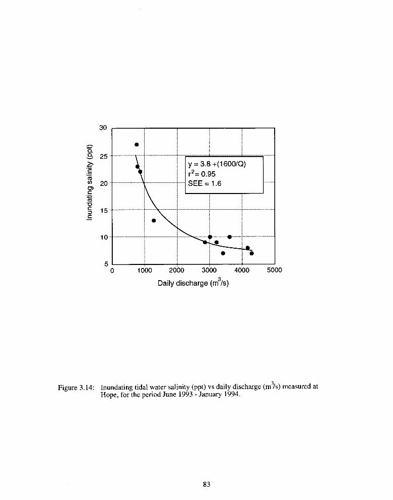
0 1 000 2000 30'00 4600 5000
Daily discharge (m3/s)
Figure 3.14: Inundating tidal water salinity (ppt) vs daily discharge (m3/s) measured at Hope, for the period June 1993 - January 1994.

Pore Date water ( 1 993) salinity - Jun 09
- - Jul06
- - Aug 13
- - - - Sep 30 ....... Nov 23 . - Dec 20
Xdal water salinity no dam
0
0
0
A
Pore Date water (1993) salinity nodam Jun 09
- - JuI 06 - - Aug 13
- - - - Sep 30 ........ Nov 23 - - Dec 20
Tidal water salinity no dam
0
w 0
0
A
Tidal water salinity no dam
0
Salinity (ppt)
Figure 3.15: Salinity profiles at (a) 3.7 m (b) 12.1 m and (c) 68.0 m from the bank.

year until spring of the following year reflecting the change in inundating tidal water. A similar
profile was observed at a piezometer nest 12.1 m from the bank (Figure 3.15b). As with stations
closer to the bank, salinity typically increased with depth between spring and early fall, and then
decreased throughout the rest of the year.
3.3.2 pH
The pH of the river water ranged from about 6.8 to 8.1 throughout the sampling period.
River water was slightly acidic in May 1993 and generally increased throughout the sampling
period, reaching a maximum in October 1993. The pH range of inundating tidal water was much
more limited (6.9 - 7.6) but generally increased throughout the year. The changes in river pH
reflect the influence of the spring freshet and (more basic) sea water on river acidity.
Overall, interstitial pH ranged between 6.05 to 7.45 and followed a similar pattern to that
for river pH. The highest values occurred at the bank station in the winter months with the most
acidic conditions (pH c 7) occurring in the interior sites during the spring and summer months.
Interstitial pH increased throughout the entire sampling period at all depths (Figure 3.16). In the
marsh interior, interstitial pH was greatest in the upper 50 cm of sediment possibly due to organic
acids produced from decaying organic matter. Near the bank a more complex pattern was
observed. Interstitial pH increased with depth throughout the sampling period (possibly a result of
increased organic matter content with depth), although the change in pH with depth is more gradual
compared to the interior station. For example, on August 16, pH ranged from 6.2 - 6.8 at the
interior station, compared to 6.3 - 6.5 near the bank.
As previously seen in profiles of salinity, the bank station may have more effective mixing
of pore water and tidal water producing profiles that are less variable with depth. The bank station
also shows the highest pH values in October 1993, coincident with the peak observed in the river
water, indicating a relatively rapid response. The interior station has the highest pH values in
January, in the upper 50 cm, indicating a response lag time of about 3 months.

June 17
0 Aug l6
Aug 27
A Oct 12
A Jan 5
200 ! t
6.0 6.2 6.4 6.6 6.8 7.0 7.2 7.4
pH
Figure 3.16: pH vs depth at (a) mid marsh, 60 m from bank, and (b) low marsh, 5 m from bank.

3.3.3 Redox potential
Reliable measurements of redox potential were difficult to obtain. Due to the nature of the
sampling procedure, pore water samples remained in the wells for up to 15 minutes after purging
was complete, possibly allowing for oxidation of the interstitial water being sampled (Freeze and
Cherry, 1979, p.141). This was done to obtain as much sample as possible because the finer
sediment made it difficult to fill the larger piezometers quickly. Moreover, the Hanna probe did not
stabilize to a constant value and tended to jump approximately & 5 mV. Redox values presented
here are the average of the two sampling nests at each location.
Overall, redox potential of the pore water varied from about +23 to -44 mV, indicating a
reduced soil, according to the classification system of Patrick and Mahaptra (1968). Depth profiles
from both stations show a slight decrease in depth with the greatest values occurring at 30 cm
below the surface (Figure 3.17). Increased aeration of the surface sediment during tide-out periods,
due to evapotranspiration and/or interstitial water movement, promotes oxidation of the upper
sediment layers while deeper layers remain reduced. However, redox potential at the bank station
was somewhat lower than that observed at the interior station even though drainage of sediment
was greatest at the bank at low tide. Lower potentials near the bank may be the result of reduced
interstitial water moving toward the bank during low tide.
Redox potentials were slightly positive during the summer months but became increasingly
negative in the fall and winter months. Lower redox potentials may be due to the higher tides in the
winter months which would cover the marsh surface for longer periods of time. Also, greater
evaporation rates and lower precipitation would tend to increase aeration of the sediment during the
summer months.
3.3.4 Heavy metals
Overall, pore water concentrations of heavy metals measured on August 12, 1993, and
January 5, 1994, were generally less than 200 ppb at most depths (Tables 3.5 to 3.8). Lead was
found at the highest concentrations of all four elements sampled and ranged from 76 to 277 ppb.

May 20
June 17
Aug 16
Aug 27
A Oct 12
A Jan 5
Redox potential (mV)
June 17
Aug 16
Aug 27
Oct 12
Jan 5
1 . I . I .
0 -40 -30 -20 -lb 0 10 20 : 1 . 1 . 1 '
Redox potential (mV)
Figure 3.17: Redox potential (mV) at (a) mid marsh, 60 m from the bank and (b) low marsh, 5 m from the bank.

Table 3.5a: Concentration of Cadmium (ppb) in the pore water of Musqueam Marsh 5 m from the bank on August 12, 1993 and January 5, 1994. Error in concentrations is 1 3 ppb.
Distance from river Depth below [Cdlt P P ~ [Cdlt PPb bank (m) surface (cm) August 12,1993 January 5,1994
Notes: t Tr = Trace amount of Cd present, below detection limit of Flame AA (Cd - 30 ppb) - no sample collected.
Table 3.5b: Concentration of Cadmium (ppb) in the pore water of Musqueam marsh, about 70 m from the bank (marsh interior) on August 12, 1993 and January 5, 1994. Error in concentrations is + 3 ppb.
Distance from river Depth below [Cdlt PPb [Cdlt P P ~ bank (m) surface (cm) August 12,1993 January 5,1994
Notes: t Tr = Trace amount of Cd present, below detection limit of Flame AA (Cd - 30 ppb) - no sample collected.

Table 3.6a: Concentration of copper (ppb) in the pore water of Musqueam Marsh 5 m from the bank on August 12, 1993 and January 5, 1994. Error in concentrations is + 3 ppb.
Distance from river Depth below [Cult PPb [Cult PPb bank (m) surface (cm) August 12,1993 January 5,1994
Notes: t Tr = Trace amount of Cu present, below detection limit of Flame AA (Cu - 30 ppb) - no sample collected.
Table 3.6a: Concentration of copper (ppb) in the pore water of Musqueam Marsh, about 70 m from the bank (marsh interior) on August 12, 1993 and January 5, 1994. Error in concentration is f 3 ppb.
Distance from river Depth below [Cult P P ~ [Cult PPb bank (m) surface (cm) August 12,1993 January 5,1994
Notes: t Tr = Trace amount of Cu present, below detection limit of Flame AA (Cu - 30 ppb) - no sample collected.

Table 3.7a: Concentration of lead (ppb) in the pore water of Musqueam Marsh 5 m from the bank on August 12, 1993 and January 5, 1994. Error in concentrations is f 20 ppb.
Distance from river Depth below [Pblt PPb [Pblt PPb bank (m) surface (cm) August 12 ,1993 January 5 ,1994
Notes: t Tr = Trace amount of Pb present, below detection limit of Flame AA (Pb - 120 ppb) - no sample collected.
Table 3.7b: Concentration of lead (ppb) in the pore water of Musqueam Marsh, about 70 m from the bank (marsh interior) on August 12, 1993 and January 5, 1994. Error in concentrations is f 20
P P ~ .
Distance from river Depth below [Pblt PPb [Pblt P P ~ bank (m) surface (cm) August 12 ,1993 January 5 , 1 9 9 4
Notes: t Tr = Trace amount of Pb present, below detection limit of Flame AA (Pb - 120 ppb) - no sample collected.

Table 3.8a: Concentration of Zinc (ppb) in the pore water of Musqueam Marsh 5 m from the bank on August 12, 1993 and January 5, 1994. Error in concentrations is 2 ppb.
Distance from river Depth below [Znlt PPb [Znlt PPb bank (m) surface (cm) August 12, 1993 January 5,1994
Notes: t Tr = Trace amount of Zn present, below detection limit of Flame AA (Zn - 20 ppb) - no sample collected.
Table 3.8b: Concentration of Zinc (ppb) in the pore water of Musqueam Marsh, about 70 m from the bank (marsh interior) on August 12, 1993 and January 5, 1994. Error in concentrations is k 2
P P ~ .
Distance from river Depth below [Znlt PPb [Znlt PPb bank (m) surface (cm) August 12,1993 January 5,1994
Notes: t Tr = Trace amount of Zn present, below detection limit of Flame AA (Zn - 20 ppb) - no sample collected.

Copper (30 - 112 ppb) and zinc (37 - 95 ppb) showed the next highest concentrations followed by
cadmium (34 - 68 ppb). Concentrations of cadmium, lead and zinc on August 12, 1993, were
generally lower than those measured on January 5, 1994. Zinc, often associated with stormwater
runoff, remained relatively high in August, possibly as a result of the approximately 100
stormwater discharges into the North Arm (FREMP, 1990~). Lower concentrations in the summer
may be due to increased uptake by plants (e.g. Environment Canada, 1989) or dilution of pore
water due to increased discharge during the spring freshet. It is unknown why the temporal pattern
of copper differs from the other metals.
Spatial distributions of metals were difficult to determine. Although there is much
variability in the data, it appears that concentrations of metals increased slightly with depth near
the bank and in the marsh interior. For example, the highest concentrations of Pb and Cd occurred
at depths greater than 150 cm below the surface. This was the opposite to what was expected
based on interstitial water chemistry. Heavy metals in the upper sediment layers would tend to
remain in solution, and therefore mobile, due to lower pH and higher redox potentials (Domenico
and Schwartz, 1990, p.456). However, strong downward fluxes during tide-out periods may have
transported aqueous phase metals near the surface to deeper sediment layers. Horizontal
distributions could not be adequately examined due to the lack of data.
3.3.4.1 Advective and diffusive fluxes of metals through sediment
Downward fluxes of metals near the bank were almost an order of magnitude greater than
both horizontal and upward flux rates (Table 3.9). Fluxes near the bank reflect relatively high
metal concentrations as well as high interstitial water velocities during tide-out periods. Vertical
flux rates from the marsh interior were low. As upward flow in the marsh was limited to tide-out
periods with favorable evaporation rates, enhanced upward fluxes of metals may only occur for
short periods of time during the summer months, as is the case with this data. Hence vertical
estimates recorded here must be treated with caution. Horizontal fluxes in the marsh interior 70 m
from the bank (not shown in Table 3.9) were less than half the values obtained near the bank.

Table 3.9: Maximum daily flux estimates of metals through marsh sediment based on heavy metal concentrations, from January 5, 1994, and average interstitial water velocities, from September 3, 1993, assuming a tide-out period of seven hours.
Metal Upward Flux Downward Flux Horizontal Flux (marsh interior) (bank) (bank) pg ~ r n - ~ d-I pg cm2 d-I pg ~ r n - ~ d-I

Using the maximum concentration gradients observed at Musqueam Marsh, fluxes based on
diffusion only (using equation 2.19) were lo5 - lo7 times lower than advective fluxes. For example,
on an annual basis maximum possible advective fluxes of Pb were estimated to be 80300 pg cm2
yr-I while maximum possible diffusive fluxes were only 0.012 pg cm2 yrl.
3.3.4.2 Relations to solid phase
Summary statistics of distribution coefficients for Cd, Cu, Pb and Zn are shown in Table
3.10. Given the difficulty in determining spatial and temporal trends in aqueous phase
concentrations, it was difficult to determine trends in distribution coefficients. The highest K,
values for Cu, Pb and Zn were found between about 30 - 50 cm below the surface. Distribution
coefficients (for Cu, Pb and Zn) appeared to decrease somewhat with depth as solid phase
concentrations dropped rapidly below about 50 cm below the surface (Turner, 1995) and pore
water concentrations increased slightly. The large range in K, values for Cu and Zn indicate high
spatial variability and the uncertainty in estimating K, values using equation 2.17.

Table 3.10: Summary statistics for estimated Kd values (rnL g-l) of Cd, Cu, Pb, and Zn.
Metal Number Average Range Standard of samples (mL g-'1 (mL g-') Deviation
(mL g-')
Notes: t calculated using solid phase Cd concentration from upper 20 cm (Environment Canada, 1989).
Chapter 4
Discussion
4.1 Physical Characteristics of Marshes
4.1.1 Vertical variation of conductivity
Slug test data from Musqueam Marsh indicated a decrease in hydraulic conductivity with
depth. Hydraulic conductivity determined from grain-size analysis increased with depth. Despite
the differences between the two methods (up to an order of magnitude), hydraulic conductivity at
Musqueam Marsh is generally within the silty sand range, typical of most marshes (e.g. Gardner,
1975; Knott et al., 1987). There are several possible reasons for the disparity between the two
methods. Although the surficial sediment has a high percentage of fines (silt and clay), it may also
contain high amounts of organic matter, primarily due to the high plant productivity in these
environments (Yamanaka, 1975). Macropores created by abandoned root channels and decaying
organic matter may allow rapid movement of water through fine-grained sediment (Knott et al.,
1987). The dominant sedges in Musqueam Marsh have rooting depths between 60 and 100 cm
(Karagatzides, 1988). This range corresponds with the rapid decrease in K around 100 cm below
the surface at Musqueam Marsh.
In marshes along the eastern United States, organisms, such as crabs or worms, are also
capable of reworking sediment and creating extensive networks of macropores (e.g. Nestler, 1977;
Bricker-Urso et al., 1989). Although I was unable to determine the effects of organisms at
Musqueam Marsh, bioturbation of the upper sediment does occur. Hutchinson et al. (1989) noted
that Snow Geese and Trumpeter Swans grub in the bare marsh surface for roots and rhizomes and
play a significant role in changing the microtopography of Fraser River marshes. Trumpeter Swans
were frequently observed at Musqueam Marsh between October and December, 1993.
Once organic matter content and biotic activity decrease below some critical value,
hydraulic conductivity is controlled by sediment texture. As sand content increases, hydraulic
conductivity should increase accordingly. However, at Musqueam Marsh, and in other studies

noted above, slug test data indicated that K remained low even in deeper, coarser, sediment. This
may be due, in part, to smaller sized material, such as clay or humus, filling in the larger pore
spaces between sand grains (Knott et al., 1987). Compaction caused by sediment loading may also
pinch off flow paths in deeper sediment layers. Hydraulic conductivity measured from slug tests
reflects not only the vertical profile of grain size, but also the distribution of organic matter and
biotic processes.
4.1.2 Horizontal variation in conductivity
At Musqueam Marsh, organic matter content, bulk density and grain-size distribution were
similar at all three locations within the marsh. Coincidently, box plots of in situ hydraulic
conductivity indicated that there was little difference between values 0 to 60 m from the bank.
Harvey et al. (1987) also observed similar patterns at the creekbank, levee and marsh flat locations
in a Virginia salt marsh. As tidal conditions, local topography, and sediment characteristics vary
significantly between estuaries, it is difficult to create a general model of lateral distributions of
sediment grain size and hydraulic conductivity. For example, Osgood and Zieman (1993) observed
no significant difference in grain size between high and low marsh stations, while Yelverton and
Hackney (1986) and Hutchinson (1982) noted a decrease with increasing elevation of the marsh
platform.
Although not observed at Musqueam Marsh, hydraulic conductivity may show strong
horizontal variability. The bank, or low marsh, zone is thought to increase productivity of marsh
vegetation due to higher rates of interstitial water movement and repeated drainage at low tides
(King et al., 1982; Howes et al., 1986). Larger plants tend to have greater rooting depths and
larger roots. Agosta (1985) observed that subsurface flow near the creekbank was, in fact, faster
than could be predicted by sediment permeability and hydraulic gradients, which suggested to her
that water was flowing through old Spartina root channels.

4.1.3 Temporal variation in hydraulic conductivity
As most of the slug tests at Musqueam Marsh were conducted over a three month period,
seasonal variability in K could not be adequately determined. Saturated hydraulic conductivity may
be affected by changes in the density and viscosity of the pore water due to variable concentrations
of cations (mainly sodium) in interstitial water. Dane and Klute (1977) observed that soil swelling
due to increased salinity may decrease hydraulic conductivity. Seasonal variations in salinity may,
in turn, promote fluctuations of K in sediments. Increases in pH have also been shown to decrease
hydraulic conductivity in some soils (Suarez et al., 1984). The effect of temperature on hydraulic
conductivity in intertidal sediments may be minimal relative to the effect of salinity (Section 2.6.4).
Seasonal variations may also be caused by vegetation. Knott et al. (1987) stated that hydraulic
conductivity of salt marsh soils may increase in the dormant season, and subsequently decrease
during the growing season, as roots grow and pinch off flow paths.
4.2 Hydrology
4.2.1 Regional groundwater flow
Subsurface flow at Musqueam Marsh was downward (down to about 2.3 m below the
surface) throughout the marsh during tide-out periods except for small vertical fluxes near the
surface, possibly due to evaporation and/or transpiration. Although topographically higher regions
around Musqueam Marsh could promote groundwater flowing upward through the sediments, a
freshwater creek approximately 700 m from Musqueam Marsh probably intercepts regional
groundwater which might otherwise enter the marsh sediments from the adjacent upland. Thus
regional groundwater discharges into the North Arm of the Fraser River as surface water several
hundred meters upriver of Musqueam Marsh (Figure 4.1). The microcliff at Musqueam Marsh
promoted strong downward fluxes of water during tide-out periods, possibly negating upward
fluxes from a regional aquifer. Upward flow did occur in the sandy intertidal sediments at tide-out
periods during low tide.

Figure 4.1 : Musqueam Marsh and surrounding environment (NTS 92Gl3g).

Some previous studies have indicated an upward flux of water through marsh sediments.
Harvey and Odum (1990) and Harvey and Nuttle (1995) observed significant upward flow in
marshes along the coast of Virginia. These marshes had gradual changes in slope and low
horizontal gradients, unlike Musqueam Marsh, allowing upward flow to dominate the subsurface
regime. Most other detailed studies of subsurface hydrology sampled only the upper 1 m of
sediment (using only water table wells or shallow depth piezometers) and did not consider larger
scale flow patterns (e.g. Agosta, 1985; Gardner, 1975; Harvey et al., 1987).
Discharge from a regional aquifer through estuarine sediments can not only alter
subsurface flow patterns, but can also control pore water chemistry. Further evidence of limited
regional flow into Musqueam Marsh can be seen in the chemical data. An upward flux of fresh
regional groundwater would produce salinity profiles that decreased with depth throughout the
season, with only limited variability at or near the marsh surface (Harvey and Odum, 1990). At
Musqueam Marsh, salinity increased with depth during the summer months and remained relatively
constant throughout the year between 1.5 to 2.3 meters below the surface.
4.2.2 Density-driven flow
Saline water overlying "fresh" interstitial water has an inherently unstable density gradient,
and will move downward, a process that Bokuniewicz (1992) called salt fingering. In Musqueam
Marsh, salt fingering is a minor component of the subsurface hydroregime. This study has shown
that downward fluxes of interstitial water were two orders of magnitude greater than downward
flow induced by salinity gradients. However, rates of density driven flow were similar to upward
fluxes due to evapotranspiration.
In many previous studies, density-driven flow was not considered (e.g. Harvey et al.,
1987; Harvey and Odum, 1990) even though strong salinity or electrical conductivity gradients
were observed at some locations (e.g. Harvey and Odum, 1990). In regularly inundated marshes
steep vertical salinity gradients may not develop due to pore water drainage and efficient mixing of
tidal and interstitial waters, especially near the bank. At Musqueam Marsh, density-driven flow
would be further limited to the winter months when inundating tidal water salinities are high. Due
to the conservative salinity range of interstitial water (6-24 ppt), and frequent tidal inundation,
density-driven flow appears to be low compared to hydraulic-gradient-induced flow in Musqueam
Marsh.
Density-induced flow may be an important process in irregularly inundated marshes where
the concentration of salt near the soil surface is high. Casey and Lassaga (1987) observed salinity
gradients of about 50 ppt cm-' throughout the summer months in the upper 20 cm of an irregularly
inundated marsh in Chincoteague Bay, Virginia. Using equation 2.14, density driven flow
velocities in Chincoteague Bay may be on the order of 5 - 10 rnm d-' and would continue even
during tidal inundation. Steep salinity gradients coupled with low hydraulic gradients may produce
dominantly downward fluxes of interstitial water for at least part of the year. Coarse grained (or
subtidal) sediment would also increase interstitial velocities caused by density gradients. For
example, Bokuniewicz (1992) estimated velocities of 5 cm hrl in sandy sediment (K = 2.2 x m
s-I) near Great South Bay, New York.
4.2.3 Subsurface flow in marsh sediments
Flow net analysis indicates that subsurface flow at Musqueam Marsh was controlled by
tidal height. As the tide ebbed, strong hydraulic gradients developed due to the increased slope in
the watertable, producing a net flow of interstitial water downward and toward the bank.
Refraction of flow lines across a sediment boundary, about 100 cm below the surface, suggested
that pore water flow may be somewhat horizontal in the upper 100 cm but dominantly downward
below about 100 cm. In the marsh interior, the water table remained relatively constant during tide-
out periods and horizontal gradients were lower than those near the bank. Upward fluxes of water
in the upper 50 cm were likely driven by evapotranspiration at the surface.
Subsurface flow at Musqueam Marsh is somewhat different from the general patterns
described in the literature. Other studies have found either horizontal flow throughout the marsh
sediment (e.g. Jordan and Correll, 1985) or an upward flux of water from a regional aquifer (e.g.

Harvey and Odum, 1990). As previously noted, a freshwater creek may capture groundwater that
would otherwise flow through the sediment of Musqeam Marsh. The influence of the microcliff,
which generated steep gradients at the bank, combined with well developed stratification of the
substrate, produced horizontal flow in the upper sediment layers and mainly downward flow at
depth. Some of the previous studies that predicted only horizontal flow may have shown flow
patterns similar to Musqueam Marsh if the effects of deeper strata were considered.
4.2.4 Seepage rates
Interstitial water velocity and seepage at the creekbank was greatest around low tide and
declined rapidly at Musqueam Marsh as the tide rose. Gardner (1975) and Yelverton and Hackney
(1986) noted that the maximum discharge occurred approximately twice per day at low tide due to
a semi-diurnal tidal cycle. Table 4.1 shows estimates of seepage flux rates (L m-I d-I) at several
different marshes, including this study. Estimates from Musqueam Marsh may be low as discharge
of interstitial water through the sandy river sediment was not considered in the calculation of
seepage flux.
Most of the flux rates in Table 4.1 vary by less than an order of magnitude, although some
differences are apparent. Variability in drainage fluxes may be due, in part, to marsh
characteristics (such as grain-size distribution and bank morphology) and/or different methods
employed to calculate fluxes. For example, the relatively low fluxes estimated by Harvey and
Odum (1990) in two Virginia marshes are possibly due to the low horizontal gradients observed at
both locations. Nuttle and Hemond (1988) stated that fluxes calculated using hydraulic gradients
and estimates of hydraulic conductivity are prone to large errors due to uncertainties in the
estimation of hydraulic conductivity. The relatively large range of drainage fluxes measured in this
study and by Agosta (1985) suggests that this may be true. However, Table 3.4 indicates that rates
of water loss (based on hydraulic head and hydraulic conductivity) were similar to estimates of
water loss based on water content at Musqueam Marsh. Therefore, in this case, estimates of

Table 4.1 : Pore water drainage mesured at various marshes. Modified from Nuttle and Hemond (1988).
Location Drainage Flux (L m-I d-l) Reference
Bread and Butter Cr, SC
Goat Island, SC
Carter Creek, VA
Eagle Bottom, VA
Chesapeake Bay, NC
Belle Island Marsh, Mass
Pender County, NC
Musqueam Marsh, BC
Agosta (1 985)
Gardner (1 976)
Harvey et a/. (1 987) Harvey and Odum (1 990)
Harvey and Odum (1 990)
Jordan and Correll (1 985)
Nuttle and Hemond (1 988)
Yelverton and Hackney (1 986)
this study

hydraulic head and hydraulic conductivity at Musqueam Marsh should be reasonable. The large
range in seepage rates at Musqueam Marsh is due mainly to variations in length of tide-out period.
4.3 Interstitial Water Chemistry
4.3.1 Salinity
Salinity at Musqueam Marsh showed strong seasonal variation, controlled ultimately by
the discharge of the Fraser River. Interstitial salinity was higher during the winter months and
lower during the summer months due to the dilution of inundating tidal water from increased
discharge of the Fraser River. Similar seasonal patterns have also been observed in other marshes
throughout the Fraser River Estuary (e.g. Chapman and Brinkhurst, 1981; Environment Canada,
1989). Salinity profiles increased with depth in the winter and decreased with depth in the summer.
Desaturation of sediment, due to drainage andor ET during tide out periods, produced lower
residence times compared to deeper sediment layers. Interstitial salinity closest to the bank
paralleled that of inundating tidal water, while in the marsh interior, salinity showed less variation
throughout the year due to reduced rates of subsurface flow.
Salinity profiles at Musqueam Marsh were different than those reported in similar studies.
In intertidal marshes in the southern United States, where most studies have taken place, interstitial
salinity increased in the summer due to high rates of evaporation (e.g. Hackney and de a1 Cruz,
1978; Zedler, 1983). Salinity typically decreases with depth (Casey and Lasaga, 1987) and
increases with increasing distance from microcliffs or tidal creeks (Nestler, 1977). Upwelling of
fresh groundwater from a regional aquifer may also produce salinity profiles that increase with
depth throughout the year (Lindberg and Harris, 1973; Harvey and Odum, 1990).
Spatial distribution of salt in Musqueam Marsh was also controlled by subsurface fluxes.
In sediments throughout the Fraser River Estuary, Chapman (1981b) noted that interstitial
salinities of subtidal sediments, containing a high proportion of silt, were relatively constant over a
tidal cycle despite large fluctuations in the salinity of overlying water. Although diurnal variations
in salinity were not measured at Musqueam Marsh, results suggest that interstitial salinity may

change rapidly in the upper sediment layers over one complete tidal cycle. Desaturation of sediment
during tide-out periods coupled with high macroporosity would allow tidal water to penetrate into
the upper 10-30 cm of sediment.
Large fluctuations in salinity were observed to depths of about 80 cm (Figure 3.15). Based
on advection alone, using data from September 3 and October 7 (extreme tidal ranges), inundating
water would reach a depth of 100 cm in about 37 and 58 days, respectively; surface water would
reach a depth of 200 cm in approximately 2 to 3 months. These times would be reduced further if
tidal water penetrated the upper 30 cm or so of sediment, which probably occurs when the marsh is
flooded. Diffusive fluxes of salt, usually several orders of magnitude less than advective fluxes
(Price and Woo, 1988a), would probably not produce the rapid changes in salinity observed at
Musqueam Marsh.
Penetration of tidal water at Musqueam Marsh may be even greater in winter months due
to density-induced flow from overlying saline water. Lindberg and Harris (1973) hypothesized that
convective interchange of saline tidal water and interstitial water was the dominant process
controlling pore water salinities in the upper 2.5 cm of a salt marsh in Florida. In laboratoly
experiments and in situ testing, Chapman (1981b) noted that overlying saline water exchanged
more rapidly with silt sediments containing relatively fresh water than the reverse. At Musqueam
Marsh, lag times based on salt penetration, noted above, may be slightly lower in the winter due to
density-induced flow.
4.3.2 pH
Interstitial pH at Musqueam Marsh showed strong temporal and spatial variability
controlled mainly by inundating tidal water, which is composed of river and sea water. The pH of
sea water is around 8.0 to 8.4 (Gardner, 1973). Rivers tend to be slightly more acidic and have a
much broader range of pH, with typical values between 6.9 and 8.0 (Stednick, 1991) depending on
such factors as precipitation and sediment origin. During the winter months, reduced flow of the

Fraser River caused an increase in interstitial pH. Similar results have been obtained from other
marshes in the Fraser River Estuary (e.g. Environment Canada, 1989).
At Musqueam Marsh, interstitial pH was higher near the surface possibly due to hurnic
acids (Ponnamperuma, 1968) derived from decaying organic matter. Oxidation of hydrogen sulfide
during tide-out periods also causes a lowering of pH (Gardner, 1975), as indicated by the following
reaction:
H,S + 20, -+ 2H+ + SO;, (4.1).
Casey and Lasaga (1987) noted a slight decrease in pH in the interstitial water during the summer
months. The pH typically ranged from 5.5 to 6.5 but decreased to between 4.0 and 6.0 in the
summer. Howes et al. (1986) also noted lower values of pH (3.5 - 4.0) of interstitial water during
extensive periods without flooding. With no input of (more basic) tidal water, the pH of interstitial
water may remain slightly acidic and further oxidation of sulfate may continue to lower the pH.
Due to alternating periods of oxidation and frequent tidal inundation, the pH of regularly inundated
tidal marsh sediments typically ranges between 5 and 7 (e.g. Yamanaka, 1975; Hackney and de la
Cruz, 1978). Musqueam Marsh also fits within the average range (6.1 - 7.5).
Data on the spatial distributions of pH within regularly inundated tidal marsh sediments
are limited. Yamanaka (1975) observed a decrease in pH towards the marsh interior (from about
7.0 to 6.0) in several marshes in the Fraser River Estuary. Snow (1982) also observed more acidic
pH in the marsh interior (sedge marsh) as compared to nearby mudflats. Interstitial pH was usually
greater than 7.0 on the mudflats and decreased to more acidic conditions in the sedge marsh (6.1-
6.8). A detailed study of interstitial water chemistry near Goat Island Virginia by Gardner (1973)
revealed similar profiles to those observed at Musqueam Marsh. Interstitial pH progressively
decreased towards the marsh interior with higher values of pH observed near the margins of tidal
creeks. Along the banks of tidal creeks, downward movement of interstitial water and desaturation
of sediments during low tide, allows the mixing of interstitial water and sea water resulting in more
basic interstitial water. In the marsh interior, limited tidal input results in interstitial water with a
relatively lower range of pH.

4.3.3 Redox potential
Redox potential at Musqueam Marsh varied from +23 to -44 mV typical of a reduced soil.
Profiles indicated a decrease in redox potential with depth throughout the season. Regularly
inundated marshes undergo reduction during inundation and oxidation when the tide recedes and
the sediment is aerated. Due to frequent inundation, high silt and clay content and prolonged
saturation, marshes are typically reducing environments and profiles of Eh in other marshes
generally decrease with depth (e.g. Long and Mason, 1983, p. 37; DeLaune et al., 1983; de a1
Cruz et al., 1989). In controlled experiments, Linthurst and Seneca (1980) noted that redox
potentials increased with increasing elevation (from -30 cm below the marsh surface to +10 cm
above the surface).
Subsurface fluxes of interstitial water may also regulate redox potentials in marsh
sediments. At Musqueam Marsh redox potential was slightly lower near the bank, compared to the
marsh interior, even though desaturation was greatest during low tide. In other studies, higher
potentials have been observed near the banks of tidal creeks (Howes et al., 198 1; de a1 Cruz et al.,
1989). Gardner (1973) noted that redox potential decreased with distance from a creek bank in a
South Carolina marsh. Along the margins of microcliffs or tidal creeks, strong downward flow
during tide-out periods would transport more oxidized water to deeper layers compared to interior
stations. Hence, sediment near the bank would have higher redox potentials, at a given depth, than
areas in the marsh interior (e.g. Gardner, 1973). At Musqueam Marsh, horizontal differences in
redox potential between bank and interior stations were probably not significant due to the
sampling procedure and uncertainties in measurement (Section 3.3.3).
4.3.4 Heavy metal mobility
4.3.4.1 Pore water concentrations
Concentrations of Cd, Pb and Zn were higher in January than in August. Possible reasons
for the temporal variability include the dilution of interstitial water from the spring freshet or the
result of plant uptake during the summer and release during the winter. The former is probably

unlikely as heavy metal concentrations typically increase slightly during peak flow (Drinnan and
Clark, 1980). Accumulation of metals by marsh vegetation has been well documented (e.g.
Gallagher and Kibby, 1980; Beeftink et al., 1982) and uptake by plants would coincide with the
timing of lowest concentrations. Moreover, lower pH and higher redox potentials, observed at
Musqueam Marsh in the summer, would also increase mobility and the potential for uptake by
plants. In a study of four marshes in the Fraser River Estuary, including Musqueam Marsh, the
highest levels of Cd in the roots of marsh vegetation were observed in the fall (Environment
Canada, 1989). The authors suggested that accumulation of metals throughout the growing season
may have accounted for the observed peak in the fall.
Estuarine plants may also accumulate metals at greater levels than that found in the
sediment. For example, rhizome concentrations of Cd, from four marshes in the Fraser River
Estuary, were 28 to 280% of sediment concentrations (Environment Canada, 1989). That same
study concluded that Carex lyngbyei, found in abundance in Musqueam Marsh, showed
significantly greater accumulation of metals (Cd, Cu, Hg, Pb, and Zn) than other common plants
such as Scirpus americanus and Scirpus maritimus. Increased concentrations of metals have also
been observed in the litter layer on the marsh surface during the winter season (Gallagher and
Kibby, 1980; Pellenbarg, 1984). During the dormant season, diagenesis of roots and rhizomes or
decay of surface litter may release metals back into interstitial waters, elevating pore water
concentrations.
4.3.4.2 Fluxes of heavy metals in interstitial water
Due to the limited number of heavy metal samples collected and variability in hydraulic
conductivity with depth, estimates of flux rates should be treated with caution. Values recorded
here are used primarily to emphasize the relative magnitudes of advective versus diffusive fluxes in
estuarine sediments.
Advective fluxes of heavy metals in Musqueam Marsh indicate that downward fluxes of
heavy metals were an order of magnitude greater than both horizontal fluxes and upward fluxes in

the marsh interior. Horizontal fluxes were significant near the bank and decreased with distance
from the bank, coincident with interstitial water velocity. Vertical (upward) fluxes were calculated
in the upper 50 cm of Musqueam Marsh, but conditions promoting upward movement of interstitial
waters may only occur for short periods of time during the summer months. Moreover, low pore
water concentrations observed in August would also limit upward movement of heavy metals.
It appears that advective fluxes have not been estimated in estuarine sediment. Previous
estimates of heavy metal fluxes in estuarine environments have been based on Fick's first law of
diffusion ( e g Elderfield and Hepworth, 1975). Reidel et al. (1987) used Fick's first law of
diffusion to model heavy metal movement in laboratory tests of estuarine sediments while Gobiel et
a/. (1987) used Fick's second law of diffusion, which accounts for concentrations changing through
time, to determine flux rates of heavy metals in deep sea sediments. Movement of metals in the
pore water of marsh sediment may be greater than rates predicted by simple one-dimensional
Fickian models. At Musqueam Marsh, advective fluxes of metal through the sediment were lo5 -
lo7 times greater than diffusive flux estimates. Although values recorded here are rough
approximations, results suggest that realistic estimates of flux rates in hydrologically active
marshes should account for advection through sediments, especially near the banks of tidal creeks.
4.3.4.3 Relations to solid phase
Table 4.2 lists K, values (calculated using equation 2.17) for selected estuaries. Results
from Musqueam Marsh are similar to values estimated from the Conway River Estuary. The
Conway River was described as chiefly free of urban and industrial pollution, but it receives some
heavy metal input due to the history of mining in the area (Elderfield and Hepworth, 1975). At
other locations, distribution coefficients were several orders of magnitude greater than those
calculated at Musqueam Marsh. Without detailed knowledge of the sediment and hydrologic
characteristics of the locations (e.g. interstitial pH, organic matter content, pore water fluxes) and
general physiography of the region (tidal regime, industrial polluters) it is difficult to account for
high K, values.

Table 4.2: Estimated K, values (mL g-I), calculated using equation 2.17, for Cd, Cu, Pb, and Zn at selected locations.
Location Cd Cu Pb Zn Reference
(mL g-l) (mL g-l) (mL g-l) (mL g-l)
Restronguet Cr 7120- Bryan and Estuary (UK) 10760 Langston, 1 992
Conway Estuary 370 - 15000 Elderfield et a/. (N Wales) 1979
Conway Estuary 330 170 650 Elderfield and (N Wales) Hepworlh, 1975
Wesser Estuary 720 - 1400 Skowrownek et (Germany) a/. 1994
Musqueam 4 - 77 93 - 1100 12 - 120 470 - 3900 this study Marsh (Van, B.C.)
Notes: t calculated using solid phase Cd concentration from upper 20 cm (Environment Canada, 1989)
If solid and aqueous phases are assumed to be in chemical equilibrium, then seasonal
changes in aqueous phase concentrations, noted above, may indicate similar changes in solid phase
concentrations. Skowronek et al. (1994) observed seasonal variability in aqueous and solid phase
concentrations of Cd in the upper 5 cm of intertidal sediments in the River Wesser Estuary. Solid
phase concentrations were lower in the spring and early summer than in winter. Coincidentally,
pore water concentrations increased in the spring and summer. Seasonal variability in solid phase
concentrations of Cd and Pb were also observed in four marshes in the Fraser River Estuary,
including Musqueam Marsh (Environment Canada, 1989), although the authors noted that
variability may be partly a result of sampling error.
The seasonal variability in aqueous and solid phase concentrations and movement of
metals within the sediment column may confound attempts to predict loading rates based on
chemo-stratigraphy (Allen et al., 1990). At Musqueam Marsh, the increased mobility of metals
near the surface, due to oxic, acidic conditions and coupled with the downward movement of
interstitial water (Section 4.3.4.3), may transport metals to deeper sediment layers. At depths
below about 50 cm, where reducing conditions dominate, metals may remain in the solid phase.
Over time, there may be an increase in solid phase concentrations in deeper sediment layers at the
expense of surficial sediment. In a study of three cores at Musqueam Marsh by Turner (1995),
heavy metal mobility was not considered. Data from this study suggest that subsurface hydrology
and pore water chemistry may promote translocation of metals within the sediment column,
especially near the bank.
4.4 Tentative conceptual model of subsurface hydrology at Musqueam
Marsh
Figure 4.2 shows a conceptual model of subsurface hydrology of Musqueam Marsh based
on hydrologic and chemical data. It is assumed that tidal flooding and precipitation are the only
inputs of water into Musqueam Marsh. Outputs of water include evapotranspiration from the
marsh surface and subsurface flow into the Fraser River. A no-flow boundary was assumed to

active zone
f'Ow'ines'\&wJ
Figure 4.2: Tentative conceptual model of subsurface hydrology at Musqueam Marsh. The letters A-D represent sampling points for data shown in Figure 4.3. Diagram is not to scale.

exist at some depth below the marsh surface. No-flow boundaries also confine the marsh between
the middle of the Fraser River and the freshwater creek, about 700 m from Musqueam Marsh. The
boundary between the Fraser River and freshewater creek is formed by a groundwater divide. The
conceptual model presented here is a specific example of a generalized model proposed by Nuttle
(1988).
Within about 5 m of the bank is the "active zone" (shaded area) where the water table may
drop up to 30 cm or more below the surface and the sediment de-saturates on a regular basis
during tide-out periods. As a result, residence times are relatively low (generally less than 2 days,
Table 3.3) and interstitial water chemistry closely parallels that of inundating tidal water (Figure
4.3a). Beyond about 10 from the bank is the "slow zone" where the sediment remains saturated,
and the water table remains at or near the surface during tide-out periods. Consequently, residence
times are relatively high and interstitial water chemistry lags behind that of inundating tidal water.
The effects of evaporation may be most pronounced in this zone. Between about 5 and 10 m form
the bank is a "transition zone" where the water table may drop significantly during tide-out periods
depending on tidal range. Because pore-water movement is dominantly downwards during tide-out
periods, subsurface flow at Musqueam Marsh differs from the two flow regimes documented in the
literature (Section 1.1.4).
Figure 4.3 shows the changes in interstitial salinity measured 50 and 150 cm below the
surface at piezometer nests 4 and 67 m from the bank. The relative position of each piezometer is
shown in Figure 4.2. Interstitial salinity in the upper 50 cm (within 4 m of the bank) closely
follows that of inundating tidal water. Pore-water salinity measured 150 m below the surface
(within 4 m of the bank) is in the "transition zone" of the sediment and consequently shows less
rapid response. In the marsh interior (67 m from the bank) the variations of salinity throughout the
season are noticeably dampened due to reduced rates of water cycling during tide-out periods.
Diffusion and dispersion in the deeper sediment layers reduce the temporal variability of salinity in
the "transition zone" and "slow zone".

a) 4 m from bank
April 10 July 19 October 27
b) 67 m from bank
February 7 (1 994)
April 10 July 19 October 27 February 7 (1 994)
Time
tidal water - - - 50 cm below surface - - - - - - - 150 cm below surface
Figure 4.3: Salinity variations at Musqueam Marsh, (a) 4 m from the bank and, (b) 67 m form the bank. The letters A - D correspond to the sampling points shown in Figure 4.2
115

Chapter 5
Conclusion
5.1 Summary of Findings
5.1 .I Physical and hydraulic characteristics of Musqueam Marsh
The vertical profiles of organic matter content, bulk density, porosity and macroporosity
were typical of regularly inundated tidal marshes. Repeated deposition in a marsh environment
produces sedimentary profiles with a fining-upward sequence of silt, clay and organic matter
deposited overtop of sandy intertidal sediment. Hydraulic conductivity based on grain-size
distribution increased with depth, due to increased sand content, while slug tests indicated a
decrease in K with depth. Disparity between the two methods (up to an order of magnitude at
depths greater than about 100 cm) is most likely due to bioturbation and high macroporosity of the
upper sediment layers. Equations for predicting hydraulic conductivity in marshes from sediment
characteristics need to incorporate the effects of organic matter and biotic activity.
5.1.2 Hydrology of Musqueam Marsh
Interstitial water movement was controlled by tidal height and was dominantly downward
throughout the sediment during tide-out periods. Downward fluxes of water account for more than
85% of the water lost from the upper sediment layers (down to 120 cm below the surface). In the
upper 50-80 cm interstitial water movement was somewhat horizontal. This is different from
previous studies which indicated: (a) mainly horizontal movement (e.g. Agosta, 1985; Harvey et
al., 1987; Yelverton and Hackney, 1986) or, (b) an upward flux of fresh groundwater from a
regional aquifer (e.g. Harvey and Odum, 1990; Harvey and Nuttle, 1995). At Musqueam Marsh, a
microcliff generated strong downward flow of interstitial water during tide-out periods. Refraction
of flow lines across highly stratified sediment produced horizontal flow in the upper 50-80 cm of
sediment and downward flow at greater depths. A freshwater creek, about 700 m from the marsh,

may intercept regional groundwater which might otherwise enter the marsh sediment from the
adjacent upland.
In the marsh interior, an upward flux of water, to a depth of about 50 cm, was indicated by
head measurements in piezometers from all nests. This flux was most likely driven by ET from the
healthy vegetation in the marsh interior. Upward fluxes within 10 m of the bank were more likely
due to the slower recover time of the piezometers compared to the more rapidly responding water
table wells.
Because regional groundwater does not appear to discharge through Musqueam Marsh,
water cycling in the marsh sediments is dominated by the drainage of water during tide-out periods
(controlled by tidal height) and subsequent infiltration of tidal water during high tide. Desaturation
of the upper sediment layers, due to drainage and evapotranspiration during tide-out periods,
produced lower residence times compared to deeper sediment layers. Drainage of water, and
therefore the rate of water cycling, is greatest within a few meters of the river bank.
5.1.3 Water chemistry
Variations in interstitial water chemistry reflect the seasonal variations of inundating tidal
water, as moderated by spatial variations in the rates of water cycling and resulting advective
transport. During peak flow, inundating tidal water is composed mainly of fresh river water, and
interstitial salinity decreases with depth. Interstitial salinity increased with depth during low flow
periods in the winter months. During tide-out periods, advective fluxes of tidal water (which
entered the sediment during high tide) produces salinities that parallel inundating tidal water in the
zone closest to the bank. In the marsh interior, where downward gradients are markedly reduced
and the water table may remain at or near the marsh surface, advective transport of salt is limited
and pore water salinities in the upper 50 cm generally lag behind that of inundating tidal waters.
Redox potential and pH were controlled by tidal influences and processes within the marsh
sediment. Aeration of surficial sediment during tide-out periods produced Eh profiles that increased
with depth throughout the season. High organic matter content near the surface resulted in pH

increasing with depth throughout the season. Within about 10 m of the bank, chemical parameters
paralleled that of inundating tidal water due to increased rates of water cycling.
Despite detection limits and lack of samples, concentrations of Cd, Pb and Zn were lower
on August 12 than January 5, possibly due to increased plant uptake during the growing season.
Plants common to Musqueam Marsh are capable of concentrating metals in their tissues
(Environment Canada, 1989). It is not known why concentrations of Cu were opposite to the other
metals sampled. Downward fluxes of metals were dominant throughout the marsh, coincident with
interstitial water movement. Although upward fluxes of metal were calculated for the marsh
interior, this may only occur for short periods of time with favorable evaporation rates during the
summer months. Results suggest that advective fluxes of metals may be greater than diffusive
estimates near the banks of tidal creeks. In the marsh interior, where hydraulic gradients are low,
diffusive estimates may be sufficient to predict contaminant movement.
The estimates of distribution coefficients from Musqueam Marsh were within an order of
magnitude of other estuaries with similar pore water concentrations. Assuming chemical
equilibrium between pore water and solid phase concentrations, seasonal fluctuations in pore
water, may reflect seasonal fluctuations in the solid phase. Variability in solid phase
concentrations, and the translocation of metal through interstitial water, may complicate
interpretation of anthropogenic pollution trends unless these processes are recognized and
accounted for.
5.2 Recommendations for Future Research
Increased knowledge of estuarine marshes is important in the preservation and
development of wetlands (Bradfield and Porter, 1982). Recent reclamation projects (such as the
Mitchell Island Marsh) have resulted in the creation of new estuarine habitats in the Fraser River
Estuary. Further research in marshes in the Fraser River Estuary should continue to focus on
estuarine hydrology, nutrient and contaminant transport and the effect on marsh ecology.

Young, or built-up, marshes tend to have different chemical and sedimentary
characteristics compared to mature marshes, such as Musqueam Marsh (e.g. Craft et al., 1993;
Osgood and Zieman, 1993). Similar studies should be carried out in younger marshes to investigate
the generality of the subsurface hydrology and salinity patterns identified in this thesis. Application
of subsurface flow and transport models (e.g. SUTRA) could then be used in estuarine marshes
typical of the B.C. coast. The development of equations for predicting saturated hydraulic
conductivity for sediment characteristics, which incorporate effects of organic matter and biotic
activity, would aid in the prediction of solute and contaminant transport.
Further knowledge of the process controlling interstitial water chemistry would aid in the
understanding and prediction of subsurface hydrology (e.g. Harvey and Odum, 1990), plant
zonation (e.g. Hutchinson, 1982) and heavy metal mobility (Domenico and Schwartz, 1990,
p.456). In the Fraser River Estuary, studies of pore water chemistry over a multi-year period could
be carried out to investigate the effects of the timing and magnitude of freshet and winter flows.
Continued sampling of heavy metals in estuarine sediments should be undertaken to verify the
apparent temporal variability and applicability of the assumption of equilibrium between aqueous
and solid phases.

Appendix 1
Comparison of three methods used for computing
saturated hydraulic conductivity
Summary statistics of hydraulic conductivity calculated using the methods of Luthin and
Kirkham (1949; revised in Amoozegar and Warrick, 1986), Bouwer and Rice (1976) and Hvorslev
(195 1) are shown in table Al . Using the overall geometric mean, range, and standard deviation as
indicators, the methods of Luthin and Kirkham and Hvorslev give similar results, although
Hvorslev's method was consistently lower. Although the two methods determine the shape factor C
(equation 2.5) in slightly different ways, C determined using Luthin and Kirkham's method is only
15% less than that using Hvorslev's method. Hvorslev (1951) used empirical equations while
Amoozegar and Warrick (1986) presented a table of values for the Luthin and Kirkham method
(1949), determined using an electrical analog, based on the dimensions of the piezometer and
intake. The hydraulic conductivity values calculated using the method of Luthin and Kirkham may
be consistently higher than Hvorslev's method due to the procedure for estimating C. The shape
factor determined from the geometry of the piezometer depth and openning was near the upper limit
of their tables and may therefore result in overestimates of hydraulic conductivity.
The method of Bouwer and Rice yielded values approximately 3 times lower than the other
two methods. However, the unusually low values derived using this method should not be
surprising. In fact, Bouwer and Rice (1976) noted that their method yeilded K values 30% lower
than those calculated using the withdraw test of Luthin and Kirham (1949). The small diameter
and size of the piezometers used in this study made calculation of C difficult as it was near the
lower limit of the resistance analog. Indeed, Bouwer (1989) clearly noted that the smaller the
diameter of the piezometer, the more vulnerable the method will be to aquifer heterogeneities.
Hinsby et al. (1992) observed that hydraulic conductivity derived using large scale tracer tests
were more than two times greater than those calculated using the method of Bouwer and Rice
(1976).

The method of Bouwer and Rice (1976) is different from the other two methods because it
has three shape factors which also account for depth below the water table. However the effect of
depth may be minimal in this study. Bouwer and Jackson (1974) noted that as long as the ratio Wr
> 4, where H is the depth from the piezometer intake to the water table and r is the radius of the
piezometer, the effects of depth below the water table is insignificant for most practical purposes.
The piezometers designed for this study had values of Wr that ranged from 32 - 232 but varied
slightly during tide-out periods. Using numerical models, Hyder et a1 (1994) also observed that a
constant head boundary (e.g. water table) will only have significant effects on parameter estimates
when the screen is close to the boundary or the ratio H/b is less than 5 (where b is the length of the
piezometer intake). Most the piezometers in this study had values of H/b greater than 5, although
some of the shallow piezometers (n = 8) had values around 4.
Due to low estimates of Bouwer and Rice and the similarities between Luthin and
Kirkham, the method of Hvorslev (195 1) was chosen to calculate the hydraulic conductivity of
Musqueam Marsh. Although this method makes some simplifying assumptions of impermeable
boundaries (Hyder et al., 1994), it is one of the most common methods used to calculate saturated
hydraulic conductivity (Domenico and Schwartz, 1990, p. 166).

Table Al: Summary statistics of three methods used to calculate saturated hydraulic conductivity (m s-I) based on observations made from 46 piezometers (n = 46).
Luthin and Kirkham Hvorslev (1 951) Bouwer and Rice (1 949) (1 976)
geometric mean 1.93 x 10⁻⁶ 1.64 x 1 0-6 5.74 x 10⁻⁷ Log (mean) -6.06 -6.1 3 -6.57
Maximum 3.85 x 3.28 x 1.14 x lo-5 Log (maximum) -4.41 -4.48 -4.95
Minimum 1.37 x 1 0-7 1 . lo x 10-7 4.18 x Log (minimum) -6.89 -6.96 -7.38

REFERENCES
Agosta, K. 1985. The effect of tidally induced changes in the creekbank water table on pore water chemistry. Estuarine and Coastal Shelf Science 21 : 389-400
Albright, L.J. 1983. Heterotrophic bacterial biomass, activties, and productivities within the Fraser River plume. Canadian Journal of Fisheries and Aquatic Science. 40(Suppl. 1): 216-220
Allen, J.R. and Rae, J.E. 1986. Time sequence of metal pollution, Severn Estuary, southwestern UK. Marine Pollution Bulletin 17: 427-431
Allen, J.R., Rae, J.E. and Zanin, P.E. 1990. Metal speciation (Cu, Zn, Pb) and organic matter in an oxic salt marsh, Severn Estuary, Southwest Britian. Marine Pollution Bulletin 21: 574- 580
American Public Health Association (APHA). 1989. Standard Methods for the Examination of Water and Wastewater 17th editon. (L.S. Clesceri, A.E. Greenberg, and R.R. Trussell, eds) APHA, Baltimore Maryland, 1123 pp.
Amoozegar, A. and Warrick, A. 1986. Hydraulic conductivity of saturated soils: Field methods. In Methods of Soil Analysis. No. 9, Part 1 - Physical and Mineralogical Methods. Agronomy monographs, second edition. (A. Klute, ed). American Society of Agronomy Inc. Wisconsin, pp. 735-798.
Baker, F.G. 1978. Variability of hydraulic conductivity within and between nine Wisconsin soil series. Water Resources Research 14: 103- 108
Barcelona, M.J. and Helfrich, J.A. 1986. Well construction and purging effects on ground-water samples. Environmental Science and Technology 20: 1 179- 1 184
Beeftink, W.G., Nieuwenhuize, J., Stoeppler, M. and Mohl, C. 1982. Heavy-metal accumulation in salt marshes from the western and eastern scheldt. The Science of the Total Environment. 25: 199-223
Benedict, A.H., Hall, K.J. and Koch, F.A. 1973. A Preliminary Water Quality Survey of the Lower Fraser River System. Westwater Research Centre. Tech. report No. 2.
Bjerg, P.L., Hinsby, K., Christensen, T.H. and Gravesen, P. 1992. Spatial variability of hydraulic conductivity of an unconfined sandy aquifer determined by a mini slug test. Journal of Hydrology 136: 107- 122
Blake, G. R. and Hartge, K. H. 1986a. Bulk density. In Methods of Soil Analysis. No. 9, Part 1 - Physical and Mineralogical Methods. Agronomy monographs, second edition. (A. Klute, ed). America Society of Agronomy Inc. Wisconsin, pp. 363-375
Blake, G. R. and Hartge, K. H. 1986b. Particle density. In Methods of Soil Analysis. No. 9, Part 1 - Physical and Mineralogical Methods. Agronomy monographs, second edition. (A. Klute, ed). America Society of Agronomy Inc. Wisconsin, pp. 377-382

Bokuniewicz, H.J. 1992. Analytical description of subaqueous groundwater seepage. Estuaries 15: 458-464
Boule, M., Brunner, K., Malek, J., Weinmann, F. and Yoshino, V. 1985. Wetland Plants of the Pacific Northwest US Army Corps of Engineers (Seatle district)
Bouwer, H. 1989. The Bouwer and Rice slug test - an update. Ground Water. 27: 304-309
Bouwer, H. and Jackson, R.D. 1974. Determining soil properties. In Drainage for Agriculture. No. 17. Agronomy monographs (J. Van Schilfgaarde, ed). American Society of Agronomy Inc. Wisconsin, pp. 61 1-672
Bouwer, H. and Rice, R.C. 1976. A slug test for determining hydraulic conductivity of unconfined aquifers with completely or partially penetrating wells. Water Resources Research 12: 423-428
Bradfield, G. and Porter, G.L. 1982. Vegetation structure and diversity components of a Fraser estuary tidal marsh. Canadian Journal of Botany 60: 440-45 1
Bricker-Urso, S., Nixon, S.W., Cochran, J.K., Hirschberg, D.J. and Hunt, C. 1989. Accretion rates and sediment accumulation in Rhode Island salt marshes. Estuaries 12: 300-317
Bryan, G.W. and Langston, W.J. 1992. Bioavailability, accumulation and effects of heavy metals in sediments with special reference to United Kingdom estuaries: a review. Environmental Pollution 76: 89-13 1
Bulger, A., Hayden, B.P., Monaco, M.E., Nelson, D.M. and McCormick-Ray, M. 1994 Biologically-based estuarine salinity zones derived from a multivariate analysis. Estuaries 16: 31 1-322
Campbell, G.S. 1985. Soil Physics with BASIC. Transport models for soil-plant systems. Elsevier New York. pp.150
Casey, W.H. and Lasaga, A.C. 1987. Modeling solute transport and sulfate reduction in marsh sediments. Geochimica et Cosmochimica Acta 5 1 : 1 109- 1 120
Chapman. P.M. 1981a. Seasonal changes in the depth distribution of interstitial salinities in the Fraser River estuary, British Columbia. Estuaries 4: 226-228
Chapman, P.M. 198 1b. Measurements of the short-term stability of interstitial salinities in subtidal estuarine sediments. Estuarine and Coastal SheZfScience 12:67-8 1
Chapman, P.M. and Brinkhurst, R.O. 1981. Seasonal changes in interstitial salinities and seasonal movement of benthic invertibrates in the Fraser River estuary, B.C. Estuarine and Coastal ShelfScience 12: 49-66
Chow, T.J., Bruland, K.W., Bertine, K., Soutar, A., Koide, M. and Goldberg, E.D. 1973. Lead pollution: records in Southern California coastal sediments. Science 18 1 : 55 1-552

Clague, J.J., Luternauer, J.L. and Hebda, R.J. 1983. Sedimentary environments and postglacial history of the Fraser Delta and lower Fraser Valley, British Columbia. Canadian Journal of Earth Science 20: 13 14- 1326
Clark, M.J. and Whitfield, P.H. 1994. Conflicting perspectives about detection limits and about the censoring of environmental data. Water Resources Bulletin 30: 1063- 1079
Craft, C.B., Seneca, E.D. and Broome, S.W. 1993. Vertical accretion in microtidal regularly and irregularly flooded estuarine marshes. Estuarine and Coastal Marine Science 36: 37 1-386
CRC, 1979. Handbook of Chemistry and Physics 61 edition (1980-1981). (R. W. Weast ed.) CRC Press Inc. Boca Raton, Florida.
Dacey, J.W. and Howes, B.L. 1984. Water uptake by roots controls water table movement and sediment oxidation in short Spartina marsh. Science 224: 487-489
Dane, J. and Klute, A. 1977. Salt effects on the hydraulic properties of a swelling soil. Soil Society of America Journal. 41 : 1043- 1057
Dankers, N., Binsbergen, M., Zegers., K., Laane, L., and Rutgers van der Loeff, M. 1984. Transport of water, particulate and dissolved organic and inorganic matter between a salt marsh and the Ems-Dollard Estuary, the Netherlands. Estuarine and Coastal Shelf Science 19: 143- 165
de la Cruz, A.A., Hackney, C.T. and Bhardwaj, N. 1989. Temporal and spatial patterns of redox potential (Eh) in three tidal marsh communities. Wetlands 9: 18 1 - 190.
DeLaune, R.D., Reddy, C.N. and Patric, W.H. 1981. Accumulation of plant nutrients and heavy metals through sedimentation processes and accretion in a Louisiana salt marsh. Estuaries 4: 328-334
DeLaune, R.D., Smith, C.J. and Patrick W.H. Jr. 1983. Relationship of marsh elevations, redox potential, and sulfide to Spartina alterniflora productivity. Soil Science Society of America Journal 47: 930-935
DiCenzo, P., 1987. Hydrology of a small basin in a subarctic Ontario wetland. Unpublished M.Sc. Thesis, McMaster University, Hamilton, Ont.
Disraeli, D.J. and Fonda, R.W. 1979. Gradient anaysis of the vegetation in a brackish marsh in Bellingham Bay, Washington. Canadian Journal of Botany 57: 465-475
Domenico, P.A. and Schwartz, F.W. 1990. Physical and Chemical Hydrogeology. John Wiley & Sons. New York. 824 pp
Dorcey, A., Northcote, T., and Ward, D. 1978. Are the Fraser marshes essential to salmon? Westwater Lecture Series. March, 1978
Drinnan, R.W. and Clark M.J. 1980. Fraser River Estuary Study, Water Quality - Water Chemistry, 1970-1978. Province of B.C. 106 pp.

Elderfield, H. and Hepworth, A. 1975. Diagenesis, metals and pollution in estuaries. Marine Pollution Bulletin 5: 85-87
Elderfield, H., Hepworth, A., Edwards, P.N. and Holliday, L.M. 1979. Zinc in the Conway River Estuary. Estuarine and Coastal Marine Science 9: 403-422
Environment Canada. 1985. Toxic Chemical Research Needs in the Lower Fraser River. Workshop Proceedings, University of British Columbia (June 19, 1985), Vancouver.
Environment Canada, 1989. An investigation into toxic chemical accumulation in estuarine vascular plants. AIM Ecological Consultants Ltd. Aldergrove B.C. (Regional Manuscript Report, MS90-05). 94 pp
Environment Canada. 199 1. Historical Streamjlow Summary, British Columbia to 1990. Water Resources Branch, Water Survey of Canada, Ottawa.
Environment Canada. 1993a. Canadian Climate Normals (1961-90): British Columbia. Atmospheric Environment Service, Ottawa.
Environment Canada. 1993b. Canadian Tide and Current Tables (Pacific Coast) Vol. 5. Department of Fisheries and Oceans, Ottawa.
Environment Canada. 1994. Su$ace Water Data, British Columbia. Water Resources Branch, Water Survey of Canada, Ottawa.
Ewing, K. 1983. Environmental controls in Pacific Northwest intertidal marsh plant communities. Canadian Journal of Botany. 61 : 1 105-1 1 16
Fetter, C.W. 1993. Contaminant Hydrogeology. Macrnillan Publishing Co. New York. 458 pp
Fraser River Estuary Management Program (FREMP). 1990a. Potential Groundwater Contamination in the Fraser River Estuary. Waste Management Activity Program Disscussion Paper. 28 pp
Fraser River Estuary Management Program (FREMP). 1990b. Potential Surjace Water Contamination from Miscellaneous Sources in the Fraser River Estuary. Waste Management Activity Program Disscussion Paper. 24 pp
Fraser River Estuary Management Program (FREMP). 1990c. Status Report on Water Quality in the Fraser River Estuary 1990. Government of Canada. 112 pp
Freeze, R. and Cherry, J. 1979. Groundwater. Prentice-Hall, Inc, NJ. 604 pp
Freeze, R. and Witherspoon, P. 1967. Theoretical analysis of regional groundwater flow. 2. Effect of water-table configuration and subsurface permeability variation. Water Resources Research 3: 623-634
Gallagher, J.L. and Kibby, H.V. 1980. Marsh plants as vectors in trace metal transport in Oregon tidal marshes. American Journal of Botany. 67: 1069-1074

Gardner, L.R. 1973. The effects of hydrologic factors on the pore water chemistry of intertidal marsh sediments. Southeastern Geology 15: 17-28
Gardner, L.R. 1975. Exchange of nutrients and trace metals between marsh sediments and estuarine waters - a field study. Report No. 63. Water Resources Research Inst., Clemson University, Clemson SC. 70 pp
Gee, G.W. and Bauder, J.W. 1986. Particle-size analysis. In Methods of Soil Analysis. No. 9, Part I - Physical and Mineralogical Methods. Agronomy monographs, second edition. (A. Klute, ed). American Society of Agronomy Inc. Wisconsin, pp. 383-41 1
Gibson, J.W. 1994. Estuarine sedimentation and erosion within a fjord-head delta: Squamish River, British Columbia. Unpublished M.Sc. thesis, Simon Fraser University, Burnaby B.C. 346 pp
Gobiel, G., Silverberg, N., Sundby, B. and Cossa, D. 1987. Cadmium diagenesis in Laurentian Trough sediments. Geochimica et Cosmochimica Acta 5 1: 589-596
Grieve, D. and Fletcher, K. 1975. Trace metals in Fraser Delta sediments. Geological Survey of Canada Paper 75- 1 (B) p. 16 1- 163
Hackney, C.T. and de la Cruz, A.A. 1978. Changes in interstitial water salinity of a Mississippi tidal marsh. Estuaries 1 : 185- 188
Harvey, J.W., Germann, P.F. and Odum, W.E. 1987. Geomorphological control of subsurface hydrology in the creekbank zone of tidal marshes. Estuarine and Coastal Shelf Science 25: 677-691
Harvey, J.W. and Odum, W.E. 1990. The influence of tidal marshes on upland groundwater discharge to estuaries. Biogeochemistry 10: 217-236
Harvey, J.W. and Nuttle, W. 1995. Fluxes of water and solute in coastal wetland sediment. 2 effects of macropores on solute exhcanges within surface water. Journal of Hydrology 164: 109-125
Hemond, H.F. and Fifield, J.L. 1982. Subsurface flow in salt marsh peat: a model and field study. Limnology and Oceanography 27: 126- 136
Hemond, H.F. Nuttle, W.K., Burke, R.W. and Stolzenbach, K.D. 1984. Surface infiltration in salt marshes: theory, measurement, and biogeochemical implications. Water Resources Research 20: 591-600
Hillel, D. 1982. Introduction to Soil Physics. Academic Press, San Diego 365 pp.
Hinsby, K., Bjerg, P.L., Andersen, L.J., Skov, B. and Clausen, E.V. 1992. A mini slug test method for determination of a local hydraulic conductivity of an unconfined sandy aquifer. Journal of Hydrology 136: 87- 106

Hoos, L.M. and Packman, G.A. 1974. The Fraser River Estuary: status of environmental knowledge to 1974. Special Estuary Series 1, Environment Canada. 5 18 pp
Howes, B.L., Dacey, J.W. and Goehringer, D.D. 1986. Factors controlling the growth form of Spartina Alternijlora: feedbacks between above-ground production, sediment oxidation, nitrogen and salinity. Journal of Ecology 74: 881-898
Hussey, B.H. and Odum, W.E. 1992. Evapotranspiration in tidal marshes. Estuaries 15: 59-67
Hutchinson, I. 1982. Vegetation-environment relation in a brackish marsh, Lulu Island, Richmond, B.C. Canadian Journal of Botany 60: 452-462
Hutchinson, I. 1988. The biogeography of the coastal wetlands of the Puget Trough: deltaic form, environment, and marsh community structure. Journal of Biogeography 15: 729-745
Hutchinson, I., Prentice, A.C. and Bradfield, G. 1989. Aquatic plant resources of the Straight of Georgia. pp. 50-60. In K. Vermeer and R.W. Butler (eds.), The ecology and status of marine birds and shoreline birds in the Straight of Georgia, British Columbia. Canadian Wildlife Service, Delta B.C.
Hvorslev, M.J. 1951. Time lag and soil permeability in ground-water observations. U.S. Army Corps of Engineers, Bulletin 36, Vicksberg, Mississippi. 50 pp
Hyder, Z., Butler, J.J., McElwee, C.D. and Liu, W. 1994. Slug test in partially penetrating wells. Water Resources Research 30: 2945-2957
Jordan, T.E., and Correll, D.L. 1985. Nutrient chemistry and hydrology of interstitial water in brackish tidal marshes of Chesapeake Bay. Estuarine and Coastal ShelfScience 21 : 45- 55
Karagatzides, J.D. 1987. Intraspecific variaiton of biomass and nutrient allocation in Scirpus americanus and Scirpus maritimus. Unpublished M.Sc. thesis, Simon Fraser University, Burnaby B.C. 164 pp
Keely, J.F. and Boateng, K. 1987. Monitoring well installation, purging, and sampling techniques - Part 1 : conceptualizations. Ground Water 25: 300-3 13
King, G.M., Klug, M.J., Wiegert, R.G., and Chalmers, A.G. 1982. Relation of soil water movement and sulfide concentration to Spartina alternijlora in a Georgia salt marsh. Science 218: 61-63
King, J.J. and Franzmeier, D.P. 1981. Estimation of saturated hydraulic conductivity from soil morphological and genetic information. Soil Science Society of America Journal 45: 1153-1 156
Knott, J.F., Nuttle, W.K. and Hemond, H.F. 1987. Hydrological parameters of salt marsh peat. Hydrological Processes 1 : 2 1 1-220

Krauskopf, K.B. 1979. Introduction to Geochemistry (second edition). McGraw-Hill Book Company. New York. pp. 617
Kunz, K.S. 1981. Salt marsh communities of Upper Newport Bay, California. Unpublished MA. thesis, California State University, Fullerton. 52 pp
Kunze, G.W. and Dixon, J.B. 1986. Pretreatment for mineralogical analysis. In Methods of Soil Analysis. No. 9, Part I - Physical and Mineralogical Methods. Agronomy monographs, second edition. (A. Klute, ed). American Society of Agronomy Inc. Wisconsin, pp. 91-100
Lee, D.R. and Cherry, J.A. 1978. A field exercise on groundwater flow using seepage meters and minipiezometers. Journal of Geological Education 27: 6- 10
Lindberg, S.E. and Harris, R.C. 1973. Mechanisms controlling pore water salinities in a salt marsh. Limnology and Oceanography 18: 788-79 1
Linthurst, R.A. and Seneca E.D. 1980. The effects of standing water and drainage potential on the Spartina alterniflora- substrate complex in a North Carolina salt marsh. Estuarine Coastal and Marine Science. 11: 41-52
Livens, F.R., Horrill, A.D. and Singleton, D.L. 1994. Plutonium in estuarine sediments and the associated intertidal waters. Estuarine, Coastal and Shelf Science. 38:479-489.
Long, S.P., and Mason, C. 1983. Saltmarsh Ecology. Chapman and Hall. New York. 160 pp.
Luthin, J.N. and Kirkham, D. 1949. A piezometer method for measuring permeability of soil in situ below a water table. Soil Science 68: 349-358
Mendelsson, I.A. and Seneca, E.D. 1980. The influence of soil drainage on the growth of salt marsh cordgrass Spartina Alterniflora in North Carolina. Estuarine and Coastal Marine Science 1 1 : 27-40
Michnowsky, E., Churchland, L.M., Thornson, P.A. and Whitfield, P.H. 1982. Changes in extractable metal concentrations during storage of surface water samples containing sediments. Water Resources Bulletin 18: 129-132
Micromeritics. 1982. Instruction Manual: D-5000 Sedigraph particle-size analyzer, 122 pp
Milliman, J.D. 1980. Sedimentation in the Fraser River and its estuary, southwestern British Columbia (Canada). Estuarine and Coastal Marine Science 10: 609-633
Moslow, T.F., Luternauer, J.L. and Kostaschuk, R.A. 1991. Patterns and rates of sedimentation on the Fraser River delta slope, British Columbia, in Current Research Part E, Geological Survey of Canada, Paper 91-lE, p. 141-145
National Wetlands Working Group (NWWG). 1988. Wetlands of Canada. Ecological Land Classification Series, No. 24. Sustainable Development Branch, Environment Canada, Ottawa, and Polyscience Publications Inc., Montreal, Quebec. 452 pp

Nestler, J. 1977. A preliminary study of the sediment hydrology of a Georgia salt marsh using Rhodamine WT as a tracer. Southeastern Geology 18: 265-27 1
Nuttle, W. 1988. The extent of lateral movement in the sediments of a New England salt marsh. Water Resources Research 24: 2077-2085
Nuttle, W. and Hemond, H.F. 1988. Salt marsh hydrology: implications for biogeochemical fluxes to the atmosphere and estuaries. Global Biogeochemical Cycles 2: 9 1 - 1 14
Oke, T.R. 1987. Boundary Layer Climates (second edition). Oxford University Press. 435 pp
Osgood, D.T. and Zieman, J.C. 1993. Spatial and temporal patterns of substrate physiochemical parameters in different-aged Barrier Island marshes. Estuarine and Coastal Marine Science 37: 421 -436
Patrick, W.H. Jr. and Mahapatra, I.C. 1968. Transformation and avaliability to rice of nitrogen and phosphorus in waterlogged soils. Advances in Agronomy 20: 323-359
Pellenbarg, R.E. 1984. On Spartina alterniflora litter and the trace metal biogeochemistry of a salt marsh. Estuarine, Coastal and Shelf Science 18: 33 1-346
Ponnamperuma, F.N. 1968. The chemistry of submerged soils. Advances in Agronomy 24: 29-96
Price, J.S., Ewing, K., Woo, M-K., and Kershaw, K.A. 1988. Vegetation patterns in James Bay coastal marshes. I1 Effects of hydrology on salinity and vegetation. Canadian Journal of Botany 66: 2586-2594
Price, J.S. and Woo, M-K. 1988a. Studies of a subarctic coastal marsh, 1. Hydrology. Journal of Hydrology 103: 275-292
Price, J.S. and Woo, M-K. 1988b. Studies of a subarctic coastal marsh, 2. Salinity. Journal of Hydrology 103: 293-307
Reeve, R.C. 1986. Water potential: piezometry. In Methods of Soil Analysis. No. 9, Part 1 - Physical and Mineralogical Methods. Agronomy monographs, second edition. (A. Klute, ed). American Society of Agronomy Inc. Wisconsin, pp. 545-561
Ridgeway, I.M. and Price, N.B. 1987. Geochemical associations and post-depositional mobility of heavy metals in coastal sediments: Loch Etive, Scotland. Marine Chemisty 21 : 229-248
Riedel, G.F., Saunders, J.G. and Osman, R.W. 1987. The effects of biological and physical disturbances on the transport of arsenic from contaminated estuarine sediments. Estuarine Coastal and Shelf Science 25: 693-706
Sharma, P., Gardner, L.R., Moore, W.S. and Bollinger, M.S. 1987. Sedimentation and bioturbation in a salt marsh as revealed by 210Pb, 137C~, 7Be studies. Limnology and Oceanography 32: 3 13-326

Schincariol, R.A., Schwartz, F.W. and Mendoza, C.A. 1994. On the generation of instabilities in variable density flow. Water Resources Research. 30: 9 13-927
Skowronek, F., Sagemann, J., Stenzel, F. and Schulz, H.D. 1994. Evolution of heavy metal profiles in River Weser Estuary sediments, Germany. Environmental Geology. 24: 223- 232
Snow, A.A. 1982. Plant zonation in an Alaskan salt marsh: An experimental study of the role of edaphic conditions. Ph.D. dissertation. University of Massachusetts. 214 pp
Stednick, J.D. 1991. Wildland Water Quality Sampling and Analysis. Academic Press Inc. San Diego, California. 217 pp.
Suarez, D., Rhoades, J., Lavado, R. and Grieve, C. 1984. Effect of pH on saturated hydraulic conductivity and soil dispersion. Soil Science Society of America Journal. 4850-55
Taylor, S.A. and Jackson, R.D. 1986. Temperature. In Methods of Soil Analysis. No. 9, Part I - Physical and Mineralogical Methods. Agronomy monographs, second edition. (A. Klute, ed). American Society of Agronomy Inc. Wisconsin, pp. 927-940
Thomas, D.J. and Grill, E.V. 1977. The effect of exchange reactions between Fraser River sediment and seawater on dissolved Cu and Zn concentrations in the Straight of Georgia. Estuarine and Coastal Marine Science 5: 421-427
Tomar, V. S. and O'Toole, J. C. 1980. Design and testing of a rnicrolysimeter for wetland rice. Agronomy Journal 72: 689-693
Turner, D. 1995. The distribution of copper lead and zinc in the ribbon-marsh sediments of the North Arm of the Fraser River, Vancouver, B.C. Unpublished M.Sc. thesis, Simon Fraser University, Burnaby B .C. 149 pp
Valiela, I., Teal, J.M., Volkmann, S., Shafer, D. and Carpenter, E.J. 1978. Nutrient and particulate fluxes in a salt marsh ecosystem: tidal exchanges and inputs by precipitation and groundwater. Limnology and Oceanography 23: 798-812
Varian. 1979. Instruction Manual: 1275 Atomic Adsorption analyzer.
Willams, G.L. 1993. Mitchell Island Marsh compensation Project: monitoring results and implications for estuarine management. Proceedings of the 1993 Canadian Coastal Conference, Vancouver, British Columbia (May 4-7, 1993). The Canadian Coastal Science and Engineering Association. pp.416-429
Williams, H.F. and Roberts, M.C. 1989. Holocene sea-level changes and delta growth: Fraser River delta, British Columbia. Canadian Journal of Earth Science 26: 1657-1666
Yamanaka, K. 1975. Primary productivity of the Fraser Delta foreshore: yield estimates of emergent vegetation. Unpublished M.Sc. thesis, University of British Columbia, Vancouver. 135 pp

Yelverton G.F. and Hackney, C.T. 1986. Flux of dissolved organic carbon and pore water through the substrate of a Spartina alterniflora marsh in North Carolina. Estuarine Coastal and ShelfScience 22: 255-267
Zedler, J.B. 1983. Freshwater impacts in normally hypersaline marshes. Estuaries 6: 346-355