Hydrology (Part 2) - Frequency Analysis of Flood Data Course No: C05-013

Credit: 5 PDH

Harlan H. Bengtson, PhD, P.E.

Continuing Education and Development, Inc. 9 Greyridge Farm Court Stony Point, NY 10980 P: (877) 322-5800 F: (877) 322-4774 info@cedengineering.com

Publication No. FHWA-NHI-02-001 October 2002

U.S. Department of Transportation Federal Highway Administration Hydraulic Design Series No. 2, Second Edition

Highway Hydrology

National Highway Institute

4-1

CHAPTER 4

PEAK FLOW FOR GAGED SITES

The estimation of peak discharges of various recurrence intervals is one of the most common problems faced by engineers when designing for highway drainage structures. The problem can be divided into two categories: • Gaged sites: the site is at or near a gaging station, and the stream flow record is fairly

complete and of sufficient length to be used to provide estimates of peak discharges.

• Ungaged sites: the site is not near a gaging station or the stream flow record is not adequate for analysis.

Sites that are located at or near a gaging station, but that have incomplete or very short records represent special cases. For these situations, peak discharges for selected frequencies are estimated either by supplementing or transposing data and treating them as gaged sites; or by using regression equations or other synthetic methods applicable to ungaged sites. The USGS Interagency Advisory Committee on Water Data Bulletin 17B (1982) is a guide that "describes the data and procedures for computing flood flow frequency curves where systematic stream gaging records of sufficient length (at least 10 years) to warrant statistical analysis are available as the basis for determination." The guide was intended for use in analyzing records of annual flood peak discharges, including both systematic records and historic data. The document iscommonly referred to simply as “Bulletin 17B”. Methods for making flood peak estimates can be separated on the basis of the gaged vs. ungaged classification. If gaged data are available at or near the site of interest, the statistical analysis of the gaged data is generally the preferred method of analysis. Where such data are not available, estimates of flood peaks can be made using either regional regression equations or one of the generally available empirical equations. If the assumptions that underlie the regional regression equations are valid for the site of interest, their use is preferred to the use of empirical equations. The USGS has developed and published regional regression equations for estimating the magnitude and frequency of flood discharges for all states and the Commonwealth of Puerto Rico (Jennings, et al., 1994). Empirical approaches include the rational equation and the SCS graphical peak discharge equation. This chapter is concerned primarily with the statistical analysis of gaged data. Appropriate solution techniques are presented and the assumptions and limitations of each are discussed. Regional regression equations and the empirical equations applicable to ungaged sites are discussed in Chapter 5.

4.1 RECORD LENGTH REQUIREMENTS Analysis of gaged data permits an estimate of the peak discharge in terms of its probability or frequency of exceedence at a given site. This is done by statistical methods provided sufficient data are available at the site to permit a meaningful statistical analysis to be made. Bulletin 17B (1982) suggests that at least 10 years of record are necessary to warrant a statistical analysis by methods presented therein.

4-2

At some sites, historical data may exist on large floods prior to or after the period over which stream flow data were collected. This information can be collected from inquiries, newspaper accounts, and field surveys for highwater marks. Whenever possible, these data should be compiled and documented to improve frequency estimates.

4.2 STATISTICAL CHARACTER OF FLOODS The concepts of populations and samples are fundamental to statistical analysis. A population that may be either finite or infinite is defined as the entire collection of all possible occurrences of a given quantity. An example of a finite population is the number of possible outcomes of the throw of the dice, a fixed number. An example of an infinite population is the number of different peak annual discharges possible for a given stream. A sample is defined as part of a population. In all practical instances, hydrologic data are analyzed as a sample of an infinite population, and it is usually assumed that the sample is representative of its parent population. By representative, it is meant that the characteristics of the sample, such as its measures of central tendency and its frequency distribution, are the same as that of the parent population. An entire branch of statistics deals with the inference of population characteristics and parameters from the characteristics of samples. The techniques of inferential statistics, which is the name of this branch of statistics, are very useful in the analysis of hydrologic data because samples are used to predict the characteristics of the populations. Not only will the techniques of inferential statistics allow estimates of the characteristics of the population from samples, but they also permit the evaluation of the reliability or accuracy of the estimates. Some of the methods available for the analysis of data are discussed below and illustrated with actual peak flow data. Before analyzing data, it is necessary that they be arranged in a systematic manner. Data can be arranged in a number of ways, depending on the specific characteristics that are to be examined. An arrangement of data by a specific characteristic is called a distribution or a series. Some common types of data groupings are the following: magnitude; time of occurrence; and geographic location.

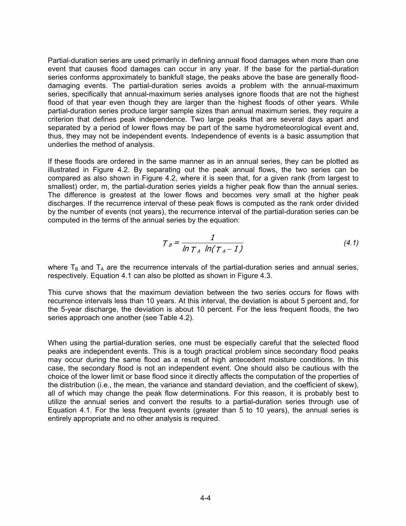
4.2.1 Analysis of Annual and Partial-Duration Series The most common arrangement of hydrologic data is by magnitude of the annual peak discharge. This arrangement is called an annual series. As an example of an annual series, 29 annual peak discharges for Mono Creek near Vermilion Valley, California, are listed in Table 4.1. Another method used in flood data arrangement is the partial-duration series. This procedure uses all peak flows above some base value. For example, the partial-duration series may consider all flows above the discharge of approximately bankfull stage. The USGS sets the base for the partial-duration series so that approximately three peak flows, on average, exceed the base each year. Over a 20-year period of record, this may yield 60 or more floods compared to 20 floods in the annual series. The record contains both annual peaks and partial-duration peaks for unregulated watersheds. Figure 4.1 illustrates a portion of the record for Mono Creek containing both the highest annual floods and other large secondary floods.

4-3

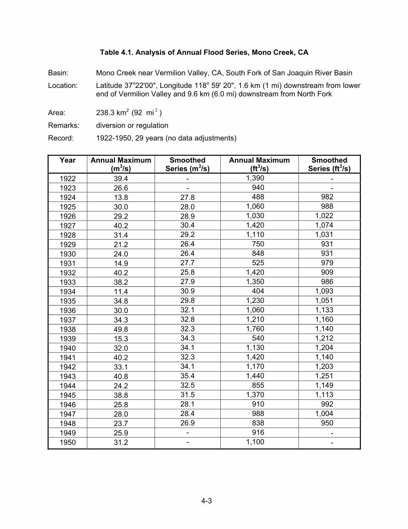
Table 4.1. Analysis of Annual Flood Series, Mono Creek, CA Basin: Mono Creek near Vermilion Valley, CA, South Fork of San Joaquin River Basin

Location: Latitude 37o22'00", Longitude 118o 59' 20", 1.6 km (1 mi) downstream from lower end of Vermilion Valley and 9.6 km (6.0 mi) downstream from North Fork

Area: 238.3 km2 (92 mi 2 )

Remarks: diversion or regulation

Record: 1922-1950, 29 years (no data adjustments)

Year Annual Maximum

(m3/s) Smoothed

Series (m3/s) Annual Maximum

(ft3/s) Smoothed

Series (ft3/s) 1922

39.4

- 1,390

-

1923

26.6

- 940

- 1924

13.8

27.8 488 982

1925

30.0

28.0 1,060 988 1926

29.2

28.9 1,030 1,022

1927

40.2 30.4 1,420 1,074 1928

31.4 29.2 1,110 1,031

1929

21.2 26.4 750 931 1930

24.0 26.4 848 931

1931

14.9 27.7 525 979 1932

40.2 25.8 1,420 909

1933

38.2 27.9 1,350 986 1934

11.4 30.9 404 1,093

1935

34.8 29.8 1,230 1,051 1936

30.0 32.1 1,060 1,133

1937

34.3 32.8 1,210 1,160 1938

49.8 32.3 1,760 1,140

1939

15.3 34.3 540 1,212 1940

32.0 34.1 1,130 1,204

1941

40.2 32.3 1,420 1,140 1942

33.1 34.1 1,170 1,203

1943

40.8 35.4 1,440 1,251 1944

24.2 32.5 855 1,149

1945

38.8 31.5 1,370 1,113 1946

25.8 28.1 910 992

1947

28.0 28.4 988 1,004 1948

23.7 26.9 838 950

1949

25.9 - 916

- 1950

31.2 - 1,100

-

4-4

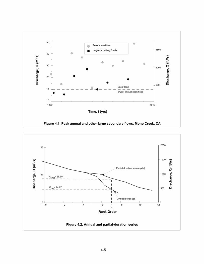
Partial-duration series are used primarily in defining annual flood damages when more than one event that causes flood damages can occur in any year. If the base for the partial-duration series conforms approximately to bankfull stage, the peaks above the base are generally flood-damaging events. The partial-duration series avoids a problem with the annual-maximum series, specifically that annual-maximum series analyses ignore floods that are not the highest flood of that year even though they are larger than the highest floods of other years. While partial-duration series produce larger sample sizes than annual maximum series, they require a criterion that defines peak independence. Two large peaks that are several days apart and separated by a period of lower flows may be part of the same hydrometeorological event and, thus, they may not be independent events. Independence of events is a basic assumption that underlies the method of analysis. If these floods are ordered in the same manner as in an annual series, they can be plotted as illustrated in Figure 4.2. By separating out the peak annual flows, the two series can be compared as also shown in Figure 4.2, where it is seen that, for a given rank (from largest to smallest) order, m, the partial-duration series yields a higher peak flow than the annual series. The difference is greatest at the lower flows and becomes very small at the higher peak discharges. If the recurrence interval of these peak flows is computed as the rank order divided by the number of events (not years), the recurrence interval of the partial-duration series can be computed in the terms of the annual series by the equation:

)1 T(ln T ln

1 = TAA

B − (4.1)

where TB and TA are the recurrence intervals of the partial-duration series and annual series, respectively. Equation 4.1 can also be plotted as shown in Figure 4.3. This curve shows that the maximum deviation between the two series occurs for flows with recurrence intervals less than 10 years. At this interval, the deviation is about 5 percent and, for the 5-year discharge, the deviation is about 10 percent. For the less frequent floods, the two series approach one another (see Table 4.2). When using the partial-duration series, one must be especially careful that the selected flood peaks are independent events. This is a tough practical problem since secondary flood peaks may occur during the same flood as a result of high antecedent moisture conditions. In this case, the secondary flood is not an independent event. One should also be cautious with the choice of the lower limit or base flood since it directly affects the computation of the properties of the distribution (i.e., the mean, the variance and standard deviation, and the coefficient of skew), all of which may change the peak flow determinations. For this reason, it is probably best to utilize the annual series and convert the results to a partial-duration series through use of Equation 4.1. For the less frequent events (greater than 5 to 10 years), the annual series is entirely appropriate and no other analysis is required.

4-5

1930 1940

0

10

20

30

40

50

Time, t (yrs)

Peak annual flow

Large secondary floods

Base flood

lowest annual peak flood

Dis

char

ge, Q

(m3 /s

)

Dis

char

ge, Q

(ft3

/s)

500

1500

1000

Figure 4.1. Peak annual and other large secondary flows, Mono Creek, CA

0 2 4 6 8 10

500

0

28

56

m

Q pds= 26.90

Q as= 14.87

Partial-duration series (pds)

Annual series (as)

Dis

char

ge, Q

(m3 /s

)

012

1000

1500

2000

Dis

char

ge, Q

(ft3

/s)

Rank Order

Figure 4.2. Annual and partial-duration series

4-6

Table 4.2. Comparison of Annual and Partial-Duration Curves

Number of Years Flow is Exceeded per Hundred Years (from Beard, 1962)

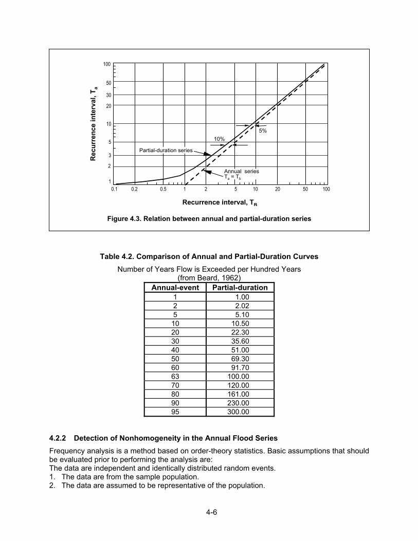
Annual-event Partial-duration 1 1.00 2 2.02 5 5.10 10 10.50 20 22.30 30 35.60 40 51.00 50 69.30 60 91.70 63 100.00 70 120.00 80 161.00 90 230.00 95 300.00

4.2.2 Detection of Nonhomogeneity in the Annual Flood Series Frequency analysis is a method based on order-theory statistics. Basic assumptions that should be evaluated prior to performing the analysis are: The data are independent and identically distributed random events. 1. The data are from the sample population. 2. The data are assumed to be representative of the population.

0.1 0.2 0.5 1 2 5 10 20 50 1001

2

3

5

10

20

30

50

100

Recurrence interval, TB

5%10%

Rec

urre

nce

inte

rval

, Ta

Partial-duration series

Annual seriesTa = Tb

Figure 4.3. Relation between annual and partial-duration series

4-7

3. The process generating these events is stationary with respect to time. Obviously, using a frequency analysis assumes that no measurement or computational errors were made. When analyzing a set of data, the validity of the four assumptions can be statistically evaluated using tests such as the following:

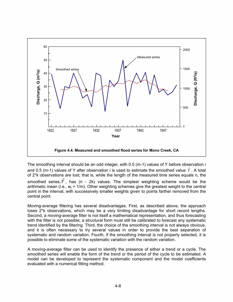
• Runs test for randomness • Mann-Whitney U test for homogeneity • Kendall test for trend • Spearman rank-order correlation coefficient for trend The Kendall test is described by Hirsch, et al. (1982). The other tests are described in the British Flood Studies Report (National Environmental Research Council, 1975) and in the documentation for the Canadian flood-frequency program (Pilon and Harvey, 1992). A work group for revising USGS Bulletin 17B (1982) is currently writing a report that documents and illustrates these tests. Another way to arrange data is according to their time of occurrence. Such an arrangement is called a time series. As an example of a time series, the same 29 years of data presented in Table 4.1 are arranged according to year of occurrence rather than magnitude and plotted in Figure 4.4. This time series shows the temporal variation of the data and is an important step in data analysis. The analysis of time variations is called trend analysis and there are several methods that are used in trend analysis. The two most commonly used in hydrologic analysis are the moving-average method and the methods of curve fitting. A major difference between the moving-average method and curve fitting is that the moving-average method does not provide a mathematical equation for making estimates. It only provides a tabular or graphical summary from which a trend can be subjectively assessed. Curve fitting can provide an equation that can be used to make estimates. The various methods of curve fitting are discussed in more detail by Sanders (1980) and McCuen (1993). The method of moving averages is presented here. Moving-average filtering reduces the effects of random variations. The method is based on the premise that the systematic component of a time series exhibits autocorrelation (i.e., correlation between nearby measurements) while the random fluctuations are not autocorrelated. Therefore, the averaging of adjacent measurements will eliminate the random fluctuations, with the result converging to a qualitative description of any systematic trend that is present in the data. In general, the moving-average computation uses a weighted average of adjacent observations to produce a new time series that consists of the systematic trend. Given a time series Yi, the filtered series iY is derived by:

k)-(n2),...,+(k1),+(k = i for Yw = Y 1-j+k-ij

m

1=ji ∑ (4.2)

where, m = the number of observations used to compute the filtered value (i.e., the smoothing

interval) wj = the weight applied to value j of the series Y.

4-8

The smoothing interval should be an odd integer, with 0.5 (m-1) values of Y before observation i and 0.5 (m-1) values of Y after observation i is used to estimate the smoothed value Y . A total of 2*k observations are lost; that is, while the length of the measured time series equals n, the smoothed series,Y , has (n - 2k) values. The simplest weighting scheme would be the arithmetic mean (i.e., wj = 1/m). Other weighting schemes give the greatest weight to the central point in the interval, with successively smaller weights given to points farther removed from the central point. Moving-average filtering has several disadvantages. First, as described above, the approach loses 2*k observations, which may be a very limiting disadvantage for short record lengths. Second, a moving-average filter is not itself a mathematical representation, and thus forecasting with the filter is not possible; a structural form must still be calibrated to forecast any systematic trend identified by the filtering. Third, the choice of the smoothing interval is not always obvious, and it is often necessary to try several values in order to provide the best separation of systematic and random variation. Fourth, if the smoothing interval is not properly selected, it is possible to eliminate some of the systematic variation with the random variation. A moving-average filter can be used to identify the presence of either a trend or a cycle. The smoothed series will enable the form of the trend or the period of the cycle to be estimated. A model can be developed to represent the systematic component and the model coefficients evaluated with a numerical fitting method.

1922 1927 1932 1937 1942 19470

10

20

30

40

50

60

Year

Smoothed series

Measured series

Dis

char

ge, Q

(ft3

/s)

Dis

char

ge, Q

(m3 /s

)

500

1000

1500

2000

Figure 4.4. Measured and smoothed flood series for Mono Creek, CA

4-9

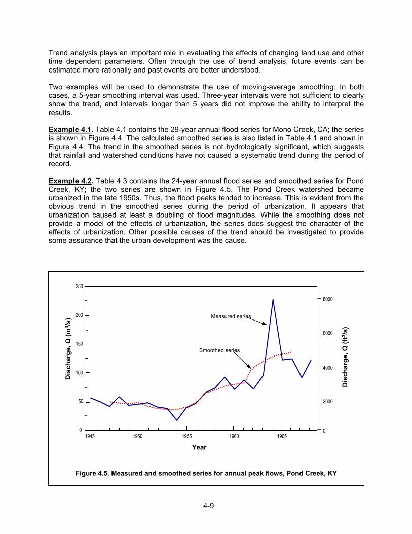
Trend analysis plays an important role in evaluating the effects of changing land use and other time dependent parameters. Often through the use of trend analysis, future events can be estimated more rationally and past events are better understood. Two examples will be used to demonstrate the use of moving-average smoothing. In both cases, a 5-year smoothing interval was used. Three-year intervals were not sufficient to clearly show the trend, and intervals longer than 5 years did not improve the ability to interpret the results.

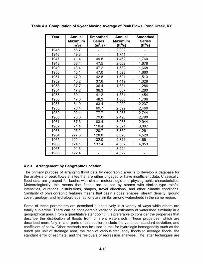
Example 4.1. Table 4.1 contains the 29-year annual flood series for Mono Creek, CA; the series is shown in Figure 4.4. The calculated smoothed series is also listed in Table 4.1 and shown in Figure 4.4. The trend in the smoothed series is not hydrologically significant, which suggests that rainfall and watershed conditions have not caused a systematic trend during the period of record. Example 4.2. Table 4.3 contains the 24-year annual flood series and smoothed series for Pond Creek, KY; the two series are shown in Figure 4.5. The Pond Creek watershed became urbanized in the late 1950s. Thus, the flood peaks tended to increase. This is evident from the obvious trend in the smoothed series during the period of urbanization. It appears that urbanization caused at least a doubling of flood magnitudes. While the smoothing does not provide a model of the effects of urbanization, the series does suggest the character of the effects of urbanization. Other possible causes of the trend should be investigated to provide some assurance that the urban development was the cause.

1945 1950 1955 1960 19650

50

100

150

200

250

Year

Measured series

Smoothed series

0

Dis

char

ge, Q

(ft3

/s)

Dis

char

ge, Q

(m3 /s

)

2000

4000

6000

8000

Figure 4.5. Measured and smoothed series for annual peak flows, Pond Creek, KY

4-10

Table 4.3. Computation of 5-year Moving Average of Peak Flows, Pond Creek, KY

Year Annual Maximum

(m3/s)

Smoothed Series (m3/s)

Annual Maximum

(ft3/s)

Smoothed Series (ft3/s)

1945 56.7 - 2,002 - 1946 49.3 - 1,741 - 1947 41.4 49.8 1,462 1,760 1948 58.4 47.5 2,062 1,678 1949 43.4 47.2 1,532 1,668 1950 45.1 47.0 1,593 1,660 1951 47.9 42.8 1,691 1,513 1952 40.2 37.6 1,419 1,328 1953 37.7 36.4 1,331 1,286 1954 17.2 36.3 607 1,280 1955 39.1 41.2 1,381 1,454 1956 47.0 48.3 1,660 1,706 1957 64.9 63.4 2,292 2,237 1958 73.4 69.7 2,592 2,460 1959 92.4 77.7 3,263 2,744 1960 70.6 79.0 2,493 2,790 1961 87.3 83.4 3,083 2,944 1962 71.4 110.4 2,521 3,897 1963 95.2 120.7 3,362 4,261 1964 227.3 128.0 8,026 4,520 1965 122.1 132.0 4,311 4,661 1966 124.1 137.4 4,382 4,853 1967 91.3 - 3,224 - 1968 122.4 - 4,322 -

4.2.3 Arrangement by Geographic Location The primary purpose of arranging flood data by geographic area is to develop a database for the analysis of peak flows at sites that are either ungaged or have insufficient data. Classically, flood data are grouped for basins with similar meteorologic and physiographic characteristics. Meteorologically, this means that floods are caused by storms with similar type rainfall intensities, durations, distributions, shapes, travel directions, and other climatic conditions. Similarity of physiographic features means that basin slopes, shapes, stream density, ground cover, geology, and hydrologic abstractions are similar among watersheds in the same region. Some of these parameters are described quantitatively in a variety of ways while others are totally subjective. There can be considerable variation in estimates of watershed similarity in a geographical area. From a quantitative standpoint, it is preferable to consider the properties that describe the distribution of floods from different watersheds. These properties, which are described more fully in later parts of this section, include the variance, standard deviation, and coefficient of skew. Other methods can be used to test for hydrologic homogeneity such as the runoff per unit of drainage area, the ratio of various frequency floods to average floods, the standard error of estimate, and the residuals of regression analyses. The latter techniques are

4-11

typical of those used to establish geographic areas for regional regression equations and other regional procedures for peak flow estimates.

4.2.4 Probability Concepts The statistical analysis of repeated observations of an event (e.g., observations of peak annual flows) is based on the laws of probability. The probability of exceedence of a single peak flow, QA, is approximated by the relative number of exceedences of QA after a long series of observations, i.e.,

large)(if nsobservatio of No.

magnitudefloodsomeofsexceedence of No. = nn = )Q(P 1

Ar (4.3)

where, n1 = the frequency n1/n = relative frequency of QA. Most people have an intuitive grasp of the concept of probability. They know that if a coin is tossed, there is an equal probability that a head or a tail will result. They know this because there are only two possible outcomes and that each is equally likely. Again, relying on past experience or intuition, when a fair die is tossed, there are six equally likely outcomes, any of the numbers 1, 2, 3, 4, 5, or 6. Each has a probability of occurrence of 1/6. So the chances that the number 3 will result from a single throw is 1 out of 6. This is fairly straightforward because all of the possible outcomes are known beforehand and the probabilities can be readily quantified. On the other hand, the probability of a nonexceedence (or failure) of an event such as peak flow, QA, is given by:

)Q(P1 = nn1 =

nnn = )Q (notP Ar

11Ar −−

− (4.4)

Combining Equations 4.3 and 4.4 yields: 1 = )Q (notP)Q(P ArAr + (4.5) or the probability of an event being exceeded is between 0 and 1 (i.e., 0 ≤ Pr(QA) ≤ 1). If an event is certain to occur, it has a probability of 1, and if it cannot occur at all, it has a probability of 0. Given two independent flows, QA and QB, the probability of the successive exceedence of both QA and QB is given by: )Q(P )Q(P = )Q and Q(P BrArBAr (4.6) If the exceedence of a flow QA excludes the exceedence of another flow Q2, the two events are said to be mutually exclusive. For mutually exclusive events, the probability of exceedence of either QA or QB is given by: )Q(P + )Q(P = )Q or Q(P BrArBAr (4.7)

4-12

4.2.5 Return Period If the exceedence probability of a given annual peak flow or its relative frequency determined from Equation 4.3 is 0.2, this means that there is a 20 percent chance that this flood, over a long period of time, will be exceeded in any one year. Stated another way, this flood will be exceeded on an average of once every 5 years. That time interval is called the return period, recurrence interval, or exceedence frequency. The return period, Tr, is related to the probability of exceedence by:

)Q(P

1 = TAr

r (4.8)

The designer is cautioned to remember that a flood with a return period of 5 years does not mean this flood will occur once every 5 years. As noted, the flood has a 20 percent probability of being exceeded in any year, and there is no preclusion of the 5-year flood being exceeded in several consecutive years. Two 5-year floods can occur in two consecutive years; there is also a probability that a 5-year flood may not be exceeded in a 10-year period. The same is true for any flood of specified return period.

4.2.6 Estimation of Parameters Flood frequency analysis uses sample information to fit a population, which is a probability distribution. These distributions have parameters that must be estimated in order to make probability statements about the likelihood of future flood magnitudes. A number of methods for estimating the parameters are available. USGS Bulletin 17B (1982) uses the method of moments, which is just one of the parameter-estimation methods. The method of maximum likelihood is a second method. The method of moments equates the moments of the sample flood record to the moments of the population distribution, which yields equations for estimating the parameters of the population as a function of the sample moments. As an example, if the population is assumed to follow distribution f(x), then the sample mean (X) could be related to the definition of the population mean (µ):

(x)dxfx = X ∫∞

∞−

(4.9)

and the sample variance (S2) could be related to the definition of the population variance (σ2):

f(x)dx) (X = S 22 µ−∫∞

∞−

(4.10)

Since f(x) is a function that includes the parameters (µ and σ2), the solution of Equations 4.9 and 4.10 will be expressions that relate X and S2 to the parameters µ and σ2. While maximum likelihood estimation (MLE) is not used in USGS Bulletin 17B (1982) and it is more involved than the method of moments, it is instructive to put MLE in perspective. MLE defines a likelihood function that expresses the probability of obtaining the population

4-13

parameters given that the measured flood record has occurred. For example, if µ and σ are the population parameters and the flood record X contains N events, the likelihood function is:

),|(Xf = )X., . ,.X,X|,L( i

N

N211= i

σµσµ Π (4.11)

where f(XI |µ, σ) is the probability distribution of X as a function of the parameters. The solution of Equation 4.11 will yield expressions for estimating µ and σ from the flood record X.

4.2.7 Frequency Analysis Concepts Future floods cannot be predicted with certainty. Therefore, their magnitude and frequency are treated using probability concepts. To do this, a sample of flood magnitudes are obtained and analyzed for the purpose of estimating a population that can be used to represent flooding at that location. The assumed population is then used in making projections of the magnitude and frequency of floods. It is important to recognize that the population is estimated from sample information and that the assumed population, not the sample, is then used for making statements about the likelihood of future flooding. The purpose of this section is to introduce concepts that are important in analyzing sample flood data in order to identify a probability distribution that can represent the occurrence of flooding.

4.2.7.1 Frequency Histograms

Frequency distributions are used to facilitate an analysis of sample data. A frequency distribution, which is sometimes presented as a histogram, is an arrangement of data by classes or categories with associated frequencies of each class. The frequency distribution shows the magnitude of past events for certain ranges of the variable. Sample probabilities can also be computed by dividing the frequencies of each interval by the sample size. A frequency distribution or histogram is constructed by first examining the range of magnitudes (i.e., the difference between the largest and the smallest floods) and dividing this range into a number of conveniently sized groups, usually between 5 and 20. These groups are called class intervals. The size of the class interval is simply the range divided by the number of class intervals selected. There is no precise rule concerning the number of class intervals to select, but the following guidelines may be helpful: 1. The class intervals should not overlap, and there should be no gaps between the bounds of

the intervals. 2. The number of class intervals should be chosen so that most class intervals have at least

one event. 3. It is preferable that the class intervals are of equal width. 4. It is also preferable for most class intervals to have at least five occurrences; this may not be

practical for the first and last intervals. Example 4.3. Using these rules, the discharges for Mono Creek listed in Table 4.1 are placed into a frequency histogram using class intervals of 5 m3/s (SI) and 200 ft3/s (CU units) (see Table 4.4). These data can also be represented graphically by a frequency histogram as shown

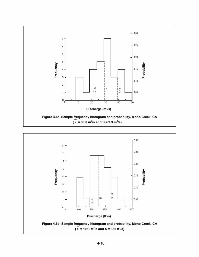
4-14

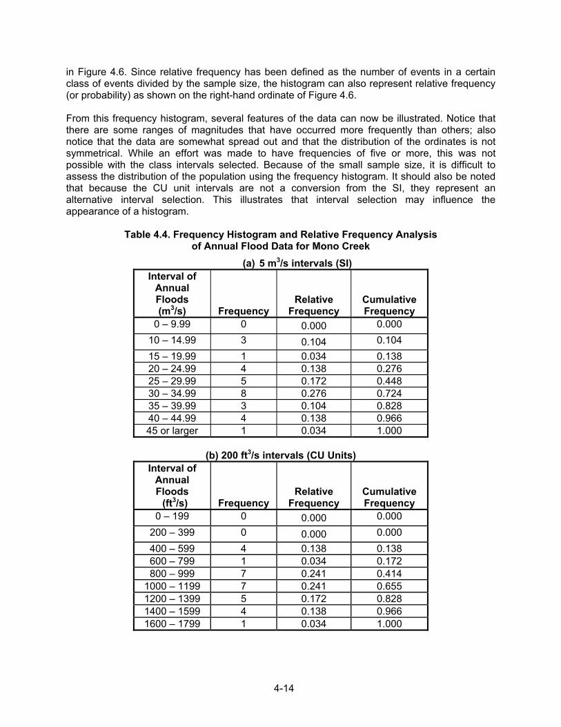
in Figure 4.6. Since relative frequency has been defined as the number of events in a certain class of events divided by the sample size, the histogram can also represent relative frequency (or probability) as shown on the right-hand ordinate of Figure 4.6. From this frequency histogram, several features of the data can now be illustrated. Notice that there are some ranges of magnitudes that have occurred more frequently than others; also notice that the data are somewhat spread out and that the distribution of the ordinates is not symmetrical. While an effort was made to have frequencies of five or more, this was not possible with the class intervals selected. Because of the small sample size, it is difficult to assess the distribution of the population using the frequency histogram. It should also be noted that because the CU unit intervals are not a conversion from the SI, they represent an alternative interval selection. This illustrates that interval selection may influence the appearance of a histogram.

Table 4.4. Frequency Histogram and Relative Frequency Analysis of Annual Flood Data for Mono Creek

(a) 5 m3/s intervals (SI) Interval of

Annual Floods (m3/s) Frequency

Relative Frequency

Cumulative Frequency

0 – 9.99 0 0.000 0.000 10 – 14.99 3 0.104 0.104 15 – 19.99 1 0.034 0.138 20 – 24.99 4 0.138 0.276 25 – 29.99 5 0.172 0.448 30 – 34.99 8 0.276 0.724 35 – 39.99 3 0.104 0.828 40 – 44.99 4 0.138 0.966 45 or larger 1 0.034 1.000

(b) 200 ft3/s intervals (CU Units)

Interval of Annual Floods (ft3/s) Frequency

Relative Frequency

Cumulative Frequency

0 – 199 0 0.000 0.000 200 – 399 0 0.000 0.000 400 – 599 4 0.138 0.138 600 – 799 1 0.034 0.172 800 – 999 7 0.241 0.414

1000 – 1199 7 0.241 0.655 1200 – 1399 5 0.172 0.828 1400 – 1599 4 0.138 0.966 1600 – 1799 1 0.034 1.000

4-15

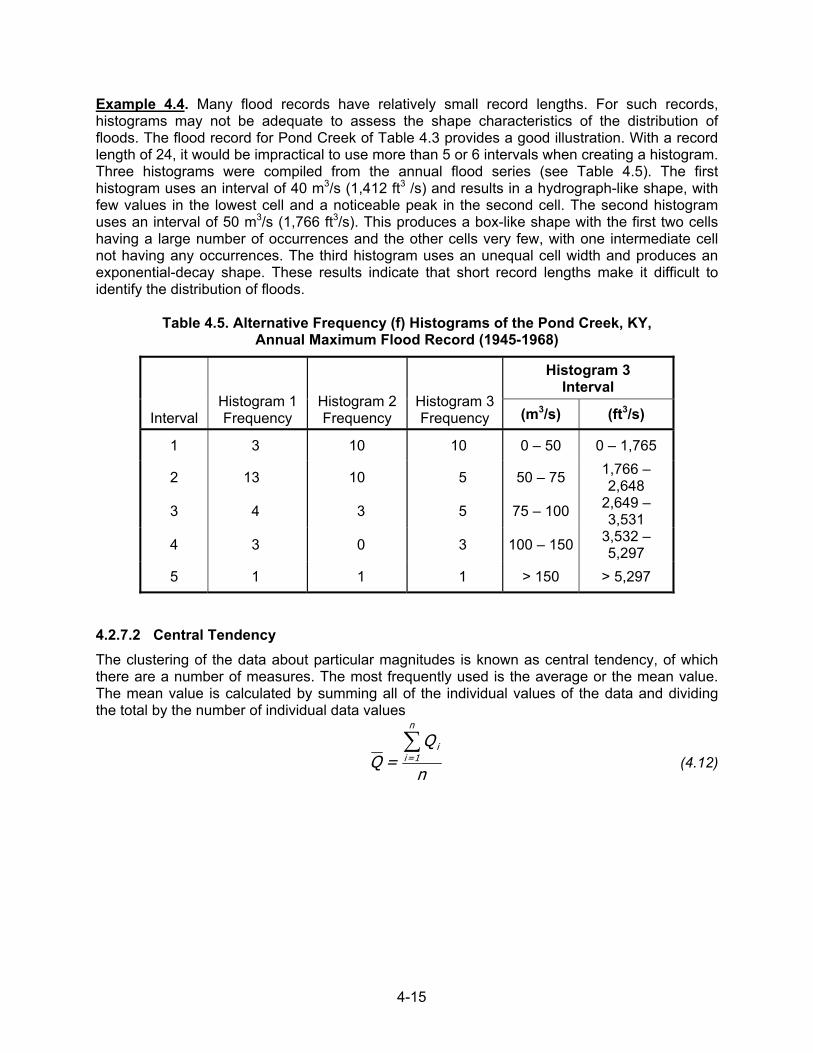
Example 4.4. Many flood records have relatively small record lengths. For such records, histograms may not be adequate to assess the shape characteristics of the distribution of floods. The flood record for Pond Creek of Table 4.3 provides a good illustration. With a record length of 24, it would be impractical to use more than 5 or 6 intervals when creating a histogram. Three histograms were compiled from the annual flood series (see Table 4.5). The first histogram uses an interval of 40 m3/s (1,412 ft3 /s) and results in a hydrograph-like shape, with few values in the lowest cell and a noticeable peak in the second cell. The second histogram uses an interval of 50 m3/s (1,766 ft3/s). This produces a box-like shape with the first two cells having a large number of occurrences and the other cells very few, with one intermediate cell not having any occurrences. The third histogram uses an unequal cell width and produces an exponential-decay shape. These results indicate that short record lengths make it difficult to identify the distribution of floods.

Table 4.5. Alternative Frequency (f) Histograms of the Pond Creek, KY, Annual Maximum Flood Record (1945-1968)

Histogram 3 Interval

Interval Histogram 1 Frequency

Histogram 2 Frequency

Histogram 3 Frequency (m3/s) (ft3/s)

1 3 10 10 0 – 50 0 – 1,765

2 13 10 5 50 – 75 1,766 – 2,648

3 4 3 5 75 – 100 2,649 – 3,531

4 3 0 3 100 – 150 3,532 – 5,297

5 1 1 1 > 150 > 5,297

4.2.7.2 Central Tendency The clustering of the data about particular magnitudes is known as central tendency, of which there are a number of measures. The most frequently used is the average or the mean value. The mean value is calculated by summing all of the individual values of the data and dividing the total by the number of individual data values

n

Q = Q

i

n

1=i∑

(4.12)

4-16

0 400 800 1200 1600 20000

1

2

3

4

5

6

7

8

Discharge (ft³/s)

0.30

0.25

0.20

0.15

0.10

0.05

Freq

uenc

y

Prob

abili

ty

_ X - S

_ X _ X +

S

Figure 4.6b. Sample frequency histogram and probability, Mono Creek, CA ( x = 1060 ft3/s and S = 330 ft3/s)

0 10 20 30 40 500

1

2

3

4

5

6

7

8

Discharge (m³/s)

0.30

0.25

0.20

0.15

0.10

0.05

Freq

uenc

y

Prob

abili

ty

_ X - S _ X

_ X +

S

Figure 4.6a. Sample frequency histogram and probability, Mono Creek, CA ( x = 30.0 m3/s and S = 9.3 m3/s)

4-17

where, Q = average or mean peak. The median, another measure of central tendency, is the value of the middle item when the items are arranged according to magnitude. When there is an even number of items, the median is taken as the average of the two central values. The mode is a third measure of central tendency. The mode is the most frequent or most common value that occurs in a set of data. For continuous variables, such as discharge rates, the mode is defined as the central value of the most frequent class interval.

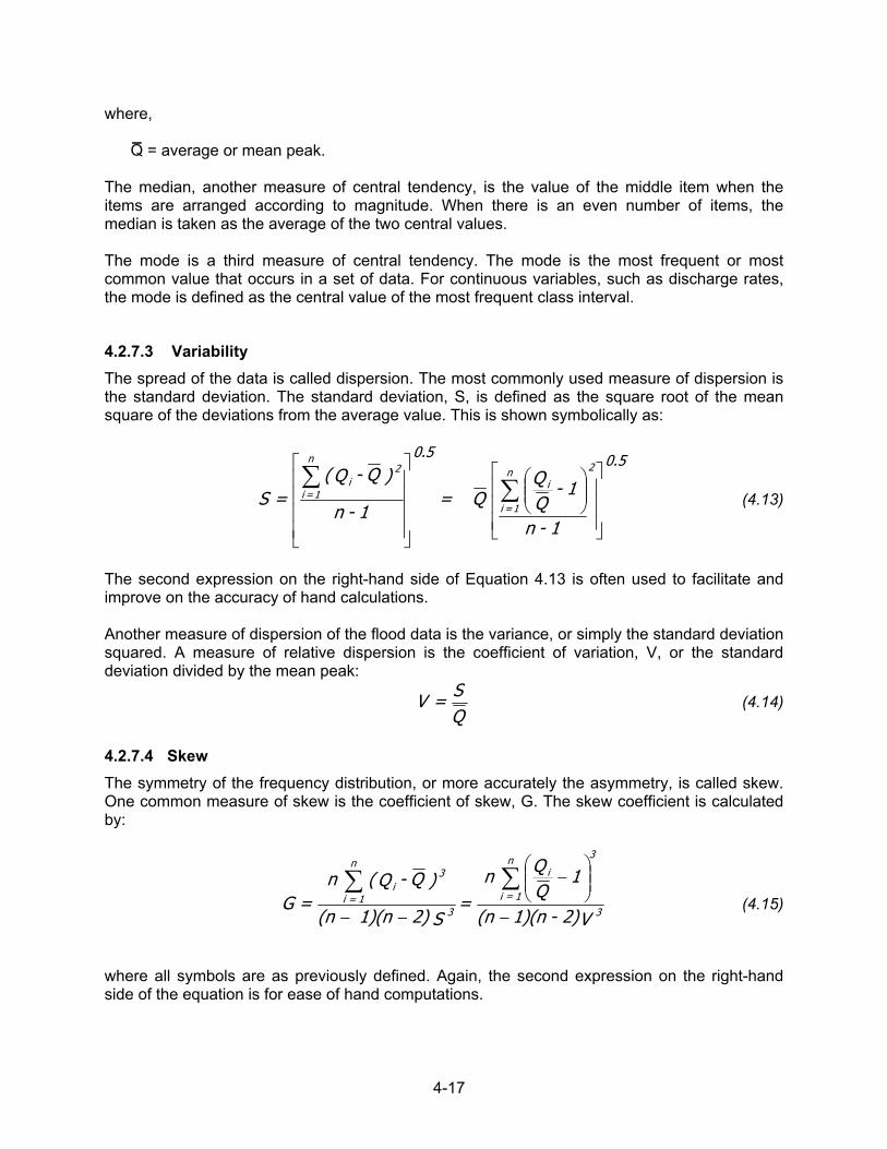
4.2.7.3 Variability The spread of the data is called dispersion. The most commonly used measure of dispersion is the standard deviation. The standard deviation, S, is defined as the square root of the mean square of the deviations from the average value. This is shown symbolically as:

∑∑

1-n

1- QQ Q =

1-n

)Q-Q( = S

in

1=i

22i

n

1=i

0.50.5

(4.13)

The second expression on the right-hand side of Equation 4.13 is often used to facilitate and improve on the accuracy of hand calculations. Another measure of dispersion of the flood data is the variance, or simply the standard deviation squared. A measure of relative dispersion is the coefficient of variation, V, or the standard deviation divided by the mean peak:

QS = V (4.14)

4.2.7.4 Skew The symmetry of the frequency distribution, or more accurately the asymmetry, is called skew. One common measure of skew is the coefficient of skew, G. The skew coefficient is calculated by:

V2) - 1)(n (n

1 QQ n

= S2) 1)(n (n

)Q - Q( n = G 3

in

1 = i

3

3

3i

n

1 = i

−

−

−−

∑∑ (4.15)

where all symbols are as previously defined. Again, the second expression on the right-hand side of the equation is for ease of hand computations.

4-18

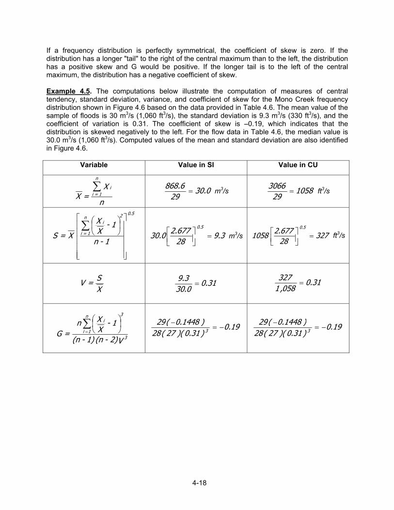
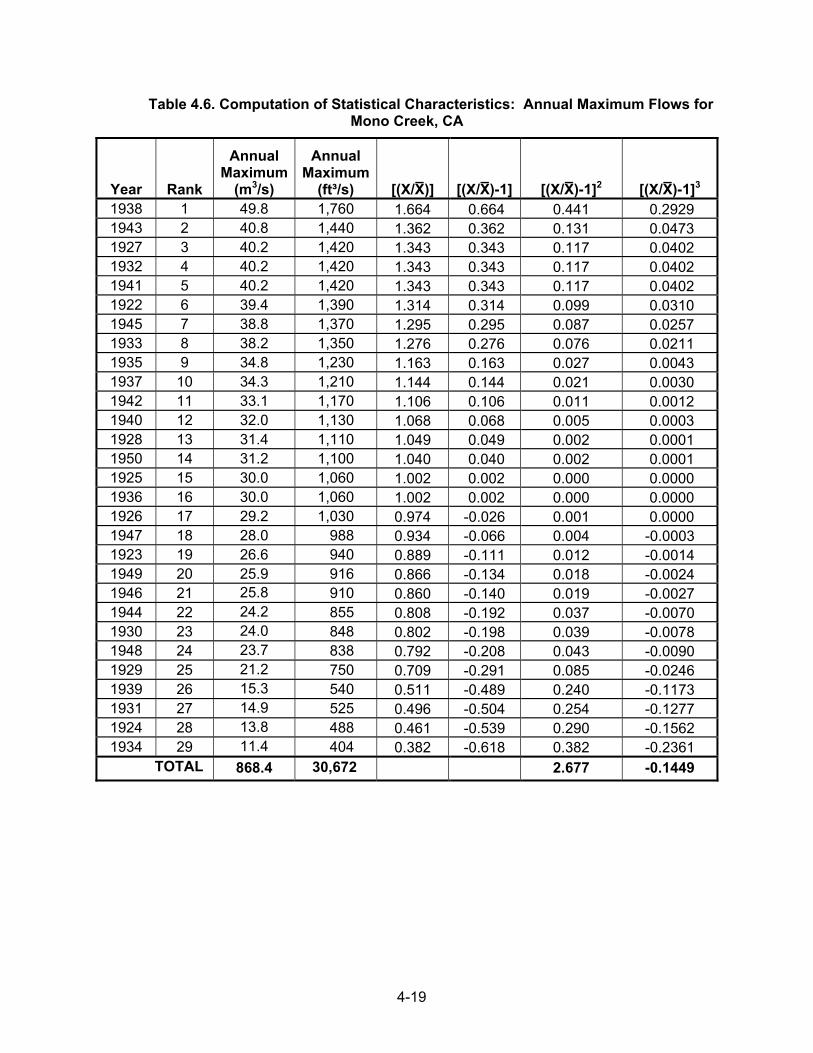
If a frequency distribution is perfectly symmetrical, the coefficient of skew is zero. If the distribution has a longer "tail" to the right of the central maximum than to the left, the distribution has a positive skew and G would be positive. If the longer tail is to the left of the central maximum, the distribution has a negative coefficient of skew. Example 4.5. The computations below illustrate the computation of measures of central tendency, standard deviation, variance, and coefficient of skew for the Mono Creek frequency distribution shown in Figure 4.6 based on the data provided in Table 4.6. The mean value of the sample of floods is 30 m3/s (1,060 ft3/s), the standard deviation is 9.3 m3/s (330 ft3/s), and the coefficient of variation is 0.31. The coefficient of skew is –0.19, which indicates that the distribution is skewed negatively to the left. For the flow data in Table 4.6, the median value is 30.0 m3/s (1,060 ft3/s). Computed values of the mean and standard deviation are also identified in Figure 4.6.

Variable Value in SI Value in CU

n

X = X

i

n

1 = i∑

0.30

296.868

= m3/s 105829

3066= ft3/s

∑1 - n

1 - XX

X = S

in

1 = i

2 0.5

3.928677.20.30

5.0

=

m3/s 327

28677.21058

5.0

=

ft3/s

XS = V 31.0

0.303.9

= 31.0058,1

327=

V2)-(n1)-(n

1-XXn

= G 3

n

1i

i3

∑=

19.0

)31.0)(27(28)1448.0(29

3 −=−

19.0)31.0)(27(28)1448.0(29

3 −=−

4-19

Table 4.6. Computation of Statistical Characteristics: Annual Maximum Flows for Mono Creek, CA

Year Rank

Annual Maximum

(m3/s)

Annual

Maximum(ft³/s)

[(X/X)]

[(X/X)-1]

[(X/X)-1]2

[(X/X)-1]3 1938 1 49.8 1,760

1.664

0.664

0.441

0.2929

1943 2 40.8 1,440

1.362

0.362

0.131

0.0473 1927 3 40.2 1,420

1.343

0.343

0.117

0.0402

1932 4 40.2 1,420

1.343

0.343

0.117

0.0402 1941 5 40.2 1,420

1.343

0.343

0.117

0.0402

1922 6 39.4 1,390

1.314

0.314

0.099

0.0310 1945 7 38.8 1,370

1.295

0.295

0.087

0.0257

1933 8 38.2 1,350

1.276

0.276

0.076

0.0211 1935 9 34.8 1,230

1.163

0.163

0.027

0.0043

1937 10 34.3 1,210

1.144

0.144

0.021

0.0030 1942 11 33.1 1,170

1.106

0.106

0.011

0.0012

1940 12 32.0 1,130

1.068

0.068

0.005

0.0003 1928 13 31.4 1,110

1.049

0.049

0.002

0.0001

1950 14 31.2 1,100

1.040

0.040

0.002

0.0001 1925 15 30.0 1,060

1.002

0.002

0.000

0.0000

1936 16 30.0 1,060

1.002

0.002

0.000

0.0000 1926 17 29.2 1,030

0.974

-0.026

0.001

0.0000

1947 18 28.0 988

0.934

-0.066

0.004

-0.0003 1923 19 26.6 940

0.889

-0.111

0.012

-0.0014

1949 20 25.9 916

0.866

-0.134

0.018

-0.0024 1946 21 25.8 910

0.860

-0.140

0.019

-0.0027

1944 22 24.2 855

0.808

-0.192

0.037

-0.0070 1930 23 24.0 848

0.802

-0.198

0.039

-0.0078

1948 24 23.7 838

0.792

-0.208

0.043

-0.0090 1929 25 21.2 750

0.709

-0.291

0.085

-0.0246

1939 26 15.3 540

0.511

-0.489

0.240

-0.1173 1931 27 14.9 525

0.496

-0.504

0.254

-0.1277

1924 28 13.8 488

0.461

-0.539

0.290

-0.1562 1934 29 11.4 404

0.382

-0.618

0.382

-0.2361

TOTAL

868.4 30,672

2.677

-0.1449

4-20

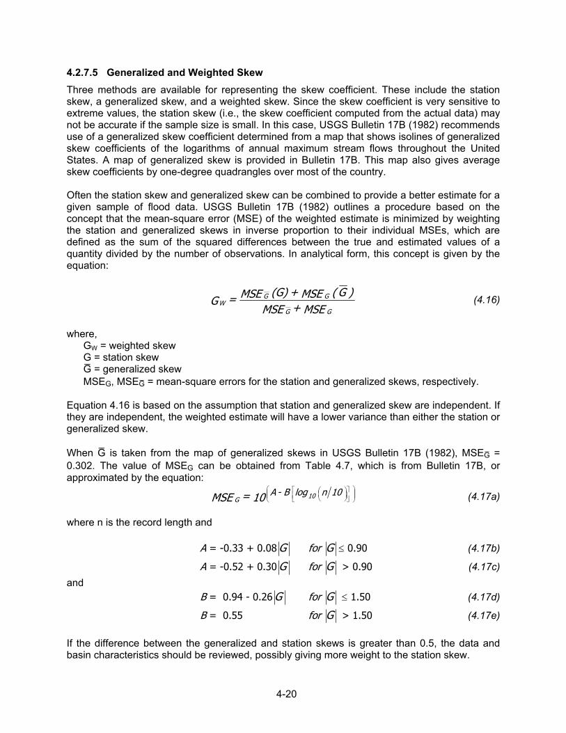
4.2.7.5 Generalized and Weighted Skew Three methods are available for representing the skew coefficient. These include the station skew, a generalized skew, and a weighted skew. Since the skew coefficient is very sensitive to extreme values, the station skew (i.e., the skew coefficient computed from the actual data) may not be accurate if the sample size is small. In this case, USGS Bulletin 17B (1982) recommends use of a generalized skew coefficient determined from a map that shows isolines of generalized skew coefficients of the logarithms of annual maximum stream flows throughout the United States. A map of generalized skew is provided in Bulletin 17B. This map also gives average skew coefficients by one-degree quadrangles over most of the country. Often the station skew and generalized skew can be combined to provide a better estimate for a given sample of flood data. USGS Bulletin 17B (1982) outlines a procedure based on the concept that the mean-square error (MSE) of the weighted estimate is minimized by weighting the station and generalized skews in inverse proportion to their individual MSEs, which are defined as the sum of the squared differences between the true and estimated values of a quantity divided by the number of observations. In analytical form, this concept is given by the equation:

MSE + MSE

)G( MSE + (G) MSE = GGG

GGW (4.16)

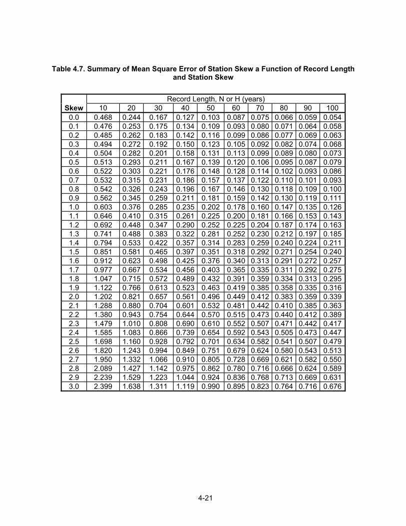
where, GW = weighted skew G = station skew G = generalized skew MSEG, MSEG = mean-square errors for the station and generalized skews, respectively. Equation 4.16 is based on the assumption that station and generalized skew are independent. If they are independent, the weighted estimate will have a lower variance than either the station or generalized skew. When G is taken from the map of generalized skews in USGS Bulletin 17B (1982), MSEG = 0.302. The value of MSEG can be obtained from Table 4.7, which is from Bulletin 17B, or approximated by the equation:

10 = MSE 10 G

10nlogB -A

(4.17a) where n is the record length and

A = -0.33 + 0.08 G for G ≤ 0.90 (4.17b)

A = -0.52 + 0.30 G for G > 0.90 (4.17c) and

B = 0.94 - 0.26 G for G ≤ 1.50 (4.17d)

B = 0.55 for G > 1.50 (4.17e) If the difference between the generalized and station skews is greater than 0.5, the data and basin characteristics should be reviewed, possibly giving more weight to the station skew.

4-21

Table 4.7. Summary of Mean Square Error of Station Skew a Function of Record Length

and Station Skew

Record Length, N or H (years) Skew 10 20 30 40 50 60 70 80 90 100

0.0 0.468 0.244 0.167 0.127 0.103 0.087 0.075 0.066 0.059 0.0540.1 0.476 0.253 0.175 0.134 0.109 0.093 0.080 0.071 0.064 0.0580.2 0.485 0.262 0.183 0.142 0.116 0.099 0.086 0.077 0.069 0.0630.3 0.494 0.272 0.192 0.150 0.123 0.105 0.092 0.082 0.074 0.0680.4 0.504 0.282 0.201 0.158 0.131 0.113 0.099 0.089 0.080 0.0730.5 0.513 0.293 0.211 0.167 0.139 0.120 0.106 0.095 0.087 0.0790.6 0.522 0.303 0.221 0.176 0.148 0.128 0.114 0.102 0.093 0.0860.7 0.532 0.315 0.231 0.186 0.157 0.137 0.122 0.110 0.101 0.0930.8 0.542 0.326 0.243 0.196 0.167 0.146 0.130 0.118 0.109 0.1000.9 0.562 0.345 0.259 0.211 0.181 0.159 0.142 0.130 0.119 0.1111.0 0.603 0.376 0.285 0.235 0.202 0.178 0.160 0.147 0.135 0.1261.1 0.646 0.410 0.315 0.261 0.225 0.200 0.181 0.166 0.153 0.1431.2 0.692 0.448 0.347 0.290 0.252 0.225 0.204 0.187 0.174 0.1631.3 0.741 0.488 0.383 0.322 0.281 0.252 0.230 0.212 0.197 0.1851.4 0.794 0.533 0.422 0.357 0.314 0.283 0.259 0.240 0.224 0.2111.5 0.851 0.581 0.465 0.397 0.351 0.318 0.292 0.271 0.254 0.2401.6 0.912 0.623 0.498 0.425 0.376 0.340 0.313 0.291 0.272 0.2571.7 0.977 0.667 0.534 0.456 0.403 0.365 0.335 0.311 0.292 0.2751.8 1.047 0.715 0.572 0.489 0.432 0.391 0.359 0.334 0.313 0.2951.9 1.122 0.766 0.613 0.523 0.463 0.419 0.385 0.358 0.335 0.3162.0 1.202 0.821 0.657 0.561 0.496 0.449 0.412 0.383 0.359 0.3392.1 1.288 0.880 0.704 0.601 0.532 0.481 0.442 0.410 0.385 0.3632.2 1.380 0.943 0.754 0.644 0.570 0.515 0.473 0.440 0.412 0.3892.3 1.479 1.010 0.808 0.690 0.610 0.552 0.507 0.471 0.442 0.4172.4 1.585 1.083 0.866 0.739 0.654 0.592 0.543 0.505 0.473 0.4472.5 1.698 1.160 0.928 0.792 0.701 0.634 0.582 0.541 0.507 0.4792.6 1.820 1.243 0.994 0.849 0.751 0.679 0.624 0.580 0.543 0.5132.7 1.950 1.332 1.066 0.910 0.805 0.728 0.669 0.621 0.582 0.5502.8 2.089 1.427 1.142 0.975 0.862 0.780 0.716 0.666 0.624 0.5892.9 2.239 1.529 1.223 1.044 0.924 0.836 0.768 0.713 0.669 0.6313.0 2.399 1.638 1.311 1.119 0.990 0.895 0.823 0.764 0.716 0.676

4-22

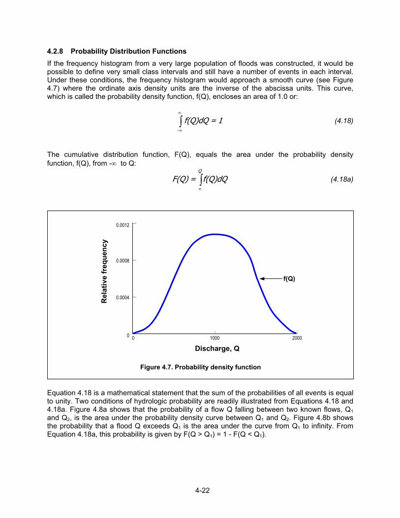
4.2.8 Probability Distribution Functions If the frequency histogram from a very large population of floods was constructed, it would be possible to define very small class intervals and still have a number of events in each interval. Under these conditions, the frequency histogram would approach a smooth curve (see Figure 4.7) where the ordinate axis density units are the inverse of the abscissa units. This curve, which is called the probability density function, f(Q), encloses an area of 1.0 or:

1 = f(Q)dQ -∫∞

∞

(4.18)

The cumulative distribution function, F(Q), equals the area under the probability density function, f(Q), from -∞ to Q:

f(Q)dQ = F(Q)Q

∫∞

(4.18a)

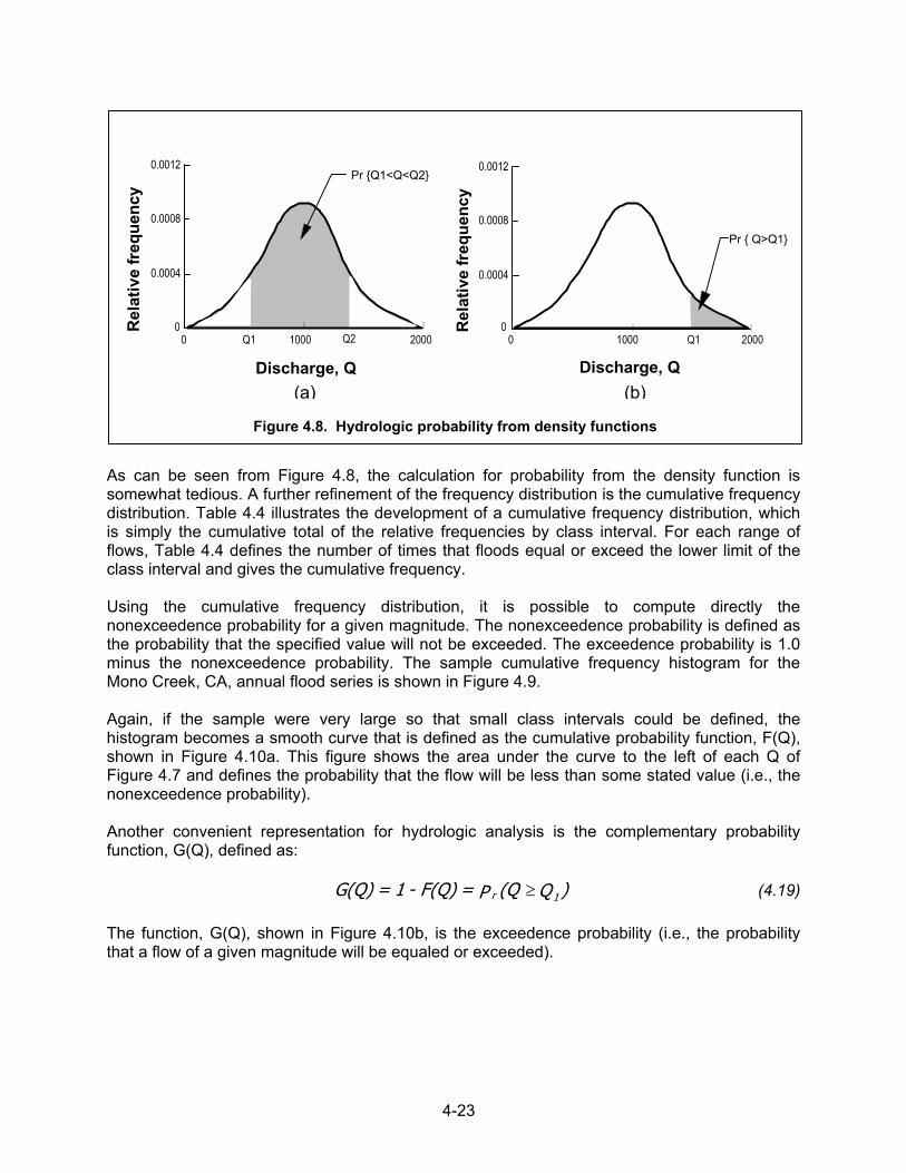
Equation 4.18 is a mathematical statement that the sum of the probabilities of all events is equal to unity. Two conditions of hydrologic probability are readily illustrated from Equations 4.18 and 4.18a. Figure 4.8a shows that the probability of a flow Q falling between two known flows, Q1 and Q2, is the area under the probability density curve between Q1 and Q2. Figure 4.8b shows the probability that a flood Q exceeds Q1 is the area under the curve from Q1 to infinity. From Equation 4.18a, this probability is given by F(Q > Q1) = 1 - F(Q < Q1).

0 1000 20000

0.0004

0.0008

0.0012

Discharge, Q

f(Q)

Rel

ativ

e fr

eque

ncy

Figure 4.7. Probability density function

4-23

As can be seen from Figure 4.8, the calculation for probability from the density function is somewhat tedious. A further refinement of the frequency distribution is the cumulative frequency distribution. Table 4.4 illustrates the development of a cumulative frequency distribution, which is simply the cumulative total of the relative frequencies by class interval. For each range of flows, Table 4.4 defines the number of times that floods equal or exceed the lower limit of the class interval and gives the cumulative frequency. Using the cumulative frequency distribution, it is possible to compute directly the nonexceedence probability for a given magnitude. The nonexceedence probability is defined as the probability that the specified value will not be exceeded. The exceedence probability is 1.0 minus the nonexceedence probability. The sample cumulative frequency histogram for the Mono Creek, CA, annual flood series is shown in Figure 4.9. Again, if the sample were very large so that small class intervals could be defined, the histogram becomes a smooth curve that is defined as the cumulative probability function, F(Q), shown in Figure 4.10a. This figure shows the area under the curve to the left of each Q of Figure 4.7 and defines the probability that the flow will be less than some stated value (i.e., the nonexceedence probability). Another convenient representation for hydrologic analysis is the complementary probability function, G(Q), defined as: )Q (QP = F(Q) - 1 = G(Q) 1r ≥ (4.19)

The function, G(Q), shown in Figure 4.10b, is the exceedence probability (i.e., the probability that a flow of a given magnitude will be equaled or exceeded).

0 1000 20000

0.0004

0.0008

0.0012

Pr { Q>Q1}

0 1000 20000

0.0004

0.0008

0.0012

Discharge, Q

Pr {Q1<Q<Q2}

(b) (a)

Q1 Q2 Q1

Rel

ativ

e fr

eque

ncy

Discharge, Q

Rel

ativ

e fr

eque

ncy

Figure 4.8. Hydrologic probability from density functions

4-24

4.2.9 Plotting Position Formulas When making a flood frequency analysis, it is common to plot both the assumed population and the peak discharges of the sample. To plot the sample values on frequency paper, it is necessary to assign an exceedence probability to each magnitude. A plotting position formula is used for this purpose.

00.0

0.2

0.4

0.6

0.8

1.0

Discharge, Q500 1000 1500 2000

(a) (b)

00.0

0.2

0.4

0.6

0.8

1.0

Discharge, Q

Com

plem

enta

ryC

umul

ativ

e pr

obab

ility

, G (Q

)

Cum

ulat

ive

prob

abili

ty, G

(Q)

500 1000 1500 2000

Figure 4.10. Cumulative and complementary cumulative distribution functions

0 500.0

0.2

0.4

0.6

0.8

1.0

Discharge, Q (m³/s)

Cum

ulat

ive

freq

uenc

y

10 20 30 40

0 500 1000 1500

Discharge, Q (ft3/s)

Figure 4.9. Cumulative frequency histogram, Mono Creek, CA

4-25

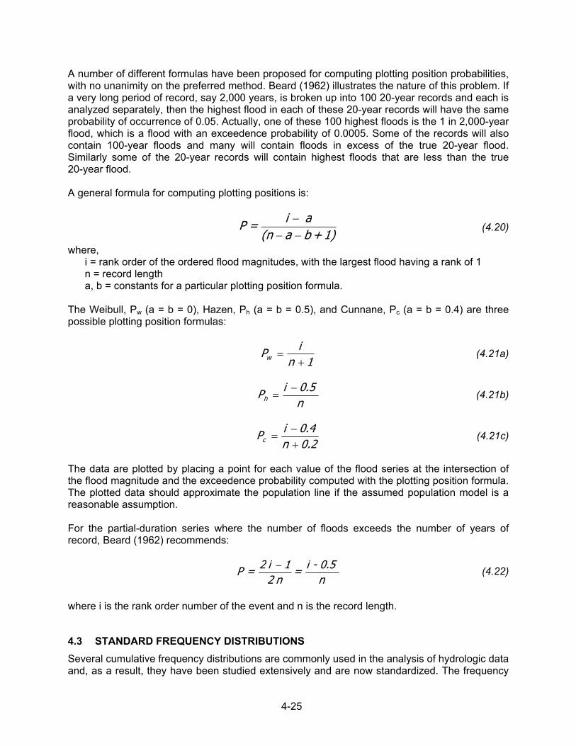
A number of different formulas have been proposed for computing plotting position probabilities, with no unanimity on the preferred method. Beard (1962) illustrates the nature of this problem. If a very long period of record, say 2,000 years, is broken up into 100 20-year records and each is analyzed separately, then the highest flood in each of these 20-year records will have the same probability of occurrence of 0.05. Actually, one of these 100 highest floods is the 1 in 2,000-year flood, which is a flood with an exceedence probability of 0.0005. Some of the records will also contain 100-year floods and many will contain floods in excess of the true 20-year flood. Similarly some of the 20-year records will contain highest floods that are less than the true 20-year flood. A general formula for computing plotting positions is:

1) + b a (n

a i = P−−−

(4.20)

where, i = rank order of the ordered flood magnitudes, with the largest flood having a rank of 1 n = record length a, b = constants for a particular plotting position formula. The Weibull, Pw (a = b = 0), Hazen, Ph (a = b = 0.5), and Cunnane, Pc (a = b = 0.4) are three possible plotting position formulas:

1n

iPw += (4.21a)

n

5.0iPh−

= (4.21b)

2.0n4.0iPc +

−= (4.21c)

The data are plotted by placing a point for each value of the flood series at the intersection of the flood magnitude and the exceedence probability computed with the plotting position formula. The plotted data should approximate the population line if the assumed population model is a reasonable assumption. For the partial-duration series where the number of floods exceeds the number of years of record, Beard (1962) recommends:

n0.5-i =

n21i2 = P − (4.22)

where i is the rank order number of the event and n is the record length.

4.3 STANDARD FREQUENCY DISTRIBUTIONS Several cumulative frequency distributions are commonly used in the analysis of hydrologic data and, as a result, they have been studied extensively and are now standardized. The frequency

4-26

distributions that have been found most useful in hydrologic data analysis are the normal distribution, the log-normal distribution, the Gumbel extreme value distribution, and the log-Pearson Type III distribution. The characteristics and application of each of these distributions will be presented in the following sections.

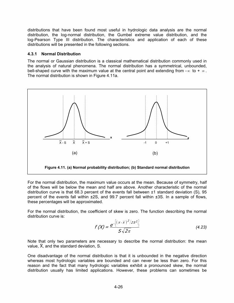
4.3.1 Normal Distribution The normal or Gaussian distribution is a classical mathematical distribution commonly used in the analysis of natural phenomena. The normal distribution has a symmetrical, unbounded, bell-shaped curve with the maximum value at the central point and extending from - ∞ to + ∞ . The normal distribution is shown in Figure 4.11a.

For the normal distribution, the maximum value occurs at the mean. Because of symmetry, half of the flows will be below the mean and half are above. Another characteristic of the normal distribution curve is that 68.3 percent of the events fall between ±1 standard deviation (S), 95 percent of the events fall within ±2S, and 99.7 percent fall within ±3S. In a sample of flows, these percentages will be approximated. For the normal distribution, the coefficient of skew is zero. The function describing the normal distribution curve is:

( )

π2Se = (X)f

22XX S2−

−

(4.23)

Note that only two parameters are necessary to describe the normal distribution: the mean value, X, and the standard deviation, S. One disadvantage of the normal distribution is that it is unbounded in the negative direction whereas most hydrologic variables are bounded and can never be less than zero. For this reason and the fact that many hydrologic variables exhibit a pronounced skew, the normal distribution usually has limited applications. However, these problems can sometimes be

x z0 +1 -1X + S X - S X

(a) (b)

Figure 4.11. (a) Normal probability distribution; (b) Standard normal distribution

4-27

overcome by performing a log transform on the data. Often the logarithms of hydrologic variables are normally distributed.

4.3.1.1 Standard Normal Distribution A special case of the normal distribution of Equation 4.23 is called the standard normal distribution and is represented by the variate z (see Figure 4.11b). The standard normal distribution always has a mean of 0 and a standard deviation of 1. If the random variable X has a normal distribution with mean X and standard deviation S, values of X can be transformed so that they have a standard normal distribution using the following transformation:

S

X - X = z (4.24)

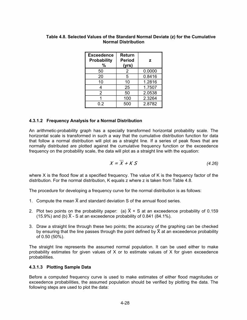
If X, S, and z for a given frequency are known, then the value of X corresponding to the frequency can be computed by algebraic manipulation of Equation 4.24: zS + X = X (4.25) To illustrate, the 10-year event has an exceedence probability of 0.10 or a nonexceedence probability of 0.90. Thus, the corresponding value of z from Table 4.8 is 1.2816. If floods have a normal distribution with a mean of 120 m3/s (4,240 ft3/s) and a standard deviation of 35 m³/s (1,230 ft3/s), the 10-year flood for a normal distribution is computed with Equation 4.25:

Variable Value in SI Value in CU zS + X = X

/sm 165 = 1.2816(35) + 120 = 3 /sft 165 = 0)1.2816(123 + 4240 = 3

Similarly, the frequency of a flood of 181 m3/s (6,390 ft3/s) can be estimated using the transform of Equation 4.24:

Variable Value in SI Value in CU

Sxxz −

= 75.135

120181=

−= 75.1

123042406390

=−

=

From Table 4.8, this corresponds to an exceedence probability of 4 percent, which is the 25-year flood.

4-28

Table 4.8. Selected Values of the Standard Normal Deviate (z) for the Cumulative

Normal Distribution

Exceedence Probability

%

Return Period (yrs)

z

50 2 0.0000 20 5 0.8416 10 10 1.2816 4 25 1.7507 2 50 2.0538 1 100 2.3264

0.2 500 2.8782

4.3.1.2 Frequency Analysis for a Normal Distribution

An arithmetic-probability graph has a specially transformed horizontal probability scale. The horizontal scale is transformed in such a way that the cumulative distribution function for data that follow a normal distribution will plot as a straight line. If a series of peak flows that are normally distributed are plotted against the cumulative frequency function or the exceedence frequency on the probability scale, the data will plot as a straight line with the equation:

SK + X = X (4.26)

where X is the flood flow at a specified frequency. The value of K is the frequency factor of the distribution. For the normal distribution, K equals z where z is taken from Table 4.8. The procedure for developing a frequency curve for the normal distribution is as follows: 1. Compute the mean X and standard deviation S of the annual flood series. 2. Plot two points on the probability paper: (a) X + S at an exceedence probability of 0.159

(15.9%) and (b) X - S at an exceedence probability of 0.841 (84.1%). 3. Draw a straight line through these two points; the accuracy of the graphing can be checked

by ensuring that the line passes through the point defined by X at an exceedence probability of 0.50 (50%).

The straight line represents the assumed normal population. It can be used either to make probability estimates for given values of X or to estimate values of X for given exceedence probabilities.

4.3.1.3 Plotting Sample Data

Before a computed frequency curve is used to make estimates of either flood magnitudes or exceedence probabilities, the assumed population should be verified by plotting the data. The following steps are used to plot the data:

4-29

1. Rank the flood series in descending order, with the largest flood having a rank of 1 and the

smallest flood having a rank of n. 2. Use the rank (i) with a plotting position formula such as Equation 4.21, and compute the

plotting probabilities for each flood. 3. Plot the magnitude X against the corresponding plotting probability. If the data follow the trend of the assumed population line, one usually assumes that the data are normally distributed. It is not uncommon for the sample points on the upper and lower ends to deviate from the straight line. Deciding whether or not to accept the computed straight line as the population is based on experience rather than an objective criterion.

4.3.1.4 Estimation with the Frequency Curve

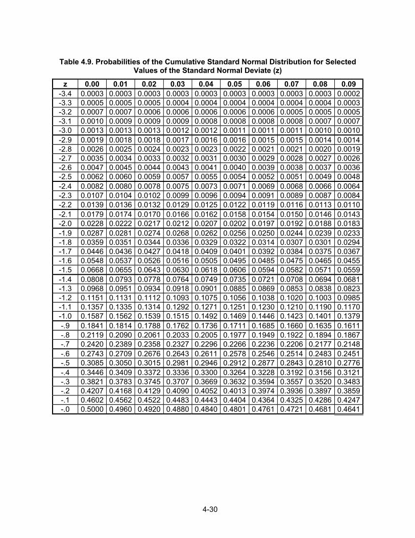
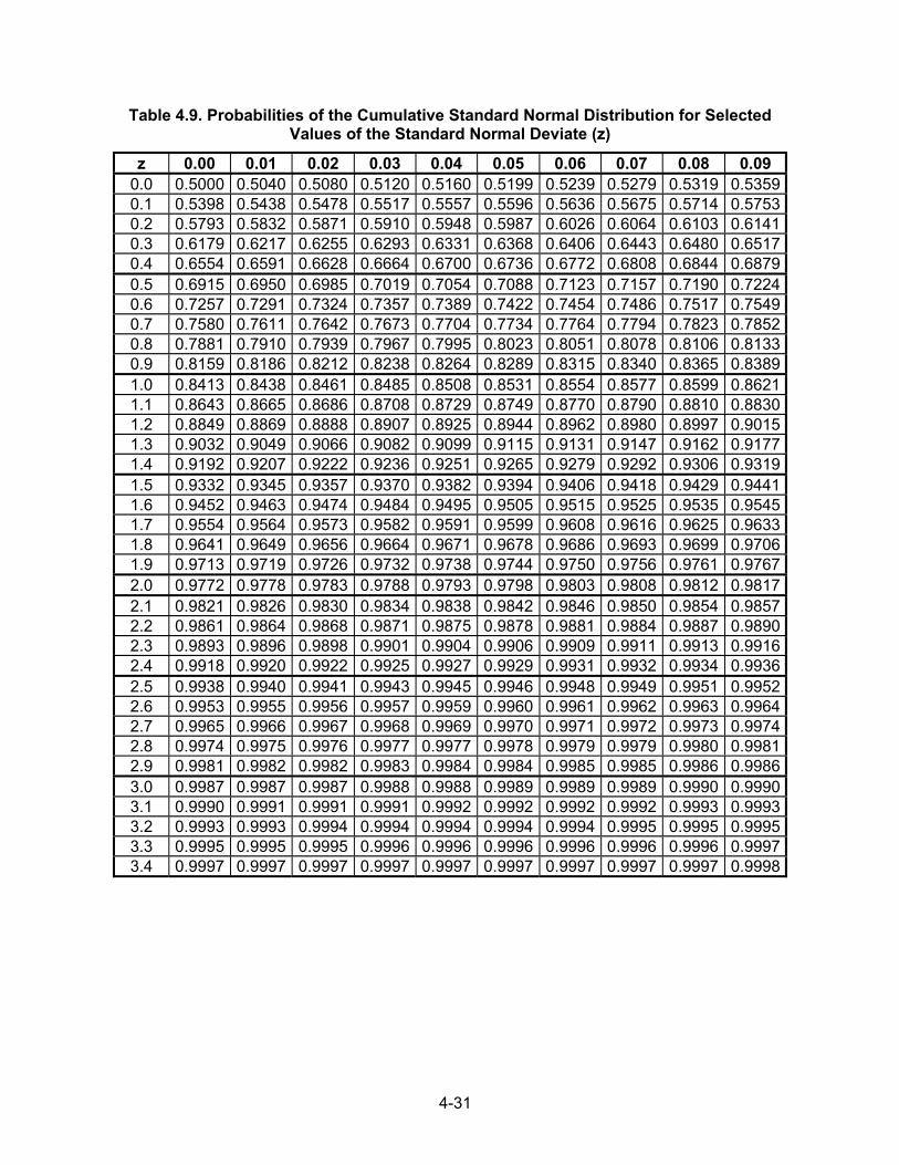
Once the population line has been verified and accepted, the line can be used for estimation. While graphical estimates are acceptable for some work, it is often important to use Equations 4.24 and 4.25 in estimating flood magnitudes or probabilities. To make a probability estimate p for a given magnitude, use the following procedure: 1. Use Equation 4.24 to compute the value of the standard normal deviate. 2. Enter Table 4.9 with the value of z and obtain the exceedence probability. To make estimates of the magnitude for a given exceedence probability, use the following procedure: 1. Enter Table 4.9 with the exceedence probability and obtain the corresponding value of z. 2. Use Equation 4.25 with X, S, and z to compute the magnitude X.

4-30

Table 4.9. Probabilities of the Cumulative Standard Normal Distribution for Selected

Values of the Standard Normal Deviate (z)

z 0.00 0.01 0.02 0.03 0.04 0.05 0.06 0.07 0.08 0.09 -3.4 0.0003 0.0003 0.0003 0.0003 0.0003 0.0003 0.0003 0.0003 0.0003 0.0002-3.3 0.0005 0.0005 0.0005 0.0004 0.0004 0.0004 0.0004 0.0004 0.0004 0.0003-3.2 0.0007 0.0007 0.0006 0.0006 0.0006 0.0006 0.0006 0.0005 0.0005 0.0005-3.1 0.0010 0.0009 0.0009 0.0009 0.0008 0.0008 0.0008 0.0008 0.0007 0.0007-3.0 0.0013 0.0013 0.0013 0.0012 0.0012 0.0011 0.0011 0.0011 0.0010 0.0010-2.9 0.0019 0.0018 0.0018 0.0017 0.0016 0.0016 0.0015 0.0015 0.0014 0.0014-2.8 0.0026 0.0025 0.0024 0.0023 0.0023 0.0022 0.0021 0.0021 0.0020 0.0019-2.7 0.0035 0.0034 0.0033 0.0032 0.0031 0.0030 0.0029 0.0028 0.0027 0.0026-2.6 0.0047 0.0045 0.0044 0.0043 0.0041 0.0040 0.0039 0.0038 0.0037 0.0036-2.5 0.0062 0.0060 0.0059 0.0057 0.0055 0.0054 0.0052 0.0051 0.0049 0.0048-2.4 0.0082 0.0080 0.0078 0.0075 0.0073 0.0071 0.0069 0.0068 0.0066 0.0064-2.3 0.0107 0.0104 0.0102 0.0099 0.0096 0.0094 0.0091 0.0089 0.0087 0.0084-2.2 0.0139 0.0136 0.0132 0.0129 0.0125 0.0122 0.0119 0.0116 0.0113 0.0110-2.1 0.0179 0.0174 0.0170 0.0166 0.0162 0.0158 0.0154 0.0150 0.0146 0.0143-2.0 0.0228 0.0222 0.0217 0.0212 0.0207 0.0202 0.0197 0.0192 0.0188 0.0183-1.9 0.0287 0.0281 0.0274 0.0268 0.0262 0.0256 0.0250 0.0244 0.0239 0.0233-1.8 0.0359 0.0351 0.0344 0.0336 0.0329 0.0322 0.0314 0.0307 0.0301 0.0294-1.7 0.0446 0.0436 0.0427 0.0418 0.0409 0.0401 0.0392 0.0384 0.0375 0.0367-1.6 0.0548 0.0537 0.0526 0.0516 0.0505 0.0495 0.0485 0.0475 0.0465 0.0455-1.5 0.0668 0.0655 0.0643 0.0630 0.0618 0.0606 0.0594 0.0582 0.0571 0.0559-1.4 0.0808 0.0793 0.0778 0.0764 0.0749 0.0735 0.0721 0.0708 0.0694 0.0681-1.3 0.0968 0.0951 0.0934 0.0918 0.0901 0.0885 0.0869 0.0853 0.0838 0.0823-1.2 0.1151 0.1131 0.1112 0.1093 0.1075 0.1056 0.1038 0.1020 0.1003 0.0985-1.1 0.1357 0.1335 0.1314 0.1292 0.1271 0.1251 0.1230 0.1210 0.1190 0.1170-1.0 0.1587 0.1562 0.1539 0.1515 0.1492 0.1469 0.1446 0.1423 0.1401 0.1379-.9 0.1841 0.1814 0.1788 0.1762 0.1736 0.1711 0.1685 0.1660 0.1635 0.1611-.8 0.2119 0.2090 0.2061 0.2033 0.2005 0.1977 0.1949 0.1922 0.1894 0.1867-.7 0.2420 0.2389 0.2358 0.2327 0.2296 0.2266 0.2236 0.2206 0.2177 0.2148-.6 0.2743 0.2709 0.2676 0.2643 0.2611 0.2578 0.2546 0.2514 0.2483 0.2451-.5 0.3085 0.3050 0.3015 0.2981 0.2946 0.2912 0.2877 0.2843 0.2810 0.2776-.4 0.3446 0.3409 0.3372 0.3336 0.3300 0.3264 0.3228 0.3192 0.3156 0.3121-.3 0.3821 0.3783 0.3745 0.3707 0.3669 0.3632 0.3594 0.3557 0.3520 0.3483-.2 0.4207 0.4168 0.4129 0.4090 0.4052 0.4013 0.3974 0.3936 0.3897 0.3859-.1 0.4602 0.4562 0.4522 0.4483 0.4443 0.4404 0.4364 0.4325 0.4286 0.4247-.0 0.5000 0.4960 0.4920 0.4880 0.4840 0.4801 0.4761 0.4721 0.4681 0.4641

4-31

Table 4.9. Probabilities of the Cumulative Standard Normal Distribution for Selected Values of the Standard Normal Deviate (z)

z 0.00 0.01 0.02 0.03 0.04 0.05 0.06 0.07 0.08 0.09 0.0 0.5000 0.5040 0.5080 0.5120 0.5160 0.5199 0.5239 0.5279 0.5319 0.53590.1 0.5398 0.5438 0.5478 0.5517 0.5557 0.5596 0.5636 0.5675 0.5714 0.57530.2 0.5793 0.5832 0.5871 0.5910 0.5948 0.5987 0.6026 0.6064 0.6103 0.61410.3 0.6179 0.6217 0.6255 0.6293 0.6331 0.6368 0.6406 0.6443 0.6480 0.65170.4 0.6554 0.6591 0.6628 0.6664 0.6700 0.6736 0.6772 0.6808 0.6844 0.68790.5 0.6915 0.6950 0.6985 0.7019 0.7054 0.7088 0.7123 0.7157 0.7190 0.72240.6 0.7257 0.7291 0.7324 0.7357 0.7389 0.7422 0.7454 0.7486 0.7517 0.75490.7 0.7580 0.7611 0.7642 0.7673 0.7704 0.7734 0.7764 0.7794 0.7823 0.78520.8 0.7881 0.7910 0.7939 0.7967 0.7995 0.8023 0.8051 0.8078 0.8106 0.81330.9 0.8159 0.8186 0.8212 0.8238 0.8264 0.8289 0.8315 0.8340 0.8365 0.83891.0 0.8413 0.8438 0.8461 0.8485 0.8508 0.8531 0.8554 0.8577 0.8599 0.86211.1 0.8643 0.8665 0.8686 0.8708 0.8729 0.8749 0.8770 0.8790 0.8810 0.88301.2 0.8849 0.8869 0.8888 0.8907 0.8925 0.8944 0.8962 0.8980 0.8997 0.90151.3 0.9032 0.9049 0.9066 0.9082 0.9099 0.9115 0.9131 0.9147 0.9162 0.91771.4 0.9192 0.9207 0.9222 0.9236 0.9251 0.9265 0.9279 0.9292 0.9306 0.93191.5 0.9332 0.9345 0.9357 0.9370 0.9382 0.9394 0.9406 0.9418 0.9429 0.94411.6 0.9452 0.9463 0.9474 0.9484 0.9495 0.9505 0.9515 0.9525 0.9535 0.95451.7 0.9554 0.9564 0.9573 0.9582 0.9591 0.9599 0.9608 0.9616 0.9625 0.96331.8 0.9641 0.9649 0.9656 0.9664 0.9671 0.9678 0.9686 0.9693 0.9699 0.97061.9 0.9713 0.9719 0.9726 0.9732 0.9738 0.9744 0.9750 0.9756 0.9761 0.97672.0 0.9772 0.9778 0.9783 0.9788 0.9793 0.9798 0.9803 0.9808 0.9812 0.98172.1 0.9821 0.9826 0.9830 0.9834 0.9838 0.9842 0.9846 0.9850 0.9854 0.98572.2 0.9861 0.9864 0.9868 0.9871 0.9875 0.9878 0.9881 0.9884 0.9887 0.98902.3 0.9893 0.9896 0.9898 0.9901 0.9904 0.9906 0.9909 0.9911 0.9913 0.99162.4 0.9918 0.9920 0.9922 0.9925 0.9927 0.9929 0.9931 0.9932 0.9934 0.99362.5 0.9938 0.9940 0.9941 0.9943 0.9945 0.9946 0.9948 0.9949 0.9951 0.99522.6 0.9953 0.9955 0.9956 0.9957 0.9959 0.9960 0.9961 0.9962 0.9963 0.99642.7 0.9965 0.9966 0.9967 0.9968 0.9969 0.9970 0.9971 0.9972 0.9973 0.99742.8 0.9974 0.9975 0.9976 0.9977 0.9977 0.9978 0.9979 0.9979 0.9980 0.99812.9 0.9981 0.9982 0.9982 0.9983 0.9984 0.9984 0.9985 0.9985 0.9986 0.99863.0 0.9987 0.9987 0.9987 0.9988 0.9988 0.9989 0.9989 0.9989 0.9990 0.99903.1 0.9990 0.9991 0.9991 0.9991 0.9992 0.9992 0.9992 0.9992 0.9993 0.99933.2 0.9993 0.9993 0.9994 0.9994 0.9994 0.9994 0.9994 0.9995 0.9995 0.99953.3 0.9995 0.9995 0.9995 0.9996 0.9996 0.9996 0.9996 0.9996 0.9996 0.99973.4 0.9997 0.9997 0.9997 0.9997 0.9997 0.9997 0.9997 0.9997 0.9997 0.9998

4-32

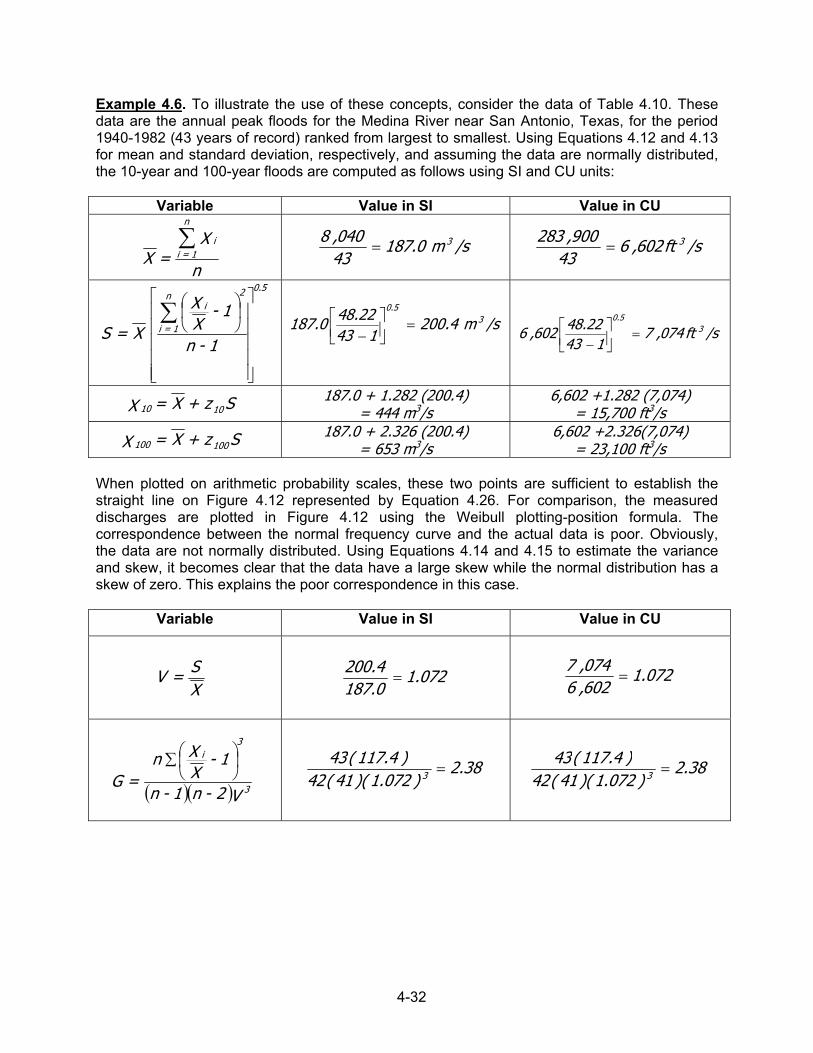
Example 4.6. To illustrate the use of these concepts, consider the data of Table 4.10. These data are the annual peak floods for the Medina River near San Antonio, Texas, for the period 1940-1982 (43 years of record) ranked from largest to smallest. Using Equations 4.12 and 4.13 for mean and standard deviation, respectively, and assuming the data are normally distributed, the 10-year and 100-year floods are computed as follows using SI and CU units:

Variable Value in SI Value in CU

n

X = X

i

n

1 = i∑

/sm 0.187

43040,8 3= /sft602,6

43900,283 3=

∑1 - n

1 - XX

X = S

in

1 = i

2 0.5

/sm 4.200143

22.480.187 35.0

=

−

/sft074,7143

22.48602,6 35.0

=

−

Sz + X = X 1010 187.0 + 1.282 (200.4) = 444 m3/s

6,602 +1.282 (7,074) = 15,700 ft3/s

Sz + X =X 100100 187.0 + 2.326 (200.4) = 653 m3/s

6,602 +2.326(7,074) = 23,100 ft3/s

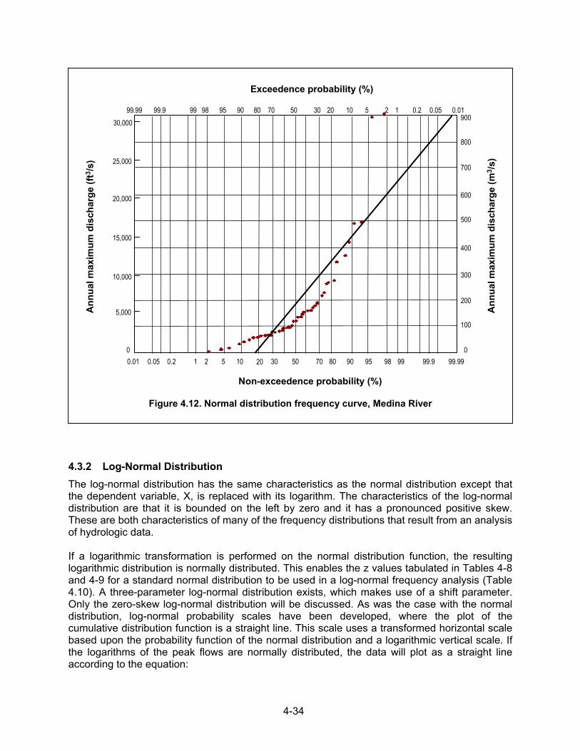
When plotted on arithmetic probability scales, these two points are sufficient to establish the straight line on Figure 4.12 represented by Equation 4.26. For comparison, the measured discharges are plotted in Figure 4.12 using the Weibull plotting-position formula. The correspondence between the normal frequency curve and the actual data is poor. Obviously, the data are not normally distributed. Using Equations 4.14 and 4.15 to estimate the variance and skew, it becomes clear that the data have a large skew while the normal distribution has a skew of zero. This explains the poor correspondence in this case.

Variable Value in SI Value in CU

XS = V 072.1

0.1874.200

= 072.1602,6074,7

=

( )( ) V2-n1-n

1-XXn

= G 3

i3

∑

38.2

)072.1)(41(42)4.117(43

3 = 38.2)072.1)(41(42

)4.117(433 =

4-33

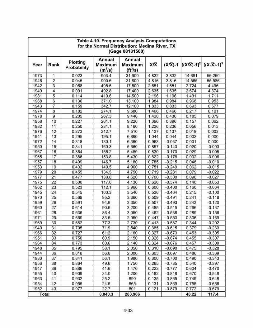
Table 4.10. Frequency Analysis Computations for the Normal Distribution: Medina River, TX

(Gage 08181500)

Year Rank Plotting Probability

Annual Maximum

(m3/s)

Annual Maximum

(ft3/s) X/X (X/X)-1 [(X/X)-1]2 [(X-X)-1]3

1973 1 0.023 903.4 31,900 4.832 3.832 14.681 56.250 1946 2 0.045 900.6 31,800 4.816 3.816 14.565 55.586 1942 3 0.068 495.6 17,500 2.651 1.651 2.724 4.496 1949 4 0.091 492.8 17,400 2.635 1.635 2.674 4.374 1981 5 0.114 410.6 14,500 2.196 1.196 1.431 1.711 1968 6 0.136 371.0 13,100 1.984 0.984 0.968 0.953 1943 7 0.159 342.7 12,100 1.833 0.833 0.693 0.577 1974 8 0.182 274.1 9,680 1.466 0.466 0.217 0.101 1978 9 0.205 267.3 9,440 1.430 0.430 0.185 0.079 1958 10 0.227 261.1 9,220 1.396 0.396 0.157 0.062 1982 11 0.250 231.1 8,160 1.236 0.236 0.056 0.013 1976 12 0.273 212.7 7,510 1.137 0.137 0.019 0.003 1941 13 0.295 195.1 6,890 1.044 0.044 0.002 0.000 1972 14 0.318 180.1 6,360 0.963 -0.037 0.001 0.000 1950 15 0.341 160.3 5,660 0.857 -0.143 0.020 -0.003 1967 16 0.364 155.2 5,480 0.830 -0.170 0.029 -0.005 1965 17 0.386 153.8 5,430 0.822 -0.178 0.032 -0.006 1957 18 0.409 146.7 5,180 0.785 -0.215 0.046 -0.010 1953 19 0.432 140.5 4,960 0.751 -0.249 0.062 -0.015 1979 20 0.455 134.5 4,750 0.719 -0.281 0.079 -0.022 1977 21 0.477 130.8 4,620 0.700 -0.300 0.090 -0.027 1975 22 0.500 117.0 4,130 0.626 -0.374 0.140 -0.053 1962 23 0.523 112.1 3,960 0.600 -0.400 0.160 -0.064 1945 24 0.545 100.3 3,540 0.536 -0.464 0.215 -0.100 1970 25 0.568 95.2 3,360 0.509 -0.491 0.241 -0.118 1959 26 0.591 94.9 3,350 0.507 -0.493 0.243 -0.120 1960 27 0.614 90.6 3,200 0.485 -0.515 0.266 -0.137 1961 28 0.636 86.4 3,050 0.462 -0.538 0.289 -0.156 1971 29 0.659 83.5 2,950 0.447 -0.553 0.306 -0.169 1969 30 0.682 77.3 2,730 0.413 -0.587 0.344 -0.202 1940 31 0.705 71.9 2,540 0.385 -0.615 0.379 -0.233 1966 32 0.727 61.2 2,160 0.327 -0.673 0.453 -0.305 1951 33 0.750 60.9 2,150 0.326 -0.674 0.455 -0.307 1964 34 0.773 60.6 2,140 0.324 -0.676 0.457 -0.309 1948 35 0.795 58.1 2,050 0.310 -0.690 0.475 -0.328 1944 36 0.818 56.6 2,000 0.303 -0.697 0.486 -0.339 1980 37 0.841 56.1 1,980 0.300 -0.700 0.490 -0.343 1956 38 0.864 49.6 1,750 0.265 -0.735 0.540 -0.397 1947 39 0.886 41.6 1,470 0.223 -0.777 0.604 -0.470 1955 40 0.909 34.0 1,200 0.182 -0.818 0.670 -0.548 1963 41 0.932 25.2 890 0.135 -0.865 0.749 -0.648 1954 42 0.955 24.5 865 0.131 -0.869 0.755 -0.656 1952 43 0.977 22.7 801 0.121 -0.879 0.772 -0.679

Total 8,040.3 283,906 48.22 117.4

4-34

4.3.2 Log-Normal Distribution The log-normal distribution has the same characteristics as the normal distribution except that the dependent variable, X, is replaced with its logarithm. The characteristics of the log-normal distribution are that it is bounded on the left by zero and it has a pronounced positive skew. These are both characteristics of many of the frequency distributions that result from an analysis of hydrologic data. If a logarithmic transformation is performed on the normal distribution function, the resulting logarithmic distribution is normally distributed. This enables the z values tabulated in Tables 4-8 and 4-9 for a standard normal distribution to be used in a log-normal frequency analysis (Table 4.10). A three-parameter log-normal distribution exists, which makes use of a shift parameter. Only the zero-skew log-normal distribution will be discussed. As was the case with the normal distribution, log-normal probability scales have been developed, where the plot of the cumulative distribution function is a straight line. This scale uses a transformed horizontal scale based upon the probability function of the normal distribution and a logarithmic vertical scale. If the logarithms of the peak flows are normally distributed, the data will plot as a straight line according to the equation:

900

600

400

200

99.99 99.9 99 98 95 90 80 70 50 30 0.05 0.010.215 21020

99.9999.999989590807050300.050.01 0.2 1 52 10 20

Exceedence probability (%)

100

500

300

0

800

700

Ann

ual m

axim

um d

isch

arge

(m3 /s

)

Ann

ual m

axim

um d

isch

arge

(ft3

/s)

10,000

0

15,000

20,000

25,000

30,000

5,000

Non-exceedence probability (%)

Figure 4.12. Normal distribution frequency curve, Medina River

4-35

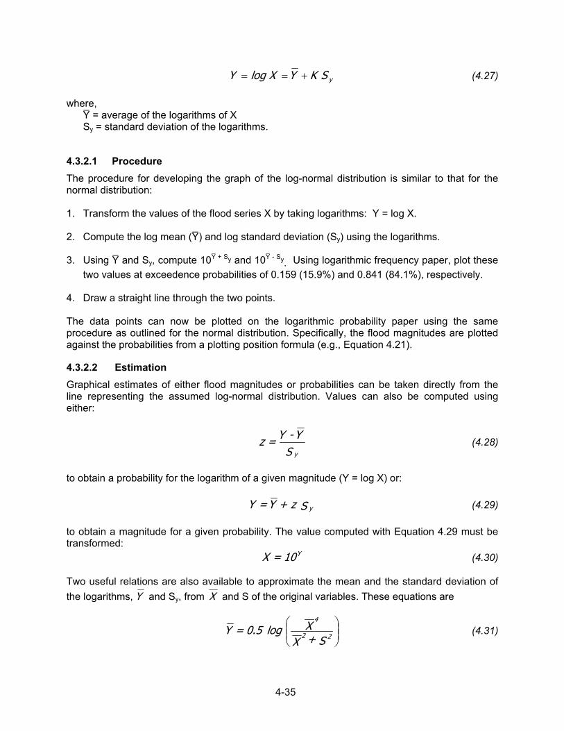
ySKYXlogY +== (4.27) where, Y = average of the logarithms of X Sy = standard deviation of the logarithms.

4.3.2.1 Procedure The procedure for developing the graph of the log-normal distribution is similar to that for the normal distribution: 1. Transform the values of the flood series X by taking logarithms: Y = log X. 2. Compute the log mean (Y) and log standard deviation (Sy) using the logarithms. 3. Using Y and Sy, compute 10Y + Sy and 10Y - Sy. Using logarithmic frequency paper, plot these

two values at exceedence probabilities of 0.159 (15.9%) and 0.841 (84.1%), respectively. 4. Draw a straight line through the two points. The data points can now be plotted on the logarithmic probability paper using the same procedure as outlined for the normal distribution. Specifically, the flood magnitudes are plotted against the probabilities from a plotting position formula (e.g., Equation 4.21).

4.3.2.2 Estimation Graphical estimates of either flood magnitudes or probabilities can be taken directly from the line representing the assumed log-normal distribution. Values can also be computed using either:

S

Y - Y = zy

(4.28)

to obtain a probability for the logarithm of a given magnitude (Y = log X) or: S z + Y = Y y (4.29) to obtain a magnitude for a given probability. The value computed with Equation 4.29 must be transformed: Y10 = X (4.30) Two useful relations are also available to approximate the mean and the standard deviation of the logarithms, Y and Sy, from X and S of the original variables. These equations are

S + XX log 0.5 = Y

22

4

(4.31)

4-36

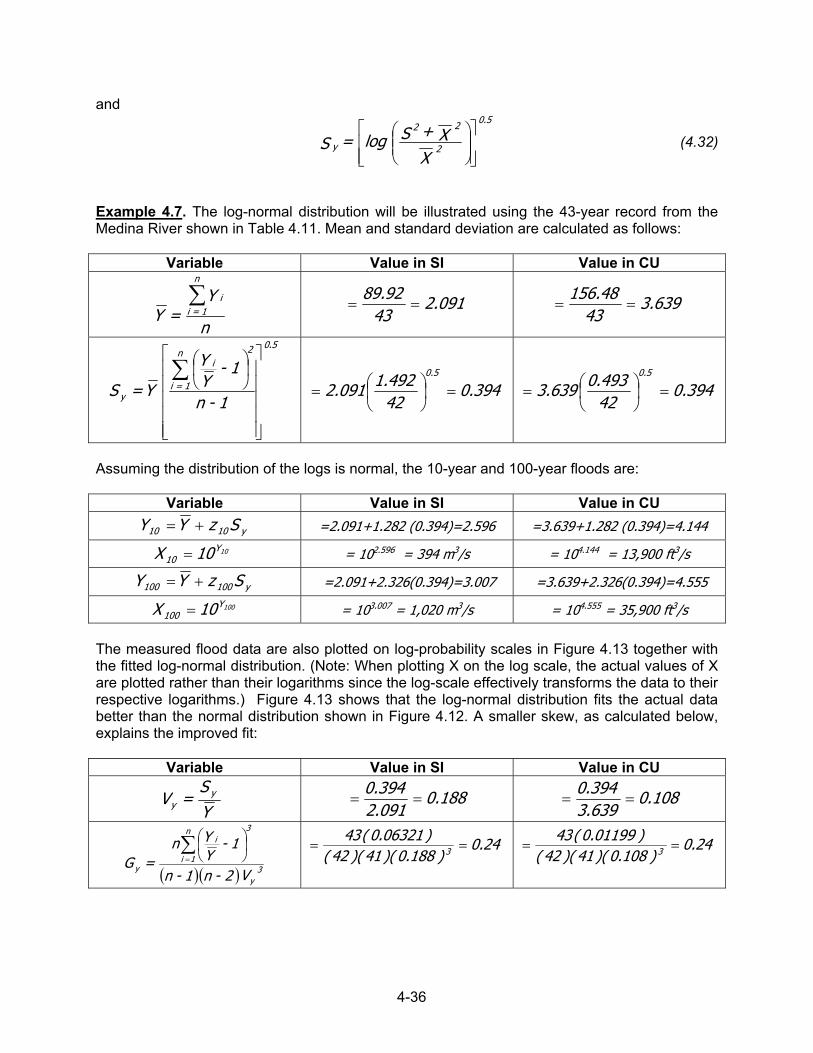
and

XX + S log = S 2

220.5

y (4.32)

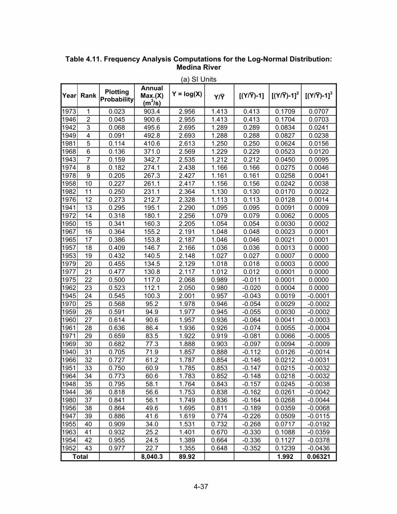
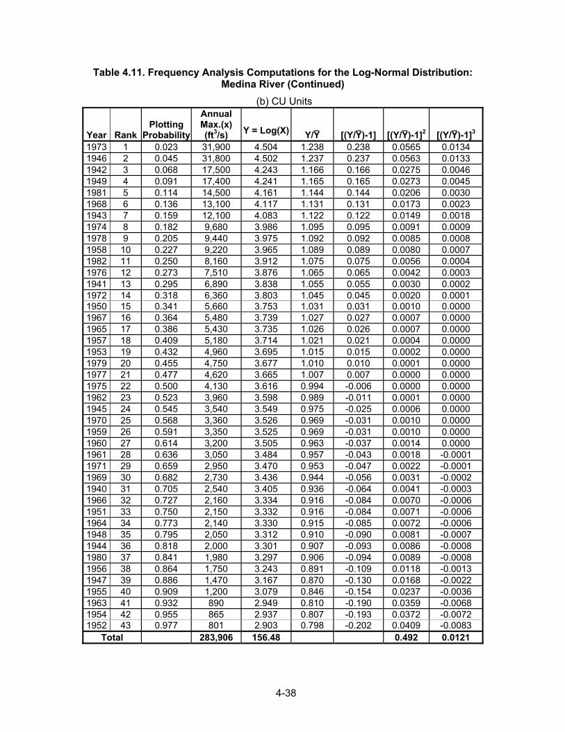
Example 4.7. The log-normal distribution will be illustrated using the 43-year record from the Medina River shown in Table 4.11. Mean and standard deviation are calculated as follows:

Variable Value in SI Value in CU

n

Y = Y

i

n

1 = i∑

091.2

4392.89

== 639.343

48.156==

∑1 - n

1 - YY

Y = S

in

1 = i

2 0.5

y 394.042492.1091.2

5.0

=

= 394.0

42493.0639.3

5.0

=

=

Assuming the distribution of the logs is normal, the 10-year and 100-year floods are:

Variable Value in SI Value in CU

y1010 SzYY += =2.091+1.282 (0.394)=2.596 =3.639+1.282 (0.394)=4.144

10Y10 10X = = 102.596 = 394 m3/s = 104.144 = 13,900 ft3/s

y100100 SzYY += =2.091+2.326(0.394)=3.007 =3.639+2.326(0.394)=4.555

100Y100 10X = = 103.007 = 1,020 m3/s = 104.555 = 35,900 ft3/s

The measured flood data are also plotted on log-probability scales in Figure 4.13 together with the fitted log-normal distribution. (Note: When plotting X on the log scale, the actual values of X are plotted rather than their logarithms since the log-scale effectively transforms the data to their respective logarithms.) Figure 4.13 shows that the log-normal distribution fits the actual data better than the normal distribution shown in Figure 4.12. A smaller skew, as calculated below, explains the improved fit:

Variable Value in SI Value in CU

YS

= V yy 188.0

091.2394.0 == 108.0

639.3394.0 ==

( )( ) y3

n

1i

i3

y V2-n1-n

1-YYn

= G∑

=

24.0

)188.0)(41)(42()06321.0(43

3 ==

24.0)108.0)(41)(42(

)01199.0(433 ==

4-37

Table 4.11. Frequency Analysis Computations for the Log-Normal Distribution:

Medina River (a) SI Units

Year Rank Plotting Probability

Annual Max.(X) (m3/s)

Y = log(X) Y/Y [(Y/Y)-1] [(Y/Y)-1]2 [(Y/Y)-1]3

1973 1 0.023 903.4 2.956 1.413 0.413 0.1709 0.0707 1946 2 0.045 900.6 2.955 1.413 0.413 0.1704 0.0703 1942 3 0.068 495.6 2.695 1.289 0.289 0.0834 0.0241 1949 4 0.091 492.8 2.693 1.288 0.288 0.0827 0.0238 1981 5 0.114 410.6 2.613 1.250 0.250 0.0624 0.0156 1968 6 0.136 371.0 2.569 1.229 0.229 0.0523 0.0120 1943 7 0.159 342.7 2.535 1.212 0.212 0.0450 0.0095 1974 8 0.182 274.1 2.438 1.166 0.166 0.0275 0.0046 1978 9 0.205 267.3 2.427 1.161 0.161 0.0258 0.0041 1958 10 0.227 261.1 2.417 1.156 0.156 0.0242 0.0038 1982 11 0.250 231.1 2.364 1.130 0.130 0.0170 0.0022 1976 12 0.273 212.7 2.328 1.113 0.113 0.0128 0.0014 1941 13 0.295 195.1 2.290 1.095 0.095 0.0091 0.0009 1972 14 0.318 180.1 2.256 1.079 0.079 0.0062 0.0005 1950 15 0.341 160.3 2.205 1.054 0.054 0.0030 0.0002 1967 16 0.364 155.2 2.191 1.048 0.048 0.0023 0.0001 1965 17 0.386 153.8 2.187 1.046 0.046 0.0021 0.0001 1957 18 0.409 146.7 2.166 1.036 0.036 0.0013 0.0000 1953 19 0.432 140.5 2.148 1.027 0.027 0.0007 0.0000 1979 20 0.455 134.5 2.129 1.018 0.018 0.0003 0.0000 1977 21 0.477 130.8 2.117 1.012 0.012 0.0001 0.0000 1975 22 0.500 117.0 2.068 0.989 -0.011 0.0001 0.0000 1962 23 0.523 112.1 2.050 0.980 -0.020 0.0004 0.0000 1945 24 0.545 100.3 2.001 0.957 -0.043 0.0019 -0.0001 1970 25 0.568 95.2 1.978 0.946 -0.054 0.0029 -0.0002 1959 26 0.591 94.9 1.977 0.945 -0.055 0.0030 -0.0002 1960 27 0.614 90.6 1.957 0.936 -0.064 0.0041 -0.0003 1961 28 0.636 86.4 1.936 0.926 -0.074 0.0055 -0.0004 1971 29 0.659 83.5 1.922 0.919 -0.081 0.0066 -0.0005 1969 30 0.682 77.3 1.888 0.903 -0.097 0.0094 -0.0009 1940 31 0.705 71.9 1.857 0.888 -0.112 0.0126 -0.0014 1966 32 0.727 61.2 1.787 0.854 -0.146 0.0212 -0.0031 1951 33 0.750 60.9 1.785 0.853 -0.147 0.0215 -0.0032 1964 34 0.773 60.6 1.783 0.852 -0.148 0.0218 -0.0032 1948 35 0.795 58.1 1.764 0.843 -0.157 0.0245 -0.0038 1944 36 0.818 56.6 1.753 0.838 -0.162 0.0261 -0.0042 1980 37 0.841 56.1 1.749 0.836 -0.164 0.0268 -0.0044 1956 38 0.864 49.6 1.695 0.811 -0.189 0.0359 -0.0068 1947 39 0.886 41.6 1.619 0.774 -0.226 0.0509 -0.0115 1955 40 0.909 34.0 1.531 0.732 -0.268 0.0717 -0.0192 1963 41 0.932 25.2 1.401 0.670 -0.330 0.1088 -0.0359 1954 42 0.955 24.5 1.389 0.664 -0.336 0.1127 -0.0378 1952 43 0.977 22.7 1.355 0.648 -0.352 0.1239 -0.0436

Total 8,040.3 89.92 1.992 0.06321

4-38

Table 4.11. Frequency Analysis Computations for the Log-Normal Distribution: Medina River (Continued)

(b) CU Units

Year Rank Plotting

Probability

Annual Max.(x) (ft3/s) Y = Log(X) Y/Y [(Y/Y)-1] [(Y/Y)-1]2 [(Y/Y)-1]3

1973 1 0.023 31,900 4.504 1.238 0.238 0.0565 0.0134 1946 2 0.045 31,800 4.502 1.237 0.237 0.0563 0.0133 1942 3 0.068 17,500 4.243 1.166 0.166 0.0275 0.0046 1949 4 0.091 17,400 4.241 1.165 0.165 0.0273 0.0045 1981 5 0.114 14,500 4.161 1.144 0.144 0.0206 0.0030 1968 6 0.136 13,100 4.117 1.131 0.131 0.0173 0.0023 1943 7 0.159 12,100 4.083 1.122 0.122 0.0149 0.0018 1974 8 0.182 9,680 3.986 1.095 0.095 0.0091 0.0009 1978 9 0.205 9,440 3.975 1.092 0.092 0.0085 0.0008 1958 10 0.227 9,220 3.965 1.089 0.089 0.0080 0.0007 1982 11 0.250 8,160 3.912 1.075 0.075 0.0056 0.0004 1976 12 0.273 7,510 3.876 1.065 0.065 0.0042 0.0003 1941 13 0.295 6,890 3.838 1.055 0.055 0.0030 0.0002 1972 14 0.318 6,360 3.803 1.045 0.045 0.0020 0.0001 1950 15 0.341 5,660 3.753 1.031 0.031 0.0010 0.0000 1967 16 0.364 5,480 3.739 1.027 0.027 0.0007 0.0000 1965 17 0.386 5,430 3.735 1.026 0.026 0.0007 0.0000 1957 18 0.409 5,180 3.714 1.021 0.021 0.0004 0.0000 1953 19 0.432 4,960 3.695 1.015 0.015 0.0002 0.0000 1979 20 0.455 4,750 3.677 1.010 0.010 0.0001 0.0000 1977 21 0.477 4,620 3.665 1.007 0.007 0.0000 0.0000 1975 22 0.500 4,130 3.616 0.994 -0.006 0.0000 0.0000 1962 23 0.523 3,960 3.598 0.989 -0.011 0.0001 0.0000 1945 24 0.545 3,540 3.549 0.975 -0.025 0.0006 0.0000 1970 25 0.568 3,360 3.526 0.969 -0.031 0.0010 0.0000 1959 26 0.591 3,350 3.525 0.969 -0.031 0.0010 0.0000 1960 27 0.614 3,200 3.505 0.963 -0.037 0.0014 0.0000 1961 28 0.636 3,050 3.484 0.957 -0.043 0.0018 -0.0001 1971 29 0.659 2,950 3.470 0.953 -0.047 0.0022 -0.0001 1969 30 0.682 2,730 3.436 0.944 -0.056 0.0031 -0.0002 1940 31 0.705 2,540 3.405 0.936 -0.064 0.0041 -0.0003 1966 32 0.727 2,160 3.334 0.916 -0.084 0.0070 -0.0006 1951 33 0.750 2,150 3.332 0.916 -0.084 0.0071 -0.0006 1964 34 0.773 2,140 3.330 0.915 -0.085 0.0072 -0.0006 1948 35 0.795 2,050 3.312 0.910 -0.090 0.0081 -0.0007 1944 36 0.818 2,000 3.301 0.907 -0.093 0.0086 -0.0008 1980 37 0.841 1,980 3.297 0.906 -0.094 0.0089 -0.0008 1956 38 0.864 1,750 3.243 0.891 -0.109 0.0118 -0.0013 1947 39 0.886 1,470 3.167 0.870 -0.130 0.0168 -0.0022 1955 40 0.909 1,200 3.079 0.846 -0.154 0.0237 -0.0036 1963 41 0.932 890 2.949 0.810 -0.190 0.0359 -0.0068 1954 42 0.955 865 2.937 0.807 -0.193 0.0372 -0.0072 1952 43 0.977 801 2.903 0.798 -0.202 0.0409 -0.0083

Total 283,906 156.48 0.492 0.0121

4-39

4.3.3 Gumbel Extreme Value Distribution The Gumbel extreme value distribution, sometimes called the double-exponential distribution of extreme values, can also be used to describe the distribution of hydrologic variables, especially peak discharges. It is based upon the assumption that the cumulative frequency distribution of the largest values of samples drawn from a large population can be described by the following equation:

e = F(X) e )- (X- βα (4.33)

99.99 99.9 99 98 95 90 80 70 50 30 0.05 0.010.215 21020

99.9999.999989590807050300.050.01 0.2 1 52 10 20

500

10

Exceedence probability (%)D

isch

arge

(ft3

/s)

95% Confidence interval, one sided

Non-exceedence probability (%)

Dis

char

ge (m

3 /s)

1,000

5,000

10,000

20,000

30,00010,000800

600

400

200

10080

60

40

20

10

Figure 4.13. Log-normal distribution frequency curve (solid line) and one-sided upper confidence interval (dashed line)

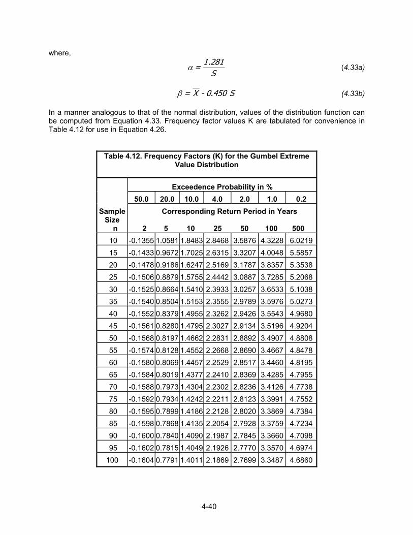
4-40

where,

S281.1 = α (4.33a)

S 0.450 - X = β (4.33b) In a manner analogous to that of the normal distribution, values of the distribution function can be computed from Equation 4.33. Frequency factor values K are tabulated for convenience in Table 4.12 for use in Equation 4.26.

Table 4.12. Frequency Factors (K) for the Gumbel Extreme

Value Distribution

Exceedence Probability in %

50.0

20.0

10.0

4.0

2.0

1.0

0.2

Sample Size n

2

Corresponding Return Period in Years 5 10 25 50 100 500

10 -0.1355

1.0581

1.8483

2.8468

3.5876

4.3228

6.0219

15 -0.1433

0.9672

1.7025

2.6315

3.3207

4.0048

5.5857

20 -0.1478

0.9186

1.6247

2.5169

3.1787

3.8357

5.3538

25 -0.1506

0.8879

1.5755

2.4442

3.0887

3.7285

5.2068

30 -0.1525

0.8664

1.5410

2.3933

3.0257

3.6533

5.1038

35 -0.1540

0.8504

1.5153

2.3555

2.9789

3.5976

5.0273

40 -0.1552

0.8379

1.4955

2.3262

2.9426

3.5543

4.9680

45 -0.1561

0.8280

1.4795

2.3027

2.9134

3.5196

4.9204

50 -0.1568

0.8197

1.4662

2.2831

2.8892

3.4907

4.8808

55 -0.1574

0.8128

1.4552

2.2668

2.8690

3.4667

4.8478

60 -0.1580

0.8069

1.4457

2.2529

2.8517

3.4460

4.8195

65 -0.1584

0.8019

1.4377

2.2410

2.8369

3.4285

4.7955

70 -0.1588

0.7973

1.4304

2.2302

2.8236

3.4126

4.7738

75 -0.1592

0.7934

1.4242

2.2211

2.8123

3.3991

4.7552

80 -0.1595

0.7899

1.4186

2.2128

2.8020

3.3869

4.7384

85 -0.1598

0.7868

1.4135

2.2054

2.7928

3.3759

4.7234

90 -0.1600

0.7840

1.4090

2.1987

2.7845

3.3660

4.7098

95 -0.1602

0.7815

1.4049

2.1926

2.7770

3.3570

4.6974

100 -0.1604

0.7791

1.4011

2.1869

2.7699

3.3487

4.6860

4-41

Characteristics of the Gumbel extreme-value distribution are that the mean flow, X, occurs at the return period of Tr = 2.33 years and that it has a positive skew (i.e., it is skewed toward the high flows or extreme values). As was the case with the two previous distributions, special probability scales have been developed so that sample data, if they are distributed according to Equation 4.33, will plot as a straight line. Most USGS offices have prepared forms with these axis on which the horizontal scale has been transformed by the double-logarithmic transform of Equation 4.33. Example 4.8. Peak flow data for the Medina River can be fit with a Gumbel distribution using Equation 4.26 and values of K from Table 4.12. The mean and standard deviation were calculated earlier as 187.0 m3 /s (6,602 ft3 /s) and 200.4 m3 /s (7,074 ft3 /s), respectively. The 10-year flood computed from the Gumbel distribution is:

Variable Value in SI Value in CU

KS + X X 10 = 187.0 + 1.486 (200.4) = 485 m3 /s 6,602 + 1.486 (7,074) = 17,100 ft3 /s

and the 100-year flood is:

Variable Value in SI Value in CU

KS + X =X 100 187.0 + 3.534 (200.4) = 895 m3 /s 6,602 + 3.534 (7,074) = 31,600 ft3 /s

Plotted on the Gumbel graph in Figure 4.14 are the actual flood data and the computed frequency curve. Although the Gumbel distribution is skewed positively, it does not account directly for the computed skew of the data, but does predict the high flows reasonably well. However, the entire curve fit is not much better than that obtained with the normal distribution, indicating this peak flow series is not distributed according to the double-exponential distribution of Equation 4.33.

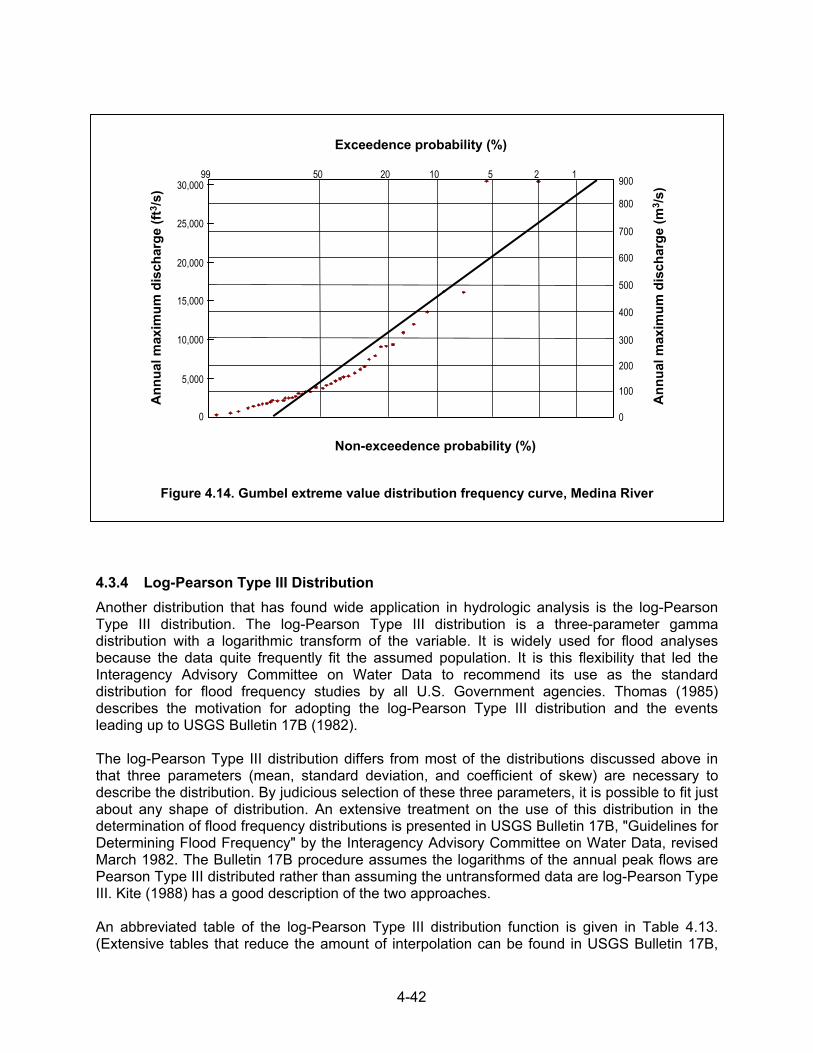
4-42

4.3.4 Log-Pearson Type III Distribution Another distribution that has found wide application in hydrologic analysis is the log-Pearson Type III distribution. The log-Pearson Type III distribution is a three-parameter gamma distribution with a logarithmic transform of the variable. It is widely used for flood analyses because the data quite frequently fit the assumed population. It is this flexibility that led the Interagency Advisory Committee on Water Data to recommend its use as the standard distribution for flood frequency studies by all U.S. Government agencies. Thomas (1985) describes the motivation for adopting the log-Pearson Type III distribution and the events leading up to USGS Bulletin 17B (1982). The log-Pearson Type III distribution differs from most of the distributions discussed above in that three parameters (mean, standard deviation, and coefficient of skew) are necessary to describe the distribution. By judicious selection of these three parameters, it is possible to fit just about any shape of distribution. An extensive treatment on the use of this distribution in the determination of flood frequency distributions is presented in USGS Bulletin 17B, "Guidelines for Determining Flood Frequency" by the Interagency Advisory Committee on Water Data, revised March 1982. The Bulletin 17B procedure assumes the logarithms of the annual peak flows are Pearson Type III distributed rather than assuming the untransformed data are log-Pearson Type III. Kite (1988) has a good description of the two approaches. An abbreviated table of the log-Pearson Type III distribution function is given in Table 4.13. (Extensive tables that reduce the amount of interpolation can be found in USGS Bulletin 17B,

900

600

400

200

Exceedence probability (%)

100

500

300

0

800

700

99 50 15 21020A

nnua

l max

imum

dis

char

ge (f

t3/s

)

Ann

ual m

axim

um d

isch

arge

(m3 /s

)30,000

25,000

20,000

15,000

10,000

5,000

0

Non-exceedence probability (%)

Figure 4.14. Gumbel extreme value distribution frequency curve, Medina River

4-43

1982.) Using the mean, standard deviation, and skew coefficient for any set of log-transformed annual peak flow data, in conjunction with Table 4.13, the flood with any exceedence frequency can be computed from the equation:

yKS+ Y = Xlog = Y (4.34) where Y is the predicted value of log X, Y and Sy are as previously defined, and K is a function of the exceedence probability and the coefficient of skew. Again, it would be possible to develop special probability scales, so that the log-Pearson Type III distribution would plot as a straight line. However, the log-Pearson Type III distribution can assume a variety of shapes so that a separate probability scale would be required for each different shape. Since this is impractical, log-Pearson Type III distributions are usually plotted on log-normal probability scales even though the plotted frequency distribution may not be a straight line. It is a straight line only when the skew of the logarithms is zero.

4.3.4.1 Procedure The procedure for fitting the log-Pearson Type III distribution is similar to that for the normal and log-normal. The specific steps for making a basic log-Pearson Type III analysis without any of the optional adjustments are as follows: 1. Make a logarithmic transform of all flows in the series (Yi = log Xi). 2. Compute the mean (Y), standard deviation (Sy), and standardized skew (G) of the

logarithms using Equations 4.12, 4.13, and 4.15, respectively. Round the skew to the nearest tenth (e.g., 0.32 is rounded to 0.3).

3. Since the log-Pearson Type III curve with a nonzero skew does not plot as a straight line, it

is necessary to use more than two points to draw the curve. The curvature of the line will increase as the absolute value of the skew increases, so more points will be needed for larger skew magnitudes.

4. Compute the logarithmic valueY for each exceedence frequency using Equation 4.34.

5. Transform the computed values of step 4 to discharges using equation 4.35:

Y10= X (4.35) in which X

) is the computed discharge for the assumed log-Pearson Type III population.

6. Plot the points of step 5 on logarithmic probability paper and draw a smooth curve through

the points. The sample data can be plotted on the paper using a plotting position formula to obtain the exceedence probability. The computed curve can then be verified, and, if acceptable, it can be used to make estimates of either a flood probability or flood magnitude.

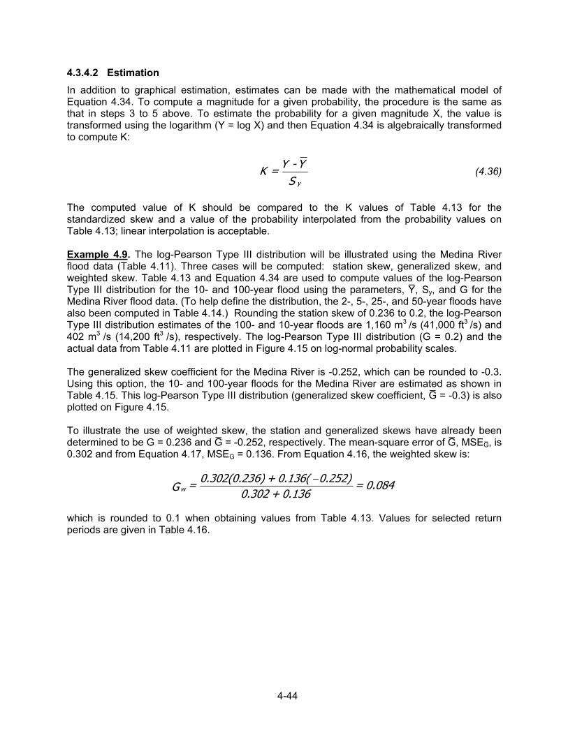
4-44

4.3.4.2 Estimation In addition to graphical estimation, estimates can be made with the mathematical model of Equation 4.34. To compute a magnitude for a given probability, the procedure is the same as that in steps 3 to 5 above. To estimate the probability for a given magnitude X, the value is transformed using the logarithm (Y = log X) and then Equation 4.34 is algebraically transformed to compute K:

S

Y - Y = Ky

(4.36)

The computed value of K should be compared to the K values of Table 4.13 for the standardized skew and a value of the probability interpolated from the probability values on Table 4.13; linear interpolation is acceptable. Example 4.9. The log-Pearson Type III distribution will be illustrated using the Medina River flood data (Table 4.11). Three cases will be computed: station skew, generalized skew, and weighted skew. Table 4.13 and Equation 4.34 are used to compute values of the log-Pearson Type III distribution for the 10- and 100-year flood using the parameters, Y, Sy, and G for the Medina River flood data. (To help define the distribution, the 2-, 5-, 25-, and 50-year floods have also been computed in Table 4.14.) Rounding the station skew of 0.236 to 0.2, the log-Pearson Type III distribution estimates of the 100- and 10-year floods are 1,160 m3 /s (41,000 ft3 /s) and 402 m3 /s (14,200 ft3 /s), respectively. The log-Pearson Type III distribution (G = 0.2) and the actual data from Table 4.11 are plotted in Figure 4.15 on log-normal probability scales. The generalized skew coefficient for the Medina River is -0.252, which can be rounded to -0.3. Using this option, the 10- and 100-year floods for the Medina River are estimated as shown in Table 4.15. This log-Pearson Type III distribution (generalized skew coefficient, G = -0.3) is also plotted on Figure 4.15. To illustrate the use of weighted skew, the station and generalized skews have already been determined to be G = 0.236 and G = -0.252, respectively. The mean-square error of G, MSEG, is 0.302 and from Equation 4.17, MSEG = 0.136. From Equation 4.16, the weighted skew is:

0.084 = 0.136 + 0.302

0.252)0.136(+6)0.302(0.23 = G w−

which is rounded to 0.1 when obtaining values from Table 4.13. Values for selected return periods are given in Table 4.16.

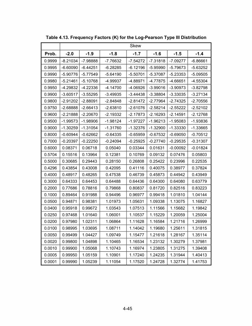
4-45

Table 4.13. Frequency Factors (K) for the Log-Pearson Type III Distribution

Skew

Prob. -2.0 -1.9 -1.8 -1.7 -1.6 -1.5 -1.4 0.9999 -8.21034 -7.98888 -7.76632 -7.54272 -7.31818 -7.09277 -6.86661 0.9995 -6.60090 -6.44251 -6.28285 -6.12196 -5.95990 -5.79673 -5.63252 0.9990 -5.90776 -5.77549 -5.64190 -5.50701 -5.37087 -5.23353 -5.09505 0.9980 -5.21461 -5.10768 -4.99937 -4.88971 -4.77875 -4.66651 -4.55304 0.9950 -4.29832 -4.22336 -4.14700 -4.06926 -3.99016 -3.90973 -3.82798 0.9900 -3.60517 -3.55295 -3.49935 -3.44438 -3.38804 -3.33035 -3.27134 0.9800 -2.91202 -2.88091 -2.84848 -2.81472 -2.77964 -2.74325 -2.70556 0.9750 -2.68888 -2.66413 -2.63810 -2.61076 -2.58214 -2.55222 -2.52102 0.9600 -2.21888 -2.20670 -2.19332 -2.17873 -2.16293 -2.14591 -2.12768 0.9500 -1.99573 -1.98906 -1.98124 -1.97227 -1.96213 -1.95083 -1.93836 0.9000 -1.30259 -1.31054 -1.31760 -1.32376 -1.32900 -1.33330 -1.33665 0.8000 -0.60944 -0.62662 -0.64335 -0.65959 -0.67532 -0.69050 -0.70512 0.7000 -0.20397 -0.22250 -0.24094 -0.25925 -0.27740 -0.29535 -0.31307 0.6000 0.08371 0.06718 0.05040 0.03344 0.01631 -0.00092 -0.01824 0.5704 0.15516 0.13964 0.12381 0.10769 0.09132 0.07476 0.05803 0.5000 0.30685 0.29443 0.28150 0.26808 0.25422 0.23996 0.22535 0.4296 0.43854 0.43008 0.42095 0.41116 0.40075 0.38977 0.37824 0.4000 0.48917 0.48265 0.47538 0.46739 0.45873 0.44942 0.43949 0.3000 0.64333 0.64453 0.64488 0.64436 0.64300 0.64080 0.63779 0.2000 0.77686 0.78816 0.79868 0.80837 0.81720 0.82516 0.83223 0.1000 0.89464 0.91988 0.94496 0.96977 0.99418 1.01810 1.04144 0.0500 0.94871 0.98381 1.01973 1.05631 1.09338 1.13075 1.16827 0.0400 0.95918 0.99672 1.03543 1.07513 1.11566 1.15682 1.19842 0.0250 0.97468 1.01640 1.06001 1.10537 1.15229 1.20059 1.25004 0.0200 0.97980 1.02311 1.06864 1.11628 1.16584 1.21716 1.26999 0.0100 0.98995 1.03695 1.08711 1.14042 1.19680 1.25611 1.31815 0.0050 0.99499 1.04427 1.09749 1.15477 1.21618 1.28167 1.35114 0.0020 0.99800 1.04898 1.10465 1.16534 1.23132 1.30279 1.37981 0.0010 0.99900 1.05068 1.10743 1.16974 1.23805 1.31275 1.39408 0.0005 0.99950 1.05159 1.10901 1.17240 1.24235 1.31944 1.40413 0.0001 0.99990 1.05239 1.11054 1.17520 1.24728 1.32774 1.41753

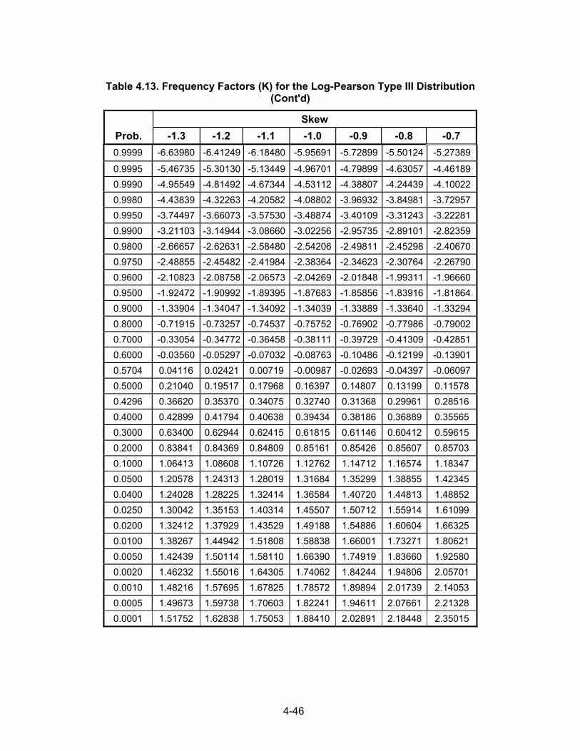
4-46

Table 4.13. Frequency Factors (K) for the Log-Pearson Type III Distribution

(Cont'd)

Skew Prob. -1.3 -1.2 -1.1 -1.0 -0.9 -0.8 -0.7 0.9999 -6.63980 -6.41249 -6.18480 -5.95691 -5.72899 -5.50124 -5.27389

0.9995 -5.46735 -5.30130 -5.13449 -4.96701 -4.79899 -4.63057 -4.46189 0.9990 -4.95549 -4.81492 -4.67344 -4.53112 -4.38807 -4.24439 -4.10022 0.9980 -4.43839 -4.32263 -4.20582 -4.08802 -3.96932 -3.84981 -3.72957 0.9950 -3.74497 -3.66073 -3.57530 -3.48874 -3.40109 -3.31243 -3.22281 0.9900 -3.21103 -3.14944 -3.08660 -3.02256 -2.95735 -2.89101 -2.82359 0.9800 -2.66657 -2.62631 -2.58480 -2.54206 -2.49811 -2.45298 -2.40670 0.9750 -2.48855 -2.45482 -2.41984 -2.38364 -2.34623 -2.30764 -2.26790 0.9600 -2.10823 -2.08758 -2.06573 -2.04269 -2.01848 -1.99311 -1.96660 0.9500 -1.92472 -1.90992 -1.89395 -1.87683 -1.85856 -1.83916 -1.81864 0.9000 -1.33904 -1.34047 -1.34092 -1.34039 -1.33889 -1.33640 -1.33294 0.8000 -0.71915 -0.73257 -0.74537 -0.75752 -0.76902 -0.77986 -0.79002 0.7000 -0.33054 -0.34772 -0.36458 -0.38111 -0.39729 -0.41309 -0.42851 0.6000 -0.03560 -0.05297 -0.07032 -0.08763 -0.10486 -0.12199 -0.13901 0.5704 0.04116 0.02421 0.00719 -0.00987 -0.02693 -0.04397 -0.06097 0.5000 0.21040 0.19517 0.17968 0.16397 0.14807 0.13199 0.11578 0.4296 0.36620 0.35370 0.34075 0.32740 0.31368 0.29961 0.28516 0.4000 0.42899 0.41794 0.40638 0.39434 0.38186 0.36889 0.35565 0.3000 0.63400 0.62944 0.62415 0.61815 0.61146 0.60412 0.59615 0.2000 0.83841 0.84369 0.84809 0.85161 0.85426 0.85607 0.85703 0.1000 1.06413 1.08608 1.10726 1.12762 1.14712 1.16574 1.18347 0.0500 1.20578 1.24313 1.28019 1.31684 1.35299 1.38855 1.42345 0.0400 1.24028 1.28225 1.32414 1.36584 1.40720 1.44813 1.48852 0.0250 1.30042 1.35153 1.40314 1.45507 1.50712 1.55914 1.61099 0.0200 1.32412 1.37929 1.43529 1.49188 1.54886 1.60604 1.66325 0.0100 1.38267 1.44942 1.51808 1.58838 1.66001 1.73271 1.80621 0.0050 1.42439 1.50114 1.58110 1.66390 1.74919 1.83660 1.92580 0.0020 1.46232 1.55016 1.64305 1.74062 1.84244 1.94806 2.05701 0.0010 1.48216 1.57695 1.67825 1.78572 1.89894 2.01739 2.14053 0.0005 1.49673 1.59738 1.70603 1.82241 1.94611 2.07661 2.21328 0.0001 1.51752 1.62838 1.75053 1.88410 2.02891 2.18448 2.35015

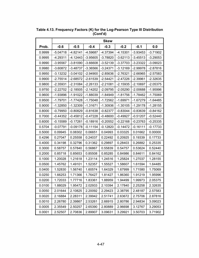
4-47

Table 4.13. Frequency Factors (K) for the Log-Pearson Type III Distribution

(Cont'd)

Skew Prob. -0.6 -0.5 -0.4 -0.3 -0.2 -0.1 0.0

0.9999 -5.04718 -4.82141 -4.59687 -4.37394 -4.15301 -3.93453 -3.71902 0.9995 -4.29311 -4.12443 -3.95605 -3.78820 -3.62113 -3.45513 -3.29053 0.9990 -3.95567 -3.81090 -3.66608 -3.52139 -3.37703 -3.23322 -3.09023 0.9980 -3.60872 -3.48737 -3.36566 -3.24371 -3.12169 -2.99978 -2.87816 0.9950 -3.13232 -3.04102 -2.94900 -2.85636 -2.76321 -2.66965 -2.57583 0.9900 -2.75514 -2.68572 -2.61539 -2.54421 -2.47226 -2.39961 -2.32635 0.9800 -2.35931 -2.31084 -2.26133 -2.21081 -2.15935 -2.10697 -2.05375 0.9750 -2.22702 -2.18505 -2.14202 -2.09795 -2.05290 -2.00688 -1.95996 0.9600 -1.93896 -1.91022 -1.88039 -1.84949 -1.81756 -1.78462 -1.75069 0.9500 -1.79701 -1.77428 -1.75048 -1.72562 -1.69971 -1.67279 -1.64485 0.9000 -1.32850 -1.32309 -1.31671 -1.30936 -1.30105 -1.29178 -1.28155 0.8000 -0.79950 -0.80829 -0.81638 -0.82377 -0.83044 -0.83639 -0.84162 0.7000 -0.44352 -0.45812 -0.47228 -0.48600 -0.49927 -0.51207 -0.52440 0.6000 -0.15589 -0.17261 -0.18916 -0.20552 -0.22168 -0.23763 -0.25335 0.5704 -0.07791 -0.09178 -0.11154 -0.12820 -0.14472 -0.16111 -0.17733 0.5000 0.09945 0.08302 0.06651 0.04993 0.03325 0.01662 0.00000 0.4296 0.27047 0.25558 0.24037 0.22492 0.20925 0.19339 0.17733 0.4000 0.34198 0.32796 0.31362 0.29897 0.28403 0.26882 0.25335 0.3000 0.58757 0.57840 0.56867 0.55839 0.54757 0.53624 0.52440 0.2000 0.85718 0.85653 0.85508 0.85285 0.84986 0.84611 0.84162 0.1000 1.20028 1.21618 1.23114 1.24516 1.25824 1.27037 1.28155 0.0500 1.45762 1.49101 1.52357 1.55527 1.58607 1.61594 1.64485 0.0400 1.52830 1.56740 1.60574 1.64329 1.67999 1.71580 1.75069 0.0250 1.66253 1.71366 1.76427 1.81427 1.86360 1.91219 1.95996 0.0200 1.72033 1.77716 1.83361 1.88959 1.94499 1.99973 2.05375 0.0100 1.88029 1.95472 2.02933 2.10394 2.17840 2.25258 2.32635 0.0050 2.01644 2.10825 2.20092 2.29423 2.38795 2.48187 2.57583 0.0020 2.16884 2.28311 2.39942 2.51741 2.63672 2.75706 2.87816 0.0010 2.26780 2.39867 2.53261 2.66915 2.80786 2.94834 3.09023 0.0005 2.35549 2.50257 2.65390 2.80889 2.96698 3.12767 3.29053 0.0001 2.52507 2.70836 2.89907 3.09631 3.29921 3.50703 3.71902

4-48

Table 4.13. Frequency Factors (K) for the Log-Pearson Type III Distribution

(Cont'd)

Skew Prob. 0.1 0.2 0.3 0.4 0.5 0.6 0.7

0.9999 -3.50703 -3.29921 -3.09631 -2.89907 -2.70836 -2.52507 -2.35015 0.9995 -3.12767 -2.96698 -2.80889 -2.65390 -2.50257 -2.35549 -2.21328 0.9990 -2.94834 -2.80786 -2.66915 -2.53261 -2.39867 -2.26780 -2.14053 0.9980 -2.75706 -2.63672 -2.51741 -2.39942 -2.28311 -2.16884 -2.05701 0.9950 -2.48187 -2.38795 -2.29423 -2.20092 -2.10825 -2.01644 -1.92580 0.9900 -2.25258 -2.17840 -2.10394 -2.02933 -1.95472 -1.88029 -1.80621 0.9800 -1.99973 -1.94499 -1.88959 -1.83361 -1.77716 -1.72033 -1.66325 0.9750 -1.91219 -1.86360 -1.81427 -1.76427 -1.71366 -1.66253 -1.61099 0.9600 -1.71580 -1.67999 -1.64329 -1.60574 -1.56740 -1.52830 -1.48852 0.9500 -1.61594 -1.58607 -1.55527 -1.52357 -1.49101 -1.45762 -1.42345 0.9000 -1.27037 -1.25824 -1.24516 -1.23114 -1.21618 -1.20028 -1.18347 0.8000 -0.84611 -0.84986 -0.85285 -0.85508 -0.85653 -0.85718 -0.85703 0.7000 -0.53624 -0.54757 -0.55839 -0.56867 -0.57840 -0.58757 -0.59615 0.6000 -0.26882 -0.28403 -0.29897 -0.31362 -0.32796 -0.34198 -0.35565 0.5704 -0.19339 -0.20925 -0.22492 -0.24037 -0.25558 -0.27047 -0.28516 0.5000 -0.01662 -0.03325 -0.04993 -0.06651 -0.08302 -0.09945 -0.11578 0.4296 0.16111 0.14472 0.12820 0.11154 0.09478 0.07791 0.06097 0.4000 0.23763 0.22168 0.20552 0.18916 0.17261 0.15589 0.13901 0.3000 0.51207 0.49927 0.48600 0.47228 0.45812 0.44352 0.42851 0.2000 0.83639 0.83044 0.82377 0.81638 0.80829 0.79950 0.79002 0.1000 1.29178 1.30105 1.30936 1.31671 1.32309 1.32850 1.33294 0.0500 1.67279 1.69971 1.72562 1.75048 1.77428 1.79701 1.81864 0.0400 1.78462 1.81756 1.84949 1.88039 1.91022 1.93896 1.96660 0.0250 2.00688 2.05290 2.09795 2.14202 2.18505 2.22702 2.26790 0.0200 2.10697 2.15935 2.21081 2.26133 2.31084 2.35931 2.40670 0.0100 2.39961 2.47226 2.54421 2.61539 2.68572 2.75514 2.82359 0.0050 2.66965 2.76321 2.85636 2.94900 3.04102 3.13232 3.22281 0.0020 2.99978 3.12169 3.24371 3.36566 3.48737 3.60872 3.72957 0.0010 3.23322 3.37703 3.52139 3.66608 3.81090 3.95567 4.10022 0.0005 3.45513 3.62113 3.78820 3.95605 4.12443 4.29311 4.46189 0.0001 3.93453 4.15301 4.37394 4.59687 4.82141 5.04718 5.27389

4-49

Table 4.13. Frequency Factors (K) for the Log-Pearson Type III Distribution

(Cont'd)

Skew Prob. 0.8 0.9 1.0 1.1 1.2 1.3 1.4 0.9999 2.18448 -2.02891 -1.88410 -1.75053 -1.62838 -1.51752 -1.417530.9995 -2.07661 -1.94611 -1.82241 -1.70603 -1.59738 -1.49673 -1.404130.9990 -2.01739 -1.89894 -1.78572 -1.67825 -1.57695 -1.48216 -1.394080.9980 -1.94806 -1.84244 -1.74062 -1.64305 -1.55016 -1.46232 -1.379810.9950 -1.83660 -1.74919 -1.66390 -1.58110 -1.50114 -1.42439 -1.351140.9900 -1.73271 -1.66001 -1.58838 -1.51808 -1.44942 -1.38267 -1.318150.9800 -1.60604 -1.54886 -1.49188 -1.43529 -1.37929 -1.32412 -1.269990.9750 -1.55914 -1.50712 -1.45507 -1.40314 -1.35153 -1.30042 -1.250040.9600 -1.44813 -1.40720 -1.36584 -1.32414 -1.28225 -1.24028 -1.198420.9500 -1.38855 -1.35299 -1.31684 -1.28019 -1.24313 -1.20578 -1.168270.9000 -1.16574 -1.14712 -1.12762 -1.10726 -1.08608 -1.06413 -1.041440.8000 -0.85607 -0.85426 -0.85161 -0.84809 -0.84369 -0.83841 -0.832230.7000 -0.60412 -0.61146 -0.61815 -0.62415 -0.62944 -0.63400 -0.637790.6000 -0.36889 -0.38186 -0.39434 -0.40638 -0.41794 -0.42899 -0.439490.5704 -0.29961 -0.31368 -0.32740 -0.34075 -0.35370 -0.36620 -0.378240.5000 -0.13199 -0.14807 -0.16397 -0.17968 -0.19517 -0.21040 -0.225350.4296 0.04397 0.02693 0.00987 -0.00719 -0.02421 -0.04116 -0.058030.4000 0.12199 0.10486 0.08763 0.07032 0.05297 0.03560 0.018240.3000 0.41309 0.39729 0.38111 0.36458 0.34772 0.33054 0.313070.2000 0.77986 0.76902 0.75752 0.74537 0.73257 0.71915 0.705120.1000 1.33640 1.33889 1.34039 1.34092 1.34047 1.33904 1.336650.0500 1.83916 1.85856 1.87683 1.89395 1.90992 1.92472 1.938360.0400 1.99311 2.01848 2.04269 2.06573 2.08758 2.10823 2.127680.0250 2.30764 2.34623 2.38364 2.41984 2.45482 2.48855 2.521020.0200 2.45298 2.49811 2.54206 2.58480 2.62631 2.66657 2.705560.0100 2.89101 2.95735 3.02256 3.08660 3.14944 3.21103 3.271340.0050 3.31243 3.40109 3.48874 3.57530 3.66073 3.74497 3.827980.0020 3.84981 3.96932 4.08802 4.20582 4.32263 4.43839 4.553040.0010 4.24439 4.38807 4.53112 4.67344 4.81492 4.95549 5.095050.0005 4.63057 4.79899 4.96701 5.13449 5.30130 5.46735 5.632520.0001 5.50124 5.72899 5.95691 6.18480 6.41249 6.63980 6.86661

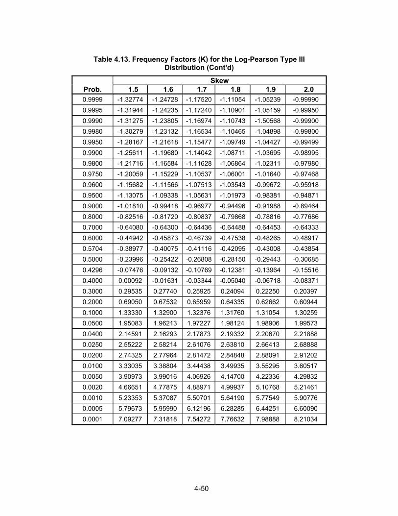
4-50

Table 4.13. Frequency Factors (K) for the Log-Pearson Type III

Distribution (Cont'd)

Skew Prob. 1.5 1.6 1.7 1.8 1.9 2.0 0.9999 -1.32774 -1.24728 -1.17520 -1.11054 -1.05239 -0.99990 0.9995 -1.31944 -1.24235 -1.17240 -1.10901 -1.05159 -0.99950 0.9990 -1.31275 -1.23805 -1.16974 -1.10743 -1.50568 -0.99900 0.9980 -1.30279 -1.23132 -1.16534 -1.10465 -1.04898 -0.99800 0.9950 -1.28167 -1.21618 -1.15477 -1.09749 -1.04427 -0.99499 0.9900 -1.25611 -1.19680 -1.14042 -1.08711 -1.03695 -0.98995 0.9800 -1.21716 -1.16584 -1.11628 -1.06864 -1.02311 -0.97980 0.9750 -1.20059 -1.15229 -1.10537 -1.06001 -1.01640 -0.97468 0.9600 -1.15682 -1.11566 -1.07513 -1.03543 -0.99672 -0.95918 0.9500 -1.13075 -1.09338 -1.05631 -1.01973 -0.98381 -0.94871 0.9000 -1.01810 -0.99418 -0.96977 -0.94496 -0.91988 -0.89464 0.8000 -0.82516 -0.81720 -0.80837 -0.79868 -0.78816 -0.77686 0.7000 -0.64080 -0.64300 -0.64436 -0.64488 -0.64453 -0.64333 0.6000 -0.44942 -0.45873 -0.46739 -0.47538 -0.48265 -0.48917 0.5704 -0.38977 -0.40075 -0.41116 -0.42095 -0.43008 -0.43854 0.5000 -0.23996 -0.25422 -0.26808 -0.28150 -0.29443 -0.30685 0.4296 -0.07476 -0.09132 -0.10769 -0.12381 -0.13964 -0.15516 0.4000 0.00092 -0.01631 -0.03344 -0.05040 -0.06718 -0.08371 0.3000 0.29535 0.27740 0.25925 0.24094 0.22250 0.20397 0.2000 0.69050 0.67532 0.65959 0.64335 0.62662 0.60944 0.1000 1.33330 1.32900 1.32376 1.31760 1.31054 1.30259 0.0500 1.95083 1.96213 1.97227 1.98124 1.98906 1.99573 0.0400 2.14591 2.16293 2.17873 2.19332 2.20670 2.21888 0.0250 2.55222 2.58214 2.61076 2.63810 2.66413 2.68888 0.0200 2.74325 2.77964 2.81472 2.84848 2.88091 2.91202 0.0100 3.33035 3.38804 3.44438 3.49935 3.55295 3.60517 0.0050 3.90973 3.99016 4.06926 4.14700 4.22336 4.29832 0.0020 4.66651 4.77875 4.88971 4.99937 5.10768 5.21461 0.0010 5.23353 5.37087 5.50701 5.64190 5.77549 5.90776 0.0005 5.79673 5.95990 6.12196 6.28285 6.44251 6.60090 0.0001 7.09277 7.31818 7.54272 7.76632 7.98888 8.21034

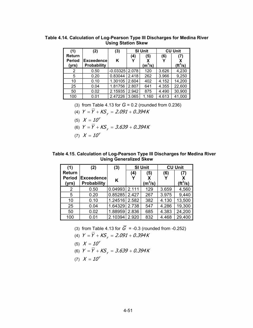
4-51

Table 4.14. Calculation of Log-Pearson Type III Discharges for Medina River

Using Station Skew SI Unit CU Unit (1)

Return Period (yrs)

(2)

Exceedence Probability

(3)

K

(4) Y

(5) X

(m3/s)

(6) Y

(7) X

(ft3/s) 2 0.50 -0.03325 2.078 120 3.626 4,230 5 0.20 0.83044 2.418 262 3.966 9,250 10 0.10 1.30105 2.604 402 4.152 14,200 25 0.04 1.81756 2.807 641 4.355 22,600 50 0.02 2.15935 2.942 875 4.490 30,900 100 0.01 2.47226 3.065 1,160 4.613 41,000

(3) from Table 4.13 for G = 0.2 (rounded from 0.236) (4) K394.0091.2KSYY y +=+=

(5) Y10X = (6) K394.0639.3KSYY y +=+=

(7) Y10X =

Table 4.15. Calculation of Log-Pearson Type III Discharges for Medina River Using Generalized Skew

SI Unit CU Unit (1) Return Period (yrs)

(2)

Exceedence Probability

(3)

K (4) Y

(5) X

(m3/s)

(6) Y

(7) X

(ft3/s) 2 0.50 0.04993 2.111 129 3.659 4,560 5 0.20 0.85285 2.427 267 3.975 9,440 10 0.10 1.24516 2.582 382 4.130 13,500 25 0.04 1.64329 2.738 547 4.286 19,300 50 0.02 1.88959 2.836 685 4.383 24,200 100 0.01 2.10394 2.920 832 4.468 29,400

(3) from Table 4.13 for G = -0.3 (rounded from -0.252)

(4) K394.0091.2KSYY y +=+=

(5) Y10X = (6) K394.0639.3KSYY y +=+=

(7) Y10X =

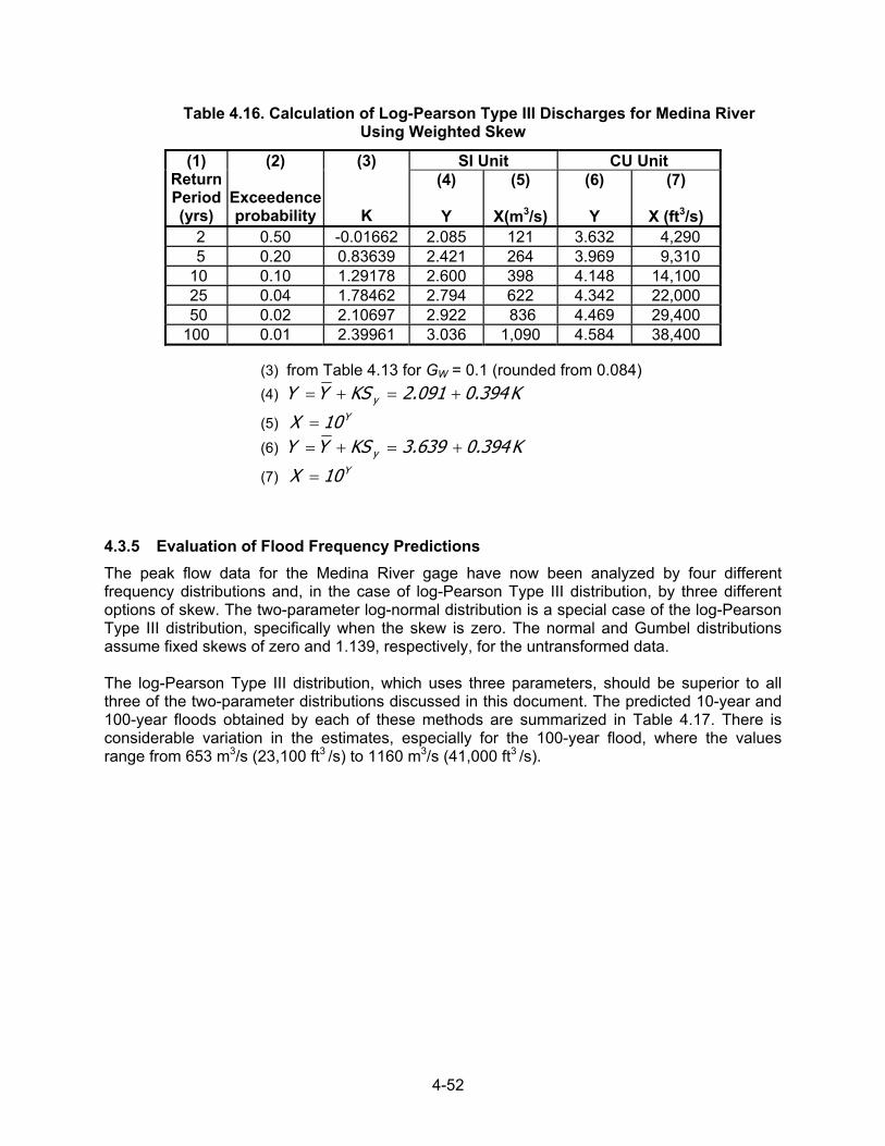
4-52

Table 4.16. Calculation of Log-Pearson Type III Discharges for Medina River Using Weighted Skew

SI Unit CU Unit (1) Return Period (yrs)

(2)

Exceedence probability

(3)

K

(4)

Y

(5)

X(m3/s)

(6)

Y

(7)

X (ft3/s) 2 0.50 -0.01662 2.085 121 3.632 4,290 5 0.20 0.83639 2.421 264 3.969 9,310 10 0.10 1.29178 2.600 398 4.148 14,100 25 0.04 1.78462 2.794 622 4.342 22,000 50 0.02 2.10697 2.922 836 4.469 29,400 100 0.01 2.39961 3.036 1,090 4.584 38,400

(3) from Table 4.13 for GW = 0.1 (rounded from 0.084)

(4) K394.0091.2KSYY y +=+=

(5) Y10X = (6) K394.0639.3KSYY y +=+=

(7) Y10X =

4.3.5 Evaluation of Flood Frequency Predictions The peak flow data for the Medina River gage have now been analyzed by four different frequency distributions and, in the case of log-Pearson Type III distribution, by three different options of skew. The two-parameter log-normal distribution is a special case of the log-Pearson Type III distribution, specifically when the skew is zero. The normal and Gumbel distributions assume fixed skews of zero and 1.139, respectively, for the untransformed data. The log-Pearson Type III distribution, which uses three parameters, should be superior to all three of the two-parameter distributions discussed in this document. The predicted 10-year and 100-year floods obtained by each of these methods are summarized in Table 4.17. There is considerable variation in the estimates, especially for the 100-year flood, where the values range from 653 m3/s (23,100 ft3 /s) to 1160 m3/s (41,000 ft3 /s).

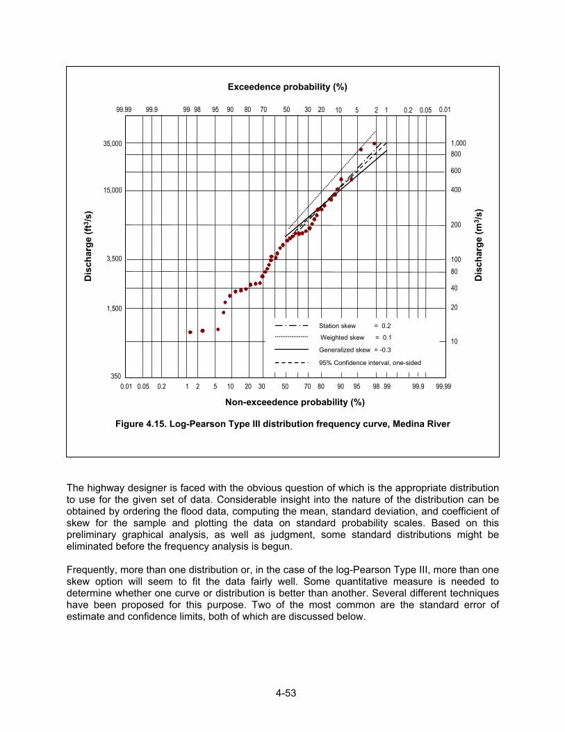
4-53

The highway designer is faced with the obvious question of which is the appropriate distribution to use for the given set of data. Considerable insight into the nature of the distribution can be obtained by ordering the flood data, computing the mean, standard deviation, and coefficient of skew for the sample and plotting the data on standard probability scales. Based on this preliminary graphical analysis, as well as judgment, some standard distributions might be eliminated before the frequency analysis is begun. Frequently, more than one distribution or, in the case of the log-Pearson Type III, more than one skew option will seem to fit the data fairly well. Some quantitative measure is needed to determine whether one curve or distribution is better than another. Several different techniques have been proposed for this purpose. Two of the most common are the standard error of estimate and confidence limits, both of which are discussed below.

Exceedence probability (%)

99.99 99.9 99 98 95 90 80 70 50 30 0.05 0.010.215 21020

99.9999.999989590807050300.050.01 0.2 1 52 10 20

3,500

1,500

35,000

15,000

350

Station skew = 0.2

Weighted skew = 0.1

Generalized skew = -0.3

95% Confidence interval, one-sided

Dis

char

ge (f

t3/s

)

Dis

char

ge (m

3 /s)

1,000800

600

400

200

10080

40

20

10

Non-exceedence probability (%)

Figure 4.15. Log-Pearson Type III distribution frequency curve, Medina River

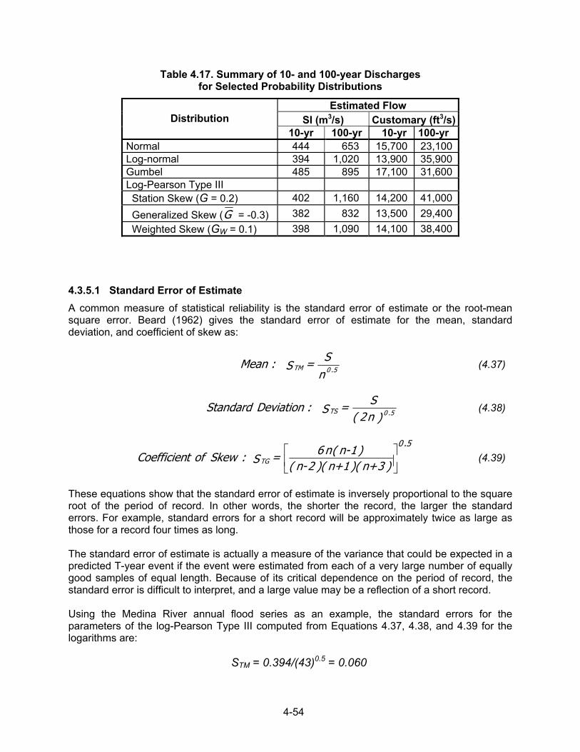
4-54

Table 4.17. Summary of 10- and 100-year Discharges for Selected Probability Distributions

Estimated Flow SI (m3/s) Customary (ft3/s) Distribution

10-yr 100-yr 10-yr 100-yr Normal 444 653 15,700 23,100 Log-normal 394 1,020 13,900 35,900 Gumbel 485 895 17,100 31,600 Log-Pearson Type III Station Skew (G = 0.2) 402 1,160 14,200 41,000 Generalized Skew (G = -0.3) 382 832 13,500 29,400 Weighted Skew (GW = 0.1) 398 1,090 14,100 38,400

4.3.5.1 Standard Error of Estimate A common measure of statistical reliability is the standard error of estimate or the root-mean square error. Beard (1962) gives the standard error of estimate for the mean, standard deviation, and coefficient of skew as:

nS = S :Mean 5.0TM (4.37)

)n2(

S = S :Deviation Standard 5.0TS (4.38)

)3n+)(1n+)(2n-(

)1n-(n6 = S :Skew of tCoefficien5.0

TG (4.39)

These equations show that the standard error of estimate is inversely proportional to the square root of the period of record. In other words, the shorter the record, the larger the standard errors. For example, standard errors for a short record will be approximately twice as large as those for a record four times as long. The standard error of estimate is actually a measure of the variance that could be expected in a predicted T-year event if the event were estimated from each of a very large number of equally good samples of equal length. Because of its critical dependence on the period of record, the standard error is difficult to interpret, and a large value may be a reflection of a short record. Using the Medina River annual flood series as an example, the standard errors for the parameters of the log-Pearson Type III computed from Equations 4.37, 4.38, and 4.39 for the logarithms are:

STM = 0.394/(43)0.5 = 0.060

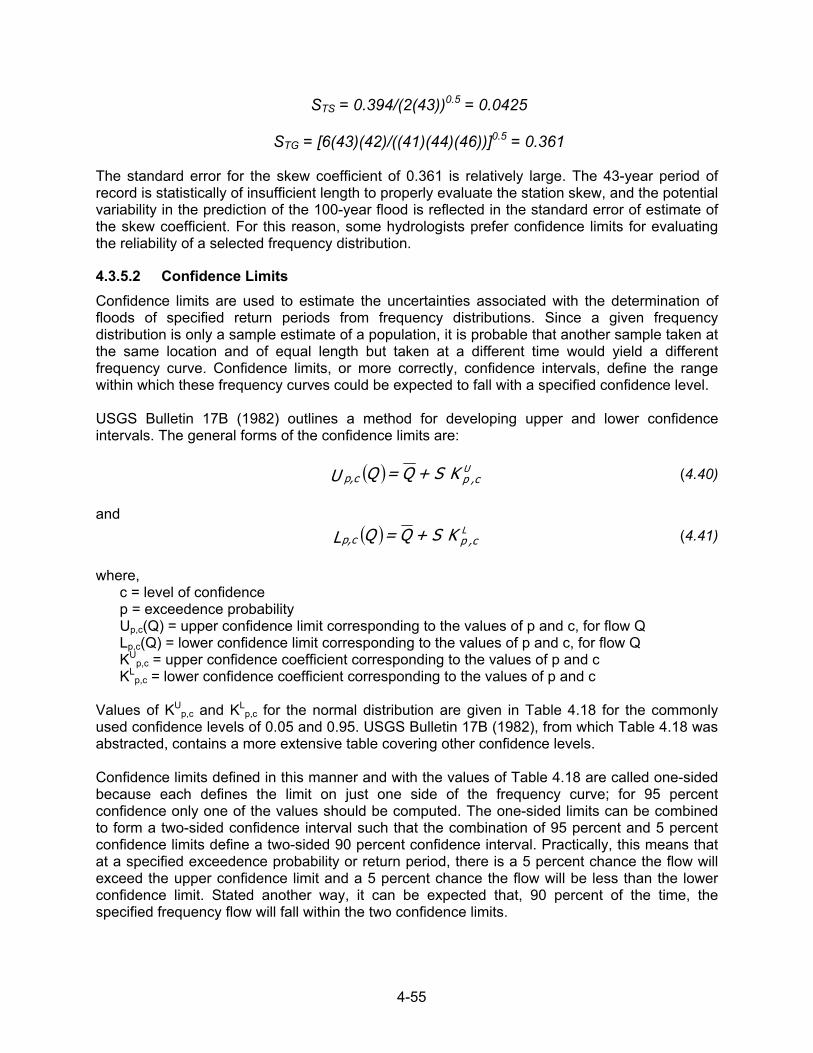
4-55

STS = 0.394/(2(43))0.5 = 0.0425

STG = [6(43)(42)/((41)(44)(46))]0.5 = 0.361 The standard error for the skew coefficient of 0.361 is relatively large. The 43-year period of record is statistically of insufficient length to properly evaluate the station skew, and the potential variability in the prediction of the 100-year flood is reflected in the standard error of estimate of the skew coefficient. For this reason, some hydrologists prefer confidence limits for evaluating the reliability of a selected frequency distribution.

4.3.5.2 Confidence Limits Confidence limits are used to estimate the uncertainties associated with the determination of floods of specified return periods from frequency distributions. Since a given frequency distribution is only a sample estimate of a population, it is probable that another sample taken at the same location and of equal length but taken at a different time would yield a different frequency curve. Confidence limits, or more correctly, confidence intervals, define the range within which these frequency curves could be expected to fall with a specified confidence level. USGS Bulletin 17B (1982) outlines a method for developing upper and lower confidence intervals. The general forms of the confidence limits are: ( ) U

c,pcp, K S + Q = QU (4.40) and ( ) L

c,pcp, K S + Q = QL (4.41) where, c = level of confidence p = exceedence probability Up,c(Q) = upper confidence limit corresponding to the values of p and c, for flow Q Lp,c(Q) = lower confidence limit corresponding to the values of p and c, for flow Q KU

p,c = upper confidence coefficient corresponding to the values of p and c KL

p,c = lower confidence coefficient corresponding to the values of p and c Values of KU

p,c and KLp,c for the normal distribution are given in Table 4.18 for the commonly

used confidence levels of 0.05 and 0.95. USGS Bulletin 17B (1982), from which Table 4.18 was abstracted, contains a more extensive table covering other confidence levels. Confidence limits defined in this manner and with the values of Table 4.18 are called one-sided because each defines the limit on just one side of the frequency curve; for 95 percent confidence only one of the values should be computed. The one-sided limits can be combined to form a two-sided confidence interval such that the combination of 95 percent and 5 percent confidence limits define a two-sided 90 percent confidence interval. Practically, this means that at a specified exceedence probability or return period, there is a 5 percent chance the flow will exceed the upper confidence limit and a 5 percent chance the flow will be less than the lower confidence limit. Stated another way, it can be expected that, 90 percent of the time, the specified frequency flow will fall within the two confidence limits.

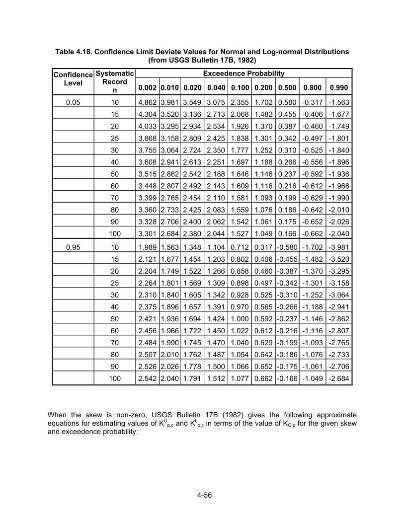
4-56

Table 4.18. Confidence Limit Deviate Values for Normal and Log-normal Distributions (from USGS Bulletin 17B, 1982)

Exceedence Probability Confidence Level

Systematic Record

n 0.002

0.010

0.020

0.040

0.100

0.200

0.500

0.800

0.990

0.05

10

4.862

3.981

3.549

3.075

2.355

1.702

0.580

-0.317

-1.563

15 4.304

3.520

3.136

2.713

2.068

1.482

0.455

-0.406

-1.677

20 4.033

3.295

2.934

2.534

1.926

1.370

0.387

-0.460

-1.749

25 3.868

3.158

2.809

2.425

1.838

1.301

0.342

-0.497

-1.801

30 3.755

3.064

2.724

2.350

1.777

1.252

0.310

-0.525

-1.840

40 3.608

2.941

2.613

2.251

1.697

1.188

0.266

-0.556

-1.896

50 3.515

2.862

2.542

2.188

1.646

1.146

0.237

-0.592

-1.936

60 3.448

2.807

2.492

2.143

1.609

1.116

0.216

-0.612

-1.966

70 3.399

2.765

2.454

2.110

1.581

1.093

0.199

-0.629

-1.990

80 3.360

2.733

2.425

2.083

1.559

1.076

0.186

-0.642

-2.010

90 3.328

2.706

2.400

2.062

1.542

1.061

0.175

-0.652

-2.026

100 3.301

2.684

2.380

2.044

1.527

1.049

0.166

-0.662

-2.040

0.95

10

1.989

1.563

1.348

1.104

0.712

0.317

-0.580

-1.702

-3.981

15 2.121

1.677

1.454

1.203

0.802

0.406

-0.455

-1.482

-3.520

20 2.204

1.749

1.522

1.266

0.858

0.460

-0.387

-1.370

-3.295

25 2.264

1.801

1.569

1.309

0.898

0.497

-0.342

-1.301

-3.158

30 2.310

1.840

1.605

1.342

0.928

0.525

-0.310

-1.252

-3.064

40 2.375

1.896

1.657

1.391

0.970

0.565

-0.266

-1.188

-2.941

50 2.421

1.936

1.694

1.424

1.000

0.592

-0.237

-1.146

-2.862

60 2.456

1.966

1.722

1.450

1.022

0.612

-0.216

-1.116

-2.807

70 2.484

1.990

1.745

1.470

1.040

0.629

-0.199

-1.093

-2.765

80 2.507

2.010

1.762

1.487

1.054

0.642

-0.186

-1.076

-2.733

90 2.526

2.026

1.778

1.500

1.066

0.652

-0.175

-1.061

-2.706

100 2.542

2.040

1.791

1.512

1.077

0.662

-0.166

-1.049

-2.684

When the skew is non-zero, USGS Bulletin 17B (1982) gives the following approximate equations for estimating values of KU

p,c and KLp,c in terms of the value of KG,p for the given skew

and exceedence probability:

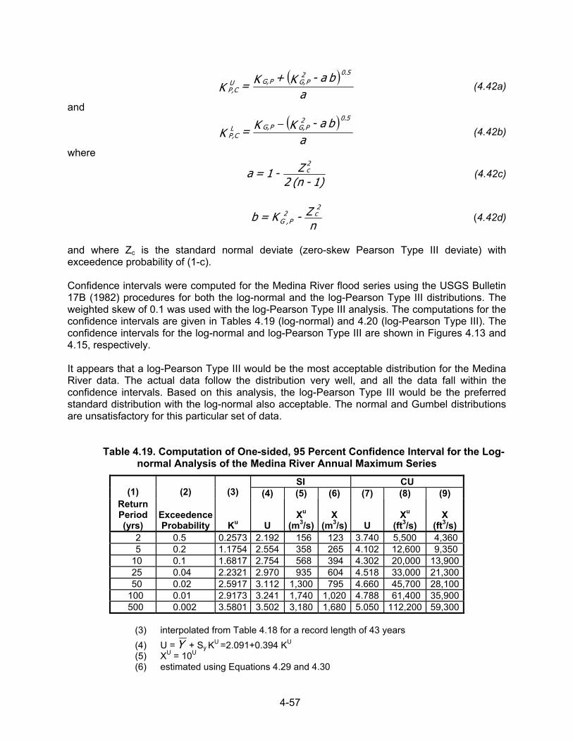
4-57

( )

aba - K + K = K

5.02PG,PG,U

CP, (4.42a)

and

( )

aba - K K = K

5.02PG,PG,L

CP,−

(4.42b)

where

1) - (n2

Z - 1 = a2c (4.42c)

n

Z - K = b2

c2P,G (4.42d)

and where Zc is the standard normal deviate (zero-skew Pearson Type III deviate) with exceedence probability of (1-c). Confidence intervals were computed for the Medina River flood series using the USGS Bulletin 17B (1982) procedures for both the log-normal and the log-Pearson Type III distributions. The weighted skew of 0.1 was used with the log-Pearson Type III analysis. The computations for the confidence intervals are given in Tables 4.19 (log-normal) and 4.20 (log-Pearson Type III). The confidence intervals for the log-normal and log-Pearson Type III are shown in Figures 4.13 and 4.15, respectively. It appears that a log-Pearson Type III would be the most acceptable distribution for the Medina River data. The actual data follow the distribution very well, and all the data fall within the confidence intervals. Based on this analysis, the log-Pearson Type III would be the preferred standard distribution with the log-normal also acceptable. The normal and Gumbel distributions are unsatisfactory for this particular set of data. Table 4.19. Computation of One-sided, 95 Percent Confidence Interval for the Log-

normal Analysis of the Medina River Annual Maximum Series SI CU

(1) (2) (3) (4) (5) (6) (7) (8) (9) Return Period (yrs)

Exceedence Probability Ku U

Xu (m3/s)

X (m3/s) U

Xu (ft3/s)

X (ft3/s)

2 0.5 0.2573 2.192 156 123 3.740 5,500 4,360 5 0.2 1.1754 2.554 358 265 4.102 12,600 9,350 10 0.1 1.6817 2.754 568 394 4.302 20,000 13,900 25 0.04 2.2321 2.970 935 604 4.518 33,000 21,300 50 0.02 2.5917 3.112 1,300 795 4.660 45,700 28,100 100 0.01 2.9173 3.241 1,740 1,020 4.788 61,400 35,900 500 0.002 3.5801 3.502 3,180 1,680 5.050 112,200 59,300

(3) interpolated from Table 4.18 for a record length of 43 years (4) U = Y + Sy KU =2.091+0.394 KU (5) XU = 10U (6) estimated using Equations 4.29 and 4.30

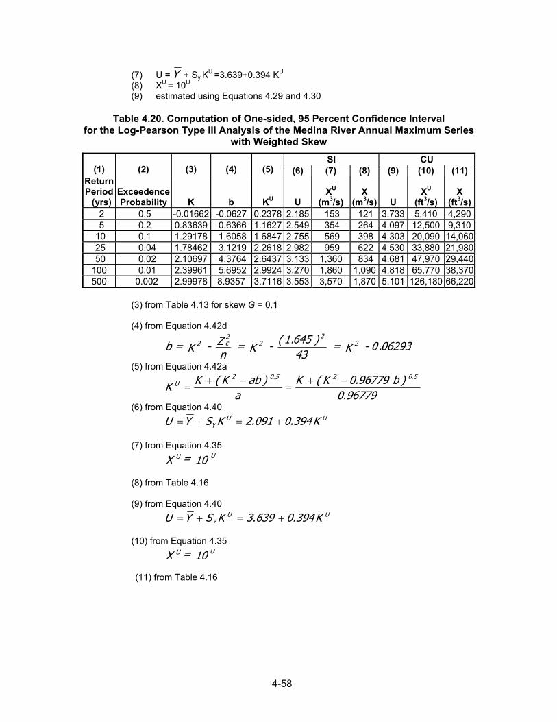
4-58

(7) U = Y + Sy KU =3.639+0.394 KU (8) XU = 10U (9) estimated using Equations 4.29 and 4.30

Table 4.20. Computation of One-sided, 95 Percent Confidence Interval

for the Log-Pearson Type III Analysis of the Medina River Annual Maximum Series with Weighted Skew

SI CU (1) (2) (3) (4) (5) (6) (7) (8) (9) (10) (11)

Return Period (yrs)

Exceedence Probability K b KU U

XU

(m3/s) X

(m3/s) U XU

(ft3/s) X

(ft3/s) 2 0.5 -0.01662 -0.0627 0.2378 2.185 153 121 3.733 5,410 4,290 5 0.2 0.83639 0.6366 1.1627 2.549 354 264 4.097 12,500 9,310 10 0.1 1.29178 1.6058 1.6847 2.755 569 398 4.303 20,090 14,060 25 0.04 1.78462 3.1219 2.2618 2.982 959 622 4.530 33,880 21,980 50 0.02 2.10697 4.3764 2.6437 3.133 1,360 834 4.681 47,970 29,440100 0.01 2.39961 5.6952 2.9924 3.270 1,860 1,090 4.818 65,770 38,370500 0.002 2.99978 8.9357 3.7116 3.553 3,570 1,870 5.101 126,180 66,220

(3) from Table 4.13 for skew G = 0.1 (4) from Equation 4.42d

06293.0 - K = 43

)645.1( - K = nZ - Kb = 2

22

2c2

(5) from Equation 4.42a

96779.0)b 96779.0K(K

a)abK(KK

5.025.02U −+

=−+

=

(6) from Equation 4.40 UU

Y K394.0091.2KSYU +=+=

(7) from Equation 4.35 10= X UU

(8) from Table 4.16 (9) from Equation 4.40 UU

Y K394.0639.3KSYU +=+= (10) from Equation 4.35 10= X UU (11) from Table 4.16

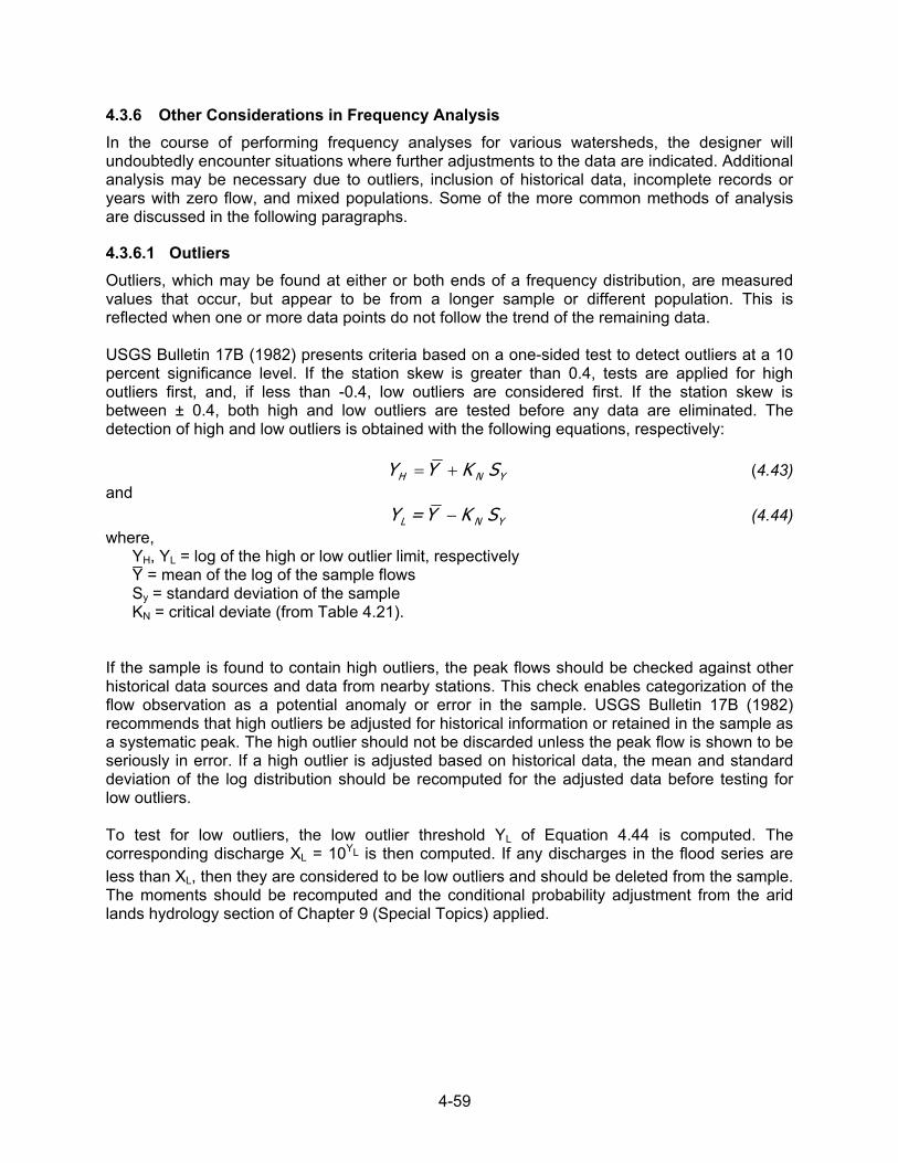
4-59

4.3.6 Other Considerations in Frequency Analysis In the course of performing frequency analyses for various watersheds, the designer will undoubtedly encounter situations where further adjustments to the data are indicated. Additional analysis may be necessary due to outliers, inclusion of historical data, incomplete records or years with zero flow, and mixed populations. Some of the more common methods of analysis are discussed in the following paragraphs.

4.3.6.1 Outliers Outliers, which may be found at either or both ends of a frequency distribution, are measured values that occur, but appear to be from a longer sample or different population. This is reflected when one or more data points do not follow the trend of the remaining data. USGS Bulletin 17B (1982) presents criteria based on a one-sided test to detect outliers at a 10 percent significance level. If the station skew is greater than 0.4, tests are applied for high outliers first, and, if less than -0.4, low outliers are considered first. If the station skew is between ± 0.4, both high and low outliers are tested before any data are eliminated. The detection of high and low outliers is obtained with the following equations, respectively: YNH SKYY += (4.43) and YNL SKY = Y − (4.44) where, YH, YL = log of the high or low outlier limit, respectively Y = mean of the log of the sample flows Sy = standard deviation of the sample KN = critical deviate (from Table 4.21). If the sample is found to contain high outliers, the peak flows should be checked against other historical data sources and data from nearby stations. This check enables categorization of the flow observation as a potential anomaly or error in the sample. USGS Bulletin 17B (1982) recommends that high outliers be adjusted for historical information or retained in the sample as a systematic peak. The high outlier should not be discarded unless the peak flow is shown to be seriously in error. If a high outlier is adjusted based on historical data, the mean and standard deviation of the log distribution should be recomputed for the adjusted data before testing for low outliers. To test for low outliers, the low outlier threshold YL of Equation 4.44 is computed. The corresponding discharge XL = 10YL is then computed. If any discharges in the flood series are less than XL, then they are considered to be low outliers and should be deleted from the sample. The moments should be recomputed and the conditional probability adjustment from the arid lands hydrology section of Chapter 9 (Special Topics) applied.

4-60

Table 4.21. Outlier Test Deviates (KN) at 10 Percent Significance Level (from USGS Bulletin 17B, 1982)

Sample Size

KN Value

Sample Size

KN Value

Sample Size

KN Value

Sample Size

KN Value

10 2.036 45 2.727 80 2.940 115 3.064 11 2.088 46 2.736 81 2.945 116 3.067 12 2.134 47 2.744 82 2.949 117 3.070 13 2.165 48 2.753 83 2.953 118 3.073 14 2.213 49 2.760 84 2.957 119 3.075 15 2.247 50 2.768 85 2.961 120 3.078 16 2.279 51 2.775 86 2.966 121 3.081 17 2.309 52 2.783 87 2.970 122 3.083 18 2.335 53 2.790 88 2.973 123 3.086 19 2.361 54 2.798 89 2.977 124 3.089 20 2.385 55 2.804 90 2.989 125 3.092 21 2.408 56 2.811 91 2.984 126 3.095 22 2.429 57 2.818 92 2.889 127 3.097 23 2.448 58 2.824 93 2.993 128 3.100 24 2.467 59 2.831 94 2.996 129 3.102 25 2.487 60 2.837 95 3.000 130 3.104 26 2.502 61 2.842 96 3.003 131 3.107 27 2.510 62 2.849 97 3.006 132 3.109 28 2.534 63 2.854 98 3.011 133 3.112 29 2.549 64 2.860 99 3.014 134 3.114 30 2.563 65 2.866 100 3.017 135 3.116 31 2.577 66 2.871 101 3.021 136 3.119 32 2.591 67 2.877 102 3.024 137 3.122 33 2.604 68 2.883 103 3.027 138 3.124 34 2.616 69 2.888 104 3.030 139 3.126 35 2.628 70 2.893 105 3.033 140 3.129 36 2.639 71 2.897 106 3.037 141 3.131 37 2.650 72 2.903 107 3.040 142 3.133 38 2.661 73 2.908 108 3.043 143 3.135 39 2.671 74 2.912 109 3.046 144 3.138 40 2.682 75 2.917 110 3.049 145 3.140 41 2.692 76 2.922 111 3.052 146 3.142 42 2.700 77 2.927 112 3.055 147 3.144 43 2.710 78 2.931 113 3.058 148 3.146 44 2.720 79 2.935 114 3.061 149 3.148

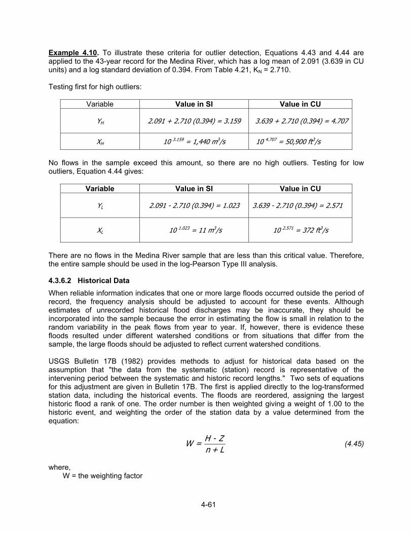
4-61

Example 4.10. To illustrate these criteria for outlier detection, Equations 4.43 and 4.44 are applied to the 43-year record for the Medina River, which has a log mean of 2.091 (3.639 in CU units) and a log standard deviation of 0.394. From Table 4.21, KN = 2.710. Testing first for high outliers:

Variable Value in SI Value in CU

YH

2.091 + 2.710 (0.394) = 3.159

3.639 + 2.710 (0.394) = 4.707

XH 10 3.159 = 1,440 m3/s 10 4.707 = 50,900 ft3/s

No flows in the sample exceed this amount, so there are no high outliers. Testing for low outliers, Equation 4.44 gives:

Variable Value in SI Value in CU

YL

2.091 - 2.710 (0.394) = 1.023

3.639 - 2.710 (0.394) = 2.571

XL

10 1.023 = 11 m3/s

10 2.571 = 372 ft3/s

There are no flows in the Medina River sample that are less than this critical value. Therefore, the entire sample should be used in the log-Pearson Type III analysis.

4.3.6.2 Historical Data When reliable information indicates that one or more large floods occurred outside the period of record, the frequency analysis should be adjusted to account for these events. Although estimates of unrecorded historical flood discharges may be inaccurate, they should be incorporated into the sample because the error in estimating the flow is small in relation to the random variability in the peak flows from year to year. If, however, there is evidence these floods resulted under different watershed conditions or from situations that differ from the sample, the large floods should be adjusted to reflect current watershed conditions. USGS Bulletin 17B (1982) provides methods to adjust for historical data based on the assumption that "the data from the systematic (station) record is representative of the intervening period between the systematic and historic record lengths." Two sets of equations for this adjustment are given in Bulletin 17B. The first is applied directly to the log-transformed station data, including the historical events. The floods are reordered, assigning the largest historic flood a rank of one. The order number is then weighted giving a weight of 1.00 to the historic event, and weighting the order of the station data by a value determined from the equation:

L + nZ-H = W (4.45)

where, W = the weighting factor

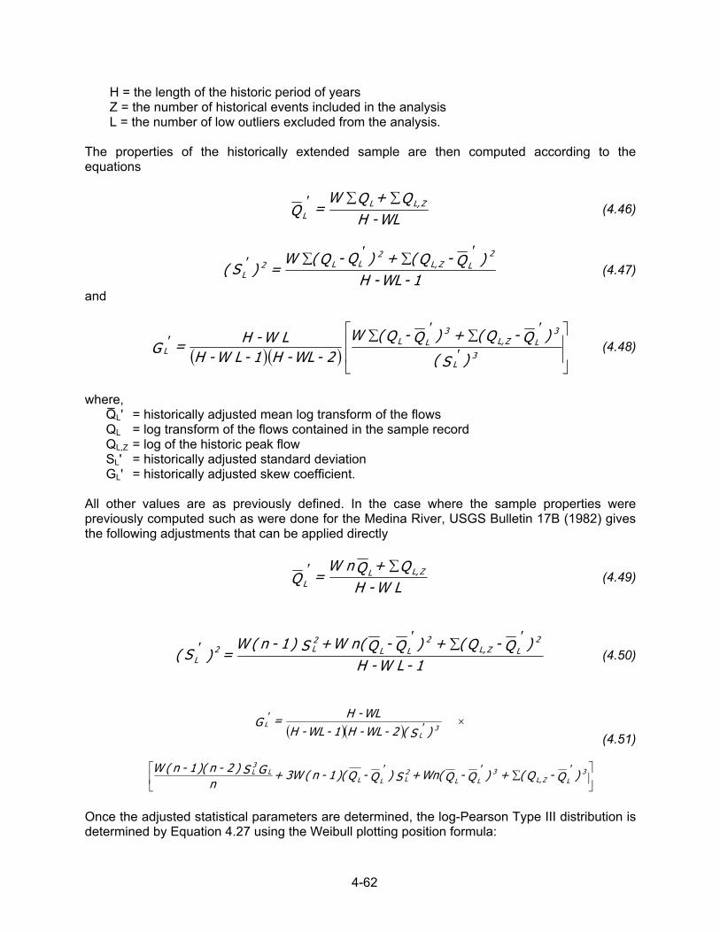
4-62

H = the length of the historic period of years Z = the number of historical events included in the analysis L = the number of low outliers excluded from the analysis. The properties of the historically extended sample are then computed according to the equations

WL - H

Q+QW =Q ZL,L

L

∑∑′ (4.46)

1- WL - H

)Q - Q( + )Q - Q(W = )S(

2LZL,

2LL2

L

′∑′∑′ (4.47)

and

( )( )

′

′∑′∑′3

L

3LZL,

3LL

L)S(

)Q -Q( + )Q -Q(W

2-WL-H1-LW-HLW-H = G (4.48)

where, QL' = historically adjusted mean log transform of the flows QL = log transform of the flows contained in the sample record QL,Z = log of the historic peak flow SL' = historically adjusted standard deviation GL' = historically adjusted skew coefficient. All other values are as previously defined. In the case where the sample properties were previously computed such as were done for the Medina River, USGS Bulletin 17B (1982) gives the following adjustments that can be applied directly

LW - HQ + QnW

= Q ZL,LL

∑′ (4.49)

1 - LW - H

)Q - Q( + )Q - Q(nW + S )1- n(W = )S(

2LZL,

2LL

2L2

L

′∑′′ (4.50)

( )( )

′∑′′

×′′

3LZL,

3LL

2LLL

L3L

3L

L

)Q-Q( +)Q-QWn( +S)Q-Q)(1-n(W3 +n

GS)2-n)(1-n(W

)S(2 - WL - H1 - WL - H

WL - H = G (4.51)

Once the adjusted statistical parameters are determined, the log-Pearson Type III distribution is determined by Equation 4.27 using the Weibull plotting position formula:

4-63

1 + H

m = P′

(4.52)

where m´ is the adjusted rank order number of the floods including historical events, where

m´ = m for 1 ≤ m ≤ Z

m´ = Wm - (W - 1)(Z + 0.5) for (Z + 1) ≤ m ≤ (Z + nL) Detailed examples illustrating the computations for the historic adjustment are contained in USGS Bulletin 17B (1982) and the designer should consult this reference for further information.

4.3.6.3 Incomplete Records and Zero Flows Stream flow records are often interrupted for a variety of reasons. Gages may be removed for some period of time, there may be periods of zero flow that are common in the arid regions of the United States, and there may be periods when a gage is inoperative either because the flow is too low to record or it is too large and causes a gage malfunction. If the break in the record is not flood related, such as the removal of a gage, no special adjustments are needed and the segments of the interrupted record can be combined together to produce a record equal to the sum of the length of the segments. When a gage malfunctions during a flood, it is usually possible to estimate the peak discharge from highwater marks or slope-area calculations. The estimate is made a part of the record, and a frequency analysis performed without further adjustment. Zero flows or flows that are too low to be recorded present more of a problem because, in the log transform, these flows produce undefined values. In this case, USGS Bulletin 17B (1982) presents an adjustment based on conditional probability that is applicable if not more than 25 percent of the sample is eliminated. The adjustment for zero flows also is applied only after all other data adjustments have been made. The adjustment is made by first calculating the relative frequency, Pa, that the annual peak will exceed the level below where either flows are zero or not considered (the truncation level):

nM = P a (4.53)

where M is the number of flows above the truncated level and n is the total period of record. The exceedence probabilities, P, of selected points on the frequency curve are recomputed as a conditional probability as follows da PPP = (4.54) where Pd is the selected probability. Since the frequency curve adjusted by Equation 4.54 has unknown statistics, its properties, synthetic values, are computed by the equations:

4-64

)S(K-)Qlog( = Q S50.050.0s (4.55)

K - K

)Q/Qlog( = S

50.001.0

50.001.0S (4.56)

and

( )( )

Q/QlogQ/Qlog

12.3 + 50.2 = -G50.010.0

10.001.0S (4.57)

where Qs, Ss, and Gs are the mean, standard deviation, and skew of the synthetic frequency curve, Q0.01, Q0.10, and Q0.50 are discharges with exceedence probabilities of 0.01, 0.10 and 0.50, respectively, and K0.01 and K0.50 are the log-Pearson Type III deviates for exceedence probabilities of 0.01 and 0.50, respectively. The values of Q0.01, Q0.10 and Q0.50 must usually be interpolated since probabilities computed with Equation 4.53 are not normally those needed to compute the properties of the synthetic or truncated distribution. The log-Pearson Type III distribution can then be computed in the conventional manner using the synthetic statistical properties. USGS Bulletin 17B (1982) recommends the distribution be compared with the observed flows since data adjusted for conditional probability may not follow a log-Pearson Type III distribution.

4.3.6.4 Mixed Populations In some areas of the United States, floods are caused by combinations of events (e.g., rainfall and snowmelt in mountainous areas or rainfall and hurricane events along the Gulf and Atlantic coasts). Records from such combined events are said to be mixed populations. These records are often characterized by very large skew coefficients and, when plotted, suggest that two different distributions might be applicable. Such records should be divided into two separate records according to their respective causes, with each record analyzed separately by an appropriate frequency distribution. The two separate frequency curves can then be combined through the concept of the addition of the probabilities of two events as follows: ( ) ( ) ( ) ( ) ( )QPrQPr - QPr + QPr = Q or Q Pr mmm (4.58)

4.3.6.5 Two-Station Comparison The objective of this method is to improve the mean and standard deviation of the logarithms at a short-record station (Y) using the statistics from a nearby long-record station (X). The method is from Appendix 7 of USGS Bulletin 17B (1982). The steps of the procedure depend on the nature of the records. Specifically, there are two cases: (1) the entire short record occurred during the duration of the long-record station, and (2) only part of the short record occurred during the duration of the long-record station. The following notation applies to the procedure:

Nx = record length at long-record station

N1 = number of years when flows were concurrently observed at X and Y

4-65

N2 = number of years when flows were observed at the long-record station, but not

observed at the short-record station N3 = record length at short-record station

Sy = Standard deviation of the logarithm of flows for the extended period at the short-

record station

Sx1 = Standard deviation of logarithm of flows at the long-record station during the concurrent period

Sx2 = Standard deviation of logarithm of flows at the long-record station for the period

when flows were not observed at the short-record station Sy1 = Standard deviation of the logarithm of flows at the short-record station for the

concurrent period

Sy3 = Standard deviation of logarithm of flows for the entire period at the short-record station

X1 = Logarithms of flows for the long-record station during the concurrent period

X1 = Mean logarithm of flows at the long-record station for the concurrent period

X2 = Mean logarithm of flows at the long-record station for the period when flow

records are not available at the short-record station

X3 = Mean logarithm of flows for the entire period at the long-record station

Y1 = Logarithms of flows for the short-record station during the concurrent period

Y = Mean logarithm of flows for the extended period at the short-record station

Y1 = Mean logarithm of flows for the period of observed flow at the short-record station (concurrent period)

Y3 = Mean logarithm of flows for the entire period at the short-record station

Case 1 is where N1 equals N3. Case 2 is where N3 is greater than N1.

The following procedure is used:

1a. Compute the regression coefficient, b:

( ) N/X - X

N/YX- YXb = 1

21

21

11111

∑∑∑∑∑ (4.59)

1b. Compute the correlation coefficient, r:

4-66

SSb = r

y

x

1

1 (4.60)

2. If Case 1 applies, go to Step 4; however, if case 2 applies, begin at Step 3.

3a. Compute the variance of the adjusted mean (Y):

( )

)3 - N()r - 1( - r

N + NN - 1

N)S(

= YVar1

22

21

2

1

2y 1 (4.61)

3b. Compute Sy3

2:

23i

N

1i=3

23y )Y -Y(1 - N

1 = S3

∑ (4.62)

3c. Compute the variance of the mean Y3 of the entire record at the short-record station:

( ) ( )N

S = Yvar3

2y

33 (4.63)

3d. Compare Var(Y) and Var(Y3). If Var(Y) < Var(Y3), then go to Step 4; otherwise, go to

Step 3e. 3e. Compute Y3, which should be used as the best estimate of the mean:

YN1 = Y i

N

1i=33

3

∑ (4.64)

3f. Go to Step 5.

4a. Compute the critical correlation coefficient rc:

( ) 5.0

1c 2N

1 = r−

(4.65)

4b. If r > rc, then adjust the mean:

( )[ ]1221

21 XXb

N + NN + Y = Y − (4.66a)

or

( )131 XXbY = Y −+ (4.66b)

4-67

and go to Step 5.

4c. If r < rc, use Y1 for Case 1 or Y3 for Case 2 and go to Step 5.

5. If Case 1 applies, then go to Step 7; however, if Case 2 applies, begin at Step 6. 6a. Compute the variance of the adjusted variance Sy

2:

] + CBr + Ar[ )1 - N + N(

)S(N +

1 - N

)S(2 = )S(Var 24

221

4y2

1

4y2

y11 (4.67)

where:

( ) ( )( )( )

( )( )

( )( )

( )( )( )

( )( ) ( )2-N3-N

4-NNN + 3-N

1+N4-N2 + 3-N

4-NN2+

1-N2-N+N21+N -

5-N3-N2+N3 +

3-N1+N2C =

)2-(N)3-N()4-N(NN2 -

)3-N()3+N)(4-N(2-

)3-N()5-N)(4-N(N2 +

)3-N()14-N-N(2 +

)5-N()3-N()6-N()2+N(6B =

)3 - N()4 - N(4 +

)2 - N()3 - N()4 - N(NN+

)3 - N()4 - N(N2 -

)3 - N()4 - N(8 -

)5 - N()3 - N()8 - N()6 - N()2 + N(A =

12

1

2121

1

112

1

12

1

211

11

2

1

1

12

1

2121

1

11

21

112

1

12

1

11

12

1

1

12

1

2121

21

212

1

1

11

112

(4.68)

6b. Compute the variance of the variance (Sy3

2) of the entire record at the short-record station:

( ) ( )1 - N

S2 = SVar3

23Y2

3Y (4.69)

6c. If Var(Sy3

2) > Var(Sy2), go to Step 7; otherwise, go to Step 6d.

6d. Use Sy3 as the best estimate of the standard deviation.

6e. Go to Step 8.

7a. Compute the critical correlation coefficient ra:

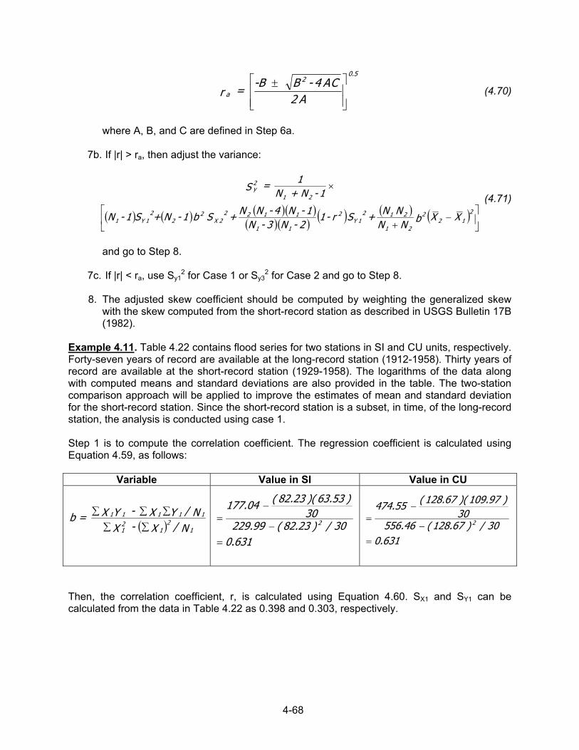
4-68

±A2

CA4-B -B = r

25.0

a (4.70)

where A, B, and C are defined in Step 6a.

7b. If |r| > ra, then adjust the variance:

( ) ( ) ( )( )( )( ) ( ) ( ) ( )

−

+

×

212

2

21

2121Y

2

11

11222X

22

21Y1

21

2y

XXbNNNN+Sr-1

2-N3-N1-N4-NN+Sb1-N+S1-N

1- + NN1 = S

(4.71)

and go to Step 8.

7c. If |r| < ra, use Sy1

2 for Case 1 or Sy32 for Case 2 and go to Step 8.

8. The adjusted skew coefficient should be computed by weighting the generalized skew

with the skew computed from the short-record station as described in USGS Bulletin 17B (1982).

Example 4.11. Table 4.22 contains flood series for two stations in SI and CU units, respectively. Forty-seven years of record are available at the long-record station (1912-1958). Thirty years of record are available at the short-record station (1929-1958). The logarithms of the data along with computed means and standard deviations are also provided in the table. The two-station comparison approach will be applied to improve the estimates of mean and standard deviation for the short-record station. Since the short-record station is a subset, in time, of the long-record station, the analysis is conducted using case 1. Step 1 is to compute the correlation coefficient. The regression coefficient is calculated using Equation 4.59, as follows:

Variable Value in SI Value in CU

( ) N/X - XN/YX - YXb =

12

121

11111

∑∑∑∑∑

631.030/)23.82(99.229

30)53.63)(23.82(04.177

2

=−

−=

631.0

30/)67.128(46.55630

)97.109)(67.128(55.4742

=−

−=

Then, the correlation coefficient, r, is calculated using Equation 4.60. SX1 and SY1 can be calculated from the data in Table 4.22 as 0.398 and 0.303, respectively.

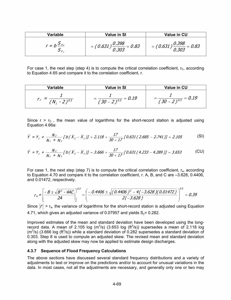
4-69

Variable Value in SI Value in CU

SSb = r

y

x

1

1 83.0303.0398.0)631.0( == 83.0

303.0398.0)631.0( ==

For case 1, the next step (step 4) is to compute the critical correlation coefficient, rC, according to Equation 4.65 and compare it to the correlation coefficient, r.

Variable Value in SI Value in CU

5.01

c )2 - N(1 = r 19.0

)230(1

5.0 =−

= 19.0)230(

15.0 =

−=

Since r > rC , the mean value of logarithms for the short-record station is adjusted using Equation 4.66a:

105.2)]741.2685.2(631.0[1730

17118.2)]XX(b[N + N

N + = YY 1221

21 =−

++=− (SI)

653.3)]289.4233.4(631.0[

173017666.3)]XX(b[

N + NN + = YY 12

21

21 =−

++=− (CU)

For case 1, the next step (step 7) is to compute the critical correlation coefficient, ra, according to Equation 4.70 and compare it to the correlation coefficient, r. A, B, and C are –3.628, 0.4406, and 0.01472, respectively.

39.0)628.3(2

)01472.0)(628.3(4)4406.0(4406.02A

4AC-B B- = r

5.022

5.0

a =

−−−±−

=

±

Since r > ra, the variance of logarithms for the short-record station is adjusted using Equation 4.71, which gives an adjusted variance of 0.07957 and yields Sy= 0.282. Improved estimates of the mean and standard deviation have been developed using the long-record data. A mean of 2.105 log (m3/s) (3.653 log (ft3/s)) supersedes a mean of 2.118 log (m3/s) (3.666 log (ft3/s)) while a standard deviation of 0.282 supersedes a standard deviation of 0.303. Step 8 is used to compute an adjusted skew. The revised mean and standard deviation along with the adjusted skew may now be applied to estimate design discharges.

4.3.7 Sequence of Flood Frequency Calculations The above sections have discussed several standard frequency distributions and a variety of adjustments to test or improve on the predictions and/or to account for unusual variations in the data. In most cases, not all the adjustments are necessary, and generally only one or two may

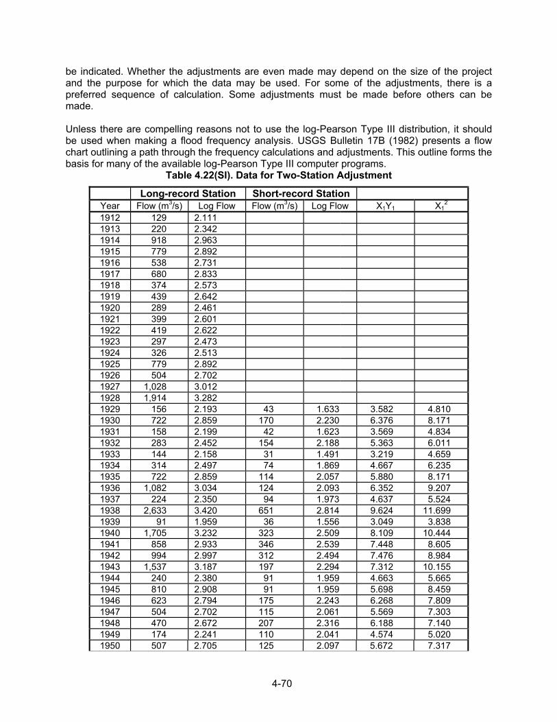
4-70

be indicated. Whether the adjustments are even made may depend on the size of the project and the purpose for which the data may be used. For some of the adjustments, there is a preferred sequence of calculation. Some adjustments must be made before others can be made. Unless there are compelling reasons not to use the log-Pearson Type III distribution, it should be used when making a flood frequency analysis. USGS Bulletin 17B (1982) presents a flow chart outlining a path through the frequency calculations and adjustments. This outline forms the basis for many of the available log-Pearson Type III computer programs.

Table 4.22(SI). Data for Two-Station Adjustment

Long-record Station Short-record Station Year Flow (m3/s) Log Flow Flow (m3/s) Log Flow X1Y1 X1

2 1912 129 2.111 1913 220 2.342 1914 918 2.963 1915 779 2.892 1916 538 2.731 1917 680 2.833 1918 374 2.573 1919 439 2.642 1920 289 2.461 1921 399 2.601 1922 419 2.622 1923 297 2.473 1924 326 2.513 1925 779 2.892 1926 504 2.702 1927 1,028 3.012 1928 1,914 3.282 1929 156 2.193 43 1.633 3.582 4.810 1930 722 2.859 170 2.230 6.376 8.171 1931 158 2.199 42 1.623 3.569 4.834 1932 283 2.452 154 2.188 5.363 6.011 1933 144 2.158 31 1.491 3.219 4.659 1934 314 2.497 74 1.869 4.667 6.235 1935 722 2.859 114 2.057 5.880 8.171 1936 1,082 3.034 124 2.093 6.352 9.207 1937 224 2.350 94 1.973 4.637 5.524 1938 2,633 3.420 651 2.814 9.624 11.699 1939 91 1.959 36 1.556 3.049 3.838 1940 1,705 3.232 323 2.509 8.109 10.444 1941 858 2.933 346 2.539 7.448 8.605 1942 994 2.997 312 2.494 7.476 8.984 1943 1,537 3.187 197 2.294 7.312 10.155 1944 240 2.380 91 1.959 4.663 5.665 1945 810 2.908 91 1.959 5.698 8.459 1946 623 2.794 175 2.243 6.268 7.809 1947 504 2.702 115 2.061 5.569 7.303 1948 470 2.672 207 2.316 6.188 7.140 1949 174 2.241 110 2.041 4.574 5.0201950 507 2.705 125 2.097 5.672 7.317

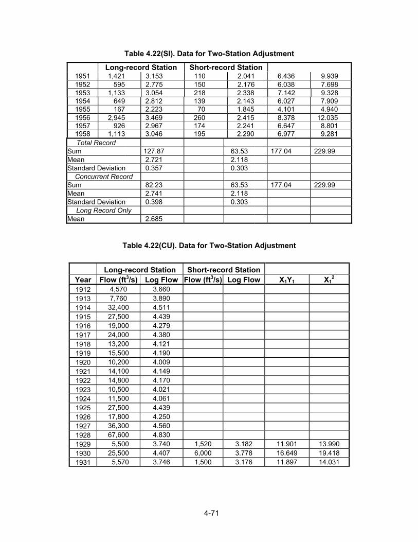
4-71

Table 4.22(SI). Data for Two-Station Adjustment

Long-record Station Short-record Station 1951 1,421 3.153 110 2.041 6.436 9.9391952 595 2.775 150 2.176 6.038 7.6981953 1,133 3.054 218 2.338 7.142 9.3281954 649 2.812 139 2.143 6.027 7.9091955 167 2.223 70 1.845 4.101 4.9401956 2,945 3.469 260 2.415 8.378 12.0351957 926 2.967 174 2.241 6.647 8.8011958 1,113 3.046 195 2.290 6.977 9.281Total Record

Sum 127.87 63.53 177.04 229.99 Mean 2.721 2.118 Standard Deviation 0.357 0.303

Concurrent Record Sum 82.23 63.53 177.04 229.99 Mean 2.741 2.118 Standard Deviation 0.398 0.303

Long Record Only Mean 2.685

Table 4.22(CU). Data for Two-Station Adjustment

Long-record Station Short-record Station

Year Flow (ft3/s)

Log Flow

Flow (ft3/s)

Log Flow X1Y1 X1

2 1912 4,570 3.660

1913 7,760 3.890

1914 32,400 4.511

1915 27,500 4.439

1916 19,000 4.279

1917 24,000 4.380

1918 13,200 4.121

1919 15,500 4.190

1920 10,200 4.009

1921 14,100 4.149

1922 14,800 4.170

1923 10,500 4.021

1924 11,500 4.061

1925 27,500 4.439

1926 17,800 4.250

1927 36,300 4.560

1928 67,600 4.830

1929 5,500 3.740 1,520 3.182 11.901 13.990 1930 25,500 4.407 6,000 3.778 16.649 19.418 1931 5,570 3.746 1,500 3.176 11.897 14.031

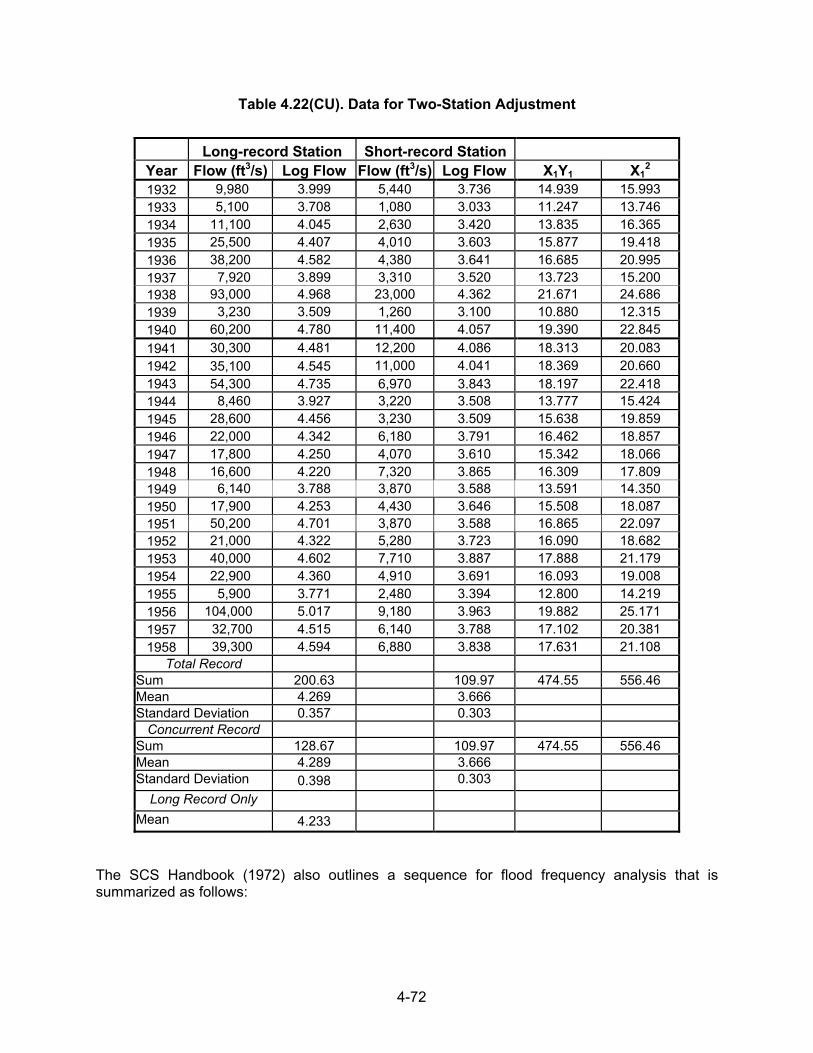
4-72

Table 4.22(CU). Data for Two-Station Adjustment

Long-record Station Short-record Station

Year Flow (ft3/s)

Log Flow

Flow (ft3/s)

Log Flow X1Y1 X1

2 1932 9,980 3.999 5,440 3.736 14.939 15.993 1933 5,100 3.708 1,080 3.033 11.247 13.746 1934 11,100 4.045 2,630 3.420 13.835 16.365 1935 25,500 4.407 4,010 3.603 15.877 19.418 1936 38,200 4.582 4,380 3.641 16.685 20.995 1937 7,920 3.899 3,310 3.520 13.723 15.200 1938 93,000 4.968 23,000 4.362 21.671 24.686 1939 3,230 3.509 1,260 3.100 10.880 12.315 1940 60,200 4.780 11,400 4.057 19.390 22.845 1941 30,300 4.481 12,200 4.086 18.313 20.083 1942 35,100 4.545 11,000 4.041 18.369 20.660 1943 54,300 4.735 6,970 3.843 18.197 22.418 1944 8,460 3.927 3,220 3.508 13.777 15.424 1945 28,600 4.456 3,230 3.509 15.638 19.859 1946 22,000 4.342 6,180 3.791 16.462 18.857 1947 17,800 4.250 4,070 3.610 15.342 18.066 1948 16,600 4.220 7,320 3.865 16.309 17.809 1949 6,140 3.788 3,870 3.588 13.591 14.350 1950 17,900 4.253 4,430 3.646 15.508 18.087 1951 50,200 4.701 3,870 3.588 16.865 22.097 1952 21,000 4.322 5,280 3.723 16.090 18.682 1953 40,000 4.602 7,710 3.887 17.888 21.179 1954 22,900 4.360 4,910 3.691 16.093 19.008 1955 5,900 3.771 2,480 3.394 12.800 14.219 1956 104,000 5.017 9,180 3.963 19.882 25.171 1957 32,700 4.515 6,140 3.788 17.102 20.381 1958 39,300 4.594 6,880 3.838 17.631 21.108

Total Record Sum 200.63 109.97 474.55 556.46 Mean 4.269 3.666 Standard Deviation 0.357 0.303

Concurrent Record Sum 128.67 109.97 474.55 556.46 Mean 4.289 3.666 Standard Deviation 0.398 0.303

Long Record Only Mean 4.233

The SCS Handbook (1972) also outlines a sequence for flood frequency analysis that is summarized as follows:

4-73

1. Obtain site information, the systematic station data, and historic information. These data should be examined for changes in watershed conditions, gage datum, flow regulation, etc. It is in this initial step that missing data should be estimated if indicated by the project.

2. Order the flood data, determine the plotting position, and plot the data on selected

probability graph paper (usually log-probability). Examine the data trend to select the standard distribution that best describes the population from which the sample is taken. Use a mixed-population analysis if indicated by the data trend and the watershed information.

3. Compute the sample statistics and the frequency curve for the selected distribution. Plot the

frequency curve with the station data to determine how well the flood data are distributed according to the selected distribution.

4. Check for high and low outliers. Adjust for historic data, retain or eliminate outliers, and

recompute the frequency curve. 5. Adjust data for missing low flows and zero flows and recompute the frequency curve. 6. Check the resulting frequency curve for reliability.

4.3.8 Other Methods for Estimating Flood Frequency Curves The techniques of fitting an annual series of flood data by the standard frequency distributions described above are all samples of the application of the method of moments. Population moments are estimated from the sample moments with the mean taken as the first moment about the origin, the variance as the second moment about the mean, and the skew as the third moment about the mean. Three other recognized methods are used to determine frequency curves. They include the method of maximum likelihood, the L-moments or probability weighted moments, and a graphical method. The method of maximum likelihood is a statistical technique based on the principle that the values of the statistical parameters of the sample are maximized so that the probability of obtaining an observed event is as high as possible. The method is somewhat more efficient for highly skewed distributions, if in fact efficient estimates of the statistical parameters exist. On the other hand, the method is very complicated to use and its practical use in highway design is not justified in view of the wide acceptance and use of the method of moments for fitting data with standard distributions. The method of maximum likelihood is described in detail by Kite (1988) and appropriate tables are presented from which the standard distributions can be determined.

Graphical methods involve simply fitting a curve to the sample data by eye. Typically the data are transformed by plotting on probability or log-probability graph paper so that a straight line can be obtained. This procedure is the least efficient, but, as noted in Sanders (1980), some improvement is obtained by ensuring that the maximum positive and negative deviations from the selected line are equal and that the maximum deviations are made as small as possible. This is, however, an expedient method by which highway designers can obtain a frequency distribution estimate.

4.3.9 Low-flow Frequency Analysis While instantaneous maximum discharges are used for flood frequency analyses, hydrologists are frequently interested in low flows. Low-flow frequency analyses are needed as part of water-

4-74

quality studies and the design of culverts where fish passage is a design criterion. For low-flow frequency analyses, it is common to specify both a return period and a flow duration. For example, a low-flow frequency curve may be computed for a 7-day duration. In this case, the 10-year event would be referred to as the 7-day, 10-year low flow. A data record to make a low-flow frequency analysis is compiled by identifying the lowest mean flow rate in each year of record for the given duration. For example, if the 21-day low-flow frequency curve is needed, the record for each year is analyzed to find the 21-day period in which the mean flow is the lowest. A moving-average smoothing analysis with a 21-day smoothing interval could be used to identify this flow. For a record of N years, such an analysis will yield N low flows for the needed duration. The computational procedure for making a low-flow frequency analysis is very similar to that for a flood frequency analysis. It is first necessary to specify the probability distribution. The log-normal distribution is most commonly used, although another distribution could be used. To make a log-normal analysis, a logarithmic transform of each of the N low flows is made. The mean and standard deviation of the logarithms are computed. Up to this point, the analysis is the same as for an analysis of peak flood flows. However, for a low-flow analysis, the governing equation is as follows:

LL Sz Y = Y log − (4.72) where, YL, SL = logarithmic mean and standard deviation, respectively z = standard normal deviate. Note that Equation 4.73 includes a minus sign rather than the plus sign of Equation 4.27. Thus, the low-flow frequency curve will have a negative slope rather than the positive slope that is typical of peak-flow frequency curves. Also, computed low flows for the less frequent events (e.g., the 100-year low flow) will be less than the mean. For example, if the logarithmic statistics for a 7-day low-flow record are QL = 1.1 and SL = 0.2, the 7-day, 50-year low flow is:

)sft170(sm4.9 = Q 0.6892=(0.2)2.054-1.1= Y log33

To plot the data points so they can be compared with the computed population curve, the low flows are ranked from smallest to largest (not largest to smallest as with a peak-flow analysis). The smallest flow is given a rank of 1 and the largest flow is given a rank of N. A plotting position formula (Equation 4.21) can then be selected to compute the probabilities. Each magnitude is plotted against the corresponding probability. The probability is plotted on the upper horizontal axis and is interpreted as the probability that the flow in any one time period will be less than the value on the frequency curve. For the calculation provided above, there is a 2 percent chance that the 7-day mean flow will be less than 4.9 m3/s (170 ft3/s) in any one year.

4-75

4.4 INDEX ADJUSTMENT OF FLOOD RECORDS The flood frequency methods of this chapter assume that the flood record is a series of events from the same population. In statistical terms, the events should be independent and identically distributed. In hydrologic terms, the events should be the result of the same meteorological and runoff processes. The year-to-year variation should only be due to the natural variation such as that of the volumes and durations of rainfall events. Watershed changes, such as deforestation and urbanization, change the runoff processes that control the watershed response to rainfall. In statistical terms, the events are no longer identically distributed because the population changes with changes in land use. Afforestation might decrease the mean flow. Urbanization would probably increase the mean flow but decrease the variation of the peak discharges. If the watershed change takes place over an extended period, each event during the period of change is from a different population. Thus, magnitudes and exceedence probabilities obtained from the flood record could not represent future events. Before such a record is used for a frequency analysis, the measured events should be adjusted to reflect homogeneous watershed conditions. One method of adjusting a flood record is referred to as the index-adjustment method (which should not be confused with the index-flood method of Chapter 5). Flood records can be adjusted using an index method, which is a class of methods that uses an index variable, such as the percentage of imperviousness or the fraction of a channel reach that has undergone channelization, to adjust the flood peaks. Index methods require values of the index variable for each year of the record and a model that relates the change in peak discharge, the index variable, and the exceedence probability. In addition to urbanization, index methods could be calibrated to adjust for the effects of deforestation, surface mining activity, agricultural management practices, or climate change.

4.4.1 Index Adjustment Method for Urbanization Since urbanization is a common cause of nonhomogeneity in flood records, it will be used to illustrate index adjustment of floods. The literature does not identify a single method that is considered to be the best method for adjusting an annual flood series when only the time record of urbanization is available. Furthermore, urbanization may be defined by a number of parameters, which include, but are not limited to: percent imperviousness, percent urbanized land cover (residential, commercial, and industrial), and population density. Each method depends on the data used to calibrate the prediction process, and the data used to calibrate the methods are usually very sparse. However, the sensitivities of measured peak discharges suggest that a 1 percent increase in percent imperviousness causes an increase in peak discharge of about 1 to 2.5 percent for the 100-year and the 2-year events, respectively (McCuen, 1989). Based on the general trends of results published in available urban flood-frequency studies, McCuen (1989) developed a method of adjusting a flood record for the effects of urbanization. Urbanization refers to the introduction of impervious surfaces or improvements of the hydraulic characteristics of the channels or principal flow paths. Figure 4.16 shows the peak adjustment factor as a function of the exceedence probability for percentages of imperviousness up to 60 percent. The greatest effect is for the more frequent events and the highest percentage of imperviousness. For this discussion, percent imperviousness is used as the measure of urbanization.

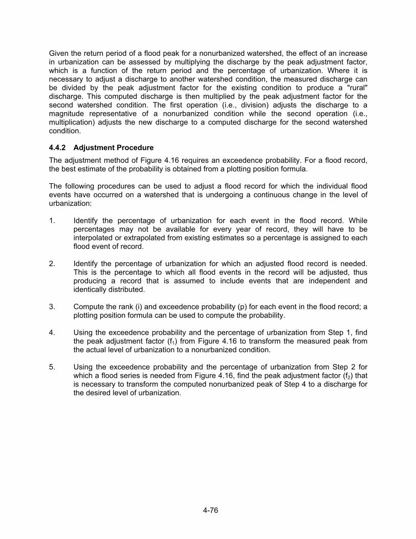
4-76

Given the return period of a flood peak for a nonurbanized watershed, the effect of an increase in urbanization can be assessed by multiplying the discharge by the peak adjustment factor, which is a function of the return period and the percentage of urbanization. Where it is necessary to adjust a discharge to another watershed condition, the measured discharge can be divided by the peak adjustment factor for the existing condition to produce a "rural" discharge. This computed discharge is then multiplied by the peak adjustment factor for the second watershed condition. The first operation (i.e., division) adjusts the discharge to a magnitude representative of a nonurbanized condition while the second operation (i.e., multiplication) adjusts the new discharge to a computed discharge for the second watershed condition.

4.4.2 Adjustment Procedure The adjustment method of Figure 4.16 requires an exceedence probability. For a flood record, the best estimate of the probability is obtained from a plotting position formula. The following procedures can be used to adjust a flood record for which the individual flood events have occurred on a watershed that is undergoing a continuous change in the level of urbanization: 1. Identify the percentage of urbanization for each event in the flood record. While

percentages may not be available for every year of record, they will have to be interpolated or extrapolated from existing estimates so a percentage is assigned to each flood event of record.

2. Identify the percentage of urbanization for which an adjusted flood record is needed.

This is the percentage to which all flood events in the record will be adjusted, thus producing a record that is assumed to include events that are independent and identically distributed.

3. Compute the rank (i) and exceedence probability (p) for each event in the flood record; a

plotting position formula can be used to compute the probability. 4. Using the exceedence probability and the percentage of urbanization from Step 1, find

the peak adjustment factor (f1) from Figure 4.16 to transform the measured peak from the actual level of urbanization to a nonurbanized condition.

5. Using the exceedence probability and the percentage of urbanization from Step 2 for

which a flood series is needed from Figure 4.16, find the peak adjustment factor (f2) that is necessary to transform the computed nonurbanized peak of Step 4 to a discharge for the desired level of urbanization.

4-77

6. Compute the adjusted discharge (Qa) by:

Qff = Q

1

2a (4.73)

in which Q is the measured discharge.

7. Repeat Steps 4, 5, and 6 for each event in the flood record and rank the adjusted series. 8. If the ranks of the events in the adjusted series differ from the ranks of the previous

series, which would be the measured events after one iteration of Steps 3 to 7, then the iteration process should be repeated until the ranks do not change.

3.0

2.5

2.0

1.5

3.0

2.5

2.0

1.5

99.99 99.9 99 98 95 90 80 70 50 30 0.05 0.010.215 21020

99.9999.999989590807050300.050.01 0.2 1 52 10 20

Exceedence probability (%)

0%

Peak

adj

ustm

ent

10%

20%

30%

40%

50%Imperviousness = 60%

Non-exceedence probability (%)

Figure 4.16. Peak adjustment factors for correcting a flood discharge magnitude for the change in imperviousness (from McCuen, 1989)

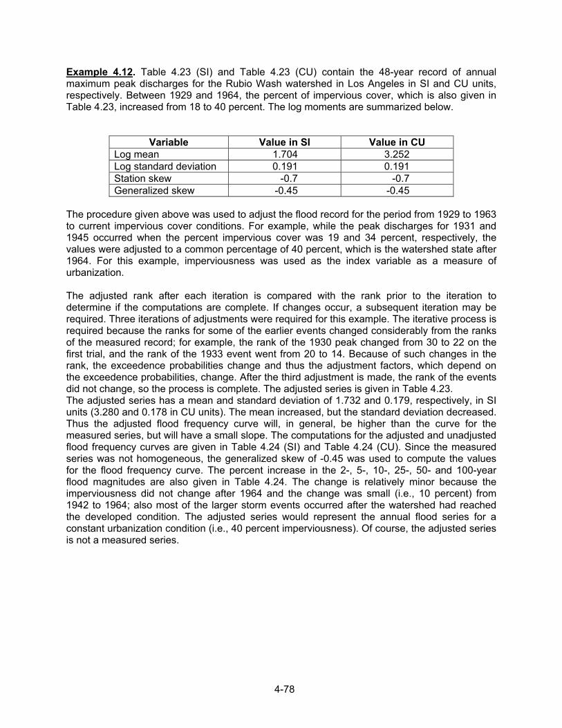
4-78

Example 4.12. Table 4.23 (SI) and Table 4.23 (CU) contain the 48-year record of annual maximum peak discharges for the Rubio Wash watershed in Los Angeles in SI and CU units, respectively. Between 1929 and 1964, the percent of impervious cover, which is also given in Table 4.23, increased from 18 to 40 percent. The log moments are summarized below.

Variable Value in SI Value in CU Log mean 1.704 3.252 Log standard deviation 0.191 0.191 Station skew -0.7 -0.7 Generalized skew -0.45 -0.45

The procedure given above was used to adjust the flood record for the period from 1929 to 1963 to current impervious cover conditions. For example, while the peak discharges for 1931 and 1945 occurred when the percent impervious cover was 19 and 34 percent, respectively, the values were adjusted to a common percentage of 40 percent, which is the watershed state after 1964. For this example, imperviousness was used as the index variable as a measure of urbanization. The adjusted rank after each iteration is compared with the rank prior to the iteration to determine if the computations are complete. If changes occur, a subsequent iteration may be required. Three iterations of adjustments were required for this example. The iterative process is required because the ranks for some of the earlier events changed considerably from the ranks of the measured record; for example, the rank of the 1930 peak changed from 30 to 22 on the first trial, and the rank of the 1933 event went from 20 to 14. Because of such changes in the rank, the exceedence probabilities change and thus the adjustment factors, which depend on the exceedence probabilities, change. After the third adjustment is made, the rank of the events did not change, so the process is complete. The adjusted series is given in Table 4.23. The adjusted series has a mean and standard deviation of 1.732 and 0.179, respectively, in SI units (3.280 and 0.178 in CU units). The mean increased, but the standard deviation decreased. Thus the adjusted flood frequency curve will, in general, be higher than the curve for the measured series, but will have a small slope. The computations for the adjusted and unadjusted flood frequency curves are given in Table 4.24 (SI) and Table 4.24 (CU). Since the measured series was not homogeneous, the generalized skew of -0.45 was used to compute the values for the flood frequency curve. The percent increase in the 2-, 5-, 10-, 25-, 50- and 100-year flood magnitudes are also given in Table 4.24. The change is relatively minor because the imperviousness did not change after 1964 and the change was small (i.e., 10 percent) from 1942 to 1964; also most of the larger storm events occurred after the watershed had reached the developed condition. The adjusted series would represent the annual flood series for a constant urbanization condition (i.e., 40 percent imperviousness). Of course, the adjusted series is not a measured series.

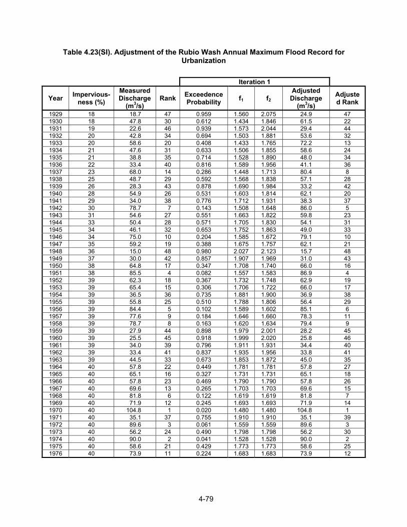
4-79

Table 4.23(SI). Adjustment of the Rubio Wash Annual Maximum Flood Record for Urbanization

Iteration 1

Year Impervious-ness (%)

Measured Discharge

(m3/s) Rank Exceedence

Probability f1 f2

Adjusted Discharge

(m3/s) Adjusted Rank

1929 18 18.7 47 0.959 1.560 2.075 24.9 47 1930 18 47.8 30 0.612 1.434 1.846 61.5 22 1931 19 22.6 46 0.939 1.573 2.044 29.4 44 1932 20 42.8 34 0.694 1.503 1.881 53.6 32 1933 20 58.6 20 0.408 1.433 1.765 72.2 13 1934 21 47.6 31 0.633 1.506 1.855 58.6 24 1935 21 38.8 35 0.714 1.528 1.890 48.0 34 1936 22 33.4 40 0.816 1.589 1.956 41.1 36 1937 23 68.0 14 0.286 1.448 1.713 80.4 8 1938 25 48.7 29 0.592 1.568 1.838 57.1 28 1939 26 28.3 43 0.878 1.690 1.984 33.2 42 1940 28 54.9 26 0.531 1.603 1.814 62.1 20 1941 29 34.0 38 0.776 1.712 1.931 38.3 37 1942 30 78.7 7 0.143 1.508 1.648 86.0 5 1943 31 54.6 27 0.551 1.663 1.822 59.8 23 1944 33 50.4 28 0.571 1.705 1.830 54.1 31 1945 34 46.1 32 0.653 1.752 1.863 49.0 33 1946 34 75.0 10 0.204 1.585 1.672 79.1 10 1947 35 59.2 19 0.388 1.675 1.757 62.1 21 1948 36 15.0 48 0.980 2.027 2.123 15.7 48 1949 37 30.0 42 0.857 1.907 1.969 31.0 43 1950 38 64.8 17 0.347 1.708 1.740 66.0 16 1951 38 85.5 4 0.082 1.557 1.583 86.9 4 1952 39 62.3 18 0.367 1.732 1.748 62.9 19 1953 39 65.4 15 0.306 1.706 1.722 66.0 17 1954 39 36.5 36 0.735 1.881 1.900 36.9 38 1955 39 55.8 25 0.510 1.788 1.806 56.4 29 1956 39 84.4 5 0.102 1.589 1.602 85.1 6 1957 39 77.6 9 0.184 1.646 1.660 78.3 11 1958 39 78.7 8 0.163 1.620 1.634 79.4 9 1959 39 27.9 44 0.898 1.979 2.001 28.2 45 1960 39 25.5 45 0.918 1.999 2.020 25.8 46 1961 39 34.0 39 0.796 1.911 1.931 34.4 40 1962 39 33.4 41 0.837 1.935 1.956 33.8 41 1963 39 44.5 33 0.673 1.853 1.872 45.0 35 1964 40 57.8 22 0.449 1.781 1.781 57.8 27 1965 40 65.1 16 0.327 1.731 1.731 65.1 18 1966 40 57.8 23 0.469 1.790 1.790 57.8 26 1967 40 69.6 13 0.265 1.703 1.703 69.6 15 1968 40 81.8 6 0.122 1.619 1.619 81.8 7 1969 40 71.9 12 0.245 1.693 1.693 71.9 14 1970 40 104.8 1 0.020 1.480 1.480 104.8 1 1971 40 35.1 37 0.755 1.910 1.910 35.1 39 1972 40 89.6 3 0.061 1.559 1.559 89.6 3 1973 40 56.2 24 0.490 1.798 1.798 56.2 30 1974 40 90.0 2 0.041 1.528 1.528 90.0 2 1975 40 58.6 21 0.429 1.773 1.773 58.6 25 1976 40 73.9 11 0.224 1.683 1.683 73.9 12

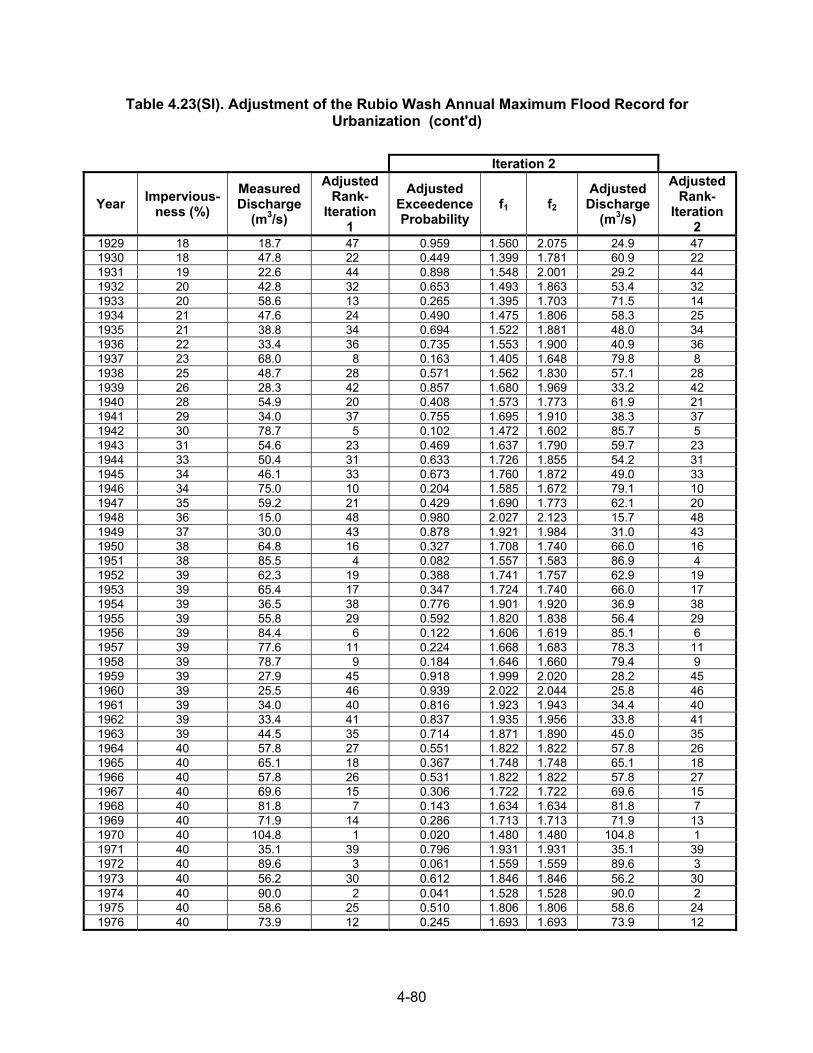
4-80

Table 4.23(SI). Adjustment of the Rubio Wash Annual Maximum Flood Record for Urbanization (cont'd)

Iteration 2

Year Impervious-ness (%)

Measured Discharge

(m3/s)

Adjusted Rank-

Iteration 1

Adjusted Exceedence Probability

f1 f2

Adjusted Discharge

(m3/s)

Adjusted Rank-

Iteration 2

1929 18 18.7 47 0.959 1.560 2.075 24.9 47 1930 18 47.8 22 0.449 1.399 1.781 60.9 22 1931 19 22.6 44 0.898 1.548 2.001 29.2 44 1932 20 42.8 32 0.653 1.493 1.863 53.4 32 1933 20 58.6 13 0.265 1.395 1.703 71.5 14 1934 21 47.6 24 0.490 1.475 1.806 58.3 25 1935 21 38.8 34 0.694 1.522 1.881 48.0 34 1936 22 33.4 36 0.735 1.553 1.900 40.9 36 1937 23 68.0 8 0.163 1.405 1.648 79.8 8 1938 25 48.7 28 0.571 1.562 1.830 57.1 28 1939 26 28.3 42 0.857 1.680 1.969 33.2 42 1940 28 54.9 20 0.408 1.573 1.773 61.9 21 1941 29 34.0 37 0.755 1.695 1.910 38.3 37 1942 30 78.7 5 0.102 1.472 1.602 85.7 5 1943 31 54.6 23 0.469 1.637 1.790 59.7 23 1944 33 50.4 31 0.633 1.726 1.855 54.2 31 1945 34 46.1 33 0.673 1.760 1.872 49.0 33 1946 34 75.0 10 0.204 1.585 1.672 79.1 10 1947 35 59.2 21 0.429 1.690 1.773 62.1 20 1948 36 15.0 48 0.980 2.027 2.123 15.7 48 1949 37 30.0 43 0.878 1.921 1.984 31.0 43 1950 38 64.8 16 0.327 1.708 1.740 66.0 16 1951 38 85.5 4 0.082 1.557 1.583 86.9 4 1952 39 62.3 19 0.388 1.741 1.757 62.9 19 1953 39 65.4 17 0.347 1.724 1.740 66.0 17 1954 39 36.5 38 0.776 1.901 1.920 36.9 38 1955 39 55.8 29 0.592 1.820 1.838 56.4 29 1956 39 84.4 6 0.122 1.606 1.619 85.1 6 1957 39 77.6 11 0.224 1.668 1.683 78.3 11 1958 39 78.7 9 0.184 1.646 1.660 79.4 9 1959 39 27.9 45 0.918 1.999 2.020 28.2 45 1960 39 25.5 46 0.939 2.022 2.044 25.8 46 1961 39 34.0 40 0.816 1.923 1.943 34.4 40 1962 39 33.4 41 0.837 1.935 1.956 33.8 41 1963 39 44.5 35 0.714 1.871 1.890 45.0 35 1964 40 57.8 27 0.551 1.822 1.822 57.8 26 1965 40 65.1 18 0.367 1.748 1.748 65.1 18 1966 40 57.8 26 0.531 1.822 1.822 57.8 27 1967 40 69.6 15 0.306 1.722 1.722 69.6 15 1968 40 81.8 7 0.143 1.634 1.634 81.8 7 1969 40 71.9 14 0.286 1.713 1.713 71.9 13 1970 40 104.8 1 0.020 1.480 1.480 104.8 1 1971 40 35.1 39 0.796 1.931 1.931 35.1 39 1972 40 89.6 3 0.061 1.559 1.559 89.6 3 1973 40 56.2 30 0.612 1.846 1.846 56.2 30 1974 40 90.0 2 0.041 1.528 1.528 90.0 2 1975 40 58.6 25 0.510 1.806 1.806 58.6 24 1976 40 73.9 12 0.245 1.693 1.693 73.9 12

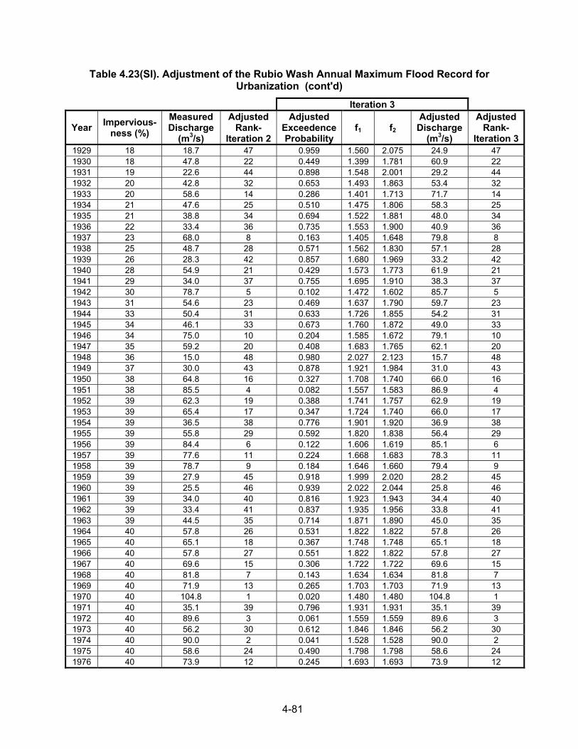
4-81

Table 4.23(SI). Adjustment of the Rubio Wash Annual Maximum Flood Record for Urbanization (cont'd)

Iteration 3

Year Impervious-ness (%)

Measured Discharge

(m3/s)

Adjusted Rank-

Iteration 2

Adjusted Exceedence Probability

f1 f2

Adjusted Discharge

(m3/s)

Adjusted Rank-

Iteration 31929 18 18.7 47 0.959 1.560 2.075 24.9 47 1930 18 47.8 22 0.449 1.399 1.781 60.9 22 1931 19 22.6 44 0.898 1.548 2.001 29.2 44 1932 20 42.8 32 0.653 1.493 1.863 53.4 32 1933 20 58.6 14 0.286 1.401 1.713 71.7 14 1934 21 47.6 25 0.510 1.475 1.806 58.3 25 1935 21 38.8 34 0.694 1.522 1.881 48.0 34 1936 22 33.4 36 0.735 1.553 1.900 40.9 36 1937 23 68.0 8 0.163 1.405 1.648 79.8 8 1938 25 48.7 28 0.571 1.562 1.830 57.1 28 1939 26 28.3 42 0.857 1.680 1.969 33.2 42 1940 28 54.9 21 0.429 1.573 1.773 61.9 21 1941 29 34.0 37 0.755 1.695 1.910 38.3 37 1942 30 78.7 5 0.102 1.472 1.602 85.7 5 1943 31 54.6 23 0.469 1.637 1.790 59.7 23 1944 33 50.4 31 0.633 1.726 1.855 54.2 31 1945 34 46.1 33 0.673 1.760 1.872 49.0 33 1946 34 75.0 10 0.204 1.585 1.672 79.1 10 1947 35 59.2 20 0.408 1.683 1.765 62.1 20 1948 36 15.0 48 0.980 2.027 2.123 15.7 48 1949 37 30.0 43 0.878 1.921 1.984 31.0 43 1950 38 64.8 16 0.327 1.708 1.740 66.0 16 1951 38 85.5 4 0.082 1.557 1.583 86.9 4 1952 39 62.3 19 0.388 1.741 1.757 62.9 19 1953 39 65.4 17 0.347 1.724 1.740 66.0 17 1954 39 36.5 38 0.776 1.901 1.920 36.9 38 1955 39 55.8 29 0.592 1.820 1.838 56.4 29 1956 39 84.4 6 0.122 1.606 1.619 85.1 6 1957 39 77.6 11 0.224 1.668 1.683 78.3 11 1958 39 78.7 9 0.184 1.646 1.660 79.4 9 1959 39 27.9 45 0.918 1.999 2.020 28.2 45 1960 39 25.5 46 0.939 2.022 2.044 25.8 46 1961 39 34.0 40 0.816 1.923 1.943 34.4 40 1962 39 33.4 41 0.837 1.935 1.956 33.8 41 1963 39 44.5 35 0.714 1.871 1.890 45.0 35 1964 40 57.8 26 0.531 1.822 1.822 57.8 26 1965 40 65.1 18 0.367 1.748 1.748 65.1 18 1966 40 57.8 27 0.551 1.822 1.822 57.8 27 1967 40 69.6 15 0.306 1.722 1.722 69.6 15 1968 40 81.8 7 0.143 1.634 1.634 81.8 7 1969 40 71.9 13 0.265 1.703 1.703 71.9 13 1970 40 104.8 1 0.020 1.480 1.480 104.8 1 1971 40 35.1 39 0.796 1.931 1.931 35.1 39 1972 40 89.6 3 0.061 1.559 1.559 89.6 3 1973 40 56.2 30 0.612 1.846 1.846 56.2 30 1974 40 90.0 2 0.041 1.528 1.528 90.0 2 1975 40 58.6 24 0.490 1.798 1.798 58.6 24 1976 40 73.9 12 0.245 1.693 1.693 73.9 12

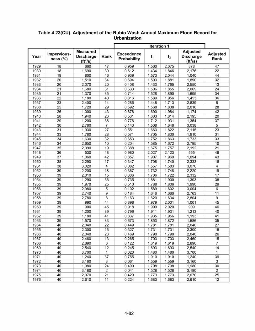
4-82

Table 4.23(CU). Adjustment of the Rubio Wash Annual Maximum Flood Record for Urbanization

Iteration 1

Year Impervious-ness (%)

Measured Discharge

(ft3/s) Rank Exceedence

Probability f1 f2

Adjusted Discharge

(ft3/s) Adjusted

Rank 1929 18 660 47 0.959 1.560 2.075 878 47 1930 18 1,690 30 0.612 1.434 1.846 2,176 22 1931 19 800 46 0.939 1.573 2.044 1,040 44 1932 20 1,510 34 0.694 1.503 1.881 1,890 32 1933 20 2,070 20 0.408 1.433 1.765 2,550 13 1934 21 1,680 31 0.633 1.506 1.855 2,069 24 1935 21 1,370 35 0.714 1.528 1.890 1,695 34 1936 22 1,180 40 0.816 1.589 1.956 1,453 36 1937 23 2,400 14 0.286 1.448 1.713 2,839 8 1938 25 1,720 29 0.592 1.568 1.838 2,016 28 1939 26 1,000 43 0.878 1.690 1.984 1,174 42 1940 28 1,940 26 0.531 1.603 1.814 2,195 20 1941 29 1,200 38 0.776 1.712 1.931 1,354 37 1942 30 2,780 7 0.143 1.508 1.648 3,038 5 1943 31 1,930 27 0.551 1.663 1.822 2,115 23 1944 33 1,780 28 0.571 1.705 1.830 1,910 31 1945 34 1,630 32 0.653 1.752 1.863 1,733 33 1946 34 2,650 10 0.204 1.585 1.672 2,795 10 1947 35 2,090 19 0.388 1.675 1.757 2,192 21 1948 36 530 48 0.980 2.027 2.123 555 48 1949 37 1,060 42 0.857 1.907 1.969 1,094 43 1950 38 2,290 17 0.347 1.708 1.740 2,333 16 1951 38 3,020 4 0.082 1.557 1.583 3,070 4 1952 39 2,200 18 0.367 1.732 1.748 2,220 19 1953 39 2,310 15 0.306 1.706 1.722 2,332 17 1954 39 1,290 36 0.735 1.881 1.900 1,303 38 1955 39 1,970 25 0.510 1.788 1.806 1,990 29 1956 39 2,980 5 0.102 1.589 1.602 3,004 6 1957 39 2,740 9 0.184 1.646 1.660 2,763 11 1958 39 2,780 8 0.163 1.620 1.634 2,804 9 1959 39 990 44 0.898 1.979 2.001 1,001 45 1960 39 900 45 0.918 1.999 2.020 909 46 1961 39 1,200 39 0.796 1.911 1.931 1,213 40 1962 39 1,180 41 0.837 1.935 1.956 1,193 41 1963 39 1,570 33 0.673 1.853 1.872 1,586 35 1964 40 2,040 22 0.449 1.781 1.781 2,040 27 1965 40 2,300 16 0.327 1.731 1.731 2,300 18 1966 40 2,040 23 0.469 1.790 1.790 2,040 26 1967 40 2,460 13 0.265 1.703 1.703 2,460 15 1968 40 2,890 6 0.122 1.619 1.619 2,890 7 1969 40 2,540 12 0.245 1.693 1.693 2,540 14 1970 40 3,700 1 0.020 1.480 1.480 3,700 1 1971 40 1,240 37 0.755 1.910 1.910 1,240 39 1972 40 3,160 3 0.061 1.559 1.559 3,160 3 1973 40 1,980 24 0.490 1.798 1.798 1,980 30 1974 40 3,180 2 0.041 1.528 1.528 3,180 2 1975 40 2,070 21 0.429 1.773 1.773 2,070 25 1976 40 2,610 11 0.224 1.683 1.683 2,610 12

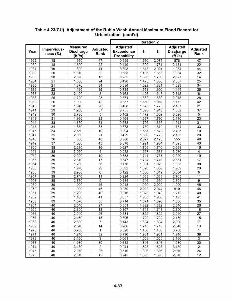
4-83

Table 4.23(CU). Adjustment of the Rubio Wash Annual Maximum Flood Record for Urbanization (cont'd)

Iteration 2

Year Impervious-ness (%)

Measured Discharge

(ft3/s) Adjusted

Rank Adjusted

Exceedence Probability

f1 f2 Adjusted

Discharge (ft3/s)

Adjusted Rank

1929 18 660 47 0.959 1.560 2.075 878 47 1930 18 1,690 22 0.449 1.399 1.781 2,151 22 1931 19 800 44 0.898 1.548 2.001 1,034 44 1932 20 1,510 32 0.653 1.493 1.863 1,884 32 1933 20 2,070 13 0.265 1.395 1.703 2,527 14 1934 21 1,680 24 0.490 1.475 1.806 2,057 25 1935 21 1,370 34 0.694 1.522 1.881 1,693 34 1936 22 1,180 36 0.735 1.553 1.900 1,444 36 1937 23 2,400 8 0.163 1.405 1.648 2,815 8 1938 25 1,720 28 0.571 1.562 1.830 2,015 28 1939 26 1,000 42 0.857 1.680 1.969 1,172 42 1940 28 1,940 20 0.408 1.573 1.773 2,187 21 1941 29 1,200 37 0.755 1.695 1.910 1,352 37 1942 30 2,780 5 0.102 1.472 1.602 3,026 5 1943 31 1,930 23 0.469 1.637 1.790 2,110 23 1944 33 1,780 31 0.633 1.726 1.855 1,913 31 1945 34 1,630 33 0.673 1.760 1.872 1,734 33 1946 34 2,650 10 0.204 1.585 1.672 2,795 10 1947 35 2,090 21 0.429 1.690 1.773 2,193 20 1948 36 530 48 0.980 2.027 2.123 555 48 1949 37 1,060 43 0.878 1.921 1.984 1,095 43 1950 38 2,290 16 0.327 1.708 1.740 2,333 16 1951 38 3,020 4 0.082 1.557 1.583 3,070 4 1952 39 2,200 19 0.388 1.741 1.757 2,220 19 1953 39 2,310 17 0.347 1.724 1.740 2,331 17 1954 39 1,290 38 0.776 1.901 1.920 1,303 38 1955 39 1,970 29 0.592 1.820 1.838 1,989 29 1956 39 2,980 6 0.122 1.606 1.619 3,004 6 1957 39 2,740 11 0.224 1.668 1.683 2,765 11 1958 39 2,780 9 0.184 1.646 1.660 2,804 9 1959 39 990 45 0.918 1.999 2.020 1,000 45 1960 39 900 46 0.939 2.022 2.044 910 46 1961 39 1,200 40 0.816 1.923 1.943 1,212 40 1962 39 1,180 41 0.837 1.935 1.956 1,193 41 1963 39 1,570 35 0.714 1.871 1.890 1,586 35 1964 40 2,040 27 0.551 1.822 1.822 2,040 26 1965 40 2,300 18 0.367 1.748 1.748 2,300 18 1966 40 2,040 26 0.531 1.822 1.822 2,040 27 1967 40 2,460 15 0.306 1.722 1.722 2,460 15 1968 40 2,890 7 0.143 1.634 1.634 2,890 7 1969 40 2,540 14 0.286 1.713 1.713 2,540 13 1970 40 3,700 1 0.020 1.480 1.480 3,700 1 1971 40 1,240 39 0.796 1.931 1.931 1,240 39 1972 40 3,160 3 0.061 1.559 1.559 3,160 3 1973 40 1,980 30 0.612 1.846 1.846 1,980 30 1974 40 3,180 2 0.041 1.528 1.528 3,180 2 1975 40 2,070 25 0.510 1.806 1.806 2,070 24 1976 40 2,610 12 0.245 1.693 1.693 2,610 12

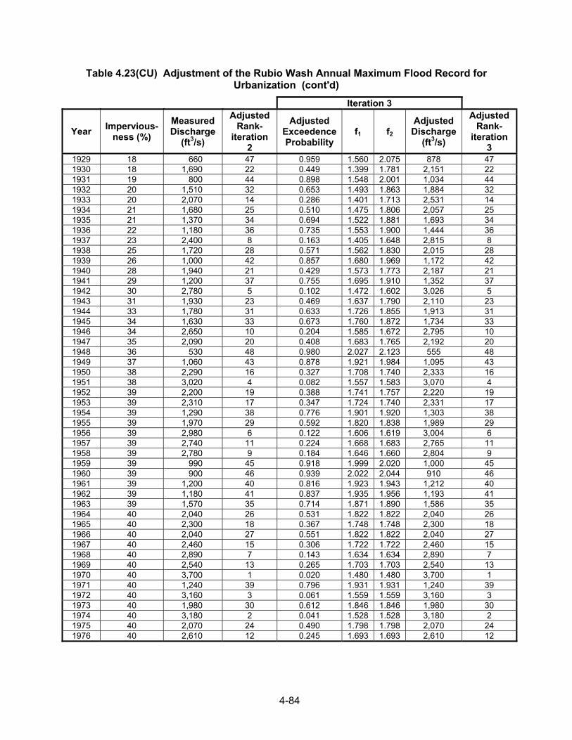
4-84

Table 4.23(CU) Adjustment of the Rubio Wash Annual Maximum Flood Record for Urbanization (cont'd)

Iteration 3

Year Impervious-ness (%)

Measured Discharge

(ft3/s)

Adjusted Rank-

iteration 2

Adjusted Exceedence Probability

f1 f2

Adjusted Discharge

(ft3/s)

Adjusted Rank-

iteration 3

1929 18 660 47 0.959 1.560 2.075 878 47 1930 18 1,690 22 0.449 1.399 1.781 2,151 22 1931 19 800 44 0.898 1.548 2.001 1,034 44 1932 20 1,510 32 0.653 1.493 1.863 1,884 32 1933 20 2,070 14 0.286 1.401 1.713 2,531 14 1934 21 1,680 25 0.510 1.475 1.806 2,057 25 1935 21 1,370 34 0.694 1.522 1.881 1,693 34 1936 22 1,180 36 0.735 1.553 1.900 1,444 36 1937 23 2,400 8 0.163 1.405 1.648 2,815 8 1938 25 1,720 28 0.571 1.562 1.830 2,015 28 1939 26 1,000 42 0.857 1.680 1.969 1,172 42 1940 28 1,940 21 0.429 1.573 1.773 2,187 21 1941 29 1,200 37 0.755 1.695 1.910 1,352 37 1942 30 2,780 5 0.102 1.472 1.602 3,026 5 1943 31 1,930 23 0.469 1.637 1.790 2,110 23 1944 33 1,780 31 0.633 1.726 1.855 1,913 31 1945 34 1,630 33 0.673 1.760 1.872 1,734 33 1946 34 2,650 10 0.204 1.585 1.672 2,795 10 1947 35 2,090 20 0.408 1.683 1.765 2,192 20 1948 36 530 48 0.980 2.027 2.123 555 48 1949 37 1,060 43 0.878 1.921 1.984 1,095 43 1950 38 2,290 16 0.327 1.708 1.740 2,333 16 1951 38 3,020 4 0.082 1.557 1.583 3,070 4 1952 39 2,200 19 0.388 1.741 1.757 2,220 19 1953 39 2,310 17 0.347 1.724 1.740 2,331 17 1954 39 1,290 38 0.776 1.901 1.920 1,303 38 1955 39 1,970 29 0.592 1.820 1.838 1,989 29 1956 39 2,980 6 0.122 1.606 1.619 3,004 6 1957 39 2,740 11 0.224 1.668 1.683 2,765 11 1958 39 2,780 9 0.184 1.646 1.660 2,804 9 1959 39 990 45 0.918 1.999 2.020 1,000 45 1960 39 900 46 0.939 2.022 2.044 910 46 1961 39 1,200 40 0.816 1.923 1.943 1,212 40 1962 39 1,180 41 0.837 1.935 1.956 1,193 41 1963 39 1,570 35 0.714 1.871 1.890 1,586 35 1964 40 2,040 26 0.531 1.822 1.822 2,040 26 1965 40 2,300 18 0.367 1.748 1.748 2,300 18 1966 40 2,040 27 0.551 1.822 1.822 2,040 27 1967 40 2,460 15 0.306 1.722 1.722 2,460 15 1968 40 2,890 7 0.143 1.634 1.634 2,890 7 1969 40 2,540 13 0.265 1.703 1.703 2,540 13 1970 40 3,700 1 0.020 1.480 1.480 3,700 1 1971 40 1,240 39 0.796 1.931 1.931 1,240 39 1972 40 3,160 3 0.061 1.559 1.559 3,160 3 1973 40 1,980 30 0.612 1.846 1.846 1,980 30 1974 40 3,180 2 0.041 1.528 1.528 3,180 2 1975 40 2,070 24 0.490 1.798 1.798 2,070 24 1976 40 2,610 12 0.245 1.693 1.693 2,610 12

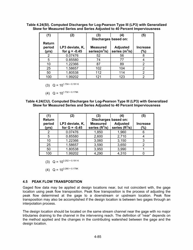
4-85

Table 4.24(SI). Computed Discharges for Log-Pearson Type III (LP3) with Generalized Skew for Measured Series and Series Adjusted to 40 Percent Imperviousness

(1) (2) (3) (4) (5) Discharges based on:

Return period (yrs)

LP3 deviate, K, for g = -0.45

Measured series(m3/s)

Adjusted series (m3/s)

Increase (%)

2 0.07476 52 56 8 5 0.85580 74 77 4

10 1.22366 87 89 2 25 1.58657 102 104 2 50 1.80538 112 114 2

100 1.99202 121 123 2 (3) Q = 101.704 + 0.191 K (4) Q = 101.732 + 0.179K

Table 4.24(CU). Computed Discharges for Log-Pearson Type III (LP3) with Generalized

Skew for Measured Series and Series Adjusted to 40 Percent Imperviousness

(1) (2) (3) (4) (5) Discharges based on: Return

period (yrs)

LP3 deviate, K, for G = -0.45

Measured series (ft3/s)

Adjusted series (ft3/s)

Increase (%)

2 0.07476 1,850 1,960 6 5 0.85580 2,600 2,710 4

10 1.22366 3,060 3,150 3 25 1.58657 3,590 3,650 2 50 1.80538 3,950 3,990 1

100 1.99202 4,290 4,310 0 (3) Q = 103.252 + 0.191 K (4) Q = 103.280 + 0.179K

4.5 PEAK FLOW TRANSPOSITION Gaged flow data may be applied at design locations near, but not coincident with, the gage location using peak flow transposition. Peak flow transposition is the process of adjusting the peak flow determined at the gage to a downstream or upstream location. Peak flow transposition may also be accomplished if the design location is between two gages through an interpolation process. The design location should be located on the same stream channel near the gage with no major tributaries draining to the channel in the intervening reach. The definition of “near” depends on the method applied and the changes in the contributing watershed between the gage and the design location.

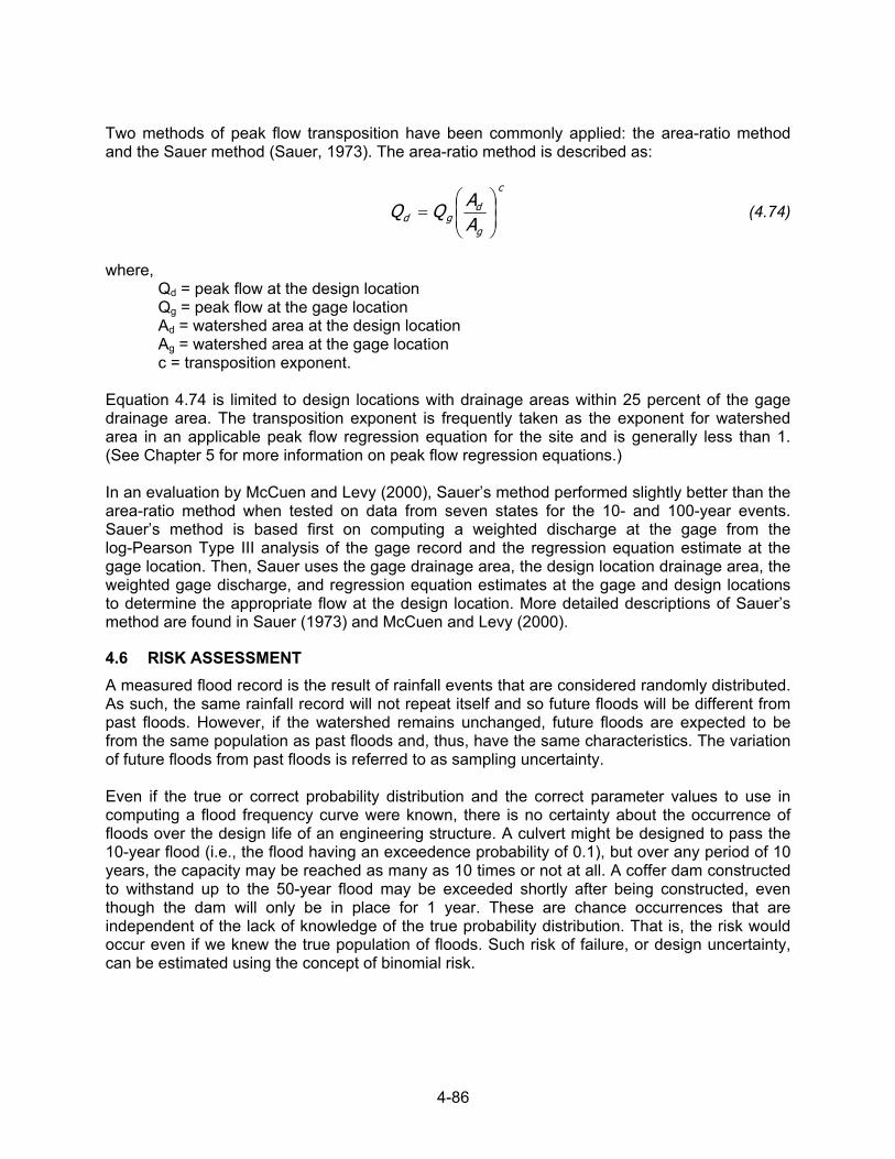
4-86

Two methods of peak flow transposition have been commonly applied: the area-ratio method and the Sauer method (Sauer, 1973). The area-ratio method is described as:

c

g

dgd A

AQQ

= (4.74)

where, Qd = peak flow at the design location Qg = peak flow at the gage location Ad = watershed area at the design location Ag = watershed area at the gage location c = transposition exponent. Equation 4.74 is limited to design locations with drainage areas within 25 percent of the gage drainage area. The transposition exponent is frequently taken as the exponent for watershed area in an applicable peak flow regression equation for the site and is generally less than 1. (See Chapter 5 for more information on peak flow regression equations.) In an evaluation by McCuen and Levy (2000), Sauer’s method performed slightly better than the area-ratio method when tested on data from seven states for the 10- and 100-year events. Sauer’s method is based first on computing a weighted discharge at the gage from the log-Pearson Type III analysis of the gage record and the regression equation estimate at the gage location. Then, Sauer uses the gage drainage area, the design location drainage area, the weighted gage discharge, and regression equation estimates at the gage and design locations to determine the appropriate flow at the design location. More detailed descriptions of Sauer’s method are found in Sauer (1973) and McCuen and Levy (2000).

4.6 RISK ASSESSMENT A measured flood record is the result of rainfall events that are considered randomly distributed. As such, the same rainfall record will not repeat itself and so future floods will be different from past floods. However, if the watershed remains unchanged, future floods are expected to be from the same population as past floods and, thus, have the same characteristics. The variation of future floods from past floods is referred to as sampling uncertainty. Even if the true or correct probability distribution and the correct parameter values to use in computing a flood frequency curve were known, there is no certainty about the occurrence of floods over the design life of an engineering structure. A culvert might be designed to pass the 10-year flood (i.e., the flood having an exceedence probability of 0.1), but over any period of 10 years, the capacity may be reached as many as 10 times or not at all. A coffer dam constructed to withstand up to the 50-year flood may be exceeded shortly after being constructed, even though the dam will only be in place for 1 year. These are chance occurrences that are independent of the lack of knowledge of the true probability distribution. That is, the risk would occur even if we knew the true population of floods. Such risk of failure, or design uncertainty, can be estimated using the concept of binomial risk.

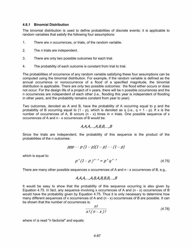
4-87

4.6.1 Binomial Distribution The binomial distribution is used to define probabilities of discrete events; it is applicable to random variables that satisfy the following four assumptions: 1. There are n occurrences, or trials, of the random variable. 2. The n trials are independent. 3. There are only two possible outcomes for each trial. 4. The probability of each outcome is constant from trial to trial. The probabilities of occurrence of any random variable satisfying these four assumptions can be computed using the binomial distribution. For example, if the random variable is defined as the annual occurrence or nonoccurrence of a flood of a specified magnitude, the binomial distribution is applicable. There are only two possible outcomes: the flood either occurs or does not occur. For the design life of a project of n years, there will be n possible occurrences and the n occurrences are independent of each other (i.e., flooding this year is independent of flooding in other years, and the probability remains constant from year to year). Two outcomes, denoted as A and B, have the probability of A occurring equal to p and the probability of B occurring equal to (1 - p), which is denoted as q (i.e., q = 1 - p). If x is the number of occurrences of A, B occurs (n - x) times in n trials. One possible sequence of x occurrences of A and n - x occurrences of B would be:

A,A,A,…,A,B,B,…,B Since the trials are independent, the probability of this sequence is the product of the probabilities of the n outcomes:

p)(1 p)p)(1 (1 p ppp −⋅⋅⋅−−⋅⋅⋅ which is equal to:

qp = ) p (1p x nxx nx −−− (4.75)

There are many other possible sequences x occurrences of A and n - x occurrences of B, e.g.,

A,A,A,…,A,B,A,B,B,B,…,B It would be easy to show that the probability of this sequence occurring is also given by Equation 4.75. In fact, any sequence involving x occurrences of A and (n - x) occurrences of B would have the probability given by Equation 4.75. Thus it is only necessary to determine how many different sequences of x occurrences of A and (n - x) occurrences of B are possible. It can be shown that the number of occurrences is:

!)xn(!x

!n−

(4.76)

where n! is read "n factorial" and equals:

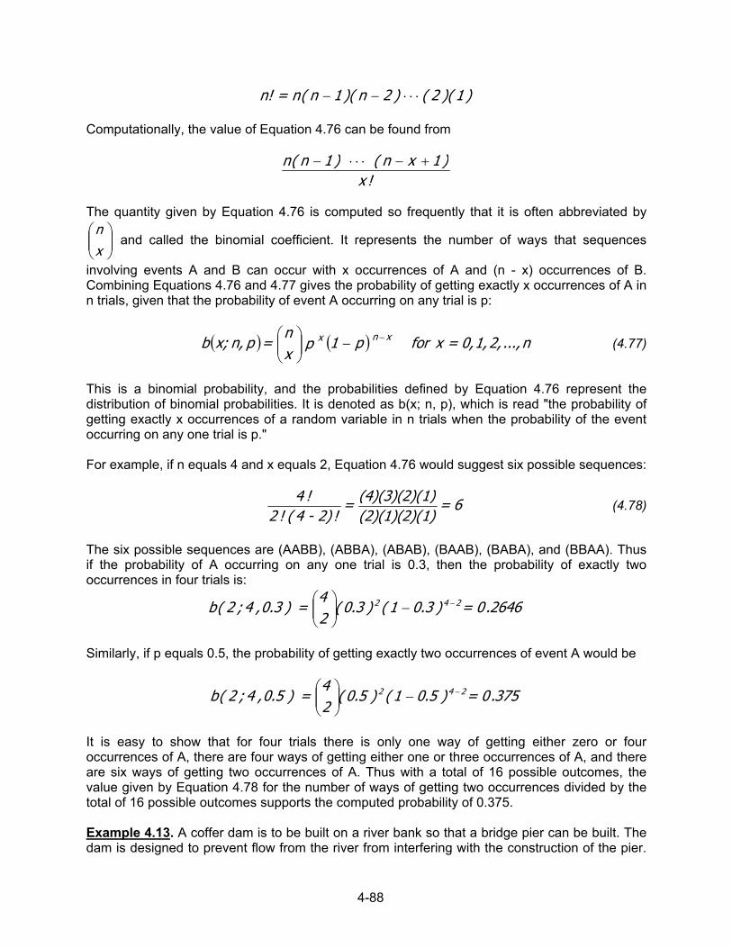
4-88

)1)(2()2n)(1n(n! = n ⋅⋅⋅−− Computationally, the value of Equation 4.76 can be found from

!x)1xn()1n(n +−⋅⋅⋅−

The quantity given by Equation 4.76 is computed so frequently that it is often abbreviated by

xn

and called the binomial coefficient. It represents the number of ways that sequences

involving events A and B can occur with x occurrences of A and (n - x) occurrences of B. Combining Equations 4.76 and 4.77 gives the probability of getting exactly x occurrences of A in n trials, given that the probability of event A occurring on any trial is p:

( ) ( ) n...,2,1,0, = x for p 1p xn

= pn,x;b xnx −−

(4.77)

This is a binomial probability, and the probabilities defined by Equation 4.76 represent the distribution of binomial probabilities. It is denoted as b(x; n, p), which is read "the probability of getting exactly x occurrences of a random variable in n trials when the probability of the event occurring on any one trial is p." For example, if n equals 4 and x equals 2, Equation 4.76 would suggest six possible sequences:

6 = 1)(2)(1)(2)(1)(4)(3)(2)( =

!2) - 4(!2!4

(4.78)

The six possible sequences are (AABB), (ABBA), (ABAB), (BAAB), (BABA), and (BBAA). Thus if the probability of A occurring on any one trial is 0.3, then the probability of exactly two occurrences in four trials is:

2646.0= )3.01()3.0(24

= )3.0,4;2(b 242 −−

Similarly, if p equals 0.5, the probability of getting exactly two occurrences of event A would be

375.0= )5.01()5.0(24

= )5.0,4;2(b 242 −−

It is easy to show that for four trials there is only one way of getting either zero or four occurrences of A, there are four ways of getting either one or three occurrences of A, and there are six ways of getting two occurrences of A. Thus with a total of 16 possible outcomes, the value given by Equation 4.78 for the number of ways of getting two occurrences divided by the total of 16 possible outcomes supports the computed probability of 0.375. Example 4.13. A coffer dam is to be built on a river bank so that a bridge pier can be built. The dam is designed to prevent flow from the river from interfering with the construction of the pier.

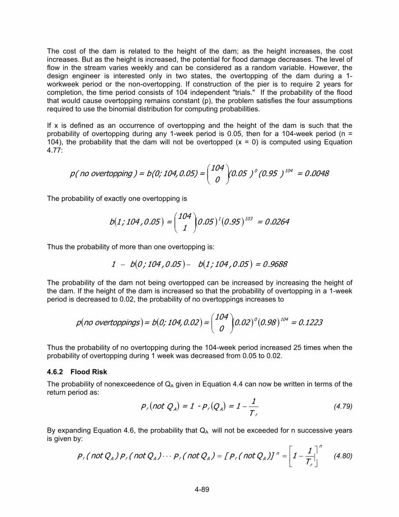
4-89

The cost of the dam is related to the height of the dam; as the height increases, the cost increases. But as the height is increased, the potential for flood damage decreases. The level of flow in the stream varies weekly and can be considered as a random variable. However, the design engineer is interested only in two states, the overtopping of the dam during a 1-workweek period or the non-overtopping. If construction of the pier is to require 2 years for completion, the time period consists of 104 independent "trials." If the probability of the flood that would cause overtopping remains constant (p), the problem satisfies the four assumptions required to use the binomial distribution for computing probabilities. If x is defined as an occurrence of overtopping and the height of the dam is such that the probability of overtopping during any 1-week period is 0.05, then for a 104-week period (n = 104), the probability that the dam will not be overtopped (x = 0) is computed using Equation 4.77:

0048.0 = )(0.95)(0.050

104 = 0.05)104,(0;b = )pingno overtop(p 1040

The probability of exactly one overtopping is

( ) ( ) ( ) 0264.0 = 95.005.01

104 = 05.0,104;1b 1031

Thus the probability of more than one overtopping is: ( ) ( ) 9688.0 = 05.0,104;1 b05.0,104;0 b 1 −− The probability of the dam not being overtopped can be increased by increasing the height of the dam. If the height of the dam is increased so that the probability of overtopping in a 1-week period is decreased to 0.02, the probability of no overtoppings increases to

( ) ( ) ( ) ( ) 0.1223 = 0.980.020

104 =0.02104,0;b = gsovertoppin nop 1040

Thus the probability of no overtopping during the 104-week period increased 25 times when the probability of overtopping during 1 week was decreased from 0.05 to 0.02.

4.6.2 Flood Risk The probability of nonexceedence of QA given in Equation 4.4 can now be written in terms of the return period as:

( ) ( )T11 = QP -1 = Qnot P

rArAr − (4.79)

By expanding Equation 4.6, the probability that QA will not be exceeded for n successive years is given by:

n

r

nArArArAr T

11)]Qnot(P[)Qnot(P)Qnot(P)Qnot(P

−==⋅⋅⋅ (4.80)

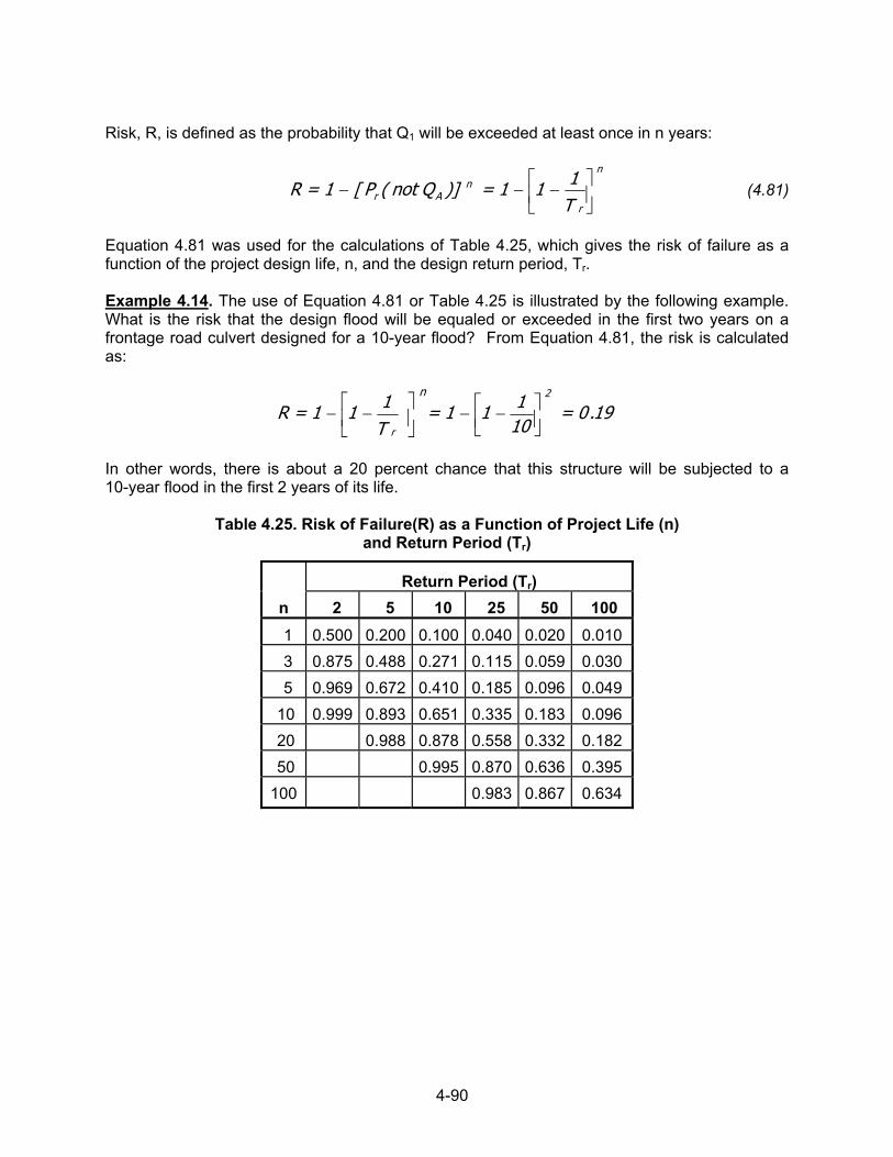
4-90

Risk, R, is defined as the probability that Q1 will be exceeded at least once in n years:

n

r

nAr

T111 = )]Qnot(P[1R =

−−− (4.81)

Equation 4.81 was used for the calculations of Table 4.25, which gives the risk of failure as a function of the project design life, n, and the design return period, Tr. Example 4.14. The use of Equation 4.81 or Table 4.25 is illustrated by the following example. What is the risk that the design flood will be equaled or exceeded in the first two years on a frontage road culvert designed for a 10-year flood? From Equation 4.81, the risk is calculated as:

19.0 = 10111=

T111R =

2

r

n

−−

−−

In other words, there is about a 20 percent chance that this structure will be subjected to a 10-year flood in the first 2 years of its life.

Table 4.25. Risk of Failure(R) as a Function of Project Life (n) and Return Period (Tr)

Return Period (Tr)

n

2

5

10

25

50

100

1 0.500

0.200

0.100

0.040

0.020

0.010

3 0.875

0.488

0.271

0.115

0.059

0.030

5 0.969

0.672

0.410

0.185

0.096

0.049

10 0.999

0.893

0.651

0.335

0.183

0.096

20

0.988

0.878

0.558

0.332

0.182

50

0.995

0.870

0.636

0.395

100

0.983

0.867

0.634