Embed Size (px)
Citation preview

Conservation laws Upwind schemes Clawpack solver WENO solver MHD solver References
Lecture 2Hyperbolic AMROC solvers
Course Block-structured Adaptive Mesh Refinement in C++
Ralf DeiterdingUniversity of Southampton
Engineering and the EnvironmentHighfield Campus, Southampton SO17 1BJ, UK
E-mail: [email protected]
Hyperbolic AMROC solvers 1

Conservation laws Upwind schemes Clawpack solver WENO solver MHD solver References
Outline
Conservation lawsBasics of finite volume methodsSplitting methods, second derivatives
Upwind schemesFlux-difference splittingFlux-vector splittingHigh-resolution methods
Clawpack solverAMR examplesSoftware construction
WENO solverLarge-eddy simulationSoftware construction
MHD solverIdeal magneto-hydrodynamics simulationSoftware design
Hyperbolic AMROC solvers 2

Conservation laws Upwind schemes Clawpack solver WENO solver MHD solver References
Outline
Conservation lawsBasics of finite volume methodsSplitting methods, second derivatives
Upwind schemesFlux-difference splittingFlux-vector splittingHigh-resolution methods
Clawpack solverAMR examplesSoftware construction
WENO solverLarge-eddy simulationSoftware construction
MHD solverIdeal magneto-hydrodynamics simulationSoftware design
Hyperbolic AMROC solvers 3

Conservation laws Upwind schemes Clawpack solver WENO solver MHD solver References
Basics of finite volume methods
Hyperbolic Conservation Laws
∂
∂tq(x, t) +
d∑n=1
∂
∂xnfn(q(x, t)) = 0 , D ⊂ (x, t) ∈ Rd × R+
0
q = q(x, t) ∈ S ⊂ RM - vector of state, fn(q) ∈ C1(S ,RM ) - flux functions,s(q) ∈ C1(S ,RM ) - source term
Definition (Hyperbolicity)
A(q, ν) = ν1A1(q) + · · ·+ νd Ad (q) with An(q) = ∂fn(q)/∂q has M realeigenvalues λ1(q, ν) ≤ ... ≤ λM (q, ν) and M linear independent righteigenvectors rm(q, ν).
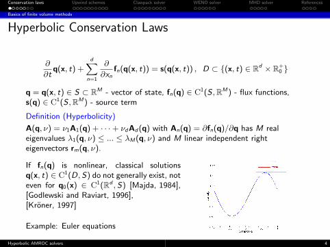
If fn(q) is nonlinear, classical solutionsq(x, t) ∈ C1(D, S) do not generally exist, noteven for q0(x) ∈ C1(Rd , S) [Majda, 1984],[Godlewski and Raviart, 1996],[Kroner, 1997]
Example: Euler equations
Hyperbolic AMROC solvers 4

Conservation laws Upwind schemes Clawpack solver WENO solver MHD solver References
Basics of finite volume methods
Hyperbolic Conservation Laws
∂
∂tq(x, t) +
d∑n=1
∂
∂xnfn(q(x, t)) = 0 , D ⊂ (x, t) ∈ Rd × R+
0
q = q(x, t) ∈ S ⊂ RM - vector of state, fn(q) ∈ C1(S ,RM ) - flux functions,
s(q) ∈ C1(S ,RM ) - source term
Definition (Hyperbolicity)
A(q, ν) = ν1A1(q) + · · ·+ νd Ad (q) with An(q) = ∂fn(q)/∂q has M realeigenvalues λ1(q, ν) ≤ ... ≤ λM (q, ν) and M linear independent righteigenvectors rm(q, ν).
If fn(q) is nonlinear, classical solutionsq(x, t) ∈ C1(D, S) do not generally exist, noteven for q0(x) ∈ C1(Rd , S) [Majda, 1984],[Godlewski and Raviart, 1996],[Kroner, 1997]
Example: Euler equations
Hyperbolic AMROC solvers 4

Conservation laws Upwind schemes Clawpack solver WENO solver MHD solver References
Basics of finite volume methods
Hyperbolic Conservation Laws
∂
∂tq(x, t) +
d∑n=1
∂
∂xnfn(q(x, t)) = s(q(x, t)) , D ⊂ (x, t) ∈ Rd × R+
0
q = q(x, t) ∈ S ⊂ RM - vector of state, fn(q) ∈ C1(S ,RM ) - flux functions,s(q) ∈ C1(S ,RM ) - source term
Definition (Hyperbolicity)
A(q, ν) = ν1A1(q) + · · ·+ νd Ad (q) with An(q) = ∂fn(q)/∂q has M realeigenvalues λ1(q, ν) ≤ ... ≤ λM (q, ν) and M linear independent righteigenvectors rm(q, ν).
If fn(q) is nonlinear, classical solutionsq(x, t) ∈ C1(D, S) do not generally exist, noteven for q0(x) ∈ C1(Rd , S) [Majda, 1984],[Godlewski and Raviart, 1996],[Kroner, 1997]
Example: Euler equations
Hyperbolic AMROC solvers 4

Conservation laws Upwind schemes Clawpack solver WENO solver MHD solver References
Basics of finite volume methods
Weak solutions
Integral form (Gauss’s theorem):∫Ω
q(x, t + ∆t) dx−∫Ω
q(x, t) dx
+d∑
n=1
t+∆t∫t
∫∂Ω
fn(q(o, t))σn(o) do dt =
t+∆t∫t
∫Ω
s(q(x, t)) dx
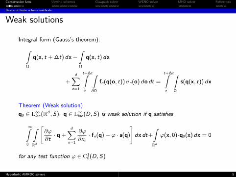
Theorem (Weak solution)
q0 ∈ L∞loc (Rd ,S). q ∈ L∞loc (D, S) is weak solution if q satisfies
∞∫0
∫Rd
[∂ϕ
∂t· q +
d∑n=1
∂ϕ
∂xn· fn(q)− ϕ · s(q)
]dx dt+
∫Rd
ϕ(x, 0)·q0(x) dx = 0
for any test function ϕ ∈ C10(D,S)
Hyperbolic AMROC solvers 5

Conservation laws Upwind schemes Clawpack solver WENO solver MHD solver References
Basics of finite volume methods
Weak solutions
Integral form (Gauss’s theorem):∫Ω
q(x, t + ∆t) dx−∫Ω
q(x, t) dx
+d∑
n=1
t+∆t∫t
∫∂Ω
fn(q(o, t))σn(o) do dt =
t+∆t∫t
∫Ω
s(q(x, t)) dx
Theorem (Weak solution)
q0 ∈ L∞loc (Rd , S). q ∈ L∞loc (D, S) is weak solution if q satisfies
∞∫0
∫Rd
[∂ϕ
∂t· q +
d∑n=1
∂ϕ
∂xn· fn(q)− ϕ · s(q)
]dx dt+
∫Rd
ϕ(x, 0)·q0(x) dx = 0
for any test function ϕ ∈ C10(D, S)
Hyperbolic AMROC solvers 5

Conservation laws Upwind schemes Clawpack solver WENO solver MHD solver References
Basics of finite volume methods
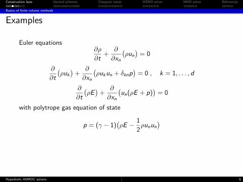
Examples
Euler equations∂ρ
∂t+
∂
∂xn
(ρun
)= 0
∂
∂t
(ρuk
)+
∂
∂xn
(ρuk un + δknp
)= 0 , k = 1, . . . , d
∂
∂t
(ρE
)+
∂
∂xn
(un(ρE + p)
)= 0
with polytrope gas equation of state
p = (γ − 1)(ρE − 1
2ρunun
)have structure
∂tq(x, t) +∇ · f(q(x, t)) = 0
Hyperbolic AMROC solvers 6
Conservation laws Upwind schemes Clawpack solver WENO solver MHD solver References
Basics of finite volume methods
Examples
Euler equations∂ρ
∂t+
∂
∂xn
(ρun
)= 0
∂
∂t
(ρuk
)+
∂
∂xn
(ρuk un + δknp
)= 0 , k = 1, . . . , d
∂
∂t
(ρE
)+
∂
∂xn
(un(ρE + p)
)= 0
with polytrope gas equation of state
p = (γ − 1)(ρE − 1
2ρunun
)
have structure∂tq(x, t) +∇ · f(q(x, t)) = 0
Hyperbolic AMROC solvers 6

Conservation laws Upwind schemes Clawpack solver WENO solver MHD solver References
Basics of finite volume methods
Examples
Euler equations∂ρ
∂t+
∂
∂xn
(ρun
)= 0
∂
∂t
(ρuk
)+
∂
∂xn
(ρuk un + δknp
)= 0 , k = 1, . . . , d
∂
∂t
(ρE
)+
∂
∂xn
(un(ρE + p)
)= 0
with polytrope gas equation of state
p = (γ − 1)(ρE − 1
2ρunun
)have structure
∂tq(x, t) +∇ · f(q(x, t)) = 0
Hyperbolic AMROC solvers 6
Conservation laws Upwind schemes Clawpack solver WENO solver MHD solver References
Basics of finite volume methods
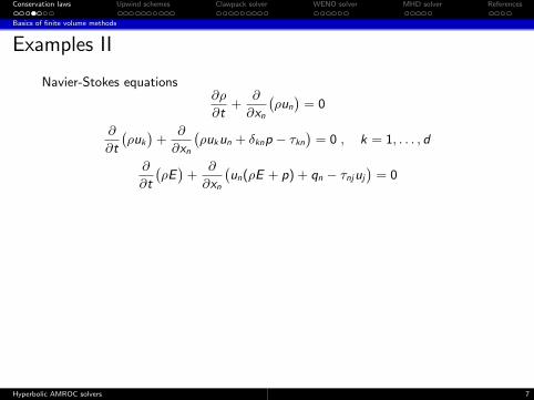
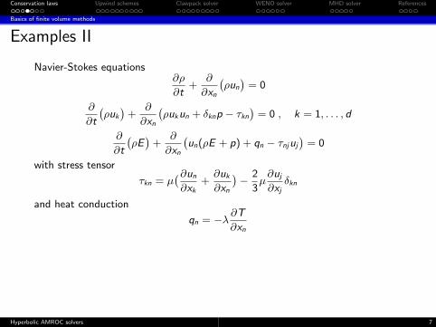
Examples II
Navier-Stokes equations∂ρ
∂t+
∂
∂xn
(ρun
)= 0
∂
∂t
(ρuk
)+
∂
∂xn
(ρuk un + δknp − τkn
)= 0 , k = 1, . . . , d
∂
∂t
(ρE)
+∂
∂xn
(un(ρE + p) + qn − τnj uj
)= 0
with stress tensor
τkn = µ(∂un
∂xk+∂uk
∂xn
)− 2
3µ∂uj
∂xjδkn
and heat conduction
qn = −λ∂T
∂xn
have structure
∂tq(x, t) +∇ · f(q(x, t)) +∇ · h(q(x, t),∇q(x, t)) = 0
Type can be either hyperbolic or parabolic
Hyperbolic AMROC solvers 7
Conservation laws Upwind schemes Clawpack solver WENO solver MHD solver References
Basics of finite volume methods
Examples II
Navier-Stokes equations∂ρ
∂t+
∂
∂xn
(ρun
)= 0
∂
∂t
(ρuk
)+
∂
∂xn
(ρuk un + δknp − τkn
)= 0 , k = 1, . . . , d
∂
∂t
(ρE)
+∂
∂xn
(un(ρE + p) + qn − τnj uj
)= 0
with stress tensor
τkn = µ(∂un
∂xk+∂uk
∂xn
)− 2
3µ∂uj
∂xjδkn
and heat conduction
qn = −λ∂T
∂xn
have structure
∂tq(x, t) +∇ · f(q(x, t)) +∇ · h(q(x, t),∇q(x, t)) = 0
Type can be either hyperbolic or parabolic
Hyperbolic AMROC solvers 7
Conservation laws Upwind schemes Clawpack solver WENO solver MHD solver References
Basics of finite volume methods
Derivation
Assume ∂t q + ∂x f(q) + ∂x h(q(·, ∂x q)) = s(q)
Time discretization tn = n∆t, discrete volumesIj = [xj − 1
2∆x , xj + 1
2∆x[=: [xj−1/2, xj+1/2[
Using approximations Qj (t) ≈1
|Ij |
∫Ij
q(x, t) dx , s(Qj (t)) ≈1
|Ij |
∫Ij
s(q(x, t)) dx
and numerical fluxes
F(Qj (t),Qj+1(t)
)≈ f(q(xj+1/2, t)), H
(Qj (t),Qj+1(t)
)≈ h(q(xj+1/2, t),∇q(xj+1/2, t))
yields after integration (Gauss theorem)
Qj (tn+1) = Qj (tn)−1
∆x
tn+1∫
tn
[F (Qj (t),Qj+1(t))− F (Qj−1(t),Qj (t))] dt−
1
∆x
tn+1∫
tn
[H (Qj (t),Qj+1(t))− H (Qj−1(t),Qj (t))] dt +
tn+1∫
tn
s(Qj (t)) dt
For instance:
Qn+1j = Qn
j −∆t
∆x
[F(
Qnj ,Qn
j+1
)− F
(Qn
j−1,Qnj
)]−
∆t
∆x
[H(
Qnj ,Qn
j+1
)− H
(Qn
j−1,Qnj
)]+ ∆ts(Qn
j ) dt
Hyperbolic AMROC solvers 8

Conservation laws Upwind schemes Clawpack solver WENO solver MHD solver References
Splitting methods, second derivatives
Splitting methods
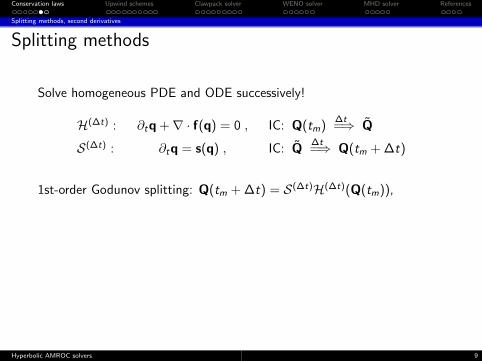
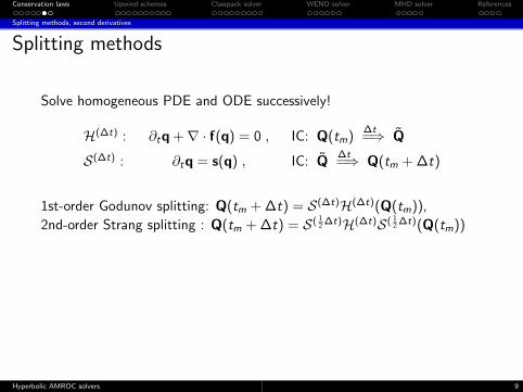
Solve homogeneous PDE and ODE successively!
H(∆t) : ∂tq +∇ · f(q) = 0 , IC: Q(tm)∆t=⇒ Q
S(∆t) : ∂tq = s(q) , IC: Q∆t=⇒ Q(tm + ∆t)
1st-order Godunov splitting: Q(tm + ∆t) = S(∆t)H(∆t)(Q(tm)),
2nd-order Strang splitting : Q(tm + ∆t) = S( 12 ∆t)H(∆t)S( 1
2 ∆t)(Q(tm))
1st-order dimensional splitting for H(·):
X (∆t)1 : ∂tq + ∂x1 f1(q) = 0 , IC: Q(tm)
∆t=⇒ Q1/2
X (∆t)2 : ∂tq + ∂x2 f2(q) = 0 , IC: Q1/2 ∆t
=⇒ Q
[Toro, 1999]
Hyperbolic AMROC solvers 9
Conservation laws Upwind schemes Clawpack solver WENO solver MHD solver References
Splitting methods, second derivatives
Splitting methods
Solve homogeneous PDE and ODE successively!
H(∆t) : ∂tq +∇ · f(q) = 0 , IC: Q(tm)∆t=⇒ Q
S(∆t) : ∂tq = s(q) , IC: Q∆t=⇒ Q(tm + ∆t)
1st-order Godunov splitting: Q(tm + ∆t) = S(∆t)H(∆t)(Q(tm)),
2nd-order Strang splitting : Q(tm + ∆t) = S( 12 ∆t)H(∆t)S( 1
2 ∆t)(Q(tm))
1st-order dimensional splitting for H(·):
X (∆t)1 : ∂tq + ∂x1 f1(q) = 0 , IC: Q(tm)
∆t=⇒ Q1/2
X (∆t)2 : ∂tq + ∂x2 f2(q) = 0 , IC: Q1/2 ∆t
=⇒ Q
[Toro, 1999]
Hyperbolic AMROC solvers 9

Conservation laws Upwind schemes Clawpack solver WENO solver MHD solver References
Splitting methods, second derivatives
Conservative scheme for diffusion equation
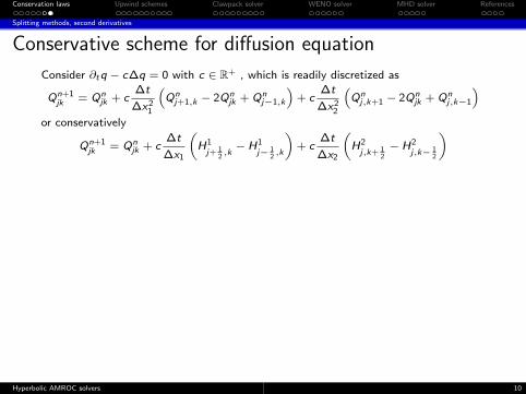
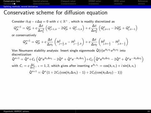
Consider ∂t q − c∆q = 0 with c ∈ R+
, which is readily discretized as
Qn+1jk = Qn
jk + c∆t
∆x21
(Qn
j+1,k − 2Qnjk + Qn
j−1,k
)+ c
∆t
∆x22
(Qn
j,k+1 − 2Qnjk + Qn
j,k−1
)or conservatively
Qn+1jk = Qn
jk + c∆t
∆x1
(H1
j+ 12,k− H1
j− 12,k
)+ c
∆t
∆x2
(H2
j,k+ 12
− H2j,k− 1
2
)Von Neumann stability analysis: Insert single eigenmode Q(t)e ik1x1 e ik2x2 intodiscretization
Qn+1 = Qn+C1
(Qne ik1∆x1 − 2Qn + Qne−ik1∆x1
)+C2
(Qne ik2∆x2 − 2Qn + Qne−ik2∆x2
)with Cι = c ∆t
∆x2ι, ι = 1, 2, which gives after inserting e ikιxι = cos(kιxι) + i sin(kιxι)
Qn+1 = Qn (1 + 2C1(cos(k1∆x1)− 1) + 2C2(cos(k2∆x2)− 1))
Stability requires
|1 + 2C1(cos(k1∆x1)− 1) + 2C2(cos(k2∆x2)− 1)| ≤ 1
i.e.|1− 4C1 − 4C2| ≤ 1
from which we derive the stability condition
0 ≤ c
(∆t
∆x21
+∆t
∆x22
)≤
1
2
Hyperbolic AMROC solvers 10

Conservation laws Upwind schemes Clawpack solver WENO solver MHD solver References
Splitting methods, second derivatives
Conservative scheme for diffusion equation
Consider ∂t q − c∆q = 0 with c ∈ R+ , which is readily discretized as
Qn+1jk = Qn
jk + c∆t
∆x21
(Qn
j+1,k − 2Qnjk + Qn
j−1,k
)+ c
∆t
∆x22
(Qn
j,k+1 − 2Qnjk + Qn
j,k−1
)
or conservatively
Qn+1jk = Qn
jk + c∆t
∆x1
(H1
j+ 12,k− H1
j− 12,k
)+ c
∆t
∆x2
(H2
j,k+ 12
− H2j,k− 1
2
)Von Neumann stability analysis: Insert single eigenmode Q(t)e ik1x1 e ik2x2 intodiscretization
Qn+1 = Qn+C1
(Qne ik1∆x1 − 2Qn + Qne−ik1∆x1
)+C2
(Qne ik2∆x2 − 2Qn + Qne−ik2∆x2
)with Cι = c ∆t
∆x2ι, ι = 1, 2, which gives after inserting e ikιxι = cos(kιxι) + i sin(kιxι)
Qn+1 = Qn (1 + 2C1(cos(k1∆x1)− 1) + 2C2(cos(k2∆x2)− 1))
Stability requires
|1 + 2C1(cos(k1∆x1)− 1) + 2C2(cos(k2∆x2)− 1)| ≤ 1
i.e.|1− 4C1 − 4C2| ≤ 1
from which we derive the stability condition
0 ≤ c
(∆t
∆x21
+∆t
∆x22
)≤
1
2
Hyperbolic AMROC solvers 10
Conservation laws Upwind schemes Clawpack solver WENO solver MHD solver References
Splitting methods, second derivatives
Conservative scheme for diffusion equation
Consider ∂t q − c∆q = 0 with c ∈ R+ , which is readily discretized as
Qn+1jk = Qn
jk + c∆t
∆x21
(Qn
j+1,k − 2Qnjk + Qn
j−1,k
)+ c
∆t
∆x22
(Qn
j,k+1 − 2Qnjk + Qn
j,k−1
)or conservatively
Qn+1jk = Qn
jk + c∆t
∆x1
(H1
j+ 12,k− H1
j− 12,k
)+ c
∆t
∆x2
(H2
j,k+ 12
− H2j,k− 1
2
)
Von Neumann stability analysis: Insert single eigenmode Q(t)e ik1x1 e ik2x2 intodiscretization
Qn+1 = Qn+C1
(Qne ik1∆x1 − 2Qn + Qne−ik1∆x1
)+C2
(Qne ik2∆x2 − 2Qn + Qne−ik2∆x2
)with Cι = c ∆t
∆x2ι, ι = 1, 2, which gives after inserting e ikιxι = cos(kιxι) + i sin(kιxι)
Qn+1 = Qn (1 + 2C1(cos(k1∆x1)− 1) + 2C2(cos(k2∆x2)− 1))
Stability requires
|1 + 2C1(cos(k1∆x1)− 1) + 2C2(cos(k2∆x2)− 1)| ≤ 1
i.e.|1− 4C1 − 4C2| ≤ 1
from which we derive the stability condition
0 ≤ c
(∆t
∆x21
+∆t
∆x22
)≤
1
2
Hyperbolic AMROC solvers 10

Conservation laws Upwind schemes Clawpack solver WENO solver MHD solver References
Splitting methods, second derivatives
Conservative scheme for diffusion equation
Consider ∂t q − c∆q = 0 with c ∈ R+ , which is readily discretized as
Qn+1jk = Qn
jk + c∆t
∆x21
(Qn
j+1,k − 2Qnjk + Qn
j−1,k
)+ c
∆t
∆x22
(Qn
j,k+1 − 2Qnjk + Qn
j,k−1
)or conservatively
Qn+1jk = Qn
jk + c∆t
∆x1
(H1
j+ 12,k− H1
j− 12,k
)+ c
∆t
∆x2
(H2
j,k+ 12
− H2j,k− 1
2
)Von Neumann stability analysis: Insert single eigenmode Q(t)e ik1x1 e ik2x2 intodiscretization
Qn+1 = Qn+C1
(Qne ik1∆x1 − 2Qn + Qne−ik1∆x1
)+C2
(Qne ik2∆x2 − 2Qn + Qne−ik2∆x2
)with Cι = c ∆t
∆x2ι, ι = 1, 2,
which gives after inserting e ikιxι = cos(kιxι) + i sin(kιxι)
Qn+1 = Qn (1 + 2C1(cos(k1∆x1)− 1) + 2C2(cos(k2∆x2)− 1))
Stability requires
|1 + 2C1(cos(k1∆x1)− 1) + 2C2(cos(k2∆x2)− 1)| ≤ 1
i.e.|1− 4C1 − 4C2| ≤ 1
from which we derive the stability condition
0 ≤ c
(∆t
∆x21
+∆t
∆x22
)≤
1
2
Hyperbolic AMROC solvers 10
Conservation laws Upwind schemes Clawpack solver WENO solver MHD solver References
Splitting methods, second derivatives
Conservative scheme for diffusion equation
Consider ∂t q − c∆q = 0 with c ∈ R+ , which is readily discretized as
Qn+1jk = Qn
jk + c∆t
∆x21
(Qn
j+1,k − 2Qnjk + Qn
j−1,k
)+ c
∆t
∆x22
(Qn
j,k+1 − 2Qnjk + Qn
j,k−1
)or conservatively
Qn+1jk = Qn
jk + c∆t
∆x1
(H1
j+ 12,k− H1
j− 12,k
)+ c
∆t
∆x2
(H2
j,k+ 12
− H2j,k− 1
2
)Von Neumann stability analysis: Insert single eigenmode Q(t)e ik1x1 e ik2x2 intodiscretization
Qn+1 = Qn+C1
(Qne ik1∆x1 − 2Qn + Qne−ik1∆x1
)+C2
(Qne ik2∆x2 − 2Qn + Qne−ik2∆x2
)with Cι = c ∆t
∆x2ι, ι = 1, 2, which gives after inserting e ikιxι = cos(kιxι) + i sin(kιxι)
Qn+1 = Qn (1 + 2C1(cos(k1∆x1)− 1) + 2C2(cos(k2∆x2)− 1))
Stability requires
|1 + 2C1(cos(k1∆x1)− 1) + 2C2(cos(k2∆x2)− 1)| ≤ 1
i.e.|1− 4C1 − 4C2| ≤ 1
from which we derive the stability condition
0 ≤ c
(∆t
∆x21
+∆t
∆x22
)≤
1
2
Hyperbolic AMROC solvers 10

Conservation laws Upwind schemes Clawpack solver WENO solver MHD solver References
Splitting methods, second derivatives
Conservative scheme for diffusion equation
Consider ∂t q − c∆q = 0 with c ∈ R+ , which is readily discretized as
Qn+1jk = Qn
jk + c∆t
∆x21
(Qn
j+1,k − 2Qnjk + Qn
j−1,k
)+ c
∆t
∆x22
(Qn
j,k+1 − 2Qnjk + Qn
j,k−1
)or conservatively
Qn+1jk = Qn
jk + c∆t
∆x1
(H1
j+ 12,k− H1
j− 12,k
)+ c
∆t
∆x2
(H2
j,k+ 12
− H2j,k− 1
2
)Von Neumann stability analysis: Insert single eigenmode Q(t)e ik1x1 e ik2x2 intodiscretization
Qn+1 = Qn+C1
(Qne ik1∆x1 − 2Qn + Qne−ik1∆x1
)+C2
(Qne ik2∆x2 − 2Qn + Qne−ik2∆x2
)with Cι = c ∆t
∆x2ι, ι = 1, 2, which gives after inserting e ikιxι = cos(kιxι) + i sin(kιxι)
Qn+1 = Qn (1 + 2C1(cos(k1∆x1)− 1) + 2C2(cos(k2∆x2)− 1))
Stability requires
|1 + 2C1(cos(k1∆x1)− 1) + 2C2(cos(k2∆x2)− 1)| ≤ 1
i.e.|1− 4C1 − 4C2| ≤ 1
from which we derive the stability condition
0 ≤ c
(∆t
∆x21
+∆t
∆x22
)≤
1
2
Hyperbolic AMROC solvers 10

Conservation laws Upwind schemes Clawpack solver WENO solver MHD solver References
Outline
Conservation lawsBasics of finite volume methodsSplitting methods, second derivatives
Upwind schemesFlux-difference splittingFlux-vector splittingHigh-resolution methods
Clawpack solverAMR examplesSoftware construction
WENO solverLarge-eddy simulationSoftware construction
MHD solverIdeal magneto-hydrodynamics simulationSoftware design
Hyperbolic AMROC solvers 11

Conservation laws Upwind schemes Clawpack solver WENO solver MHD solver References
Flux-difference splitting
Linear upwind schemes
Consider Riemann problem
∂
∂tq(x , t)+A
∂
∂xq(x , t) = 0 , x ∈ R , t > 0
Has exact solutionx
t
0
. . . . .
qR
=M∑
m=1
βm rmqL
=M∑
m=1
δm rm
β1r1 +M∑
m=2
δm rm
M−1∑
m=1
βm rm + δM rM
q(x , t) = qL
+∑
λm<x/t
amrm = qR−
∑λm≥x/t
amrm =∑
λm≥x/t
δmrm +∑
λm<x/t
βmrm
Use Riemann problem to evaluate numerical flux F(qL, q
R) := f(q(0, t)) = Aq(0, t) as
F(qL, q
R) = Aq
L+∑λm<0
amλmrm = AqR−∑λm≥0
amλmrm =∑λm≥0
δmλmrm+∑λm<0
βmλmrm
Use λ+m = max(λm, 0) , λ−m = min(λm, 0)
to define Λ+ := diag(λ+1 , . . . , λ
+M ) , Λ− := diag(λ−1 , . . . , λ
−M )
and A+ := R Λ+ R−1 , A− := R Λ− R−1 which gives
F(qL, q
R) = Aq
L+ A−∆q = Aq
R− A+∆q = A+q
L+ A−q
R
with ∆q = qR− q
L
Hyperbolic AMROC solvers 12

Conservation laws Upwind schemes Clawpack solver WENO solver MHD solver References
Flux-difference splitting
Flux difference splitting
Godunov-type scheme with ∆Qnj+1/2 = Qn
j+1 −Qnj
Qn+1j = Qn
j −∆t
∆x
(A−∆Qn
j+1/2 + A+∆Qnj−1/2
)
Use linearization f(q) = A(qL,q
R)q and construct scheme for nonlinear
problem as
Qn+1j = Qn
j −∆t
∆x
(A−(Qn
j ,Qnj+1)∆Qn
j+ 12
+ A+(Qnj−1,Q
nj )∆Qn
j− 12
)stability condition
maxj∈Z|λm,j+ 1
2|∆t
∆x≤ 1 , for all m = 1, . . . ,M
[LeVeque, 1992]
Hyperbolic AMROC solvers 13

Conservation laws Upwind schemes Clawpack solver WENO solver MHD solver References
Flux-difference splitting
Flux difference splitting
Godunov-type scheme with ∆Qnj+1/2 = Qn
j+1 −Qnj
Qn+1j = Qn
j −∆t
∆x
(A−∆Qn
j+1/2 + A+∆Qnj−1/2
)Use linearization f(q) = A(q
L,q
R)q and construct scheme for nonlinear
problem as
Qn+1j = Qn
j −∆t
∆x
(A−(Qn
j ,Qnj+1)∆Qn
j+ 12
+ A+(Qnj−1,Q
nj )∆Qn
j− 12
)
stability condition
maxj∈Z|λm,j+ 1
2|∆t
∆x≤ 1 , for all m = 1, . . . ,M
[LeVeque, 1992]
Hyperbolic AMROC solvers 13

Conservation laws Upwind schemes Clawpack solver WENO solver MHD solver References
Flux-difference splitting
Flux difference splitting
Godunov-type scheme with ∆Qnj+1/2 = Qn
j+1 −Qnj
Qn+1j = Qn
j −∆t
∆x
(A−∆Qn
j+1/2 + A+∆Qnj−1/2
)Use linearization f(q) = A(q
L,q
R)q and construct scheme for nonlinear
problem as
Qn+1j = Qn
j −∆t
∆x
(A−(Qn
j ,Qnj+1)∆Qn
j+ 12
+ A+(Qnj−1,Q
nj )∆Qn
j− 12
)stability condition
maxj∈Z|λm,j+ 1
2|∆t
∆x≤ 1 , for all m = 1, . . . ,M
[LeVeque, 1992]
Hyperbolic AMROC solvers 13

Conservation laws Upwind schemes Clawpack solver WENO solver MHD solver References
Flux-difference splitting
Roe’s approximate Riemann solver
Choosing A(qL, q
R) [Roe, 1981]:
(i) A(qL, q
R) has real eigenvalues
(ii) A(qL, q
R)→ ∂f(q)
∂qas q
L, q
R→ q
(iii) A(qL, q
R)∆q = f(q
R)− f(q
L)
ql qrtn
tn+1
For Euler equations:
ρ =
√ρLρR +
√ρRρL√
ρL +√ρR
=√ρLρR and v =
√ρLvL +
√ρR vR√
ρL +√ρR
for v = un,H
Wave decomposition: ∆q = qr − ql
=∑
m
am rm
F(qL, q
R) = f(q
L) +
∑λm<0
λm am rm = f(qR
)−∑λm≥0
λm am rm
=1
2
(f(q
L) + f(q
R)−
∑m
|λm| am rm
)
Hyperbolic AMROC solvers 14

Conservation laws Upwind schemes Clawpack solver WENO solver MHD solver References
Flux-difference splitting
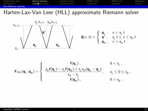
Harten-Lax-Van Leer (HLL) approximate Riemann solver
q⋆
qL
qR
tn
tn+1
sLtn+1 s
Rtn+1
q(x , t) =
q
L, x < s
Lt
q? , sL
t ≤ x ≤ sR
tq
R, x > s
Rt
FHLL(qL, q
R) =
f(q
L) , 0 < s
L,
sR
f(qL
)− sLf(q
R) + s
Ls
R(q
R− q
L)
sR− s
L
, sL≤ 0 ≤ s
R,
f(qR
) , 0 > sR,
Euler equations:
sL
= min(u1,L − cL, u1,R − cR ) , sR
= max(u1,L + cl , u1,R + cR )
[Toro, 1999], HLLC: [Toro et al., 1994]
Hyperbolic AMROC solvers 15
Conservation laws Upwind schemes Clawpack solver WENO solver MHD solver References
Flux-difference splitting
Harten-Lax-Van Leer (HLL) approximate Riemann solver
q⋆
qL
qR
tn
tn+1
sLtn+1 s
Rtn+1
q(x , t) =
q
L, x < s
Lt
q? , sL
t ≤ x ≤ sR
tq
R, x > s
Rt
FHLL(qL, q
R) =
f(q
L) , 0 < s
L,
sR
f(qL
)− sLf(q
R) + s
Ls
R(q
R− q
L)
sR− s
L
, sL≤ 0 ≤ s
R,
f(qR
) , 0 > sR,
Euler equations:
sL
= min(u1,L − cL, u1,R − cR ) , sR
= max(u1,L + cl , u1,R + cR )
[Toro, 1999], HLLC: [Toro et al., 1994]
Hyperbolic AMROC solvers 15

Conservation laws Upwind schemes Clawpack solver WENO solver MHD solver References
Flux-vector splitting
Flux vector splitting
Splitting
f(q) = f+(q) + f−(q)
derived under restriction λ+m ≥ 0 and
λ−m ≤ 0 for all m = 1, . . . ,M for
A+(q) =∂f+(q)
∂q, A−(q) =
∂f−(q)
∂q
qL
qR
f−(qL) f+(q
L) f−(q
R) f+(q
R)
F(qL, q
R) = f+(q
L) + f−(q
R)
tl
tl+1
plus reproduction of regular upwinding
f+(q) = f(q) , f−(q) = 0 if λm ≥ 0 for all m = 1, . . . ,Mf+(q) = 0 , f−(q) = f(q) if λm ≤ 0 for all m = 1, . . . ,M
Then useF(q
L, q
R) = f+(q
L) + f−(q
R)
Hyperbolic AMROC solvers 16

Conservation laws Upwind schemes Clawpack solver WENO solver MHD solver References
Flux-vector splitting
Flux vector splitting
Splitting
f(q) = f+(q) + f−(q)
derived under restriction λ+m ≥ 0 and
λ−m ≤ 0 for all m = 1, . . . ,M for
A+(q) =∂f+(q)
∂q, A−(q) =
∂f−(q)
∂q qL
qR
f−(qL) f+(q
L) f−(q
R) f+(q
R)
F(qL, q
R) = f+(q
L) + f−(q
R)
tl
tl+1
plus reproduction of regular upwinding
f+(q) = f(q) , f−(q) = 0 if λm ≥ 0 for all m = 1, . . . ,Mf+(q) = 0 , f−(q) = f(q) if λm ≤ 0 for all m = 1, . . . ,M
Then useF(q
L, q
R) = f+(q
L) + f−(q
R)
Hyperbolic AMROC solvers 16

Conservation laws Upwind schemes Clawpack solver WENO solver MHD solver References
Flux-vector splitting
Steger-Warming
Required f(q) = A(q) q
λ+m =
1
2(λm + |λm|) λ−m =
1
2(λm − |λm|)
A+(q) := R(q) Λ+(q) R−1(q) , A−(q) := R(q) Λ−(q) R−1(q)
Givesf(q) = A+(q) q + A−(q) q
and the numerical flux
F(qL, q
R) = A+(q
L) q
L+ A−(q
R) q
R
Jacobians of the split fluxes are identical to A±(q) only in linear case
∂f±(q)
∂q=∂(A±(q) q
)∂q
= A±(q) +∂A±(q)
Further methods: Van Leer FVS [Toro, 1999], AUSM [Wada and Liou, 1997]
Hyperbolic AMROC solvers 17

Conservation laws Upwind schemes Clawpack solver WENO solver MHD solver References
High-resolution methods
MUSCL slope limiting
Monotone Upwind Schemes for Conservation Laws [van Leer, 1979]
QL
j+ 12
= Qnj
+1
4
[(1− ω) Φ
+
j− 12
∆j− 12
+ (1 + ω) Φ−j+ 1
2
∆j+ 12
],
QR
j− 12
= Qnj−
1
4
[(1− ω) Φ
−j+ 1
2
∆j+ 12
+ (1 + ω) Φ+
j− 12
∆j− 12
]with ∆j−1/2 = Qn
j − Qnj−1, ∆j+1/2 = Qn
j+1 − Qnj .
Φ+
j− 12
:= Φ
(r+
j− 12
), Φ
−j+ 1
2
:= Φ
(r−j+ 1
2
)with r+
j− 12
:=∆j+ 1
2
∆j− 12
, r−j+ 1
2
:=∆j− 1
2
∆j+ 12
and slope limiters, e.g., Minmod
Φ(r) = max(0,min(r , 1))
Using a midpoint rule for temporal integration, e.g.,
Q?j = Qn
j−
1
2
∆t
∆x
(F (Qn
j+1,Qn
j)− F (Qn
j,Qn
j−1))
and constructing limited values from Q? to be used in FV scheme gives a TVDmethod if
1
2
[(1− ω)Φ(r) + (1 + ω) r Φ
(1
r
)]< min(2, 2r)
is satisfied for r > 0. Proof: [Hirsch, 1988]
Hyperbolic AMROC solvers 18

Conservation laws Upwind schemes Clawpack solver WENO solver MHD solver References
High-resolution methods
Wave Propagation with flux limiting
Wave Propagation Method [LeVeque, 1997] is built on the flux differencing approach
A±∆ := A±(qL, q
R)∆q and the waves Wm := am rm, i.e.
A−∆q =∑λm<0
λmWm , A+∆q =∑λm≥0
λmWm
Wave Propagation 1D:
Qn+1 = Qnj −
∆t
∆x
(A−∆j+ 1
2+A+∆j− 1
2
)−
∆t
∆x
(Fj+ 1
2− Fj− 1
2
)with
Fj+ 12
=1
2|A|(
1−∆t
∆x|A|)
∆j+ 12
=1
2
M∑m=1
|λmj+ 1
2
|(
1−∆t
∆x|λm
j+ 12
|)Wm
j+ 12
and wave limiterWm
j+ 12
= Φ(Θmj+ 1
2
)Wmj+ 1
2
with
Θmj+ 1
2
=
amj− 1
2
/amj+ 1
2
, λmj+ 1
2
≥ 0 ,
amj+ 3
2
/amj+ 1
2
, λmj+ 1
2
< 0
Hyperbolic AMROC solvers 19

Conservation laws Upwind schemes Clawpack solver WENO solver MHD solver References
High-resolution methods
Wave Propagation Method in 2D
Writing A±∆j±1/2 := A+∆j±1/2 + Fj±1/2 one can develop a truly two-dimensionalone-step method [Langseth and LeVeque, 2000]
Qn+1jk = Qn
jk −∆t
∆x1
(A−∆j+ 1
2,k −
1
2
∆t
∆x2
[A−B−∆j+1,k+ 1
2+A−B+∆j+1,k− 1
2
]+
A+∆j− 12,k −
1
2
∆t
∆x2
[A+B−∆j−1,k+ 1
2+A+B+∆j−1,k− 1
2
])−
∆t
∆x2
(B−∆j,k+ 1
2−
1
2
∆t
∆x1
[B−A−∆j+ 1
2,k+1 + B−A+∆j− 1
2,k+1
]+
B+∆j,k− 12−
1
2
∆t
∆x1
[B+A−∆j+ 1
2,k−1 + B+A+∆j− 1
2,k−1
])that is stable for
maxj∈Z|λm,j+ 1
2|
∆t
∆x1,max
k∈Z|λm,k+ 1
2|
∆t
∆x2
≤ 1 , for all m = 1, . . . ,M
Hyperbolic AMROC solvers 20
Conservation laws Upwind schemes Clawpack solver WENO solver MHD solver References
High-resolution methods
Further high-resolution methods
Some further high-resolution methods (good overview in [Laney, 1998]):
I FCT: 2nd order [Oran and Boris, 2001]
I ENO/WENO: 3rd order [Shu, 97]
I PPM: 3rd order [Colella and Woodward, 1984]
3rd order methods must make use of strong-stability preserving Runge-Kuttamethods [Gottlieb et al., 2001] for time integration that use a multi-stepupdate
Qυj = αυQn
j + βυ Qυ−1j + γυ
∆t
∆x
(Fj+ 1
2(Qυ−1)− Fj− 1
2(Qυ−1)
)with Q0 := Qn, α1 = 1, β1 = 0; and Qn+1 := QΥ after final stage Υ
Typical storage-efficient SSPRK(3,3):
Q1 = Qn + ∆tF(Qn), Q2 =3
4Qn +
1
4Q1 +
1
4∆tF(Q1),
Qn+1 =1
3Qn +
2
3Q2 +
2
3∆tF(Q2)
Hyperbolic AMROC solvers 21

Conservation laws Upwind schemes Clawpack solver WENO solver MHD solver References
Outline
Conservation lawsBasics of finite volume methodsSplitting methods, second derivatives
Upwind schemesFlux-difference splittingFlux-vector splittingHigh-resolution methods
Clawpack solverAMR examplesSoftware construction
WENO solverLarge-eddy simulationSoftware construction
MHD solverIdeal magneto-hydrodynamics simulationSoftware design
Hyperbolic AMROC solvers 22

Conservation laws Upwind schemes Clawpack solver WENO solver MHD solver References
AMR examples
SAMR accuracy verificationGaussian density shape
ρ(x1, x2) = 1 + e−(√
x21
+x22
R
)2
is advected with constant velocities u1 = u2 ≡ 1,p0 ≡ 1, R = 1/4
I Domain [−1, 1]× [−1, 1], periodicboundary conditions, tend = 2
I Two levels of adaptation with r1,2 = 2,finest level corresponds to N × N uniformgrid
Use locally conservative interpolation
Qlv,w := Ql
ij + f1(Qli+1,j −Ql
i−1,j ) + f2(Qli,j+1 −Ql
i,j−1)
with factor f1 =xv
1,l+1 − x i1,l
2∆x1,l, f2 =
xw2,l+1 − x j
2,l
2∆x2,lto also test flux correction
This prolongation operator is not monotonicity preserving! Only applicable tosmooth problems.code/amroc/doc/html/apps/clawpack_2applications_2euler_22d_2GaussianPulseAdvection_2src_2Problem_8h_source.html
Hyperbolic AMROC solvers 23
Conservation laws Upwind schemes Clawpack solver WENO solver MHD solver References
AMR examples
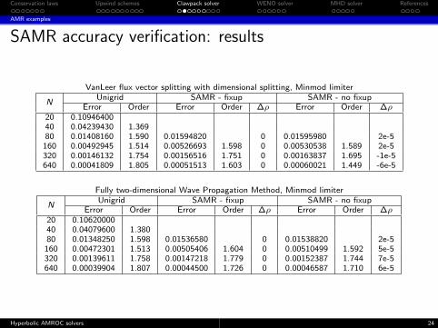
SAMR accuracy verification: results
VanLeer flux vector splitting with dimensional splitting, Minmod limiter
NUnigrid SAMR - fixup SAMR - no fixup
Error Order Error Order ∆ρ Error Order ∆ρ20 0.1094640040 0.04239430 1.36980 0.01408160 1.590 0.01594820 0 0.01595980 2e-5
160 0.00492945 1.514 0.00526693 1.598 0 0.00530538 1.589 2e-5320 0.00146132 1.754 0.00156516 1.751 0 0.00163837 1.695 -1e-5640 0.00041809 1.805 0.00051513 1.603 0 0.00060021 1.449 -6e-5
Fully two-dimensional Wave Propagation Method, Minmod limiter
NUnigrid SAMR - fixup SAMR - no fixup
Error Order Error Order ∆ρ Error Order ∆ρ20 0.1062000040 0.04079600 1.38080 0.01348250 1.598 0.01536580 0 0.01538820 2e-5
160 0.00472301 1.513 0.00505406 1.604 0 0.00510499 1.592 5e-5320 0.00139611 1.758 0.00147218 1.779 0 0.00152387 1.744 7e-5640 0.00039904 1.807 0.00044500 1.726 0 0.00046587 1.710 6e-5
Hyperbolic AMROC solvers 24

Conservation laws Upwind schemes Clawpack solver WENO solver MHD solver References
AMR examples
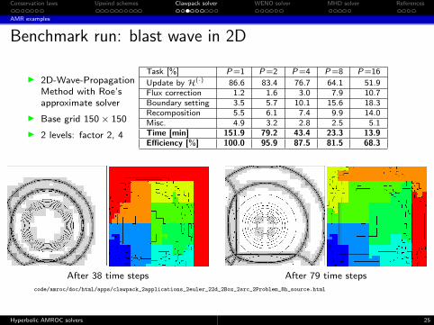
Benchmark run: blast wave in 2D
I 2D-Wave-PropagationMethod with Roe’sapproximate solver
I Base grid 150× 150
I 2 levels: factor 2, 4
Task [%] P =1 P =2 P =4 P =8 P =16
Update by H(·) 86.6 83.4 76.7 64.1 51.9Flux correction 1.2 1.6 3.0 7.9 10.7Boundary setting 3.5 5.7 10.1 15.6 18.3Recomposition 5.5 6.1 7.4 9.9 14.0Misc. 4.9 3.2 2.8 2.5 5.1Time [min] 151.9 79.2 43.4 23.3 13.9Efficiency [%] 100.0 95.9 87.5 81.5 68.3
After 38 time steps After 79 time steps
code/amroc/doc/html/apps/clawpack_2applications_2euler_22d_2Box_2src_2Problem_8h_source.html
Hyperbolic AMROC solvers 25
Conservation laws Upwind schemes Clawpack solver WENO solver MHD solver References
AMR examples
Benchmark run: blast wave in 2D
I 2D-Wave-PropagationMethod with Roe’sapproximate solver
I Base grid 150× 150
I 2 levels: factor 2, 4
Task [%] P =1 P =2 P =4 P =8 P =16
Update by H(·) 86.6 83.4 76.7 64.1 51.9Flux correction 1.2 1.6 3.0 7.9 10.7Boundary setting 3.5 5.7 10.1 15.6 18.3Recomposition 5.5 6.1 7.4 9.9 14.0Misc. 4.9 3.2 2.8 2.5 5.1Time [min] 151.9 79.2 43.4 23.3 13.9Efficiency [%] 100.0 95.9 87.5 81.5 68.3
After 38 time steps After 79 time steps
code/amroc/doc/html/apps/clawpack_2applications_2euler_22d_2Box_2src_2Problem_8h_source.html
Hyperbolic AMROC solvers 25

Conservation laws Upwind schemes Clawpack solver WENO solver MHD solver References
AMR examples
Benchmark run 2: point-explosion in 3D
I Benchmark from the Chicagoworkshop on AMR methods,September 2003
I Sedov explosion - energydeposition in sphere of radius 4finest cells
I 3D-Wave-Prop. Method withhybrid Roe-HLL scheme
I Base grid 323
I Refinement factor rl = 2
I Effective resolutions: 1283,2563, 5123, 10243
I Grid generation efficiencyηtol = 85%
I Proper nesting enforced
I Buffer of 1 cell
lmax = 4 solution
lmax = 5 solution
Hyperbolic AMROC solvers 26

Conservation laws Upwind schemes Clawpack solver WENO solver MHD solver References
AMR examples
Benchmark run 2: visualization of refinement
l = 0 l = 1 l = 2
l = 3 l = 4 l = 5
Hyperbolic AMROC solvers 27

Conservation laws Upwind schemes Clawpack solver WENO solver MHD solver References
AMR examples
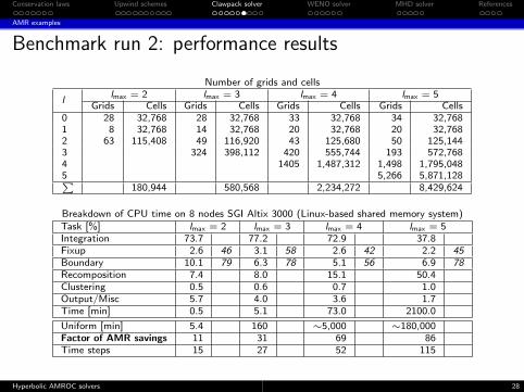
Benchmark run 2: performance results
Number of grids and cells
llmax = 2 lmax = 3 lmax = 4 lmax = 5
Grids Cells Grids Cells Grids Cells Grids Cells0 28 32,768 28 32,768 33 32,768 34 32,7681 8 32,768 14 32,768 20 32,768 20 32,7682 63 115,408 49 116,920 43 125,680 50 125,1443 324 398,112 420 555,744 193 572,7684 1405 1,487,312 1,498 1,795,0485 5,266 5,871,128∑
180,944 580,568 2,234,272 8,429,624
Breakdown of CPU time on 8 nodes SGI Altix 3000 (Linux-based shared memory system)Task [%] lmax = 2 lmax = 3 lmax = 4 lmax = 5Integration 73.7 77.2 72.9 37.8Fixup 2.6 46 3.1 58 2.6 42 2.2 45Boundary 10.1 79 6.3 78 5.1 56 6.9 78Recomposition 7.4 8.0 15.1 50.4Clustering 0.5 0.6 0.7 1.0Output/Misc 5.7 4.0 3.6 1.7Time [min] 0.5 5.1 73.0 2100.0
Uniform [min] 5.4 160 ∼5,000 ∼180,000Factor of AMR savings 11 31 69 86Time steps 15 27 52 115
code/amroc/doc/html/apps/clawpack_2applications_2euler_23d_2Sedov_2src_2Problem_8h_source.html
Hyperbolic AMROC solvers 28
Conservation laws Upwind schemes Clawpack solver WENO solver MHD solver References
AMR examples
Benchmark run 2: performance results
Number of grids and cells
llmax = 2 lmax = 3 lmax = 4 lmax = 5
Grids Cells Grids Cells Grids Cells Grids Cells0 28 32,768 28 32,768 33 32,768 34 32,7681 8 32,768 14 32,768 20 32,768 20 32,7682 63 115,408 49 116,920 43 125,680 50 125,1443 324 398,112 420 555,744 193 572,7684 1405 1,487,312 1,498 1,795,0485 5,266 5,871,128∑
180,944 580,568 2,234,272 8,429,624
Breakdown of CPU time on 8 nodes SGI Altix 3000 (Linux-based shared memory system)Task [%] lmax = 2 lmax = 3 lmax = 4 lmax = 5Integration 73.7 77.2 72.9 37.8Fixup 2.6 46 3.1 58 2.6 42 2.2 45Boundary 10.1 79 6.3 78 5.1 56 6.9 78Recomposition 7.4 8.0 15.1 50.4Clustering 0.5 0.6 0.7 1.0Output/Misc 5.7 4.0 3.6 1.7Time [min] 0.5 5.1 73.0 2100.0
Uniform [min] 5.4 160 ∼5,000 ∼180,000Factor of AMR savings 11 31 69 86Time steps 15 27 52 115
code/amroc/doc/html/apps/clawpack_2applications_2euler_23d_2Sedov_2src_2Problem_8h_source.html
Hyperbolic AMROC solvers 28

Conservation laws Upwind schemes Clawpack solver WENO solver MHD solver References
Software construction
Components
Directory amroc/clawpack/src contains generic Fortran functions:
I ?d/integrator extended: Contains an extended version of Clawpack 3.0by R. LeVeque. The MUSCL approach was added, 3d fully implemented,interfaces have been adjusted for AMROC. These codes are equationindependent.code/amroc/doc/html/clp/files.html
I ?d/equations: Contains equation-specific Riemann solvers, flux functionsas F77 routines.
I ?d/interpolation: Contains patch-wise interpolation and restrictionoperators in F77.
Directory amroc/clawpack contains the generic C++ classes to interface theF77 library from ?d/integrator extended with AMROC:
I ClpIntegrator<VectorType, AuxVectorType, dim >: Interfaces the F77library from ?d/integrator extended to Integrator<VectorType, dim>.Key function to fill is CalculateGrid().code/amroc/doc/html/clp/classClpIntegrator_3_01VectorType_00_01AuxVectorType_00_012_01_4.html
Hyperbolic AMROC solvers 29

Conservation laws Upwind schemes Clawpack solver WENO solver MHD solver References
Software construction
Components - II
I ClpFixup<VectorType, FixupType, AuxVectorType, dim >: Theconservative flux correction is more complex in the waves of the fluxdifference splitting schemes. This specialization ofAMRFixup<VectorType, FixupType, dim>considers this.code/amroc/doc/html/clp/classClpFixup.html
I A generic main program amroc/clawpack/mains/amr main.Cinstantiates Integrator<VectorType, dim>, InitialCondition<VectorType,dim >, BoundaryConditions<VectorType, dim >code/amroc/doc/html/clp/amr__main_8C.html
I Problem.h: Allows simulation-specific alteration in class-libary style byderivation from predefined classes specified in ClpStdProblem.hcode/amroc/doc/html/clp/ClpStdProblem_8h.html
I ClpProblem.h: General include before equation-specific C++ definitionfile is read that defines VectorType and provides Fortran function namesrequired by amroc/amr/F77Interfaces classescode/amroc/doc/html/clp/ClpProblem_8h_source.html code/amroc/doc/html/clp/euler2_8h.html
Hyperbolic AMROC solvers 30

Conservation laws Upwind schemes Clawpack solver WENO solver MHD solver References
Software construction
Functions to link in Makefile.am
Interface objects from amroc/amr/F77Interfaces are used to mimic theinterface of standard Clawpack, which constructs specific simulations by linkingF77 functions. Required functions are:
I init.f: Initial conditions.
I physbd.f: Boundary conditions.
I combl.f: Initialize application specific common blocks.
I $(EQUATION)/rp/rpn.f and rpt.f: Equation-specific Riemann solvers innormal and transverse direction.
I $(EQUATION)/rp/flx.f, $(EQUATION)/rp/rec.f: Flux andreconstruction for MUSCL slope limiting (if used), otherwisedummy-routines/flx.f and dummy-routines/rec.f may be used.
I $(EQUATION)/rp/chk.f: Physical consistency check for debugging.
I src.f: Source term for a splitting method., otherwisedummy-routines/src.f can be linked.
I setaux.f: Set data in an additional patch-wise auxiliary array, otherwisedummy-routines/saux.f can be linked.
Hyperbolic AMROC solvers 31

Conservation laws Upwind schemes Clawpack solver WENO solver MHD solver References
Outline
Conservation lawsBasics of finite volume methodsSplitting methods, second derivatives
Upwind schemesFlux-difference splittingFlux-vector splittingHigh-resolution methods
Clawpack solverAMR examplesSoftware construction
WENO solverLarge-eddy simulationSoftware construction
MHD solverIdeal magneto-hydrodynamics simulationSoftware design
Hyperbolic AMROC solvers 32

Conservation laws Upwind schemes Clawpack solver WENO solver MHD solver References
Large-eddy simulation
Favre-averaged Navier-Stokes equations
∂ρ
∂t+
∂
∂xn
(ρun)
= 0
∂
∂t
(ρuk
)+
∂
∂xn
(ρuk un + δknp − τkn + σkn
)= 0
∂ρE
∂t+
∂
∂xn
(un(ρE + p) + qn − τnj uj + σe
n
)= 0
∂
∂t
(ρYi
)+
∂
∂xn
(ρYi un + J i
n + σin
)= 0
with stress tensor
τkn = µ(∂un
∂xk+∂uk
∂xn
)−
2
3µ∂uj
∂xjδin ,
heat conduction
qn = −λ∂T
∂xn,
and inter-species diffusion
J in = −ρDi
∂Yi
∂xnFavre-filtering
φ =ρφ
ρwith φ(x, t; ∆c ) =
∫Ω
G(x− x′; ∆c )φ(x
′, t)dx
′
Hyperbolic AMROC solvers 33
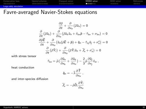
Conservation laws Upwind schemes Clawpack solver WENO solver MHD solver References
Large-eddy simulation
Favre-averaged Navier-Stokes equations
∂ρ
∂t+
∂
∂xn
(ρun)
= 0
∂
∂t
(ρuk
)+
∂
∂xn
(ρuk un + δknp − τkn + σkn
)= 0
∂ρE
∂t+
∂
∂xn
(un(ρE + p) + qn − τnj uj + σe
n
)= 0
∂
∂t
(ρYi
)+
∂
∂xn
(ρYi un + J i
n + σin
)= 0
with stress tensor
τkn = µ(∂un
∂xk+∂uk
∂xn
)−
2
3µ∂uj
∂xjδin ,
heat conduction
qn = −λ∂T
∂xn,
and inter-species diffusion
J in = −ρDi
∂Yi
∂xn
Favre-filtering
φ =ρφ
ρwith φ(x, t; ∆c ) =
∫Ω
G(x− x′; ∆c )φ(x
′, t)dx
′
Hyperbolic AMROC solvers 33

Conservation laws Upwind schemes Clawpack solver WENO solver MHD solver References
Large-eddy simulation
Favre-averaged Navier-Stokes equations
∂ρ
∂t+
∂
∂xn
(ρun)
= 0
∂
∂t
(ρuk
)+
∂
∂xn
(ρuk un + δknp − τkn + σkn
)= 0
∂ρE
∂t+
∂
∂xn
(un(ρE + p) + qn − τnj uj + σe
n
)= 0
∂
∂t
(ρYi
)+
∂
∂xn
(ρYi un + J i
n + σin
)= 0
with stress tensor
τkn = µ(∂un
∂xk+∂uk
∂xn
)−
2
3µ∂uj
∂xjδin ,
heat conduction
qn = −λ∂T
∂xn,
and inter-species diffusion
J in = −ρDi
∂Yi
∂xnFavre-filtering
φ =ρφ
ρwith φ(x, t; ∆c ) =
∫Ω
G(x− x′; ∆c )φ(x
′, t)dx
′
Hyperbolic AMROC solvers 33
Conservation laws Upwind schemes Clawpack solver WENO solver MHD solver References
Large-eddy simulation
Numerical solution approach
I Subgrid terms σkn, σen , σi
n are computed by Pullin’s stretched-vortex model
I Cutoff ∆c is set to local SAMR resolution ∆xl
I It remains to solve the Navier-Stokes equations in the hyperbolic regime
I 3rd order WENO method (hybridized with a tuned centereddifference stencil) for convection
I 2nd order conservative centered differences for diffusion
Example: Cylindrical Richtmyer-Meshkov instability
I Sinusoidal interface between two gases hit byshock wave
I Objective is correctly predict turbulent mixing
I Embedded boundary method used to regularizeapex
I AMR base grid 95× 95× 64 cells, r1,2,3 = 2
I ∼ 70, 000h CPU on 32 AMD 2.5GHZ-quad-corenodes
Hyperbolic AMROC solvers 34

Conservation laws Upwind schemes Clawpack solver WENO solver MHD solver References
Large-eddy simulation
Planar Richtmyer-Meshkov instability
I Perturbed Air-SF6 interface shocked andre-shocked by Mach 1.5 shock
I Containment of turbulence in refinedzones
I 96 CPUs IBM SP2-Power3
I WENO-TCD scheme with LES model
I AMR base grid 172× 56× 56, r1,2 = 2,10M cells in average instead of 3M(uniform)
Task 2ms (%) 5ms (%) 10ms (%)Integration 45.3 65.9 52.0
Boundary setting 44.3 28.6 41.9Flux correction 7.2 3.4 4.1Interpolation 0.9 0.4 0.3
Reorganization 1.6 1.2 1.2Misc. 0.6 0.5 0.5
Max. imbalance 1.25 1.23 1.30
code/amroc/doc/html/apps/weno_2applications_2euler_23d_2RM_
_AirSF6_2src_2Problem_8h_source.html
Hyperbolic AMROC solvers 35

Conservation laws Upwind schemes Clawpack solver WENO solver MHD solver References
Large-eddy simulation
Flux correction for Runge-Kutta method
Recall Runge-Kutta temporal update
Qυj = αυQnj + βυ Qυ−1
j + γυ∆t
∆xk∆Fk (Qυ−1)
rewrite scheme as
Qn+1 = Qn −Υ∑υ=1
ϕυ∆t
∆xk∆Fk (Qυ−1) with ϕυ = γυ
Υ∏ν=υ+1
βν
Flux correction to be used [Pantano et al., 2007]
1. δF1,l+1
i− 12,j
:= −ϕ1F1,l
i− 12,j
(Q0) , δF1,l+1
i− 12,j
:= δF1,l+1
i− 12,j−
Υ∑υ=2
ϕυF1,l
i− 12,j
(Qυ−1)
2. δF1,l+1
i− 12,j
:= δF1,l+1
i− 12,j
+1
r2l+1
rl+1−1∑m=0
Υ∑υ=1
ϕυF1,l+1
v+ 12,w+m
(Qυ−1(t + κ∆tl+1)
)Storage-efficient SSPRK(3,3):
υ αυ βυ γυ ϕυ
1 1 0 1 16
2 34
14
14
16
3 12
23
23
23
Hyperbolic AMROC solvers 36

Conservation laws Upwind schemes Clawpack solver WENO solver MHD solver References
Large-eddy simulation
Flux correction for Runge-Kutta method
Recall Runge-Kutta temporal update
Qυj = αυQnj + βυ Qυ−1
j + γυ∆t
∆xk∆Fk (Qυ−1)
rewrite scheme as
Qn+1 = Qn −Υ∑υ=1
ϕυ∆t
∆xk∆Fk (Qυ−1) with ϕυ = γυ
Υ∏ν=υ+1
βν
Flux correction to be used [Pantano et al., 2007]
1. δF1,l+1
i− 12,j
:= −ϕ1F1,l
i− 12,j
(Q0) , δF1,l+1
i− 12,j
:= δF1,l+1
i− 12,j−
Υ∑υ=2
ϕυF1,l
i− 12,j
(Qυ−1)
2. δF1,l+1
i− 12,j
:= δF1,l+1
i− 12,j
+1
r2l+1
rl+1−1∑m=0
Υ∑υ=1
ϕυF1,l+1
v+ 12,w+m
(Qυ−1(t + κ∆tl+1)
)
Storage-efficient SSPRK(3,3):υ αυ βυ γυ ϕυ
1 1 0 1 16
2 34
14
14
16
3 12
23
23
23
Hyperbolic AMROC solvers 36

Conservation laws Upwind schemes Clawpack solver WENO solver MHD solver References
Large-eddy simulation
Flux correction for Runge-Kutta method
Recall Runge-Kutta temporal update
Qυj = αυQnj + βυ Qυ−1
j + γυ∆t
∆xk∆Fk (Qυ−1)
rewrite scheme as
Qn+1 = Qn −Υ∑υ=1
ϕυ∆t
∆xk∆Fk (Qυ−1) with ϕυ = γυ
Υ∏ν=υ+1
βν
Flux correction to be used [Pantano et al., 2007]
1. δF1,l+1
i− 12,j
:= −ϕ1F1,l
i− 12,j
(Q0) , δF1,l+1
i− 12,j
:= δF1,l+1
i− 12,j−
Υ∑υ=2
ϕυF1,l
i− 12,j
(Qυ−1)
2. δF1,l+1
i− 12,j
:= δF1,l+1
i− 12,j
+1
r2l+1
rl+1−1∑m=0
Υ∑υ=1
ϕυF1,l+1
v+ 12,w+m
(Qυ−1(t + κ∆tl+1)
)Storage-efficient SSPRK(3,3):
υ αυ βυ γυ ϕυ
1 1 0 1 16
2 34
14
14
16
3 12
23
23
23
Hyperbolic AMROC solvers 36

Conservation laws Upwind schemes Clawpack solver WENO solver MHD solver References
Software construction
Components
Directory amroc/weno/src contains the Fortran-90 solver library:
I generic: Implements the hybrid WENO-TCD method for Euler andNavier-Stokes equations, characteristic boundary conditions. Code usesF90 modules.code/amroc/doc/html/weno/files.html
I equations: Contains routines that specify between LES and laminar flow,the criterion for scheme hybridization, source terms handled by splitting.
Directory amroc/weno contains the generic C++ class to interface the F90library with AMROC:
I WENOIntegrator<VectorType, dim >: Interfaces the F90 solver toIntegrator<VectorType, dim>. CalculateGrid() is called separately foreach stage of the Runge-Kutta time integrator.code/amroc/doc/html/weno/classWENOIntegrator.html
I WENOFixup<VectorType, FixupType, dim >: A specializedconservative flux correction that accumulates the correction termsthroughout the stages of the Runge-Kutta time integrator.code/amroc/doc/html/weno/classWENOFixup.html
Hyperbolic AMROC solvers 37
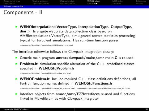
Conservation laws Upwind schemes Clawpack solver WENO solver MHD solver References
Software construction
Components - II
I WENOInterpolation<VectorType, InterpolationType, OutputType,dim >: Is a quite elaborate data collection class based onAMRInterpolation<VectorType, dim>geared toward statistics processingtypical for turbulent simulations. Has run-time function parser.code/amroc/doc/html/weno/classWENOStatistics.html
The interface otherwise follows the Clawpack integration closely:
I Generic main program amroc/clawpack/mains/amr main.C is re-used.
I Problem.h: simulation-specific alteration of the C++ predefined classesspecified in WENOStdProblem.hcode/amroc/doc/html/weno/WENOStdProblem_8h.html
I WENOProblem.h: Include required C++ class definitions definitions, allFortran function names defined in WENOStdFunctions.hcode/amroc/doc/html/weno/WENOProblem_8h_source.html code/amroc/doc/html/weno/WENOStdFunctions_8h.html
I Interface objects from amroc/amr/F77Interfaces re-used and functionslinked in Makefile.am as with Clawpack integrator
Hyperbolic AMROC solvers 38
Conservation laws Upwind schemes Clawpack solver WENO solver MHD solver References
Outline
Conservation lawsBasics of finite volume methodsSplitting methods, second derivatives
Upwind schemesFlux-difference splittingFlux-vector splittingHigh-resolution methods
Clawpack solverAMR examplesSoftware construction
WENO solverLarge-eddy simulationSoftware construction
MHD solverIdeal magneto-hydrodynamics simulationSoftware design
Hyperbolic AMROC solvers 39
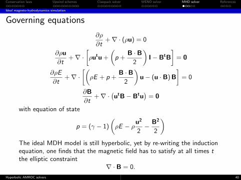
Conservation laws Upwind schemes Clawpack solver WENO solver MHD solver References
Ideal magneto-hydrodynamics simulation
Governing equations
∂ρ
∂t+∇ · (ρu) = 0
∂ρu
∂t+∇ ·
[ρutu +
(p +
B · B2
)I− BtB
]= 0
∂ρE
∂t+∇ ·
[(ρE + p +
B · B2
)u− (u · B) B
]= 0
∂B
∂t+∇ ·
(utB− Btu
)= 0
with equation of state
p = (γ − 1)
(ρE − ρu2
2− B2
2
)The ideal MDH model is still hyperbolic, yet by re-writing the inductionequation, one finds that the magnetic field has to satisfy at all times tthe elliptic constraint
∇ · B = 0.
Hyperbolic AMROC solvers 40

Conservation laws Upwind schemes Clawpack solver WENO solver MHD solver References
Ideal magneto-hydrodynamics simulation
Generalized Lagrangian multipliers for divergence controlHyperbolic-parabolic correction of 2d ideal MHD model [Dedner et al., 2002]:
∂ρ
∂t+∂ρux
∂x+∂ρuy
∂y= 0
∂ (ρux )
∂t+
∂
∂x
[ρu2
x + p
(p +
B · B2
)− B2
x
]+
∂
∂y(ρux uy − Bx By ) = 0
∂ (ρuy )
∂t+
∂
∂x(ρux uy − Bx By ) +
∂
∂y
[ρu2
y + p
(p +
B · B2
)− B2
y
]= 0
∂ (ρuz )
∂t+
∂
∂x(ρuz ux − Bz Bx ) +
∂
∂y(ρuz uy − Bz By ) = 0
∂ρE
∂t+∂
∂x
[(ρE + p +
B · B2
)ux − (u · B) Bx
]+∂
∂y
[(ρE + p +
B · B2
)uy − (u · B) By
]= 0
∂Bx
∂t+∂ψ
∂x+
∂
∂y(uy Bx − By ux ) = 0
∂By
∂t+
∂
∂x(ux By − Bx uy ) +
∂ψ
∂y= 0
∂Bz
∂t+
∂
∂x(ux Bz − Bz ux ) +
∂
∂y(uy Bz − By uz ) = 0
∂ψ
∂t+ c2
h
(∂Bx
∂x+∂By
∂y
)= −
c2h
c2p
ψ
Hyperbolic AMROC solvers 41

Conservation laws Upwind schemes Clawpack solver WENO solver MHD solver References
Ideal magneto-hydrodynamics simulation
Orszag-Tang vortexI Adaptive solution on 50× 50 grid with 4 additional levels refined by rl = 2I Initial condition
ρ(x, y , 0) = γ2, ux (x, y , 0) = − sin(y), uy (x, y , 0) = sin(x), uz (x, y , 0) = 0
p(x, y , 0) = γ, Bx (x, y , 0) = − sin(y), By (x, y , 0) = 2 sin(x), Bz (x, y , 0) = 0
Scaled gradient of ρMulti-resolution criterion with
hierarchical thresholdingcode/amroc/doc/html/apps/mhd_2applications_2eglm_22d_2OrszagTangVortex_2src_2Problem_8h_source.html
Hyperbolic AMROC solvers 42
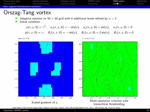
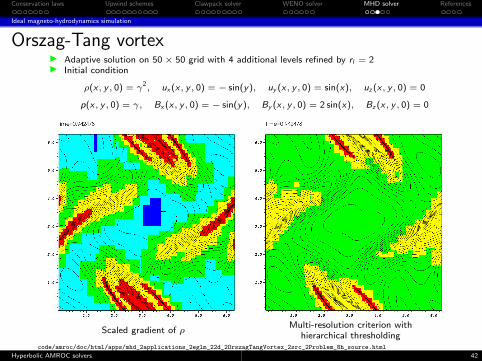
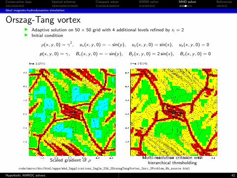

Conservation laws Upwind schemes Clawpack solver WENO solver MHD solver References
Software design
Classes
Directory amroc/mhd contains the integrator that is in C++ throughout:
I EGLM2D<DataType >: GLM method in 2d plus standard initial andboundary conditions. Internal functions for flux evaluation, MUSCLresconstruction, etc. are member functions.code/amroc/doc/html/mhd/classEGLM2D.html
I Is derived from SchemeBase<vector type, dim >, which is designed forthe C++ interface classes in amroc/amr/Interfaces.code/amroc/doc/html/amr/classSchemeBase.html
I amroc/amr/Interfaces: Provides SchemeIntegrator<SchemeType, dim>, SchemeInitialCondition<SchemeType, dim >,SchemeBoundaryCondition<SchemeType, dim > and further interfacesthat use classes derived from SchemeBase<vector type, dim > astemplate parameter. This provides a single-class location for new schemesin C++.code/amroc/doc/html/amr/classSchemeIntegrator.html code/amroc/doc/html/amr/classSchemeInitialCondition.html
I Problem.h: Specific simulation is defined in Problem.h only. Predefinedclasses specified in MHDStdProblem.h and MHDProblem.h similar butsimpler as before.code/amroc/doc/html/mhd/MHDStdProblem_8h.html code/amroc/doc/html/mhd/MHDProblem_8h_source.html
Hyperbolic AMROC solvers 43

Conservation laws Upwind schemes Clawpack solver WENO solver MHD solver References
Software design
Further hyperbolic solvers
I amroc/rim: Riemann invariant manifold method. 2d implementation inF77 with straightforward integration into AMROC.code/amroc/doc/html/rim/files.html
I amroc/balans: 2nd order accurate central difference scheme. 2dimplementation in F77 and excellent template for Fortran schemeincorporation into AMROC.code/amroc/doc/html/balans/files.html
Hyperbolic AMROC solvers 44

Conservation laws Upwind schemes Clawpack solver WENO solver MHD solver References
References
References I
[Colella and Woodward, 1984] Colella, P. and Woodward, P. (1984). The piecewiseparabolic method (PPM) for gas-dynamical simulations. J. Comput. Phys.,54:174–201.
[Dedner et al., 2002] Dedner, A., Kemm, F., Kroner, D., Munz, C.-D., Schnitzer, T.,and Wesenberg, M. (2002). Hyperbolic divergence cleaning for the MHD equations.J. Comput. Phys., 175:645–673.
[Godlewski and Raviart, 1996] Godlewski, E. and Raviart, P.-A. (1996). Numericalapproximation of hyperbolic systems of conservation laws. Springer Verlag, NewYork.
[Gottlieb et al., 2001] Gottlieb, S., Shu, C.-W., and Tadmor, E. (2001). Strongstability-preserving high-order time discretization methods. SIAM Review,43(1):89–112.
[Hirsch, 1988] Hirsch, C. (1988). Numerical computation of internal and externalflows. John Wiley & Sons, Chichester.
[Kroner, 1997] Kroner, D. (1997). Numerical schemes for conservation laws. JohnWiley & Sons and B. G. Teubner, New York, Leipzig.
Hyperbolic AMROC solvers 45

Conservation laws Upwind schemes Clawpack solver WENO solver MHD solver References
References
References II
[Laney, 1998] Laney, C. B. (1998). Computational gasdynamics. Cambridge UniversityPress, Cambridge.
[Langseth and LeVeque, 2000] Langseth, J. and LeVeque, R. (2000). A wavepropagation method for three dimensional conservation laws. J. Comput. Phys.,165:126–166.
[LeVeque, 1992] LeVeque, R. J. (1992). Numerical methods for conservation laws.Birkhauser, Basel.
[LeVeque, 1997] LeVeque, R. J. (1997). Wave propagation algorithms formultidimensional hyperbolic systems. J. Comput. Phys., 131(2):327–353.
[Majda, 1984] Majda, A. (1984). Compressible fluid flow and systems of conservationlaws in several space variables. Applied Mathematical Sciences Vol. 53.Springer-Verlag, New York.
[Oran and Boris, 2001] Oran, E. S. and Boris, J. P. (2001). Numerical simulation ofreactive flow. Cambridge Univ. Press, Cambridge, 2nd edition.
Hyperbolic AMROC solvers 46

Conservation laws Upwind schemes Clawpack solver WENO solver MHD solver References
References
References III
[Pantano et al., 2007] Pantano, C., Deiterding, R., Hill, D. J., and Pullin, D. I.(2007). A low-numerical dissipation patch-based adaptive mesh refinement methodfor large-eddy simulation of compressible flows. J. Comput. Phys., 221(1):63–87.
[Roe, 1981] Roe, P. L. (1981). Approximate Riemann solvers, parameter vectors anddifference schemes. J. Comput. Phys., 43:357–372.
[Shu, 97] Shu, C.-W. (97). Essentially non-oscillatory and weigted essentiallynon-oscillatory schemes for hyperbolic conservation laws. Technical ReportCR-97-206253, NASA.
[Toro, 1999] Toro, E. F. (1999). Riemann solvers and numerical methods for fluiddynamics. Springer-Verlag, Berlin, Heidelberg, 2nd edition.
[Toro et al., 1994] Toro, E. F., Spruce, M., and Speares, W. (1994). Restoration ofthe contact surface in the HLL-Riemann solver. Shock Waves, 4:25–34.
[van Leer, 1979] van Leer, B. (1979). Towards the ultimate conservative differencescheme V. A second order sequel to Godunov’s method. J. Comput. Phys.,32:101–136.
Hyperbolic AMROC solvers 47

Conservation laws Upwind schemes Clawpack solver WENO solver MHD solver References
References
References IV
[Wada and Liou, 1997] Wada, Y. and Liou, M.-S. (1997). An accurate and robustflux splitting scheme for shock and contact discontinuities. SIAM J. Sci. Comp.,18(3):633–657.
Hyperbolic AMROC solvers 48