Embed Size (px)
Citation preview

Hyperbolic conservation laws on the sphere.
A geometry-compatible finite volume scheme
Matania Ben-Artzi, Joseph Falcovitz,
Institute of Mathematics, Hebrew University,Jerusalem 91904, Israel.
E-mail: [email protected], [email protected]
Philippe G. LeFloch
Laboratoire Jacques-Louis Lions,Centre National de la Recherche Scientifique,
Universite Pierre et Marie Curie (Paris 6), 4 place Jussieu,75252 Paris, France. E-mail: [email protected]
Abstract
We consider entropy solutions to the initial value problem associated with scalar nonlinearhyperbolic conservation laws posed on the two-dimensional sphere. We propose a finite volumescheme which relies on a web-like mesh made of segments of longitude and latitude lines. Thestructure of the mesh allows for a discrete version of a natural geometric compatibility condition,which arose earlier in the well-posedness theory established by Ben-Artzi and LeFloch. Westudy here several classes of flux vectors which define the conservation law under consideration.They are based on prescribing a suitable vector field in the Euclidean three-dimensional spaceand then suitably projecting it on the sphere’s tangent plane; even when the flux vector inthe ambient space is constant, the corresponding flux vector is a non-trivial vector field onthe sphere. In particular, we construct here “equatorial periodic solutions”, analogous to one-dimensional periodic solutions to one-dimensional conservation laws, as well as a wide varietyof stationary (steady state) solutions. We also construct “confined solutions”, which are time-dependent solutions supported in an arbitrarily specified subdomain of the sphere. Finally,representative numerical examples and test-cases are presented.
Key words: hyperbolic conservation law, sphere, entropy solution, finite volume scheme,geometry-compatible flux.PACS: 35L65, 76L05
Preprint submitted to Elsevier 20 April 2009

Contents
1 Introduction 22 Families of geometry-compatible flux vectors 53 Special solutions of interest 7
3.1 Periodic equatorial solutions 73.2 Steady states 83.3 Confined solutions 104 Design of the scheme 10
4.1 Computational grid 104.2 Geometry-compatible discretization of the divergence operator 114.3 Godunov-type approach to the numerical flux 13
4.4 Solution to the Riemann problem 144.5 Convergence proof 155 Second-order extension based on the GRP solver 176 Numerical tests 19
6.1 First test case: equatorial periodic solutions 196.2 Second test case: steady state solution 206.3 Third test case: steady state solution in a spherical cap 21
6.4 Fourth test case: confined solutions 226.5 Fifth test case: The Williamson test case #1 237 Summary and Discussion 24References 27
1. Introduction
In this paper, building on our earlier analysis in [6,2] we study in detail the class ofscalar hyperbolic conservation laws posed on the two-dimensional unit sphere
S2 =
{(x, y, z) ∈ R
3, x2 + y2 + z2 = 1}.
We propose a Godunov-type finite volume scheme that satisfies certain important con-sistency and convergence properties. We then present a second-order extension based onthe generalized Riemann problem (GRP) methodology [3].
It should be stated at the outset that an important motivation for this paper is the needto provide accurate numerical tools for the so-called shallow water system on the sphere.This system is widely used in geophysics as a model for global air flows on the rotatingEarth [8]. In its mathematical classification it is a system of nonlinear hyperbolic PDE’sposed on the sphere. Its physical nature dictates that it can be described “invariantly”,namely in a way which is independent of any particular coordinate system. Locally, it hasthe (mathematical) character of a two-dimensional isentropic compressible flow, whereasglobally the spherical geometry plays a crucial role in shaping the nature of solutions–which, as expected for nonlinear hyperbolic equations, may contain propagating discon-tinuities such as shock fronts or contact curves. Thus, the relation of the present study tothe shallow water system is analogous to the connection between Burgers’ equation andthe system of compressible fluid flow (say, in the plane). In fact, in light of this analogyit is somewhat surprising that in the existing literature so far, virtually all treatments,theoretical as well as numerical, were confined to the Cartesian setting. In particular,to the best of our knowledge, there have been no systematic numerical studies of scalarconservation laws on the sphere.
2

Having introduced the scalar conservation law as a simple model for more complexphysical systems, we should emphasize here also the intrinsic mathematical interest ofthe model under consideration. It is already known (see [5] and references there) that evenin the Cartesian setting, the two-dimensional scalar conservation law displays a wealth ofwave interactions typical of the physical phenomena (such as triple points, sonic shocks,interplay of rarefactions and shocks coming from different directions and more). As weshow here, “geometric effects”, superposed on the (necessarily) two-dimensional frame-work, carry the scalar model still further. For example, the concept of “self-similar” solu-tions makes no sense here. In particular, one loses the Riemann solutions, a fundamentalbuilding block in many schemes (of the so-called “Godunov-type”). On the other hand,it allows for large classes of non-trivial steady states, periodic solutions, and solutionssupported in specified subdomains. All these have natural consequences in developingnumerical schemes; they offer us a variety of test-cases amenable to detailed analysis, tobe compared with the computational results.
In practical applications a finite volume scheme requires a specification of a coordinatesystem, where the symmetry-preserving latitude–longitude coordinates are the “naturalcoordinates” of preferred choice. The proposed finite volume scheme in this paper is basedon these natural coordinates, but should pay attention to the artificial singularities atthe poles.
In [2], a general convergence theorem was proved for a class of finite volume schemesfor the computation of entropy solutions to conservation laws posed on a manifold. As aparticular example, the case of the sphere S
2 was discussed, both from the points of viewof an “invariant” formalism and that of an “embedded” coordinate-dependent formula-tion. In the present study we focus on the sphere S
2 and we actually construct, in a fullyexplicit and implementable way, a finite volume scheme which is geometrically naturaland can be viewed as an extension of the basic Godunov scheme for one-dimensionalconservation laws. Furthermore, we prove that our scheme fulfills all of the assumptionsrequired in [2], which ensures its strong convergence toward the unique entropy solutionto the initial value problem under consideration. We then describe the GRP extensionof the scheme, whose convergence proof is still a challenging open problem.
The theoretical background about the well-posedness theory for hyperbolic conserva-tion laws on manifolds was established recently by Ben-Artzi and LeFloch [6] togetherwith collaborators [1,2,9]. An important condition arising in the theory is the “zero-divergence” or geometric-compatibility property of the flux vector; a basic requirementin our construction of a finite volume scheme is to formulate and ensure a suitable discreteversion of this condition.
We conclude this introduction with some notation and remarks connecting the presentpaper to the general finite volume framework presented in [2]. Following the terminologytherein, we use an “embedded” approach to the spherical geometry, namely, we viewthe sphere as embedded in the three-dimensional Euclidean space R
3. We denote by xa variable point on the sphere S
2, which can be represented in terms of its longitude λand its latitude φ. Following the conventional notation in the geophysical literature weassume that
0 ≤ λ ≤ 2π, −π2≤ φ ≤ π
2,
so that the “North pole” (resp. “South pole”) is at φ = π2
(resp. −φ = π2) and the
equator is{φ = 0, 0 ≤ λ ≤ 2π
}. (See Figure 1.) The coordinates in R
3 are denoted by
3

(x1, x2, x3) ∈ R3 and the corresponding unit vectors are i1, i2, i3. Thus, at each point
x = (λ, φ) ∈ S2, the unit tangent vectors (in the λ, φ directions) are given by
iλ = − sinλ i1 + cosλ i2,
iφ = − sinφ cosλ i1 − sinφ sinλ i2 + cosφ i3.
It should be observed that while a choice of a coordinate system is necessary in practice,it always introduces singularities and the unit vectors given above are not well-definedat the poles and, therefore, in the neighborhood of these points it cannot be used for arepresentation of smooth vector fields (such as the flux vectors of our conservation laws).We also emphasize that the status of these two poles is equivalent to the one of anyother pair of opposite points on the sphere. When such local coordinates are introduced,special care is needed to handle these points in practice, and this is precisely why weadvocate a different approach.
Continuing with the description of our “embedded” approach, we define the unit nor-mal nx, to S
2 at some point x by
nx = cosφ cosλ i1 + cosφ sinλ i2 + sinφ i3.
Then, any tangent vector field F to S2 is represented by
F = Fλ iλ + Fφ iφ
and the tangential gradient operator is
∇T =
(1
cosφ
∂
∂λ,∂
∂φ
).
Thus, the (tangential) gradient of a scalar function h(λ, φ) is given by
∇Th =1
cosφ
∂h
∂λiλ +
∂h
∂φiφ, (1.1)
and the divergence of a vector field F is
∇T ·F =1
cosφ
(∂
∂φ(Fφ cosφ) +
∂
∂λFλ
). (1.2)
Given now a vector field F = F(x, u) depending on a real parameter u, the associatedhyperbolic conservation law under consideration is
∂u
∂t+ ∇T ·
(F(x, u)
)= 0, (x, t) ∈ S
2 × [0,∞), (1.3)
where u = u(x, t) is a scalar unknown function, subject to the initial condition
u(x, 0) = u0(x), x ∈ S2 (1.4)
for some prescribed data u0 on the sphere. As mentioned above, we will impose on thevector field F(x, u) an additional “geometry compatibility” condition.
An outline of this paper is as follows. In Section 2, we consider the construction ofgeometry-compatible flux vectors, while Section 3 is devoted to a description of severalfamilies of special solutions associated with the constructed flux vectors. In Section 4we discuss our (first-order) finite volume scheme, which can be regarded as a Godunov-type scheme. We prove that it satisfies all of the assumptions imposed on general finite
4

volume schemes in [2], and we conclude that it converges to the exact (entropy) solution.In Section 5 we describe the (second-order) GRP extension of the scheme. Finally, inSection 6 we present a variety of numerical test cases.
WEB GRID
Xplan
Yplan
Projection point
λ
φ
Fig. 1. Web grid on a sphere
2. Families of geometry-compatible flux vectors
As pointed out in [2], every smooth vector field F(x, u) on S2 can be represented in
the form
F(x, u) = n(x) × Φ(x, u), (2.1)
where Φ(x, u) is a restriction to S2 of a vector field (in R
3) defined in some neighborhood(i.e., a “spherical shell”) of S
2 and for all values of the parameter u. The basic requirementimposed now on the flux vector F(x, u) is the following divergence free or geometriccompatibility condition: For any fixed value of the parameter v ∈ R,
∇T · F(x, v) = 0. (2.2)
A flux vector F(x, u) satisfying (2.2) is called a geometry-compatible flux [6]. Note thatthis condition is equivalent, in terms of the nonlinear conservation law (1.3), to thefollowing requirement: constant initial data are (trivial) solutions to the conservationlaw. In the case of the sphere S
2 the condition (2.2) can be recast in terms of a conditionon the vector field Φ(x, u) appearing in (2.1). See [2, Proposition 3.3].
Our main aim in the present section is singling out two (quite general) families ofgeometry-compatible fluxes of particular interest, which are amenable to detailed ana-lytical and numerical investigation.
5

The flux-vectors of interest are introduced by way of the following two claims.
Claim 2.1 (Homogeneous flux vectors.) If the three-dimensional flux Φ(x, u) = Φ(u)is independent of x (in a neighborhood of S
2), then the corresponding flux vector F(x, u)given by (2.1) is geometry-compatible.
Proof. The following decomposition applies to any vector Φ(u) ∈ R3 in the form
Φ(u) = f1(u) i1 + f2(u) i2 + f3(u) i3, (2.3)
so that F(x, u) = Fλ(λ, φ, u) iλ + Fφ(λ, φ, u) iφ, with
Fλ(λ, φ, u) = f1(u) sinφ cosλ+ f2(u) sinφ sinλ− f3(u) cosφ,
Fφ(λ, φ, u) = −f1(u) sinλ + f2(u) cosλ.(2.4)
We can directly apply the divergence operator (1.2) to F(x, u) and the desired claimfollows. 2
Claim 2.2 (Gradient flux vectors.) Let h = h(x, u) be a smooth function of thevariables x (in a neighborhood of S
2) and u ∈ R, and consider the associated three-dimensional flux Φ(x, u) = ∇h(x, u) (restricted to x ∈ S
2). Then, the flux vector F(x, u)given by (2.1) is geometry-compatible.
Proof. We use the divergence theorem in an arbitrary domain D ⊆ S2 with smooth
boundary ∂D:∫
D
∇T ·(F(x, v)
)dσ =
∫
∂D
F(x, v) · ν(x) ds
=
∫
∂D
(n(x) ×∇h(x, v)
)· ν(x) ds,
where ν(x) is the unit normal (at x) along ∂D ⊂ S2, dσ is the surface measure on S
2,and ds is the arc length along ∂D.
In particular, n(x)× ν(x) = t(x) coincides with the (unit) tangent vector to ∂D at x.It follows that the triple product
(n(x) × ∇h(x, u)
)· ν(x) = ∇h(x, u) · t(x) is nothing
but the directional derivative ∇∂D of h along ∂D. Since∫
∂D
∇∂Dh ds = 0,
we thus find ∫
D
∇T · F(x, u) dσ = 0,
and since this holds for any smooth domain D, we conclude that ∇T ·F(x, v) = 0 for allv ∈ R. 2
Remark 2.3 1. Claim 2.1 is a special case of Claim 2.2. Indeed, by taking in the latterh(x, u) = x1f1(u) + x2f2(u) + x3f3(u) we obtain the conclusion of the former. However,we chose to single out Claim 2.1 as a special case since it will serve in obtaining specialsolutions (Section 3) and in dealing with numerical examples (Section 6).
6

2. The steps in the construction of the gradient flux vector in Claim 2.2 are “linearin nature”, namely if h(x, u) = h1(x, u) + h2(x, u) then the corresponding (geometry-compatible) flux vectors satisfy F(x, u) = F1(x, u)+F2(x, u). However, it is clear that thecorresponding solutions to (1.3) do not add up linearly, due to the nonlinear dependencein u.
Remark 2.4 The flux functions described in Claim 2.2 represent a broad class of geometry-compatible fluxes. However, there are simple examples of geometry-compatible flux func-tions which are not covered by Claim 2.2. One such group of examples (using the notationF = Fλiλ + Fφiφ) is given by taking in (2.1)
Φ1 ≡ Φ2 ≡ 0,
Φ3(x, u) = Φ3(x21 + x2
2, u),
i.e., the explicit dependence on x is radially symmetric with respect to the x3-axis. Weassume further that Φ′
3(x, u) 6≡ 0, where Φ′3 is the derivative with respect to its first
variable. Clearly in this case
Fφ ≡ 0, Fλ = Fλ(φ, u),
hence, in view of (1.2) ∇T · F(x, v) ≡ 0 for any constant v. On the other hand, if thereexists h = h(x, u) such that ∇xh = Φ(x, u), we get
∂h
∂x1
=∂h
∂x2
= 0,
while
∂h
∂x3
= Φ3(x21 + x2
2, u).
Thus, necessarily h(x, u) = x3Φ3(x21 +x2
2, u)+k(x1, x2). Assuming that Φ3 6≡ 0, we musthave
∂h
∂x1
= 2x1x3Φ′3(x
21 + x2
2, u) +∂k
∂x1
≡ 0,
∂h
∂x2
= 2x2x3Φ′3(x
21 + x2
2, u) +∂k
∂x2
≡ 0,
Hence, in particular, Φ′3 ≡ 0 which contradicts our assumption.
3. Special solutions of interest
3.1. Periodic equatorial solutions
The scalar conservation laws discussed in this paper have two basic features:– The problem is necessarily two-dimensional (in spatial coordinates).– The geometry plays a significant role, inasmuch as the flux vectors are subject to
geometric constraints.
7

It should be noted that even within the framework of Euclidean two dimensional con-servation laws there is a great wealth of special solutions, displaying complex wave in-teractions, such as triple points, sonic shocks and more. We refer to [10,5] for detailedtreatments of the theoretical and numerical aspects.
In the situation under consideration in the present paper, geometric effects yield alarge variety of non-trivial steady states, solutions supported in arbitrary subdomains,etc. In this section we consider such solutions by selecting some special flux vectorsF(x, u) on S
2. This is accomplished by making special choices of Φ(x, u) in the generalrepresentation (see (2.1)) F(x, u) = n(x) × Φ(x, u), where Φ(x, u) is a restriction to S
2
of a vector field (in R3) defined in some neighborhood (i.e., “spherical shell”) of S
2 andfor all values of the parameter u.
We begin our discussion with the case of periodic equatorial solutions, defined asfollows. Taking f1(u) = f2(u) ≡ 0 in the general decomposition (2.3) so that, by (2.4),
Fλ(λ, φ, u) = −f3(u) cosφ,
Fφ(λ, φ, u) = 0,
the conservation law (1.3) takes the particularly simple form
∂u
∂t− ∂
∂λf3(u) = 0, (x, t) ∈ S
2 × [0,∞). (3.1)
In particular, obtain the following important conclusion.
Corollary 3.1 (Solutions with one-dimensional structure.) Let u = u(λ, t) be asolution to the following one-dimensional conservation law with periodic boundary con-dition
∂u
∂t− ∂
∂λf3(u) = 0, 0 < λ ≤ 2π, u(0, t) = u(2π, t),
and let u = u(φ) be an arbitrary function. Then, the function u(λ, φ, t) = u(λ, t) u(φ) isa solution to the conservation law (3.1).
It follows that all periodic solutions from the one-dimensional case can be recoveredhere as special cases. However, in numerical experiments the computational grid is two-dimensional, so it is not obvious that the accuracy achieved in the computation of theformer can indeed be achieved in the numerical scheme implemented on the sphere. Thisissue will be further discussed below, in Section 6.
3.2. Steady states
Let F = F(x, u) be a flux vector and u0 : S2 → R be an initial function such that
∇T ·(F(x, u0(x))
)≡ 0. Then, clearly u0 is a stationary solution (or steady state) to the
conservation law. In fact, we can show that there exist many (analytically computable)non-trivial steady state solutions, as follows.
Claim 3.2 (A family of steady-state solutions.) Let h = h(x, u) be a smooth func-tion defined for all x in a neighborhood of S
2, and consider the associated gradient fluxvector Φ = ∇h (as in Claim 2.2). Suppose the function u0 : S
2 → R satisfies the condition
∇yh(y, u0(x))|y=x = ∇xH(x), x ∈ S2, (3.2)
8

where H = H(x) be a smooth function defined in a neighborhood of S2. Then, u0 is a
stationary solution to the conservation law (1.3).
Proof. We follow the proof of Claim 2.2 and the notation therein. Using the divergencetheorem in an arbitrary domain D ⊆ S
2 with smooth boundary ∂D, we obtain∫
D
∇T ·(F(x, u0(x))
)dσ =
∫
∂D
F(x, u0(x)) · ν ds
=
∫
∂D
(n(x) ×∇xH(x)
)· ν(x) ds.
where, as before, ν(x) is the unit normal, dσ the surface measure, and ds the arc length.In particular, n(x) × ν(x) = t(x), the (unit) tangent vector to ∂D at x. It follows thatthe triple product (n(x)×∇xH(x)) ·ν(x) = (∇xH(x)) · t(x) is the directional derivativeof H along ∂D. Thus, ∫
D
∇T ·(F(x, u0(x))
)dσ = 0,
and since this holds for any smooth domain D, it follows that ∇T ·(F(x, u0(x))
)≡ 0,
which concludes the proof. 2
The above claim yields readily a large family of non-trivial stationary solutions, asexpressed in the following corollary.
Corollary 3.3 Consider the flux vector F = F(x, u) given by
F(x, u) = n(x) ×(f1(u) i1
),
for an arbitrary choice of function f1 = f1(u). Then, any function u0 = u0(x1) dependingonly on the first coordinate x1 is a stationary solution to the conservation law (associ-ated with this flux). In particular, in polar coordinates (λ, φ) any function of the formu0(λ, φ) = g(cosφ cosλ) is a stationary solution.
Proof. According to Claim 2.1 this flux vector is associated with the scalar functionh(x, u) = x1f1(u). So we can invoke Claim 3.2 with H(x) = H(x1) such that H ′(x1) =f1(u0(x1)). 2
Remark 3.4 This corollary enables us to construct stationary solutions supported in“bands” on the sphere. This is accomplished by taking u0 = u0(x1) to be supported in0 < α < x1 < β < 1. Observe that this band is not parallel neither to the latitude curves(φ = const) nor to the longitude curves (λ = const).
There is yet another possibility of obtaining stationary solutions, where all three coor-dinates are involved, as stated now. This example can also be derived from the previousone by applying a rotation in R
3.
Corollary 3.5 Consider the flux vector F = F(x, u) be given by
F(x, u) = n(x) × (f1(u) i1 + f2(u) i2 + f3(u) i3)
= f(u)n(x) × (i1 + i2 + i3),
9

in which all three components coincide: f1(u) = f2(u) = f3(u) = f(u). Then, any func-tion of the form u0(x) = u0(x1 + x2 + x3), where u0 depends on one real variable, only,is a stationary solution to the conservation law associated with the above flux.
Proof. Following the proof of the previous corollary, we now takeH(x) = H0(x1+x2+x3),where H ′
0(ξ) = f(u0(ξ)). 2
Remark 3.6 In analogy with Remark 3.4, this result allows us to construct stationarysolutions in a spherical “cap” (a piece of the sphere cut out by a plane). In Section 6below, we will provide numerical test cases for such stationary solutions.
3.3. Confined solutions
If in the conservation law (1.3) we have F(x, u) ≡ 0 for x in the exterior of somedomain D ⊆ S
2, identically in u ∈ R, and if the initial function u0(x) vanishes outsideof D, then clearly the solutions satisfy u(x, t) = 0 for x /∈ D and all t ≥ 0. We label suchsolutions as confined (to D) solutions. In view of equation (2.1) a sufficient condition forthe vanishing of F(x, u) outside of D is obtained by Φ(x, u) = 0 for x /∈ D, identically inu ∈ R. In view of Claim 2.2, this will follow if we choose h(x, u) such that h(x, u) 6= 0 forx only in D. In particular, let ψ = ψ(ξ) be a twice continuously differentiable functionon R supported in the interval (α, β) ⊆ (0, 1) and such that 3β2 > 1 and 3α2 < 1. Withan eye to computable test cases, we can use this function to generate solutions which areconfined within the intersection of S
2 with the (three-dimensional) cube [α, β]3.
Claim 3.7 (A family of confined solutions.) Let ψ be as above and let f = f(u) beany (smooth) function of u ∈ R. Define h = h(x, u) by
h(x, u) = ψ(x1)ψ(x2)ψ(x3) f(u),
and let F(x, u) be the gradient flux vector determined in terms of h(x, u) as in Claim 2.2.Let D ⊆ S
2 be the spherical patch cut out from S2 by the inequalities α < xi < β, i =
1, 2, 3. Then, if the initial data u0(x) is supported in D, the solution u = u(x, t) of theconservation law (1.3) associated with F(x, u) is supported in D for all t ≥ 0.
Possible choices for a function ψ : [α, β] → R as in the claim are ψ(ξ) = sin2(kξ) forsome integer k such that kα and kβ are multiples of π, or else ψ(ξ) = (ξ − α)2(ξ − β)2.
4. Design of the scheme
4.1. Computational grid
The general structure of our grid is shown in Figure 1, and its essential feature is thefollowing. Every cell R is bounded by sides which lie either along a fixed latitude circle(φ = const.) or a fixed longitude circle (λ = const.). We have
R :={λ1 ≤ λ ≤ λ2, φ1 ≤ φ ≤ φ2
}, (4.1)
10

as represented in Figure 2. In most cases, ∂R consists of the four sides of R. However,across special latitude circles we reduce the number of cells, so that the situation (for areduction by ratio of 2) is as in Figure 3. In this case the boundary ∂R consists of fivesides, (so that the intermediate point (λ3, φ2) is regarded as an additional vertex), andeven in this five-sided cell R every side satisfies the above requirement.
λ
λ1 λ2
(λe,m, φe,m)
φ
φ1
φ2
(λe′,m, φe′,m)
ν
R∂R
e
e′
Fig. 2. Rectangular cell R as part of grid on S2
The length of a side e ={λ1 ≤ λ ≤ λ2, φ = const.
}equals (λ2 − λ1) cosφ, while the
length of a side e′ ={φ1 ≤ φ ≤ φ2, λ = const.
}is φ2 − φ1. Consequently, the area AR
of the cell R is
AR =
∫ λ2
λ1
dλ
∫ φ2
φ1
cosφdφ = (λ2 − λ1)(sinφ2 − sinφ1).
4.2. Geometry-compatible discretization of the divergence operator
Given any rectangular domain R of the form (4.1), the approximate flux divergence isnow derived as an approximation of the integral of the flux along the boundary ∂R,divided by its area, as follows:
(∇T · F(x, u)
)approx
=IRAR
, IR =(∮
∂R
F(x, u) · ν ds)approx
, (4.2)
where ds is the arc length along ∂R and ν is the outward-pointing unit normal to∂R ⊂ S
2. In the limit λ2, φ2 → λ1, φ1 the approximation (4.2) to the divergence termapproaches the exact value (1.2).
We need to check that the geometric compatibility condition (2.2) is satisfied for theapproximate flux divergence. This requirement will be taken into account in formulatingour finite volume scheme for (1.3).
Consider now the actual evaluation of the term IR defined in (4.2) and consider thecell shown in Figure 2, under the assumption that u = u(λ, φ, t) is smooth on R. We
11

Phi3
λ
λ1 λ2
λ3
(λe,m, φe,m)
φ
φ1
φ2
(λe′,m, φe′,m)
ν
R∂R
e
e′
Fig. 3. Five-sided rectangular cell R (on southern hemisphere of S2)
propose to approximate the flux integral along each edge of R in the following way. Asin Section 2, let us decompose the flux into its (λ, φ) components:
F(x, u) = Fλ(λ, φ, u)iλ + Fφ(λ, φ, u)iφ.
On each side the integration is carried out by (i) taking midpoint values of the appro-priate flux component, and (ii) using the correct arc-length of the side. We designatethe midpoints of the edge e as λe,m = (λ1 + λ2)/2 and φe,m = φ1 (see Figure 2), andlikewise for the edge e′.
Throughout the rest of this section we restrict attention to the gradient flux vectorconstructed in Claim 2.2. In particular, it comprises the class of homogeneous flux vectors,given by (2.3)–(2.4).
Taking u as constant u = ue,m along the side e ∈ ∂R, the total approximate flux isgiven by [ ∮
e
F(x, u) · ν ds]approx
= −(h(e2, ue,m) − h(e1, ue,m)
), (4.3)
where e1, e2 are, respectively, the initial and final endpoints of e (with respect to thesense of the integration).Summing up over all edges we obtain:
Claim 4.1 (Discrete geometry-compatibility condition.) Consider the gradient fluxvector constructed in Claim 2.2. Then, if u ≡ const., IR = 0, so that
[∇T · F(x, u)
]approx= 0,
and thus a discrete version of the divergence-free condition (2.2) holds.
12

Remark 4.2 The claim above applies to gradient flux vectors in Claim 2.2, and, in par-ticular, to homogeneous flux (2.3)–(2.4). On the other hand, for a more general geometry-compatible flux F(x, u), such a result can be obtained only if the dependence on x isintegrated exactly along each side, a requirement that must be imposed on the scheme.
4.3. Godunov-type approach to the numerical flux
We continue to deal with the gradient flux given in Claim 2.2. We assume different(constant) values of u = u(λ, φ, t) in grid cells and evaluate the numerical flux values ateach edge from the solution to a Riemann problem with data comprising these valuesu(λ, φ, t) in the cells on either side of that edge. At the midpoint (λe,m, φe,m) of each side ewe solve the Riemann problem in a direction perpendicular to e, and denote the resultingsolution ue,m. The corresponding fluxes are then evaluated as F(λe,m, φe,m, ue,m).
We can split Eq. (1.3) by invoking the explicit form of the divergence (1.2), getting
∂u
∂t+
1
cosφ
∂
∂λFλ(λ, φ, u) = 0 for the side e′ : λ = λ2, (4.4)λ
∂u
∂t+
1
cosφ
∂
∂φ
(Fφ(λ, φ, u) cosφ
)= 0 for the side e : φ = φ2, (4.4)φ
Consider two adjacent cells, as in Figure 4 or in Figure 5. By fixing φ = φe,m (resp. λ =λe,m) in (4.4)λ (resp. (4.4)φ ) we can evaluate u = ue,m as a one-dimensional solution atλ = λe,m (resp. φ = φe,m).
λ1 λ2 = λe′,m λ3
φ1
φ2
φe′,m u = uL u = uR
u = ue′,m
Me′
Fig. 4. Two λ-adjacent cells with constant states uL, uR
We include here some remarks that will be useful in the implementation of the scheme.Consider an homogeneous flux vector as in Claim 2.1 so that its components are given
by (2.4). Suppose that u(λ, φ, tn) = uL (resp. u(λ, φ, tn) = uR) in the cell{λ1 < λ <
λ2, φ1 < φ < φ2
}(resp.
{λ2 < λ < λ3, φ1 < φ < φ2
}), as in Figure 4. At the point
M(λe′,m, φe′,m) Eq. (4.4)λ takes the form
∂u
∂t+ tanφe′,m ∂
∂λ
(f1(u) cosλ+ f2(u) sinλ
)− ∂
∂λf3(u) = 0. (4.5)
13
λ1 λe,m λ2
φ1
φe,m = φ2
φ3
u = uL
u = uR
u = ue,m
M
e
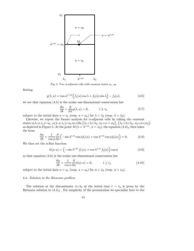
Fig. 5. Two φ-adjacent cells with constant states uL, uR
Setting
g(λ, u) = tanφe′,m(f1(u) cosλ+ f2(u) sinλ
)− f3(u), (4.6)
we see that equation (4.5) is the scalar one-dimensional conservation law
∂u
∂t+
∂
∂λg(λ, u) = 0, t ≥ tn (4.7)
subject to the initial data u = uL (resp. u = uR) for λ < λ2 (resp. λ > λ2).Likewise, we repeat the former analysis for φ-adjacent cells by taking the constant
states u(λ, φ, tn)=uL, u(λ, φ, tn)=uR in cells{λ1<λ<λ2, φ1<φ < φ2
},{λ1<λ<λ2, φ2<φ<φ3
},
as depicted in Figure 5. At the pointM(λ = λe,m, φ = φ2), the equation (4.4)φ then takesthe form
∂u
∂t+
1
cosφ
∂
∂φ
(− sinλe,m cosφf1(u) + cosλe,m cosφf2(u)
)= 0. (4.8)
We then set the φ-flux function
k(φ, u) =(− sinλe,m f1(u) + cosλe,m f2(u)
)cosφ (4.9)
so that equation (4.8) is the scalar one-dimensional conservation law
∂u
∂t+
1
cosφ
∂
∂φk(φ, u) = 0, t ≥ tn (4.10)
subject to the initial data u = uL (resp. u = uR) for φ < φ2 (resp. φ > φ2).
4.4. Solution to the Riemann problem
The solution at the discontinuity λ=λ2 at the initial time t = tn is given by theRiemann solution to (4.4)λ . For simplicity of the presentation we specialize here to the
14

flux (4.7). Since the dependence of g(λ, u) on λ is smooth, this solution is obtained byfixing λ = λ2, thus solving the classical conservation law
∂u
∂t+
∂
∂λg(λ2, u) = 0, t ≥ tn (4.11)
subject to the initial jump discontinuity of u.Here “e = 2” so that λe,m = λ2,m = λ2, etc.
We denote this solution by u2,m. Observe that the flux g(λ, u) in (4.11) is in gen-eral non-convex. The Riemann solution may therefore consist of several waves. It is aself-similar solution depending only on the slope (λ − λ2)/(t − tn). The value u2,m isthe value along the line λ=λ2. It therefore corresponds either to a sonic wave, namelyg′(λ2, u
2,m)=0, or to an “upwind value” u=uL (resp. u=uR) in the case where all wavespropagate to the right (resp. left).
Actually, the procedure for solving the Riemann problem in the case of a nonconvexflux function g(λ2, u) is well-known and goes back to classical works by Oleinik andothers. We recall it here briefly. Assume first that uL<uR. Consider the convex envelopeof g, namely, the largest convex continuous function gc, over the interval [uL, uR], suchthat gc≤g at all points. Clearly, gc=g in “convex sections” of the graph of g, while itconsists of linear segments when gc<g. It is easy to see that the “convex segments”,where g=gc, represent rarefaction waves (in the full Riemann solution) while the linearsegments represent jumps (i.e., shock waves). In particular, the solution u2,m is given bythe following formula:
u2,m = vmin, where g(λ2, vmin) ≤ g(λ2, v) for all v ∈ [uL, uR]. (4.12)
There are in fact three possibilities for this solution:a) uL < u2,m < uR, which implies that g′(λ2, u
2,m) = 0 (a sonic point).b) u2,m = uL, the whole wave pattern moves to the right.c) u2,m = uR, the whole wave pattern moves to the left.
Similarly, in the case uL>uR, we construct the “concave envelope” of g, namely, thesmallest concave continuous function gc such that gc≥g. Again the linear segments cor-respond to jump discontinuities while the concave segments (g=gc) correspond to rar-efaction waves. The solution to the Riemann problem is now given by u2,m=vmax, whereg(λ2, vmax)≥g(λ2, v), v ∈ [uR, uL]. As above, there are three possibilities for the solution(sonic, left-upwind, or right-upwind).
Replacing in the foregoing analysis the λ-flux function g(λ2, u) by the φ-flux functionk(φ2, u), the equation (4.10) reads
∂u
∂t+
∂
∂φ
(− sinλ2,mf1(u) + cosλ2,mf2(u)
)= 0, t ≥ tn . (4.13)
We get the Riemann solution to (4.13) in the three cases a), b), c) as above.
4.5. Convergence proof
The computational elements (“grid cells”) are denoted in [2] by K. Their sides aredenoted by e and the flux function across e is given by fe,K(u, v), where u is the (constant)value in K and v is the value in the neighboring cell (sharing the same side e) Ke. In
15

our grid of the sphere, some cells are actually pentagons; these are the cells whose lower-latitude side (along a latitude φ = const) borders the two higher-latitude sides of the twolower-latitude neighbor cells, as shown in Figure 3 for the southern hemisphere grid. Forsuch cells, the lower-latitude side consists of two faces, each one of them common withone of the lower-latitude neighboring cells.
With this construction of the grid, we can check the conditions in [2] imposed on thenumerical flux. It is important to keep in mind that we are dealing with the gradient fluxvectors given by Claim 2.2.
Claim 4.3 (Convergence of the proposed scheme.) Consider the first-order finitevolume scheme described above. Assume that the flux vector has the gradient form inClaim 2.2. Let fe,R(u, v) be the numerical flux calculated on the side e of the computa-tional cell R, using (4.3), where the midpoint value of u is obtained from the Riemannsolution. Then fe,R(u, v) satisfies the assumptions (5.5)-(5.7) of [2], and the numericalsolution converges to the exact solution as the maximal size of the grid cells shrinks tozero.
Proof. Consider the flux across a longitude side e : λ = λ2, which is given by Fλ inthe equation (4.4)λ . The procedure for integrating the flux across e is described by(4.3), while in Subsection 4.4 the calculation of Fλ(λ2, φ
2,m, u2,m) is described. It can besummarized as follows.
First, the solution u2,m to the Riemann problem associated with equation (4.4)λ isfound, assuming u, v to be the values on the two sides. However, note that Fλ dependsexplicitly on φ, and to be precise we need to replace in (4.4)λ the mean value φ2,m by φ.Thus, we find u2,m = u2,m(φ).
Clearly, in the case u = v we get identically u2,m(φ) = u = v and so the exact fluxsatisfies
Fλ = Fλ(λ2, φ, u2,m)
and its integration will give exactly the approximate value
fe,K(u, v) = −(h(e2, u2,m) − h(e1, u2,m)
),
as in (4.3). Thus, condition (5.5) in [2] is satisfied.Clearly, the conservation property (5.6) is satisfied even with the approximate defini-
tion.Also, the flux as defined in (4.3) makes it easy to check (5.7), as the flux is independent
of φ and the monotonicity is thus a result of general properties of the Riemann solver(even for nonconvex fluxes). For example, if u < v, one considers the convex envelope ofFλ, as defined in (4.4)λ (with φ = φ2,m) and then considers u2,m as the minimal valueon this envelope (over [u, v]). Clearly changing u upward will either change u2,m upwardor leave it unchanged. This completes the proof. 2
Remark 4.4 The convergence proof relies on the fact that the flux function is geometry-compatible. An inspection of the scheme shows that it can be applied also to fluxes that donot satisfy this condition. However, the quality of the numerical results (and indeed, alsosome features of the theoretical solution) are not known in this case. In all the numericalexamples in the present paper (Section 6) we use geometry-compatible fluxes.
16

5. Second-order extension based on the GRP solver
To improve the expected order of accuracy, we consider again the cell λ1<λ<λ2, φ1<φ<φ2
and assume that u is linearly distributed there. We use uL,λ, uL,φ (resp. uR,λ, uR,φ) to de-note the slopes in the cell to the left (resp. right) of the side λ=λ2. We also denote byuL(φ) (resp. uR(φ)) the limiting value (linearly distributed) of u at λ=λ2− (resp. λ=λ2+).Clearly, the solution to the Riemann problem across the discontinuity is a function ofφ, and we denote it by u2,m(φ), which conforms to our notation in Subsecion 4.4 above(where u was constant on either side of the discontinuity). The value of u2,m(φ) is ob-tained by solving the Riemann problem associated with Eq. (4.4)λ with φ2,m replaced byφ, subject to the initial data uL(φ), uR(φ). Restricting to the middle point φ = φ2,m, thesolution u2,m(φ2,m) (at λ = λ2,m = λ2) is in one of the three categories listed above (i.e.,sonic, left-upwind, right-upwind). By continuity, the solution u2,m(φ) will still be in thesame category for φ− φ2,m sufficiently small. The solution at (λ2,m, φ2,m) varies in timeand the GRP method deals with the determination of its time-derivative at that point.
Accounting for the variation of the solution over a time interval enables us to modifythe Godunov approach to the determination of edge fluxes, as presented in Section 4.3.We assume that the flux vector depends explicitly on x, as in (2.1). In what follows weuse for simplicity the “imbedded” notation x = (x1, x2, x3) for a point on the sphere (seethe Introduction), along with the corresponding spherical coordinates λ, φ. We furtherassume that the vector field Φ is given by the following extension of (2.3)
Φ(x, u) = ∇xh(x, u)
= q1(x1)f1(u) i1 + q2(x2)f2(u) i2 + q3(x3)f3(u) i3.(5.1)
The zero-divergence identity is obtained as a result of expressing Φ as a gradient ∇h inthe sense of Claim 2.2.
For our choice of Φ, such a representation of Φ as gradient of h is obtained when h istaken as
h(x, u) = r1(x1)f1(u) + r2(x2)f2(u) + r3(x3)f3(u) , (5.2)
and qj(xj) = r′j(xj), j = 1, 2, 3 .Using (1.2),(2.4) together with the geometry-compatibility property, we get an explicit
form of the conservation law (1.3) in our case as
∂u
∂t− sinλq1(x1)
∂
∂φf1(u) + cosλq2(x2)
∂
∂φf2(u)
+ tanφ(
cosλq1(x1)∂
∂λf1(u) + sinλq2(x2)
∂
∂λf2(u)
)− q3(x3)
∂
∂λf3(u) = 0.
(5.3)
Our GRP numerical approximation to this equation is based on an operator splittingapproach, by which we mean that the derivatives with respect to φ and λ are separatelyconsidered. We note that this approach has already been implemented in the Godunovcase (4.4). In that case, no use has been made of the geometry-compatibility property.Indeed, this has no bearing on the first-order scheme since the solution to the Riemannproblem is obtained by “freezing” the explicit dependence on λ, φ (and, in particular,ignoring the terms involving the derivatives with respect to this explicit dependence).In order to construct out second-order GRP scheme we proceed as follows.
17

The “λ-split” equation obtained from (5.3), is rewritten as an equation with a sourceterm (a balance law)
∂u
∂t+
∂
∂λg(x, u) = Sλ , t > tn
Sλ = tanφ2,m(f1(u)
∂
∂λ
(q1(x1) cosλ
)+ f2(u)
∂
∂λ
(q2(x2) sinλ
))− f3(u)
∂
∂λq3(x3),
g(x, u) = tanφ2,m(q1(x1) cosλf1(u) + q2(x2) sinλf2(u)
)− q3(x3)f3(u),
(5.4)
subject to the initial data (for u and its λ–slope) uL(φ2,m), uL,λ (resp. uR(φ2,m), uR,λ) forλ < λ2 (resp. λ > λ2). Observe that the equation is written in a “quasi-conservativeform”, which offers more convenience in the GRP treatment [3, Chap. 5]. The right-handside term Sλ is just the result of the (explicit) λ differentiation of the flux g(x, u). Thesolution u2,m to the associated Riemann problem is obtained by considering the limitingvalues uL(φ2,m), uR(φ2,m), as in Subsection 4.4.
Since the GRP approximation to the solution is given by
u2,m(φ2,m) +∂u
∂t(λ2,m, φ2,m, tn+)
∆t
2, ∆t = tn+1 − tn,
we need to determine the instantaneous time-derivative ∂u∂t
(λ2,m, φ2,m, tn+). This deriva-tive is given, in view of (5.4), by
∂u
∂t(λ2,m, φ2,m, tn+) = −um,λ
∂
∂ug(x, u)|λ2,m,φ2,m,u2,m ,
where the slope value um,λ is obtained by “upwinding”, determined by the associatedRiemann problem as follows.
i) u2,m = uL(φ2,m). (the wave moves to the right) and we then set
um,λ = uL,λ.
ii) u2,m = uR(φ2,m). (the wave moves to the left) and we then set
um,λ = uR,λ.
It remains to consider the sonic case. As noted above (Subsection 4.4), it remains sonicin the neighborhood of φ2,m, so that we have there ∂
∂ug(x, u)|λ2,m,φ2,m,u2,m = 0. The
time-derivative of u reduces therefore to
∂
∂tu(λ2,m, φ2,m, t=tn+) = 0.
The “φ-split” equation obtained from (5.3), is treated in analogy with the “λ-split”procedure outlined above.
In summary, the full equation (5.3) is resolved in two steps, i.e., the “λ–split” Equa-tion (5.4) and its “φ–split” analogue. Since these two equations refer to two differentmidpoints (i.e., the midpoint of λ = λ2 and the midpoint of φ = φ2), we cannot ex-pect, in general, the identical vanishing of the sum Sλ + Sφ. However, remark that thegeometry-compatibility condition (2.2) refers to the case of constant value of u. In thecase at hand, setting u ≡ u constant in the computational cell and its neighbors implies
18

the vanishing of all slopes, and hence the vanishing of all instantaneous time-derivativesof the solution to the GRP at all midpoints of the cell interfaces. The solution thereforeremains constant u = u. This is the sense in which the geometry-compatibility conditionis satisfied in the GRP framework.
6. Numerical tests
6.1. First test case: equatorial periodic solutions
Here, the conservation law takes the form (3.1) and the flux function and initial dataare given by
f1(u) = f2(u) = 0, f3(u) = −2π (u2/2),
u(λ, φ, 0) =
{sinλ, 0 < λ < 2π, 0 < φ < π/12,
0, otherwise.
(6.1)
As discussed in Section 3 (see the discussion of solutions to (3.1)) it is clear that thesolution here (as a function of λ) is identical to the periodic solution for the Burgersequation in R
1, with periodic boundary conditions on [0 < x < 2π]. However, we computethe numerical solution here on our spherical grid, and we need to check not only thatit conforms with the one-dimensional case but that it does not “leak” beyond the bandsupporting the initial data. The results at the shock formation time ts = 1/2π are shownin Figure 6 for ∆λ = 2π/16, in Figure 7 for ∆λ = 2π/32 and in Figure 8 for ∆λ = 2π/64.These GRP solutions to (4.7) clearly converge to the exact solution with refinement ofthe λ grid, and are comparable to the corresponding solution to the scalar conservationlaw in R
1 with ∆x = 2π/22.
-1.0
-0.8
-0.6
-0.4
-0.2
0.0
0.2
0.4
0.6
0.8
1.0
0.0 0.1 0.2 0.3 0.4 0.5 0.6 0.7 0.8 0.9 1.0
GRP/SCL GRP/SPHERE
Exact
x = λ/2π
u
Fig. 6. Exact, GRP/SCL and GRP/SPHERE (∆λ=2π/16) solutions to the IVP (6.1) at t = 1/2π
19

-1.0
-0.8
-0.6
-0.4
-0.2
0.0
0.2
0.4
0.6
0.8
1.0
0.0 0.1 0.2 0.3 0.4 0.5 0.6 0.7 0.8 0.9 1.0
GRP/SCL GRP/SPHERE
Exact
x = λ/2πu
Fig. 7. Exact, GRP/SCL and GRP/SPHERE (∆λ=2π/32) solutions to the IVP (6.1) at t = 1/2π
-1.0
-0.8
-0.6
-0.4
-0.2
0.0
0.2
0.4
0.6
0.8
1.0
0.0 0.1 0.2 0.3 0.4 0.5 0.6 0.7 0.8 0.9 1.0
GRP/SCL GRP/SPHERE
Exact
x = λ/2π
u
Fig. 8. Exact, GRP/SCL and GRP/SPHERE (∆λ=2π/64) solutions to the IVP (6.1) at t = 1/2π
6.2. Second test case: steady state solution
We refer to Corollary 3.3 and using the notation there we take the flux vector andinitial data as:
f1(u) = u2/2, f2(u) = f3(u) = 0,
u(λ, φ, 0) = cosλ cosφ.(6.2)
Using the terminology of Corollary 3.3 we see that the initial function is the “simplest”possible function, corresponding to g(x1) = x1.
As is shown in Figure 9, the numerical solution remains nearly unchanged in timeafter being subjected to integration up to t = 6 by the GRP scheme with constant timestep ∆t = 0.04, the (color) maps of u(λ, φ, t) at the initial and final times are virtuallyindistinguishable. The shown grid has latitude step ∆φ = π/60, and an equatoriallongitude step ∆λ = π/64. A measure udiff of the numerical solution error is defined
20

-1-.8-.6-.4-.2 0 .2 .4 .6 .8 1
Fig. 9. Steady-state initial data (and solution) to the IVP (6.2) at t = 6.Color map range scaled to (umin, umax) = (−0.998, 0.998).
as the l1–norm difference |u(λ, φ, 6) − u(λ, φ, 0)|, obtained by summation over all gridcells. In this case we obtained udiff = 0.0083, which is small relative to the full rangeumax − umin = 2. We also calculated the stability ratio, defined as
µCF L = max {∆tw/Lcell} ,where w, Lcell are the wave speed and the cell length in either coordinate direction,respectively. The maximum value is taken over all cells and all time-integration steps. Inthe present case we obtained µCF L = 0.55. This test case demonstrates that the GRPscheme correctly computes the time-evolution for the non-constant data (6.2), whichidentically vanishes for the exact (steady) solution.
6.3. Third test case: steady state solution in a spherical cap
Referring to Remark 3.6 we construct a conservation law having a steady solution asfollows. The flux vector and initial data are:
f1(u) = f2(u) = f3(u) = u2/2,
u(λ, φ, 0) = (x1 + x2 + x3)/√
3 = [cosφ(cosλ+ sinλ) + sinφ]/√
3,(6.3)
As is shown in Figure 10, the numerical solution remains nearly unchanged in timeafter being subjected to integration up to t = 6 by the GRP scheme with constant time
21

-1-.8-.6-.4-.2 0 .2 .4 .6 .8 1
Fig. 10. Steady-state initial data (and solution) to the IVP (6.3) at t = 6.Color map range scaled to (umin, umax) = (−0.998, 0.998).
step ∆t = 0.015, the color maps of u(λ, φ, t) at the initial and final times are virtuallyindistinguishable. The shown grid has latitude step ∆φ = π/60, and an equatoriallongitude step ∆λ = π/64. Again, the l1–norm of the difference is udiff = 0.013, whichis small relative to the full range umax − umin = 2. The stability ratio obtained inthe present case is µCF L = 0.60. This test case provides a second example of an accuratecalculation of a steady state. Unlike the previous example, the level curves of the solutionare transversal to the coordinate directions.
6.4. Fourth test case: confined solutions
We take (as in Claim 2.2) Φ(x, u) = ∇h(x, u), where h(x, u) = ψ(x1)x1f1(u). Thefunction ψ(x1) is defined by
ψ(x1) =
1, x1 ≤ 0,
1 − 6x21 +
8√2x3
1, 0 ≤ x1 ≤√
2
2,
0,
√2
2≤ x1 .
(6.4)
The flux vector is then given by
F(x, u) = n(x) × Φ(x, u).
22

The solution is clearly confined to the sector x1 ≤√
2
2of the sphere. Its boundary is a
circle which intersects the meridian λ = 0 at φ = π4.
The flux in the subdomain x1 ≤ 0 is given by
F(x, u) = n(x) × f1(u) i1,
so if we take the initial data as ψ(x1)u0(x1), where u0 is the steady state solution ofthe second test case (and also the same f1(u)), the solution remains steady in that part,
namely, in x1 ≤ 0. Clearly, it evolves in time in the region 0 ≤ x1 ≤√
2
2, but vanishes
identically (for all time) if√
2
2≤ x1.
The confined IVP was integrated in time up to t = 6 by the GRP scheme, using thesame grid and time step as in the second test case (Subsection 6.2). The solution isrepresented by the color map in Figure 11. It shows clearly that the solution remainsconfined to the cap x1 <
√1/2 . The stability ratio obtained in the present case, with
constant integration time step ∆t = 0.04, is µCF L = 0.55.
-1-.8-.6-.4-.2 0 .2 .4 .6 .8 1
Fig. 11. Confined solution test case, with the IVP data to the IVP (6.4) at t = 6.Color map range scaled to (umin, umax) = (−0.998, 0.183).
6.5. Fifth test case: The Williamson test case #1
This test case is the first of seven test cases suggested by Williamson et al. [14],specifically for the shallow water equations that model the global air flow on the rotatingearth. In this case the earth rotation is set to zero, and a ”cosine bell” patch of thelevel function h(λ, φ, t) is advected by a constant-magnitude wind along a great circle
23

oriented at an angle α relative to the polar axis. The shallow water system reducesin this case to the scalar conservation law (1.3), where the scalar function is the levelfunction h(λ, φ, t) = u(λ, φ, t). In particular, the corresponding flux function is found tobe geometry compatible. Translated to our framework, this test case is as follows. Theinitial function is given by
u(λ, φ, 0) =
{(H0/2)[1 + cos(πρ/R)], ρ < R,
0, ρ ≥ R ,(6.5)
where (for the unit sphere) R = 1/3, and the (normalized) peak level is taken as H0 = 1.The angle ρ is given by
ρ = arccos[sinφc sinφ+ cosφc cosφ cos(λ− λc)] .
where the center of the cosine bell is taken as
[λc, φc] = [0.5π, 0] .
The flux vector is linear in u and is given by
Fλ(λ, φ, u) = V0u[cosφ cosα+ sinφ cosλ sinα],
Fφ(λ, φ, u) = −V0u sinλ sinα .
The constant V0 represents the magnitude of the velocity in the original setup of thistest case [14], and it is given by V0 = 2π/tf for a complete trajectory around the sphereat time tf . In the numerical example we took tf = 12, and a constant time step ∆t =0.008. The l1–error measure at the final time was udiff = 0.05 and the CFL coefficientµCFL = 0.43. Compared to the l1 measure of the initial cosine-bell function of about0.30, this represents a relative error of 1/6.
The initial setup (t = 0) is shown in Figure 12 and the final map is shown in Figure 13.The great circle trajectory is also shown in these plots (note that it reaches a peak latitudeangle of φ = π/2 − α = π/2 − 0.05, near the pole). The shown grid has latitude step∆φ = π/126, and an equatorial longitude step ∆λ = π/128. The CPU time on a PCwith Pentium IV processor was 140 seconds (all former examples took considerably lesstime).
Comparing the initial and final color maps, we note a very good preservation of theround bell-shape – noting only slight widening and distortion at the final time. The peakvalue, though, was smeared out: It decreased from the initial value of 0.991 to the finalvalue of 0.833, i.e., about 16% drop, which is comparable to the previously mentionedrelative value of the l1-error. Note that the initial peak value is lower than the exact levelof H0 = 1 due to averaging of initial data in cells. This error is quite small, consideringthat the initial patch radius is resolved by just about 14 grid cells.
The present test case demonstrates that the present GRP scheme shows promise toperform well when adapted to the shallow water system.
7. Summary and Discussion
The numerical treatment of the shallow-water equations on the sphere has been ad-dressed in a large number of works. We refer to [7]–[13] and references therein. However,
24

-1-.8-.6-.4-.2 0 .2 .4 .6 .8 1
Fig. 12. The Williamson test case #1. Trajectory: α = 0.05. to the IVP (6.5) at the initial state t = 0.Color map range scaled to (umin, umax) = (0, 0.991).
unlike the scalar Burgers equation, which has served as a simplified model in the theo-retical and numerical studies of hyperbolic conservation laws in a Cartesian framework,there has been no such analogue in the spherical case. The present paper, a third in aseries (following the theoretical study [6] and the general finite volume framework [2]) ismeant to serve this purpose. The points that have been emphasized in this paper can besummarized as follows.
(a) We have seen a large wealth of flux functions which, combined with the geometricstructure, allow for a variety of analytic nontrivial solutions. Such solutions can bestationary or confined to pre-determined sectors on the sphere.
(b) The design of the finite volume scheme is strongly connected to the analytic propertiesof the equation, as well as to the underlying geometry. In particular, length and areameasurements of mesh cells are treated exactly, so that the “null-divergence” conditionis rigorously satisfied on the discrete level.
(c) The use of the GRP second-order methodology improves considerably the quality ofthe numerical solution.
25
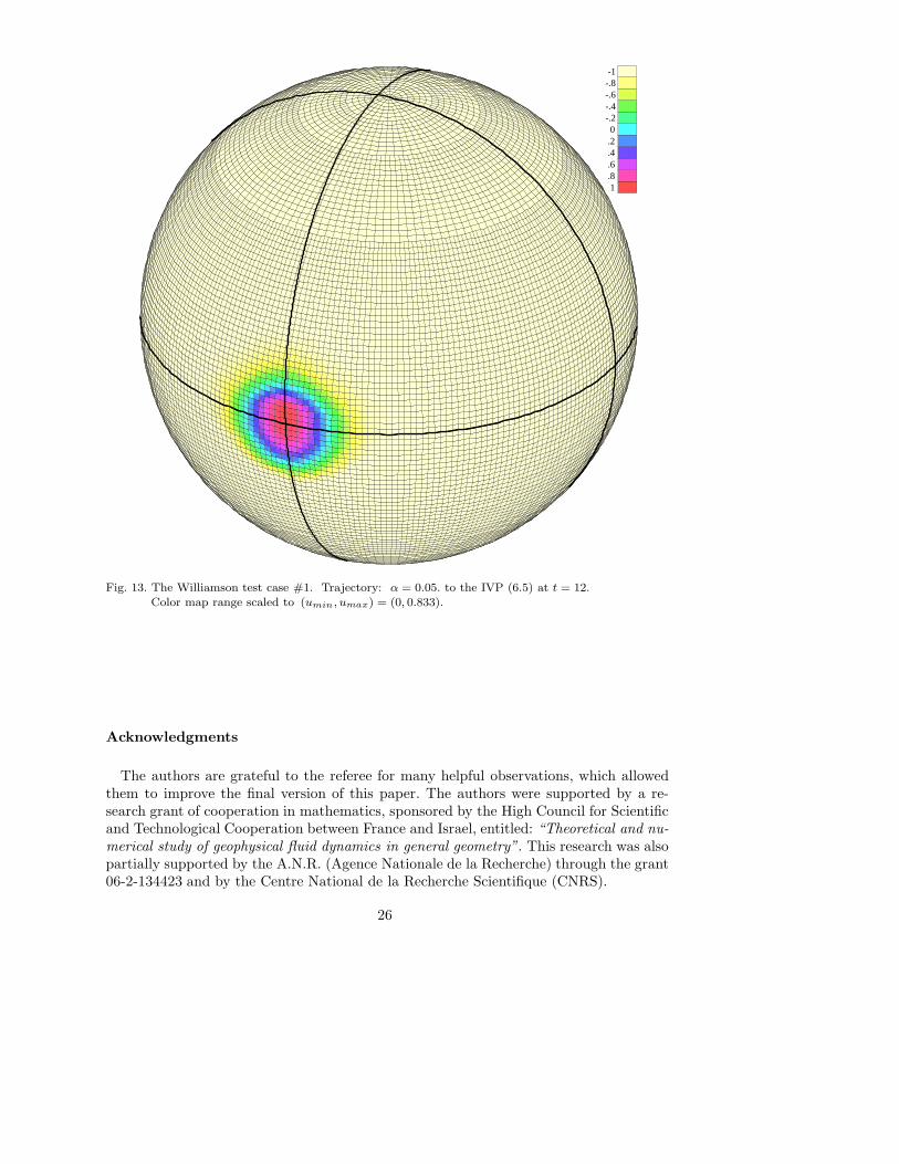
-1-.8-.6-.4-.2 0 .2 .4 .6 .8 1
Fig. 13. The Williamson test case #1. Trajectory: α = 0.05. to the IVP (6.5) at t = 12.Color map range scaled to (umin, umax) = (0, 0.833).
Acknowledgments
The authors are grateful to the referee for many helpful observations, which allowedthem to improve the final version of this paper. The authors were supported by a re-search grant of cooperation in mathematics, sponsored by the High Council for Scientificand Technological Cooperation between France and Israel, entitled: “Theoretical and nu-merical study of geophysical fluid dynamics in general geometry”. This research was alsopartially supported by the A.N.R. (Agence Nationale de la Recherche) through the grant06-2-134423 and by the Centre National de la Recherche Scientifique (CNRS).
26

References
[1] P. Amorim, P.G. LeFloch, and B. Okutmustur, Finite volume schemes on Lorentzian manifolds,Comm. Math. Sc. 6 (2008), 1059–1086.
[2] P. Amorim, M. Ben-Artzi, and P.G. LeFloch, Hyperbolic conservation laws on manifolds. Totalvariation estimates and the finite volume method, Meth. Appli. Analysis 12 (2005), 291–324.
[3] M. Ben-Artzi and J. Falcovitz, Generalized Riemann problems in computational fluid dynamics,
Cambridge University Press, London, 2003.
[4] M. Ben-Artzi, J. Falcovitz, and P.G. LeFloch, Hyperbolic conservation laws on the sphere. Theshallow water model, in preparation.
[5] M. Ben-Artzi, J. Falcovitz, and J. Li, Wave interactions and numerical approximation for two-dimensional scalar conservation laws, Comp. Fluid Dynamics J. 14 (2006), 401–418.
[6] M. Ben-Artzi and P.G. LeFloch, The well-posedness theory for geometry-compatible hyperbolicconservation laws on manifolds, Ann. Inst. H. Poincare : Nonlin. Anal. 24 (2007), 989–1008.
[7] F.X. Giraldo, Lagrange-Galerkin methods on spherical geodesic grids: The shallow water equations,J. Comput. Phys. 160 (2000), 336–338.
[8] G.J. Haltiner, Numerical weather prediction, John Wiley Press, 1971.
[9] P.G. LeFloch, Neves W., and B. Okutmustur, Hyperbolic conservation laws on manifolds. Errorestimate for finite volume schemes, Acta Math. Sinica (2009).
[10] J. Li, S. Yang, and T. Zhang, The two-dimensional Riemann problem in gas dynamics, PitmanPress, 1998.
[11] R. Nair and C. Jablonowski, Moving vortices on the sphere: A test case for horizontal advectionproblems, Month. Weather Rev. 136 (2008), 699–711.
[12] C. Ronchi, R. acono and P.S. Paolucci, The “Cubed Sphere””: A new method for the solution of
partial differential equations in spherical geometry, J. Comput. Phys. 124 (1996), 93–114.
[13] A. Rossmanith, A wave propagation method for hyperbolic systems on the sphere, J. Comput.Phys. 213 (2006), 629–658.
[14] D.L. Williamson, J.B. Drake, J.J. Hack, R. Jakob, and P.N. Swarztrauber, A standard test set fornumerical approximations to the shallow water equations in spherical geometry, J. Comput. Phys.102, (1992), 211–224.
27