HYPERCONGESTION

Kenneth A. Small and Xuehao Chu May 12, 2003 Forthcoming, Journal of Transport Economics and Policy JEL Codes: R41, H23, C61 Keywords: congestion, hypercongestion, externalities, peakload pricing, dynamic analysis, speed-flow

curves Addresses:

Prof. Kenneth A. Small* Dept. of Economics University of California Irvine, CA 92697-5100 tel: 949-824-5658 fax: 949-824-2182 e-mail: ksmall@uci.edu

Dr. Xuehao Chu Center for Urban Transportation Research University of South Florida Tampa, FL 33620 tel: 813-974-9831 fax: 813-974-5168 e-mail: xchu@cutr.eng.usf.edu

* Corresponding author Financial support from the U.S. Department of Transportation and the California Department of Transportation, through the University of California Transportation Center, is gratefully acknowledged. We thank Helen Wei for research assistance. We also thank Richard Arnott, John Bates, Fred Hall, Timothy Hau, John McDonald, Se-il Mun, Claude Penchina, Erik Verhoef, and anonymous referees for insightful discussions and comments on earlier drafts. However, the authors are solely responsible for all statements and opinions expressed.

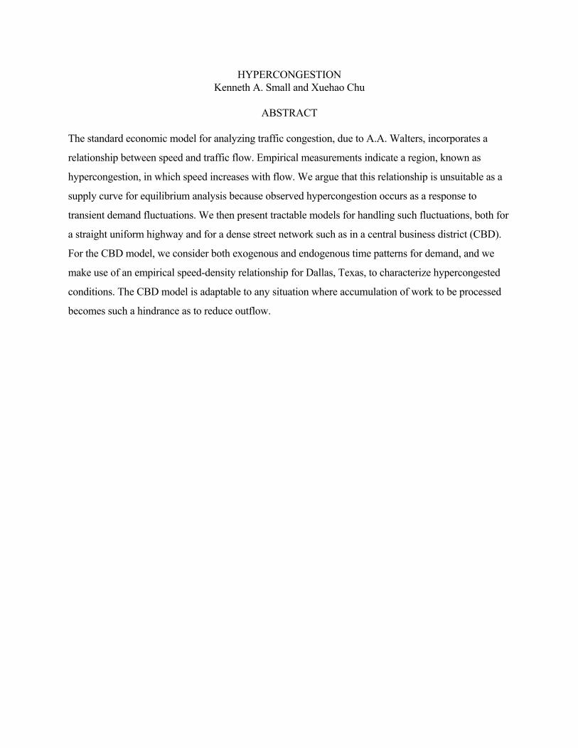
HYPERCONGESTION Kenneth A. Small and Xuehao Chu ABSTRACT The standard economic model for analyzing traffic congestion, due to A.A. Walters, incorporates a

relationship between speed and traffic flow. Empirical measurements indicate a region, known as

hypercongestion, in which speed increases with flow. We argue that this relationship is unsuitable as a

supply curve for equilibrium analysis because observed hypercongestion occurs as a response to

transient demand fluctuations. We then present tractable models for handling such fluctuations, both for

a straight uniform highway and for a dense street network such as in a central business district (CBD).

For the CBD model, we consider both exogenous and endogenous time patterns for demand, and we

make use of an empirical speed-density relationship for Dallas, Texas, to characterize hypercongested

conditions. The CBD model is adaptable to any situation where accumulation of work to be processed

becomes such a hindrance as to reduce outflow.

1

HYPERCONGESTION

Kenneth A. Small and Xuehao Chu

Introduction

It has been more than a third of a century since A.A. Walters (1961) established what is now the

standard way economists think about congestion, using the engineering relationship between travel time

on a given length of highway and the traffic flow rate.1 Walters noted that by identifying flow as

quantity, the engineering relationship could be viewed as an average cost curve (with a suitable

transformation from travel time to cost) and then combined with a demand curve to analyze equilibria

and optima. Optima can be achieved via a Pigovian charge known as a congestion toll. This model has

proved extraordinarily fruitful in the study of transportation, other congestible facilities such as

telephone service, Internet traffic, and electricity transmission, and even more widely in the literature on

local public finance and clubs.2

One feature, however, gave Walters some difficulty and has caused endless trouble ever since.

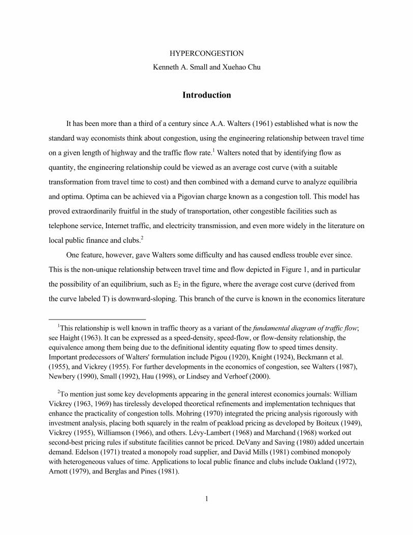
This is the non-unique relationship between travel time and flow depicted in Figure 1, and in particular

the possibility of an equilibrium, such as E2 in the figure, where the average cost curve (derived from

the curve labeled T) is downward-sloping. This branch of the curve is known in the economics literature

1This relationship is well known in traffic theory as a variant of the fundamental diagram of traffic flow; see Haight (1963). It can be expressed as a speed-density, speed-flow, or flow-density relationship, the equivalence among them being due to the definitional identity equating flow to speed times density. Important predecessors of Walters' formulation include Pigou (1920), Knight (1924), Beckmann et al. (1955), and Vickrey (1955). For further developments in the economics of congestion, see Walters (1987), Newbery (1990), Small (1992), Hau (1998), or Lindsey and Verhoef (2000).

2To mention just some key developments appearing in the general interest economics journals: William Vickrey (1963, 1969) has tirelessly developed theoretical refinements and implementation techniques that enhance the practicality of congestion tolls. Mohring (1970) integrated the pricing analysis rigorously with investment analysis, placing both squarely in the realm of peakload pricing as developed by Boiteux (1949), Vickrey (1955), Williamson (1966), and others. Lévy-Lambert (1968) and Marchand (1968) worked out second-best pricing rules if substitute facilities cannot be priced. DeVany and Saving (1980) added uncertain demand. Edelson (1971) treated a monopoly road supplier, and David Mills (1981) combined monopoly with heterogeneous values of time. Applications to local public finance and clubs include Oakland (1972), Arnott (1979), and Berglas and Pines (1981).

2

as the region of "hypercongestion," in contrast to the lower branch which depicts a condition we will

call “ordinary congestion.”3 Walters described equilibrium E2 as "The Bottleneck Case" (p. 679), a

terminology which is not fully explained but which, as we shall see, is highly appropriate in the case of

a straight road.

The conventional interpretation of E2, encouraged if not specifically stated by Walters, is that it is

just an especially inefficient equilibrium. It follows that first-order welfare gains are possible by

somehow shifting the equilibrium down to the lower branch of the curve. Serious arguments about

Pareto-improving tolls have been based on just this argument, both for highways (Johnson 1964) and by

analogy for renewable resources (De Meza and Gould 1987).

But this view has problems. For one thing, E2 is not obviously a stable equilibrium (Newbery

1990, p. 28). Consider a simple quantity-adjustment mechanism on the demand side in response to a

small upward fluctuation ∆T in travel time, due for example to an influx of inexperienced drivers.

3Engineering terminology sometimes differs, with the upper branch called "congested” or “oversaturated" flow and the lower branch called "uncongested," “undersaturated,” or "free” flow. We use the terminology most common in the economics literature.

Figure 1A Model of Travel Time Versus Flow

Flow (q )

Trav

el ti

me

per m

ile ( T

)

T

D1

D2

E1

E2

∆T∆q

3

Quantity demanded would be reduced by ∆q in Figure 1; according to the hypercongested "supply"

curve, this in turn would cause a further increase in travel time; and so forth. This is shown in the

figure. We could try instead making curve D2 steeper, so as to cut T from above. Or we could define

other dynamic adjustment mechanisms. But as Verhoef (1999) shows, none of these devices produces

stable hypercongested equilibria.4

Even aside from stability, it is economically illogical to treat the AC curve in the neighborhood of

E2 as a supply curve. To do so suggests that a smaller quantity demanded makes traffic worse, so that

drivers confer a positive externality on each other.5

The underlying problem is that although Figure 1 purports to portray the simultaneous behavior of

demand and supply curves, in fact the quantities (vehicle flows) that logically enter the demand and

supply analyses are not the same things—a point hinted at by Walters, made clearly by Neuburger

(1971), and reiterated by many subsequent authors.6 Roughly speaking, quantity demanded is

represented by inflow and quantity supplied by outflow. But inflow and outflow on a road segment

often differ. When they do, vehicle density cannot be uniform along the road, and the engineering

4More precisely, Verhoef (1999,p. 349) shows that equilibria on the upper branch of Figure 1 cannot be stable with respect to both price and quantity perturbations. He also shows that there is no plausible dynamic process that could lead from an equilibrium like E1 to an equilibrium on the upper branch. Verhoef’s conceptual argument is further buttressed by a specific dynamic car-following model in Verhoef (2001).

5One can construct network paradoxes where increasing the quantity demanded in one place can improve travel times elsewhere (Fisk 1979). However, such cases are not described by a simple supply curve. Other authors have similarly concluded that a properly defined supply curve must be rising (Hills 1993, Yang and Huang 1998). 6See May, Shepherd, and Bates (2000) for an illuminating discussion. Walters referred to the backward-bending portion of curve AC as "the equilibrium relation between flow and unit cost when density has been taken into account" (p. 680), but his explanation is clumsy at best. Hills (1993) notes that "demand should be measured in terms of the number of vehicles wishing to embark on trips during a given period of time" (p. 96). McDonald and d'Ouville (1988) make a similar distinction between inflow and outflow by defining them as inputs and outputs, respectively, of a production function. Else (1981), Alan Evans (1992), and Ohta (2001) try to rescue the static analysis by redefining quantity demanded as density. Evans rejects a curve like D1 in Figure 1 as a valid demand curve because "consumers do not choose the traffic flow given the price" (p. 212). But consumers do not choose density either; rather, density is a stock variable which depends on past inflows and on capacity and other parameters of the flow-density relationship, so is not a suitable measure of quantity demanded. A more helpful way of viewing the matter is the distinction between a “performance curve,” which describes variables measured over a specified range of places and times, and a “supply curve,” which describes variables encountered by a given vehicle. This distinction can be extended to a network, as described by May et al. (2000).

4

relationship underlying curve AC in Figure 1 no longer applies. Instead, an explicitly dynamic theory is

required, such as the "kinematic" theory of Lighthill and Whitham (1955) or a car-following theory

based on micro driver behavior (Herman 1982, Verhoef 2001). These theories explain, for example, the

stop-and-go conditions so familiar to expressway drivers.

Dynamic phenomena are especially crucial when demand is changing rapidly. In practice,

congestion on roads and most other facilities is a peak-load phenomenon. For ordinary congestion,

ignoring the peaked character of demand might be an adequate approximation.7 But for

hypercongestion, peaking is the whole game. As stated succinctly by Arnott (1990, p. 200):

"hypercongestion occurs as a transient response of a non-linear system to a demand spike."

This paper proposes ways to deal with such demand spikes. The same approach could equally

well handle transient reductions in capacity. In the sections that follow, we demonstrate more fully the

truth of Arnott's characterization of hypercongestion. We then develop the consequences for two quite

different situations: a uniform stretch of roadway, and a dense street network. Our goal is to provide

tractable models for economic analysis, so we make some simplifications compared to a fully

developed engineering model of traffic flow. We also ignore randomness in demand and capacity.

In the case of a uniform expressway, our simplification leads to a piecewise-linear average cost

function based on simple queuing theory. Hypercongestion occurs but is irrelevant because its

characteristics affect only the flow inside the queue, not total trip times.

In the case of a dense street network, we suggest two alternate simplifications, each of which

allows hypercongestion to occur and to create large costs. These models are applicable to many

situations where congestion degrades throughput. Telephone networks may break down when switching

equipment is overtaxed. Storm drains clog when high water flow carries extra debris. Bureaucrats are

distracted by extra inquiries when an unusually high flow of paperwork causes them to get behind. All

these situations can lead either to temporary problems (busy signals, moderate flooding) or to a

complete breakdown known as gridlock. Our model produces these features in a plausible and tractable

way.

7An example is Agnew (1977), who formulates a model akin to one of ours but considers only permanent changes in demand. Although his model does produce hypercongested equilibria, with all the inconsistencies we have described, those equilibria are only temporary so do not have much effect on the questions he considers.

5

Queuing Makes the Supply Curve Upward-Sloping

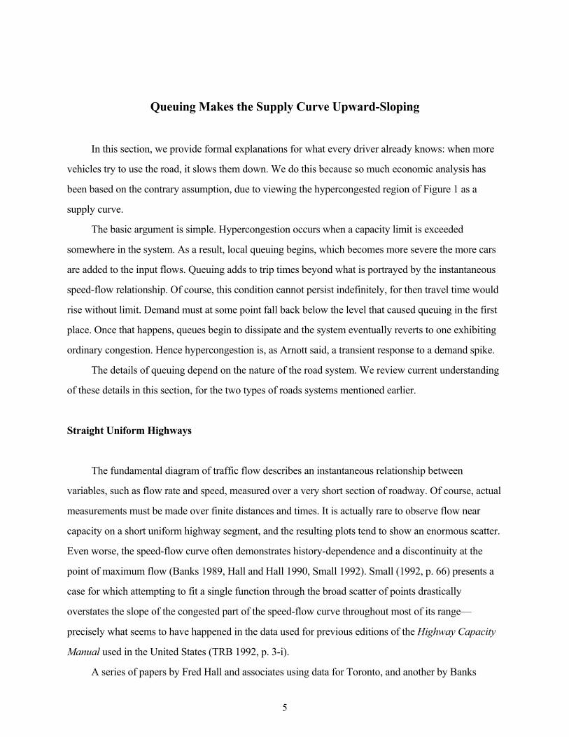
In this section, we provide formal explanations for what every driver already knows: when more

vehicles try to use the road, it slows them down. We do this because so much economic analysis has

been based on the contrary assumption, due to viewing the hypercongested region of Figure 1 as a

supply curve.

The basic argument is simple. Hypercongestion occurs when a capacity limit is exceeded

somewhere in the system. As a result, local queuing begins, which becomes more severe the more cars

are added to the input flows. Queuing adds to trip times beyond what is portrayed by the instantaneous

speed-flow relationship. Of course, this condition cannot persist indefinitely, for then travel time would

rise without limit. Demand must at some point fall back below the level that caused queuing in the first

place. Once that happens, queues begin to dissipate and the system eventually reverts to one exhibiting

ordinary congestion. Hence hypercongestion is, as Arnott said, a transient response to a demand spike.

The details of queuing depend on the nature of the road system. We review current understanding

of these details in this section, for the two types of roads systems mentioned earlier.

Straight Uniform Highways

The fundamental diagram of traffic flow describes an instantaneous relationship between

variables, such as flow rate and speed, measured over a very short section of roadway. Of course, actual

measurements must be made over finite distances and times. It is actually rare to observe flow near

capacity on a short uniform highway segment, and the resulting plots tend to show an enormous scatter.

Even worse, the speed-flow curve often demonstrates history-dependence and a discontinuity at the

point of maximum flow (Banks 1989, Hall and Hall 1990, Small 1992). Small (1992, p. 66) presents a

case for which attempting to fit a single function through the broad scatter of points drastically

overstates the slope of the congested part of the speed-flow curve throughout most of its range—

precisely what seems to have happened in the data used for previous editions of the Highway Capacity

Manual used in the United States (TRB 1992, p. 3-i).

A series of papers by Fred Hall and associates using data for Toronto, and another by Banks

6

(1989) using data for San Diego, have established the primary reason for these problems in the case of

urban expressways (Hall, Hurdle, and Banks 1992). Traffic that is in or near a condition of

hypercongestion is almost always influenced by a nearby bottleneck. Because of entrance ramps and

variations in the roadway, the ratio of flow to capacity is never constant across distance. Instead, local

bottlenecks occur where capacity is exceeded, and these affect adjacent sections: upstream of a

bottleneck traffic tends to form a queue, while downstream it is metered to a level well below the

capacity of that section. Within the queue, the speed-flow relationship is hypercongested but not

necessarily well-defined.8

The upshot, then, is that hypercongestion on an urban expressway usually occurs as part of a

queue. Where it occurs, the flow rate is governed not by quantity demanded but rather by downstream

bottleneck capacity. The density within this queue is irrelevant to total trip time; hence so is the nature

of the hypercongested speed-flow relationship. Rather, total trip time for a given vehicle is governed by

the total number of vehicles in front of it (up to the bottleneck) and the rate at which they can flow

through the bottleneck.

To demonstrate this statement, we follow Mun (1994, 2002) and consider the most common

queuing model, in which bottleneck capacity is independent of flow conditions in the queue.9 Let L be

8 Branston (1976) and Hall and Hall (1990) show that the relationship is sensitive to exactly how the bottleneck formed. Cassidy (1998) shows that the relationship is more predictable if attention is limited to observations for which speed is nearly constant within the time interval over which it is measured. There is a growing physics literature using micro-simulation to derive unexpected macro properties, including chaotic behavior, for traffic flow based on plausible micro behavior. See Helbing and Treiber (1998) for a review. Some of these papers have reported empirical observations of spontaneous transitions to apparently stable steady states involving hypercongestion (e.g. Kerner and Rihborn 1997). However, Daganzo, Cassidy and Bertini (1999) show that Kerner and Rehborn's observations are more simply explained as hypercongestion occurring in a queue, just as described here. McDonald, d’Ouville and Liu (1999) also describe purported observations of steady-state hypercongestion on Chicago expressways; however, it is extremely difficult to rule out the possibility that they are created by bottlenecks resulting from inhomogeneities in the roadway. Even an exit ramp can create a point of reduced capacity if slow traffic on the ramp causes drivers on the mainline lanes to slow down for caution, as shown by Muñoz and Daganzo (2002).

9All the "link capacity functions" reviewed by Branston (1976), and most models used in traffic micro-simulation, have this property. If, in contrast, the capacity of a bottleneck depends on upstream conditions or on the history of past flow conditions, then a more complex model such as by Neuberger (1971) or Yang and Huang (1997) is required. There is indeed evidence that the capacity of an expressway bottleneck sometimes drops by a few percent immediately after a queue forms behind it. Cassidy and Bertini (1999) review this evidence and add their own which shows a 4-10 percent drop (p. 39). However, they find that the high flow rates typically preceding the onset of queuing lack day-to-day

7

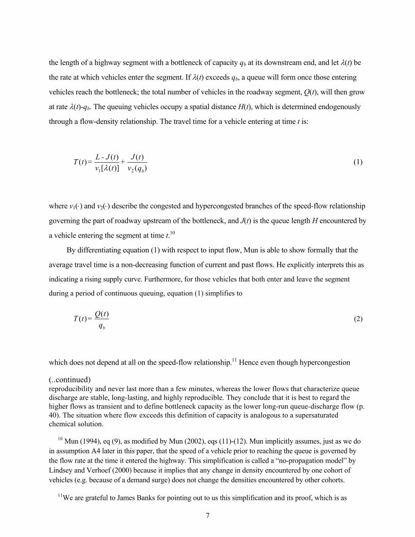
the length of a highway segment with a bottleneck of capacity qb at its downstream end, and let λ(t) be

the rate at which vehicles enter the segment. If λ(t) exceeds qb, a queue will form once those entering

vehicles reach the bottleneck; the total number of vehicles in the roadway segment, Q(t), will then grow

at rate λ(t)-qb. The queuing vehicles occupy a spatial distance H(t), which is determined endogenously

through a flow-density relationship. The travel time for a vehicle entering at time t is:

where v1(⋅) and v2(⋅) describe the congested and hypercongested branches of the speed-flow relationship

governing the part of roadway upstream of the bottleneck, and J(t) is the queue length H encountered by

a vehicle entering the segment at time t.10

By differentiating equation (1) with respect to input flow, Mun is able to show formally that the

average travel time is a non-decreasing function of current and past flows. He explicitly interprets this as

indicating a rising supply curve. Furthermore, for those vehicles that both enter and leave the segment

during a period of continuous queuing, equation (1) simplifies to

which does not depend at all on the speed-flow relationship.11 Hence even though hypercongestion

(..continued) reproducibility and never last more than a few minutes, whereas the lower flows that characterize queue discharge are stable, long-lasting, and highly reproducible. They conclude that it is best to regard the higher flows as transient and to define bottleneck capacity as the lower long-run queue-discharge flow (p. 40). The situation where flow exceeds this definition of capacity is analogous to a supersaturated chemical solution. 10 Mun (1994), eq (9), as modified by Mun (2002), eqs (11)-(12). Mun implicitly assumes, just as we do in assumption A4 later in this paper, that the speed of a vehicle prior to reaching the queue is governed by the flow rate at the time it entered the highway. This simplification is called a “no-propagation model” by Lindsey and Verhoef (2000) because it implies that any change in density encountered by one cohort of vehicles (e.g. because of a demand surge) does not change the densities encountered by other cohorts.

11We are grateful to James Banks for pointing out to us this simplification and its proof, which is as

)()(

)]([)()(

21 qvtJ +

tvtJ - L = tT

bλ (1)

qtQ = tT b

)()( (2)

8

exists, it is irrelevant to users who care only about total travel time.12

Dense Street Networks

The fundamental diagram of traffic flow is not expected to apply to an entire network of streets.

Instead, analysis typically proceeds by simulation using queuing theory at each intersection.13

Considerable work has been done trying to characterize the "oversaturation delay" in such a situation,

both for single intersections and for groups of intersections. One purpose of such work has been to

develop relationships between travel time and input-flow characteristics for use in intersection design,

as for example in the Highway Capacity Manual (TRB 1992, ch. 9). These relationships have the

property one expects from ordinary experience: greater inflows cause greater delays.

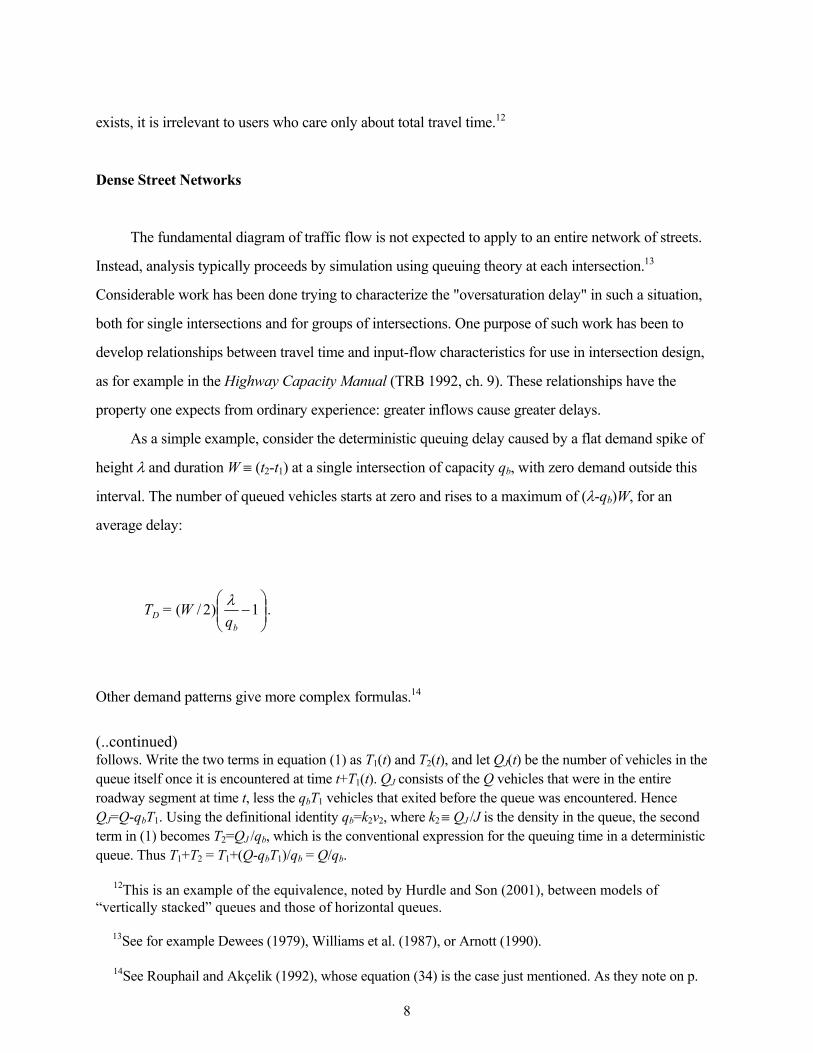
As a simple example, consider the deterministic queuing delay caused by a flat demand spike of

height λ and duration W ≡ (t2-t1) at a single intersection of capacity qb, with zero demand outside this

interval. The number of queued vehicles starts at zero and rises to a maximum of (λ-qb)W, for an

average delay:

Other demand patterns give more complex formulas.14

(..continued) follows. Write the two terms in equation (1) as T1(t) and T2(t), and let QJ(t) be the number of vehicles in the queue itself once it is encountered at time t+T1(t). QJ consists of the Q vehicles that were in the entire roadway segment at time t, less the qbT1 vehicles that exited before the queue was encountered. Hence QJ=Q-qbT1. Using the definitional identity qb=k2v2, where k2 ≡ QJ /J is the density in the queue, the second term in (1) becomes T2=QJ /qb, which is the conventional expression for the queuing time in a deterministic queue. Thus T1+T2 = T1+(Q-qbT1)/qb = Q/qb.

12This is an example of the equivalence, noted by Hurdle and Son (2001), between models of “vertically stacked” queues and those of horizontal queues. 13See for example Dewees (1979), Williams et al. (1987), or Arnott (1990).

14See Rouphail and Akçelik (1992), whose equation (34) is the case just mentioned. As they note on p.

−1)2/(

qW = T

bD

λ .

9

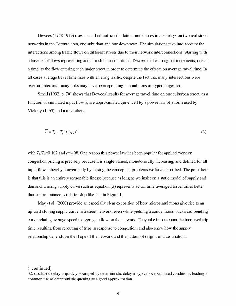
Dewees (1978 1979) uses a standard traffic-simulation model to estimate delays on two real street

networks in the Toronto area, one suburban and one downtown. The simulations take into account the

interactions among traffic flows on different streets due to their network interconnections. Starting with

a base set of flows representing actual rush hour conditions, Dewees makes marginal increments, one at

a time, to the flow entering each major street in order to determine the effects on average travel time. In

all cases average travel time rises with entering traffic, despite the fact that many intersections were

oversaturated and many links may have been operating in conditions of hypercongestion.

Small (1992, p. 70) shows that Dewees' results for average travel time on one suburban street, as a

function of simulated input flow λ, are approximated quite well by a power law of a form used by

Vickrey (1963) and many others:

with T1/T0=0.102 and ε=4.08. One reason this power law has been popular for applied work on

congestion pricing is precisely because it is single-valued, monotonically increasing, and defined for all

input flows, thereby conveniently bypassing the conceptual problems we have described. The point here

is that this is an entirely reasonable finesse because as long as we insist on a static model of supply and

demand, a rising supply curve such as equation (3) represents actual time-averaged travel times better

than an instantaneous relationship like that in Figure 1.

May et al. (2000) provide an especially clear exposition of how microsimulations give rise to an

upward-sloping supply curve in a street network, even while yielding a conventional backward-bending

curve relating average speed to aggregate flow on the network. They take into account the increased trip

time resulting from rerouting of trips in response to congestion, and also show how the supply

relationship depends on the shape of the network and the pattern of origins and destinations.

(..continued) 32, stochastic delay is quickly swamped by deterministic delay in typical oversaturated conditions, leading to common use of deterministic queuing as a good approximation.

ελ )/(10 bqTTT += (3)

10

Modeling Hypercongestion on a Straight Uniform Highway

We now turn to the search for dynamic models that deal with hypercongestion, yet are tractable

enough to be part of a toolkit for broader economic analysis. We begin with the straight uniform

highway, making two alternate assumptions about demand: first that the timing of the peak is

exogenous, and second that the timing is determined by scheduling costs. We are interested in travel-

time cost, which is travel time multiplied by the unit cost of travel delay, α.

Exogenous Demand Spike

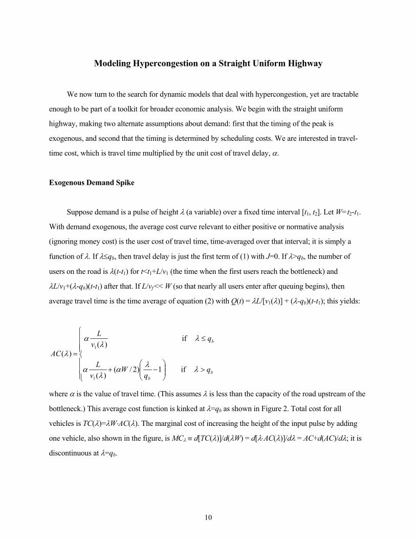
Suppose demand is a pulse of height λ (a variable) over a fixed time interval [t1, t2]. Let W=t2-t1.

With demand exogenous, the average cost curve relevant to either positive or normative analysis

(ignoring money cost) is the user cost of travel time, time-averaged over that interval; it is simply a

function of λ. If λ≤qb, then travel delay is just the first term of (1) with J=0. If λ>qb, the number of

users on the road is λ(t-t1) for t<t1+L/v1 (the time when the first users reach the bottleneck) and

λL/v1+(λ-qb)(t-t1) after that. If L/vf << W (so that nearly all users enter after queuing begins), then

average travel time is the time average of equation (2) with Q(t) = λL/[v1(λ)] + (λ-qb)(t-t1); this yields:

>

−+

≤

=

if 1)2/()(

if)(

)(

1

1

bb

b

qq

Wv

L

qv

L

AC

λλαλ

α

λλ

α

λ

where α is the value of travel time. (This assumes λ is less than the capacity of the road upstream of the

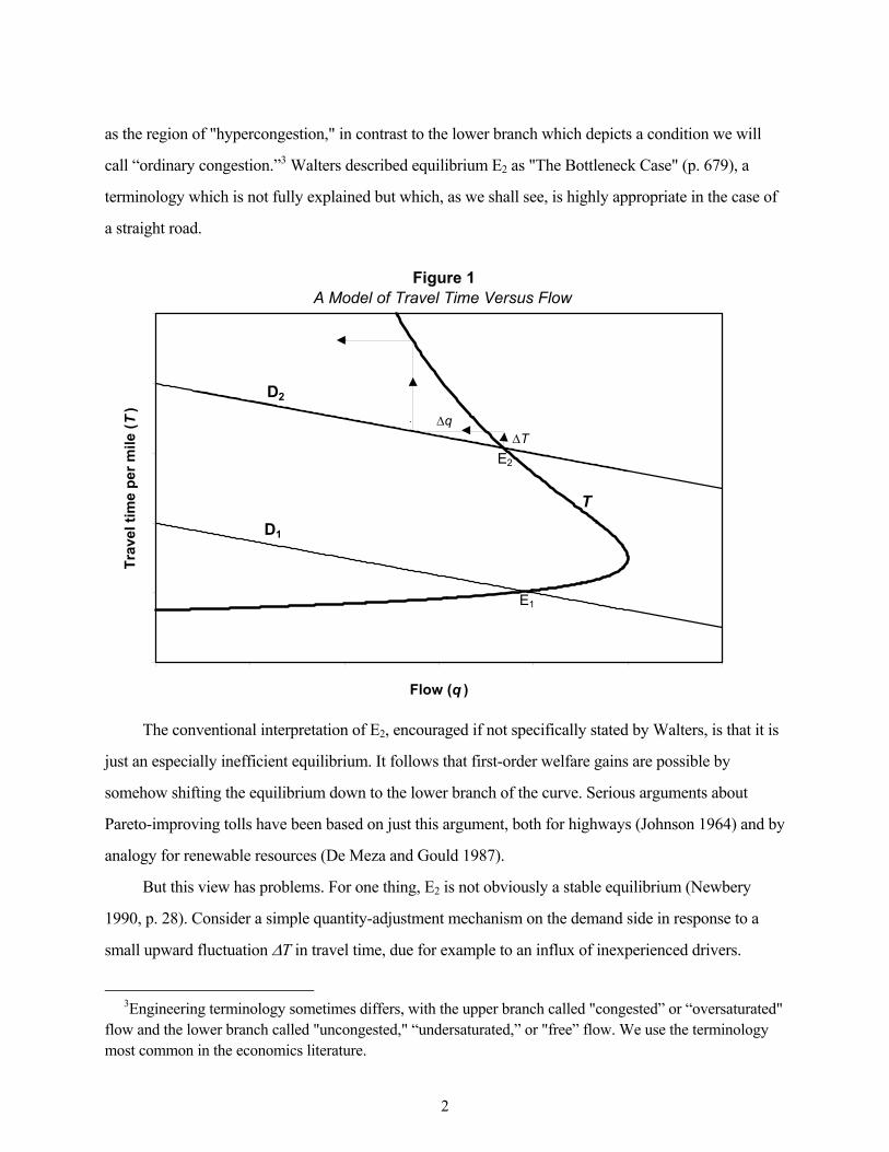
bottleneck.) This average cost function is kinked at λ=qb as shown in Figure 2. Total cost for all

vehicles is TC(λ)=λW⋅AC(λ). The marginal cost of increasing the height of the input pulse by adding

one vehicle, also shown in the figure, is MCλ ≡ d[TC(λ)]/d(λW) = d[λ⋅AC(λ)]/dλ = AC+d(AC)/dλ; it is

discontinuous at λ=qb.

11

In the region without hypercongestion (λ≤qb), average cost is rising modestly; marginal cost

exceeds it as in the conventional analysis. When λ>qb, marginal cost exceeds average cost by an

additional amount ½αWλ/qb, which is the optimal time-invariant toll associated with the queue and is

proportional to N≡λW, the total number of vehicles.15

It is clear from Figure 2 that, depending on the location of the demand curve, optimal inflow λ*

could be less than, equal to, or greater than bottleneck capacity. If it is greater, then hypercongestion

occurs, but only within the queue.16 If it is equal (a corner solution), then the external cost is interpreted

as the value of trips foregone due to the capacity constraint that is effectively imposed in this

optimum — that is, it is the vertical gap between the demand curve and the AC curve. These and other

pricing implications are considered by Mun (1999).

15This additional amount is calculated as λ times the derivative of the last term in the second line of the equation for AC(λ). It is in addition to the difference between MC and AC arising from the first term in that line. 16Queueing can be optimal in this case because the duration and shape of the demand pulse are assumed exogenous.

Figure 2Cost Versus Inflow: Long Uniform Road with Bottleneck

Exogenous Demand Pulse

Input flow (λ )

Cos

t per

veh

icle

AC

MC λ

q b

αλ W

α L v 1(0)

2q b

12

We can further simplify by making speed v1(λ) constant, justified by recent empirical findings

which indicate that the speed-flow relationship is quite flat in the region of ordinary congestion (TRB

1992). Then the curves in Figure 2 become piecewise linear, and are perfectly flat in the region of

ordinary congestion. Such a cost function is shown by Small (1992) to give a reasonably good fit to

Dewees' Toronto arterial data discussed earlier, as well as to some additional data from Boston

expressways. This model was used in an application to a San Francisco Bay Area freeway by Small

(1983). It turned out that in the San Francisco simulations, optimal flow was frequently equal to

capacity and never exceeded it, suggesting that the vertical section of the marginal cost curve was quite

high.

Endogenous Demand Pattern

Given that the road is well approximated by a point bottleneck, the endogenous trip scheduling

analysis begun by Vickrey (1969), provides an attractive alternative specification of how demand

becomes expressed as entering flow rates.17 We review it here because our model in the next section

builds on the same approach.

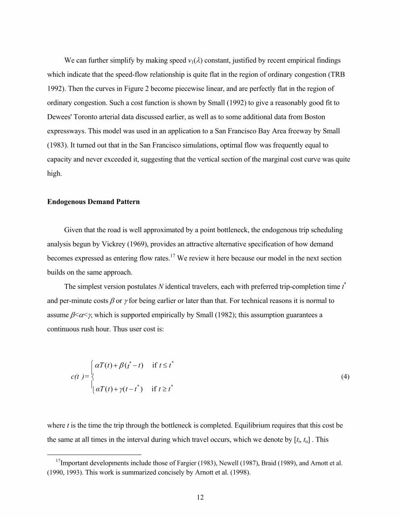
The simplest version postulates N identical travelers, each with preferred trip-completion time t*

and per-minute costs β or γ for being earlier or later than that. For technical reasons it is normal to

assume β<α<γ, which is supported empirically by Small (1982); this assumption guarantees a

continuous rush hour. Thus user cost is:

where t is the time the trip through the bottleneck is completed. Equilibrium requires that this cost be

the same at all times in the interval during which travel occurs, which we denote by [ti, tu] . This

17Important developments include those of Fargier (1983), Newell (1987), Braid (1989), and Arnott et al. (1990, 1993). This work is summarized concisely by Arnott et al. (1998).

≥−+

≤−+

**

*

if )()(

if)()(

ttttγtαT

tt tttT = ) c(t

*βα (4)

13

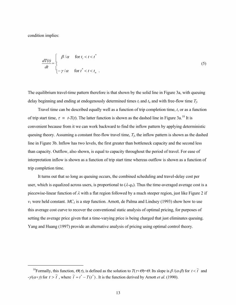
condition implies:

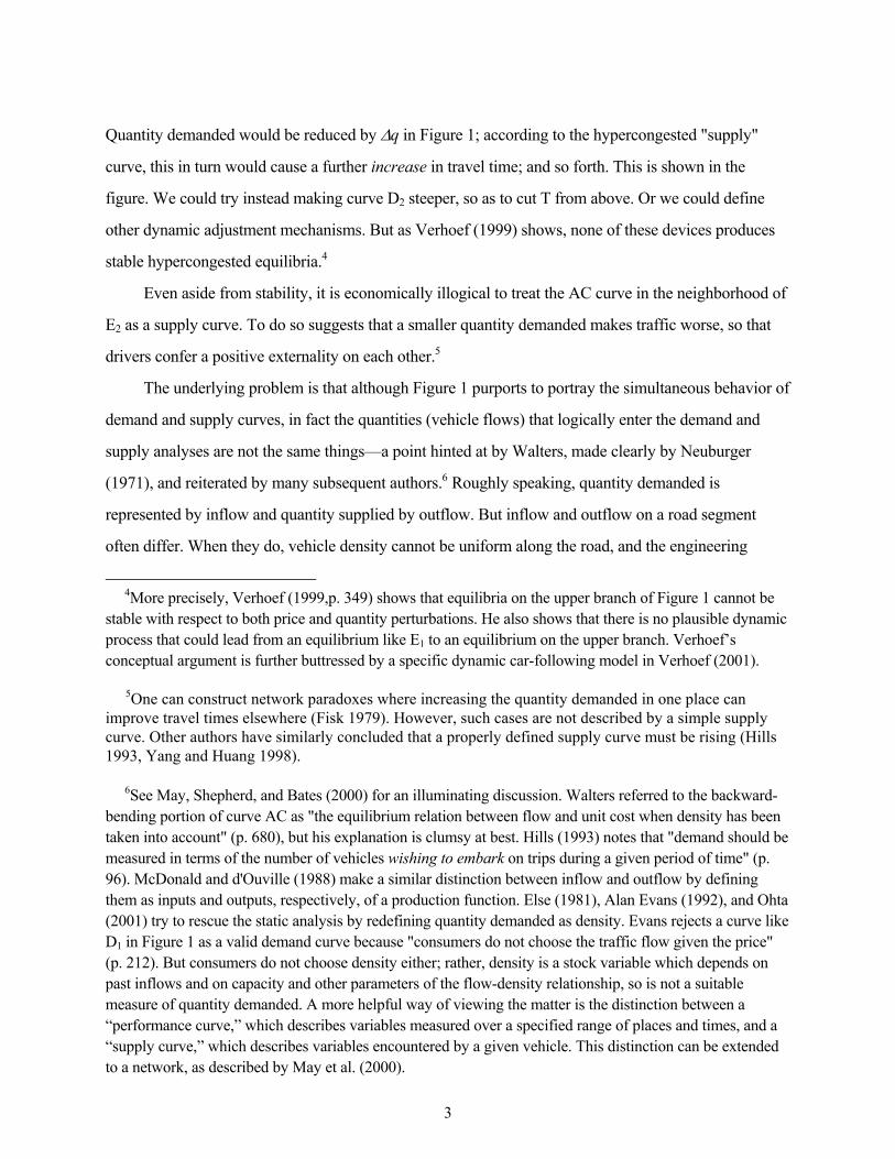
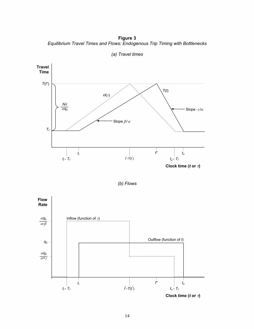
The equilibrium travel-time pattern therefore is that shown by the solid line in Figure 3a, with queuing

delay beginning and ending at endogenously determined times ti and tu and with free-flow time Tf.

Travel time can be described equally well as a function of trip completion time, t, or as a function

of trip start time, τ ≡ t-T(t). The latter function is shown as the dashed line in Figure 3a.18 It is

convenient because from it we can work backward to find the inflow pattern by applying deterministic

queuing theory. Assuming a constant free-flow travel time, Tf, the inflow pattern is shown as the dashed

line in Figure 3b. Inflow has two levels, the first greater than bottleneck capacity and the second less

than capacity. Outflow, also shown, is equal to capacity throughout the period of travel. For ease of

interpretation inflow is shown as a function of trip start time whereas outflow is shown as a function of

trip completion time.

It turns out that so long as queuing occurs, the combined scheduling and travel-delay cost per

user, which is equalized across users, is proportional to (λ-qb). Thus the time-averaged average cost is a

piecewise-linear function of λ with a flat region followed by a much steeper region, just like Figure 2 if

v1 were held constant. MCλ is a step function. Arnott, de Palma and Lindsey (1993) show how to use

this average cost curve to recover the conventional static analysis of optimal pricing, for purposes of

setting the average price given that a time-varying price is being charged that just eliminates queuing.

Yang and Huang (1997) provide an alternative analysis of pricing using optimal control theory.

18Formally, this function, Θ(τ), is defined as the solution to T(τ+Θ)=Θ. Its slope is β /(α-β) for tt ~< and -γ/(α+γ) for tt ~> , where )(~ ** tTtt −= . It is the function derived by Arnott et al. (1990).

<<−

<<

. for /

for /

*

*

u

i

ttt

ttt =

dtdT(t)

αγ

αβ (5)

14

Figure 3 Equilibrium Travel Times and Flows: Endogenous Trip Timing with Bottlenecks

(a) Travel times

(b) Flows

αqb α-β

ti - Tf t*-T(t*) tu - Tf ti t* tu

Clock time (t or τ)

ti - Tf t*-T(t*) tu - Tf ti t* tu

Clock time (t or τ)

Nδ αqb

αqb α+γ

Inflow (function of τ)

Outflow (function of t) qb

Travel Time

T(t*)

Tf

Slope β / α

Θ(τ)T(t)

Slope -γ /α

Flow Rate

15

Modeling Hypercongestion in a Dense Street Network

Networks of city streets, unlike freeways, are prone to slowdowns in which various flows

interfere with each other. As already noted, this phenomenon implies the existence of numerous local

queues. But they would not obey the laws of deterministic queuing at an isolated bottleneck; rather,

individual queue discharge rates are likely to depend on traffic density in neighboring parts of the

network due to cross traffic. We can therefore envision a system in which density builds up when total

input flow exceeds total exit flow, with the latter depending on the average density within the network.

Vickrey (1994) terms this appraoch a "bathtub model," although the analogy would seem to require

debris which clogs the drain when the water level gets too high. Perhaps a better analogy is to a messy

desk: the bigger the backlog of work, the harder it is to find papers and consequently processing slows

down.

To formalize this notion, we adapt a supply model used by Agnew (1977) and Mahmassani and

Herman (1984). We think of our model as approximating conditions in a central business district

(CBD). Trips inside the CBD begin and end either at its borders or at parking spaces within. The CBD

contains M lane-miles of streets, and average trip length is L. Vehicles enter the CBD streets at some

rate λ(t) vehicles per hour. At any time t traffic is characterized by two spatially aggregated variables:

per-lane density k(t) (vehicles per lane-mile), and average speed v(t) (miles per hour). We make the

following assumptions:

A1. Vehicle flow rate: Vehicles exit the streets at rate (M/L)q(t), where

Equation (6) defines q(t) (measured in vehicles per hour per lane) as an average per-lane flow rate. The

idea is that cars "leak out" by exiting the system at a rate proportional to q(t) such that in a steady state,

with entry and exit rates equal and constant at λ, density is constant at (L/M)(λ/v).

A2. Speed-density relationship: Average speed is related instantaneously to density by a functional

)()()( tvtktq = . (6)

16

relationship V(⋅):

That is, the fundamental diagram applies instantaneously in the aggregate. The function V is assumed to

satisfy V′<0 and kV′′+2V′<0 for all k. This guarantees that flow kv is a single-humped function of k,

rising from zero (at k=0) to a maximum qm at some value km, then falling to zero at a density kj known

as the "jam density;" the region where it is falling is known as hypercongestion. Assumption A2 makes

this an “instant-propagation” model in the terminology of Lindsey and Verhoef (2000), since an

increase in density anywhere lowers speeds immediately throughout the system.

A3. Conservation of vehicles: Vehicles appear or disappear in the system only through the entry and

exit flows already identified; that is, the number of vehicles changes according to:

For the speed-density relationship (7), we adopt the empirical relationship measured by Ardekani

and Herman (1987) from combined ground and air observations of the central business districts of Austin

and Dallas, Texas. The functional form comes from the "two-fluid" theory of Herman and Prigogine

(1979), in which moving vehicles and stopped vehicles follow distinct laws of motion. Letting K denote

the "normalized density" k/kj, the Ardekani-Herman (AH) formula is:

19This is a special case of their more general equation 7b when n=1, which is very close to the empirical value n=0.95 estimated for Dallas. We denote their expression vm(1-fs,min)1+ρ by vf. The Ardekani-Herman relationship is an example of a network-wide performance curve, from which we are deriving a dynamic supply relationship (see note 6).

)]([)( tkVtv = . (7)

)()/()()( tqLMt=dt

tdkM −λ . (8)

[ ] )(1)( 1tK v=tv +f − ρ (9)

where vf is the free-flow speed and ρ is an additional parameter.19 This formula implies a

maximum flow of:

17

occurring at density

We now proceed to apply this supply model to the same two demand models considered in the

previous section: first an exogenous demand spike, then an endogenous demand pattern generated by

linear scheduling costs.

Exogenous Demand Spike

Assume again that commuters enter the CBD network at a uniform rate λ over a fixed peak period

[t1,t2]. We use a linear speed-density relationship proposed by Greenshields (1935), which is a special

case of the AH formula for ρ=0:

)1( Kvv f −= . (12)

This simple relationship implies that flow is a quadratic function of speed; the congested and

hypercongested branches are the two roots of the quadratic. Maximum flow qm=¼vfkj occurs at density

km=½kj. The Greenshields relationship was the basis for Figure 1, and is used frequently in the

engineering and economics literatures on congestion, for example Newbery (1990, p. 28).

By substituting (6) and (12) into (8), we obtain a differential equation in normalized density that

applies for t1<t<t2:

ρ

ρ

ρρ

+

+

++

2

1

)2()1(

kv=q jfm (10)

ρ+k=k j

m 2. (11)

18

where µm ≡ (M/L)qm = ¼(M/L)vfkj is the maximum possible exit flow (completed trips per hour) and

Tf ≡ L/vf is the free-flow trip time for the average user. The boundary condition is K(t1)=0. After t2, the

same equation applies but with λ replaced by zero and with boundary condition that density be

continuous at t2.

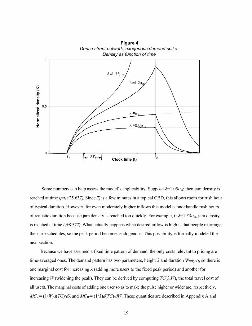
The solution for K(t) is provided in Appendix A and shown in Figure 4 for the case W=10Tf. Its

broad properties can be inferred just by inspecting equation (13). Recall that the term -K(1-K) is zero

when K=0 or K=1, and it reaches its most negative value when K=1/2. The curve portraying density

K(t) therefore starts upward at time t1 with initial slope λ/(4µmTf). As time progresses the curve becomes

flatter due to the term -K(1-K), then becomes steeper again when and if K increases beyond ½. At time

t2, the slope undergoes a discontinuity and becomes negative, the curve being steepest near K=½ but

then flattening and approaching zero asymptotically. Thus we have a period of density buildup during

time interval [t1, t2] followed by a gradual relaxation back toward free-flow conditions.

The solution has different regimes depending on the value of λ. If 맵m, normalized density

builds asymptotically to a value less than or equal to ½. Thus hypercongestion does not occur, and the

inflows can be maintained indefinitely. (The dashed curves in the figure show the paths that would be

taken if the inflow were not ended at t2.) But if λ>µm, the system reaches maximum outflow qm with

inflow still exceeding qm. At this point density builds up precipitously. This is the region of

hypercongestion, and outflow declines steadily. If t2 comes soon enough, a rather long discharge period

begins: it is especially long if K has reached a value near unity so that K(1-K) in (13) is small, indicating

a condition where outflow is nearly blocked. If t2 exceeds a "jam time" tj, whose value is given in the

Appendix, density reaches jam density (K=1) and the system breaks down: no more vehicles can enter.

This applies to the leftmost curve in Figure 4.

)1(4

KKµ

=dtdK

T m

f −−λ (13)

19

Some numbers can help assess the model’s applicability. Suppose λ=1.05µm; then jam density is

reached at time tj=t1+25.63Tf. Since Tf is a few minutes in a typical CBD, this allows room for rush hour

of typical duration. However, for even moderately higher inflows this model cannot handle rush hours

of realistic duration because jam density is reached too quickly. For example, if λ=1.33µm, jam density

is reached at time t1+8.57Tf. What actually happens when desired inflow is high is that people rearrange

their trip schedules, so the peak period becomes endogenous. This possibility is formally modeled the

next section.

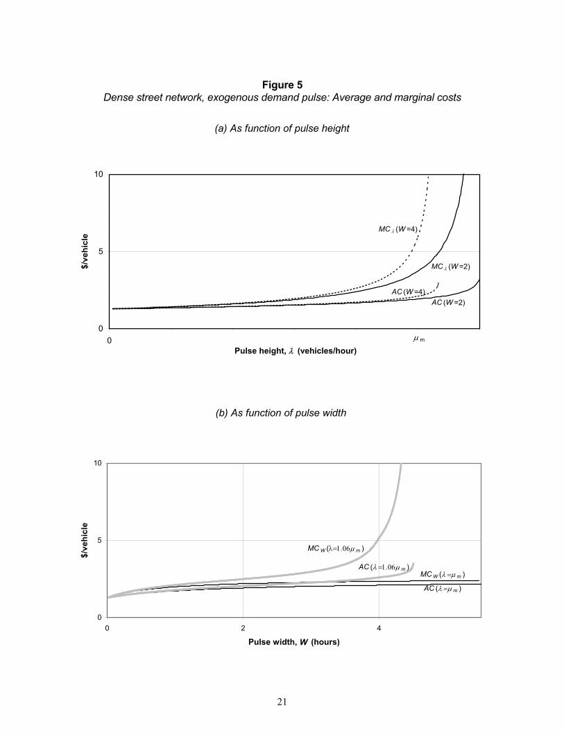
Because we have assumed a fixed time pattern of demand, the only costs relevant to pricing are

time-averaged ones. The demand pattern has two parameters, height λ and duration W≡t2-t1, so there is

one marginal cost for increasing λ (adding more users to the fixed peak period) and another for

increasing W (widening the peak). They can be derived by computing TC(λ,W), the total travel cost of

all users. The marginal costs of adding one user so as to make the pulse higher or wider are, respectively,

MCλ ≡ (1/W)d(TC)/dλ and MCW ≡ (1/λ)d(TC)/dW. These quantities are described in Appendix A and

Figure 4Dense street network, exogenous demand spike:

Density as function of time

0

0.5

1

Clock time (t)

Nor

mal

ized

den

sity

(K)

λ =0.8µ m

λ =µ m

λ =1.2µm

λ =1.33µm

t 1 t 22T f

20

are portrayed in Figures 5a and 5b, respectively, along with average cost AC≡TC/(λW). These curves

demonstrate how dynamics with hypercongestion still produce a rising supply curve. Indeed, Figure 5

looks very much like the conventional static analysis of congestion. For example, both MCλ and MCW

approach infinity at a critical value of λ or W, namely that for which K(t2)=1.

Endogenous Demand Pattern

Here we apply the “bottleneck model” of endogenous scheduling, described earlier, to a

hypercongested street network. Our starting point is Assumptions A1-A2 of the previous section, which

implicitly define a speed-flow relationship. To include Assumption A3, however, would be

incompatible with the bottleneck model. The latter requires identical individuals, all with the same trip

distance L. But A1-A3 together imply a distribution of trip distances: for example, as we saw in the last

section, after the input flow has fallen to zero the output flow falls to zero only asymptotically, implying

there are some very long trips.

We therefore replace A3 with two assumptions, the second of which is really an approximation.

A3′. Boundary conditions on density: Density k(t) is continuous everywhere, and non-zero only during

a finite time interval [ti, tu] when the flow of travelers reaching their destinations is non-zero.

Assumption A3′ cannot be reasonable unless the rush hour lasts considerably longer than free-

flow trip time L/vf. In our numerical simulation, the rush hour lasts 1.7 hours, whereas L/vf is 0.2 hours.

A4. Approximation for travel time: The travel time for a trip completed at time t can be approximated

by:

)()(

tvL=tT . (14)

21

Figure 5 Dense street network, exogenous demand pulse: Average and marginal costs

(a) As function of pulse height

0

5

10

0Pulse height, λ (vehicles/hour)

$/ve

hicl

e

MC λ (W =2)

AC (W =2)

MC λ (W =4)

AC (W =4)

µ m

(b) As function of pulse width

0

5

10

0 2 4

Pulse width, W (hours)

$/ve

hicl

e

MC W (λ =µ m )

AC (λ =µ m )

AC (λ =1.06µ m )

MC W (λ=1.06µ m )

22

Henderson (1981), Mahmassani and Herman (1984), and Yang and Huang (1997) all make an

approximation like A4, in which the travel time for an entire trip is determined by the speed

encountered at one point in the trip. The only difference is that for technical reasons, we take this point

to be the end rather than the beginning of the trip; since trip completion time t and trip start time τ are

fully determined functions of each other, the two alternate assumptions are equally strong.

Assumption A4 is drastic and its use by Mahmassani and Herman provoked vehement objection by

Newell (1988).20 But it dramatically simplifies the problem. Furthermore, its adequacy can be assessed

within the model itself. Once the system is solved for density k(t) using these assumptions, we can

compute from (7) the average speed at each point in time, v(⋅). We can then follow a car completing its

trip at time t backward through the system and compute its travel time T*(t) as the solution to:

(Mahmassani and Herman in fact seem to have computed trip times this way, apparently without

realizing that a different pattern of trip times was already implicit in their method for solving the

system.) We report this calculation in our simulations below.

The equilibrium travel-time pattern T(t) is completely determined by the requirement that total

trip cost be the same for everyone. This is just as in the bottleneck model described earlier, and the

result is exactly the triangular-shaped pattern of travel times already shown in Figure 3a. Given A4, T(t)

fully determines the pattern of average speeds, v(t). The pattern of flows, however, is quite different

than in the bottleneck model; hence so are the duration of the rush hour and the maximum travel delay.

This is because the exit rate of vehicles during the period of congestion is no longer constant at

bottleneck capacity, but instead is determined by (6) and (7).

We solve the system in Appendix B, using the Ardekani-Herman speed-density relationship of

equation (9). Figure 6 and Table 1 show some results for a particular set of parameters pertaining to the

20These authors focus on speed at the time the trip begins. However, Chu (1994, 1995) shows that in order to obtain an unpriced equilibrium, one needs instead to assume the speed when the trip ends determines trip time. Otherwise, travel time falls discontinuously at the end of the rush hour; the last traveler could not then be in equilibrium because he or she could be overtaken by a vehicle leaving slightly later. These technical problems do not affect Yang and Huang (1997) because they do not consider the unpriced equilibrium. The problems arise because scheduling costs are assumed to depend on trip completion time; presumably the situation would be reversed if scheduling costs were determined by deviation from a desired trip start time, as one might postulate for an afternoon rush hour.

L=tdtv t

(t)T-t

′′∫ )(*

. (15)

23

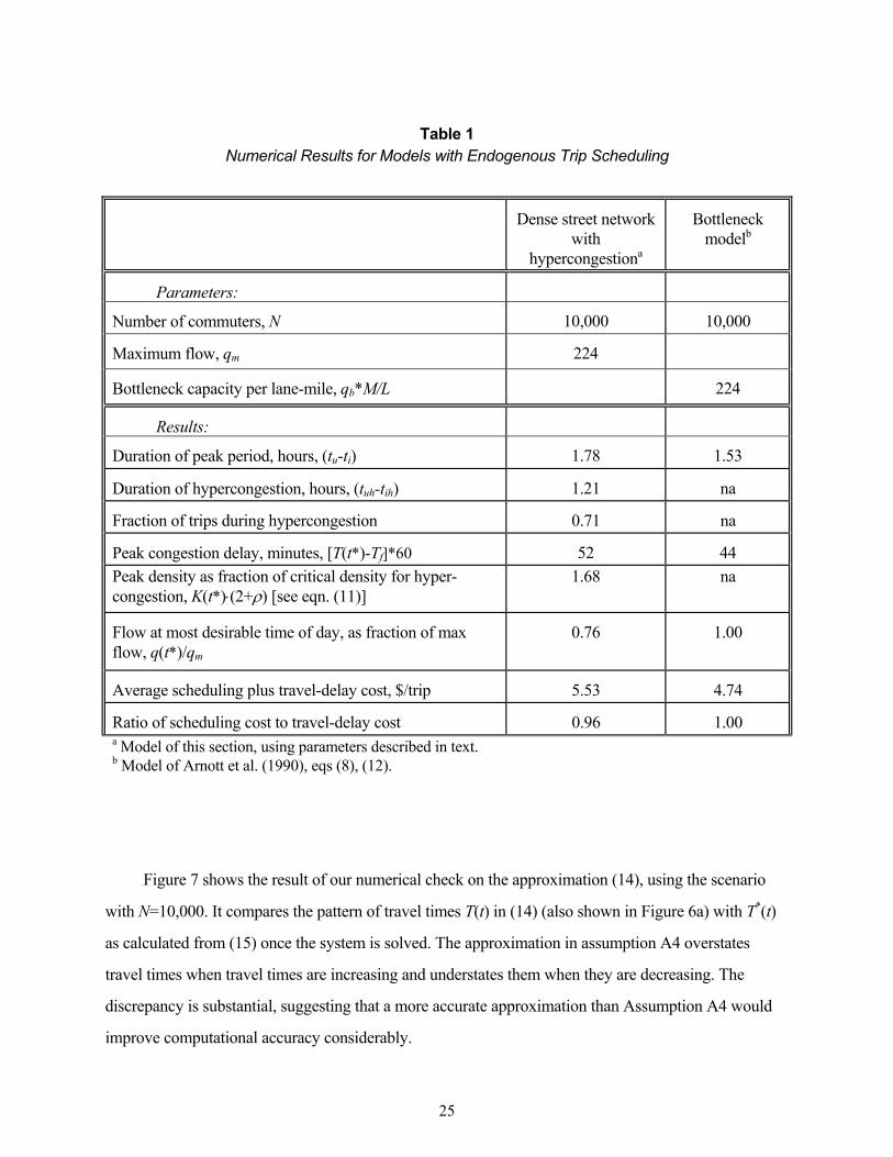
Dallas CBD,21 along with scheduling and travel-time cost parameters from Arnott et al. (1990)22 and

certain arbitrarily chosen values: t*=8.00 hours, L=4 miles, and N=10,000 vehicles. The bottleneck

model is calculated for a bottleneck capacity qb of (M/L)qm, so that the two models have identical values

of maximum flow.

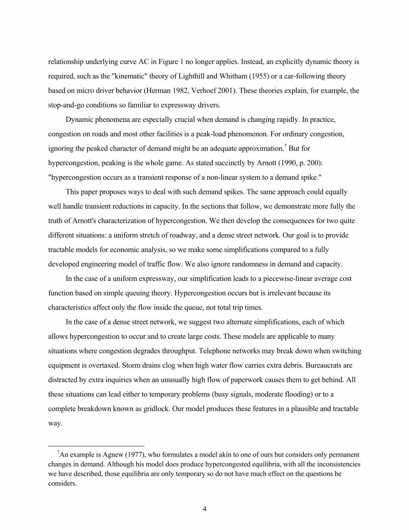
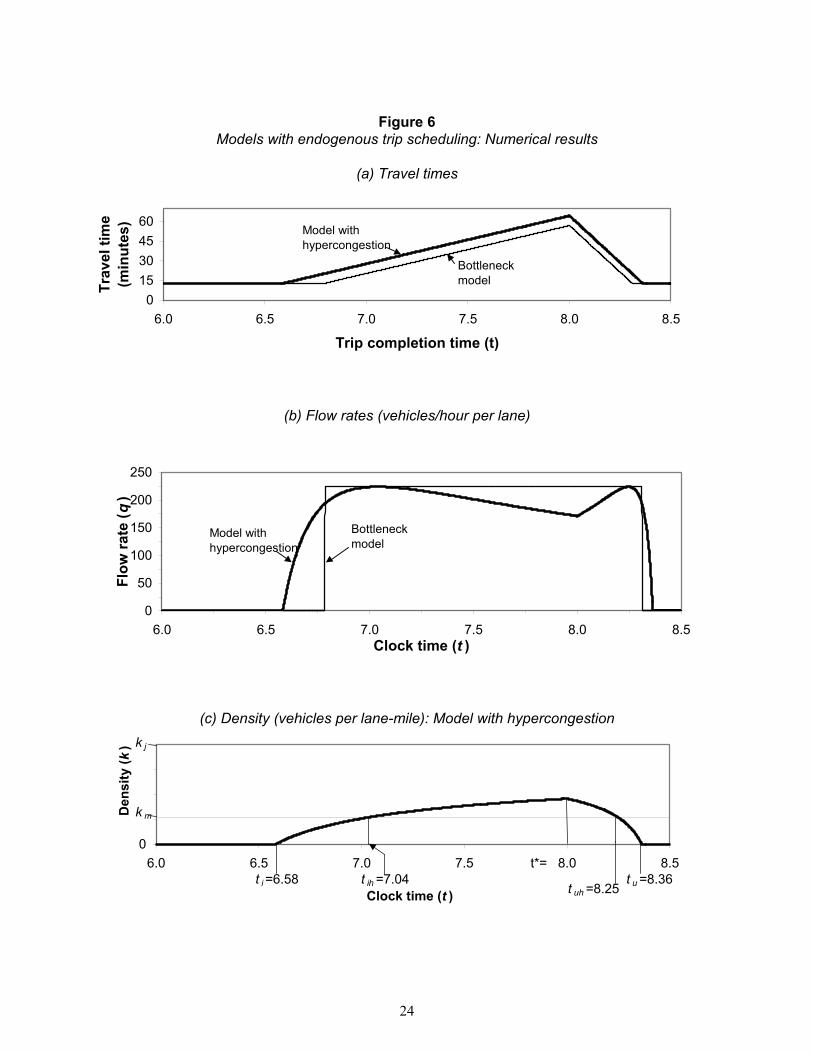
The model with hypercongestion generates more travel delays than the bottleneck model—52

versus 44 minutes at the height of the peak—and the rush hour lasts longer. The travel-time pattern

follows directly from the equilibrium condition for travelers with piecewise-linear costs of undesirable

schedules, so it has the same triangular shape in both models. However, the flow rate (which according

to A1 is proportional to the arrival rate of vehicles at their destinations) is different in the

hypercongestion model. It rises to the maximum possible amount, then is depressed by up to 24 percent

during the busiest time, then rises again to its maximum before finally dropping quickly to zero. The

times when flow is depressed is also the period, shown in the bottom panel, during which density

exceeds the value corresponding to maximum flow. The ability to predict a pattern of densities that can

be compared with actual measurements is a useful feature of our model, one that is lacking in the

bottleneck model.

We see from Table 1 that total congestion cost (travel delay plus scheduling) is about 17 percent

higher due to hypercongestion. Interestingly, however, it remains about equally comprised of

scheduling cost and travel-delay cost, their ratio being 0.96 compared to exactly 1.0 in the bottleneck

model.

21These are: M=117 lane-miles; qm =224 vehicles/lane-hour; kj=100 vehicles/lane-mile; and ρ =1.67, all taken from Ardekani and Herman (1987), p. 9 and legend to Fig. 4. The implied free-flow speed from (12) is vf=19.22 mi./hr.; maximum flow occurs at density km=27 vehicles per lane-mile and at speed 8.2 miles/hour.

22Namely α=$6.40/hour, β=0.609α, and γ=2.377α. The latter two ratios are derived from Small (1982).

24

Figure 6 Models with endogenous trip scheduling: Numerical results

(a) Travel times

(b) Flow rates (vehicles/hour per lane)

(c) Density (vehicles per lane-mile): Model with hypercongestion

0

50

100

150

200

250

6.0 6.5 7.0 7.5 8.0 8.5Clock time (t )

Flow

rate

( q)

Model with hypercongestion

Bottleneck model

015304560

6.0 6.5 7.0 7.5 8.0 8.5

Trip completion time (t)

Trav

el ti

me

(min

utes

) Model with hypercongestion

Bottleneck model

06.0 6.5 7.0 7.5 8.0 8.5

Clock time (t )

Den

sity

( k) k j

k m

t ih =7.04t*=

t uh =8.25t i =6.58 t u =8.36

25

Table 1 Numerical Results for Models with Endogenous Trip Scheduling

Dense street network with

hypercongestiona

Bottleneck modelb

Parameters:

Number of commuters, N 10,000 10,000

Maximum flow, qm 224

Bottleneck capacity per lane-mile, qb*M/L 224

Results:

Duration of peak period, hours, (tu-ti) 1.78 1.53

Duration of hypercongestion, hours, (tuh-tih) 1.21 na

Fraction of trips during hypercongestion 0.71 na

Peak congestion delay, minutes, [T(t*)-Tf]*60 52 44 Peak density as fraction of critical density for hyper-congestion, K(t*)⋅(2+ρ) [see eqn. (11)]

1.68 na

Flow at most desirable time of day, as fraction of max flow, q(t*)/qm

0.76 1.00

Average scheduling plus travel-delay cost, $/trip 5.53 4.74

Ratio of scheduling cost to travel-delay cost 0.96 1.00 a Model of this section, using parameters described in text. b Model of Arnott et al. (1990), eqs (8), (12).

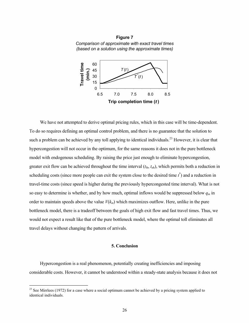
Figure 7 shows the result of our numerical check on the approximation (14), using the scenario

with N=10,000. It compares the pattern of travel times T(t) in (14) (also shown in Figure 6a) with T*(t)

as calculated from (15) once the system is solved. The approximation in assumption A4 overstates

travel times when travel times are increasing and understates them when they are decreasing. The

discrepancy is substantial, suggesting that a more accurate approximation than Assumption A4 would

improve computational accuracy considerably.

26

Figure 7 Comparison of approximate with exact travel times (based on a solution using the approximate times)

We have not attempted to derive optimal pricing rules, which in this case will be time-dependent.

To do so requires defining an optimal control problem, and there is no guarantee that the solution to

such a problem can be achieved by any toll applying to identical individuals.23 However, it is clear that

hypercongestion will not occur in the optimum, for the same reasons it does not in the pure bottleneck

model with endogenous scheduling. By raising the price just enough to eliminate hypercongestion,

greater exit flow can be achieved throughout the time interval (tih, tuh), which permits both a reduction in

scheduling costs (since more people can exit the system close to the desired time t*) and a reduction in

travel-time costs (since speed is higher during the previously hypercongested time interval). What is not

so easy to determine is whether, and by how much, optimal inflows would be suppressed below qm in

order to maintain speeds above the value V(km) which maximizes outflow. Here, unlike in the pure

bottleneck model, there is a tradeoff between the goals of high exit flow and fast travel times. Thus, we

would not expect a result like that of the pure bottleneck model, where the optimal toll eliminates all

travel delays without changing the pattern of arrivals.

5. Conclusion

Hypercongestion is a real phenomenon, potentially creating inefficiencies and imposing

considerable costs. However, it cannot be understood within a steady-state analysis because it does not

23 See Mirrlees (1972) for a case where a social optimum cannot be achieved by a pricing system applied to identical individuals.

015304560

6.5 7.0 7.5 8.0 8.5

Trip completion time (t )

Trav

el ti

me

(min

.) T (t )

T *(t )

27

in practice persist as a steady state. Rather, hypercongestion occurs as a result of transient demand

surges and can be fully analyzed only within a dynamic model. Even if the dynamic model is converted

to a static one through the use of time averaging, the appropriate specification of average cost depends

on the underlying dynamics. In virtually all circumstances that specification will portray average cost as

a rising function of quantity demanded, even when hypercongestion occurs.

In one case, that of a uniform length of highway ending in a bottleneck, hypercongestion exists

but it just describes the density of vehicles within a queue and does not materially affect total travel

time.

In another case, that of a dense street network, it is plausible to model flow within a well-defined

area as subject to hypercongestion. We have shown that a dynamic model incorporating this feature can

be constructed and solved for two interesting special cases of the demand pattern. Doing so explains

features that we observe in real cities: the gradual buildup of vehicle density during a rush hour, with

dramatic and quite sudden slowdowns possible if density reaches the hypercongested region. A state of

total breakdown, where speed falls to zero, is theoretically possible: this is gridlock in its literal

meaning, with the various local queues on the network totally blocking each other. There is no way out

of gridlock within the model. However, severe congestion short of gridlock ultimately dissipates once

the demand surge abates.

One promising way to model these demand surges is by means of the endogenous scheduling

models that have worked their way prominently into both the economics and engineering literatures.

We show how ideas from these models can be applied to a dense street network subject to

hypercongestion.

28

References

Agnew, Carson E. (1977): "The Theory of Congestion Tolls," Journal of Regional Science, 17, 381-

393. Ardekani, Siamak, and Robert Herman (1987): "Urban Network-Wide Traffic Variables and Their

Relations," Transportation Science, 21, 1-16. Arnott, Richard (1979): "Optimal City Size in a Spatial Economy," Journal of Urban Economics, 6, 65-

89. Arnott, Richard (1990): "Signalized Intersection Queuing Theory and Central Business District Auto

Congestion," Economics Letter, 33, 197-201. Arnott, Richard, Andre de Palma, and C. Robin Lindsey (1990): "Economics of A Bottleneck," Journal

of Urban Economics, 27, 111-130. Arnott, Richard, Andre de Palma, and C. Robin Lindsey (1993): "A Structural Model of Peak-Period

Congestion: A Traffic Bottleneck with Elastic Demand," American Economic Review, 83, 161-179. Arnott, Richard, Andre de Palma, and C. Robin Lindsey (1998): "Recent Developments in the

Bottleneck Model," in Kenneth J. Button and Erik T. Verhoef, eds., Road Congestion, Traffic Congestion and the Environment: Issues of Efficiency and Social Feasibility. Cheltenham, UK: Edward Elgar, pp. 79-110.

Banks, James H. (1989): "Freeway Speed-Flow-Concentration Relationships: More Evidence and

Interpretations," Transportation Research Record, 1225, 53-60. Beckmann, Martin, C.B. McGuire, and Christopher B. Winsten (1955): Studies in the Economics of

Transportation. New Haven: Yale University Press. Berglas, Eitan, and David Pines (1981): "Clubs, Local Public Goods and Transportation Models—A

Synthesis," Journal of Public Economics, 15, 141-162. Boiteux, M. (1949): "La Tarification des Demandes en Pointe: Application de la Théorie de la Vente au

Coût Marginal," Revue Générale de l'Électricité, August. Reprinted in English translation as "Peak-Load Pricing," Journal of Business, 33 [1960], 157-179.

Braid, Ralph (1989): "Uniform versus Peak-Load Pricing of a Bottleneck with Elastic Demand,"

Journal of Urban Economics, 26, 320-327. Branston, David (1976): "Link Capacity Functions: A Review," Transportation Research, 10, 223-236. Cassidy, Michael J. (1998): "Bivariate Relations in Nearly Stationary Highway Traffic," Transportation

Research, 32B, 49-59. Cassidy, Michael J., and Robert L. Bertini (1999): "Some Traffic Features at Freeway Bottlenecks,"

29

Transportation Research, 33B, 25-42. Chu, Xuehao (1995): "Endogenous Trip Scheduling: The Henderson Approach Reformulated and

Compared with the Vickrey Approach," Journal of Urban Economics, 37, 324-343. Chu, Xuehao (1994): "A Structural Model of Hypercongestion for Street-Network Traffic," Center for

Urban Transportation Research. Daganzo, C.F., M.J. Cassidy, and R.L. Bertini (1999): "Possible Explanations of Phase Transitions in

Highway Traffic," Transportation Research, 33A, 365-379. De Meza, David, and J.R. Gould (1987): "Free Access versus Private Property in a Resource: Income

Distributions Compared," Journal of Political Economy, 95, 1317-1325. DeVany, Arthur S., and Thomas R. Saving (1980): "Competition and Highway Pricing for Stochastic

Traffic," Journal of Business, 53, 45-60. Dewees, Donald N. (1978): "Simulations of Traffic Congestion in Toronto," Transportation Research,

12, 153-165. Dewees, Donald N. (1979): "Estimating the Time Costs of Highway Congestion," Econometrica, 47,

1499-1512. Edelson, Noel M. (1971): "Congestion Tolls Under Monopoly," American Economic Review, 61, 873-

882. Else, P.K. (1981): "A Reformulation of the Theory of Optimal Congestion Taxes," Journal of Transport

Economics and Policy, 15, 217-232. Evans, Alan W. (1992): "Road Congestion: The Diagrammatic Analysis," Journal of Political

Economy, 100, 211-217. Fargier, Paul-Henri (1983): "Effects of the Choice of Departure Time on Road Traffic Congestion," in

Proceedings of the Eighth International Symposium on Transportation and Traffic Theory, ed. by V.F. Hurdle, E. Hauer, and G.N. Steuart. Toronto: University of Toronto Press, 223-263.

Fisk, Caroline (1979): "More Paradoxes in the Equilibrium Assignment Problem," Transportation

Research, 13B, 305-309. Greenshields, B.D. (1935): "A Study of Traffic Capacity," Highway Research Board Proceedings, 14,

Part I, 448-477. Haight, Frank (1963): Mathematical Theories of Traffic Flow. New York: Academic Press. Hall, Fred L., and Lisa M. Hall (1990): "Capacity and Speed Flow Analysis of the QEW in Ontario,"

Transportation Research Record, 1287, 108-118. Hall, Fred L., V.F. Hurdle, and James H. Banks (1992): "Synthesis of Recent Work on the Nature of

30

Speed-Flow and Flow-Occupancy (or Density) Relationships on Freeways," Transportation Research Record, 1365, 12-18.

Hau, Timothy D. (1998): "Congestion Pricing and Road Investment," in Road Pricing, Traffic

Congestion and the Environment: Issues of Efficiency and Social Feasibility, ed. by Kenneth J. Button and Erik T. Verhoef. Cheltenham, UK: Edward Elgar, 39-78.

Helbing, Dirk, and Martin Treiber (1998): "Jams, Waves, and Clusters," Science, 282, 2001-2002. Henderson, J. Vernon (1981): "The Economics of Staggered Work Hours," Journal of Urban

Economics, 9, 349-364. Herman, Robert (1982): “Remarks on Traffic Flow Theories and rthe Characterization of Traffic in

Cities,” in William C. Schieve and Peter M. Allen, eds., Self-Organization and Dissipative Structures: Applications in the Physical and Social Sciences. University of Texas Press, Austin.

Herman, Robert, and Ilya Prigogine (1979): "A Two-Fluid Approach to Town Traffic," Science, 204,

148-151. Hills, Peter (1993): "Road Congestion Pricing: When Is It a Good Policy? A Comment," Journal of

Transport Economics and Policy, 27, 91-99. Hurdle, V.F., and Bongsoo Son (2001): “Shock Wave and Cumulative Arrival and Departure Models:

Partners without Conflict,” Transportation Research Record, 1776, 159-166. Johnson, M. Bruce (1964): "On the Economics of Road Congestion," Econometrica, 32, 137-150. Kerner, B.S., and H. Rehborn (1997): "Experimental Properties of Phase Transitions in Traffic Flow,"

Physical Review Letters, 79, 4030-4033. Knight, Frank (1924): "Some Fallacies in the Interpretation of Social Costs," Quarterly Journal of

Economics, 38, 582-606. Lévy-Lambert, H. (1968): "Tarification des Services à Qualité Variable—Application aux Péages de

Circulation," Econometrica, 36, 564-574. Lighthill, M.H., and G.B. Whitham (1955): "On Kinematic Waves, II: A Theory of Traffic Flow on

Long Crowded Roads," Proceedings of the Royal Society (London), A229, 317-345. Lindsey, Robin, and Erik Verhoef (2000): “Congestion Modeling,” in Handbooks in Transport, volume

1: Handbook of Transport Modelling, ed. by David A. Hensher and Kenneth J. Button, Elsevier, Amsterdam, ch. 21, 353-373.

Mahmassani, Hani, and Robert Herman (1984): "Dynamic User Equilibrium Departure Time and Route

Choice on Idealized Traffic Arterials," Transportation Science, 18, 362-384. Marchand, Maurice (1968): "A Note on Optimal Tolls in an Imperfect Environment," Econometrica,

36: 575-581.

31

May, Anthony D., S.P. Shepherd, and J.J. Bates (2000): "Supply Curves for Urban Road Networks,"

Journal of Transport Economics and Policy, 34, 261-290. McDonald, John F., and Edmond L. d'Ouville (1988): "Highway Traffic Flow and the 'Uneconomic'

Region of Production," Regional Science and Urban Economics, 18, 503-509. McDonald, John F., Edmond L. d'Ouville, and Louie Nan Liu (1999): Economics of Urban Highway

Congestion and Pricing. Kluwer Academic Publishers, Dordrecht. Mills, David E. (1981): "Ownership Arrangements and Congestion-Prone Facilities," American

Economic Review, 71, 493-502. Mirrlees, James A. (1972): “The Optimum Town,” Swedish Journal of Economics, 74, 114-135. Mohring, Herbert (1970): "The Peak Load Problem with Increasing Returns and Pricing Constraints,"

American Economic Review, 60, 693-705. Mun, Se-il (1994): "Traffic Jams and the Congestion Toll," Transportation Research B, 28, 365-375. Mun, Se-il (1999): "Peak-Load Pricing of a Bottleneck with Traffic Jam," Journal of Urban Economics,

46, 323-349. Mun, Si-il (2002): “Bottleneck Congestion with Traffic Jam,” working paper, Graduate School of

Economics, Kyoto University (November). Muñoz, Juan Carlos, and Carlos F. Daganzo (2002): "The Bottleneck Mechanism of a Freeway

Diverge," Transportation Research A, 36, 483-505. Neuburger, Henry (1971): "The Economics of Heavily Congested Roads," Transportation Research, 5,

283-293. Newbery, David M. (1990): "Pricing and Congestion: Economic Principles Relevant to Pricing Roads,"

Oxford Review of Economic Policy, 6, 22-38. Newell, Gordon F. (1987): "The Morning Commute for Nonidentical Travelers," Transportation

Science, 21, 74-88. Newell, Gordon F. (1988): "Traffic Flow for the Morning Commute," Transportation Science, 22, 47-

58. Oakland, William H. (1972): "Congestion, Public Goods and Welfare," Journal of Public Economics, 1,

339-357. Ohta, Hiroshi (2001): “Proving a Traffic Congestion Controversy: Density and Flow Scrutinized,”

Journal of Regional Science, 41, 659-680. Pigou, Arthur C. (1920): The Economics of Welfare. London: Macmillan.

32

Rouphail, Nagui M., and Rahmi Akçelik (1992): "Oversaturation Delay Estimates with Consideration

of Peaking," Transportation Research Record, 1365, 71-81. Small, Kenneth A. (1982): "The Scheduling of Consumer Activities: Work Trips," American Economic

Review, 72, 467-79. Small, Kenneth A. (1983): "Bus Priority and Congestion Pricing On Urban Expressways," in Research

in Transportation Economics, Vol. 1, ed. by Theodore E. Keeler. Greenwich, Connecticut: JAI Press, 27-74.

Small, Kenneth A. (1992): Urban Transportation Economics, Vol. 51 of Fundamentals of Pure and

Applied Economics series. Chur, Switzerland: Harwood Academic Press. TRB (1992): Highway Capacity Manual, 3rd edition. Transportation Research Board Special Report

209. Washington: National Academy Press. Verhoef, Erik T. (1999): "Time, Speeds, Flows and Densities in Static Models of Road Traffic

Congestion and Congestion Pricing," Regional Science and Urban Economics, 29, 341-369. Verhoef, Erik T. (2001): "An Integrated Dynamic Model of Road Traffic Congestion Based on Simple

Car-Following Theory: Exploring Hypercongestion," Journal of Urban Economics, 49, 505-542. Vickrey, William S. (1955): "Some Implications of Marginal Cost Pricing for Public Utilities,"

American Economic Review, Papers and Proceedings, 45, 605-620. Vickrey, William S. (1963): "Pricing in Urban and Suburban Transport," American Economic Review,

Papers and Proceedings, 53, 452-465. Vickrey, William (1969): "Congestion Theory and Transport Investment," American Economic Review,

59, 251-261. Vickrey, William (1994): "Types of Congestion Pricing Models," mimeo, Columbia University,

November. Walters, A.A. (1961): "The Theory and Measurement of Private and Social Cost of Highway

Congestion," Econometrica, 29, 676-699. Walters, A.A. (1987): "Congestion," in The New Palgrave: A Dictionary of Economics, Macmillan,

New York. Williams, James C., Hani S. Mahmassani, and Robert Herman (1987): "Urban Traffic Network Flow

Models," Transportation Research Record, 1112, 78-88. Williamson, Oliver E. (1966): "Peak-Load Pricing and Optimal Capacity under Indivisibility

Constraints," American Economic Review, 56, 810-827. Yang, Hai, and Hai-Jun Huang (1997): "Analysis of the Time-Varying Pricing of a Bottleneck with

33

Elastic Demand Using Optimal Control Theory," Transportation Research, 31B, 425-440. Yang, Hai, and Hai-Jun Huang (1998): "Principle of Marginal-Cost Pricing: How Does It Work in a

General Road Network?" Transportation Research, 32A, 45-54.

A-1

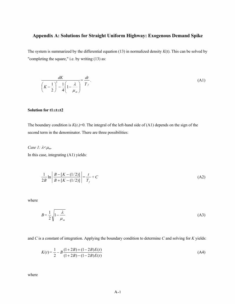
Appendix A: Solutions for Straight Uniform Highway: Exogenous Demand Spike

The system is summarized by the differential equation (13) in normalized density K(t). This can be solved by

"completing the square," i.e. by writing (13) as:

Solution for t1§t§t2

The boundary condition is K(t1)=0. The integral of the left-hand side of (A1) depends on the sign of the

second term in the denominator. There are three possibilities:

Case 1: λ<µm.

In this case, integrating (A1) yields:

where

and C is a constant of integration. Applying the boundary condition to determine C and solving for K yields:

where

. Tdt =

K

dK f

m

−−

−

µλ1

41

21 2 (A1)

CTt

KBKB

B

f

+ = )]2/1([)]2/1([ ln

21

−+−− (A2)

µλ

m

= B −121 (A3)

)()21()21()()21()21(

21)(

tEBBtEBBB=tK

−−+−++

− (A4)

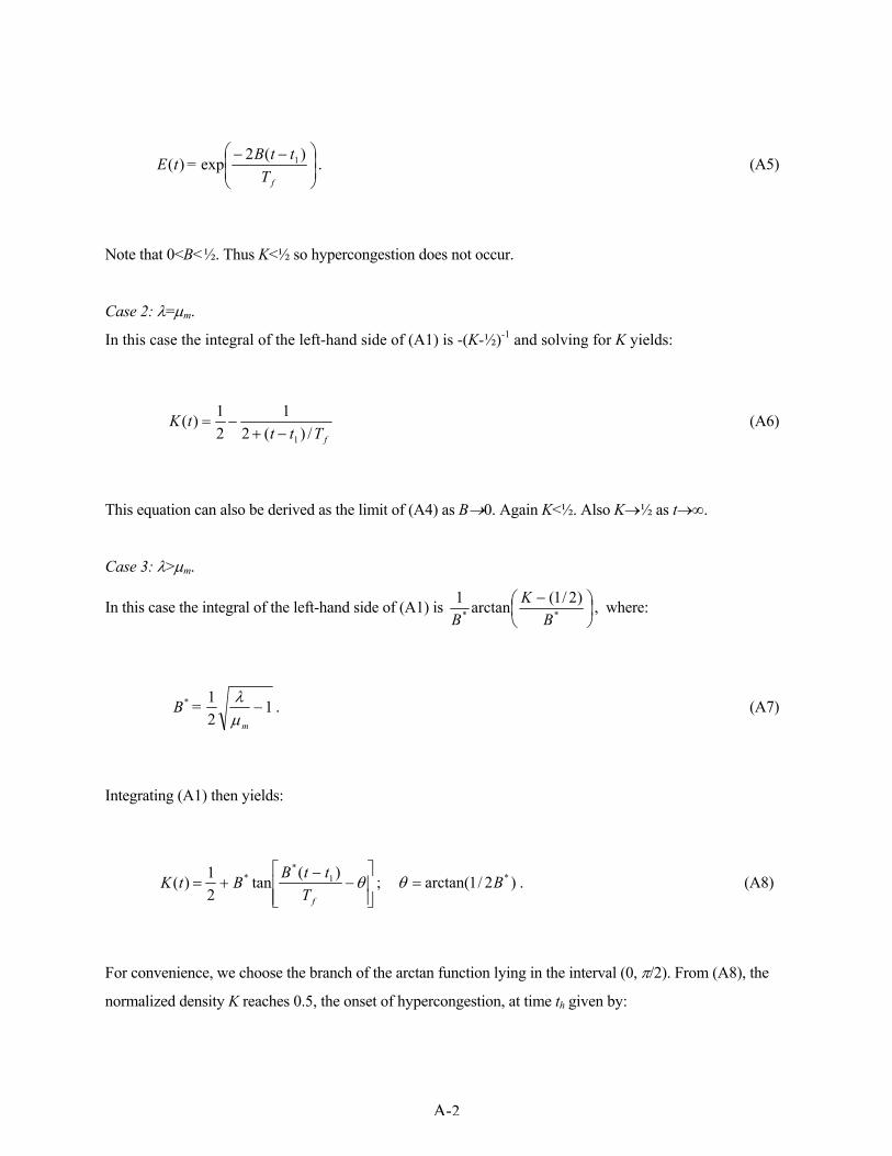
A-2

Note that 0<B<½. Thus K<½ so hypercongestion does not occur.

Case 2: λ=µm.

In this case the integral of the left-hand side of (A1) is -(K-½)-1 and solving for K yields:

This equation can also be derived as the limit of (A4) as B→0. Again K<½. Also K→½ as t→∞.

Case 3: λ>µm.

In this case the integral of the left-hand side of (A1) is

−

**

)2/1(arctan1B

KB

, where:

Integrating (A1) then yields:

For convenience, we choose the branch of the arctan function lying in the interval (0, π/2). From (A8), the

normalized density K reaches 0.5, the onset of hypercongestion, at time th given by:

−−

fTttB=tE )(2exp)( 1 . (A5)

fTtt

tK/)(2

121)(

1−+−= (A6)

121* −

µλ

m

= B . (A7)

−

−+= θ

fTttBBtK )(tan

21)( 1

** ; )2/1arctan( *B=θ . (A8)

A-3

and jam density is reached at time

. 2 arctan **

B

BT

+ t = t fhj (A9)

For t > tj the model breaks down and (A8) is no longer valid—in fact no solution can be given; in reality,

outside intervention is needed to halt inflow until the built-up density can be discharged.

Solution for t>t2

After the traffic pulse ends, the cars in the center will gradually dissipate. Assume t2<tj and define

K2≡K(t2), as determined from (A4), (A6), or (A8) as appropriate. Then density is determined by solving (A1)

again, this time with λ=0 and with the boundary condition that K(t2)=K2 . The solution is obtained from (A2)

by setting B=½ and choosing the constant of integration to meet the new boundary condition. The result is

This function is decreasing in t, approaches zero asymptotically, and has an inflection point when and if

K=½.

Total Cost

The total cost to all users is just the value of time, α, times the total number of user-hours spent in the

system:

θ*1 BT

tt fh +=

1

2

2

2 exp11)(−

−⋅

−+=

fTtt

KKtK . (A10)

A-4

Writing I1 for the part of the integral from t1 to t2, and integrating (A10) from t2 to ∞, this equation yields:

)]1log([ 21 KTIMkTC fj −−=α . (A11)

The integral I1 can be calculated as follows, where W≡t2-t1 is the pulse duration:

2/1 WI = if λ=µm ; (A12)

−+=

])/cos[()cos(log)2/(1 θ

θ

ff TBW

TWI if λ>µm .

For Figure 5, we have calculated the total cost from (A11) and (A12) and marginal costs using numerical

derivatives.

Appendix B. Solutions for Dense Street Network: Endogenous Demand Pattern

First, we formulate the differential equation that will determine normalized traffic density K(t).

Substituting (9) into (14), we differentiate the result to obtain the time derivative, dT/dt, that is consistent

with the flow dynamics:

But (5) gives the time derivative that is consistent with equilibrium in scheduling. Equating the two yields

∫∞

=1

)(t

j dttKMkTC α .

[ ])/2exp()21()21(log)4log(21

1 fff TBWBBTBTWB = I −−−+−+⋅

− if λ<µm ;

. dtdKK-1+1T =

dtdT f

)2())(( ρρ +− (B1)

A-5

the following differential equation in K(t):

where

>−

<=

.for )/(

for )/()(

*

*

ttT

ttTt

f

f

αγ

αβσ (B3)

Equation (B2) is solved (for fixed σ) by grouping terms in K and terms in t in the left- and right-hand sides,

respectively, and integrating to obtain:

which is valid separately for the two regions of t over which σ is constant. Solving (B4),

where σ is given by (B3) and C is another constant of integration.

The boundary conditions for the two regions t<t* and t>t* are, respectively, K(ti)=0 and K(tu)=0. Here

ti and tu are the times the first and last trips are completed and their values are still to be determined. These

conditions, along with the definition of σ, yield:

ρ

ρσ +−+

2)1(1

)( Kt = dtdK (B2)

)(1

1)1(

11

11 C+t

+=

K ⋅

−⋅

+ + σρρ ρ , (B4)

)1/(1)(1)( ρσ +−⋅− C+t= tK

A-6

The function K(t), and hence T(t), must be continuous at t*; thus

(We could have deduced this equality directly from the fact that the first and last travelers suffer no travel

delay and so must have equal scheduling costs.) Equation (B6) fixes t* within the interval [ti, tu]; it remains to

determine the width of this interval. This is done by integrating the exit flow (M/L)q(t) ≡

(Mkj/L)K(t)vf⋅[1-K(t)]1+ρ over the duration of the rush hour and setting the result equal to N, the exogenous

number of travelers. After much tedious calculation, this yields:

where

s ≡ β(t*-ti)/(αTf) ≡ γ(tu-t*)/(αTf) (B8)

is the ratio of schedule delay cost to travel-time cost for the first and last travelers (equalized according to

B6). Note that s is an indicator of how severe congestion is for the first and last travelers, hence for all

travelers. Equation (B7) implies:

<<

−+−

−+−

+

. for T

)(1 1

<<for )(11

*

f

)+/(11-

*

)1/(1

uu

if

i

-

ttttt

ttt T

tt

= K(t)

αγ

αβ

ρ

ρ

(B5)

. t-t = t-t *ui

* )()( γβ (B6)

dxx

x + Mk = N s+

j

)1/(11

1

111 ρ

γβα

+−−⋅

⋅ ∫ (B7)

A-7

where δ ≡ βγ/(β+γ) is a kind of average measure of scheduling costs which plays a key role in the analysis of

Arnott et al. (1990, 1993). Equation (B9) can be solved numerically for s, from which ti and tu are

determined by (B8).

Hypercongestion occurs if K reaches the critical value 1/(2+ρ), as given by (11), which occurs if

Further calculation shows that if hypercongestion occurs, it begins and ends at times:

For the special case ρ=0, which is the Greenshields linear speed-density relationship, the occurrence of

hypercongestion is coincident with the condition s>1, that is, that scheduling costs exceed travel-time costs

for the first and last travelers.

( )[ ]1+1 )+(1+)ln(1 )+/(11- −⋅+ ss=Mk

N j

ρρα

δ (B9)

112

−

ρρ

++>s .

. - ++ T

t = t

++ T

t = t

+1f

uuh

+f

iih

−

−

+

112

; 112

1

ρρ

γα

ρρ

βα

ρ

ρ