Embed Size (px)
Citation preview

7/25/2019 Hyu 01213
http://slidepdf.com/reader/full/hyu-01213 1/36
Control Systems Lab - SC4070
Control techniques
Dr. Manuel Mazo Jr.Delft Center for Systems and Control (TU Delft) [email protected]
Tel.:015-2788131
TU Delft, February 16, 2015(slides modified from the original drafted by Robert Babuska)
M. Mazo Jr. (DCSC/TUD) Dynamics 1 / 36
7/25/2019 Hyu 01213
http://slidepdf.com/reader/full/hyu-01213 2/36
Outline
1 Overview of control design methods
2 Continuous vs. discrete time design
3 State-feedback control, observers
4 Control architectures, nonlinear control
5 PID controllers
M. Mazo Jr. (DCSC/TUD) Dynamics 2 / 36
7/25/2019 Hyu 01213
http://slidepdf.com/reader/full/hyu-01213 3/36
Outline
1 Overview of control design methods
2 Continuous vs. discrete time design
3 State-feedback control, observers
4 Control architectures, nonlinear control
5 PID controllers
M. Mazo Jr. (DCSC/TUD) Dynamics 3 / 36
7/25/2019 Hyu 01213
http://slidepdf.com/reader/full/hyu-01213 4/36
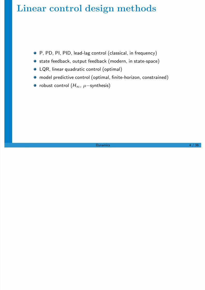
Linear control design methods
P, PD, PI, PID, lead-lag control (classical, in frequency)
state feedback, output feedback (modern, in state-space)
LQR, linear quadratic control (optimal)model predictive control (optimal, finite-horizon, constrained)
robust control (H ∞, µ−synthesis)
M. Mazo Jr. (DCSC/TUD) Dynamics 4 / 36
7/25/2019 Hyu 01213
http://slidepdf.com/reader/full/hyu-01213 5/36
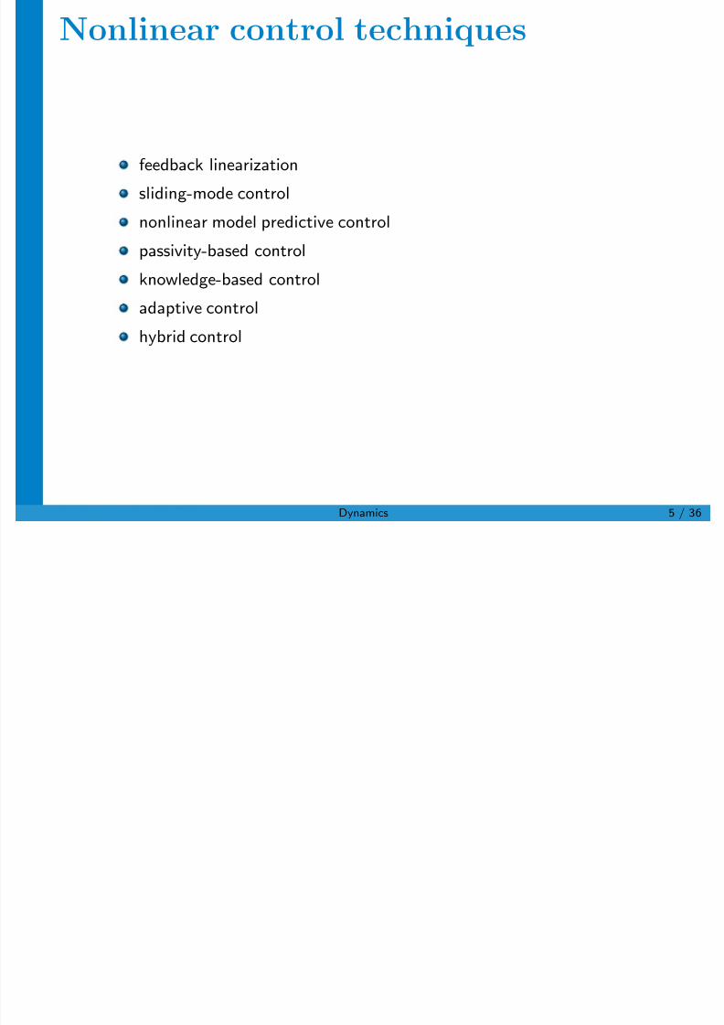
Nonlinear control techniques
feedback linearization
sliding-mode control
nonlinear model predictive control
passivity-based control
knowledge-based control
adaptive control
hybrid control
M. Mazo Jr. (DCSC/TUD) Dynamics 5 / 36
7/25/2019 Hyu 01213
http://slidepdf.com/reader/full/hyu-01213 6/36
Outline
1 Overview of control design methods
2 Continuous vs. discrete time design
3 State-feedback control, observers
4 Control architectures, nonlinear control
5 PID controllers
M. Mazo Jr. (DCSC/TUD) Dynamics 6 / 36
7/25/2019 Hyu 01213
http://slidepdf.com/reader/full/hyu-01213 7/36
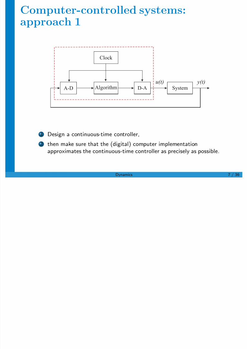
Computer-controlled systems:approach 1
y(t)u(t)Algorithm
Clock
A-D D-A System
1 Design a continuous-time controller,
2 then make sure that the (digital) computer implementationapproximates the continuous-time controller as precisely as possible.
M. Mazo Jr. (DCSC/TUD) Dynamics 7 / 36

7/25/2019 Hyu 01213
http://slidepdf.com/reader/full/hyu-01213 8/36
Computer-controlled systems:approach 2
y(t)u(t)Algorithm
Clock
A-D D-A System
1 Describe the system from the computer’s (digital) viewpoint,
2 and design directly a discrete-time controller.
M. Mazo Jr. (DCSC/TUD) Dynamics 8 / 36
7/25/2019 Hyu 01213
http://slidepdf.com/reader/full/hyu-01213 9/36
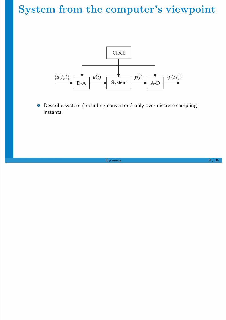
System from the computer’s viewpoint
y t ( )u t ( )System
Clock
{ ( )} y t k { ( )}u t k A-DD-A
Describe system (including converters) only over discrete sampling
instants.
M. Mazo Jr. (DCSC/TUD) Dynamics 9 / 36
7/25/2019 Hyu 01213
http://slidepdf.com/reader/full/hyu-01213 10/36
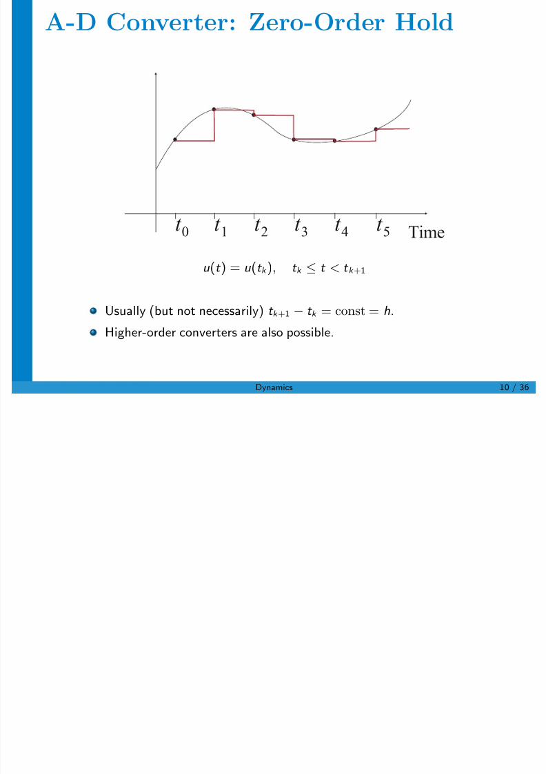
A-D Converter: Zero-Order Hold
Timet t t t t t
0 1 2 3 4 5
u (t ) = u (t k ), t k ≤ t < t k +1
Usually (but not necessarily) t k +1 − t k = const = h.
Higher-order converters are also possible.
M. Mazo Jr. (DCSC/TUD) Dynamics 10 / 36
7/25/2019 Hyu 01213
http://slidepdf.com/reader/full/hyu-01213 11/36
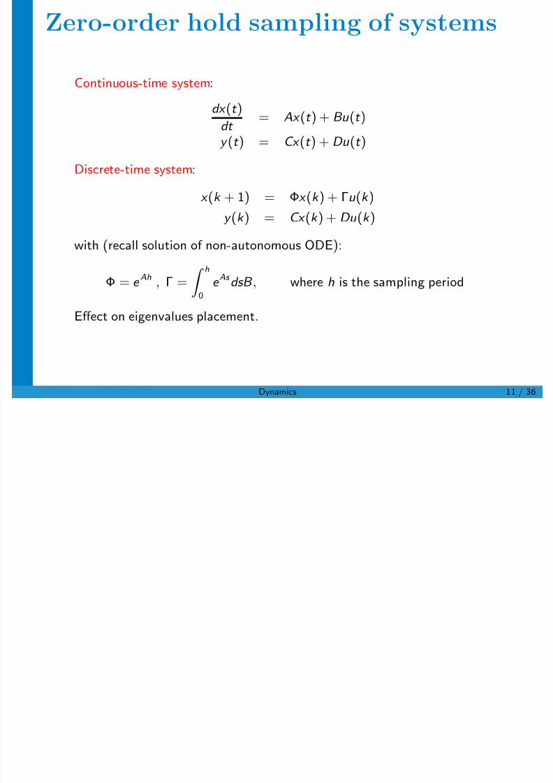
Zero-order hold sampling of systems
Continuous-time system:
dx (t )
dt = Ax (t ) + Bu (t )
y (t ) = Cx (t ) + Du (t )
Discrete-time system:
x (k + 1) = Φx (k ) + Γu (k )
y (k ) = Cx (k ) + Du (k )
with (recall solution of non-autonomous ODE):
Φ = e Ah
, Γ = h
0e As
dsB , where h is the sampling period
Effect on eigenvalues placement.
M. Mazo Jr. (DCSC/TUD) Dynamics 11 / 36
7/25/2019 Hyu 01213
http://slidepdf.com/reader/full/hyu-01213 12/36
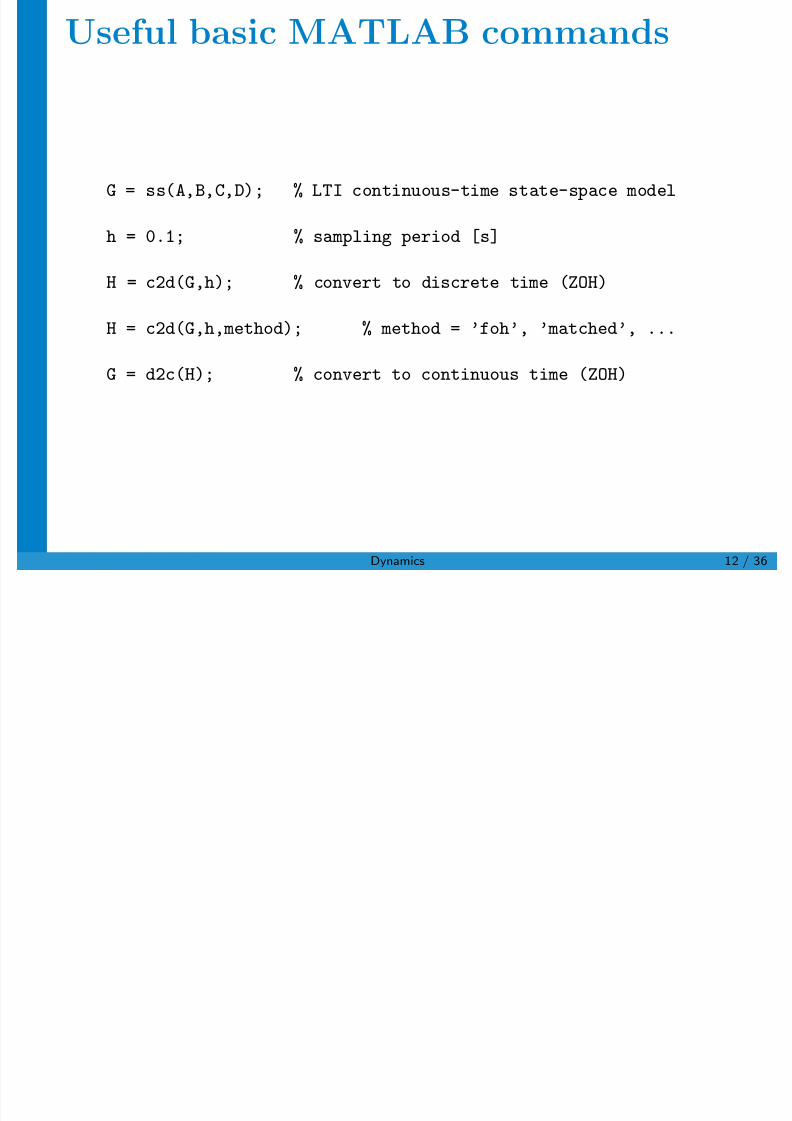
Useful basic MATLAB commands
G = ss(A,B,C,D); % LTI continuous-time state-space model
h = 0.1; % sampling period [s]
H = c2d(G,h); % convert to discrete time (ZOH)
H = c2d(G,h,method); % method = ’foh’, ’matched’, ...
G = d2c(H); % convert to continuous time (ZOH)
M. Mazo Jr. (DCSC/TUD) Dynamics 12 / 36
7/25/2019 Hyu 01213
http://slidepdf.com/reader/full/hyu-01213 13/36
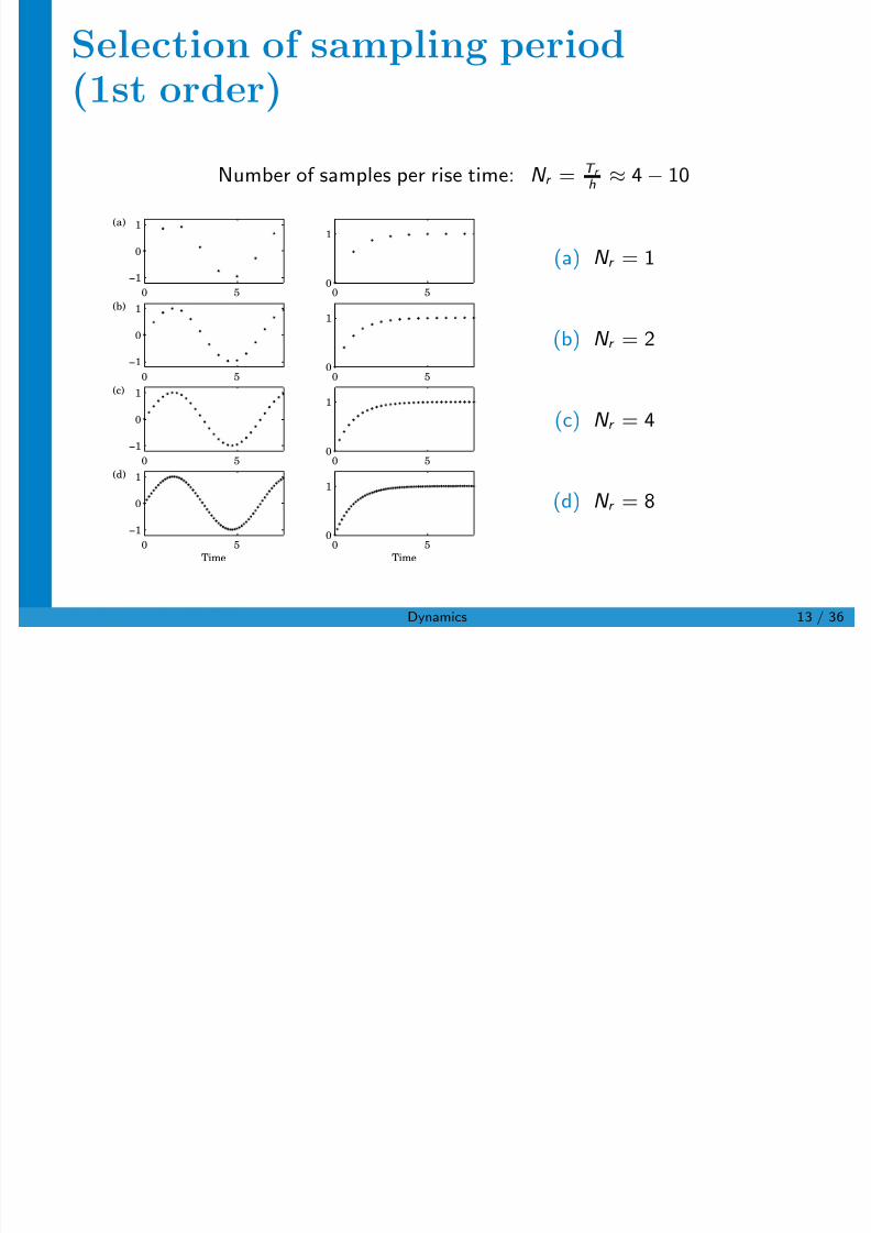
Selection of sampling period(1st order)
Number of samples per rise time: N r = T r h ≈ 4− 10
0 5
−1
0
1(a)
0 50
1
0 5
−1
0
1(b)
0 50
1
0 5
−1
0
1(c)
0 50
1
0 5
−1
0
1(d)
Time
0 50
1
Time
(a) N r = 1
(b) N r = 2
(c) N r = 4
(d) N r = 8
M. Mazo Jr. (DCSC/TUD) Dynamics 13 / 36
7/25/2019 Hyu 01213
http://slidepdf.com/reader/full/hyu-01213 14/36
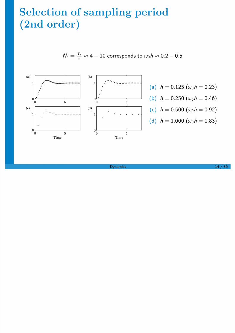
Selection of sampling period(2nd order)
N r = T r h ≈ 4− 10 corresponds to ω0h ≈ 0.2− 0.5
0 50
1
(a)
0 50
1
(b)
0 50
1
(c)
Time
0 50
1
(d)
Time
(a) h = 0.125 (ω0h = 0.23)
(b) h = 0.250 (ω0h = 0.46)
(c) h = 0.500 (ω0h = 0.92)
(d) h = 1.000 (ω0h = 1.83)
M. Mazo Jr. (DCSC/TUD) Dynamics 14 / 36
7/25/2019 Hyu 01213
http://slidepdf.com/reader/full/hyu-01213 15/36
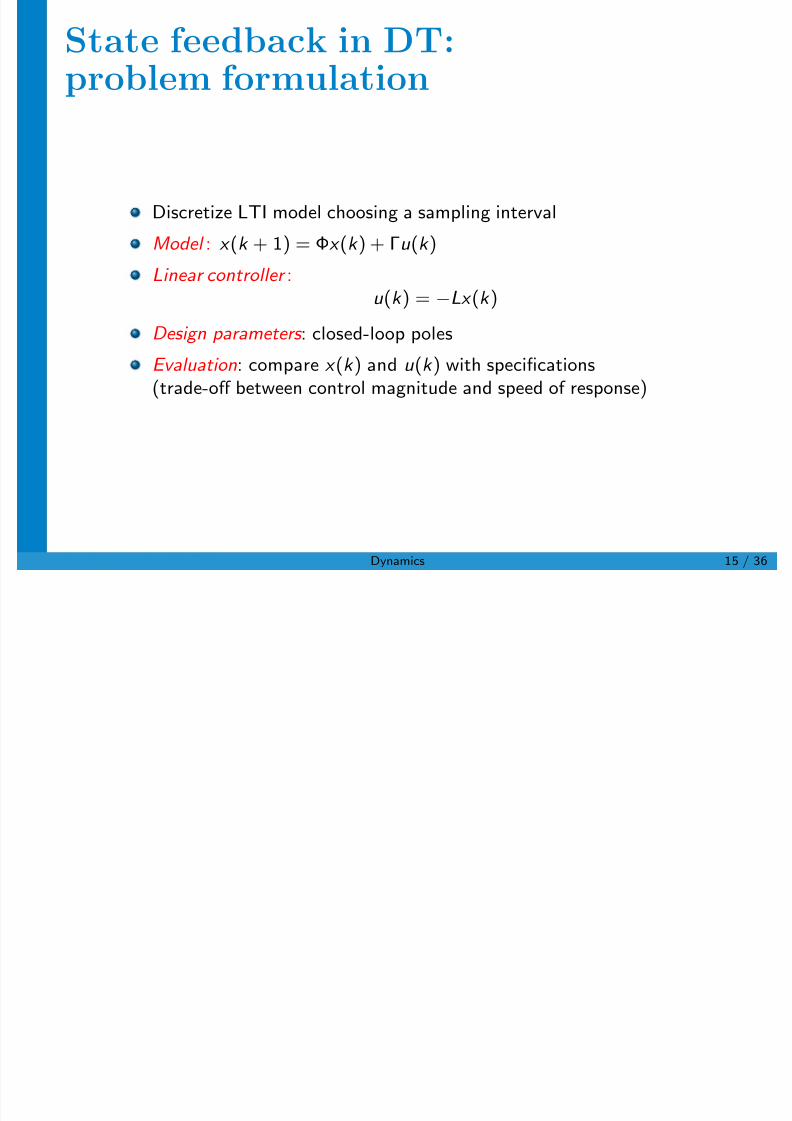
State feedback in DT:problem formulation
Discretize LTI model choosing a sampling interval
Model : x (k + 1) = Φx (k ) + Γu (k )
Linear controller :u (k ) = −Lx (k )
Design parameters : closed-loop poles
Evaluation: compare x (k ) and u (k ) with specifications(trade-off between control magnitude and speed of response)
M. Mazo Jr. (DCSC/TUD) Dynamics 15 / 36
P l l A k ’ f l
7/25/2019 Hyu 01213
http://slidepdf.com/reader/full/hyu-01213 16/36
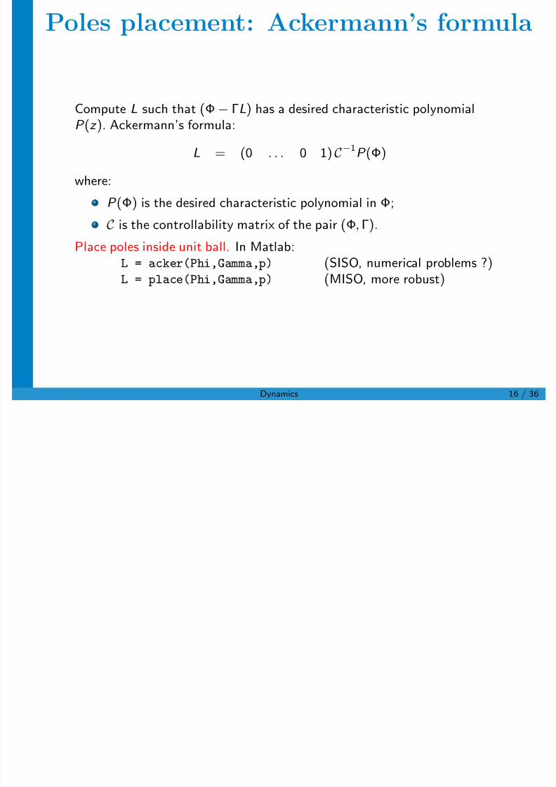
Poles placement: Ackermann’s formula
Compute L such that (Φ − ΓL) has a desired characteristic polynomialP (z ). Ackermann’s formula:
L = (0 . . . 0 1) C −1P (Φ)
where:
P (Φ) is the desired characteristic polynomial in Φ;
C is the controllability matrix of the pair (Φ, Γ).
Place poles inside unit ball. In Matlab:L = acker(Phi,Gamma,p) (SISO, numerical problems ?)
L = place(Phi,Gamma,p) (MISO, more robust)
M. Mazo Jr. (DCSC/TUD) Dynamics 16 / 36
Alt ti l h th d i d l
7/25/2019 Hyu 01213
http://slidepdf.com/reader/full/hyu-01213 17/36
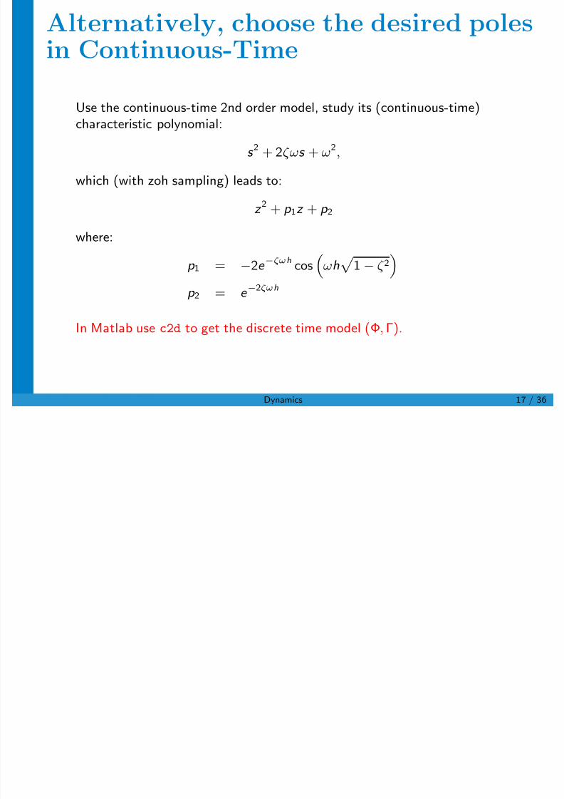
Alternatively, choose the desired polesin Continuous-Time
Use the continuous-time 2nd order model, study its (continuous-time)characteristic polynomial:
s 2 + 2ζωs + ω2,
which (with zoh sampling) leads to:
z 2 + p 1z + p 2
where:
p 1 = −2e −ζωh cos
ωh
1− ζ 2
p 2 = e −2ζωh
In Matlab use c2d to get the discrete time model (Φ,Γ).
M. Mazo Jr. (DCSC/TUD) Dynamics 17 / 36
Li d ti t l LQR
7/25/2019 Hyu 01213
http://slidepdf.com/reader/full/hyu-01213 18/36
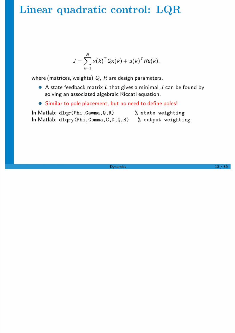
Linear quadratic control: LQR
J =N
k =1
x (k )T Qx (k ) + u (k )T Ru (k ),
where (matrices, weights) Q
, R
are design parameters.A state feedback matrix L that gives a minimal J can be found bysolving an associated algebraic Riccati equation.
Similar to pole placement, but no need to define poles!
In Matlab: dlqr(Phi,Gamma,Q,R) % state weighting
In Matlab: dlqry(Phi,Gamma,C,D,Q,R) % output weighting
M. Mazo Jr. (DCSC/TUD) Dynamics 18 / 36
O tli
7/25/2019 Hyu 01213
http://slidepdf.com/reader/full/hyu-01213 19/36
Outline
1 Overview of control design methods
2 Continuous vs. discrete time design
3 State-feedback control, observers
4 Control architectures, nonlinear control
5 PID controllers
M. Mazo Jr. (DCSC/TUD) Dynamics 19 / 36
St t ti ti b
7/25/2019 Hyu 01213
http://slidepdf.com/reader/full/hyu-01213 20/36
State estimation: observers
x (k + 1) = Φx (k ) + Γu (k )
y (k ) = Cx (k )
Assume input and output are available, reconstruct the state:
Direct calculation;Luenberger observer (model-based);
Kalman filter (optimal in presence of Gaussian noise).
Note: the terms “observer”, “estimator”, “filter” are in this context usedsynonymously.
M. Mazo Jr. (DCSC/TUD) Dynamics 20 / 36
M del b ed e ti ti
7/25/2019 Hyu 01213
http://slidepdf.com/reader/full/hyu-01213 21/36
Model-based estimation
1 Consider the model:
x (k + 1) = Φx (k ) + Γu (k )
2 Introduce ”feedback” from measured y (k )
x (k + 1) = Φx (k ) + Γu (k ) + K [y (k )− C x (k )]
3 Define the estimation error e = x − x
e (k + 1) = Φe (k )− KCe (k ) = [Φ− KC ]e (k )
M. Mazo Jr. (DCSC/TUD) Dynamics 21 / 36
Observer block diagram
7/25/2019 Hyu 01213
http://slidepdf.com/reader/full/hyu-01213 22/36
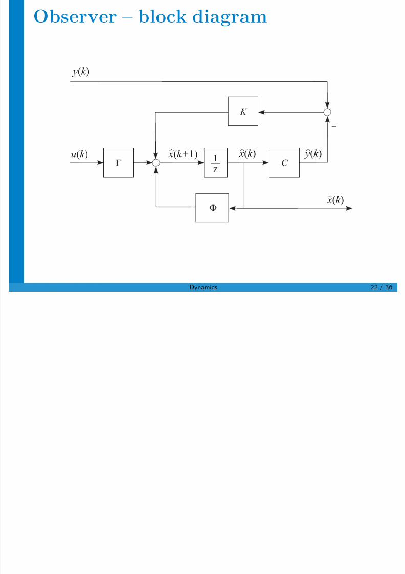
Observer – block diagram
K
1z
u k ( ) x k+( 1)^ y k ( )^
y k ( )
C x k ( )^
x k ( )^
M. Mazo Jr. (DCSC/TUD) Dynamics 22 / 36
Output feedback (observer + state
7/25/2019 Hyu 01213
http://slidepdf.com/reader/full/hyu-01213 23/36
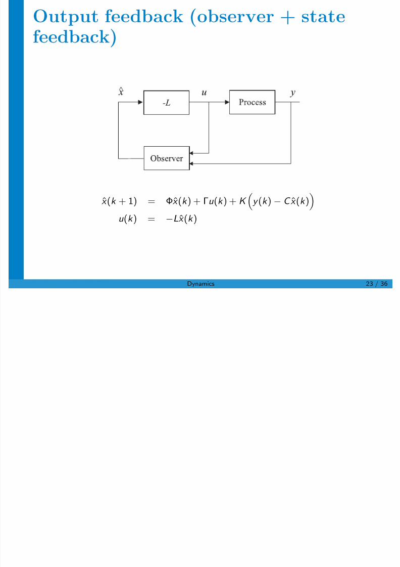
Output feedback (observer + statefeedback)
ˆx
(k
+ 1) = Φˆx
(k
) + Γu
(k
) + K y
(k
)− C
ˆx
(k
)
u (k ) = −Lx (k )
M. Mazo Jr. (DCSC/TUD) Dynamics 23 / 36
Poles of the closed loop system
7/25/2019 Hyu 01213
http://slidepdf.com/reader/full/hyu-01213 24/36
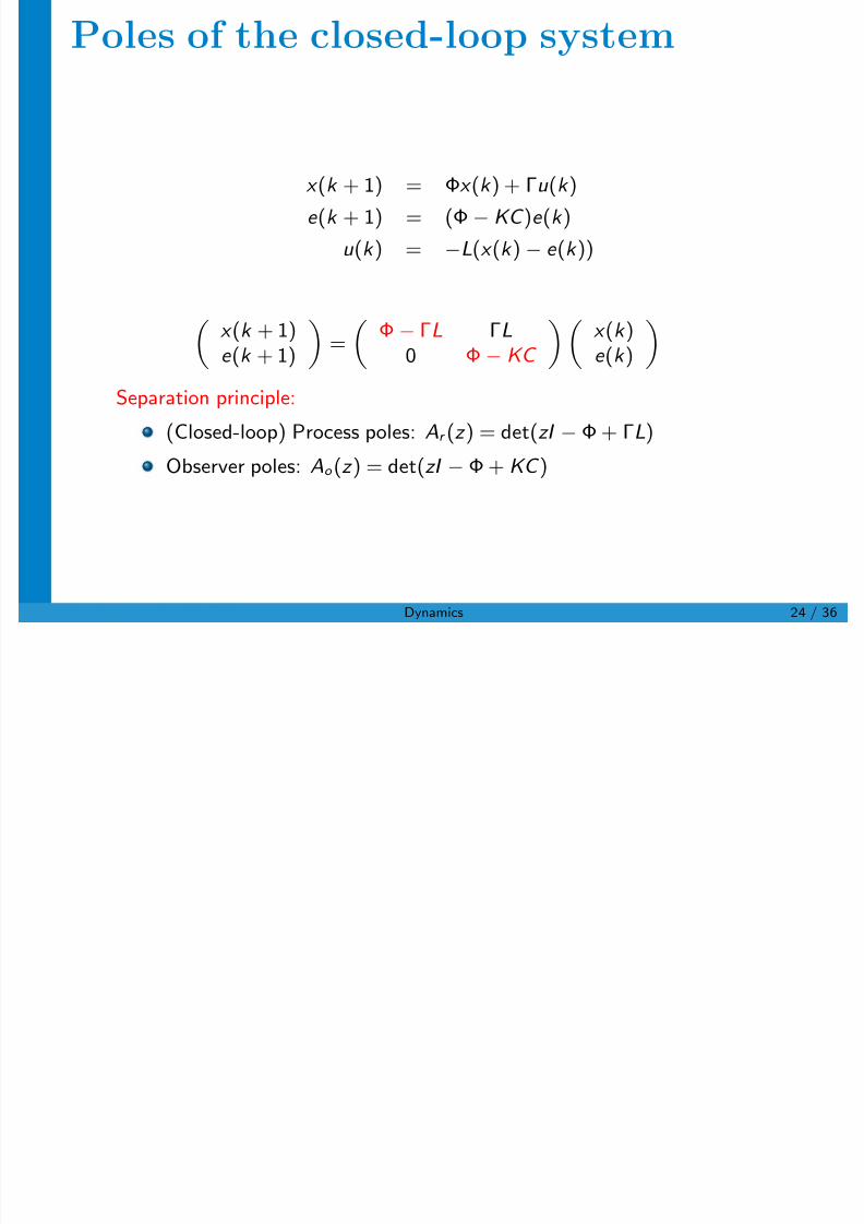
Poles of the closed-loop system
x (k + 1) = Φx (k ) + Γu (k )
e (k + 1) = (Φ− KC )e (k )
u (k ) = −L(x (k )− e (k ))
x (k + 1)
e (k + 1)
=
Φ− ΓL ΓL
0 Φ− KC
x (k )
e (k )
Separation principle:
(Closed-loop) Process poles: Ar (z ) = det(zI − Φ + ΓL)
Observer poles: Ao (z ) = det(zI − Φ + KC )
M. Mazo Jr. (DCSC/TUD) Dynamics 24 / 36
Outline

7/25/2019 Hyu 01213
http://slidepdf.com/reader/full/hyu-01213 25/36
Outline
1 Overview of control design methods
2 Continuous vs. discrete time design
3 State-feedback control, observers
4 Control architectures, nonlinear control
5 PID controllers
M. Mazo Jr. (DCSC/TUD) Dynamics 25 / 36
Feed-forward (two-degree-of-freedom)
7/25/2019 Hyu 01213
http://slidepdf.com/reader/full/hyu-01213 26/36
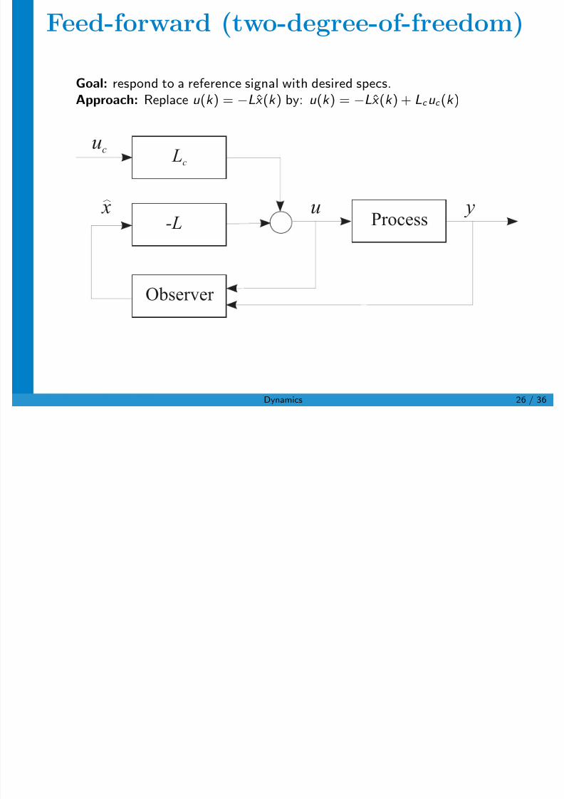
Feed-forward (two-degree-of-freedom)
Goal: respond to a reference signal with desired specs.
Approach: Replace u (k ) = −Lx (k ) by: u (k ) = −Lx (k ) + Lc u c (k )
u x^
Lc
Observer
Process-L
uc
y
M. Mazo Jr. (DCSC/TUD) Dynamics 26 / 36
Feed-forward (two-degree-of-freedom)
7/25/2019 Hyu 01213
http://slidepdf.com/reader/full/hyu-01213 27/36
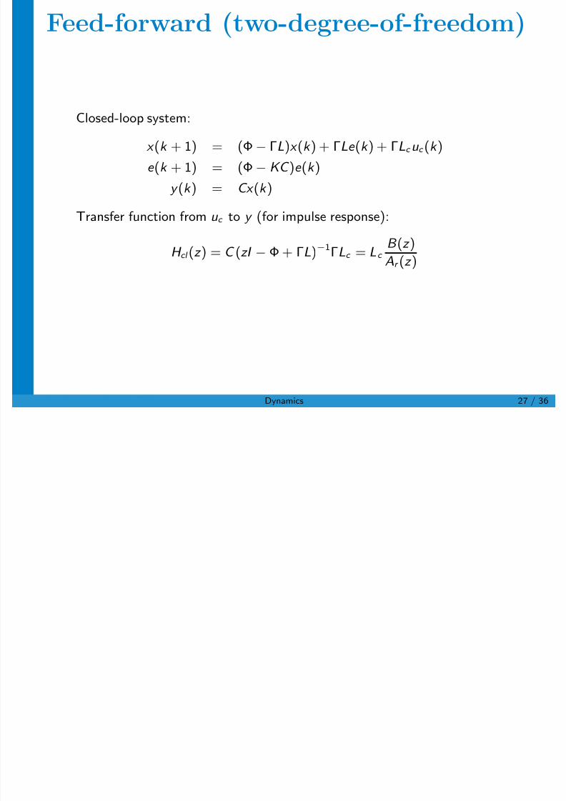
Feed-forward (two-degree-of-freedom)
Closed-loop system:
x (k + 1) = (Φ− ΓL)x (k ) + ΓLe (k ) + ΓLc u c (k )
e (k + 1) = (Φ− KC )e (k )
y (k ) = Cx (k )
Transfer function from u c to y (for impulse response):
H cl (z ) = C (zI − Φ + ΓL)−1ΓLc = Lc
B (z )
Ar (z )
M. Mazo Jr. (DCSC/TUD) Dynamics 27 / 36
Application to a nonlinear system
7/25/2019 Hyu 01213
http://slidepdf.com/reader/full/hyu-01213 28/36
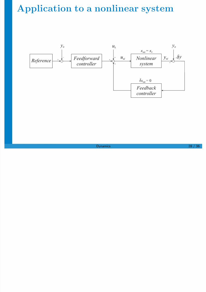
Application to a nonlinear system
Feedback controller
Reference Nonlinear
system
y0
y
u0
y0
Feedforward controller
δ
δ
M. Mazo Jr. (DCSC/TUD) Dynamics 28 / 36
Control by local linear controller
7/25/2019 Hyu 01213
http://slidepdf.com/reader/full/hyu-01213 29/36
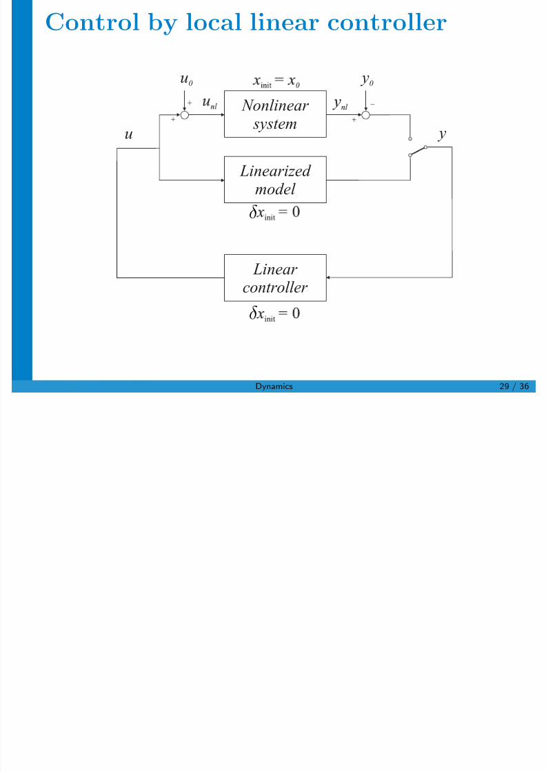
Control by local linear controller
u
u0
Linear
controller
Nonlinear system
y0
y
Linearized
model
δ
δ
M. Mazo Jr. (DCSC/TUD) Dynamics 29 / 36
Model-based adaptive control
7/25/2019 Hyu 01213
http://slidepdf.com/reader/full/hyu-01213 30/36
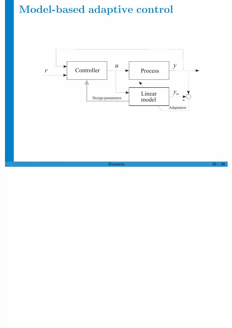
Model based adaptive control
u
Adaptation
Design parameters
Controller
-
Process
Linear model
yr
ym
M. Mazo Jr. (DCSC/TUD) Dynamics 30 / 36
Outline
7/25/2019 Hyu 01213
http://slidepdf.com/reader/full/hyu-01213 31/36
Outline
1 Overview of control design methods
2 Continuous vs. discrete time design
3 State-feedback control, observers
4 Control architectures, nonlinear control
5 PID controllers
M. Mazo Jr. (DCSC/TUD) Dynamics 31 / 36
Continuous-time PID controller
7/25/2019 Hyu 01213
http://slidepdf.com/reader/full/hyu-01213 32/36
Continuous time PID controller
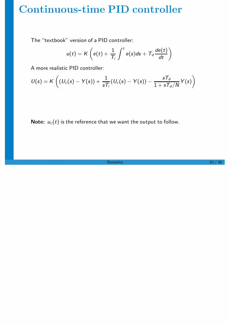
The “textbook” version of a PID controller:
u (t ) = K
e (t ) +
1
T i
t e (s )ds + T d
de (t )
dt
A more realistic PID controller:
U (s ) = K
(U c (s )− Y (s )) + 1sT i
(U c (s )− Y (s ))− sT d 1 + sT d /N Y (s )
Note: u c (t ) is the reference that we want the output to follow.
M. Mazo Jr. (DCSC/TUD) Dynamics 32 / 36
Discrete-time PID controller
7/25/2019 Hyu 01213
http://slidepdf.com/reader/full/hyu-01213 33/36
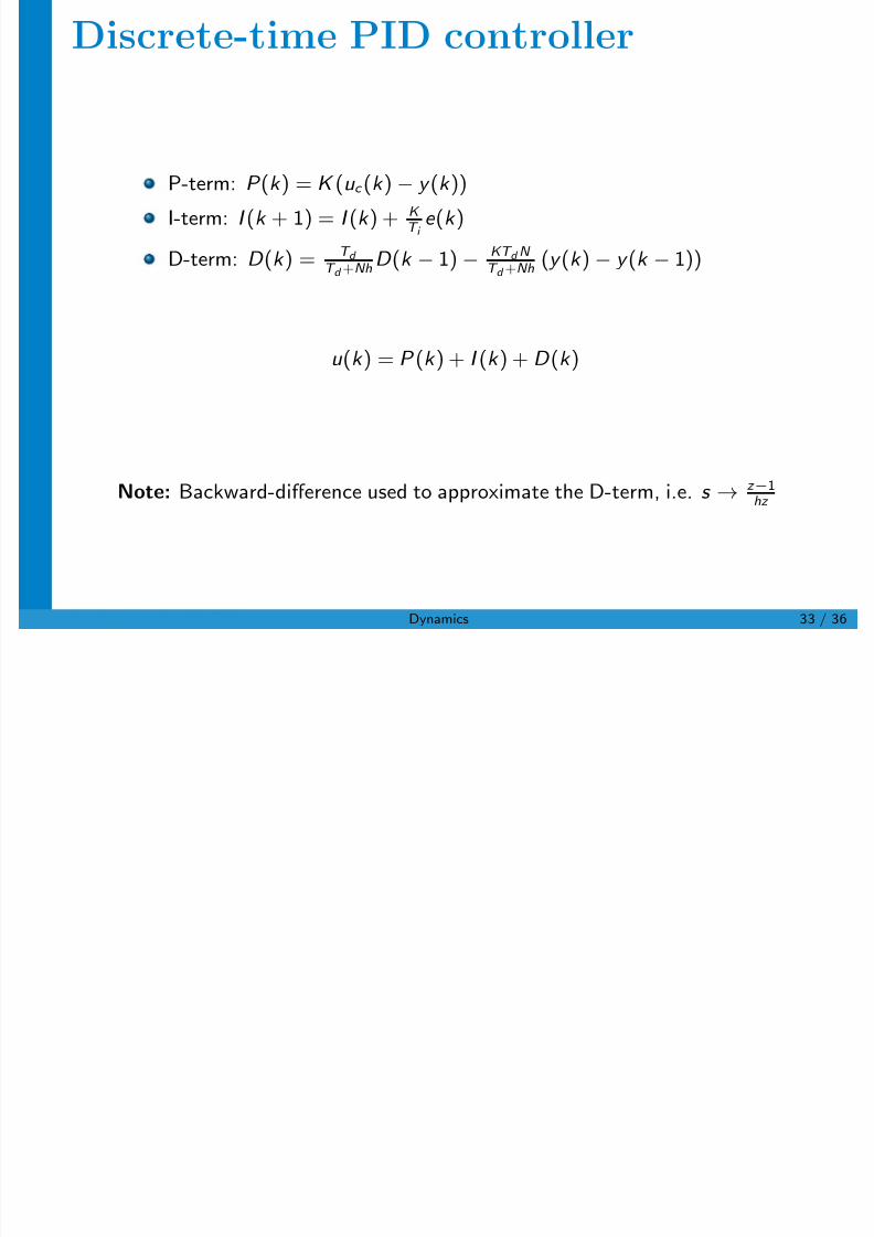
P-term: P (k ) = K (u c (k )− y (k ))
I-term: I (k + 1) = I (k ) + K
T i e (k )
D-term: D (k ) = T d T d +Nh
D (k − 1)− KT d N
T d +Nh (y (k )− y (k − 1))
u (k ) = P (k ) + I (k ) + D (k )
Note: Backward-difference used to approximate the D-term, i.e. s → z −1hz
M. Mazo Jr. (DCSC/TUD) Dynamics 33 / 36
PID tuning
7/25/2019 Hyu 01213
http://slidepdf.com/reader/full/hyu-01213 34/36
g
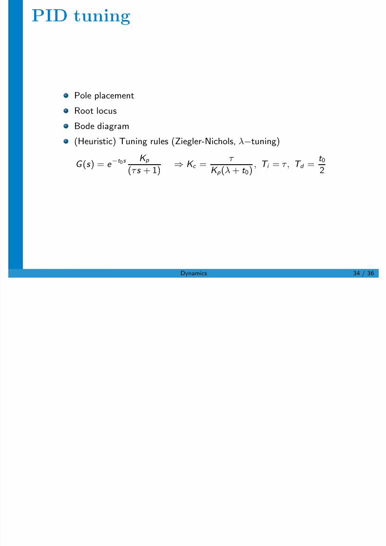
Pole placement
Root locus
Bode diagram
(Heuristic) Tuning rules (Ziegler-Nichols, λ−tuning)
G (s ) = e −t 0s
K p
(τ s + 1) ⇒ K c =
τ
K p (λ + t 0), T i = τ , T d =
t 0
2
M. Mazo Jr. (DCSC/TUD) Dynamics 34 / 36
Example of a complete controller:
7/25/2019 Hyu 01213
http://slidepdf.com/reader/full/hyu-01213 35/36
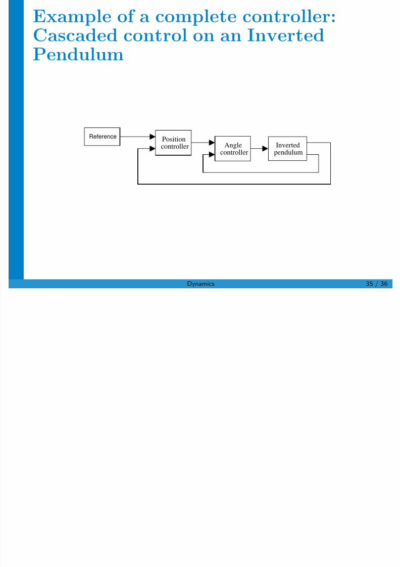
p pCascaded control on an InvertedPendulum
Reference
Position controller Inverted pendulum
Angle controller
M. Mazo Jr. (DCSC/TUD) Dynamics 35 / 36
The End

7/25/2019 Hyu 01213
http://slidepdf.com/reader/full/hyu-01213 36/36
Thanks for your attention!Questions?
M. Mazo Jr. (DCSC/TUD) Dynamics 36 / 36


![· -./01213&4567 89:);?@AB C0DE)FGHIJK7L,M NO’P:QR1S;TDU& VW XYZ[\]^_-‘56 abcde) fFGHIghi7 Ljk)Xlme ‘5noopq rs)tu^v)wxyz{|} ~ ‘56&•†‡…7](https://img.pdfslide.net/doc/110x75/5fb9cdb365bf7b40c512d390/-012134567-89ab-c0defghijk7lm-noapqr1stdu-vw-xyz-a56.jpg)