I. Introduction

A textbook consequence of competitive markets is that an industry-wide increase in the

price of inputs will be passed on to consumers through an increase in prices. This fundamental

implication has been explored by researchers interested in who bears the burden of taxation and

exchange rate fluctuations. However, little attention has focused on the price implications of

minimum wage hikes. From a policy perspective, this is an oversight. Welfare analysis of

minimum wage laws should not ignore consumers. Furthermore, estimates of price shifting can

have important implications for wage-push inflation stories, as well as potentially provide an

explanation for the small short-run employment effects that have been found in some of the

minimum wage literature.

The only work that explores minimum wage price shifting is Card and Krueger (1995),

who collected price information from respondent restaurants in their research on fast food

restaurants. Their results are mixed and difficult to interpret due to the imprecision of many of

their estimates. Generally, they find little evidence of price inflation in their Texas fast food

restaurant sample but more, yet still mixed, evidence from their New Jersey-Pennsylvania sample.

However, this work is limited to restaurants in three states and two minimum wage episodes.

Other work that they present looks at a broader cross-sectional sample of U.S. states but is also

limited to the period surrounding the early 1990s federal increases.

This paper uses several data sources on restaurant prices to more thoroughly examine the

impact of minimum wage hikes in Canada and the U.S. Particular attention is paid to the timing

of these price changes and their overall impact relative to full or competitive price pass-through

predictions. Section II briefly describes the price implications of minimum wage hikes, including

the predicted elasticity that would be consistent with full price shifting. Three data sources on

prices are described in section III. Section IV presents the empirical strategy and results. The

results suggest that restaurant prices rise roughly one-for-one with increases in the wage bill that

result from minimum wage legislation. Furthermore, the price responses are concentrated in the

2

quarter surrounding the month that the legislation is enacted. Although minimum wage legislation

is typically enacted many months in advance, there is no price response leading up to the hike and

little adjustment in the months subsequent to the hike, excepting the few months around the

enactment date. If anything, there is some evidence that minimum wage price effects dissipate

over time. The magnitude of these findings is roughly the same in the U.S. and Canada, and is

fairly robust to changes in data, specification, and estimation techniques. However, because of

small predicted elasticities, it is difficult to draw inferences about the price impact on broader

indices or industries that have a small share of low wage labor.

II. The Price Effect of a Minimum Wage Increase

While there has been little work on the price impact of minimum wage increases, there is a

literature on the price response to changes in other industry-wide costs, such as sales taxes and

exchange rates.1 In the standard perfect competition analysis, assuming constant marginal cost

and demand elasticity, an increase in the price of an input is fully shifted to consumers. This

implication arises from many models, but can be easily seen by looking at the comparative statics

from a conjectural variations model, where the firm chooses an output xi to maximize

(1) q X xi C xi xi( ) ( )− − δ .

q(X) is the inverse demand function for the industry, X is total industry output, C( xi ) is the

industry cost of production, and δ is the additional cost of labor due to minimum wage laws.

The interpretation of δ is discussed below. The first order condition for a profit maximizer is

(2) q X q X xi Cxiq X xi i( ) ( ) ( )+ ′ − − + ′ =δ α 0

1 On taxes, see Sumner (1981), Sullivan (1985), Katz and Rosen (1985), Karp and Perloff (1989), Besley andRosen (1994), and Poterba (1996). The latter two papers describe the literature. Recent examples of exchange-ratepassthrough include Gron and Swenson (1996), Lee (1997) and Yang (1997).

where α i dX dxi= / is the firm i's conjectural variation or the amount by which a one unit

change in firm i's output will affect total industry output. Differentiating (2), it can be shown that

3

the impact of an industry-wide cost change on price depends critically on industry market

structure (α i ) and demand elasticities (ε ):

(3)dqd

q Xxi

iN

δ∂∂δ= ′ =∑( ) 1

where ∂∂δ α ε αxi

i i Cxi xiq

= − + + − ′1

2 1( ) / and ε = −

′′′

xiq

q

and N is the number of firms in the industry. In the simple case of linear costs ( Cxixiq/ ′= 0 )

and a perfectly competitive market (α i = − 1), firms set output at a level at which price is equal to

marginal cost. Changes in the minimum wage are fully passed on to the consumer.

However, more generally, the degree of shifting depends on a variety of factors, including

the magnitude of the demand elasticity, the convexity of demand, the elasticity of marginal cost

with respect to output, and the degree of competition. These findings have been generalized by

Stern (1987), Besley (1989), and Delipalla and Keen (1992) to allow for free entry and various

cost structures. They show that, under specific conditions, even overshifting can occur in

imperfectly competitive markets.2 Undershifting is more commonly observed, reflecting the

elastic demand of many products. For example, Yang (1997) shows that product differentiation

plays a key role in partial pass-through of exchange rate fluctuations, suggesting that pass-through

is generally smaller with products that have a high degree of substitutability. Furthermore,

industry demand and supply conditions may lead to dynamic issues about the difference between

long and short run responses. For example, on the supply side, prices may not react

instantaneously to cost changes.3 Gron and Swenson (1996) find that automobile producers

transfer their production across national borders to deal with exchange rate fluctuations, leading

to undershifting of prices relative to exchange rate movements. In a similar vein, undershifting of

2 Empirically, overshifting of ad valorem taxes has been found by, among others, Besley and Rosen (1994) in theretail apparel industry and Karp and Perloff (1989) in the Japanese television market.3 See Ball and Mankiw (1994) on sticky prices.

4

minimum wage hikes can occur if consumers cross state borders to purchase goods. Therefore,

empirically, it is not surprising that pass-through predictions vary across industries and, even

within industries, across studies. As a result, the impact of an industry-wide cost change, such as

a minimum wage hike, on price behavior is very much an empirical issue.

What is the Full Price Pass-Through Prediction?

Further confounding the measurement of the extent of price shifting from minimum wage

legislation is that the full shifting amount must be estimated. In the simplest case, a competitive

market with inverse demand function q=q(Y) and all firms facing the same constant returns to

scale production technology, an increase in the wage increases the industry's selling price by the

affected labor's share of operating cost. Assume affected labor is computed as the product of the

share of labor cost (L) in total operating cost (C) and the fraction of workers that are affected by

the minimum wage level ( Emw E/ ). The increase in wages will lead to an increase in prices that

is proportional to the share of affected labor:

(4) δ=−

LC

EmwE

wtwt 1

However, Equation (4) ignores two factors. First, demand may fall when restaurants raise

prices, thus biasing upward the full pass-through prediction of (4).4 But in the case of

industry-wide price shifts, such as when the minimum wage increases, the relevant output

elasticity is the industry's, which is likely to be much smaller than any individual restaurant's

elasticity. Brown (1990) estimates that the price elasticity of demand for all restaurants is -0.2 but

is -1.0 for fast food restaurants. Therefore, the relatively inelastic demand for restaurant food

suggests that the output bias to (4) is likely to be small for restaurants but may be problematic for

fast food products.

4 Partly counterbalancing this effect is the possibility that workers whose wages are increased by a minimum wagehike increase their demand for restaurant products.

5

Second, equation (4) does not take into account the possibility that firms substitute capital

or high wage labor for low wage labor when minimum wages increase. However, consistent with

Shephard's lemma, this bias is likely to be negligible. Evidence on this proposition is exemplified

by the contentious literature on employment effects of minimum wage increases. This debate

seems to revolve around whether there is a small effect (Neumark and Wascher 1992) or no effect

(Card and Krueger 1995) of minimum wage increases on low wage employment. Even using

Neumark and Wascher's employment elasticity does not substantially alter the estimate of δ. In

addition, to quantify the importance of capital-labor substitution bias, I computed labor shares

(L/C) from McDonald's annual reports for 1988 to 1995. For this specific company, the share of

labor does not change, despite two federal minimum wage increases and 28 state increases. In

1988, labor share is 31.1 percent of company-operated expenses and in 1995 it is 31.2 percent.

Between 1989 and 1992 (encompassing two federal increases that raised the nominal minimum

wage by 27%), labor share remained constant at 31.1 percent. Of course, this particular evidence

does not allow us to preclude the possibility that McDonald's shifts labor costs away from low

wage workers and toward higher wage workers in response to minimum wage increases.

Therefore, while I am confident that using equation (4) will closely approximate the full shifting

minimum wage price elasticity, the actual pass-through prediction, which is detailed next, should

be considered an upper bound estimate.

Labor Share in the Restaurant Industry

To compute labor share in the restaurant industry, two data sources are employed. First, I

searched the SEC's EDGAR database of annual and quarterly company reports using five

keywords: restaurant, steak, seafood, hamburger, and chicken. Of the 17 restaurant companies

that appeared, the mean and median 1995 payroll expense to total cost ratio is approximately 30

percent, roughly consistent with McDonald's payroll to expense ratio of 31 percent.5

5 The standard deviation is 5.0 percent, the minimum is 20.7 percent (Food Quest), and the maximum is 41.7percent (Cooker Restaurants).

6

Second, the Internal Revenue Service summarizes operating costs by industry in the

Statistics on Income Bulletin. This data come from a sampling of corporate income tax forms.

Because operating costs are broken down by category, it is possible to calculate labor share.6

Unfortunately, I must look at partnerships rather than corporations because, according to

communication with the IRS, labor cost is notoriously difficult to decompose for corporations.

The IRS analysts do not believe this is a serious problem for smaller firms. Nevertheless, the

figure reported in the IRS sample is roughly the same as in the SEC sample; the labor share of

operating costs among eating place partnerships is 33 percent. The labor share for all industries is

19 percent.

The Fraction of Minimum Wage Workers in the Restaurant Industry

Estimating Emw/E is more precarious. The primary complication arises because the

minimum wage may have a spillover effect on the wage distribution (Grossman 1983, Card and

Krueger 1995, and Green and Paarsch 1997).7 In particular, Card and Krueger estimate that

approximately 33 to 40 percent of Texas fast food restaurants increased the wage of workers who

were already above the old minimum (but below the new minimum) to a level beyond the new

minimum after the new law took effect. As for workers already well above the new minimum

wage, only nine percent of restaurants with a starting wage equal to the minimum increased the

pay of their high-wage workers. However, 60 percent that start their employees at a much higher

level bumped up their employees to maintain a wage differential from other restaurants.

To calculate the fraction of the restaurant population affected by a minimum wage hike, I

use the March rotation of the 1986 to 1993 Current Population Surveys. Table 1 reports some of

the findings. The top row reports the fraction of workers in four industry classifications - all

6 Labor cost is the sum of wages and salaries, cost of labor in the cost of sales and operations, employee benefitplans, half of repairs, and pension, profit sharing, and other annuities. Total operating cost is the sum of cost ofsales and operations, rent, interest, taxes, bad debts, repairs, depreciation, depletion, guaranteed payments topartners, wages and salaries, employee benefit plans, and pension, profit sharing, and other annuities.7 Workers above the new minimum may get raises because of shifts in demand away from unskilled and towardskilled workers after a minimum wage increase. Grossman (1983) presents an alternative model that relies on acorrelation between skilled worker effort and the difference between skilled and unskilled wages.

7

private, retail trade, restaurant, and food service workers -- who are at or below their state's

minimum wage (columns 1 to 4) or above but within one dollar of the minimum wage level

(columns 5 to 8). Hourly earnings, which includes tips, is defined as weekly earnings divided by

weekly hours. Approximately 24 percent of all restaurant employees in the U.S. are at or below

the minimum wage and an additional 37 percent are within one dollar. When the sample includes

only those who are in food service, about 29 percent are at or below the minimum and an

additional 40 percent are within one dollar. However, these numbers vary dramatically across

states. Very few workers earn the minimum wage in Alaska, even though state law requires the

minimum to be 50 cents above the federal threshold. However, in West Virginia, over one-half of

all food service workers are at the minimum wage and close to 90 percent are within one dollar.

The figures are somewhat similar when using fraction of total hours worked by low wage

workers; the slightly smaller numbers account for the fewer hours worked by low wage workers.

Consequently, using equation (4), a one percent increase in the minimum wage level will

increase restaurant prices by 0.11 percent when additional labor costs are fully passed through to

consumers. This figure assumes that all workers below and one-third of workers within one

dollar of the new minimum wage have their pay increased by the same amount as a result of a

minimum wage change, and there are no additional effects from a change in the price of

intermediate goods. If only minimum wage workers are affected by an increase, the full price

shifting elasticity is 0.075. The corresponding elasticity for broader CPI measures is substantially

smaller; the predicted pass-through is in the order of 0.015 to 0.020, reflecting that five percent of

private industry workers are below the minimum wage, an additional 10 percent are within one

dollar, and labor share is roughly 20 percent for all industries.8 However, these elasticities are

best considered upper bound estimates because of the possibility of output and substitution biases.

8 It would be interesting to analyze other industries, but few have sizable low-wage labor costs. For example, thisanalysis might shed light on the different tax incidence findings in Poterba (1996) and Besley and Rosen (1994).However, since labor share in retail apparel is 13 percent and only 10 percent of workers earn the minimum wage(although 30 percent earn within one dollar of the minimum), it is difficult to differentiate full from zero pass-through given the predicted elasticity of 0.013 to 0.026 and the size of the standard errors.

8

For example, if one assumes that low wage employment declines by two percent as a result of a

10 percent minimum wage hike (Neumark and Wascher's estimate), the implied minimum wage

price elasticities should be reduced by approximately 0.01.

III. Data

Minimum Wages

The minimum wage histories of the U.S. and Canada are obtained from several sources.

The U.S. legislation is described in the January issues of Monthly Labor Review. This source is

corroborated with state minimum wage histories reported in Neumark and Wascher (1992).

Table 2 reports some descriptive statistics on the size and frequency of these changes by state and

year. A state's minimum wage is taken as the maximum of the federal and state minimum wage.

Notice that only 16 states had minimum wage levels above the federal level at any time between

1978 to 1995. Furthermore, most of the state increases occur between 1986 and 1992.

On the other hand, Canada has a very active minimum wage history. As shown in table 3,

there were 97 province-specific increases over the period 1978 to 1995. The most active

provinces, Quebec and Ontario, had 15 minimum wage hikes each over these 18 years. The

minimum wage time series are obtained from Labor Canada (1996).

Prices

There are three sources of restaurant price data used in this study: the Bureau of Labor

Statistics (BLS), the American Chamber of Commerce Researchers Association (ACCRA), and

Statistics Canada (StatCan).

The BLS collects price information on a monthly and bimonthly basis for 27 cities.9 I use

the CPI for food eaten away from home as the restaurant index. In the analyses of U.S. law

9 Currently only 15 cities are collected at this frequency. New York City, Philadelphia, Chicago, Los Angeles, andSan Francisco are collected monthly and Boston, Pittsburgh, Detroit, St. Louis, Cleveland, Washington DC,Dallas, Baltimore, Houston, and Miami are collected bimonthly. Prior to 1986, an additional 12 cities werecollected bimonthly. They are Buffalo, Minneapolis, Milwaukee, Cincinnati, Kansas City, Atlanta, Seattle, San

9

changes, the overall CPI, the food eaten at home CPI, and specific food CPIs -- such as beef,

chicken, potatoes, tomatoes, bread, and cheese -- are used to control for city-level and national

price trends. The city panel runs from 1978 to 1995, encompassing six federal and 39 state

minimum wage hikes. The primary advantage of the BLS data is its frequency; monthly data

allow detailed analysis on the timing of price changes relative to minimum wage increases.

However, degrees of freedom are lost because many of the states that passed minimum wage laws

during the 1980s and l990s are not represented by the BLS cities. Unfortunately, much of the

identification is limited to the federal minimum wage hikes, as only seven state hikes occur in BLS

cities. Furthermore, Besley and Rosen (1994) suggest that the BLS's broad categorization of

commodities can hide underlying information that varies over time and location.

The Canadian version of the BLS's CPI data is the StatCan database. The main difference

between the BLS's CPI and StatCan's CPI is that the unit of observation in Canada is the

province. The price index is food at restaurants; overall, food eaten at home, and specific food

CPI indices are again employed to gauge province-specific and national price trends. The

province panel runs from 1978 to 1995, an active period for minimum wage legislation in Canada.

Like the BLS data, a primary advantage of the StatCan data is its frequency. Furthermore, unlike

the American data, the Canadian data encompass the entire country and therefore all minimum

wage hikes can be included in the analysis. Given the frequency of Canadian minimum wage

adjustments, this dataset is particularly attractive. However, like the BLS data, the price indices

may be prone to the aggregation bias noted in Besley and Rosen.

Finally, the ACCRA data alleviate concern about the BLS sample size and aggregation

bias by gathering detailed price data on hundreds of U.S. cities. It is collected from quarterly

publications of ACCRA's Cost of Living Index for 1986 to 1993. Each quarterly publication

Diego, Portland, Honolulu, Anchorage, and Denver. After 1986, the BLS reduced the frequency of data collectionto a semiannual basis in these 12 cities. Therefore, they are included in the sample only through 1986.

10

contains a sample of cities that varies from issue to issue.10 In an attempt to construct a relatively

balanced panel of cities, only those that report price information in 90 percent of the quarters

between 1986 and 1993 are included. Of the 542 cities that appear in at least one quarter during

the eight years, 107 cities, representing 35 states, appear in the requisite number of periods.11

Unfortunately, some key states where minimum wage activity is abundant, particularly in New

England, are not represented.

Besides the breadth of cities (and states) represented in this publication, a further

advantage of the ACCRA data is that prices for three specific products of the fast food industry

are assembled. They are:

1. Hamburger sandwich- ¼ pound patty with cheese. McDonald's Quarter-Pounderwhere available,

2. Pizza - 12-13" thin crust cheese pizza, Pizza Hut or Pizza Inn, where available,3. Fried Chicken - Thigh and drumstick, Kentucky Fried Chicken or Church's, where

available.

These products have remained homogenous through time and across jurisdictions.

However, there are three primary problems with the ACCRA data. First, the Chamber of

Commerce warns that the index does not measure inflation since the number and mix of the

participants vary from quarter to quarter. Second, since the data are collected on a quarterly

basis, it is more difficult to determine the exact timing of price changes resulting from specific

10 The set of cities reported is based on whether local Chamber of Commerce personnel participate in a givenquarter. This sample selection process is unlikely to bias the estimates.11 The 107 cities are: Birmingham AL, Dothan AL, Huntsville AL, Mobile AL, Fairbanks AK, Juneau AK,Phoenix AZ, Fayetteville AR, Fort Smith AR, Jonesboro AR, Blythe CA, Indio CA, Palm Springs CA, RiversideCA, Visalia CA, Boulder CO, Colorado Springs CO, Denver CO, Fort Collins CO, Grand Junction CO, Dover DE,Wilmington DE, Americus GA, Atlanta GA, Augusta GA, Macon GA, Decatur IL, Quad Cities IL, Rockford IL,Springfield IL, Anderson IN, Bloomington IN, Indianapolis IN, South Bend IN, Cedar Rapids IA, Mason City IA,Garden City KS, Lexington KY, Louisville KY, Lake Charles LA, Monroe LA, New Orleans LA, Benton HarborMI, St. Cloud MN, St. Paul MN, Columbia MO, Kirksville MO, St. Louis MO, Hastings NE, Lincoln NE,Omaha NE, Reno NV, Albuquerque NM, Binghamton NY, Glens Falls NY, Syracuse NY, Charlotte NC,Greenville NC, Raleigh NC, Winston-Salem NC, Akron OH, Canton OH, Youngstown OH, Oklahoma City OK,Salem OR, Harrisburg PA, Lancaster PA, Philadelphia PA, Wilkes-Barre PA, Columbia SC, Greenville SC, MyrtleBeach SC, Spartanburg SC, Rapid Cities SD, Vermillion SD, Chattanooga TN, Knoxville TN, Memphis TN,Morristown TN, Nashville TN, Abilene TX, Amarillo TX, Dallas TX, El Paso TX, Houston TX, Kerrville TX,Killeen TX, Lubbock TX, Odessa TX, San Antonio TX, Waco TX, Salt Lake City UT, Roanoke VA, RichlandWA, Seattle WA, Spokane WA, Tacoma WA, Yakima WA, Appleton WI, Fond Du Lac WI, Green Bay WI,Janesville WI, Lacrosse WI, Manitowoc WI, Marinette WI, Wausau WI, and Casper WY.

11

events. Third, the data collection is undertaken by local Chamber of Commerce staff. Therefore,

data quality may vary across cities. According to Parsley and Wei (1996), between five and ten

prices are collected for each product in each city and then averaged to obtain the raw price data

reported in the publication. As a result of the small samples and uneven data quality, the signal-

to-noise ratio may be low. To improve the data quality, I smoothed the time-series to eliminate

large, inexplicable spikes where prices change by over five percent in a quarter before returning to

their original level within two quarters. However, as much as measurement error is limited to the

left hand side price variables and is uncorrelated with the right hand side variables, these spikes

should not bias the results. Nevertheless, it can cause a loss of efficiency.12 To assess the

importance of this measurement issue, I compare the smoothed results with regressions using the

raw data. Other smoothing techniques, such as averaging the city data across states and using

robustness techniques that weigh outlier residuals, are also reported.

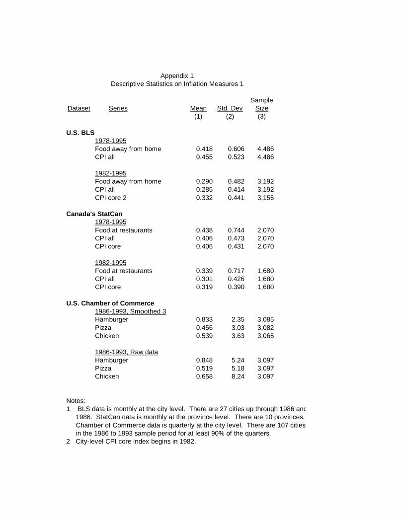
Appendix 1 reports descriptive statistics on the key price variables for each data set. Not

surprisingly, restaurant inflation is more variable than broader CPI measures. The smoothed

ACCRA data have roughly the same variance as the BLS and StatCan restaurant inflation

variables after accounting for the difference in frequency in the data. However, the standard

deviation of the raw ACCRA data are approximately twice as high as the smoothed data. The

chicken data are especially noisy relative to the other food products, but the standard deviation is

reduced from 8.24 to 3.63 by the smoothing techniques.

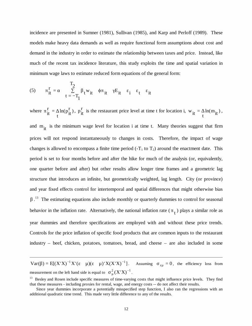
IV. Empirical Strategy and Results

The empirical strategy is to relate price changes in the restaurant industry at time t in

location i to changes in the minimum wage. Attempts to estimate structural models of tax

12 Suppose the measured dependent variable ( πit ) is the sum of the true value ( πit

* ) and measurement error

(µ it ). The variance matrix of the OLS estimator is then

12

incidence are presented in Sumner (1981), Sullivan (1985), and Karp and Perloff (1989). These

models make heavy data demands as well as require functional form assumptions about cost and

demand in the industry in order to estimate the relationship between taxes and price. Instead, like

much of the recent tax incidence literature, this study exploits the time and spatial variation in

minimum wage laws to estimate reduced form equations of the general form:

(5) π α β ϕπ γ ε ε εitr

twitt T

T

it Eit i t it= += −∑ + + + + +

1

2

where πitr

tpit

r= ∆ ln( ) , pitr is the restaurant price level at time t for location i, wit t

mit= ∆ ln( ) ,

and mit is the minimum wage level for location i at time t. Many theories suggest that firm

prices will not respond instantaneously to changes in costs. Therefore, the impact of wage

changes is allowed to encompass a finite time period (-T1 to T2) around the enactment date. This

period is set to four months before and after the hike for much of the analysis (or, equivalently,

one quarter before and after) but other results allow longer time frames and a geometric lag

structure that introduces an infinite, but geometrically weighted, lag length. City (or province)

and year fixed effects control for intertemporal and spatial differences that might otherwise bias

β .13 The estimating equations also include monthly or quarterly dummies to control for seasonal

behavior in the inflation rate. Alternatively, the national inflation rate ( πt ) plays a similar role as

year dummies and therefore specifications are employed with and without these price trends.

Controls for the price inflation of specific food products that are common inputs to the restaurant

industry – beef, chicken, potatoes, tomatoes, bread, and cheese – are also included in some

Var E X X X X X X( ) [( ) ( )( ) ( ) ]β ε µ ε µ= ′ ′ + + ′ ′− −1 1 . Assuming σεµ = 0 , the efficiency loss from

measurement on the left hand side is equal to σµ2 1( )′ −X X .

13 Besley and Rosen include specific measures of time-varying costs that might influence price levels. They findthat these measures - including proxies for rental, wage, and energy costs -- do not affect their results. Since year dummies incorporate a potentially misspecified step function, I also ran the regressions with anadditional quadratic time trend. This made very little difference to any of the results.

13

specifications. BLS and StatCan national food prices are used because these products are

typically sold in national markets. Finally, I also include overall city or province-specific inflation

( πit ) and state employment conditions ( Eit ) to control for local inflation trends. However, local

price trends may be affected by the minimum wage increase and therefore could lead to an

understatement of β .

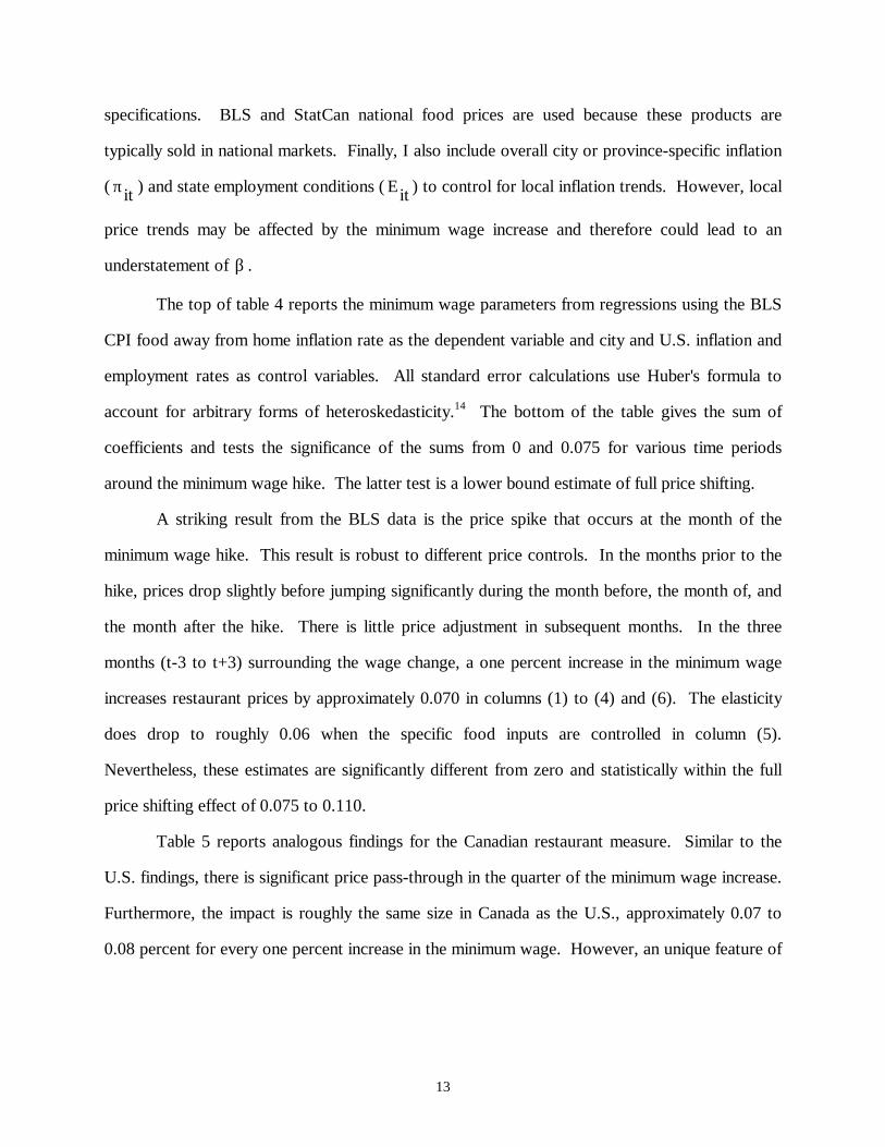
The top of table 4 reports the minimum wage parameters from regressions using the BLS

CPI food away from home inflation rate as the dependent variable and city and U.S. inflation and

employment rates as control variables. All standard error calculations use Huber's formula to

account for arbitrary forms of heteroskedasticity.14 The bottom of the table gives the sum of

coefficients and tests the significance of the sums from 0 and 0.075 for various time periods

around the minimum wage hike. The latter test is a lower bound estimate of full price shifting.

A striking result from the BLS data is the price spike that occurs at the month of the

minimum wage hike. This result is robust to different price controls. In the months prior to the

hike, prices drop slightly before jumping significantly during the month before, the month of, and

the month after the hike. There is little price adjustment in subsequent months. In the three

months (t-3 to t+3) surrounding the wage change, a one percent increase in the minimum wage

increases restaurant prices by approximately 0.070 in columns (1) to (4) and (6). The elasticity

does drop to roughly 0.06 when the specific food inputs are controlled in column (5).

Nevertheless, these estimates are significantly different from zero and statistically within the full

price shifting effect of 0.075 to 0.110.

Table 5 reports analogous findings for the Canadian restaurant measure. Similar to the

U.S. findings, there is significant price pass-through in the quarter of the minimum wage increase.

Furthermore, the impact is roughly the same size in Canada as the U.S., approximately 0.07 to

0.08 percent for every one percent increase in the minimum wage. However, an unique feature of

14

the Canadian price response is the monthly pattern. The impact is very small leading up to and

including the month of the wage legislation's starting date. The price changes begin occurring the

month after the minimum wage change (t+l) and continue through the third month (t+3). The t+3

coefficient is roughly the same magnitude as the U.S. month t coefficient. Therefore, assuming

the fraction of minimum wage workers and the share of labor cost is the same in Canada as the

U.S., there appears to be evidence of full cost shifting in Canada.

Table 6 shows the results using the ACCRA price data. The data are reported quarterly

and therefore only a single lag and lead is included, but these three quarters encompass the same

amount of time as the four month lags and leads of the previous tables. Three sets of results are

reported for each of the three food products. Columns (1), (5), and (9) report the results when

using the raw data published in ACCRA's Cost of Living Index. Columns (2), (6), and (10) adjust

for the temporary and large time-series spikes by smoothing out any quarterly price change that

exceeds five percent and does not persist for at least three quarters. The final two columns for

each food item use the smoothed data but control for U.S. price trends in food at home and

overall inflation or the specific food products noted already. All regressions include month, year,

and city fixed effects.

For hamburgers, the raw data show roughly the same size sum of coefficients as the more

aggregated CPI restaurant measures. Furthermore, like the BLS data, nearly all of the inflation

response occurs within the quarter of the law's enactment. The pizza and chicken responses are

zero and, in some cases, negative. However, smoothing the data to eliminate the large spikes

results in much larger estimates of the impact of minimum wage changes on hamburger and fried

chicken prices. These regressions suggest a 0.12 to 0.16 percent increase in hamburger and

chicken prices for every one percent increase in the minimum wage.

14 To correct for possible autocorrelation in area-specific inflation rates, Newey-West standard errors are alsocomputed. However, the Huber and Newey-West standard errors are similar and therefore the latter are notreported.

15

There are a number of explanations for the different price responses found in the ACCRA

and BLS/StatCan data. First, these findings are consistent with the different price responses

found in the tax incidence studies of Poterba (1996), who finds full shifting using the BLS apparel

indices, and Besley and Rosen (1994), who find overshifting using the ACCRA clothing indices.15

Second, fast food restaurants, like McDonald's and Kentucky Fried Chicken, may have more

workers affected by a change in the minimum wage than restaurants in general. These

establishments tend to comply with minimum wage laws and do not allow tipping, so there is

likely to be a larger impact on prices. If 50 percent of workers at these fast food chains were

impacted by these wage laws, the 0.15 finding would be consistent with full pass-through.

Given the noisiness of the ACCRA data, another possibility is that the larger coefficients

are driven by outliers. Therefore, the regressions were rerun using a robustness technique that

weights observations based on an initial regression. Observations with large residuals are

assigned lower weights. Those with small residuals receive weights approaching one.16 The

results are reported in table 7. Regressions with city and year fixed effects show total elasticities

ranging from 0.035 for pizza to 0.073 for hamburgers. However, note that because of the

noisiness of this data, up to 500 observations receive weights of less than 0.1 in some regressions.

This is so even after the data have been smoothed to eliminate the extreme, temporary price

spikes. Nevertheless, the robustness regression results are in line with the findings using the more

aggregated BLS and StatCan data.

Curiously, the impact on pizza prices reported in table 6 is zero or negative even after

smoothing out the inexplicable spikes in the data. Part of this surprising finding is due to outliers,

as shown by the results in table 7. Further experimentation suggests that much of the

15 It is not clear why aggregation matters. Besley and Rosen argue that the BLS indices comprise a variety ofproducts that vary over time and across areas, making the results more difficult to interpret.16 The estimation technique calculates Huber weights and biweights (see Berk 1990 for a description). Huberweights are used as a starting value for the biweight iteration. Both weights are used because Huber has troubledealing with extreme outliers and biweights sometimes do not converge. Iterations stop when the maximumchange in weights drops below a tolerance level.

16

inconsequential pizza price response is driven by the April 1991 federal minimum wage increase.17

Table 8 decomposes the quarterly price changes by whether there is a minimum wage hike.

Columns (1) and (2) show the mean price change for 1991 and columns (3) and (4) for 1986 to

1990 and 1992 to 1993. In 1991, pizza and chicken inflation were lower in the quarters without a

minimum wage hike, whereas the remaining years show the expected pattern of higher price

growth in quarters with such labor cost changes. If this 1991 federal increase is excluded from

the sample, the three quarter sum of coefficients for pizza is 0.084, still below the hamburger and

chicken price effects, but roughly in line with the full pass-through prediction. The chicken price

coefficients rise slightly as well when 1991 data are excluded. Alternatively, if I rerun the pizza

regressions with separate federal and state minimum wage change variables, the total elasticity is

-0.134 for the federal increases and 0.148 for the state increases. The state pizza elasticity is

roughly the same magnitude as the chicken and hamburger findings. The state-federal

classification has no effect on the hamburger or chicken elasticities or on the BLS food away from

home elasticity.

It is difficult to know why the 1991 price response was different, especially for pizza and

chicken restaurants. However, it appears to be a recurring finding. Katz and Krueger's (1992)

independent survey of Kentucky Fried Chicken, Burger King, and Wendy’s restaurants in Texas

also found little price pass-through due to the April 1991 federal minimum wage increase. The

bottom of table 8 confirms Katz and Krueger’s finding of small, and even negative, price

responses in 1991 among hamburger and chicken (but not pizza) restaurants in nine Texas cities

using the ACCRA data.18 Furthermore, smaller April 1991 price effects also occur in the BLS

17 Another explanation for the smaller Pizza Hut findings is that their production plan is different: labor share orthe fraction of workers affected by minimum wage legislation is lower and, correspondingly, price responses arelessened. Labor share appears to be the same; American Restaurant Partners, one of the restaurants in my SECsample and owners of 60 Pizza Huts throughout the U.S., has labor share of 29 percent in 1995 (compared to 30percent for the entire restaurant sample). However, it is plausible that the fraction of low wage workers isdifferent. Many Pizza Huts are sit down establishments where some employees are tipped.18 Two of the 11 Texas cities in the sample are missing data for the second quarter of 1991.

17

data. The price elasticity using the 1982 to 1995 time period is approximately 0.048, but the

elasticity rises to 0.064 if 1991 data is removed.

Several other robustness checks are made of the ACCRA results. First, since there are

multiple cities in each state, I averaged data across states and reran the equations using state-level

prices. This can be thought of as another smoothing filter on the data. The results are very

similar to those reported in table 6. When the sample is restricted to those states in the sample 90

percent of the quarters, the three quarter sum of coefficients are 0.152, -0.062, and 0.134 for

hamburgers, pizza, and chicken. Using only those states that appear in all 32 quarters does not

change any inferences; the sums are 0.169, 0.001, and 0.112.

Second, I deleted cities that are on the borders of other states. Border cities could be a

problem since they are under the influence of legislation from multiple states. As a result, demand

elasticities may be different for border and nonborder cities if consumers can cross borders to

purchase products. Furthermore, some restaurants may be influenced by the new legislation to

raise prices, while others are not affected by the law and are geographically sufficiently separated

enough from those that are that they do not to have to raise prices. This situation could

mechanically lower price estimates even when full shifting is occurring. In the 107 city sample,

there are 20 border cities but only 12 that have differences in minimum wage levels at any time

between 1986 and 1993. When the equations are rerun without these 12 cities, the impact on the

results is minimal. There is a slight increase in the hamburger results but the pizza and chicken

findings are essentially the same.

Longer Run Estimates

Baker et al (1995) show that the difference between short and long run responses can

reconcile different findings on minimum wage employment effects. Likewise, four months might

not be enough time to capture the entire price response to the new law. Therefore, table 9

displays two alternative specifications: an unconstrained lag structure that extends the lag and lead

time around the enactment month to nine months (i.e. T1 and T2 in equation (5) are set to 9) and

18

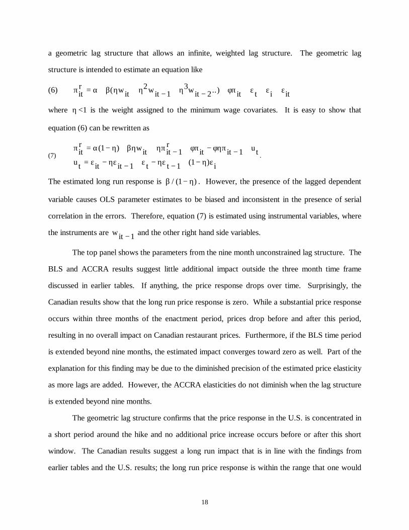
a geometric lag structure that allows an infinite, weighted lag structure. The geometric lag

structure is intended to estimate an equation like

(6) π α β η η η φπ ε ε εitr wit wit wit it t i it= + + − + − + + + +( ..)2

13

2

where η <1 is the weight assigned to the minimum wage covariates. It is easy to show that

equation (6) can be rewritten as

(7)π α η βη ηπ φπ φηπ

ε ηε ε ηε η εitr wit it

rit it ut

ut it it t t i

= − + + − + − − += − − + − − + −

( )

( )

1 1 1

1 1 1.

The estimated long run response is β η/ ( )1 − . However, the presence of the lagged dependent

variable causes OLS parameter estimates to be biased and inconsistent in the presence of serial

correlation in the errors. Therefore, equation (7) is estimated using instrumental variables, where

the instruments are wit − 1 and the other right hand side variables.

The top panel shows the parameters from the nine month unconstrained lag structure. The

BLS and ACCRA results suggest little additional impact outside the three month time frame

discussed in earlier tables. If anything, the price response drops over time. Surprisingly, the

Canadian results show that the long run price response is zero. While a substantial price response

occurs within three months of the enactment period, prices drop before and after this period,

resulting in no overall impact on Canadian restaurant prices. Furthermore, if the BLS time period

is extended beyond nine months, the estimated impact converges toward zero as well. Part of the

explanation for this finding may be due to the diminished precision of the estimated price elasticity

as more lags are added. However, the ACCRA elasticities do not diminish when the lag structure

is extended beyond nine months.

The geometric lag structure confirms that the price response in the U.S. is concentrated in

a short period around the hike and no additional price increase occurs before or after this short

window. The Canadian results suggest a long run impact that is in line with the findings from

earlier tables and the U.S. results; the long run price response is within the range that one would

19

expect to see in full pass-through situations. However, these parameters are not well estimated.

Only the BLS coefficients are statistically different from zero. If OLS is used instead of IV, the

BLS and StatCan long run coefficients are approximately 0.03 and are statistically different from

0 and 0.075, suggesting partial pass-through in the long run. The ACCRA hamburger, chicken,

and pizza coefficients are 0.060, 0.074, and -0.006, respectively. The former two are different

from zero and the latter is different from 0.075 at the five percent level. Therefore, the evidence

in table 9 is mixed. The unconstrained and some of the geometric U.S. and Canadian CPI results

suggest that price shifting dissipates over time; other findings, especially using the ACCRA data,

confirm full or close to full price pass-through predictions.

Effects on Broader Price Measures

Table 10 reports the minimum wage coefficients from a regression using the BLS's and

StatCan's CPI core and CPI for all products. As explained in section II, the predicted elasticity

for broader CPI measures is approximately 0.015 to 0.020. Column (1) displays the overall BLS

CPI regressions using data from 1978 to 1995. Surprisingly, the impact is about 0.04, suggesting

substantial overshifting of prices. This finding may be driven by the January 1979 federal

minimum wage increase, which coincided with the beginning of the OPEC oil shock. However,

controlling for energy inflation makes little difference. Alternatively, I reran the regressions but

started the data in 1982, well after reverberations from the oil shock and the resulting recession.

This time period is also useful because city-specific core CPI prices began to be computed in

1982. Columns (2) and (3) show that this shorter period suggests smaller minimum wage

elasticities. When controlling for energy inflation, the minimum wage price pass-through is

approximately 0.012, not statistically different from the predicted full shifting effect. Using the

core CPI rate, negative price responses are found. These results are similar when looking at

longer run responses using unconstrained or geometric lag structures. The difference in the

1978-1995 and 1982-1995 findings is consistent with the assertion in Cecchetti (1986) that firms

are more able to adjust prices during periods of high inflation.

20

The Canadian results are similar to the BLS results in some important respects. When

exploring a time frame that begins in the late 1970s (columns 4 and 6), the impact on the core and

overall CPI is roughly 0.010, in line with the expected impact, although much smaller than the

U.S. elasticity. When the volatile early years are excluded (columns 5 and 7), the effect drops and

is even negative for the overall CPI. The magnitude of these latter findings is consistent with the

U.S. CPI results. However, because of the much smaller predicted effect of 0.015 to 0.02 and the

size of the standard errors, it is difficult to statistically differentiate a zero and full shifting effect in

the U.S. or Canadian parameters. The most that can be said about these results is that some cost

shifting may take place in the overall economy, but these effects are not nearly as large as they

once were in the late 1970s and early 1980s (this is also true of the restaurant sample) and

statistically cannot be distinguished from a zero pass-through scenario.19

Is Minimum Wage Legislation Endogenous?

It is plausible that state and federal legislators may become more concerned with the

deteriorating real value of minimum wages during periods of high inflation. As a result, the

estimated minimum wage elasticity may be biased upward; persistently high inflation rates may

cause an increase in the minimum wage rather than the other way around. However, this pattern

is also consistent with the evidence on firm behavior presented in Cecchetti (1986) and therefore

is not prima facie evidence of an endogeneity problem. Furthermore, time and city fixed effects

should account for unusually high inflation periods. Nevertheless, I tested for the possibility of an

endogeneity problem by looking at inflation patterns before the enactment of minimum wage

legislation (i.e. when legislation is debated and passed). Fortunately, in the BLS and StatCan

19 Because of the imprecision of the parameters, it is dangerous to make too much of the small pass-through foundfor the broader CPI measures. However, there are reasons to think that pass-through would be partial in thesecases. First, restaurants tend to be local; therefore, every firm faces a similar cost structure. In national markets,firms must compete with others who do not experience an increase in minimum wages, and therefore it may bemore difficult to pass-through minimum wage hikes. Second, there is little shifting of production in the restaurantindustry due to minimum wage changes. For example, Card and Krueger (1995) find no minimum wage impacton McDonald's openings or closings. However, Gron and Swenson (1996) find that this is a strategy employed byinternational firms to avoid price increases resulting from exchange rate fluctuations. National firms that are hithard by minimum wage changes may employ this production shifting strategy as well.

21

data, there is virtually no evidence that inflation is higher in the two years prior to the legislation’s

enactment date. The possible exception to this finding is when U.S. state increases are analyzed

separately. The endogeneity problem may be more severe in the case of state legislation.

However, reestimating the BLS and ACCRA regressions with separate federal and state minimum

wage covariates shows no difference in the state or federal coefficients except among the ACCRA

pizza parameters. Therefore, I conclude that there is little reason to be concerned about

endogeneity in this analysis.

V. Conclusions

Using a variety of data sources on restaurant prices, this paper tests a textbook

consequence of competitive markets: an industry-wide increase in the price of inputs will be

passed on to consumers through an increase in prices. Estimates of price shifting can have

important implications for wage-push inflation stories, as well as potentially provide an

explanation for the small short-run employment effects that have been found in some of the

minimum wage literature. The results suggest that restaurant prices rise roughly one-for-one with

increases in the wage bill that result from minimum wage legislation. Furthermore, the price

responses are concentrated in the quarter surrounding the month that the legislation is enacted.

Although minimum wage legislation is typically enacted many months in advance, there is no price

response leading up to the hike and little adjustment in the months subsequent to the hike,

excepting the few months around the enactment date. If anything, there is some evidence that

minimum wage price effects dissipate over time. The magnitude of these findings is roughly the

same in the U.S. and Canada, and is fairly robust to changes in data, specification, and estimation

techniques. However, because of small predicted elasticities, it is difficult to draw inferences

about the price impact on broader indices or industries that have a small share of low wage labor.

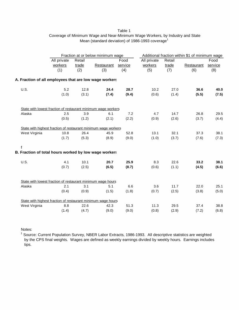
Table 1Coverage of Minimum Wage and Near-Minimum Wage Workers, by Industry and State

Mean (standard deviation) of 1986-1993 coverage 1

Fraction at or below minimum wage Additional fraction within $1 of minimum wageAll private Retail Food All private Retail Food workers trade Restaurant service workers trade Restaurant service

(1) (2) (3) (4) (5) (7) (6) (8)

A. Fraction of all employees that are low wage workers

U.S. 5.2 12.8 24.4 28.7 10.2 27.0 36.6 40.0(1.0) (3.1) (7.4) (9.4) (0.6) (1.4) (5.5) (7.5)

State with lowest fraction of restaurant minimum wage workersAlaska 2.5 3.9 6.1 7.2 4.7 14.7 26.8 29.5

(0.5) (1.2) (2.1) (2.2) (0.9) (2.6) (3.7) (4.4)

State with highest fraction of restaurant minimum wage workersWest Virginia 10.8 26.4 45.9 52.8 13.1 32.1 37.3 38.1

(1.7) (5.3) (8.9) (9.0) (1.0) (3.7) (7.6) (7.3)

fB. Fraction of total hours worked by low wage workers

U.S. 4.1 10.1 20.7 25.9 8.3 22.6 33.2 38.1(0.7) (2.5) (6.5) (8.7) (0.6) (1.1) (4.5) (6.6)

State with lowest fraction of restaurant minimum wage hoursAlaska 2.1 3.1 5.1 6.6 3.6 11.7 22.0 25.1

(0.4) (0.9) (1.5) (1.8) (0.7) (2.5) (3.8) (5.0)

State with highest fraction of restaurant minimum wage hoursWest Virginia 8.8 22.6 42.3 51.3 11.3 29.5 37.4 38.8

(1.4) (4.7) (9.0) (9.0) (0.8) (2.9) (7.2) (6.8)

Notes:1 Source: Current Population Survey, NBER Labor Extracts, 1986-1993. All descriptive statistics are weighted by the CPS final weights. Wages are defined as weekly earnings divided by weekly hours. Earnings includes tips.

Table 2U.S. Minimum Wage Increases, by State and Year, 1978-1995 1

Not including

changes within 6 monthsAll of a federal increase

Average AverageNumber of percent Number of percentincreases increase increases increase

(1) (2) (3) (4)

U.S. increases 6 4.4

By StateAlaska 2 7 3.9 0California 1 10.3 1 10.3Connecticut 2 5.0 2 5.0Hawaii 3 5.1 3 5.1Iowa 3 4.7 1 3.9Maine 5 1.2 4 1.2Massachusetts 3 1.6 3 1.6Minnesota 4 2.6 3 2.4New Hampshire 5 1.1 3 1.2New Jersey 1 7.5 1 7.5Oregon 3 5.1 3 5.1Pennsylvania 1 4.3 1 4.3Rhode Island 5 2.5 5 2.5Vermont 6 1.4 5 1.6Washington 3 5.5 3 5.5Wisconsin 1 3.7 1 3.7

Total 53 #REF! 39 0.0

State Increases, By Year 3

1978-1984 4 0 01985 1 1.3 1 1.31986 4 1.9 4 1.91987 6 1.8 6 1.81988 8 4.0 8 4.01989 9 3.3 9 3.31990 4 7 2.7 3 3.21991 4 5 3.0 2 3.41992 3 5.4 3 5.41993 1 4.3 1 4.31994 1 6.2 1 6.21995 1 2.5 1 2.5

Notes:1 Does not include Washington D.C. The state minimum wage is taken as the maximum of the federal and state level.2 Alaska law requires the state minimum wage be $0.50 above the federal level.3 Not including Alaska or federal increases.4 Year with federal minimum wage hike. Annual federal increases occurred between 1978 and 1981.

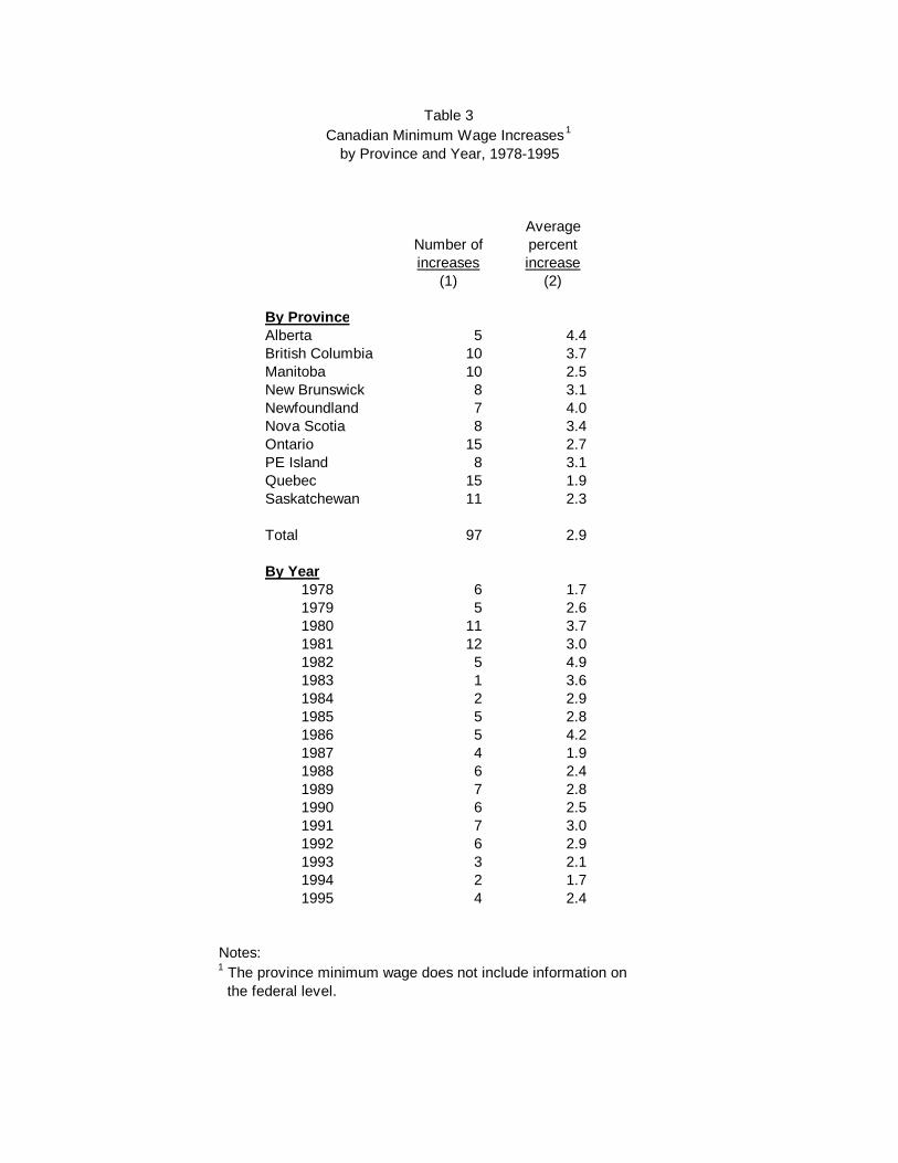
Table 3Canadian Minimum Wage Increases 1

by Province and Year, 1978-1995

AverageNumber of percentincreases increase

(1) (2)

By ProvinceAlberta 5 4.4British Columbia 10 3.7Manitoba 10 2.5New Brunswick 8 3.1Newfoundland 7 4.0Nova Scotia 8 3.4Ontario 15 2.7PE Island 8 3.1Quebec 15 1.9Saskatchewan 11 2.3

Total 97 2.9

By Year1978 6 1.71979 5 2.61980 11 3.71981 12 3.01982 5 4.91983 1 3.61984 2 2.91985 5 2.81986 5 4.21987 4 1.91988 6 2.41989 7 2.81990 6 2.51991 7 3.01992 6 2.91993 3 2.11994 2 1.71995 4 2.4

Notes:1 The province minimum wage does not include information on the federal level.

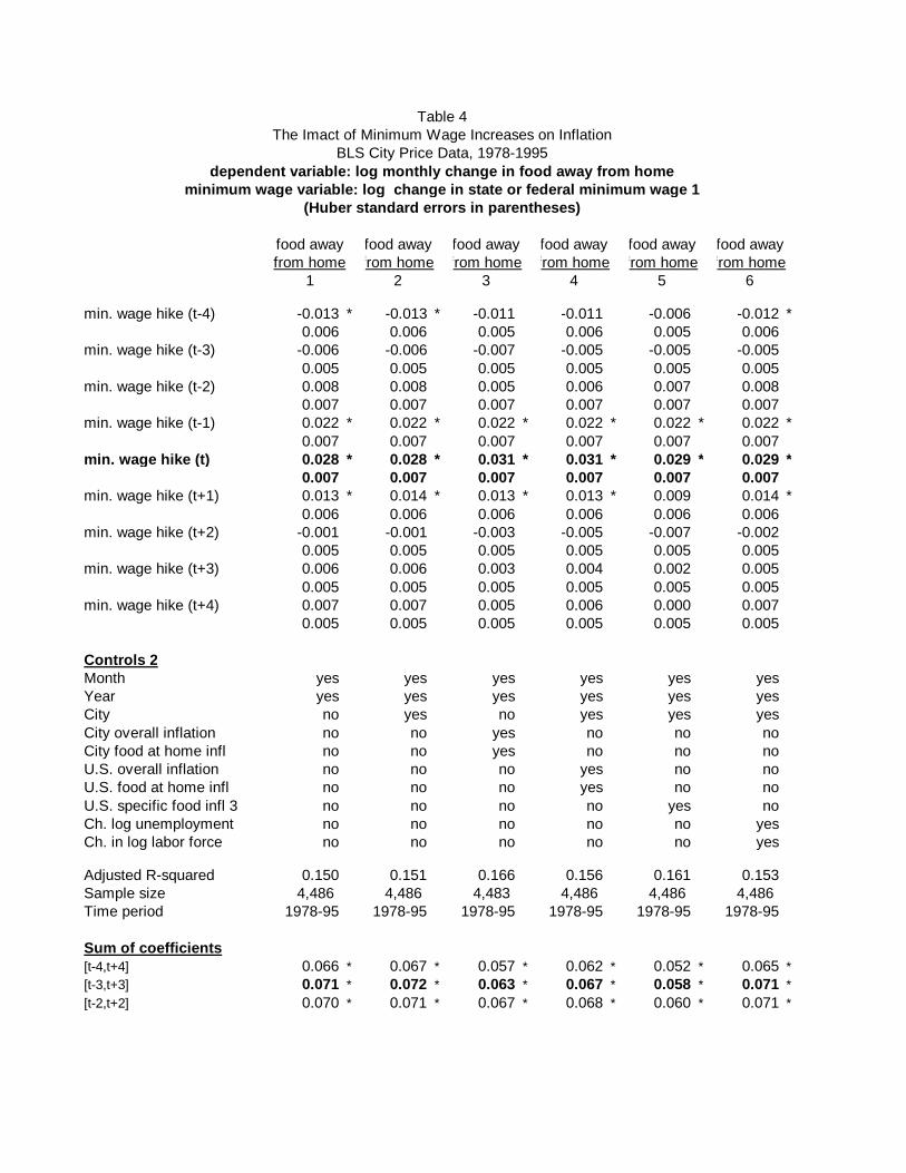
Table 4The Imact of Minimum Wage Increases on Inflation

BLS City Price Data, 1978-1995dependent variable: log monthly change in food away from home

minimum wage variable: log change in state or federal minimum wage 1(Huber standard errors in parentheses)

food awayfood awayfood awayfood awayfood awayfood awayfrom homefrom homefrom homefrom homefrom homefrom home

654321

*-0.012-0.006-0.011-0.011*-0.013*-0.013min. wage hike (t-4)0.0060.0050.0060.0050.0060.006

-0.005-0.005-0.005-0.007-0.006-0.006min. wage hike (t-3)0.0050.0050.0050.0050.0050.0050.0080.0070.0060.0050.0080.008min. wage hike (t-2)0.0070.0070.0070.0070.0070.007

*0.022*0.022*0.022*0.022*0.022*0.022min. wage hike (t-1)0.0070.0070.0070.0070.0070.007

*0.029*0.029*0.031*0.031*0.028*0.028min. wage hike (t)0.0070.0070.0070.0070.0070.007

*0.0140.009*0.013*0.013*0.014*0.013min. wage hike (t+1)0.0060.0060.0060.0060.0060.006

-0.002-0.007-0.005-0.003-0.001-0.001min. wage hike (t+2)0.0050.0050.0050.0050.0050.0050.0050.0020.0040.0030.0060.006min. wage hike (t+3)0.0050.0050.0050.0050.0050.0050.0070.0000.0060.0050.0070.007min. wage hike (t+4)0.0050.0050.0050.0050.0050.005

Controls 2yesyesyesyesyesyesMonth yesyesyesyesyesyesYearyesyesyesnoyesnoCitynononoyesnonoCity overall inflationnononoyesnonoCity food at home inflnonoyesnononoU.S. overall inflationnonoyesnononoU.S. food at home inflnoyesnonononoU.S. specific food infl 3

yesnononononoCh. log unemploymentyesnononononoCh. in log labor force

0.1530.1610.1560.1660.1510.150Adjusted R-squared4,4864,4864,4864,4834,4864,486Sample size

1978-951978-951978-951978-951978-951978-95Time period

Sum of coefficients*0.065*0.052*0.062*0.057*0.067*0.066[t-4,t+4]*0.071*0.058*0.067*0.063*0.072*0.071[t-3,t+3]*0.071*0.060*0.068*0.067*0.071*0.070[t-2,t+2]

*0.053*0.054*0.054*0.050*0.053*0.052[t-3,t]*#0.047*#0.034*#0.044*#0.043*#0.047*#0.047[t,t+3]

Notes:1 *=significantly different from 0 at the 5 percent level. #=sum of coefficients are significantly different from 0.075 at the 5 percent level.2 Price and unemployment controls include current and lagged monthly variables.3 Specific U.S. food inflation include BLS city averages for beef, chicken, bread, potatoes, cheese, and tomatoes.

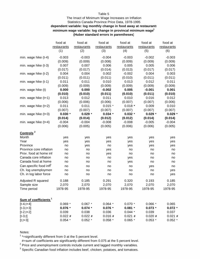
Table 5The Imact of Minimum Wage Increases on InflationStatistics Canada Province Price Data, 1978-1995

dependent variable: log monthly change in food away at restaurantsminimum wage variable: log change in provincal minimum wage 1

(Huber standard errors in parentheses)

food at food at food at food at food at food atrestaurants restaurants restaurants restaurants restaurants restaurants

(1) (2) (3) (4) (5) (6)

min. wage hike (t-4) -0.003 -0.003 -0.004 -0.003 -0.002 -0.003(0.009) (0.009) (0.008) (0.009) (0.009) (0.009)

min. wage hike (t-3) 0.007 0.007 0.006 0.005 0.005 0.006(0.017) (0.017) (0.014) (0.013) (0.017) (0.017)

min. wage hike (t-2) 0.004 0.004 0.002 -0.002 0.004 0.003(0.011) (0.011) (0.011) (0.010) (0.011) (0.011)

min. wage hike (t-1) 0.011 0.011 0.010 0.013 0.012 0.011(0.009) (0.009) (0.009) (0.009) (0.009) (0.009)

min. wage hike (t) 0.000 0.000 -0.002 0.005 -0.001 0.001(0.010) (0.010) (0.011) (0.010) (0.011) (0.010)

min. wage hike (t+1) 0.013 0.012 0.011 0.010 0.016 0.012(0.006) (0.006) (0.006) (0.007) (0.007) (0.006)

min. wage hike (t+2) 0.011 0.011 0.015 * 0.018 * 0.009 0.010(0.007) (0.007) (0.007) (0.007) (0.007) (0.007)

min. wage hike (t+3) 0.030 * 0.029 * 0.034 * 0.032 * 0.029 * 0.029 *(0.014) (0.014) (0.012) (0.012) (0.014) (0.014)

min. wage hike (t+4) -0.004 -0.004 -0.008 -0.008 -0.005 -0.004(0.006) (0.005) (0.005) (0.006) (0.006) (0.005)

Controls 2

Month yes yes yes yes yes yesYear yes yes yes yes yes yesProvince no yes no yes yes yesProvince core inflation no no yes no no noProv. food at home infl no no yes no no noCanada core inflation no no no yes no noCanada food at home infl no no no yes no noCan.specific food infl3 no no no no yes noCh. log unemployment no no no no no yesCh. in log labor force no no no no no yes

Adjusted R squared 0.188 0.185 0.291 0.320 0.193 0.185Sample size 2,070 2,070 2,070 2,070 2,070 2,070Time period 1978-95 1978-95 1978-95 1978-95 1978-95 1978-95

Sum of coefficients 1

[t-4,t+4] 0.069 * 0.067 * 0.064 * 0.070 * 0.066 * 0.065[t-3,t+3] 0.076 * 0.074 * 0.076 * 0.081 * 0.073 * 0.072 *[t-2,t+2] 0.039 0.038 0.036 0.044 * 0.039 0.037[t-3,t] 0.022 # 0.022 # 0.016 # 0.021 # 0.020 # 0.021 #[t,t+3] 0.054 * 0.052 * 0.058 * 0.065 * 0.053 * 0.052 *

Notes:1 *=significantly different from 0 at the 5 percent level. #=sum of coefficients are significantly different from 0.075 at the 5 percent level.2 Price and unemployment controls include current and lagged monthly variables.3 Specific Canadian food inflation includes beef, chicken, potatoes, and tomatoes.

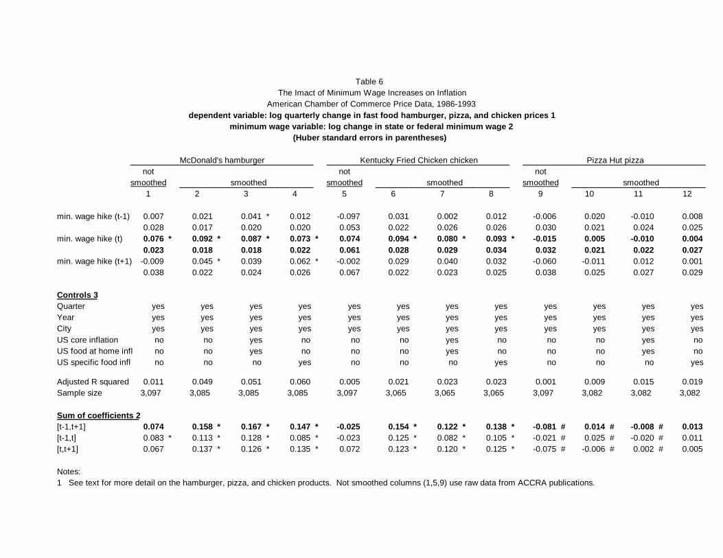
Table 6The Imact of Minimum Wage Increases on Inflation

American Chamber of Commerce Price Data, 1986-1993dependent variable: log quarterly change in fast food hamburger, pizza, and chicken prices 1

minimum wage variable: log change in state or federal minimum wage 2(Huber standard errors in parentheses)

Pizza Hut pizzaKentucky Fried Chicken chickenMcDonald's hamburgernotnotnot

smoothedsmoothedsmoothedsmoothedsmoothedsmoothed121110987654321

0.008-0.0100.020-0.0060.0120.0020.031-0.0970.012*0.0410.0210.007min. wage hike (t-1)0.0250.0240.0210.0300.0260.0260.0220.0530.0200.0200.0170.0280.004-0.0100.005-0.015*0.093*0.080*0.0940.074*0.073*0.087*0.092*0.076min. wage hike (t)0.0270.0220.0210.0320.0340.0290.0280.0610.0220.0180.0180.0230.0010.012-0.011-0.0600.0320.0400.029-0.002*0.0620.039*0.045-0.009min. wage hike (t+1)0.0290.0270.0250.0380.0250.0230.0220.0670.0260.0240.0220.038

Controls 3yesyesyesyesyesyesyesyesyesyesyesyesQuarteryesyesyesyesyesyesyesyesyesyesyesyesYearyesyesyesyesyesyesyesyesyesyesyesyesCitynoyesnononoyesnononoyesnonoUS core inflationnoyesnononoyesnononoyesnonoUS food at home infl

yesnononoyesnononoyesnononoUS specific food infl4

0.0190.0150.0090.0010.0230.0230.0210.0050.0600.0510.0490.011Adjusted R squared3,0823,0823,0823,0973,0653,0653,0653,0973,0853,0853,0853,097Sample size

Sum of coefficients 20.013#-0.008#0.014#-0.081*0.138*0.122*0.154-0.025*0.147*0.167*0.1580.074[t-1,t+1]0.011#-0.020#0.025#-0.021*0.105*0.082*0.125-0.023*0.085*0.128*0.113*0.083[t-1,t]0.005#0.002#-0.006#-0.075*0.125*0.120*0.1230.072*0.135*0.126*0.1370.067[t,t+1]

Notes:1 See text for more detail on the hamburger, pizza, and chicken products. Not smoothed columns (1,5,9) use raw data from ACCRA publications.

The data used in the smoothed columns eliminates temporary (less than 2 quarters) and large (> 5% quarterly change) spikes in the price data through linear interpolation. Sample sizes vary because spikes that occur in the first two and last two quarters of the sample are thrown out.2 *=significantly different from 0 at the 5 percent level. #=sum of coefficients are significantly different from 0.075 at the 5 percent level.3 Price controls include current and lagged quarterly variables.4 Specific U.S. food inflation include BLS city averages for beef, chicken, bread, potatoes, cheese, and tomatoes.

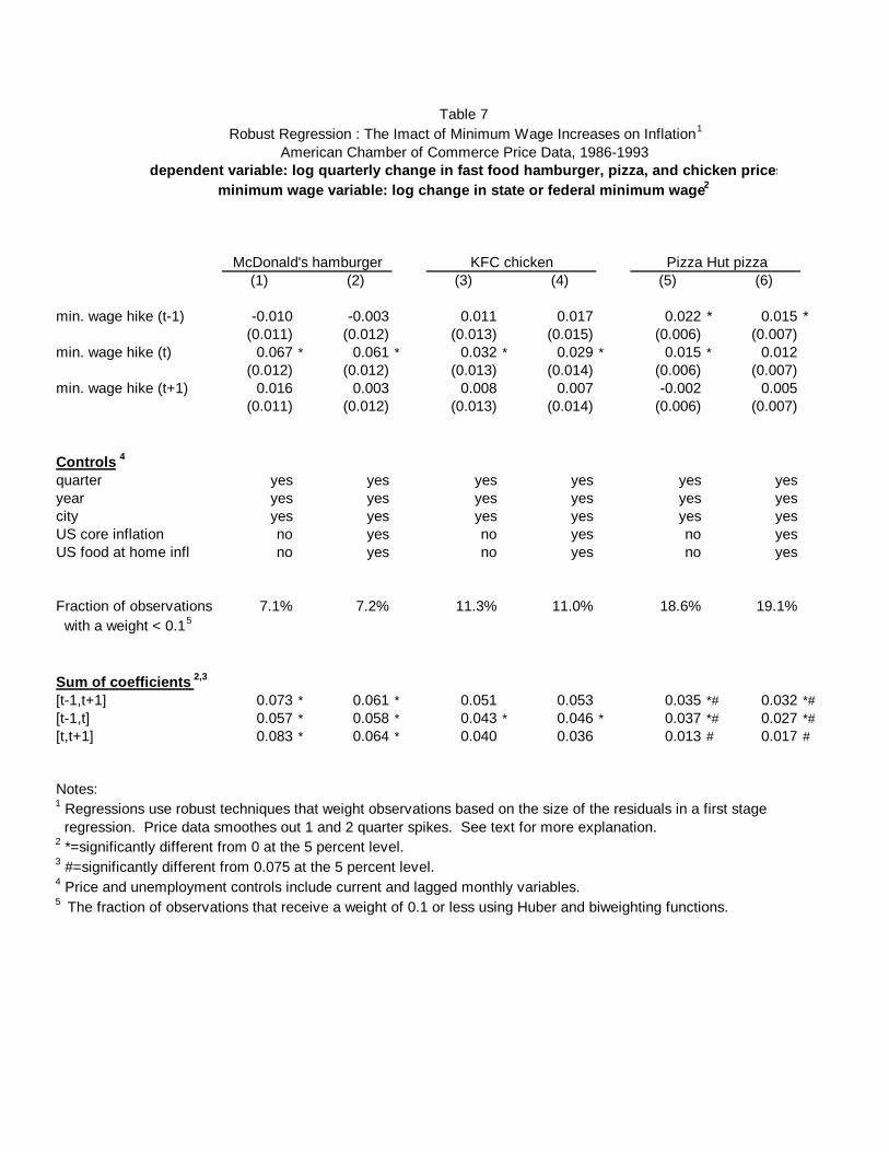
Table 7 Robust Regression : The Imact of Minimum Wage Increases on Inflation 1

American Chamber of Commerce Price Data, 1986-1993dependent variable: log quarterly change in fast food hamburger, pizza, and chicken prices

minimum wage variable: log change in state or federal minimum wage 2

McDonald's hamburger KFC chicken Pizza Hut pizza(1) (2) (3) (4) (5) (6)

min. wage hike (t-1) -0.010 -0.003 0.011 0.017 0.022 * 0.015 *(0.011) (0.012) (0.013) (0.015) (0.006) (0.007)

min. wage hike (t) 0.067 * 0.061 * 0.032 * 0.029 * 0.015 * 0.012(0.012) (0.012) (0.013) (0.014) (0.006) (0.007)

min. wage hike (t+1) 0.016 0.003 0.008 0.007 -0.002 0.005(0.011) (0.012) (0.013) (0.014) (0.006) (0.007)

Controls 4

quarter yes yes yes yes yes yesyear yes yes yes yes yes yescity yes yes yes yes yes yesUS core inflation no yes no yes no yesUS food at home infl no yes no yes no yes

Fraction of observations 7.1% 7.2% 11.3% 11.0% 18.6% 19.1% with a weight < 0.1 5

Sum of coefficients 2,3

[t-1,t+1] 0.073 * 0.061 * 0.051 0.053 0.035 *# 0.032 *#[t-1,t] 0.057 * 0.058 * 0.043 * 0.046 * 0.037 *# 0.027 *#[t,t+1] 0.083 * 0.064 * 0.040 0.036 0.013 # 0.017 #

Notes:1 Regressions use robust techniques that weight observations based on the size of the residuals in a first stage regression. Price data smoothes out 1 and 2 quarter spikes. See text for more explanation.2 *=significantly different from 0 at the 5 percent level.3 #=significantly different from 0.075 at the 5 percent level.4 Price and unemployment controls include current and lagged monthly variables.5 The fraction of observations that receive a weight of 0.1 or less using Huber and biweighting functions.

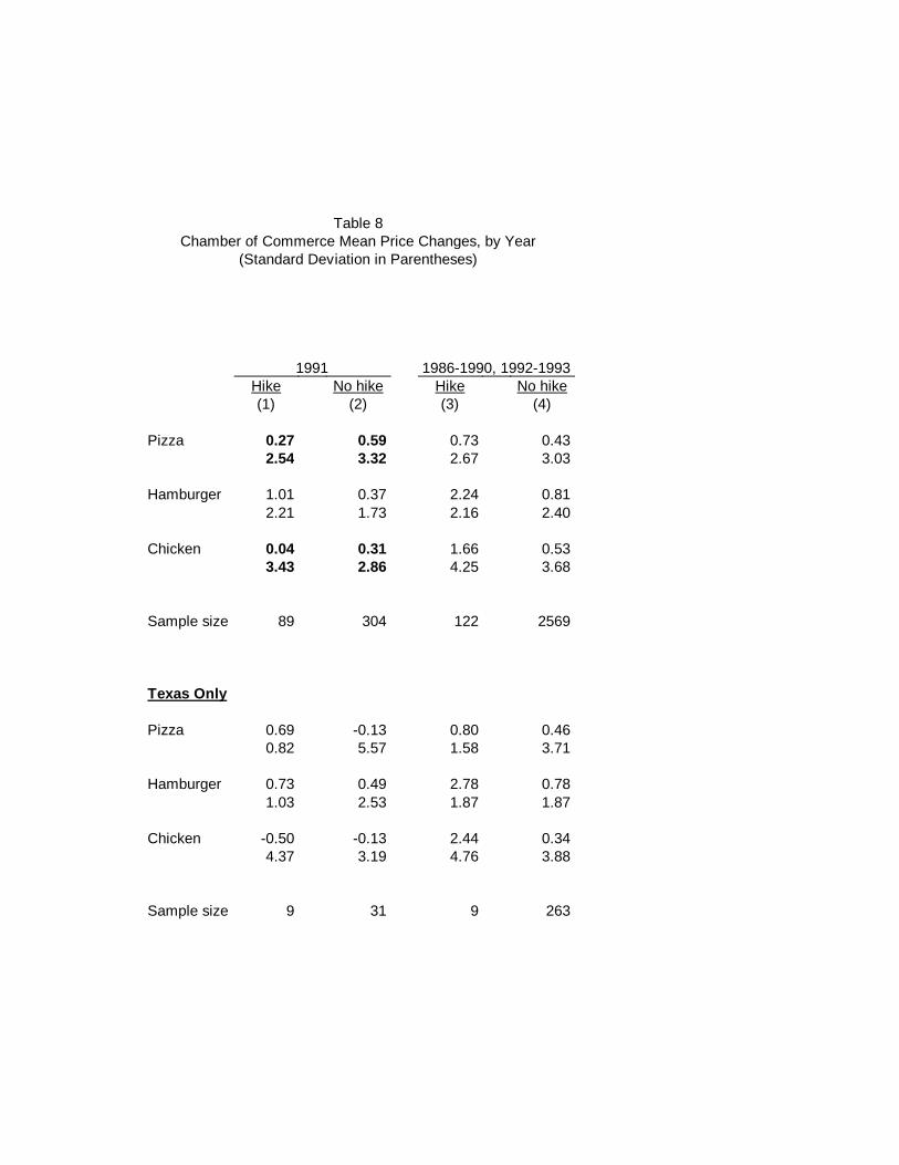
Table 8Chamber of Commerce Mean Price Changes, by Year

(Standard Deviation in Parentheses)

1986-1990, 1992-19931991No hikeHikeNo hikeHike

(4)(3)(2)(1)

0.430.730.590.27Pizza3.032.673.322.54

0.812.240.371.01Hamburger2.402.161.732.21

0.531.660.310.04Chicken3.684.252.863.43

256912230489Sample size

Texas Only

0.460.80-0.130.69Pizza3.711.585.570.82

0.782.780.490.73Hamburger1.871.872.531.03

0.342.44-0.13-0.50Chicken3.884.763.194.37

2639319Sample size

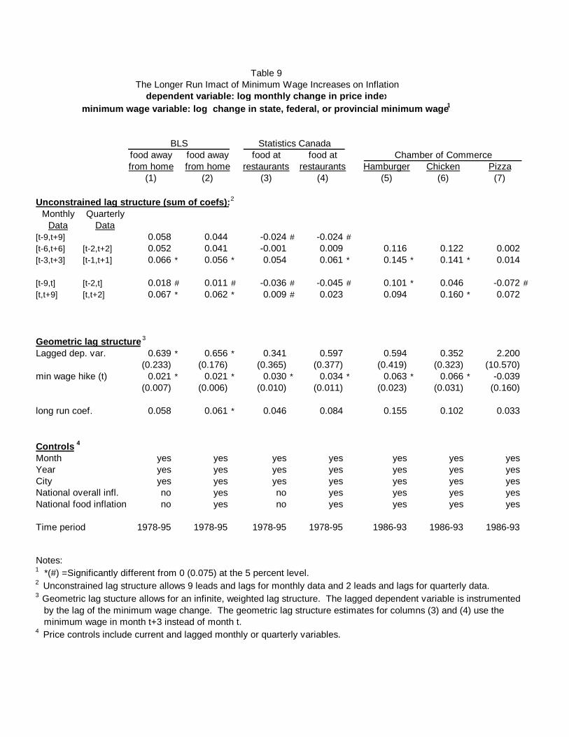
Table 9The Longer Run Imact of Minimum Wage Increases on Inflation

dependent variable: log monthly change in price indexminimum wage variable: log change in state, federal, or provincial minimum wage 1

BLS Statistics Canadafood away food away food at food at Chamber of Commercefrom home from home restaurants restaurants Hamburger Chicken Pizza

(1) (2) (3) (4) (5) (6) (7)

Unconstrained lag structure (sum of coefs): 2

Monthly QuarterlyData Data

[t-9,t+9] 0.058 0.044 -0.024 # -0.024 #[t-6,t+6] [t-2,t+2] 0.052 0.041 -0.001 0.009 0.116 0.122 0.002[t-3,t+3] [t-1,t+1] 0.066 * 0.056 * 0.054 0.061 * 0.145 * 0.141 * 0.014

[t-9,t] [t-2,t] 0.018 # 0.011 # -0.036 # -0.045 # 0.101 * 0.046 -0.072 #[t,t+9] [t,t+2] 0.067 * 0.062 * 0.009 # 0.023 0.094 0.160 * 0.072

Geometric lag structure 3

Lagged dep. var. 0.639 * 0.656 * 0.341 0.597 0.594 0.352 2.200(0.233) (0.176) (0.365) (0.377) (0.419) (0.323) (10.570)

min wage hike (t) 0.021 * 0.021 * 0.030 * 0.034 * 0.063 * 0.066 * -0.039(0.007) (0.006) (0.010) (0.011) (0.023) (0.031) (0.160)

long run coef. 0.058 0.061 * 0.046 0.084 0.155 0.102 0.033

Controls 4

Month yes yes yes yes yes yes yesYear yes yes yes yes yes yes yesCity yes yes yes yes yes yes yesNational overall infl. no yes no yes yes yes yesNational food inflation no yes no yes yes yes yes

Time period 1978-95 1978-95 1978-95 1978-95 1986-93 1986-93 1986-93

Notes:1 *(#) =Significantly different from 0 (0.075) at the 5 percent level. 2 Unconstrained lag structure allows 9 leads and lags for monthly data and 2 leads and lags for quarterly data. 3 Geometric lag stucture allows for an infinite, weighted lag structure. The lagged dependent variable is instrumented by the lag of the minimum wage change. The geometric lag structure estimates for columns (3) and (4) use the minimum wage in month t+3 instead of month t.4 Price controls include current and lagged monthly or quarterly variables.

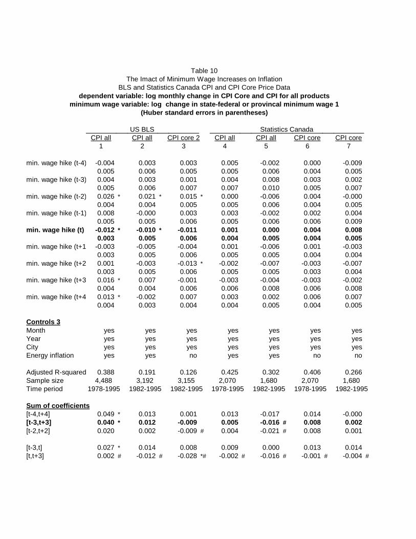
Table 10The Imact of Minimum Wage Increases on Inflation

BLS and Statistics Canada CPI and CPI Core Price Datadependent variable: log monthly change in CPI Core and CPI for all products

minimum wage variable: log change in state-federal or provincal minimum wage 1(Huber standard errors in parentheses)

Statistics CanadaUS BLSCPI coreCPI coreCPI allCPI allCPI core 2CPI allCPI all

7654321

-0.0090.000-0.0020.0050.0030.003-0.004min. wage hike (t-4)0.0050.0040.0060.0050.0050.0060.0050.0020.0030.0080.0040.0010.0030.004min. wage hike (t-3)0.0070.0050.0100.0070.0070.0060.005

-0.0000.004-0.0060.000*0.015*0.021*0.026min. wage hike (t-2)0.0050.0040.0060.0050.0050.0040.0040.0040.002-0.0020.0030.003-0.0000.008min. wage hike (t-1)0.0090.0060.0060.0050.0060.0050.0050.0080.0040.0000.001-0.011*-0.010*-0.012min. wage hike (t)0.0050.0040.0050.0040.0060.0050.003

-0.0030.001-0.0060.001-0.004-0.005-0.003min. wage hike (t+1)0.0040.0040.0050.0050.0060.0050.003

-0.007-0.003-0.007-0.002*-0.013-0.0030.001min. wage hike (t+2)0.0040.0030.0050.0050.0060.0050.003

-0.002-0.003-0.004-0.003-0.0010.007*0.016min. wage hike (t+3)0.0080.0060.0080.0060.0060.0040.0040.0070.0060.0020.0030.007-0.002*0.013min. wage hike (t+4)0.0050.0040.0050.0040.0040.0030.004

Controls 3yesyesyesyesyesyesyesMonth yesyesyesyesyesyesyesYearyesyesyesyesyesyesyesCitynonoyesyesnoyesyesEnergy inflation

0.2660.4060.3020.4250.1260.1910.388Adjusted R-squared1,6802,0701,6802,0703,1553,1924,488Sample size

1982-19951978-19951982-19951978-19951982-19951982-19951978-1995Time period

Sum of coefficients-0.0000.014-0.0170.0130.0010.013*0.049[t-4,t+4]0.0020.008#-0.0160.005-0.0090.012*0.040[t-3,t+3]0.0010.008#-0.0210.004#-0.0090.0020.020[t-2,t+2]

0.0140.0130.0000.0090.0080.014*0.027[t-3,t]#-0.004#-0.001#-0.016#-0.002*#-0.028#-0.012#0.002[t,t+3]

Notes:1 *=significantly different from 0 at the 5 percent level. #=sum of coefficients are significantly different from 0.02.2 The U.S core CPI is not available by city before 1982.3 Price controls include current and lagged monthly variables.

Appendix 1Descriptive Statistics on Inflation Measures 1

SampleSizeStd. DevMeanSeriesDataset(3)(2)(1)

U.S. BLS 1978-1995

4,4860.6060.418Food away from home4,4860.5230.455CPI all

1982-19953,1920.4820.290Food away from home3,1920.4140.285CPI all3,1550.4410.332CPI core 2

Canada's StatCan1978-1995

2,0700.7440.438Food at restaurants2,0700.4730.406CPI all2,0700.4310.406CPI core

1982-19951,6800.7170.339Food at restaurants1,6800.4260.301CPI all1,6800.3900.319CPI core

U.S. Chamber of Commerce1986-1993, Smoothed 3

3,0852.350.833Hamburger3,0823.030.456Pizza3,0653.630.539Chicken

1986-1993, Raw data3,0975.240.848Hamburger3,0975.180.519Pizza3,0978.240.658Chicken

Notes:1 BLS data is monthly at the city level. There are 27 cities up through 1986 and 15 after 1986. StatCan data is monthly at the province level. There are 10 provinces. Chamber of Commerce data is quarterly at the city level. There are 107 cities that are in the 1986 to 1993 sample period for at least 90% of the quarters.2 City-level CPI core index begins in 1982.

3 See text for more detail about the hamburger, pizza, and chicken products. Smoothed data eliminates temporary (less than 2 quarters) and large (> 5% quarterly change) spikes in the Chamber of Commerce price data through linear interpolation. Sample sizes vary between the smoothed and raw data because spikes that occur in the first two and last two quarters of the sample are thrown out.

Bibliography

American Chamber of Commerce Researchers Association. Cost of Living Index. LouisvilleChamber of Commerce: Louisville, KY. Various issues.

Baker, Michael, Dwayne Benjamin, and Shuchita Stanger. 1995. “The Highs and Lows of theMinimum Wage Effect: A Time Series-Cross Section Study of the Canadian Law.” Mimeo,University of Toronto.

Ball, Laurence and N. Gregory Mankiw. 1994. “A Sticky Price Manifesto.” Carnegie-RochesterSeries on Public Policy. p. 127-151.

Besley, Timothy. 1989. “Commodity Taxation and Imperfect Competition: A Note on the Effectsof Entry.” Journal of Public Economics. p. 359-367

Berk, R. 1990. “A Primer on Robust Regression.” In J. Fox and J. Long, eds., Modern Methodsin Data Analysis. Newbury Park, CA: Sage Publications.

Besley, Timothy and Harvey Rosen. 1994. “Sales Taxes and Prices: An Empirical Analysis.”Mimeo, Princeton University.

Brown, Douglas. 1990. “The Restaurant and Fast Food Race: Who’s Winning?” SouthernEconomic Journal. p. 984-995.

Card, David and Alan Krueger. 1995. Myth and Measurement: The New Economics of theMinimum Wage. Princeton, NJ: Princeton University Press.

Cecchetti, Stephen. 1986. “The Frequency of Price Adjustments: A Study of the NewsstandPrices of Magazines.” Journal of Econometrics. p. 255-274.

Delipalla, Sofia and Michael Keen. 1992. “The Comparison Between Ad Valorem and SpecificTaxation Under Imperfect Competition.” Journal of Public Economics. p. 351-368.

Green, David and Harry Paarsch. 1997. “The Effect of the Minimum Wage on the Distribution ofTeenage Wages.” Mimeo, University of British Columbia.

Gron, Anne and Deborah Swenson. 1996. “Incomplete Exchange-Rate Pass-Through andImperfect Competition: The Effect of Local Production.” American Economic Review. p. 71-76.

Grossman, Jean. 1983. “The Impact of the Minimum Wage on Other Wages .” Journal of HumanResources. p. 359-378.

Karp, Larry and Jeffrey Perloff. 1989. “Estimating Market Structure and Tax Incidence: TheJapanese Television Market.” Journal of Industrial Economics. P. 225-239.

Katz, Lawrence and Alan Krueger. 1992. “The Effect of the Minimum Wage on the Fast FoodIndustry.” Industrial and Labor Relations Review. p. 6-21.

Katz, Michael and Harvey Rosen. 1985. ”Tax Analysis in an Oligopoly Model.” Public FinanceQuarterly. p. 3-20.

Labor Canada. 1996. Employment Standards Legislation in Canada, 1995-1996. Ottawa: Supplyand Services Canada.

Lee, Jaewoo. 1997. “The Response of Exchange Rate Pass-Through to Market Concentration ina Small Economy: The Evidence from Korea.” Review of Economics and Statistics. p. 142-145.

Monthly Labor Review. Various January issues.

Neumark, David and William Wascher. 1992. “Employment Effects of Minimum andSubminimum Wages: Panel Data on State Minimum Wage Laws.” Industrial and LaborRelations Review. P. 55-81.

Parsley, David and Shang-Jin Wei. 1996. “Convergence to the Law of One Price Without TradeBarriers or Currency Fluctuations.” Quarterly Journal of Economics. P. 1211-1236.

Poterba, James. 1996. “Retail Price Reactions To Changes in State and Local Sales Taxes.”National Tax Journal. p. 165-176.

Stern, Nicholas. 1987. “The Effects of Taxation, Price Control, and Government Contracts inOligopoly and Monopolistic Competition.” Journal of Public Economics. p. 131-158.

Sumner, Daniel, 1981. “Measurement of Monopoly Behavior: An Application to the CigaretteIndustry.” Journal of Political Economy. p. 1010-1019.

Sullivan, Daniel. 1985. Testing Hypotheses about Firm Behavior in the Cigarette Industry.”Journal of Political Economy. p. 586-598.

Yang, Jiawen. 1997. “Exchange Rate Pass-Through in U.S. Manufacturing Industries.” Review ofEconomics and Statistics. p. 95-104.