Embed Size (px)
Citation preview

NASATechnicalMemorandum100010_
! tII
I| ,-
i Lecture Series in Computational
i Fluid DynamicsKevin W. Thompson
i
i (llASl-_II'l- 1000 10) LEC'I_S I_
CCEFU_,¢ICNAL FLUID D_ABICS (I_ASA) 110 pAvail: _-15 _-C AC6/B_ A01 CSCL 12A
August 1987
= National Aeronautics andSpace Administration
Z
N87-29_ 14
Uncla_
G3/64 00978C6
https://ntrs.nasa.gov/search.jsp?R=19870019781 2018-08-27T06:19:24+00:00Z

NASA Technical Memorandum 100010
Lecture Series in ComputationalFluid DynamicsKevin W. Thompson, Ames Research Center, Moffett Field, California
August 1987
RI/ .SANationAl Aeronautics andSpace Administration
Ames Research CenterMoffett Field. California 94035
Contents
Introduction
1 Conservation Laws, Wave Equations, and Shocks 3
1.1 Conservation Laws ............................... 3
1.2 Wave Equations ................................. 4
1.3 Continuous Analytical Solutions ....................... 5
1.4 The Breaking of Waves ............................. 671.5 Shock Waves ..................................
1.6 The Inviscid Burger's Equation ......................... 8
1.7 Expansion Shocks and the Entropy Condition ................ 9
1.8 Nonlinear Systems in One Dimension ..................... 10
1.9 Exercises .................................... 11
Finite Difference Solutions of Wave Equations
2.1
2.2
2.3
2.4
2.5
2.6
13
Basic Finite Difference Approximations ................... 13
A Brief Survey of "Traditional" Solution Methods ............. 16
2.2.1 First Order Upwind Methods ..................... 16
2.2.2 Explicit vs. Implicit Methods ..................... 17
2.2.3 Two Popular Second Order Schemes ................. 18
The Method of Lines .............................. 20
Dissipation and Discontinuous Solutions ................... 21
The Method of Lines in Two Dimensions ................... 24
Exercises .................................... 26
3 Stability Analysis
3.1
3.2
3.3
3.4
3.5
3.6
27
The Consistency Condition and the Lax Equivalence Theorem ...... 27
The Von Neumann Method for Stability Analysis .............. 29
3.2.1 Fourier Analysis and the Line.ar Wave Equation ........... 29
3.2.2 Fourier Analysis for Finite Difference Approximations ....... 30
3.2.3 Stability Condition for Numerical Methods ............. 31
Simple Upwind Schemes ............................ 32
Simple Centered Methods ........................... 32
The Lax-Wendroff and MacCormack Methods ................ 34
The Method of Lines .............................. 34
ii CONTENTS
4
6
3.7 Stability Analysis in Two Dimensions .................... 36
3.8 The Method of Lines in Two Dimensions ................... 37
3.9 Stability Limits for Fluid Dynamics Problems ................ 383.10 Exercises • • • • • • • • • • • • • • • • • • • • • • • • • • • • • • . , , , . . 39
A
Artificial Viscosity and Conservation Laws 41
4.1 Conservation Laws and Tensor Fields ..................... 41
4.1.1 Tensors ................................. 42
4.1.2 Coordinate Systems and Metric Tensors ............... 43
4.1.3 Combining Tensors ........................... 46
4.1.4 Covariant Differentiation ....................... 46
4.2 Fluids as Tensor Fields ............................. 48
4.3 Dissipation for Tensor Fields ......................... 504.3.1 Scalar Fields .............................. 51
4.3.2 Vector Fields .............................. 51
More on the Dissipation Coefficient ...................... 52
Dissipation in One Dimension ......................... 53
Dissipation in Two and Three Dimensions .................. 55
Coordinate Singularities ............................ 59
Dissipation for General Hyperbolic Problems ................ 59
Conservation Properties of Finite Difference Equations ........... 62Test Problems • • • • • • • • • • • • • • • • • • • • • • • • • • • • • . . . . . 64Exercises • • • • • • • • • - • • • • • • • • • • • • • • • • • • • • • • . . . . 69
4.4
4.5
4.6
4.7
4.8
4.9
4.10
4.11
Nonreflecting Boundary Conditions5.1
5.2
5.3
5.4
5.5
5.6
5.7
5.8
5.9
71
Waves in One Dimension ............................ 71
Nonreflecting Boundary Conditions in One Dimension ........... 73
Waves in Two Dimensions ........................... 75
Nonreflecting Boundary Conditions in Two Dimensions .......... 76
Numerical Solution of the Interior Problem ................. 77
Characteristic Equations for Fluid Dynamics ................ 79
Boundary Conditions for Fluid Dynamics .................. 81
Test Problems .................................. 83Exercises
• " • ° " • " ° • ° ° ° ° ° ° • " " ° " ° • " " ' • • • ° • • • • • ° • 94
The
A.1
A.2
A.3
A.4
A.5
Equations of Fluid Dynamics 95
Coordinate Geometries and Metric Tensors ................. 95
The Coordinate Invariant Fluid Equations .................. 97
Rectangular Coordinates ............................ 98
A.3.1 Connection Coefficients ........................ 98
A.3.2 The Fluid Equations withDissipation ................ 99
Cylindrical Coordinates ............................ 99
A.4.1 Connection Coefficients ........................ 100
A.4.2 The Fluid Equations with Dissipation ................ 100
Spherical Coordinates ............................. 101
.°,
CONTENTS m
Connection Coefficients ........................ 102
The Fluid Equations with Dissipation ................ 102
Bibliography105
List of Figures
1.1 Characteristic Diagram for Nonlinear Waves .................6
3.1 Stability regions for Runge-Kutta methods of order p ............ 35
4.1 Shock tube at step 60 ............................. 65
4.2 Spherical explosion at step 365 ........................ 67
5.1 Shock tube at step 100 ............................. 86
5.2 Spherical explosion at step 1000 ........................ 87
5.3 Homologous expansion at step 50 ....................... 89
5.4 Angled shock at step 0 ............................. 91
5.5 Angled shock at step 100 ........................... 92
5.6 Angled shock at step 200 ........................... 93
List of Tables
S.1 Reflections for Subsonic Shocks ........................85
Introduction
This text was written to accompany a series of lectures on computational methods for
fluid dynamics problems, which I gave in the Space Science Division at NASA Ames
Research Center in July and August of 1986. Each chapter in the text corresponds to a
particular lecture. Sufficient interest was expressed in the subject that Lynda Haines, the
User Services Manager of the Numerical Aerodynamic Simulator (NAS) Project, asked
me to prepare a series of videotaped lectures to be distributed along with this text.
Anyone interested in obtaining these tapes should contact NAS User Services at NASA
Ames Research Center, Moffett Field, CA 94035.
This lecture series covers the basic principles of computational fluid dynamics (ab-
breviated as "CFD" throughout). The lectures are designed to teach an inexperienced
person everything he or she needs to know to create a time dependent numerical model
of fluid flow, in one or more dimensions. I say "a model" because there is no unique
way to construct numerical models, and the number of such models which have been
constructed greatly exceeds the number of practitioners in the field.
As there are so many different approaches to simulating fluid flow, it is appropriate
to consider what will and will not be covered by these lectures. Lagrangian methods,
in which the computational grid moves with the fluid, will not be covered at all. Time
implicit methods will be mentioned, but not described in detail. Accelerated conver-
gence to steady states and boundary stability theory will be ignored. Finally, the great
majority of time explicit schemes, clever or otherwise, cannot be examined due to lack
of time, especially as some of them are quite complicated. This is not a survey course in
computational methods.
What will be covered are the basic concepts fundamental to every CFD scheme.
The emphasis will be on concepts and techniques which are simple, general, and have a
clear mathematical basis (criteria which exclude a great many methods in use!). While
the mathematical underpinnings are important, the usability of the methods is equally
important; therefore mathematical rigor will not be attempted, as the focus will be on the
concepts rather than their proof. Indeed, mathematically rigorous statements can seldom
be made about solution methods for CFD problems. Virtually all rigorous mathematical
work has been devoted to the simpler problems of linear systems or single nonlinear
equations. Fortunately, techniques developed for these simpler problems usually work on
the more complicated problems of nonlinear systems, even in the absence of mathematical
proofs that they should do so.
One standard of maturity for a field is the degree to which all conclusions follow
logically from a small number of basic principles. By this standard, computational

2 INTR OD UCTION
fluid dynamics is not a mature field. It has been characterized by a large collection
of complicated ad hoe methods. These lectures will try to achieve some maturity by
getting a widely applicable approach from a small number of basic concepts. In this
sense it departs from the "traditional" path in the CFD field, which has been to get thebest possible solutions to specialized problems.
Acknowledgment. I have performed this work while a National Research Council Re-
search Associate, doing research into astrophysics in the Space Science Division at NASA
Ames Research Center. I am indebted to the NRC, NASA Ames, and the Space Science
Division for supporting me in this work. I would also like to express my appreciation to
the NAS Project for sponsoring the production of the videotapes.

Chapter 1
,w
!
ii
Conservation Laws Wave
Equations and Shocks
This chapter deals with the general properties of hyperbolic systems of conservation
laws, of which the most frequently encountered example is probably the fluid dynamics
equations. It begins by defining what one means by "conservation," and describes the
close relationship between conservation laws and wave equations. We quickly discover
that the concept of a continuous function as the solution of a partial differential equation
is inadequate when we consider nonlinear equations, and are thus led to the concept of
shock waves as the required discontinuous solutions. We will also find that not all shock
waves which are allowed by conservation arguments are physically valid solutions, and
that only those shocks which satisfy an entropy condition may actually occur.
1.1 Conservation Laws
The equations of fluid dynamics are one example of the mathematical formulation of
conservation laws. The simplest one dimensional conservation law is a single equation,
describing a single conserved quantity, and may be written as either an integral equation
or as a partial differential equation. Suppose (in one dimension) that u is the density of
some conserved quantity per unit length, and f is the flux of u (i.e., the rate at which the
density u flows past a given x coordinate). The integrated density between two points
xl and x2, x2 < xl, satisfies [1]
d f_' u(x,t) dx = -[fCxl,t) - f(x2,t)].dt 2
(1.1)
If u and f are continuous functions of x and t, then in the limit as x2 _ xl - x, Eq. (1.1)
becomes
0u 0/=0. (1.2)a-T+
Eq. (1.2) is said to be in conservation form. More generally, any equation in which the
time derivative of a density plus the divergence of a flux equals inhomogeneous local

4 CHAPTER 1. CONSERVATION LAWS, WAVE EQUATIONS, AND SHOCKS
(i.e., non-derivative) source terms is in conservation form. In the case of (1.2), the flux
divergence is Of/Ox, and the source terms are zero.
The conservation form of an equation or system relates the time rate of change of
a density in a small volume to the flux of that quantity through the boundary of that
volume. Alternatively, one may recast the problem in terms of waves, and study the
propagation of wave amplitudes. The two approaches are nearly the same when applied to
single linear equations; however they are quite different, though still related, when applied
to nonlinear systems such as the fluid dynamics equations. The equivalent wave equations
are usually called characteristic equations in this context, while the wave velocities arecalled characteristic velocities.
1.2 Wave Equations
We begin by introducing the wave amplitude u, which is a function of the time t and the
spatial coordinate x. Suppose there exists a curve C in the xt plane, parameterized bythe variable a through the relations
x = x(a), t = tCa), (1.3)
where each point on C corresponds to a unique value of a. Then the rate of change of u
along the curve C is [2]du Ou Ou
do-_ -_t_ + OxX,,, (1.4)
where the subscripts denote derivatives with respect to a.
If u(x,t) is constant along C, we have
du
-0, (1.5)do
and C is called the characteristic curve, or simply characteristic, of u. Eq. (1.5) is calleda characteristic equation, and may be cast in different forms.
A common form for the characteristic equation is obtained by dividing (1.4) (with
du/da = 0) by to (implicitly assuming that to is never zero; we will assume that t(a) is
always an increasing function of a, as in t = e), giving
Ou Ou
c_--t+ aox = O, a = Xo/to = dx/dt, (1.6)
where a is the characteristic (or wave) velocity and is simply the slope of curve C in the
xt plane. If a is constant, Eq. (1.6) is a linear wave equation. If a = a(u) # constant,Eq. (1.6) is a nonlinear wave equation.
The conservation and wave equations for u are equivalent provided that the wave
speed a is given by
dIa- du" (1.7)

1.3. CONTINUOUS ANALYTICAL SOLUTIONS 5
If a = constant, the problem is linear and the solution is
u(x,t) = uo(x-at), where uCx,O ) = uo(x). (1.8)
The characteristics in the linear case are a family of parallel lines with constant slope
dx/dt = a, along each of which u = constant, although u varies from one line to thenext. The characteristics cover the entire xt plane in the region t >_ 0, implying that the
solution exists as defined for all x and t >_ 0.
The derivative du/da on the left side of (1.4) is often written with a - t, as in
du Ou dx Ou
d---[- Ot + d---[O---x' (1.9)
in which case it is called the total time derivative. The quantity du/dt in Eq. (1.9)
represents the time rate of change of u as measured at a point moving with velocity
dx/dt.
1.3 Continuous Analytical Solutions
Now consider the general case where a(u) is not constant. We know that u is constant
along each characteristic curve C in the xt plane, hence a(u) is also constant and the
characteristics are straight lines. However, as u varies from one characteristic to the
next, so does a(u), and the slopes of the characteristics also vary from one to the next.
Those characteristics which are initially separate will either diverge or converge, leading
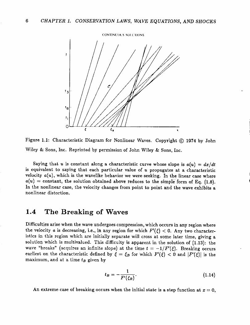
to behavior not seen in the linear problem. A typical characteristic diagram is shown in
Figure 1.1, reproduced from page 21 of the book by Whitham [1].
Let the initial value problem be given by Eq. (1.6) with u(x,O) --- f(x). Then for
each characteristic curve which intersects the x axis at x --- _ at time t = 0, u = f(_)
everywhere on that curve. The slope of a given curve is a(f (_)) = f(_) and is also known.
Each characteristic is therefore defined by a unique _ value, and has as its equation
x = + (1.10)
The complete set of _ values defines a whole family of characteristics, along each of which
the solution is
u = a = (1.11)Now let's check the solution. We find
1c_x 1 + F'(_)t' at
F(¢)1 + F'(_)t'
where the primes denote derivatives with respect to _, and therefore
au F(_)f'(_) Ou f'(_)
at 1 + F'(_)t' Ox 1 + F'(_)t'
(1.12)
(1.13)
and Eq. (1.6) is satisfied.
6 CHAPTER 1. CONSERVATION LAWS, WAVE EQUATIONS, AND SHOCKS
('ON[IN[;OUS ._(}I_UTION S
t
t3
tB
tl
0( (a x
Figure 1.1: Characteristic Diagram for Nonlinear Waves. Copyright (_) 1974 by John
Wiley & Sons, Inc. Reprinted by permission of John Wiley & Sons, Inc.
Saying that u is constant along a characteristic curve whose slope is a(u) = dz/dt
is equivalent to saying that each particular value of u propagates at a characteristic
velocity a(u), which is the wavelike behavior we were seeking. In the linear case where
a(u) = constant, the solution obtained above reduces to the simple form of Eq. (1.8).
In the nonlinear case, the velocity changes from point to point and the wave exhibits anonlinear distortion.
1.4 The Breaking of Waves
Difficulties arise when the wave undergoes compression, which occurs in any region where
the velocity a is decreasing, i.e., in any region for which F'(_) < 0. Any two character-
istics in this region which are initially separate will cross at some later time, giving a
solution which is multivalued. This difficulty is apparent in the solution of (1.13): the
wave "breaks" (acquires an infinite slope) at the time t = -1/F'(_). Breaking occurs
earliest on the characteristic defined by _ -- _B for which F'(_) < 0 and IF'(_)l is the
maximum, and at a time tB given by
tB= F'C_B)" (1.14)
An extreme case of breaking occurs when the initial state is a step function at x -- 0,
1.5. SHOCK WAVES 7
with
aCx, O)-- FCx) = {
al = a(ul), x > O, (1.15)
a2 = a(u2), X < O.
If a2 > al the solution breaks immediately.
A different result occurs of a2 < al. The wave undergoes expansion, and a continuous
solution results. At times t > 0 all values of F(0) between al and a2 spread out along a
fan of characteristics passing through _ = 0. This expansion fan is continuous, and must
satisfy (1.10) and (1.11), hence
x _x (1.16)a=_, a2< t <al,
and the complete solution for a is
a_, a_ < x/t;
a= x/t, a2 < X/t < al;
a2, x/t < a2.
The solution for u(x, t) is then obtained by inverting the known relationship a = a(u).
1.5 Shock Waves
In practice, the nonlinear wave equation we wish to solve represents a process whose
physical reality must be single valued, and the multi-valued solution produced by wave
breaking must be rejected. Yet solution (1.10)-(1.13) is valid up until the derivatives
become infinite, so we must modify our concept of a solution to include discontinuoussolutions which are single valued, and have a finite number of discontinuities. The formu-
lation of the wave problem as a partial differential equation is not valid for discontinuous
solutions, because the derivatives are defined only for continuous functions. However,
the integral formulation of conservation law (1.1) is valid even when u is discontinuous,and it is to this form we turn now.
Stable discontinuities in nonlinear waves are called shock waves, or shocks. On either
i _ side of the shock the solution is continuous and differentiable. If the shock is located atposition xo(t) and moves with velocity vs, where x2 < x_(t) < xx at time t, we may write
the integral equation for u as [1]
d fz_" . . d :_l
f(xu,t)- f(xx,t) - -_ J_] utx, t) dx + -_ J_[+ u(x,t) dx, (1.18)
| cz:o . . c o= dx + + c9 u(x,t) dx - u(x+,t)vo.(1.19)L+.
i=_
8 CHAPTER 1. CONSERVATION LAWS, WAVE EQUATIONS, AND SHOCKS
+ this becomes the shock jump conditionIn the limit as x2 _ x_-, xl --_ x 8
f2 - f, = v,(u2 - ul), (1.20)
where ]'1, ul are the flux and value of u on side 1 of the shock (taken to be the right
here), and fs, u2 are the values on side 2.
The shock jump condition may also be obtained by transforming the conservation
equation (1.2) to a reference frame in which the shock is at rest; i.e., which moves at a
velocity v, with respect to the original coordinate system. Integrating the transformed
equation over a small volume around the shock, and taking the limit as the volume goes
to zero, shows that the transformed flux f - uv8 must be continuous across the shock.
Thus fl - ulv, = fs - u2v,, which gives Eq. (1.20).
Rewriting (1.20) gives the shock velocity as
vs = f(u2)- f(ul) (1.21)u 2 -- u 1
In the weak shock limit where ]us- ul] << [u21 + lull we have us _ ul : u, and vo
Of/c3u -= a(u). Thus a sufficiently weak shock is a small discontinuity which travels at the
local wave velocity. A strong shock, however, has a velocity which is distinct from both
Ul and us. Note that Vo : a always for the linear wave equation, where a = constant.
1.6 The Inviscid Burger's Equation
Perhaps the most well known nonlinear wave equation is the inviscid Burger's equation
Ou i)u au c3 [u2"_
O---/+u_x =0, or -_-+Ozz _-2-) =0, (1.22)
which has f(u) = uS/2, a(u) = u. Burger's equation appears in most texts on nonlinear
hyperbolic equations, and in the inviscid form represents the velocity field of a gas of
non-interacting particles (such as a cloud of dust particles in a vacuum, or a zero pressure
gas).
The inviscid Burger's equation satisfies the general solutions obtained above. Its
solution for an initial discontinuity at z = 0, with u = u2 at x < 0, u = ul at x > 0, is
an expansion fan for us < u1:
u2, x/$ < u2;
uCx,t) = x/t, us < xl t < ul;
ul, ul < x/t;
and a shock wave for u2 > ul:
x < vst;
x > v_t;
(1.23)
(1.24)
1.7. EXPANSION SHOCKS AND THE ENTROPY CONDITION 9
where the shock velocity is obtained from (1.21):
1
v, (u2 + ul). (1.25)
The linear wave equation and the nonlinear Burger's equation represent special cases
of one dimensional planar fluid flow. If the fluid velocity v is constant with x, then
the continuity equation for the density reduces to (1.6), with u the density and a = v =
constant the fluid velocity. Density inhomogeneities are carried along by the flow without
distortion. However, if the pressure is spatially constant (c3p/Ox =- 0), then the velocity
equation reduces to the inviscid Burger's equation, with u the fluid velocity.
i
1.7 Expansion Shocks and the Entropy Condition
The preceding analysis found two different solutions to the nonlinear wave problem with
a step function initial condition. The case with a2 > al remains a step function, the dis-
continuity being a shock wave which propagates at the shock velocity given by Eq. (1.21).
The case with a2 < al breaks up into an expansion fan (which widens with time) adjoining
the constant states u2 and ul on either side.
The shock jump condition (1.20) says nothing about the breakup of a discontinuity
into an expansion fan. It is natural to ask if a discontinuity between two states with
a2 < al could also propagate as a shock, since the possibility is permitted by the jump
condition. Such a shock is known as an expansion shock, since it leaves behind a state of
decreased "density" u.
It turns out that expansion shocks are unstable. Small perturbations to an expansion
shock solution grow, destroying the shock. Compression shocks, on the other hand, are
stable. Stable shocks must satisfy the entropy condition [1], [3]
a2 > v, > ax, (1.26)
r, , • ,, r_
which means that characteristics cross at the shock front, and the slope of the shock
front line in the xt plane lies between the slopes of the characteristics which intersect
it from either side. Consequently no characteristic drawn in the direction of decreasing
t intersects a line of discontinuity, and every point in the plane can be connected by a
backward drawn characteristic to a point on the initial line at t = 0. In the case of the
inviscid Burger's equation, a = u, and v, = (u2 + ul)//2, which satisfies (1.26) only for
u2 > ul, as expected.
Expansion shocks are forbidden solutions for systems of nonlinear equations as well.
In the case of fluid dynamics, an expansion shock would cause the entropy of the flow to
decrease with time, and is forbidden by the laws of thermodynamics as well as stability
considerations. It is for this reason that criteria such as (1.26) are known as entropy
conditions.
10 CHAPTER 1. CONSERVATION LAWS, WAVE EQUATIONS, AND SHOCKS
1.8 Nonlinear Systems in One Dimension
In this section we consider systems of conservation laws of the form
U =
f
Ul
It2
, f=
Unk i !
(
fl
f2
f.k
(1.27)
where f is a vector flux and a function of the conserved densities which are the components
of the vector u. (Note that the term vector is used here in the linear algebra sense to
represent any set of unknowns, and not, for example, as a velocity vector.)
As in the previous section, let the states on either side of a shock be numbered 1 and
2 (1 for the right side, 2 for the left). The shock jump conditions are obtained by writing
Eq. (1.27) in integral form, and integrating over a small region containing the shock, as
in section 1.5. The n jump conditions are therefore
fi2 -- fil : I), (Ui2 -- Uil), i = 1,..., n, (1.28)
where fil _-- fi(Ul) is the ith flux on side 1 of the shock, and similarly for fi2. The shock
velocity v, is the same for all n jump conditions.
Eq. (1.27) can also be written in the form
0u A 0u 0u, _ 0u i (1.29)O---/+ Ox :0' or _+ aij-ff_-x =0, i=l,...,n,
j=l
where A is the Jacobian matrix of elements aij defined by
0I,aij -- au i. (1.30)
The system is defined to be hyperbolic if the matrix A has n real eigenvalues A_,
which we will order so that ,kl < ,k2 < .-. < _,,. The eigenvalues are the characteristic
velocities at which signals propagate in the medium described by (1.27). The character-
istic velocities are the slopes of the characteristic curves, as was the case for the single
wave equation. However, constancy of any wave amplitude along a characteristic curve
no longer implies constancy of the wave velocity along that curve, so the characteristic
curves need no longer be straight, and in general will not be. (A more detailed discussion
of the characteristic equations for nonlinear systems will be given in Chapter 5.)
The characteristic velocities determine an entropy condition for the nonlinear system,
which defines the class of allowed shock waves in a fashion analogous to Eq. (1.26). The
entropy condition for the nonlinear system, as given by Lax [3], is that for some value of
k, 1 _< k < n, the inequality
_k(U2) > 1), > _k(Ul) (1.31)
1.9. EXERCISES 11
must be satisfied.
In the case of fluid dynamics, the characteristic velocities are ,kl = v - c, ,k2 = v, and
,k3 = v + c, where v is the fluid velocity and c is the speed of sound. If the shock speed
is positive, Eq. (1.31) is satisfied by the case k = 3:
V2 -3t- C2 > V$ > Vl -_- el, (1/$ > 0), (1.32)
which means that right-moving sound waves on either side of the shock intersect the
shock. If the shock speed is negative, then
V2 -- C2 > V s > V 1 -- el, (v s < 0), (1.33)
which is the k = 1 condition, and implies that all left-moving sound waves intersect the
shock.
In either case, sound waves behind the shock (in the compressed region) travel faster
than the shock and catch up to it, while sound waves in front of the shock are propagating
more slowly than the shock and are overtaken by it. Thus the shock velocity is subsonic
relative to the post-shock state, but supersonic relative to the pre-shock state. Very
weak shock waves (characterized by very small shock jumps) are simply sound waves,
and travel at the speed of sound relative to the fluid. In this limit, the three velocities
in (1.32) become the same.
1.9 Exercises
1. Verify that the solution of (1.10)-(1.11) satisfies the integral equation (1.1), for the
linear case where F(_) = a = constant.
2. Find the shock jump condition for the equation
o(1)u2 +Ozz u3 =0.
Is it the same as (1.25) for Burger's equation? Does this result seem unusual?
Comment: A particular conservation law, such as (1.22), will give rise to an infinite
number of other equations upon multiplication by u to some power. The resulting
equations are equivalent for u a continuous function, but give rise to different shock
jump conditions. The correct jump condition may only be determined by reference
to the physics of the problem, i.e., by working with those quantities which are both
conserved and physically meaningful, such as mass, momentum, and energy.
, The general expansion fan u = (z-xo)/(t-to) is a solution to the inviscid Burger's
equation (1.22). Consider an initial value problem given by u = x/(l+t) for x < x0,
u = 0 for x > x0, at time t = 0. The point x0 is the initial shock location. Find the
solution for t > 0, including the shock location x, and shock velocity vs. (Hint: vo
is not constant with time.)
12 CHAPTER 1. CONSERVATION LAWS, WAVE EQUATIONS, AND SHOCKS
4. The fluid equations for a perfect gas in one dimension are
aT + (pv)= 0,
(pv) + (pv' + p) = 0,
where p is the mass density, v is the velocity, p = (7 - 1)e is the pressure, e is the
thermal energy density, and q is the (constant) ratio of specific heats (-- 5/3 for
an atomic gas). Find the shock jump conditions. Show that
P2
Pl
('t 4- 1)p2/pl 4- ('1- 1)
('l- 1)p2/Pl 4- ('l 4- 1)"
If P2/Pl can range from one to infinity, what values can the density ratio p2/pl take
on? (Hint: Although there are now three shock jump conditions, there is still only
one shock velocity.)
. Using the shock jump conditions derived in the previous problem, let pl -- pl -- 1,
vl = 0, "_ = 5/3, and p2/pl = 5. The speed of sound is c = _/_. Compute P2, v2,
and vo, draw a diagram of the pre- and post-shock characteristics, and show that
condition (1.32) is satisfied.
Condition (1.32) is condition (1.31) with k -- 3. For this problem, is condition
(1.31) satisfied for any other k?
Chapter 2
Finite Difference Solutions of Wave
Equations
The first chapter considered the general properties of conservation laws and wave equa-
tions in one dimension. This chapter will cover the basic concepts involved in the approx-
imate solution of wave equations by finite difference methods. The conservation laws of
interest are partial differential equations in one time and one or more spatial coordinates.
The numerical techniques to be described in this chapter will be oriented at first
toward the solution of the linear wave equation, in order to introduce the basic concepts
without obscuring them by the complexity encountered in solving nonlinear systems.
However, since the solution of nonlinear systems in more than one spatial dimension is
our ultimate goal, the implications of nonlinear systems for the solution techniques pre-
sented will be discussed after each technique is described. In Chapter 4 we will find that
consideration of the very general problem of multidimensional nonlinear systems with
shocks will determine the form of an artificial viscosity. This chapter will demonstrate
the need for artificial viscosity in problems with discontinuous solutions and will intro-
duce a form suited for the problems under discussion, but the fundamental justification
of the form will be deferred to Chapter 4.
2.1 Basic Finite Difference Approximations
We begin by considering a piecewise continuous function f(x), defined for all x. Ideally,
we would like to know the exact value of f for all x values, but in practice we will be
restricted to knowing f at a finite number of discrete points. Describing a function in
terms of its values at discrete points is known as discretization. For convenience sake, we
will discretize f(x) by recording its values at the set of grid points x_, spaced a uniform
distance Ax apart,
xi = lax, (2.1)
although in general one can have arbitrary grid spacing, which leads to more complicated
finite difference approximations. Denote the values of f at x_ by f_:
f, = f(x,). (2.2)
13
14 CHAPTER 2. FINITE DIFFERENCE SOLUTIONS OF WAVE EQUATIONS
Given the fi values, we need to approximate various derivatives of f at the grid points.
The starting point for all such approximations is the discrete Taylor's series [4],
fi+, = fi + nAx , + 2---_. dx 2 i +"" + m! dx,n +..., (2.3)
which holds for f(x) a continuous and infinitely differentiable function. If f(x) is not
continuous, this approximation breaks down and difficulties may occur. Techniques fordealing with discontinuous functions will be discussed later. For now we will assume that
all functions are continuous.
Setting n = +1, we see immediately that
_ 1 (/,+, _ f,) + (2.4)Ax1
- Ax (fi -- fi-1) -4- O(Ax). (2.5)
Eqs. (2.4) and (2.5) are called one sided difference approximations, and are the basis
for the low order upwind schemes to be discussed later. These one sided formulas are
formally of first order accuracy. The order of an approximation is given by the power
of the grid spacing Ax appearing in the leading error term, since the error in the ap-
proximation vanishes as that power of Ax in the limit as Ax _ 0. We can see that the
one sided approximations are first order accurate by solving for df/dxl_ in Eq. (2.3) withn:l:
df i 1 Axd2f] (_kx) 2 dSf (AX) m-1 dmfi_x -- ZXx (f_+'- f_)- _.. _x2 , - _. dx s , ..... m! dx '_ .... " (2.6)
For a sufficiently small Ax, the leading error term dominates, hence Eq. (2.4) is a first
order approximation to df/dx],, as is Eq. (2.5).
The first order approximations are useful in certain situations (such as at a bound-
ary, where symmetrically located data are not available), but their slow convergence
properties make them undesirable in most instances if more accurate approximations areavailable.
Replacing n by in in Eq. (2.3) and taking the difference of the expressions yields thefollowing result:
I d fl7"2"-- f_+'2nAx-fi-,, _ dxdf i + 3! dx 3 + 5! dx 5
from which we get the second order approximation
(nAx)S dr f+ 7-----_.dx' i +'"' (2.7)
df i fi+l -- fi-'dx -- 2Ax -4-O(Ax_). (2.8)
Note that Eq. (2.8) is not the only centered second order approximation. The quantity
T_, defined by Eq. (2.7), is a second order approximation to df/dx[, for any n value.
However, the error is quadratic in n, so the case n = 1 is clearly the best choice.
2.1. BASIC FINITE DIFFERENCE APPROXIMATIONS 15
We've seen first and second order approximations to df/dx. Higher order approxi-
mations may be constructed by taking appropriate linear combinations of the formulas
already obtained. For example, Eq. (2.7) gives an exact expression for the error terms
in the approximation T_. The following linear combination gives a fourth order approx-
imation to df/dxl_:
n2T_ - T_ df n 4 - n _ Ax 4 dS f n 6 - n 2 Ax 6 dr f l
T: =-- - d---xi- n2-1 5! dx s i- n----2- i 7[ dx r ,I ....(2.9)
n 2 - 1
The leading error term is again quadratic in n, and is minimized for n = 2 (note that n
may not be 1), giving
(2.10)
- - f,) - - f,-1)] + oCaz2), (2.13)
and which reduces to Eq. (2.12) for the case _¢= 1.
as the best fourth order approximation to df/dxli:
-- 1 [8(fi+x_fi_x)_(fi+2_fi_2)]_4_O(Ax4). (2.11)12Ax
Higher order approximations are obtained by computing lower order approximations
over different intervals nAx, then taking linear combinations of the results with coeffi-
cients chosen to cancel out the leading error term.
The above approach is an application of Richardson extrapolation, or the deferred
approach to limit [4]. Richardson extrapolation can be used to obtain improved, higher
order estimates of any quantity whose error is known to consist of a power series in some
discretization parameter. One computes the lowest order approximation to the quantity
using different discretization parameters (such as nAx in the above example), then takes
linear combinations of the two most accurate lower order approximations to obtain a
higher order approximation. In the above example, only even powers of the dlscretiza-
tion parameter appeared in the power series, so that a fourth order approximation was
obtained very quickly. In other circumstances, such as the first order approximations of
Eq. (2.6), all powers of the discretization parameter appear and more work is required
to obtain a given order of accuracy.
Another common example of Richardson extrapolation is Romberg's method for ap-
proximating definite integrals. One computes a sequence of trapezoidal approximationsto the integral, using different interval sizes, then takes linear combinations of the re-
sults to eliminate the leading error terms. The resulting approximation yields a much
more accurate approximation for a given amount of effort than does the trapezoidal
approximation by itself.
A similar analysis leads to the following formula for the second derivative of a function,to second order:
d2f = 1 (f,+l - 2f, + f,-1) + O(Ax2). (2.12)dx 2 i Ax 2
One also encounters diffusion terms, which may be approximated as
16 CHAPTER 2. FINITE DIFFERENCE SOLUTIONS OF WAVE EQUATIONS
2.2 A Brief Survey of "Traditional" Solution Meth-ods
Having mastered the basics of finite difference approximations, we will now attempt to
solve the one dimensional linear wave equation
au au
ot + a_x -- o, a -- constant, (2.14)
on a grid in the xt plane, at the points (x_, t"), spaced evenly in the x direction (x_ =iAx)
but" not necessarily in the t direction. Let U_ - U(x_, t") be the numerical approximation
to the exact solution u(x,t) at the grid points.
We are given a partial differential equation which relates the time variations in a
qua.htity u to its spatial variations, as well as initial data for all x values. The approximate
solution at a time At later is obtained from a numerical approximation to the differential
equation. Repeated applications of the numerical approximation yield solutions at a
sequence of advancing time steps.
The solution to the problem is completely defineCl once we have the differential equa-
tiofi and the initial data; hence the problem is called an initial value problem. A related,
but more complicated, problem is the initial boundary value problem, in which boundary
conditions as well as initial conditions over a finite spatial domain are specified. I will
return to the issue of boundary conditions in Chapter 5, but for now we will look at the
finite difference solution of wave equations over _an infinite domain.
The literature describing methods for solving wave equations and conservation laws is
very large, and a comprehensive examination of all such methods is not feasible. Instead
we will look a few representative and commonly used methods, chosen not only because
they illustrate the basic concepts of numerical solutions but also because they may be
applied to a wide variety of problems.
2.2.1 First Order Upwind Methods
The simplest and least accurate solution methods for the linear equation are the first
order "upwind" methods. Replacing the time and space derivatives in Eq. (2.14) by their
first order approximations yields four possible solutions:
V/n+1= V_ - a(V_ - V__l), (2.15)
U/n+l = V_ - u(Vi__ 1 - U/n), (2.16)
= - - U"+'), (2.17)u,"+1 u," oCv,"+' ,-1
-, ore-+' - u,-+_), (2.1s)_ u: +1=u_ _,.,where
At
o=._ (2.10)is called the Courant number, after Richard Courant, whose work in linear and nonlinear
waves and their solution forms the foundation for much of the field today.
2.2. A BRIEF SURVEY OF "TRADITIONAL" SOLUTION METHODS 17
At first glance these four approximations may seem equally valid-and they are from
the standpoint of the formal accuracy of the approximations out of which they were
constructed. However, two of them are guaranteed to be unstable for any time step
size At. Stability analysis will be deferred to Chapter 3, but for now it will simply be
stated that Eqs. (2.16) and (2.18) are unstable if a > 0, while Eqs. (2.15) and (2.17)are
unstable if a < 0. "Instability" means that the numerical solution grows exponentially
with the number of time steps, even though exponential growth is not a valid solution
to the given initial value problem.
The stability criteria for the upwind methods illustrate a very general property of
numerical solution methods, which can be stated as follows: The domain of dependence
of the numerical approximation to the solution of the differential equation must include
the domain of dependence of the original differential equation. For example, a right-
moving wave (with a > 0) has a solution whose time evolution at a particular point
is governed by the spatial variation of the wave to the left of that point-not to the
right. Therefore the numerical solution must make use of information to the left of the
grid point, which Eqs. (2.16) and (2.18) do not. One can define more precisely which
grid points should contribute to the solution by examining the characteristic curves of
the differential equation, but for now it will be sufficient to state that one may include
more points than are actually required, perhaps to improve accuracy, but the stability
requirements will depend in detail On the particular scheme chosen. Note that the upwind
scheme is so named because the points to be included in the first order approximation
are "upwind" from the current grid point.
Assuming that a > 0, we find that Eq. (2.15) is stable provided 0 < a < 1, while
Eq. (2.17) is stable for any a >_ 0. If the largest stable lal is a,,,_, we may use any At
value satisfyingAx
At < a,,_az la I • (2.20)
Thus approximation (2.15) is stable for At < Ax/lal, while (2.17) is stable for any At.
Similar stability criteria apply to approximations (2.16) and (2.17) when a < 0.
2.2.2 Explicit vs. Implicit Methods
The approximation of Eq. (2.15) is an example of a time explicit, or simply explicit,
method. An explicit method is one in which an unknown value at time step n + 1 appears
at only one grid point in the formula (e.g., U_+I), and is given explicitly in terms of the
previous values at step n. The approximation of Eq. (2.17) is an example of a time
implicit, or simply implicit, method. An implicit method is one in which the unknown
values of U at step n + 1 appear at more than one grid point in the approximation, and
are determined implicitly by a set of slmultaneous equations, rather than by a set of
independent explicit equations.
Explicit and implicit methods each have their advantages. Explicit methods are
much simpler to implement, as they do not entail the solution of simultaneous equations.
Explicit methods usually require much less time to evaluate, per time step, than implicit
methods, because the simultaneous equations inherent in the implicit schemes usually
18 CHAPTER 2. FINITE DIFFERENCE SOLUTIONS OF WAVE EQUATIONS
require lengthy calculations to solve. On the other hand, implicit methods are stable
for much larger time steps (often infinite, as above) than explicit methods. However,
the error in the time dependent numerical solution increases as some power of the time
step, so that in general an implicit scheme would require roughly the same time step as a
similar explicit scheme to achieve the same level of accuracy, but at a much higher cost in
computer time. Thus explicit methods are almost always preferable for time dependent
problems.
Nevertheless, there are situations in which implicit methods are preferable. One case
is the solution of "stiff" problems, which contain large characteristic velocities whose
corresponding effects are of minor importance. The time step for an explicit scheme is
limited by the largest characteristic velocity, whether or not the associated phenomena
play a major role in the solution. An implicit scheme may then be used with a time step
small enough to follow the phenomena of interest (such as convection), but much larger
than that dictated by the time scales of unimportant phenomena (such as sound waves).
Flows at very small Mach numbers fit into this category.
Another case in which implicit methods are useful is in steady state flow models. One
way to model a steady state flow problem is to pick a set of initial conditions and let the
problem evolve to an equilibrium state. The time dependent solution is of no interest,
and need not be accurate provided that the steady state solution obtained is correct.
Once again, a small number of computationally expensive steps may be more efficient
than a large number of inexpensive steps.
Implicit methods generally have to be tailored quite carefully to the problem at hand,
while explicit methods can be made very general. Thus from now on the discussion will
focus on explicit methods.
2.2:3 Two Popular Second Order Schemes
The first order upwind schemes suffer from two deficiencies. The first is low resolution.
An initially sharp profile (such as a step function) is smeared out or "diffused" over many
grid intervals as the solution progresses. This smearing tendency is known as numeri-
cal viscosity, and is a nonphysical effect (nonphysical because the original differential
equation was inviscid).
The second deficiency concerns the nature of the upwind stability criteria. In subsonic
fluid flow there is no simple upwind direction, as the flow has characteristic velocities
in all directions. A direct application of the upwind scheme will therefore be unstable,
unless the equations are put in characteristic form first, and each characteristic equation
approximated by the appropriate upwind form. The characteristic form is useful for
specifying boundary conditions, but is needlessly complex for other problems.
Finite difference schemes which make use of symmetrically located data points possess
stability criteria which are independent of the flow direction. One early attempt at a
symmetric method, which is still widely used, is the Lax-Wendroff scheme [5]. We start
with a Taylor's series approximation for U_ +1 about time t ", truncated after the secondorder term:
U: ÷1 = U: + At Ov " At_ 02U ". (2.21)Ot i + 2 Ot 2 i

2.2. A BRIEF SURVEY OF "TRADITIONAL" SOLUTION METHODS 19
(
Equation (2.14) may be solved by substituting -af/ax for au/at in (2.21), and using
Eq. (2.5) for the wave velocity. The result is the approximation
u,-+' = u,- - At + a ,i
where a = a(U) in general. Making the spatially centered, second order finite difference
approximations1
Ofax, 2Ax(fi+l- fi-1), (2.23)
a (aaf 1-_x _, -_x) i-- Ax 2 [a,+x/2(f,,x- f,)- a,-,/2(f,- f,-,)], (2.24)
gives an explicit solution to Eq. (2.14) which is second order accurate in time and space.
When applied to the linear wave equation, the Lax-Wendroff method gives
1 2. , U _U? +' = U_" - e(U_x - V__x) + _a (V2+ x - 2U_ + ,-x), (2.25)
with a given by Eq. (2.19), which has a stability criterion independent of the sign of a:
a AtLXz <- 1. (2.26)
The Lax-Wendroff method is easily applied to single one dimensional wave equations.
However, its extension to systems in one dimension, with an unknown variable vector
u and vector flux function f(u), entails the calculation of the Jacobian matrix 0f/0u
where the innocent-looking a appears in Eq. (2.22), a tedious if not impossible task.
MacCormack [6] came up with an apparently simpler method for the nonlinear sys-
tems case. MacCormack's method reduces to Eq. (2.25) for the linear wave equation,
but is not the same as the L:ax-Wendroff method for more complicated problems. The
MacCormack method solution to Eq. (2.14 i maybe written
AtU, = U? - A---x(f;+x- f?),
At - At - ,U?+I = U/t* 2_--x (f/ - ?i-1) 2-_-X (f_+l -- fin), (2.27)
= + At -(/' - ?,-1).
This is a two step explicit method which does not require the Jacobian of the flux
function. However, it is not a symmetric method: Eq. (2.27) uses a right direction one
sided approximation to Ofn/ax and a left direction one sided approximation to O'f/Ox.
One could have chosen the left direction approximation for the derivative of f" and
the right direction for f. The choice of direction for the terms is arbitrary, so long as
they are opposed, but the two possible choices will give slightly different results when
applied to the same nonlinear problem. MacCormack advocated switching the direction
of differencing at successive time steps in order to restore symmetry. Switching entails
cycling through 2"_ possible schemes in succession in m dimensions, which can lead to
complications as difficult as those of the Lax-Wendroff scheme.
20 CHAPTER 2. FINITE DIFFERENCE SOLUTIONS OF WAVE EQUATIONS
2.3 The Method of Lines
The preceding methods, while simple to formulate for single one dimensional wave equa-
tions, become quite complex and tricky to implement for multidimensional nonlinear
systems such as the fluid equations. The difficulties stem from the use of one-sided
difference approximations in the case of the upwind schemes, and from the simultane-
ous approximations of space and time derivatives in the Lax-Wendroff and MacCormack
methods. These difficulties can be avoided by the method o.f lines approach, which is
readily applicable to any time dependent partial differential equation solution.
We are given a set of partial differential equations in space and time, along with the
initial data at time t = 0. Approximating the spatial derivatives with finite difference
expressions in turn tells us how the solution changes in time at each grid point, allowing
:us to integrate the time derivatives to obtain the solution at a new time step.
More formally, suppose we have a system of equations describing the components of a
solution vector u. (For example, we might have u = (p, m, e), where p is the fluid density,
m is the momentum density, and e is the energy density.) If the time derivatives of the
components uj appear only in the first degree, then the system can always be written as
o_U
Ot -- Pu, (2.28)
where P is an operator involving any combination of the coordinates x and t, as well as
the unknown variables uj and their spatial derivatives, but no time derivatives of uj. In
the case of Eq. (2.14), u is a vector with only one component u, and Pu = -Of/Ox.
Now approximate all spatial derivatives in Pu with the appropriate finite difference
formulas, yielding the numerical approximation (PU)i (e.g., a spatially centered approx-
imation such as (PU), = -(fi+l - fi-1)/2Ax). Then we have a semi-discrete equation
for dUi/dt, the time derivative of U at grid point i:
dUidt - (PU),. (2.29)
in principle, any ordinary differential equation solution technique may be used to solve
the coupled set of ordinary differential equations in Eq. (2.29), as long as the stability
properties of the algorithm chosen allow reasonable step sizes At. Many such methodsare available.
The reduction of a system of partial differential equations to semi-discrete form,
followed by the integration of the system by an ordinary differential equation solver, is
known as the method of lines.
One effective integration method for Eq. (2.29) is the classical, four step, fourth order
2.4. DISSIPATION AND DISCONTINUOUS SOLUTIONS 21
Runge-Kutta method [4], written as:
1)
U_ 2)
U_ 3)
= U_ + _At(PU"),,
= U'_ + _At(PU(1)),, (2.30)
= U_ + At(PUO))i,
= U_ + _At(PU '_ + 2PU (1) + 2PU (2) + pU(S)), •
This method requires the storage of the o[_'ste_l_'U_, the current intermediate step U_ k),
and the running total of the sum of operators appearing in the last step.
The time error in (2.30) is O(At4). Since the maximum At is proportional to Ax
because of the stability criterion (given below), the time integration contributes an error
of O(Ax4). Thus the spatial approximations should also be fourth order accurate, orelse some of the effort involved in the time integration is being wasted. If the spatial
approximations are at best second order accurate (common in fluid problems), we should
use a second order time stepping scheme which requires less work to perform than (2.30).
The following four step, second order method is suited for such problems [7]:
1)
U_ 2)
U_ s)
= U'_ + ¼At(PU"),,
= U_. + _At(PUO)),,
= U'_ + _At(PU(2)),,
(2.31)
for the linear wave problem. If a second order centered approximation is made to Ou/Ox,
then a,_z -- 2V_; if a fourth order centered approximation is made, then e,_z -- 2.06.
(Note: when Pu is a linear operator, such as aOu/Ox, with a = constant-and only
then-Eq. (2.31) also gives a fourth order accurate time integration.)
2.4 Dissipation and Discontinuous Solutions
Consider the initial value problem
Ou Ou
0-'t- + aoxx = 0, a = constant > 0; (2.33)
U_ +i = U_ + At(puCs))_.
Not only does Eq. (2.31) require less storage than Eq. (2.30), but its simpler struc'ture
allows all four steps to be performed by one master loop, using a different coefficient for
- At in each iteration.
' Both the fourth order Runge-Kutta method of (2.30) and the second order method
i of (2.31) have the stability criterion At]a I = a_ <__amaz(2.32)
22 CHAPTER 2. FINITE DIFFERENCE SOLUTIONS OF WAVE EQUATIONS
(
u(x,O) = Uo(X) = I 1 x <_ O, (2.34)
( 0 x>O.
The solution is a step function of unit height, moving with velocity a. We would like to
solve this problem using the finite difference methods discussed so far.
This innocuous-seeming problem is in reality one of the most difficult wave problems
to solve numerically. The techniques previously described give uniformly poor results at,
say, a Courant number of a -- 0.5. The results fall into one of two categories: 1) solutions
which are monotonic but badly smeared, with the original discontinuity spread out over
many grid intervals, and 2) solutions which contain spurious oscillations, especially near
the discontinuity, but where the discontinuity is more sharply resolved than in category
1. The first order (upwind) methods yield the diffuse monotone solutions, while the
higher order methods yield the oscillatory solutions.
TheSe results are explained by the following theorem [8]: Any linear finite difference
scheme which is guaranteed to preserve monotonicity is no more than first order accurate.
This theorem is a major disappointment, as we would like to create high order solutionmethods which preserve the monotonicity of discontinuous solutions. The diffuse solu-
tions produced by first order methods are usually inadequate; however, highly oscillatory
solutions for discontinuous problems are equally inadequate. The theorem states that no
linear finite difference scheme will satisfy the conflicting requirements of monotonicity
and resolution. Therefore we must turn to nonlinear schemes for improvement. While
the properties of nonlinear schemes can seldom be analyzed analytically, much can be
accomplished by the careful blending of experience and linear theory.
We begin by examining more closely the first and second order approximations insemi-discrete form:
dUi 1
- _xta(Ui - Ui-1) (First order), (2.35)dt
_ 1 a(ui+l Ui-1) (Second order). (2.36)At 2
The choice of time integration is irrelevant for the moment, but Eq. (2.31) will do in
practice. Note that Eq. (2.35) may be written as Eq. (2.36) plus a correction term:
- -5( i+1 - U/-1) + (Ui+l - 2Ui + Ui-1) (First order). (2.37)dt At
(The above equation is in fact a general upwind scheme, which automatically switches to
the appropriate direction based on the sign of a.) The correction term may be thought
of as the finite difference approximation to the dissipative term
Oz At -_x '
with a diffusion coefficient defined by the Courant number a and the grid parameters
Ax and At. The added dissipation damps (i.e., prevents) the spurious oscillations which
2.4. DISSIPATION AND DISCONTINUOUS SOLUTIONS 23
would otherwise be generated by the second order centered difference approximation torl.l a,_)c3u/c3x. This particular choice of diffusion coefficient _ 2 -£T is exactly that required to
damp the oscillations completely, while a smaller value would not do so. This coefficient
also smears (diffuses) the solution badly, and reduces the overall accuracy of the approx-imation to first order. In the limit as Ax ---, 0 and At ---* 0, with a = aAt/Ax fixed, the
dissipative term vanishes (as it must, for the finite difference approximation to remain
consistent with the original inviscid equation), but it vanishes as a first order term.
The quest for a good nonlinear scheme may therefore be considered as a quest for a
good diffusion coefficient. We can write the equation to be solved as
a-7 = \ ax]'
with the understanding that _ is nonzero only because our grid intervals are nonzero.
In the limit as Ax and At vanish, _ must also vanish. Therefore we explicitly define
c_ At, in order that _ vanish in the appropriate limit. (Why do we not define _ o¢ Ax
instead? Because to do so leads to confusion and the violation of an isotropy condition in
multidimensional problems, as we'll see later. In addition, while At always has units of
time, the spatial grid parameter may have different units in different problems-angular
units, for example, in problems with cylindrical geometry. Thus it would be difficult to
come up with a general expression for _ which is proportional to the grid spacing.) We
also require that the relative sizes of the convective (a c3u/ax) and dissipative terms be
independent of the time step, as indeed they are in Eq. (2.37). These requirements are
met for a2
= kate, (2.39)
where k is a dimensionless, non-negative constant. Note that _ is never less than zero,
and is independent of the sign of a. The case k -- 1/2 recovers the monotone first order
result of (2.37). The case 0 < k < 1/2 reveals that while a linear scheme may not achievethe best of both worlds, it can achieve the worst: an oscillatory first order scheme!
Note that the above scheme works just as well on a nonlinear equation, such as
Burger's equation, where a(u) = u. Then a, _,and a = a(u)At/Ax are functions of
position, although At is not. In this case a c3u/ax should be written as of/ax, f = u2/2,
in order to ensure conservation and the correct shock jumps (as in Chapter 1).
Eq. (2.39) may be converted into a nonlinear scheme by defining
a_ (2.40),: = kathy,
where v depends on the local numerical solution U. We can define _ in such a way as to
satisfy v _< 1 always, to have v _ 1 near discontinuities and oscillatory regions, and to
vanish as a first order quantity in regions where U is a smooth, continuous function. In
finite difference form we write
0_/0 l _ xOz \ az] i Az _
24 CHAPTER 2. FINITE DIFFERENCE SOLUTIONS OF WAVE EQUATIONS
for which1
(2.42)
(2.43)
a? At
_i = kAt_v_, a_ = ai Ax"
Of the many possibilities we could pick for v_, one of the most useful is
Iu,+l - 2U, + u,-l[vi -- IUI+ x _ Ui[ + ]U_ - Ui-x[" (2:44)
This definition has vi = 1 if U_ is a i0cal_maximum or minimum. Thus _+1/2 will bea maximum only if Ui and U_+I are both local extremes, which is by definition a spurious
oscillation to be damped. Note that the local wave speed ai and Courant number ai
appear, so that the above prescription may be applied to the general case of spatially
varying wave velocities. The quantity aUlo,I la,I; hence the diffusion coefficient is
larger when the wave velocity is larger, which is as it should be, since the solution (and
spurious oscillations) will evolve more quickly in regions where a_ is large.
The constant k sets an upper limit to the diffusion coefficient, and is left as a free
parameter to be set by the user. Different problems will give the best results for different
k values. The choice k = 1/2 should eliminate spurious oscillations; however, in manycases k = 1/2 will be excessive, and a smaller value should be chosen.
The preceding analysis has focused on the choice of a second order central difference
approximation for the cgu/cgx (or Of/Ox) term. One could choose the fourth order
approximation (2.11), in which case the above scheme would still reduce to a first order
solution for _, _= 1, but which is not guaranteed to be monotonic. Nevertheless, one finds
in practice that those oscillations which do occur are more easily damped (i.e., requiresmaller k values) than is the case when second order approximations are made.
2.5 The Method of Lines in Two Dimensions
The extension of the preceding techniques to two or more dimensions is straightforward.We begin with a single conservation law in two spatial dimensions:
or
The two equations are
cgu Of ag
c9--[+ -_x + Oy =0' f = f(u), g = g(u), (2.45)
Ou Ou b i)u df b dgc3---[+ aox + Oy =0' a = d--_' = -_u"
equivalent. If a and b are constant, the solution is
(2.46)
ax + by )u(x,y,t) = u0 _-+ b' t , (2.47)
which is a wave moving at constant speed, with velocity components a in the x directionand b in the y direction.
2.5. THE METHOD OF LINES IN TWO DIMENSIONS 25
The second order semi-discrete approximation to Eq. (2.45} is
dUii _ _ fi+lj - fi-lj _ gij+l - gij-1 (2.48)dt 2Ax 2Ay '
in the absence of dissipation. The grid points are assumed to be uniformly spaced, with
x, : lAx, Yi = jAy, and U_] =-- U(x_, Yi, t'_) •
Dissipation is introduced by adding diffusive terms to Eq. (2.45) in the form
a--i+_ + a-_-a_\ a_J+_\ ay]'i
where _ ---} 0 as At --} 0, as before. We define _ in terms of the local Courant numberi
tTij,
Ay]'
and the largest local velocity component eli = max(]aij[, ]bij]):
• c.2._ij = kAt-s__Lu_j, (2.51)
o_j;_
where a useful (but not unique} definition for v,j is
( IV,+ly- 2v,y+ v,-xyl iv,y+,- 2v,y+ v,y_l]v,y = max _klV,+ly _ Viyl -_ IViy - Vi-ld]' [Viy+l - Viy] _ IVid - Vid-llJ "
(2.52)
The same definition for _ is used in both dissipative terms in Eq. (2.49). This unique-
ness in the definition of s is required by the transformation properties of scalar fields, a
subject which will be taken up in detail in Chapter 4.
The second order semi-discrete approximation to Eq. (2.49) is then
fi+ly -- fi-11 giy+l -- giy-1
2Ax 2Ay
1[_,+,/_(u,+ly- v,y)- _,_,/_y(u,y- u,_,y_]
1[_,_+l/,(V,., - U,y) - _,y_,/,CV, i - U,y_l)]
+ Ay------_ _ _
(2.53)
where1 1
#¢i+1/2i = _(tciy + tCi+lj), #¢0"+1/2 = 5( 'Y + _'i+')" (2.54)
The stability properties of this scheme are the same as for the one dimensional case of
section 2.3, and with maxa, y < a,_:,, for a as defined by Eq. (2.50), and a,na, as given
in section 2.3.

26 CHAPTER 2. FINITE DIFFERENCE SOLUTIONS OF WAVE EQUATIONS
2.6 Exercises
1. Using the fourth order approximation to df/dxl_ given in Eq. (2.9), compute thesixth order approximation.
2. Compute second and third order one sided approximations to dfldx]_, starting with
the first order one sided approximation of Eq. (2.6).
The following exercises are numerical solutions of the two initial value problems
Ou Of
0-_ + ox - O' f = au, a = l,
or
Ul(X ) : e-[("-o.15)/o.ll _,
u2(x) = _ 1 x<_0.25,
t 0 x > 0.25.
In all cases let Ax = 0.01, x_ =iAx, and compute the numerical solution Ui for grid
points i = 0 through 100. Define initial values for U_ for i = -2 through 102 from the
initial conditions, but do not recompute U-i, U-l, U101, or U102 at the new time steps.
(In other words, hold the boundary values fixed with time.) Compute 100 time steps
at a Courant number a = 1/2. At time step 100, plot the analytic solution ul(x - at)
or u2(x - at) as a continuous unmarked curve, and the numerical solution U/", n = 100,
as dots at the positions (xi,U_'), i = 0,..., 100. Use the computer to plot as well ascompute the results.
3. One sided (upwind) scheme (2.15) with ul and u2 as initial data.
4. Lax-Wendroff method (2.22) with ul and u2 as initial data.
5. Method of lines: scheme (2.31) with (PU), = -(fi+l - fi-1)/2Ax, using ul and u2as initial data.
.
Same as 3, but adding the dissipative term of (2.41) to the right hand side (i.e., to
(PV)_ as defined in problem 3), with _ given by Eqs. (2.42)-(2.44) and k =0, 0.2,and 0.5.
.
8.
Same as 6, but using the fourth order approximation (2.11) to OflOx.
Same as 3, but using Burger's equation in conservative form (1.22) and the initial
value problem of Exercise 3, Chapter 1. Compute the time step size at the beginning
of each time step according to At = aAxlU,,,_,, where U,_ is the largest absolute
value of the numerical solution (maxi l°° Iu/-i) on the grid at the beginning of the
current time step. The left boundary condition must now be changed to one of
antisymmetry, given by U-1 = -U1, U-2 = -U2. Does the numerical solutionmatch the analytical solution?

Chapter 3
Stability Analysis
Chapter 2 presented several approximate finite difference solutions for one dimensional
conservation laws. The criteria used to select an appropriate technique are stability,
accuracy, and efficiency. Of these stability is the most important, as the formal accu-
racy and efficiency of a method are irrelevant if the method is unstable in practice. The
stability limits for the methods in Chapter 2 were stated without proof. In this chap-
ter I will present a general technique for determining the stability of finite difference
approximations for wave equations.
3.1 The Consistency Condition and the Lax Equiv-
alence Theorem •
The partial differential equations we wisht° solve may be written in the general form
0__uu= Pu, (3.1)at
where P is an operator which acts on u to give its time derivative. The quantity Pu may
be nonlinear and contain any combination ofpowers of the spatial coordinates, time,
or unknown elements uk, or any spatial derivatives of these combinations, but may not
contain time derivatives of u.
As in Chapter 2, we consider only the pure initial value problem, for which the initial
data are given, and the time dependent solution is to be obtained, over an infinite spatial
domain with no boundaries or boundary conditions.
Replacing the spatial derivatives in P with suitable finite difference approximations
yields the semi-discrete approximation
dU, _ (PU),, (3.2)dt
where Ui is the approximate solution for U at the ith grid point.
Given data at time level t", we integrate Eq. (3.2) to time level t n+l = t _' + At. Thus
the new value of U_ +1 is some function of the old values U_+ k, k = -co,..., co. The
27
28 CHAPTER 3. STABILITY ANALYSIS
functional relationship between the new and old values may be written
U_ '+I = C(At)U_', (3.3)
where the operator C(At) acts on Ui and depends on At.
We know from section (2.1) that the quantity (U_ +1 - U_)/At is an approximationto the time derivative of Ui, hence
C(at)U"-U"At
must be an approximation to PU.
The consistency condition therefore requires that
it{c t,,} pIAt - P U,(t) _0 as At-v0, (3.4)
where Ilfll is any valid norm=of f and I is the identity operator [5].
The consistency condition looks imposing, but it is simply a formal statement of an
intuitively meaningful concept, namely that the finite difference approximations which
are used in the numerical solution of a differential equation must yield that equation in
the limit as all grid spacings go to zero (i.e., as Ax --. 0 and At --, 0 for the methods ofChapter 2).
The consistency condition is automatically satisfied by any one-to-one replacement of
derivatives by valid finite difference approximations, so the insistence on consistency may
seem redundant. However, we saw in Chapter 2 that dissipative terms were required in
the finite difference solution to discontinuous problems, even though these terms do not
represent finite difference approximations to derivative terms appearing in the original
differential equations. Thus an approximation containing these added dissipative terms
must be defined in such a way that the dissipation vanishes in the limit of zero grid
spacing in order to retain consistency (otherwise our finite difference method is solving a
problem different from the one whose solution we want). The dissipative terms in section
2.4 vanish as At _ 0, because g 0¢ At. If we had defined g so that g # 0 as At _ 0,
Ax --, 0, then the approximation would have been inconsistent, and guaranteed not toconverge to the correct answer in this limit.
The definition of consistency given above leads to the Lax Equivalence Theorem [5]:
Given a properly posed initial-value problem and a finite difference approximation to it
that satisfies the consistency condition, stability is the necessary and sufficient conditionfor convergence.
The proof of the theorem assumes P to be a linear operator, but in practice the same
result is observed to hold for nonlinear systems as well, provided the dissipation is chosenproperly.
Having established that stable and consistent schemes will converge to the correct
answer, we proceed next to define and analyze the stability of finite difference approxi-mations.
3.2. THE VON NEUMANN METHOD FOR STABILITY ANALYSIS 29
3.2 The Von Neumann Method for Stability Analy-
sis
According to Eq. (3.3), the operator C(At) advances the solution from time t to time
t + At. Thus initial data U ° yield data at time t n = nAt through the repeated application
of c(At), .....U_'--[c(At)l"v °. (3.5)
A scheme is stable ifthere exists a r > 0 such that the set of operators [C(At)] n is
bounded for 0 <_ At _< r. In other words, the numerical solution may not grow without
bound (provided that the correct solution does not). Conversely, a numerical scheme
which is unstable will exhibit unbounded growth, and this growth is virtually always• ..... L -
exponential.
Note that computing a bound for [C(At)]_ isnot trivial,as C(At) isan operator, not
a number. Fortunately, a straightforward{echnique for transforming the operator C(At)
into a number does exist,when C(At) is a linearoperator. The technique isknown as
the Von Neumann method and is described below.
.... _ . _.i ,_._ _i ' !.
3.2.1 Fourier Analysis and the .Linear Wave Equation
We consider once again the linear wave equation
Ou Ou (3.6)0-7 + aoxx = 0, a = constant,
!and examine the behavior of the numerical solution for u. Fourier analysis turns out
to be a convenient tool for this examination. The Fourier transform of a function ](x)
is the frequency spectrum of the function, f(w), and is a function of the frequency w.
If f = f(x,t) and we take the Fourier transform of the x dependence, the spectrum is
f(w,t). If in turn f(w,t) is a monotonically increasing function of t for some frequency w0,
f(x, t) will be an unbounded function, since the frequency component w0 grows without
! bound.
i The Fourier transform of the x dependenters:_ :_ of,. a function u(x,t) may be written
1 e-'WZu(x,t) dx =- _(w,t), (3.7)
and is finite if u(x, t) _ 0 sufficiently quickly as x _ _c_, which we will assume through-
-" out.
i The derivative Ou/cgx transforms according to
{0_ )} 1 _ _x (3.8)i oo
which is obtained upon integration by parts.=
|
30 CHAPTER 3. STABILITY ANALYSIS
Taking the Fourier transform of the linear wave equation (3.6) gives
a--t -t- {waft = O. (3.9)
Notice that Eq. (3.9) is an ordinary differential equation for any particular choice of
w. The effect of the Fourier transform has been to replace a single partial differential
equation with an infinite number of ordinary differential equations.
The solution of Eq. (3.9) is
and therefore
_@,t) = e-'_'"',_(w,o), (3.1o)
_@,t)_@,0) = 1. (3.11)
Although the phases of the components of the frequency spectrum change with time,
their magnitudes do not. Indeed, this is the behavior we would expect, since we know
the solution to be a traveling wave of constant shape.
3.2.2 Fourier Analysis for Finite Difference Approxlrnations
Previously we have taken Ui" to be the numerical approximation to the exact solution at
the point (x_, tn). For the remainder of this chapter, we will adopt a slightly different,
but equivalent, interpretation, and assume that Uik is a function defined by
,, )j,°U_+k _ U(x -I- kAx,t (3.12)Zi'
which we happen to sample at discrete points. Thus any derivative approximation, suchas
ov . v_+l- u?___ v(x + Ax,t") - U(=- Ax, t-)lOx i _ 2Ax = 2Ax I,,' (3.13)
is also a continuous function, and we may compute its Fourier transform.
Assuming Ax to be a fixed constant, we have
z{u(x,t)}=O, (3.14)
7U(x + kAx, t)} = eikeO, _ =_-wax. (3.15)
The variable ( is referred to as the dimensionless frequency, and is an angular quantity(hence dimensionless).
We can now compute the Fourier transforms of finite difference approximations. Let
A--6(")U,_== , be an ruth order approximation to cgU/cgxli. Then we represent the one sided
approximations by
6(I)-U_ = Ui - Ui-1, 6(1)+Ui= Ui+i - Ui, (3.16)
3.2. THE VON NEUMANN METHOD FOR STABILITY ANALYSIS 31
and the centered approximations by
_5!2)U' = 1_(U,+, - Ui-,), (3.17)
_C,)v,, : 118(u,+, - U,_l) - (v,+, - v,__)]. (3.18)
The second derivative, i)2U/cgx21_ is approximated by 1 2 ('_)U_, to order m, and we
have
6_ {_)U_= U_+l - 2U_ + U__l.
The transforms are
f{6_X)-V,} = (1- e-'_)_ r, 7{6,(*)*U,} = (e '_- 1)Lr,
_{6_)v,} = (isin ¢)0,
7{6(4)U_} = il[8sin _- sin(2_)]0,
r{_: C2)v,}= -4sin_(_/2)0.
(3.19)
(3.20)
(3.21)
(3.22)
(3.23)
3.2.3 Stability Condition for Numerical Methods
We can now state the Von Neumann stability condition for numerical approximations to
the linear wave equation. All one step linear finite difference solutions to the linear wave
equation (3.6), implicit or explicit, can be written as
oo oo
l_v_'= _ r_v?,_, (3.24)k=-oo k=-oo
where the lk and rk are constants. Taking the Fourier transform of Eq. (3.24) gives
from which we see
(3.25)
0 "+' =g(¢)O", (3.26)
_._=-oo rk eit_ (3.27)
where g(_) is known as the Fourier amplification .factor.
The Von Neumann stability condition is the following [5]: Stability of finite difference
approximation C3.$4) requires that g(_), as defined by Eq. (3.$7), satisfy
[g(_)]_l, for all,in -Tr< _<_r. (3.28)
Otherwise the numerical solution grows exponentially with the number of time steps. _
The preceding formalism may appear complicated, but is simple to implement in
practice, as the following examples show.
1A more general condition allows for exponential growth when such growth is a valid solution, and
requires g(_) < 1 + O(At) [5]. This situation occurs when a source term bu is added to the right hand sideof (3.6). For most problems condition (3.28) is sufficiently general, and will be used in these notes.
32 CHAPTER 3. STABILITY ANALYSIS
3.3 Simple Upwind Schemes
Let us first consider the upwind schemes of section 2.2.1.
Eq. (2.15) is
0 "+1 -- [1 - a(1 - e-ie)]0 ",
The Fourier transform of
(3.29)
g(() = 1-o(1-e-'_), (3.30)
= 1 - a(1 - cos () - igsin _. (3.31)
Multiplying Eq. (3.31) by its complex conjugate gives the square of the absolute magni-tude of g as
[g(()[2 _- 1 - 4a(1 - a)sin2((/2). (3.32)
The worst case has _ -- _r, for which
Ig(r)[ 2 : 1- 43(1- a) _< 1, (3.33)
a(1 - a) > O, (3.34)
and we must have 0 _ a < 1 for approximation (2.15) to be stable. A similar calculation
shows that the stability bounds for approximation (2.16) is -1 < a < 0. Thus the
stability of the explicit upwind schemes depends on the sign of the velocity a.
Consider next the implicit upwind scheme of Eq. (2.17). Its Fourier transform is
_n+l ---- 0n __ a(1 -- e-'_)0 "+', (3.35)
g = 1 -- a(1 -- e-'_)g, (3.36)
1
g(_) = 1 + a(1 - cos _) + iasin _' (3.37)
ig(5)l2= 11 + 43(1 + a) sin2(_/2)" (3.38)
Again the worst case occurs at _ = _r, and the condition Ig(_)] -< 1 implies
o(1 + o) _>o, (3.39)
and the method is stable for any a >__0, Similarly, approximation (2.18) is stable for anya<0.
3.4 Simple Centered Methods
The simplest centered method we can have is the approximation
1 n
u,"+1= u,- - _oCUhl- u,__,). (3.40)
3.4. SIMPLE CENTERED METHODS 33
1[i_!!i
The Fourier transform of (3.40) gives
g(f)---- 1-iasin_, (3.41)
Ig(OI== I+ o=sin2f, (3.42)
so that approximation (3.40) is unconditionally unstable!
In Chapter 2 we found a dissipative term which, when added to the simple centered
difference approximation, produced an upwind scheme which we now know to be stable
for suitable time steps. The dissipative term is given in Eq. (2.37), and a first order time
integration of (2.37) is
(3.43)
The Fourier transform of (3.43) gives
9(f) = 1 -[,_1(1- cosf) - iasin _, (3.44)
la(01== 1 q- 4(a 2 --]a[) sin2Cf/2), (3.45)
and the stability condition is
o=-Iol < 0, (3.46)
which is satisfied for [a I < 1, and is independent of the sign of the velocity, unlike the
original one-sided schemes.
We conclude that adding dissipation to a centered scheme which is originally unstable
may produce a stable scheme. Thus we now consider a more general scheme of the form
1 , U'*u?+1= u? - o(V?+l- u"_,) + 5,_(v;+, - 2u? + ,_1), (3.47)
where a = _At/Ax 2 and _ is a constant diffusion coefficient, as in Eq. (2.38). The
Fourier transform of Eq. (3.47) gives
g = 1 - iasin _- 2ct(1- cos _), (3.48)
Ig(g)l2 = 1 - 8asin=({/2) + 1632 sin4({/2) + a 2 sin 2 {-
The condition ]g({)l <- 1 yields the equation
(3.49)
f(_) = [2a-a 2+(a 2 -432)sin2(_/2)]sin_(_/2) >0 for all_. (3.50)
Eq. (3.50) specifies a relationship between a and a. Analyzing (3.50) in detail serves
no purpose for the present, but for a given a it puts lower and upper limits on the range
of a values which will lead to a stable approximation, and it defines a maximum value
of [a] above which any approximation will be unstable for any value of a.
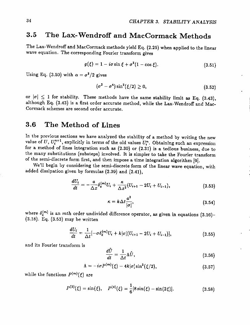
34 CHAPTER 3. STABILITY ANALYSIS
3.5 The LaxoWendroff and MacCormack Methods
The Lax-Wendroff and MacCormack methods yield Eq. (2.25) when applied to the linear
wave equation. The corresponding Fourier transform gives
g(_) = 1 - iasin_ + as(1 - cos _). (3.51)
Using Eq. (3.50) with a = as�2 gives
(a s - 04) sinS(_/2) > 0, (3.52)
or [cr[ < 1 for stability. These methods have the same stability limit as Eq. (3.43),
although Eq. (3.43) is a first order accurate method, while the Lax-Wendroff and Mac-Cormack schemes are second order accurate.
3.6 The Method of Lines
In the previous sections we have analyzed the stability of a method by writing the new
value of U, U/"+I, explicitly in terms of the old values U/". Obtaining such an expression
for a method of lines integration such as (2.30) or (2.31) is a tedious business, due to
the many substitutions (substeps) involved. It is simpler to take the Fourier transform
of the semi-discrete form first, and then impose a time integration algorithm [9].
We'll begin by considering the semi-discrete form of the linear wave equation, with
added dissipation given by formulas (2.39) and (2.41),
dV,L lgdt d_Cm)Vi "[- _-_X 2 (v/+l -- 2vi + Vi-1)' (3.53)
a s
= kAt_l, (3.54)
where _("_) is an rnth order undivided difference operator, as given in equations (3.16)-(3.18). Eq. (3.53) may be written
dUi 1_ [-o6c,_lv, + klol(V,÷l- 2u, + v,_l)],
dt At (3.55)
and its Fourier transform is
d0 1 A
- AU,dt At
A = -iaP("_)(_) - 4klo[ sinS(_/2),
while the functions p(m)(_) are
(3.56)
(3.57)
pCS)(_) = sin(_), P(')(_) = l[8sin(_) -sin(2_)]. (3.58)
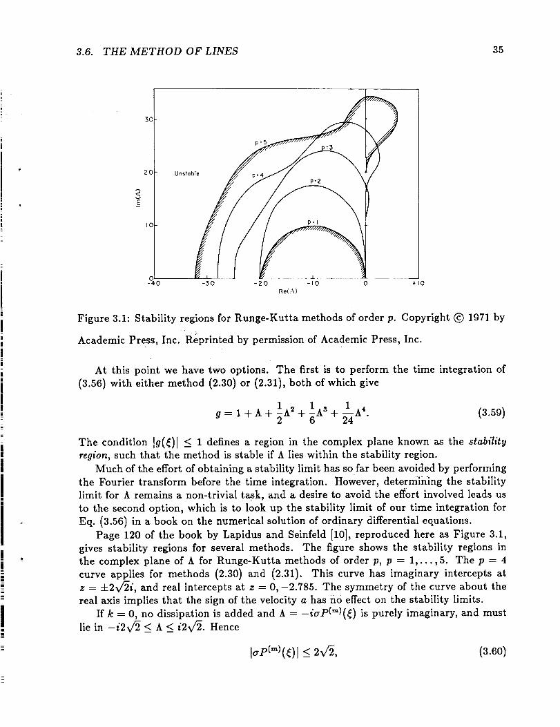
3.6. THE METHOD OF LINES 35
3O
2O
IO
0 L-41 30 20 I0 0 "t-I0
Re(A)
Figure 3.1: Stability regions for Runge-Kutta methods of order p. Copyright © 1971 by
Academic Press, Inc. Reprinted by permission of Academic Press, Inc.
At this point we have two options. The first is to perform the time integration of
(3.56) with either method (2.30) or (2.31), both of which give
1A _g= I+A+ h 2+6 + 1A4"24 (3.59)
The condition [g(_)] _< 1 defines a region in the complex plane known as the stability
region, such that the method is stable if A lies within the stability region.
Much of the effort of obtaining a stability limit has so far been avoided by performing
the Fourier transform before the time integration. However, determining the stability
limit for A remains a non-trivial t_k, and a desire to avoid the effort involved leads us
to the second option, which is to look up the stability limit of our time integration for
Eq. (3.56) in a book on the numerical solution of ordinary differential equations.
Page 120 of the book by Lapidus and Selnfeld [10], reproduced here as Figure 3.1,
gives stability regions for several methods. The figure shows the stability regions in
the complex plane of A for Runge-Kutta methods of order p, p -- 1,...,5. The p -- 4
curve applies for methods (2.30) and (2.31). This curve has imaginary intercepts at
z -- +2V_i, and real intercepts at z -- 0,-2.785. The symmetry of the curve about the
real axis implies that the sign of the velocity a has no effect on the stability limits.
If k = 0, no dissipation is added and A = -iaP(m)(_) is purely imaginary, and must
lie in -i2v_ < A < i2v/2. Hence
<_2v , (3.60)

36 CHAPTER 3. STABILITY ANALYSIS
and the maximum allowed value of a is determined by the largest value of P('_)(_).
We quickly determine that P(_a}z = 1, and P_)x = 1.3722, hence a _< 2v_ for stability
if a second order approximation to Ou/c3x is made, and a < 2.0612 if a fourth order
approximation is made. (In both cases k = 0. Dissipation will decrease the stability
limit even though it improves the quality of the solution.)
At the other extreme we consider the purely dissipative problem, with a = a = 0,
and replace kla I in (3.57) by _At/Ax 2. Then h = -4_a-_sin2(_/2), and -2.785 <_
h _< 0, from which we see that _At/Ax 2 < 0.6963 for stability. In real diffusion or heat
conduction problems, where _ is some nonzero function of the solution u, the maximum
stable time step is proportional to the square of the grid spacing. Reducing the grid
spacing by a factor of two decreases the allowed time step by a factor of four. A finely
spaced mesh may therefore require a prohibitively small time step for an explicit scheme
to be stable, which suggests that an implicit scheme might be more efficient, though
considerably more difficult to implement.
For the added dissipation we are considering here, _At/Ax 2 = k[a[, which vanishes
as a ---* 0, so we cannot obtain a purely dissipative problem while a is nonzero. However,
if a is sufficiently small, we can make k large enough that the second term of Eq. (3.57)
dominates over the first, and we may conclude that k is restricted by the requirement
kla I <_ 0.6963 for stability.
A general expression relating the maximum value of k as a function of the Courant
number a probably cannot be derived analytically, but is not really necessary. If lal does
not exceed roughly half of its upper limit, one can in practice make k large enough to
damp any oscillations. The practical condition is to compute the time step from
at = axe, (3.61)
where a is a Courant number which is less than the maximum value, and to set k to an
optimum value obtained by experimentation (e.g., lal = 1, k = 0.3).
3.7 Stability Analysis in Two Dimensions
Stability analysis for two or more dimensions is very similar to the one dimensional case,
and we can use the one dimensional results with only slight modifications. We start
with the Fourier transform in two dimensions (x, y) of a function u(x,y, t), which maybe defined
_'{u(x,y,t)} = _ dx dye-iC_x*+_'_)uCx, y,t) =- ¢_(wx,wv,t ). (3.62)O0
It follows that
where
+ mz ,y + = eim e'n"O, (3.63)
=--wzAz, 77 = w_Ay. (3.64)
3.8. THE METHOD OF LINES IN TWO DIMENSIONS 37
As in Eq. (3.24), any one step linear finite difference solution to the linear equation
Eq. (2.46) may be written
oo oo
TTr_-t-1 n (3.65)s_,v,+k,j+,= _ rk,VLk,j+,.k,|=-vo k,l=-oo
where the ski and rkl are constants.
We take the Fourier transform of Eq. (3.65) and define the amplification factor g(_, ,7)
by
0-+, = g(_,,,)O-. (3.66)
The Von Neumann condition is then
i9(_,.)I<-I, --_r_<_ <_ r, -_ <__ _<_r. (3.67)
3.8 The Method of Lines in Two Dimensions
As in the one dimensional case of section 3.6, we write the differential equation in semi-
discrete from first,
dUij
dta _(,_)rT.. b__6('_)U..
Ax_Z v,_ Ay v 'JI¢
n 2u,_ + u,_l_) + 2u,i + u_i-_),+_-_(u,+,_ - h-_y_(v,i+, - (3.68)
i c 2n = kAt--, e = max(lal, Ibl),
o"
i with a to be defined below, and then take its Fourier transform to get
i dr} 1 AU (3.70)"-d7-- _
# a_t
ib_--_fP ('_) 4_ At sin'(_/2)- 4_A_-_2 sin_(rl/2 ). (3.71)
. A=-,_-xP '(_)- _Y (,7)- _x 2 Y
(m"
Once again we simply look up the stability region for A in the complex plane for the
.....(3.60).,
lal Ibl% AtP (m) < 2V_. (3.72)Ax + Ay] ""_ -
particular time integration method we use. If either method (2.30) or (2.31) is used, we
get g(_, rl) as given by Eq. (3.59), but with A as defined above in Eq. (3.71).
Consider now the case of no dissipation (_; -- 0). Then A is purely imaginary, and
achieves its extreme values for r/= q-_ such that P('_)(_) is maximized. Since the extreme
values of A on the imaginary axis for which the method is stable are -I-i2V_, we see that
38 CHAPTER 3. STABILITY ANALYSIS
(The absolute value signs are used in (3.72) to cover the case where a and b have opposite
signs, in which case the most extreme A occurs for p(m)(_) and P("_)(r/) maximum in
magnitude but of opposite sign.) If we define the Courant number in two dimensions by
= (lol Ibl t, (3.73)a \Az + Ay]
we recover the familiar stability limit of (3.60), written as
aP(_a)__<2V/2. (3.74)
If m = 2, a < 2V_; if m = 4, a < 2.0612. We select a stable value for a and compute At
fromO
At -- I_1 + Ibl" (3.75)Az Ay
The case where dissipation dominates leads to the result
_ + ,_At _<0.6963, (3.76)
which for _ as defined by Eq. (3.69) puts an upper limit on k for any given At, or vice
versa:
3.9 Stability Limits for Fluid Dynamics Problems
As we will see in Chapter 5, the three equations of one dimensional fluid dynamics may
be transformed into an equivalent set of coupled nonlinear wave equations. The wave
velocities are the characteristic velocities of the system, namely v - c, v, and v + e,
where v is the fluid velocity, and c is the speed of sound. It is reasonable to expect that
the largest characteristic velocity determines the time step for the whole system. We
therefore pick a value for a < a,n_z and compute At from
Ax
At = amax(c_ ) , (3.78)
c, = Ivl + c, (3.79)
where the maximum is over all points on the grid.
In two dimensions the x direction characteristic velocities are v= - c, vz, v= + c, while
the y direction velocities are vv - c, vv, vv + c. Hence we set
a
At = (3.80)(max _ +Az _y
_, = lv=l+ _, c_= Iv_l+ _, (3.81)where the maximum is over all points on the two dimensional grid, and a <am,=.
The stability properties of the dissipative terms are essentially the same as in the
previous section. A more detailed discussion of dissipation for nonlinear systems will be
given in Chapter 4.
3.10. EXERCISES 39
i
3.10 Exercises
1. Verify Eq. (3.11) in the one and two dimensional cases, using the explicit solutions
for u(x,t) and u(x,y,t) given in Chapter 2.
2. Derive Eqs. (3.20)-(3.22).
3. Compute the stability limit for the approximation
G
u,-÷' = v,- - _(v,- - UL2).
Could you have predicted this result?
4. Derive Eq. (3.50).
5. Find the real and imaginary intercepts of the equation Ig(A)l = 1, with g given by
Eq. (3.59), and A taken to be a general complex number.
ii
i
!
i
Ill i I
Chapter 4
Artificial Viscosity and
Conservation Laws
The exercises in Chapter 2 demonstrated the need for artificial viscosity in finite difference
approximations which represent discontinuous solutions. The artificial viscosity took the
form of added dissipative, or diffusive, terms, which acted to damp numerical oscillations
and spread out the discontinuity over a few grid intervals.
One requirement which the added dissipation must satisfy is the consistency condi-
tion. The dissipative terms must vanish in the limit as all grid intervals go to zero. Con-
sistency is a necessary condition for valid artificial dissipation, but is far from sufficient.One could define an infinite number of terms which satisfy the consistency condition but
which do not have the appropriate behavior.
The purpose of this chapter is to define the "appropriate behavior" for artificial
viscosity. However, we must first understand the general properties of the original non-
dissipative system, and it is with the system of inviscid fluid dynamics equations that we
begin.
4.1 Conservation Laws and Tensor Fields
Tensor calculus is the natural language in which to express conservation laws for field
quantities because it allows one to write general equations which are coordinate invariant,
i.e., which are valid in all coordinate systems. The simpler techniques of vector calculus
suffice to describe the conservation of scalar fields, but are inadequate to describe the
properties of vector fields. As the momentum density is a conserved vector field, the
tensor description will be employed. A brief review of tensor calculus is given in the
following sections, but a comprehensive derivation of the formulas is not possible in this
text. The interested reader is referred to the book by Weinberg [11], or any text on
tensor calculus, for the details.
41
42 CHAPTER 4. ARTIFICIAL VISCOSITY AND CONSERVATION LAWS
4.1.1 Tensors
A tensor is represented symbolically by a symbol (such as a Greek or Roman letter)
followed by some number of upper and lower indices (superscripts and subscripts), asin T"bcae. The indices may be either letters or numbers. A numerical index refers to
a particular tensor component, while a letter index refers to all components, with the
understanding that giving the index a numerical value singles out a particular component.
The total number of indices is the rank of the tensor. (The above example has a rank
of 5.) In a coordinate syste m with n dimensions, each index represents a number from
1 to n 1, and a tensor of rank r has n" components: For example, the 9 components of
the second rank tensor A_ in 3 dimensions are A_, A_, A_, A_, AI, A_, A_, A_, and A_.
Tensors of rank zero have no indices, and are called scalars. Tensors of rank one have
one index, and are usually called vectors. Tensors of higher rank have no special names,
and are referred to generically as tensors. Tensors of rank two, however, are conveniently
written in matrix format, and are sometimes treated as matrices.
Tensors are defined mathematically as objects which satisfy certain coordinate trans-
formation properties. Suppose we have two coordinate systems, one of which has co-
ordinates written as x a = (xl, x2, xS), and the other of which has coordinates x _' -
2;11 2 rx ,x3'). One example of two such systems are the rectangular coordinate system,
in which x" = (x, y, z), and the spherical coordinate system, in which x _' = (r, #, ¢). We
can define the following coordinate transformation matrices to relate the two systems:
ax" ax,,' (4.1)A_, = Ox_,, - Oz _ .
A tensor Tb_ in the unprimed coordinate system may be transformed into an equivalent
tensor Tb_,' in the primed system according to
...... T_,' A,_' ._b ,"Va (4.2)= _L a,_,b f.Lb '
where repeated indices, with one up and one down, are summed over their range (i.e., 1
to n), so that Eq.(4.2) is a compact representation of
Tt n
T_l = _ _ Aa:Ab ,'pa_Xa _Xbt_t b •
a=lb=l
(4.3)
A tensor with upper indices only is contravariant. An example is the coordinate
velocity vector u _ = dx'/dt, which transforms according to
dx _' i)x _' dx a _, dx a _,u_' = dt - cqx_ dt - A_ -_ - A a u_. (4.4)
A tensor with only lower indices is covariant. The gradient s_ of a scalar S is covariant,since
OS cgx _ OS OS
so,- O_;"' - Ox"' O:_" - A,:, Ox" - A:,s,,. (4.5)
lOr 0 to n - 1 in general relativity.
4.1. CONSERVATION LAWS AND TENSOR FIELDS 43
[]
ii
The coordinate transformations defined above assume that the origins of the original
and transformed systems are the same. Translations (transformations which move the
origin) are ' excluded. 2 The allowed transformations are (1) rotations of a particular
coordinate geometry about some axis (e.g., a 45 ° rotation of a rectangular system about
the axis x = y -- z); (2) transformations from one coordinate geometry to another (e.g.,
rectangular to spherical); or (3) any combination of C1) and (2).
For example, rectangular and spherical coordinate systems are related by
x rsinScos¢, r=_/x 2+y2+z 2
y = r sin 0 sin ¢, tan 0 - _, (4.6)Z
z = r cos 8, tan _b y/x.
4.1.2 Coordinate Systems and Metric Tensors
Let t represent the time coordinate, and x a = (xl,x 2, x 3) represent the spatial coordi-
nates. The vector x a is a contravariant vector. The coordinate system denoted by x a
need not be rectangular coordinates; for example, the choice x a = (r,¢,z) represents
cylindrical coordinates, while x a = (r, 0, ¢) represents spherical coordinates. (Note that
all indices run from 1 to n.)
Now consider an object which is moving through our system. At any one time it
has spatial coordinates x a, but the coordinates change with time. Consequently we may
define a coordinate velocity u a by
u a _ dxa (4.7)dt '
i.e., u I = dxl/dt, u _ = dx2/dt, and u s -- dxS/dt. The coordinate velocity is a contravarl-
ant vector whose components are the time derivatives of the spatial coordinates. The
coordinate velocity is not the same as the physical velocity, represented throughout by
va, which is the rate of change of distance along the coordinate axes and which is not
a tensor! For example, the coordinate velocity in spherical coordinates is (_,/_, ¢), while
the physical velocity components are v, = _, v0 = r0, v_ -- r sin 86, where the dot denotes
derivatives with respect to time.
Clearly we need to relate the coordinate velocity to the more intuitive notion of
physical velocity. To do so, we must have some way to relate coordinate changes to
the distances spanned by them. Intensor calculus, these two quantities are related
by the metric tensor g_b. The metric tensor is a symmetric second rank tensor, whose
components are usually functions of the coordinates.
Suppose our test particle moves from position x a = (x 1, x 2, x 3) to x _ + dx a = (x _ +
dx 1, x 2 + dx 2, x 3 + dxS), where dx a is a set of small coordinate differentials. In doing so,
2The four dimensional spacetlme of general relativity involves more general transformations, as time
is one of the coordinates to be transformed. Lorentz transformations assume coincident origins for the
original and transformed spacetime coordinate systems, which means that the spatial origins of the twosystems coincide at time t = 0. Lorentz boosts are particular transformations which relate two systemsmoving with respect to each other, and thus produce time dependent translations.
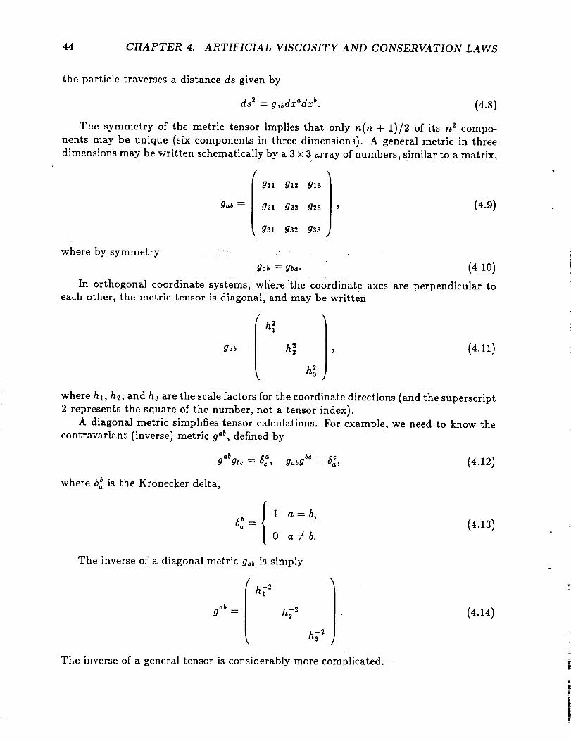
44 CHAPTER 4. ARTIFICIAL VISCOSITY AND CONSERVATION LAWS
the particle traverses a distance ds given by
ds 2 = gabdx"dx b. (4.8)
The symmetry of the metric tensor implies that only n(n + 1)/2 of its n 2 compo-
nents may be unique (six components in three dimension_). A general metric in three
dimensions may be written schematically by a 3 × 3 array of numbers, similar to a matrix,
gn g12 gls )
g "b= g2t g22 g_s , (4.9)
g31 g32 g33
where by symmetry _
=g o. (4.1o)In orthogonai coordinate systems, where :the coordinate axes are perpendicular to
each other, the metric tensor is diagonal, and may be written
gab (4.11)
where hi, h2, and ha are the scale factors for the coordinate directions (and the superscript
2 represents the square of the number, not a tensor index).
A diagonal metric simplifies tensor calculations. For example, we need to know the
contravariant (inverse) metric gab, defined by
gab gb¢ = 6_, gabg bc = _, (4.12)
where _ is the Kronecker delta,
0 a_b.(4.13)
The inverse of a diagonal metric g,_b is simply
hi -2
gab = h_ 2
h_ 2/ (4.14)
The inverse of a general tensor is considerably more complicated.
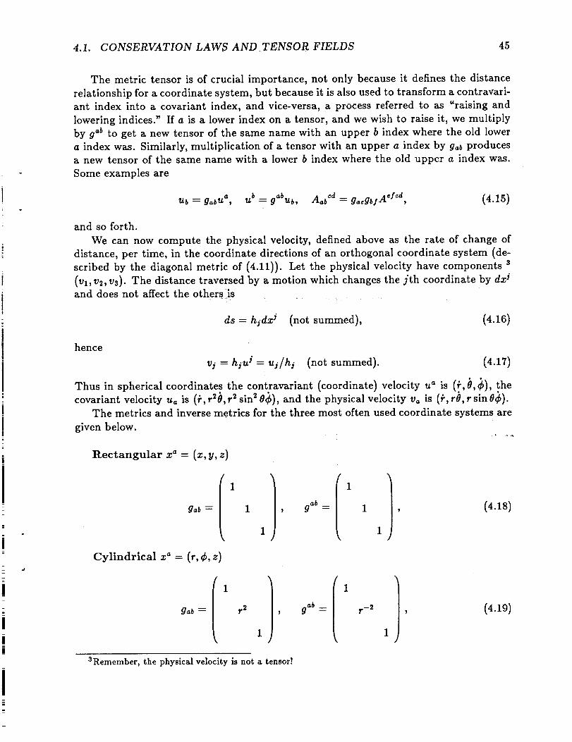
4.1. CONSERVATION LAWS AND .TENSOR FIELDS 45
The metric tensor is of crucial importance, not only because it defines the distance
relationship for a coordinate system, but because it is also used to transform a contravari-
ant index into a covariant index, and vice-versa, a process referred to as "raising and
lowering indices." If a is a lower index on a tensor, and we wish to raise it, we multiply
by gab to get a new tensor of the same name with an upper b index where the old lower
a index was. Similarly, multiplication of a tensor with an upper a index by gab produces
a new tensor of the same name with a lower b index where the old upper a index was.
Some examples are
Ub = gabU a, Ub = gabub, Aab cd = gaegbfA eyed, (4.15)
and so forth.
We can now compute the physical velocity, defined above as the rate of change of
distance, per time, in the coordinate directions of an orthogonal coordinate system (de-
scribed by the diagonal metric of (4.11)). Let the physical velocity have components s
(vl, v2, v3). The distance traversed by a motion which changes the jth coordinate by dx j
and does not affect the others iis
ds = hjdx j (not summed), (4.16)
hence
vj = hju j = uj/hj (not summed). (4.17)
Thus in spherical coordinates the contravariant (coordinate) velocity u a is (._, 0, ¢), the
covariant velocity Ua is (_,r20, r2 sin 2 0¢), and the physical velocity Va iS (_,r0, rsin0¢).
The metrics and inverse metrics for the three most often used coordinate systems are
given below.
Rectangular x a = (z, y, z)
(1/ /1)gab = 1 , gab __-- 1 , (4.18)
1 1
Cylindrical x" = (r, ¢, z)
/ } / }i 1 1
i gab = r 2 , gab = r_ 2 ,
i 1 1
3Remember, the physical velocity is not a tensor!
(4.19)
46 CHAPTER 4. ARTIFICIAL VISCOSITY AND CONSERVATION LAWS
Spherical x a = (r, 0, ¢)
/1 / /1 /gab --= r 2 , gab = r- _ . (4.20)
r 2 sin 2 0 r -2 sin -2 0
4.1.3 Combining Tensors
New tensors may be generated from old tensors in a variety of ways. Two tensors of the
same type may be added to give a third of that type:
Ab_ = Bb_ + ebb. (4.21)
The product of two tensors of rank rn and n is a new tensor of rank m + n,
Aab cd -_ Bab Cod, (4.22)
provided no two indices are the same. If two indices (one up, one down) are the same,
the implied summation produces a new tensor whose rank is two less than the original,as in
R_' = S _ be, (4.23)
Tab¢ : Fade Gbc de. (4.24)
The summation process is often called contraction, and is a frequent occurrence in
tensor calculus. As the number of indices involved increases, the number of terms in
the sum increases rapidly. For example, the contraction of a tensor R_b_d with itself to
produce a scalar R, according to
R = Rabcd Rabcd, (4.25)
has 34 = 81 terms in 3 dimensions. 4
4.1.4 Covariant Differentiation
Another way to generate new tensors is to differentiate old ones. The derivative of a
tensor with respect to a scalar is a tensor of the same type as the first, as in Eq. (4.7)for the coordinate velocity. 5
The derivative of a tensor with respect to a coordinate direction is usually not a
tensor. Such an object is represented either by the usual derivative notation, or by a
subscript comma followed by an index indicating the direction of differentiation, as in
Of OTab c
_x a = f,_, Ox e-= TabC,e. (4.26)
4Such an operation occurs in 4 dimensions in the calculation of tidal forces near black holes, and thecorresponding sum has 256 terms!
5In relativistic calculations, the time coordinate is part of the four dimensional coordinate vector, nota scalar, and a different definition for velocity is used.
4.1. CONSERVATION LAWS AND TENSOR FIELDS 47
I
Note that the gradient (O/Ox °) of a scalar is always a tensor (a covariant vector), while
gradients of tensors of rank one (vectors) or higher are in general not tensors.
One can define a more general derivative operation than the above which does yield
tensor results when applied to a tensor (i.e., which is coordinate invariant). The operator
is known as the covariant derivative and it reduces to the ordinary derivative of (4:26)
when the original tensor is a scalar, or when the coordinate system is rectangular.
The definition of the covariant derivative involves the connection coefficients F abe,
= gadF dbe, (4.27)
1 0g.o 09 o) (4.2s)r b0 = + o d)"
Note that F_ is not itself a tensor, although for computational convenience I have usedthe metric to raise and lower its first index. The connection coefficients for rectangular,
cylindrical, and spherical coordinate systems are given in Appendix A. It is a convenient
fact that the connection coefficients for rectangular coordinates are all zero. Note that
the coefficients are symmetric on the last two indices (£_¢ = £¢_b), due to the symmetry
of the metric.
The covariant derivative of a tensor in coordinate direction a is denoted by the sub-
script ;a. The following are useful examples:
A;a = A,a, (4.29)
I
a a (4.30)B ;b=B ,b+F_ab B_,
" Ba;b= Ba,b- r:bB , (4.31)
t_ab _ab _ ra t-db _ rb _ad (4.32)_-_ ;c = _' ,c 7- Xdc _-_ 7- Xde "J ,
a a d d a (4.33)C b;_ = C b,e + rd_C b- rb_C d,
• '_ _ (4.34)Cab;c _ Cab,c -- raeCdb -- _bcCad.
Covariant derivatives exist for tensors of all ranks, but it will not be necessary to illustrate
any more of the possibilities than given above.
One useful property of the definition of c0variant differentiation is that the covariant
derivative of the metric is always zero:
gab;e = gab;e = O. (4.35)
i Thus the metric commutes with the covariant derivative operator, and we may writeexpressions such as
T ab ' T abd' T abd (4.36)e;e = [,gcd );e : ged ;e.
i Covariant derivatives also obey the usual sum and product rules as ordinary derivatives.

48 CHAPTER 4. ARTIFICIAL VISCOSITY AND CONSERVATION LAWS
The covariant derivative as defined above adds a single covariant (lower) index to a
tensor. We can define a "contravariant derivative" by raising the derivative index withthe metric:
Tab¢ ;e _ gdeTabc;d = (gdeTabc);d. (4.37)
The contraction of a covariant derivative with an index of the original tensor is often
called the covariant divergence. Examples of covariant divergence are Va;s, Tab ;b, and
so forth. While the preceding formulas apply just as well to the divergence as to single
derivatives, there are some special relatk)ns which simplify the divergence calculation.
If we write the metric gab as a matrix, then we can compute its determinant. Let
g _ V/I det(gsb) ]. (4'38)
Then it can be shown that10g 0
Fb_ = g Oxg -- _x _ In g, (4.39)
and the divergence of a vector V s is
1 0
"V._ = g Ox s (gVS). (4.40)
4.2 Fluids as Tensor Fields
Three types of fields are encountered in inviscid fluid dynamics. The density (p), pressure
(p), a,nd total energy density (e) are scalar fields. The coordinate velocity (uS), momen-
tu_ density (rna = pus = pgsbub), mass flux (puS), and total energy flux ([e -+- p]u a)
are vector (first rank tensor) fields. The momentum flux (puSub + p6_) is a second ranktensor. 6
The scalar conservation laws for density and total energy are
Op: O---t+ (PUS);s = O, (4.41)
Oe
. O--t+ [(e + p)ua];s = O. (4.42)
The momentum equations are more complicated. First we define the (symmetrical)
momentum flux tensor [12]
Tsb = puau b + pgsb, (4.43)
or, _quivalently,
The momentum equations are then
Tba = pusu b + p6_. (4.44)
Om a
O---'-i-+ Tab;b = O, (4.45)
eIf it weren't for the momentum flux, we could get by With the simpler formalism of vector calculus,
but such, alas, is not the case.
4.2. FLUIDS AS TENSOR FIELDS 49
Oma
0---7-+ (m.e + =o.The system is not complete without the following auxiliary relations.
velocity magnitude; then
l) 2 _ Ua ua = gabualz b.
For a perfect gas, the pressure is given by the equation of state
p= 1),,
(4.46)
Let v be the
(4.47)
(4.48)
(4.49)
i " so that the individual components of momentum density are not conserved in general,even though the momentum field as a whole is. Note, however, that the rectangular
, components of momentum density are conserved, since in rectangular coordinates g = 1
and Og_'_/Ox a = 0, so that
i aff,,f-_ ma gdx'dx'dx s = 0 (rectangular coordinates) (4.56)
assuming p is constant over the boundary.
The reader who is impatient to see what the complete set of fluid equations looks likei
may turn to Appendix A, where the equations are written out in full for the three most
popular coordinate systems.
1
E = e _pv2_Z
i where e is the thermal energy density.
The above equations are useful for formal analysis, but their numerical solution re-
1 quires writing the equations explicitly in terms of ordinary derivatives. Using the diver-gence relations of the preceding sections gives the more familiar-looklng results:
Op 1 0 ,,+ -_ff-_(gpu ) = 0, (4.50)0---_
3--
i_0e 1 0
0"-'[+ g-_x _[g(e + p)ua] = 0, (4.51)
"i a--It + Y_'" (grnaub) + Ox--'_+ _pu,ud Ox" = O. (4.52)
I The last term in (4.52) is a "centrifugal force term," which arises in non-rectangular
i geometries. "- Integral forms of the conservation laws may be obtained by multiplying each equation
" by the volume element gdxldx2dx s and integrating over the volume desired. If the
velocity goes to zero at the boundary of the volume, we get
, a/f,,/] d'"t P g dx'dx'dx s = O, (4.53)
,if,,/d---t e g dxldx2dx s = 0, (4.54)
and the total mass and energy of the system are constant. The momentum integral is
d f fvf f fvf (Op 10ged'_-_ magdxldx'dxS= - _ q- _pueud---_Xa ) gdxldx'dx 3, (_4.55)
50 CHAPTER 4. ARTIFICIAL VISCOSITY AND CONSERVATION LAWS
4.3 Dissipation for Tensor Fields
Let U be a generalized density (scalar, vector, or tensor) and F = F(U) be a generalizedflux, satisfying the conservation equation
0U
0--/- + div(F) = 0, (4.57)
where diviF ) is the divergence operator defined in the previous sections. Eq. (4.57) isrepresentative of all the fluid equations.
If the relationship F = F(U) is nonlinear, shock waves are likely to arise in the
solution of Eq. (4.57). Even if the flux function is linear, we may still have contactdiscontinuities in the solution,
Therefore the numerical solution to Eq. (4.57) is likely to require the addition of
artificial viscosity, or dissipation, to prevent nonphysical oscillations and nonlinear insta-
bilities in the presence of discontinuities.
The added dissipation must be formulated with care, in such a way as to produce
physically meaningful solutions. One could define many dissipative terms which would
damp oscillations but introduce nonphysical behavior into the solution.
We add dissipation to the numerical solution by replacing Eq. (4.57) with the equation
aU
a--T + div(F) = D, (4.58)
where D is the dissipative term. For the presence of D in Eq. (4.58) to give meaningful
nun/erical solutions to the inviscid Eq. (4.57), we require the following conditions:
1._ D does not contribute as a source term for conserved fields when integrated over
any finite volume, although it may contribute a flux across the boundary of thatvolume;
2. D acts to diffuse (spread out) sharp gradients and damp oscillations;
3. D is written in a general form which is valid in all coordinate systems;
4_ D is isotropic-there are no preferred coordinate directions;
5.. D vanishes as all grid intervals (At, Ax=) go to zero (consistency condition).
The first point requires that D be written as the divergence of some kind of flux. The
second point requires that the flux be a diffusive one, involving derivatives of order no
higher than first. The third point is satisfied automatically if D is written in tensor form.
The fourth point requires that the diffusion coefficient which appears in the flux be a
scalar, not a tensor of nonzero rank. The fifth point requires that D be proportional to
some power of a grid interval, and for the fourth point to be satisfied that grid interval
must be At, and not one of the spatial intervals Ax a.
4.3. DISSIPATION FOR TENSOR FIELDS 51
In Chapter 2 we found that a monotonic (oscillation free) solution for single wave
equations could be obtained by adding to the right side of the equation the term
At / '
Iol az _ However, we now require thatwhich is a diffusive term with diffusion coefficient 2 --_-'
Ax not appear explicitly in the coefficient, so as to preserve isotropy in the multidimen-
sional case where we will have multiple grid intervals Ax a. We write D as a diffusive
term of the form
D = div[_ grad(U)] (4.59)
where _ is a function of position. Eliminating Ax from the above diffusion coefficient in
favor of a, a, and At gives
where a is the Courant number.
systems in a later section.
a 2
=kate, (4.60)
This definition will be extended to multidimensional
4.3.1 Scalar Fields
If U is a scalar field U, the flux F is a vector with components F _, and the conservation
equation with dissipation may be written
OV ;a (4.61)O'---t-+ f';o = (_U);_,
OU 1 O . a" 1 O (gtcU;a) (4.62)"-_ + g-_x_ Cg F ) - g O'-xa
OU 1 O . a- 1 O [ ,_bOU'_
at + g_x _ (gf ) -- g Ox" _gtcg -5-_x_} . (4.63)
4.3.2 Vector Fields
If U is a covariant vector fielJ U_, and the flux F is a tensor F_, the conservation
equation with dissipation is
OU, (K;U: b) (4.64)0----[-+ F"b;b = ;b"
Working out the covariant derivatives on the right and making use of relation (4.39) gives
ouo 1 o (ouo r2 vd -r:0 "O----t- + Fab;b -- g Ox ¢ ggbCr_ _, OX b
7Similar results apply to contravariant vector fields, but the momentum density is most conveniently
expressed in terms of covariant fields, so we consider only the covariant case here.
52 CHAPTER 4. ARTIFICIAL VISCOSITY AND CONSERVATION LAWS
Unfortunately we cannot eliminate the connection coefficients I'_c in favor of simpler
expressions, as we did for the scalar equation. The presence of the connection coefficients
produces the inhomogeneous term on the right, which implies that the components of
Ua are not conserved in general, except when rectangular coordinates are chosen. In
rectangular geometry all F_c = 0, and we see that the rectangular components of Ua are
conserved. The dissipative operator conserves precisely those components of the field
as does the original momentum equation! That the same conservation properties hold
in both cases is not an accident, but is a basic property of the geometry of coordinatesystems.
4.4 More on the Dissipation Coefficient
The fluid equations with dissipation are given in full in Appendix A, and will not be
repeated here. Now we will look at the definition of the dissipation coefficient _ in moredetail.
As shown in Chapter 2, the choice
a2=kate, ,, = a(u) , (4.86)
reproduces the monotone first order scheme of (2.37) when k = 1/2, but does this
definition (and its generalization to higher dimensions) have the conservation, isotropyand coordinate invariance properties we seek?
The answer is a qualified yes. Isotropy can always be maintained by defining J¢
uniquely at each grid point, so that dissipation occurs at the same "rate" in all coordinate
directions. Conservation is guaranteed by the divergence form of the dissipative term,
so only coordinate invariance needs to be investigated further.
The definition of _ given above is not coordinate invariant, nor should it be. The
dissipation depends on the choice of grid, as it must in order to satisfy the consistencycondition, and will change as the grid parameters change. Thus _: is not invariant under
grid changes in any given geometry. Moreover , coordinate rotations in multidimensional
problems will alter the characteristic velocity components, changing a and a, and hence
_:. Thus _ is not invariant under coordinate rotations, and is not a scalar.
What happens, then, when we do perform a coordinate transformation on some phys-
ical problem and solve the problem numerically in both coordinate systems? Will the
two solutions agree? They will, provided both have adequate resolution. By "agree"
I do not mean agree exactly (an obvious impossibility, since the two solutions will not
even be computed at the same grid points), but the solutions should agree to within 1%
or so, except possibly at discontinuities. The diffusion coefficient i¢ adjusts automati-
cally to changes in the grid and coordinate system so as to apply the correct amount ofdissipation needed in each case.
Although strict coordinate invariance is neither necessary nor desirable, strict isotropy
is both. If _ is computed differently in the diffusive terms for different coordinate di-
rections, then it is really "simulating" a tensor _. For any given problem the results
4.5. DISSIPATION IN ONE DIMENSION 53
|
|
i|
i
may appear reasonable. However, to reproduce those results in a new coordinate systema #
,' A,'Ab • - and using t%, in the new system. Ifwould require transforming t;_ into _;v = ", "-v%,
the transformation is not performed, the two solutions will in general not agree. If the_Wtransformation is performed, the new _;v is likely to contain off diagonal elements and
be an explicit function of the transformed coordinates, even though the original _;_ was
a diagonal tensor with constant elements.
Tensor diffusion coefficients may have a role to play in the real world (such as diffusion
and heat conduction in anisotropic materials), but they are of no use in artificial viscosity.:.
%
4.5 Dissipation in One Dimension .
This section illustrates one method for raising the order of the dissipative terms to provide
a globally second order accurate solution, for single equations and the one dimensional
fluid equations. To get a second order scheme, simply multiply the definition of (4.66)
by a function v(U) which is also first order,
a 2
= k_t_,, (4.67)ivl
where v _ 1 in oscillatory regions and near discontinuities, and is a first order quantity
otherwise. One definition which has proved quite useful is
Iu,+,- 2u, + u,-,I (4.6s)" = Iu,+, - u,I + Iu, - u,-,l'
where U_ is the numerical solution at grid point x_. ._
In summary, we make a finite difference approximation to the dissipative equation
0: 0" : -_+,_ _ k a_]' :=/('4'
(4.69)
(4.70)
as in Chapter 2. The semi-discrete approximation is
1dtZ, -16c_)/,+ [_,+,/_(u,+,- u,) - _,_,/_(u, - v,__)],dt -- Ax _ _
using the definition (4.67) for _;, where the wave velocity a = df/du, and the constant
k is constrained by k]a] < 0.6963, for the integration schemes (2.30) and (2.31). (The
choice k = 0.3 is often effective.) Note that the quantities f, to, a, and a = aAt/Ax are
local functions of U and will generally vary from place to place. "'
Now consider the more difficult problem of fluid dynamics in one dimension, chopsing
spherical geometry for the coordinates. Retaining only the radial terms from Eqs. (A.43)-
(A.45) gives
i:3p 1____ l O [, i)p) (_I.71)_+;z ("'"':)- #_ V" '_ '
54 CHAPTER 4. ARTIFICIAL VISCOSITY AND CONSERVATION LAWS
where
0--;+ [r_(e+ P)_'] = r' Or r_ ' (4.72)
am, 1 a _ , ap 1 a _r2 arn,._ 2aT + _(r m,_ ) + ar - # _r _ ar / ;Z_m'' (4.73)
u':m,./p, (4.74)
p = ('_- 1) (e 1 ,2) (e 1 ,_m,,u ) (4.75)-- _pu = ('_-- 1) --
and _ is a constant (5/3 for a monatomic gas). Here u" is the coordinate velocity, whichhappens to be the same as the physical velocity v, in this case.
The semi-discrete approximation to these equations is
dpi 1Adt - r_ r6(rm}(r_piu_')
21 [ri+l/21£i+l/2(Pi+l Pi)- 2
-_-_r_ Ar 2 -- ri-1/2t_i-1/2(Pi - Pi-,)] , (4.763
dei 1 8(,.,.,)d-T -- r_Ar " [r_(e, +pi)u_]
21 [r,+ln_,+ln(_;+l _d--_-_r_Ar 2 - ri-l/2_i-,/2Cei -- ei-1)] , (4.77)
dmr i
dt
l [ri2+l/_,i+l/2(rn, -mri)-r 2"f-r_Ar-"'-'_ i+, i-1/2tCi-1/2(mri- m,i-1)] (4.78)
2r2 Eimri.
i
To compute the diffusion coefficients we need to define an effective wave speed a. In
the case of a single equation, a was just the local value of df/du. In the current problem
we have three equations, and there are three characteristic velocities (as will be shown in
Chapter 5). The three characteristic velocities are u'-c, u', and u'+ c, where c : _-p/pis the speed of sound. The amount of dissipation needed is governed by the most rapidly
changing wave. Hence we define the quantity c, to be the magnitude of the greatest wavevelocity in the r direction,
e,, = lu:l+ e,, (4.79)
Ate" (4.80)ai : Ar'
and set
ai = Cr i.
Then the dissipation coefficient is given by
a,_ 1_, : kAtie, iv,, /_i-t-1/2 : _(/_i-_ /_i+1),
(4.81)
(4.82)
4.6. DISSIPATION IN TWO AND THREE DIMENSIONS 55
where v_ may be made a function of any solution component (p, m, e, or some combina-
tion). The choice v = v(p) has been found to be effective, so we define
]p,+l - 2p, + p,-l[ (4.83)
_' = Ip,+l- p,l + Lp,- p,-II"
Note that the equations are undefined at r = 0, because of the coordinate singularity.
The time derivatives become infinite at r = 0 unless u'(r = 0,t) = 0, in which case
L'Hopital's rule gives
(o )t (4.)ap a _arra-; +3 (P"') = 3b-;r ,=o'
0, 0 (4,,)a---t+ 3 [(e + p)u'] = 3_r \ Or] ,=o'
rn,. = 01 (4.86)r .._.0"
We know from the condition of spherical symmetry that p, e, and p are symmetric
functions of r, while m, and u r are antisymmetric, and can use these symmetry conditions
to evaluate the finite difference approximations at and near r = 0.
4.6 Dissipation in Two and Three Dimensions
The simplest two dimensional problem is the single conservation law of Eqs. (2.45)-(2.46),
to which we add dissipation as follows:
a-/+_-_x+a_- axk a=)+_\ oH'
The x direction characteristic velocity is a = df/du, and the y direction velocity is
b = dg/du.The semi-discrete approximation to (4.68) is
dU_jdt _T, z J'3
1 iCU,+, U,i) - _,-,/2 j(U,i - U,-1 i)]+_=_['q+l/= i -1
+-E_y_i_,_+,/=(u,_+,- u,i) - _,__l/2(u,j - u,i-,)].
(4.88)
The local Courant number is
Ay]
Now select the dissipation on the basis of the maximum velocity component,
c,¢ = max(la,jl, Ib,,I), (4.9o)
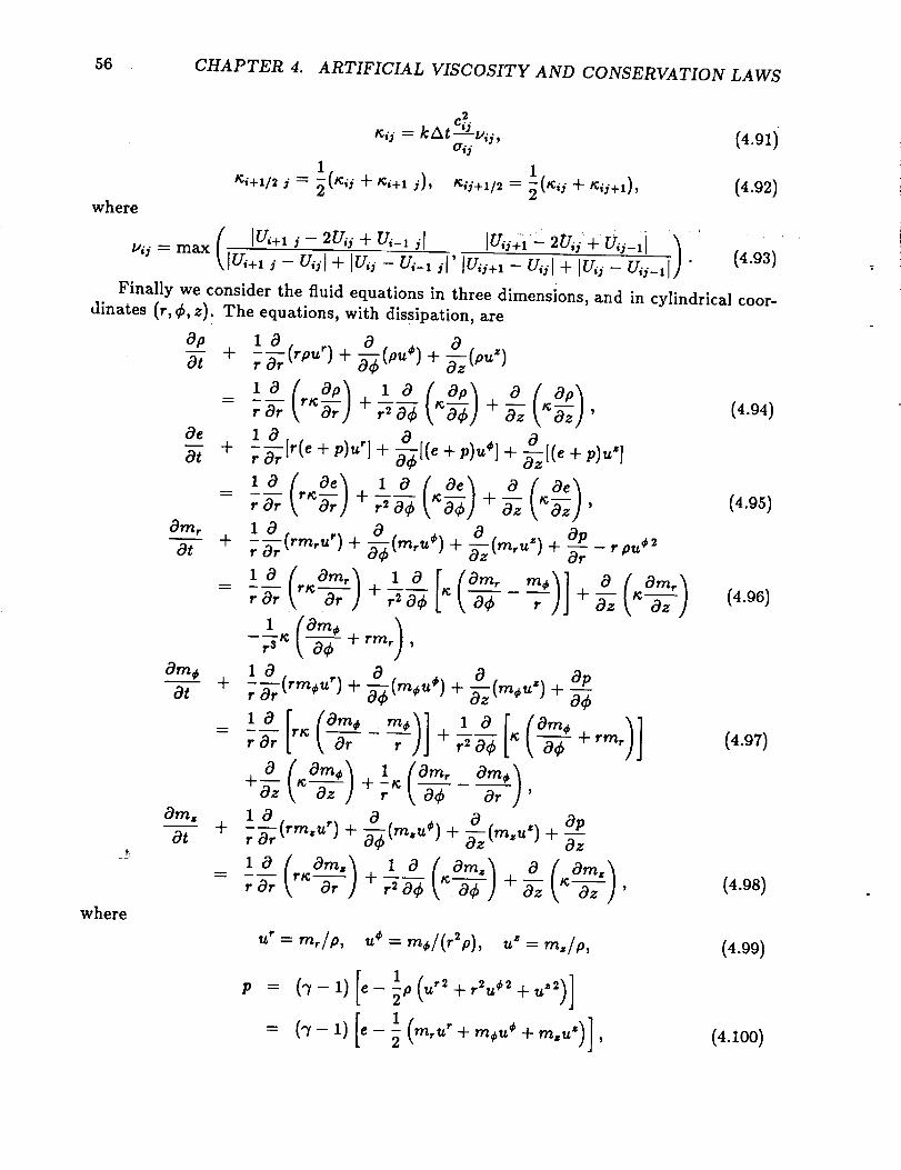
56 CHAPTER 4. ARTIFICIAL VISCOSITY AND CONSERVATION LAWS
c?.
_ij = kAt -*_ viy, (4.91)aii
1 1
_,+,1,i = _(,_,i+ _,+, D, _,J+,l, = _(_,_+ _,;+,), (4.92)where
,IUi+, j-- 2Uij + Ui-z j[ IUii+, ± 2U, i + Vii',] _ ' (4.93)_'ii= max Iui+,s - uiil + Iu,¢- u,_, iJ' Juii+,- u,¢J+ Iuii - u,j-,I]
Finally we consider the fluid equations in three dimensions, and in cylindrical coor-dinates (r, ¢, z). The equations, with dissipation, are
Op 1 O r O_ Oo-7 + 7_ (rp=) + (P=+)+ _(p= )
_ 1 0 rlCor-r +---- m + m (4.94)r Or r2 0¢ _z '
Oe 1___ _ O0-7 4- - [r(e 4- p)u'] 4- [(e 4- p)u _] 4- -_z[(e 4- p)u =]r
(o,) lO(b_ 1 O r_orr 4----- _ 4- (4.95)r or r_0¢ _z t Oz]'
at- + ('_.") + (m.,+) + (,,.=') + _ - rp,,+,
r-_ _ 4- rrVir ,
at 4- (rm@u') 4- (m@u +) 4- (re+u*) 4- a--¢
,o[ to-, ,o[ro., )]-- r Or r_ t Or 4- r--_a--¢ _ t De 4- rm, (4.97)
+_ '_ az )+r toe _)'
Ore= 1 0 , _ O = Opat + -r =_r (rm=u) 4- (re'u+) 4- -_z (m'u) 4- Oz
-- r Or r_ 4- r-lO-¢ _ 4- azz t_C-_z ) ' (4.98)
where
P
"'= "',lp, "" = ""+l("'p), "" = "".:lp,
= (,-l)[e-2P(u'i-l-riu+'4-u=,)]
-- ("'/- 1) [e
(4.99)
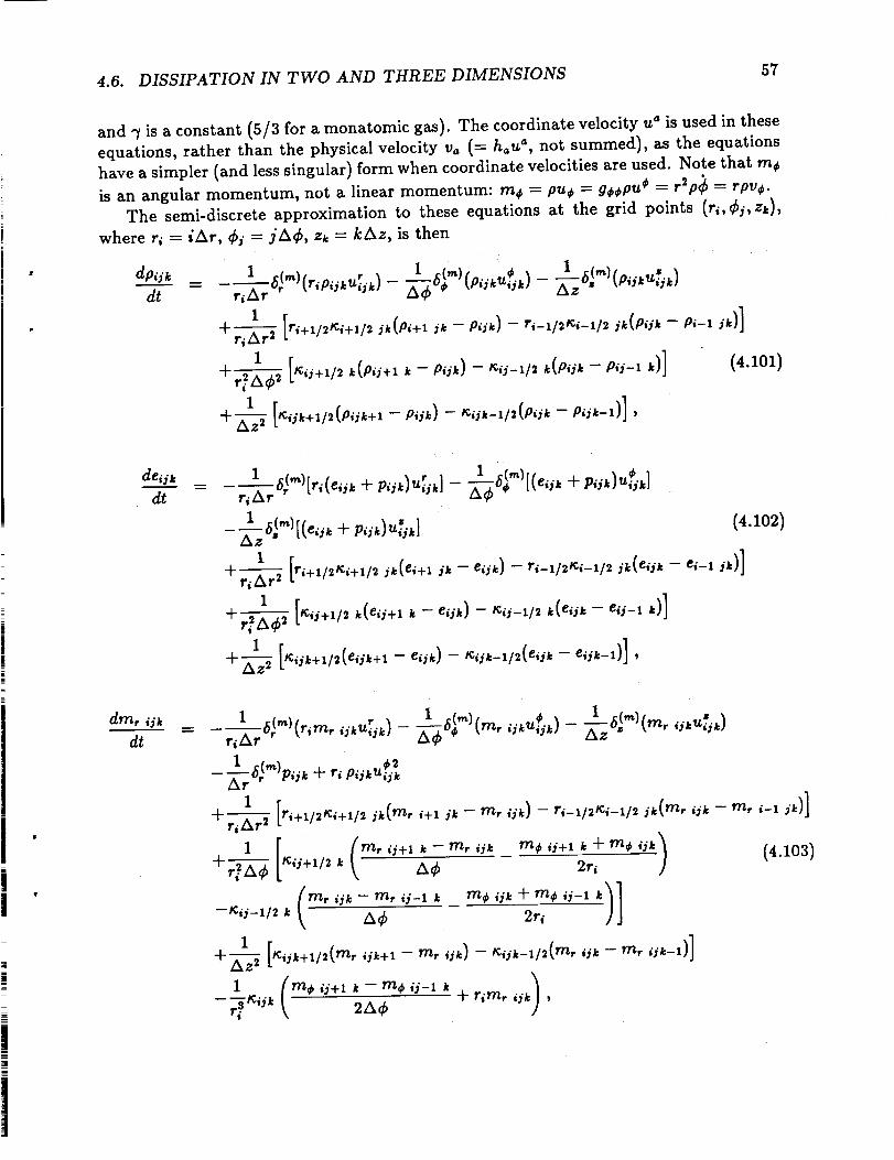
4.6. DISSIPATION IN TWO AND THREE DIMENSIONS 57
and ff is a constant (5/3 for a monatomic gas). The coordinate velocity u" is used in these
equations, rather than the physical velocity v, (-- hau _, not summed), as the equations
have a simpler (and less singular) form when coordinate velocities are used. Note that me
is an angular momentum, not a linear momentum: rn_ = pu÷ = g_pu _ = r2p¢ = rpv_.
The semi-discrete approximation to these equations at the grid points (r_,¢j,zk),
where r_ = iAr, Cj = jag?, zk = kAz, is then
dt
1 [r,+,/.,_,+,/__(.,+,_.- p,_)- .,-,/.,_,-,/.J_(.,_.- p,-,;_)]
1 [_,_+,/,,C,,_+,,- p,_,)- _,i-,/,,(.,_,- .,_-,,)] (4.101)
+_z_z2
deijk
dt
1 z 6(,,_)[(eij, + pok)ui_, ] (4.102)
+,,-7_,'
+-_-_z_
i I!
dfflr ijk
dt
(4.103)
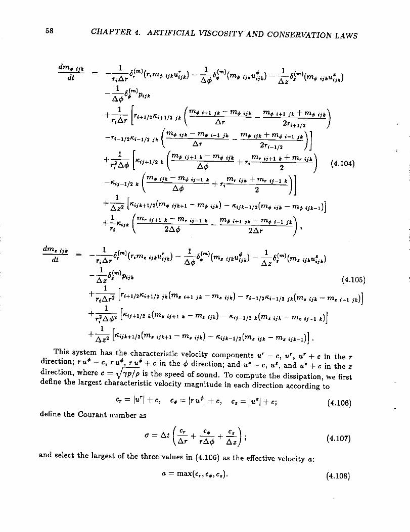
58 CHAPTER 4. ARTIFICIAL VISCOSITY AND CONSERVATION LAWS
dt ';* ,*) X_ s _ s sriAr r t S ijkUZj.k)
jk ms i+i _k -- rns O'k _ rns i+1 yk + m s ijk_ar 2ri+1/2
1 6(,_)_."a¢ s t',jk
1 [ri+ll2tCi+ll2
[
(mS iik--rn s i-1 yk ms iik-_-rnsi-1 jk)l--ri-x/21¢i-1/2 J_ \ Ar -- 2ri-1/2 /J
"_r2-_ I_iy+l/2 k A_ 4- ri 2
--'¢'ii-1/2 k \ _; + ri 2/l
1 [gij,+t/2(rn s rns iik) giyk-1/2(rns ,P, - rns ii*-l)]+ _ iik+l - --
ri _,jk 2A¢ 2Ar '
(4.104)
drn. ijkm Ur
d t ri a r
1 6C,,,)pi .kaz" ' (4.105)
1
+,,-Z_,,["'+'"+" _(r_.,+t_ - _. ,_,)- _,_,.,_,_,/,_(m.., - ,.. ,_,;,)]
+,-ta_--_l[,,,+,/, ,(m.,+, . - r_.._)- _,_,, _(m.,_,- m.,____)]
+X-_z' '_+' - ,i*)- '_,_-,,('_.,, - m.,__,)].This system has the characteristic velocity components u r - c, u', u" + c in the r
direction; ru¢ - c, ru s, ru s + c in the ¢ direction; and u _ - c, u _, and u = + c in the z
direction, where c = V/_ is the speed of sound. To compute the dissipation, we first
define the largest characteristic velocity magnitude in each direction according to
c,.= I""l+c, cs=l,-,,sl+c, c,=lu=l+c; (4.106)
define the Courant number as
Cr C s C z )o=at _+-h-_+_ ;
and select the largest of the three values in (4.106) as the effective velocity a:
a = max(c,, cs, c,).
(4.1o7)
(4.108)

4.7. COORDINATE SINGULARITIES 59
The dissipation coefficient is then
a.2a_i_ = kAt_--itv_i k' (4.109)
where uii_ is taken to be
/ ]Pi+I jk- 2pijk _- Pi-1 _kl Ipi_+lk -- 2Piik + Plj-1 k[ ['
(4.110)Ip,j_+l- p,_,l+ lp,_ - p,i_-lb"
where p is the pressure. As usual, the dissipation coefficients at the half points are given
by
1 1 1
_,+1/2j_ = _(_,_ + _,+1_), ,_,i+1/2, = _(,_,i_+ '_,_+1_), _,_,+1/2= _(_i_ + '_,_,+1).(4.111)
4.7 Coordinate Singularities
The fluid equations given above for cylindrical coordinates contain a coordinate singu-
larity at r = 0. In the one dimensional spherical case we dealt with the singularity at
r = 0 by requiring that the divergence term in each equation be finite, which allowed us
to use L'Hopital's rule to get a non-singular limiting form at the origin. We generally
cannot require that each divergence term in an equation be finite at a singularity when
dealing with two or three dimensional problems, as it is only necessary that the sum
of all divergence terms be finite. (This problem becomes particularly acute in spherical
coordinates, which is singular at r = 0 for all 8 values, and at 8 = 0, 0 = r for all r
values.) It is quite possible that any given term may tend to infinity as at the singularity,
even though the sum of all such terms in the equation is finite.
The completely general three dimensional problem in non-rectangular coordinates
is probably best handled by reverting to the rectangular coordinate definition for the
divergence at the singular points, if individual terms are known to become infinite. If
on the other hand particular symmetries of the problem dictate that individual terms
remain finite at singularities, then L'Hopital's rule may be used to obtain a limiting form
for the equations.
4.8 Dissipation for General Hyperbolic Problems
i So far we have looked only at the fluid dynamics equations. However, the formalism
used above may be stated in very general terms for any first order system of hyperbolic
4 conservation laws, in any number of spatial dimensions. In this section I will describe
how to construct dissipative terms for an arbitrary system in three spatial dimensions,
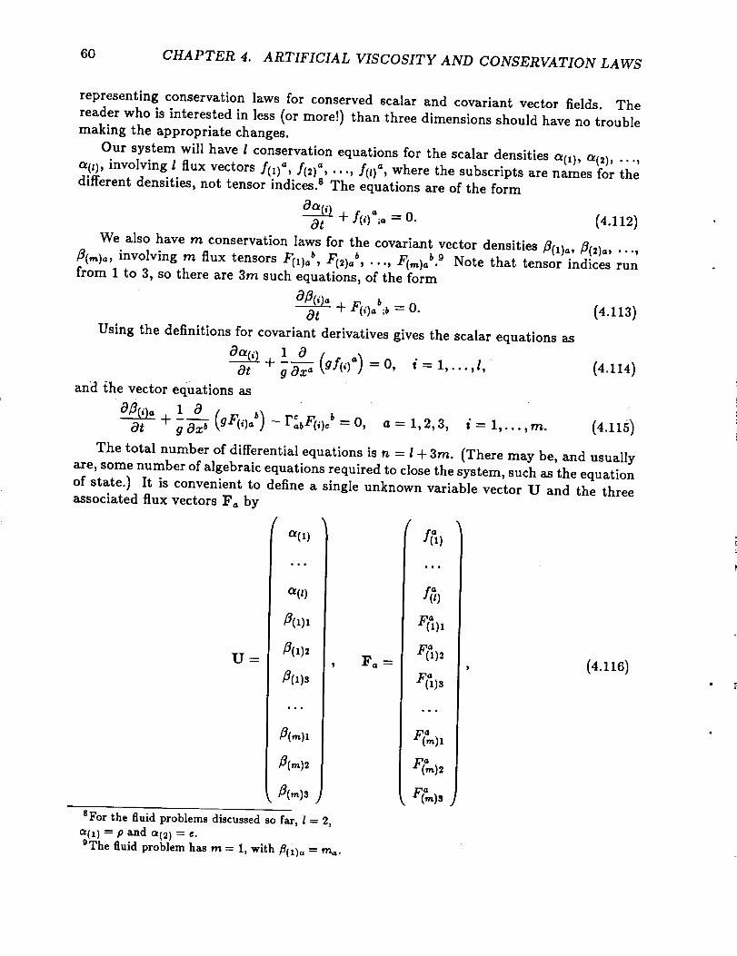
60 CHAPTER 4. ARTIFICIAL VISCOSITY AND CONSERVATION LAWS
representing conservation laws for conserved scalar and covariant vector fields. The
reader who is interested in less (or more!) than three dimensions should have no troublemaking the appropriate changes.
Our system will have I conservation equations for the scalar densities a0) , a(2), ...,off_), involving I flux vectors ]'(i) a, f(2) _, ..., f(0a, where the subscripts are names for the
different densities, not tensor indices, s The equations are of the form
+ =0. (4.112)Ot
We also have rn conservation laws for the covariant vector densities _(1),, f_(2)o, ...,D(,_),, involving m flux tensors F(1), b, F(2), b, ..., F(,_)ab) Note that tensor indices run
from 1 to 3, so there are 3rn such equations, of the form
+ F(,),b;a = 0. (4.113)0t
Using the definitions for covariant derivatives gives the scalar equations as
+ 1 0._0 _f(,),) = O, i= 1,. ,l, (4.114)Ot g Ox = ""
and the vector equations as
r,_F(,)o -0, a = 1,2,3, i= 1,...,m. (4.115)
The total number of differential equations is n = l + 3rn. (There may be, and usually
are, some number of algebraic equations required to close the system, such as the equation
of state.) It is convenient to define a single unknown variable vector U and the threeassociated flux vectors F_ by
0/(1)
a(0
_(1)1
U = _(1)2
8(1)3
_(,,)2
_(,,)3
SForthe fluidproblemsdiscussedso fax,I= 2,
_(1) = P and a(2) = e.The fluid problem has m = 1, with fl(1)a = m_.
Fea
( I(%
..a
Fi_)l
F(_)2
o..
F(2)1
Fi2)
Fi )s
(4.116)
4.8. DISSIPATION FOR GENERAL HYPERBOLIC PROBLEMS 61
so that the complete set of conservation laws may be written
OU OF1 aF2 + aFs (4.117)a---T + _-x-i-xl+ -a-_x_ a--_xa+D=0 ,
where D is a vector of inhomogeneous terms. (By vector in this instance I mean any set
of variables in the sense of linear algebra, not a tensor. The objects U, Fa, and D do
not satisfy tensor coordinate transformations.)
The equations may also be written
aU OU + OU OU (4.118)O---T + A_x-_xl B_x2 + C_x3 +D = 0,
where A, B, and C are the n x n Jacobian coefficient matrices with components
OF1 _ OF2 _ aFs _ (4.119)A_ i- au i, Bii- au i, c_i=-au i
Now let the eigenvalues of A, B, and C be _,/_, and rh, i 1,..., n. These eigenval-
ues are the characteristic velocity components for the associated coordinate directions:
),_ for the x 1 direction,/z_ for the x _ direction, and rh for the x s direction. The extreme
values arecl = maxl_il, c_ = max I#,1, _. -- maxl,7,1, (4.120)
and the largest of these is, _ " a = ni_x(c,,c2,cs). (4.121)
The dissipation coefficient is therefore
a 2
t¢ = kAt--_,G
(4.122)
where the Courant number is
( c I c 2 ' c3 ),, = :,t h--_=.+ _-_ + h--_. •
The quantity v at grid point (x_,x_.,x_) is then
l//jk ----
(4.123)
( If,+. _ - 2f,_ + f,'. _1 If,_+._- 2f,_ + f,_-__lmax_,lf,+,;_- f,_l + ]f,J_- f'-' ikl' I/,i+l _- f,;,.I+ If,i_ -/',_-1 ,.1'
If, i*+1 - 2fok + f, ik-II '_ (4.124)
If, i*+1 - f,i_l + Ifo'_ - f, ik-_l] '
where f is any scalar variable which reliably indicates the presence of discontinuities and
oscillations, such as pressure in the fluid case.
The equations with dissipation are then
1 (9 1 a ( Oa(0 _ (4.125)aa(_) + ___ (gf(,)_) _ g_g_bat g ax = g ax = Oxb )
62 CHAPTER 4. ARTIFICIAL VISCOSITY AND CONSERVATION LAWS
for the scalar fields, and
g cox c g_gb¢ _ d _ tac_g_ b¢ (O_(i)e\ \ azb
for the vector fields, as in Eqs. (4.63) and (4.65).
form is handled as in the previous sections.
(4.126)
The approximation to semi-discrete
4.9 Conservation Properties of Finite Difference Equa-tions
The fluid equations may be written in a variety of forms, such as the conservative forms
described in this chapter, and the characteristic and primitive forms given in Chapter
5. Finite difference approximations may be made to the equations in any form, with
the same formal accuracy, yet all approximations in this text have been made to the
conservative forms. The reader may wonder if there is an advantage to be had in using
the conservative form in numerical work. The answer is yes.
First of all, the artificial viscosity terms require the conservative equations for their
definition. However, once the terms are defined, one could write the equations in an-
other form, so the necessity for artificial viscosity does not require that the numerical
approximations be in conservative form, though they are more simply written in thatform.
More important is the notion of numerical conservation laws. The numerical ap-proximation to the conservative equations possesses an exact conservation law which is
analogous to the original conservation law embodied by the differential equations, and it
is for this reason that the conservative form is preferred in numerical work.
A field u is said to be conserved if it satisfies the equation
0u 1 a
+ g --_xi(gfi) = O,o-T (4.127)
where f_ is the flux of u in the ith coordinate direction. The conservation property is
seen most clearly by integrating Eq. (4.127) over the volume a 1 < x 1 < b t, a 2 g x 2 < b2,a 3 < x 3 < b3: - _
1 0 i//vf gdx'dx'dx'[_t +g-_x_(gf) ] =0, (4.128)
d -b_ b'
f f. f -:.:'].,(,:').,.x',.'b I b 2 b2 %1 bs
(4.129)
4.9. CONSERVATION PROPERTIES OF FINITE DIFFERENCE EQUATIONS 63
The rate of change of the volume integral of u is given by the integral of the fluxes over
the surface bounding that volume.
A properly chosen numerical approximation to Eq. (4.127) retains an analogous con-
servation property [13]. If the semi-discrete approximation is written as
2 21 -- F,1-1/2 jk 1 Fii+l/2 k - Fiy-t/2 k1 Fi+l/2 jk
dUiik + +dt giik AxI giik Ax2
3 3- F, k-i/21 f;sk+,l, (4.130)+ = 0,
giik Ax3
where F l = gfl, then its summation over the volume elements giikAxlAx_AxS gives
d S;,K I,K-- (F;+,/2 ik- F:/, i_)AxiAx sdt _ Uiik giik Axl Ax2 AxS = -- _ 1
i,j,k= l j,k= l
I,K I,J
_ - (F_iK+I/22 2(Fu+l/2 k Fi,/2 k)AxlAx s _ s _ F_.l/2)Ax,Ax n.i,k=l i,j=l
(4.131)
The interior fluxes cancel out of the sums, leaving only the sums of normal fluxes
over the boundary surface. The numerical scheme of (4.130) yields an exact numerical
conservation law. A numerical approximation to a nonconservative equation does not
produce a conserved numerical solution.
Eq. (4.130) makes use of finite difference approximations of the form
OF _ F_+l/1 - Fi-V2 (4.132)Ox Ax '
which involve mid-point fluxes F_+I/-., rather than grid point fluxes F_. The dissipative
terms naturally have mid-point fluxes, since the dissipative flux is F = gt¢ c3u/Ox, for
which Ui+t - Ui (4.133)Fi+I/2 = gi+l/2tCi+l/2 Ax
+ • :
to second order in Az. The convective terms have grid point fluxes F+ g+fi, however,
from which the mid-point fluxes F++I/+ must be constructed for the proof above to hold.
The choice
1 (Fi+l + Fi) (4.134)
recovers the familiar second order result, while
= +F,)- + (4.135)
recovers the fourth order result. Zalesak [14] gives flux expressions up through eighth
order.
Note that it is not necessary to compute F_+l/1 explicitly, as given above, to ensure
numerical conservation. The finite difference formulas previously used are properly con-
servative, as demonstrated by the existence of mid-point fluxes such as (4.133), (4.134),
and (4.135), along with the numerical conservation law (4.131).
64 CHAPTER 4. ARTIFICIAL VISCOSITY AND CONSERVATION LAWS
For example, consider the single equation
0. 10 10 ¢4.136/0-7+ _ (gf) = _o-_ _ o_/ '
where _¢ is the artificial dissipation coefficient. The standard semi-discrete approximation,using a fourth order formula for the convective flux, is
dUd 1 1
dt -- g, 12Ax[8(g,+lf,+l - g,-lf,-1) - (g,+2f,+2 - gi-2fi-2)]
1 1
+-h-_ [_,+1/2W,+1- v,) - _,_l/,(u, - V,_l)],g_
v
which is exactly equivalent to
dud F/+l[2 - F/_l/2
dt - ZXx ' (4.138)
where
7 1
F/+l/2 : "_(gi÷lfi-t-1 Jr gifi) - -_(gi+2fi+2 _- _i-lfi-1) -- _i+1/2
and is therefore numerically conservative.
Vi+ 1 - V i
(4.139)
4.10 Test Problems
We now have at our disposal all the tools needed to obtain the numerical solution of
some typical fluid dynamics problems. For the sake of simplicity, we consider only one
dimensional problems for which the boundary values may be held constant with time,
postponing the discussion of nontrivial boundary conditions until Chapter 5. Both rect-
angular and spherical geometries will be considered, with spatial coordinates x and r,respectively.
These one dimensional test problems are evaluated on a grid of unit length, divided
into 100 subintervals (I = 100, Ax = Ar = 0.01). The value of "7in the equation of state
is 5/3 throughout. The figures show the analytical solutions (solid lines) and numerical
solutions (dots) for the density p, the pressure p, the momentum density rn, and the
velocity v, at a time t. The Courant number a,
czAt
a= Ax' (4.140)
is set to 1 throughout, where c= -- max(Ivz] + c) over the grid (and similarly for c,).
The first example is the shock tube problem, frequently used as a test for hydrody-
namical codes (as in Sod [24]), and whose solution is given by Thompson [25]. At time
t = 0 the system consists of two spatially constant, stationary states, adjoining at x - 0.
The left state (x < 0) has p = p = 1, while the right state has p = 0.125, p = 0.1.
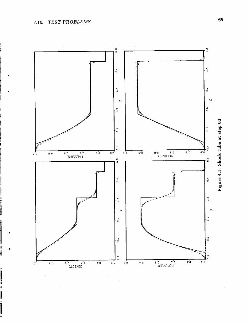
4.10. TEST PROBLEMS 65
0"I
olo
g"o 9'b ,"o
ao o°_o
O' I 8 "*0 9 "0 I_"0 _ "0
IIISN]O
o
o
90'0
to
6
r_
o
X
c3
r_
i
_r
ot
0"0 S'O
0"1 8"0 _'0
to
-o
9"0 _'0
IIIO073A
"o
c_
o
o
r_
-6l
0"0
o
o
o o °
f°°
I o
o
o °°
_"0 _"o _'b _"o 0'0WFIIN3WOW
o
"o
o
o
r_
"ol
Z
o
e_
,.o
0
,q
p_

66 CHAPTER 4. ARTIFICIAL VISCOSITY AND CONSERVATION LAWS
As time progresses, a rarefaction wave forms and moves to the left, while the contact
discontinuity and a shock wave move to the right.
Figure 4.1 shows the solution at time step 60, t = 0.265, with k = 0.3, just beforeany waves reach the boundaries.
The shock wave is located at x = 0.5 and is resolved in _ 3 grid intervals. Small
oscillations occur around the shock. These oscillations could be eliminated by increasing
k, at the expense of spreading out the shock (and other features in the solution). The
contact discontinuity at x = 0.23 is spread out over _ 10 grid intervals. Unlike shock
waves, which keep a constant width, contact discontinuities in the numerical solution
widen steadily with time. The nonlinear nature of the shock wave produces a tendency
to steepen which is countered by the artificial viscosity, so the shock width remains
constant. However, the contact discontinuity is a discontinuity in a linear wave, which
has no steepening tendencies, and therefore spreads monotonically with time as it is
diffused by the artificial viscosity.
A general technique for obtaining sharply resolved contact discontinuities has yet to
be formulated, and it is beyond the scope of this text to describe any of the numerous
experimental methods which have been developed. As a first attempt, one may attempt
to detect the presence of such a discontinuity and decrease the artificial viscosity there
to reduce the spreading rate. However, some viscosity is needed to prevent oscillations
near the contact discontinuity, so the spreading cannot be eliminated by this technique,although it can be slowed. It should also be mentioned that such discontinuities will
spread even in the absence of artificial viscosity, as well as producing oscillations.
The next problem considered is the Sedov solution for a spherically symmetric explo-
sion, described by Landau and Lifshitz [12]. (N.B. Eq. (99.10) of the reference should
have v5 = 2/('7 - 2).) An amount of energy E is deposited at the origin at time t = 0.
The resultant explosion produces a self similar solution bounded by an outgoing spherical
shock wave. The density and pressure curves are sharply peaked at the shock, falling
off rapidly for decreasing r. The density goes to zero at the origin, while the pressure
flattens out and becomes constant with r away from the shock. The velocity is linear
near the origin, but steepens somewhat near the shock. The similarity solution is valid
as long as the shock is very strong, so that the density jump across the shock achievesits maximum value.
The numerical solution is produced by distributing an amount of energy E = 1 over
the innermost five grid intervals, in the form of thermal energy. Let the sum of the
volume elements for the first five points be
5
vol ----47tAr _ r_, (4.141)i=0
then the initial pressure is
P, = ('7- 1)E/vol, (4.142)
for i = 0,...,5. For i > 5, Pi = 10 -6. We also have p = 1 and u = 0 everywhere.
The resultant numerical solution is shown in Figure 4.2 at step 365, t = 0.614, and withk = 0.35.

4.10. TEST PROBLEMS 67
68 CHAPTER 4. ARTIFICIAL VISCOSITY AND CONSERVATION LAWS
The shock wave is very strong, and is resolved in two grid intervals. Once again
a small amount of ringing is observed near the shock, which could be eliminated by
increasing k at the expense of spreading out the shock further. The post-shock density
should peak exactly at a value of 4 for this problem; the numerical post-shock density
is _ 3.25, which is low by _ 20%. The density profile behind the shock is so sharply
peaked that the numerical solution cannot change quickly enough to achieve the correct
density peak. Increasing the resolution of the calculation by increasing the number of
grid points would reduce the error in the peak height. However, the correct shock velocity
is achieved even though the exact post-shock solution is not attained.
The exact solution to the spherical blast wave has the density going to zero at the
origin, while the pressure remains finite and the temperature goes to infinity. The numer-
ical solution cannot reproduce this singular behavior at the origin. Instead the numerical
solution has a very small but nonzero density in the center, and a high but finite tem-
perature. The pressure near the center is accurately represented. Note that the sound
speed is therefore very large at the center, and is Win fact the largest velocity present in
the calculation. The allowed time step is therefore determined by the speed of sound atthe center, and not by the post-shock velocity, which is much smaller.
4.11. EXERCISES 69
i
4.11 Exercises
1. Let x = = (x,y,z) be rectangular coordinates, and let x =' = (r, 0,¢) be spherical
coordinates. Using the relationships of Eqs. (4.6), compute the transformations A_,
and A_'.
2. Using the results of problem 1, write down the coordinate velocities u = = (5, I), _)
in terms of u='= (_,0,¢), and vice versa. Do the results match what you obtain
by taking the time derivatives of Eqs. (4.6)?
3. Let x a = (x, y, z) be rectangular coordinates, and let x °' = (x', y', z') be a different
rectangular coordinate system. The z and z' axes are the same, while the angle fromthe x axis to the x e axis is 0. Compute the transformations A_, and Aa'. Use these
transformations to express the velocity x_ = (_,_,_) in terms of x _' = (x',ye, zi),
and vice versal Are the results _vhat you expect?
4. Verify that the metric g_ and its inverse g_ satisfy relationship (4.12), using metrics
(4.11) and (4.14).
5. Compute the connection coefficients F_c for cylindrical coordinates.
6. Write T%;c in terms of T% and its ordinary derivatives, in cylindrical coordinates.
7. Verify Eq. (4.35) for diagonal metrics.
8. Derive Eq. (4.40) for V;_.
9. If the spherical components of the momentum density are not conserved, what
meaning does "conservation of momentum" have?
10. Show that the choice of (4.60) for the diffusion coefficient leads to the monotonic
first order scheme of Eq. (2.37).
11. Show that the mid-point fluxes (4.134) and (4.135) reproduce the standard second
and fourth order finite difference approximations when used in the formula
a__(F= F +lli - F -Vi 'Ox Ax

Chapter 5
Nonreflecting Boundary Conditions
Numerical solutions to hyperbolic systems of differential equations, such as the fluid
dynamics equations, are usually obtained over a finite region. The previous chapters
have focused on techniques for obtaining the solution interior to the boundaries of the
system. However, the time evolution of the system is governed not only by the state in
the interior of the region, but also by the choice of boundary conditions.
Many types of boundary conditions are possible. Fluid flows past solid objects (such
as airplanes) require "solid wall" boundary conditions at the fluid-object interface. The
normal velocity component must be zero at such a boundary, while the tangential velocity
may or may not be zero (it is zero if viscosity is important in the boundary layer). Solid
wall boundary conditions are discussed elsewhere (e.g., Beam and Warming [15], and
Shih [16]), and will not be covered here.
One common boundary type is the free boundary, which corresponds to no solid wall
or other physical interface, and across which matter and information are free to pass.
In this case the evolution of the system depends on waves which enter the system from
outside the boundary. The outgoing waves are described by characteristic equations,
while the incoming waves depend on information which is external to the model volume.
It often happens that the external solution is not known, in which case one may choose
a boundary condition which allows waves in the interior (including shock waves) to pass
out of the interior without generating reflections. These nonreflccting boundary condi-
tions, originally postulated by Itedstrom [17] for the one dimensional case in rectangular
geometry, have been generalized to the multidimensional case in arbitrary coordinate
systems by Thompson [18], and are discussed below.
5.1 Waves in One Dimension
Consider first the one dimensional case in orthogonal (but not necessarily rectangular)
coordinates. We have a system of n equations describing the behavior of n dependent
71
t_R_tNG PAGE BLANK NOT FILMED
72 CHAPTER 5. NONREFLECTING BOUNDARY CONDITIONS
variables. Let I3 be the vector 1 of conservative variables, satisfying
au OFa-T- + _xx + c'= o, (5.1)
where F is the flux vector, and C _ is an inhomogeneous term not containing derivatives
(which often arises from divergence terms in nonrectangular geometry). Eq. (5.1) de-
scribes the conservation properties of the system; that is, it relates the rate of change
of the integral of a field over a small volume to the flux of that field across the volumeboundaries.
An alternate form for Eq. (5.1) is the primitive system, with a vector of dependentvariables U, which satisfies
0U A0Ua--_-+ ax + c = 0, (5.2)
where A is an n x n matrix. The choice of primitive variable vector U is not unique
(although the choice of conserved variables is), and could be defined as the conservative
vector. The following analysis assumes that U and U are distinct.
The two systems are related by
aO _ v auat at ' (5.3)
with
and
OF aU
ax -- q-_x ' (5.4)
P'_= 5_' (5.5)aF_
e,_ = o--_' (5.6)
A = P-'Q, (5.7)
C = p-lc', (5.8)
where P and Q are also n x n matrices.
Now let li and ri be the set of left(row) and right (column) eigenvectors of A,
satisfying
liA = Ail_, (5.9)
Ari = A_ri, (5.10)
where the Ai are n eigenvalues of A, ordered so that A1 _< As < ... < A,. (The system is
hyperbolic if the eigenvalues of A are real.) Then we obtain a diagonal matrix A by thesimilarity transformation
S.A.S -l= A, (5.11)
tln this chapter, the term avector_ refers to any set of variables, and isnot a vector in the tensor sense
described in Chapter 4.
5.2. NONREFLECTING BOUNDARY CONDITIONS IN ONE DIMENSION 73
where the rows of S are the left eigenvectors li, the columns of S -1 are the right eigen-
vectors r_, and the matrix A is diagonal, with hii -- hi. (Note that the transformation
follows from the orthogonality of the normalized left and right eigenvectors: lirj = _ij.)
Multiplying Eq. (5.2) by S gives
s°U As0U ......(5..12:)--_-+ Oz +sc = 0,
or
OU _ (5.13)li--_- +hili + liC = 0,
in component form. Eq. (5.12) is the characteristic equation corresponding to the original
forms (5.1) and (5.2).If we can define a new function V by
dV_ = l_dU + l_Cdt, (5.14)
then (5.13) becomes
oy, or, (5.15)0-5-+ =0,
which is a set of wave equations for waves with characteristic velocities ,_i, as in Chapter
!. Each wave amplitude V_ is constant along the curve Ci in the xt plane defined by
dx / dt = hi.However, the definition of (5.14) generally can be made only if A and C are con-
stant everywhere, or if no more than two differentials appear on the right side of (5.14).
Otherwise the coefficients in (5.14) must satisfy Pfaff's condition for the integrability of
differential forms for the functions V/to exist [1], a condition not met for the fluid equa-
tions. Nevertheless, the characteristic form of (5.13) holds true independent of (5.14).
5.2 Nonreflecting Boundary Conditions in One Di-
i mensionIn the one dimensional case we wish to solve Eq. (5.1) over the region a <_ x _ b.
The problem is an initial boundary value problem, because both initial data in the
region a _< x _ b and time dependent boundary conditions at x -- a, b are needed for
the problem to be well posed. Difficulty arises in the boundary condition specification
because Eq. (5.1) generally contains eigenvalues of both signs at the boundaries, implying
that waves are propagating into and out of the domain. It is therefore more fruitful to
work with the characteristic form at the boundaries, since we can then consider each
wave separately.
The outgoing waves (those with hi _< 0 at x = a, and ,_i _> 0 at x = b) depend only
on information at and within the boundaries. Thus those equations in the form of (5.13)
which represent outgoing waves can be solved as is, or in any equivalent form. Properly
designed numerical approximations to (5.13) for outgoing waves, which depend on one-
sided finite difference approximations involving only interior and boundary points, will
therefore be stable.
|i|
74 CHAPTER 5. NONREFLECTING BOUNDARY CONDITIONS
The incoming waves (with)_i > 0 at x = a, and ,ki < 0 at x = b) are another matter.
They depend on data exterior to the boundary, and numerical approximations to (5.13)
not involving exterior data will be unstable. Thus we need to know something about
the exterior solution in order to specify useful boundary conditions. In some problems,
particularly steady state aerodynamics problems, the far field solutions are known to a
good approximation, and the appropriate values can be specified [19], [20].
For time dependent problems (and many steady state-problems as well) it is often
desirable to use so-called nonreflecting or radiation boundary conditions, which have the
property of minimizing reflections from outgoing waves. A number of authors have at-
tempted to create boundary conditions which have this nonreflecting property. Bayliss
and Turkel [21] formulated a perturbation approach in which the perturbations about
the desired steady state were expressed in terms of waves. They then imposed boundary
conditions which annihilated the outgoing waves (i.e., prevented the generation of incom-
ing waves). Engquist and Majda [22], [23] developed nonlocal, nonreflecting boundary
conditions for linear systems. From their nonlocal conditions they derived a sequence of
partially absorbing local conditions. Hedstrom [17] developed a nonreflecting boundary
condition for the one dimensional rectangular, nonlinear case. As the only nonlinear
condition, Hedstrom's is by far the most useful for time dependent problems. It will be
generalized to multidimensional problems and non-rectangular coordinate systems below.
Hedstrom's nonreflecting boundary condition [17] can be stated in the following way:
the amplitudes of the incoming waves are constant, in time, at the boundaries. This is
the same as saying that there are no incoming waves, as it is the change in amplitude
which indicates a wave. Mathematically, this condition is
°v' If = o, (5.16)cgt z=_,b
in terms of the wave amplitude Vi of (5.14), or
)l+ ],c : o, (5.17)z=a,b
in general, for those waves whose characteristic velocities are directed inward at the
boundary. Eqs. (5.17) for the incoming waves and (5.13) for the outgoing waves com-pletely determine the solution at the boundaries.
Note that Eq. (5.17) will not give the desired behavior for any problem which should in
fact contain incoming waves. In such a case one must be able to specifysomething about
the incoming waves. Fortunately, Eq. (5.17) seems to be adequate for many problems ofinterest.
It is easy to write a general equation which automatically reduces to Eq. (5.17) or
Eq. (5.13) for incoming and outgoing waves. The general form is
1,-_ + £, + liC = 0, (5.18)z=a,b
i
5.3. WAVES IN TWO DIMENSIONS 75
where
{_.1 .°U for outgoing waves,I:, = -,,, a, (5.t9)
0 for incoming waves.
Thus the characteristic and nonreflecting boundary conditions can be combined in a very
natural way, unlike other extrapolation methods, r "
The set of equations (5.18) is solved by a method of lines approach, in a way similar
to (and along with) that for the conservative equations in the interior (as described in
section 6). The function values are obtained at the discrete coordinate positions xi, where
xi = a + lax, (5.20)
_ = (b- a)/z. (5.21)
Eq. (5.1) is solved at the interior points, defined by 0 < i < I, while the boundary
equation (in the form of Eq. (5.25) below) is solved at the boundary points, defined by
i < 0 or i > I. (An interior scheme which uses fourth order finite difference operators
requires two boundary points at each boundary.) The spatial derivatives in (5.19) are
evaluated using one sided difference approximations
az _ - x(U_+, - u_) i < o,
_ _(u, - u,_,) i > z. (5.23)
To get an equation for the conservative variables, we first define /_ as the column
vector whose components are/_i, and write
s0_V_UOt +£+SC=0,
(5.24)
which leads to
aO (5.25)o-T + P(s-1 £ + C) = 0.
5.3 Waves in Two Dimensions
In two dimensions the conservative system is
au OF OG , (5.26)a-T+ _+ -_ + c', +%=0,
I
with C_ and C v representing non-derivative terms, as before. (Only the sum of the C'terms matters; the sum has been partitioned into two terms to retain consistency with
the one dimensional case.) We have the relations
0____= v 0u (5.27)Ot Ot '
76 CHAPTER 5. NONREFLECTING BOUNDARY CONDITIONS
OF av aG ac (5.28)0-7= Q o=' 0%-=Ra_-'
A = p-IQ, B : p-1R, (5.29)
-I l -I l
C,=P C,, C v=P C_, (5.30)
whichrelate the conservativef0rmof (5.28)to the foil0wingprimitiveform:
au A Ou B0U c_ o. (5:31)a---i-+ a= + ay + C" + =
Now let li, ri, and Ai be the left and right eigenvectors and eigenvalues of A. Sim-
ilarly, let mi, si, and #_ be the left and right eigenvectors and eigenvalues of B. Then
the matrices A and B can be put in the diagonal forms A and M by the similaritytransformations
SAS -1 = A, TBT -1 = M. (5.32)
The rows of S (T) are the left eigenvectors li (m,), the columns of S -1 (T -1) are the
right eigenvectors r, (s,), and A (M) is the diagonal matrix of eigenvalues Ai (#,). ThenEq. (5.31) can be rewritten as
0---/-+ S-_AS + T-1MT + C_ + C v = 0. (5.33)Y
which is as close to the characteristic form in one dimension as we can come unless S and
T are the same (i.e., unless A and B are simultaneously diagonalizable), and which will
be referred to as a characteristic form due to the presence of the diagonal characteristic
velocity matrices.
5.4 Nonreflecting Boundary Conditions in Two Di-mensions
The two dimensional problem allows for an arbitrary number of boundary points, since
the boundary is now a curve enclosing a two dimensional space. Let the spatial coordi-
nates be (x, y), in a general curvilinear coordinate system (not necessarily rectangular).
The solution Uij is obtained at the points (xi, Yi) on a rectangular grid with equal spac-
ings (Ax, Ay) between successive points in each direction. Interior points have 0 < i < I,
0 < j < J. The boundaries form a rectangle in the xy plane, and each side of the rectan-
gle consists of one or more layers of boundary points. The boundary surfaces intersect at
four corners, each of which consists of one or more corner points. Away from the corners,
each boundary point has an associated normal and tangential direction (there would be
two tangential directions in three dimensions), while at the corner points each directionis normal.
The original conservative system of equations is given in (5.26). For definiteness, let
us consider the y boundaries, defined by the surfaces y=constant, which have the index
values j < 0 or j > J. Then the x derivative, which is in the tangential direction, can be
5.5. NUMERICAL SOLUTION OF THE INTERIOR PROBLEM 77
evaluated numerically as an interior term. The y term is in the normal direction, however,
and must be put in characteristic form so that the appropriate boundary conditions can
be imposed. Thus we write Eq. (5.26) as
-_+_--X-x+C'+P T-_MT +C_ =0(5.34)
at the y boundaries. Abbreviating the quantity in parentheses as -cgU/at v, we must
evaluate aU/Ot v, as given by
OU MTOUT_7_,+ _-y+ TCv: 0, (5.35)
to provide boundary conditions for (5.34) at y boundaries. Next define the quantity }_k:
m auNk = #k k-_-v for outgoing waves, (5.36)
0 for incoming waves,
and compute OU/Ot v from
0U
n_o-_,+ _ + m_C,= 0. (5.37)
The spatial derivative in (5.36) is approximated by the one sided difference formulas
Oy ,y - Y(U'Y+I - Uiy) j < 0, (5.38)
- z_y(u,; - u,i-1) y > j. (5.3o)
The problems considered in this chapter are of two types. The first is the one dimensional
fluid dynamics problem, in either rectangular or spherical coordinates. The second is a
two dimensional problem in rectangular coordinates. In both cases the solutions may
Given OU/cgt_, we compute OU/Ot from
j o0 oF , ou (5.40)' o-7+ _ + c, = P ot--;
At the x boundaries the y derivatives are evaluated in conservative form by centered
difference approximations, while the x direction terms are put in characteristic form as
i above. At the corners both directions are normal, and all terms are put in characteristic
form, as in (5.33).
5.5 Numerical Solution of the Interior Problem
78 CHAPTER 5. NONREFLECTING BOUNDARY CONDITIONS
be discontinuous, and it is necessary to add dissipative terms to the finite difference
approximations in order to damp nonphysical oscillations around the discontinuities, as
discussed in Chapters 2 and 4.
The one dimensional system, in conservative form and with dissipative terms included,
may be written
Op 1 O ,., 1 0 [',., Opl0-7+ _(" p') - ,. Or _,"_. ' (5.41)
cgm 1____ Op lc9(_r) _¢a--/-+ ("""'") + a,- - ,--__, ""'_ - ,,,_,-,,, (5.42)
Oe 1£ 1 0 [,, Oe/
0-7 + --r"Or [rn(e + p)v]- r '_ Or kr I¢--_r}, (5.43)
where p is the density, v the velocity, rn the momentum density (m = pv), e the energy
density (e = 1 2-_pv + P/(7 - 1)), and p the pressure of the fluid. The equation of state canbe written
where "T is the constant ratio of specific heats. The spatial coordinate is r, and the
coordinate system is specified by n (n = 0, 1, or 2 for rectangular, cylindrical, or spherical
coordinates, respectively). The dissipation coefficient i¢ and finite difference methods are
given in Chapters 2 and 4. Fourth order finite difference approximations are made to
the spatial derivatives in the convective and pressure gradient terms. The resulting
semi-discrete equations are integrated in time according to the method of (2.31). The
boundary equations (5.25) are integrated along with the interior equations, using the
sa-me time stepping scheme.
The two dimensional system, also in conservative form and containing dissipative
terms, but in rectangular coordinates, is
+ (pv=)+ (p,,,) = _ ,_ + _ ,_ , (5.45)
am, 0 0 ap 0 (ham= _ 0 (_¢cgrn= _ (5.46)a_ + ("'v') + _(':''") + ax - ax k ax ) + _ k ay ]'
am_ a a ap a [ amy1 a f amy1o, + + - ) + ) ' c5.47)
Oe O on O ( a¢'_ O ( 8¢'_ (5.48)0-7+ _[(_ + p)v.]+ _[(_ + ,),_,]= _ _. a=) + _ k oH'
Where {m_::m_)and (v,, vv)are the momentum density and velocity vectors, respectively.
The equation of state is
,:
= [
5.6. CHARACTERISTIC EQUATIONS FOR FLUID DYNAMICS 79
II
I
5.6 Characteristic Equations for Fluid Dynamics
The boundary conditions require that the fluid equations be put in characteristic form
at the boundaries, so we begin the boundary specification for fluid dynamics problems
by finding the characteristic form for the fluid equations.In the one dimensional case we can write the fluid equations in the form of Eq. (5.2)
with
u v , A °_ (5.50)= = _ V , C= 0 ,P
s 0 0 v 0
where s is a measure of the entropy
_=pp-_, (5.51)
and c is the speed of sound
c2 = "tP/P.
(The dissipative terms are set to zero at the boundaries.)
The eigenvalues of A are
(5.52)
:_l=v-c, A2=v, A3=v+c, (5.53)
and the left eigenvectors are
11 : (-e, p,--P) 12 = (0, 0, 1), Is= (c, p, P)(5.54)
Taking s as a primitive variable simplifies the eigenvalue calculation, but is incon-
venient for numerical work. Therefore we eliminate 8 in favor of p and p and ge t the
characteristic equations
Op
Ot ov (op--- pc-_+ _ _ - pc_ + _-pc',r= O, (5.55)
OaP c2 i) p ( OaP c2 igP "_ (5.56)ot N +_' _- or] =°'
a. Ov (op or)
where the new primitive variable vector U has components p, v, and p.
Given i)U/at at the boundaries, oa'(J/Ot is obtained from (5.3) by
ap ap
oat oat
oam oap oar
o---(= v-g-i+ Poat'
(5.57)
(5.58)
(5.59)
80 CHAPTER 5. NONREFLECTING BOUNDARY CONDITIONS
Oe 1 _oo Ov 1 ap-- = -"" + + (5.60)Ot 2 ;_, pv-_ "7- 1 at"
In two dimensions the fluid equations may be written in the form of (5.33) with
V
( l
P I vz p 0
I ¢2
Vz 0 P_,A= 7 v=
0 0 vz 0
s 0 0 0 vzk
0
2_
_B=
v v 0 p 0
0 Vv 0 0
C 2
0 0 0 v v
,Cz =C v---O. (5.61)
The eigenvalues of A and B are
_1 = Vz -- C, _2 = _3 = _z, _4 = Vz + C,
l_1---- v v-c, P2 = Ps = v v, P4 = v u + c.
The y direction characteristic terms, in the form of (5.35), are
(5.62)
(5.63)
Op avv ( Op Ovv = 0, (5.64)
=0_' z C_Vz
or--7+ =o, (5.65)
Op c2 0P + #s - :0,aty at v _ ay ]
Op 0% ( Op 0%
An analogous set holds for the x direction.
The conservative and primitive time derivatives are related by
(5.66)
(5.67)
Op Op
Ot Ot ' (5.68)
,i
Ot
am, ap or,
Ot - v'-oi + pot'
Orn v Op Ov_-_ + .-_,
Oe 1 2 _ _, OP [' Ov_ Ovv"_o--i= _('_ + _J_ +" _"_-_- + _--_- ) +
10p
7- lot"
(5.69)
(5.70)
(5.71)
5.7. BOUNDARY CONDITIONS FOR FLUID DYNAMICS 81
5.7 Boundary Conditions for Fluid Dynamics
In the one dimensional case, we solve Eqs. (5.41)-(5.43) in the interior using centered
finite difference approximations for the spatial derivatives, and an explicit ordinary dif-
ferential equation solver to integrate the time derivatives of the conservative variables.
The interior algorithm requires data at the boundary points, which are obtained by solv-
ing the combined characteristic and nonreflecting equations at those points. The details
of the boundary calculations are given below.
We first write the boundary equations as
dpi
dt
dvi n 2-- pici--;-:-. + _,1i + --PiCiVl = O,
at ri(5.72)
dpi 2 dpi (5.73)dt c_--_ + L2_ = 0,
dpi dvi n 2 (5.74)d'--t+ pic_-_ + £si + --pici vi = O,ri
where each _ki is set to zero if Ak at ri is directed inward (nonrefiecting condition), or is
computed according to the characteristic equations if _,k at ri is directed outward:
z,, = (,, - c,)_-Tr[p,+l- p, - p,c,(v,+l- _,)] i < o, _, - c, < o, (5.75)z
= (_, - c,)_ [p,- ,,_, - p,c,(_,- ,,,-1)1 i > z, v, - _, > o; (5.7o)
2(p,+l p,)] i < o, v,< o, (5.77)1 [pi+l - Pi - ci -Z,2_ = VIA---_
= v,1 ,>,, v,>0;1
Z_, = (v,+c,)E; r[p,+l-p,+p,c,Cv,+'-v,)] i<0, v,+c,<0, (5.7O)
= (vi ÷ c,)A1---r[P, - Pi-1 + pic,(vi - v,-l)] i > I, vi + ci > 0. (5.80)
Given the L values, the time derivatives of the primitive variables are
_ dpi 1 n 2
-d-( = -_(r.s, + Zl,) - V p, c,",, (5.81)
d.,, 1 (5.82). -_ = -_(z_,- 11,),dp, 1 ( dp, .
= _ _-_ +/-:2i), (5.83)
and Eqs. (5.59) and (5.00) provide dmi/dt and de,/dt at the boundaries, to be integrated
in time along with the interior values'
The two dimensional case is similar. We solve Eqs. (5.45)-(5.48) in the interior,
using centered finite difference approximations for the spatial derivative, and an explicit|
82 CHAPTER 5. NONREFLECTING BOUNDARY CONDITIONS
integration method for the time derivatives. We now have four boundaries, defined by
x -- x,_i,, x = X,naz, y = Y,,_i,,, and y = y,,,_,. Since all four boundaries are treated in a
similar fashion, it will be sufficient to look at the y=constant boundaries.
We begin by writing the fluid equations at the y boundary points as
i)p i)p c9 I¢-ffxx' (5.84)0-7+ (P`") ot, - o=
Om° 0 Om. 0a--[-+ _(m,`',) + a= _ - _ _, a= )' (585)
0 0(0m (586)ot + _(m,`',) ot, - o= k o= ]'
a--/+_[(' + P)`"] at, - a= _, a=] ' (5.87)
where the DI_l/at, terms are the contributions to cgrd/Ot due to derivatives in the normal
(y) direction. The x derivatives are in the tangential direction, relative to the boundary,and are evaluated just as in the interior.
We need to compute the OU/Ot v terms in Eqs. (5.84)-(5.87), and begin by writing
Eqs. (5.64)-(5.67) in finite difference form, as
dpij
dt,
d`'uij
-- -- PiJCij'-_v q- _Iii : O,(5.88)
dplj
dt,
d`'zij
dt--'-u-+ "M='i = 0, (5.89)
e2 dpij-- ,i_ + _3,i = O, (5.90)
dPii d`',ij
-_v + P'iciJ dt----_+ .M4ii = O, (5.91)
where each _kii is set to zero if the local y direction characteristic velocity, _k, is directed
inward (nonreflecting condition), or is computed according to the characteristic formsbelow if _ is directed outward:
j < 0, v,ii -eii < 0, (5.92)
J > J, v,ii -eii > 0; (5.93)
(5.94)
(5.95)
(5.96)
5.8. TEST PROBLEMS 83
1 _ 2 (P_i- p_-l)]
1
= (_,,i + _,_)_-_y[p,j- ,,___ + p,_,_(_ - v,,;_,)]
j > J, vvi j > 0; (5.97)
j < 0, vvq q- eq < 0,(5.98)
j > J, vvi i + cq > 0.(5.99)
Given the _ values, we compute 3U/c3t_ from
dp_i 1_(_t4,_+ _t_,i) (5.1oo)
dt v
dv_ii 1(.M.4q- _uj), (5.101)
dt v 2pqc_i
dv_q _ .M2_1, (5.102)dry
dp,j 1 {dp, (5.103)dt v c_j _, dt v + _Isij ] •
Finally, dm_i/dt v, dm_,i/dt_, and dc_j/dt_ are calculated using (5.69)-(5.71), and
their values are used in the finite difference approximations to Eqs. (5.84)-(5.87). A
similar process is followed at the x boundaries.
5.8 Test Problems
it is instructive to see how well the combined interior and boundary methods described
up to this point work in practice. To do so, we consider some test problems, in one and
two dimensions.
As in Chapter 4, the one dimensional test problems are evaluated on a grid of unit
length, divided into 100 subintervals (I = i00, Ar = 0.01). The value of 3, in the equation
of state is 5/3 throughout. The figures show the analytical solutions (solid lines) and
numerical solutions (dots) for the density p, the pressure p, the momentum density m,
and the velocity v, at a time t. The Courant number a,
c_At
Ar
: c_ + At
(1 dimension),
(2 dimensions),
(5.104)
is set to 1 throughout, where e_ = max(MI + e) over the grid (and similarly for c v and
{_r) •
The first problem is a single shock wave moving into a uniform stationary medium.
The shock starts at x = 0.5 and has a positive velocity. The pre-shock state has p = p = 1
and v = 0. The problem is determined by the pre- and post-shock values of p, p, and
v, and the shock velocity V_, and must satisfy the three shock jump conditions [12].

84 CHAPTER 5. NONREFLECTING BOUNDARY CONDITIONS
Thus we have one more free parameter, chosen to be the Mach number M = v/c of the
post-shock flow. The Mach number is related to the ratio R = p,/p, of the shocked tounshocked pressures by
M2 = 2 (R- 1) 2"7R "7 + 1 + ('7 - 1)R" (5.105)
As R _ co, M 2 ---, M_a z = 2/['7('7- 1)], where M,,_az = 1.3416 for "7 = 5/3.
A reflection is generated when an outgoing subsonic shock wave crosses a boundary,
as demonstrated by Hedstrom [17]. The reflection takes the form of a constant amplitude
perturbation to the post-shock solution, which travels inward from the boundary at thespeed of sound relative to the moving fluid. A convenient measure of the reflection is the
relative error in the pressure after the shock has crossed the boundary, defined as the
difference between the numerical and analytical pressure values, divided by the analyticalpressure. Table 5.1 gives the pressure ratio R and reflections as a function of the Mach
number, for subsonic shock waves modeled with the dissipation specified by k = 0.35. (A
significantly smaller value of k results in large oscillations near the shock, while a larger
value spreads the shock jump out over many grid points.)
The reflections are small, nowhere exceeding 1%. The worst case is the M = 0.98
shock, with a reflection of 0.82%. It is interesting to note that the reflection decreases
as M increases from 0.99 to 1.0, although the 3hock jump increases.
Hedstrom [17] observed a reflection of 12% in the velocity profile of his Figure 6. It is
not certain why there is such a large discrepancy between his results and those presented
here, but a likely culprit is the mismatch between his interior and boundary methods.
He used the Lax-Wendroff method for the interior. At the boundary, he used first order
approximations to the spatial derivatives, and
0v n
= +' - ,,,".)+ oCAt) (5.106)at
for the time derivatives. The two time integration methods are quite different. In con-
trast, the four step time integration scheme of (2.31) was used for both interior andboundary points here.
When the flow behind the shock is supersonic (M > 1) all characteristics point to
the right, and no signals can propagate to the left. Thus no reflections can be produced,and none are observed.
The next example is the shock tube problem, as described in section 4.9. At time
t = 0 the system consists of two spatially constant, stationary states, adjoining at x = 0.
The left state (x < 0) has p = p = 1, while the right state has p = 0.125, p = 0.1.
Figure 5.1 shows the numerical solution at step 100 and t = 0.438, with k = 0.3. The
rarefaction wave has passed through the left boundary, and the shock wave has passed
through the right boundary. No reflections are visible on either side. The boundaries arewell behaved.
The next problem considered is the Sedov solution for a spherically symmetric explo-
sion, also described in section 4.9. Figure 5.2 shows the explosion at step 1000, t = 3.069,
with k --- 0.35, and with the vertical scales magnified relative to the example in Figure 4.8.
The shock wave has passed out of the domain, and the velocity at the boundary has de-
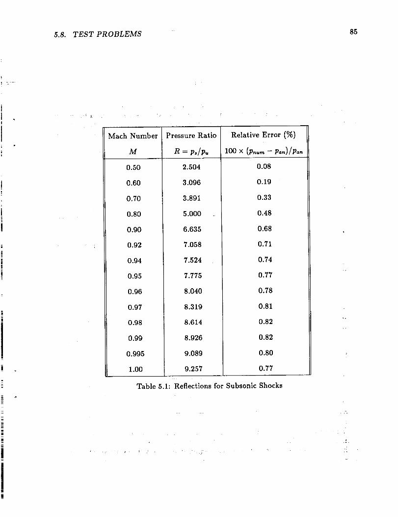
5.8. TEST PROBLEMS 85
Mach Number
M
0.50
0.60
0.70
0.80
0.90
0.92
0.94
0.95
0.96
0.97
0.98
0.99
0.995
1.00
Pressure Ratio
R = po/p_,
2.504
3.096
3.891
5.000
6.635
7.058
7.524
7.775
8.040
8.319
8.614
8.926
9.089
9.257
Relative Error (%)
100 X (Pr*t,m -- Pan)/P,m
0.08
0.19
0.33
0.48
0.68
0.71
0.74
0.77
0.78
0.81
0.82
0.82
0.80
O.77
Table 5.1: Reflections for Subsonic Shocks
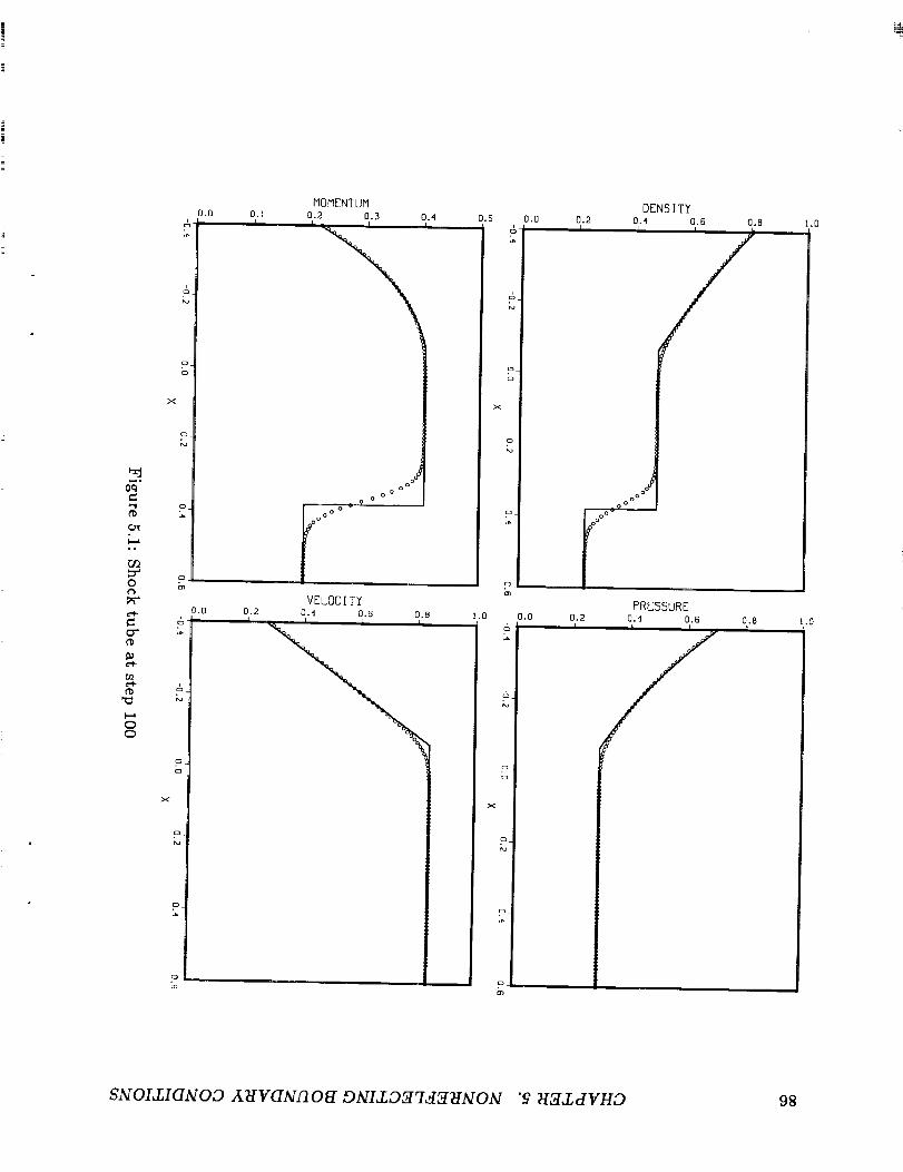
r
o
2_
x
o
0.0 D.I
MOMENTUM
0.2 0.3 0.4
oo °
o ooo i
oq
)=i o |
• - I °°°
=.
_Q
_'_ VELOCITY
_._ 0,0 0.2 0.4 0.6
¢ & ) i r
¢D
00
o
x
p-
ro
0.8 1,0I
D.5 0.0 0.2& r
o
o
x
o
c:3
c3
0,0 0.2
& i,I
I:t
I
:1I
m
DENS]T'f
0.4 0.6 0,8
' '//
oOO s o o °°°°_
PRESSURE
0.4 0,6
f
y0.8
f
1.0
l.O
SNOI,LIGNOD AHVGNI'IOEt DNI, l'.DStq,_45IHNON "_ HSLZdVHD 98
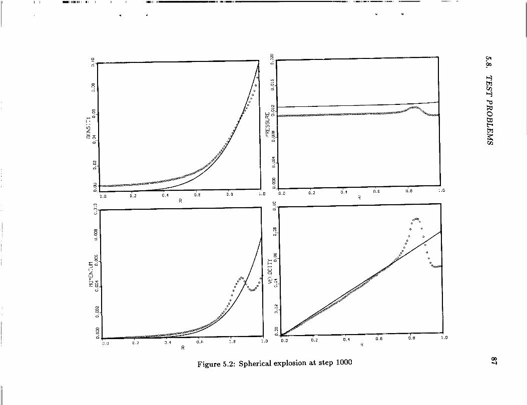
I I
o
c_
c_
o
o
o
ZU
fi::l ._z:c__
o
o.
d
8o
c_
0_
0_00
0.0 0.2 0,_ O.B 0.8
..... _"" "-"" ' ' 01. 80.0 0.2 0.4 0•6
R
o
|
o.
|
4
Z,o7,CO
o |
0.0
o
c;
1.0
o
6
d
oo
.0
oOOOOa
o o
° o o
_ 0
o
0.0 o'.2 0'._ o.6 0'.8R
1.0
60
0
Figure 5.2: Spherical explosion at step 1000
88 CHAPTER 5. NONREFLECTING BOUNDARY CONDITIONS
creased from supersonic (immediately behind the shock) to subsonic. A perturbation
has developed at the boundary and is propagating inward, as can be seen most clearly
from the velocity curve. The discrepancy between the numerical and analytic solutions
is presumably due to the fact that the similarity solution for the explosion really does
contain an inward propagating wave, which is suppressed by the boundary conditions.
The resulting numerical solution is a valid one, but it is not the solution to the explosionproblem at late times.
The impossibility of properly specifying boundary conditions for all problems with the
nonreflecting prescription is further illustrated by the following problem, the homologous
expansion of a uniform medium. At time t = 0 the density and pressure are uniform, with
p -- p = 1. The velocity is linear, with u = X/to, to chosen to be 1. The region studied is
-0.5 < x < 0.5. The density and pressure decrease with time but remain uniform, while
the velocity also decreases but remains linear in x. The flow at the boundaries is alwayssubsonic and directed outward for this set of initial conditions.
The problem has a simple analytical solution, given by
(p = po 1 + , (5.107)
(p = p0 1+ , (5.10s)X
_o
v = t + to (5.109)
One can verify by direct substitution that this solution does not satisfy the nonreflecting
boundary conditions. For example, at the right boundary (x = b) the flow is subsonic
and directed outward. The two characteristic equations representing outgoing waves
(Eqs. (5.56) and (5.57)) hold as written, while the absence of an incoming wave is imposed
by the nonrefIecting condition of Eq. (5.72) with _I -- 0, which can be written
Op i)v
at pc_-( -- O.
The analytic solution does not satisfy the nonreflecting condition, so the nonreflectingcondition will not produce the desired numerical solution.
Figure 5.3 shows the expansion problem at step 50, t = 0.305, with k = 0. The
numerical and analytical solutions diverge markedly near the boundaries, although they
match well in the middle portion. The discrepancy grows with time until the two solutionsdisagree everywhere.
We can use information about this particular problem to specify better boundary
conditions. In particular, the pressure gradient is zero everywhere, and the velocitysatisfies
Ov Ov
o-7+ = 0, (5.110)
which is in characteristic form and describes outflow at the boundary. If (5.110) is used
in place of the nonreflecting boundary condition, we have three characteristic equations
Ji
iIt
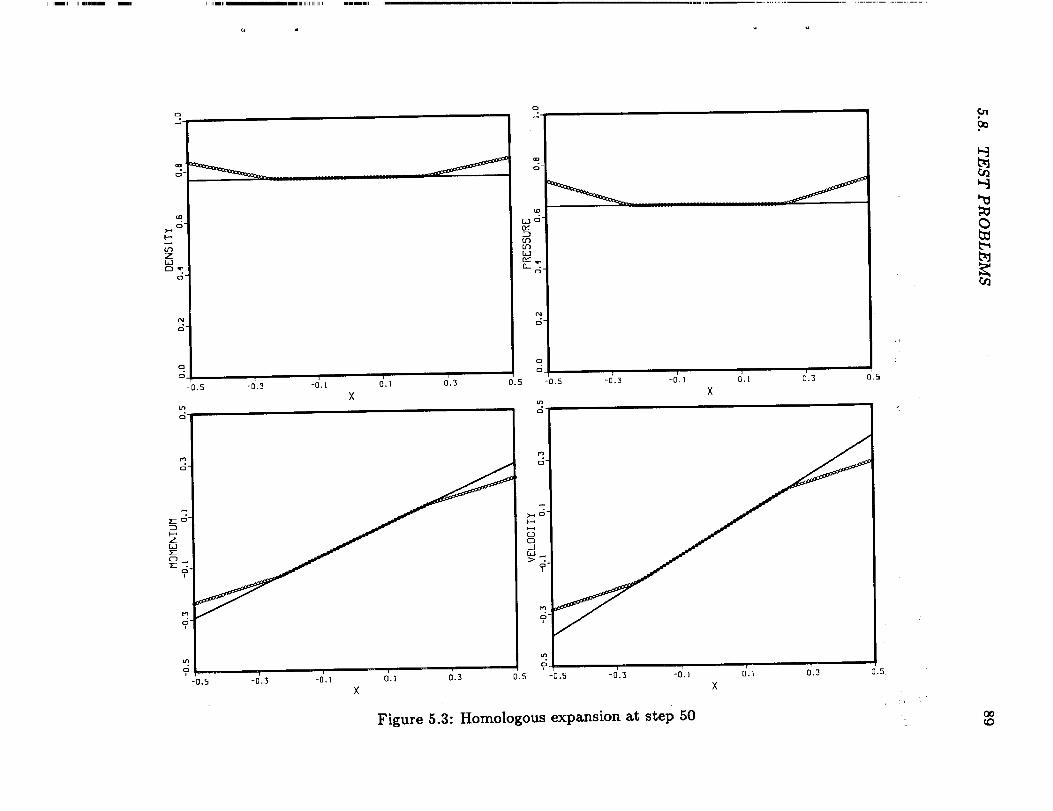
o
o"
ZbJ¢'_I-
d-
o o
_. ,,
o
o
-0.s -0'.3 -_.l 0'._ _._
u_
o-
?-o.s -0'._ -0'._ o'.l 0'.3
o
o-
n,-
b_1
o7
Ol
Ol
0.s -0._ -_._ -0'._ _._ 0'.3
o
,4-
C3--]
o
,,?
u_
,o0,5 -0,5 -0'.3 -0'. 1 0'.i 0'.3
Figure 5.3: Homologous expansion at step 50
0.5
0.5:
r_*q
Ot_t_
00
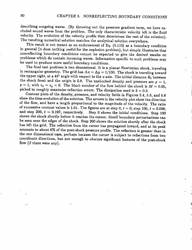
90 CHAPTER 5. NONREFLECTING BOUNDARY CONDITIONS
describing outgoing waves. (By throwing out the pressure gradient term, we have ex-
cluded sound waves from the problem. The only characteristic velocity left is the fluid
velocity. The evolution of the velocity profile then determines the rest of the solution).
The resulting numerical solution matches the analytical solution everywhere.
This result is not meant as an endorsement of Eq. (5.110) as a boundary condition
in general (it does nothing useful for the explosion problem), but simply illustrates that
nonreflecting boundary conditions cannot be expected to give the desired results on
problems which do contain incoming waves. Information specific to such problems maybe used to produce more useful boundary conditions.
The final test problem is two dimensional. It is a planar Newtonian shock, traveling
in rectangular geometry. The grid has _x = Ay _-- 1/130. The shock is traveling toward
the upper right, at a 45 ° angle with respect to the x axis. The initial distance it0 between
the shock front and the origin is 0.8. The unshocked density and pressure are p = 1,
p = 1, with v_ = vy = 0. The Mach number of the flow behind the shock is M = 0.95,picked to roughly maximize reflection errors. The dissipation used is k = 0.3.
Contour plots of the density, pressure, and velocity fields in Figures 5.4, 5.5, and 5.6
show the time evolution of the solution. The arrows in the velocity plot show the direction
of the flow, and have a length proportional to the magnitude of the velocity. The ratio
of successive contour values is 1.01. The figures are at step 0, t -- 0; step 100, t = 0.098;
and step 200, t - 0.197, respectively. Step 0 shows the initial conditions. Step 100
shows the shock shortly before it reaches the corner. Small boundary perturbations can
be seen near the edges of the shock. Step 200 shows the solution shortly after the shock
has left the grid. The reflection from the corner has propagated inward, and at its peak
amounts to about 6% of the post-shock pressure profile. The reflection is greater than in
the one dimensional case, perhaps because the corner is subject to reflections from two
coordinate directions, but not enough to obscure significant features of the post-shockflow (if there were any).
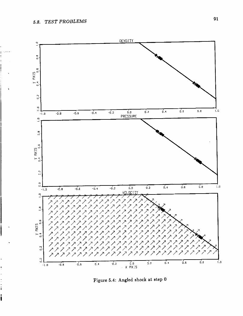
5.8. TEST PROBLEMS 91
o
o-
x
o 4
o
DENSITY
o
o i
-1.o -o'.8 -o'.6 -o'.4 -o'.2 o'.o o'.2 o'.4 o.6 o'.oPRESSURE
o
o
to
X
o-
o
oo
-_.0
o
l,O
00
(fl O"
XEl:
o
r_
o"
o
o
X RXIS
,o
l•O
Figure 5.4: Angled shock at step 0

92 CHAPTER 5. NONREFLECTING BOUNDARY CONDITIONS
oo
o-
x
o-
i::)
-I .0
OEN51TY
o
id-}o
XO:
o-
c_
o
o
-1.0
-o'.8 -o'.6 -0'.4 -&2 d.oPRESSURE
t i-0'.B -0.6 -0.4 -0'.2
×
O'2 O'4 ' 08 10
Figure 5.5: Angled shock at step 100

5.8. TEST PROBLEMS 93
co
O-
X
qr
o"
f_
0"
Q
0
-I.0
0
o
¢0
U-j °
X
_Z
o-
r_
-I.0
R
a0
o
X
0
0
-I.0
DEN51TY
-0'. 8 ' :O..6 -0 '. 4
\
0'.2 0_.4 01.6 0'.8 1.04.2 o..o' PRESSURE
o..o 6.2 o'.4 o'.s o'.e 1.0
-o'.8 -o',6 -o'.4 -o'.2 o'.o O..2 o'.,_ _.s O..e× Axis
1.0
Figure 5.6: Angled shock at step 200
94 CHAPTER 5. NONREFLECTING BOUNDARY CONDITIONS
.
.
,
J
.
.
Exercises
Derive the primitive form of the fluid equations given in Eqs. (5.50) from the
conservative form, in one dimension and in rectangular coordinates.
Starting with Eqs. (5.50), assume isentropic flow (s _-- constant), and show that
only two characteristic equations result. What are the characteristic velocities?
Express the results of problem 2 in the form of Eq. (5.15). The two wave amplitudesV1 and V2 are called Riemana invariaats in fluid dynamics. Each Riemann invariant
is constant along its corresponding trajectory (v - c or v 4- c) in the xt plane.
Riemann invariants do not exist if the flow is non-isentropic.
Find the right eigenvectors of matrix A in Eq. (5.49). Form the similarity transfor-
mation matrices S and S -1, and verify the similarity transformation of Eq. (5.11).
Derive the characteristic velocity components for the two dimensional fluid problemof EQ. (5.61).
Perform the shock wave calculation described in section 5.8, for a Mach number
M = 0.9. Do you see a reflection? If so, how big is it?
Verify that the homologous expansion solution of Eq. (5.107)-(5.109) does not
satisfy the nonreflecting boundary condition at the right boundary.
Appendix A
The Equations of Fluid Dynamics
Chapter 4 described the basic concepts of tensor calculus, the tensor formulation of the
fluid dynamics equations, and artificial viscosity. This appendix provides a complete
list of the relevant equations for fluid dynamics in rectangular, cylindrical, and spherical
coordinate systems.
A.1 Coordinate Geometries and Metric Tensors
The geometry of the coordinate system is described by the metric tensor gab. The metric
tensor is a symmetric second rank tensor, whose components are usually functions of
the coordinates. The metric tensor defines the physical distance ds between two closely
space points, at x" = (x*, x 2, x s) and x _ + dx" = (x 1 + dx 1, x 2 + dx _, x s + dxS), in termsof the coordinate differentials dx% This distance is given by given by
ds 2 = gabdxa dx b. (A.1)
The symmetry of the metric tensor implies that, in n dimensions, only n(n + 1)/2
of its n 2 components may be unique (six components in three dimensions). A general
metric in three dimensions may be written as a 3 × 3 array of numbers,
I gll g12 g13 1
ga b= g21 g22 g23 ' (A.2)
gal gs2 g_3
where by symmetry
gab = gba. (A.3)
In orthogonal coordinate systems, where the coordinate axes are perpendicular to
C_ - _,_ 95
96 APPENDIX A. THE EQUATIONS OF FLUID DYNAMICS
each other, the metric tensor is diagonal, and may be written
where hi, h=, and h3 are the scale factors for the coordinate directions (and the superscript
2 represents the square of the number, not a tensor index).
The covariant derivative of a tensor in coordinate direction a is denoted by the sub-script ;a. The following are useful examples:
aA
A;o = az.' (A.5)
OB"Ba;b = a c (A.6)Ox* + r,,B,
OB,
B.;b = az* r_,B,. (A.7)
ac "b
c"b;_= _O=o + r_oc_ + r_c _d, (A.8)
aC'2b a d
Ca_;c = am c + F&C b - r_cC"d, (A.9)
OCab d : 4 _C,b;, = OX'-----7 ra, c_ - rb, co,_. (A.10)
The connection coefficients F_:, used to evaluate covariant derivatives, are given by
. l(Og,a Ogdc Ogbc_r_° =g"_r_, r_0= _ -0-V+ _ Ox_] ' (A.11)
and are symmetric on the last two indices (F_, = Fc_), due to the symmetry of the metric.
Note that F_ is not itself a tensor. The connection coefficients also satisfy the equation
,, 1 Og 0
Fb,_ -- g Ox _ -- Ox b lng, (A.12)
where g = y/I det(g,b)].
A.2. THE COORDINATE INVARIANT FLUID EQUATIONS 97
A.2 The Coordinate Invariant Fluid Equations
The density (p), pressure (p), and total energy density (e) of a fluid are scalar fields and
are invariant under coordinate transformations. The coordinate velocity (u"), momentum
density (rna = pu, = Pg=_ub), mass flux (pu"), and total energy flux ([e + p]u '_) are vector
(first rank tensor) fields. The momentum flux (pu=ub + psi) is a second rank tensor.The coordinate velocity u ° = dxa/dt is the rate of change of a fluid element coordinate
x" with time, and is generally not the same as the physical velocity v=, which is the rate of
change of distance along coordinate axis x ". In an orthogonal coordinate system, where
the coordinate axes are at right angles to each other, the metric gab is diagonal, with
diagonal elements ga, = h2, • In such a system the physical and coordinate velocities are
related by v= = h=u" (not summed). -'
ClOsing the system =of equations requires auxiliary algebraic equations as well as the
differential equations given below. The relationship between momentum density and
vel0clty is one such equation:
ua = gabUb = gabmb/P" (A.13)
Also useful is the velocity magnitude v, given by
_, __uouo= g,buOu_=_ + _ + _. (A.14)
The equation of state connects the pressure p to the thermal energy density E according
to 1
p= (ff-1)¢, ¢=e-_pv'=e-:m,u=.2 (A.15)
In simple perfect gas problems ff is the ratio of specific heats, and is a constant (equal
to 5/3 for a monatomic gas). In more complicated problems (such as relativistic fluid
dynamics) "_ may be a function of the local fluid state, and is not the ratio of specific
heats.
The equations given in this appendix include dissipative terms for use as artificial
viscosity in finite difference calculations. The dissipation coefficient, _, is taken to be
nonzero only because the grid resolution used in the calculations is finite. To get the
dissipatlon-free equations, simply set _ = 0 throughout. The definition for _ is given in
Chapter 4 and will not be repeated here.
The coordinate invariant fluid equations, with dissipation, are
0p ;= (A.16)_ + (pu");,,= C,_p);,,,
Oe (A.17)a-7+ [(e+ p)u°];°= (_:e;°);.,
Orn, ( _) (A.18)o-V + (m°u_+ p,5_);_= ,_m ;_,in terms of covariant derivatives, or
0p 1 0 ,, 1 0 ( ,,_ 0p'_ (A.19)_7 + ;a-F_.(gp" )- ;o_o _9_g _),

98 APPENDIX A. THE EQUATIONS OF FLUID DYNAMICS
ae 1 a i a f °bae'_c9---[-{- g _x a ig(e -{- p)ua] -- _g_g -_xb )g cgx _ (A.20)
am a
at
1 c9 cgp 1 Og ca
+ g (3xb (gmau b) + ax----_ + _pu,ud ax a
1 a am. rdbm d -- r'_o _'_ \ azbg i)X c gg bct¢ Ox-'-T --
where g = V/[ det(gob)[.
The following sections give the fluid equations explicitly in rectangular, cylindrical,
and spherical coordinates. It should be noted that the forms of the equations given are
not exactly those obtained from the above calculations. Care has been taken to remove
terms which cancel each other (especially when the terms individually become infinite,at singularities) and to cast the equations in a form well suited for finite difference
calculations. The direct translation of the tensor forms given above into finite difference
forms leads to serious cancellation errors. One should always eliminate cancellations
and singularities by hand to the greatest degree possible before resorting to numericalapproximations.
A.3 Rectangular Coordinates
The coordinates are x _ = (x, y, z). The metric and its inverse are
/x]gab = 1
1Is )gab = 1 ,
1
(A.22)
and the metric factor g = 1. The contravariant (coordinate), covariant, and physical
velocities are the same in this (and only this) coordinate system:
,,"= (_:,_,,_),u: = (:_,_,,_),v,, = (_,_,_,)= (u', u,,,,,').
(A.23)
A.3.1 Connection Coefficients
All connection coefficients are zero:
rb_ = O. (A.24)
A.4. CYLINDRICAL COORDINATES 99
A.3.2 The Fluid Equations with Dissipation
Set _ = 0 throughout for the inviscid equations.
Density
Op _._ a v 88_" -t- (pu =) -I- -_y(pu ) + _z(pUs)
- o_ _ +_k _]+_ _
Energy
8e
-- +8t
8 8
x momentum
8rnffi
8t + Cm,_')+ C-%_')+ (m'_') + 8-_
y momentum
8rn v
Ot8 C,-,,,,,,")+ (..,,,u')+ --+ C,,,,,,_')+ _ 8y
= 8-;\ 8_]_\ 8_/_\ 8_/
z momentum
8ms
Ot + ("'"") + (""""") + (""'_') + 8--;
o o o f
A.4 Cylindrical Coordinates
The coordinates are x ° = (r, ¢, z), and are related to rectangular coordinates by
f....-
z = rcos¢, r = _/x2+ y_,
y = r sin ¢, tan ¢ = y/x,
Z= Z_ Z= Z
(A.25)
(A.26)
(A.27)
(A.28)
(A.29)
(A.30)
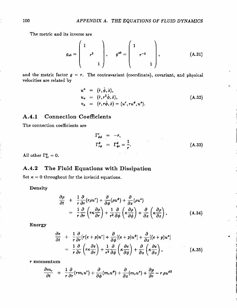
100 APPENDIX A. THE EQUATIONS OF FLUID DYNAMICS
The metric and its inverse are
(1/ l1 /gab : r2 , g,b : r -2 , (A.31)
1 1
and the metric factor g = r. The contravariant (coordinate), covariant, and physical
velocities are related by
,,o = (_,,-_,_)= (.', r._, .').(A.32)
A.4.1 Connection Coefficients
The connection coefficients are
rr
r(A.33)
All other F_ = 0.
A.4.2 The Fluid Equations with Dissipation
Set _ = 0 throughout for the inviscid equations.
Density
Op 1 a _ _ c3O-7 + ;_(_P_ ) + _,_(PU*) + _(P" )
( o,I 1o(o 1_ 1 0 r_-_r +__h _ +r Or r _ 0¢ -_z
Energy
0e 1 0 0_ 0aT + ;_[,(e + p).'] + [(_+ p).*]+ _[(e + p).']
a_ ;zy_ + ,
r momentum
Op _ r pu _2
(A.34)
(A.35)

A.& SPHERICAL COORDINATES 101
|_-z_ ::Yt
momentum
am,
at
z momentum
amz
at
xa f am,_ _ a [ (am,
, )r-_\ Od_ +rm_ ,
4-ap
+_k a_ 1+_ k a_ a_ j'
a (_,u,) ++ (_m,_')+ (_'_*) + _ a,
- , a, k""_-,) + ,-_o-7[,'%-) + _ _, o_j
(A.36)
(A.37)
(A.38)
iI
|
!
|
!@
A.5 Spherical Coordinates
The coordinates are z a = (r, O, _), and are related to rectangular coordinates by
x - r sin 8 cos _, r = Cz 2 + y2 + z 2,
y = r sin 8 sin _, tan 0 -g
z = r cos O, tan _ = V/z
The metric and its inverse are
(A.39)
(1)(1)gob = r _ , g°b = r_ 2 , (A.40)
r 2 sin 2 0 r -2 sin -2 O
and the metric factor g = r' sin 8. The contravariant (coordinate), covariant, and physical
velocities are related by
(A.41)
.. = (_,_,_),.. = (_,.'b,. =sin'o$),v. = (_,rO,rsinO_)= (u',ru°,rsinOu_).
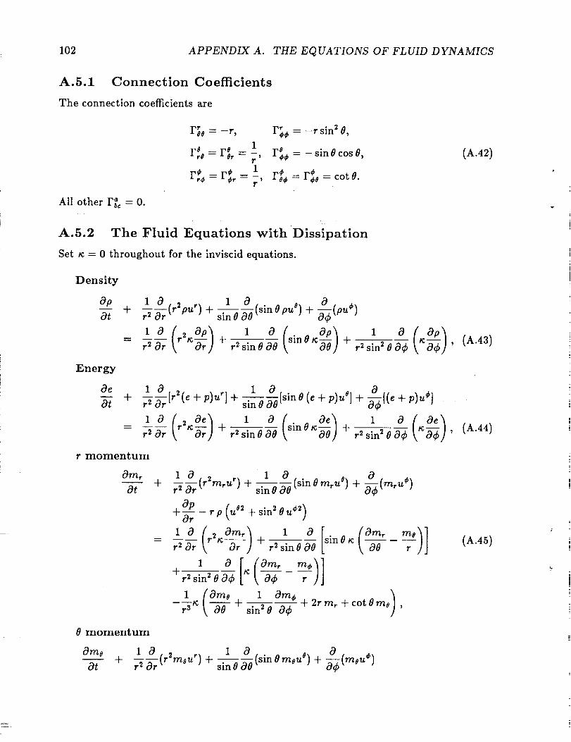
102 APPENDIX A. THE EQUATIONS OF FLUID DYNAMICS
A.5.1 Connection Coefficients
The connection coefficients are
F_0 = -r, r_ = -rsin 2 O,
1r_ = r_, = -, r_, = - sin 0 cos O,
r,**= r_, - _- r_, = r**0= cot 0.
All other r_c = 0.
A.5.2 The Fluid Equations with Dissipation
Set _ = 0 throughout for the inviscid equations.
Density
Op 1 Or 1 0 (sin 0 pu s) + ff-_(pu ¢')O---t + r 2 (r2 pu') + sin000
(0,) 1 0(0,)-- r 20r _r tg_-_-r) nu r2sin0a0 r 2sin 200¢
Energy
0e
o-/+ 1 o _ o [sinO(e+V)uq+_[(e+V)u*}
r 2 o_r r2E -_ r 2 sin0 00 sin 0 t¢_ + r 2 sin 20 0¢ _; '
r momentum
Omr
Ot
0 momentum
+
1 0 (sin0rnrU °) + 0sin0 a0 -0--¢(rn'u ¢')1ont- r2 (r2mrU r) -k
+_rr -rp + sin20
r 20r r2n +r 2sinO00 _ O0
r 2sin 200¢ _k 0¢
1
r 3
me)]
f Omo 1 i)m¢ "_----tz_, 00 +sin 20 0¢ +2rm_+c°t0m°]'
Omo
Ot1 0 (r2mou_) +
-t- r 2 Or 1 0 (sinOmouO) + ff___(mou¢ )sin 0 00
(A.42)
(A.43)
(A.44)
(A.45)
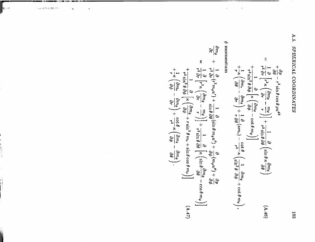
IIII -I-
_ _ ___ _ +
0 ....°t=l e-
+
0
_i __:_ 0
-F
0
-t-
i,.-, °
Q00
_a
0

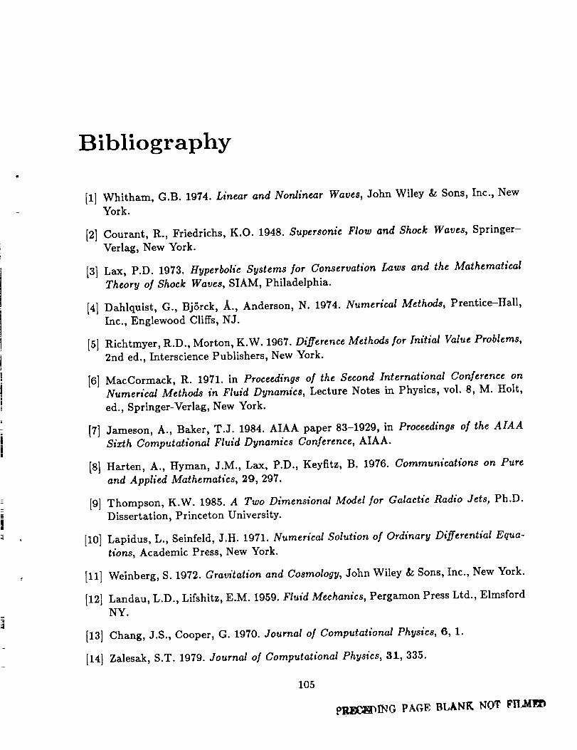
Bibliography
[1] Whitham, G.B. 1974. Linear and Nonlinear Waves, John Wiley & Sons, Inc., New
York.
[2] Courant, R., Friedrichs, K.O. 1948. Supersonic Flow and Shock Waves, Springer-
Verlag, New York.
[3] Lax, P.D. 1973. Hyperbolic Systems for Conservation Laws and the Mathematical
Theory of Shock Waves, SIAM, Philadelphia.
[4] Dahlquist, G., BjSrck, /_., Anderson, N. 1974. Numerical Methods, Prentice-Hall,
Inc., Englewood Cliffs, NJ.
[5] Richtmyer, R.D., Morton, K.W. 1967. Difference Methods ]'or Initial Value Problems,
2nd ed., Interscience Publishers, New York.
[6] MacCormack, R. 1971. in Proceedings of the Second International Conference onNumerical Methods in Fluid Dynamics, Lecture Notes in Physics, vol. 8, M. Holt,
ed., Springer-Verlag, New York.
[7] Jameson, A., Baker, T.J. 1984. AIAA paper 83-1929, in Proceedings of the AIAA
Sixth Computational Fluid Dynamics Conference, AIAA.
[8] Harten, A., Hyman, J.M., Lax, P.D., Keyfitz, B. 1976. Communications on Pure
and Applied Mathematics, 29, 297.
[9] Thompson, K.W. 1985. A Two Dimensional Model for Galactic Radio Jets, Ph.D.
Dissertation, Princeton University.
Lapidus, L., Seinfeld, J.H. 1971. Numerical Solution of Ordinary Differential Equa-
tions, Academic Press, New York.
[11] Weinberg, S. 1972. Gravitation and Cosmology, John Wiley & Sons, Inc., New York.
[12] Landau, L.D., Lifshitz, E.M. 1959. Fluid Mechanics, Pergamon Press Ltd., Elmsford
NY.
[10]
[13] Chang, J.S., Cooper, G. 1970. Journal of Computational Physics, 6, 1.
[14] Zalesak, S.T. 1979. Journal of Computational Physics, 31, 335.
105
p_ING PAGE BLANK NOT PILldl_
106 BIBLIOGRAPHY
[15] Beam, R., Warming, R.F. 1978. AIAA Journal, 16, no. 4, 393.
[16] Shih, T.I-P., Smith, G.E., Springer, G.S., Rimon, Y. 1983. Journal of ComputationalPhysics, 52, 54.
[17] Hedstrom, G.W. 1979. Journal of Computational Physics, 30, 222.
[18] Thompson, K.W. 1987. Journal of Computational Physics, 68, 1.
[19] Jameson, A. 1982. in Transonic, Shock, and Multidimensional Flow: Advances in
Scientific Computing, ed. R. Meyer, Academic Press, New York.
[20] Yee, H.C., Beam, R.M., Warming, R.F. 1982. AIAA Journal, 20, 1203.
[21] Bayliss, A., Turkel, E. 1982. Journal of Computational Physics, 48, 182.
[22] Engquist, B., Majda, A. 1977. Mathematics of Computation, 31,629.
[23] Engquist, B., Majda, A. 1979. Communications on Pure and Applied Mathematics,32,312.
[24] Sod, G.A. 1978. Journal of Computational Physics, 27, 1.
[25] Thompson, K.W. 1986. Journal of Fluid Mechanics, 171,365.

Report Documentation Page
1. Report No.
NASA TM-100010
2. Government Accession No.
4. Title and Subtitle
Lectures Series in Computational Fluid Dynamics
7. Author(s)
Kevin W. Thompson
9. Pedorming Organization Name and Address
Ames Research Center
Moffett Field, CA 94035
12. Sponsoring Agency Name and Address
National Aeronautics and Space Administration
Washington, DC 20546-0001
3. Recipient's Catalog No.
5. Report Date
August 1987
6. Performing Organization Code
8. Performing Organization Report No.
A-87291
10. Work Unit No.
151-02-60-05
11. Contract or Grant No.
13. Type of Report and Period Covered
Technical Memorandum
14. Sponsoring Agency Code
15. Supplementary Notes
Point of Contact: Kevin W. Thompson, Ames Research Center, M/S 245-3
Moffett Field, CA 94035 (415) 694-6275 or FTS 464-6275
16. Abstract
These lecture notes cover the basic principles of computational fluid
dynamics (CFD). They are oriented more toward practical applications than
theory, and are intended to serve as a unified source for basic material in
the CFD field as well as an introduction to more specialized topics in artifi-
cial viscosity and boundary conditions. Each chapter in the text is asso-
ciated with a videotaped lecture; the videotapes may be obtained from the
author.
Chapter I of the notes describes the basic properties of conservation
laws, wave equations, and shock waves. The duality of the conservation law
and wave representations is investigated, and shock waves are examed in some
detail. Chapter 2 introduces finite difference techniques for the solution of
wave equations and conservation laws. Chapter 3 presents stability analysis
for finite difference approximations. Chapter 4 provides a consistent
description of artificial viscosity methods. Finally, Chapter 5 treats the
problem of nonreflecting boundary conditions.
17. Key Words (Suggested by Author(s))
Computational fluid dynamics
CFD, Boundary conditions, Finite
differences, Numerical methods
Artificial viscosity
19. Security Classif. (of this report)
Unclassified
18. Distribution Statement
Unclassified-Unlimited
20. Security classif. (of this page)
Unclassified
Subject Category - 64
21. No. of pages
111
22. Price
A06
NASA FORM 1626 OCT 86
C-P0 788-?86/79016