S F

B XXX

E

C O

N O

M I

C

R

I S

K

B

E R

L I

N

SFB 649 Discussion Paper 2014-030

Forecasting Generalized

Quantiles of Electricity Demand: A Functional

Data Approach

Brenda López Cabrera*

Franziska Schulz*

* Humboldt-Universität zu Berlin, Germany

This research was supported by the Deutsche

Forschungsgemeinschaft through the SFB 649 "Economic Risk".

http://sfb649.wiwi.hu-berlin.de

ISSN 1860-5664

SFB 649, Humboldt-Universität zu Berlin

Spandauer Straße 1, D-10178 Berlin

SFB

6

4 9

E

C O

N O

M I

C

R

I S

K

B

E R

L I

N

Forecasting Generalized Quantiles of Electricity

Demand: A Functional Data Approach. ∗

Brenda López Cabrera, Franziska Schulz†

May 30, 2014

Abstract

Electricity load forecasts are an integral part of many decision-making pro-

cesses in the electricity market. However, most literature on electricity load

forecasting concentrates on deterministic forecasts, neglecting possibly impor-

tant information about uncertainty. A more complete picture of future demand

can be obtained by using distributional forecasts, allowing for a more e�cient

decision-making. A predictive density can be fully characterized by tail mea-

sures such as quantiles and expectiles. Furthermore, interest often lies in the

accurate estimation of tail events rather than in the mean or median. We pro-

pose a new methodology to obtain probabilistic forecasts of electricity load,

that is based on functional data analysis of generalized quantile curves. The

core of the methodology is dimension reduction based on functional principal

components of tail curves with dependence structure. The approach has sev-

eral advantages, such as �exible inclusion of explanatory variables including

meteorological forecasts and no distributional assumptions. The methodol-

ogy is applied to load data from a transmission system operator (TSO) and

a balancing unit in Germany. Our forecast method is evaluated against other

models including the TSO forecast model. It outperforms them in terms of

mean absolute percentage error (MAPE) and achieves a MAPE of 2.7% for

the TSO.

Keywords: Electricity, Load forecasting, FPCAJEL classi�cation: G19, G29, G22, Q14, Q49, Q59

1. INTRODUCTION

With the liberalization of energy markets, the amount of risk borne by operators andmarket participants has increased substantially. Statistical tools can be bene�cial to

∗The �nancial support from the Deutsche Forschungsgemeinschaft via SFB 649 �ÖkonomischesRisiko�, Humboldt-Universität zu Berlin is gratefully acknowledged.†Ladislaus von Bortkiewicz Chair of Statistics, Humboldt-Universität zu Berlin, Spandauer

Straÿe 1, 10178 Berlin, Germany. Email:lopezcab@wiwi.hu-berlin.de,sulzfran@hu-berlin.de

1

assess and manage their risk. Amongst energy, electricity stands out due to its lim-ited storability. Supply and demand have to be balanced out at every point in time.Since electricity is mainly traded in a day-ahead market, short term adjustments insupply due to forecasting errors can lead to enormous �nancial losses. Therefore,load forecasting is extremely important for energy suppliers, transmission systemoperators, �nancial institutions and other participants in electricity market and acrucial process in the planning and operation of electric utilities.

There is a vast literature on how to forecast electricity load, most of them concen-trating on deterministic forecasts. For an overview on common methods see Weron(2007) or Taylor and McSharry (2007). However, for a sustainable risk managementof utility operators not only a forecast of expected demand, but also knowledgeabout the uncertainty and dispersion of future load plays an important role. Thispoints towards the use of probabilistic forecasts. While in di�erent areas of fore-casting such as macro-economics and �nance (Tay and Wallis 2000), meteorology(Leutbecher and Palmer 2008) or renewable energy production (Bremnes 2004; Pin-son et al. 2007) probabilistic forecasts are already well established, there is a lack inliterature on probabilistic forecasts for electricity demand. A notable exception isthe work by Hyndman and Fan (2010) which uses a mixture of temperature simu-lation, economic scenarios, and residual bootstrapping to obtain long-term densityforecasts of electricity demand. Others like Cottet and Smith (2003) use Bayesianmodeling in a multi-equation regression model to forecast intraday electricity loadand brie�y discuss model averaging for probabilistic forecasts.

Short-term probabilistic forecasts yield important information for utility opera-tors for decisions e.g. on purchasing and generating electricity and load scheduling.They are crucial for risk management and can be used to derive risk measures suchas probability of exceedance levels (Taylor 2008; Bellini et al. 2014). In this articlewe propose a methodology to obtain probabilistic forecasts by employing functionaldata analysis of generalized quantile curves.

With generalized quantiles we refer to quantiles (Koenker and Bassett Jr 1978)and expectiles (Newey and Powell 1987). Both are tail measures and uniquelycharacterize the conditional distribution of a random variable. Furthermore, for alarge class of decision-making problems, optimal solutions correspond to quantiles ofa conditional predictive distribution (Gneiting 2011). In fact, in a wide range of �eldsincluding weather events, extreme natural hazards, genomics, risk management,energy demand and portfolio allocation among others, tail indices provide usefulinformation that goes beyond the mean and median. These tail indices constitutecurves that can be treated in a functional principal component analysis (FPCA)context.

The idea of FPCA is to identify the main risk drivers by a small number of factorscombined with random noise. The resulting factors are then to be (cor)related withexogenous variables, which will allow us to study phenomena contingent to extremerisks. Functional data analysis (see Ramsay and Silverman (2005)) is an extensionof multivariate data analysis to functional data. There are few studies that applymethods from functional data analysis to load forecasting, amongst which are Shang(2013), Goia et al. (2010) and Antoch et al. (2008). Others like Cho et al. (2013)reduce dimension using a hybrid approach that combines a generalized additive

2

model for the weekly averages of the load and curve linear regression models for thedependence structure across consecutive daily loads.

Two recent studies on functional data analysis of tail events are Guo et al. (2013),who do the dimension reduction with weighted L1 and L2 norm, where the weightsare sign sensitive, and Tran et al. (2014) who develop an analogue of PCA of tailcurves in an asymmetric norm. However, both studies rely on independence betweenfunctional observations. In many �elds however, such as energy demand modeling,the dependency between curves needs to be taken into account at the core of themodeling. In our study we allow for temporal dependence between functional obser-vations and refer to results from Hörmann and Kokoszka (2010). The dependencebetween tail curves can be exploited for forecasting, which provides useful informa-tion to support modeling, pricing and trading. Our approach has several advantages:It allows for �exible inclusion of explanatory variables and does not require distri-butional assumptions for the tails curves. Furthermore, treating load curves asfunctional data has the advantage that one step ahead forecasts yield forecasts forthe whole next day and that forecasts are continuous functions and thus availablefor every point in time. We expect that exogenous variables like meteorological fac-tors do not only e�ect the amount of electricity consumed, but also the distributionover the day and thus the shape of the load curves (Engel et al. 1986; Harvey andKoopman 1993; Taylor and McSharry 2007).

We illustrate our approach with data on quarter-hourly electricity consumptionof a transmission system operator (TSO) and a balancing unit (BU) in westernGermany. Variations in the intradaily pattern are explained using weather variablesand meteorological forecasts. The proposed model is shown to perform better thanwell-known methods, such as a deterministic similar-day approach, the Holt-WinterExponential smoothing and the forecast provided by TSO Amprion. It achieves onaverage 2.7% mean absolute percentage error (MAPE) in the one-day forecastingperiod for the TSO.

Our article is structured as follows. Section 2 gives a brief introduction of the loaddata. In Section 3 we de�ne FPCA of generalized quantiles that will be used to pro-duce probabilistic load forecasts, together with its estimation algorithm. Section 4discusses the modeling and estimation of the electricity demand data. Section 5 de-scribes the forecast performance with respect to other methods. Section 6 concludesthe paper. All computations in this paper were carried out in R. The electricity loaddata and forecast electricity load data was obtained from TSO Amprion and thebalancing unit Stadtwerke Saarbrücken. The data source for the temperature datais Deutscher Wetterdienst (DWD); for the meteorological weather forecast data thedata source is WeatherOnline. We thank Dr. Ulrich Römer and Herrad Werner forproviding us the data. To simplify notation, in the following dates are denoted withyyyymmdd format. Supplementary materials for this article are available online.

2. ELECTRICITY DEMAND DATA

The German electricity market, which was liberalized in 1998, is Europe's largest,with annual power consumption of around 500 TWh and a generation capacity of125 GW (Eurostat 2014). The four German TSOs (Amprion, Tennet TSO, 50Hertz

3

Transmission and TransnetBW) are responsible for maintaining a stable and reliablesystem and to maintain balance between electricity generation and consumption.All market participants are organized in balancing units (BU). Each BU has a BUmanager who is responsible for the balance within the unit. Electricity is tradedmainly in the day-ahead market, which closes at 12pm. Before, each BU managerhas to submit a load schedule to the corresponding TSO specifying the expectedload for each quarter hour of the next day. Deviations from the speci�ed load canstill be adjusted in the intra-day market. The intra-day market is a continuous mar-ket where contracts can be traded until 45 minutes before delivery. However, theintra-day market is less liquid than the day-ahead market and therefore neglectedin this study. The TSOs balance out di�erences between the forecasted load of theBU and actual consumption in order to ensure a stable system. Precise forecastsof the area's consumption are essential in order to have su�cient capacity avail-able. For deviations between forecasted and actual load BUs have to pay a pricewhich usually greatly exceeds the price at the spot market. Therefore, for BU man-agers improvements in their forecasting performance directly leads to enormous costreductions.

For the empirical work of this article, we use electricity demand data of the TSOAmprion and the BU Stadtwerke Saarbrücken. Both datasets are freely accessibleon their websites. The TSO Amprion operates in the west of Germany. The BUis located within the balancing area of Amprion. The analysis is based on quar-ter hourly data of electricity consumption from 20100101 to 20123112. Summarystatistics are given in Table (1). The �rst two years of the data are used for in-sample �tting and the third year for an out-of-sample forecasting evaluation, givenin Section 5. Figure (1) displays the two load data sets from 2010 to 2012. It isclearly visible that electricity consumption exhibits seasonal features over time andat di�erent times of the day.

Median Mean SD Min Max

TSO 22020 22050 4054.35 11850 34870BU 402 401 95.71 152 630

Table 1: Summary Statistics of the load data (in MW)

It is a stylized fact that it contains yearly, weekly and intraday seasonal cyclesand is sensitive to temperature changes (Engel et al. 1986; Taylor and Buizza 2002).During winter electricity consumption in Germany is higher than during the summer.Additionally, at weekends electricity consumption is usually lower than during theweek. The typical intraday load pro�le shows a peak around noon, followed by valleyin the afternoon and another peak in the evening at around 7pm. These seasonalpatterns are quite predictable and therefore usually modeled deterministically. Weexpress the observed load Ys as

Ys = Λs + Ys, s = 1, . . . , S, (1)

where Λs is a deterministic seasonal component and Ys is a stochastic component.We estimate the deterministic seasonal component separately for every quarter hour

4

Figure 1: Electricity load curves of TSO - Amprion (left) and BU - StadtwerkeSaarbrücken (right) from 20100101 to 20123112.

of a day. It is speci�ed as

Λt,k = at + bt · k + c1,t sin

(2πk

365

)+ c2,t cos

(2πk

365

)+

7∑i=1

di,t ·Di,k, (2)

where t = 1, . . . , 96 denotes the quarter hours of a day and k = 1, . . . , K the day,such that t · k = s. The parameters at,bt,c1,t,c2,t and di,t are estimated by ordinaryleast square regression. Di,k is a set of dummy variables consisting of six dummiesfor the weekdays and one dummy for public holidays. They capture weekly seasonalbehavior, while the sine and cosine functions capture yearly seasonalities. Thisapproach is very close to the so called similar-day approach, which is a commonlyused approach in industry to model and forecast electricity load.

As covariates for load modeling we include average daily temperature and hoursof sunshine. The time series of both variables are displayed in Figure (??). ForSaarbrücken temperature and hours of sunshine are measures from a weather stationin Saarbrücken. For the TSO the average measures of three stations located in theirarea are taken. For forecasting we use meteorological day-ahead forecasts of thecovariates, which are provided by WeatherOnline. For our analysis all covariates aredeseasonalized.

3. METHODOLOGY

We propose a methodology that combines methods from generalized quantile regres-sion and functional data analysis (FDA) in order to obtain probabilistic forecasts ofelectricity demand. FDA has gained importance with the advances in storing largesets of multivariate data. It has been applied in various �elds of research rangingfrom bioscience to medicine and econometrics. For an overview on applications ofFDA we refer to Ramsay and Silverman (2002) or Ferraty and Vieu (2006).

5

Figure 2: Average daily temperature and hours of sunshine for the area of the TSOAmprion (left) and Saarbrücken (right)

3.1 Generalized Quantiles

The distribution of a random variable Y can be characterized by its cdf FY (y). Thequantile functions of Y are de�ned as

QY (τ) = F−1Y (τ) = inf{y : F (y) ≤ τ}, τ ∈ (0, 1). (3)

Like the cdf, the quantile function provides a full characterization of the randomvariable Y . For each τ ∈ (0, 1) the quantile function can be formulated as thesolution of a minimization problem:

QY (τ) = arg miny

E{ρτ (Y − y)}, (4)

where ρτ (·) is a loss function de�ned as

ρτ (u) = u{τ − I(u < 0)}, (5)

which is in general asymmetric (Koenker 2005). A special case is the median, whichcorresponds to τ = 0.5. The quantile function conditional on a (one-dimensional)covariate X is given by

QY |X(τ) = arg minf∈F

E{ρτ (Y − f(X)}, (6)

6

where f(·) is a nonparametric function of the covariate X from a set of functions F ,such that the expectation is well de�ned. Closely related to quantiles are expectilesintroduced by Newey and Powell (1987), which can be obtained by a generalizationof the loss function ρτ (·):

lτ (X) = arg minf∈F

E{ρατ (Y − f(X)}, α ∈ {1, 2} (7)

ρατ (u) = |u|α|τ − I(u < 0)|. (8)

We call the solution of (7) a generalized quantile function. For α = 1 we obtainthe loss function in (5) and the solution to (7) is a conditional quantile function.For α = 2 the solution to (7) is a conditional expectile function. Note that theconditional expectile corresponding to τ = 0.5 is the expected value E(Y |X). Likequantiles, expectiles characterize the distribution of a random variable. While theyare less intuitive to interpret than quantiles, they have the advantage of a bettercomputational e�ciency (Newey and Powell 1987) and are a coherent risk measure(Bellini et al. 2014).

If one is not only interested in estimating a single generalized quantile, but inestimating a collection of generalized quantiles, one faces the problem of crossingquantiles/expectiles. This is unfavorable, since it is theoretically impossible. We usean algorithm proposed by Schnabel (2011), that estimates the generalized quantilefunctions lτ (X) jointly as a surface on the domain of the independent variable Xand the asymmetry parameter τ , called expectile sheet. The algorithm is based ona least asymmetrically weighted squares (LAWS) criterion combined with P-splines.The expectile sheet can be expressed as

µ(X, τ) =K∑k=1

L∑l=1

aklBk(X)Bl(τ), (9)

where B is a B-spline basis for the covariate X, B is a B-spline basis for the asym-metry parameter τ and A = [akl] is a matrix of coe�cients. It is estimated byminimizing

n∑i=1

J∑j=1

wi(τj){Yi − µ(Xi, τj)}2 + P, (10)

where wi(τ) is a weight function and µ(X, τ) is the expectile sheet. P is a penaltyterm de�ned as P = λx||DA||F + λτ ||AD||F , where|| · ||F is the Frobenius norm

and D and D are second order di�erence matrices. The penalty term controls thesmoothness of the estimates and λx and λp are smoothing parameters. The algorithmwas originally developed for expectiles and the weight function wi(τ) is given by

wi(τj) =

{τj if Yi > µ(Xi, τj)1− τj if Yi ≤ µ(Xi, τj).

(11)

With a slight modi�cation the algorithm can be adapted for quantiles as well. Fol-lowing Schnabel and Eilers (2013) the modi�ed weight function is given by

wi(τj) =

τj√

{Yi−µ(Xi,τj)}2+δ2if Yt > µ(Xi, τj)

1−τj√{Yi−µ(Xi,τj)}2+δ2

if Yt ≤ µ(Xi, τj),(12)

7

where δ is a small constant which is used to avoid numerical problems. In thefollowing the covariate X used is time of the day and will be denoted by t.

3.2 Time series of functional data

Electricity demand is recorded in sequential form and shows a similar pattern eachday. Naturally, metered demand can be divided into time intervals of one day.We are interested in generalized quantiles of metered intra-daily electricity demand.The generalized quantile functions de�ned in the previous section can be treatedas realizations lτ,k(t) of a functional time series (lτ,k, k ∈ Z) de�ned on a compactset T and for a �xed τ ∈ (0, 1). For notational convenience we supress τ in thefollowing, i.e. lτ,k(t) := lk(t). Under stationarity lk(t) have a common mean functionE{l(t)} = µ(t) and a common covariance function C(s, t) = Cov{l(s), l(t)} withs, t ∈ T . Note that functional observations are intrinsically in�nite dimensional. Acommon tool to reduce dimensionality is functional principal component analysis(FPCA). For a survey on FPCA we refer the reader to Shang (2014).FPCA yields the directions of largest variability in the data and expresses the data asa weighted sum of the orthogonal principal component functions. If

∫T C(t, t)dt <

∞, the covariance function induces the Kernel operator K : φ 7→ Kφ de�ned by(Kφ)(s) =

∫T C(s, t)φ(t)dt. Then, C has the representation

C(s, t) =∞∑i=0

λiφi(s)φi(t), (13)

where φi for i = 1, 2, . . . are the orthogonal eigenfunctions and λi the correspondingnon-increasing and non-negative sequence of eigenvalues of the operator K. Theeigenfunctions are also called principal component functions. The principal com-ponent scores αi, i = 1, 2, . . . are given by 〈l(t), φi〉, where 〈·, ·〉 denotes the innerproduct. That is, the principal component scores are the projection of l(t) in the di-rection of the corresponding principal component, with E(αi) = 0 and Var(αi) = λi.Using the Karhuhen-Loève expansion we can express each function lk(t) as

lk(t) = µ(t) +∞∑i=1

αikφi(t). (14)

The functions lk(t) can be approximated by a �nite sum of the �rst m principalcomponents, called truncated Karhuhen-Loève expansion:

lk(t) ≈ µ(t) +m∑i=1

αikφi(t) (15)

Note that only the principal component scores are varying over time, whereas themean and principal component functions are time invariant. This observation isexploited for forecasting.

8

3.3 Estimating FPCA for generalized quantiles

In practice the mean, eigenvalues and eigenfunctions are unknown and have to beestimated from the sample. The mean of the functions is estimated by

µ(t) =1

n

n∑k=1

lk(t), (16)

where n is the sample size. We estimate the kernel operator by

(Kφ)(s) =

∫TC(s, t)φ(t)dt, (17)

where

C(s, t) =1

n

n∑k=1

{lk(s)− µ(s)}{lk(t)− µ(t)}. (18)

Estimates of the eigenfunctions and scores are computed from (17) and denoted by φiand αik, i = 1, . . . ,m. Hörmann and Kokoszka (2010) show that these estimates are√n-consistent for a large group of stationary functional time series, which includes in

particular linear functional processes. To choose the number of principal componentfunctions m in Equation (3.2) there exist various rules. Here, the number is chosensuch that at least an a priori �xed amount of variation in the data is explained bythe principal component functions.

3.4 Forecasting functional time series

As noted above, in Equation (14) only the principal component scores α depend ontime, while the common mean function µ and the principal component functionsφ are time-invariant. Hence, the dynamics over time of the load curves are fullycaptured by the dynamics of the principal component scores. The time dynamics ofthe �rst m estimated principal component scores can be modeled using time seriesanalysis (Aue et al. (2014)). The problem of modelling the in�nite dimensionalfunctional data objects reduces thus to modeling a multivariate time series.

In our analysis a vector autoregressive model including exogeneous variables(VARX) turned out to be suitable to capture the dynamics of the principal compo-nent scores. The VARX model of order p is given by

αk =

p∑i=1

Φiαk−i + βxk + ηk (19)

where αk is the vector of estimated principal component scores, Φi is a coe�cientmatrix, xk are exogenous variables and ηk is a white noise process (Lütkepohl 2005).

A forecast of the principal component scores directly yields a forecast of the loadcurve:

lK+h(t) = µ(t) +

m∑i=1

αi,K+hφi(t), (20)

9

where αi,K+h denotes the h-step ahead forecast of the principal component scores

at time K andlK+h(t) is the h-step ahead forecast of the load curve. Although

suitable here, in a more general setting forecast models for the principal componentscores are not retricted to VAR models and can be replaced by many other timeseries models. The next algorithm summarizes the aforementioned steps:Algorithm

1. For �xed τ ∈ (0, 1) and each k = 1, . . . , K, use the data Yt,k, t = 1, . . . , 96 toestimate the k − th generalized quantile curve lτ,k(t) by LAWS

2. Fix m and apply FPCA to lτ,1, . . . , lτ,K :

(a) Compute the empirical mean µ, FPCs φi and FPC scores αk = (α1,k, . . . , αm,k)>,

k = 1, . . . , K, i = 1, . . . ,m

3. For �xed h, use the m−variate time series of empirical FPC scores α =(α1 . . . αm)

>to obtain h−step ahead forecast αK+h = (αK+h,1 . . . αK+h,m)

>

(a) Use a multivariate time series model, e.g. VAR model

(b) Include information from exogenous variables

4. Use αK+h to compute h−step ahead forecast of lK+h as

lK+h(t) = µ(t) +

m∑i=1

αi,K+hφj(t)

3.5 Simulation Study

In this section simualtions are used for illustrating the performance of the proposedmethod for FPCA with generalized quantiles. We run the simulation for indepen-dent as well as autocorrelated functional observations to demonstrate robustness totemporal dependence. For comparison, we follow the simulation setup of Guo et al.(2013) and Tran et al. (2014), who both suggest alternative approaches for modelingfunctional tail event curves. The data Yt,k, k = 1, . . . , K, j = 1, . . . , T is simulatedfrom the model

Yj,k = µ(tj) + α1,kf1(tj) + α2,kf2(tj) + εk,j (21)

where tj are equidistant sampling points in [0, 1] with tj = j/T , µ(t) = 1 +t + exp{−(t − 0.6)2/0.05} is the mean function, f1(t) =

√2 sin(2πt) and f2(t) =√

2 cos(2πt) are the principal component functions and α1,k and α2,k are principalcomponent scores. The principal component scores are generated either (1) indepen-dently from a N(0, 36) and N(0, 9) distribution, respectively or (2) from a VAR(1)process with

Φ1 =

(−0.5 −0.20.2 0.5

).

10

The error εk,t is generated from three di�erent distributions as speci�ed in Table(2), where the �rst one is a light-tailed distribution, the second one is heavy-tailedand the third one exhibits heteroscedasticity. The simulation is run 200 times withtwo di�erent setups: (1) T = 100 grid points per curve and K = 20 curves and(2) T = 150 data points per curve and K = 50 curves. Summary statistics of themean squared errors (MSE) and the average run time in seconds of the simulationsare given in Table (2). The magnitude of the average MSE does not di�er sub-stantially between the independent and the autocorrelated case. This con�rms thatthe quality of the proposed methodology is not sensitive to temporal dependencebetween functional observations. The methodology performs worst for the fat taileddistribution, but well handles heteroscedasticity. Overall, the results are at least asgood in terms of average MSE than those reported by Guo et al. (2013) and Tranet al. (2014).

N = 20, T = 100 N = 50, T = 150(1) (2) (1) (2)

τ = 0.95ε ∼ N(0, 0.5) Mean 0.0448 0.0400 0.0254 0.0233

SD 0.0295 0.0271 0.0174 0.0170AT 3.4400 3.7200 10.1300 11.0100

ε ∼ t(5) Mean 0.2444 0.2290 0.1465 0.1428SD 0.2565 0.2396 0.1590 0.1729AT 3.7500 4.2300 10.3700 12.2500

ε ∼ N(0, µ(t)0.5) Mean 0.0564 0.0518 0.0416 0.0500SD 0.0381 0.0340 0.0286 0.0389AT 3.5100 3.8200 10.2100 11.8000

τ = 0.05ε ∼ N(0, 0.5) Mean 0.0433 0.0407 0.0259 0.0234

SD 0.0285 0.0281 0.0177 0.0168AT 3.3900 3.7200 9.8000 10.3200

ε ∼ t(5) Mean 0.2447 0.2242 0.1480 0.1401SD 0.2508 0.2407 0.1644 0.1571AT 3.7100 4.6600 11.6200 12.0700

ε ∼ N(0, µ(t)0.5) Mean 0.0521 0.0518 0.0499 0.0501SD 0.0379 0.0354 0.0385 0.0393AT 3.2600 3.7700 9.8700 12.2000

Table 2: Mean and standard deviation (SD) of MSE and average run time in seconds(AT) based on K = 200 simulation runs

11

4. MODELING DYNAMICS OF ELECTRICITY

DEMAND

As noted above the generalized quantile functions fully characterize the distribu-tion of electricity demand and they are an alternative to modeling the distributionfunction directly. We model the dynamics of the 1%, 5%, 25%, 50%, 75%, 95% and99% expectile functions using the described functional data approach for the twoyear insample period from 20100101 to 20113112. The expectile functions are ob-tained based on the LAWS algorithm with penalty terms λx and λτ estimated byasymmetric cross validation.

The number of principal components is chosen such that at least 95% of thevariation in the data is explained. Tables (3) and (4) show the explained variation ofeach principal component for all considered expectile levels τ for the BU Saarbrückenand the TSO Amprion, respectively. With four principal components slightly morethan 95% of the variation is captured. For all expectile levels the �rst PC is thedominant factor, explaining roughly three quarter of the variation in the curves.

Expectile level τPC 1% 5% 25% 50% 75% 95% 99%

1 0.7221 0.7223 0.7232 0.7195 0.7247 0.7129 0.72332 0.1209 0.1213 0.1215 0.1220 0.1199 0.1241 0.12273 0.0695 0.0690 0.0687 0.0687 0.0698 0.0691 0.07224 0.0394 0.0409 0.0404 0.0420 0.0416 0.0410 0.0409

Total 0.9521 0.9536 0.9540 0.9524 0.9562 0.9572 0.9593

Table 3: Explained variance of the �rst four principal components for the BU Saar-brücken

Expectile level τPC 1% 5% 25% 50% 75% 95% 99%

1 0.7985 0.7942 0.8007 0.7946 0.7952 0.7956 0.78922 0.0878 0.0893 0.0864 0.0883 0.0892 0.0887 0.09203 0.0583 0.0586 0.0553 0.0559 0.0547 0.0553 0.05414 0.0222 0.0237 0.0240 0.0255 0.0253 0.0252 0.0261

Total 0.9670 0.9659 0.9667 0.9644 0.9645 0.9650 0.9615

Table 4: Explained variance of the �rst four principal components for the TSOAmprion

Figure (3) shows the �rst four principal components for TSO and the BU. Forboth data sets the extracted PCs exhibit similar shapes. The �rst principal compo-nent re�ects variations in the level of electricity load. A positive score on the �rst

12

principal component implies above average consumption, a negative score below av-erage consumption (see Figure (4) for the scores). The second and third principalcomponent capture variations in the height and location of peak load. The steepnessof the load curves is modeled by the fourth principal component.

−2

−1

01

2

Time

PC

1

00:00 06:00 12:00 18:00 24:00

−2

−1

01

2

TimeP

C 2

00:00 06:00 12:00 18:00 24:00

−2

−1

01

2

Time

PC

3

00:00 06:00 12:00 18:00 24:00

−2

−1

01

2

Time

PC

4

00:00 06:00 12:00 18:00 24:00

Figure 3: First four principal components corresponding to τ = 50% of the TSOAmprion (dashed) and the BU (solid)

The load of the TSO is the aggregated load of all BUs located in their areaof responsibility. We compare the dynamics of the principal component scores forτ = 0.5 of the TSO and of the BU Saarbrücken in order to investigate to whichdegree the quantity risk in the BU is driven by the same factors as the overallmarket. The scores of the �rst factor of the TSO and the BU have a correlationof only 0.3 indicating that the level of electricity load of both is only moderatelycorrelated. The correlation of the other scores and di�erent levels of τ is of similarmagnitude.

The dynamics of the principal component scores are modeled by a VARX(p)model. The lag order p is chosen by the Akaike information criterion and equalsp = 7 for all expectile levels. Table (5) shows the estimation results of the exogenousvariables for the TSO. Note that the values refer to deseasonalized data.

Both, daily average temperature and hours of sunshine have a strong negativee�ect on all four principal component scores, implying that they do not only a�ectthe amount of electricity used, but also the allocation over the day. As expected, anincrease in temperature results in lower electricity consumption, since in the area of

13

0 100 200 300 400 500 600 700−30

0020

00

Time

α 1

0 100 200 300 400 500 600 700

−10

050

Time

α 1

0 100 200 300 400 500 600 700−10

0050

0

Time

α 2

0 100 200 300 400 500 600 700

−20

10

Time

α 20 100 200 300 400 500 600 700−

1000

1000

Time

α 3

0 100 200 300 400 500 600 700−20

020

Timeα 3

0 100 200 300 400 500 600 700−40

040

0

Time

α 4

0 100 200 300 400 500 600 700

−10

5

Time

α 4

Figure 4: The scores corresponding to the �rst four principal components ant τ =50% of the TSO Amprion (left) and the BU Saarbrücken (right)

the TSO Amprion there is a high commonness of electric heating in form of night-storage heaters. Similary, more hours of sunshine decrease electricity demand, forinstance due to less demand for lighting and in-house consumption of solar energy.Peak demand is a�ected di�erently by temperature and hours of sunshine as re�ectedin the sign of the coe�cients. While higher temperature causes more pronouncedpeaks, more hours of sunshine �atten the load curve.

For the BU (Table (6)) temperature does not have any e�ect on electricity load.This may be explained by the fact, that the share of electric heating is much lowerin Saarbrücken than in the total area of the TSO. Therefore, demand is less sensitiveto temperature.

In order to test the validity of our model, a multivariate portmanteau test (Hosk-ing 1980) is performed, which suggests to reject the overall signi�cance of residualautocorrelation for lag orders up to 50.

5. FORECAST EVALUATION

In this section we conduct an out-of sample forecast evaluation for the third year ofelectricity consumption data (2012) for the BU and the TSO.

14

α1 α2 α3 α4

τ = 5%Temperature −22.314∗∗∗ −14.805∗∗∗ −11.665∗∗∗ −3.629∗∗

(7.175) (2.903) (2.620) (1.564)Sunshine −24.912∗∗∗ 38.058∗∗∗ 20.184∗∗∗ −6.308∗∗∗

(8.895) (3.599) (3.248) (1.939)τ = 50%

Temperature −22.156∗∗∗ −14.708∗∗∗ −11.276∗∗∗ −3.940∗∗

(7.141) (2.896) (2.591) (1.576)Sunshine −24.563∗∗∗ 38.198∗∗∗ 20.208∗∗∗ −6.059∗∗∗

(8.834) (3.582) (3.205) (1.949)τ = 95%

Temperature −21.892∗∗∗ −13.771∗∗∗ −11.587∗∗∗ −3.790∗∗

(7.187) (2.930) (2.593) (1.557)Sunshine −25.244∗∗∗ 37.850∗∗∗ 21.095∗∗∗ −5.633∗∗∗

(8.877) (3.619) (3.202) (1.923)

Note: ∗p<0.1; ∗∗p<0.05; ∗∗∗p<0.01

Table 5: Estimation Results TSO Amprion. Standard deviation in parenthesis.

α1 α2 α3 α4

τ = 5%Temperature −0.038 −0.039 −0.016 −0.039

(0.154) (0.058) (0.054) (0.041)Sunshine −0.950∗∗∗ 0.633∗∗∗ 0.194∗∗∗ −0.204∗∗∗

(0.191) (0.072) (0.067) (0.051)τ = 50%

Temperature −0.039 −0.037 −0.017 −0.041(0.154) (0.058) (0.054) (0.041)

Sunshine −0.958∗∗∗ 0.631∗∗∗ 0.210∗∗∗ −0.200∗∗∗

(0.190) (0.072) (0.067) (0.051)τ = 95%

Temperature −0.048 −0.036 −0.022 −0.043(0.154) (0.058) (0.055) (0.041)

Sunshine −0.978∗∗∗ 0.627∗∗∗ 0.228∗∗∗ −0.171∗∗∗

(0.190) (0.072) (0.068) (0.050)

Note: ∗p<0.1; ∗∗p<0.05; ∗∗∗p<0.01

Table 6: Estimation Results BU Saarbrücken. Standard deviation in parenthesis ().

15

5.1 Prediction comparison methods

In order to assess the performance of our forecasting approach we compare it tothe results of three di�erent benchmark models. As a �rst benchmark we choosethe simple Deterministic Seasonal Component (DSC) (Eq. 2). The deterministicseasonal component is straightforward to estimate and in modi�ed forms frequentlyused in industry. As a further benchmark we use forecasts that are provided bythe TSO Amprion for their area of responsibility. Additionally, we compare ourmodel to the triple seasonal Holt-Winter exponential smoothing (TSHW) model,which was proposed and applied to short-term load forecasting by Taylor (2010).The latter model accomodates yearly, weekly and daily seasonal cycles and has theadvantage that no speci�cation of the functional form is required. Furthermore,Taylor (2010) shows in an application to data from the UK that the TSHW modeloutperforms simpler exponential smoothing models and performs at least as well asseasonal ARMA models. The formulation of the TSHW model is given by

lt = α(yt − dt−s1 − wt−s2 − at−s3) + (1− α)lt−1 (22)

dt = δ(yt − lt − wt−s2 − at−s3) + (1− δ)dt−s1 (23)

wt = ω(yt − lt − dt−s1 − at−s3) + (1− ω)wt−s2 (24)

at = λ(yt − lt − dt−s1 − wt−s2) + (1− λ)at−s2 (25)

yt+h = lt + dt−s1+h+ wt−s2+h + at−s3+h + φk(yt − lt−1 − dt−s1 − wt−s2 − at−s3) (26)

where lt is the smoothed load, dt, wt and at are seasonal indices for daily, weeklyand annual cycles and α, δ, ω, λ are smoothing parameters. yt+h denotes the h−stepahead forecast at time t and the term including φ is an adjustment for �rst-orderautocorrelation.

5.2 Forecast Results

We evaluate the performance of the proposed forecasting methodology based on theroot mean squared error (RMSE) de�ned as

RMSEh =

√√√√ 1

96

96∑t=1

{lh(t)−lh(t)}2

and the mean absolute percentage error (MAPE) given by

MAPEh =1

96

96∑t=1

| lh(t)−lh(t)

lh(t)|,

where h = 1, . . . , H denotes the day-ahead forecasts. Table (7) reports the mean ofthe RMSE and MAPE based on H = 351 out-of-sample day-ahead forecasts overthe year 2012. Meteorological forecasts of the explanatory variables are used ascovariates. The proposed methodology clearly outperforms the benchmark modelsin terms of the given measures. Surprisingly, also the simple DSC performs relativelygood and yields results similar to those of the TSHW exponential smoothing model.

16

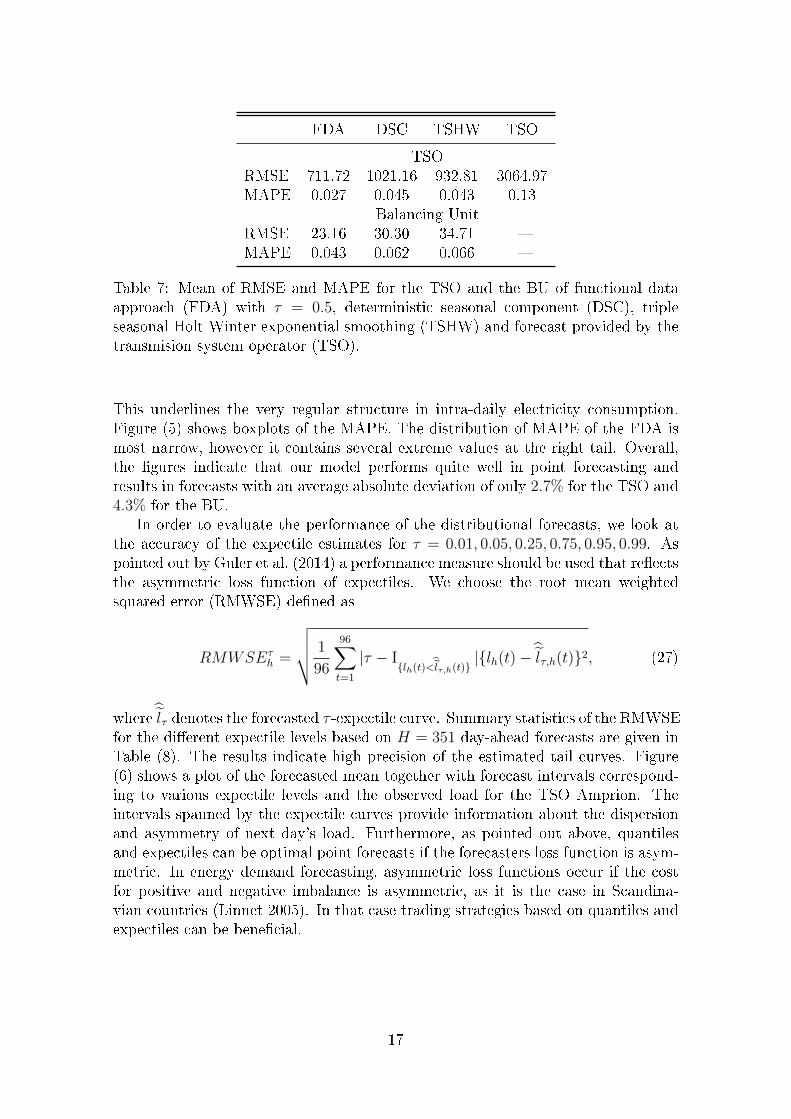
FDA DSC TSHW TSO

TSORMSE 711.72 1021.16 932.81 3064.97MAPE 0.027 0.045 0.043 0.13

Balancing UnitRMSE 23.16 30.30 34.71 �MAPE 0.043 0.062 0.066 �

Table 7: Mean of RMSE and MAPE for the TSO and the BU of functional dataapproach (FDA) with τ = 0.5, deterministic seasonal component (DSC), tripleseasonal Holt-Winter exponential smoothing (TSHW) and forecast provided by thetransmision system operator (TSO).

This underlines the very regular structure in intra-daily electricity consumption.Figure (5) shows boxplots of the MAPE. The distribution of MAPE of the FDA ismost narrow, however it contains several extreme values at the right tail. Overall,the �gures indicate that our model performs quite well in point forecasting andresults in forecasts with an average absolute deviation of only 2.7% for the TSO and4.3% for the BU.

In order to evaluate the performance of the distributional forecasts, we look atthe accuracy of the expectile estimates for τ = 0.01, 0.05, 0.25, 0.75, 0.95, 0.99. Aspointed out by Guler et al. (2014) a performance measure should be used that re�ectsthe asymmetric loss function of expectiles. We choose the root mean weightedsquared error (RMWSE) de�ned as

RMWSEτh =

√√√√ 1

96

96∑t=1

|τ − I{lh(t)<lτ,h(t)}

|{lh(t)−lτ,h(t)}2, (27)

wherelτ denotes the forecasted τ -expectile curve. Summary statistics of the RMWSE

for the di�erent expectile levels based on H = 351 day-ahead forecasts are given inTable (8). The results indicate high precision of the estimated tail curves. Figure(6) shows a plot of the forecasted mean together with forecast intervals correspond-ing to various expectile levels and the observed load for the TSO Amprion. Theintervals spanned by the expectile curves provide information about the dispersionand asymmetry of next day's load. Furthermore, as pointed out above, quantilesand expectiles can be optimal point forecasts if the forecasters loss function is asym-metric. In energy demand forecasting, asymmetric loss functions occur if the costfor positive and negative imbalance is asymmetric, as it is the case in Scandina-vian countries (Linnet 2005). In that case trading strategies based on quantiles andexpectiles can be bene�cial.

17

Expectile level τ1% 5% 25% 50% 75% 95% 99%

TSOMean 566.83 685.42 700.51 711.72 673.97 611.88 496.68SD 440.98 494.81 420.20 416.40 391.32 432.82 373.50

BUMean 13.93 16.82 20.90 23.16 24.47 24.20 23.36SD 6.57 6.71 6.49 7.61 9.31 10.93 11.41

Table 8: Summary Statistics of RMWSE and MAWPE

FDA DSC TSHW TSO

0.00

0.10

0.20

0.30

MA

PE

FDA DSC TSHW

0.00

0.10

0.20

0.30

MA

PE

Figure 5: Boxplot of the mean absolute percentage forecasting error for the TSO(left) and the BU (right) of the functional data approach (FDA), the deterministicseasonal component (DSC), the triple seasonal Holt-Winter exponential smooth-ing model (TSHW) and the forecast provided by the transmission system operator(TSO).

6. CONCLUSION

In this article we show how to get powerful probabilistic short-term forecasts ofintradaily electricity load employing functional data analysis methods with general-ized quantile regression. Probabilistic forecasts yield important information aboutthe uncertainty of future demand and are crucial for sustainable operation of electricutilities and for traders in the electricity market. This novel approach has severaladvantages: It allows for �exible inclusion of explanatory variables and does notrequire distributional assumptions for neither the tails nor the functional form ofthe tail time varying curves. The empirical analysis is based on quarter-hourly datafrom a TSO and a BU in western Germany. The proposed methodology identi�esthe main risk drivers of the electricity load by a number of factors: variations in thelevel of electricity load, variation in the height and location of peak load and thesteepness of the load curves. We show how these factors are then to be (cor)relatedwith climate e�ects.

18

2200

024

000

2600

028

000

Time of day

Load

in M

W

00:00 06:00 12:00 18:00 24:00

Figure 6: Forecasted expected load (black solid line) together with forecasts ofτ = 0.01, 0.05, 0.25, 0.75, 0.95, 0.99 expectiles (gray shades) and observed load (reddashed line) for TSO Amprion on 20120125.

In a forecast comparison study we �nd that our methodology outperforms fore-casts (a MAPE of 2.7%) provided by the TSO as well as those of the benchmarkmodels.

References

Antoch, J., Prchal, L., De Rosa, M. R., and Sarda, P. (2008), �Functional linearregression with functional response: application to prediction of electricity con-sumption,� in Functional and Operatorial Statistics, Springer, pp. 23�29.

Aue, A., Norinho, D. D., and Hörmann, S. (2014), �On the prediction of stationaryfunctional time series,� Journal of the American Statistical Association.

Bellini, F., Klar, B., Müller, A., and Rosazza-Gianin, E. (2014), �Generalized quan-tiles as risk measures,� Insurance: Mathematics and Economics, 54, 41�48.

Bremnes, J. B. (2004), �Probabilistic wind power forecasts using local quantile re-gression,� Wind Energy, 7, 47�54.

Cho, H., Goude, Y., Brossat, X., and Yao, Q. (2013), �Modeling and ForecastingDaily Electricity Load Curves: A Hybrid Approach,� Journal of the American

Statistical Association, 108, 7�21.

Cottet, R. and Smith, M. (2003), �Bayesian Modeling and Forecasting of IntradayElectricity Load,� Journal of the American Statistical Association, 98, 839�849.

Engel, R. F., Granger, C. W. J., Rice, J., and Weiss, A. (1986), �SemiparametricEstimated of the Relation Between Weather and Electricity sales,� Journal of theAmerican Statistical Association, 81, 310�320.

Eurostat (2014), �Supply, transformation, consumption - electricity - annual data,�http://epp.eurostat.ec.europa.eu, accessed: 2014-03-17.

19

Ferraty, F. and Vieu, P. (2006), Nonparametric functional data analysis: theory andpractice, Springer.

Gneiting, T. (2011), �Quantiles as optimal point forecasts,� International Journal ofForecasting, 27, 197�207.

Goia, A., May, C., and Fusai, G. (2010), �Functional clustering and linear regressionfor peak load forecasting,� International Journal of Forecasting, 26, 700�711.

Guler, K., Ng, P. T., and Xiao, Z. (2014), �Mincer-Zarnovitz Quantile and ExpectileRegressions for Forecast Evaluations under Asymmetric Loss Functions,� North-ern Arizona University, Working Paper Series.

Guo, M., Zhou, L., Härdle, W. K., and Huang, J. Z. (2013), �Functional DataAnalysis of Generalized Regression Quantiles,� Statistics and Computing.

Harvey, A. and Koopman, Siem, J. (1993), �Forecasting Hourly Electricity DemandUsing Time-Varying Splines,� Journal of the American Statistical Association,1228�1236.

Hörmann, S. and Kokoszka, P. (2010), �Weakly dependent functional data,� The

Annals of Statistics, 38, 1845�1884.

Hosking, J. R. (1980), �The multivariate portmanteau statistic,� Journal of the

American Statistical Association, 75, 602�608.

Hyndman, R. J. and Fan, S. (2010), �Density forecasting for long-term peak elec-tricity demand,� Power Systems, IEEE Transactions on, 25, 1142�1153.

Koenker, R. (2005), Quantile regression, Cambridge University Press.

Koenker, R. and Bassett Jr, G. (1978), �Regression quantiles,� Econometrica: Jour-nal of the Econometric Society, 46, 33�50.

Leutbecher, M. and Palmer, T. (2008), �Ensemble forecasting,� Journal of Compu-tational Physics, 227, 3515�3539.

Linnet, U. (2005), �Tools supporting wind energy trade in deregulated markets,�Ph.D. thesis, Technical University of Denmark, DTU, DK-2800 Kgs. Lyngby,Denmark.

Lütkepohl, H. (2005), New introduction to multiple time series analysis, Springer.

Newey, W. K. and Powell, J. L. (1987), �Asymmetric least squares estimation andtesting,� Econometrica: Journal of the Econometric Society, 55, 819�847.

Pinson, P., Chevallier, C., and Kariniotakis, G. N. (2007), �Trading wind generationfrom short-term probabilistic forecasts of wind power,� Power Systems, IEEE

Transactions on, 22, 1148�1156.

Ramsay, J. O. and Silverman, B. W. (2002), Applied functional data analysis: meth-ods and case studies, Springer.

20

� (2005), Functional data analysis, Springer.

Schnabel, S. (2011), �Expectile smoothing: new perspectives on asymmetric leastsquares. An application to life expectancy,� Ph.D. thesis, Utrecht University.

Schnabel, S. K. and Eilers, P. H. C. (2013), �Simultaneous estimation of quantilecurves using quantile sheets,� AStA Advances in Statistical Analysis, 97, 77�87.

Shang, H. L. (2013), �Functional time series approach for forecasting very short-termelectricity demand,� Journal of Applied Statistics, 40, 152�168.

� (2014), �A survey of functional principal component analysis,� AStA Advances in

Statistical Analysis, 98, 121�142.

Tay, A. S. and Wallis, K. F. (2000), �Density Forecasting: A Survey,� Journal of

Forecasting, 19, 235�254.

Taylor, J. W. (2008), �Estimating Value at Risk and Expected Shortfall Using Ex-pectiles,� Journal of Financial Econometrics, 6, 231�252.

� (2010), �Triple seasonal methods for short-term electricity demand forecasting,�European Journal of Operational Research, 204, 139�152.

Taylor, J. W. and Buizza, R. (2002), �Neural Network Load Forecasting withWeather Ensemble Predictions,� Power Systems, IEEE Transactions on, 17, 626�632.

Taylor, J. W. and McSharry, P. E. (2007), �Short-term load forecasting methods:An evaluation based on European data,� Power Systems, IEEE Transactions on,22, 2213�2219.

Tran, N. M., Osipenko, M., and Härdle, W. K. (2014), �Principal Component Anal-ysis in an Asymmetric Norm,� Humboldt University Berlin, CRC 649 Discussion

Paper.

Weron, R. (2007), Modeling and forecasting electricity loads and prices: A statistical

approach, Wiley.

21

SFB 649 Discussion Paper Series 2014

For a complete list of Discussion Papers published by the SFB 649,

please visit http://sfb649.wiwi.hu-berlin.de.

001 "Principal Component Analysis in an Asymmetric Norm" by Ngoc Mai

Tran, Maria Osipenko and Wolfgang Karl Härdle, January 2014.

002 "A Simultaneous Confidence Corridor for Varying Coefficient Regression with Sparse Functional Data" by Lijie Gu, Li Wang, Wolfgang Karl Härdle

and Lijian Yang, January 2014.

003 "An Extended Single Index Model with Missing Response at Random" by Qihua Wang, Tao Zhang, Wolfgang Karl Härdle, January 2014.

004 "Structural Vector Autoregressive Analysis in a Data Rich Environment: A Survey" by Helmut Lütkepohl, January 2014.

005 "Functional stable limit theorems for efficient spectral covolatility estimators" by Randolf Altmeyer and Markus Bibinger, January 2014.

006 "A consistent two-factor model for pricing temperature derivatives" by Andreas Groll, Brenda López-Cabrera and Thilo Meyer-Brandis, January

2014.

007 "Confidence Bands for Impulse Responses: Bonferroni versus Wald" by Helmut Lütkepohl, Anna Staszewska-Bystrova and Peter Winker, January

2014. 008 "Simultaneous Confidence Corridors and Variable Selection for

Generalized Additive Models" by Shuzhuan Zheng, Rong Liu, Lijian Yang and Wolfgang Karl Härdle, January 2014.

009 "Structural Vector Autoregressions: Checking Identifying Long-run Restrictions via Heteroskedasticity" by Helmut Lütkepohl and Anton

Velinov, January 2014.

010 "Efficient Iterative Maximum Likelihood Estimation of High-Parameterized Time Series Models" by Nikolaus Hautsch, Ostap Okhrin

and Alexander Ristig, January 2014. 011 "Fiscal Devaluation in a Monetary Union" by Philipp Engler, Giovanni

Ganelli, Juha Tervala and Simon Voigts, January 2014. 012 "Nonparametric Estimates for Conditional Quantiles of Time Series" by

Jürgen Franke, Peter Mwita and Weining Wang, January 2014. 013 "Product Market Deregulation and Employment Outcomes: Evidence

from the German Retail Sector" by Charlotte Senftleben-König, January

2014. 014 "Estimation procedures for exchangeable Marshall copulas with

hydrological application" by Fabrizio Durante and Ostap Okhrin, January 2014.

015 "Ladislaus von Bortkiewicz - statistician, economist, and a European intellectual" by Wolfgang Karl Härdle and Annette B. Vogt, February

2014. 016 "An Application of Principal Component Analysis on Multivariate Time-

Stationary Spatio-Temporal Data" by Stephan Stahlschmidt, Wolfgang

Karl Härdle and Helmut Thome, February 2014. 017 "The composition of government spending and the multiplier at the Zero

Lower Bound" by Julien Albertini, Arthur Poirier and Jordan Roulleau-Pasdeloup, February 2014.

018 "Interacting Product and Labor Market Regulation and the Impact of Immigration on Native Wages" by Susanne Prantl and Alexandra Spitz-

Oener, February 2014.

SFB 649, Spandauer Straße 1, D-10178 Berlin http://sfb649.wiwi.hu-berlin.de

This research was supported by the Deutsche

Forschungsgemeinschaft through the SFB 649 "Economic Risk".

SFB 649, Spandauer Straße 1, D-10178 Berlin http://sfb649.wiwi.hu-berlin.de

This research was supported by the Deutsche

Forschungsgemeinschaft through the SFB 649 "Economic Risk".

SFB 649, Spandauer Straße 1, D-10178 Berlin http://sfb649.wiwi.hu-berlin.de

This research was supported by the Deutsche

Forschungsgemeinschaft through the SFB 649 "Economic Risk".

SFB 649 Discussion Paper Series 2014

For a complete list of Discussion Papers published by the SFB 649,

please visit http://sfb649.wiwi.hu-berlin.de.

019 "Unemployment benefits extensions at the zero lower bound on nominal

interest rate" by Julien Albertini and Arthur Poirier, February 2014.

020 "Modelling spatio-temporal variability of temperature" by Xiaofeng Cao, Ostap Okhrin, Martin Odening and Matthias Ritter, February 2014.

021 "Do Maternal Health Problems Influence Child's Worrying Status? Evidence from British Cohort Study" by Xianhua Dai, Wolfgang Karl

Härdle and Keming Yu, February 2014.

022 "Nonparametric Test for a Constant Beta over a Fixed Time Interval" by Markus Reiß, Viktor Todorov and George Tauchen, February 2014.

023 "Inflation Expectations Spillovers between the United States and Euro Area" by Aleksei Netšunajev and Lars Winkelmann, March 2014.

024 "Peer Effects and Students’ Self-Control" by Berno Buechel, Lydia Mechtenberg and Julia Petersen, April 2014.

025 "Is there a demand for multi-year crop insurance?" by Maria Osipenko, Zhiwei Shen and Martin Odening, April 2014.

026 "Credit Risk Calibration based on CDS Spreads" by Shih-Kang Chao,

Wolfgang Karl Härdle and Hien Pham-Thu, May 2014. 027 "Stale Forward Guidance" by Gunda-Alexandra Detmers and Dieter

Nautz, May 2014. 028 "Confidence Corridors for Multivariate Generalized Quantile Regression"

by Shih-Kang Chao, Katharina Proksch, Holger Dette and Wolfgang Härdle, May 2014.

029 "Information Risk, Market Stress and Institutional Herding in Financial Markets: New Evidence Through the Lens of a Simulated Model" by

Christopher Boortz, Stephanie Kremer, Simon Jurkatis and Dieter Nautz,

May 2014. 030 "Forecasting Generalized Quantiles of Electricity Demand: A Functional

Data Approach" by Brenda López Cabrera and Franziska Schulz, May 2014.