r - - _ a 1 1

I I

I OAK RIDGE ' NATIONAL I

I

LABORATORY . I

Variable-Density Flow And Transport Modeling To Evalaute

Anomalous Nitrate Concentrations And Pressures in GW-134

L O C K H E E D I

T. L. Jones L. E. Toran

D. B. Watson

MANAGED AND OPERATED BY LOCKHEED MARTlN ENERGY RESEARCH CORPORATION S ni~l ; r~t~~rr 'o~ r\F THIS DOCUMENT IS UNLIMITED FOR THE UNITED !%TATS DEPARTMENT OF ENERGY

ORNL-27 0

This report has been reproduced directly from the best available copy.

Available to DOE and DOE contractors from the Office of Scientific and Technical Information. P. 0. Box 62, Oak Ridge, TN 3783 1; prices available from (423) 576-840 1, FTS 626-8401.

Available to the public from the National Technical Information Service, U.S. Department of Commerce, 5285 Port Royal Road, Springfield. VA 221 61.

This report was prepared as an account of work sponsored by an agency of the United States Government. Neither the United States Government nor any agency thereof, nor any of their employees. makes any warranty, express or implied, or assumes any legal liability or responsibility for the accuracy, completeness, or usefulness of any information, apparatus, product, or process disclosed. or represents that its use would not infringe privately owned rights. Reference herein to any specific commercial product, process, or service by trade name, trademark. manufacturer, or otherwise, does not necessarily constitute or imply its endorsement, recommendation, or favoring by the United States Government or any agency !hereof. The views ilnd opinions of authors expressed herein do not necessarily state or reflect those of the United States Government of any agency thereof.

DISCLAlMER

Portions of this document may be illegible in electronic image products. Images are produced from the best available original document.

.- .

ORNL/GWPO-0024

Variable-Density Flow And Transport Modeling To Evaluate Anomalous Nitrate Concentrations

And Pressures in GW-134

T. L. Jones L. E. Toran

D. B. Watson

June 1996

Prepared by Environmental Sciences Division Oak Ridge National Laboratory

Prepared for the U.S. Department of Energy

Office of Environmental Restoration and Waste Management under budget and reporting code EW 20 10 30 2

OAK RIDGE NATIONAL LABORATORY Oak Ridge, Tennessee 3783 1-6285

managed by LOCKHEED MARTIN ENERGY RESEARCH COW.

for the U.S. DEPARTMENT OF ENERGY

under contract number DE-AC05-960W2464.

VARIABLE-DENSITY FLOW AND TRANSPORT MODELING TO EVALUATE ANOMALOUS NITRATE CONCENTRATIONS

AND PRESSURES IN GW-134

by Toya L. Jones

INTERA Inc, Austin, Texas and

Laura Toran and David Watson Lockeed Marietta Energy Research, Environmental Sciences Division,

Oak Ridge National Laboratory

J NTR ODU CTI ON

The U.S. Department of Energy operates the Oak Ridge Reservation near Oak

Ridge, Tennessee. Four waste disposal ponds, referred to as the S-3 ponds, were

located within this reservation near the western edge of the Y-12 Plant. The S-3 ponds

were constructed in 1951 and received liquid waste until 1983. The main component of

the waste received by the ponds was nitric acid. In 1988, the ponds were structurally

stabilized and capped and the area above the ponds was converted into an asphalt

parking lot.

In 1985, four coreholes were drilled west of the S-3 ponds to characterize the

geology of the region. These four coreholes were later equipped with a multiport

monitoring and sampling system. The multiport system is capable of collecting

pressure measurements from numerous zones and contains seven to ten additional

zones from which fluid samples can also be collected. Data collection from the

multiport systems began in 1990. The pressure measurements and fluid sample

analyses from the multiport system installed in one of the coreholes (GW-134) appear

to be anomalous. The distance between GW-134 and the center of the S-3 ponds is

approximately 600 ft at the surface and approximately 800 ft along dip in the

1

subsurface. Figure 1 is a schematic of the relative positions of the S-3 ponds and

GW-134. The pressure data from GW-134 indicates a pressure bulge in the central

portion of the well at a depth of about 450 f? and the sample analyses indicate a

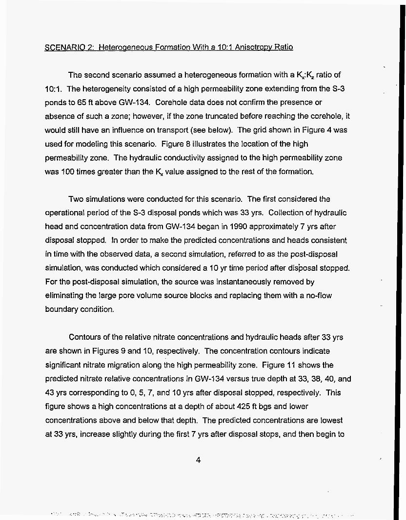
maximum nitrate concentration near the crest of the pressure bulge (Dreier et al., 1993). Figure 2 shows head data collected from GW-134 in July 1991 and Figure 3

shows nitrate concentration data collected from GW-134 in January 1991. This data as

well as data from other sampling periods will be discussed in this report. The depths in Figures 2 and 3 are true depths below ground surface. A detailed discussion of the

pressure and concentration data collected from all four coreholes can be found in Dreier et al. (1993).

I

The modeling study presented here was conducted to evaluate scenarios potentially capable of producing the apparently anomalous pressure and concentration

data observed in GW-134. The purpose of the modeling was to determine a hydraulic conceptualization in the vicinity of the S-3 ponds and GW-134 that would produce

pressures and concentrations at the location of GW-134 that were consistent with the

observed data. This study was scoping in nature and was not designed to provide a

detailed representation of the physical system. The modeling presented here is an

extension of work by L. Toran (Environmental Sciences Division, ORNL).

Included in the modeling was the density difference between the native fluid and

the liquid disposed of into the S-3 ponds. The native fluid has a density of 62.4 lb/ft3

(1.00 g/cm3) and the waste has a density of 66.8 lb/ft3 (1.07 g/cm3). Also included was

the 45 degree dip of the formation underlying the S-3 ponds. A two-dimensional x-z model with the x-direction tilted 45 degrees was used. The four S-3 ponds were

combined into a single source having a length of 400 ft across the ground surface (see

Figure 1). The source was simulated using grid-blocks with very large pore volumes

and an initial waste concentration of 1 .O. Treating the S-3 ponds in this manner

ensured a constant source over the time period of the simulations. Two different model

2

grids were used for this study. The two grids are illustrated in Figures 4 and 5. The

model boundary conditions consisted of a constant hydraulic head of 990 ft along the

top side of the model based on a regional model constructed in the area (Toran and

Saunders, 1992). There was a constant hydraulic head of 1010 ft along the bottom

side of the model (see Figure I) and no-flow conditions at all other boundaries. The

constant heads were included in the model in order to incorporate the natural

groundwater gradient oriented perpendicular to the formation dip in the direction toward

ground surface. The following sections discuss results for model simulations

conducted to evaluate the influence of selected heterogeneity and anisotropy in the

hydraulic conductivity (K) on plume and pressure head development. The three

scenarios considered were: 0 a homogeneous formation with a &:K, ratio of 1O: l 0 a heterogeneous formation with a &:% ratio of 1O:l 0 a homogeneous formation with a &:K, ratio of 1OO:l

SCENARIO 1: Homoaeneous Formation With a 1O:l Anisotropv Ratio

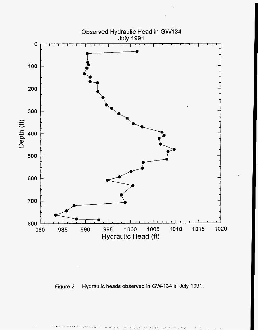
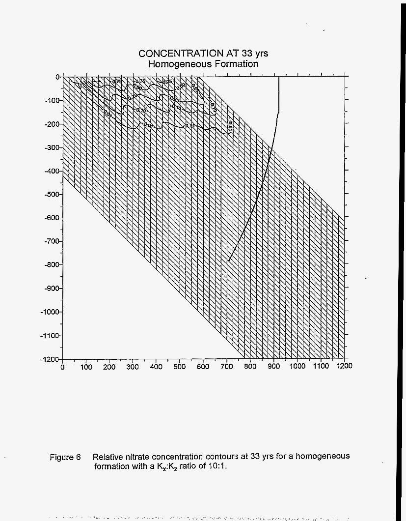
The first scenario assumed a homogeneous hydraulic conductivity with a %:& ratio of 1O:l. A hydraulic conductivity of 8.64 x I O ” ftlday was assumed in the x- direction. This value is consistent with that used by Toran and Saunders (1 992) in their

regional flow model for the Y-12 Plant. The grid shown in Figure 4 was used for this

modeling. Figure 6 shows the relative concentration contours for nitrate at the end of

33 yrs of disposal and the location of GW-134. The results indicate that after 33 yrs of

migration the plume does not intersect GW-134. Contours of the hydraulic head after

33 yrs along with the location of GW-134 are given in Figure 7. This figure shows no

effect on the hydraulic heads at GW-134 due to the 33 yrs of disposal into the S-3

ponds. For this scenario, the observed concentration and pressure data cannot be

reproduced using a homogeneous conceptualization with K, and K, values consistent

with previously conducted regional flow modeling of the site.

3

, . , . ,- c . -- - J ~ - - - .--. . ___ . %

. . , ,

SCENARIO 2: Heteroaeneous Formation With a 1O:l Anisotropv Ratio

The second scenario assumed a heterogeneous formation with a q:)(L ratio of

1O: l . The heterogeneity consisted of a high permeability zone extending from the S-3 ponds to 65 ft above GW-134. Corehole data does not confirm the presence or

absence of such a zone; however, if the zone truncated before reaching the corehole, it

would still have an influence on transport (see below). 'The grid shown in Figure 4 was

used for modeling this scenario. Figure 8 illustrates the location of the high

permeability zone. The hydraulic conductivity assigned to the high permeability zone

was 100 times greater than the K, value assigned to the rest of the formation.

Two simulations were conducted for this scenario. The first considered the operational period of the S-3 disposal ponds which was 33 yrs. Collection of hydraulic

head and concentration data from GW-134 began in 1990 approximately 7 yrs after

disposal stopped. In order to make the predicted concentrations and heads consistent

in time with the observed data, a second simulation, referred to as the post-disposal

simulation, was conducted which considered a 10 yr time period after dis'posal stopped.

For the post-disposal simulation, the source was instantaneously removed by eliminating the large pore volume source blocks and replacing them with a no-flow

boundary condition.

Contours of the relative nitrate concentrations and hydraulic heads after 33 yrs

are shown in Figures 9 and I O , respectively. The concentration contours indicate

significant nitrate migration along the high permeability zone. Figure 11 shows the

predicted nitrate relative concentrations in GW-I 34 versus true depth at 33, 38, 40, and

43 yrs corresponding to 0, 5, 7, and 10 yrs after disposal stopped, respectively. This

figure shows a high concentrations at a depth of about 425 ft bgs and lower

concentrations above and below that depth. The predicted concentrations are lowest

at 33 yrs, increase slightly during the first 7 yrs after disposal stops, and then begin to

4

decrease.

Sampling on January 28, 1991 indicates a nitrate concentration of 5520 mg/L in zone 18 which is 415 to 437 ft bgs (Dreier et ai., 1993). The highest nitrate

concentration reported in the monitoring well is 14,270 mg/L at around 482 ft (June

1992, R.B. Dreier, personal communication). Shevenell et al. (1994) indicate that the

typical nitrate concentration in the liquid waste was about 50,000 mg/L. This yields an

observed relative concentration of 0.1 1 for the January 28, 1991 measurement and

0.29 for the highest measured concentration. Both of these values are significantly

lower then the relative concentration of about 0.77 predicted for this time period (see

Figure 1 I). This indicates that including a high permeability zone having the properties

discussed above results in a greater degree of migration than is observed. The trend

of the predicted concentrations from the post-disposal simulation is consistent with the

observed data which indicates no decrease in nitrate concentration since sampling

began.

The predicted hydraulic heads in GW-134 versus true depth at 33, 38,40, and

43 yrs corresponding to 0, 5, 7, and I O yrs after disposal stopped, respectively, are

shown in Figure 12. This figure shows a pressure bulge in the region between depths

of about 300 and 500 ft bgs. The slight difference in the location of the maximum

concentration and the maximum head in Figures 11 and 12, respectively, is a function

of the averaging process required for plotting the data due to the combination of a tilted

grid and a curved corehole.

The model predicts a head of about 995 ft in the pressure bulge at 7 yrs after

disposal stopped which is lower than the observed maximum of about 1012 ft. Figure 12 shows that the predicted hydraulic heads decrease significantly during the

first 7 yrs after disposal stops and then decrease only slightly between 38 and 43 yrs.

The initial head decrease is due to pressure equilibration which occurs very rapidly as

5

a result of unloading the system by removing the source blocks in the post-disposal

simulation. Observed data is not available at the time disposal into the S-3 ponds

ended. Therefore, the model predicted heads at the end of disposal cannot be

compared to observed head data. Furthermore, the post-disposal head data are affected by installation of packers in the monitoring well, which disturbs the pressure

locally. The observed head data collected between 1990 and 1994 (7 to 11 yrs after

disposal stopped) shows maximum heads varying between about 101 2 and 1000 ft

amsl. The predicted heads during this time period at the location of the bulge decrease

from about 996 to 995 ft. Thus, the predicted heads are lower than the observed heads

and the predicted rate of head decline is slower than the observed rate. Some factors

that can account for these differences include the instaritaneous removal of the source

term in the post-deposition model (which affects loading, as discussed below), lack of

observational data immediately following remediation, and the influence of packers on

local pressure data following installation of monitoring zones.

Additional simulations were conducted in which the hydraulic conductivity of the

high permeability zone was varied to between 10 and 50 times higher than the K, of the

remainder of the formation. The purpose of these simulations was to determine

whether the model predicted relative concentration at a depth of 425 ft could be

reduced to a level near the observed relative concentration at that depth. These

simulations indicated that the predicted relative concentration was too low (0.0) for a

factor of ten increase in the hydraulic conductivity and was still high (0.30) for a factor

of 11 increase. The simulations also showed that the predicted hydraulic head at this

depth decreased as the hydraulic conductivity of the high permeability zone decreased.

Therefore, any reduction in the hydraulic conductivity of the high permeability zone

decreased both the relative nitrate concentration, which was desirable, and the

hydraulic head, which was undesirable since it was already too low with a factor of 100

increase in hydraulic conductivity.

6

These results indicated that the existence of a high permeability zone from the

S-3 ponds to 65 ft above GW-134 could produce both a high concentration and a

pressure bulge in GW-134 at a location consistent with the observed data. However, a

hydraulic conductivity for the high permeability zone which produced a consistent

hydraulic head overpredicted the relative nitrate concentration and, likewise, a

hydraulic conductivity which produced a consistent relative concentration

underpredicted the hydraulic head measured in the packer intervals.

The simulations conducted here assumed only one configuration for the

hypothesized high permeability zone. That is, an approximately 20-ft thick zone

extending from directly below the S-3 ponds to 65 ft above GW-134. If other

configurations had been considered, the magnitude of the nitrate concentration and the

pressure bulge predicted by the model would change. Although not modeled, a shorter

high permeability zone (Le., truncating at a shallower depth and/or beginning at a deeper depth) would result in lower concentrations and pressures, a longer zone (Le.,

truncating closer to GW-134) would result in higher concentrations and pressures, a

thicker zone would result in elevated concentrations and pressures extending over a larger portion of GW-134, and a thinner zone would result in elevated concentrations

and pressures extending over a smaller portion of GW-134.

The true vertical distance between pressure measurement ports in GW-134

ranges from about 4.5 to 42 ft. Across the location of the observed pressure bulge, the

true vertical distance between pressure measurement ports ranges from about 10 to

34 ft. The distances to the measurement ports immediately above and below the measurement port having the highest pressure measurement in July 1991 (see

Figure 2) are about 10 and 34 ft, respectively. This suggests that the uncertainty in the

location of the highest measured pressure is about 44 ft. However, since the pressure

bulge is defined by a large number of sampling points, the uncertainty in the overall

location of the observed pressure bulge is presumed to be small.

7

The true vertical distance between pumping ports in GW-134 ranges from about

65 to 190 ft. The distances to the pumping ports immediately above and below the pumping port location with the highest nitrate concentration measurement in July 1991

(see Figure 3) are 137 and 146 ft, respectively. This suggests that the uncertainty in the location of the highest observed nitrate concentration is about 283 ft. In addition,

there is also uncertainty in the value of the highest nitrate concentration. The true peak

concentration could be located in between the packer sampling points, and thus be

greater than the maximum concentration observed from the point sampling.

SCENARIO 3: Homoaeneous Formation With a 1OO:l Anisotropv Ratio

The final set of simulations assumed a homogeneous hydraulic conductiw ty wii

a K,& ratio of 1OO:l. The grid shown in Figure 5 was used to model this scenario.

The initial simulations were conducted using a K, consistent with the regional flow

model (Le., 8.64 x I O ” ftlday). These results indicated no concentration or pressure

increase in GW-134.

decreased the extent of downdip migration. The degree of migration is a function of

both the x-direction hydraulic conductivity, which is tilted 45” down from horizonal, and

the vertical hydraulic conductivity. Maintaining a constant and decreasing $ results

in an overall decrease in the hydraulic conductivity controlling migration.

Increasing the anisotropy ratio from 10:l (scenario A ) to 1OO:l

A series of simulations was conducted to determine a K, at which a

concentration increase would be predicted in GW-134 for a 1OO:l anisotropy ratio.

Based on these simulations, K, and )(L values of 4.32 x I O 2 and 4.32 x I O 4 Wday,

respectively, were selected. Both operational period and post-disposal simulations

were conducted for this scenario.

Figure 13 shows the predicted relative concentration contours and Figure 14

shows the predicted hydraulic head contours for this scenario. The concentration

8

contours in Figure 13 show two "fingers". A great deal of effort was put into

determining whether these "fingers" were an actual result of the model or were caused

by numerical problems due to the way the model handled the formation tilt. This was

tested by incorporating the formation tilt into the model using an alternative method. A

brief description of this alternative method is provided in Appendix A. The results using

the alternative method also showed "fingering" in the concentration contours. This

indicated that the "fingers" were not caused by numerical problems but were instead a

valid result of the model.

Development of the "fingers" occurs due to the upward migration of the lighter

formation fluid in the central region of the source. The formation fluid then gets trapped

below the center of the source and the heavier contaminant fluid migrates around the

trapped lighter fluid. The lighter formation fluid does not move to the left of the source

because, due to the tilt of the formation, migration in that direction would require

horizontal movement before vertical movement could begin. On the other hand, the

lighter formation fluid moves upward below the center of the source because movement

in that direction requires only a vertical component. The development of the trapped

lighter formation fluid is a function of both the large source width and the two- dimensional model. Simulations indicate that the fingering does not develop if the

source width is significantly reduced. In addition, the directions which the lighter

formation fluid can move as it is displaced by the heavier fluid from the source is

restricted because the model is only two dimensional rather than three dimensional.

A 2-dimensional modeling study conducted by Zhang and Schwartz (1 995) with a

surface source containing fluid more dense than the ambient formation fluid shows

"cells" within their plume. The development of these cells may be the result of a similar

phenomenon where the lighter formation fluid is trapped as it is displaced by the

denser contaminant.

Figure 15 shows the relative nitrate concentrations in GW-134 versus true depth

at 33, 38, 40, and 43 yrs representing times of 0, 5, 7, and 10 yrs after disposal

9

stopped, respectively. For this scenario, the predicted relative concentrations continue

to increase after disposal stops. The maximum predicted concentrations are higher

and are located at a shallower depth than the observed maximum concentrations. The

highest relative concentration observed for GW-134 is 0.29 calculated from

concentration measurements from June 1992 about 9 yrs after disposal stopped. The

predicted concentration for this time period is about 0.5.

Figure 16 shows the hydraulic heads in GW-134 versus true depth at 33, 38, 40,

and 43 yrs representing times of 0, 5, 7, and 10 yrs after disposal stopped,

respectively. This figure shows two bulges at depths which correspond to the depths of the two concentration "fingers". The predicted hydraulic: heads decrease significantly

between 33 and 38 yrs but change only slightly between 38 and 43 yrs. The decrease

predicted between 33 and 38 yrs is a result of the boundary conditions assumed for the

source. For the post-disposal simulation, the source was instantaneously removed and

replaced with a no-flow boundary. Removing the source in this manner removes a load

from the system and causes rapid dissipation of the pressures.

A second post-disposal simulation was conducted in which the source was not

instantaneously removed to determine the effects of removing the load from the system

(as was done in the post-disposal simulation discussed above) on the predicted

hydraulic heads. This simulation maintained the source and, consequently the load it

applied, but converted the fluid in the source from dense waste to fresh water. This

was done by maintaining the large pore volume source blocks but changing their

concentration from 1 .O (contaminant fluid) to 0.0 (fresh water). In effect, this created a

zone of fresh-water recharge at the location of the S-3 ponds. The post-disposal heads

predicted by this simulation increased with time in contrast to the results shown in Figure 16 which decreased with time. The behavior of the plume predicted by this

post-disposal simulation was consistent with the behavior predicted by the post-

disposal simulation in which the source was totally removed. Both simulations

predicted plume growth and increasing concentrations in GW-134 with time after

disposal stopped.

10

. .. . .

SUMMARY AND CONCLUSIONS

A series of simulations was conducted to determine a mechanism which could

explain the anomalous nitrate concentrations and pressure bulge observed in GW-I 34. The simulations incorporated the density drive developed due to the density difference

between the heavier waste fluid from the S-3 ponds and the lighter formation fluid.

Also incorporated in the modeling was the 45 degree dip of the formation underlying

the S-3 ponds and the natural hydraulic gradient perpendicular to the formation dip in the upward direction. Three scenarios for the formation underlying the S-3 ponds were

considered. The first was a homogeneous formation with a &:K, ratio of 10:l. Using a

)5( consistent with the regional flow model, the model predicted no nitrate concentration

or pressure bulge in GW-134. Although it was not simulated, a nitrate concentration and a pressure increase in GW-134 could have been obtained if the yC value had been

increased by some factor, but probably not using realistic values.

The second scenario was a heterogeneous formation with a &:& ratio of 1O:l. The heterogeneity was in the form of a high permeability zone extending from the S-3 ponds to 65 ft above the location of GW-134 along the dip of the formation. The

position of the high permeability zone was consistent with the depth in GW-134 at

which the high nitrate concentration was observed. This scenario yielded high relative

nitrate concentrations and a pressure bulge at a depth of about 425 ft bgs in GW-134. These results indicated that the magnitude of the relative concentration and the

pressure bulge were dependent upon the value of the hydraulic conductivity assigned

to the high permeability zone. As the hydraulic conductivity of the high permeability

zone was increased, the magnitude of both the relative concentration and pressure

also increased. Also indicated by these simulations was that a hydraulic conductivity in the high Permeability zone which yielded relative concentrations near the observed

value underpredicted the magnitude of the pressure bulge.

11

The third scenario assumed a homogeneous formation below the S-3 ponds

with a &:& ratio of 1OO:l. These simulations yielded relative concentration "fingers" due to the entrapment of lighter formation fluid under the center of the source. These

"fingers" developed due to the large width of the source and the limitation in flow direction caused by the two-dimensional model. Pressure bulges were predicted at

the locations of the concentration "fingers".

Neither post-disposal simulation for scenario 3 (source instantaneously removed

and fresh-water recharge blocks) was consistent with actual conditions during

decommissioning of the S-3 ponds. However, they did bound those conditions which consisted of continued recharge during the time period when the fluid in the ponds was denitrified and removal of the liquid in the S-3 ponds prior to paving the area for a

parking lot. Since the two alternative treatments of the source for the post-disposal

simulations do not represent actual conditions, the pressure responses after disposal

stopped have not yet been captured by the modeling. Although the method in which the source is treated for the post-disposal simulations has a significant impact on the

pressure response, it has very little impact on the predicted concentrations.

Therefore, it is not considered to be a source of discrepancy between the higher predicted concentrations and the lower observed concentrations.

The simulations presented here indicate that the apparently anomalous nitrate

concentrations and pressure bulge observed in GW-134 can be explained by migration

due to density drive in a formation with a 45 degree dip. Inclusion of a hydraulic

gradient perpendicular to the formation dip in the direction toward ground surface

indicates that the transport velocities due to density drive are greater than those due

to the background gradient. Consequently, the resultant direction of waste migration is downward along the dip of the formation. The schematics of the system indicate that, for downward migration along dip, the distance from the right edge of the source to the middle portion of GW-134 is shorter than the distance from the left edge of the

source to the lower portion of GW-134 (about 500 ft versus about 1000 ft). Therefore,

12

contaminant intersected the middle section of GW-134 more quickly than it will intersect the lower section of GW-134.

The simulations discussed here indicate that the general trend of the observed data from GW-134 can be reproduced assuming a homogeneous formation with anisotropy in the & (along bedding) to permeability zone between the S-3 ponds and GW-134. In general, the degree of nitrate contamination w a s overpredicted and the magnitude of the pressure bulge w a s underpredicted by these simulations. The scenario assuming a 1003 anisotropy ratio

hydraulic conductivity and assuming a high

could not be quantitatively evaluated d u e to limitations of the two-dimensional model, but anisotropy alone is a viable hypothesis to consider. These simulations suggest that the nitrate concentrations and pressure bulge observed in GW-134 are not anomalous but can be explained with reasonable assumptions regarding stratigraphy and contaminant density.

REFERENCES

Dreier, R.B., T.O. Early, and H.L. King. 1993. Resulfs and lnferprefafion of Groundwafer Data Obtained from Mulfiport-lnstrumentd Coreholes (G W- 13 I fhrough GW-735), Fiscal Years 7990 and 7991. YKS-803. Oak Ridge, TN: Martin Marietta Energy Systems, Inc.

Toran, L.E., and J.A. Saunders. 1992. Geochemical and Groundwafer Flow Modeling of Mulfiporf-lnsfrumenfed Coreholes (G W-13 I through G W-135). YKS-895. Oak Ridge, TN: Martin Marietta Energy Systems, Inc.

Shevenell, L.A., G.K. Moore, and R.B. Dreier. 1994. "Contaminant Spread and Flushing in Fractured Rocks Near Oak Ridge, Tennessee", Ground Wafer Moniforing Review, Spring 1994, pg 120-129.

13

Zhang, H., and F.W. Schwartz. 1995. "Multispecies Contaminant Plumes in Variable Density Flow Systems". Water Resources Research, Vol. 31 , No. 4, pgs 837-847.

14

S-3 PONDS GW-134 / 620 f t - - 400 ft-

Figure 1 Schematic illustration of the relative location of the S-3 ponds and G W- 1 34.

Observed Hydraulic Head in GWI34 July I991 fi o ~ " " " " ' " l " ' ' -

I

t

995 1000 1005 I010 1015 1020 800 I

980 985 990 Hydraulic Head (ft)

Figure 2 Hydraulic heads observed in GW-134 in July 1991.

1

- - . , .. ,. . .... "- . _, ... , ~ . . . - 7 . . . . . I _ .- .I . : . :- * I " .. , A. - . . . :

Figure 3 Nitrate concentrations observed in GW-134 in January 1991.

Model Grid for Homogeneous and Heterogeneous Formation Simulations With a n Anisotropy Ratio of 1O: l

~

-1 000

-500

0

500

1000 - *

2000

2500

3000

3500

3

0 500 1000 1500 2000 2500 3000 3500 4000 4500 5000 Horizontal Distance (ft)

Figure 4 Model grid used for the homogeneous and heterogeneous simulations with a K,:K, ratio of 1O:l .

Model Grid for Homogeneous Formation Simulations With an Anisotropy Ratio of 1OO: l

-500

0

500

1000 n 4-J

Lc, 5 1500 Q

E 2000

2500

3000

3500

4000 0 500 1000 1500 2000 2500 3000 3500

Horizontal Distance (ft)

Figure 5

I

Model grid used for the homogeneous simulations with a K,:K, ratio of 1OO:l.

CONCENTRATION AT 33 yrs Homogeneous Formation

Figure 6 Relative nitrate concentration contours at 33 yrs for a homogeneous formation with a K,:K, ratio of 1 O : l .

HEAD CONTOURS AT 33 yrs Homogeneous Formation

I 1 1 I

500.00 1000.00 1500.00 200b.00 250b.00 300;

Figure 7 Hydraulic head contours a t 33 yrs for a homogeneous formation with a K,:K, ratio of 1O: l .

Figure 8 Location of the high permeability zone for the heterogeneous formation simulations with a K,:K, ratio of 1O: l .

RELATIVE CONCENTRATION AT 33 yrs High K (K*lOO) Layer from Source to 65 ft Above GW-I 34

Figure 9

13404 FBC.S RF

Relative nitrate concentration contours at 33 yrs for a heterogeneous formation with a KxXz ratio of 1O:l.

HEAD CONTOURS AT 33 yrs High K (K*I 00) Layer from Source to 65 ft Above GW-134 -

00

1344EFHD.SRF

Figure 10 Hydraulic head contours a t 33 yrs for a heterogeneous formation with a KxXz ratio of IO:?.

RELATIVE CONCENTRATION IN GW-134 High K (K*IOO) Layer from Source to 65 ft Above GW-134

0 I I I I I I I 1 I I I I 1 I I I I 1 I - - - - 33 yrs

38 yrs - 40 yrs

_------__-_-_ -

- r-1: 43 yrs

I 0 0 -

200 - - - - - -

300 - - - - - - - -

400 - - - - - - -

- -

- - -

600 - - - - - - - -

700 - - - - - - - -

800 - I I 1 1 I I I I I I I I I I I I I I I

0.0 0.1 0.2 0.3 0.4 0.5 0.6 0.7 0.8 0.9 1.0 Relative Concentration

Figure 11 Relative nitrate concentrations in GW-134 at 33, 38, 40, and 43 yrs after disposal into the S-3 ponds began for a heterogeneous formation with a K,:K, ratio of 1O:l .

0 1 1 " ~ " ' ~ ' ' " ~ ' " ' ~ ' " ' ~ " "

- - - - 33 yrs

38 yrs --_----_----- - - 40 yrs - [L] ; 100 -

200 - - - - - -

300 - - - - - - -

- -

400 - - - - - -

500 - - - - - - - -

600 - - - - - - - -

700 - - - - - - -

1 1 1 1 1 1 1 1 1 1 1 1 1 I , I l l 1 1 1 1 1 . I , , I l l 1 800 ' I I I I

970 975 980 985 990 995 1000 1005 I010 1015 1020

Figure 12 Hydraulic heads in GW-134 a t 33, 38, 4.0, and 43 yrs after disposal into t h e S-3 ponds began for a heterogeneous formation with a K,:K, ratio of 1O:l.

Figure 13 Relative nitrate concentration contours at 33 yrs for a homogeneous formation with a K,:K, ratio of 1OO:l.

0.00

-500.00

-1000.00

-1500.00

-2000.00

-2500.00

-3000.00

HEAD CONTOURS AT 33 yrs 1OO:l Anisotropy - Kx=4.32E-2 ft/day; Kz=4.32E-4 Wday

I 500.00 100b.00 150b.00 200b.00 250b.00 3001 00

Figure 14 Hydraulic head contours at 33 yrs for a homogeneous formation with a K,:K, ratio of 1OO:l .

RELATIVE CONCENTRATION IN GW-134 1OO: l Anisotropy - Kx=4.32E-2 ft/day; Kz=4.32E-2 Wday

0 - 1 I I I I I I 1 I 1 I I I I 1 I I

- - - - - -

100 - - - - - - - -

200 - - - - - - - - - -

- - 500 - -

- -

- - - - - -

- -

700 - - - - - - - -

800 I I I 1 1 I 1 1 I I I I I I I I I I I

gwl34bac.grf

Figure 15 Relative nitrate concentrations in GW-134 at 33, 38,40, and 43 yrs after disposal into the S-3 ponds began for a homogeneous formation with a Kx:K, ratio of 1OO:l.

--- -I-

.- --

HYDRAULIC HEAD IN GW-134 1OO:l Anisotropy - Kx=4.32E-2 Wday; Kz=4.32E-4 Wday

970 975 980 985 990 995 1000 1005 I010 1015 1020 Hydraulic Head (ft)

Figure 16 Hydraulic heads in GW-134 at 33, 38, 40, and 43 yrs after disposal into the S-3 ponds began for a homogeneous formation with a K,:K, ratio of 1OO:l.

Appendix A

Comparison of the Alternative Method for Incorporating Formation Dip (Rotated Grid) to the Method Used (Tilted Grid)

The simulations conducted for this report used the SWIFT I I code. This code

allows for direct input of a reservoir dip angle for both the x and y axes. The

simulations presented in the report used this option to tilt the x-axis 45 degrees from

horizontal. Tilting the grid using this method constitutes a non-orthogonal

transformation and yields x- and z-directions which are no longer perpendicular to

each other. The transformed x-direction is oriented 45 degrees from horizontal and

the z-direction retains its vertical orientation. The resultant locations of the grid-block

centers for this grid, referred to as the tilted grid, are illustrated in Figure Al .

When plume fingering was observed in the Scenario 3 results, it was

speculated that the fingering could be due to numerical problems caused by the tilted

grid. The first potential problem was calculation of the x-direction dispersive transmissivities using untilted rather than tilted distances between grid-block centers.

The second potential problem could have been caused by the calculation of

transverse dispersion in the tilted grid where the x and z axes were not perpendicular.

To test this hypothesis, an alternative approach was implemented. A preprocessor

was used to rotate the grid by an angle 8=45 degrees using the transformation:

Assuming that the coordinate origin is coincident with the axis of rotation, this

transformation determines coordinate locations (x',z') in the rotated system as

functions of their locations (x,z) in the unrotated system. Block-center coordinates z'

were input using the depth-modification option of SWIFT 11. The locations of the grid-

block centers for this grid, referred to as the rotated grid, are illustrated in Figure A2.

15

Using the rotated grid eliminated potential problems of the tilted grid by maintaining an orthogonal grid with perpendicular x' and z' axes.

The results obtained using the rotated grid (Figure A3) showed fingering within the plume just as the results obtained using the tilted grid had shown. The overall

shape of both plumes was essentially the same. The most notable difference between

the two results was the distance of migration. The distance predicted using the

rotated grid (about 545 ft for the upper finger) was about 34 percent less than that predicted using the tilted grid (about 830 ft for the upper finger). This confirmed that

the fingering observed in the simulated results was not caused by numerical problems but was a valid result of the modeling.

16

-500

0

500

L

0 500 1000 1500 2000 2500 3000 3500 4000 4500 5000 Horizontal Distance (ft)

Figure A1 Location of grid-block centers for tilted grid.

4 0 0 0 t ~ ~ ' " " " ' ' " " " ' " " ' " " " ~ 0 500 1000 1500 2000 2500 3000 3500 4000 4500 5000

Horizontal Distance (ft)

Figure A2 Location of grid-block centers for rotated grid.

RELATIVE CONCENTRATION AT 33 yrs 1OO:l Anisotropy - Kx=4.32E-2 Wday; Kz=4.32E-4 Wday

Rotated Grid 0 I I I 1 I 1 I I I I I

-1 00-

-200-

-300-

-400-

-500-

-600-

-700-

-800-

-900-

-1000-

-1100-

0

Figure A3 Relative nitrate concentration contours at 33 yrs for a homogeneous formation with a K,:K, ratio of 1OO:l using the rotated grid.

. , .. . ..~ ~. . . .. . _ . _ ,,_. I

>

INTERNAL DISTRIBUTION

1. F. A. Anderson, X7725, MS-7615

3. L. D. Bates, K-1001, MS-7169 4. H. L. Boston, 7078-A, MS-6402 5. A. J. Caldanaro, 1509, MS-6400 6. R. B. Clapp, 1509, MS-6400

8. T. K. Cothron, K-1001, MS-7155

10. V. H. Dale, 1505, MS-6035 1 1. A. F. Diefendorf.. 1509, MS-6400 12. R. B. Dreier, 1509, MS-6400

2. L. V. A s p h d , K-1330, MS-7298

7. R. B. Cook, 1505, MS-6038

9. J. H. C ~ ~ h m a n , 1059, MS-6422

13. T. 0. Early, 1509, MS-6400 14. N. T. Edwards, 1059, MS-6422 15. D. E. Fowler, 1505, MS-6035 16. C. W. Gehrs, 1505, MS-6036 17. C. S. Haase, K-1330, MS-7298 18. S. G. Hildebrand, 1505, MS-6037

20. G. K. Jacobs, 1505, MS-6036 21. W. K. Jago, 9207, MS-8225 22. P. Kancircuk, 1507, MS-6407 23. R. H. Ketelle, 4500-N, MS-6185 24. H. L. King, 99830AH, MS-8247

19. D. D. Huff, 1509, MS-6400

25. A. J. Kuhaida, 7078-A, MS-6402 26. P. J. Lemiszki, 1509, MS-6400

28. G. R. Moline, 1509, MS-6400 29. J. C. Powers, X7725, MS-7615 30. D. E. Reichle, 4500N, MS-6253 3 1. C. T. Rightmire, 1509, MS-6400 32. W. E. Sanford, 1509, MS-6400 33. F. E. Sharples, 1505, MS-6036 34. S. D. Shriner, 1505, MS-6038

36. L. E. Toran, 1509, MS-6400 37. D. B. Watson, 1509, MS-6400 38. S. L. Welch, 1001, MS-7155 39. S. L. Winters, 1509, MS-6400 40. M. W. Yambert, 4500-N, MS-6243 41. T. F. Zondlo, 1509, MS-6400 42. Central Research Library 43-58. ESD Library 59-60. Laboratory Records Department 61. Laboratory Records, ORNL-RC 62. ORNL Patent Section 63. ORNL Y-12 Technical Library

27. J. M. LO=, 1505, MS-6036

35. S. H. Stow, 1505, MS-6035

EXTERNAL DISTRIBUTION

64. R. Benfield, Tennessee Department of Environmental Conservation, U.S. Department of Energy Oversite Office, 76 1 Emory Valley Road, Oak Ridge, TN 3783 1

65. G. W. Bodenstein, U.S. Department of Energy, Oak Ridge Operations Ofice, IRC Building, P.O. Box 2001, Oak Ridge, TN 37838-8541

66. M. Broido, Acting Director, Environmental Sciences Division, Department of Energy, 19901 Germantown Road, Germantown, Maryland 20874

67. F. A. Donath, Director, Institute for Environmental Education, Geological Society of America, 1006 Las Posas, San Clemente, California 92673

68. D. W. Freckman, Director, College of Natural Resources, 1001 Natural Resources Buildings, Colorado State University, Fort Collins, Colorado 80523

69. Paul Hofmann, U.S. Department of Energy, Oak Ridge Operations Office, P.O. Box 2001, Oak Ridge, Tennessee 37838-8541

70. Larry D. McKay, University of Tennessee, Department of Geology, 306 G&G Building, Knoxville, Tennessee 37996-1410

71. A. Patrinos, Associate Director, Office of Health and Environmental Research, Department of Energy, G- 165, Germantown, Maryland 20874

72. G. S . Sayler, Professor, 105 15 Research Drive, Suite 100, The University of Tennessee, Knoxville, Tennessee 37932-2567

73. D. K. Solomon, University of Utah, Department of Geology and Geophysics, 717 W. C. Browning Building, Salt Lake City, Utah 841 12-1 183

74. F. J. Wobber, Environmental Sciences Division, Office of Health and Environmental Research, ER-74, Department of Energy, 19901 Germantown Road, Germantown, Maryland 20874

75. Chris Provost, CDM Federal, 800 Oak Ridge Turnpike, Suite 500, Oak Ridge, Tennessee 37830

76. Duncan MOSS, SAIC, 301 Laboratory Road, Oak Ridge, Tennessee 37830

77. Toya Jones,. INTERA, Inc., 6850 Austin Center Boulevard, Suite 300, Austin, Texas 78731

78. Office of Assistant Manager for Energy Research and Development, U.S. Department of Energy Oak Ridge Operations, P.O. Box 2001, Oak Ridge, Tennessee 37831-8600

79-80. Office of Scientific and Technical Information, P.O. Box 62, Oak Ridge, Tennessee 3783 1

~~

Please do not forward or discard this document.

if this address is not correct for the designated addressee, please return the document to:

Oak Ridge National Laboratory, ESD/GWPO P.O. Box 2008

Building 1509, MS-6400 Oak Ridge, Tennessee 37831-6400