PLUSED NUCLEAR MAGNETIC SPIN RESONANCELast Revised: August 8, 2007

QUESTION TO BE INVESTIGATED:

THEORY:The physics behind NMR/MRI signal production lies in the physics of spin.

This section will cover enough aspects of spin to understand the generation of NMR signals. Although this initial spin discussion is inherently quantum mechanical in nature, we will later need to employ some simple principles from thermodynamics and classical dynamics to further describe the art of NMR. These topics will be thrown into this discussion in an ad hoc manner when necessary.

Spin is a specific (internal) manifestation of angular momentum inherent in physical entities. All of the basic constituents of matter (and the constituents of known forces apart from gravity) possess a definite value of spin. Because spin is a notoriously quantum mechanical property, it is naturally “quantized” in discrete, not continuous, values. These values, the possible spin quantum numbers, exist as integer (for bosons) and half-integer (for fermions) values. The symbol most often used to represent the nuclear spin quantum number is the symbol I.

Spin itself can be represented in a complex vector space, with the magnitude of a given spin state expressed in terms of a spin quantum number. This relation is given as

)1( += IIS hr 1.0

Where ћ is Planck’s constant divided by 2. A simultaneously observable quantity in addition to the magnitude of S is the component of S along one arbitrary axis, usually denoted as “z”. This Sz value also takes on integer and half-integer values of ћ, with the integer value specified by the quantum number m. The possible values of m run from –I to I in unit steps. Thus, if I = ½ , the only possible values for m are – ½ and ½, giving Sz values of –ћ/2 and

ћ/2 respectively. I = ½ turns out to be the simplest nontrivial manifestation of spin, and the present case of interest.

The spin of a charged particle may be easily observed due to its magnetic moment. The spin and magnetic moment of a particle are proportional to each other by a factor known as the gyromagnetic ratio, .

Srr μ = 1.1

The gyromagnetic ratio of nuclei consisting of only a single proton, turns out to be relatively large (2.675x108Hz/T) compared to the gyromagnetic ratios of other NMR active nuclei (Liang, 59), and therefore creates a larger (more observable) magnetic moment for the same value of S. Due to their , hydrogen nuclei are the nuclei most responsible for NMR effects in research and clinical imaging. The hydrogen nucleus, a single proton, has I= ½. The following paragraphs discuss the role of this spin in the production of NMR signals.

Let us use the analogy of a spinning top. If a top is placed on a table with any component of its axis of rotation offset from vertical, then the top will begin to wobble, or more precisely, precess in a circle about the vertical axis.

Let us denote the vertical axis as z. The rate of precession about z can be found given the rate of change of the angular momentum vector, L. This quantity is defined as the torque, t= rCM x W, which is exerted by the force of gravity, mg=W, at the center of mass rCM. In other words:

WrdtLd

CM

rrr

×= 1.2

Figure 0. An illustration of the mechanics of a top undergoing precession due to a torque exerted by gravity.

The resultant torque simply causes the rotation of the angular momentum vector around the z-axis and its x- and y-components undergo circular motion. In addition to the basic mechanics of the situation, an application of the second law of thermodynamics suggests a top eventually tilts more and more with increasing time as the system relinquishes its macroscopic energy. If free to do so, a spinning top would continue to precess with greater and greater values of , until L is aligned with g, e.g., a top falls over. As we will see, this combination of precession and energy loss is completely analogous to the case of a magnetic moment precessing about and aligning with an external magnetic field.

If an experimentalist puts a bar magnet, or any other magnetic moment such as a proton, into a homogeneous magnetic field, that object will experience a torque—if the magnetic moment is not aligned with the field. The torque is given as t=mxB, with the magnetic field, B, analogous to the gravitational force on the spinning top, and the magnetic moment m analogous to the lever arm. For any classical object, a torque will result in a change in

angular momentum. In this case, our angular momentum is given by the spin. By virtue of 1.1 we may write

Bdtd rrr

×= μμ 1.3

This equation governs the behavior of a classical magnetic moment in the presence of a magnetic field.

A force (torque) must be applied to change the magnetic moment’s alignment with the field. Because of this, there is actual work involved in any rotation that changes the alignment with respect to the axis along the magnetic field. The potential energy function corresponding to this work is:

BUrr

⋅−= μ 1.4

The above can be used to specify the behavior of the system with time. We will now use this relation to obtain an expression for any given state as a function of time.

It is possible to treat this problem classically and arrive at a correct, albeit heuristic, result by using the spin as the angular momentum that precesses under the applied torque. We, however, will treat the problem quantum mechanically. We do this in order to use the most expedient method (Sakurai, 76). Combining 1.1 and 1.2 to allows us to create the Hamiltonian

BSHrr

⋅−= ˆ 1.5

Taking B to be static, uniform, and along the z-direction, H becomes:

zSBH)

−=ˆ1.6

We may then construct the time evolution operator:

1.7

and apply it to an initial, arbitrary spin state expressed in terms of spin-z dirac eigenvectors:

1.8

Then the above gives us the time dependent behavior of any initial state. We are interested in macroscopic ensembles of such states, namely expectation values. For simplicity, let us examine an initial case where c+= c-

=1/√2.

1.9

If we look at the expectation value of Sx and Sy using:

1.10a

1.10b

We find:

)sin(2

)cos(2

BtSS

BtSS

yy

xx

αα

αα

h

h

==

== 1.11

In other words, given an initially polarized collection of spins, the net behavior with time will simply be a precession about the z-axis. To create such

an initial polarization within an NMR machine, typically a circularly polarized radio frequency (RF) pulse is used. The choice of frequency is most often that of the precession frequency,

The reason behind this choice is also clear if one considers the energy difference between the only two possible spin states, up and down, which is exactly ћ. According to Planck’s hypothesis, if energy is to be absorbed by this system, it must be of this frequency.

The choice of circular polarization also affords mathematical and conceptual simplicity. The fields are chosen such that the RF pulse magnetic field lies only in the x-y plane. If one imagines a rotating coordinate system, rotating about z such that the normally precessing macroscopic magnetic moment now appears to be static, then the new, applied rotating RF magnetic filed will also appear to be static because it is rotating at the same frequency. In this rotating coordinate system then, we can imagine the magnetic moment will just precess around the now apparently static B field just as before. Since we are dealing with the net behavior of all spins in the sample, as well as using a frequency that can excite nuclear spins, the corresponding populations of spin up and spin down nuclei will adjust to accommodate for the classical behavior of the net z-component of magnetization, Mz. This conceptualization is illustrated in Figure 1.

Figure 1. Motion of the bulk magnetization vector in the presence of a rotating RF field as observed in (a) the RF-rotating frame, and (b) the laboratory frame.

This macroscopic behavior is the essence of the NMR signal. It is clear that the final orientation of the magnetic moment depends on the strength of the RF signal and the time the RF is applied. The pulse is said to rotate the magnetic moment about the RF magnetic field by an angle a, hence the name “a pulse”. It is the subsequent relaxation of this magnetization back to the equilibrium z-direction that allows for the measurement of material properties, T1 and T2. Two times are of primary interest, the time required for recovery of net magnetization along the z direction, T1, and the time required for the loss of any net magnetization in the transverse (xy) direction, T2. According to the Bloch equation (Liang, 76)

1

0

2 TMM

TM

BMdtMd zzxy

rrrrrr−

−−×= 1.12

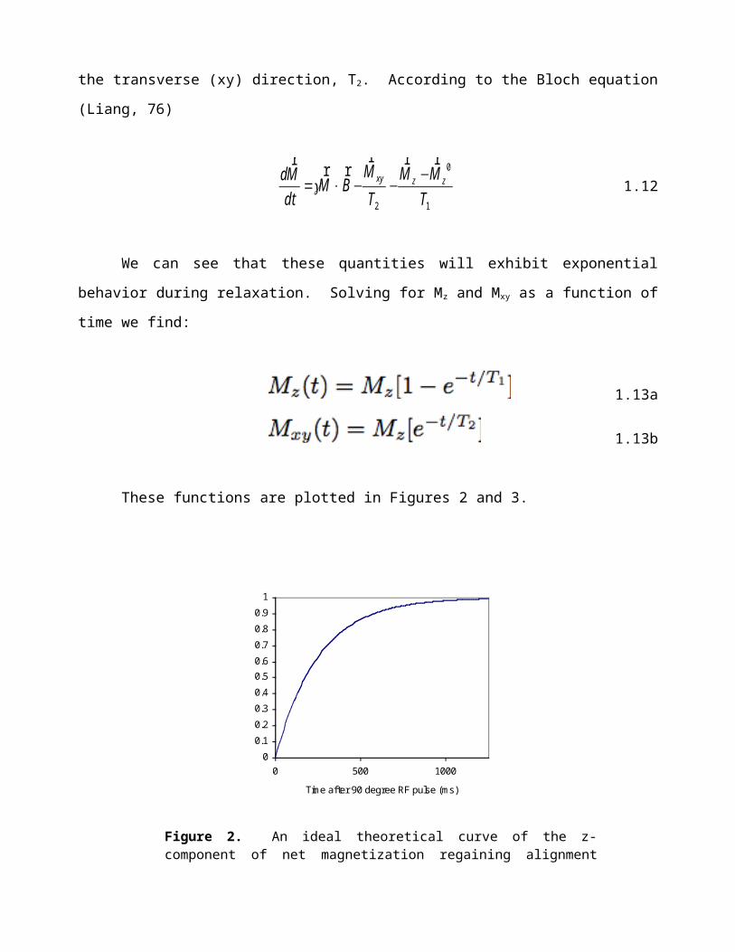
We can see that these quantities will exhibit exponential behavior during relaxation. Solving for Mz and Mxy as a function of time we find:

1.13a

1.13b

These functions are plotted in Figures 2 and 3.

0

0.1

0.2

0.3

0.4

0.50.6

0.7

0.8

0.9

1

0 500 1000

Time after 90 degree RF pulse (ms)

Mz

Figure 2. An ideal theoretical curve of the z-component of net magnetization regaining alignment with the z-axis. The curve corresponds to a T1 time of 250 ms.

0

0.1

0.2

0.3

0.4

0.5

0.6

0.7

0.8

0.9

1

0 100 200 300 400

Time after 90 degree RF pulse (ms)

Mxy

Figure 3. An ideal theoretical curve of the xy-component of net magnetization losing coherence, with a T2 time of 80 ms. In general T1>T2.

The various values of T2 and T1 obtained from tissues are what are used as contrast to produce a visual magnetic resonance image (MRI). The precessing macroscopic bulk magnetization of the NMR subject is responsible for producing the measurable RF signal to obtain the values of T1 and T2.

The final technique this section will address is the use of an “echo sequence”. In any real situation, the magnetic field used in an NMR machine will be slightly inhomogeneous. This implies that the rates of spin precession will vary slightly depending on location. The spins as a whole will therefore quickly become out of phase due to their different rates of precession. The quick decoherence makes obtaining a measurable signal difficult.

To compensate for this effect an additional 180° pulse is applied to “flip” all spin orientations to the other side of the transverse plane. The corresponding spins will then reverse their precession and regain coherence from an “echo” signal. If one imagines a race where all the runners are allowed to run at their own speed, then told to turn back at the same instant, then they will all come back to cross the start line at the same instant, even if the fastest racer covered more ground.

The amplitude A of the echo signal can be shown to be (Liang, 119)

1.14

where the two angles refer to the angles of rotation caused by the first and second pulses respectively.

PROCEDURE:

In this experiment you will measure the values for T2*, T2, and T1 for mineral oil and several samples of water containing varying concentrations of CuSO4. The time constants for pure water are much too long to be conveniently studied with this apparatus, thus the addition of the paramagnetic CuSO4 ions serves as a “relaxation agent”, causing the time constants of the water to shorten. Since we are measuring the signal due to NMR-active nuclei, e.g. single protons, the observed signal is due to the hydrogen found in the mineral oil, and the water in the case of the solutions. After measuring several solutions you will then be asked to identify the concentration of an unknown solution.

To do these experiments, you must first become accustomed to the TeachSpin device. You should read the section titled “The Instrument” in the manufacturer’s literature. You will be applying a RF pulse to a sample in order to misalign the sample’s nuclear dipoles and hence net sample magnetization from a large external magnetic field. You will then “watch” as this magnetization relaxes back into alignment with the large external field. The time that it takes to do this is highly dependent on the material of the sample, and can therefore be used to characterize a sample. Most of the TeachSpin device is fairly straightforward except for the mixer component. The mixer output provides a combined signal from the sample and the oscillator that appears as the envelope of the combined signals. This output will help you determine when the sample is in resonance, e.g. you have chosen the correct frequency for the RF pulse.

You will be searching for the correct way to apply a 180 and later, a 90 (A and B, or α and ) pulse to the sample. As stated above, the 180 pulse will initially rotate the net magnetization of the sample from the equilibrium z direction, thus allowing you to watch its relaxation back to the z-axis. The 90 “echo pulse” then “reverses the race” thereby compensating for the inhomogeneity of the magnetic field. You control both the frequency and width of the pulses. The width of the pulse controls the angle through which the sample’s net magnetization is rotated. The device should be connected as

depicted in Figure 1.3 of in the manufacturer’s literature, and amended with several “T” connectors as depicted below.

QuickTime™ and aTIFF (Uncompressed) decompressor

are needed to see this picture.

Figure 4. The front panel of the TeachSpin Pulsed NMR device. Note the amendments from the manufacturer’s Figure 1.3: “T” connections at “A+B OUT” and “RF OUT.” Although not explicitly necessary, these additional connections will allow you to observe what is happening at these key locations via the oscilloscope.

Observe and estimate pulse values:Before determining the widths of the 90 and 180 pulses for the samples

you should first begin by observing the pulses using the wire probe. The probe provides an explicit way to observe the A and B pulses (rather than the envelopes of the pulses as given by the outputs of the machine) and measure the magnitude of the rotating magnetic field used to rotate the magnetization vector of the sample. The wire probe is encased in plastic and is a simple loop of wire whose surface perpendicular to the plane of the table when inserted into the device. Set the machine to output A pulses only. Connect the wire probe to the oscilloscope, making sure that you are using the appropriate 50 ohm cap by using a T-connector. With the probe inserted, and NMR pulses on, you should rotate the probe and observe a signal on the oscilloscope. The amplitude of this signal depends on the amount of magnetic flux through the loop, from the rotating magnetic field, which is created by using a circularly

polarized wave of radio frequency (RF) waves, and hence on the orientation of the probe. By rotating the probe to obtain the maximum signal amplitude, you have oriented the loop of the probe to be normal to the x-y plane that the magnetic field vector is rotating in. While observing the pulses you should adjust all of the different parameters of the pulse programmer (the middle module) in order to see how they truly change the pulse as seen by the sample.

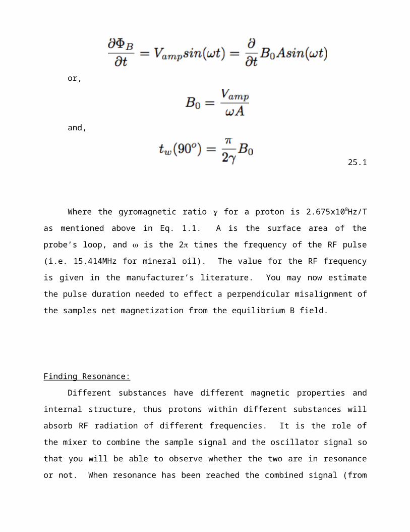
Once maximum amplitude is obtained, a simple application of Faraday’s law allows us to calculate the magnitude of the rotating magnetic field using the amplitude of the voltage trace on the scope. This value is necessary to utilize expression 25.1 (manufacturer’s lit.). Expression 25.1 is important as it allows you to form your first estimate of the duration of a 90 pulse:

or,

and,

25.1

Where the gyromagnetic ratio for a proton is 2.675x108Hz/T as mentioned above in Eq. 1.1. A is the surface area of the probe’s loop, and is the 2 times the frequency of the RF pulse (i.e. 15.414MHz for mineral oil). The value for the RF frequency is given in the manufacturer’s literature. You may now estimate the pulse duration needed to effect a perpendicular misalignment of the samples net magnetization from the equilibrium B field.

Finding Resonance:Different substances have different magnetic properties and internal

structure, thus protons within different substances will absorb RF radiation of different frequencies. It is the role of the mixer to combine the sample signal and the oscillator signal so that you will be able to observe whether the two are in resonance or not. When resonance has been reached the combined signal (from the mixer) will show no beats, and the correct frequency has been chosen for that sample. In order to observe a signal you must first insert a sample. Your first sample should be mineral oil, the clear sample with the yellow cap.

In order for the mixer to work properly, the excitation (pulse) RF must be applied to the mixer constantly in order to be mixed with the sample signal, rather than just during the short pulse interval. In order to do this, flip the continuous RF switch, CW-RF, to ON. This then mixes the RF of the excitation pulse with the actual signal from the sample over a continuous interval. Start by applying an A pulse of width tw (calculated above) and observing the mixer and signal outputs. When the frequencies of the excitation RF and the sample (signal) RF are identical, the mixer outputs no beats, i.e. is an envelope or flat instead of a wave, and resonance is found. Initially one will most likely see a sinusoidal wave coming from the mixer output. The frequency of this wave is the beat frequency between the sample and excitation RF. Adjust the frequency to increase the wavelength of the mixer signal, i.e. approach the condition that the beat frequency is null. You will most likely travel through several near-resonances before true resonance is found. Having found resonance, you may now fine tune the A pulse width to obtain the maximum initial signal amplitude. The decay envelope observed on the signal output is the free induction decay (FID), with time constant T2*. Adjusting the pulse width to obtain maximum signal indicates that we have rotated the magnetization vector of the sample directly into the transverse x-y plane where it is detectable by the machine, or, in other words, in addition to finding resonance, we have applied an exact 90 degree pulse.

The “Sweet Spot”:The manufacturer’s literature discusses finding the “sweet spot” in the

magnetic field. This implies finding the region in which the magnetic field most homogeneous. It is important to the mathematics of NMR that you locate this portion of the magnetic field, as we have used the spinning top analogy to derive many of our relations. The classical top is located in a constant gravitational field, so for the sake of attaining any true physical parallelism and maximum signal quality we must apply a uniform field. Read the section concerning finding the “sweet spot” in the manufacturer’s literature for more information.

You will translate the sample mount carriage in the permanent magnetic field. There will be a location within this field that corresponds to the maximum possible value of T2* i.e. the longest “tail” of the decay envelope, and consequently the most homogeneous field. Be certain to re-maximize the signal at each point however, since changing the location of the sample changes the static B field strength on the sample and thus the resonance frequency. By now you should be comfortable with using the mixer to assure yourself you are at resonance, and maximizing the amplitude of the free induction decay envelope to assure yourself you’ve applied an exact 90 pulse. The logic behind this step is simple: as the field approaches uniformity (over the sample) T2* approaches T2, and maximum signal output is obtained. You will only need to do this once, assuming that you use the same volume of sample in each test tube, and you insert all samples the same distance into the mount.

T2 and T2* of Free Induction Decay:

In this section you will apply your newly created 90 and 180 pulses to obtain useful information about the decay times of different materials. Figure 5 is a mock oscilloscope trace showing all of the components of the pulsed NMR signal and is much cleaner than the actual signal you will observe. The mixer

output on the machine outputs only the envelope of the actual signal and thus hides the fact you are looking at an RF signal as shown in Figure 5. Notice the relation between T2 and T2*. The alpha pulse is the initial 180 pulse, and the beta pulse is the 90 pulse. As you should have noticed while using the wire probe, the time between these two pulses can be varied. This will cause the echo to move underneath the T2 decay function as if the function were an envelope. Theoretically, a 180 pulse is simply twice the length of a 90 pulse, but as you have likely discovered, it is easiest to simply observe the signal, and then apply a B pulse of a width that maximizes your echo amplitude, rather than trying to explicitly measure the width of your pulses.

You will now begin to take data by exporting oscilloscope images directly to the computer (via RS232). You will use a program called Waveform Manager Pro (WFM Pro), which is located in the start menu queue. The interface between the oscilloscope and WFM Pro is enjoyably simple. When you wish to capture data simply toggle the run/stop button (upper right corner) on the oscilloscope. Then press the “capture” button on the WFM Pro toolbar (the butterfly net). This will ask you how you wish to save your file: choose comma separated (.csv). Now you may acquire Channel 1 and Channel 2 by simply clicking the two leftmost buttons on the WFM Pro toolbar. WFM Pro will display the acquired waveform as well as write it to the file that you specified. WFM Pro will also number the files that you capture automatically starting with a 0 amended to the file name you choose. Analyze this data in order to flesh out the exponentials associated with T2 and T2*. Take data for at least 10 different delays between alpha and beta pulses for each sample.

Figure 5. A mock oscilloscope trace showing the relation between T2 and T2*.

Note the echo at twice the delay between the alpha and beta pulses. You will, or course, not see the theoretical signal, but instead enjoy much more noise.

Additional Information, T1:

T1 is the time recovery constant of the sample’s induced magnetization to its equilibrium position (Figure 2). At first, it would seem that T1 and T2 should be trivially related, since a recovery of alignment would correspond to a loss in x-y magnetization. We can’t forget however, that the whole concept of relaxation is a thermodynamic process, and preservation of macroscopic quantities, namely the magnitude of the sample’s magnetic polarization vector, certainly isn’t guaranteed. As it turns out, T1 is as uniquely characteristic to a substance as T2.

In general, T1>T2, but measuring T1 is complicated by the fact that we can’t measure the magnetization along the z-axis with this apparatus. We can only measure magnetization perpendicular to the x-z plane. There is also the problem that Mz does not rotate, and thus produces no RF signal to begin with! The solution is simple. If instead of rotating the initial magnetization of the sample into the x-y plane perpendicular to its equilibrium orientation along z, we just flip the entire vector, from Mz to –Mz. As equilibrium orientation is

regained, this implies the magnitude of –Mz actually decreases (since +Mz is increasing). Since this decrease is only along the z-axis it is simply the decay function associated with T1. We can then apply a 90 pulse to rotate this now decayed |Mz| into the transverse plane for detection. The primitive pulse sequence is as follows:

A(180)--------t-----------B(90)

Following this pulse sequence, the amplitude of the signal directly after the 90 pulse then corresponds to |Mz| after undergoing t length of T1 decay.

REPORT:You should report T2*, T2, and T1 (and their errors, of course) for mineral

oil and each sample of known CuSO4 concentration and for the unknown solution. Based on this information conjecture as to the concentration of the unknown solution. Report the location of the “sweet spot.”

Also, you should consider the following: -What is the magnetic susceptibility of(See Appendix)- What is the magnitude of the magnetic field in the z-direction, |Bz|, at the sweet spot? - What is the ratio of protons aligned to the field to those that are not? ( e -E/kt = e-2BzMz/kt ) - - Are your samples para- or diamagnetic?- Do the glass casings for the samples affect your results?-Magnetic permeability of water …

REFERENCES:

Griffiths, D. Introduction to Electrodynamics. 3rd Ed. Prentice Hall, 1999. pp. 274-5.

Liang, Z. & Lauterbur, P. Principles of Mangetic Resonance Imaging: A Signal Processing Perspective. Wiley-IEEE Press, 1999. pp. 119.

Melissinos & Napolitano. Experiments in Modern Physics. 2nd Ed. Academic Press, 2003. pp. 273-83.

Sakurai, J.J. Modern Quantum Mechanics. Revised Ed. Addison Wesley Longman, 1994. pp. 76.

APPENDIX:

A material can be mathematically labeled para- or diamagnetic depending on its own unique m. See Griffiths (3rd Ed.) page 274. m, the magnetic susceptibility, is a proportionality constant that relates the magnetization of a material M to an applied field H as:

In less exacting lingo, m is the polarizability. By placing the sample within a magnetic field, we induce a magnetic polarization in it, our initial M z. This is the vector that gives us our signal; we rotate it out of z with the excitation pulses of the circularly polarized RF. This magnetization vector is what we are actually measuring/watching via the faraday effect. The signal coils are perpendicular to the x-y plane and thus transmit a signal when the Mz

vector is perturbed. Thus, by knowing the amplitude of B from the RF of part A, the amplitude

of the signal of the pulses via the oscilloscope, and the effective A of the detector, you may quantitatively determine what |M| is by the initial amplitude of an FID after a 90 degree pulse. You can measure Bz with a gaussmeter. Therefore you know |mag|.

As you most likely discovered in Griffiths, mag is positive for paramagnetic materials and

negative for diamagnetic—this cannot be nicely measured by the above procedure to get |M|

because we can’t exactly determine the rotation during the initial pulse, even if we can find |m|.

The previous, easier, complimentary measurement is to use the fact that the total B in a sample is:

where m defines the magnetic permeability of a material (as opposed to the vacuum). You therefore know the resonance for a free proton, as you have measured Bz with a gaussmeter and you can look up the gyromagnetic ratio of a free proton. However, the resonance you find is either above or below the free proton resonance: which tells you both the size AND sign of a m. The problem here though, is that in addition to the macroscopic behavior (which is what m is referring to anyway) the nucleus is also tiny, and it is surrounded by electrons. The electrons impart some magnetic shielding, known as the chemical shift. Does this m even agree in sign with the known negative sign of water’s m?

A third approach is to use thermodynamics. From e-E/kT = e-2BzMz/kT we can determine the ratio of protons aligned against the field to those aligned with. Knowing the density of water, we can also know the density of those dipoles aligned with Bz. Can you verify the negative value of water’s m (-1.2*10-5)?