Embed Size (px)
Citation preview

ISR develops, applies and teaches advanced methodologies of design and analysis to solve complex, hierarchical,heterogeneous and dynamic problems of engineering technology and systems for industry and government.
ISR is a permanent institute of the University of Maryland, within the Glenn L. Martin Institute of Technol-ogy/A. James Clark School of Engineering. It is a National Science Foundation Engineering Research Center.
Web site http://www.isr.umd.edu
I RINSTITUTE FOR SYSTEMS RESEARCH
MASTER'S THESIS
Fixture-Based Design Similarity Measures for Variant Fixture Planning
by Sundar BalasubramanianAdvisor: Jeffrey W. Herrmann
M.S. 99-5

ABSTRACT
Title of Thesis: FIXTURE-BASED DESIGN SIMILARITY MEASURES FORVARIANT FIXTURE PLANNING
Degree candidate: Sundar Balasubramanian
Degree and year: Master of Science, 1999
Thesis directed by: Dr. Jeffrey W. HerrmannDepartment of Mechanical Engineering andInstitute for Systems Research
One of the important activities in process planning is the design of fixtures to position,
locate and secure the workpiece during operations such as machining, assembly and
inspection. The proposed approach for variant fixture planning is an essential part of a
hybrid process planning methodology. The aim is to retrieve, for a new product
design, a useful fixture from a given set of existing designs and their fixtures. Thus,
the variant approach exploits this existing knowledge. However, since calculating
each fixture’s feasibility and then determining the necessary modifications for
infeasible fixtures would require too much effort, the approach searches quickly for
the most promising fixtures based on a surrogate design similarity measure. Then, it
evaluates the definitive usefulness metric for those promising fixtures and identifies
the best one for the new design.

This thesis explores the use of a design similarity measure to find existing designs
that are likely to have useful fixtures. The approach aims to identify design attributes
that reflect the underlying fixture usefulness. Then, it formulates a consistent design
similarity measure that maps the design attributes of a new design and an existing
design to the usefulness of the fixture associated with the existing design for the new
product design. The correlation between the design similarity and fixture usefulness
enables definition of a fixture-based design similarity measure. This approach has
been developed for a class of part designs and modular fixtures. It will enable a
manufacturing firm to reuse dedicated fixtures by identifying an existing fixture that
requires only a minor change to become an effective fixture for a new design. This
will reduce the amount of time spent constructing fixtures. In addition, the variant
procedure requires less computational effort than a generative procedure. It is
economical to have design families based on fixtures, so that a new design can be
assigned to any of these families and changeover times can be reduced. Reusing both
fixtures and fixturing solutions has far-reaching implications in terms of cost and lead
times.

FIXTURE-BASED DESIGN SIMILARITY MEASURES FOR
VARIANT FIXTURE PLANNING
by
Sundar Balasubramanian
Thesis submitted to the Faculty of the Graduate School of theUniversity of Maryland at College Park in partial fulfillment
of the requirements for the degree ofMaster of Science
1999
Advisory Committee:
Dr. Jeffrey W. Herrmann, Chair/AdvisorDr. Satyandra K. GuptaDr. Yu Wang

ii
ACKNOWLEDGMENTS
I would like to express my gratitude to Dr. Jeffrey W. Herrmann for having provided
me with an opportunity to conduct research under his supervision. If I were to be an
advisor someday, he would be my role model. He has had a definitive influence on me
in terms of work organization and written communication. I am thankful to Dr.
Michael Wang and Dr. Satyandra Gupta for having helped me with their comments
and suggestions on different occasions, and for having readily accepted to be a
member of my thesis examining committee. I would also like to thank Dr. Edward Lin
for having helped me in trouble shooting on all those afternoons! I would be making
this thesis bulky (or bulkier?), if I were to mention all my friends who have been part
of my life, in different ways, at Maryland. So, thanks each one of those who have
made the last couple of years at Maryland memorable.

iii
TABLE OF CONTENTS
List of Tables v
List of Figures vi
1. Introduction 1
2. Background 52.1 Process Planning Approaches………………………………………………..6
2.1.1 Introduction…………………………………………………………..62.1.2 Generative Process Planning………………………………………....72.1.3 Variant Process Planning………………………….………………… 72.1.4 Hybrid Process Planning……………………………………………10
2.2 Classification of Fixture Design Research……………………..…………...122.2.1 Introduction…………………………………………………………122.2.2 Fixture-design Principles…………………………………………... 16
General requirements of fixture…………………………….............16Types of location……………………………………………..……..16The 3-2-1 method of location……………………………………... .17
2.3 General guidelines/rules……………………………………………..……...192.4 Fixture Hardware………………………………………………….……….. 21
2.4.1 Basic Components…………………………………………………. 212.4.2 Classification Schemes………………………………………….…. 232.4.3 Modular Fixturing Systems…………………………………..……. 242.4.4 Advanced Fixture-Hardware Design………………………….…… 25
2.5 Summary…………………………………………………………………... 26
3. Generative Planar Fixture Synthesis 273.1 Background………………………………………………………..………..273.2 The 3L/1C Model………………………………………………….………. 293.3 The Complete Algorithm………………………………………….….……. 32
3.3.1 Introduction………………………………………………….…….. 323.3.2 Grow Part…………………………………………………….……. 333.3.3 Enumerate Locator Triplets…………………………………..……. 343.3.4 Identify Part Configurations………………………………..……….363.3.5 Enumerate Clamp Positions………………………………..……….373.3.6 Filter Candidates…………………………………………….……... 393.3.7 Rank Survivors………………………………………………..…….393.3.8 Algorithm Complexity………………………………………..…….403.3.9 Limitations and Extensions…………………………………..……..41

iv
3.4 Summary…………………………………………………..………..………42
4. Variant Fixture Planning Methodology 434.1 A Variant Fixture Planning Approach........................................................... 44
4.1.1 Motivation………………………………………………………… 444.1.2 Description of the Methodology………………………………….. 46
The Algorithm…………………………………………………….. 474.2 Single Attribute Design Similarity Measures……………………………… 51
Maximum Inter-Vertex Distance (MID)…………………………................51Total Enveloped Area (TEA)…………………………………….................51Maximum Vertex-Edge Distance (MVED)………………………...............51
4.3 Neural Network-based Design Similarity Measure………………………... 544.3.1 Introduction………………………………………………………. 544.3.2 Neural Network Architecture…………………………………….. 554.3.3 Classification of Neural Network Models………………………… 584.3.4 Multi-layered Networks………………………………………….. 594.3.5 Three-layered Feed-forward Network……………………………. 594.3.6 The Back-Propagation Algorithm………………………………… 61
Back-Propagation in a Three-layered Feed-forward Network……...61Back-Propagation in a Four-layered Feed-forward Network…….. ..64The Algorithm [Lip87]……………………………………………. .64
4.3.7 Pre-processing……………………………………………………. 65Standardization……………………………………………………. .67
4.3.8 Weight Initialization……………………………………………… 684.3.9 Adaptive Learning………………………………………………… 694.3.10 Cross-Validation………………………………………………….. 704.3.11 Implementation Results…………………………………………… 70
4.4 Comparison of Design Similarity Measures………………………………..734.5 A Complete Example……………………………………………………….754.6 Order of Complexity......................................................................................814.7 Summary……………………………………………………………………81
5. Conclusions and Future Work 835.1 Anticipated Impact………………………………………………………….845.2 Avenues for Future Work………………………………………………….. 85
Bibliography 87

v
LIST OF TABLES
4.1 Network performance (MAD) versus network structure 72
4.2 Correlation coefficients for various design similarity measures 73
4.3 Performance of the different design similarity measures in identifying
the best existing fixture 74

vi
LIST OF FIGURES
2.1 Twelve degrees of freedom for a workpiece 18
2.2 The 3-2-1 method of location 73
3.1 A FixtureNet example 31
3.2 Algorithm for planar fixture synthesis 32
3.3 Growing the part boundary 33
3.4 Clipping of self-intersecting grown edges 34
3.5 (x, y, θ) configuration for a part with respect to a locator triplet 35
3.6 Force sphere analysis 38
4.1 The variant fixture planning algorithm 48
4.2 Ratio of MIDs versus Relative Usefulness Metric 52
4.3 Ratio of TEAs versus Relative Usefulness Metric 52
4.4 Ratio of MVEDs versus Relative Usefulness Metric 53
4.5 A three-layered feed-forward network 60
4.6 A Schematic of the Back-Propagation Algorithm 66
4.7 Oscillations are observed when ε′ = 0.5 for a three-layered network
with seven nodes in the hidden layer 71
4.8 2D projection of a new part input to the variant fixture planner 76
4.9 List of existing designs sorted by their design similarity measures 78
4.10 The new part in the locator triplet from the best existing fixture
identified using the design similarity measure 79
4.11 The new part with its best generatively designed fixture 80

1
Chapter 1
Introduction
Developing successful generative process planners for complex machined parts is a
difficult challenge. Although researchers have developed generative techniques for
process selection, they have been less successful developing generative techniques for
selecting the fixtures needed to complete the process plan. In most cases, a generative
planner is an effective approach for creating a preliminary process plan. A variant
approach is a very useful technique, however, for completing the process plan and
adding the fixturing details.
A process plan describes the steps necessary to manufacture a product. When
done manually, process planning is a subjective and time-consuming procedure, and it
requires extensive manufacturing knowledge about manufacturing capabilities, tools,
fixtures, materials, costs, and machine availability. In addition, the process planner
must carefully document the plan using standard notation and forms. Computer-aided
process planning (CAPP) software systems automate many functions, which reduces
the chance of error, and the process planner can work more quickly.

2
In machining and other types of operations such as inspection and assembly, an
important part of process planning is fixture planning - determining the fixture that
holds a workpiece firmly in position in a particular setup and provides a means to
reference and align the cutting tool or probe to the workpiece. Proper location of the
workpiece is essential to ensure accuracy and repeatability of the machining process
[Hof84].
Fixture planning is an important issue in small-batch manufacturing, which
requires the flexibility of modular fixtures. While many areas have been explored to
improve the cost-effectiveness of a manufacturing activity, none have as dramatic an
impact on productivity as workholding practice [Hof87]. Like process planning in
general, identifying a good fixture for a given operation is a difficult task. Fixture
planning is difficult because there are many different types of fixtures and fixture
elements, and the fixture has to satisfy many constraints on stability, location,
restraint, accessibility, and cost.
Although fixturing contributes significantly to overall manufacturing cost, it is
sometimes neglected for the reason of cost reduction. Fixturing contributes
significantly to the overall manufacturing cost. The typical cost of dedicated fixtures
ranges from ten to twenty percent of the total manufacturing cost [Gan86].
Fixtures that are specially designed and built for a particular workpiece are called
dedicated fixtures. They achieve quick positioning and clamping at the expense of
high tooling cost. However, the trend is towards more flexible, modular fixturing
systems that promote a larger product mix, flexibility, and quality. A modular fixture

3
system includes baseplates that have a lattice of holes for mounting locators and
clamps precisely. A modular fixture system is flexible because one can construct a
large number of fixture configurations from different combinations of standard fixture
elements. Hence, lead times are shorter, engineering changes are easier to handle, and
storage costs are reduced.
This thesis describes a variant fixture planning approach that uses a design
similarity measure to identify promising fixtures. The goal is to retrieve, for a new
product design, a useful fixture from a given set of existing designs and their fixtures.
However, since calculating each existing fixture’s feasibility and then determining the
necessary modifications for infeasible fixtures would require too much effort, the
approach uses a fixture-based design similarity measure to find existing designs that
are likely to have useful fixtures. All existing designs are paired against the new
design to evaluate a similarity measure at the design level. For each promising fixture,
the approach calculates a precise usefulness metric that describes how well the
existing fixture can hold the new design.
The variant fixture planning approach described in this thesis is part of a hybrid
process planning methodology. The hybrid process planning approach extends the
generative approach that Gupta et al. [Gup94] describe. After using that approach for
process selection, it employs a variant procedure to select fixtures, which completes
the process plan. For more details, see Section 2.1.4.
This approach has been developed for a class of part designs and modular fixtures.
It will enable a manufacturing firm to reuse dedicated fixtures by identifying an

4
existing fixture that requires only a minor change to become an effective fixture for a
new design. This will reduce the amount of time spent constructing fixtures.
The benefits of reusing existing fixtures are more significant for dedicated fixtures
than for modular fixtures since modifying a dedicated fixture requires more effort.
However, the variant fixture planning methodology has been implemented in the
modular fixture to demonstrate the feasibility of our approach.
The remainder of the thesis is organized as follows: Chapter 2 presents a
background for hybrid process planning and describes related research in automated
fixture design. A classification of issues in fixture design is presented, including an
overview of fixture design principles, and fixture hardware design, with emphasis on
modular fixture systems. A hybrid variant-generative process planning approach is
also described in this chapter, which includes an overview of generative and variant
approaches to process planning and fixture selection.
Chapter 3 describes a generative planar fixture synthesis system called FixtureNet
(developed by Richard Wagner, Ken Goldberg, Xiaofei Huang and Randy Brost
[Bro96]). The variant planar fixture planning system described in this thesis reuses
some of these routines for designing modular fixtures. Chapter 4 presents a design
similarity approach to variant fixture selection and proposes various design similarity
measures and associated results that illustrate the correlation between the similarity
measures and usefulness metrics. Chapter 5 describes the contributions of this work,
research issues not addressed in this thesis and avenues for future work.

5
Chapter 2
Background
This chapter presents a review of literature and current developments in computer-
aided fixture design and past work in hybrid process planning and fixture planning.
The chapter outlines the motivation for growing research in computer-aided fixture
design, primary factors being reduction in setup and production times and hence,
reduction in the associated costs. The review addresses both the micro aspects such as
fixture design verification and the macro aspects of fixture design such as the
integration with other computer-aided tools in manufacturing.
Section 2.1 describes various process planning approaches. This section presents a
review of traditional variant and generative approaches to process planning, and
efforts at combining these two traditional approaches to overcome their associated
drawbacks. This section also delves into some of the generative fixture design systems
and reviews efforts towards a variant approach to fixture selection. Section 2.2
classifies fixture design research, current developments in automated fixture design
and discusses the principles of fixturing. Section 2.3 presents some empirical design
rules that govern some of the current automated fixturing systems. Section 2.4

6
describes different fixture systems currently in use, and includes a description of
modular fixture systems and their increasing popularity in job shop environments.
Section 2.5 summarizes the literature in automated fixture design and describes the
relevance of the work presented in this thesis.
2.1 Process Planning Approaches
2.1.1 Introduction
A process plan describes the manufacturing steps necessary to create the physical
embodiment of a product, with its desired engineering specifications, such as
tolerances. A process planner has to consider the capabilities of the manufacturing
facility in terms of labor, machine, production quantity, lead time and due date. Hence,
when done manually, process planning is a subjective and time-consuming procedure,
and it requires extensive manufacturing knowledge about manufacturing capabilities,
tools, fixtures, materials, costs, and machine availability.
The process planner must carefully document the plan using standard notation and
forms. This problem is more acute in a job shop environment where the total time
available for process planning is much less than in a repetitive manufacturing
environment. Additionally, complexity of the planning activity is much greater in a
job shop environment. Notwithstanding commercially available CAPP systems, there
is a reluctance on the part of manufacturers to rely on these computer-aided systems.
Different segments of the manufacturing community define process plan in different
ways, leading to ambiguity in the description of a process plan.

7
2.1.2 Generative Process Planning
Generative Process Planning systems attempt to synthesize a process plan directly for
a given design. A typical generative process planning system for machining is
described as follows:
• Extract the manufacturing features in given product design.
• Using the manufacturing knowledge base, and heuristics to generate candidate
process plans for each of the identified manufacturing features.
• From these candidate process plans, develop an optimal process plan that confirms
to the geometric and manufacturing constraints imposed on the product design.
A number of generative systems have been developed for various aspects of
process planning. For a detailed review and pointers for literature on generative
process planning, see [Gup94]. Generative process planning has proved difficult. A
generative process planning system capable of generating realistic process plans for a
wide spectrum of products has not been developed. Most generative process planning
systems work only in restricted domains. Difficulties arise due to interaction with
issues such as process selection and process sequencing. However, generative process
planning can be useful in Design for Manufacturing (DFM), in which the designer
tries to take manufacturability considerations into account during the design stage.
2.1.3 Variant Process Planning
The variant process planning technique was one of the first approaches to be used in
computerised process planning. Variant process planning systems exploit the
hypothesis that similar designs will have similar process plans. They use the similarity

8
among components to retrieve existing process plans. The variant process planner
provides a standard plan for the product family that the new design belongs to and this
plan can be further modified to meet specific geometric and manufacturing
requirements of the new design.
In general, variant process-planning systems have two operational stages [Cha98]:
• Preparatory Stage: Existing designs are coded, classified, and grouped into
families. The selection of a coding system that covers the entire spectrum of parts
produced in the shop is important. Once family matrices for each family are
formed, standard process plans for the part families are prepared. Subsequent to
preparatory stage, the system is ready to use.
• Production Stage: A new design is first coded. The family to which the new design
belongs is identified. The standard plan associated with this family is retrieved and
necessary modifications are incorporated.
Several variant process planning systems are commercially available. Some of
them are MIPLAN, MITURN and MAYCAPP. Group Technology (GT) codes have
become the de facto standard for design classification in a variant approach. However,
other techniques ([Her97], [Sin97]) based on design similarity measures, that are
independent of part family formation, have been proposed.
Typically, variant process planning systems involve the following steps:
• The Group Technology (GT) based coding scheme is used to map a design D into
an alphanumeric code.

9
• This code is then used to search a database that contains designs and their
corresponding process plans. A process plan P0 for a design family F0 that the new
design D belongs to or the process plan P0 for a design D0 similar to D is retrieved.
• Then the retrieved process plan P0 is modified manually to produce process plan P
that would meet the specific requirements of the design D.
The advantages of variant process planning are:
• The total time required to generate a complete process plan for a new design is
reduced considerably because the planning task is limited to modifying a retrieved
plan.
• The planner does not have to explain his selection of process specifications, since
it would already have been accounted for when the plans in the database were
created.
• Generating and evaluating alternate process plans is facilitated and this leads to a
more realistic process plan for the new design.
Some of the disadvantages behind the variant process planning approach are:
• For a first-of-its-kind or a unique design, this approach will fail and the planner
would have to resort to generative process planning.
• If the process plans in the design repository have outdated processes or practices,
the process plan obtained from a variant approach may become ineffective.
Problems in old plans will propagate to new ones.

10
• This approach will prove inappropriate if the production quantities vary
significantly, since the retrieved process plans would then have inappropriate
processes.
2.1.4 Hybrid Process Planning
A hybrid process planning approach combines the best characteristics of both variant
and generative process planning while avoiding their worst limitations. A hybrid
process planning approach exploits knowledge in existing plans while generating a
new plan. See [Sin97] for a review of literature on hybrid process planning.
Previous research was towards a subplan completion approach. The method finds
subplans for each portion of the design and then combine and modifies these subplans
[Mar94], [Eli97]. An alternative is the plan completion approach where the generative
planner identifies and sequences the manufacturing processes, while the variant fixture
planner completes the plan. This hybrid process planning approach extends the
generative approach that Gupta et al. [Gup94] describe.
In a machining operation, a cutting tool is swept along a trajectory, and material is
removed by the motion of the tool relative to the current workpiece. The volume
resulting from a machining operation is called a machining feature. A machining
feature corresponds to a single machining operation made on one machine setup. Each
machining feature has a single approach direction (or orientation) for the tool. Features
are parameterized solids that correspond to various types of machining operations on a
3-axis machining center: side-milling, face-milling, end-milling, and drilling. A
design is represented as a collection of machining features.

11
Given this feature-based representation, there may be, in general, several
alternative representations of the design as different collections of machinable
features, corresponding to different ways to machine the part. The generative approach
proceeds as follows:
Repeat the following steps until every promising feature-based model (FBM) has
been examined:
• Generate a promising FBM from the feature set. An FBM is a set of machining
features that contains no redundant features and is sufficient to create the part. An
FBM is unpromising if it is not expected to result in any operation plans better
than the ones which has already been examined.
• Do the following steps repeatedly, until every promising operation plan resulting
from the particular FBM has been examined.
• Generate a promising operation plan for the FBM. This operation plan represents a
partially ordered set of machining operations. We consider an operation plan to be
unpromising if it violates any common machining practices.
• Estimate the achievable machining accuracy of the operation plan. If the operation
plan cannot produce the required design tolerances and surface finishes, then
discard it. Otherwise, estimate the production time and cost associated with
operation plan.
• For each setup in the operation plan, design a fixture in the following way: Search
a database of existing designs, process plans, and fixtures, for promising fixtures
that could be used for the new design. Verify their feasibility and identify the best
one for the new design.

12
• If no promising operation plans were found, then exit with failure. Otherwise exit
with success, returning the operation plan that represents the best tradeoff among
quality, cost, and time.
This thesis addresses the variant fixture planning portion of this hybrid process
planning approach. An introduction to research in variant fixture planning is presented
in Section 2.2.1. Chapter 4 addresses the proposed variant fixture planning
methodology in detail.
2.2 Classification of Fixture Design Research
2.2.1 Introduction
The function of a jig or fixture is to locate and hold a workpiece firmly in position
during a manufacturing process. Locating denotes attaining the required positional and
orientational relationship between the workpiece and any processing equipment, such
as a machine tool. Holding (clamping) relates to maintaining the workpiece in the
required position and orientation. Additionally, fixtures might also provide support to
workpieces with insufficient stiffness to prevent deformation.
Fixture planning is an intuitive process, traditionally regarded as a manual process
due to requirements of extensive heuristic knowledge and was entirely based on the
discretion and experience of the tool designer. The design and manufacture of fixtures
can be time consuming, and it increases the manufacturing cycle time of any product
that needs operations such as machining, inspection or assembly [Har94].

13
Early research in fixturing began in the 1940’s. This led to the development of
manuals and guidelines for jig and fixture design. Interest in research on computer-
aided planning of fixtures has been growing in recent years. Emphasis has been
towards eliminating human intervention and increasing automation. There is a vast
body of literature in the overall automation of fixture configuration and assembly.
There also have been efforts towards fixture design automation for specified
application domains (such as, automated fixture design for assembly).
Research in fixture configuration has been concentrated primarily in two areas
([Cha92], [Tra90]):
• Search of a mathematical solution for locating and holding a part.
Research in this category involved fundamental analysis of the existence of
fixtures, fixture analysis and fixture synthesis. The objective is to find a mathematical
fixturing solution so that a part is constrained kinematically by means of a set of
contacts. In other words, determine this set of contacts that are able to resist arbitrary
forces and torques on the part. This can be analyzed using the concept of a wrench,
which is a generalized force that includes moment contributions.
Asada and By [Asa85] introduced the concept of automatically reconfigured
fixturing (ARF) for advanced flexible assembly. They developed analytical tools
through the kinematic modeling, analysis, and characterization of workpart fixturing
that determine whether a given fixture design provides total constraint of a rigid body.
They derived conditions for attaining deterministic positioning and the total constraint
of the workpiece for assembly operations and these conditions play a central role in

14
calculating possible positions for point-type fixture components (or fixels) for a given
part.
Extending this analysis, Brost and Goldberg ([Bro96], [Zhu96]) developed a
complete algorithm for automatic design of planar fixtures (described in detail in
Chapter 3) using modular components. Nguyen [Ngu88] proposed an algorithm for
fixture synthesis where a set of four independent regions on the boundary of a polygon
can be identified such that a frictionless contact applied to each region can provide
form closure (total constraint). These issues are discussed in detail in Chapter 3.
Similarly, it is known that seven wrenches are necessary to obtain form closure for 3D
objects.
• Reduce fixture planning into computer routines.
Optimal or applicable solutions from all possible choices for each fixture
component are determined and the fixture components are assembled into the required
fixture. Fixture planning with rule-based expert systems gained significant attention.
Darvishi and Gill [Dar90] developed a fixture design expert system (FDES) which is
based on examining the design goals to be achieved and then creating rules to satisfy
these imposed specifications. For other knowledge-based routines developed, see
[Cho94], [Dar90], [Gan86], [Nna89], [Fer88], [Fuh93], [Yue94], [Sen92], and
[Nee91]. Other approaches include expert systems to determine fixture setups by
considering tolerance requirements [Boe88] and reconfigurable fixture modules for
robotic assembly [Shi93].

15
Similar to computer-aided process planning, there are two approaches to fixture
design: generative and variant. While all the existing fixture design systems described
so far in this section have been generative fixture design systems, there has been
considerably lesser concentration in the area of variant fixture design.
Nee et al. [Nee92] propose a variant fixture design system based on a feature-
based classification scheme for fixtures. A workpiece belonging to the same part
family is assumed to have similar machining features and/or requiring similar
operation sequences and setups. Lin et al. [Lin97] combined the pattern recognition
capability of neural networks and the concept of Group Technology (GT) to group
workpieces with different patterns but identical fixture modes into the same group.
After training the network, any given new workpiece can be classified into a particular
fixture mode and the selection of fixture components can be completed. Senthil Kumar
et al. [Sen95] adopted a Case-Based Reasoning (CBR) technique for automatic
retrieval of fixture designs and modifications to suit the requirements of the new
workpiece. For each setup, suitable fixture-cases from the case-base are retrieved and
modified using the design strategies. Note that the first two techniques are based on
part family formation in the preparatory stage, where existing designs are classified
into families. On the other hand, the CBR technique does not involve part family
formation. This thesis proposes a methodology that is also independent of part family
formation in the preparatory stage. However the design similarity approach to variant
fixture planning described in this thesis can be used to dynamically form fixture-based
design families, as proposed in Chapter 5.

16
2.2.2 Fixture-design Principles
The fundamental principles of basic fixture design and the basic requirements of a
fixture are reviewed in this section. The basic requirement of a fixture is to locate and
secure the workpiece in the required position and orientation, to assure repeatability.
The primary components of a typical fixture include locators, clamps and supporters.
Locators help in positioning the workpiece in static equilibrium. Clamps hold the
workpiece firmly against the locators for rigidity. Supporters provide additional
support to reinforce the stability of the workpiece.
General requirements of fixture
There are four general requirements of a fixture [Har94]:
• Accurate location: A fixture must locate the part accurately with respect to the
machine coordinate system and the workpiece coordinate system. If locating error
is too large, a different locating surface must be chosen.
• Total restraint: The fixture must hold and restrain the workpiece from external
forces, for example, cutting forces.
• Limited deformation: Under the action of clamping forces and cutting forces, a
workpiece may deform elastically or plastically. In such cases, additional supports
can be provided.
• No machine interference: There should be no interference between the fixture
components and the environment in which the workpiece is processed.
Types of location
There are four types of location [Hof84]:

17
• Plane location – Plane location normally refers to locating a flat surface with
reference to a particular surface. However, irregular surfaces may also be located
with this method.
• Concentric location – It refers to locating a workpiece from an internal or external
diameter.
• Radial location – It normally supplements concentric location. The workpiece is
first located concentrically and then a specific point on the workpiece is located to
provide a fixed relationship to the concentric locator.
• Combined location – A combination of the above methods to completely locate a
workpiece, when any of the above methods cannot provide deterministic location
on their own.
The 3-2-1 method of location
Common locating rules in practice are the 3-2-1 or the 4-2-1 methods for clamping.
These rules provide the maximum rigidity with the minimum number of fixture
components. A workpiece is free to move either of two opposed directions along three
mutually perpendicular axes, and may rotate in either of two opposed directions
around each axis, clockwise and counterclockwise. Each direction of movement is
considered one degree of freedom. Hence the workpiece has a total of twelve degrees
of freedom, as shown in Figure 2.1. A workpiece may be positively located by means
of six points positioned so that they restrict nine degrees of freedom of the workpiece.
This is the 3-2-1 method of location (an equivalent method is the flat-2-1 support,
where the primary locating surface is a flat surface), as shown in Figure 2.2.

18
When through-holes are to be machined in a setup, flat-2-1 method of location is
ineffective, and either 3-2-1 or 4-2-1 method is adopted. In the 4-2-1 method of
location, four points are positioned on the primary locating surface.
Figure 2.1. Twelve degrees of freedom for a workpiece
x axis
z axis
y axis
9
67 10
1
2
12
3
4
5
11
8
Figure 2.2. The 3-2-1 method of location
X
Z
Y
P12
P13P11
Three locators positioned onthe first datum plane called the
Primary Locating Surface
P22P21
Two locators positioned onthe second datum plane
called the SecondaryLocating Surface
P31One locator positioned on
the third datum planecalled the TertiaryLocating Surface

19
2.3 General guidelines/rules
As mentioned earlier, most rule-based or knowledge-based expert systems attempt to
capture the heuristic knowledge and craftsmanship of a tool designer in the form of
guidelines or rules. A number of rules have been formulated to identify the locating
and clamping surfaces on a workpiece. The following are some rules that play a role in
these rule-based fixture design systems:
• When clamping a part, the cutting forces should always be used to aid in holding
the part.
• Forces exerted by the clamps must always be directed toward a support or locator.
If a clamp must be positioned in an unsupported area of the part, a supplementary
support should be installed to prevent distortion.
• Clamps should be positioned on surfaces that are rigid before and after machining.
Clamping over an area, which is to be machined to a very thin wall thickness,
could cause the part to warp or deform.
• If surface milling is scheduled in that setup, then clamping has to be done from the
sides of the part.
• If there are through-holes on the supporting face that require machining in that
setup, then the part must be elevated to avoid collision of the tool with the base
plate.
• The size of a locating face should be greater than the diameter or width of the
locating element.
• The height of the locating element should not be greater than the height of the part,
to avoid collision with the tool.

20
• Parts of the same geometric design but with different tolerance specifications
usually require distinct processing steps and sequences; hence, have different
locating and holding requirements for fixturing.
• The closer the fixture component is placed to a machined feature, the more the
machining operation is restricted.
• A process plan has to be designed not only to produce the geometric features of the
designed part but also to machine the locating surfaces (if required).
• The planning and design of a fixture are influenced to a great extent by the number
of parts to be produced.
• The selection of the primary locating surface cannot simply be based on part
geometry. The configuration of the machine tool and the positional and
orientational tolerances of the geometric features to be machined are important
considerations.
• The spatial orientation of the part cannot be completely determined by the primary
locating surface; it is further defined by the secondary locating surface.
• The tertiary locating surface is only to determine the position of the part along the
spatial orientation defined by the primary and the secondary locating surfaces; it
serves only as a stop for repetitive and accurate positioning.
• A fixture component is selected primarily based on the following factors:
� Form of the part surface to be supported, workpiece geometry.
� Dimensional ratio of the part surface to the surface of the fixture component.
� Degrees of freedom to be limited.

21
• Other factors that influence fixture unit selection are – support of workpieces with
insufficient stiffness, balancing of the centrifugal force in the case of turning
operations, easy removal of chips by coolant flow, and convenient access of tool.
2.4 Fixture Hardware
2.4.1 Basic Components• Mounting Components – Mounting blocks are a form of locating and supporting
elements that are used to position locators and clamping devices at specific heights
off the mounting base. E.g. Base Plates, Angle Plates, Mounting or Riser Blocks,
Sine Table and Rotary Table Bases.
• Locating Units – External and Internal Locators.
• External Locators – Devices which are used to locate a part by its external
surfaces. There are two categories – Fixed and Adjustable.
Fixed external locators are solid locators that establish a fixed position for the
workpiece. Some instances of fixed locators are:
• Integral Locators – These locators are machined into the body of the work holder.
Hence, it requires added time to machine the locator, and additional material has to
be provided to allow for machining of the locator.
• Locating Pins – These are the simplest and most basic form of locating element.
• V-Locators.
• Locating Nests – These locators involve a cavity in the work-holder into which the
work-piece is placed and located. No supplementary locating devices are required.

22
• Edge Bars and Edge Blocks.
Adjustable external locators are movable locators that are frequently used for
rough cast parts or similar parts with surface irregularities. Some instances of
adjustable locators are:
• Threaded Locators.
• Spring Pressure Locators.
• Equalizing Locators.
• Internal Locators – Here, locating features, such as holes or bored diameters, are
used to locate a part by its internal surfaces. There are two categories: Fixed and
Compensating.
� Fixed – These locators are made to a specific size to suit a certain hole
diameter. E.g. Machined locators, Pin locators.
� Compensating – These are generally used to centralize the location of a part or
to allow for larger variations in hole sizes. Two typical forms are conical and
self-adjusting locators.
• Clamping Units – Toe-Clamps, Strap Clamps, Screw Clamps, Cam Clamps,
Wedge-Action Clamps, Toggle Clamps, Swing Clamps, Hook Clamps.
• Locating and Clamping Units – Vises, Collets, Chucks, Indexing Units.
2.4.2 Classification Schemes
Fixtures can be classified based on the type of operation to be performed on the part.

23
• First Operation Fixtures – fixtures that are used to hold the part for an initial
machining operation. These fixtures are more difficult to design due to the typical
lack of adequate reference or locating surfaces.
• Second Operation Fixtures – fixtures that are used to hold and locate the part for
any subsequent machining operations. These fixtures are relatively easier to design
since locating surfaces are usually already available.
Modular fixturing systems can be classified into the following categories:
• Sub-plate system.
• T-slot system.
• Dowel pin system.
Fixtures can also be classified based on the associated machine tool with which
they are designed to be used:
• Milling fixtures - The following are some guidelines for milling fixture design:
� Whenever possible, the tool should be changed to suit the part. Moving the part
to accommodate one cutter for several operations is not as accurate or as
efficient as changing cutters.
� Locators must be designed to resist all tool forces and thrusts. Clamps should
not be used to resist tool forces.
� Milling fixtures should be designed and built with a low profile to prevent
unnecessary twisting or springing while in operation.

24
� The entire workpiece must be located within the area of support of the fixture.
In those cases where this is either impossible or impractical, additional
supports must be provided.
� Clearance space or sufficient room must be allotted to provide adequate space
to change cutters or to load and unload the part.
• Lathe fixtures - The following are some guidelines for lathe fixture design:
� Since lathe fixtures are designed to rotate, they should be as lightweight a
possible.
� Lathe fixtures must be balanced, especially at high rotational speeds.
� Projections and sharp corners should be avoided since these areas will become
almost invisible as the tool rotates and could cause serious injury.
� Parts to be fixtured should, whenever possible, be gripped by their largest
diameter, or cross-section.
2.4.3 Modular Fixturing Systems
Fixtures that are specially designed and built for a particular workpiece are called
dedicated fixtures. They achieve quick positioning and clamping at the expense of
high tooling cost. The fixture components are usually welded together, hardened and
ground. This ensures repeatability and facilitates loading and unloading, and meeting
stringent design specifications. However, the need for flexibility and the increasing
design complexity necessitate flexible fixturing systems such as modular fixtures.
Additionally, smaller batch sizes in production, and the greater usage of multiple axis
CNC machine tools [Har94]. The trend is towards more flexible, interchangeable,

25
modular fixturing systems that promote a larger product mix, flexibility, and quality.
Modular fixturing systems achieve flexibility through multipurpose fixturing elements.
A modular fixture system includes baseplates that have a lattice of holes for
mounting locators and clamps precisely. A modular fixture system is flexible because
one can construct a large number of fixture configurations from different combinations
of standard fixture elements. Modular fixtures reduce the need for storage space
compared to dedicated fixtures. They also reduce the time and labor cost in designing
fixtures. Hence, lead times are shorter, engineering changes are easier to handle, and
storage costs are reduced. Modular fixturing elements are manufactured with high
tolerances and the total cost of a modular fixturing kit can be amortized over the entire
production volume.
There are three broad categories of modular fixturing systems [Hof87]:
• T-slot – E.g. Erwin Halder Modular Jig and Fixture System, USA.
• Grid hole – E.g. Yuasa Modular Flex System, USA.
• Dowel pin – E.g. Bluco Technik, Germany.
The major disadvantage of modular fixtures is the issue of tolerance stackup with
the assembly of standard components. Hence, manufacturers attempt to reduce
inadequacies by hardening and grounding fixture elements.
2.4.4 Advanced Fixture-Hardware Design
This section describes other ideas for advanced fixturing hardware that have been
developed. Efforts have been towards automating fixture assembly with robot

26
manipulators, electronic sensors or hydraulic devices to control the fixturing process,
or computer-controlled fixturing process.
Gandhi and Thompson [Gan86] developed a two-phased fluidized bed as a phase-
changing fixturing system to conform to workpieces with complex features.
Reconfigurable [Shi93] and robot-loadable modular fixtures [Asa85] have been
studied extensively in the recent years, in particular, for sheet-metal drilling and
electronic-appliance assembly. However, modular fixtures are the only commercially
available fixturing systems, at the moment.
2.5 Summary
Most of the research in variant fixture design has concentrated on knowledge based
systems using alphanumeric GT codes to group designs and code fixtures and
workpieces. However, a variant fixture design system that involve mathematical
analyses are absent. While numerous generative fixture designs have been developed
involving mathematical techniques to determine the existence of fixtures, fixture
analysis and fixture synthesis, variant fixture design systems in this realm of fixture
planning are few. This thesis specifically addresses this issue, where the attempt is to
reduce the computational effort involved in arriving at mathematical solutions for
fixture designs, without compromising on the adequacy of the approach to provide
satisfactory fixture designs, if not optimal.

27
Chapter 3
Generative Planar Fixture Synthesis
Research in fixture automation was classified and summarized in Chapter 2. Previous
efforts in the area of fixture synthesis in the form of a mathematical solution for
locating and holding a part were listed. This chapter describes one such generative
fixture synthesis methodology, developed by Brost and Goldberg [Bro96], that forms
the basis for the variant fixture planning framework described in Chapter 4. Section
3.1 provides an introduction to the existence of modular fixturing solutions for
polygonal parts and the algorithm for planar fixture synthesis. Section 3.2 describes
the 3L/1C model that the fixture synthesis algorithm addresses. Section 3.3 describes
the algorithm in detail, highlighting some of the key issues involved in computing a
mathematical fixturing solution. Section 3.4 presents a summary of the algorithm
described in this chapter.
3.1 Background
Modular fixturing systems provide a lattice of holes with precise spacing and a set of
locating and clamping units that can be attached to the lattice. Hence, the fixels

28
(fixture components) are selected from a discrete set of locations. Manual design of
fixtures often involves expertise and can be time consuming. Moreover, the fixtures
designed need not be optimal.
In designing non-modular fixtures, the fixture locations are selected from a
continuum in space, which results in an uncountable set of alternative fixture designs.
By limiting fixel locations to a discrete set of points on a regular lattice structure, we
can reduce the number of alternatives. However, a systematic analysis and
enumeration of possible fixture layouts is required so that the designer does not settle
upon a suboptimal design.
A fixture must provide deterministic positioning. The fixture has to locate the part
in a unique position and orientation. Further, we require that the fixture establish form
closure. A fixture is considered to provide form closure when there exists no
admissible workpiece motion. In other words, the fixture has to provide total
constraint. This condition is required of the final fixture layout when the clamp is
introduced.
The part might include certain regions that must remain free of fixture components
for reasons such as clearance for grasping, assembly, machining and other operations.
These are called geometric access constraints. Hence, an admissible fixture must
confirm to these constraints.
Zhuang et al [Zhu96] demonstrated the existence of modular fixturing
solutions for rectilinear parts. Two classes of fixtures were considered, the 3L/1C (3
Locator/1 Clamp) model and the 4C (4 Clamp) model. It has been shown that the

29
3L/1C class of fixtures is not universal for polygonal parts. In other words, we can
identify a family of parts that are unfixturable with this class of fixtures. For the 4C
model, there always exist fixtures with certain constraints on edge lengths.
Brost and Goldberg [Bro96] developed a complete algorithm for synthesizing
planar (2D) fixtures. The algorithm is based on an efficient enumeration of fixture
designs that exploits part geometry and a force analysis. This algorithm is complete
because it enumerates all admissible fixtures for an arbitrary polygonal part projection.
This algorithm is analogous to the 3-2-1 fixture design principle that was described in
Section 2.2.2.
This algorithm forms the basis for FixtureNet, an online interactive computer aided
fixture design system developed by Richard Wagner, Ken Goldberg, Xiaofei Huang
and Randy Brost. FixtureNet is a model for designing modular fixtures via the World
Wide Web targeted towards use both in the industry and in research. To test the
software, visit http://memento.ieor.berkeley.edu/fixture/. FixtureNet provides the
framework for the variant fixture planner that is described in Chapter 4.
3.2 The 3L/1C Model
The FixtureNet algorithm [Bro96] is limited to a particular class of products and
modular components. One face of the part rests on a supporting plane (a baseplate)
and the fixture elements constrain all motion of the part in the supporting plane. Thus,
only the 2D projection of any given design onto the supporting plane is needed for
fixture planning. Only polygonal shapes are considered. In this setting, a fixture is a

30
set of three round locators and one clamp (generically termed as fixels), providing four
point contacts and does not rely on friction. A locator setup consists of three locator
positions and an associated part configuration where the part is in contact with the
three locators.
Each locator is centered on a lattice point and the clamp has one translational
degree of freedom along the principle directions of the lattice. Thus a clamp is
attached to the lattice at any of the lattice points so that the clamp maintains contact
with the part at a variable distance. For simplicity, all contacts are assumed to be
frictionless (Note that a solution set for zero friction is included in the solution set for
a nonzero case). Hence, the 3L/1C model arrests three degrees of freedom; two along
the principle axes and a rotational degree of freedom about an axis perpendicular to
the supporting plane.
Figure 3.1 shows an example of a part, which is a plastic housing for a glue
gun. The part is represented by a polygon that describes its boundary. The clamp is
represented by its planar boundary that includes the space occupied by the clamp
plunger within its limits. The algorithm provides an optimal solution since it
enumerates all admissible fixture layouts that can be ranked based on a user-specified
quality metric. The metric displayed in Figure 3.1 is user-specified. For a discussion of
quality metrics, see Section 3.3.7.

31
Figure 3.1 A FixtureNet example. Total number of fixturesfound = 1135. Quality metric for best fixture = 46.264

32
3.3 The Complete Algorithm
3.3.1 Introduction
A part or workpiece is represented by its 2D projection (a simple polygon). Locators
are represented by circles. The size of the locators (fixel radius) can be selected by the
user. All contacts are frictionless point constraints and all fixture components may
contact only the interior of any part edge. Fixel contacts with part vertices are avoided
since vertices have high stress concentrations that render them more vulnerable to
deformation. Figure 3.2 presents a schematic of the algorithm. The following sections
describe the constituent stages in the algorithm in detail.
Grow Part
Enumerate Locator Triplets
Identify Part Configurations
Enumerate Clamp Positions
Filter Candidates
Rank Admissible Fixtures
Figure 3.2 Algorithm for planar fixture synthesis

33
3.3.2 Grow Part
Contact between the part edges and the fixels are treated as point contacts. To enable
this, the part is grown by an amount equal to the fixel radius using a Minkowski sum
operation of the polygonal part boundary and the circular fixel shape. Assuming that
the fixel radius is the same for all fixture components and that the fixel radius is not
greater than half of the grid spacing on the lattice (to avoid collision between two
adjacent fixels on the lattice), we transform the input polygon so that we can treat the
round locators and the clamp plunger as points. Thus point contacts are equivalent to
the contact between the original part and the finite-radius fixels.
Note that growing the part results in an expanded part boundary with rounded
edges corresponding to the vertices in the original part boundary. Figure 3.3 illustrates
the growing of a part along with the circular fixel boundary. However, we need to
Figure 3.3 Growing the part boundary

34
consider only the linear segments for further analysis. FixtureNet allows for geometric
constraints that can be input along with the part boundary. In the part growing stage,
the access boundaries also get expanded to account for the interference of a fixel with
the access regions on the part boundary. For polygonal boundaries with concavities,
growing the part might lead to self-intersecting edges. In such cases, consequent to
growing, the self-intersecting grown edges are clipped as shown in Figure 3.4.
3.3.3 Enumerate Locator Triplets
Each combination of a locator setup consists of a locator triplet and an associated (x,
y,θ) configuration. Figure 3.5 shows the configuration of a part boundary with respect
to locator triplet. For a part with n edge segments, there are
+
2
23
nn possible
triplets. The second term in the above expression is due to the fact that an edge can be
Figure 3.4 Clipping of self-intersecting grown edges. (a) Intersectingadjacent edges of the part boundary after growing.
(b) Self-intersecting edges after being clipped.
(a) (b)

35
in contact with two fixels. Hence, (ea , ea , eb) and (ea , eb , eb) are valid combinations.
However, the order of edges within a triplet does not matter. For example, (ea , eb , ec)
is the same as (ea , ec , eb). Locator triplets where all the three locators are on the same
edge are not considered because such setups cannot provide form closure.
Without loss of generality, one of the locators is assumed to be coincident with the
origin of the lattice. Suppose (ea, eb, ec) represent a combination of three edges that are
in contact with the locators. By translating and rotating ea about the origin, eb sweeps
out an annulus centered on the origin, with inner diameter equal to the minimum
distance between ea and eb and outer diameter equal to the maximum distance between
ea and eb. To eliminate equivalent fixtures, only the first quadrant of the annulus is
considered. Candidate second locator positions that are contained in this envelope are
Figure 3.5 (x, y, θ) configuration for a part with respectto a locator triplet
52.644°θ = - 0.9188
(x, y) = - 39.957, 15.893
36
identified. The annulus swept by ec centered on the origin (first locator) is determined.
This envelope is further refined the angular limits imposed by the finite lengths of the
edge segments. Intervals of all possible angles between points on ea and ec, while ea
and eb maintain contact with the first and second locators are identified. This is
repeated for the annulus swept by eb centered on the second locator. The annular sector
delineated by the possible angles between points on eb and ec, while ea and eb maintain
contact with the first and second locators, is determined. Candidate positions for the
third locator are those that are contained in the intersection of these two annular
sectors.
3.3.4 Identify Part Configurations
Once locator triplets have been enumerated, associated part configurations must be
identified. If ea, eb and ec are the edges that are contact with the locators v1, v2 and v3
respectively, then the combinations eav1 – ebv2, eav1 – ecv3, and ebv2 – ecv3 correspond to
two-contact situations that have an associated one-dimensional locus of points in the
(x, y,θ) configuration space. Solving the parametric equations describing these three
loci, we get part configurations that achieve three-point contact. This analysis is
further discussed in [Bro91]. Note that there might be up to two solutions to these
equations, which result in up to two poses of the part that permit simultaneous contact
with the locator triplet.
3.3.5 Enumerate Clamp Positions
For every locator setup, possible clamp positions that provide form closure are
determined. An algorithm to identify regions on the part boundary, such that form

37
closure is achieved by introducing a clamp that maintains contact with the part within
any of these regions, is described. A constraint analysis on the force sphere is
performed to determine admissible clamp positions. Force sphere is a unit sphere
centered at the origin of the [Fx, Fy, τ /ρ] space of planar forces. For a detailed
explanation of the analysis to represent contact normals on the force sphere, and to
construct the locus of all possible contact normals for a given polygonal object, see
[Bro91].
A planar force is represented by a three-dimensional vector F = [Fx, Fy, τ /ρ]. It is
however sufficient to consider only the direction of the force in [Fx, Fy, τ /ρ] space,
neglecting its magnitude. This led to the force sphere representation, where forces in
the [Fx, Fy, τ /ρ] space are projected onto the unit sphere centered at the origin whereρ
represents the radius of gyration.
Each fixel resists motion by exerting a reaction force in the direction of in the
inward-pointing contact normal. Figure 4.6 [Bro96] shows the mapping of reaction
forces onto the force sphere and the region representing all possible total reaction
forces produced by a locator triplet. A fixture provides form closure when the
corresponding set of contact normals positively spans the entire force sphere. The
fourth contact normal should provide form closure by opposing the total reaction force
due to the contact reaction forces associated with the locator triplet. Given the three
contact normals corresponding to a locator triplet, the set of all possible fourth contact
normal can be enumerated. The convex-combination of the three contact normals (as
shown in Figure 4.6 (b)) is centrally projected onto the opposite side of the sphere.

38
The negated region on the opposite side of the sphere delineates the set of all forces
that will provide form closure.
The locus characterizing the set of all possible fourth contact normals that can be
applied by a clamp along the perimeter of the part is determined. Fixel contacts with
the vertices of the polygon are represented by diagonal locus edges on the force
sphere, while contacts with the edges of the polygon are represented by vertical locus
edges (only the torque component varies as the contact normal traverses along an
edge). Intersecting the vertical edges of the locus with the negated region of all
possible form-closure forces, a set of all possible fourth contact normals can be
identified. These normals can be mapped back onto the grown part perimeter to
identify regions where a clamp will produce form closure. Intersecting these regions
Figure 4.6 Force sphere analysis (a) A locator triplet L1, L2, and L3. C represents thecenter of mass for the part. (b) Mapping of reaction forces onto the force sphere. Region
representing all possible total reaction forces produced by the locator triplet shown in( )
Fy
Fx
F ′
ρτ
F ′F ′
L1
L2
L3
C
(a) (b)

39
with the horizontal and vertical edges of the modular fixture lattice, a set of admissible
clamp positions can be identified.
3.3.6 Filter Candidates
Candidate fixtures where the clamp body or plunger intersects the part, the locators, or
the access constraints are discarded. Fixtures where the locators intersect the part are
also discarded.
3.3.7 Rank Survivors
The surviving fixtures are ranked based on a user-supplied metric. One such metric
would be the ability to resist expected applied forces without generating excessive
contact reaction forces. Other metrics based on expected applied torques or a
combination of applied forces and torques can also be used. Large contact reaction
forces are undesirable because they may deform the part.
Any applied force or torque is mapped onto the force-sphere. Given a point p
within a force-sphere region, the negation of the point (-p) is constructed. Since the
points corresponding to the four fixel contact normals positively span the force sphere,
the point –p must lie in a triangle formed by three of the normals, along an edge
formed by two normals, or exactly coincide with one normal. For each combination of
three normals, -p may be expressed as a positive linear combination of the
corresponding normals, and the associated scaling factors are computed. These scaling
factors determine the magnitude of each contact reaction force in the force space.
These forces are mapped back onto the [Fx, Fy] plane. The magnitude of each contact
40
reaction force is then given by 22yx FF + . The maximum contact reaction force
obtained is identified and the quality metric of a fixture is given by the reciprocal of
this maximum contact reaction force. Note that in cases where a fixel is located very
close to a part vertex, a high arbitrary value is assigned to the associated contact
reaction force. In other words, such fixtures are assigned a very low metric value
because vertices are susceptible to deformation.
3.3.8 Algorithm Complexity
Let n be the number of edges and d the maximum diameter (in units of lattice spacing)
for the polygon representing a given part.
Number of triplets of edges: O(n3)
For each locator triplet, locations for the second locator: O(d2)
For each pair of locators, locations for the third locator: O(d2)
For each part configuration, possible clamp positions (which is bounded by its
perimeter): O(nd)
For each fixture, checking for collisions and filtering: O(n)
For each fixture, evaluating quality metric can be evaluated: O(n) time or less
Total computational effort for the algorithm: O(n5d5)
The computational effort is considerably high when the part is very large relative
to the lattice spacing.

41
3.3.9 Limitations and Extensions
This section lists some of the limitations of this algorithm, and describes feasible
extensions. Note that these limitations and extensions are applicable also to the variant
fixture planner (described in Chapter 4) that has been developed based on the
generative fixture planner platform.
• The algorithm does not generate top-clamp positions. Some machining operations
produce forces that tend to lift the part off the base plate. With a planar fixture,
these forces are only resisted by contact friction, which might not be sufficient.
• The algorithm is limited to fixtures using four point contacts to constrain planar
part motion. Commercial fixture module kits include components beyond the
round locators and translating clamps considered in this algorithm. Edge blocks
and V-blocks also can be used.
• The algorithm does not consider contact friction. These fixtures designed without
contact friction provide the strongest constraint because part motion can only
occur through deformation. However, there might be cases where this constraint is
too large that no form-closure fixture can be generated. In such cases, the
algorithm can be extended to include contact friction. This implies that the present
analysis of contact normals has to be replaced by an analysis of contact friction
cones.
• The algorithm does not synthesize redundant constraints. However, there are cases
where additional fixture components are required to adequately support the part.

42
For example, redundant supports are required to prevent thin walls, that a
workpiece might include, from chattering during machining operations.
The algorithm can be extended to synthesize top-clamp positions for parts that
have horizontal top and bottom surfaces. Hence, this algorithm comprises an essential
part of a larger algorithm that generates 3-D fixture designs, with top-clamp positions,
for prismatic parts. The algorithm described in this chapter generates fixtures with
modular components. However, this algorithm may be modified and extended to be
used to design dedicated fixtures, since dedicated fixtures are preferable in mass
production. The algorithm could be used to generate fixtures that are fabricated with a
plain tooling plate.
3.4 Summary
A generative fixture synthesis algorithm was described in this chapter. This algotirhm
forms the basis for FixtureNet, an online interactive computer aided fixture design
system developed by Richard Wagner, Ken Goldberg, Xiaofei Huang and Randy Brost
[Bro96]. The variant fixture planner described in Chapter 4 reuses some of the
routines described in this chapter. The algorithm is based on an efficient enumeration
of fixture designs that exploits part geometry and a force analysis. This algorithm is
complete because it enumerates all admissible fixtures for an arbitrary polygonal part
projection. An introduction to the existence of modular fixturing solutions for
polygonal parts was presented. The algorithm was described in detail, highlighting
some of the key issues involved in computing a mathematical fixturing solution.
43
Chapter 4
Variant Fixture Planning Methodology
This chapter describes the variant fixture planning step in the plan completion
approach described in Section 2.1.4. The goal is to retrieve, for a new product design,
a useful fixture from a given set of existing designs and their fixtures. Thus, the
variant approach exploits this existing knowledge. However, since calculating each
fixture’s feasibility and then determining the necessary modifications for infeasible
fixtures would require too much effort, the approach searches quickly for the most
promising fixtures. The proposed approach uses a design similarity measure to find
existing designs that are likely to have useful fixtures. Then, it modifies the retrieved
fixtures as necessary and identifies the best one for the new design.
This approach has been developed for a class of part designs and modular fixtures.
It will enable a manufacturing firm to reuse dedicated fixtures by identifying an
existing fixture that requires only a minor change to become an effective fixture for a
new design. This will reduce the amount of time spent constructing fixtures. In
addition, the variant procedure requires less computational effort than a generative
procedure.

44
Section 4.1 presents a design similarity approach to variant fixture planning and
describes the variant fixture planner that has been developed as an extension of the
generative planner described in Chapter 3. Section 4.2 describes different design
similarity measures that were developed based on single design attributes. Section 4.3
describes a neural network-based design similarity measure. Section 4.4 compares the
design similarity measures described in Section 4.2 and Section 4.3. Section 4.5
presents a complete example illustrating the variant fixture planning methodology.
Section 4.6 compares the order of complexity for the variant approach against that for
the generative approach. Section 4.7 summarizes the variant fixture planning approach
based on fixture-based design similarity measures.
4.1 A Variant Fixture Planning Approach
4.1.1 Motivation
Some of the advantages with a variant fixture planning approach, which serve as
motivation for this thesis, are listed in this section. Section 5.2 highlights some
extensions to the work described in this thesis to fully exploit the advantages listed
below.
• Reuse of existing dedicated fixtures and fixturing solutions, with minor
modifications. Hence, reduction in the amount of time and resources spent on
constructing new fixtures.
A modular fixture system is flexible because one can construct a large number of
fixture configurations from different combinations of high precision standard fixture

45
elements. However, redesigning and reconfiguring modular fixtures cost money and
time. One trend, therefore, is to use modular fixture components to set up a dedicated
fixture of high precision [Cha92].
Moreover, the algorithm described in Chapter 3 may be modified and extended to
be used to design dedicated fixtures, since dedicated fixtures are preferable in mass
production. The algorithm could be used to generate fixtures that are fabricated with a
plain tooling plate. The variant fixture planning algorithm described in this chapter can
therefore be extended for reuse of dedicated fixtures fabricated with a plain tooling
plate.
• Less computational effort compared to generative fixture planning.
The computational effort required in evaluating the usefulness of an existing fixture
for a new design is considerably less compared to designing a new fixture
generatively. This difference is more significant when the part size is large compared
to the lattice spacing on the base plate. This is discussed in detail in Section 4.6.
Moreover, the use of a design similarity measure to identify promising fixtures avoids
the need to calculate each fixture’s feasibility and determine necessary modifications
(especially if the database is large).
• Reduced changeover times by grouping designs that share the same fixture.
Any new design can be grouped together, to reduce changeover times, with an existing
design whose fixture is useful for the new design. It might be economical to
dynamically assign a new design to an existing fixture with a relatively inferior fixture
usefulness (compared to other existing fixtures that might be useful the new design), if

46
the two parts can be grouped together in production. Calculation of fixture usefulness
is described in Section 4.1.2.
4.1.2 Description of the Methodology
This variant fixture planning approach has been developed based on the generative
fixture planner described in Chapter 3. One face of the part rests on the supporting
plane (a baseplate) and any infinitesimal part motion is constrained by three locators
and a clamp. Thus, only the 2D projection of any given design onto the supporting
plane is needed for fixture planning. Only the locator triplet from an existing fixture is
reused and a new clamp position is determined such that the new fixture yields the
highest possible quality metric with the locator triplet of the existing fixture. Note that
the locator triplet will not completely constrain the part’s motion. However, the
clamp’s existing position is unlikely to hold the part. Thus, the approach has to
determine a new clamp position, although it reuses the locator triplet.
An existing fixture is considered useful for a new design if there exists at least one
configuration and an associated feasible clamp position that yields non-zero fixture
usefulness. For a new part, an existing fixture’s usefulness is defined as its ability to
provide form closure for the new part. This usefulness is measured by the maximum
quality metric that the existing fixture can yield with the new part. For every pair
consisting of a new design and an existing fixture, all feasible configurations with the
existing fixture are determined, new feasible clamp positions are determined and the
fixture that yields the highest quality metric is selected as the best fixture for the new
design. The associated quality metric represents the usefulness of the existing fixture

47
for the new design. The reciprocal of the maximum contact reaction force for a fixture
under an applied unit torque (clockwise or counter-clockwise) is considered as the
quality metric in our discussion. This is also referred to as the torque resistance metric
of the fixture. Calculation of fixture usefulness for an existing part (and its fixture) is
described in detail in the section that follows.
Relative usefulness metric of an existing fixture is defined as the ratio of the
usefulness metric for a new design with the existing fixture and the usefulness metric
for the new design with its best generatively designed fixture. By definition, relative
usefulness metric lies in range [0,1].
The Algorithm
The following steps describe the variant fixture planning approach concisely:
Let D denote the new design. Let D be the set of existing designs and fixtures.
Note that the fixture associated with a design D’ in the database D is the generatively
designed fixture with the highest value for the torque resistance metric. Let A be the
similarity threshold.
0. S = {}.
1. For each D’ in D, calculate h(D’,D). If h(D’,D) > A, add F’ (the fixture for D’) to S.
2. For each F’ in S:
2.a. Determine all feasible configurations of D in the locator triplet of F’.
2.b. For each feasible configuration, find the clamp positions that achieve form
closure to yield fixture F’’.

48
2.c. For each feasible clamp position (and configuration) C, evaluate the torque
resistance metric r(F’’,D).
2.d. Let fixture usefulness = t(F’,D) = max r(F’’,D).
3. Select the fixture F’ that maximizes t(F’,D).
Figure 4.1 The variant fixture planning algorithm
New Design D
Select existing fixture F′ thatyields maximum t(F′,D)
Find t(F′,D) = max r(F′′,D)
Evaluate torque resistance metricr(F′′,D) for each F′′
Find clamp positionsfor each C to yield F′′
Determine feasible configurations (C)for each F′
For each F’ in S:
Calculate h(D′,D)If h(D′,D) > threshold A, add F′ (thefixture for existing D′) to S (list of
promising fixtures)
For each design D′ in database:

49
Figure 4.1 shows a schematic representation of the variant fixture planning
algorithm. Defining the threshold A distinguishing between promising and
unpromising existing fixtures is left to the discretion of the user. Section 4.5 shows a
complete example illustrating the application of the algorithm. Considering any one
of the existing fixtures, one can find the feasible configurations of the new part that
achieve simultaneous contact with the three locators of the existing fixture. The
existing locator triplet is checked against every combination of three edges. Note that
there might be cases where two locators are on the same edge, in which case two of
the three edges selected would be the same. For each combination, there will exist up
to two feasible configurations. In a feasible configuration, each of the three edges
makes contact with a fixel. For more details, see Section 3.3.4. If there are no feasible
configurations, the fixture is not useful.
For each feasible configuration, there may be multiple clamp positions that can
achieve form closure. One can identify regions of the part perimeter where a fourth
contact point would provide form closure, and then one can enumerate clamp positions
on the fixture lattice that would intersect these regions. Enumerating clamp positions
is described in detail in Section 3.3.5. If no feasible clamp position exists, then this
configuration is not useful. If none of the configurations have any feasible clamp
positions, the fixture is not useful.
For any feasible clamp position and configuration, one can calculate the torque
resistance metric by calculating the contact reaction force at each fixel and taking the
reciprocal of the largest. The fixture that yields the highest torque resistance metric is
selected as the fixture for the new design. If a fixel is too close to a part vertex, its

50
contact reaction force is set to an arbitrarily large value. If the maximum contact
reaction force is smaller, the metric is larger. Large contact reaction forces are
undesirable since they may deform the part. Moreover, in the presence of large
machining forces, large contact reaction forces can make large clamping forces
necessary. Of course, other metrics could be used, including force-based metrics, or
the number of designs that use a particular existing locator triplet. Calculation of
quality metrics with respect to torque resistance, force resistance, or a combination of
both, was discussed in Section 3.3.7. If none of the new fixtures yield a non-zero
quality metric, the existing fixture is useless.
Unfortunately, calculating this definitive fixture usefulness measure requires some
effort. Hence, checking each existing fixture against a new design is impractical if the
database is large. Hence, the proposed approach uses a design similarity measure,
denoted by h(D’,D), to find existing designs that are likely to have useful fixtures. The
sections that follow discuss various fixture-based design similarity measures that have
been developed. The design similarity measure allows the approach to identify the
most promising fixtures (those that correspond to the most similar designs) and
process only those in more detail.
In the preparatory stage, the variant approach requires the building of a database of
existing designs and fixtures. In the production stage, when the variant approach fails
to find a useful existing fixture, a new fixture has to be designed using the generative
planner. Once a new fixture has been designed, the new design and its generatively
designed best fixture have to be added to the database to enrich the database for future
use.

51
4.2 Single Attribute Design Similarity Measures
This section describes several design attributes that were found to reflect fixture
usefulness, and a generic design similarity measure based on a single design attribute.
Maximum Inter-Vertex Distance (MID)
The Maximum Inter-vertex Distance (MID) for a part (or design) is the maximum
length between any pair of vertices for the polygon that represents the 2D projection
of a part.
Total Enveloped Area (TEA)
The Total Enveloped for a part is the total area enveloped by the 2D projection of the
part.
Maximum Vertex-Edge Distance (MVED)
The Maximum Vertex-Edge Distance for a part is the maximum perpendicular
distance between any vertex and an edge for the polygon that represents the 2D
projection of a part.
To investigate the relationship between the design attributes for a new part, an
existing part and the torque resistance metric, 27 designs were created and each
design’s best fixture was generated using FixtureNet. Then, the relative usefulness
metrics for each design on itself and all other designs were evaluated. This yielded 729
(272) pairs of designs, each with a relative fixture usefulness metric. Note that, a
fixture yields the highest relative usefulness metric of 1 with its own design. Figure
4.2 shows a scatter plot of the ratio of MIDs against the relative usefulness metric.

52
Figure 4.3 Ratio of TEAs versus Relative Usefulness Metric
0
0.1
0.2
0.3
0.4
0.5
0.6
0.7
0.8
0.9
1
0 1 2 3 4 5 6 7 8 9
(New Part TEA)/(Existing Part TEA)
Rel
ativ
e U
sefu
lnes
s M
etri
c
0
0.1
0.2
0.3
0.4
0.5
0.6
0.7
0.8
0.9
1
0 0.5 1 1.5 2 2.5 3 3.5
(New Part MID)/(Existing Part MID)
Rel
ativ
e U
sefu
lnes
s M
etri
c
Figure 4.2 Ratio of MIDs versus Relative Usefulness Metric

53
Figure 4.3 shows a scatter plot of the ratio of TEAs against the relative usefulness
metric. Figure 4.4 shows a scatter plot of the ratio of MVEDs against the relative
usefulness metric. From this one can see that the torque resistance metric is zero if the
design attribute for the existing part is greater than the design attribute for the new
part.
Let D denote a new design and D’ denote an existing design. Based on the
observations from Figure 4.2 to Figure 4.4, a fixture-based design similarity measure
h(D’,D) can be described as follows:
=
−′− 1
)()(
DAttrDAttrAbs
e if Attr(D) ≥ 0.9 * Attr(D’) (4.1)
= 0 otherwise
0
0.1
0.2
0.3
0.4
0.5
0.6
0.7
0.8
0.9
1
0 0.5 1 1.5 2 2.5 3 3.5
(New Part MVED)/(Existing Part MVED)
Rel
ativ
e U
sefu
lnes
s M
etri
c
Figure 4.4 Ratio of MVEDs versus Relative Usefulness Metric

54
The above design similarity measure yields a maximum value of 1 (as in the case
of a fixture with its own design) and minimum of 0. The design similarity measure
described here is not symmetric. In other words, h(D’,D) ≠ h(D, D’). Note that this
design similarity measure follows the approach described in Balasubramanian et al.
[Bal98] and is based on ideas from Herrmann and Singh [Her97]. Specifically, the
design similarity measure reflects the underlying fixture usefulness. In addition, the
measure is not symmetric.
These attributes are not the only design attributes that could be used to create a
design similarity measure. We did conduct some experiments that considered the
smallest circle that could be circumscribed around the part, but this measure did not
yield a consistent measure. The MID, TEA, and MVED approximate the part’s overall
size and are easy to calculate.
4.3 Neural Network-based Design SimilarityMeasure
4.3.1 Introduction
This section describes a more sophisticated design similarity measure based on a
neural network model and the design attributes described in Section 4.2. The use of
neural networks to generate design similarity measures is explored. This section also
describes the back-propagation algorithm for network learning and highlights some of
the implementation details involved.

55
The objective is to determine a design similarity measure that reflects fixture-
usefulness. In mathematical terms, given a new design D, the neural network model is
required to estimate relative usefulness of an existing fixture (of design D′) for design
D. Input to the neural network model are the design attributes for both designs D and
D′, while the output is the relative usefulness metric described in Section 4.1.2.
For any design, its best generatively designed fixture yields the highest usefulness
metric. This implies that the output for the neural network model lies in the range [0,
1]. This design similarity measure also is not symmetric because swapping the design
attributes for the new and existing designs in the input layer will produce a different
output.
A design similarity measure based on any single design attribute like MID cannot
represent fixture-usefulness accurately. This will be shown in Section 4.4, where a
comparison of different measures is presented. However, a measure that uses a
collection of these design attributes might together provide a better measure of fixture-
usefulness. Note that geometrical parameters such as number of sides or number of
edges do not reflect fixture usefulness; for example – an arc in the 2D projection of a
part can be approximated by chords, in which case the number of edges loses its
significance as a design attribute. This section describes a method that establishes a
mapping between the design attributes mentioned above and fixture usefulness.
4.3.2 Neural Network Architecture
Artificial neural networks (ANNs) are computer simulations of biological neurons,
composed of nonlinear computational elements operating in parallel. Neural networks
56
consist of nodes (neurons) and synaptic connections that connect these nodes. Each
connection is assigned a relative weight, also called connection strength, or synaptic
strength. The output at each node depends on the threshold (bias or offset) specified
and a transfer (activation) function.
In mathematical terms, a neural network model can be represented by the
following constituent parameters [Mul90]:
1. A state variable si is associated with each node i.
2. A weight wij associated with a connection between a node i and, a node j that the
node i is connected to, such that signals flow from j to i.
3. A bias vi associated with each node i.
4. A transfer function fi(sj, wij, vi) for each node i, which determines the state of the
node as a function of the summed output from all the nodes that are connected to
node i, and its bias.
The state variable si of a node i is given by,
−= ∑
=i
J
jjijii vswfs
1
(4.2)
Note that transfer functions and bias terms are absent for the input nodes. The
sigmoid function is the commonly used transfer function. Another popular activation
function is the ‘tanh’ function. These functions are monotonic with a finite derivative.
The sigmoid function is equivalent to the ‘tanh’ activation function if we apply a
linear transformation 2/~ αα = to the input and a linear transformation 12~ −= ff to
the output. The sigmoid and ‘tanh’ functions are given as follows:
57
Sigmoid function =)1(
1)(
2βαα −+=
ef (4.3)
‘tanh’ function = )(αf = βαβα
βαβα
−
−
+−
ee
ee(4.4)
where β determines the steepness. Generally, β is set to unity, which results in a
sigmoid transfer function of the form,
)1(
1)( αα −+
=e
f (4.5)
If ),( ii hfy = where hi is the summed input to a node i, )1()( iii yyhf −=′ . In other
words, the sigmoid function lends itself to back-propagation since corrections to
weights can be obtained in terms of the state values of the output nodes. This is
discussed in detail in Section 4.3.6.
Some typical applications of neural networks involve pattern mapping, pattern
completion and pattern classification. Interest in neural networks stem from the fact
that these models are capable of performing complex tasks that are impossible with
sequential models. Neural networks are particularly useful in problems where the
logical structure or the input-output relation is poorly understood. Neural networks are
capable of learning and generalizing from examples in the absence of explicit rules or
an analytical structure. For a survey on applications of neural networks in
manufacturing, see [Zha95]. For some examples on neural network applications in
manufacturing, see [Chr91], [Hua99], [Leu94], [Lin97], [Phi94], and [Wil95].

58
4.3.3 Classification of Neural Network Models
A neural network is initialized with a random set of weights. Adjustment of the
connection weights to improve a predefined performance measure of a neural network
is called learning. There are two types of learning methods: supervised and
unsupervised. In the case of supervised learning, a set of training input vectors and
their associated output vectors are presented to adjust the weights in the network. In
unsupervised learning, no output vectors are specified. Strategies such as those based
on penalty and reward, and genetic algorithms are employed to adjust the synaptic
strengths.
Neural nets can also be classified into feed-forward and feed-back networks, on
the basis of direction in which signals flow. In a feed-forward network, signals flow in
only one direction, from the input layer through the intermediate hidden layers to the
output layer. Neurons in the same layer do not communicate with each other. In a
feedback network, signals can flow from the output of any node to the input of any
node.
Neural nets can have binary inputs or continuous valued inputs. A neural network
model that consists of an input neuron layer that feeds directly into an output layer is
termed as a simple perceptron. However, neural network models can possess inner, or
hidden, neuron layers that intervene between the input and output layers. Such models
are called multi-layered networks. The best-studied class of layered neural networks is
the feed-forward network. Within layered networks, there are fully-connected and
partially connected networks. In a fully-connected network, all the nodes in each layer
59
are connected to all the nodes in the previous layer, while this criterion does not hold
for a partially connected neural network topology. See [Lip87] for a neural net
taxonomy.
4.3.4 Multi-layered Networks
Multi-layered are networks with input, output, and inner (or hidden) neuron layers that
intervene between the input and output layers. The input-output relation defines a
mapping, and the neural network provides a representation of this mapping. The
number of hidden layers and number of nodes in each hidden layer depend on the
complexity of the problem, and to a large extent vary from problem to problem.
Increasing the number of hidden layers increases the complexity of a neural network,
and may or may not enhance the performance of the network. In most cases, more
nodes in a hidden layer result in a better network performance but lead to a longer
training time. Based on previous experience, one or two hidden layers provide a better
performance [Hua99], while not requiring extensive training time. Sensitivity analysis
can be performed to obtain an optimal model structure, by varying the number of
hidden layers and the number of nodes per layer and evaluating performance for each
of these alternative models.
4.3.5 Three-layered Feed-forward Network
A three-layer feed-forward network consists of an input layer, an output layer and a
hidden layer, resulting in two layers of weights – one connecting the input to the
hidden layer and the other connecting the hidden layer to the output layer. Figure 4.5
illustrates a three-layered feed-forward implementation architecture for evaluating
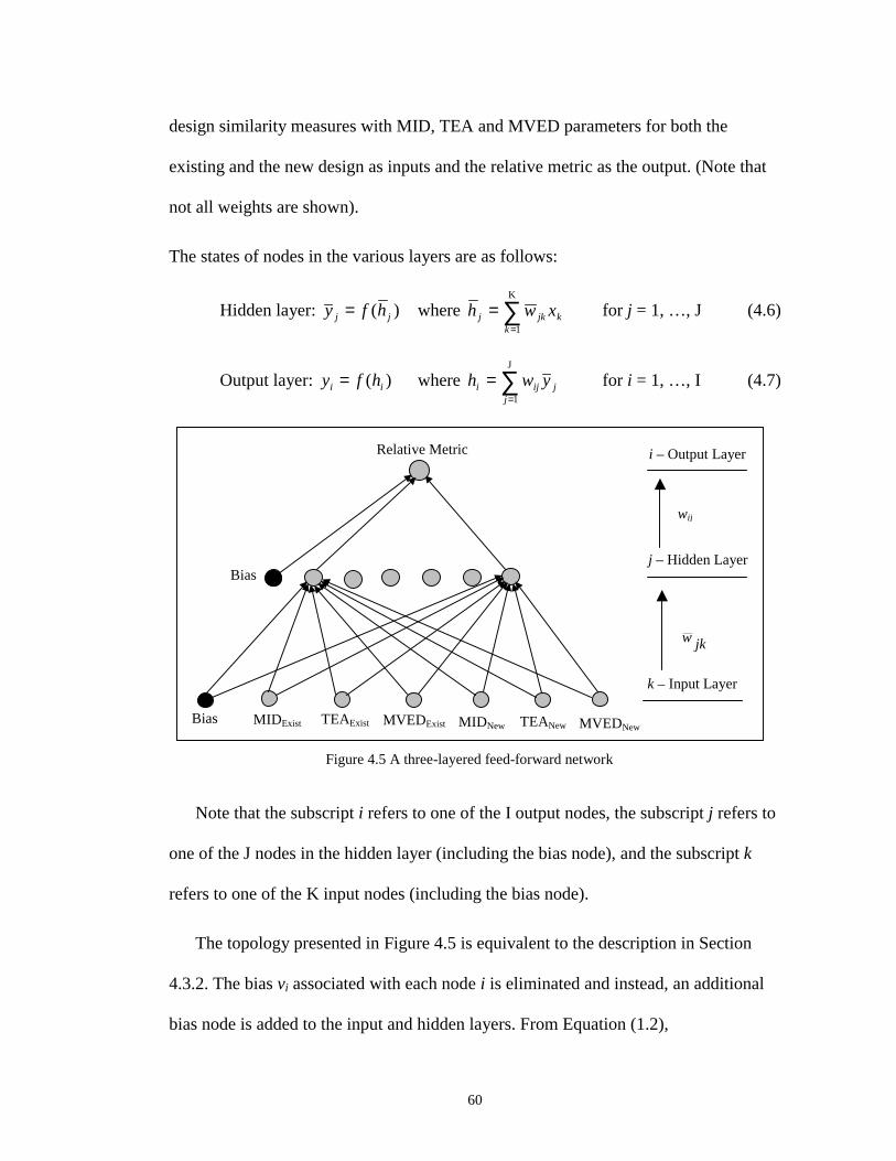
60
design similarity measures with MID, TEA and MVED parameters for both the
existing and the new design as inputs and the relative metric as the output. (Note that
not all weights are shown).
The states of nodes in the various layers are as follows:
Hidden layer: )( jj hfy = where ∑=
=K
1kkjkj xwh for j = 1, …, J (4.6)
Output layer: )( ii hfy = where ∑=
=J
1jjiji ywh for i = 1, …, I (4.7)
Note that the subscript i refers to one of the I output nodes, the subscript j refers to
one of the J nodes in the hidden layer (including the bias node), and the subscript k
refers to one of the K input nodes (including the bias node).
The topology presented in Figure 4.5 is equivalent to the description in Section
4.3.2. The bias vi associated with each node i is eliminated and instead, an additional
bias node is added to the input and hidden layers. From Equation (1.2),
i – Output Layer
j – Hidden Layer
k – Input Layer
wij
jkw
Relative Metric
Bias
Bias MID Exist TEAExist MVEDExist MID New TEANew MVEDNew
Figure 4.5 A three-layered feed-forward network

61
=
−=
−= ∑∑∑
+
=+
==
1J
1)1(
J
1
J
1 jjijiji
jjijii
jjijii swfwswfvswfs (4.8)
where wi(j+1) is the weight associated with the connection between the bias node j+1
(that feeds into node i) and node i. The bias nodes always have a value of 1. In other
words, 100 == yσ . The bias nodes act in a manner equivalent to the intercept term in
regression models. In the example shown in Figure 4.5, there are seven nodes (which
includes the bias node) in the input and hidden layers. The output layer has only one
node.
4.3.6 The Back-Propagation Algorithm
Learning is accomplished through an adaptive procedure, known as a learning rule or
algorithm. Learning algorithms indicate how weights should be incrementally adapted
to improve a predefined performance measure. Learning can be viewed as a search in
a multidimensional weight space for a solution, which gradually optimizes a
predefined objective function [Has95]. Back-propagation is the most extensively used
training method. The back-propagation algorithm is an iterative gradient method based
algorithm developed to introduce synaptic corrections (weight adjustments) by
minimizing the sum of squared error (objective function).
Back-Propagation in a Three-layered Feed-forward Network
The aim is to choose weights such that the output deviation function is minimized. The
output deviation function (sum of squared error) is given as follows:
D = [ ]∑=
−I
1
2
2
1
iii yd (4.9)

62
where i represents an output node, yi = Actual network output; di = Desired output.
Adopting the method of steepest descent, we can determine corrections to weights
as follows [Mul90] (considering connections for the output nodes):
ijijij wtwtw δ+=+ )()1( (4.10)
[ ]ij
iiii
ijij w
hhfyd
w
Dw
∂∂′−=
∂∂−= )(εεδ (4.11)
where ε = learning rate.
For the sigmoidal transfer function [given )( ii hfy = ],
)1()( iii yyhf −=′ (4.12)
jij
i yw
h=
∂∂
(4.13)
Substituting (4.12) and (4.13) in (4.11), we get,
[ ] jijiiiiij yyyyydw ∆=−−= εεδ )1( (4.14)
where [ ] )1( iiiii yyyd −−=∆
For weights associated with synaptic connections between the input and hidden layer,
jkjkjk wtwtw δ+=+ )()1( (4.15)
[ ]∑= ∂
∂∂∂′−=
∂∂−=
I
1
)(i jk
j
j
iiii
jkjk w
y
y
hhfyd
w
Dw εεδ (4.16)
[ ]∑= ∂
∂′′−=
∂∂−=
I
1
)()(i jk
jjijiii
jkjk w
hhfwhfyd
w
Dw εεδ (4.17)
For a sigmoid transfer function,
)1()( jjj yyhf −=′ (4.18)
63
kjk
j xw
h=
∂∂
(4.19)
Substituting (4.18) and (4.19) in (4.17), we get:
∑=
−−−=I
1
)1()1(][i
kjjijiiiijk xyywyyydw εδ (4.20)
[ ]∑=
−−−=I
1
)1()1(i
ijiiiikjjjk wyyydxyyw εδ (4.21)
jkjk xw ∆= εδ where ∑=
∆−=∆I
1
)1(i
ijijjj wyy (4.22)
Convergence can be accelerated by adding a momentum term as follows [Lip87]:
))1()(()()1( −−++=+ twtwwtwtw ijijijijij ηδ (4.23)
))1()(()()1( −−++=+ twtwwtwtw jkjkjkjkjk ηδ (4.24)
where η = momentum factor and 0 < η < 1.
In the region of weight space for which the error surface has relatively low
curvature, it can be shown [Bis95] that the momentum term aids in increasing the
learning rate ε to an effective learning rate of ε /(1-η).
This recursive method of back-propagation can be further extended for networks
with more than one hidden layer. The values for the parameter constants such as ε and
η can be altered to either improve performance or to reduce computational effort. This
is further discussed in Section 4.3.9. There is no general criterion to determine these
constants. The optimal values depend on the problem at hand.

64
Back-Propagation in a Four-layered Feed-forward Network
Here, the subscript j refers to one of the J nodes in the second hidden layer, subscript k
refers to one of the K nodes in the first hidden layer, and the subscript l refers to one
of the L input nodes.
1st Hidden layer: )ˆ(ˆ kk hfy = where ∑=
=L
1
ˆˆl
lklk xwh for k = 1, …, K (4.25)
2nd Hidden layer: )( jj hfy = where ∑=
=K
1
ˆk
kjkj ywh for j = 1, …, J (4.26)
Output layer: )( ii hfy = where ∑=
=J
1jjiji ywh for i = 1, …, I (4.27)
For weights associated with synaptic connections between the input and first
hidden layer,
klklkl wtwtw ˆ)(ˆ)1(ˆ δ+=+ (4.28)
lkkl xw ∆= ˆˆ εδ where ∑=
∆−=∆J
1
)ˆ1(ˆˆj
jkjkkk wyy (4.29)
The Algorithm [Lip87]
1. Initialize all weights to random values. Weight initialization is discussed in
Section 4.3.8.
2. Prepare a data set of input vectors x0, x1, …… xm, with their associated output
vectors d0, d1, …… dm. In our case, we have 729 sets of input/output pairs. Of
this, we reserve 25% (183) for testing (validating) and use the other 546 for
training.

65
3. Present the first input vector for training. Evaluate actual output. Starting at the
output node, work back to the hidden layers and the input layer to adjust the
weights, as described in Section 4.3.6. Then present second input vector, adjust
weights, and repeat for all 546 examples in the training set.
4. At the end of this training cycle, test the network with the testing data set (183 sets
of input/output pairs). Evaluate Mean Absolute Deviation (Other measures can
also be used). If MAD ceases to improve (See Section 4.3.10), stop training and
store weights; else repeat steps 3 and 4 for another training cycle.
Mean Absolute Deviation (MAD) = N
YYN
nnn∑
=
−1
ˆ
(4.30)
where N = Testing sample size (N = 183)
nY = Predicted (actual) output of for sample n
Yn = Desired output of sample n
Figure 4.6 shows a schematic representation of the Back-Propagation Algorithm.
Note that the algorithm described above represents a sequential or incremental
learning approach. An alternative to this technique is the batch mode where weights
are adjusted at the end of each training cycle as against weight correction after each
presentation of an input vector (as seen in the sequential approach). An advantage of
the sequential approach is its relative potential to escape from local minima.
4.3.7 Pre-processing
Neural networks in principle can map raw input values directly into require final
output values. However, in most situations neural networks do not yield satisfactory

66
results without having the input data pre-processed. In many practical applications, the
choice of pre-processing appears to be one of the most significant factors in
determining the performance of the neural network model [Bis95]. It is often
necessary to transform the input data into some new representation before presenting
them to the network.
Each input vector has to be pre-processed before it is passed on to the network.
Sometimes, post-processing of the output values may also be essential. The output
values must be post-processed using a post-processing transformation. In the training
Present Input Vector
Evaluate Output
Adjust Weights
Training
Present Input Vector
Evaluate Output
Absolute Deviation
Testing
Mean Absolute Deviation
Initialize Weights
Prepare Data Set
Figure 4.6 A Schematic representing the Back-Propagation Algorithm

67
phase, the target values must be inverse-transformed to obtain the output values for
training.
Standardization
Standardization is one of the most common techniques in pre-processing input data. It
is essentially a linear scaling of the input variables so that different variables having
values which differ by orders of magnitude can be presented in a manner where the
relative importance of the different input variables in determining the output values is
maintained. For example, in our implementation, the MID, TEA, and the MVED
parameters for both the existing and the new part fall within a range of 40-150, while
the TEA parameter falls within a range of 900-9700. The aim is to transform every
input variable so that every variable in the input vector is of the same order of
magnitude.
Suppose ix is the sample mean of an input variable kx , 2kσ is the sample variance
with respect to the training set of input data.
∑=
=M
m
mkk x
Mx
1
1(4.31)
∑=
−−
=M
mk
mkk xx
M 1
22 )(1
1σ (4.32)
where mkx (m = 1,…,M) is the value of variable kx in the mth input vector of the
training set, and M is the total number of input vectors in the training set.
Each instance of the input variable is transformed as follows:

68
k
kkkm
k
xxx
σ−
=ˆ (4.33)
The re-scaled variable kx , associated with kx in the training set, has a zero mean
and unit standard deviation. Note that each variable is transformed independently. This
ensures that all of the input and output variables are of the order unity, and hence, the
weights would also be restricted to order unity. For the first training iteration, weights
can be randomly initialized restricting them to order unity. In the absence of pre-
processing (and, in some cases, post-processing), weights may have differing orders of
magnitude.
4.3.8 Weight Initialization
Most of the initialization techniques aim at setting weights to randomly chosen small
values. This is required in order to avoid symmetries in the network. The sigmoid
function outputs a value very close to zero or one (in other words, the function is
saturated) if it receives an input that lies outside [-3,3]. Therefore, the initial weights
should be small so that the sigmoid transfer functions are not driven into their
saturation regions. However, if weights are too small, the sigmoidal functions will be
approximately linear. As a result, nonlinearity in the network will be lost and training
will be slower. It is desirable to maintain the summed inputs to sigmoidal functions
within order unity.
Given that the inputs are standardized (rescaled so as to have a zero mean and unit
standard deviation), initial weights can be generated from a Gaussian distribution with
a zero mean and a variance σ2 α 1/d, where d is the number of nodes in the layer

69
where the connections originate [Bis95]. Suppose there are seven input neurons
feeding into the first hidden layer and thirteen nodes in the hidden layer feeding into
the output layer. Weights associated with arcs that connect nodes in the input layer to
nodes in the hidden layer are generated with a standard deviation σ α 1/√7, while
weights associated with arcs that connect nodes in the hidden layer to nodes in the
output layer are generated with a standard deviation σ α 1/√13. In our
implementation, σ = 1/√d.
4.3.9 Adaptive Learning
Setting a value for the learning rate is essentially a trade-off between speed of
convergence and the ability to closely approximate the gradient path. When ε is small,
convergence will be slow due to a large number of update steps needed to reach a
local minima. With a large ε, convergence is fast initially, but will induce oscillations
and the error function will not reach a minimum [Lin97]. One possible strategy
[Has95] is to use a large step size when the iteration is far from a minimum and a
decreasing step size when the iteration approaches a minimum. However, this induces
oscillations around the region where there is a decrement in the learning rate.
Therefore, in practice, a constant value for the learning rate is used as this generally
leads to better results even though the guarantee of convergence is lost [Bis95].
Another heuristic [Has95] to accelerate learning is to use learning rates, specific
for each node, which are proportional to the number of nodes that feed in. If there are
seven nodes in the input layer and thirteen nodes in the hidden layer, the learning rate

70
for each node in the hidden layer is inversely proportional to seven, while that for each
node in the output layer is inversely proportional to thirteen.
4.3.10 Cross-Validation
When the performance of a network is determined by evaluating the error function
with respect to an independent testing (validating) data, it is observed that the
validation error decreases monotonically to a minimum but then starts to increase. In
general, multiple local minima may also exist in the validation error curves. This is
attributed to excessive training, when training with noisy data, leading to over-fitting.
Therefore, training is continued as long as performance on the validation set keeps
improving. The set of weights that yields the least MAD is retained. This method of
partial training may lead to a better generalization.
4.3.11 Implementation Results
This section presents some of the preliminary results and observations for the
proposed model for design similarity prediction. As mentioned earlier, there is no
methodology to select the number of hidden layers, number of nodes in each hidden
layer, connectivity, and a learning algorithm. This necessitates constructing networks
with different values for the model parameters to find the optimal configuration.
The set of 27 designs and their fixtures, that were used to investigate the single
attribute measures, were used for network training and testing. The relative usefulness
metrics of each design on itself and all other designs were evaluated. This yielded 729
(272) pairs of designs, each with a relative usefulness metric. Note that, a fixture

71
yields a relative usefulness metric of 1 with its own design. In other words, the relative
metric for a design with itself is equal to 1.
Feed-forward networks with sigmoid activation functions for hidden and output
layers are considered. Learning is by the Least Mean Square based Back Propagation
Algorithm described in Section 4.3.6. The learning rate for a network is represented by
ε′. However, the learning rate for each node is determined by the heuristic [Has95]
described in Section 4.3.9. For example, for a three-layered network with number of
hidden nodes = 13, ε′ = 0.07, learning rate for the hidden layer = ε′ /7 = 0.07/7 = 0.01,
while the learning rate for the output layer = ε′ /13 = 0.07/13 = 0.0054.
When ε′ is set at a relatively small value, the algorithm gets caught in local minima
and does not approach the global minimum. Oscillations are observed as the learning
rate is increased (See Figure 4.7). An appropriate range of learning rate values is
Figure 4.7 Oscillations are observed when ε′ = 0.5 for a three-layered network withseven nodes in the hidden layer.

72
determined and the network is tested for different values of learning rate in this range.
In our implementation, the momentum factor is maintained at η = 0.9 for all
experiments. Experiments are conducted for networks with one and two hidden layers,
while the number of hidden nodes is set at either seven or thirteen (including the bias
node). Neglecting the bias nodes in the hidden and input layers, a network with seven
nodes in the hidden layer has equal number of hidden nodes and input nodes, while a
network with thirteen nodes in the hidden layer has two hidden nodes for every input
node. The results are tabulated in Table 4.1. A configuration is specified by the
number of hidden layers n1, number of hidden nodes n2, and a learning rate ε′. f(n1, n2,
ε′) is the minimum MAD observed in 5000 training cycles.
A network with two layers and seven nodes in the hidden layer is identified as the
optimal network model and the associated minimum MAD is 0.206576. However,
these experiments are not exhaustive. By further varying learning rates and
momentum parameters, we might arrive at a better network structure. Note that there
Table 4.1 Network performance (MAD) versus network structure
ε′ f(1,7, ε′) f(1,13, ε′) f(2,7, ε′) f(2,13, ε′)0.01 0.217768
0.04 0.219189 0.211462 0.215588 0.210713
0.05 0.214961 0.213404 0.210757
0.07 0.209749 0.21449 0.209364 0.216243
0.09 0.210894 0.217342 0.206576 0.207592
0.1 0.216591 0.218244 0.210914 0.21443
0.2 0.208051 0.21481
0.3 0.207501 0.215314 0.207629
0.5 0.216103

73
is little or no improvement with increase in the number of hidden layers or the number
of nodes within each hidden layer.
4.4 Comparison of Design Similarity Measures
A comparison of the neural network model performance against the performance of
other measures based on MID, TEA and MVED is presented below. An ideal fixture-
based design similarity measure is one where a higher value for the similarity measure
implies a higher fixture usefulness. This is equivalent to saying that the design
similarity measure and the relative usefulness metric are perfectly correlated. Table
4.2 shows the correlation coefficient between the design similarity measure against the
desired relative metric for measures based on MID, TEA, MVED and the Neural net.
The neural network-based design similarity measure performs better than the other
models and exhibits a high correlation.
For ten new designs, we compared the best existing fixture identified by different
similarity measures to the best generatively designed fixture (See Table 4.3). An
observation of the relative metric (ratio of usefulness for the existing fixture of the
most similar part to the usefulness of the generatively designed fixture) of these
identified fixtures indicates that the neural network model, on an average, identifies a
fixture with a higher usefulness metric. In other words, the average relative metric for
Table 4.2 Correlation coefficients for various design similarity measures
MID TEA MVED Neural NetworkCorrelationCoefficient
0.3593 0.3432 0.1558 0.6001

74
Usefulness Metric of Most Similar Part Relative Metric of Most Similar PartNewPart
Number
MID(Metric)
TEA(Metric)
MVED NeuralNet
GenerativeFixtureMetric
MID(RelativeMetric)
TEA(RelativeMetric)
MVED(RelativeMetric)
Neural Net(RelativeMetric)
1 7.37 0 11.399 14.629 69.292 0.1064 0 0.1645 0.2111
2 20.975 0 21.617 22.344 69.717 0.3009 0 0.3101 0.3205
3 0 0 0 7.832 13.229 0 0 0 0.592
4 0 0 0 16.148 33.773 0 0 0 0.4781
5 0 15.595 15.584 28.454 33.549 0 0.4648 0.4645 0.8481
6 0 0 0 0.695 23.366 0 0 0 0.0297
7 3.768 0 0 0 36.504 0.1032 0 0 0
8 13.977 13.977 13.977 16.726 16.726 0.8356 0.8356 0.8356 1
9 15.426 0 21.127 21.127 28.253 0.546 0 0.7478 0.7478
10 0 0 0 7.36 8.334 0 0 0 0.8831
Average 0.1892 0.13 0.2523 0.5111
Table 4.3 Performance of the different design similarity measures in identifying the best existing fixture

75
the best existing fixture identified by the different measures is highest for fixtures
identified by the neural network model. Also, the design similarity measure based on
the neural network model identifies a better fixture in nine out of the ten cases. Note
that the computational effort required to train the network, in the preparatory stage, for
a neural network-based measure is considerably higher compared to the other
measures. However, in the production stage, the effort required to sort the existing
fixtures and the subsequent effort to find the usefulness of an existing fixture is
comparable for all the measures. See Section 4.6 for an evaluation of the order of
complexity associated with finding the usefulness of an existing fixture.
4.5 A Complete Example
This section presents a complete example illustrating the application of the variant
fixture planning methodology. This example also describes the variant fixture planner
from an end-user perspective and highlights the impact of the work presented in this
thesis.
The variant fixture planner was developed in Visual Basic reusing some of the
routines from FixtureNet. All operations related to the variant fixture planner and
design similarity measures are contained in the menu called DSMs. The user can input
a new part (generated using the drawing tool provided by FixtureNet) using the Input
New Part option. Figure 4.8 shows the 2D projection of a new part. Any of the
different design similarity measures (represented by MID, TEA, MVED, and NNet in
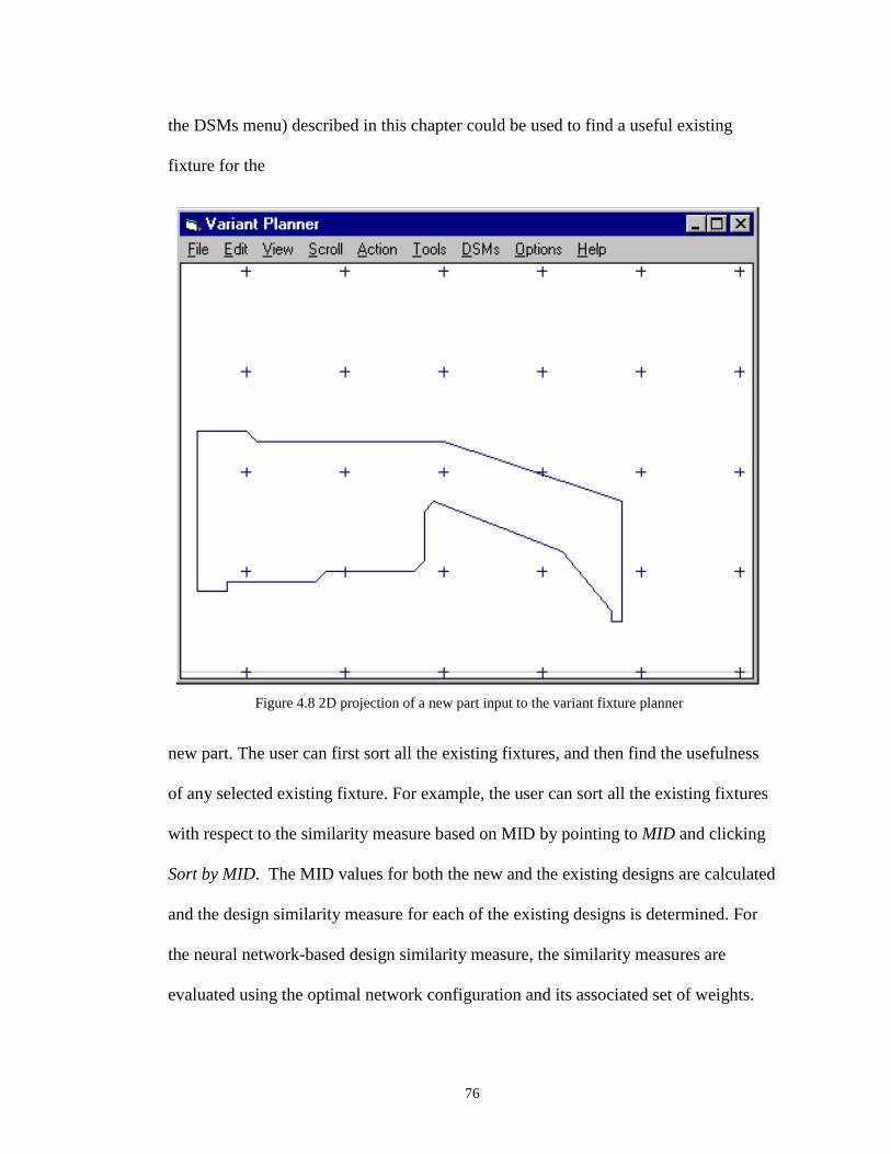
76
the DSMs menu) described in this chapter could be used to find a useful existing
fixture for the
new part. The user can first sort all the existing fixtures, and then find the usefulness
of any selected existing fixture. For example, the user can sort all the existing fixtures
with respect to the similarity measure based on MID by pointing to MID and clicking
Sort by MID. The MID values for both the new and the existing designs are calculated
and the design similarity measure for each of the existing designs is determined. For
the neural network-based design similarity measure, the similarity measures are
evaluated using the optimal network configuration and its associated set of weights.
Figure 4.8 2D projection of a new part input to the variant fixture planner

77
The existing designs are sorted in descending order based on the design similarity
measure. The fixture usefulness of a selected existing fixture (steps 2 and 3 in variant
fixture planning algorithm described in Section 4.1.2) can be evaluated by clicking
Find Usefulness. The usefulness of all the existing fixtures with respect to a design
similarity measure also can be evaluated. For example, the usefulness of all the
existing fixtures with respect to the design similarity measure based on MID can be
evaluated by pointing to MID and clicking Find All Metrics.
The number of layers in the network can be specified by pointing to NNet, clicking
Number of Layers, and then pointing to either Three_Layer or Four_Layer. The
number of hidden nodes in each hidden layer can be specified by pointing to NNet and
clicking Number of Hidden Nodes. The network can be initialized either with random
weights or from a file (point to NNet and click Random Weights or Weights from File).
If one needs to continue training a network after having terminated on reaching a
predefined number of cycles, the stored weights could be used to initialize the
network. A neural network, subsequent to initialization, can be trained by pointing to
Train Network. Weights corresponding to the least MAD are output to a file. These
weights are used to evaluate the design similarity measure for any existing design with
respect to a new design.
The optimal neural network with two hidden layers with seven nodes in each is
used in this example to determine the design similarity measures. Figure 4.9 lists the
existing designs sorted by their design similarity measures with the new part. From
Figure 4.9, it is apparent that the existing design with Part ID 25 holds the highest
promise. While the next 15 designs are relatively less promising, the other designs are
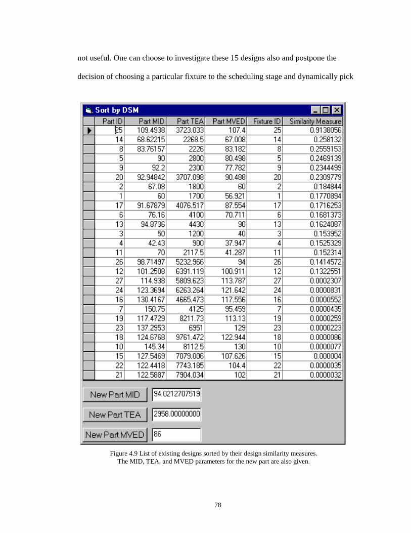
78
not useful. One can choose to investigate these 15 designs also and postpone the
decision of choosing a particular fixture to the scheduling stage and dynamically pick
Figure 4.9 List of existing designs sorted by their design similarity measures.The MID, TEA, and MVED parameters for the new part are also given.

79
a fixture based on the current state of the shop. This issue is revisited in Chapter 5.
A total of five configurations were identified for the new part with the locator
triplet from the existing fixture. For each configuration, new clamp positions are
enumerated. A total of ten new fixtures are designed, with the best fixture yielding a
Figure 4.10 The new part in the locator triplet from the best existing fixture identifiedusing the design similarity measure

80
usefulness metric of 28.454, as shown in Figure 4.10. Figure 4.11 shows the new part
with its best generatively designed fixture. The associated usefulness metric is 35.549.
Hence, the relative usefulness metric for the fixture associated with the most
promising existing design (Part ID 25) is given by 28.454/35.549 = 0.8.
Figure 4.11 The new part with its best generatively designed fixture

81
4.6 Order of Complexity
The variant approach requires less computational effort than the generative approach.
In Section 3.3.8, it was shown that the generative procedure requires O(n5 d5) effort,
where n is the number of edges for a given polygonal part and d is the length of its
maximum diameter (in units of lattice spacing).
In the variant approach, the computational effort required to determine the
usefulness of an existing fixture for a new part is as follows:
For an existing locator triplet, identifying feasible configurations: O(n3)
For each part configuration, enumerating feasible clamp positions: O(nd)
For each fixture, checking for unwanted collisions: O(n)
Total computational effort: O(n5 d)
Therefore, the difference in computational effort is more significant when the part size
is large compared to the lattice spacing on the base plate. If each existing fixture’s
usefulness has to be determined, and if the database is large, the benefit in
computational effort is reduced. Hence, the use of a design similarity measure helps to
further reduce the computational effort by identifying promising fixtures. For each
promising fixture, a precise usefulness metric is evaluated.
4.7 Summary
This chapter presented a variant fixture planning approach that uses a fixture-based
design similarity measure to find promising fixtures quickly. The variant fixture
planning approach was developed reusing some of the routines from FixtureNet

82
described in Chapter 3. Hence, all the limitations that were listed for the generative
planner are also applicable for the variant approach. This approach avoids checking
the feasibility of each existing fixture. For each promising fixture, the approach
calculates a more precise usefulness metric that describes how well the fixture can
hold the new design.
Design attributes that reflect fixture usefulness were identified. Design similarity
measures based on any of these design attributes were been discussed. The use of
neural networks to represent the mapping between design attributes and fixture
usefulness has been explored. Compared to other measures based on design attributes
that reflect fixture usefulness, the neural network-based design similarity measure
exhibits better consistency and, on average, identifies an existing fixture with a higher
usefulness metric.

83
Chapter 5
Conclusions and Future Work
The variant fixture planner described in this thesis forms part of a hybrid variant-
generative process planning system. The variant fixture planning approach uses a
fixture-based design similarity measure to find efficiently identify promising fixtures.
This approach avoids checking the feasibility of each existing fixture. For each
promising fixture, the approach calculates a more precise usefulness metric that
describes how well the fixture can hold the new design.
A generative fixture synthesis algorithm, and FixtureNet, an online interactive
computer aided fixture design system based on this algorithm (developed by Richard
Wagner, Ken Goldberg, Xiaofei Huang and Randy Brost [Bro96]) was described. This
algorithm enumerates all admissible fixtures for an arbitrary polygonal part projection.
A variant fixture planning methodology was described that retrieves, for a new product
design, a useful fixture from a given set of existing designs and their fixtures. Several
design attributes that reflect fixture usefulness were identified. A generic design
similarity measure based on a single design attribute was described. The use of neural
networks to represent the mapping between design attributes and fixture usefulness

84
was explored. Compared to other measures based on design attributes that reflect
fixture usefulness, the neural network-based design similarity measure exhibited better
consistency and, on average, identified an existing fixture with a higher usefulness
metric. A variant fixture planner was developed as an extension to FixtureNet to
implement the variant fixture planning methodology developed in this thesis. A
complete example also was presented to illustrate the application of the variant fixture
planning approach, and to provide an end-user perspective. Section 5.1 discusses the
anticipated impact and contributions of the work described in this thesis. Section 5.2
lists research issues not addressed in this thesis, challenges to the variant fixture
planning approach described in this thesis, and avenues for future work.
5.1 Anticipated Impact
A modular fixture system is flexible because one can construct a large number of
fixture configurations from different combinations of high precision standard fixture
elements. However, redesigning and reconfiguring modular fixtures cost money and
time. By using modular fixture components to set up a dedicated fixture of high
precision, one can achieve reuse of existing fixtures and fixturing solutions, with
minor modifications. This results in a reduction in the amount of time and resources
spent on constructing new fixtures.
FixtureNet could be extended to generate fixtures that are fabricated with a plain
tooling plate. The variant fixture planning algorithm described can therefore be
extended for reuse of dedicated fixtures fabricated with a plain tooling plate.

85
The computational effort required in evaluating the usefulness of an existing
fixture for a new design is considerably less compared to designing a new fixture
generatively. This difference is more significant when the part size is large compared
to the lattice spacing on the base plate.
Any new design can be grouped together, to reduce changeover times, with an
existing design whose fixture is useful for the new design. It might be economical to
dynamically assign a new design to an existing fixture with a relatively inferior fixture
usefulness (compared to other existing fixtures that might be useful the new design), if
the two parts can be grouped together in production.
5.2 Avenues for Future Work and Challenges
The variant approach was developed to form part of a hybrid variant-generative
process planning methodology. This requires integration of the variant fixture
approach with a generative process planning approach that creates a preliminary
process plan.
Once the variant planner presents a list of promising existing fixtures, one can
dynamically choose to pursue those fixtures based on the current state of the shop
floor. To achieve this, the fixture planner has to be integrated with a shop floor
scheduling engine.
The variant approach described in Chapter 4 assumes an infinite base plate. In
other words, when an existing fixture is found to be useful for a new design, it is
assumed that the new part when held with the fixture designed with the variant

86
approach lies within the bounds of the base plate. An explicit step can be incorporated
into the algorithm to compare the bounds of the new part configuration against the
bounds of the base plate.
The approach can be extended to other metrics that a shop might consider
important. The network can be retrained to reflect fixture usefulness with respect to
the new quality metric. However, a workpiece might typically be subjected to different
machining operations in a single setup, and different machining operations might
necessitate the use of different quality metrics. Hence, a design similarity measure that
incorporates different metrics would be desirable.
The current approach does not include verification of the retrieved fixture to check
if the fixture is indeed feasible in all respects. A fixture might provide deterministic
location and total restraint but might pose problems when loading the workpiece
against the locators. In the case of designs with thin wall sections, the retrieved fixture
might not provide sufficient support.
For the variant planner to be effective, maintaining the integrity of the database of
existing designs and fixtures is paramount. The database has to be up-to-date and
should record any fixture design modification or reconfiguration over time, and if
required, the neural network must be retrained.

87
BIBLIOGRAPHY
[Asa85] Asada, H. and By, A. B., “Kinematic Analysis of Workpart Fixturing for
Flexible Assembly with Automatically Reconfigurable Fixtures,” IEEE J.
of Robotics and Automation, Vol. RA-1, No. 2, p. 86-94, 1985.
[Bal98] Balasubramanian, S., Elinson, A., Herrmann, J. W., Nau, D. S., “Fixture-
based usefulness measures for hybrid process planning,” 1998 ASME
Design Engineering Technical Conferences, Atlanta, Georgia, September
13-16, 1998.
[Boe88] Boerma, J. R., and Kals, H. J. J., “FIXES, a System for Automatic
Selection of Set-ups and Design of Fixtures,” Annals of the CIRP, Vol. 37,
No. 1, p. 443-446, 1988.
[Bro91] Brost, R. C., “Analysis and planning of planar manipulation tasks,”
Technical Report CMU-CS-91-149, Carnegie Mellon University,
Pittsburgh, PA, 1991.
[Bro96] Brost, R. C. and Goldberg, K. Y., “A Complete Algorithm for Designing
Planar Fixtures using Modular Components,” IEEE Transactions on
Robotics and Automation, Vol. 12, No. 1, February 1996.
[Cha92] Chang, C.-H., “Computer-Assisted Fixture Planning for Machining
Processes,” Manufacturing Review, Vol. 5, No. 1, p. 15-28, 1992.
[Cha98] Chang , T. C., Wysk, R. A., and Wang, Hsu-Pin, “Computer-Aided
Manufacturing,” 2nd Edition, Prentice Hall, 1998.

88
[Cho94] Chou, Y.-C., Srinivas, R. A. and Saraf, S., “Automatic Design of
Machining Fixtures: Conceptual Design,” Intl. J. of Advanced
Manufacturing Technology, Vol. 9, p. 3-12, 1994.
[Chr91] Chryssolouris, G., Lee, M. and Domroese, M., “The Use of Neural
Networks in Determining Operational Policies for Manufacturing
Systems,” J. of Manufacturing Systems, Vol. 10, No. 2, p. 166-175, 1991.
[Dar90] Darvishi, A. R. and Gill, K. F., “Expert System Rules for Fixture Design,”
Intl. J. of Production Research, Vol. 28, No. 10, p. 1901-1920, 1990.
[Eli97] A. Elinson, J.W. Herrmann, I. Minis, D. S. Nau, and G. Singh, “Toward
Hybrid Variant/Generative Process Planning,” Design for Manufacturing
Symposium, ASME Design Engineering Technical Conference,
Sacramento, California, September 14- 17, 1997.
[Fer88] Ferreira, P. M. and Liu, C. R., “Generation of Workpiece Orientation for
Machining using a Rule-based System,” Robotics and Computer Integrated
Manufacturing, Vol. 4, No. 3/4, p. 545-555, 1988.
[Fuh93] Fuh, J. Y. H., Chang, C.-H., Melkanoff, M. A., “An Integrated Fixture
Planning and Analysis System for Machining Processes,” Robotics and
Computer-Integrated Manufacturing, Vol. 10, No. 5, p. 339-353, 1993.
[Gan86] Gandhi, M. V., Thompson, B. S., “Automated Design of Modular Fixtures
for Flexible Manufacturing Systems,” J. of Manufacturing Systems, Vol. 5,
No. 4, p. 243-252, 1986.

89
[Gup94] S. K. Gupta, D. S. Nau, W. C. Regli, and G. Zhang, “A methodology for
systematic generation and evaluation of alternative operation plans,” In
Jami Shah, Martti Mantyla, and Dana Nau, editors, Advances in Feature
Based Manufacturing, p. 161--184. Elsevier/North Holland, 1994.
[Har94] Hargrove, S. K. and Kusiak, A., “Computer-aided Fixture Design: a
Review,” Intl. J. of Production Research, 1994, Vol. 32, No. 4, p. 733-753.
[Has95] Hassoun, Mohamad H., “Fundamentals of Artificial Neural Networks,”
The MIT Press, Cambridge, Massachussetts, 1995.
[Her97] Herrmann, Jeffrey W., and Gurdip Singh, “Design similarity measures for
process planning and design evaluation,” Technical Report 97-74, Institute
for Systems Research, University of Maryland, College Park, 1997.
[Hof84] Hoffman, Edward G., “Fundamentals of Tool Design,” Prentice-Hall, Inc.,
Englewood Cliffs, New Jersey, 1984.
[Hof87] Hoffman, Edward G., “Modular Fixturing,” Manufacturing Technology
Press, Inc., Lake Geneva, Wisconsin, 1987.
[Hua99] Huang, C. –L., Huang, Y. –H., Chang, T. –Y., Chang, S. –H., Chung, C. –
H., Huang, D. –T. and Li, R. –K., “The Construction of Production
Performance Prediction System for Semiconductor Manufacturing with
Artificial Neural Networks,” Intl. J. of Production Research, Vol. 37, No.
6, p. 1387-1402, 1999.

90
[Leu94] Leung, H. C., Hines, E. L., Raja, V. H., “The Application of Artificial
Neural Networks in Computer Aided Process Planning,” Proceedings of
Intelligent Engineering Systems through Artificial Neural Networks,
November 13-16, St. Louis, MO, 1994, p. 1091-1096.
[Lin97] Lin, Z.-C. and Huang, J.-C., “The Applications of Neural Networks in
Fixture Planning by Pattern Classification,” J. of Intelligent
Manufacturing, Vol. 8, p. 307-322, 1997.
[Lip87] Lippmann, Richard P., “An Introduction to Computing with Neural Nets,”
IEEE ASSP Magazine, p. 4-22, April, 1987.
[Mar94] Marefat, M., and Britanik, J., “Case-based Process Planning with
Hierarchical Plan Merging,” 1994 IEEE Intl. Conference on Systems, Man,
and Cybernetics, Humans, Information and Technology, Vol. 1, p. 165-
170, 1994.
[Mul90] Muller, B. and Reinhardt, J., “Physics of Neural Networks, Neural
Networks: An Introduction,” Springer-Verlag, 1990.
[Nee91] Nee, A. Y. C., “A Framework for an Object/Rule-based Automated Fixture
Design System,” Annals of the CIRP, Vol. 40, No. 1, 1991.
[Nee92] Nee, A. Y. C., Senthil Kumar, A., Prombanpong, S., Puah, K. Y., “A
Feature-based Classification Scheme for Fixtures,” Annals of the CIRP,
Vol. 41, No. 1, p. 189-192, 1992.

91
[Ngu88] Nguyen, V.-D., “Constructing Force-Closure Grasps,” Intl. J. of Robotics
Research, Vol. 7, No. 3, p. 3-16, June 1988.
[Nna89] Nnaji, B. O., Alladin, S., Lyu, P., “A Framework for a Rule-based Expert
system for Face Milling Planer Surfaces on a CAD System using Flexible
Fixtures,” J. of Manufacturing Systems, Vol. 7, No. 3, p. 193-207, 1989.
[Phi94] Philipoom, P. R. and Rees, L. P., Wiegmann, L., “Using Neural Networks
to Determine Internally-Set Due-Date Assignments for Shop Scheduling,”
Decision Sciences, Vol. 25, p. 825-851, 1994.
[Sen92] Senthil Kumar, A., Nee, A. Y. C. and Prombanpong, S., “Expert Fixture-
design System for an Automated Manufacturing Environment,” Computer
Aided Design, Vol. 24, No. 6, p. 316-326, June 1992.
[Sen95] Senthil Kumar A. and Nee A. Y. C., “A Framework for a Variant Fixture
Design System using Case-based Reasoning Technique,” MED
Manufacturing Science and Engineering Proceedings, San Francisco, CA,
November 12-17, 1995, Vol. 2-1, p. 763-775.
[Shi93] Shirinzadeh, B., “Issues in the Design of the Reconfigurable Fixture
Modules for Robotic Assembly,” J. of Manufacturing Systems, Vol. 12,
No. 1, p. 1-14, 1993.
[Sin97] Singh, Gurdip, “A Plan-Based Design Similarity Approach for Hybrid
Process Planning,” Technical Report 97-4, Institute for Systems Research,
University of Maryland, College Park, 1997.

92
[Tra90] Trappey, J. C. and Liu, C. R., “A Literature Survey of Fixture-Design
Automation,” Intl. J. of Advanced Manufacturing Technology, Vol. 5, No.
3, p. 240-255, 1990.
[Yue94] Y., Yue and J. Murray, “Workpiece selection and clamping of complex
2.5D components,” in J. Shah, M. Mäntylä, and D. Nau, Eds., Advances in
Feature Based Manufacturing, Elsevier, Amsterdam, 1994, p. 185–214.
[Wil95] Wilhelm, M., Smith, A. E., Bidanda, B., “Integrating an Expert System and
a Neural Network for Process Planning,” Engineering Design and
Automation, Vol. 1, No. 4, p. 259-269, 1995.
[Zha95] Zhang, H. –C. and Huang, S. H., “Applications of Neural Networks in
Manufacturing: a state-of-the-art survey,” Intl. J. of Production Research,
Vol. 33, No. 3, p. 705-728, 1995.
[Zhu96] Zhuang, Y., Goldberg, K. Y., “On the Existence of Solutions in Modular
Fixturing,” Intl. J. of Production Research, Vol. 15, No. 6, p. 646-656,
1996.
[Zhu97] Zhuang, Y. and Goldberg, K. Y., “Design Rules for Tolerance-Insensitive
and Multi-purpose Fixtures,” Proceedings of the 1997 8th International
Conference on Advanced Robotics, July 7-9, Monterey, CA, 1997, p. 681-
686.