Embed Size (px)
Citation preview

I Raggi Cosmici Parte 2a: Le Energie Elevate

G.Battistoni 2014
Obiettivi della fisica dei Raggi Cosmici: dare una risposta a domande che coinvolgono astrofisica, fisica delle particelle e dei nuclei
1. Quale meccanismo fisico e’ capace di accelerare protoni e nuclei fino a queste energie estreme? (abbiamo dei modelli fino a ~ 1015 eV)
2. Perche’ lo spettro in energia ha questo andamento?
3. Come varia la composizione nucleare dei raggi cosmici alle energie piu’ elevate?
4. Quale e’ l’origine dei cambi di pendenza nello spettro (il “ginocchio”, la “caviglia”)
5. I raggi cosmici sono di orgine galattica o extra? 6. Esistono sorgenti astrofisiche identificabili dei
raggi cosmici? 7. Esiste un’energia limite per i raggi cosmici?

Hadronic cascades
19
//
//
p
iµ
p
K
6 km
12 kmLow energy High energy
Typical energies abovewhich particles interact
EK ⇠ 200GeV
Ep0 ⇠ 1019 eV
Ep± ⇠ 30GeV
em. shower

Electromagnetic showers: Heitler model
Dep
th X
(g/
cm2 )
Number of charged particles
�em
Nmax = E0/Ec
Xmax � �em ln(E0/Ec)
Shower maximum:
E0
E = Ec
E = E0/2nX = n �em
21

Electromagnetic showers: Cascade equations
22
dEdX
=�a� EX0
Energy lossof electron:
Ec = a X0 ⇠ 85MeVCritical energy:
Cascade equations
(Rossi & Greisen, Rev. Mod. Phys. 13 (1940) 240)
+Z •
E
sghmairi
Fg(E)Pg!e(E,E)dE + a∂Fe(E)∂E
dFe(E)dX
=� se
hmairiFe(E)+
Z •
E
se
hmairiFe(E)Pe!e(E,E)dE
Xmax
⇡ X0
ln
✓E
0
Ec
◆N
max
⇡ 0.31pln(E
0
/Ec)�0.33
E0
Ec
X0 ⇠ 36g/cm2Radiation length:
G.Battistoni 2014 6
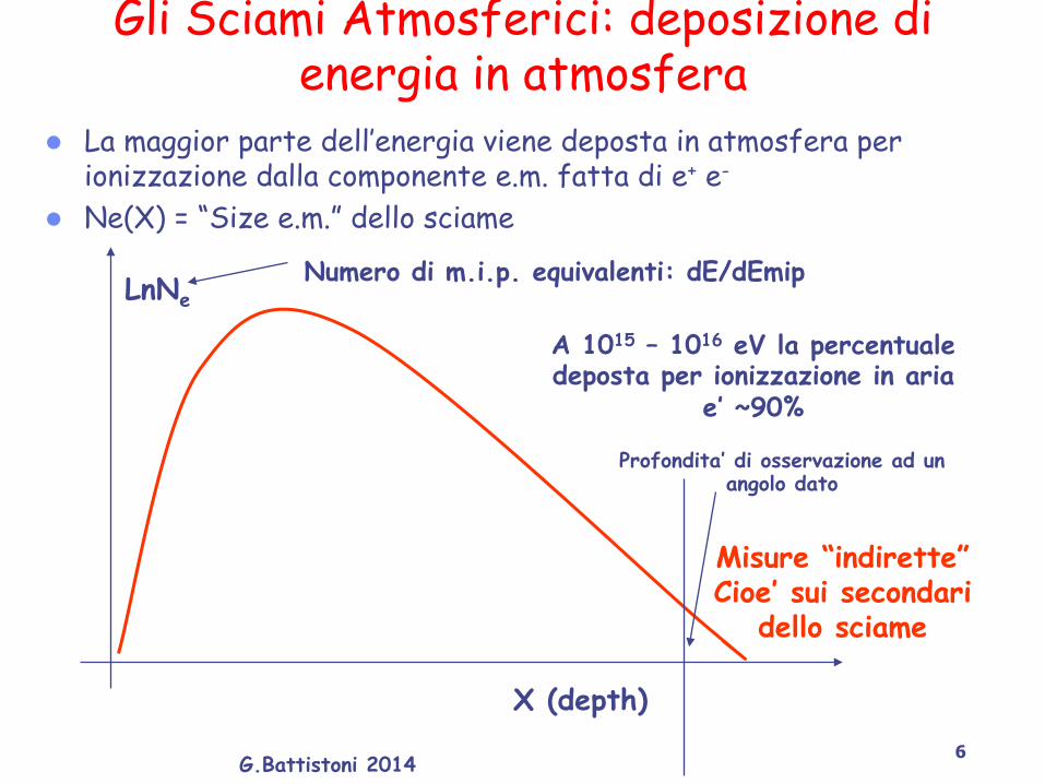
Gli Sciami Atmosferici: deposizione di energia in atmosfera
l La maggior parte dell’energia viene deposta in atmosfera per ionizzazione dalla componente e.m. fatta di e+ e-
l Ne(X) = “Size e.m.” dello sciame
LnNe
X (depth)
Numero di m.i.p. equivalenti: dE/dEmip
A 1015 – 1016 eV la percentuale deposta per ionizzazione in aria
e’ ~90%
Profondita’ di osservazione ad un angolo dato
Misure “indirette” Cioe’ sui secondari
dello sciame

Mean longitudinal shower profile
23
0
2000
4000
6000
8000
10000
x 10
num
ber o
f e- +e
+
e-+e+ cutoff : 1.0 MeV a at E=1014 eV and 0o
Cascade Eqs.
CONEX (hybrid)
CORSIKA
0
2000
4000
6000
8000
x 10 3
200 400 600 800 1000 depth (g/cm2)
num
ber o
f e- +e
+
e-+e+ cutoff : 1.0 MeV a at E=1016 eV and 0o
E = 1014 eV
E = 1016 eV
Calculation with cascade Eqs.
Photons• Pair production• Compton scattering
Electrons• Bremsstrahlung• Moller scattering
Positrons• Bremsstrahlung• Bhabha scattering
(Bergmann et al., Astropart.Phys. 26 (2007) 420)

Energy spectra of secondary particles
24
1000
2000
x 10 4
EdN
/dE
a
a at E=1016 eV and 0o 700 g/cm2
CONEX (MC)Cascade Eqs.CONEX (hybrid)CORSIKA
1000
2000
x 10 3
EdN
/dE
e-
500
1000
1500
x 10 3
10 -3 10 -2 10 -1 1 energy (GeV)
EdN
/dE
e+
(Bergmann et al., Astropart.Phys. 26 (2007) 420)
Photons
Electrons
Positrons
e–
e+
Number of photons divergent
• Typical energy of electronsand positrons Ec ~ 80 MeV
• Electron excess of 20 - 30%
• Pair production symmetric
• Excess of electrons in target

G.Battistoni 2014 9
Quanti muoni arrivano a terra in ogni evento (sciame)?
Toy model dello sciame adronico
(sulla falsariga del toy model dello sciame e.m. di Heitler) Dividiamo l’atmosfera in strati di spessore d = λint ln 2 La lunghezza di interazione e’ molto maggiore della lunghezza di radiazione (per protoni λint ~ 80 g/cm2, per pioni λint ~ 120 g/cm2) pertanto, rispetto alla componente e.m., la componente adronica conserva una frazione maggiore dell’energia dello sciame e ad una profondita’ maggiore

Muon production in hadronic showers
Primary particle proton
π0 decay immediately
π± initiate new cascades
Assumptions: • cascade stops at
• each hadron produces one muon
Epart = Edec
Nµ =�
E0
Edec
⇥�
� =lnnch
lnntot� 0.82 . . .0.95
(Matthews, Astropart.Phys. 22, 2005) 25
E0
/(ntot
)n
E0
/(ntot
)2
E0
/ntot
E0n
tot
= np0
+nch
(nch)2
(nch)n
nch
oooo

Superposition model
26
Proton-induced shower
Nµ =�
E0
Edec
⇥�
Nmax = E0/Ec
Assumption: nucleus of mass A and energy E0 corresponds to A nucleons (protons) of energy En = E0/A
Xmax � �eff ln(E0)
XAmax � �eff ln(E0/A)
NAµ = A
�E0
AEdec
⇥�= A1��Nµ
NAmax = A
�E0
AEc
⇥= Nmax
�� 0.9

Superposition model: correct prediction of mean Xmax
56
42
39
24
iron nucleus
Depth X
Number ofnucleons without interaction
56
4239
2456 protons
iron
npart =�Fe�air
�p�air
Glauber approximation (unitarity)
Superposition and semi-superposition models applicable to inclusive (averaged) observables
(J. Engel et al. PRD D46, 1992)
27
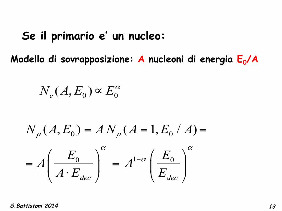
Se il primario e’ un nucleo:
G.Battistoni 2014 13
Modello di sovrapposizione: A nucleoni di energia E0/A
0 0
10 0
( , ) ( 1, / )
dec dec
N A E AN A E A
E EA AA E E
µ µ
α α
α−
= = =
⎛ ⎞ ⎛ ⎞= =⎜ ⎟ ⎜ ⎟
⋅⎝ ⎠ ⎝ ⎠
0 0( , )eN A E Eα∝

G.Battistoni 2014 14
Profilo dello sciame e modello di sovrapposizione � Allo stesso angolo di zenith:
LnNe
Profilo di sciame di protone di energia E
Profilo di sciame da nucleo di massa A ed energia E/A Equivale a A sciami di energia E/A
Ad una depth fissata in atmosfera, a parita’ di energia e angolo di zenit, lo sciame da nucleo
avra’ meno size di uno scimae da protone

G.Battistoni 2014 15
Il profilo longitudinale

G.Battistoni 2014 16
Come varia il profilo longitudinale
Vero in media: grandi fluttuazioni evento per evento! exp(-X/λ)

G.Battistoni 2014 17
Lo sviluppo di uno sciame di un protone primario

G.Battistoni 2014 18
Lo sviluppo di uno sciame di un nucleo di Fe primario
G.Battistoni 2014 19
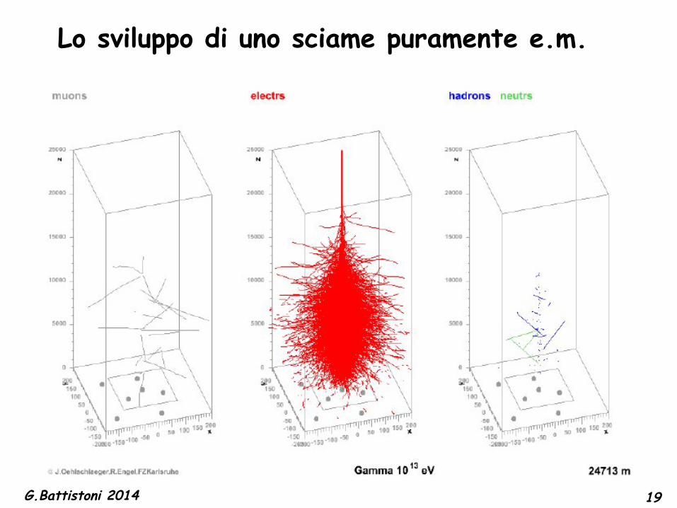
Lo sviluppo di uno sciame puramente e.m.

G.Battistoni 2014 20
Il fronte delle particelle

G.Battistoni 2014 21
il fronte delle particelle 2

G.Battistoni 2014 22
Il fronte delle particelle 3

G.Battistoni 2014 23
P. Auger
Anni 30 e seguenti
C'e' un limite alla dimensione/energia di uno sciame?
Prime osservazioni degli EAS

G.Battistoni 2014 24
Anni '50
Esperimento di Linsley e Scarsi a Volcano Ranch: sembra non esserci limite alla dimensione degli sciami!
Albuquerque

G.Battistoni 2014
25
Il fronte delle particelle 3

G.Battistoni 2014 26
Esperimenti basati a terra per misurare gli sciami prodotti dai raggi cosmici

G.Battistoni 2014 27

G.Battistoni 2014 28
Fronte dello sciame Spessore ~qualche ns
• Dalle differenze dei tempi di arrivo si ricostruisce la direzione di arrivo • Dall’energia deposta in ogni rivelatore si ricava il dNe(X)/dxdy • Dopo integrazione si ottiene Ne(X) • Con l’ausiliio di simulazione da Ne si ottiene E, ma senza informazioni aggiuntive la conversione Ne-E dipende da A

G.Battistoni 2014 29
Spettro dei r.c. e energia degli acceleratori

G.Battistoni 2014 30
Le grandi incertezze delle misure indirette In particolare: la regione del ginocchio

G.Battistoni 2014 31
Misura della composizione: Ne vs Nµ

G.Battistoni 2014 32
Esperimenti di superficie

G.Battistoni 2014 33
Esperimenti di Superficie

G.Battistoni 2014 34
Risultati

G.Battistoni 2014 35

G.Battistoni 2014 36

G.Battistoni 2014 37
La tecnica del Cherenkov atmosferico
Nuova disciplina: la γ-ray astronomy basata a terra
piering
G.Battistoni 2014 38
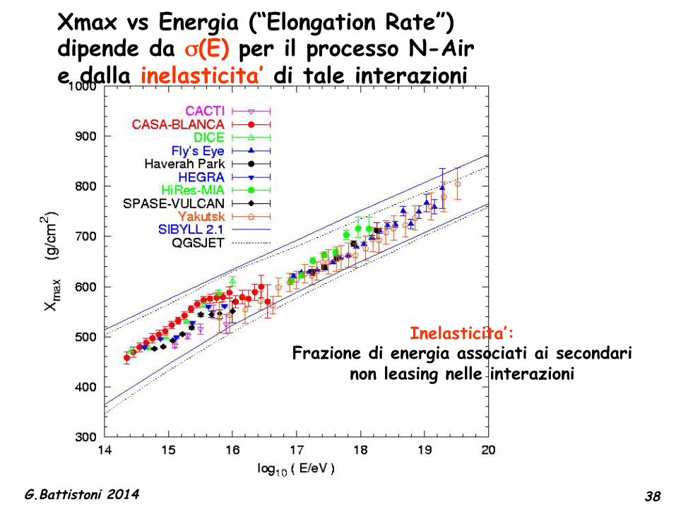
Xmax vs Energia (“Elongation Rate”) dipende da σ(E) per il processo N-Air e dalla inelasticita’ di tale interazioni
Inelasticita’: Frazione di energia associati ai secondari
non leasing nelle interazioni

G.Battistoni 2014 39
Il limite GZK Nel 1966 Greisen e indipendentemente Zatsepin and Kuz’min realizzarono che CMBR doveva limitare la propagazione di protoni ad altissima energia.
GZK cut-off
γ ∈ CMBR ∆(1232 MeV)
M massa del nucleone q momento del γ Eγ = 2.3·10-4 eV
~1020 eV
( / 2)2
(1 cos ) 2(" " )
thrM mE m
qperhead on collisions
ππ
θ
+=
− =
−
Vicino alla soglia la sezione d’urto e’ ~2 10-28 cm2. Per una densita’ di fotoni pari a 400 cm-3 il libero cammino medio viene λ~1025 cm ~ 5 Mpc (tipica dimensione di un cluster di galassie)

Photoproduction of resonances
43
proton (0.938 GeV)
photon
Δ+ resonance (1.232 GeV)proton, neutron
π0, π+
CMB: Energy threshold not sharp
Decay branching ratio proton:neutron = 2:1
Mean proton energy loss 20%
Decay isotropic up to spin effects
In proton rest frame:
E�,lab � 300 MeV
Ep,� =m2
��m2p
2E⇥,max(1� cos⇤)⇥ 1020eV
E�,max ⇥ 10�3eV

Well-established resonances in photoproductionA. Mücke et al. / Computer Physics Communications 124 (2000) 290–314 297
Table 2
Baryon resonances and their physical parameters implemented in SOPHIA (see text). Superscripts + and 0 in the parameters refer to pγ and
nγ excitations, respectively. The maximum cross section, σmax = 4m2NM2σ0/(M2 − m2N)2, is also given for reference
Resonance M Γ 103b+γ σ+
0σ+max 103b0γ σ 0
0σ 0max
$(1232) 1.231 0.11 5.6 31.125 411.988 6.1 33.809 452.226
N(1440) 1.440 0.35 0.5 1.389 7.124 0.3 0.831 4.292
N(1520) 1.515 0.11 4.6 25.567 103.240 4.0 22.170 90.082
N(1535) 1.525 0.10 2.5 6.948 27.244 2.5 6.928 27.334
N(1650) 1.675 0.16 1.0 2.779 7.408 0.0 0.000 0.000
N(1675) 1.675 0.15 0.0 0.000 0.000 0.2 1.663 4.457
N(1680) 1.680 0.125 2.1 17.508 46.143 0.0 0.000 0.000
$(1700) 1.690 0.29 2.0 11.116 28.644 2.0 11.085 28.714
$(1905) 1.895 0.35 0.2 1.667 2.869 0.2 1.663 2.875
$(1950) 1.950 0.30 1.0 11.116 17.433 1.0 11.085 17.462
excitation. The resonances fulfilling these criteria and their parameters, as implemented in SOPHIA after iterative
optimization, are given in Table 2. The phase-space reduction close to the Nπ threshold is heuristically taken into
account by multiplying Eq. (11) with the linear quenching function Qf(ε′;0.152,0.17) for the$(1232)-resonance,
and with Qf(ε′;0.152,0.38) for all other resonances. The function Qf(ε′; ε′th,w) is defined in Appendix 6. The
quenching width w has been determined from comparison with the data of the total pγ cross section, and of the
exclusive channels pπ0, nπ+ and $++π− where most of the resonances contribute. The major hadronic decay
channels of these baryon resonances are Nπ , $π and Nρ; for the N(1535), there is also a strong decay into Nη,
and the N(1650) contributes to the ΛK channel. The hadronic decay branching ratios bc are all well determined
for these resonances and given in the RPP. However, a difficulty arises from the fact that branching ratios can be
expected to be energy dependent because of the different masses of the decay products in different branches. In
SOPHIA, we consider all secondary particles, including hadronic resonances, as particles of a fixed mass. This
implies that, for example, the decay channel $π is energetically forbidden for√
s < m$ + mπ ≈ 1.37 GeV. To
accommodate this problem, we have developed a scheme of energy dependent branching ratios, which change at the
thresholds for additional decay channels and are constant in between. The requirements are that (i) the branching
ratio bc = 0 for ε′ < ε′th,c, and (ii) the average of the branching ratio over energy, weighted with the Breit–Wigner
function, correspond to the average branching ratio given in the RPP for this channel. For all resonances, we
considered not more than three decay channels leading to a unique solution to this scheme. No fits to data are
required. In practice, however, the experimental error on many branching ratios allows for some freedom, which
we have used to generate a scheme that optimizes the agreement with the data on different exclusive channels.
The hadronic branching ratios are given in Table 4 in Appendix 6. To obtain the contribution to a channel with
given particle charges, e.g.,$++π−, the hadronic branching ratio b$π has to be multiplied with the iso-branching
ratios as given in Table 1. We note that with the parameters bγ , bc and biso, the resonant contribution to all exclusive
decay channels is completely determined.
The angular decay distributions for the resonances follow from Eq. (6). In SOPHIA, the kinematics of the decay
channels into Nπ is implemented in full detail (see Table 3). For other decay channels, we assume isotropic
decay according to the phase space. Furthermore, there might be some mixing of the different scattering angular
distributions since the sampled resonance mass, in general, does not coincide with its nominal mass. This effect is
neglected in our work. Instead, we use the angular distributions applying to resonance decay at its nominal massM .
The two decay products of a resonance may also decay subsequently. This decay is simulated to occur
isotropically according to the available phase space.
44
A. Mücke et al. / Computer Physics Communications 124 (2000) 290–314 293
nucleon. For this particle, the Lorentz invariant 4-momentum transfer t = (PN−Pfinal)2 is often used as a final state
variable. At small s, many interaction channels can be reduced to 2-particle final states, for which dσ/dt gives acomplete description.
2.2. Interaction processes
Photon–proton interactions are dominated by resonance production at low energies. The incoming baryon is
excited to a baryonic resonance due to the absorption of the photon. Such resonances have very short life times and
decay immediately into other hadrons. Consequently, the Nγ cross section exhibits a strong energy dependence
with clearly visible resonance peaks. Another process being important at low energy is the incoherent interaction of
photons with the virtual structure of the nucleon. This process is called direct meson production. Eventually, at high
interaction energies (√
s > 2GeV) the total interaction cross section becomes approximately energy-independent,
while the contributions from resonances and the direct interaction channels decrease. In this energy range, photon–
hadron interactions are dominated by inelastic multiparticle production (also called multipion production).
2.2.1. Baryon resonance excitation and decay
The energy range from the photopion threshold energy√
s th ≈ 1.08 GeV for γN -interactions up to√
s ≈ 2 GeV
is dominated by the process of resonant absorption of a photon by the nucleon with the subsequent emission of
particles, i.e. the excitation and decay of baryon resonances. The cross section for the production of a resonance
with angular momentum J is given by the Breit–Wigner formula
σbw(s;M,Γ, J ) = s
(s − m2N)2
4πbγ (2J + 1)sΓ 2
(s − M2)2 + sΓ 2, (4)
whereM and Γ are the nominal mass and the width of the resonance. bγ is the branching ratio for photo-decay of
the resonance, which is identical to the probability of photoexcitation. The decay of baryon resonances is generally
dominated by hadronic channels. The exclusive cross sections for the resonant contribution to a hadronic channel
with branching ratio bc can be written as
σc(s;M,Γ, J ) = bcσbw(s;M,Γ, J ), (5)
with!c bc = 1 − bγ ≈ 1. Most decay channels produce two-particle intermediate or final states, some of them
again involving resonances. For the pion-nucleon decay channel, Nπ , the angular distribution of the final state is
given by
dσNπ
d cosχ∗ ∝J"
λ=−J
###f J1/2,λd
Jλ,1/2(χ
∗)###2
, (6)
where χ∗ denotes the scattering angle in the CMF and f J1/2,λ are the Nπ -helicity amplitudes. The functions
dJλ,1/2(χ
∗) are commonly used angular distribution functions which are defined on the basis of spherical harmonics.TheNπ helicity amplitudes can be determined from the helicity amplitudesA1/2 andA3/2 for photoexcitation (see
Ref. [22] for details), which are measured for many baryon resonances [23]. The same expression applies to other
final states involving a nucleon and an isospin-0 meson (e.g., Nη). For decay channels with other spin parameters,however, the situation is more complex, and we assume for simplicity an isotropic decay of the resonance.
Baryon resonances are distinguished by their isospin into N -resonances (I = 1/2, as for the unexcited nucleon)and (-resonances (I = 3/2). The charge branching ratios biso of the resonance decay follow from isospin
symmetry. For example, the branching ratios for the decay into a two-particle final state involving a N - or (-
baryon and an I = 1 meson (π or ρ) are given in Table 1. Here (I3 is the difference in the isospin 3-componentof the baryon between initial and final state (the baryon charge is QB = I3 + 1/2). In contrast to the strong
decay channels, the electromagnetic excitation of the resonance does not conserve isospin. Hence, the resonance
Breit-Wigner resonance cross section

G.Battistoni 2014 42
3.10 20 eV (Fly’s Eye event)
50 Mpc
p+γ2.7Κ---->p+π0
A+γ2.7Κ---->(A-1)+n
Ancora sul GZK

G.Battistoni 2014 43
La regione delle Energia Estreme
Domande fondamentali • Quale e’ il meccanismo di accelerazione a queste energie? • Quali particelle/nuclei osserviamo? • Quali sono le sorgenti? • Ci sono componenti extra-galattiche? • Esiste il GZK “cutoff” che ci si aspetta? Una finestra verso nuova Fisica Fondamentale

G.Battistoni 2014 44
Esperimenti EHE
AGASA Akeno Giant Air Shower Array
111 scintillatori + 27 riv. muoni
“Classica” analisi basata su Ne vs Nµ
G.Battistoni 2014 45
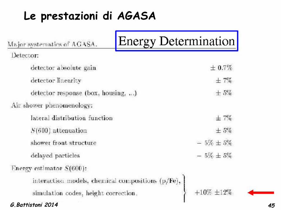
Le prestazioni di AGASA

G.Battistoni 2014 46
Eventi sopra il cutoff GKZ?
11 eventi co E > 1020 eV
errori sistematici di AGASA ~ 18%

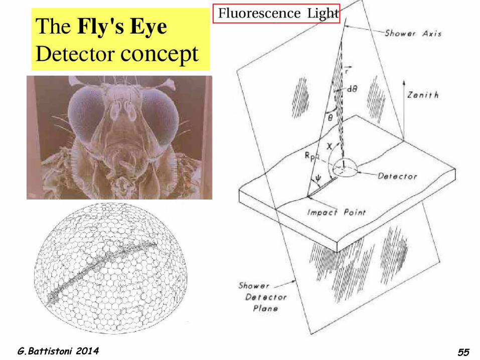
La fluorescenza atmosferica
Un’altra, abbastanza recente, metodologia di osservazione degli EAS è legata al fenomeno della fluorescenza atmosferica: l ’atmosfera terrestre è un enorme scintillatore naturale .
Nel loro passaggio attraverso l’atmosfera, le particelle cariche dello sciame EAS eccitano le molecole d’aria ed in particolare le molecole di azoto in essa presenti; queste , r i tornando a l l oro “stato fondamentale”, emettono luce di fluorescenza nella banda dell’ultravioletto.
L a f l u o r e s c e n z a è e m e s s a isotropicamente e può essere rivelata a grandi distanze dall’asse dello sciame
G.Battistoni 2014 47

… e sue caratteristiche di base Uno sciame EAS prodotto da un cosmico primario di energia
E0>1019 eV forma nell’atmosfera una strisciata di fluorescenza lunga 10-100 km o più, in dipendenza della natura del primario e
dell’angolo di incidenza rispetto alla verticale. E tutto ciò in qualche milionesimo di secondo! Ma la produzione di
fluorescenza è piccola: il suo debole bagliore si può paragonare ad una lampadina UV da pochi Watt che viaggia alla velocità
della luce. Cosa occorre quindi per registrare la luce di fluorescenza ?
• elettronica veloce e molto sensibile • osservazioni notturne senza luna (o quasi)
• cielo sereno (maggior efficienza) • assenza di inquinamento luminoso
Negli array con rivelatori di particelle, viene misurata solo
la distribuzione laterale dello sciame EAS al livello dell’osservazione.
La rivelazione della luce di fluorescenza permette una misura della densità di ionizzazione in un singolo
sciame alle varie altezze e quindi la registrazione dello sviluppo longitudinale dello sciame stesso. G.Battistoni 2014 48

FD
CR
IFD(s)
Ioλ(s) z
CR cosmic ray FD fluorescence detector T transmission function
z altitude
T’s
Y= fluorescence yield in air A = FD acceptance
T= atmospheric transmission function
ε = γ-p.e conversion efficiency R= distance along sight line
≈ 4 photons/m/e
• 10-15 % duty cycle:
clear moonless nights
• clear atmosphere,
no light pollution
300-400 nm light from de-excitation of atmospheric
nitrogen (fluorescence light)
)(4
)()( 2.. λεπ
λλλ
××××=∑i
eep RATYNN
3 0 0 4 0 0 w a v e l e n g t h ( n m )
t i m e
s
Tecnica di fluorescenza
G.Battistoni 2014 49

G.Battistoni 2014 50
La tecnica della misura della luce di fluorescenza

G.Battistoni 2014 51
La tecnica della misura della luce di fluorescenza

G.Battistoni 2014 52

G.Battistoni 2014 53

G.Battistoni 2014 54
G.Battistoni 2014 55

G.Battistoni 2014 56
La luce che raggiunge il PM i-esimo con un angolo di emissione θi arriva con un ritardo rispetto al tempo t0, definito come il tempo al quale il piano del fronte dello sciame passa nel punto piu’ vicino al detector (cioe’ a distanza Rp, ovvero il parametro d’inpatto). Tale ritardo e’ dato da:
,exp 0 tansin tan 2p p p i
ii i
R R Rt t
c c cθ
θ θ− = − =
L’angolo θi dipende dall’angolo di elevazione χi del PM e all’angolo di incidenza ψ dello sciame nel SDP (Shower Detection Plane) secondo la seguente espressione:
i iθ π ψ χ= − −
Il parametro d’impatto Rp, il parametro temporale t0 e l’angolo di incidenza ψ si ottengono dal fit della sequenza temporale dei segnali minimizzando le differenze fra i tempi di arrivo aspettati e misurati:
( )2, ,exp.i meas it t−∑

G.Battistoni 2014 57

G.Battistoni 2014 58

G.Battistoni 2014 59

G.Battistoni 2014 60

G.Battistoni 2014 61
Differenze Hires-Agasa


![[i raggi cosmici]cosmicrays.le.infn.it/Materiale didattico/Altro materiale...4 > 5 asimmetrie 10 / 9.10 / i raggi cosmici La scoperta La storia, anzi la preistoria, dei raggi cosmici](https://img.pdfslide.net/doc/110x75/5c6966b209d3f263648d19dd/i-raggi-cosmici-didatticoaltro-materiale4-5-asimmetrie-10-910-i-raggi.jpg)