1 

Advanced methods in DNA sequence and multilocus data analyses Lesson 1 – DNA sequences I  

I. Sequence editing [BioEdit, MEGA, FaBox, SeqState, R] 

II. Alignment improvement 

III. Model selection [jModeltest, PartitionFinder] 

IV. Tree reconstruction [RAxML, PAUP, MrBayes] 

 

 

I. Sequence editing 

BioEdit software (http://www.mbio.ncsu.edu/BioEdit/bioedit.html).  

As an input you can use simply FASTA format (but also some other formats, as you can check in 

BioEdit).  

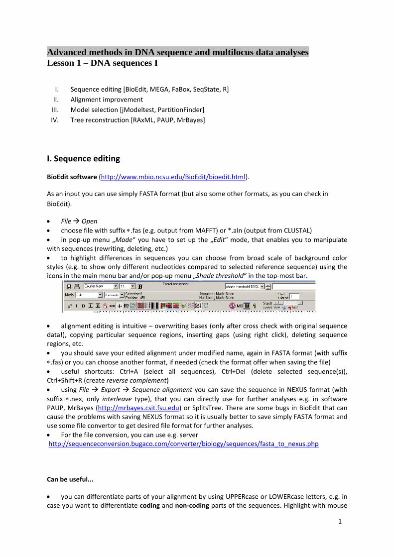
File  Open 

choose file with suffix .fas (e.g. output from MAFFT) or *.aln (output from CLUSTAL) 

in pop‐up menu „Mode“ you have  to set up  the „Edit“ mode,  that enables you  to manipulate with sequences (rewriting, deleting, etc.) 

to  highlight  differences  in  sequences  you  can  choose  from  broad  scale  of  background  color styles (e.g. to show only different nucleotides compared to selected reference sequence) using the icons in the main menu bar and/or pop‐up menu „Shade threshold“ in the top‐most bar. 

 

alignment editing  is  intuitive – overwriting bases (only after cross check with original sequence data!),  copying  particular  sequence  regions,  inserting  gaps  (using  right  click),  deleting  sequence regions, etc. 

you should save your edited alignment under modified name, again in FASTA format (with suffix 

.fas) or you can choose another format, if needed (check the format offer when saving the file) 

useful  shortcuts:  Ctrl+A  (select  all  sequences),  Ctrl+Del  (delete  selected  sequence(s)), Ctrl+Shift+R (create reverse complement)  

using File  Export  Sequence alignment you can save the sequence  in NEXUS  format  (with 

suffix  .nex,  only  interleave  type),  that  you  can  directly  use  for  further  analyses  e.g.  in  software  PAUP, MrBayes (http://mrbayes.csit.fsu.edu) or SplitsTree. There are some bugs  in BioEdit that can cause the problems with saving NEXUS format so it is usually better to save simply FASTA format and use some file convertor to get desired file format for further analyses.  

For the file conversion, you can use e.g. server   http://sequenceconversion.bugaco.com/converter/biology/sequences/fasta_to_nexus.php    Can be useful... 

you can differentiate parts of your alignment by using UPPERcase or LOWERcase letters, e.g. in case you want to differentiate coding and non‐coding parts of the sequences. Highlight with mouse 

  2 

desired  region  of  the  alignment  and  select  in  main  menu  Sequences    Manipulations   UPPERCASE/lowercase 

if you have only coding sequences  in your alignment (e.g. exons)  in correct reading frame, you can  translate  your  nucleotide  sequences  into  aminoacid  sequences  (Ctr+T)  and  estimate  e.g. presence/absence of pseudogenes. 

 

PhyDE software (http://www.phyde.de), for which you need sequences in FASTA or NEXUS 

sequential format. 

File  Open 

select file with suffix .fas  window with alignment appears 

you can move bases or blocks of sequences using mouse – holding  left mouse button highlight desired sequence region, right click, move the sequence block to desired  location, right click again. Editing modes are Align (enables moving the gaps) or Edit (enables editing of sequences). 

File  Export as…  NEXUS (or FASTA, etc.)  

MEGA software (http://www.megasoftware.net/).  

Online manual:  http://www.megasoftware.net/web_help_7/helpfile.htm#hc_first_time_user.htm 

FaBox software (http://users‐birc.au.dk/biopv/php/fabox/) 

using this web tool, you can manipulate fasta format in many different and useful ways. You can e.g. extract (and manipulate) file headers, removing sequences from alignment,  joining alignments, identify haplotypes, convert fasta to other formats etc. 

you can also extract only variable positions from the alignment („Show variable sites only“) 

to create  input  file  for statistical parsimony network analysis  (in TCS) you can use „Create TCS input file from fasta (fasta2tcs)“ 

to  create  input  file  for  MrBayes  you  can  use  „Create  MrBayes  input  file  from  fasta (fasta2mrbayes)“. The file  includes block of commands necessary for MrBayes analysis, but you can also  delete  these  commands  and  use  the  input  file  as  pure  NEXUS  file  for  other  software  (e.g. Splitstree, PAUP etc.).  Converting sequence formats using various web tools:  

 Sequence conversion (http://sequenceconversion.bugaco.com/converter/biology/sequences) 

FormatConverter (http://hcv.lanl.gov/content/sequence/FORMAT_CONVERSION/form.html)  SeaView software (http://doua.prabi.fr/software/seaview)  

Using SeaView you can simply open one of the sequence format you have (FASTA, NEXUS, PHYLIP, etc.) 

File  Save as 

change the type of the output file in the bottom right of the pop‐uped window and save  

SeqState software (http://bioinfweb.info/Software/SeqState). 

  3 

If the alignment includes gaps, i.e.  insertion/deletion (shortly 'indels') that might be phylogenetically informative,  it might  be  necessary  to  code  such  indels  as  additional  characters.    You  can  do  this automatically using  this  software. For  theoretical background, you  should  read e.g. Müller  (2006): Incorporating  information  from  length‐mutational  events  into  phylogenetic  analysis.  Molecular Phylogenetics and Evolution, 38, 667‐676.  Practically: 

File  Load NEXUS file (or Load FASTA file) 

choose file with suffix *.fas or .nex (it have to be sequential format, created e.g. by  PhyDE or reformated using some web tool, see above) 

IndelCoder    simple  indel  coding  (or  another  way  of  coding,  see  the  theoretical  paper mentioned above) 

it creates NEXUS file (in interleave format, and it adds suffix '_mcic.nex' to original file name). In addition to original data matrix the matrix  including coded gaps  is  included. This file can be directly used e.g. in PAUP.  

R software (https://www.r‐project.org/) 

A few simple R scripts to manage molecular data: 

# save sequence names library(phytools) align = read.FASTA(file = "ITS_1.fas")  write.csv(names(align),file="ITS_names.csv") # taky pomocí savelist (seqinr)  # replace sequence names library(seqinr) al <‐ read.fasta(file = "ITS_1.fas") jmena=read.csv(file="ITS_names_new.csv") write.fasta(sequences = al, names = as.vector(jmena$x),              nbchar = 80, file.out = "ITS_1N.fas")  # minimize alignment to a mask library(seqinr) align = read.fasta(file = "Actin_1_MAFFT.fas")  vyber=which(align$mask %in% "1") masked=lapply(align, "[", vyber) write.fasta(sequences = masked, names = names(masked),              nbchar = 80, file.out = "Actin_2_MAFFT.fas")  # minimize alignment to selected sequences library(seqinr) #ITS align_ITS  <‐ read.alignment(file = "ITS_2.fas", format = "fasta") data=read.csv2(file="its‐vyber.csv") vyber_I=match(as.vector(data$ITS),align_ITS$nam) vyber_ITS=vyber_I[!is.na(vyber_I)] write.fasta(sequences = align_ITS$seq[vyber_ITS], names = align_ITS$nam[vyber_ITS],             file.out = "ITS_vyber.fas")  

  4 

# concatenate library(ape) A <‐ read.dna("actin_concat.fas", format="fasta") B <‐ read.dna("ITS_concat.fas", format="fasta") C <‐ cbind(A,B) write.dna(C, "concatenated.fas", format="fasta", colsep="")  

 

II. Alignment improvement 

R script to show the saturation plot  library(ape) data <‐ read.dna("Chlorella_vulgaris.fas", format="fasta") #Convert to genetic distances dist<‐dist.dna(data, model="raw") dist.corrected<‐dist.dna(data, model="TN93") #Make plot plot(dist~dist.corrected,  pch=20,  col="red",  xlab="TrN model  distance",  ylab="Uncorrected  genetic distance", main="Saturation Plot") abline(0,1, lty=2)   

III. Model selection 

Testing  the  models  of  DNA  evolution. Properly  chosen model  of DNA  evolution is  the key  for estimation of  likelihoods of gene  tree  topologies  using  Maximum likelihood and/or Bayesian methods. Before testing models of DNA evolution, it is  important  to  know  the  structure  of analyzed DNA sequence, i.e. what regions represent  coding  sequences, what  region represent non‐coding sequences, etc. The important  step  is  to  realize,  that  some positions  in  alignment  can  evolve  in different  manner  than  the  others,  i.e. under  different  evolutionary  model. Information about  studied  sequence  (and potential  borders  between  coding  and non‐coding  regions)  you  can  found  e.g. using  on‐line  tool  BLAST),  where  the annotations and characteristics of some closely related sequence might be available. The exemplar annotation is shown on the figure on the right.  Since you know the structure of studied region you can partition the dataset into the coding and non‐coding  parts,  i.e.  create  from  single  dataset  two  (or more)  datasets  for which  you  can  estimate proper DNA evolution model separately. You can divide the original dataset 'physically' in BioEdit (or 

  5 

another  alignment  editor)  by  preparing  different  datasets  from  the  original  one  and  saving  them under different names (e.g. '…_exon.fas', '..._intron.fas'). Alternatively, you can add the block of commands into original NEXUS format (or in the separate file), where  the borders of particular  regions are  specified. The  final parts of  the alignments are  called 'partitions'. The  particular  way  of  partition  definition  is  always  better  to  consult  with  documentation  for particular  downstream  analysis  because  the  formats  might  differ  (e.g.  PAUP,  MrBayes, PartitionFInder  etc..).  Exemplar  nexus  block  for  differentiation  of  coding  sequences  according  the position of nucleotides in coding triplets for the purpose of Bayesian analysis is shown below.  begin mrbayes; # začátek nového nexus bloku (může být např. i “Begin sets;”) outgroup 22; charset CHS_pos1 = 1-957\3; # definice úseků - kódující sekvence, první nukleotidy v tripletu charset CHS_pos2 = 2-957\3; # kódující sekvence, druhé nukleotidy v tripletu charset CHS_pos3 = 3-957\3; # kódující sekvence, třetí nukleotidy v tripletu partition Position = 3: CHS_pos1, CHS_pos2, CHS_pos3; # rozdělení datasetu end;  The  DNA  models  for  particular  partitions  you  can  test  using  software  jModeltest (http://code.google.com/p/jmodeltest2/).  The  resulting  models  can  be  than  used  e.g.  for  ML analysis.    Software  jModeltest  do  not  accept  input  datasets  that  are  divided  into  partitions, therefore,  in order to analyze different partitions you have to analyze different parts of the dataset one by one (e.g. separate data file for exons and separate data file for introns).   

File  Load DNA alignment  #  choose file in Nexus or Phylip format  

Analysis  Compute likelihood scores  settings of analysis complexity (i.e. how many different evolutionary models will be tested, from 3 to 88 models). 

If  you  want  to  analyze  your  sequences  with ML,  set  up maximum  number  of models  (I.e. „Number of  substitution  rates“  =  11  and  tick  all  the boxes  for  „Base  frequencies“  and  „Rate variation“). Other settings we can leave as default. 

If  you want  to  analyze  your  sequence  data  using MrBayes,  it  is  enough  to  set  up  only  few selected models, as MrBayes also only allows you to set up only few selected models. For testing the models for MrBayes analysis, you can also use more specific software MrModeltest, that  is in default tests only those models that are further useful for MrBayes analysis. 

Analysis  Do AIC calculation  use default settings and tick the box „write *PAUP block” 

in an output you will find the comparisons of particular models tested and their likelihood scores (the  measure  of  likelihood  of  particular  models  given  your  data).  In  section  „AKAIKE INFORMATION CRITERION (AIC)“ you will find the optimal model for your data selected based on Akaike criterion (AIC). Below you copy set of commands that codes the selected model and  its usage in ML analysis. This commands you can add to the Nexus format with your sequence data.

--

PAUP* Commands Block:

If you want to load the selected model and associated estimates in PAUP*,

attach the next block of commands after the data in your PAUP file:

[!

Likelihood settings from best-fit model (HKY+G) selected by AIC

with jModeltest 0.1.1 on Thu Oct 17 13:26:26 CEST 2013]

BEGIN PAUP;

Lset base=(0.4010 0.2062 0.1059 0.2870) nst=2 tratio=3.3506 rates=gamma shape=0.4330 ncat=4

pinvar=0;

END;

-- 

  6 

 Alternatively, you can test DNA models and simultaneously find the best partition for you data using PartitionFinder  (http://www.robertlanfear.com/partitionfinder/).  We  will  describe  its  usage  for further ML  analysis  of  your  data.  The  advantage  of  this  approach  is  the  possibility  to  load  single dataset  that  can  be  divided  into  the  partitions  (as  described  above).  Software  then  test  all DNA models  for  all  partitions  and  further  decide,  which  partitions  should  use  different  evolutionary models  and  potentially  also  which  partitions  can  be  described  by  the  evolutionary  model  and therefore can be joined together. This is especially useful when we want to know, if it's necessary to differentiate  in our DNA region only exons and  introns or  if we want to differentiate also different positions within  the  coding  regions.  In  the  latter  case  you  usually  end  up with more  than  three partitions  so  it  is  more  practical  to  use  PartitionFinder  for  model  testing  in  such  a  cases. PartitionFinder  is  the python script so  in order  to  run  it, you have  to have  the Python  installed on your computer (see http://www.python.org/).   

There  are  two  input  files  that  should  be  located  in  the  single  folder  ‐  the  file  including  your alignment in Phylip format and the configuration file „partition_finder.cfg“ in which you specify the name of the input sequence file (*.phy), define the partitions of your dataset and select the way of model testing. When editing the *.cfg file it is better to check the original documentation that comes with PartitionFinder. Default/exemplar setting can be like this: 

 ## ALIGNMENT FILE ## alignment = test.phy; ## BRANCHLENGTHS: linked | unlinked ## branchlengths = linked; ## MODELS OF EVOLUTION for PartitionFinder: all | raxml | mrbayes | beast | <list> ## ## for PartitionFinderProtein: all_protein | <list> ## models = all; # MODEL SELECCTION: AIC | AICc | BIC # model_selection = BIC; ## DATA BLOCKS: see manual for how to define ## [data_blocks] Gene1_pos1 = 1-1062\3; Gene1_pos2 = 2-1062\3; Gene1_pos3 = 3-1062\3; ## SCHEMES, search: all | greedy | rcluster | hcluster | user ## [schemes] search = greedy; #user schemes go here if search=user. See manual for how to define.#

You run analysis from the command line. In Windows you can call the command line using Start  Run  cmd  

In the command line, you write command of following structure: python ”<PartitionFinder.py>” “<inputFolderName>” 

where  ”<PartitionFinder.py>”  is  the PATH  to  the python  script PartitionFinder.py  (that  can be wherever  in the computer) and “<inputFolderName>” that represents PATH to the folder with input files (it also can be locate wherever). Both PATH you can import to the command line after command “python” by mouse drag and drop. 

 

After the end of analysis the new folder with name „analysis“ appears in your working directory. In  this  folder you will be mainly  interested  in  file “best_schemes.txt”, where you will  find  the information about the best option for grouping of particular partitions into the groups with the same model of evolution.  

Subset | Best Model | Subset Partitions| Subset Sites | Alignment

  7 

1 | F81+G | Gene1_pos1, Gene2_pos1, Gene3_pos1 | 1-789\3, 790-1449\3, 1450-2208\3 | ..... 2 | F81+G | Gene1_pos2, Gene2_pos2, Gene3_pos2 | 2-789\3, 791-1449\3, 1451-2208\3 | ..... 3 | K80+G | Gene1_pos3 | 3-789\3 | ..... 4 | TrN+G | Gene2_pos3, Gene3_pos3 | 792-1449\3, 1452-2208\3 | .... Scheme Description in PartitionFinder format Scheme_step_5 = (Gene1_pos1, Gene2_pos1, Gene3_pos1) (Gene1_pos2, Gene2_pos2, Gene3_pos2) (Gene1_pos3) (Gene2_pos3, Gene3_pos3);  

The software, however, do not generate Nexus block of commands  that you could directly paste  into  your  alignment  file.  You  have  to  create  this  block  by  yourself  based  on  the information from the file „best_schemes.txt”.  

 

IV. Tree reconstruction 

Fast construction of ML tree and other useful analyses in MEGA  Software MEGA can be useful from several points of view. You can view your alignment and convert FASTA file into other sequence formats (e.g. NEXUS, PHYLIP), test your sequence data if they evolve according molecular  clocks or  construct ML  tree  in  rather  fast way. We  recommend  to use other software for serious ML reconstruction for your final datasets (e.g. RaxML, Garli), however, you can use MEGA for the first insight into your data. 

 

Fast construction of ML tree 

o open Fasta alignment in MEGA 

o Phylogeny – Construct/Test Maximum LikelihoodTree: 

Test ofPhylogeny – none (or you can choose here if you want to use 

Bootstrap analysis to estimate reliability of your gene topology)  

Substitution Model &RatesamongSites – choose suitable DNA evolution 

model according previous jModeltest (or another) analysis 

Compute 

o After the end of analysis final tree appears. You can save it using: File – Export 

CurrentTree (Newick)  

Format conversion 

o open Fasta alignment in MEGA 

o Data → Explore active data. Your alignment appears in new window. In this active 

window, it is better to click and deactivate the icon 'Use identical symbol' to see 

particular nucleotides in the alignment. 

o Data → Export data 

o in section 'Format' choose the desired format for export and click 'OK'. You can also 

check some other options for the export, if needed. 

 

Test dataset for molecular clocks 

o open Fasta alignment in MEGA 

o Clocks → Test Molecular Clocks (ML)  

o You have to specify the tree topology for your data in the section 'Tree to Use' using 

'Use tree from file' and then navigate the software to the directory where you store 

your tree (e.g. in newick format) 

  8 

o You should specify the evolutionary model for your data in section 'Model/Method' 

o other settings you can leave as it is by defaults and run analysis using 'Compute' 

o After the end of analysis the new window will appear with all the information  

Construction  of  a  ML  tree  using  RAxML  (http://sco.h‐its.org/exelixis/web/software/raxml/index.html) Python version: http://sourceforge.net/projects/raxmlgui/ 

Windows version: https://github.com/stamatak/standard‐

RAxML/tree/master/WindowsExecutables_v8.1.20 

 

Basic parameters 

‐m  specification of substitution model 

‐p  random seed 

‐t  starting tree (if not specified, a parsimony tree is automatically created) 

‐s  name of input file (in phylip format) 

‐#  number of replications 

‐n  name appendix of resulting files 

 

1. ML on binary data 

raxmlHPC ‐m BINGAMMA ‐p 12345 ‐s binary.phy ‐# 20 ‐n resultBIN 

‐ using GAMMA model 

‐ 20 replications 

 

2. ML on DNA data 

raxmlHPC ‐m GTRGAMMA ‐p 12345 ‐s dna.phy ‐# 20 ‐n resultDNA 

 

3. bootstrapping 

a) first a best‐scoring ML tree is found 

raxmlHPC ‐m GTRGAMMA ‐p 12345 ‐# 20 ‐s dna.phy ‐n bestML 

b) a bootstrap analysis is followed 

raxmlHPC ‐m GTRGAMMA ‐p 12345 ‐b 12345 ‐# 100 ‐s dna.phy ‐n boot 

‐ bootstrap trees are generated to RAxML_bootstrap.boot 

c) bootstrap values are mapped on the best‐scoring ML tree 

raxmlHPC ‐m GTRGAMMA ‐p 12345 ‐f b ‐t RAxML_bestTree.bestML ‐z RAxML_bootstrap.boot ‐n 

finalboot 

‐ RAxML_bipartitions.finalboot file (bootstrap values as nodes) and 

RAxML_bipartitionsBranchLabels.finalboot file (bootstrap values on branches)  

4. rapid bootstrapping 

‐ complete analysis in one step(ML search+ bootstrapping): 

raxmlHPC ‐f a ‐m GTRGAMMA ‐p 12345 ‐x 12345 ‐# 100 ‐s dna.phy ‐n rbs 

‐ RAxML_bipartitions.rbs file is created – the best ML tree with bootstrap values mapped 

Construct a MP tree using PAUP 

 

Open a file: 

1. File ‐> Open… (select a NEXUS file) 

or File ‐> Import Data … (can open FASTA, PHYLIP, etc.) 

  9 

2. File ‐> Execute (or CTRL + R) 

3. File ‐> Log Output To Disk 

 

Perform a ML analysis: 

1. Analysis ‐> Parsimony 

2. Analysis ‐> Parsimony Settings… 

Optimization – ACCTRAN or DELTRAN 

Gaps – Missing Data 

3. Analysis ‐> Heuristic Search 

General: Keep – optimal trees only, Set MaxTrees – 1000, Leave unchanged 

Starting trees – Get by stepwise addition 

Stepwise addition: Addition sequence – random, # reps – 10 

Branch swapping: swapping algorithm – TBR 

4. Trees ‐ > Root Trees… 

Rooting Options… ‐ Define Outgroup… ‐ click to outgroup species 

5. Trees ‐> Print/View Trees… 

6. Trees ‐> Compute Consensus… ‐ Strict, Majority‐rule (50%), Include values in treefile… as node 

labels, Output to treefile 

7. Trees ‐> Print/View Consensus Tree(s)… 

 

Bootstrapping: 

1. Analysis ‐> Bootstrap/Jackknife Analysis 

Resampling method – Bootstrap 

Number of replicates 

2. Trees ‐> Print/View Bootstrap Consensus… 

 

Construct a Bayesian tree using MrBayes (http://mrbayes.sourceforge.net/) 

 

test alignments: 

o test.nex – concatenated dataset 

Bayesian inference o a MrBayes block is added at the end of Nexus file: 

  

begin mrbayes; charset 18S = 1‐1782; charset psa = 1783‐2702; charset cox = 2703‐3285; partition marker = 3:18S,psa,cox;   set partition = marker;  prset applyto=(all) ratepr=variable;   lset applyto=(1)   nst=6  rates=invgamma; lset applyto=(2)   nst=6  rates=propinv; lset applyto=(3)   nst=2  rates=equal; 

‐ 1st partition definition 2nd partition definition 3rd partition definition partitioning definition set partitions  priors definition (partitions are given in brackets); 

ratepr=variable: partitions may have different evolutionary rates   

substitution models definition (partitions in brackets, again); nst=1 (JC, F81), nst=2 (K80, HKY), nst=6 (GTR); rates=equal / gamma (Γ) / propinv (I) 

  10

    unlink statefreq=(all) revmat=(all) tratio=(all) shape=(all) pinvar=(all);    mcmc ngen=5000000 samplefreq=100 relburnin=no;  end; 

/invgamma (Γ + I)  each partition may have unique parameters of 

substitution models    set a mcmc analysis: ngen=number of generations; 

samplefreq=rate of writing parameters into files 

    

o in addition to the above‐mentioned parameters, the analysis is based on several default parameters. Their values can be listed by typing „help“:  help prset = list of priors  help lset = list of model parameters  help mcmc = list of mcmc parameters 

o Bayesian analysis is run by typing „mrbayes“ and „exe FILENAME.nex“ 

analysis evaluation o at the end of analysis, MrBayes asks asks whether or not you want to continue with 

the analysis. Before answering that question, examine the average standard deviation of split frequencies. If the value is higher than 0.05, the analysis should be prolonged. Values less than 0.01 indicate a good convergence. 

drawing a consensus tree:  

sump    ‐or‐  sump relburnin=no burninfrac=0.1  sumt contype=allcompat  ‐or‐  sumt relburnin=no burninfrac=0.1 contype=allcompat   

summary of model parameters.   Burnin = number of discarded generations. Should be set to obtain 

a stationary phase (a graph includes randomly placed letters 1, 2 and *) – see the picture below. If only “sump” is typed, a 25% of generations are discarded. To set the burnin value manually, “relburnin=no“ should be typed. 

   creating a consensus tree, setting a burnin parameter as indicated 

above. “contype=allcompat“ returns a fully bifurcated tree. 

 Ideal sumt result If the numbers are not intermixed, or If you see an obvious trend in the plot, either increasing or decreasing, the analysis should be run longer. Finally, the values of PSRF+ parameters should be checked. The values should be close to 1.00.     

  11

 results of you analysis.