IAB Discussion Paper 44/2008doku.iab.de/discussionpapers/2008/dp4408.pdf · We treat this problem as a missing data problem and derive new multiple imputation approaches to impute

IAB Discussion Paper 44/2008

Thomas Büttner Susanne Rässler

Multiple Imputation of Right-Censored Wages in the German IAB Employment Sample Considering Heteroscedasticity

Articles on scientific dialoge

Multiple Imputation of Right-Censored Wages

in the German IAB Employment Sample

Considering Heteroscedasticity

Thomas Büttner (IAB)

Susanne Rässler (Otto-Friedrich-Universität Bamberg)

Mit der Reihe „IAB-Discussion Paper“ will das Forschungsinstitut der Bundesagentur für Arbeit den

Dialog mit der externen Wissenschaft intensivieren. Durch die rasche Verbreitung von Forschungsergebnissen

über das Internet soll noch vor Drucklegung Kritik angeregt und Qualität gesichert werden.

The “IAB Discussion Paper” is published by the research institute of the German Federal Employ-

ment Agency in order to intensify the dialogue with the scientific community. The prompt publication

of the latest research results via the internet intends to stimulate criticism and to ensure research

quality at an early stage before printing.

IAB-Discussion Paper 44/2008 2

Contents

Abstract 4

1 Introduction 5

2 Imputation approaches for censored wages 62.1 Homoscedastic imputation approaches . . . . . . . . . . . . . . . . . . . . 7

2.1.1 Homoscedastic single imputation . . . . . . . . . . . . . . . . . . . 72.1.2 Multiple imputation assuming homoscedasticity . . . . . . . . . . . 7

2.2 Heteroscedastic imputation approaches . . . . . . . . . . . . . . . . . . . . 92.2.1 Heteroscedastic single imputation . . . . . . . . . . . . . . . . . . . 92.2.2 Multiple imputation considering heteroscedasticity . . . . . . . . . . 9

3 Simulation study 113.1 The IAB employment sample . . . . . . . . . . . . . . . . . . . . . . . . . . 113.2 Creating a complete population . . . . . . . . . . . . . . . . . . . . . . . . 123.3 Simulation design . . . . . . . . . . . . . . . . . . . . . . . . . . . . . . . 12

4 Results 154.1 Homoscedastic data set . . . . . . . . . . . . . . . . . . . . . . . . . . . . 154.2 Heteroscedastic data set . . . . . . . . . . . . . . . . . . . . . . . . . . . . 16

5 Conclusion 16

6 References 20


Abstract

In many large data sets of economic interest, some variables, as wages, are top-coded

or right-censored. In order to analyze wages with the German IAB employment sample

we first have to solve the problem of censored wages at the upper limit of the social se-

curity system. We treat this problem as a missing data problem and derive new multiple

imputation approaches to impute the censored wages by draws of a random variable from

a truncated distribution based on Markov chain Monte Carlo techniques. In general, the

variation of income is smaller in lower wage categories than in higher categories and the

assumption of homoscedasticity in an imputation model is highly questionable. Therefore,

we suggest a new multiple imputation method which does not presume homoscedasticity of

the residuals. Finally, in a simulation study, different imputation approaches are compared

under different situations and the necessity as well as the validity of the new approach is

confirmed.

JEL classification: C24, C15

Keywords:

top coding, missing data, censored wage data, Markov chain Monte Carlo

Acknowledgements: The authors thank Hermann Gartner, Hans Kiesl and Johannes

Ludsteck for their support and helpful hints. Of course, all remaining errors are ours.


1 Introduction

For a large number of research questions, like analyzing the gender wage gap or measur-

ing overeducation with earnings frontiers, it is interesting to use wage data. To address this

kind of questions two types of data are usually used: surveys and process generated data,

i.e. administrative data. Administrative data have several advantages, like a large number

of observations, no nonresponse burden and no problems with interviewer effects or survey

bias. Unfortunately, in many large administrative data sets of economic interest some vari-

ables, such as wages, are top-coded or right-censored. This problem is very common with

administrative data from social security systems like the IAB employment sample (IABS),

which is based on the register data of the German social insurance system. The contribu-

tion rate of this insurance is charged as a percentage of the gross wage. Is the gross wage

higher than the current contribution limit, however only the amount of the ceiling is liable

for the contribution. In 2008 the contribution limit in the unemployment insurance system

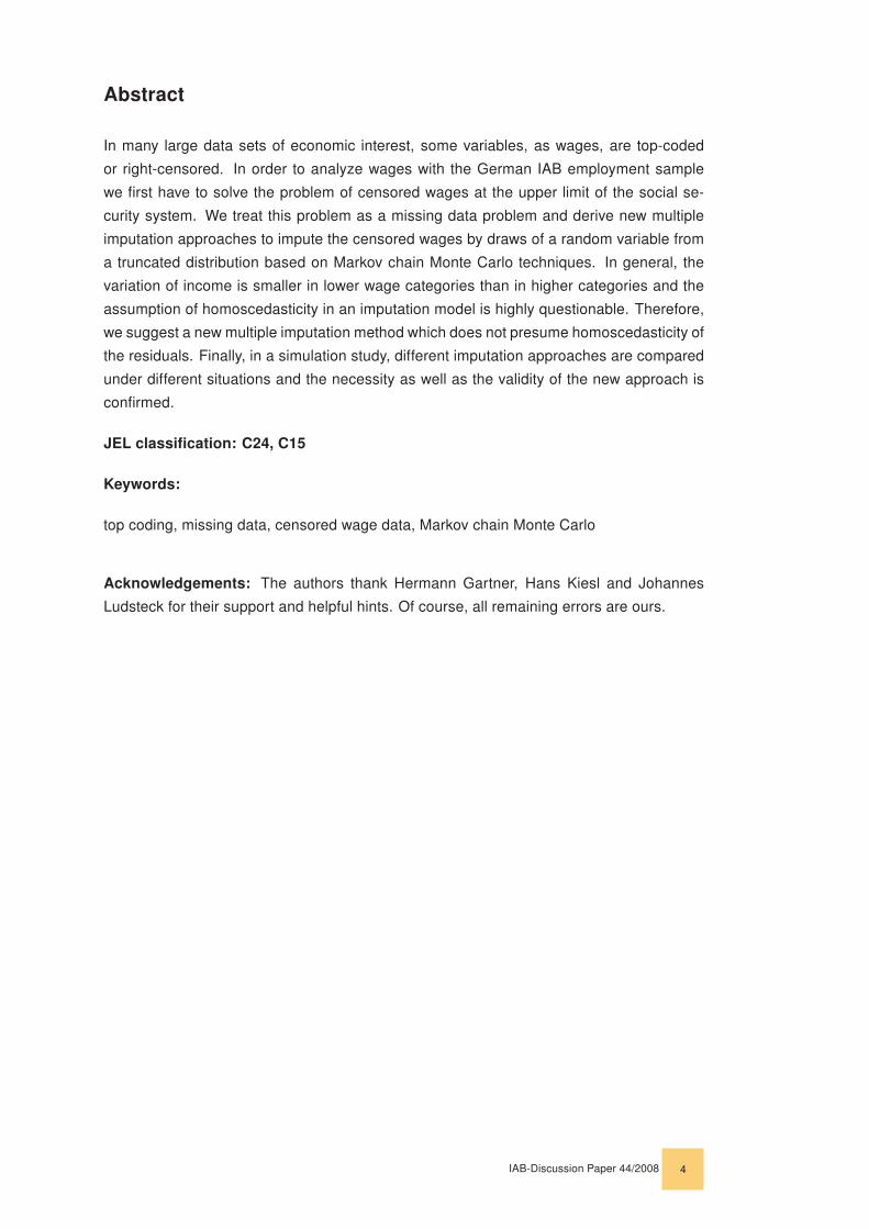
is fixed in Western Germany at a monthly income of 5,300 euros. As therefore wages are

only recorded up to this contribution limit, the wage information in this sample is censored

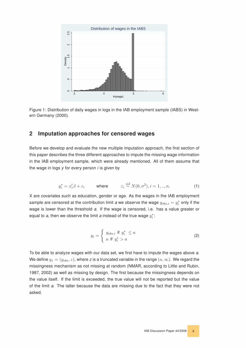
at this limit. (Figure 1 shows the distribution of wages in the IAB employment sample in

2000).

In order to analyze wages with the IAB employment sample, we first have to solve the prob-

lem of the censored wages (see Rässler 2006). We treat this problem as a missing data

problem and use imputation approaches to impute the censored wages. Gartner (2005)

proposes a non-Bayesian single imputation approach to solve the problem of the censored

wages. Another approach - a multiple imputation method based on draws of a random vari-

able from a truncated distribution and Markov chain Monte Carlo techniques - is suggested

by Gartner and Rässler (2005). These two approaches assume homoscedasticity of the

residuals. But on the contrary of this assumption, the variance of income is smaller in lower

wage categories than in higher categories and assuming homoscedasticity in an imputation

model is highly questionable. Thus, in a first step, we develop a third approach, a second

single imputation approach based on GLS estimation to consider heteroscedasticity.

First results of a simulation study using these three methods show the necessity to develop

another method that imputes the missing wage information multiply and does not assume

homoscedasticity. Therefore, we suggest a new multiple imputation method allowing for

heteroscedasticity and finally compare in a simulation study the four different imputation

approaches again under different situations using a sample of the IAB employment sample

in order to confirm the superiority of the new approach.

The paper is organized as follows: The next section describes the four different imputation

approaches. The section starts with the imputation approaches assuming homoscedastic-

ity and continues with the new imputation approaches considering heteroscedasticity. In

Section 3 we provide a description of the simulation study, followed by the results in Section

4. Finally, Section 5 concludes.


0.5

11.

52

2.5

Den

sity

3 4 5 6ln(wage)

Distribution of wages in the IABS

Figure 1: Distribution of daily wages in logs in the IAB employment sample (IABS) in West-ern Germany (2000).

2 Imputation approaches for censored wages

Before we develop and evaluate the new multiple imputation approach, the first section of

this paper describes the three different approaches to impute the missing wage information

in the IAB employment sample, which were already mentioned. All of them assume that

the wage in logs y for every person i is given by

y∗i = x′iβ + εi where εiiid∼ N(0, σ2), i = 1, .., n. (1)

X are covariates such as education, gender or age. As the wages in the IAB employment

sample are censored at the contribution limit a we observe the wage yobs,i = y∗i only if the

wage is lower than the threshold a. If the wage is censored, i.e. has a value greater or

equal to a, then we observe the limit a instead of the true wage y∗i :

yi =

{yobs,i if y∗i ≤ a

a if y∗i > a(2)

To be able to analyze wages with our data set, we first have to impute the wages above a.

We define yz = (yobs, z), where z is a truncated variable in the range (a,∞). We regard the

missingness mechanism as not missing at random (NMAR, according to Little and Rubin,

1987, 2002) as well as missing by design. The first because the missingness depends on

the value itself. If the limit is exceeded, the true value will not be reported but the value

of the limit a. The latter because the data are missing due to the fact that they were not

asked.


2.1 Homoscedastic imputation approaches

2.1.1 Homoscedastic single imputation

One possibility to impute the missing wage information is using a single imputation ap-

proach. A homoscedastic single imputation based on a tobit model is proposed by Gartner

(2005). A tobit model (see Greene 2008) is used to estimate the parameter β and σ2 of the

imputation model. According to the estimated parameters the censored wage z can be im-

puted by draws of a random value. As we know that the true value is above the contribution

limit we have to draw a random variable from a truncated normal distribution

zi ∼ Ntrunca(x′iβ̂, σ̂2) if yi = a for i = 1, ..., n. (3)

This means we add to the expected wage an error term ε (see Gartner 2005).

zi = x′iβ̂ + εi if yi = a for i = 1, ..., n (4)

Using a single imputation approach, we have to consider that this method may lead to bi-

ased variance estimations. Thus, Little and Rubin (1987, 2002) suggest that imputation

should rather be done in a multiple and Bayesian way according to Rubin (1978). There-

fore, we better use multiple imputation approaches to impute the missing wage information.

Multiple imputation is discussed in detail in Rubin (1987, 2004a, 2004b) or Rässler et al.

(2007). For computational guidance on creating multiple imputations see Schafer (1997).

2.1.2 Multiple imputation assuming homoscedasticity

To start with, let Y = (Yobs, Ymis) denote the random variables concerning the data with

observed and missing parts. In our specific situation this means that for all units with

wages below the limit a each data record is complete, i.e., Y = (Yobs) = (X,wage). For

every unit with a value of the limit a for its wage information we treat the data record as

partly missing, i.e., Y = (Yobs, Ymis) = (X, ?). X is observed for all units. Thus, we have

to multiply impute the missing data Ymis = wage. The theory and principle of multiple

imputation originates from Rubin (1978) and is based on independent random draws from

the posterior predictive distribution fYmis|Yobsof the missing data given the observed data.

As it may be difficult to draw from fYmis|Yobsdirectly, a two-step procedure for each of the

m draws is useful:

(a) First, we perform random draws of Ξ according to the observed-data posterior distribu-

tion fΞ|Yobs, where Ξ is the parameter vector of the imputation model.

(b) Then, we make random draws of Ymis according to their conditional predictive distribu-

tion fYmis|Yobs,Ξ.


Because

fYmis|Yobs(ymis|yobs) =

∫fYmis|Yobs,Ξ(ymis|yobs,ξ)fΞ|Yobs

(ξ|yobs)dξ (5)

holds, with (a) and (b) we achieve imputations of Ymis from their posterior predictive dis-

tribution fYmis|Yobs. Due to the data generating model being used, for many models the

conditional predictive distribution fYmis|Yobs,Ξ is rather straightforward. That means it can

be more or less easily formulated for each unit with missing data. In contrast, the corre-

sponding observed-data posteriors fΞ|Yobsare usually difficult to derive for those units with

missing data, especially when the data have a multivariate structure. In these cases, they

often do not follow a standard distribution from which random numbers can easily be gener-

ated. However, simpler methods have been developed to enable multiple imputation based

on Markov chain Monte Carlo (MCMC) techniques (Schafer 1997). In MCMC the desired

distributions fYmis|Yobsand fΞ|Yobs

are achieved as stationary distributions of Markov chains

based on the complete-data distributions, which are easier to compute.

Imputation model

Gartner and Rässler (2005) suggest an imputation approach based on Markov chain Monte

Carlo techniques to multiply impute the right-censored wages in the IAB employment sam-

ple, which contains the following steps. To be able to start the imputation based on MCMC,

we first need to adapt starting values for β(0) and the variance σ2(0) from a ML tobit esti-

mation. Second, in the imputation step, values for the missing wages are randomly drawn

from the truncated distribution in analogy to the single imputation procedure

z(t)i ∼ Ntrunca(x

′iβ

(t), σ2(t)) if yi = a for i = 1, ..., n. (6)

Then an OLS regression is computed based on the imputed data according to

β̂(t)z = (X ′X)−1X ′y(t)

z . (7)

After this step, new random draws for the parameters can be produced according to their

complete data posterior distribution. To draw the variance σ2(t+1) we need the inverse of a

gamma distribution, which is produced as follows:

g ∼ χ2(n− k) (8)

σ−2(t+1) =g

RSS(9)


where RSS is the residual sum of squares RSS =n∑

i=1(y(t)

zi − x′iβ̂(t)z )2 and k is the number

of columns of X.

Now new random draws for the parameter β can be performed

β(t+1)|σ2(t+1) ∼ N(β̂(t)z , σ2(t+1)(X ′X)−1). (10)

We repeat the imputation and the posterior-steps (6) to (10) 6,000 times and use (z2000i , z3000

i , . . . , z6000i )

to obtain 5 complete data sets. For more details see Gartner and Rässler (2005) or Jensen

et al. (2006).

2.2 Heteroscedastic imputation approaches

2.2.1 Heteroscedastic single imputation

As we assume that the variation of income is smaller in lower wage categories than in

higher categories, we suppose an imputation approach considering heteroscedasticity.

Therefore we first use another single imputation procedure based on the first single im-

putation approach, a method that does not presume homoscedasticity of the residuals.

We assume that the error variance is related to a number of exogenous variables, gathered

in a vector w (not including a constant). We use a GLS model for truncated variables

(e.g. intreg in STATA) to estimate the parameters of the imputation model, β, like in the

first approach, and furthermore γ, describing the functional form of the heteroscedasticity.

Then the imputation can be done by draws from a truncated normal distribution, similar to

the first approach,

zi ∼ Ntrunca(x′iβ̂, σ̂2

i ) where σ̂2i = ew′iγ̂ if yi = a for i = 1, ..., n, (11)

where w is a vector of observed variables that is a function of x, e.g subset of x vari-

ables. To consider the heteroscedastic structure of the residuals, we use here individual

variances for every person to draw a random value. This solution takes into consideration

the existence of heteroscedasticity, yet it does not solve the problem of biased variance

estimations. Therefore, we have to derive the Bayesian solution.

2.2.2 Multiple imputation considering heteroscedasticity

Since we assume the necessity of an approach that does not presume homoscedasticity

and since Little and Rubin (1987, 2002) among others show that single imputation ap-

proaches may lead to biased variance estimations, consequently we suggest a new mul-

tiple imputation approach. A first simulation study using the first three approaches shows


as well the need for this approach. This simulation study points out that, in case of a ho-

moscedastic structure of the residuals, the multiple imputation leads to better results than

a single imputation approach. But in case of heteroscedasticity the single imputation con-

sidering heteroscedasticity is superior to the multiple imputation approach suggested by

Gartner and Rässler (2005). This indicates the necessity to develop another approach that

combines these two properties: an approach performing multiple imputation and consider-

ing heteroscedasticity.

Imputation model

We develop this new method based on the multiple imputation approach proposed by Gart-

ner and Rässler (2005). The basic element of the new approach is that we need additional

draws for the parameters γ describing the heteroscedasticity. We start now the imputation

by adapting starting values for β(0) and γ(0) from a GLS estimation for truncated variables

like in the heteroscedastic single imputation approach. Then we are able to draw values

for the missing wages from a truncated distribution using individual variances σ2i = ew′iγ

again like in the heteroscedastic single imputation model:

z(t)i ∼ Ntrunca(x

′iβ

(t), σ2(t)i ) where σ

2(t)i = ew′iγ

(t)if yi = a for i = 1, ..., n. (12)

Then a GLS regression is computed based on the imputed data set (comparable to the

OLS regression in the homoscedastic multiple imputation approach) to obtain β̂(t)z and γ̂(t).

Additionally we estimate V (γ̂(t)) to be able to perform the following steps. Afterwards we

produce new random draws for the parameters according to their complete data posterior

distribution. As we consider now the existence of heteroscedasticity, some modifications

of the algorithm are necessary. In the first step, we draw the variance σ2(t+1) according to

g ∼ χ2(n− k) (13)

σ−2(t+1) =g

RSS(14)

where

RSS =n∑

i=1

exp(ln ε̂2i − w′iγ̂

(t)) =n∑

i=1

(y(t)zi − x′iβ̂

(t))2

ew′iγ̂(t). (15)

In an additional step, we have to perform random draws for γ

γ(t+1) ∼ N(γ̂(t), V̂ (γ̂(t))) (16)


Consequently the parameters β can be drawn like in the Gartner and Rässler approach,

again with a slight modification compared to the homoscedastic multiple imputation:

β(t+1)|γ(t+1), σ2(t+1) ∼ N(β̂(t)z , σ2(t+1)(

n∑

i=1

xix′i

ew′iγ(t+1))−1). (17)

Again, we repeat the steps (12) to (17) 6,000 times and use (z2000i , z3000

i , . . . , z6000i ) to

obtain the 5 complete data sets.

3 Simulation study

To evaluate the results delivered by these different approaches under different situations

in order to show the relevance of the suggested multiple imputation approach, we perform

a simulation study using the IAB employment sample. We first create a complete data

set without censored wages, define a new limit and delete the wages above this limit.

Afterwards, the missing wages are imputed using the different approaches and the results

are compared to the complete data set.

3.1 The IAB employment sample

The German IAB employment sample (IABS) is a 2 percent random sample drawn from

the IAB employee history with additional information on benefit recipients and hence is a

sample of all employees covered by social security. Consequently self-employed, family

workers and civil servants are not included. The data set represents approximately 80 per-

cent of all employees in Germany. The IABS includes, among others, information on age,

sex, education, wage and the occupational group. For the sample two sources of data are

combined: Information on employment coming from employer reports to the social secu-

rity and information about unemployment compensation coming from the German federal

employment agency. As already mentioned, the wage information in the IABS is censored

at the contribution limit of the unemployment insurance. For further insight on the data set

see Bender et al.(2000).

To simplify the simulation design, we restrict the data for the simulation to male West-

German residents. We use all workers holding a full-time job covered by social security

effective on June 30th 2000. The data set contains 214,533 persons: 23,685 or 11 percent

of them with censored wages. The following table shows descriptive information about

the fraction of censored incomes of six educational and five age groups to demonstrate

the need to impute the missing wage information. Especially for analyzing highly-skilled

employees (with technical college degree or university degree) the table indicates the ne-

cessity to impute the missing wages.


<25 25-34 35-44 45-54 55+Low/intermed. school 0 .003 .008 .012 .17Vocational training .001 .021 .068 .116 .150Upper school .010 .110 .232 .331 .371Upper school

and vocational training .003 .110 .283 .393 .470Technical college .024 .190 .450 .558 .604University degree .056 .256 .549 .686 .769

Table 1: Fractions of censored wages in the original data set

For the simulation study we assume a model containing the wages in logs as dependent

variable and age, squared age, nationality as well as dummies for six education levels and

four categories of job level as independent variables.

3.2 Creating a complete population

To perform the simulation study, a complete population is created in order to be able to

compare the results of the different approaches with a complete data base. As the wage

information in our sample is right-censored, we first have to impute our sample to obtain

this control population. The fact that the data set has to be imputed before starting the

simulation study allows us to produce control populations with different characteristics: We

create one data set where homoscedasticity is existent and another with heteroscedasticity

of the residuals. To obtain the first data set (data set A) we use the homoscedastic single

imputation procedure as described in section 2.1.1 to impute new wages for every person

regardless if the wage was originally censored or not, according to

ynew ∼ N(x′β̂, σ̂2), (18)

again with β̂ and σ̂2 from a tobit estimation based on the right-censored sample. To receive

the second data set (data set B), the heteroscedastic single imputation method described

in section 2.2.1 is used in order to receive a control population with heteroscedasticity of

the residuals, according to

ynew ∼ N(x′β̂, σ̂2i ). (19)

These two data sets will later be used as complete populations for the analysis of the

results we receive by using the different approaches.

3.3 Simulation design

The simulation study consists of four steps. Each of these steps is simultaneously done for

the homoscedastic data set A and the heteroscedastic population B: We draw random sam-


ples from the complete population repeatedly, define the threshold and impute the wage

above this threshold using the four approaches. Then we compare the imputed data sets

with the complete population.

Step 1: Drawing of a random sample

In the first step a random sample of n=21,453 persons is drawn without replacement from

the population of N=214,533 persons (equivalent to 10 percent). This 10 percent random

sample is kept to illustrate the results of the different imputations later. For the simulation

study we define a new threshold. To point out the differences between the four approaches

we choose a limit lower than in the original IABS (censoring the highest 30 percent of in-

comes appears adequate) and delete the wages above this limit.

Step 2: Imputation of the missing wage information

The deleted wage information above the threshold of this (now again right-censored) sam-

ple is imputed by using the four different approaches described above:

Homoscedastic single imputation

Heteroscedastic single imputation

Multiple imputation assuming homoscedasticity

Multiple imputation considering heteroscedasticity

For the multiple imputation approaches we set m=5. That means performing one of the

single imputation methods, one complete data set is obtained and performing one of the

multiple imputation methods, m=5 complete data sets are obtained. These imputed data

sets can now be used to evaluate the quality of the different approaches by comparing

them with the original complete population.

Step 3: Analysis of the results

To analyze the results of the four approaches we run OLS regressions on the imputed

data sets and the 10 percent complete random sample on the one side, as well as on

the complete population on the other side. As estimation model we use - simulating an

analysis which is typically done with wage data - the same model as the imputation model.

Afterwards we are able to evaluate which approach delivers the best imputation quality

compared to the original complete data. Therefore we compare β̂ - estimated based on the

imputed data sets - with the parameter β of the regression on the complete population.

For this purpose we compare β̂ as well as the corresponding confidence intervals. Since

the multiple imputation approaches lead to five complete data sets, the estimations have to


Figure 2: Design of the Simulation Study

be done five times as well. Afterwards, the results have to be combined using the combin-

ing rules first described by Rubin (1987). Thus, the multiple imputation point estimate for β

is the average of the m = 5 point estimates

β̂MI =1m

m∑

t=1

β̂(t). (20)

The variance estimate associated with β̂MI has two components. The within-imputation-

variance is the average of the complete-data variance estimates,

W =1m

m∑

t=1

v̂ar(β̂(t)). (21)

The between-imputation variance is the variance of the complete-data point estimates

B =1

m− 1

m∑

t=1

(β̂(t) − β̂MI)2. (22)

Subsequently the total variance is defined as

T = W +m + 1

mB. (23)

For large sample sizes, tests and two-sided (1 − α) ∗ 100% interval estimates for multiply


imputed data sets can be calculated based on Student‘s t-distribution according to

(β̂MI − β)/√

T ∼ tv and β̂MI ± tv,1−α/2

√T (24)

with the degrees of freedom

v = (m− 1)(1 +W

(1 + m−1)B)2. (25)

We save for every approach in every iteration the estimate β̂ (or β̂MI in case of the mul-

tiple imputation approaches) and the corresponding standard error of β̂, as well as the 95

percent confidence interval based on β̂. Besides, we keep the information if the confidence

interval based on β̂ contains the parameter β of the original data set.

Step 4: 1000 iterations

The whole simulation procedure - consisting of drawing a random sample, imputing the

data using the different approaches, running a regression on the different imputed data

sets and calculating the confidence intervals - is repeated 1000 times. Finally the fraction

of confidence intervals based on β̂ or β̂MI containing the true parameter β can be cal-

culated for the different approaches. The results of these iterations are described in the

following chapter.

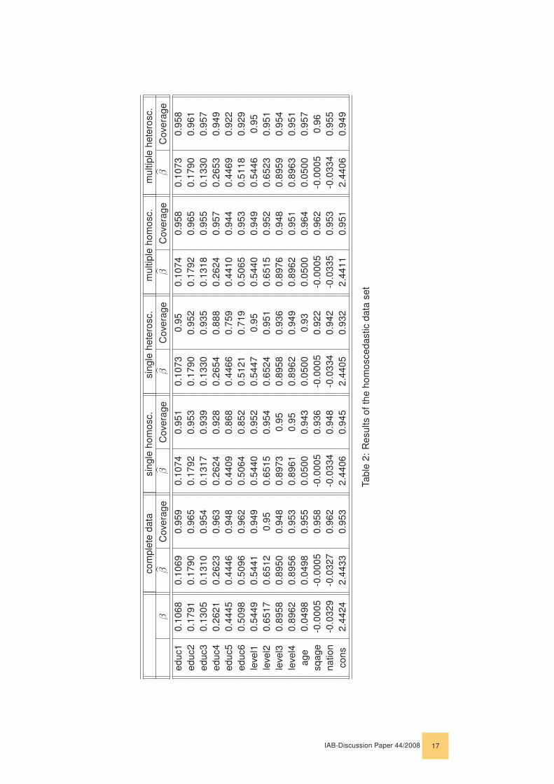
4 Results

This chapter contains tables showing the results of the simulation study comparing the

four different approaches. The first column presents the true parameters β of the original

complete population. The following columns show the estimates β̂ (here the average of the

1000 iterations) of the regression using the 10 percent complete random samples and the

regressions using the data sets imputed by the different approaches. The tables show as

well the fraction of iterations where the 95 percent confidence interval based on β̂ contains

β (coverage).

4.1 Homoscedastic data set

Table 2 shows the results of the simulation based on the homoscedastic data set A. As ex-

pected, the simulation study shows the necessity of a multiple imputation approach, since

the coverage of the two multiple imputation approaches is higher compared to the single

imputations throughout almost all variables. Using a homoscedastic data set, the results

do not show serious differences between the homoscedastic and the heteroscedastic mul-

tiple imputation. We receive a coverage for both of these approaches around 95 percent


(between 0.922 and 0.965) - similar to the coverage received by the estimations using the

complete random samples (between 0.948 and 0.965) - which refers to a good imputation

quality. The coverage of the single imputations is for most of the variables lower than 0.95

- which indicates underestimated variances. Consequently, it can be concluded, that in

case of a homoscedastic structure of the residuals, it is advisable to use a multiple impu-

tation approach. However it does not matter if the algorithm considering heteroscedasticity

is chosen in the homoscedastic case, since it just represents a generalization of the ho-

moscedastic approach and therefore works well in case of homoscedasticity.

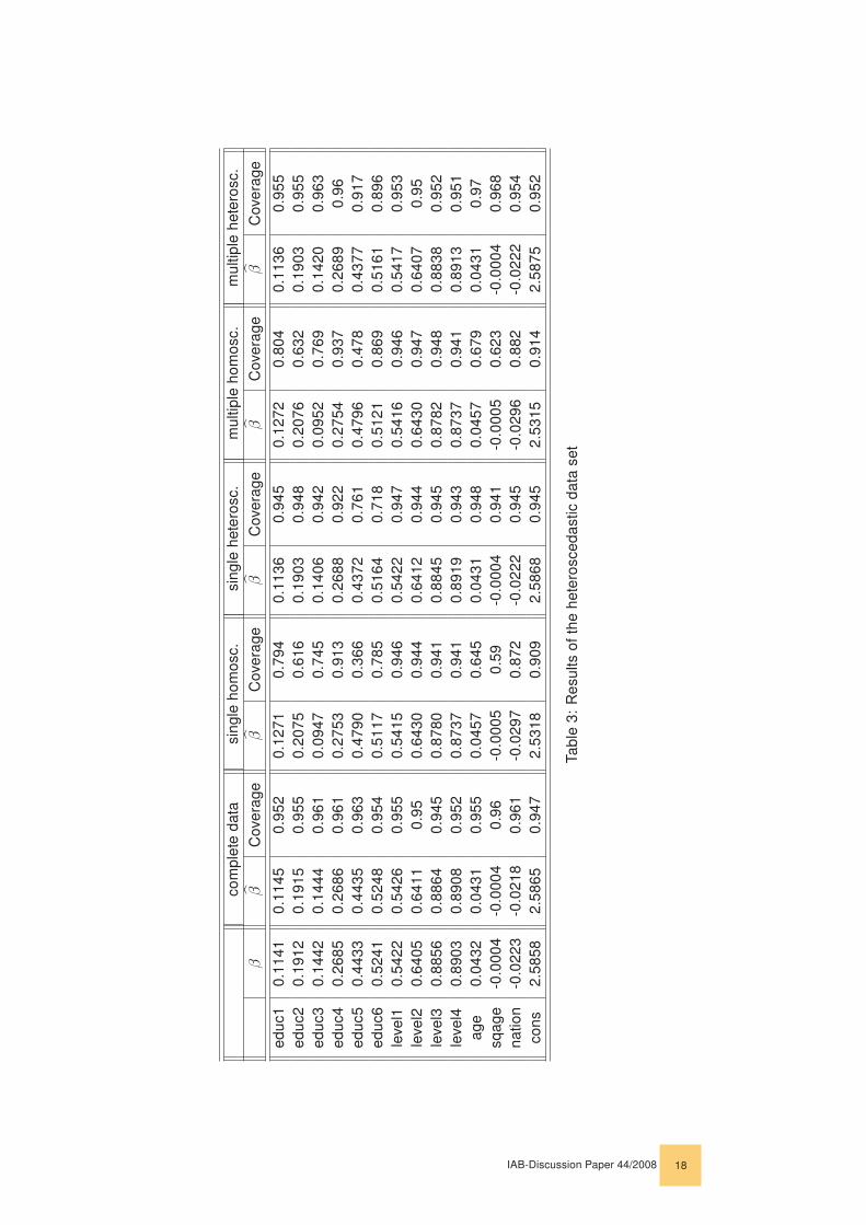
4.2 Heteroscedastic data set

The results based on the heteroscedastic data set B (Table 3) show a different situation.

The results recommend as well the use of a multiple imputation approach, since the cov-

erage of the single imputation approaches is again lower than 0.95 for all variables. But

concerning the heteroscedastic structure of the residuals, it reveals the necessity of an

approach considering heteroscedasticity. The homoscedastic approaches lead in several

cases to a considerably lower coverage than the procedures that consider heteroscedas-

ticity. The coverage of the heteroscedastic multiple imputation approach amounts again

to around 95 percent and is similar to the coverage based on the complete samples (the

coverage ranges between 0.917 and 0.97, except the dummy for the highest education

level where the coverage is 0.896). Thus we see that in this case, the coverage of the mul-

tiple imputation approach assuming homoscedasticity is lower (between 0.478 and 0.948,

for some variables even lower than the coverage received by the heteroscedastic single

imputation approach, where the coverage ranges between 0.718 and 0.948). Therefore

the results suggest the use of an approach considering heteroscedasticity to impute the

missing wage information in case of either an homoscedastic or heteroscedastic structure

of the residuals .

5 Conclusion

There is a wide range of ways to deal with censored wage data. We propose to use

imputation approaches to estimate the missing wage information. Nevertheless, there are

also different possibilities to impute the wages in the IAB employment sample, for example

single and multiple imputation approaches. Another important question is whether the

wages should be imputed considering heteroscedasticity or not.

In this paper we propose a new approach to multiply impute the missing wage information

above the limit of the social security in the IAB employment sample. We have assumed

that the variance of income is smaller in lower wage categories than in higher categories.

Thus we have suggested and developed a multiple imputation approach considering het-

eroscedasticity to impute the missing wage information. The basic element of this approach

is to impute the missing wages by draws of a random variable from a truncated distribution,

based on Markov chain Monte Carlo techniques. The main innovation of the suggested


com

plet

eda

tasi

ngle

hom

osc.

sing

lehe

tero

sc.

mul

tiple

hom

osc.

mul

tiple

hete

rosc

.

ββ̂

Co v

erag

eβ̂

Co v

erag

eβ̂

Co v

erag

eβ̂

Co v

erag

eβ̂

Co v

erag

e

educ

10.

1068

0.10

690.

959

0.10

740.

951

0.10

730.

950.

1074

0.95

80.

1073

0.95

8ed

uc2

0.17

910.

1790

0.96

50.

1792

0.95

30.

1790

0.95

20.

1792

0.96

50.

1790

0.96

1ed

uc3

0.13

050.

1310

0.95

40.

1317

0.93

90.

1330

0.93

50.

1318

0.95

50.

1330

0.95

7ed

uc4

0.26

210.

2623

0.96

30.

2624

0.92

80.

2654

0.88

80.

2624

0.95

70.

2653

0.94

9ed

uc5

0.44

450.

4446

0.94

80.

4409

0.86

80.

4466

0.75

90.

4410

0.94

40.

4469

0.92

2ed

uc6

0.50

980.

5096

0.96

20.

5064

0.85

20.

5121

0.71

90.

5065

0.95

30.

5118

0.92

9le

vel1

0.54

490.

5441

0.94

90.

5440

0.95

20.

5447

0.95

0.54

400.

949

0.54

460.

95le

vel2

0.65

170.

6512

0.95

0.65

150.

954

0.65

240.

951

0.65

150.

952

0.65

230.

951

leve

l30.

8958

0.89

500.

948

0.89

730.

950.

8958

0.93

60.

8976

0.94

80.

8959

0.95

4le

vel4

0.89

620.

8956

0.95

30.

8961

0.95

0.89

620.

949

0.89

620.

951

0.89

630.

951

age

0.04

980.

0498

0.95

50.

0500

0.94

30.

0500

0.93

0.05

000.

964

0.05

000.

957

sqag

e-0

.000

5-0

.000

50.

958

-0.0

005

0.93

6-0

.000

50.

922

-0.0

005

0.96

2-0

.000

50.

96na

tion

-0.0

329

-0.0

327

0.96

2-0

.033

40.

948

-0.0

334

0.94

2-0

.033

50.

953

-0.0

334

0.95

5co

ns2.

4424

2.44

330.

953

2.44

060.

945

2.44

050.

932

2.44

110.

951

2.44

060.

949

T abl

e2:

Res

ults

ofth

eho

mos

ceda

stic

data

set


com

plet

eda

tasi

ngle

hom

osc.

sing

lehe

tero

sc.

mul

tiple

hom

osc.

mul

tiple

hete

rosc

.

ββ̂

Co v

erag

eβ̂

Co v

erag

eβ̂

Co v

erag

eβ̂

Co v

erag

eβ̂

Co v

erag

e

educ

10.

1141

0.11

450.

952

0.12

710.

794

0.11

360.

945

0.12

720.

804

0.11

360.

955

educ

20.

1912

0.19

150.

955

0.20

750.

616

0.19

030.

948

0.20

760.

632

0.19

030.

955

educ

30.

1442

0.14

440.

961

0.09

470.

745

0.14

060.

942

0.09

520.

769

0.14

200.

963

educ

40.

2685

0.26

860.

961

0.27

530.

913

0.26

880.

922

0.27

540.

937

0.26

890.

96ed

uc5

0.44

330.

4435

0.96

30.

4790

0.36

60.

4372

0.76

10.

4796

0.47

80.

4377

0.91

7ed

uc6

0.52

410.

5248

0.95

40.

5117

0.78

50.

5164

0.71

80.

5121

0.86

90.

5161

0.89

6le

vel1

0.54

220.

5426

0.95

50.

5415

0.94

60.

5422

0.94

70.

5416

0.94

60.

5417

0.95

3le

vel2

0.64

050.

6411

0.95

0.64

300.

944

0.64

120.

944

0.64

300.

947

0.64

070.

95le

vel3

0.88

560.

8864

0.94

50.

8780

0.94

10.

8845

0.94

50.

8782

0.94

80.

8838

0.95

2le

vel4

0.89

030.

8908

0.95

20.

8737

0.94

10.

8919

0.94

30.

8737

0.94

10.

8913

0.95

1ag

e0.

0432

0.04

310.

955

0.04

570.

645

0.04

310.

948

0.04

570.

679

0.04

310.

97sq

age

-0.0

004

-0.0

004

0.96

-0.0

005

0.59

-0.0

004

0.94

1-0

.000

50.

623

-0.0

004

0.96

8na

tion

-0.0

223

-0.0

218

0.96

1-0

.029

70.

872

-0.0

222

0.94

5-0

.029

60.

882

-0.0

222

0.95

4co

ns2.

5858

2.58

650.

947

2.53

180.

909

2.58

680.

945

2.53

150.

914

2.58

750.

952

T abl

e3:

Res

ults

ofth

ehe

tero

sced

astic

data

set


approach is to perform additional draws for the parameter γ describing the heteroscedas-

ticity in order to be able to allow individual variances for every individual. To confirm the

necessity and validity of this new method we have used a simulation study to compare the

different approaches. The results of the simulation study can be summarized as follows:

The missing wage information should be imputed multiply, because single imputations may

lead to biased variance estimations. Furthermore, the imputation should be done consid-

ering heteroscedasticity. As the assumption of homoscedasticity is highly questionable

with wage data, the simulation study shows it is preferable to use the new approach con-

sidering heteroscedasticity, as this approach is more general: In case of homoscedastic

residuals the same quality of imputation results can be expected compared to the Gart-

ner and Rässler (2005) approach. But if heteroscedasticity is existent the simulation study

confirms the necessity of our new approach.


6 References

Bender, S., Haas, A. and Klose, C. (2000). IAB Employment Subsample 1975-1995. Op-

portunities for Analysis Provided by Anonymised Subsample. IZA Discussion Paper

no. 117, Bonn.

Gartner, H. (2005). The imputation of wages above the contribution limit with the German

IAB employment sample. FDZ Methodenreport 2/2005, Nürnberg.

Gartner, H. and Rässler, S. (2005). Analyzing the changing gender wage gap based on

multiply imputed right censored wages. IAB Discussion Paper 05/2005, Nürnberg.

Greene, W.H. (2008). Econometric Analysis, 6th ed., Prentice Hall.

Jensen, U., Gartner, H. and Rässler, S. (2006). Measuring overeducation with earnings

frontiers and multiply imputed censored income data. IAB Discussion Paper 11/2006,

Nürnberg.

Little, R.J.A and Rubin D.R. (1987). Statistical Analysis with Missing Data. Wiley, New

York.

Little, R.J.A and Rubin D.R. (2002). Statistical Analysis with Missing Data, 2nd ed. Wiley,

Hoboken.

Rässler, S. (2006). Der Einsatz von Missing Data Techniken in der Arbeitsmarktforschung

des IAB. Allgemeines Statistisches Archiv, 90, 527-552.

Rässler, S., Rubin D.B., Schenker, N. (2007). Incomplete data: Diagnosis, imputation and

estimation. In: de Leeuw, E., Hox, J., Dillman, D. (Eds.), The international Handbook

of Survey Research Methodology. Sage, Thousands Oaks.

Rubin, D.B. (1978). Multiple imputation in sample surveys - a phenomenological Bayesian

approach to nonresponse. Proceedings of the Survey Methods Sections of the Amer-

ican Statistical Association, 20-40.

Rubin, D.B. (1987). Multiple Imputation for Nonresponse in Surveys. Wiley, New York.

Rubin, D.B. (2004a). Multiple Imputation for Nonresponse in Surveys, 2nd ed. Wiley, New

York.

Rubin, D.B. (2004b). The design of a general and flexible system for handling nonre-

sponse in sample surveys. The American Statistician, 58, 298-302.

Schafer, J.L. (1997). Analysis of Incomplete Multivariate Data. Chapman & Hall, New

York.


Recently published

No. Author(s) Title Date 29/2008 Stephan, G.

Pahnke, A. A pairwise comparison of the effectiveness of selected active labour market programmes in Germany

7/08

30/2008 Moritz, M. Spatial effects of open borders on the Czech labour market

7/08

31/2008 Fuchs, J. Söhnlein, D. Weber, B.

Demographic effects on the German labour supply: A decomposition analysis

8/08

32/2008 Brixy, U. Sternberg, R.. Stüber, H.

From Potential to Real Entrepreneurship 8/08

33/2008 Garloff, A. Minimum Wages, Wage Dispersion and Unem-ployment

8/08

34/2008 Bruckmeier, K. Graf, T. Rudolph, H.

Working poor: Arm oder bedürftig? 8/08

35/2008 Matthes, B. Burkert, C. Biersack, W.

Berufssegmente: Eine empirisch fundierte Neu-abgrenzung vergleichbarer beruflicher Einheiten

8/08

36/2008 Horbach, J. Blien, U. von Hauff, M.

Structural Change and Performance of the German Environmental Sector

9/08

37/2008 Kirchner, St. Oppen, M. Bellmann, L.

Zur gesellschaftlichen Einbettung von Organisa-tionswandel: Einführungsdynamik dezentraler Organisationsstrukturen

9/08

38/2008 Kruppe, Th. Rudloff, K.

Wirksamkeit beruflicher Weiterbildungsmaßnah-men: Eine mirkoökonometrische Evaluation der Ergänzung durch das ESF-BA-Programm in der Zeit von 2000 bis 2002 auf Basis von Prozessdaten der Bundesagentur für Arbeit

9/08

39/2008 Brixy, U. Welche Betriebe werden verlagert: Beweggründe und Bedeutung von Betriebsverlagerungen

10/08

40/2008 Oberschachtsiek, D.

Founders’ Experience and Self-Employment Duration : The Importance of Being a ’Jack-of-all-Trades’. An Analysis Based on Competing Risks

10/08

41/2008 Kropp, P. Schwengler, B.

Abgrenzung von Wirtschaftsräumen auf der Grundlage von Pendlerverflechtungen : Ein Methodenvergleich

10/08

42/2008 Krug, G. Popp, S.

Soziale Herkunft und Bildungsziele von Jugend-lichen im Armutsbereich

12/08

43/2008 Hofmann, B. Work Incentives? Ex-Post Effects of Unemploy-ment Insurance Sanctions : Evidence from West Germany

12/08

As per: 17.12.2008

For a full list, consult the IAB website http://www.iab.de/de/publikationen/discussionpaper.aspx

http://www.iab.de/de/389/section.aspx/Publikation/k080729a05�

http://www.iab.de/de/389/section.aspx/Publikation/k080731n02�














http://www.iab.de/de/publikationen/discussionpaper.aspx�

Imprint

IAB-Discussion Paper 44/2008

Editorial addressInstitute for Employment Research of the Federal Employment AgencyRegensburger Str. 104D-90478 Nuremberg

Editorial staffRegina Stoll, Jutta Palm-Nowak

Technical completionJutta Sebald

All rights reservedReproduction and distribution in any form, also in parts, requires the permission of IAB Nuremberg

Websitehttp://www.iab.de

Download of this Discussion Paperhttp://doku.iab.de/discussionpapers/2008/dp4408.pdf

For further inquiries contact the author:

Thomas BüttnerPhone +49.911.179 3165E-mail [email protected]

Documents

IAB Discussion Paper 44/2008doku.iab.de/discussionpapers/2008/dp4408.pdf · We treat this problem as a missing data problem and derive new multiple imputation approaches to impute