Remote Data Access and Analysis using SciDB

by

ARCHIVESMASSACHU T

.i § ......

Alan M. Anderson

Submitted to the Department of Electrical Engineering

and Computer Science

in Partial Fulfillment of the Requirements for the Degree of

Master of Engineering in Electrical Engineering and Computer Science

at the Massachusetts Institute of Technology

February 2012

Copyright 2012 Alan M. Anderson. All rights reserved.

The author hereby grants to M.I.T. permission to reproduce andto distribute publicly paper and electronic copies of this thesis document in whole and in part in

any medium now known or hereafter created.

Author:

Certified by:

Certified by:

Accepted by:

Department of Electrical Engineering and Computer ScienceFebruary 1, 2012

rA4

Lewis dirod, Research Scientist, Thesis Supervisorr oq~ 1,2012

IamMaddenAssociate Professor, Thesis Co-Supervisor1, 2012

Prof.'eDnnis M. Freeman, Chairman, Masters of EngineeringThesis Committee

2

Remote Data Access and Analysis using SciDBby

Alan M. AndersonSubmitted to the

Department of Electrical Engineering and Computer Science

February 1, 2012

In Partial Fulfillment of the Requirements for the Degree ofMaster of Engineering in Electrical Engineering and Computer Science

ABSTRACT

SciDB is an innovative data analysis system that provides fast querying and manipulation of large

amounts of time-series, scientific data. This thesis describes the design of a framework that provides a

user interface to SciDB that facilitates interactive processing of large datasets and supports long-running

batch jobs on a remote server or cluster. Using this interface, python user scripts access SciDB data,

process it, and write new result arrays. The framework addresses problems such as garbage collection,

data access permissions and maintenance of provenance. We present a case study in which we apply

this framework to data from the WaterWiSe project, and analyze the runtime performance of the

system.

3

Acknowledgments

I would like to start out by thanking my thesis advisor Lewis Girod who has provided me with two

separate research opportunities and has mentored me throughout the learning process. He assisted me

in finding funding and giving me the chance to spend part of a semester in Singapore. His expertise and

insight helped motivate and drive the vision of the research as he provided me with the spring board to

completion. Furthermore, he was patient with me from the first revision to the last.

I would like to thank Sam Madden who has been the head PI on three of my research projects which

culminated in my receiving a Masters of Engineering.

I would like to thank my Academic Advisor Dorothy Curtis, for spending hours helping me solve various

scheduling, funding, and research problems. She has volunteered countless hours and has offered a

tremendous amount of experience and guidance.

I would like to thank my mother, Judy Wendt, for being a motivating force when the words weren't

coming and the research was stalling. Furthermore, she offered herself as a sounding board and a proof

reader.

I would like to thank my one year old son Luke, who relieved so much stress and worry with his

continuous smile and endless energy. He gave me someone to chase around the apartment during

those much needed breaks.

Last but definitely not least, I would like to thank my wife Heather Anderson, who was always there

when I needed her and always out of the way when I needed get work done. She has supported me and

been a pillar of strength for the past four years and she deserves a degree as much as I do.

4

5

Table of Contents

ABSTRACT ................................................................................................................................... 3

Ta ble of Contents .................................................................................................................................... 6

Chapter 1 Introduction .......................................................................................................................... 13

1.1 Project Background....................................................................................................................13

1.1.1 Im proving Data Representation and Access..................................................................... 15

1.1.2 SciDB..................................................................................................................................16

Chapter 2 Requirements........................................................................................................................18

2.1 DataSet .................................................................................................................................. 18

2.2 Rem ote Session......................................................................................................................19

Chapter 3 Design ................................................................................................................................... 21

3.1 SciDB......................................................................................................................................21

3.1.1 Array Layout..........................................................................................................................21

3.1.2 Data Loader....................................................................................................................21

3.1.3 The Python Connector................................................................................................ 22

3 .2 Se rv e r .................................................................................................................................... 2 7

3.2.1 Connection Handler (W W Server)................................................................................. 27

3.2.2 Request Handler (ServerThread)................................................................................. 28

3.2.3 Script Evaluator .............................................................................................................. 28

3.2.4 Installation and Configuration .................................................................................... 30

6

3 .3 C lie n t ................................................................................................................................. 3 3

3.4 Protocol ............................................................................................................................. 34

Chapter 4 Case Study - W aterW iSe ..................................................................................................... 36

4.1 Pre-existing File Hierarchy ................................................................................................... 36

4.2 Array Layout........................................................................................................................... 38

4.3 W aterW iSe Data Loader..................................................................................................... 41

DataProducer. ............................................................................................................................... 41

4.4 Configuration ......................................................................................................................... 44

4.5 Sam ple Data Processing Algorithm ..................................................................................... 45

Chapter 5 Analysis ................................................................................................................................. 48

5.1 Experiment Set Up ................................................................................................................. 48

5.2 Experiment Execution ............................................................................................................ 49

5.3 Experim ental Results ................................................................................................................... 50

5.3.1 Results of querying one quarter of a chunk................................................................. 51

5.3.2 Performance for long arrays. ...................................................................................... 53

5.3.3 SciDBiterator..................................................................................................................54

5.4 Discussion............................................................................................................................55

Chapter 6 Future W ork.......................................................................................................................... 57

6.1 Security and Authentication ................................................................................................... 57

6.2 Garbage Collection....................................................................................................................... 58

6.3 Parallelization ........................................................................................................................ 58

7

6 .4 Lo gg ing .................................................................................................................................. 58

6.5 Graphical User Interface..................................................................................................... 59

6.6 Data import to SciDB .............................................................................................................. 59

Chapter 7 Relate d W ork ........................................................................................................................ 60

7 .1 N u m Py ................................................................................................................................... 60

7 .2 SciPy ...................................................................................................................................... 6 0

7.4 M AT AB.................................................................................................................................60

7 .5 Ipyth o n .................................................................................................................................. 6 1

Chapter 8 Conclusion.............................................................................................................................62

B ib liog ra p h y .......................................................................................................................................... 6 3

8

List of FiguresFigure 1.1-1: Model of the sensors and nodes - The sensors are placed in the pipes and connected to

nodes on the surface. The nodes transmit the data through a satellite to the server. [2]..........15

Figure 3-1: Sample script demonstrating the use of a SciDB DataSet................................................. 26

Figure 4-1: The SciDB array has Node ID on the horizontal axis and Time on the vertical axis. At each

coordinate in the grid is four values, one for each of the sensor types. If the sensor didn't

produce a sam ple in that index, the value is null. ................................................................. 39

Figure 4-2: Data Producer which delivers all the files to the Data Consumer in the proper order...........42

Figure 4-3: This shows how the Data Consumer works. There is a Data Producer for each sensor that

outputs the value and index of the next piece of data. The lines above represent Data Samples

by each of the Sensors. Hydrophone produces 1 sample every index. PH and ORP produce 1

sample every 60,000 indices. Pressure produces 1 sample every 250 indices (not to scale). The

Data Consumer essentially has a sliding bar that moves forward in time 1 index at a time. It then

inputs the values from each DataProducer that has data for that index. ............................... 44

Figure 4-4: M udasser Iqbal's MaxDrop algorithm pipeline. ............................................................... 46

Figure 5-1: PRESSURE1920000, with reads of /4 the size of a chunk on node 17. The index is adjusted

where index 213926400000 -> 0 This data is from 22 May 2011.......................................... 51

Figure 5-2: Pressure query results with chunk size of 7680000. ........................................................ 52

Figure 5-3: Average request time vs. length of dataset. Generated using PRESSURE data..................53

Figure 5-4: The raw values showing longer queries have greater variance in performance.................54

Figure 5-5: Performance of iterating over every element of an array. Amount of data vs. Latency shows

the length of the data is linearly proportional to the latency of iteration...................................55

9

10

List of Tables

Table 3-1: This table shows the Database Schema involved with the Script execution including each Job,

the Job Queue and the progress of each job in the Flags Table. There is a one to one

relationship between the Jobs and Job Queue tables on the joblD field. There is a one to many

relationship between the Jobs to Flags tables on the JoblD field. ........................................ 30

Table 5-1: The tables I used for the analysis looked like this table. The indicies went from 0 to

172800000, (There are 172800000 indices per day). The nodeid included 17,19 and 20. There

was one attribute at each location, whose attribute was one of PH,ORP,PRESSURE, and

HYDROPHONE. There were six copies of each table, each with different chunk sizes...........48

Table 5-2: A list of the tables created for the analysis ....................................................................... 49

11

12

Chapter 1 Introduction

This thesis lays out the design of a software system which provides access to the raw, high resolution

data collected by the WaterWiSe project. WaterWiSe is a prototype wireless sensor network that

monitors Singapore's water distribution network in real time. WaterWiSe is a project being developed

by the Center for Environmental Sensing and Modeling (CENSAM), in collaboration with Nanjing

Technical University (NTU), National University of Singapore (NUS), and the Singapore Public Utilities

Board (PUB). CENSAM is a research department of the Singapore-MIT Alliance for Research and

Technology (SMART). In the WaterWiSe system, dozens of pressure sensors are distributed throughout

Singapore's urban water distributions network, providing data on the order of 1000 samples per second.

The project currently has several terabytes of data dating back to the start of the project in 2009. Prior

to our work, managing, analyzing, and summarizing this data was extremely cumbersome for the

researchers and involved in the project who needed access the high resolution, raw data. In this work

we outline the capabilities and the design of a system which simplifies this process.

1.1 Project Background

Started in January 2008, with funding and support from the MIT-Singapore Alliance, CENSAM works on

research focusing on environmental sensibility and modeling.

In the WaterWiSe project, the goal is to develop a "wireless sensor network to support continuous

monitoring of water distribution systems." [1] This system would provide a low-cost online method to

capture and analyze parameters of interest to those who design and maintain large urban water

distribution systems, from many points across a complex distribution network.

13

Such a system has numerous applications. By collecting this data, researchers can develop more

accurate hydraulic models, and in this way better understand the distribution system without relying on

assumptions and models that may be inaccurate. By making the data accessible on-line, measured

hydraulic parameters can be fed back into a live model in real time, resulting in a model with much

greater predictive power.

Another application is real-time monitoring of water quality. By combining data from water quality

sensors with a more accurate hydraulic system model, the impact of water quality events can be

predicted and it becomes possible to quickly protect an urban water system from contaminants

introduced into the network, by shutting the appropriate valves.

A third application of interest is burst and leak detection. Pipe bursts typically generate a pressure

transient that propagates through the network away from the burst location. By detecting these

transients at multiple points in the system, and by understanding the hydraulic parameters of the

system, it is possible to detect and localize pipe burst events. Prior to this project, this had been

demonstrated in laboratory conditions, and WaterWiSE was the first positive result from a real fielded

system. Leak detection can also be facilitated by this system, through analysis of the acoustic signature

of the system from many locations.

For the most part, the first application is finished as the beta version of the hardware is in use and

collecting data. However, the second two applications are still under development. For this thesis, I

helped complete segments of each of these applications. I created a portal that provides a

programmatic interface to the data across a local or wide area network. This helps enable real-time

monitoring of the water signals and allow for increased analysis for the raw-data.

As shown in Figure 1, the sensors are tapped into the water pipe at various locations to test pressure,

oxidation reduction potential, and pH level. The sensors are then wired to a small station or node on

14

the service, which consists of a small processor, flash storage, and a wireless transmitter. Eight different

nodes in place have been transmitting data for over three years, with a total of 25 nodes currently on-

line.

Enclosure box(sensor node processing

unit and batteries)

Solar panel,3G & GPS

antenna

Manhole (tappingpoint is inside)

Figure 1.1-1: Model of the sensors and nodes - The sensors are placed in the pipes and connectedto nodes on the surface. The nodes transmit the data through a satellite to the server. [2]

1.1.1 Improving Data Representation and Access

The existing system stores all of the data in a large archive of flat files, ordered by date and time.

Pressure and Hydrophone data is stored as binary files, while water quality data is stored as ASCII files.

In order to access the raw data files permission would need to be given by the network administrator to

open a port for file transfers. Once the port was open, the user could download the desired data files.

Before analyzing the data, the raw data would need to be calibrated to convert the raw values into

engineering units. This calibration data is specific to each node and changes over time as sensors are

periodically swapped out or recalibrated.

While this arrangement is acceptable for an off-line data archive, it is unnecessarily cumbersome to

extract data from the archive efficiently for the purposes of analysis or processing. In addition to the

complexity of extracting the data, it is often important to process very large volumes of data. For

15

example, a researcher who developed a modified burst detection algorithm might want to test this

algorithm over several years of data from the system. Typical analysis software packages such as

MATLAB or Octave are not designed to directly process extremely large time-series. Instead,

considerable effort must be put into writing code to get the data into and out of these packages.

1.1.2 SciDB

The primary focus of our work was to improve the ability of researchers to access, process, and analyze

this data. For this work we chose to use SciDB as the basis for our data management system. SciDB is a

Database Management System (DBMS) used to index large amounts of scientific data for fast analysis

and calculation. SciDB is not a traditional DBMS but rather a DMAS or Data Management and Analytics

Software Solution, and where other DBMS implementations are designed for relational queries on

collections of tuples with no a priori ordering, SciDB is specifically designed to support time series data.

The primary drawback of SciDB from the outset was that it was a moving target, with frequent releases

and API changes. While it was difficult to deal with the changing API and the development of new

features, overall SciDB helped to progress the work significantly.

SciDB is not a relational database, but rather an array-oriented database. Instead of records, SciDB has

arrays. Instead of fields, an array has attributes and indices. The underlying data representation of a

SciDB database stores array data in fixed-size chunks. Chunks are the building blocks of arrays, and as

such each chunk has the same order as the array to which it pertains (has the same number of

dimensions).

A chunk is the physical unit of 1/0, processing and inter-node communication. When an array with n

attributes is saved to disk, SciDB's storage manager separates the array into n arrays each with one

attribute. This is done behind the scenes and is not exposed to the user. Then it separates all of the

data into equally sized, potentially overlapping chunks. All data in a chunk is stored in contiguous

16

addresses on disk to take advantage of locality. Whenever part of the data in a chunk is accessed, the

entire chunk is loaded into memory.

Chunks are important for a variety of reasons and the chunk sizes are fully configurable. The chunk size

is the smallest amount of data that is put in memory when part of the data is queried. As such, if the

chunks are too big, then each query will transfer more data onto memory than is needed. When chunks

are too small, the benefit of storing the data in columns is lost. The chunk size is also the smallest

amount of data that is sent across the network when being used on a cloud. If the chunk size is too

small, then the overhead of the packets is larger in proportion to the amount of data that is sent. If the

chunk size is too big, then packet failures result in a lot of lost data and retransmission. Additionally,

when a chunk is too large extraneous data may be loaded resulting in addition latency. It has previously

been researched and found that the optimal chunk size is around 4-8 MB.

SciDB is also being developed with the concept of parallel computing on a cloud. It is developed so that

SciDB can be deployed on multiple machines, with one designated as the master and the rest as slaves,

and configured for data sharing and manipulation.

17

Chapter 2 Requirements

This work was inspired by three key requirements of the WaterWiSe project. First, we needed a

convenient way to access the large amounts of data generated by the system. Second, we needed to

perform complex, time intensive calculations on these large datasets. Third, we needed a way to save

intermediate data and large resultant datasets. All of these functions should be accessible remotely in

order to support utility computational services.

2.1 DataSet

The WaterWiSe system archives data in a sequence of flat files. Although simple, accessing and

processing the data was quite straight forward, the API has need to support both retrieving data and

saving new and calculated data. The data in a dataset must be able to hold the raw data from the

sensors as well as any data that is the result of a calculation on a raw dataset. For example, if a user

performs a Fast Fourier Transform (or any other transformation) on 6 months of data, it should be

possible to save the result into the database as a new array. While the data would reside on the server,

it could be accessed or downloaded from the client, or viewed on a web page.

Provenance. Provenance is the ability to describe the source and derivation of data. Since there is an

ever increasing amount of raw data and calculated arrays, the arrays will need to be garbage collected in

some way. However, if an array is garbage collected and a user needs to access that array, then the tool

needs to be able to regenerate the array. To accomplish this, the provenance of each dataset is

recorded in the form of a script that would regenerate it.

Mutable vs. Immutable Data. Provenance is much more complex if datasets are allowed to be mutable.

If they are mutable, then every manipulation must be recorded so that the array could be recreated in

the event of garbage collection. This concern fits well with the design of SciDB, which defines all arrays

18

as immutable. An immutable data model also greatly simplifies parallel processing and caching schemes

that are critical for high performance applications. Thus, we have made a design choice to make all

arrays immutable.

2.2 Remote Session

With the data residing on a server, and with multiple users accessing the data from client machines,

users need to be able to log in to the server, access the data and perform calculations. To accomplish

this there must be some client-server protocol and authentication system in place.

Authentication. A user should need to be registered and should be able to log in in order to access the

data. This is not just a matter of security but rather a matter of functionality. Requiring authentication

allows the system to defer which data sets are visible to each user. Each array is owned and used by

certain user groups. If the user is not a member of any group associated with an array, then that array

would be invisible to that user. This prevents users from being overwhelmed with dozens of arrays that

are irrelevant to them.

Script Execution. Actions taken by the user to access and manipulate data on the server are

implemented by uploading a python script that is then executed on the server. The user script can use

any installed python library, including NumPy and should be able to use this tool to access and save

result arrays to SciDB. Since these scripts may be long-running operations, they must persist across

client sessions. The user should be able to check on the progress of any job they upload.

Interactive Sessions. A user can decide to engage in a remote session where they can enter python

commands. This would be run just like an interactive Python shell. The commands could be saved so

that the user would be able to suspend the session and log back in later to resume where they left off.

19

Security. For now the remote protocol needn't be secure, but a future extension could include using an

SSH encryption protocol, where the client and server exchange keys allowing messages from each party

to be encrypted.

20

Chapter 3 Design

The design is composed of three different modules. The first provides the interface glue between the

server and the SciDB API. This module handles the configuration of the SciDB arrays, the SciDB data

loader and the SciDB data retriever. The second module implements the server, including the client

protocol, job scheduling, authentication, and user and array metadata. The third module is the client

code including the protocol to communicate with the server and the user interface.

3.1 SciDB

This section describes the parts of SciDB that are particularly relevant to this system and gives an

overview of how SciDB interacts with the system, to provide fast access to the data for analysis.

3.1.1 Array Layout.An array is an n-dimensional SciDB object with a number of attributes stored at each location in the

coordinate system. Some values may be empty, others may be Null (SciDB treats these cases

differently), and the rest may have values. When an array is created in SciDB, all dimensions are named

with the maximum and minimum values defined; all attributes are defined specifying the data type. The

array is then defined in n dimensions with the possibility of m values at each location.

3.1.2 Data LoaderWith so much past data already stored on the server, and so much new data being generated every day,

I developed a module that is used to take past data from the raw files, calibrate it with the raw data,

then upload it to SciDB. This module is designed as a producer and consumer. The producer fetches the

raw data files in the proper order, while the consumer gets each file, one at a time, parses the data,

converts the datum to a calibrated value, then saves it to a file. Finally, it calls the SciDB load command.

The details of the data loader would primarily depend on the specifics of the application. We describe

our particular data loader implementation in more detail in Chapter 4.

21

3.1.3 The Python ConnectorWith the data in SciDB, there needs to be a way to access the data and to save data to SciDB. The

developers at SciDB have developed a python library to facilitate accessing the data and executing

queries on the database. To simplify the interface to SciDB I created a wrapper class that better suits

the needs of WaterWiSe.

The SciDB python package for retrieving the data has 2 important classes. The Chunkiterator is used to

iterate over all of the chunks in an array. The Constiterator is used to iterate over all of the data in a

chunk. For the purposes of WaterWiSe it isn't useful to deal with chunks, but rather to simply have

access to the time series data. There are also functions that get the metadata of arrays such as the

dimensions, the attributes, and a description of array.

SciDBiterator. To address this we developed the SciDBterator class, which hides the Constiterator and

the Chunkterator from the users and allows them to simply use one iterator. It takes as input a query,

the query language, and the attribute. The query is any query that SciDB can handle. SciDB has 2 query

languages that allow access and manipulation of the database, namely Array Query Language (AQL), and

Array Functional Language (AFL). Lastly, the attribute is a string passed in so the right attribute is

fetched. The result is a python iterator.

SciDBIteratorWrapper. Besides hiding the complicated iterator structure exposed by SciDB, it was also

important to hide the complicated query language as well. However, the SciDBIterator takes as an

argument a query string. While the SciDBIterator is flexible for expert users, most of WaterWise's users

will want to use the SciDBWrapper instead. The SciDBlteratorWrapper class takes an array name, a

starting index, an ending index, and an attribute. The SciDBiteratorWrapper will then generate and

execute the query. The result is an iterator with the data.

22

DataSet. Using the SciDBIterator users will frequently manipulate the data generating a resultant python

array. Users need a way to save that data to SciDB. The DataSet class takes an array, array name,

username, and array description as inputs. The array can be empty to start with. One of the

requirements for this project is provenance. As stated above, provenance is important because an array

may be garbage collected at any given point, even if it is still needed. When a garbage collected array is

needed the tool needs to have a way to recover that array. To accomplish this, a DataSet object must

have a record of how it was created. This problem is solved by requiring the user to designate either a

script that generates the array, or during a shell session, the user must define starting and ending points

in the session designating the lines of code that generate the new dataset. An example is listed below to

clarify how this works. The resultant array is the same as the input array at the local minimums and

maximums, and zero everywhere else. The first element is considered a max or a min depending on

what follows.

23

> # Create an array called MaxDrop with Username alan,> # Parameter 3 is the array description, parameter 4 by default is []> dataset=DataSet("MaxDrop", "alan", "run maxDrop on node 1")> dataset.execute(r"inputArr=SciDBIteratorWrapper('WaterWiSe',

214963200000, 214963255000,'PRESSURE'))> dataset.execute("result=[] ")> dataset.execute ("direction=None")> dataset.execute ("prev=None")> dataset.execute ("for> dataset . execute ("> dataset.execute ("> dataset.execute ("> dataset.execute ("> dataset . execute ("> dataset . execute ("> dataset . execute ("> dataset . execute ("> dataset . execute ("> dataset . execute ("> dataset.execute ("> dataset.execute ("> dataset . execute ("> dataset .execute ("> dataset . execute ("> dataset . execute ("> dataset .execute ("

i in inputArr:")if prev==None:")

pass")elif direction==None:"I)

if i<prev:")direction=-1" )

else:")direction=1" )

result .append (prev) ")elif i<prev and direction==1: ")

result .append (prev) ")direction= -1")

elif i>prev and direction==-1:")result .append (prev) ")direction=1 ")

else:")result.append(0) ")

prev=i ")dataset.execute ("result.append(0) ")dataset.setArray(result)print resultdataset.saveArray()

This code creates a dataset object, then uses that object to execute several lines. Each line gets saved to

a file whose name is a random universal unique id (UUID) with ".py" appended on the end. Each line is

also executed using python's exec command. After the user has executed each line, the user must

specify which variable to set as the array. It is noteworthy that the penultimate line that says "print

result" is not saved in the script used for provenance because it wasn't called using the dataset object.

Finally the user must call dataset.saveArrayo. So doing, adds the array to the MySQL arrays and uploads

the array to SciDB.

Provenance. I wish to clarify how provenance works with this tool. Suppose a user executes the code

above to create an array called MaxDrop. Now suppose the user generates a new array called

AbsoluteValueMaxDrop which simply returns the absolute value of every element in the MaxDrop array.

24

Now imagine other users generate many other arrays to the point where the 2 arrays generated above

get garbage collected. Finally, the initial user tries to access the AbsoluteValueMaxDrop array. In doing

so the tool would check if AbsoluteValueMaxDrop has been garbage collected. Seeing that it had it

would look up the path of the script that generated the AbsoluteValueMaxDrop in the MySQL database.

It would then execute that script. However, that script references the MaxDrop array. At that point the

tool would check and find out that the MaxDrop array has also been removed from SciDB. It would then

look up the script for the MaxDrop array and execute it. It could then return to the

AbsoluteValueMaxDrop script and finish executing it. At that point the user would have access to the

MaxDrop array as well as the AbsoluteValueMaxDrop array. This process is summarized in Figure 3-1.

Note that instead of typing all of the dataset.executeo commands in Figure 3-1we use Python's multiline

string option.

25

> # Create an array called MaxDrop with Username alan,> # Parameter 3 is the array description, parameter 4 by default is

[]> dataset=DataSet("MaxDrop", "alan", "run maxDrop on node 1")

> code= """inputArr=SciDBIteratorWrapper('WaterWise', 214963200000,214963255000,'PRESSURE'))result= []direction=Noneprev=Nonefor i in inputArr:

if prev==None:pass

elif direction==None:if i<prev:

direction=-1else:

direction=1result.append(prev)

elif i<prev and direction==l:result.append(prev)direction= -1

elif i>prev and direction==-1:result.append(prev)direction=1

else:result.append(0)

prev=iresult.append(0)

> dataset.execute(code)> dataset.setArray(result)> print result> dataset.saveArray()

Figure 3-1: Sample script demonstrating the use of a SciDB DataSet

Alternatively, the user could type the script into a file named MaxDrop.py (or any .py file), in which case

the code would look like the following:

> # Create an array called MaxDrop with Username alan,> # Parameter 3 is the array description, parameter 4 by default is

[]> dataset=DataSet("MaxDrop", "alan", "run FFT on node 1")> dataset.executeFile("./MaxDrop.py")> dataset.saveArray()

A user creates a DataSet object with the given parameters.

26

Then it saves the array to a file in the SciDB Sparse data format. Then it executes a CREATE ARRAY query

with the array name as <username>_<arrayname>_<number> where username and array name are the

parameters passed in and the number is added to the end in the event that the given user has an array

with the given name already. In which case the new array will be named uniquely and the existing array

will not be affected. The SaveArray command also adds a record into the MySQL database

The developers at SciDB are planning to develop new ways to load data, but for now the only solution is

to save the array to a temporary file, pipe, or fifo. In the future work section I mention that it would be

a beneficial exercise to implement a method to import a python array directly into SciDB without writing

to a file first.

3.2 Server

The server is made up of the Connection Handler and the Request Handler. The Connection Handler

waits for connections and refers clients to the RequestHandler when a connection is made. The

RequestHandler maintains the connection with the client responding appropriately to any request the

client might make. These requests could be uploading a script to the server, checking progress of an

uploaded script or even initiating a shell session. Below describes the parts that make up the server in

greater detail.

3.2.1 Connection Handler (WWServer)The connection handler is a class called WWServer. When this class's start() method is called it starts

listening on port 5001 (This can be changed with the configuration file) for connection requests. When a

client tries to connect the server spins a thread object called ServerThread and resumes listening for

new connections. The ServerThread class opens a socket to handle the client's requests. Once the

client breaks the connection the ServerThread object dies. At any one point in time the server can only

allow five people to be logged in at one time. This doesn't present a problem for WaterWiSe as the

27

team is currently small. If five people are logged in when a sixth user tries to connect the server queues

up that connection until one of the five users log off.

3.2.2 Request Handler (ServerThread)

The ServerThread class listens for requests from the user and returns a response just like a typical client

server protocol.

3.2.3 Script EvaluatorThe Script Evaluator allows a client to upload a script to the server which is then executed. While it is

being executed the user can check on the progress of the execution. Once it is completed the user can

request the standard output and the error output of the script.

Script. The type of script that can be executed is any python script that imports from the python

libraries already installed on the server. If a library is needed that isn't installed a user with sudo

privileges can install the library.

Upload and Initialization. When the file is uploaded to the server, the local name is a random UUID and

is saved in the ./JobProcessor/scripts/ directory. (Describe WWDBManager somewhere). Next the

MySQL database is updated by inserting a new row in the Jobs table with a description, owner, script

path, and status set. The description is given by the user, the owner is whoever is looked up by the tool

as the person currently logged in, the script path is the UUID generated when the script is uploaded, and

the status is "Downloading" initially. When it is done downloading the WWDBManager changes the

status to "Queued" and adds the job to the JobQueue table which just contains a timestamp and the

jobiD generated by the insert query into the Jobs table.

Script Execution. The server continuously has a service running behind the scenes. The script checks

the JobQueue table for a job. If there is no job it sits and waits for 30 seconds before trying again. If

there is a job in the queue it takes the joblD and gets the job information from the Jobs table. Then it

28

updates the status to "Running". It sets python's stdout to point to a file named as the UUID for the

filename with .out appended on the end. It sets python's stderr to point to a file named as the UUID

with .err appended on the end. Then it executes the python file. Once execution has finished the jobs

status is set to "Finished" and the job is deleted from the job queue. The server then continues checking

for any updates on the job queue every 30 seconds.

If the file raises an exception, the jobs attempt count is incremented in the Jobs table. The Job will then

start at the beginning and try to execute it again. If the attempt count reaches three the server removes

the job from the JobQueue and sets the status to "Cancelled with Errors" in the Jobs table.

Script Progress. As I mentioned earlier the user can check the status of any job by submitting the joblD

to the server. The server simply looks up the status in the Jobs table. The user can also check on the

progress of a running script. This is much more complicated. First the user needs to embed checkpoints

or flags in their code. Wherever they want a checkpoint they can insert the following command:

jobProcessUtil.setFlag(WWJobID,<NameOfTag>)

The jobProcessUtil library is already imported before the script is executed on the server, and the

WWJoblD variable is also defined using the Job ID from the Jobs table. NameOfTag can be any string the

user wants to use to identify the checkpoint. After embedding however many of those commands that

he\she wishes, the user needs to report how many check points there are when they submit the script.

When the jobProcessUtil.setFlag command is executed it inserts a record into the Flags table in the

MySQL database. If the user wishes to check on the progress of the script he/she sends the progress

request with the job id. The server then counts how many flags in the Flags table match the job ID and

looks up the TotalProgressCtrs field in the Jobs table which is the number of flags submitted by the user.

The server returns "<flagName> d/n" to the user where <flagName> is the name of the last flag inserted

29

by the script, d is the number of flags reached in the script, and n is the total number of flags as reported

by the user.

This solution has a few down sides, but provided the most accuracy. The first problem with this solution

is the user needs to be able to count or otherwise predict the number of flag counters that will be

executed. This requires additional work by the user, but it may also be impossible to know. For

example, if the user inserts a setFlag() command in a for loop with an unknown amount of iterations, the

user would have no way of knowing how many flags will be reached. To solve this problem, I could have

counted the number of lines in the file and report the progress based on the line number being

executed and the total number of lines. However this can be deceiving also if there is a very lengthy for

loop in a short script because the tool could report that most of the lines have been executed but the

execution will continue for a long time finishing the for loop. Line count doesn't indicate how much of

the script is executed. The method I chose also has the advantage of allowing the user to name the flags

so they can always know exactly what is going on with the script.

Int(11) NO PRI NULL auto-increment

m yoms ig . int(11) NO NULL

Int(11) NO PRI NULL auto-increment -- varchar(30) YES NULL

0 varchar(200) YES NULLvarchar(50) NO NULL NMltraLLvarchar(200) NO NULL int(11) No PRI NULL' auto incrementvarchar(200) YES NULL .. int(11) NO NOLLvarchar(20) NO NULL i - nt(11) NO 0

E int(11) NO1

Table 3-1: This table shows the Database Schema involved with the Script execution includingeach Job, the Job Queue and the progress of each job in the Flags Table. There is a one to onerelationship between the Jobs and Job Queue tables on the joblD field. There is a one to manyrelationship between the Jobs to Flags tables on the JobID field.

3.2.4 Installation and ConfigurationInstallation and Configuration is intentionally straight forward and simplistic, while still allowing all the

necessary functionality. This section outlines the installation procedures.

30

Hardware Requirements. The only hardware requirements for this system are those imposed by SciDB.

The requirements and installation instructions for SciDB can be found at:

http://www.scidb.org/

The system I was using had an Intel(R) Xeon(R) CPU E5430 processor with a clock speed of 2.66GHz and

four gigabytes of Memory.

Software Requirements. The only direct requirements include MySQL and SciDB. The system I used

had Ubuntu 9.10, MySQL version 5.1.37-lubuntu5.5, and SciDB Version 11.06 for 64 bit machines. These

are not requirements but rather systems that I know it works on.

SciDB has its own software requirements, but those will be taken care in the process of install SciDB, so I

do not mention them here.

Configuration. As I said earlier the configuration is extremely basic, and Chapter four I provide an

example configuration for a sample use case.

The configuration file is called config.py and only has eight values that can be adjusted. The first four

deal with the SciDB initialization and limits the admin wants to impose on the users.

> SENSORTYPES defines what sensors are operational in the system, represented as a list.

These are the attributes of the array.

> CHUNKSIZE defines how much data you want in each chunk. This specifies the number of

indices per chunk in the time dimension

> USERDEFINEDARRAYMAXCOUNT sets the maximum number of user defined arrays

before the tool starts garbage collecting arrays

o The default is arbitrarily set to 40, but can be set much higher if desired

31

> MAXDISKUTILIZATION sets the maximum amount of sciDB can use before the tool starts

garbage collecting arrays. Designated as a decimal between 0 and 1.

o Default - .85 representing 85 percent

The next two deal with important file locations.

> CODEROOT sets the root location for the src files to be installed.

o If left blank the current directory will be set as the default.

> DATAROOT tells tells the tool the root directory for the data.

o If left blank the current directory will be set as the default. The tool is useless if there is

no data so this must be set correctly.

The final two deal with the server configurations.

> SERVERPORT sets which port the server should listen on to establish connections. Note that

whatever is set as the port for the server must be set the same in the client's config.py file.

The client's configuration file is identical to the server's and just ignores the other values.

o Default - 5001

> LOGLEVEL sets the level of logging by the server. The least restrictive the level, the more

logs that will be logged. For example "DEBUG" will log all log statements, but "ERROR" will

only log ERROR and CRITICAL messages. Possible options, in order of least restrictive to

most restrictive, include: DEBUG, INFO, WARNING, ERROR, CRITICAL

o Default - Warning

Installation. Once the configuration file is saved and the software requirements are installed, the

installation is a one step process for the user. Ensure that the user has privileges to create tables in

MySQL and execute python setup.py install. The install file will create all of the MySQL tables needed

32

for the system. It will also issue the needed commands to create the data arrays in SciDB. The table

below shows the commands that are executed.

3.3 Client

The WWClient class exposes the API for clients wishing to connect to this system. The class has several

methods which are used to execute a session between the client and the server. It is important to note

that this protocol is not secure (see future work) and as such it may be a good idea to not expose the

server's ports publically but rather limit access to the Local area network.

A standard session between the client and server will consist of the user initializing the WWClient class,

calling the startSession() method, sending requests to the server, finally closing the connection. There

are several methods that can be called and I will list them now explaining what they do. Suppose c is a

WWClient object.

WWCliento - This is the constructor which simply generates the client object.

c.startSession() - This sends a message to the server and establishes a connection.

c.register() - This prompts the user for username and password, then requests that the server register

the user.

c.logino - This prompts the user for username and password, then requests that the server authenticate

the user.

c.uploadJob(filename) - This sends a file to the server to be executed. The return value is the job id.

c.jobsProgress(jobIlDs) - This requests the progress of the scripts uploaded by the user. joblDs is a list of

jobs whose progress the user wants. If the argument is omitted then all jobs' progress will be sent.,

otherwise, only the Jobs whose id is in the list are reported.

33

c.startSession(name) - This starts a shell session with the server. The name argument allows the user

to rejoin a previously started session if the user had previously started a session by that name.

Otherwise it starts a new session with the given name. The session behaves like an interactive python

session.

c.listScripts() - This returns a list of all the scripts that the current user has uploaded.

c.getOutput(scriptID) - This requests the output files for the given script id. The .out file is sent first,

then the .err file is sent.

c.listArrays() - This lists the SciDB arrays that are owned by any group the current user is a member of.

Many arrays are owned by the group "all" which means everyone can see them, and many arrays are

owned by an individual and are only visible for the owner.

c.getArray(arrayID) - This sends a json file containing the array data. The file is then read into a list.

c.logout() - This logs the user out of the session and breaks the connection.

3.4 ProtocolThis section describes exactly how the protocol works between the client and server. With sockets it is

necessary that the server and client receive exactly what they are expecting otherwise the server could

start waiting for a response while the client is waiting for a response and they get into a deadlock. This

is corrected by setting a time out, requiring the client to re-establish a connection with the server, and

with a very clear protocol.

Register:C: Register <Username> <HashedPW>S: False <Reason> | True

Login:C: Login <username> <hashedPW>

34

S: False <REASON> | True <Token>

Logout:

GetOutput:C: GETOUTPUT <ScriptID> <Token>S: FileSize I FALSE <Reason>S: <FILDATA> I FALSE <Reason>

ListArrays:C: LISTARRAYS <TOKEN>S: [arrl,arr2,.arrn] I FALSE <REASON>

ListScripts:C: LISTSCRIPTS <TOKEN>S: [jobidl,jobid2,.jobidn] I FALSE <REASON>

SendScript:C: RUNSCRIPT <FileSize> <Token>S: TRUE <JOBID> | FALSE <ERROR>C: <FILEDATA>S: TRUE I FALSE <ERROR>

ScriptProgress:C: SCRIPTSPROGRESS [[Namel,Name2,...NameN]] <TOKEN>S: <MESSAGE LENGTH> I FALSE <ERROR>S: <SCRIPT PROGRESS LIST>

StartShell:C: Shell [name] <token>S: TRUE | FALSE <ERROR>C: CommandS: LengthS: Output

35

Chapter 4 Case Study - WaterWiSe

As stated earlier, SciDB is in early stages of development and are actively seeking use cases for such a

data management and analysis software solution. WaterWiSe qualifies as one of the target users and

provides a very interesting use case. SciDB provides the engine that drives much of the functionality to

this project. This chapter is dedicated to a direct application to the system described in the previous

chapters.

4.1 Pre-existing File Hierarchy

This section explains the format of the raw data files as has existed in the past and continues being used.

The raw data files are stored in directories in the following format:

stn_<id>/data/<year>/<day>/<sensorType>/

where id is the node id, ranging from 10-36, year is the 4 digit year, day is the day number, ranging from

1-365 (366 on leap year), sensorType is the type of sensor. The types of sensors are BTRY,

HYRDROPHONE, ORP, PH, PHORP, PRESSURE.

Each file is also encoded with certain metadata in the filename. The format of the file changes with each

type of sensor. The PH and ORP files are encoded in the following format:

STN_<node id>_<yyyydddhhmmss>_<Sensor type>...<timezone>.raw

For example, a file named "STN_21_2011001010101_PHSGT.raw" contains PH data from station 21

starting in 2011 on day 001 at 01:01:01 am Singapore Time.

The Pressure and Hydrophone files are formatted the same as PH and ORP files up until the timezone

part of the path. After the sensor type the filename follows this format:

36

_<duration>_<sample size>_<microseconds>_<time zone>_<sample rate>.raw

Duration is in seconds, sample size is in bytes, and sample rate is samples per second. For example,

"STN_21_2011001010101_PRESSURE_30_2_000001_SGT_250.raw" represents pressure data on node

21 starting in 2011 on day 001 at 01:01:01.000001 AM Singapore Time lasting 30 seconds where each

sample is 2 bytes long at the rate of 250 samples per second. The file path for pressure and hydrophone

data is different because the times need to be more precise.

The BTRY files express the battery level. For the purposes of this thesis the BTRY data was ignored.

The HYDROPHONE data is sampled at 2000 samples per second. The data is stored as a two byte, little

endian signed integer. The raw data needs no calibrating since the hydrophone values are simply

recording the values.

The PRESSURE data is sampled at 250 samples per second. The data is stored as a two byte, little endian

signed integer. The actual data value is found by combining the sensor value with the calibration values

stored in a table on the server. The calibration equation where y is the calibrated value, x is the sensor

reading and m and b are the calibration values, is:

Y=mx+b

The ORP data is sampled every 30 seconds and is represented as a 4 byte float value stored in ASCII

format. ORP stands for oxidation reduction potential. The calibration equation simply contains an

offset value which is subtracted from the sensor reading to get the calibrated value:

y=x-offset

The PH value is sampled every 30 seconds and is represented as a 4 byte float value stored in ASCII

format. PH is the pH value of the water. The Calibration values are R=PHREF, p=PH_7 and m=SLOPE.

The Hydrophone calibration equation with y being the calibrated value and x being the sensor reading is:

37

y=7-(x-r-ph7)/(59.2*m)

The PHORP data is a representation of both PH and ORP data. As such there will either be PH and ORP

data or there will be PHORP data.

4.2 Array Layout.

The WaterWise data is stored in a two dimensional SciDB Array, time in one dimension and node id in

the other dimension. In the time dimension it starts on January 1st 2008 and has 2000 indices per

second. Each index is a 64 bit unsigned integer. In the node id dimension, the first index is 10 and

increments by one up to node 36, which is the last node in existence at the present. It is unbounded in

the positive direction which allows for adding more nodes.

Indices. The time index represents a uniform two kilohertz sample rate, but the start of each file is

recorded in microseconds. Therefore there may be a phase offset between the sample clock and the

actually data time. With 2000 indices per second and 1,000,000 microseconds per second I created a

mapping from microseconds to index. I wanted exactly 500 microseconds to map to every index, which

means the first 500 microseconds map to the first index. I created a function that takes a year, day,

hour, minute, second, and microsecond, and convert that time to an index. The function converts the

time data into a python datetime object and creates a datetime object representing January 1st 2008 at

12:00 am. Subtracting the two objects produces a timedelta object. The timedelta object tells how

many days, d, and how many seconds, s, and microseconds, m, separate the two datetime objects. The

index, I, is then calculated as:

i=2000(24*60*60*d+s)+[m/2000]

38

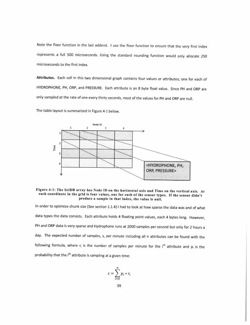
Note the floor function in the last addend. I use the floor function to ensure that the very first index

represents a full 500 microseconds. Using the standard rounding function would only allocate 250

microseconds to the first index.

Attributes. Each cell in this two dimensional graph contains four values or attributes; one for each of

HYDROPHONE, PH, ORP, and PRESSURE. Each attribute is an 8 byte float value. Since PH and ORP are

only sampled at the rate of one every thirty seconds, most of the values for PH and ORP are null.

The table layout is summarized in Figure 4-1 below.

Node ID1 2 3 4

1>

2

3

4

f

Figure 4-1: The SciDB array has Node ID on the horizontal axis and Time on the vertical axis. Ateach coordinate in the grid is four values, one for each of the sensor types. If the sensor didn't

produce a sample in that index, the value is null.

In order to optimize chunk size (See section 1.1.4) 1 had to look at how sparse the data was and of what

data types the data consists. Each attribute holds 4 floating point values, each 4 bytes long. However,

PH and ORP data is very sparse and Hydrophone runs at 2000 samples per second but only for 2 hours a

day. The expected number of samples, s, per minute including all n attributes can be found with the

following formula, where ri is the number of samples per minute for the ith attribute and pi is the

probability that the ith attribute is sampling at a given time:

n

S = A * Ti

i=

39

<HYDROPHONE,.PH,ORP, PRESSURE>

Hydrophone data samples 1/12 of the time at the rate of 120000 samples per minute. Pressure data is

always sampling at the rate of 15000 samples per minute. PH and ORP data samples at the rate of 2

samples per minute. Using these numbers we get:

1s =- * 120000 + 1 * 15000 + 1 * 2 + 1 * 2

12

s =25002

Memory utilization and network traffic can be optimized by appropriately outlining the boundaries

around chunks in order to maximize the amount of relevant data in each chunk. From another point of

view, it is best to minimize the amount of chunks that need to be loaded per query. For example, it is

much more common to query data from 1 node than from multiple nodes. In that case, it makes more

sense to make each chunk occupy only 1 node of data.

Each sample is a 2 byte integer, but once calibrated each sample becomes a 4 byte floating point

number, which means 100,008 bytes are produced every minute. Four Megabytes has 4,194,304 bytes.

Which means 4 Megabytes is approximately 41.94 minutes worth of data, or at the maximum rate of

2000 samples per second it is 5,032,762 indices. Chunk size is therefore 1 node wide, and 5,032,762

indices tall (in the time dimension).

In an effort to decrease overhead on the indexing, I decided to put all 4 values into one single array.

Because of the large chunk size, there may be poor performance for PH and ORP queries. PH and ORP

data is sampled at the rate of 2 samples per minute. Each chunk contains only 84 data samples for PH

and ORP. This isn't very much data compared to the amount of data that would need to be transferred

in reading a single chunk. Therefore, queries processing only PH and ORP may see excessive overhead in

this schema.

40

This might be addressed by putting each of the four values (Hydrophone, PH, Pressure, ORP) in their

own arrays, maintaining the indexing algorithm but adjusting the chunk size to be inversely proportional

to the sampling rate. For example, PH and ORP chunks would be much larger and much sparser due to

the slow sampling rate, while Pressure and Hydrophone would have smaller, denser chunks due to the

faster sampling rate. Separating the array into four separate arrays would come at the expense of disk

space because there would be additional disk overhead, but disk space is cheap compared to the

amount of performance that would be gained. This should be adjusted for future work.

It might make sense to change the index mapping algorithm for PH and ORP to make the arrays denser,

but that would add a small amount of complexity as you would have to deal with two mapping functions

and two indexing schemes. Plus, neither the performance nor the disk overhead would be improved.

SciDB handles empty arrays very well. Having a very sparse array does not adversely affect

performance. I like the idea of keeping the indexes the same across all four arrays.

4.3 WaterWiSe Data Loader

As I explained above the data is stored as consecutive two byte little endian integers in data files. The

files are stored in a directory hierarchy in the following format:

stn_<id>/data/<year>/<day>/<sensorType>/

DataProducer. The DataProducer class takes in the node id, the sensor type, a start year, start day,

end year, and end day. It then goes to the directory for the given node in the given year, on the given

day for the given sensor. It fetches all of the file names and sorts them alphabetically. This works

because the first character that differs between all the files in a directory is the time of day. It then

holds all of the filenames for the given directory in a buffer and iterates over that buffer. When the

buffer empties, it checks if it just completed the end day. If it has then it sets EOF to true and returns. If

it hasn't reached the end date then it will get the next day's worth of data. In the event of a time period

41

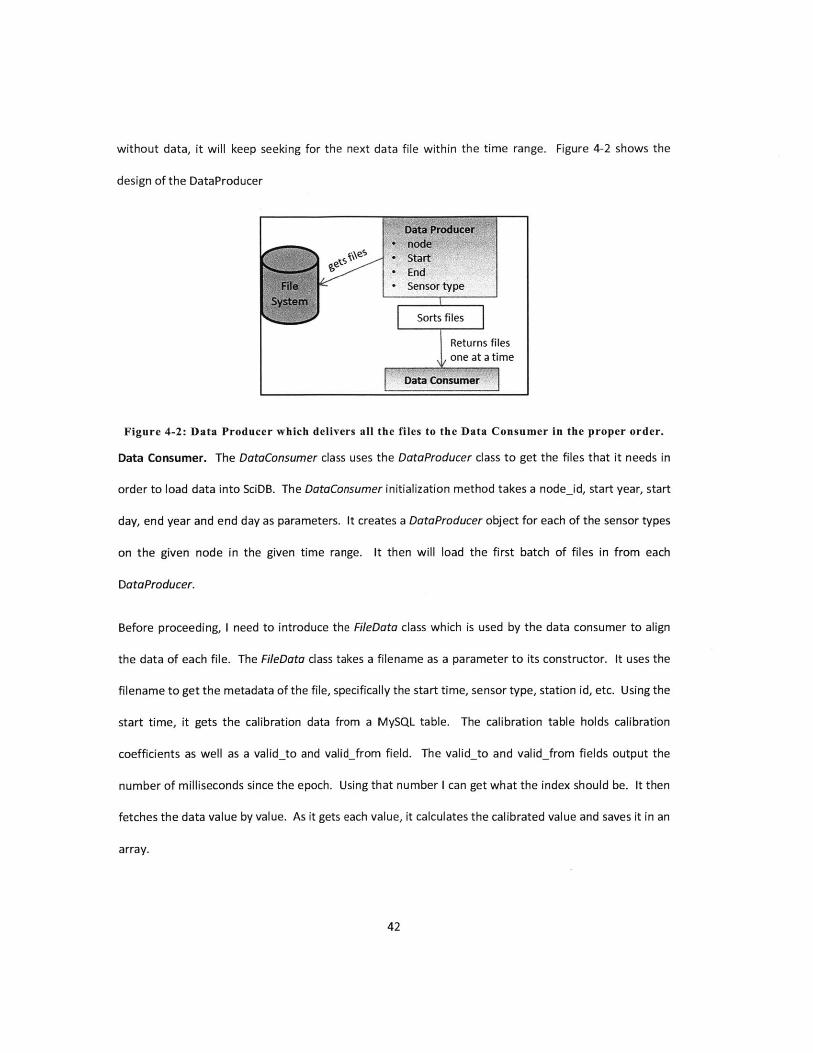
without data, it will keep seeking for the next data file within the time range. Figure 4-2 shows the

design of the DataProducer

\5 -startga6 End

- Sensor type

Sorts files

Returns filesone at a time

Figure 4-2: Data Producer which delivers all the files to the Data Consumer in the proper order.

Data Consumer. The DataConsumer class uses the DataProducer class to get the files that it needs in

order to load data into SciDB. The DataConsumer initialization method takes a node_id, start year, start

day, end year and end day as parameters. It creates a DataProducer object for each of the sensor types

on the given node in the given time range. It then will load the first batch of files in from each

DataProducer.

Before proceeding, I need to introduce the FileData class which is used by the data consumer to align

the data of each file. The FileData class takes a filename as a parameter to its constructor. It uses the

filename to get the metadata of the file, specifically the start time, sensor type, station id, etc. Using the

start time, it gets the calibration data from a MySQL table. The calibration table holds calibration

coefficients as well as a validto and validfrom field. The validto and validfrom fields output the

number of milliseconds since the epoch. Using that number I can get what the index should be. It then

fetches the data value by value. As it gets each value, it calculates the calibrated value and saves it in an

array.

42

The DataProducer class has method called writeChunk whose purpose is to write the next chunk of data

to a properly formatted SciDB input file and then call a system command to upload that chunk to SciDB.

SciDB expects an ASCII file in the following format:

[[findex,nodeid} (h,phprorp) ... ]

Where index is the time index, nodeid is the node number, h is the Hydrophone value, ph is the PH

calibrated value, pr is the calibrated pressure value, orp is the ORP calibrated value. If any field is null

(for example most of the ORP and PH entries) then a question mark is placed there representing null in

SciDB.

The WriteChunk method writes all of the data for one chunk into a file. The DataConsumer then runs an

import command to put the contents of that file into SciDB.

The pseudo code for the loop is as follows:

f ile. write(" [ [")#Make sure we are still in the chunk and have dataWhile curIndex<maxIndex and curIndex!=None:

data= [,?, ?, ?]for each sensor:

if sensor has data at curIndex:add data to the correct spot in the data array# Now we must check to make sure we don't need to# load data into any of the arraysif sensor out of data:

load data into arrayfile.write("{curIndex,nodeid} (p,ph,pr,orp)")curIndex=minimum index of the next value in of the sensor arrays

f.write("]]")

43

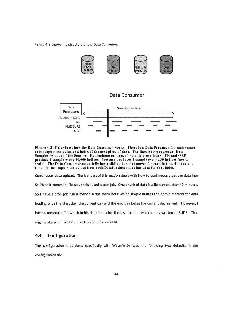
Figure 4-3 shows the structure of the Data Consumer.

Data Consumer

DataProducers

HYDROPHONEPH

PRESSUREORP

Samples overtime

mm-~~. ....

""" "" -""

m.. .. .m

-... -.~.""" ""

-~ -= m

Figure 4-3: This shows how the Data Consumer works. There is a Data Producer for each sensorthat outputs the value and index of the next piece of data. The lines above represent DataSamples by each of the Sensors. Hydrophone produces 1 sample every index. PH and ORPproduce 1 sample every 60,000 indices. Pressure produces 1 sample every 250 indices (not toscale). The Data Consumer essentially has a sliding bar that moves forward in time -1 index at atime. It then inputs the values from each DataProducer that has data for that index.

Continuous data upload. The last part of this section deals with how to continuously get the data into

SciDB as it comes in. To solve this I used a cron job. One chunk of data is a little more than 49 minutes.

So I have a cron job run a python script every hour which simply utilizes the above method for data

loading with the start day, the current day and the end day being the current day as well. However, I

have a metadata file which holds data indicating the last file that was entirely written to SciDB. That

way I make sure that I start back up on the correct file.

4.4 Configuration

The configuration that deals specifically with WaterWiSe uses the following two defaults in the

configuration file.

44

> SENSORTYPES Defaults to: ["HYDROPHONE","PH","PHORP","PRESSURE","ORP"]

> CHUNKSIZE Defaults to: 1440000

4.5 Sample Data Processing Algorithm

In the course of testing this system, I wanted to put it to use with an operation that would typically be

executed. WaterWiSe does a lot of signal analysis on the signals from the sensors. As I mentioned

before, there are a lot of scientists examining the data, and each one of them creates their own schemes

of accessing and analyzing the data. Various programming languages and algorithms are used in these

analyses.

SciDB currently only has an API for python to access its arrays, but there are plans to extend that API to

other languages such as C, C++, and R.

Mudasser Iqbal has developed an algorithm that is used to detect various events given a signal. He

develops in R and fetches the raw data files from the server and calibrates the values using his own

scripts.

The algorithm has a training phase and the actual analysis phase. The two phases are nearly identical

except that the analysis phase uses the data from the training phase. The algorithm takes the signal and

performs a series of transforms on the vector to produce a resultant vector which contains only the

events that are detected. The events are usually major leaks which results in a steep decline, followed

by steady incline in the signal. The pipeline for the process is shown in Figure 4-4. The input array is

broken into smaller chunks, the first for training and the rest for analysis. The training chunk gets

transformed by the CalcMagnitude function which finds the local minima and local maxima of the array,

everything else becomes a zero. The resulting vector is passed into the FilterDropsAfterRises function

45

which eliminates major drops that occur after major inclines, or drops that don't bring the pressure level

below a standard baseline. The resulting vector is passed to the CalcZScores function which assigns a

score to all remaining values which reduces the weight of increases, and magnifies the weight of

declines. Finally, the array is passed into the DetectBaselineChange function which identifies amplitude

of the events that occur. The training array is passed into the CalculateTolerance function which

basically gets the biggest drop and uses that value as a threshold for any events that occur in the input

signal.

Training,Data

CalcMagnitude()CalcMagnitude()

Cusumdrates()

FilterDropsAfterRises(

P, ICalcZscores()

DetectBaselineChange(

CalculateTolerance()

Figure 4-4: Mudasser Iqbal's MaxDrop algorithm pipeline.

This Algorithm was a good candidate to use with this system for a three main reasons. First, it requires

access to a lot of data, second, it performs substantial calculations on that data, and third, it produces

46

'

several intermediate arrays. An example of how Mudasser would use this system is as follows. First

Mudasser writes a python script, then logs in and uploads the script to the server. The server queues,

and then executes the script. Mudasser can log out and log in and check the status of the job at any

time. Once the job is done, Mudasser can user the resultant SciDB arrays in future calculations or log in

to an interactive shell session to view the contents of the array. This is just an example of how SciDB has

simplified the process of accessing and analyzing the WaterWiSe data.

47

Chapter 5 Analysis

The most important aspect of this tool is the ability to quickly read and write from SciDB. The

performance analysis will therefore focus on this aspect of the tool. Below I will explain the process I

went through to analyze the performance of reading and writing from SciDB, as well as the results that

followed.

5.1 Experiment Set Up

I started by testing the performance of fetching an array, as a function of array query length and chunk

size. For this purpose, I created 20 arrays, one for each combination of the four sensors (PH, ORP,

Pressure, and Hydrophone) and five different array sizes (60000, 240000, 960000, 1920000, 7680000).

Each array had one day's worth of data for three nodes as seen in Table 5-1. All chunks were 1 node

wide.

0 <Attr> ... <Attr>

1 <Attr>

2 <Attr>

172800000 <Attr> ... <Attr>

Table 5-1: The tables I used for the analysis looked like this table.The indicies went from 0 to 172800000, (There are 172800000indices per day). The nodeid included 17,19 and 20. There was oneattribute at each location, whose attribute was one ofPH,ORP,PRESSURE, and HYDROPHONE. There were six copiesof each table, each with different chunk sizes.

The 20 test arrays were named according to the sensor type and the chunk size. For example

"PH60000" is structured as in Table 5-1 with a chunk size of 60000. The arrays I created are listed in

Table 5-2 below.

48

Table Name ChunkSize Attribute

HYDROPHONE60000 60000 HYDROPHONE

HYDROPHONE240000 240000 HYDROPHONE

HYDROPHONE960000 960000 HYDROPHONE

HYDROPHONE1920000 1920000 HYDROPHONE

HYDROPHONE7680000 7680000 HYDROPHONE

ORP60000 60000 ORP

ORP240000 240000 ORP

ORP960000 960000 ORP

ORP1920000 1920000 ORP

ORP7680000 7680000 ORP

PH60000 60000 PH

PH240000 240000 PH

PH960000 960000 PH

PH1920000 1920000 PH

PH7680000 7680000 PH

PRESSURE60000 60000 PRESSURE

PRESSURE240000 240000 PRESSURE

PRESSURE960000 960000 PRESSURE

PRESSURE1920000 1920000 PRESSURE

PRESSURE7680000 7680000 PRESSURE

Table 5-2: A list of the tables created for the analysis

5.2 Experiment Execution

To perform the experiments in this work, we ran a script over each of the arrays and measured the time

required to complete different components of the script. This script issured queries to an array that

requested all of the data in sequence. The amount of data requested in each query was varied during

this experiment.

The amount of data requested in the query ranged in six increments from one quarter of a chunk to 10

chunks: 0.25, 0.5, 1, 2, 5, and 10 chunks.

Since these tests would eventually read from each table multiple times, it is important to eliminate

caching effects. To address this, we ran the tests in groups that ran once on each of the 20 test arrays.

Then, before running the next group, we shut down SciDB and cleared the OS block cache.

49

This process is summarized as:

e Start up SciDB

e Query all of the data in all 20 of the tables with a certain query size.

e Shut down SciDB

e Clear the block cache

e Increment query size

e Repeat

With every query I recorded which table I was querying, which node, the starting index, the ending

index, the chunk size of the table, how long it takes to request the data (i.e. the execute query() call to

SciDB), and how long it takes to iterate over the data in Python.

5.3 Experimental Results

I was interested in knowing how effective SciDB with my tool would be at accessing the data. To put it

in perspective I wanted to test the baseline performance of the disk by reading and writing zeros to a

file. I used the unix command dd as follows:

dd if=/dev/zero of=./zeroFile bs=1024 count=1000000

This reads 1,000,000 kilobytes of zeros to an output file named zeroFile. I repeated this four times to

different files at different times. The resultant speeds were 162 MB/s, 196 MB/s, 252 MB/s, and 255

MB/s for an average of 216.25 MB/s for writing.

To test the reading speed I used:

dd if=zeroFile of=/dev/null bs=1024 count=1000000

50

This reads 1,000,000 kilobytes from file zeroFile and dumps what it reads. The resultant speeds of the

four iterations were 106 MB/s, 103 MB/s, 104 MB/s and 104 MB/s for an average of 104.75 MB/s.

5.3.1 Results of querying one quarter of a chunk

Since I queried the data sequentially, I wanted to see how fast the first query performed in comparison

to the next three queries that should be hitting data that had already been loaded in the first query. So,

looking at the data, I set the chunk size to be constant and the query size to be one quarter of a chunk. I

looked at the speed of the query against the first index of the query. As predicted the first query was

much slower than the following three.

Request Time By Index

OCr

- . + ++ ++ ++ ++ ++ +++++ ++ ++ + +Request Time By Index

L

1E0.1

00

U

-4000000 1000000 6000000 11000000 16000000 21000000

Adjusted Index (213926400000->0)

Figure 5-1: PRESSURE1920000, with reads of %4 the size of a chunk on node 17. The index isadjusted where index 213926400000 -> 0 This data is from 22 May 2011.

The first query of a chunk took on average 0.24 seconds while the rest took on average 0.12 seconds. In

this example each chunk contains 240K four-byte floating point values, for a total of 960 KB of data. If

we amortize the cost of loading the chunk over the 4 queries that process the data, we get a total of

0.94 MB of data processed in 0.60 seconds which amounts to 1.6 MVB/s aggregate throughout.

51

Breaking down this performance even further, we can compute separate throughput numbers for the

SciDB chunk read and the SciDB query processing speed. In this analysis we make an assumption that

the work to process the query occurs after the chunk read completes. If this is the case, then we can

deduct the typical processing time of 0.12 seconds from the 'read chunk' time of 0.24 seconds, and

conclude that the chunk is read from disk into SciDB in 0.12 seconds, yielding 7.8 MB/s throughput,

while the query processing portion of the process takes a total of 4*0.12 seconds, yielding 2.0 MB/s

throughput for that portion of the process.

To corroborate these results, we also looked at data from the same pressure data, with a larger chunk

size. With a chunk size of 7,680,000 the first query of each chunk took on average 1.18 seconds, the last

three took on average 0.54 seconds. Here each chunk contains 960K four-byte floating point values, for

a total of 3.84 MB of data. Amortizing these numbers across the four queries gives 3.84 MB processed

in 2.8 seconds, which shows 1.4 MB/s aggregate throughput. These results are found in Figure 5-2.

Pressure Chunk: 7680000

Sam NU o

55000000 650D000 75000000 85000000 95000000index

Figure 5-2: Pressure query results with chunk size of 7680000.

52

I8

1.2

1

0.8

0.6

0.4

0.2

0

*Pressure Chunk:7680000

5.3.2 Performance for long arrays.I also wanted to see how these arrays performed for querying small amounts of data vs. querying large

amounts of data. Ideally, queries would be able to scale linearly when fetching larger data sets. I found

that the query time does scale linearly with length, as shown in Figure 5-3. The throughput rate for this

test comes to 1.76 MB/s which correlates well with our previous data.

44

- length01 3 Average Request time byE

-4 --- ir e lengt

2 T - Linear (Average Requestr_ ~ ~ -time by length)

1 -

00 5000000 10000000 15000000 20000000

Array Length in Indices

Figure 5-3: Average request time vs. length of dataset. Generated using PRESSURE data.

I was also interested in the variance in the speeds of the results. It is intuitive to think that the longer

queries will have greater variance in the requests speeds. Figure 5-4 shows that the shorter queries

performed very similarly, while longer queries varied in length considerably. It is also interesting to note

that of the queries that searched over almost 19,000,000 indices, the slower ones had smaller chunk

sizes resulting in more chunks being accessed. Conversely, the faster queries were the ones that had

larger chunks, thus accessing more relevant data.

53

4.' I ~--------__________ __ -.GD 10 -4- --

0. ___ ______ $ __

~..J TY~ -T - - ~~~~~1

0 5000000 10000000 15000000 20000000 25000000

Adjusted Index

Figure 5-4: The raw values showing longer queries have greater variance in performance.

5.3.3 SciDBIterator.After loading each query, I also iterated over every element in the iterator in the Python script. I did not

perform any operations on each element because I wanted to see the performance specifically of the

iterator. We found that the throughput in this case was 15K pressure values per second. This

demonstrates the extremely high cost of iterating in Python. I suspected that the more chunks that

were accessed in a query would decrease the performance of the iterator as there is more overhead in

switching out the chunk for the a new chunk in the SciDBiterator would slow down the operation. What

I found instead was a nearly perfectly linear result, where the time spent iterating was directly

proportional to the amount of data in the iterator, with no obvious overhead from swapping chunks.

See Figure 5-5 for results. The largest query spanned 10 chunks while the smallest query spanned .25

chunks.

54

14

12

10

8

a.6

w40

2

* Series1

Figure 5-5: Performance of iterating over every element of an array. Amount of data vs. Latencyshows the length of the data is linearly proportional to the latency of iteration.

5.4 Discussion

In this analysis, our goal was to understand how our implementation performed, and how we might

improve performance by tuning the interface to SciDB. In this study we made two key

observations. First, we observed that the performance bottleneck in the system is not raw disk 1/0, but

rather other processing that occurs between when SciDB loads a chunk and when an iterator object is

instantiated in Python. Second, we observed that there is a non-negligible performance cost to using

sparse arrays.

The SciDB/Python bottleneck might be explained by delving into the code that implements it. This

feature is a relatively recent addition to the system, and it may not be fully optimized. Alternatively,

there might be a much more efficient way of extracting the data needed for our specific application by

building our own customized Python connector. We would like to be able to operate using the NumPy

toolkit, and thus pull data out of SciDB into a NumPy array. This cannot be done efficiently with the

current Python interface.

55

Iteration Speed

-- - -9 -- - - - -- - --- 4 --

70

60- 4

_0_+_Iteration

___Speed30

20A

-4000000 1000000 6000000 11000000

Length of Array

Another cause for the reduction in performance might have to do with the way we are structuring the

data in SciDB. Each of our arrays contained data for a single sensor type and each sample of data was

represented as an attribute on a particular cell. Further, we defined a single global sample counter at 2

KHz, and represented all of the data streams at that rate, even if they were sampled at lower rates. For

example, Pressure data was sampled at 250 Hz, but it is represented in a sparse array that has 2000

indices per second. Therefore, only one cell in 8 is actually in use. ORP and pH data is even more

extreme, with samples taken only every minute. Our experiments comparing Hydrophone data (which

operates at full rate) and Pressure data (operating at 1/8 rate) suggest that there is a non-negligible

overhead in skipping the additional data elements. Unfortunately, we did not have time to experiment

with other schemas. Good choices for future work would be to test single arrays with multiple sensor

attributes per cell, or separate arrays with a different indexing scheme.

56

Chapter 6 Future Work

This project is a prototype and a first version product. It has not had the benefit of being used a large

community of users to work out all the bugs. I have thought of several ways to extend and improve the

tool that fell outside the scope of this project. This section enumerates most of the ideas that have

occurred throughout the course of this project.

6.1 Security and Authentication

Security wasn't a major focus of this project, but definitely needs to be addressed. The simplest thing

that can be done is to use the server's users and passwords. UNIX already has a methodology for

handling user accounts, passwords, and permissions. There is no need to redevelop something that has

been created and well tested.

The system as it now stands is vulnerable to man-in-the-middle attacks where an adversary can

intercept messages from either the client or the server and can easily imitate either. This can be

avoided by using the SSH protocol between the client and server. Each message would be encrypted

with secret keys known only be the client and server. These two methods would secure access to the

server and prevent most adversaries from attacking the server.

The server is still very vulnerable to malicious users. This system allows users to execute arbitrary

commands and upload files to the server. The possibilities are almost endless for attackers in this

scenario. To overcome these security vulnerabilities the system administrator can set the user

permissions for the user running the server to only have access to this tools root directory and no other

files on the computer. One could also sandbox all of the scripts that are uploaded as well as any other

possibility for an attacker to run arbitrary code. Furthermore, any input taken from a user should be

sanitized to ensure the input is not trying to perform some malicious action.

57

The MySQL tables are all vulnerable to attacks such as SQL injection attacks. Sanitizing input would

certainly help to prevent this kind of attack, but for added security it would be wise to change the

permissions of the user that access the SQL database. Presently, the user is root with full access.

6.2 Garbage Collection

The garbage collection scheme I used is very simplistic, which has its merits, but more intelligent things

could be done. I garbage collect based only on least recently used array and a maximum disk utilization.

In many instances this system works just fine. The biggest problem with having a maximum array count

is that it is foreseeable that a user could require more than the maximum array count for a particular

algorithm. In that case, the system would likely crash as it would garbage collect arrays that it is

currently using and fall into a cycle of continuously reloading and garbage collecting all of the arrays.

Solutions I could imagine include using a combination of array count and disk capacity barriers. Also, it

would be useful to design a system where each array is given a priority and the lower priority arrays are

garbage collected sooner.

6.3 Parallelization

SciDB has built in cloud computing functionality. It wouldn't take much to extend this system to work on

a cloud. This would allow for much quicker calculations and results.

6.4 Logging

I developed a logging system that will log any message with any status. It logs the time, the status and

the level. I also developed a system to query and filter the logs, so as to be able to diagnose problems

quickly. I was unable to integrate this system into the tool, but I have packaged it with the tools. In the

future developers can integrate the logger putting log statements where they deem prudent and can

then track any bug or other problem in the software.

58

6.5 Graphical User Interface

This work lends itself well for visualization and graphical representations of data. Furthermore, software

systems generally gain more traction if they have graphical user interfaces as they are generally more

intuitive to use. There are endless possibilities for different interfaces that would facilitate the viewing

of data, reporting the progress of jobs, and otherwise assisting users.

6.6 Data import to SciDB

As I said earlier, it is quite slow to write arrays to disk then import them to SciDB from disk. SciDB has

plans to create this functionality but they are very busy dealing with an ever growing and in demand

product.

59

Chapter 7 Related Work

In the past couple of years datasets have grown significantly and the desire to analyze large amounts of

data has prompted several new concepts in databases. Below I name some companies and products

whose work has parallels with the work explained in this paper.

7.1 NumPy

NumPy is a python library developed for mathematical and scientific calculations. It has grown into

wide spread use and is the engine that powers a lot of scientific solutions today. NumPy's library is

expansive including capabilities for N-dimensional array objects, linear algebra functions, Fourier

transform functions, and many more. [3] NumPy would be a powerful tool to use in conjunction with

SciDB as NumPy is predominantly an in-memory data solution. The ability to load an array from SciDB

into a NumPy array, perform computations on the array, and saving it to SciDB would prove invaluable

and the foundations to do such are laid out in this work.

NumPy is able to utilize the syntax and simplicity of programming in python while utilizing the higher

performance of C and C++ libraries. This allows calculations on n-dimensional arrays to avoid the

overhead of dealing with an exponential amount of python objects, but rather to perform the

operations quicker in C and C++.

7.2 SciPy

SciPy is a python module built off of NumPy. It specializes in scientific calculation with NumPy's n-array

as the core data type. SciPy would prove very valuable to use in conjunction with SciDB and this tool.

7.4 MATLAB

According to MathWorks' web page,

60

"MATLAB' is a high-level language and interactive environment that enables you to perform

computationally intensive tasks faster than with traditional programming languages such as C,

C++, and Fortran." [7]

That sounds exactly like what I tried to accomplish with this project. I wanted to enable an interactive

environment to perform computationally intensive tasks. SciDB specifically focusses on storing large

databases on disk where this is a weakness of MATLAB.

7.5 Ipython

Ipython is a python toolkit used to enable interactive shell including tools for parallel computing,

visualization, and GUI toolkits. [8] As I mentioned in the future works section, WaterWiSe would benefit

from developing a Graphical User Interface with visualization and parallelization. lpython doesn't

necessarily offer any specific tools for big data analysis.

61

Chapter 8 Conclusion

The software design project discussed in this document describes a software system developed for

WaterWiSe that facilitates remote data access for very large scientific data. WaterWiSe is a project

involved with sensing and analyzing the water distribution network in Singapore. The major task

involved in developing the system was the integration of the data with SciDB, a Data Management and

Analytics Software System. I explained how to organize the data within SciDB, how to load the data,

how to extract the data and how to resave the data.

SciDB proved to be invaluable in this process as it exposes most of the functionality that was desired by

WaterWiSe and provided the flexibility to achieve other functionality that was not readily available.

This tool also provides remote access to the data by users who use the data for signal processing and

monitoring. Users can upload a python script which will be executed accessing and manipulating the

high resolution data generated by the system's sensor network.

62

Bibliography

[1] "center for environmental sensing and modeling," 2008. [Online]. Available:

http://censam.mit.edu/about/index.html. [Accessed 19 10 2011].

[2] "URBAN HYDROLOGY & WATER RESOURCES," censam, [Online]. Available:

http://censam.mit.edu/research/res2/index.html#sec1. [Accessed 6 2 2012].

[3] "What is NumPy?," SciPy, 2008. [Online]. Available:

http://docs.scipy.org/doc/numpy/user/whatisnumpy.html. [Accessed 6 2 2012].

[4] "Vertica: Customers," Vertica, 2011. [Online]. Available: http://www.vertica.com/customers/.

[Accessed 42 2012].

[5] J. B. D. D. e. a. Michael Stonebracker, "Requirements for Science Data Bases and SciDB," 2009.

[6] Vertica, "Fast Data Loading into Vertica Analytic Database".

[7] MATLAB, "MATLAB - The Language of Technical Computer," MATLAB, 2012. [Online]. Available:

http://www.mathworks.com/products/matlab/. [Accessed 4 2 2012].

[8] "IPython: Productive Interactive Computing," IPython, 2012. [Online]. Available: http://ipython.org/.

[Accessed 3 2 2012].

63