Embed Size (px)
Citation preview

ibm.com/redbooks
Front cover
IBM b-type Gen 5 16 Gbps Switches and Network Advisor
Jon TateKameswara Bhaskarabhatla
Bruno Garcia GallePaulo Neto
Learn about the new features of the IBM b-type Gen 5 16 Gbps switches
Read about IBM Network Advisor and Fabric Vision
Learn about preferred practices and troubleshooting tips


International Technical Support Organization
IBM b-type Gen 5 16 Gbps Switches and Network Advisor
May 2014
SG24-8186-00

© Copyright International Business Machines Corporation 2014. All rights reserved.Note to U.S. Government Users Restricted Rights -- Use, duplication or disclosure restricted by GSA ADP ScheduleContract with IBM Corp.
First Edition (May 2014)
This edition applies to IBM Network Advisor V12 and FOS V7.2, and the IBM b-type Gen 5 16 Gbps switches and directors that are available at the time of writing.
Note: Before using this information and the product it supports, read the information in “Notices” on page vii.
Contents
Notices . . . . . . . . . . . . . . . . . . . . . . . . . . . . . . . . . . . . . . . . . . . . . . . . . . . . . . . . . . . . . . . . . viiTrademarks . . . . . . . . . . . . . . . . . . . . . . . . . . . . . . . . . . . . . . . . . . . . . . . . . . . . . . . . . . . . . viii
Preface . . . . . . . . . . . . . . . . . . . . . . . . . . . . . . . . . . . . . . . . . . . . . . . . . . . . . . . . . . . . . . . . . ixAuthors. . . . . . . . . . . . . . . . . . . . . . . . . . . . . . . . . . . . . . . . . . . . . . . . . . . . . . . . . . . . . . . . . . ixNow you can become a published author, too! . . . . . . . . . . . . . . . . . . . . . . . . . . . . . . . . . . . xiComments welcome. . . . . . . . . . . . . . . . . . . . . . . . . . . . . . . . . . . . . . . . . . . . . . . . . . . . . . . . xiStay connected to IBM Redbooks . . . . . . . . . . . . . . . . . . . . . . . . . . . . . . . . . . . . . . . . . . . . . xi
Chapter 1. Product introduction . . . . . . . . . . . . . . . . . . . . . . . . . . . . . . . . . . . . . . . . . . . . 11.1 Overview of the product . . . . . . . . . . . . . . . . . . . . . . . . . . . . . . . . . . . . . . . . . . . . . . . . . 2
1.1.1 Hardware features . . . . . . . . . . . . . . . . . . . . . . . . . . . . . . . . . . . . . . . . . . . . . . . . . 21.1.2 Brocade Fabric Vision technology. . . . . . . . . . . . . . . . . . . . . . . . . . . . . . . . . . . . . . 21.1.3 Fabric OS features . . . . . . . . . . . . . . . . . . . . . . . . . . . . . . . . . . . . . . . . . . . . . . . . . 31.1.4 Hardware naming convention: IBM and Brocade . . . . . . . . . . . . . . . . . . . . . . . . . . 51.1.5 Fabric Operating System hardware support . . . . . . . . . . . . . . . . . . . . . . . . . . . . . . 61.1.6 Management . . . . . . . . . . . . . . . . . . . . . . . . . . . . . . . . . . . . . . . . . . . . . . . . . . . . . . 61.1.7 Monitoring . . . . . . . . . . . . . . . . . . . . . . . . . . . . . . . . . . . . . . . . . . . . . . . . . . . . . . . . 61.1.8 IBM Network Advisor. . . . . . . . . . . . . . . . . . . . . . . . . . . . . . . . . . . . . . . . . . . . . . . . 7
1.2 Product descriptions . . . . . . . . . . . . . . . . . . . . . . . . . . . . . . . . . . . . . . . . . . . . . . . . . . . . 71.2.1 IBM System Networking SAN24B-5 . . . . . . . . . . . . . . . . . . . . . . . . . . . . . . . . . . . . 71.2.2 IBM System Networking SAN48B-5 . . . . . . . . . . . . . . . . . . . . . . . . . . . . . . . . . . . . 91.2.3 IBM System Networking SAN96B-5 . . . . . . . . . . . . . . . . . . . . . . . . . . . . . . . . . . . 101.2.4 IBM System Networking SAN384B-2 and IBM System Networking SAN768B-2 . 12
Chapter 2. Product hardware and features . . . . . . . . . . . . . . . . . . . . . . . . . . . . . . . . . . . 172.1 Topologies. . . . . . . . . . . . . . . . . . . . . . . . . . . . . . . . . . . . . . . . . . . . . . . . . . . . . . . . . . . 18
2.1.1 Edge-core topology. . . . . . . . . . . . . . . . . . . . . . . . . . . . . . . . . . . . . . . . . . . . . . . . 182.1.2 Edge-core-edge topology . . . . . . . . . . . . . . . . . . . . . . . . . . . . . . . . . . . . . . . . . . . 192.1.3 Full-mesh topology . . . . . . . . . . . . . . . . . . . . . . . . . . . . . . . . . . . . . . . . . . . . . . . . 19
2.2 Gen 5 Fibre Channel technology . . . . . . . . . . . . . . . . . . . . . . . . . . . . . . . . . . . . . . . . . 192.2.1 Condor3 ASIC. . . . . . . . . . . . . . . . . . . . . . . . . . . . . . . . . . . . . . . . . . . . . . . . . . . . 192.2.2 Fabric Vision . . . . . . . . . . . . . . . . . . . . . . . . . . . . . . . . . . . . . . . . . . . . . . . . . . . . . 20
2.3 IBM System Networking SAN b-type family . . . . . . . . . . . . . . . . . . . . . . . . . . . . . . . . . 272.4 IBM System Networking Gen 5 SAN b-type family . . . . . . . . . . . . . . . . . . . . . . . . . . . . 28
2.4.1 IBM System Networking SAN24B-5 (2498-F24, 2498-X24, and 2498-24G) . . . . 282.4.2 IBM System Networking SAN48B-5 (2498-F48) . . . . . . . . . . . . . . . . . . . . . . . . . . 302.4.3 IBM System Networking SAN96B-5 (2498-F96 / 2498-N96) . . . . . . . . . . . . . . . . 332.4.4 IBM System Networking SAN384B-2 (2499-416) and IBM System Networking
SAN768B-2 (2499-816) . . . . . . . . . . . . . . . . . . . . . . . . . . . . . . . . . . . . . . . . . . . . 362.4.5 IBM Fabric backbone blades . . . . . . . . . . . . . . . . . . . . . . . . . . . . . . . . . . . . . . . . 402.4.6 Optical UltraScale Inter-Chassis Links . . . . . . . . . . . . . . . . . . . . . . . . . . . . . . . . . 49
2.5 Generic features . . . . . . . . . . . . . . . . . . . . . . . . . . . . . . . . . . . . . . . . . . . . . . . . . . . . . . 572.5.1 Zoning . . . . . . . . . . . . . . . . . . . . . . . . . . . . . . . . . . . . . . . . . . . . . . . . . . . . . . . . . . 572.5.2 ISL Trunking . . . . . . . . . . . . . . . . . . . . . . . . . . . . . . . . . . . . . . . . . . . . . . . . . . . . . 572.5.3 Dynamic Path Selection . . . . . . . . . . . . . . . . . . . . . . . . . . . . . . . . . . . . . . . . . . . . 602.5.4 Port types . . . . . . . . . . . . . . . . . . . . . . . . . . . . . . . . . . . . . . . . . . . . . . . . . . . . . . . 612.5.5 In-flight encryption and compression . . . . . . . . . . . . . . . . . . . . . . . . . . . . . . . . . . 612.5.6 NPIV . . . . . . . . . . . . . . . . . . . . . . . . . . . . . . . . . . . . . . . . . . . . . . . . . . . . . . . . . . . 62
© Copyright IBM Corp. 2014. All rights reserved. iii

2.5.7 Dynamic Fabric Provisioning. . . . . . . . . . . . . . . . . . . . . . . . . . . . . . . . . . . . . . . . . 63
Chapter 3. IBM Network Advisor . . . . . . . . . . . . . . . . . . . . . . . . . . . . . . . . . . . . . . . . . . . 653.1 Planning server and client system requirements . . . . . . . . . . . . . . . . . . . . . . . . . . . . . 66
3.1.1 Server and client operating system and hardware requirements . . . . . . . . . . . . . 663.1.2 Client and server system requirements. . . . . . . . . . . . . . . . . . . . . . . . . . . . . . . . . 683.1.3 Browser requirements for IBM Network Advisor . . . . . . . . . . . . . . . . . . . . . . . . . . 693.1.4 Supported Fabric OS versions with IBM Network Advisor V12.0.x. . . . . . . . . . . . 693.1.5 Recommended upgrade path and supported Fabric OS . . . . . . . . . . . . . . . . . . . 693.1.6 Enterprise Fabric Connectivity Manager upgrade path to IBM Network Advisor target
path. . . . . . . . . . . . . . . . . . . . . . . . . . . . . . . . . . . . . . . . . . . . . . . . . . . . . . . . . . . . 703.1.7 Downloading software. . . . . . . . . . . . . . . . . . . . . . . . . . . . . . . . . . . . . . . . . . . . . . 703.1.8 Pre-installation requirements . . . . . . . . . . . . . . . . . . . . . . . . . . . . . . . . . . . . . . . . 713.1.9 Syslog troubleshooting . . . . . . . . . . . . . . . . . . . . . . . . . . . . . . . . . . . . . . . . . . . . . 72
3.2 New installations and upgrading IBM Network Advisor to Version 12.0.3. . . . . . . . . . . 723.2.1 New installation of IBM Network Advisor . . . . . . . . . . . . . . . . . . . . . . . . . . . . . . . 733.2.2 Upgrading to IBM Network Advisor V12.0.x from an existing IBM Network Advisor
installation. . . . . . . . . . . . . . . . . . . . . . . . . . . . . . . . . . . . . . . . . . . . . . . . . . . . . . . 933.3 User, device, and dashboard management . . . . . . . . . . . . . . . . . . . . . . . . . . . . . . . . 101
3.3.1 User management . . . . . . . . . . . . . . . . . . . . . . . . . . . . . . . . . . . . . . . . . . . . . . . 1013.3.2 Discovering and adding SAN fabrics. . . . . . . . . . . . . . . . . . . . . . . . . . . . . . . . . . 108
3.4 New features of IBM Network Advisor V12.0.3 . . . . . . . . . . . . . . . . . . . . . . . . . . . . . . 1163.4.1 Performance Dashboard. . . . . . . . . . . . . . . . . . . . . . . . . . . . . . . . . . . . . . . . . . . 1163.4.2 Frame Viewer . . . . . . . . . . . . . . . . . . . . . . . . . . . . . . . . . . . . . . . . . . . . . . . . . . . 1173.4.3 Port Commissioning . . . . . . . . . . . . . . . . . . . . . . . . . . . . . . . . . . . . . . . . . . . . . . 1173.4.4 Bulk Port Configuration . . . . . . . . . . . . . . . . . . . . . . . . . . . . . . . . . . . . . . . . . . . . 118
3.5 IBM Network Advisor Dashboard . . . . . . . . . . . . . . . . . . . . . . . . . . . . . . . . . . . . . . . . 1193.5.1 Dashboard overview . . . . . . . . . . . . . . . . . . . . . . . . . . . . . . . . . . . . . . . . . . . . . . 1193.5.2 Customizing the dashboard . . . . . . . . . . . . . . . . . . . . . . . . . . . . . . . . . . . . . . . . 1203.5.3 Performance Dashboard. . . . . . . . . . . . . . . . . . . . . . . . . . . . . . . . . . . . . . . . . . . 121
3.6 Scheduling daily or weekly backups for the fabric configuration. . . . . . . . . . . . . . . . . 1253.6.1 Call Home . . . . . . . . . . . . . . . . . . . . . . . . . . . . . . . . . . . . . . . . . . . . . . . . . . . . . . 126
3.7 Fabric Vision . . . . . . . . . . . . . . . . . . . . . . . . . . . . . . . . . . . . . . . . . . . . . . . . . . . . . . . . 1293.7.1 ClearLink Diagnostics . . . . . . . . . . . . . . . . . . . . . . . . . . . . . . . . . . . . . . . . . . . . . 1303.7.2 Bottleneck Detection . . . . . . . . . . . . . . . . . . . . . . . . . . . . . . . . . . . . . . . . . . . . . . 1303.7.3 Flow Vision . . . . . . . . . . . . . . . . . . . . . . . . . . . . . . . . . . . . . . . . . . . . . . . . . . . . . 1313.7.4 Monitoring Alerting Policy Suite . . . . . . . . . . . . . . . . . . . . . . . . . . . . . . . . . . . . . 1343.7.5 Simplified management and reporting . . . . . . . . . . . . . . . . . . . . . . . . . . . . . . . . 1353.7.6 Investment protection . . . . . . . . . . . . . . . . . . . . . . . . . . . . . . . . . . . . . . . . . . . . . 135
3.8 Using MAPS with IBM Network Advisor . . . . . . . . . . . . . . . . . . . . . . . . . . . . . . . . . . . 1353.8.1 Configuring MAPS by using IBM Network Advisor . . . . . . . . . . . . . . . . . . . . . . . 1363.8.2 Configuring MAPS actions . . . . . . . . . . . . . . . . . . . . . . . . . . . . . . . . . . . . . . . . . 1383.8.3 Creating policies and rules . . . . . . . . . . . . . . . . . . . . . . . . . . . . . . . . . . . . . . . . . 139
3.9 Configuring Flow Vision using IBM Network Advisor . . . . . . . . . . . . . . . . . . . . . . . . . 1403.9.1 Adding a flow definition . . . . . . . . . . . . . . . . . . . . . . . . . . . . . . . . . . . . . . . . . . . . 141
Chapter 4. Initial switch setup and configuration . . . . . . . . . . . . . . . . . . . . . . . . . . . . 1434.1 Initial setup . . . . . . . . . . . . . . . . . . . . . . . . . . . . . . . . . . . . . . . . . . . . . . . . . . . . . . . . . 144
4.1.1 Configuring the IBM System Storage fabric backbone . . . . . . . . . . . . . . . . . . . . 1444.1.2 IBM System Storage b-type switch initial configuration . . . . . . . . . . . . . . . . . . . 1474.1.3 EZSwitchSetup initial configuration. . . . . . . . . . . . . . . . . . . . . . . . . . . . . . . . . . . 152
Chapter 5. Gen 5 switches and IBM FlashSystem . . . . . . . . . . . . . . . . . . . . . . . . . . . . 1675.1 IBM FlashSystem with IBM Gen 5 directors . . . . . . . . . . . . . . . . . . . . . . . . . . . . . . . . 168
iv IBM b-type Gen 5 16 Gbps Switches and Network Advisor
5.1.1 Introduction to IBM FlashSystem storage systems. . . . . . . . . . . . . . . . . . . . . . . 1685.1.2 IBM FlashSystem portfolio . . . . . . . . . . . . . . . . . . . . . . . . . . . . . . . . . . . . . . . . . 169
5.2 Accessing, connecting, and virtualizing IBM Flash System . . . . . . . . . . . . . . . . . . . . 1705.2.1 Initial setup of IBM FlashSystem. . . . . . . . . . . . . . . . . . . . . . . . . . . . . . . . . . . . . 1705.2.2 Creating logical units on IBM FlashSystem. . . . . . . . . . . . . . . . . . . . . . . . . . . . . 1725.2.3 Modifying volumes . . . . . . . . . . . . . . . . . . . . . . . . . . . . . . . . . . . . . . . . . . . . . . . 1775.2.4 Modifying access to the existing volumes. . . . . . . . . . . . . . . . . . . . . . . . . . . . . . 1795.2.5 Port masking and SAN zoning between IBM SAN Volume Controller and IBM
FlashSystem. . . . . . . . . . . . . . . . . . . . . . . . . . . . . . . . . . . . . . . . . . . . . . . . . . . . 1815.2.6 Creating an MDisk group . . . . . . . . . . . . . . . . . . . . . . . . . . . . . . . . . . . . . . . . . . 183
Chapter 6. Preferred practices . . . . . . . . . . . . . . . . . . . . . . . . . . . . . . . . . . . . . . . . . . . . 1876.1 Physical patching . . . . . . . . . . . . . . . . . . . . . . . . . . . . . . . . . . . . . . . . . . . . . . . . . . . . 188
6.1.1 Using a structured approach. . . . . . . . . . . . . . . . . . . . . . . . . . . . . . . . . . . . . . . . 1886.1.2 Modular cabling. . . . . . . . . . . . . . . . . . . . . . . . . . . . . . . . . . . . . . . . . . . . . . . . . . 1896.1.3 Cabling high-density and high-port count fiber equipment . . . . . . . . . . . . . . . . . 1896.1.4 Using color to identify cables . . . . . . . . . . . . . . . . . . . . . . . . . . . . . . . . . . . . . . . 1906.1.5 Establishing a naming scheme . . . . . . . . . . . . . . . . . . . . . . . . . . . . . . . . . . . . . . 1906.1.6 Patch cables . . . . . . . . . . . . . . . . . . . . . . . . . . . . . . . . . . . . . . . . . . . . . . . . . . . . 1916.1.7 Patch panels . . . . . . . . . . . . . . . . . . . . . . . . . . . . . . . . . . . . . . . . . . . . . . . . . . . . 1916.1.8 Horizontal and backbone cables . . . . . . . . . . . . . . . . . . . . . . . . . . . . . . . . . . . . . 1916.1.9 Horizontal cable managers . . . . . . . . . . . . . . . . . . . . . . . . . . . . . . . . . . . . . . . . . 1916.1.10 Vertical cable managers . . . . . . . . . . . . . . . . . . . . . . . . . . . . . . . . . . . . . . . . . . 1926.1.11 Overhead cable pathways . . . . . . . . . . . . . . . . . . . . . . . . . . . . . . . . . . . . . . . . 1926.1.12 Cable ties . . . . . . . . . . . . . . . . . . . . . . . . . . . . . . . . . . . . . . . . . . . . . . . . . . . . . 1926.1.13 Implementing the cabling infrastructure . . . . . . . . . . . . . . . . . . . . . . . . . . . . . . 1926.1.14 Testing the links . . . . . . . . . . . . . . . . . . . . . . . . . . . . . . . . . . . . . . . . . . . . . . . . 1926.1.15 Building a common framework for the racks . . . . . . . . . . . . . . . . . . . . . . . . . . . 1936.1.16 Preserving the infrastructure. . . . . . . . . . . . . . . . . . . . . . . . . . . . . . . . . . . . . . . 1946.1.17 Documentation . . . . . . . . . . . . . . . . . . . . . . . . . . . . . . . . . . . . . . . . . . . . . . . . . 1946.1.18 Stocking spare cables. . . . . . . . . . . . . . . . . . . . . . . . . . . . . . . . . . . . . . . . . . . . 1946.1.19 Preferred practices for managing cabling . . . . . . . . . . . . . . . . . . . . . . . . . . . . . 1956.1.20 Summary. . . . . . . . . . . . . . . . . . . . . . . . . . . . . . . . . . . . . . . . . . . . . . . . . . . . . . 196
6.2 SAN design basics . . . . . . . . . . . . . . . . . . . . . . . . . . . . . . . . . . . . . . . . . . . . . . . . . . . 1976.2.1 Topologies . . . . . . . . . . . . . . . . . . . . . . . . . . . . . . . . . . . . . . . . . . . . . . . . . . . . . 1976.2.2 Inter-Switch Link . . . . . . . . . . . . . . . . . . . . . . . . . . . . . . . . . . . . . . . . . . . . . . . . . 1976.2.3 Inter-Chassis Links . . . . . . . . . . . . . . . . . . . . . . . . . . . . . . . . . . . . . . . . . . . . . . . 1986.2.4 Device placement . . . . . . . . . . . . . . . . . . . . . . . . . . . . . . . . . . . . . . . . . . . . . . . . 2046.2.5 Fan-in ratios and oversubscription . . . . . . . . . . . . . . . . . . . . . . . . . . . . . . . . . . . 2066.2.6 FCoE as a ToR solution . . . . . . . . . . . . . . . . . . . . . . . . . . . . . . . . . . . . . . . . . . . 2076.2.7 NPIV and the access gateway . . . . . . . . . . . . . . . . . . . . . . . . . . . . . . . . . . . . . . 208
6.3 Data flow considerations . . . . . . . . . . . . . . . . . . . . . . . . . . . . . . . . . . . . . . . . . . . . . . . 2086.3.1 Congestion in the fabric . . . . . . . . . . . . . . . . . . . . . . . . . . . . . . . . . . . . . . . . . . . 2086.3.2 Traffic-based versus frame-based congestion . . . . . . . . . . . . . . . . . . . . . . . . . . 2096.3.3 Sources of congestion . . . . . . . . . . . . . . . . . . . . . . . . . . . . . . . . . . . . . . . . . . . . 2096.3.4 Mitigating congestion with Edge Hold Time . . . . . . . . . . . . . . . . . . . . . . . . . . . . 210
6.4 Redundancy and resiliency . . . . . . . . . . . . . . . . . . . . . . . . . . . . . . . . . . . . . . . . . . . . . 2136.4.1 Single point of failure . . . . . . . . . . . . . . . . . . . . . . . . . . . . . . . . . . . . . . . . . . . . . 215
6.5 Distance . . . . . . . . . . . . . . . . . . . . . . . . . . . . . . . . . . . . . . . . . . . . . . . . . . . . . . . . . . . 2166.5.1 Buffer allocation . . . . . . . . . . . . . . . . . . . . . . . . . . . . . . . . . . . . . . . . . . . . . . . . . 2166.5.2 Fabric interconnectivity over Fibre Channel at longer distances. . . . . . . . . . . . . 2176.5.3 Fibre Channel over IP . . . . . . . . . . . . . . . . . . . . . . . . . . . . . . . . . . . . . . . . . . . . . 2186.5.4 FCIP with FCR . . . . . . . . . . . . . . . . . . . . . . . . . . . . . . . . . . . . . . . . . . . . . . . . . . 220
Contents v
6.5.5 Using EX_Ports and VEX_Ports . . . . . . . . . . . . . . . . . . . . . . . . . . . . . . . . . . . . . 2206.5.6 Advanced FCIP configuration . . . . . . . . . . . . . . . . . . . . . . . . . . . . . . . . . . . . . . . 2226.5.7 FCIP design preferred practices . . . . . . . . . . . . . . . . . . . . . . . . . . . . . . . . . . . . . 2266.5.8 FCIP Trunking. . . . . . . . . . . . . . . . . . . . . . . . . . . . . . . . . . . . . . . . . . . . . . . . . . . 2276.5.9 Virtual Fabrics . . . . . . . . . . . . . . . . . . . . . . . . . . . . . . . . . . . . . . . . . . . . . . . . . . . 2296.5.10 Ethernet Interface Sharing . . . . . . . . . . . . . . . . . . . . . . . . . . . . . . . . . . . . . . . . 2306.5.11 Workloads . . . . . . . . . . . . . . . . . . . . . . . . . . . . . . . . . . . . . . . . . . . . . . . . . . . . . 2316.5.12 Intel -based virtualization storage access . . . . . . . . . . . . . . . . . . . . . . . . . . . . . 232
6.6 Security . . . . . . . . . . . . . . . . . . . . . . . . . . . . . . . . . . . . . . . . . . . . . . . . . . . . . . . . . . . . 2326.6.1 Zone Management: Dynamic Fabric Provisioning (DFP) . . . . . . . . . . . . . . . . . . 2336.6.2 Zone management: Duplicate WWNs. . . . . . . . . . . . . . . . . . . . . . . . . . . . . . . . . 2336.6.3 Role-Based Access Controls . . . . . . . . . . . . . . . . . . . . . . . . . . . . . . . . . . . . . . . 2346.6.4 Default accounts . . . . . . . . . . . . . . . . . . . . . . . . . . . . . . . . . . . . . . . . . . . . . . . . . 2356.6.5 Access control lists . . . . . . . . . . . . . . . . . . . . . . . . . . . . . . . . . . . . . . . . . . . . . . . 2356.6.6 Policy Database Distribution . . . . . . . . . . . . . . . . . . . . . . . . . . . . . . . . . . . . . . . . 2366.6.7 In-flight encryption and compression: b-type (16 Gbps) platforms only . . . . . . . 2366.6.8 In-flight encryption and compression guidelines . . . . . . . . . . . . . . . . . . . . . . . . . 237
6.7 Monitoring . . . . . . . . . . . . . . . . . . . . . . . . . . . . . . . . . . . . . . . . . . . . . . . . . . . . . . . . . . 2386.7.1 Fabric Watch. . . . . . . . . . . . . . . . . . . . . . . . . . . . . . . . . . . . . . . . . . . . . . . . . . . . 2386.7.2 Frame Viewer . . . . . . . . . . . . . . . . . . . . . . . . . . . . . . . . . . . . . . . . . . . . . . . . . . . 2406.7.3 Bottleneck Detection . . . . . . . . . . . . . . . . . . . . . . . . . . . . . . . . . . . . . . . . . . . . . . 2406.7.4 Credit loss . . . . . . . . . . . . . . . . . . . . . . . . . . . . . . . . . . . . . . . . . . . . . . . . . . . . . . 2416.7.5 RAS log. . . . . . . . . . . . . . . . . . . . . . . . . . . . . . . . . . . . . . . . . . . . . . . . . . . . . . . . 2426.7.6 Audit log . . . . . . . . . . . . . . . . . . . . . . . . . . . . . . . . . . . . . . . . . . . . . . . . . . . . . . . 2426.7.7 SAN Health . . . . . . . . . . . . . . . . . . . . . . . . . . . . . . . . . . . . . . . . . . . . . . . . . . . . . 2426.7.8 Design guidelines . . . . . . . . . . . . . . . . . . . . . . . . . . . . . . . . . . . . . . . . . . . . . . . . 2426.7.9 Monitoring and notifications . . . . . . . . . . . . . . . . . . . . . . . . . . . . . . . . . . . . . . . . 242
6.8 Scalability, supportability, and performance . . . . . . . . . . . . . . . . . . . . . . . . . . . . . . . . 242
Chapter 7. Troubleshooting . . . . . . . . . . . . . . . . . . . . . . . . . . . . . . . . . . . . . . . . . . . . . . 2457.1 SAN Health . . . . . . . . . . . . . . . . . . . . . . . . . . . . . . . . . . . . . . . . . . . . . . . . . . . . . . . . . 246
7.1.1 New features of SAN Health . . . . . . . . . . . . . . . . . . . . . . . . . . . . . . . . . . . . . . . . 2467.1.2 Implementing SAN Health. . . . . . . . . . . . . . . . . . . . . . . . . . . . . . . . . . . . . . . . . . 2467.1.3 SAN Health Professional . . . . . . . . . . . . . . . . . . . . . . . . . . . . . . . . . . . . . . . . . . 247
7.2 Advanced Performance Monitoring. . . . . . . . . . . . . . . . . . . . . . . . . . . . . . . . . . . . . . . 2487.2.1 End-to-End monitoring . . . . . . . . . . . . . . . . . . . . . . . . . . . . . . . . . . . . . . . . . . . . 2487.2.2 Frame monitoring . . . . . . . . . . . . . . . . . . . . . . . . . . . . . . . . . . . . . . . . . . . . . . . . 2507.2.3 Top Talker monitors . . . . . . . . . . . . . . . . . . . . . . . . . . . . . . . . . . . . . . . . . . . . . . 251
7.3 Diagnostic features . . . . . . . . . . . . . . . . . . . . . . . . . . . . . . . . . . . . . . . . . . . . . . . . . . . 2547.4 Port information. . . . . . . . . . . . . . . . . . . . . . . . . . . . . . . . . . . . . . . . . . . . . . . . . . . . . . 2587.5 Overview of system messages . . . . . . . . . . . . . . . . . . . . . . . . . . . . . . . . . . . . . . . . . . 260
Related publications . . . . . . . . . . . . . . . . . . . . . . . . . . . . . . . . . . . . . . . . . . . . . . . . . . . . 263IBM Redbooks . . . . . . . . . . . . . . . . . . . . . . . . . . . . . . . . . . . . . . . . . . . . . . . . . . . . . . . . . . 263Help from IBM . . . . . . . . . . . . . . . . . . . . . . . . . . . . . . . . . . . . . . . . . . . . . . . . . . . . . . . . . . 263
vi IBM b-type Gen 5 16 Gbps Switches and Network Advisor

Notices
This information was developed for products and services offered in the U.S.A.
IBM may not offer the products, services, or features discussed in this document in other countries. Consult your local IBM representative for information on the products and services currently available in your area. Any reference to an IBM product, program, or service is not intended to state or imply that only that IBM product, program, or service may be used. Any functionally equivalent product, program, or service that does not infringe any IBM intellectual property right may be used instead. However, it is the user's responsibility to evaluate and verify the operation of any non-IBM product, program, or service.
IBM may have patents or pending patent applications covering subject matter described in this document. The furnishing of this document does not grant you any license to these patents. You can send license inquiries, in writing, to: IBM Director of Licensing, IBM Corporation, North Castle Drive, Armonk, NY 10504-1785 U.S.A.
The following paragraph does not apply to the United Kingdom or any other country where such provisions are inconsistent with local law: INTERNATIONAL BUSINESS MACHINES CORPORATION PROVIDES THIS PUBLICATION "AS IS" WITHOUT WARRANTY OF ANY KIND, EITHER EXPRESS OR IMPLIED, INCLUDING, BUT NOT LIMITED TO, THE IMPLIED WARRANTIES OF NON-INFRINGEMENT, MERCHANTABILITY OR FITNESS FOR A PARTICULAR PURPOSE. Some states do not allow disclaimer of express or implied warranties in certain transactions, therefore, this statement may not apply to you.
This information could include technical inaccuracies or typographical errors. Changes are periodically made to the information herein; these changes will be incorporated in new editions of the publication. IBM may make improvements and/or changes in the product(s) and/or the program(s) described in this publication at any time without notice.
Any references in this information to non-IBM websites are provided for convenience only and do not in any manner serve as an endorsement of those websites. The materials at those websites are not part of the materials for this IBM product and use of those websites is at your own risk.
IBM may use or distribute any of the information you supply in any way it believes appropriate without incurring any obligation to you.
Any performance data contained herein was determined in a controlled environment. Therefore, the results obtained in other operating environments may vary significantly. Some measurements may have been made on development-level systems and there is no guarantee that these measurements will be the same on generally available systems. Furthermore, some measurements may have been estimated through extrapolation. Actual results may vary. Users of this document should verify the applicable data for their specific environment.
Information concerning non-IBM products was obtained from the suppliers of those products, their published announcements or other publicly available sources. IBM has not tested those products and cannot confirm the accuracy of performance, compatibility or any other claims related to non-IBM products. Questions on the capabilities of non-IBM products should be addressed to the suppliers of those products.
This information contains examples of data and reports used in daily business operations. To illustrate them as completely as possible, the examples include the names of individuals, companies, brands, and products. All of these names are fictitious and any similarity to the names and addresses used by an actual business enterprise is entirely coincidental.
COPYRIGHT LICENSE:
This information contains sample application programs in source language, which illustrate programming techniques on various operating platforms. You may copy, modify, and distribute these sample programs in any form without payment to IBM, for the purposes of developing, using, marketing or distributing application programs conforming to the application programming interface for the operating platform for which the sample programs are written. These examples have not been thoroughly tested under all conditions. IBM, therefore, cannot guarantee or imply reliability, serviceability, or function of these programs.
© Copyright IBM Corp. 2014. All rights reserved. vii

Trademarks
IBM, the IBM logo, and ibm.com are trademarks or registered trademarks of International Business Machines Corporation in the United States, other countries, or both. These and other IBM trademarked terms are marked on their first occurrence in this information with the appropriate symbol (® or ™), indicating US registered or common law trademarks owned by IBM at the time this information was published. Such trademarks may also be registered or common law trademarks in other countries. A current list of IBM trademarks is available on the Web at http://www.ibm.com/legal/copytrade.shtml
The following terms are trademarks of the International Business Machines Corporation in the United States, other countries, or both:
BladeCenter®Easy Tier®ESCON®FICON®FlashSystem™IBM®OS/390®
Redbooks®Redbooks (logo) ®Storwize®System Storage®System z10®System z9®System z®
Tivoli®Variable Stripe RAID™z/OS®z10™z9®zEnterprise®
The following terms are trademarks of other companies:
Intel, Intel logo, Intel Inside logo, and Intel Centrino logo are trademarks or registered trademarks of Intel Corporation or its subsidiaries in the United States and other countries.
Linux is a trademark of Linus Torvalds in the United States, other countries, or both.
Microsoft, Windows, and the Windows logo are trademarks of Microsoft Corporation in the United States, other countries, or both.
Java, and all Java-based trademarks and logos are trademarks or registered trademarks of Oracle and/or its affiliates.
UNIX is a registered trademark of The Open Group in the United States and other countries.
Other company, product, or service names may be trademarks or service marks of others.
viii IBM b-type Gen 5 16 Gbps Switches and Network Advisor

Preface
IBM® System Storage® Gen 5 fabric backbones are among the industry's most powerful Fibre Channel switching infrastructure offerings. They provide reliable, scalable, and high-performance foundations for mission-critical storage. These fabric backbones also deliver enterprise connectivity options to add support for IBM FICON® connectivity, offering a high-performing and reliable FICON infrastructure with fast and scalable IBM System z® servers.
Designed to increase business agility while providing nonstop access to information and reducing infrastructure and administrative costs, Gen 5 Fibre Channel fabric backbones deliver a new level of scalability and advanced capabilities to this robust, reliable, and high-performance technology.
Although every network type has unique management requirements, most organizations face similar challenges managing their network environments. These challenges can include minimizing network downtime, reducing operational expenses, managing application service level agreements (SLAs), and providing robust security. Until now, no single tool could address these needs across different network types.
To address this issue, the IBM Network Advisor management tool provides comprehensive management for data, storage, and converged networks. This single application can deliver end-to-end visibility and insight across different network types by integrating with Fabric Vision technology; it supports Fibre Channel SANs, including Gen 5 Fibre Channel platforms, IBM FICON, and IBM b-type SAN FCoE networks. In addition, this tool supports comprehensive lifecycle management capabilities across different networks through a simple, seamless user experience.
This IBM Redbooks® publication introduces the concepts, architecture, and basic implementation of Gen 5 and IBM Network Advisor. It is aimed at system administrators, and pre- and post-sales support staff.
Authors
This book was produced by a team of specialists from around the world working at the International Technical Support Organization, San Jose Center.
Jon Tate is a Project Manager for IBM System Storage SAN Solutions at the International Technical Support Organization, San Jose Center. Before joining the ITSO in 1999, he worked in the IBM Technical Support Center, providing Level 2/3 support for IBM storage products. Jon has over 27 years of experience in storage software and management, services, and support, and is both an IBM Certified Consulting IT Specialist and an IBM SAN Certified Specialist. He is also the UK Chairman of the Storage Networking Industry Association.
© Copyright IBM Corp. 2014. All rights reserved. ix

Thanks to the following people for their contributions to this project:
Sangam Racherla and Mary LovelaceInternational Technical Support Organization, San Jose Center
Special thanks to the Brocade Communications Systems staff in San Jose, California for their unparalleled support of this residency in terms of equipment and support in many areas:
Steven Tong, Silviano Gaona, Brian Steffler, Marcus Thordal, Brian Larsen, Jim BaldygaBrocade Communications Systems
Kameswara Bhaskarabhatla is an IBM Expert Certified IT Specialist and an Open Group Master Certified IT Specialist. He holds a position as technical lead for storage accounts. Kamesh reviews storage environments to provide the preferred practices and architectural decisions that are made by the SSA group. Kamesh provides daily and ongoing support for, and works on, SAN designs and solutions for customers.
Bruno Garcia Galle joined IBM in 2007 as a SAN and Storage Support specialist for IBM Global Services in Brazil. Since 2009, he works as a SAN Storage Subject Matter Expert (SME) for many international customers supporting different customers and environments. Bruno's areas of expertise include Enterprise and Midrange Storage, and storage virtualization and storage area network (SAN) from different brands. He is a senior IT Specialist in project planning and implementation, and is working on SAN and storage-related projects.
Paulo Neto is a Storage Technical Lead for the SSO PanIOT Storage Service Line. He has been with IBM for more than 24 years and has 13 years of storage and SAN experience. Before taking on his current role, he worked for Lab Services Europe (Mainz) and MSS (Boulder). Paulo is an IBM Certified IT Specialist (Level 2) and his areas of expertise include SAN design, storage implementation, storage management, and disaster recovery. He holds a Bachelor of Science degree in Electronics and Computer Engineering from the Instituto Superior de Engenharia do Porto in Portugal and also holds a Master of Science degree in Informatics from the Faculdade de Ciências da Universidade do Porto in Portugal.
x IBM b-type Gen 5 16 Gbps Switches and Network Advisor

Now you can become a published author, too!
Here’s an opportunity to spotlight your skills, grow your career, and become a published author—all at the same time! Join an ITSO residency project and help write a book in your area of expertise, while honing your experience using leading-edge technologies. Your efforts will help to increase product acceptance and customer satisfaction, as you expand your network of technical contacts and relationships. Residencies run from two to six weeks in length, and you can participate either in person or as a remote resident working from your home base.
Find out more about the residency program, browse the residency index, and apply online at:
ibm.com/redbooks/residencies.html
Comments welcome
Your comments are important to us!
We want our books to be as helpful as possible. Send us your comments about this book or other IBM Redbooks publications in one of the following ways:
� Use the online Contact us review Redbooks form found at:
ibm.com/redbooks
� Send your comments in an email to:
� Mail your comments to:
IBM Corporation, International Technical Support OrganizationDept. HYTD Mail Station P0992455 South RoadPoughkeepsie, NY 12601-5400
Stay connected to IBM Redbooks
� Find us on Facebook:
http://www.facebook.com/IBMRedbooks
� Follow us on Twitter:
http://twitter.com/ibmredbooks
� Look for us on LinkedIn:
http://www.linkedin.com/groups?home=&gid=2130806
� Explore new Redbooks publications, residencies, and workshops with the IBM Redbooks weekly newsletter:
https://www.redbooks.ibm.com/Redbooks.nsf/subscribe?OpenForm
� Stay current on recent Redbooks publications with RSS Feeds:
http://www.redbooks.ibm.com/rss.html
Preface xi

xii IBM b-type Gen 5 16 Gbps Switches and Network Advisor

Chapter 1. Product introduction
This chapter describes the IBM System Storage b-type Gen 5 SAN family, including the hardware naming conventions (IBM versus Brocade) and the various components that are involved.
1
© Copyright IBM Corp. 2014. All rights reserved. 1

1.1 Overview of the product
This section introduces the IBM System Storage b-type Gen 5 SAN technology and the features that are provided by the Brocade Fabric Operating System (FOS). For the most up-to-date information, see the following website:
http://www-03.ibm.com/systems/networking/switches/san/index.html
1.1.1 Hardware features
The b-type Gen 5 Fibre Channel directors and switches provide reliable, scalable, high-performance foundations for mission-critical storage because of the new 16 Gbps Fibre Channel technology. They are designed to meet the demands of highly virtualized private cloud storage and data center environments. The portfolio starts with entry level 12-port fabric switches and goes up to 3456 16 Gbps ports (or 4608 8 Gbps ports) when connecting nine backbone chassis in a full mesh topology through UltraScale ICLs. These SAN platforms support 2, 4, 8, and 16 Gbps auto-sensing ports and deliver enhanced fabric resiliency and application uptime through advanced features.
The Condor3 application-specific integrated circuit (ASIC), enables support for native 10 Gbps Fibre Channel, in-flight encryption, and compression, ClearLink diagnostic technology (supported only on the 16 Gbps ports) increases buffers and Forward Error Correction (FEC). This new Gen 5 family allows a simple server deployment with dynamic fabric provisioning, which enables organizations to eliminate fabric reconfiguration when adding or replacing servers through the virtualization of the host worldwide names (WWNs).
1.1.2 Brocade Fabric Vision technology
The new Brocade Fabric Vision technology is an advanced hardware and software architecture that combines capabilities from FOS, b-type Gen 5 devices, and IBM Network Advisor to help administrators address problems before they impact operations, accelerate new application deployments, and reduce operational costs. Brocade Fabric Vision technology includes the following features:
� Brocade ClearLink diagnostic tests: Ensures optical and signal integrity for Gen 5 Fibre Channel optics and cables, simplifying deployment and support of high-performance fabrics. It uses the ClearLink Diagnostic Port (D_Port) capabilities of Gen 5 Fibre Channel platforms.
� Bottleneck Detection: Identifies and alerts administrators to device or ISL congestion and abnormal levels of latency in the fabric. This feature works with Brocade Network Advisor to automatically monitor and detect network congestion and latency in the fabric, providing visualization of bottlenecks in a connectivity map and product tree, and identifying exactly which devices and hosts are impacted by a bottle-necked port.
� Integration into Brocade Network Advisor: Provides customizable health and performance dashboard views to pinpoint problems faster, simplify SAN configuration and management, and reduce operational costs.
� Critical diagnostic and monitoring capabilities: Help ensure early problem detection and recovery.
� Non-intrusive and nondisruptive monitoring on every port: Provides a comprehensive end-to-end view of the entire fabric.
� Forward Error Correction (FEC): Enables recovery from bit errors in ISLs, enhancing transmission reliability and performance.
2 IBM b-type Gen 5 16 Gbps Switches and Network Advisor
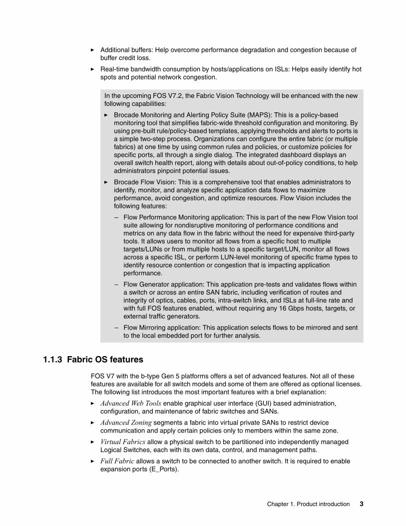
� Additional buffers: Help overcome performance degradation and congestion because of buffer credit loss.
� Real-time bandwidth consumption by hosts/applications on ISLs: Helps easily identify hot spots and potential network congestion.
1.1.3 Fabric OS features
FOS V7 with the b-type Gen 5 platforms offers a set of advanced features. Not all of these features are available for all switch models and some of them are offered as optional licenses. The following list introduces the most important features with a brief explanation:
� Advanced Web Tools enable graphical user interface (GUI) based administration, configuration, and maintenance of fabric switches and SANs.
� Advanced Zoning segments a fabric into virtual private SANs to restrict device communication and apply certain policies only to members within the same zone.
� Virtual Fabrics allow a physical switch to be partitioned into independently managed Logical Switches, each with its own data, control, and management paths.
� Full Fabric allows a switch to be connected to another switch. It is required to enable expansion ports (E_Ports).
In the upcoming FOS V7.2, the Fabric Vision Technology will be enhanced with the new following capabilities:
� Brocade Monitoring and Alerting Policy Suite (MAPS): This is a policy-based monitoring tool that simplifies fabric-wide threshold configuration and monitoring. By using pre-built rule/policy-based templates, applying thresholds and alerts to ports is a simple two-step process. Organizations can configure the entire fabric (or multiple fabrics) at one time by using common rules and policies, or customize policies for specific ports, all through a single dialog. The integrated dashboard displays an overall switch health report, along with details about out-of-policy conditions, to help administrators pinpoint potential issues.
� Brocade Flow Vision: This is a comprehensive tool that enables administrators to identify, monitor, and analyze specific application data flows to maximize performance, avoid congestion, and optimize resources. Flow Vision includes the following features:
– Flow Performance Monitoring application: This is part of the new Flow Vision tool suite allowing for nondisruptive monitoring of performance conditions and metrics on any data flow in the fabric without the need for expensive third-party tools. It allows users to monitor all flows from a specific host to multiple targets/LUNs or from multiple hosts to a specific target/LUN, monitor all flows across a specific ISL, or perform LUN-level monitoring of specific frame types to identify resource contention or congestion that is impacting application performance.
– Flow Generator application: This application pre-tests and validates flows within a switch or across an entire SAN fabric, including verification of routes and integrity of optics, cables, ports, intra-switch links, and ISLs at full-line rate and with full FOS features enabled, without requiring any 16 Gbps hosts, targets, or external traffic generators.
– Flow Mirroring application: This application selects flows to be mirrored and sent to the local embedded port for further analysis.
Chapter 1. Product introduction 3

� The Adaptive Networking service is a set of features that provides users with tools and capabilities for incorporating network policies to ensure optimal behavior in a large SAN. FOS V7.0 supports two types of quality of service (QoS) features with the 16 Gbps fabric backbones: ingress rate limiting and session ID (SID)/DID-based prioritization.
� Server Application Optimization (SAO) enhances overall performance and virtual machine scalability by extending b-type data center fabric technologies to the server infra-structure. SAO enables individual traffic flows to be configured, prioritized, and optimized, from end to end, throughout the data center.
� Enhanced Group Management (EGM) enables additional device-level management functions for IBM b-type SAN products when it is added to the element management. It also allows large consolidated operations, such as firmware downloads and configuration uploads and downloads for groups of devices.
� Extended Fabrics extend SAN fabrics beyond the Fibre Channel standard of 10 km by optimizing internal switch buffers to maintain performance on ISLs that are connected at extended distances.
� Integrated Routing allows any 16 Gbps Fibre Channel port to be configured as an EX_Port supporting Fibre Channel Routing.
� Integrated 10 Gbps Fibre Channel Activation enables Fibre Channel ports to operate at 10 Gbps.
� Fabric Watch constantly monitors mission-critical switch operations for potential faults and automatically alerts administrators to problems before they become costly failures. Fabric Watch includes port fencing capabilities.
� FICON with Control Unit Port (CUP) Activation is designed to provide in-band management of the supported SAN b-type switch and director products by system automation for IBM z/OS® from IBM System z10® Enterprise Class and Business Class, IBM System z9® Enterprise Class and Business Class, IBM zSeries 990 and 890, and IBM zEnterprise® 196 and 114 servers. This support provides a single point of control for managing connectivity in active FICON I/O configurations. To enable in-band management on multiple switches and directors, each chassis must be configured with the appropriate FICON CUP feature. System automation for IBM OS/390® or z/OS can now use FICON to concurrently manage IBM ESCON® Director 3092, in addition to supported SAN b-type switch and director products.
� An Inter-chassis license with 16× (4×16 Gbps) QSFP provides connectivity up to 100 meters from the switching backplane of one half of an eight-slot chassis to the other half, or to a 4-slot chassis.
� An Enterprise ICL license supports up to 3,840 16 Gbps universal Fibre Channel ports (using 16 Gbps 48-port blades), up to 5,120 8 Gbps universal Fibre Channel ports (using 8 Gbps 64-port blades), and ICL ports (32 or 16 per chassis, with optical QSFP) connected up to nine chassis in a full-mesh topology or up to 10 chassis in a core-edge topology. Connecting five or more chassis through ICLs requires an Enterprise ICL license.
� An Advanced Extension activation license enables two advanced extension features, FCIP trunking and adaptive rate limiting (ARL), on the IBM System Networking SAN768B-2 or IBM System Networking SAN384B-2 systems. The FCIP trunking feature allows multiple IP source and destination address pairs (defined as FCIP circuits) through multiple 1 GbE interfaces to provide a high-bandwidth FCIP tunnel and failover resiliency. The ARL feature is designed to provide a minimum bandwidth guarantee for each tunnel with full usage of the available network bandwidth without impacting throughput performance under a high traffic load.
4 IBM b-type Gen 5 16 Gbps Switches and Network Advisor
� An Extension blade 10 GbE activation license enables up to two 10 GbE ports on the 8 Gbps extension blades or eight 10 Gbps Fibre Channel ports on the first eight ports of a 16 Gbps port blade. With this license, two additional operating modes, in addition to a 1 GbE port mode, can be selected. Either two 10 GbE ports, or ten 1 GbE and one 10 GbE ports, can be configured on an 8 Gbps extension blade when this license is activated.
� An FICON Accelerator activation license uses advanced networking technologies, data management techniques, and protocol intelligence to accelerate FICON disk and tape read-and-write operations over geographically extended distances, while also maintaining the integrity of command and acknowledgment sequences. Ideal for data migration, disaster recovery, and business continuity solutions beyond 300 km, it supports emulation for IBM z/OS Global Mirror (formerly Extended Remote Copy (XRC)) and tape pipelining for FICON tape and virtual tape.
� An Encryption 96 Gbps disk performance upgrade activation license enables scalability of performance on the encryption blade features. The upgrade is designed to provide increased throughput for disk encryption applications up to 96 Gbps, effectively doubling encrypted throughput performance for disk-based storage with no disruption to operations.
� Advanced Performance Monitoring helps identify end-to-end bandwidth usage by host/target pairs and is designed to provide for capacity planning.
� ISL Trunking enables Fibre Channel packets to be distributed efficiently across multiple ISLs between two IBM b-type SAN fabric switches and directors while preserving in-order delivery. Both b-type SAN devices must have trunking activated.
� Monitoring and Alerting Policy Suite (MAPS) is an optional storage area network (SAN) health monitor that allows you to enable each switch to constantly monitor its SAN fabric for potential faults and automatically alerts you to problems long before they become costly failures. MAPS cannot coexist with Fabric Watch.
� Flow Vision is a comprehensive tool that enables administrators to identify, monitor, and analyze specific application data flows to maximize performance, avoid congestion, and optimize resources.
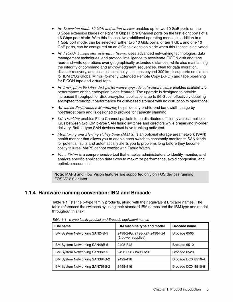
1.1.4 Hardware naming convention: IBM and Brocade
Table 1-1 lists the b-type family products, along with their equivalent Brocade names. The table references the switches by using their standard IBM names and the IBM type and model throughout this text.
Table 1-1 b-type family product and Brocade equivalent names
Note: MAPS and Flow Vision features are supported only on FOS devices running FOS V7.2.0 or later.
IBM name IBM machine type and model Brocade name
IBM System Networking SAN24B-5 2498-24G, 2498-X24 2498-F24 (2 power supplies)
Brocade 6505
IBM System Networking SAN48B-5 2498-F48 Brocade 6510
IBM System Networking SAN96B-5 2498-F96 / 2498-N96 Brocade 6520
IBM System Networking SAN384B-2 2499-416 Brocade DCX 8510-4
IBM System Networking SAN768B-2 2499-816 Brocade DCX 8510-8
Chapter 1. Product introduction 5

1.1.5 Fabric Operating System hardware support
FOS V7.x supports only 8 Gbps and 16 Gbps hardware platforms. To get the latest list of supported devices, read the IBM SAN b-type Firmware Version 7.x Release Notes, which are available at the following website:
http://www-01.ibm.com/support/docview.wss?uid=ssg1S1003855
1.1.6 Management
The b-type Gen 5 Fibre Channel directors and switches can be managed in several ways:
� IBM Network Advisor is a software management platform that unifies network management for SAN and converged networks. It provides users with a consistent user interface, proactive performance analysis, and troubleshooting capabilities across Fibre Channel (FC) and b-type FCoE installations.
� Web Tools is a built-in web-based application that provides administration and management functions on a per switch basis.
� A command-line interface (CLI) enables an administrator to monitor and manage individual switches, ports, and entire fabrics from a standard workstation. It accessed through Telnet, SSH, or serial console.
� SMI Agent enables integration with SMI-compliant Storage Resource Management (SRM) solutions, such as IBM Tivoli® Storage Productivity Center. The SMI Agent is embedded in the IBM Network Advisor.
Because the IBM Network Advisor is the preferred tool to manage the b-type Gen 5 fabrics, Chapter 3, “IBM Network Advisor” on page 65 provides detailed information bout how to install and configure IBM Network Advisor.
1.1.7 Monitoring
There are several monitor tools and notification methods that allow you to monitor your entire b-type Gen 5 fabric and even integrate with external applications.
Health monitorsFabric Watch and MAPS are monitors that allow you to enable each switch to constantly monitor its SAN fabric for potential faults and automatically alerts you to problems long before they become costly failures. MAPS is available only in FOS V7.2.0 or later.
Performance monitorsAdvanced Performance Monitoring and Flow Vision are performance monitors that integrate with IBM network Advisor. Flow Vision is available only in FOS V7.2.0 or later.
Notification methodsThere are several alert mechanisms that can be used, such as email messages, SNMP traps, and log entries. Fabric Watch allows you to configure multiple email recipients.
Note: Data Center Fabric Manager (DCFM) is not qualified with and does not support the management of switches operating with FOS V7.0 and later firmware versions. You must first upgrade DCFM to Network Advisor V12.0 if you are planning to upgrade devices to FOS V7.1.0 or later.
6 IBM b-type Gen 5 16 Gbps Switches and Network Advisor

An email alert sends information about a switch event to a one or multiple specified email addresses.
The Simple Network Management Protocol (SNMP) notification method is an efficient way to avoid having to log in to each switch individually, which you must do for error log notifications.
The RASLog (switch event log) can be forward to a central station. IBM Network Advisor can be configured as a syslog recipient for the SAN devices.
1.1.8 IBM Network Advisor
IBM Network advisor is the preferred tool for managing and monitoring the IBM b-type Gen 5 SANs. It is a software management tool that provides comprehensive management for data, storage, and converged networks.
It includes an intuitive interface, and provides an in-depth view of performance measures and historical data. It receives SNMP traps, syslog event messages, and customizable event alerts, and contains the Advanced Call Home feature that enables you to automatically collect diagnostic information and send notifications to IBM Support for faster fault diagnosis and isolation.
For more information about installing and configure IBM Network Advisor, see Chapter 3, “IBM Network Advisor” on page 65.
1.2 Product descriptions
This section provides a brief description of each b-type Gen 5 SAN switch or backbone.
1.2.1 IBM System Networking SAN24B-5
The SAN24B-5 is an entry level SAN switch that combines flexibility, simplicity, and enterprise-class functions. It is a 1U form factor unit configurable in 12 or 24 ports and supports 2, 4, 8 or 16 Gbps speeds. It can be deployed as a full-fabric switch or as an (NPIV enabled) Access Gateway enabling the creation of dense fabrics in a relatively small space. It includes one or two power supplies based upon the model (2498-24G/2498-X24 or 2498-F24).
Figure 1-1 shows the IBM System Networking SAN24B-5 fabric switch.
Figure 1-1 SAN24B-5 switch
Chapter 1. Product introduction 7
The SAN24B-5 requires FOS V7.0.1 or later. The Advanced Web Tools, Advanced Zoning, Full Fabric, and Enhanced Group Management features are part of the base Fabric OS and do not require a license. Additional features, such as Adaptive networking, Advanced Performance Monitor, Fabric Watch, Inter-Switch Link (ISL) Trunking, Extended Fabrics, Server Application Optimization, and 12-port Activation are available as optional licenses. Furthermore, an Enterprise Package is available as a bundle that includes one license for each of the optional licenses, except the Extended Fabrics one. IBM Network Advisor V11.1 (or later) is the base management software for the SAN24B-5, which can provide end-to-end data center fabric management.
Platform featuresHere are some of the features of the SAN24B-5:
� Up to 24 auto-sensing ports of high-performance 16-Gbps technology in a single domain.
� Ports on Demand scaling (12 - 24 ports).
� 2, 4, 8, and 16 Gbps auto-sensing Fibre Channel switch and router ports.
– 2, 4, and 8 Gbps performance is enabled by 8 Gbps SFP+ transceivers.
– 4, 8, and 16 Gbps performance is enabled by 16 Gbps SFP+ transceivers.
� Universal ports self-configure as E, F, or M ports. EX_Ports can be activated on a per-port basis with the optional Integrated Routing license. The D-port function is also available for diagnostic tests.
� Airflow is set for port side exhaust.
� Inter-Switch Link (ISL) Trunking, which allows up to eight ports (at 2, 4, 8, or 16 Gbps speeds) between a pair of switches to combine to form a single, logical ISL with a speed of up to 128 Gbps (256 Gbps full duplex) for optimal bandwidth usage and load balancing. The base model permits one eight-port trunk plus one four-port trunk.
� Dynamic Path Selection (DPS), which optimizes fabric-wide performance and load balancing by automatically routing data to the most efficient available path in the fabric.
� Brocade-branded SFP+ optical transceivers that support any combination of Short Wavelength (SWL), Long Wavelength (LWL), and Extended Long Wavelength (ELWL) optical media among the switch ports
� Extended distance support enables native Fibre Channel extension up to 7,500 km at 2 Gbps.
� Support for unicast traffic type.
� FOS, which delivers distributed intelligence throughout the network and enables a wide range of added value applications, including Brocade Advanced Web Tools, Brocade Enhanced Group Management, and Brocade Zoning.
� Support for Access Gateway configuration where server ports connected to the fabric core are virtualized.
� Hardware zoning is accomplished at the port level of the switch and by worldwide name (WWN). Hardware zoning permits or denies delivery of frames to any destination port address.
� Extensive diagnostic and system-monitoring capabilities for enhanced high reliability, availability, and serviceability (RAS).
� The Brocade EZSwitchSetup wizard makes SAN configuration a three-step point-and-click task.
� Real-time power monitoring enables users to monitor real-time power usage of the fabric at a switch level.
8 IBM b-type Gen 5 16 Gbps Switches and Network Advisor

1.2.2 IBM System Networking SAN48B-5
The SAN48B-5 is a flexible, easy-to-use Enterprise-Class SAN switch for private cloud storage. It is a 1U form factor unit that is configurable in 24, 36 or 48 ports and supports auto-sensing 2, 4, 8, or 16 Gbps and 10 Gbps speeds. It can be deployed as a full-fabric switch or as an (NPIV enabled) Access Gateway. It is also enhanced with enterprise connectivity that adds support for IBM FICON. It includes dual, hot-swappable redundant power supplies with integrated system cooling fans.
Figure 1-2 shows the IBM System Networking SAN48B-5 fabric switch.
Figure 1-2 SAN48B-5 switch
The SAN48B-5 requires FOS V7.0 or later. The Advanced Web Tools, Advanced Zoning, Enhanced Group Management, Fabric Watch, Full Fabric, and Virtual Fabrics features are included in the base FOS and do not require an additional license. Additional features such as twelve-port Activation, FICON with CUP Activation, Adaptive Networking, Advanced Performance Monitoring, Extended Fabrics, Integrated Routing, ISL Trunking, Server Application Optimization (SAO), and Integrated 10 Gbps Fibre Channel Activation are available as optional licenses. The Enterprise Advanced Bundle includes one license for each of the Extended Fabric, Advanced Performance Monitoring, Trunking Activation, Adaptive Networking, and SAO functions. IBM Network Advisor V11.1 (or later) is the base management software for the SAN48B-5.
Platform featuresHere are some of the features of the SAN48B-5:
� Up to 48 auto-sensing ports of high-performance 16 Gbps technology in a single domain.
� Ports on Demand scaling (24 - 36 or 48 ports).
� 2, 4, 8, and 16 Gbps auto-sensing Fibre Channel switch and router ports.
– 2, 4, and 8 Gbps performance is enabled by 8 Gbps SFP+ transceivers.
– 4, 8, and 16 Gbps performance is enabled by 16 Gbps SFP+ transceivers.
� 10 Gbps manual set capability on FC ports (requires the optional 10 Gigabit FCIP/Fibre Channel license).
� 10 Gbps performance is enabled by 10 Gbps SFP+ transceivers.
� Ports can be configured for 10 Gbps for metro connectivity (on the first eight ports only).
� Universal ports self-configure as E, F, M, or D ports. EX_Ports can be activated on a per port basis with the optional Integrated Routing license.
� The Brocade Diagnostic Port (D-Port) feature provides physical media diagnostic, troubleshooting, and verification services.
� In-flight data compression and encryption on up to two ports provides efficient link usage and security.
� Options for port side exhaust (default) or nonport side exhaust airflow for cooling.
Chapter 1. Product introduction 9

� Virtual Fabric support to improve isolation between different VFs.
� Fibre Channel Routing (FCR) service, which is available with the optional Integrated Routing license, provides improved scalability and fault isolation.
� FICON, FICON Cascading, and FICON Control Unit Port ready.
� Inter-Switch Link (ISL) Trunking (licensable), which allows up to eight ports (at 2, 4, 8, or 16 Gbps speeds) between a pair of switches to combine to form a single, logical ISL with a speed of up to 128 Gbps (256 Gbps full duplex) for optimal bandwidth usage and load balancing.
� Dynamic Path Selection (DPS), which optimizes fabric-wide performance and load balancing by automatically routing data to the most efficient available path in the fabric.
� Brocade-branded SFP+ optical transceivers that support any combination of Short Wavelength (SWL), Long Wavelength (LWL), or Extended Long Wavelength (ELWL) optical media among the switch ports.
� Extended distance support enables native Fibre Channel extension up to 7,500 km at 2 Gbps.
� Support for unicast, multicast (255 groups), and broadcast data traffic types.
� FOS, which delivers distributed intelligence throughout the network and enables a wide range of added value applications, including Brocade Advanced Web Tools and Brocade Zoning. Optional Fabric Services include Adaptive Networking with QoS, Brocade Extended Fabrics, Brocade Enhanced Group Management, Brocade Fabric Watch, ISL Trunking, and End-to-End Performance Monitoring (APM).
� Support for Access Gateway configuration where server ports are connected to the fabric core is virtualized.
� Hardware zoning is accomplished at the port level of the switch and by a worldwide name (WWN). Hardware zoning permits or denies delivery of frames to any destination port address.
� Extensive diagnostic and system-monitoring capabilities for enhanced high reliability, availability, and serviceability (RAS).
� 10G Fibre Channel integration on the same port provides for DWDM metro connectivity on the same switch (can be done on first eight ports only).
� The Brocade EZSwitchSetup wizard makes SAN configuration a three-step point-and-click task.
� Real-time power monitoring enables users to monitor real-time power usage of the fabric at a switch level.
1.2.3 IBM System Networking SAN96B-5
The SAN96B-5 is a scalable Enterprise-Class SAN Switch for highly virtualized cloud environments. It is a 2U form factor unit configurable in 48, 72, or 96 ports and supports auto-sensing 2, 4, 8, or 16 Gbps and 10 Gbps speeds. This switch also features dual-direction airflow options to support the latest hot aisle/cold aisle configurations (2498-F96 and 2498-N96). It does not support the Access Gateway function or IBM FICON connectivity.
Figure 1-3 on page 11 shows the IBM System Networking SAN96B-5 fabric switch.
10 IBM b-type Gen 5 16 Gbps Switches and Network Advisor

Figure 1-3 AN96B-5 switch
The SAN968B-5 requires FOS V7.1 or later. The Advanced Web Tools, Advanced Zoning, Virtual Fabrics, Full Fabric, Adaptive Networking, Server Application Optimization, and Enhanced Group Management features are included in the base FOS and do not require an additional license. Additional features such as 24-port Activation, Advanced Performance Monitor, Fabric Watch, Extended Fabrics, Integrated Routing, Trunking Activation, Integrated 10 Gbps Fibre Channel Activation are available as optional licenses. The optional Enterprise Advanced Bundle includes one license for each of the Fabric Watch, Extended Fabric, Advanced Performance Monitor, and Trunking Activation features. IBM Network Advisor V12.0 (or later) is the base management software for the SAN96B-5.
Platform featuresHere are some of the SAN96B-5 features:
� Up to 96 auto-sensing ports of high-performance 16 Gbps technology in a single domain.
� Ports on Demand scaling (48 - 72 or 96 ports).
� Port licensing through DPOD
� 2, 4, 8, and 16 Gbps auto-sensing Fibre Channel switch and router ports.
– 2, 4, and 8 Gbps performance is enabled by 8 Gbps SFP+ transceivers.
– 4, 8, and 16 Gbps performance is enabled by 16 Gbps SFP+ transceivers.
� 10 Gbps manual set capability on FC ports (requires the optional 10 Gigabit FCIP/Fibre Channel license) on the first eight ports only.
– Ports can be configured for 10 Gbps for metro connectivity.
– 10 Gbps performance is enabled by 10 Gbps Fibre Channel SFP+ transceivers.
� FC ports self-configure as E_ports and F_ports. EX_ports can be activated on a per-port basis with the optional Integrated Routing license.
� Mirror ports (M_ports) and diagnostic ports (D_ports) must be manually configured.
� The Brocade Diagnostic Port (D_port) feature provides physical media diagnostic, troubleshooting, and verification services.
� In-flight data compression and encryption on up to 16 ports (up to 8 ports at 16 Gbps) provides efficient link usage and security.
� Options for port side exhaust (default) or non-port side exhaust airflow for cooling.
� Virtual Fabric (VF) supports to improve isolation between different VFs.
� A Fibre Channel Routing (FCR) service, available with the optional Integrated Routing license, provides improved scalability and fault isolation.
Chapter 1. Product introduction 11

� Inter-Switch Link (ISL) Trunking (licensable), which allows up to eight ports (at 2, 4, 8, or 16 Gbps speeds) between a pair of switches to combine to form a single, logical ISL with a speed of up to 128 Gbps (256 Gbps full duplex) for optimal bandwidth usage and load balancing. There is no limit to how many trunk groups can be configured.
� Dynamic Path Selection (DPS), which optimizes fabric-wide performance and load balancing by automatically routing data to the most efficient available path in the fabric.
� Brocade-branded SFP+ optical transceivers that support any combination of Short Wavelength (SWL), Long Wavelength (LWL), or Extended Long Wavelength (ELWL) optical media among the switch ports.
� Extended distance support enables native Fibre Channel extension up to 7,500 km at 2 Gbps.
� Support for unicast data traffic types.
� FOS, which delivers distributed intelligence throughout the network and enables a wide range of added value applications, including Brocade Advanced Web Tools and Brocade Zoning. Optional Fabric Services include Adaptive Networking with QoS, Brocade Extended Fabrics, Brocade Enhanced Group Management, Brocade Fabric Watch, ISL Trunking, and End-to-End Advanced Performance Monitoring (APM).
� Hardware zoning is accomplished at the port level of the switch and by worldwide name (WWN). Hardware zoning permits or denies delivery of frames to any destination port address.
� Extensive diagnostic and system-monitoring capabilities for enhanced high reliability, availability, and serviceability (RAS).
� 10 Gbps Fibre Channel integration on the same port provides for DWDM metro connectivity on the same switch (can be done on first eight ports only with appropriate licensing).
� The Brocade EZSwitchSetup wizard makes SAN configuration a three-step point-and-click task.
� Real-time power monitoring enables users to monitor real-time power usage of the fabric at a switch level
1.2.4 IBM System Networking SAN384B-2 and IBM System Networking SAN768B-2
The SAN384B-2 and SAN768B-2 backbones deliver a new level of scalability and advanced capabilities to this robust, reliable, and high-performance technology. These capabilities enable organizations to continue using their existing IT investments as they grow their businesses. In addition, these businesses can consolidate their storage area network (SAN) infrastructures to simplify management and reduce operating costs. The UltraScale ICL technology that is available in these backbones includes new optical ports, higher port density, and support for standard optical cables up to 100 meters. The UltraScale ICLs can connect up to 10 Brocade DCX 8510 Backbones, enabling flatter, faster, and simpler fabrics that increase consolidation while reducing network complexity and costs.
12 IBM b-type Gen 5 16 Gbps Switches and Network Advisor
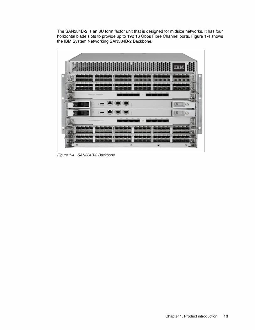
The SAN384B-2 is an 8U form factor unit that is designed for midsize networks. It has four horizontal blade slots to provide up to 192 16 Gbps Fibre Channel ports. Figure 1-4 shows the IBM System Networking SAN384B-2 Backbone.
Figure 1-4 SAN384B-2 Backbone
Chapter 1. Product introduction 13
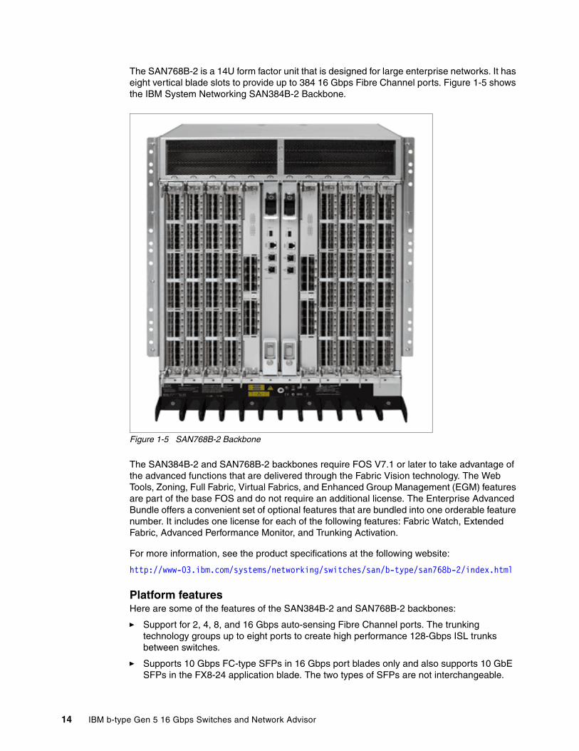
The SAN768B-2 is a 14U form factor unit that is designed for large enterprise networks. It has eight vertical blade slots to provide up to 384 16 Gbps Fibre Channel ports. Figure 1-5 shows the IBM System Networking SAN384B-2 Backbone.
Figure 1-5 SAN768B-2 Backbone
The SAN384B-2 and SAN768B-2 backbones require FOS V7.1 or later to take advantage of the advanced functions that are delivered through the Fabric Vision technology. The Web Tools, Zoning, Full Fabric, Virtual Fabrics, and Enhanced Group Management (EGM) features are part of the base FOS and do not require an additional license. The Enterprise Advanced Bundle offers a convenient set of optional features that are bundled into one orderable feature number. It includes one license for each of the following features: Fabric Watch, Extended Fabric, Advanced Performance Monitor, and Trunking Activation.
For more information, see the product specifications at the following website:
http://www-03.ibm.com/systems/networking/switches/san/b-type/san768b-2/index.html
Platform featuresHere are some of the features of the SAN384B-2 and SAN768B-2 backbones:
� Support for 2, 4, 8, and 16 Gbps auto-sensing Fibre Channel ports. The trunking technology groups up to eight ports to create high performance 128-Gbps ISL trunks between switches.
� Supports 10 Gbps FC-type SFPs in 16 Gbps port blades only and also supports 10 GbE SFPs in the FX8-24 application blade. The two types of SFPs are not interchangeable.
14 IBM b-type Gen 5 16 Gbps Switches and Network Advisor

� The 10 Gbps ports can be configured manually on only the first eight ports of the 16 Gbps port blades.
� Beginning with FOS V7.0.1, up to nine chassis in a full mesh (or ten in a core-edge) topology can be connected by using 4x 16 Gbps quad SFP (QSFP) inter-chassis links (ICLs). FOS V7.0.0 permits up to six chassis to be linked.
� Support for high-performance port blades running at 2, 4, 8, 10, or 16 Gbps, enabling flexible system configuration.
� Redundant and hot-swappable control processor and core switch blades, power supplies, blower assemblies, and WWN cards that enable a high availability platform and enable nondisruptive software upgrades for mission-critical SAN applications.
� Universal ports that self-configure as E_Ports, F_Ports, EX_Ports, and M_Ports (mirror ports). 10 Gbps ports are E_Ports only.
� Diagnostic port (D_Port) function.
� In-flight data cryptographic (encryption/decryption) and data compression capabilities through the 16 Gbps port blades.
� Fibre Channel over IP (FCIP) function through the FX8-24 blade.
For more information about the b-type Gen 5 products, see Chapter 2, “Product hardware and features” on page 17.
Chapter 1. Product introduction 15

16 IBM b-type Gen 5 16 Gbps Switches and Network Advisor

Chapter 2. Product hardware and features
This chapter introduces the new IBM b-type Gen 5 16 Gbps SAN switches and their new hardware features, including the Gen 5 hardware enhancements and the Fabric Vision features and technology.
This chapter provides a high-level guideline about the most commonly encountered SAN topologies.
2
© Copyright IBM Corp. 2014. All rights reserved. 17

2.1 Topologies
Before introducing the features of the hardware and software, this chapter provides a brief overview of the topologies that are commonly encountered.
A topology is described in terms of how the switches are interconnected, such as ring, core-edge, and edge-core-edge or fully meshed.
The preferred SAN topology to optimize performance, management, and scalability is a tiered, core-edge topology (sometimes called core-edge or tiered core edge). This approach provides good performance without unnecessary interconnections. At a high level, the tiered topology has many edge switches that are used for device connectivity, and fewer core switches that are used for routing traffic between the edge switches, as shown in Figure 2-1.
Figure 2-1 Four scenarios of tiered network topologies (hops shown in heavier, orange connections)
� Scenario A has localized traffic, which can have small performance advantages but does not provide ease of scalability or manageability.
� Scenario B, also known as edge-core, separates the storage and servers, thus providing ease of management and moderate scalability.
� Scenario C, also known as edge-core-edge, has both storage and servers on edge switches, which provide ease of management and is much more scalable.
� Scenario D is a full-mesh topology, and server to storage is no more than one hop. Designing with UltraScale ICLs is an efficient way to save front-end ports, and users can easily build a large (for example, 1536-port or larger) fabric with minimal SAN design considerations.
2.1.1 Edge-core topology
The edge-core topology (Scenario B in Figure 2-1) places initiators (servers) on the edge tier and storage (targets) on the core tier. Because the servers and storage are on different switches, this topology provides ease of management and good performance, with most traffic traversing only one hop from the edge to the core.
The disadvantage to this design is that the storage and core connections are in contention for expansion.
Note: Adding an IBM SAN director as the SAN core can reduce the expansion contention.
18 IBM b-type Gen 5 16 Gbps Switches and Network Advisor

2.1.2 Edge-core-edge topology
The edge-core-edge topology (Scenario C in Figure 2-1 on page 18) places initiators on one edge tier and storage on another edge tier, leaving the core for switch interconnections or connecting devices with network-wide scope, such as Dense Wavelength Division Multiplexers (DWDMs), inter-fabric routers, storage virtualizers, tape libraries, and encryption engines.
Because servers and storage are on different switches, this design enables independent scaling of compute and storage resources, ease of management, and optimal performance, with traffic traversing only two hops from the edge through the core to the other edge. In addition, it provides an easy path for expansion because ports and switches can readily be added to the appropriate tier as needed.
2.1.3 Full-mesh topology
A full-mesh topology (Scenario D in Figure 2-1 on page 18) allows you to place servers and storage anywhere because the communication between source to destination is no more than one hop. With optical UltraScale ICLs, you can build a full-mesh topology that is scalable and cost-effective compared to the previous generation of SAN products.
2.2 Gen 5 Fibre Channel technology
Gen 5 is the latest SAN technology that is designed to provide 16 Gbps performance for supporting emerging work loads, the growing virtualized environment, and low latency SSD and flash-based storage generation.
This section cover the new Gen 5 Fibre Channel technology and its features, and the Gen 5 hardware.
2.2.1 Condor3 ASIC
The Condor3 ASIC is the kernel of the Gen 5 switches. Condor3 ASIC provides unmatched performance compared to its predecessors. Condor3 ASIC increases the frames that are switched per second and the total throughput bandwidth combined with increased energy efficiency. Here are some of the significant Condor3 ASIC specifications:
� Performance and compatibility:
– 420 million frames that are switched per second
– 768 Gbps of bandwidth
– 16/10/8/4/2 Gbps speed
– EX/E/F/M/“D” on any port
� Industry-leading efficiency with less than 1 watt/Gbps.
� More scalable across distance:
– 8000 buffers (four times of what exists on Gen 4)
– Up to 5000 km distance at 2 Gbps
Note: Hop count is not a concern if the total switching latency is less than the disk I/O timeout value.
Chapter 2. Product hardware and features 19

� Unmatched investment protection that is compatible with over 30 million existing SAN ports.
� UltraScale Optical ICLs support optical connections to up 10 chassis and distances up to 100 meters.
� Fabric Vision provides advanced diagnostic tests, monitoring, and management that maximizes availability, resiliency, and performance.
� ClearLink Diagnostic Ports ensure link-level integrity from the server adapter across fabrics and ICLs.
� Forward Error Correction. Automatic recovery of transmission errors enhances reliability of transmission, which in turn results in higher availability and performance.
� In-flight Encryption/Compression.
� Secure ISL connectivity and compression of ISL traffic for bandwidth optimization.
� Using 10 Gbps Native Fibre Channel, you can configure any Condor3 port because 10 Gbps Fibre Channel eliminates the need for specialized ports for optical MAN (10 Gbps DWDM) connectivity.
� ASIC-Enabled Buffer Credit loss Detection and Automatic Recovery at Virtual Channel Level.
� Auto Link Tuning for Back-end Ports.
� E_Port Top Talkers and Concurrency with Fibre Channel Routing.
� Monitors top bandwidth-consuming flows in real time on each individual ISL and EX_Ports.
2.2.2 Fabric Vision
Fabric Vision is partially compatible with Gen 4 switches and fully supported on Gen 5 switches, Fabric Vision is a set of new software features that works with the new Gen 5 hardware capabilities to provide advanced diagnostic tests, improved monitoring, and management. It is designed to maximize availability, resiliency, performance, and simplify SAN deployment and management.
There are many important technologies behind Fabric Vision:
� Switch, director, and adapter ASICs.
� Delivery in Brocade Fabric Operating System (FOS) begins primarily with Version 7.0, with some features available before then.
� Adapter driver beginning with Version 3.1.
� IBM Network Advisor V12.0 and later delivers important parts of the new architecture.
Here are the main Fabric Vision features:
� ClearLink Diagnostic Ports: Ensures optical and signal integrity for Gen 5 Fibre Channel optics and cables.
� Latency Bottleneck Detection: Enables proactive monitoring, alerting, and visualization of high latency devices and high latency ISLs that are impacting application performance. It simplifies SAN administration by narrowing troubleshooting efforts.
� Forward Error Correction (FEC): Automatically detects and recovers from bit errors, enhancing transmission reliability and performance.
20 IBM b-type Gen 5 16 Gbps Switches and Network Advisor

� Buffer Credit Recovery at the VC level: Automatically detects and recovers buffer credit loss at the Virtual Channel level, providing protection against performance degradation and enhancing application availability.
� Health and Performance Dashboards: Integration with IBM Network Advisor, providing all the critical information in one window.
� Monitoring and Alerting Policy Suite (MAPS): Policy-based monitoring tool that simplifies fabric-wide threshold configuration and monitoring.
� Flow Vision: A comprehensive tool that enables administrators to identify, monitor, and analyze specific application data flows without using taps.
ClearLink Diagnostic PortsClearLink Diagnostic Ports identify and isolate optics and cable problems faster by reducing fabric deployment and diagnostic times.
Here are its main functions:
� Non-intrusively verifies transceiver and cable health
� Tests electrical and optical transceiver components
� Monitors and trends transceiver health based on uptime
� Conducts cable health checks
� Monitors and sets alerts for digital diagnostic tests
� Ensures predictable application performance over links
� Provides granular latency and distance measurement for buffer credit assignment
� Simulates application-level I/O profiles
The background that ensures the advanced diagnostic tests for 16G SFP+ and 16G links is a new diagnostic port type that is known as D_Port. D_Port is used to diagnose optics and cables and it is configured by the user to run diagnostic tests.
D_Port mode allows you to convert a Fibre Channel port into a diagnostic port for testing link traffic, electrical loopbacks, and optical loopbacks between a pair of switches, a pair of access gateways, and a switch. Support is also provided for running D_Port tests between a host bus adapter (HBA) and a switch. The test results that are reported can be useful in diagnosing various port and link problems.
Understanding D_PortD_Port does not carry any user traffic and is designed to run only specific diagnostic tests for identifying link-level faults or failures. Basically, to start a port in D_Port mode, you must configure both ends of the link between a pair of switches (or switches configured as Access Gateways), and you must disable the existing port before you can configure it as a D_Port.
Note: MAPS and Flow Vision are available only with FOS V7.2 or later.
Note: D_Port ports must use 10G or 16G Brocade-branded SFPs.
Chapter 2. Product hardware and features 21
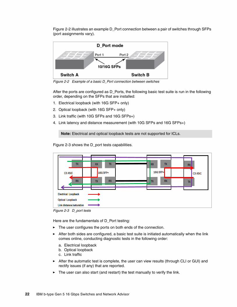
Figure 2-2 illustrates an example D_Port connection between a pair of switches through SFPs (port assignments vary).
Figure 2-2 Example of a basic D_Port connection between switches
After the ports are configured as D_Ports, the following basic test suite is run in the following order, depending on the SFPs that are installed:
1. Electrical loopback (with 16G SFP+ only)
2. Optical loopback (with 16G SFP+ only)
3. Link traffic (with 10G SFPs and 16G SFPs+)
4. Link latency and distance measurement (with 10G SFPs and 16G SFPs+)
Figure 2-3 shows the D_port tests capabilities.
Figure 2-3 D_port tests
Here are the fundamentals of D_Port testing:
� The user configures the ports on both ends of the connection.
� After both sides are configured, a basic test suite is initiated automatically when the link comes online, conducting diagnostic tests in the following order:
a. Electrical loopbackb. Optical loopbackc. Link traffic
� After the automatic test is complete, the user can view results (through CLI or GUI) and rectify issues (if any) that are reported.
� The user can also start (and restart) the test manually to verify the link.
Note: Electrical and optical loopback tests are not supported for ICLs.
22 IBM b-type Gen 5 16 Gbps Switches and Network Advisor

Advantages of ClearLink Diagnostic portsUse the D_Port tests for the following situations:
� Testing a new link before adding it to the fabric� Testing a trunk member before joining it with the trunk� Testing long-distance cables and SFPs
Tests can be run with the following options:
� Number of test frames to transmit� Size of test frames� Duration of the test� User-defined test payload� Predefined pattern for use in the test payload� Testing with forward error correction (FEC) on or off (default is off)� Testing with credit recovery (CR) on or off (default is off)
For more information, see 7.3, “Diagnostic features” on page 254.
Latency Bottleneck DetectionA bottleneck is a port in the fabric where frames cannot get through as fast as they should. A bottleneck is a port where the offered load is greater than the achieved egress throughput. Bottlenecks can cause unwanted degradation in throughput on various links. When a bottleneck occurs at one place, other points in the fabric can experience bottlenecks as the traffic backs up.
The Latency Bottleneck Detection feature enables you to do the following tasks:
� Prevent degradation of throughput in the fabric.
The bottleneck detection feature alerts you to the existence and locations of devices that are causing latency. If you receive alerts for one or more F_Ports, use the CLI to check whether these F_Ports have a history of bottlenecks.
� Reduce the time that it takes to troubleshoot network problems.
If you notice one or more applications that are slowing down, you can determine whether any latency devices are attached to the fabric and where. You can use the CLI to display a history of bottleneck conditions on a port. If the CLI shows above-threshold bottleneck severity, you can narrow the problem down to device latency rather than problems in the fabric.
A latency bottleneck is a port where the offered load exceeds the rate at which the other end of the link can continuously accept traffic, but does not exceed the physical capacity of the link. This condition can be caused by a device that is attached to the fabric that is slow to process received frames and send back credit returns. A latency bottleneck because of such a device can spread through the fabric and can slow down unrelated flows that share links with the slow flow.
As part of bottleneck detection, there is also the congestion bottleneck detection.
A congestion bottleneck is a port that is unable to transmit frames at the offered rate because the offered rate is greater than the physical data rate of the line. For example, this condition can be caused by trying to transfer data at 8 Gbps over a 4 Gbps ISL.
You can set alert thresholds for the severity and duration of the bottleneck. If a bottleneck is reported, you can then investigate and optimize the resource allocation for the fabric. Using the zone setup and Top Talkers, you can also determine which flows are destined to any affected F_Ports.
Chapter 2. Product hardware and features 23
You configure bottleneck detection on a per-fabric or per-switch basis, with per-port exclusions.
Supported configurations for bottleneck detectionNote the following configuration rules for bottleneck detection:
� The switch must be running FOS V6.4.0 or later.� Bottleneck detection is supported on Fibre Channel ports and FCoE F_Ports.� Bottleneck detection is supported on the following port types:
– E_Ports– EX_Ports– F_Ports– FL_Ports
� F_Port and E_Port trunks are supported.� Long-distance E_Ports are supported.� FCoE F_Ports are supported.� Bottleneck detection is supported on 4 Gbps, 8 Gbps, and 16 Gbps platforms.� Bottleneck detection is supported in Access Gateway mode.� Bottleneck detection is supported whether Virtual Fabrics is enabled or disabled. In VF
mode, bottleneck detection is supported on all fabrics, including the base fabric.
For more information about how bottlenecks are configured and displayed, see the Fabric OS Administrator’s Guide, which you can find at the following website:
http://my.brocade.com/
Forward Error CorrectionForward Error Correction (FEC) provides a data transmission error control method by including redundant data (error-correcting code) to ensure error-free transmission on a specified port or port range. When FEC is enabled, it can correct one burst of up to 11-bit errors in every 2112-bit transmission, whether the error is in a frame or a primitive. FEC is enabled by default, and is supported on E_Ports on 16 Gbps-capable switches and on the N_Ports and F_Ports of an access gateway using RDY, Normal (R_RDY), or Virtual Channel (VC_RDY) flow control modes. It enables automatically when negotiation with a switch detects FEC capability. This feature is enabled by default and persists after driver reloads and system reboots. It functions with features such as QoS, trunking, and BB_Credit recovery.
LimitationsHere are the limitations of this feature:
� FEC is configurable only on Gen 5 16 Gbps-capable switches.
� FEC is supported only on 1860 and 1867 Brocade Fabric Adapter ports operating in HBA mode that is connected to 16 Gbps Gen 5 switches running FOS V7.1 and later.
FEC is not supported in the following scenarios:
� When the HBA port speed changes to less than 16 Gbps, this feature is disabled.
� For HBA ports operating in loop mode or in direct-attach configurations.
� On ports with DWDM.
Note: Bottleneck detection is disabled by default. The preferred practice is to enable bottleneck detection on all switches in the fabric, and leave it on to gather statistics continuously.
24 IBM b-type Gen 5 16 Gbps Switches and Network Advisor
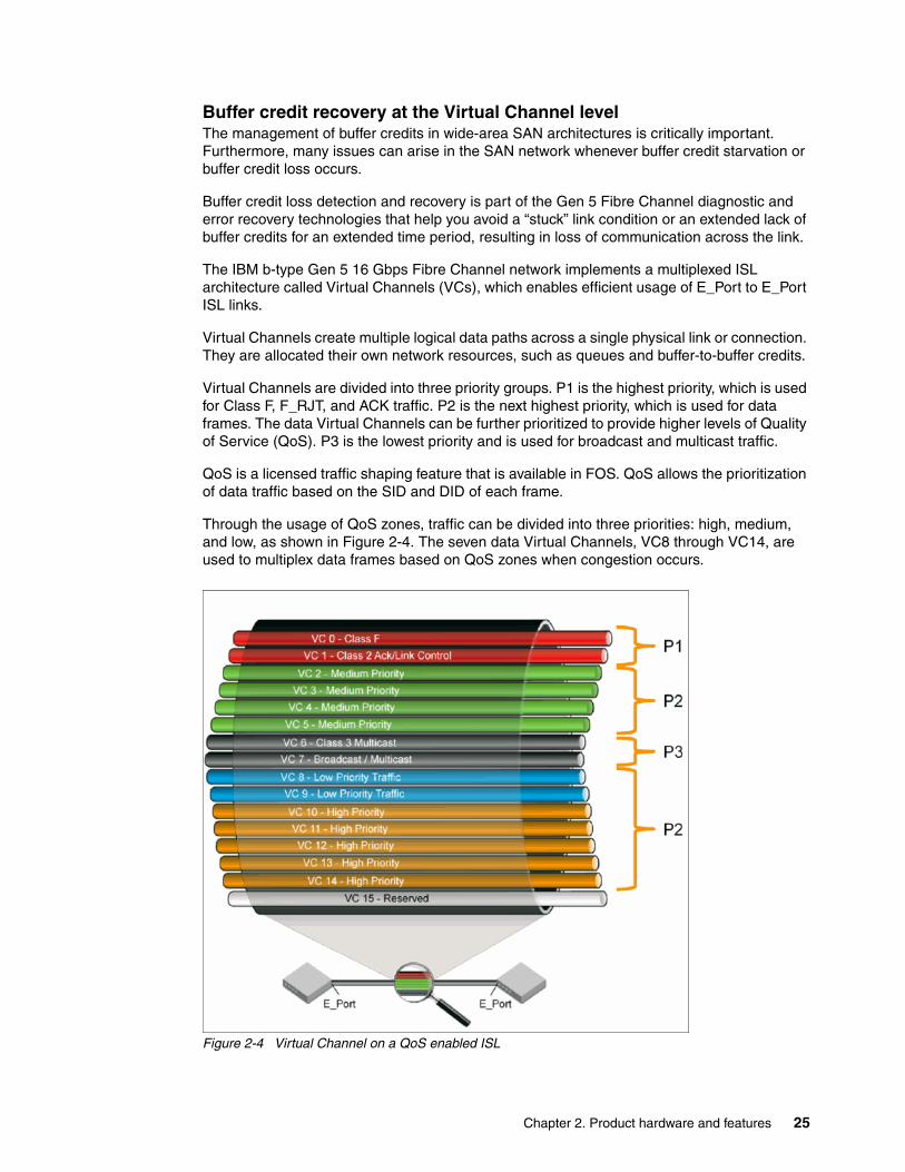
Buffer credit recovery at the Virtual Channel level The management of buffer credits in wide-area SAN architectures is critically important. Furthermore, many issues can arise in the SAN network whenever buffer credit starvation or buffer credit loss occurs.
Buffer credit loss detection and recovery is part of the Gen 5 Fibre Channel diagnostic and error recovery technologies that help you avoid a “stuck” link condition or an extended lack of buffer credits for an extended time period, resulting in loss of communication across the link.
The IBM b-type Gen 5 16 Gbps Fibre Channel network implements a multiplexed ISL architecture called Virtual Channels (VCs), which enables efficient usage of E_Port to E_Port ISL links.
Virtual Channels create multiple logical data paths across a single physical link or connection. They are allocated their own network resources, such as queues and buffer-to-buffer credits.
Virtual Channels are divided into three priority groups. P1 is the highest priority, which is used for Class F, F_RJT, and ACK traffic. P2 is the next highest priority, which is used for data frames. The data Virtual Channels can be further prioritized to provide higher levels of Quality of Service (QoS). P3 is the lowest priority and is used for broadcast and multicast traffic.
QoS is a licensed traffic shaping feature that is available in FOS. QoS allows the prioritization of data traffic based on the SID and DID of each frame.
Through the usage of QoS zones, traffic can be divided into three priorities: high, medium, and low, as shown in Figure 2-4. The seven data Virtual Channels, VC8 through VC14, are used to multiplex data frames based on QoS zones when congestion occurs.
Figure 2-4 Virtual Channel on a QoS enabled ISL
Chapter 2. Product hardware and features 25

IBM Gen 5 Fibre Channel switches can detect buffer credit loss at the VC level and, if the ASICs detect only a single buffer credit lost, can restore the buffer credit without interrupting the ISL data flow. If the ASICs detect more than one buffer credit lost or if they detect a “stuck” VC, they can recover from the condition by resetting the link, which requires retransmission of frames that were in transit across the link at the time of the link reset.
When a switch automatically detects and recovers buffer credit loss at the VC level, it provides protection against performance degradation and enhances application availability.
Health and Performance DashboardsThe IBM b-type Gen 5 16 Gbps switches, integrated with IBM Network Advisor V12.x and later, can provide all the critical information about the health and performance of a network in one window.
With a customizable dashboard, it is possible to define what is critical and what to monitor.
For more information, see 3.4, “New features of IBM Network Advisor V12.0.3” on page 116.
Monitoring and Alerting Policy SuiteThe Monitoring and Alerting Policy Suite (MAPS) is an optional storage area network (SAN) health monitor that supported on all switches running FOS V7.2.0 or later. It allows you to enable each switch to constantly monitor itself for potential faults and automatically alerts you to problems before they become costly failures.
MAPS tracks various SAN fabric metrics and events. Monitoring fabric-wide events, ports, and environmental parameters enables early fault detection and isolation and performance measurements.
MAPS provides a set of predefined monitoring policies that allow you to immediately use MAPS on activation.
In addition, MAPS provides customizable monitoring thresholds. These thresholds allow you to configure specific groups of ports or other elements so that they share a common threshold value. You can configure MAPS to provide notifications before problems arise, for example, when network traffic through a port is approaching the bandwidth limit. MAPS lets you define how often to check each switch and fabric measure and specify notification thresholds. Whenever fabric measures exceed these thresholds, MAPS automatically provides notification using several methods, including email messages, SNMP traps, and log entries.
The MAPS dashboard provides you with the ability to view quickly what is happening on the switch, and helps administrators dig deeper to see details about exactly what is happening on the switch (for example, the kinds of errors and the error count).
MAPS provides a seamless migration of all customized Fabric Watch thresholds, thus allowing you to take advantage of the advanced capabilities of MAPS. MAPS provides additional advanced monitoring, such as monitoring for the same error counters across different periods, or having more than two thresholds for any error counters. MAPS also provides support for you to monitor the statistics that are provided by the Flow Monitor feature of Flow Vision.
Note: MAPS cannot coexist with Fabric Watch.
26 IBM b-type Gen 5 16 Gbps Switches and Network Advisor

Flow VisionIntroduced in FOS V7.2, Flow Vision1 is a comprehensive tool that enables administrators to identify, monitor, and analyze specific application data flows.
Here are the Flow Vision features:
� Flow Monitor: Provides comprehensive visibility into application flows in the fabric, including the ability to learn (discover) flows automatically.
� Flow Mirror: You can use this function to nondisruptively create copies of the application flows, which can be captured for deeper analysis (only mirroring to processor is supported in FOS V7.2).
� Flow Generator: Test traffic generator for pre-testing the SAN infrastructure (including internal connections) for robustness before deploying the applications.
2.3 IBM System Networking SAN b-type family
This section provides an overview of the products and features in the IBM System Networking SAN b-type portfolio. For the latest information, see IBM System Networking SAN b-type website:
http://www.ibm.com/systems/networking/switches/san/b-type/index.html
Table 3-1 lists the Gen 4 and Gen 5 SAN switches and directors model number with speed and port capabilities, the current supported version of FOS, and the type of Application Specific Integrated Circuit (ASIC).
Table 2-1 IBM Gen 5 and b-type family
1 Available only with FOS V7.2 or later
Note: Usage of Flow Vision features requires Fabric Vision license or both Fabric Watch and APM licenses.
Switch type Number of ports Port speed FOS ASIC version
SAN768B-2 Up to 384 16 Gbps Up to 512 8 Gbps
2, 4, 8, 10a or 16 Gbps Version 7.0 or later Condor3
SAN384B-2 Up to 192 16 GbpsUp to 256 8 Gbps
2, 4, 8, 10a or 16 Gbps Version 7.0 or later Condor3
SAN96B-5 Up to 96 16 Gbps 2, 4, 8, 10a or 16 Gbps Version 7.0 or later Condor3
SAN48B-5 Up to 48 16 Gbps 2, 4, 8, 10a or 16 Gbps
a. Active 10 Gbps Fibre Channel support, which provides integrated dense wavelength division multiplexing metro connectivity (DWDM)
Version 7.0 or later Condor3
SAN24B-5 Up to 24 16 Gbps 2, 4, 8, or 16 Gbps Version 7.0 or later Condor3
SAN768B Up to 512 ports 1, 2, 4 and 8 Gbps Version 6.4.1 or later Condor2
SAN384B Up to 256 ports 1, 2, 4 and 8 Gbps Version 6.4.1 or later Condor2
SAN80B-4 Up to 80 ports 1, 2, 4 and 8 Gbps Version 6.4.1 or later Condor2
SAN32B-E4 Up to 32 ports 1, 2, 4 and 8 Gbps Version 6.4.1 or later Condor2
SAN24B-4 Express Up to 24 ports 1, 2, 4 and 8 Gbps Version 6.4.1 or later Condor2
Chapter 2. Product hardware and features 27

2.4 IBM System Networking Gen 5 SAN b-type family
The Gen 5 platform is designed to support a long-term solution for mission-critical applications that require secure, high-performance, high-density server virtualization, cloud architectures, and low-latency storage networks.
At the time of writing, there are five IBM b-type Gen 5 16 Gbps switches in the portfolio:
� IBM System Networking SAN24B-5 (2498-F24, 2498-X24, and 2498-24G) � IBM System Networking SAN48B-5 (2498-F48)� IBM System Networking SAN96B-5 (2498-F96 / 2498-N96) � IBM System Networking Fabric backbones:
– IBM System Networking SAN384B-2 Backbone (2499-416)– IBM System Networking SAN768B-2 Backbone (2499-816)
2.4.1 IBM System Networking SAN24B-5 (2498-F24, 2498-X24, and 2498-24G)
The SAN24B-5 is a 24-port entry level enterprise switch that combines flexibility, simplicity, and 16 Gbps Fibre Channel technology.
The SAN24B-5 requires FOS V7.0.1 or later. The Advanced Web Tools, Advanced Zoning, Full Fabric, and Enhanced Group Management features are part of the base FOS and do not require an additional license. Additional features such as Adaptive Networking, Advanced Performance Monitor, Fabric Watch, Inter-Switch Link (ISL) Trunking, Extended Fabrics, Server Application Optimization, and 12-port Activation are available as optional licenses. Furthermore, an Enterprise Package is available as a bundle that includes one license for each of the optional licenses, except for the Extended Fabrics one.
SAN24B-5 provides the following features and benefits:
� Up to 24 auto-sensing ports of high-performance 16-Gbps technology in a single domain.
� Ports on Demand scaling (12 - 24 ports).
� 2, 4, 8, and 16 Gbps auto-sensing Fibre Channel switch and router ports:
– 2, 4, and 8 Gbps performance is enabled by 8 Gbps SFP+ transceivers.
– 4, 8, and 16 Gbps performance is enabled by 16 Gbps SFP+ transceivers.
� Enterprise features that maximize availability with redundant, hot-pluggable components and nondisruptive software upgrades and RAS functioning to help minimize downtime
� Universal ports self-configure as E, F, or M ports. EX_Ports can be activated on a per-port basis with the optional Integrated Routing license. The D-port function is also available for diagnostic tests.
� Airflow is set for port side exhaust.
� Inter-Switch Link (ISL) Trunking, which allows up to eight ports (at 2, 4, 8, or 16 Gbps speeds) between a pair of switches to combine to form a single, logical ISL with a speed of up to 128 Gbps (256 Gbps full duplex) for optimal bandwidth usage and load balancing. The base model permits one eight-port trunk plus one four-port trunk.
� Dynamic Path Selection (DPS), which optimizes fabric-wide performance and load balancing by automatically routing data to the most efficient available path in the fabric.
Note: The Gen 4 products are described in Implementing an IBM b-type SAN with 8 Gbps Directors and Switches, SG24-6116.
28 IBM b-type Gen 5 16 Gbps Switches and Network Advisor

� Brocade-branded SFP+ optical transceivers that support any combination of Short Wavelength (SWL), Long Wavelength (LWL), and Extended Long Wavelength (ELWL) optical media among the switch ports
� Extended distance support enables native Fibre Channel extension up to 7,500 km at 2 Gbps.
� Support for unicast traffic type.
� Delivers SAN technology within a flexible, simple, and easy-to-use solution Dynamic fabric provisioning, critical monitoring, and advanced diagnostic features provide streamlined deployment and troubleshooting time.
� Dual functions as either a full-fabric SAN switch or an N_Port ID virtualization (NPIV)-enabled access gateway.
� Support for an Access Gateway configuration, where server ports that are connected to the fabric core are virtualized.
� Extensive diagnostic and system-monitoring capabilities for enhanced high reliability, availability, and serviceability (RAS).
� The EZSwitchSetup wizard makes SAN configuration a three-step point-and-click task.
� Real-time power monitoring enables users to monitor real-time power usage of the fabric at a switch level.
� The base unit includes one (249824G/2498-X24) or two (2498-F24) integrated power supplies and fans.
Figure 2-5 shows a front view of the 2498-F24.
Figure 2-5 IBM System Storage SAN24B-5 (2498-F24)
For more information, see the IBM System Storage SAN24B-5 topic that is found at the following website:
http://www-03.ibm.com/systems/networking/switches/san/b-type/san24b-5/index.html
Hardware layout The port side of the SAN24B-5 includes the system status LED, the console port, the Ethernet port and accompanying LEDs, the USB port, and the Fibre Channel ports and corresponding port status LEDs.
Chapter 2. Product hardware and features 29
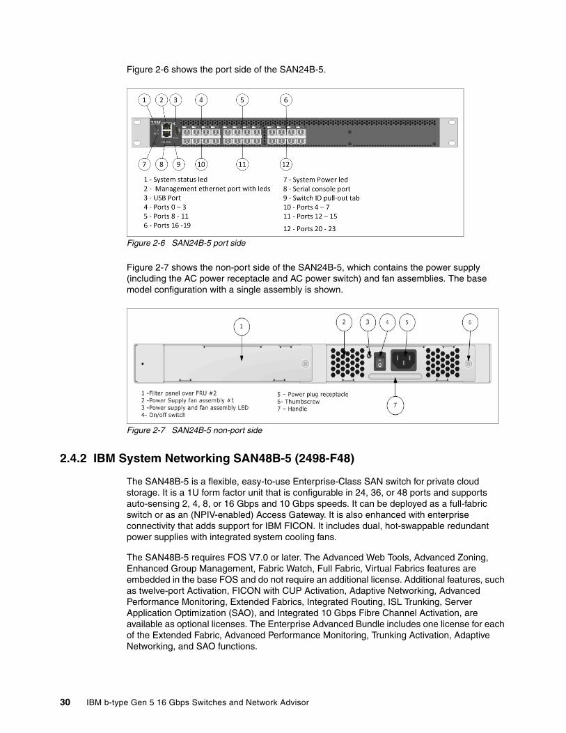
Figure 2-6 shows the port side of the SAN24B-5.
Figure 2-6 SAN24B-5 port side
Figure 2-7 shows the non-port side of the SAN24B-5, which contains the power supply (including the AC power receptacle and AC power switch) and fan assemblies. The base model configuration with a single assembly is shown.
Figure 2-7 SAN24B-5 non-port side
2.4.2 IBM System Networking SAN48B-5 (2498-F48)
The SAN48B-5 is a flexible, easy-to-use Enterprise-Class SAN switch for private cloud storage. It is a 1U form factor unit that is configurable in 24, 36, or 48 ports and supports auto-sensing 2, 4, 8, or 16 Gbps and 10 Gbps speeds. It can be deployed as a full-fabric switch or as an (NPIV-enabled) Access Gateway. It is also enhanced with enterprise connectivity that adds support for IBM FICON. It includes dual, hot-swappable redundant power supplies with integrated system cooling fans.
The SAN48B-5 requires FOS V7.0 or later. The Advanced Web Tools, Advanced Zoning, Enhanced Group Management, Fabric Watch, Full Fabric, Virtual Fabrics features are embedded in the base FOS and do not require an additional license. Additional features, such as twelve-port Activation, FICON with CUP Activation, Adaptive Networking, Advanced Performance Monitoring, Extended Fabrics, Integrated Routing, ISL Trunking, Server Application Optimization (SAO), and Integrated 10 Gbps Fibre Channel Activation, are available as optional licenses. The Enterprise Advanced Bundle includes one license for each of the Extended Fabric, Advanced Performance Monitoring, Trunking Activation, Adaptive Networking, and SAO functions.
30 IBM b-type Gen 5 16 Gbps Switches and Network Advisor

SAN48B-5 provides the following features and benefits:
� Up to 48 16 Gbps auto-sensing ports in an energy-efficient 1U form factor.
� Ports on Demand (PoD) licensing capabilities for scaling (24 - 48 ports in 12-port increments).
� Supports 2, 4, 8, and 16 Gbps auto-sensing Fibre Channel switch and router ports. 2, 4, and 8 Gbps performance is enabled by 8 Gbps SFP+ transceivers:
– 4, 8, and 16 Gbps performance is enabled by 16 Gbps SFP+ transceivers.
– 10 Gbps manual set capability on FC ports (requires the optional 10 Gigabit FCIP/Fibre Channel license).
– 10 Gbps performance is enabled by 10 Gbps SFP+ transceivers.
– Ports can be configured for 10 Gbps for metro connectivity2
� Gen 5 16 Gbps optimized Inter-Switch Link (ISL). Inter-Switch Link (ISL) Trunking3, which allows up to eight ports (at 2, 4, 8, or 16 Gbps speeds) between a pair of switches to combine to form a single logical ISL with a speed of up to 128 Gbps (256 Gbps full duplex) for optimal bandwidth usage and load balancing.
� Universal ports self-configure as E, F, M, or D ports. EX_Ports can be activated on a per port basis with the optional Integrated Routing license.
� The Diagnostic Port (D-Port) feature provides physical media diagnostic, troubleshooting, and verification services.
� In-flight data compression and encryption on up to two ports provides efficient link usage and security.
� Options for port side exhaust (default) or non-port side exhaust airflow for cooling.
� Virtual Fabric support to improve isolation between different VFs.
� Fibre Channel Routing (FCR) service, available with the optional Integrated Routing license, provides improved scalability and fault isolation.
� FICON, FICON Cascading, and FICON Control Unit Port ready.
� Dynamic Path Selection (DPS), which optimizes fabric-wide performance and load balancing by automatically routing data to the most efficient available path in the fabric.
� Brocade-branded SFP+ optical transceivers, which support any combination of Short Wavelength (SWL), Long Wavelength (LWL), or Extended Long Wavelength (ELWL) optical media among the switch ports.
� Extended distance support enables native Fibre Channel extension up to 7,500 km at 2 Gbps.
� Support for unicast, multicast (255 groups), and broadcast data traffic types.
� Support for an Access Gateway configuration where server ports that are connected to the fabric core are virtualized.
� Extensive diagnostic and system-monitoring capabilities for enhanced high reliability, availability, and serviceability (RAS).
� 10G Fibre Channel integration on the same port provides for DWDM metro connectivity on the same switch (can be done on the first eight ports only).
� The EZSwitchSetup wizard makes SAN configuration a three-step point-and-click task.
2 Only the first eight ports can be used as Metro Mirror.3 Trunking is a licensable feature.
Chapter 2. Product hardware and features 31
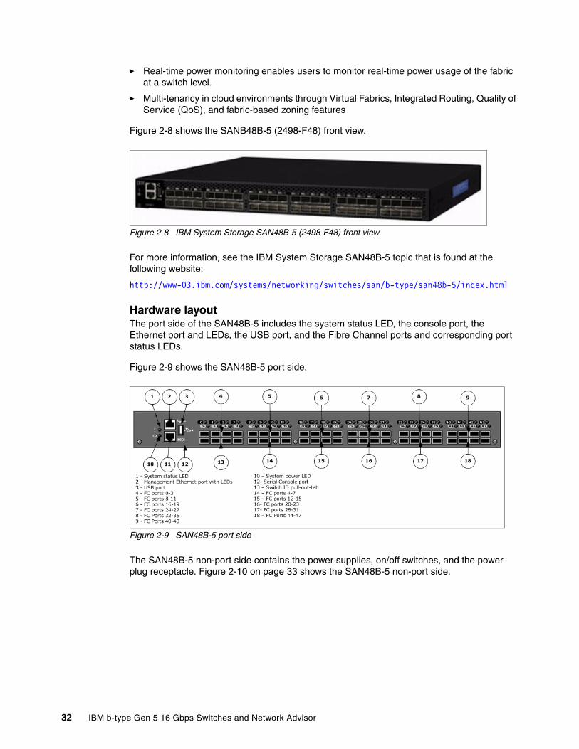
� Real-time power monitoring enables users to monitor real-time power usage of the fabric at a switch level.
� Multi-tenancy in cloud environments through Virtual Fabrics, Integrated Routing, Quality of Service (QoS), and fabric-based zoning features
Figure 2-8 shows the SANB48B-5 (2498-F48) front view.
Figure 2-8 IBM System Storage SAN48B-5 (2498-F48) front view
For more information, see the IBM System Storage SAN48B-5 topic that is found at the following website:
http://www-03.ibm.com/systems/networking/switches/san/b-type/san48b-5/index.html
Hardware layout The port side of the SAN48B-5 includes the system status LED, the console port, the Ethernet port and LEDs, the USB port, and the Fibre Channel ports and corresponding port status LEDs.
Figure 2-9 shows the SAN48B-5 port side.
Figure 2-9 SAN48B-5 port side
The SAN48B-5 non-port side contains the power supplies, on/off switches, and the power plug receptacle. Figure 2-10 on page 33 shows the SAN48B-5 non-port side.
32 IBM b-type Gen 5 16 Gbps Switches and Network Advisor
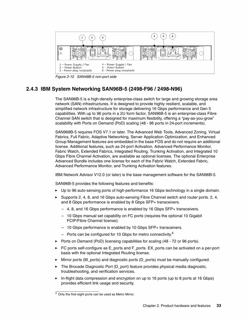
Figure 2-10 SAN48B-5 non-port side
2.4.3 IBM System Networking SAN96B-5 (2498-F96 / 2498-N96)
The SAN96B-5 is a high-density enterprise-class switch for large and growing storage area network (SAN) infrastructures. It is designed to provide highly resilient, scalable, and simplified network infrastructure for storage delivering 16 Gbps performance and Gen 5 capabilities. With up to 96 ports in a 2U form factor, SAN96B-5 is an enterprise-class Fibre Channel SAN switch that is designed for maximum flexibility, offering a “pay-as-you-grow” scalability with Ports on Demand (PoD) scaling (48 - 96 ports in 24-port increments).
SAN968B-5 requires FOS V7.1 or later. The Advanced Web Tools, Advanced Zoning, Virtual Fabrics, Full Fabric, Adaptive Networking, Server Application Optimization, and Enhanced Group Management features are embedded in the base FOS and do not require an additional license. Additional features, such as 24-port Activation, Advanced Performance Monitor, Fabric Watch, Extended Fabrics, Integrated Routing, Trunking Activation, and Integrated 10 Gbps Fibre Channel Activation, are available as optional licenses. The optional Enterprise Advanced Bundle includes one license for each of the Fabric Watch, Extended Fabric, Advanced Performance Monitor, and Trunking Activation features.
IBM Network Advisor V12.0 (or later) is the base management software for the SAN96B-5.
SAN96B-5 provides the following features and benefits:
� Up to 96 auto-sensing ports of high-performance 16 Gbps technology in a single domain.
� Supports 2, 4, 8, and 16 Gbps auto-sensing Fibre Channel switch and router ports. 2, 4, and 8 Gbps performance is enabled by 8 Gbps SFP+ transceivers.
– 4, 8, and 16 Gbps performance is enabled by 16 Gbps SFP+ transceivers.
– 10 Gbps manual set capability on FC ports (requires the optional 10 Gigabit FCIP/Fibre Channel license).
– 10 Gbps performance is enabled by 10 Gbps SFP+ transceivers.
– Ports can be configured for 10 Gbps for metro connectivity.4
� Ports on Demand (PoD) licensing capabilities for scaling (48 - 72 or 96 ports).
� FC ports self-configure as E_ports and F_ports. EX_ports can be activated on a per-port basis with the optional Integrated Routing license.
� Mirror ports (M_ports) and diagnostic ports (D_ports) must be manually configured.
� The Brocade Diagnostic Port (D_port) feature provides physical media diagnostic, troubleshooting, and verification services.
� In-flight data compression and encryption on up to 16 ports (up to 8 ports at 16 Gbps) provides efficient link usage and security.
4 Only the first eight ports can be used as Metro Mirror.
Chapter 2. Product hardware and features 33
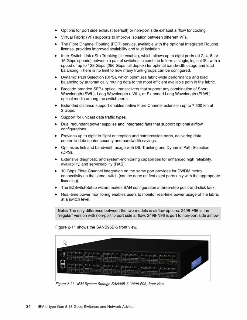
� Options for port side exhaust (default) or non-port side exhaust airflow for cooling.
� Virtual Fabric (VF) supports to improve isolation between different VFs.
� The Fibre Channel Routing (FCR) service, available with the optional Integrated Routing license, provides improved scalability and fault isolation.
� Inter-Switch Link (ISL) Trunking (licensable), which allows up to eight ports (at 2, 4, 8, or 16 Gbps speeds) between a pair of switches to combine to form a single, logical ISL with a speed of up to 128 Gbps (256 Gbps full duplex) for optimal bandwidth usage and load balancing. There is no limit to how many trunk groups can be configured.
� Dynamic Path Selection (DPS), which optimizes fabric-wide performance and load balancing by automatically routing data to the most efficient available path in the fabric.
� Brocade-branded SFP+ optical transceivers that support any combination of Short Wavelength (SWL), Long Wavelength (LWL), or Extended Long Wavelength (ELWL) optical media among the switch ports.
� Extended distance support enables native Fibre Channel extension up to 7,500 km at 2 Gbps.
� Support for unicast data traffic types.
� Dual redundant power supplies and integrated fans that support optional airflow configurations.
� Provides up to eight in-flight encryption and compression ports, delivering data center-to-data center security and bandwidth savings.
� Optimizes link and bandwidth usage with ISL Trunking and Dynamic Path Selection (DPS).
� Extensive diagnostic and system-monitoring capabilities for enhanced high reliability, availability, and serviceability (RAS).
� 10 Gbps Fibre Channel integration on the same port provides for DWDM metro connectivity on the same switch (can be done on first eight ports only with the appropriate licensing).
� The EZSwitchSetup wizard makes SAN configuration a three-step point-and-click task.
� Real-time power monitoring enables users to monitor real-time power usage of the fabric at a switch level.
Figure 2-11 shows the SANB96B-5 front view.
Figure 2-11 IBM System Storage SAN96B-5 (2498-F96) front view
Note: The only difference between the two models is airflow options. 2498-F96 is the “regular” version with non-port to port side airflow; 2498-N96 is port to non-port side airflow
34 IBM b-type Gen 5 16 Gbps Switches and Network Advisor

For more information, see the IBM System Storage SAN96B-5 topic that is found at the following website:
http://www-03.ibm.com/systems/networking/switches/san/b-type/san96b-5/index.html
Hardware layoutThe port side of the SAN96B-5 includes the system status LED, the console port, the Ethernet port and accompanying LEDs, the USB port, and the Fibre Channel ports and corresponding port status LEDs.
Figure 2-12 shows the SAN96B-5 port side view.
Figure 2-12 SAN96B-5 port side view
The SAN96B5 non-port side contains the power supplies (including the AC power receptacle) and fans.
Figure 2-13 shows the non-port side of the SAN96B-5.
Figure 2-13 SAN96B-5 non-port side view
Chapter 2. Product hardware and features 35
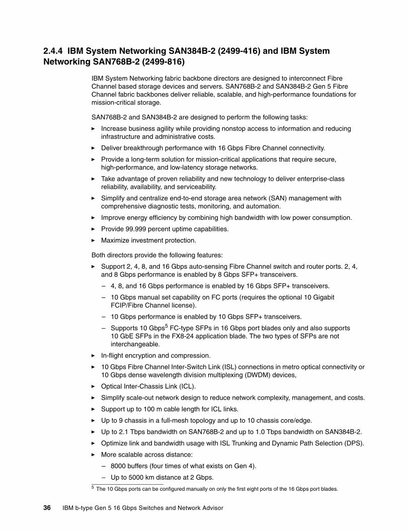
2.4.4 IBM System Networking SAN384B-2 (2499-416) and IBM System Networking SAN768B-2 (2499-816)
IBM System Networking fabric backbone directors are designed to interconnect Fibre Channel based storage devices and servers. SAN768B-2 and SAN384B-2 Gen 5 Fibre Channel fabric backbones deliver reliable, scalable, and high-performance foundations for mission-critical storage.
SAN768B-2 and SAN384B-2 are designed to perform the following tasks:
� Increase business agility while providing nonstop access to information and reducing infrastructure and administrative costs.
� Deliver breakthrough performance with 16 Gbps Fibre Channel connectivity.
� Provide a long-term solution for mission-critical applications that require secure, high-performance, and low-latency storage networks.
� Take advantage of proven reliability and new technology to deliver enterprise-class reliability, availability, and serviceability.
� Simplify and centralize end-to-end storage area network (SAN) management with comprehensive diagnostic tests, monitoring, and automation.
� Improve energy efficiency by combining high bandwidth with low power consumption.
� Provide 99.999 percent uptime capabilities.
� Maximize investment protection.
Both directors provide the following features:
� Support 2, 4, 8, and 16 Gbps auto-sensing Fibre Channel switch and router ports. 2, 4, and 8 Gbps performance is enabled by 8 Gbps SFP+ transceivers.
– 4, 8, and 16 Gbps performance is enabled by 16 Gbps SFP+ transceivers.
– 10 Gbps manual set capability on FC ports (requires the optional 10 Gigabit FCIP/Fibre Channel license).
– 10 Gbps performance is enabled by 10 Gbps SFP+ transceivers.
– Supports 10 Gbps5 FC-type SFPs in 16 Gbps port blades only and also supports 10 GbE SFPs in the FX8-24 application blade. The two types of SFPs are not interchangeable.
� In-flight encryption and compression.
� 10 Gbps Fibre Channel Inter-Switch Link (ISL) connections in metro optical connectivity or 10 Gbps dense wavelength division multiplexing (DWDM) devices,
� Optical Inter-Chassis Link (ICL).
� Simplify scale-out network design to reduce network complexity, management, and costs.
� Support up to 100 m cable length for ICL links.
� Up to 9 chassis in a full-mesh topology and up to 10 chassis core/edge.
� Up to 2.1 Tbps bandwidth on SAN768B-2 and up to 1.0 Tbps bandwidth on SAN384B-2.
� Optimize link and bandwidth usage with ISL Trunking and Dynamic Path Selection (DPS).
� More scalable across distance:
– 8000 buffers (four times of what exists on Gen 4).
– Up to 5000 km distance at 2 Gbps.5 The 10 Gbps ports can be configured manually on only the first eight ports of the 16 Gbps port blades.
36 IBM b-type Gen 5 16 Gbps Switches and Network Advisor
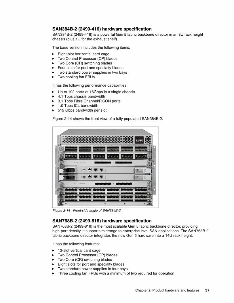
SAN384B-2 (2499-416) hardware specificationSAN384B-2 (2499-416) is a powerful Gen 5 fabric backbone director in an 8U rack height chassis (plus 1U for the exhaust shelf).
The base version includes the following items:
� Eight-slot horizontal card cage� Two Control Processor (CP) blades� Two Core (CR) switching blades� Four slots for port and specialty blades� Two standard power supplies in two bays� Two cooling fan FRUs
It has the following performance capabilities:
� Up to 192 ports at 16Gbps in a single chassis� 4.1 Tbps chassis bandwidth� 3.1 Tbps Fibre Channel/FICON ports� 1.0 Tbps ICL bandwidth� 512 Gbps bandwidth per slot
Figure 2-14 shows the front view of a fully populated SAN384B-2.
Figure 2-14 Front-side angle of SAN384B-2
SAN768B-2 (2499-816) hardware specificationSAN768B-2 (2499-816) is the most scalable Gen 5 fabric backbone director, providing high-port density. It supports midrange to enterprise level SAN applications. The SAN768B-2 fabric backbone director integrates the new Gen 5 hardware into a 14U rack height.
It has the following features:
� 12-slot vertical card cage� Two Control Processor (CP) blades� Two Core (CR) switching blades� Eight slots for port and specialty blades� Two standard power supplies in four bays� Three cooling fan FRUs with a minimum of two required for operation
Chapter 2. Product hardware and features 37

It has the following performance capabilities:
� Up to 384 ports at full 16 Gbps speed or up to 512 8 Gbps Fibre Channel ports� Up to 32 optical UltraScale ICL ports� 8.2 Tbps total chassis bandwidth:
– 6.1 Tbps Fibre Channel/FICON ports– 2.1 Tbps UltraScale ICL bandwidth– 512 Gbps bandwidth per slot
Figure 2-15 shows the front view of a fully populated SAN768B-2.
Figure 2-15 Front-side angle of SAN768B-2
For the latest information about SAN384B-2 and SAN768B-2, go to the following website:
http://www.ibm.com/systems/networking/switches/san/b-type/san768b/index.html
Blade support matrixThe IBM System Storage fabric backbone architectures support various blades and provide flexibility for different port density needs, multiprotocol capabilities, and fabric-based applications. Data center administrators can easily mix the blades to address specific business requirements and optimize cost/performance ratios.
The SAN768B-2 is a 12-slot chassis consisting of 8-port blades, two control processor (CP8) blades, and two core (CR8) blades, as shown in Figure 2-16 on page 39.
38 IBM b-type Gen 5 16 Gbps Switches and Network Advisor

Figure 2-16 SAN768B-2 front view
The SAN384B-2 is an 8-slot chassis consisting of 4-port blades, two control processor (CP8) blades, and two core (CR8) blades, as shown in Figure 2-17.
Figure 2-17 SAN384B-2 front view
The Gen 5 and Gen 4 directors have different blade compatibility, as described 2.4.5, “IBM Fabric backbone blades” on page 40.
Chapter 2. Product hardware and features 39
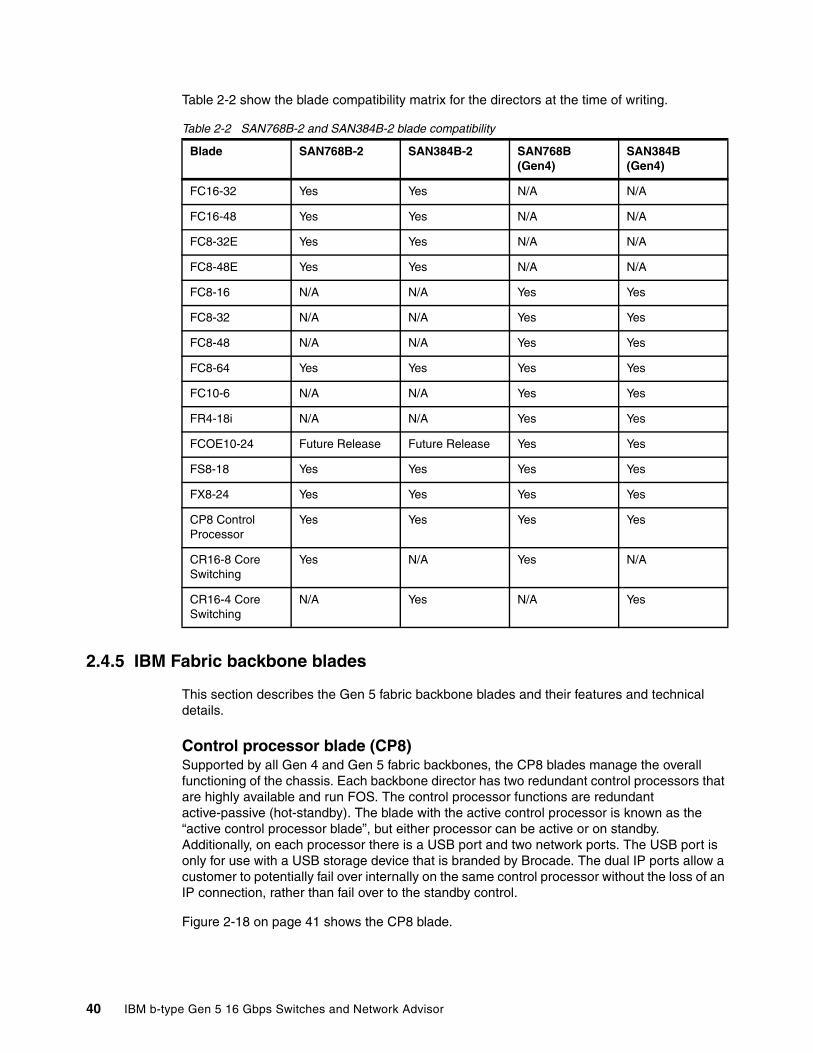
Table 2-2 show the blade compatibility matrix for the directors at the time of writing.
Table 2-2 SAN768B-2 and SAN384B-2 blade compatibility
2.4.5 IBM Fabric backbone blades
This section describes the Gen 5 fabric backbone blades and their features and technical details.
Control processor blade (CP8)Supported by all Gen 4 and Gen 5 fabric backbones, the CP8 blades manage the overall functioning of the chassis. Each backbone director has two redundant control processors that are highly available and run FOS. The control processor functions are redundant active-passive (hot-standby). The blade with the active control processor is known as the “active control processor blade”, but either processor can be active or on standby. Additionally, on each processor there is a USB port and two network ports. The USB port is only for use with a USB storage device that is branded by Brocade. The dual IP ports allow a customer to potentially fail over internally on the same control processor without the loss of an IP connection, rather than fail over to the standby control.
Figure 2-18 on page 41 shows the CP8 blade.
Blade SAN768B-2 SAN384B-2 SAN768B (Gen4)
SAN384B (Gen4)
FC16-32 Yes Yes N/A N/A
FC16-48 Yes Yes N/A N/A
FC8-32E Yes Yes N/A N/A
FC8-48E Yes Yes N/A N/A
FC8-16 N/A N/A Yes Yes
FC8-32 N/A N/A Yes Yes
FC8-48 N/A N/A Yes Yes
FC8-64 Yes Yes Yes Yes
FC10-6 N/A N/A Yes Yes
FR4-18i N/A N/A Yes Yes
FCOE10-24 Future Release Future Release Yes Yes
FS8-18 Yes Yes Yes Yes
FX8-24 Yes Yes Yes Yes
CP8 Control Processor
Yes Yes Yes Yes
CR16-8 Core Switching
Yes N/A Yes N/A
CR16-4 Core Switching
N/A Yes N/A Yes
40 IBM b-type Gen 5 16 Gbps Switches and Network Advisor

Figure 2-18 CP8 blade
Core routing blades (CR16-8 and CR16-4)The Gen 5 fabric backbone includes two core routing blades for SAN384B-2 (CR16-4, which is shown in Figure 2-19 on page 42) or SAN768B-2 (CR16-8, which is shown in Figure 2-20 on page 42). These blades provide core switching and routing of the frames either from blade to blade or from the fabric backbone chassis through the ICL ports. The CR16-8 and CR16-4 blades work as an active-active cluster.
The CR16-8 has four Condor3 ASICs. The CR16-4 has two Condor3 ASICs. Each ASIC has dual connections to each ASIC group on each line card.
Here are the CR16-4 blade hardware features:
� Two Condor3 ASICs� Eight QSFP (ICL) ports� Up to 1 Tbps backplane throughput
Chapter 2. Product hardware and features 41

Figure 2-19 shows the CR16-4 core blade.
Figure 2-19 CR16-4 Core Blade
Here are the CR16-8 blade hardware features:
� Three Condor3 ASICs� Sixteen QSFP (ICL) ports� Up to 2 Tbps backplane throughput
Figure 2-20 shows the CR16-8 core blade.
Figure 2-20 CR16-8 core blade
42 IBM b-type Gen 5 16 Gbps Switches and Network Advisor

FC16-32 32-port 16 Gbps bladeThe FC16-32 port blade is equipped with two Condor3 ASICs and can operate at a 16-Gbps full-line rate through the backplane or with local switching with no oversubscription (1:1).
It has the following hardware features:
� Two Condor3 ASICs� 16x 16 Gbps ports per ASIC� 512 Gbps backplane throughput� No oversubscription at 16 Gbps (1:1)
Figure 2-21 shows the FC16-32 port blade.
Figure 2-21 FC16-32 port blade
FC16-48 48-port 16 Gbps bladeThe FC16-48 port blade is equipped with two Condor3 ASICs, with one ASIC for each 24-port group. Although the backplane connectivity of this blade is identical to the FC16-32 blade, the FC16-48 blade uses 24 user-facing ports per ASIC rather than 16.
Oversubscription occurs only when the first 32 ports are fully used (16 Gbps) with no local switching.
It has the following hardware features:
� Two Condor3 ASICs� 24x 16 Gbps ports per ASIC� 512 Gbps backplane throughput� 1.5:1 oversubscription at 16 Gbps
Note: The CR core blades are also responsible for routing ICL frames from backbone chassis. ICLs are described in 2.4.6, “Optical UltraScale Inter-Chassis Links” on page 49.
Chapter 2. Product hardware and features 43

Figure 2-22 shows the FC16-48 port blade.
Figure 2-22 FC16-48 port blade
FC8-64 64-port 8 Gbps bladeEquipped with four Condor2 ASICs, the FC8-64 port blade offers 64x 8 Gbps ports (16 ports per ASIC) and provides a 2:1 oversubscription ratio at 8 Gbps switching through the backplane and no oversubscription with local switching.
It has the following key features:
� Four Condor2 ASICs � 16x 8 Gbps ports per ASIC� 256 Gbps backplane throughput� 64 front-end ports and 32 back-end ports, 2:1 oversubscription, and no oversubscription
with local switching
Figure 2-23 on page 45 shows the FC8-64 port blade.
44 IBM b-type Gen 5 16 Gbps Switches and Network Advisor

Figure 2-23 FC8-64 port blade
FC8-32E 32-port Enhanced 8 Gbps bladeEquipped with two Condor3 ASICs, the FC8-32E port blade offers 328 Gbps front-end ports and 32 back-end ports and no oversubscription at 8 Gbps switching through the backplane. FC8-32E supports E, F, M, and EX Fibre Channel ports and can operate at 2, 4, and 8 Gbps.
Chapter 2. Product hardware and features 45

Figure 2-24 shows the FC8-32E port blade.
Figure 2-24 FC8-32E port blade
FC8-48E 48-port Enhanced 8 Gbps bladeEquipped with two Condor3 ASICs, the FC8-48E port blade offers 48x 8 Gbps front-end ports and 32 back-end ports and no oversubscription at 8 Gbps switching through the backplane. FC8-48E supports E, F, M, and EX Fibre Channel ports and can operate at 2, 4, and 8 Gbps.
Figure 2-25 on page 47 shows the FC8-48E port blade.
46 IBM b-type Gen 5 16 Gbps Switches and Network Advisor
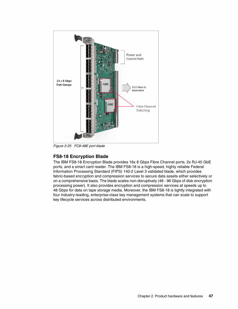
Figure 2-25 FC8-48E port blade
FS8-18 Encryption BladeThe IBM FS8-18 Encryption Blade provides 16x 8 Gbps Fibre Channel ports, 2x RJ-45 GbE ports, and a smart card reader. The IBM FS8-18 is a high-speed, highly reliable Federal Information Processing Standard (FIPS) 140-2 Level 3 validated blade, which provides fabric-based encryption and compression services to secure data assets either selectively or on a comprehensive basis. The blade scales non-disruptively (48 - 96 Gbps of disk encryption processing power). It also provides encryption and compression services at speeds up to 48 Gbps for data on tape storage media. Moreover, the IBM FS8-18 is tightly integrated with four industry-leading, enterprise-class key management systems that can scale to support key lifecycle services across distributed environments.
Chapter 2. Product hardware and features 47

Figure 2-26 shows the IBM FS8-18 Encryption Blade
Figure 2-26 FS8-18 Encryption Blade
FX8-24 Extension Blade The IBM FX8-24 Extension Blade accelerates and optimizes replication, backup, and migration over any distance. The twelve 8 Gbps Fibre Channel ports, ten 1 GbE ports, and up to two optional 10 GbE ports provide Fibre Channel and FCIP bandwidth, port density, and throughput for maximum application performance over IP WAN links.
Figure 2-27 on page 49 shows the FX8-24 Extension Blade.
48 IBM b-type Gen 5 16 Gbps Switches and Network Advisor
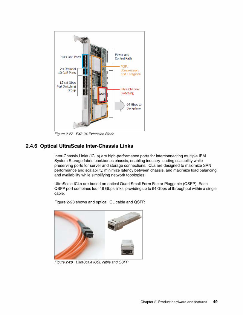
Figure 2-27 FX8-24 Extension Blade
2.4.6 Optical UltraScale Inter-Chassis Links
Inter-Chassis Links (ICLs) are high-performance ports for interconnecting multiple IBM System Storage fabric backbones chassis, enabling industry-leading scalability while preserving ports for server and storage connections. ICLs are designed to maximize SAN performance and scalability, minimize latency between chassis, and maximize load balancing and availability while simplifying network topologies.
UltraScale ICLs are based on optical Quad Small Form Factor Pluggable (QSFP). Each QSFP port combines four 16 Gbps links, providing up to 64 Gbps of throughput within a single cable.
Figure 2-28 shows and optical ICL cable and QSFP.
Figure 2-28 UltraScale ICSL cable and QSFP
Chapter 2. Product hardware and features 49
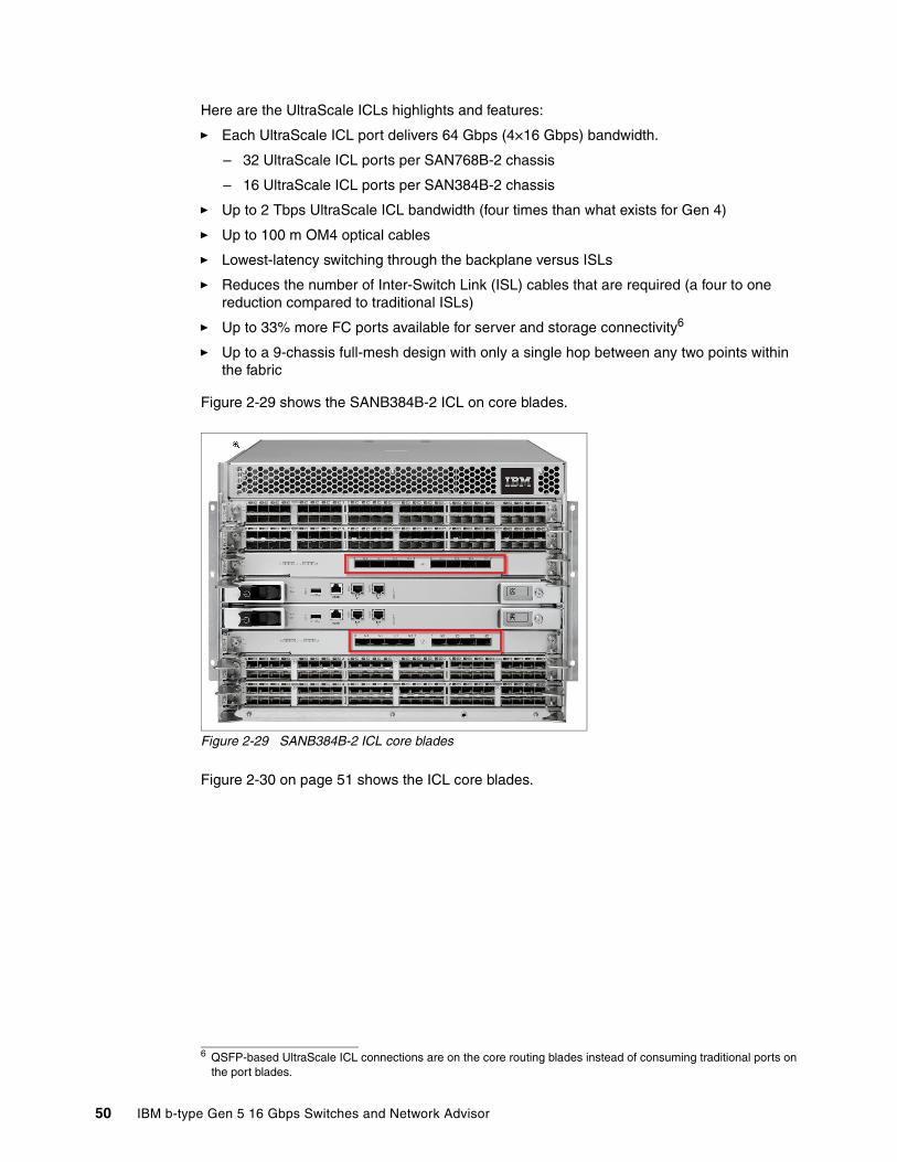
Here are the UltraScale ICLs highlights and features:
� Each UltraScale ICL port delivers 64 Gbps (4×16 Gbps) bandwidth.
– 32 UltraScale ICL ports per SAN768B-2 chassis
– 16 UltraScale ICL ports per SAN384B-2 chassis
� Up to 2 Tbps UltraScale ICL bandwidth (four times than what exists for Gen 4)
� Up to 100 m OM4 optical cables
� Lowest-latency switching through the backplane versus ISLs
� Reduces the number of Inter-Switch Link (ISL) cables that are required (a four to one reduction compared to traditional ISLs)
� Up to 33% more FC ports available for server and storage connectivity6
� Up to a 9-chassis full-mesh design with only a single hop between any two points within the fabric
Figure 2-29 shows the SANB384B-2 ICL on core blades.
Figure 2-29 SANB384B-2 ICL core blades
Figure 2-30 on page 51 shows the ICL core blades.
6 QSFP-based UltraScale ICL connections are on the core routing blades instead of consuming traditional ports on the port blades.
50 IBM b-type Gen 5 16 Gbps Switches and Network Advisor
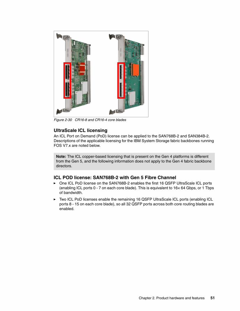
Figure 2-30 CR16-8 and CR16-4 core blades
UltraScale ICL licensingAn ICL Port on Demand (PoD) license can be applied to the SAN768B-2 and SAN384B-2. Descriptions of the applicable licensing for the IBM System Storage fabric backbones running FOS V7.x are noted below.
ICL POD license: SAN768B-2 with Gen 5 Fibre Channel� One ICL PoD license on the SAN768B-2 enables the first 16 QSFP UltraScale ICL ports
(enabling ICL ports 0 - 7 on each core blade). This is equivalent to 16× 64 Gbps, or 1 Tbps of bandwidth.
� Two ICL PoD licenses enable the remaining 16 QSFP UltraScale ICL ports (enabling ICL ports 8 - 15 on each core blade), so all 32 QSFP ports across both core routing blades are enabled.
Note: The ICL copper-based licensing that is present on the Gen 4 platforms is different from the Gen 5, and the following information does not apply to the Gen 4 fabric backbone directors.
Chapter 2. Product hardware and features 51

Figure 2-31 shows the CR16-8 core blade and ICL ports.
Figure 2-31 CR16-8 core blade
ICL PoD license: SAN384B-2 with Gen 5 Fibre ChannelOnly one ICL PoD license is required to enable all 16 QSFP UltraScale ICL ports that are available on the two core blades of the SAN384B-2. This is equivalent to 16× 64 Gbps, or 1 Tbps of bandwidth.
Enterprise ICL (EICL) license: SAN768B-2 and SAN384B-2 with Gen 5 Fibre ChannelThe EICL license is required on each IBM System Storage fabric backbone chassis that connects to four or more chassis through UltraScale ICLs. This license requirement does not depend upon the total number of chassis that exist in a fabric, but only on how many chassis are directly connected through ICLs. This license is in addition to the ICL PoD license requirements, which enable the actual ICL ports.
52 IBM b-type Gen 5 16 Gbps Switches and Network Advisor
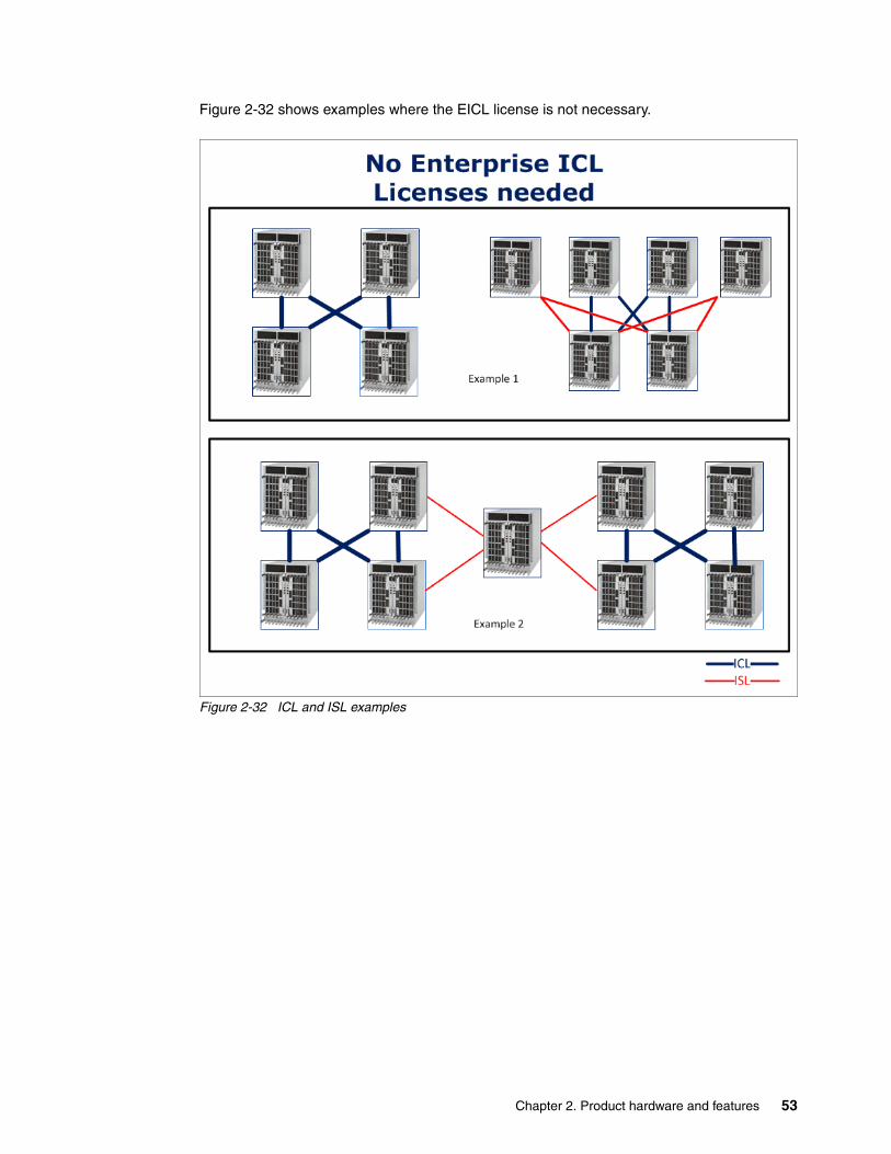
Figure 2-32 shows examples where the EICL license is not necessary.
Figure 2-32 ICL and ISL examples
Chapter 2. Product hardware and features 53
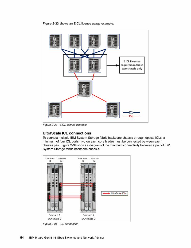
Figure 2-33 shows an EICL license usage example.
Figure 2-33 EICL license example
UltraScale ICL connectionsTo connect multiple IBM System Storage fabric backbone chassis through optical ICLs, a minimum of four ICL ports (two on each core blade) must be connected between each chassis pair. Figure 2-34 shows a diagram of the minimum connectivity between a pair of IBM System Storage fabric backbone chassis.
Figure 2-34 ICL connection
54 IBM b-type Gen 5 16 Gbps Switches and Network Advisor

SAN768B-2 has 32 ICL ports available (with both ICL PoD licenses installed), which supports ICL connectivity to up to eight other chassis and at least 256 Gbps of bandwidth to each connected SAN768B-2.
SAN384B-2 has 16 ICL ports available, which supports up to four chassis and at least 128 Gbps of bandwidth to each connected SAN384B-2.
With 32 ICL ports available on the SAN768B-2 (with both ICL PoD licenses installed) and 16 ICL ports on SAN384B-2, these configurations support ICL connectivity to up to eight other chassis and at least 256 Gbps of bandwidth to each connected SAN768B-2.
A maximum of 16 UltraScale ICL connections or ICL trunk groups between any pair of IBM System Storage fabric backbone chassis is supported, unless they are deployed using Virtual Fabrics, where a maximum of 16 ICL connections or trunks can be assigned to a single Logical Switch. This limitation is because of the maximum supported number of connections for Fabric Shortest Path First (FSPF) routing. Effectively, this means that there should never be more than 16 ICL connections or trunks between a pair of SAN768B-2 chassis, unless Virtual Fabrics is enabled, and the ICLs are assigned to two or more Logical Switches. The exception to this situation is if eight port trunks are created between a pair of SAN768B-2 chassis. Details about this configuration are described in “Ultrascale ICL trunking and trunk groups”.
Ultrascale ICL trunking and trunk groupsTrunking involves taking multiple physical connections between a chassis or switch pair and forming a single “virtual” connection and aggregating the bandwidth for traffic to traverse. There are different hardware-based trunking solutions, including the ISL Trunking for traditional ISLs, trunking for Integrated Routing (FCR connectivity), trunking for Access Gateway, and also trunking for UltraScale ICLs. This section describes the trunking capability that is used with the QSFP-based UltraScale ICL ports on the IBM System Storage fabric backbone. For ISL Trunking, see 2.5.2, “ISL Trunking” on page 57.
Each optical ICL port has four independent 16-Gbps links, each of which terminates on one of four ASICs on each SAN768B-2 core blade, or two ASICs on each SAN384B-2 core blade. Trunk groups can be formed by using any of the ports that comprise contiguous groups of eight links on each ASIC.
Note: If more than four ICL connections are required between a pair of IBM System Storage fabric backbones, additional ICL connections should be added in pairs (one on each core blade).
Note: QSFP-based UltraScale ICLs and traditional ISLs are not concurrently supported between a single pair of IBM System Storage fabric backbone chassis. All inter-chassis connectivity between any pair of IBM System Storage fabric backbone chassis must be done by using either ISLs or UltraScale ICLs.
Chapter 2. Product hardware and features 55
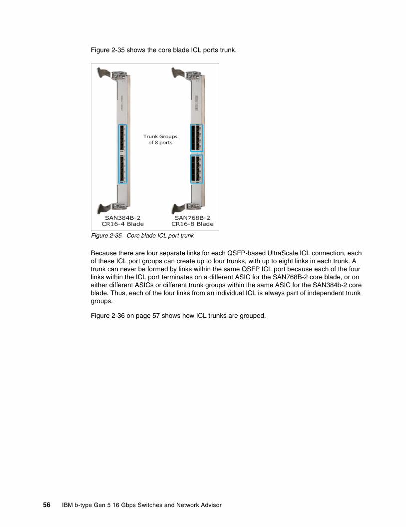
Figure 2-35 shows the core blade ICL ports trunk.
Figure 2-35 Core blade ICL port trunk
Because there are four separate links for each QSFP-based UltraScale ICL connection, each of these ICL port groups can create up to four trunks, with up to eight links in each trunk. A trunk can never be formed by links within the same QSFP ICL port because each of the four links within the ICL port terminates on a different ASIC for the SAN768B-2 core blade, or on either different ASICs or different trunk groups within the same ASIC for the SAN384b-2 core blade. Thus, each of the four links from an individual ICL is always part of independent trunk groups.
Figure 2-36 on page 57 shows how ICL trunks are grouped.
56 IBM b-type Gen 5 16 Gbps Switches and Network Advisor
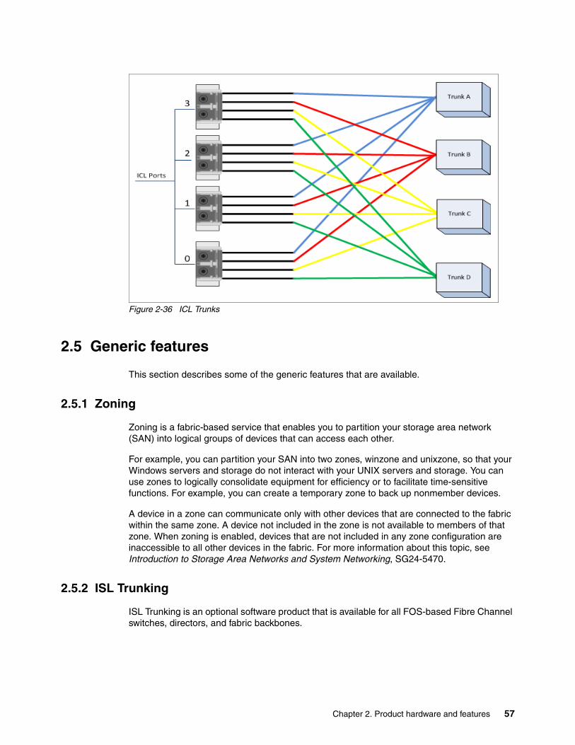
Figure 2-36 ICL Trunks
2.5 Generic features
This section describes some of the generic features that are available.
2.5.1 Zoning
Zoning is a fabric-based service that enables you to partition your storage area network (SAN) into logical groups of devices that can access each other.
For example, you can partition your SAN into two zones, winzone and unixzone, so that your Windows servers and storage do not interact with your UNIX servers and storage. You can use zones to logically consolidate equipment for efficiency or to facilitate time-sensitive functions. For example, you can create a temporary zone to back up nonmember devices.
A device in a zone can communicate only with other devices that are connected to the fabric within the same zone. A device not included in the zone is not available to members of that zone. When zoning is enabled, devices that are not included in any zone configuration are inaccessible to all other devices in the fabric. For more information about this topic, see Introduction to Storage Area Networks and System Networking, SG24-5470.
2.5.2 ISL Trunking
ISL Trunking is an optional software product that is available for all FOS-based Fibre Channel switches, directors, and fabric backbones.
Chapter 2. Product hardware and features 57
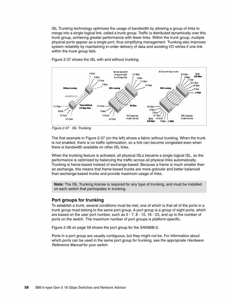
ISL Trunking technology optimizes the usage of bandwidth by allowing a group of links to merge into a single logical link, called a trunk group. Traffic is distributed dynamically over this trunk group, achieving greater performance with fewer links. Within the trunk group, multiple physical ports appear as a single port, thus simplifying management. Trunking also improves system reliability by maintaining in-order delivery of data and avoiding I/O retries if one link within the trunk group fails.
Figure 2-37 shows the ISL with and without trunking.
Figure 2-37 ISL Trunking
The first example in Figure 2-37 (on the left) shows a fabric without trunking. When the trunk is not enabled, there is no traffic optimization, so a link can become congested even when there is bandwidth available on other ISL links.
When the trunking feature is activated, all physical ISLs became a single logical ISL, so the performance is optimized by balancing the traffic across all physical links automatically. Trunking is frame-based instead of exchange-based. Because a frame is much smaller than an exchange, this means that frame-based trunks are more granular and better balanced than exchange-based trunks and provide maximum usage of links.
Port groups for trunkingTo establish a trunk, several conditions must be met, one of which is that all of the ports in a trunk group must belong to the same port group. A port group is a group of eight ports, which are based on the user port number, such as 0 - 7, 8 - 15, 16 - 23, and up to the number of ports on the switch. The maximum number of port groups is platform-specific.
Figure 2-38 on page 59 shows the port group for the SAN96B-5.
Ports in a port group are usually contiguous, but they might not be. For information about which ports can be used in the same port group for trunking, see the appropriate Hardware Reference Manual for your switch.
Note: The ISL Trunking license is required for any type of trunking, and must be installed on each switch that participates in trunking.
58 IBM b-type Gen 5 16 Gbps Switches and Network Advisor

Figure 2-38 SAN96B-5 port group
Supported configurations for trunkingHere are the supported configurations for trunking:
� Trunk links can be 2 Gbps, 4 Gbps, 8 Gbps, 10 Gbps, or 16 Gbps, depending on the b-type platform.
� The maximum number of ports per trunk and trunks per switch depends on the b-type platform.
� You can have up to eight ports in one trunk group to create high-performance ISL trunks between switches, providing up to 128 Gbps (based on a 16 Gbps port speed).
� If in-flight encryption/compression is enabled, you can have a maximum of only two ports per trunk.
� An E_Port or EX_Port trunk can be up to eight ports wide. All the ports must be adjacent to each other, in the clearly marked groups on the front of the product.
Trunks operate best when the cable length of each trunked link is roughly equal to the length of the others in the trunk. For optimal performance, no more than 30-meters difference is recommended. Trunks are compatible with both Short-Wavelength (SWL) and Long-Wavelength (LWL) fiber-optic cables and transceivers.
Trunking is performed according to the Quality of Service (QoS) configuration on the ports. That is, in a trunk group, if there are some ports with QoS enabled and some with QoS disabled, they form two different trunks: one with QoS enabled and the other with QoS disabled.
Requirements for trunk groupsThe following requirements apply to all types of trunking:
� The Trunking license must be installed on every switch that participates in trunking.
� All of the ports in a trunk group must belong to the same port group.
� All of the ports in a trunk group must meet the following conditions:
– They must be running at the same speed.
– They must be configured for the same distance.
– They must have the same encryption, compression, QoS, and FEC settings.
� Trunk groups must be between b-type switches. Trunking is not supported on M-EOS or third-party switches.
� There must be a direct connection between participating switches.
Chapter 2. Product hardware and features 59
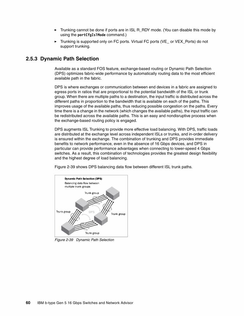
� Trunking cannot be done if ports are in ISL R_RDY mode. (You can disable this mode by using the portCfgIslMode command.)
� Trunking is supported only on FC ports. Virtual FC ports (VE_ or VEX_Ports) do not support trunking.
2.5.3 Dynamic Path Selection
Available as a standard FOS feature, exchange-based routing or Dynamic Path Selection (DPS) optimizes fabric-wide performance by automatically routing data to the most efficient available path in the fabric.
DPS is where exchanges or communication between end devices in a fabric are assigned to egress ports in ratios that are proportional to the potential bandwidth of the ISL or trunk group. When there are multiple paths to a destination, the input traffic is distributed across the different paths in proportion to the bandwidth that is available on each of the paths. This improves usage of the available paths, thus reducing possible congestion on the paths. Every time there is a change in the network (which changes the available paths), the input traffic can be redistributed across the available paths. This is an easy and nondisruptive process when the exchange-based routing policy is engaged.
DPS augments ISL Trunking to provide more effective load balancing. With DPS, traffic loads are distributed at the exchange level across independent ISLs or trunks, and in-order delivery is ensured within the exchange. The combination of trunking and DPS provides immediate benefits to network performance, even in the absence of 16 Gbps devices, and DPS in particular can provide performance advantages when connecting to lower-speed 4 Gbps switches. As a result, this combination of technologies provides the greatest design flexibility and the highest degree of load balancing.
Figure 2-39 shows DPS balancing data flow between different ISL trunk paths.
Figure 2-39 Dynamic Path Selection
60 IBM b-type Gen 5 16 Gbps Switches and Network Advisor
2.5.4 Port types
Here is a list of port types that may be part of a b-type device:
� D_Port: A diagnostic port lets an administrator isolate the ISL to diagnose link-level faults. This port runs only specific diagnostic tests and does not carry any fabric traffic. For more information, see “ClearLink Diagnostic Ports” on page 21.
� E_Port: An expansion port that is assigned to ISL links to expand a fabric by connecting it to other switches. Two connected E_Ports form an ISL. When E_Ports are used to connect switches, those switches merge into a single fabric without an isolation demarcation point. ISLs are non-routed links. For more information, see 2.5.2, “ISL Trunking” on page 57.
� EX_Port: A type of E_Port that connects a Fibre Channel router to an edge fabric. From the point of view of a switch in an edge fabric, an EX_Port appears as a normal E_Port. It follows applicable Fibre Channel standards like other E_Ports. However, the router terminates EX_Ports rather than allowing different fabrics to merge, which happens on a switch with regular E_Ports. An EX_Port cannot be connected to another EX_Port.
� F_Port: A fabric port that is assigned to fabric-capable devices, such as SAN storage devices.
� G_Port: A generic port that acts as a transition port for non-loop fabric-capable devices.
� L_/FL_Port: A loop or fabric loop port that connects loop devices. L_Ports are associated with private loop devices and FL_Ports are associated with public loop devices.
� M_Port: A mirror port that is configured to duplicate (mirror) the traffic passing between a specified source port and destination port. This is supported only for pairs of F_Ports. For more information about port mirroring, see the Fabric OS Troubleshooting and Diagnostics Guide, which you can find at the following website:
http://my.brocade.com/
� U_Port: A universal Fibre Channel port. This is the base Fibre Channel port type, and all unidentified or uninitiated ports are listed as U_Ports.
� VE_Port: A virtual E_Port that is a gigabit Ethernet switch port that is configured for an FCIP tunnel.
� VEX_Port: A virtual EX_Port that connects a Fibre Channel router to an edge fabric. From the point of view of a switch in an edge fabric, a VEX_Port appears as a normal VE_Port. It follows the same Fibre Channel protocol as other VE_Ports. However, the router terminates VEX_Ports rather than allowing different fabrics to merge, which is what happens on a switch with regular VE_Ports.
2.5.5 In-flight encryption and compression
The in-flight encryption and compression features of FOS allow frames to be encrypted or compressed at the egress point of an ISL between two IBM b-type switches, and then to be decrypted or extracted at the ingress point of the ISL. These features use port-based encryption and compression. You can enable the encryption and compression feature for both E_Ports and EX_Ports on a per-port basis. By default, this feature is initially disabled for all ports on a switch.
The purpose of encryption is to provide security for frames while they are in flight between two switches. The purpose of compression is for better bandwidth usage on the ISLs, especially over long distance. An average compression ratio of 2:1 is provided. Frames are never left in an encrypted or compressed state when delivered to an end device. Both ends of the ISL must terminate in 16G-capable FC ports.
Chapter 2. Product hardware and features 61
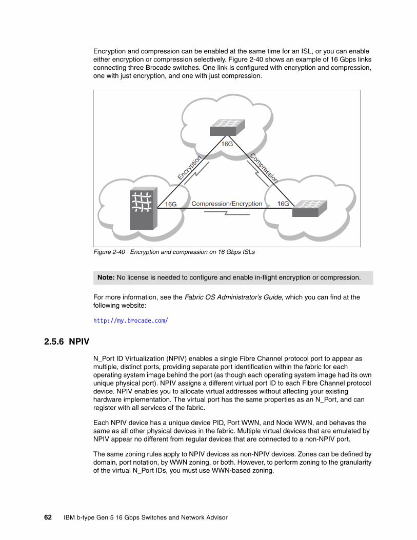
Encryption and compression can be enabled at the same time for an ISL, or you can enable either encryption or compression selectively. Figure 2-40 shows an example of 16 Gbps links connecting three Brocade switches. One link is configured with encryption and compression, one with just encryption, and one with just compression.
Figure 2-40 Encryption and compression on 16 Gbps ISLs
For more information, see the Fabric OS Administrator’s Guide, which you can find at the following website:
http://my.brocade.com/
2.5.6 NPIV
N_Port ID Virtualization (NPIV) enables a single Fibre Channel protocol port to appear as multiple, distinct ports, providing separate port identification within the fabric for each operating system image behind the port (as though each operating system image had its own unique physical port). NPIV assigns a different virtual port ID to each Fibre Channel protocol device. NPIV enables you to allocate virtual addresses without affecting your existing hardware implementation. The virtual port has the same properties as an N_Port, and can register with all services of the fabric.
Each NPIV device has a unique device PID, Port WWN, and Node WWN, and behaves the same as all other physical devices in the fabric. Multiple virtual devices that are emulated by NPIV appear no different from regular devices that are connected to a non-NPIV port.
The same zoning rules apply to NPIV devices as non-NPIV devices. Zones can be defined by domain, port notation, by WWN zoning, or both. However, to perform zoning to the granularity of the virtual N_Port IDs, you must use WWN-based zoning.
Note: No license is needed to configure and enable in-flight encryption or compression.
62 IBM b-type Gen 5 16 Gbps Switches and Network Advisor
If you are using domain port zoning for an NPIV port, and all the virtual PIDs that are associated with the port are included in the zone, then a port login (PLOGI) to a non-existent virtual PID is not blocked by the switch; rather, it is delivered to the device that is attached to the NPIV port. In cases where the device cannot handle such unexpected PLOGIs, use WWN-based zoning.
For more information, see the Fabric OS Administrator’s Guide, which you can find at the following website:
http://my.brocade.com/
2.5.7 Dynamic Fabric Provisioning
Introduced in FOS V7.0, Dynamic Fabric Provisioning (DFP) simplifies server deployment in a Fibre Channel SAN (FC SAN) environment.
Server deployment typically requires that multiple administrative teams (for example, server and storage teams) coordinate with each other to perform configuration tasks, such as zone creation in the fabric and LUN mapping and masking on the storage device. These tasks must be complete before the server is deployed. Before you can configure WWN zones and LUN masks, you must discover the physical port worldwide name (PWWN) of the server. This means that administrative teams cannot start their configuration tasks until the physical server arrives (and its physical PWWN is known). Because the configuration tasks are sequential and interdependent across various administrative teams, it might take several days before the server is deployed in an FC SAN.
DFP simplifies and accelerates new server deployment and improves operational efficiency by using a fabric-assigned PWWN (FA-PWWN). An FA-PWWN is a “virtual” port WWN that can be used instead of the physical PWWN to create zoning and LUN mapping and masking. When the server is later attached to the SAN, the FA-PWWN is then assigned to the server.
The FA-PWWN feature allows you to perform the following tasks:
� Replace one server with another server, or replace failed HBAs or adapters within a server, without having to change any zoning or LUN mapping and masking configurations.
� Easily move servers across ports or Access Gateways by reassigning the FA-PWWN to another port.
� Use the FA-PWWN to represent a server in boot LUN zone configurations so that any physical server that is mapped to this FA-PWWN can boot from that LUN, thus simplifying boot over SAN configuration.
For more information, see the Fabric OS Administrator’s Guide, which you can find at the following website:
http://my.brocade.com/
Note: For the server to use the FA-PWWN feature, it must be using a Brocade HBA or adapter. For more information, see the release notes for the HBA or adapter versions that support this feature.
Configuration of the HBA must be performed to use the FA-PWWN.
Chapter 2. Product hardware and features 63

64 IBM b-type Gen 5 16 Gbps Switches and Network Advisor

Chapter 3. IBM Network Advisor
This chapter provides initial guidance about selecting the upgrade code path for IBM Network Advisor, upgrading an existing installation of IBM Network Advisor, and installing IBM Network Advisor. It also describes the creation, addition, and deletion of user accounts, and new features that were introduced with IBM Network Advisor V12.0.3.
3
© Copyright IBM Corp. 2014. All rights reserved. 65
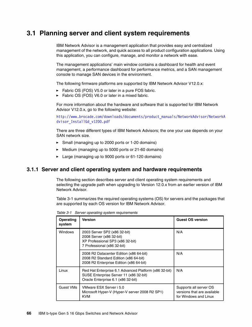
3.1 Planning server and client system requirements
IBM Network Advisor is a management application that provides easy and centralized management of the network, and quick access to all product configuration applications. Using this application, you can configure, manage, and monitor a network with ease.
The management applications’ main window contains a dashboard for health and event management, a performance dashboard for performance metrics, and a SAN management console to manage SAN devices in the environment.
The following firmware platforms are supported by IBM Network Advisor V12.0.x:
� Fabric OS (FOS) V5.0 or later in a pure FOS fabric.� Fabric OS (FOS) V6.0 or later in a mixed fabric.
For more information about the hardware and software that is supported for IBM Network Advisor V12.0.x, go to the following website:
http://www.brocade.com/downloads/documents/product_manuals/NetworkAdvisor/NetworkAdvisor_InstallGd_v1200.pdf
There are three different types of IBM Network Advisors; the one your use depends on your SAN network size.
� Small (managing up to 2000 ports or 1-20 domains)
� Medium (managing up to 5000 ports or 21-60 domains)
� Large (managing up to 9000 ports or 61-120 domains)
3.1.1 Server and client operating system and hardware requirements
The following section describes server and client operating system requirements and selecting the upgrade path when upgrading to Version 12.0.x from an earlier version of IBM Network Advisor.
Table 3-1 summarizes the required operating systems (OS) for servers and the packages that are supported by each OS version for IBM Network Advisor.
Table 3-1 Server operating system requirements
Operating system
Version Guest OS version
Windows 2003 Server SP2 (x86 32-bit)2008 Server (x86 32-bit)XP Professional SP3 (x86 32-bit)7 Professional (x86 32-bit)
N/A
2008 R2 Datacenter Edition (x86 64-bit)2008 R2 Standard Edition (x86 64-bit)2008 R2 Enterprise Edition (x86 64-bit)
N/A
Linux Red Hat Enterprise 6.1 Advanced Platform (x86 32-bit)SUSE Enterprise Server 11 (x86 32-bit)Oracle Enterprise 6.1 (x86 32-bit)
N/A
Guest VMs VMware ESX Server i 5.0Microsoft Hyper-V (Hyper-V server 2008 R2 SP1)KVM
Supports all server OS versions that are available for Windows and Linux
66 IBM b-type Gen 5 16 Gbps Switches and Network Advisor

Table 3-2 summarizes the client operating system requirements for IBM Network Advisor.
Table 3-2 Client operating system requirements
Table 3-3 summarizes the minimum host requirements for running IBM Network Advisor on Windows and Linux.
Table 3-3 Host requirements for IBM Network Advisor
Table 3-4 summarizes the minimum memory requirements for IBM Network Advisor.
Table 3-4 Memory requirements
Note: Large installations are supported on only the 64-bit Windows operating system.
Operating system
Version Guest OS version
Windows 2003 Server SP2 (x86 32-bit)2008 Server (x86 32-bit)XP Professional SP3 (x86 32-bit)7 Professional (x86 32-bit)
N/A
Linux Red Hat Enterprise 6.1 Advanced Platform (x86 32-bit/64-bit)SUSE Enterprise Server 11 (x86 32-bit)Oracle Enterprise 6.1 (x86 32-bit)
N/A
Guest VMs VMware ESX Server i 5.0Microsoft Hyper-V (Hyper-V Server 2008 R2 SP1)KVM
Supports all client OS versions that are available for Windows and Linux
Configuration Professional Professional Plus
Small Medium Large
Server plus one local client
Intel Core2 duo 2 GHz or equivalent
Intel Core2 duo 2 GHz or equivalent
Intel Core2 duo 2 GHz or equivalent
Intel Dual CPUCore2 duo 2.4 GHz or equivalent
Intel Dual CPUCore2 duo 2.4 GHz or equivalent
Remote client only
N/A Intel Core2 duo 2 GHz or equivalent
Intel Core2 duo 2 GHz or equivalent
Intel Core2 duo 2 GHz or equivalent
Intel Core2 duo 2 GHz or equivalent
Server/Client Professional Professional Plus
Small Medium Large
Server plus one local client
2 GB (32-bit)3 GB (64-bit)
3 GB (32-bit)4 GB (64-bit)
3 GB (32-bit)4 GB (64-bit)
4 GB (32-bit)6 GB (64-bit)
4 GB (32-bit)6 GB (64-bit)
Remote client only
N/A 1 GB 1 GB 2 GB 2 GB
Chapter 3. IBM Network Advisor 67

Table 3-5 summarizes the operating system cache requirements.
Table 3-5 Operating system cache requirements
Table 3-6 summarizes the minimum required disk space for IBM Network Advisor on Windows and Linux systems. Add an additional 40 GB of disk space for the default temporary directory.
Table 3-6 Minimum required disk space
3.1.2 Client and server system requirements
IBM Network Advisor has the following client and server system requirements:
� In the Professional edition, a single server supports a single client, which must be a local client only.
� In Professional Plus and Enterprise editions, a single server supports a maximum of 25 clients, which can be local or remote on 32-bit or 64-bit servers.
Installed physical memory (RAM) size
Windows Server 2003 SP2 and Windows XP Pro SP3
Windows Server 2008 and Windows 7 professional
Paging file size Minimum paging file size
Maximum paging file size
Minimum paging file size
Maximum paging file size
2 GB 2 GB 6 GB 1 GB 4 GB
3 GB 3 GB 9 GB 1 GB 4 GB
4 GB 4 GB 12 GB 1 GB 4 GB
Greater than 4 GB
N/A N/A 1 GB 4 GB
Server/Client Professional Professional Plus
Small Medium Large
Server plus one local client
10 GB 10 GB 20 GB 40 GB 60 GB
Remote client only N/A 1 GB 1 GB 1 GB 1 GB
Note: If you enable supportsave to run periodically or configure the IBM Network Advisor as the upload failure data capture location for monitored switches, then additional disk space is required. Each switch supportsave file is approximately 5 MB and each upload failure data capture file is approximately 500 KB. To determine the disk space requirements, multiply the frequency of scheduled supportsave commands by 5 MB and the expected upload failure data capture files by 500 KB before the planned periodic purge activity.
68 IBM b-type Gen 5 16 Gbps Switches and Network Advisor
� In Professional Plus and Enterprise editions, a single server supports a maximum of 25 clients, which can be local or remote on 64-bit servers. To support more than eight clients, you must make the following changes to your configuration:
– Increase the server memory size to 3 GB. You can configure the server memory size in the Options dialog box in the Memory Allocations window.
– Increase the PostgreSQL database shared buffers memory allocation to 1024 MB by editing the Install_Home\data\databases\postgresql.conf file.
3.1.3 Browser requirements for IBM Network Advisor
Starting IBM Network Advisor and Element Manager (Web tools) from the application are supported from the following browsers with the appropriate Java plug-in:
� Browsers– Windows Internet Explorer under Windows– Firefox under Windows or Linux
� Java plug-ins– Oracle JRE 1.7.0 update 09 for IBM Network Advisor– Oracle JRE 1.7.0 update 09 for web tools
For patch information, go to the following website:
http://www.oracle.com/technetwork/java/javase/downloads/index.html
3.1.4 Supported Fabric OS versions with IBM Network Advisor V12.0.x
Here are the FOS versions that are supported by IBM Network Advisor V12.0.x:
� Version 5.0.x, Version 5.1.x, Version 5.2.x, and Version 5.3.x� Version 6.0.x, Version 6.1.x, Version 6.2.x, Version 6.3.x, and Version v6.4.x� Version 7.0.x and Version 7.1.x
3.1.5 Recommended upgrade path and supported Fabric OS
The following upgrade paths are recommended for customers that are running with older versions of DCFM and want to upgrade to the target path release.
DCFM upgrade path to IBM Network Advisor target pathDCFM V10.4.x IBM Network Advisor V11.1.x IBM Network Advisor V12.0.x
Fabric Manager upgrade path to IBM Network Advisor target pathFabric Manager DCFM V10.3.x DCFM V10.4.x IBM Network Advisor V11.1.x IBM Network Advisor V12.0.x
Chapter 3. IBM Network Advisor 69
3.1.6 Enterprise Fabric Connectivity Manager upgrade path to IBM Network Advisor target path
� Enterprise Operating System products
– EFCM V9.7.x DCFM V10.3.x DCFM V10.4.x IBM Network Advisor V11.1.x or IBM Network Advisor V11.2.x
� FOS products
– EFCM V9.7.x DCFM V10.3.x DCFM V10.4.x IBM Network Advisor V11.1.x or IBM Network Advisor V12.0.x
IBM Network Advisor upgrade to target pathIBM Network Advisor V11.1.x, V11.2.x, or V11.3.x IBM Network Advisor V12.0.x
Supported Fabric OS� Version 5.0.x, Version 5.1.x, Version 5.2.x, and Version 5.3.x� Version 6.0.x, Version 6.1.x, Version 6.2.x, Version 6.3.x, and Version v6.4.x� Version 7.0.x and Version 7.1.x
3.1.7 Downloading software
You can download the software and documentation from the MyBrocade website at the following URL:
http://my.brocade.com/
Enter your user ID and password. If you do not have a MyBrocade account, you can create one at the website.
Complete the following steps:
1. Click LOG IN.
2. Click Downloads on the main page.
3. Select Management software from the Download by list.
4. Click IBM Network Advisor in the Product Name list and select the highest version that is available.
5. Select one of the following links to download the software:
– IBM Network Advisor 12.0.3 for Windows
– IBM Network Advisor 12.0.3 for Linux
You can access the release notes and MD5 checksum from this location.
6. Read the Export Compliance, select the certification check box, and click Submit.
7. Read the Brocade End User License Agreement and click I Accept.
8. Click Save in the File Download dialog box.
9. Browse to the location where you want to save the software and click Save.
70 IBM b-type Gen 5 16 Gbps Switches and Network Advisor

3.1.8 Pre-installation requirements
Before you install IBM Network Advisor, ensure that you meet the following requirements:
� For specific system requirements, see 3.1.1, “Server and client operating system and hardware requirements” on page 66.
� To avoid errors, close all instances of the application before beginning the installation or any uninstallation procedure.
� For UNIX systems, if you still receive error message after closing the application, enter the following commands:
a. #ps -ef | grep -i “” to list the process ID
b. #kill -9 “Process_ID”, where Process_ID is any management application process
Additional pre-installation requirements for UNIX systemsEnsure that you meet the following requirements for a UNIX system:
� Ensure that an “X Server” is available for display and is configured to permit “X Client” applications to display from the host on which they are installing the IBM Network Advisor server. (Typically, this simply requires that the system console is present and running with a logged-in user on the X Server-based desktop session, such as KDE or GNOME.)
� Ensure that the DISPLAY environment variable is correctly defined in the shell with a valid value (for example, to display to the local console, run export DISPLAY=:0.0, or to display to a remote system that has an X Server running, run export DISPLAY=Remote_IP_address:0.0). You might also need to configure your firewall because it might block the display to the X Server, which listens by default on TCP port 6000 on the remote host.
� To display to a remote system, you must permit the remote display of the X Server by running xhost+IP, where IP is the IP address of the IBM Network Advisor server host from the X-based desktop of the remote system.
� Make sure that you test the DISPLAY definition by running xterm from the same shell from which you run install.bin. A new X terminal window to the destination X Server display should open.
� For Linux OS with the SELinux security policy enabled, ensure that you complete the following steps:
a. Disable the SELinux security policy by running setenforce 0/.
b. Install the application, as described in 3.2.1, “New installation of IBM Network Advisor” on page 73.
c. Enable the SELinux security policy by running setenforce 1.
Mapping a loopback address to the local hostTo map the loopback address to the local host, complete the following steps.
1. Open the host file.
– For Windows, the hosts file is in the WINDOWS\system32\drivers\etc directory.
– For Linux, the host file is in the /etc directory.
Chapter 3. IBM Network Advisor 71
2. Add the following entries:
– For an IPV4 machine
127.0.0.1 localhost
– For an IPV6 machine
127.0.0.1 localhost::1 localhost
3. Save and close the file.
3.1.9 Syslog troubleshooting
If the default syslog port number is in use, you do not receive any syslog messages from the device. Use one of the following procedures (depending on your operating system) to determine which process is running on the syslog port and to stop the process.
Finding the processTo find the process, complete the following steps:
1. Open a command window.
2. Choose one of the following options:
– On Linux systems, enter netstat -nap | grep 514 and press Enter.
• The process running on port 514 displays.
• Example output: UDP 0 0 ::ffff:127:0:0:1:514 :::* 27397
– On Windows system, enter netstat -anb | find /i “514” and press Enter.
• The process running on port 514 displays.
• Example output: UDP 127:0:0:1:514 *:* 3328
Stopping the processChoose one of the following options:
� On Linux systems, enter Kill -9 “<PID>” and press Enter. For example, kill -9 “27397”.
� On Windows systems, enter taskkill /F /PID “<PID>” and press Enter. For example, taskkill /F /PID “3328”. You can also run the following procedure instead for Windows:
a. Press Ctrl+Shift+Esc to open the Windows Task Manager.b. Click the Processes tab.c. Click the PID column header to sort the processes by PID.d. Select the process that you want to stop and click End Process.
3.2 New installations and upgrading IBM Network Advisor to Version 12.0.3
Before you install the application, ensure that your system meets the minimum pre-installation requirements that are described in 3.1.8, “Pre-installation requirements” on page 71. If you are migrating data (upgrading), see 3.2.2, “Upgrading to IBM Network Advisor V12.0.x from an existing IBM Network Advisor installation” on page 93.
72 IBM b-type Gen 5 16 Gbps Switches and Network Advisor
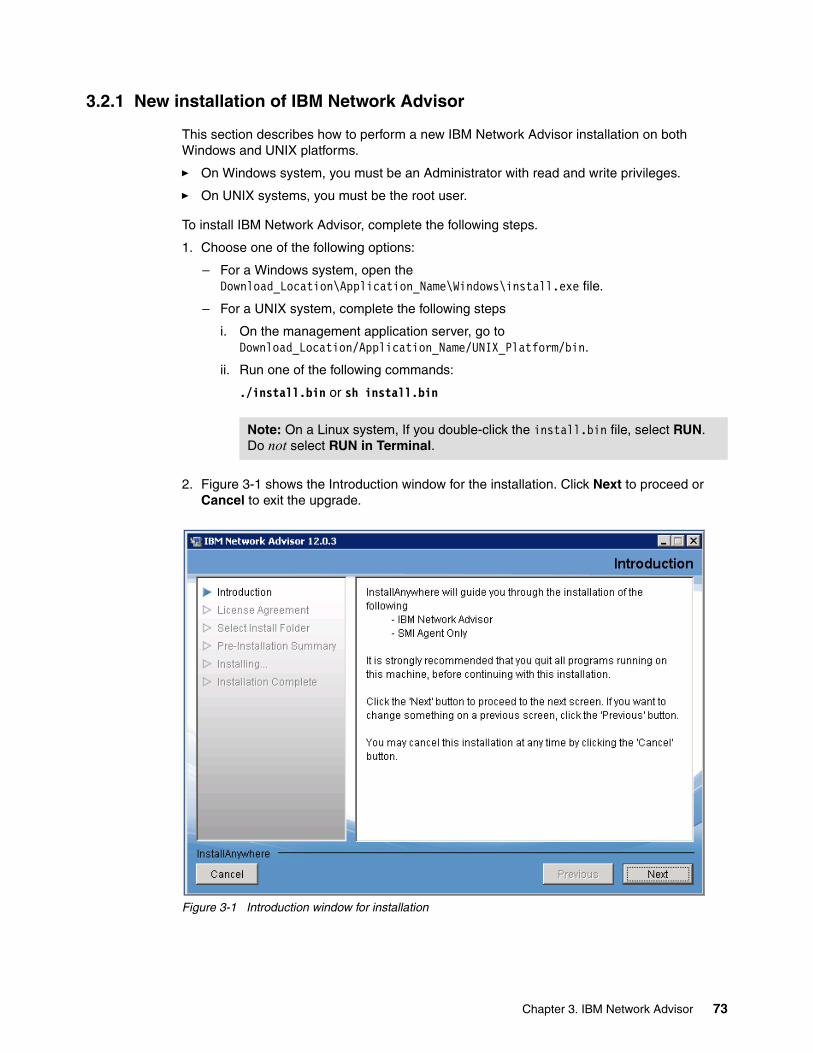
3.2.1 New installation of IBM Network Advisor
This section describes how to perform a new IBM Network Advisor installation on both Windows and UNIX platforms.
� On Windows system, you must be an Administrator with read and write privileges.
� On UNIX systems, you must be the root user.
To install IBM Network Advisor, complete the following steps.
1. Choose one of the following options:
– For a Windows system, open the Download_Location\Application_Name\Windows\install.exe file.
– For a UNIX system, complete the following steps
i. On the management application server, go to Download_Location/Application_Name/UNIX_Platform/bin.
ii. Run one of the following commands:
./install.bin or sh install.bin
2. Figure 3-1 shows the Introduction window for the installation. Click Next to proceed or Cancel to exit the upgrade.
Figure 3-1 Introduction window for installation
Note: On a Linux system, If you double-click the install.bin file, select RUN. Do not select RUN in Terminal.
Chapter 3. IBM Network Advisor 73

3. A window with the license agreement opens. Accept the IBM Network Advisor license to proceed. After you accept the license agreement, you are prompted for the installation location. Do not install to the root directory (C:\Windows or / (UNIX)).
Figure 3-2 shows the options to choose the installation location.
Figure 3-2 Installation folder options
74 IBM b-type Gen 5 16 Gbps Switches and Network Advisor
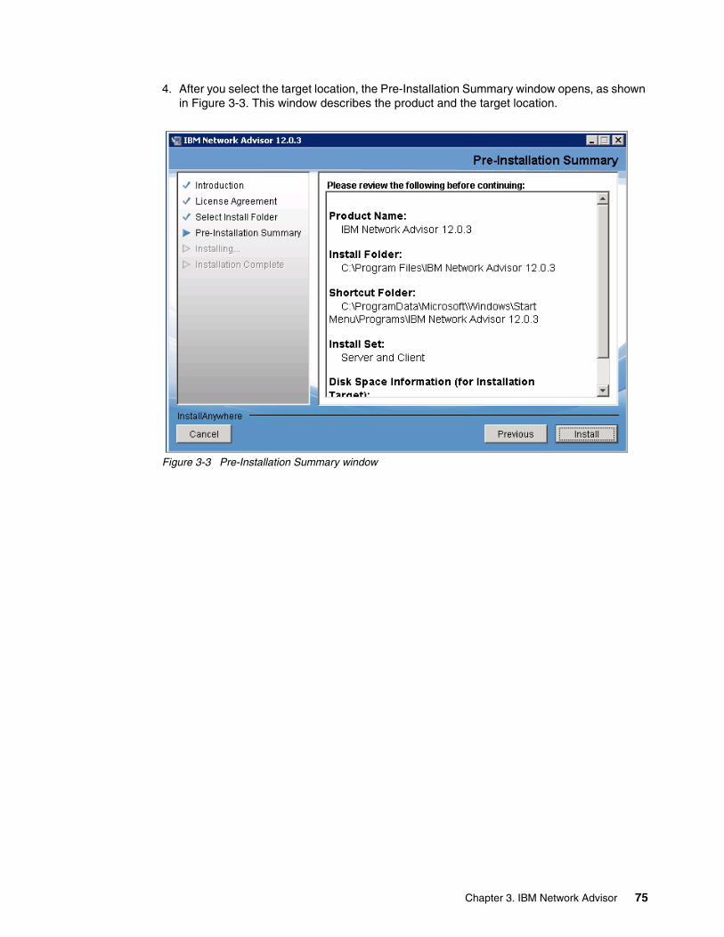
4. After you select the target location, the Pre-Installation Summary window opens, as shown in Figure 3-3. This window describes the product and the target location.
Figure 3-3 Pre-Installation Summary window
Chapter 3. IBM Network Advisor 75
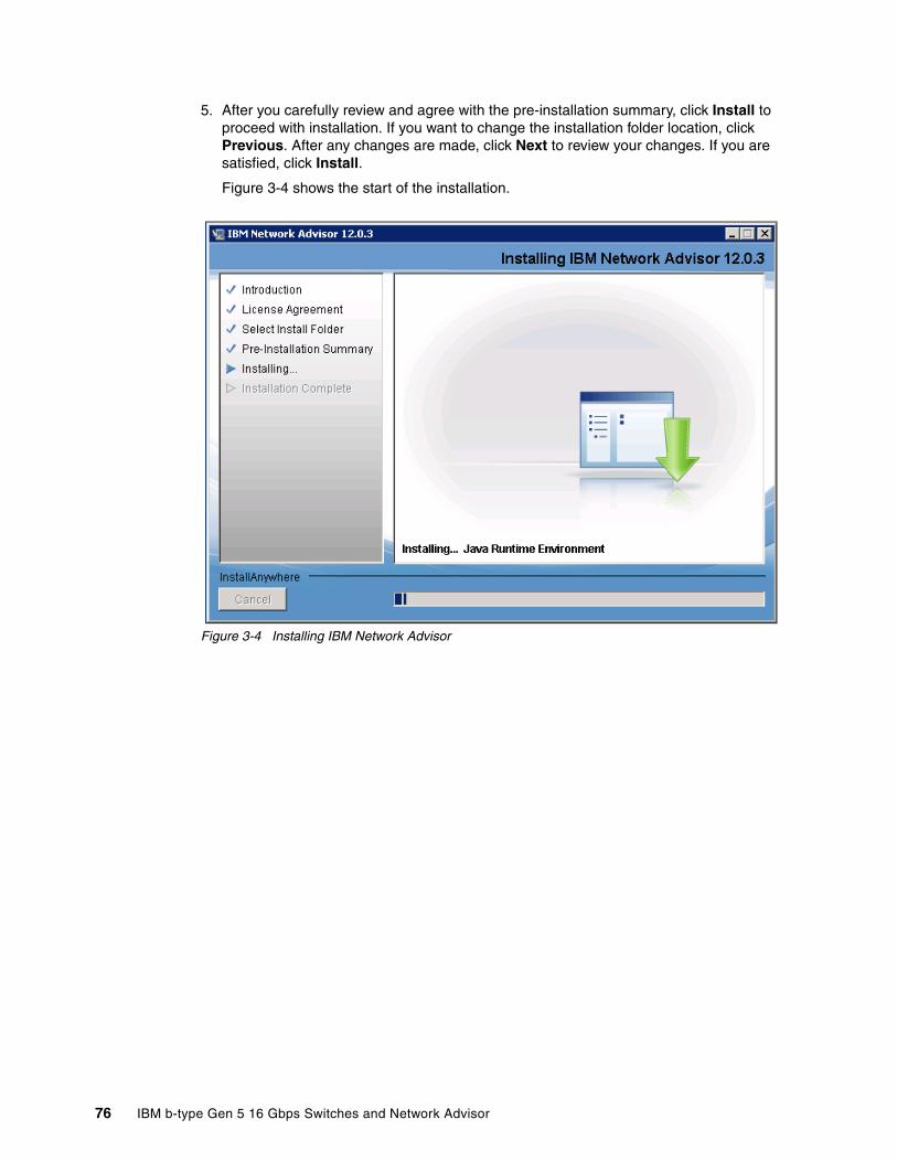
5. After you carefully review and agree with the pre-installation summary, click Install to proceed with installation. If you want to change the installation folder location, click Previous. After any changes are made, click Next to review your changes. If you are satisfied, click Install.
Figure 3-4 shows the start of the installation.
Figure 3-4 Installing IBM Network Advisor
76 IBM b-type Gen 5 16 Gbps Switches and Network Advisor

6. After the completion of the installation, as shown in Figure 3-5, the Installation Complete window opens. Ensure that the Launch IBM Network Advisor Configuration check box is selected to proceed with the configuration (it is selected by default). Click Done.
Figure 3-5 Installation Complete window
If the local host is not mapped to the loopback address, an error message displays, so you must map the loopback address to the local host. To learn how to configure the loopback address, see “Mapping a loopback address to the local host” on page 71.
Chapter 3. IBM Network Advisor 77

If the “Launch IBM Network Advisor Configuration” box is cleared, as shown in Figure 3-6, a dialog box opens that prompts you to select the box.
Figure 3-6 Alert window for configuration check box
78 IBM b-type Gen 5 16 Gbps Switches and Network Advisor

7. After you select the check box and click Done, the Welcome window opens and describes migrating data and settings, choosing the installation type, license, FTP server, ports, server IP SMI agent, and network size, as shown in Figure 3-7. Click Next.
Figure 3-7 Welcome window
Chapter 3. IBM Network Advisor 79

8. The Copy Data and Settings from previous releases window opens and prompts you for a copy of the data and settings from your previous installation. As this is a new installation, select No, don’t copy any data and settings, as shown in Figure 3-8. Click Next.
Figure 3-8 Copy Data and Settings from previous releases window
80 IBM b-type Gen 5 16 Gbps Switches and Network Advisor
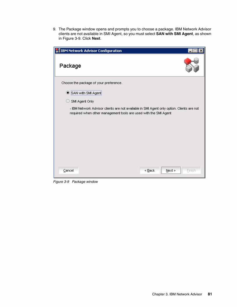
9. The Package window opens and prompts you to choose a package. IBM Network Advisor clients are not available in SMI Agent, so you must select SAN with SMI Agent, as shown in Figure 3-9. Click Next.
Figure 3-9 Package window
Chapter 3. IBM Network Advisor 81

10.The Installation Type window opens and prompts you to choose an installation type, as shown in Figure 3-10.
Figure 3-10 Choosing the installation type
There are two options: Licensed version and 75 days trial. Select IBM Network Advisor - Licensed version and click Next.
Note: Obtain and store the license in a known secure location before proceeding with the upgrade.
82 IBM b-type Gen 5 16 Gbps Switches and Network Advisor

11.The Server License window opens and prompts you to enter the license details, as shown Figure 3-11. Input the serial number and license key by clicking Browse and navigating to the location of the file that contains the information. Click Next.
Figure 3-11 Providing license details
Chapter 3. IBM Network Advisor 83

12.The FTP / SCP / SFTP Server window opens and prompts you to configure the FTP server, as shown in Figure 3-12.
Figure 3-12 Choosing an FTP server
This window shows the options of Built-in FTP/SCP/SFTP server and External FTP/SCP/SFTP server. The server where IBM Network Advisor is installed also behaves as an FTP server, so it is a preferred practice to choose the Built-in FTP/SCP/SFTP option. If you choose External FTP/SCP/SFTP, ensure that the server where the IBM Network Advisor is installed is also configured as an FTP server because if you do not do so, the Firmware repository feature will not be available.
Select the Built-in FTP/SCP/SFTP option and click Next.
84 IBM b-type Gen 5 16 Gbps Switches and Network Advisor
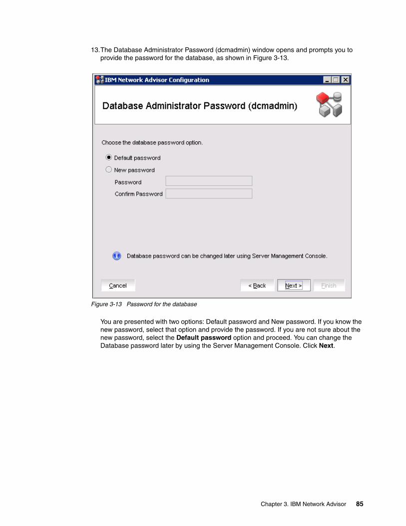
13.The Database Administrator Password (dcmadmin) window opens and prompts you to provide the password for the database, as shown in Figure 3-13.
Figure 3-13 Password for the database
You are presented with two options: Default password and New password. If you know the new password, select that option and provide the password. If you are not sure about the new password, select the Default password option and proceed. You can change the Database password later by using the Server Management Console. Click Next.
Chapter 3. IBM Network Advisor 85

14.The Server IP Configuration window opens and prompts you to enter the server IP configuration details, as shown in Figure 3-14. In the Server IP Configuration drop-down box, you can choose a server name only if DNS is configured in the environment. If DNS is not configured, choose the IP address. Click Next.
Figure 3-14 Server IP Configuration details
86 IBM b-type Gen 5 16 Gbps Switches and Network Advisor

15.The Server Configuration window opens and prompts you to provide the port details, as shown in Figure 3-15.
Figure 3-15 Port details
Complete the following steps:
a. Enter a port number in the Web Server Port# (HTTPS) field (the default is 443).
• Enable HTTP redirection to HTTPS by selecting the Redirect HTTP Requests to HTTPS check box.
• When you enable HTTP redirection, the server uses port 80 to redirect HTTP requests to HTTPS. You can configure the server port settings by using the Options dialog box in the Server Port pane.
b. Enter a port number in the Database Port# field (Default is 5432). Do not use a port number below 1024.
c. Enter a port number in the Starting Port Number field (the default is 24600).
• For Professional software, the server requires 15 consecutive free ports beginning with the starting port number.
• For Trial and Licensed software, the server requires 18 consecutive free ports beginning with the starting port number.
d. Enter a port number in the Syslog Port Number field (the default is 514). If the default Syslog port is already in use, you do not receive any syslog messages from the device. To find and stop the process that is running on the default Syslog port number, see 3.1.9, “Syslog troubleshooting” on page 72.
Chapter 3. IBM Network Advisor 87

e. Enter a port number in the SNMP Port Number field (the default is 162).
Click Next to proceed with the installation. If you enter a syslog port number that is already in use, a message is displayed. Click No to remain in the Server Configuration window and edit the syslog port number. Click Yes to close the message.
If you enter a port number that is already in use, a warning displays next to the associated port number field. Edit that port number and click Next.
16.The SMI Agent Configuration window opens and prompts you to configure the SMI Agent, as shown in Figure 3-16.
Figure 3-16 SMI Agent Configuration window
Select the Enable SSL check box and enter 5989 as the port number (the default is 5988). Click Next.
88 IBM b-type Gen 5 16 Gbps Switches and Network Advisor

17.The SAN Network Size window opens and prompts you to configure the SAN network, as shown in Figure 3-17. Choose the option that best suits your network size and click Next.
Figure 3-17 SAN Network Size window
Chapter 3. IBM Network Advisor 89

18.The Server Configuration Summary window opens, as shown in Figure 3-18. Review the details in the window; if you are satisfied, click Next.
Figure 3-18 Server Configuration Summary window
90 IBM b-type Gen 5 16 Gbps Switches and Network Advisor

19.The Start Serve window opens and prompts you to start the server and client, as shown in Figure 3-19. You can start the client after the installation by selecting the Start Client check box, or you can leave it clear to start the client at a later stage.
Figure 3-19 Starting the server and client
Ensure that the Service window (under Administrative Tools) is closed. If the Services window is open, IBM Network Advisor might fail to start.
Select Finish.
Chapter 3. IBM Network Advisor 91
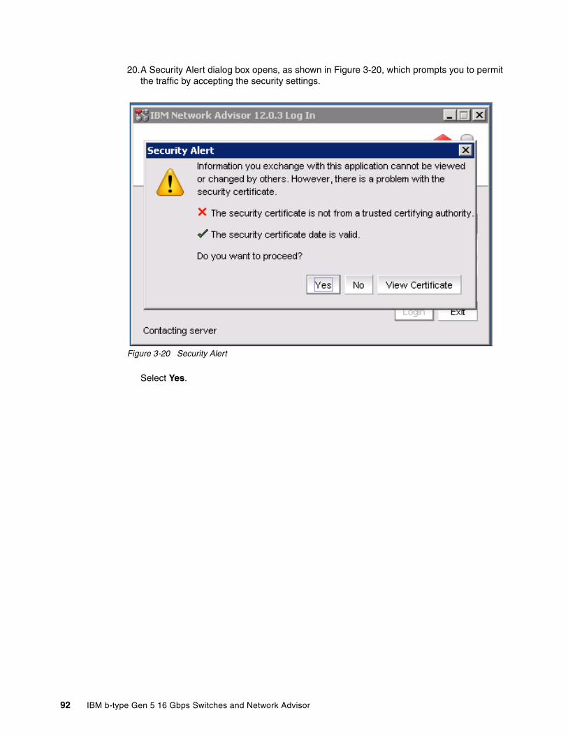
20.A Security Alert dialog box opens, as shown in Figure 3-20, which prompts you to permit the traffic by accepting the security settings.
Figure 3-20 Security Alert
Select Yes.
92 IBM b-type Gen 5 16 Gbps Switches and Network Advisor

21.A login window opens and prompts you to provide the logIn credentials, as shown in Figure 3-21. The default credentials are administrator/password. After you provide the credentials, click Login.
Figure 3-21 LogIn window
3.2.2 Upgrading to IBM Network Advisor V12.0.x from an existing IBM Network Advisor installation
This section describes upgrading an existing IBM Network Advisor installation to Version 12.0.x. For the upgrade path reference, see 3.1.5, “Recommended upgrade path and supported Fabric OS” on page 69. During the upgrade process, the old version is uninstalled and the new version with an upgraded database is installed.
Before you proceed with the upgrade, back up your configuration. To back up your configuration, go to installation location and copy the IBM Network Advisor 12.0.x folder.
This section describes upgrading to IBM Network Advisor V12.0.x on both Windows and UNIX platforms:
� On Windows system, you must be an administrator with read and write privileges.
� On UNIX systems, you must be the root user.
Chapter 3. IBM Network Advisor 93

To upgrade the new application version, complete the following steps.
1. Choose one of the following options:
– For a Windows system, open the Download_Location\Application_Name\Windows\install.exe file.
– For a UNIX system, complete the following steps:
i. On the management application server, go to the Download_Location/Application_Name/UNIX_Platform/bin directory.
ii. Run one of the following commands:
./install.bin or sh install.bin
2. The Introduction window opens, as shown in Figure 3-1 on page 73. Click Next to proceed or Cancel to exit the upgrade.
3. A window with the license agreement opens. Accept the license agreement to proceed to the next step. A window opens and prompts you for the installation folder location, As shown in Figure 3-2 on page 74. Select the default location, as it is the current IBM Network Advisor installed folder location. If you want to choose a different location, do so now. Click Next.
4. The Pre-Installation Summary window opens, as shown in Figure 3-3 on page 75. Select Install to proceed with the installation.
5. After the installation completes, the Installation Complete window opens, as shown in Figure 3-5 on page 77. Select the Launch IBM Network Advisor Configuration check box and click Done to start the configuration.
6. The Welcome window opens and describes the migrate data and settings, choosing the installation type, license, FTP server, ports, server IP SMI agent, and network size, as shown in Figure 3-7 on page 79. Click Next.
7. The Copy Data and Settings from previous releases window opens and prompts you for a copy of the data and settings from your previous installation, as shown in Figure 3-22 on page 95. You must provide the folder location where the previous version was installed. It is not possible to migrate the data from a previous version after the installation.
Note: On a Linux system, if you double-click the install.bin file, select RUN. Do not select RUN in Terminal.
94 IBM b-type Gen 5 16 Gbps Switches and Network Advisor
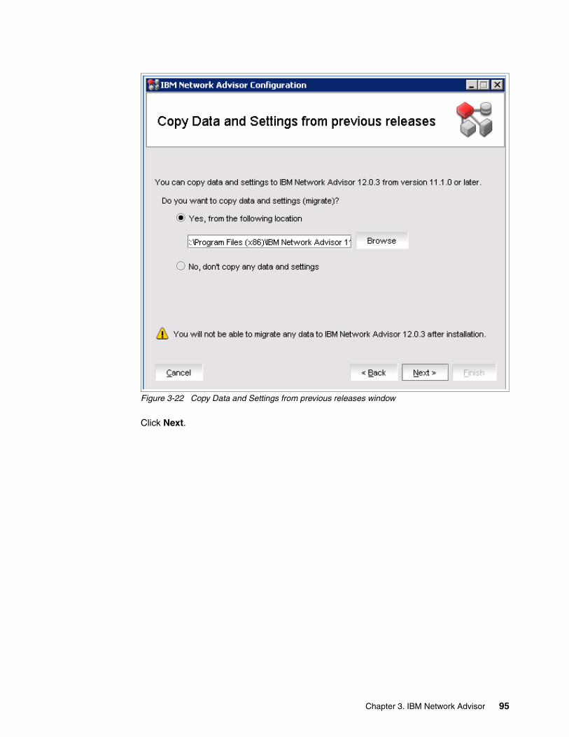
Figure 3-22 Copy Data and Settings from previous releases window
Click Next.
Chapter 3. IBM Network Advisor 95

8. A dialog box with information about Call Home settings opens, as shown in Figure 3-23. This feature is introduced with IBM Network Advisor V12.0.3, where products that are associated with Brocade North America and Brocade International Call Home centers are mapped to the Brocade email Call Home call center after the migration. You may select Yes, No, or Cancel, and then click Next.
Figure 3-23 Window with Call Home settings
96 IBM b-type Gen 5 16 Gbps Switches and Network Advisor
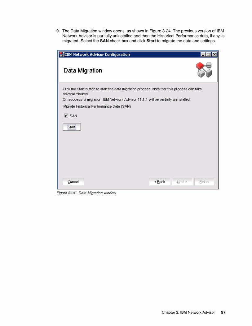
9. The Data Migration window opens, as shown in Figure 3-24. The previous version of IBM Network Advisor is partially uninstalled and then the Historical Performance data, if any, is migrated. Select the SAN check box and click Start to migrate the data and settings.
Figure 3-24 Data Migration window
Chapter 3. IBM Network Advisor 97
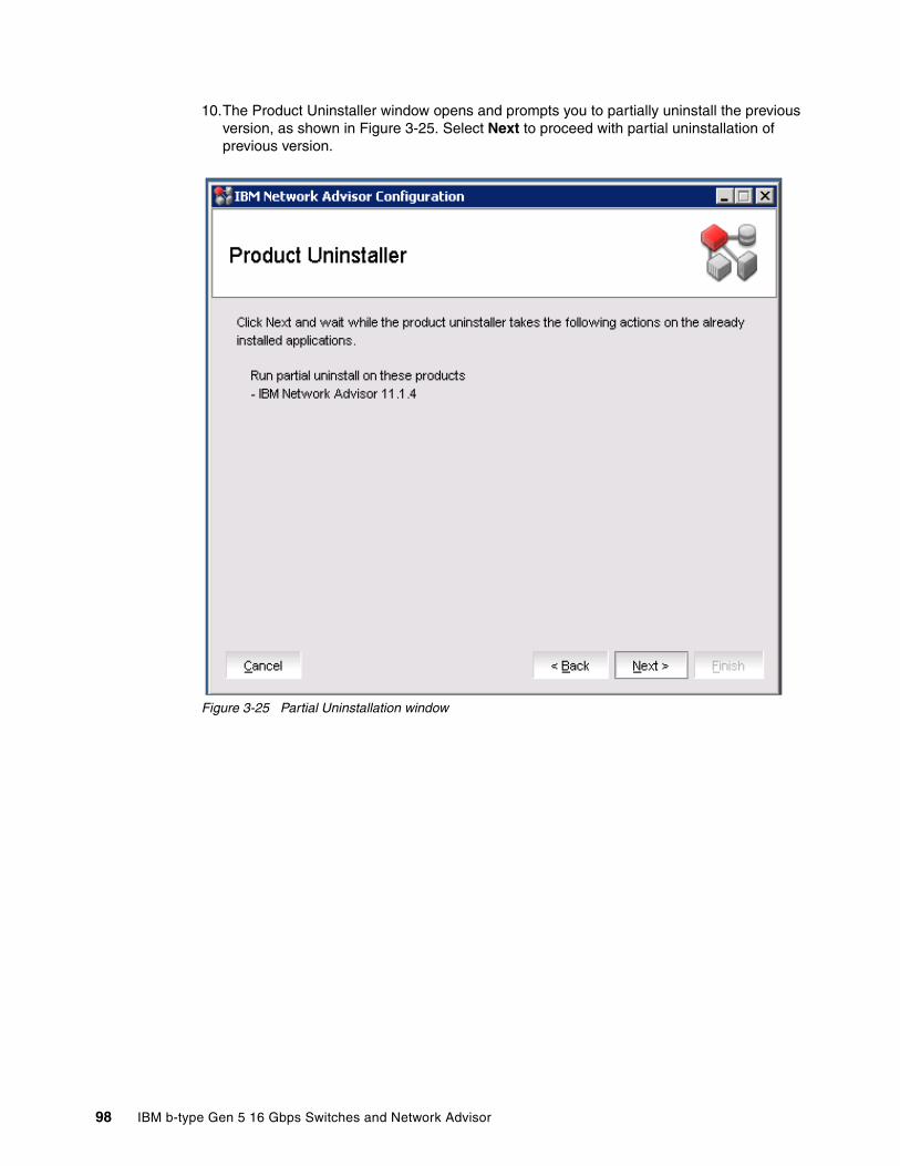
10.The Product Uninstaller window opens and prompts you to partially uninstall the previous version, as shown in Figure 3-25. Select Next to proceed with partial uninstallation of previous version.
Figure 3-25 Partial Uninstallation window
98 IBM b-type Gen 5 16 Gbps Switches and Network Advisor

After the successful partial uninstallation, the window that is shown in Figure 3-26 opens and shows the migration of the historical data from the previous version.
Figure 3-26 Migrating Database
Chapter 3. IBM Network Advisor 99
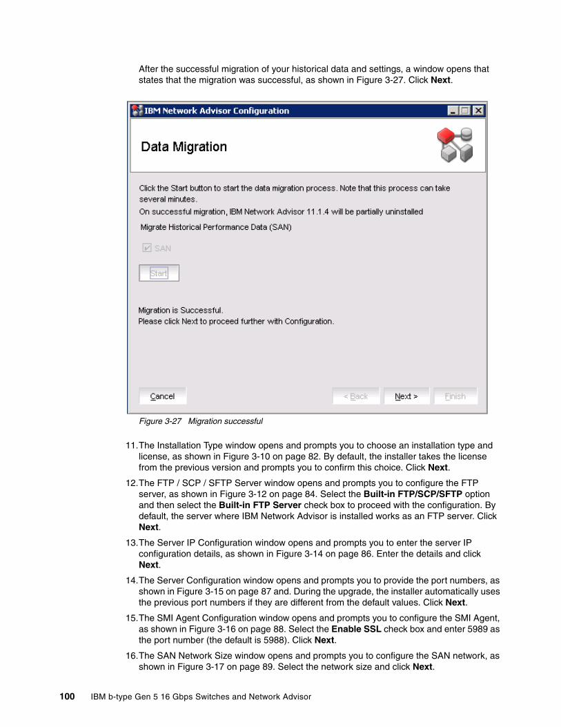
After the successful migration of your historical data and settings, a window opens that states that the migration was successful, as shown in Figure 3-27. Click Next.
Figure 3-27 Migration successful
11.The Installation Type window opens and prompts you to choose an installation type and license, as shown in Figure 3-10 on page 82. By default, the installer takes the license from the previous version and prompts you to confirm this choice. Click Next.
12.The FTP / SCP / SFTP Server window opens and prompts you to configure the FTP server, as shown in Figure 3-12 on page 84. Select the Built-in FTP/SCP/SFTP option and then select the Built-in FTP Server check box to proceed with the configuration. By default, the server where IBM Network Advisor is installed works as an FTP server. Click Next.
13.The Server IP Configuration window opens and prompts you to enter the server IP configuration details, as shown in Figure 3-14 on page 86. Enter the details and click Next.
14.The Server Configuration window opens and prompts you to provide the port numbers, as shown in Figure 3-15 on page 87 and. During the upgrade, the installer automatically uses the previous port numbers if they are different from the default values. Click Next.
15.The SMI Agent Configuration window opens and prompts you to configure the SMI Agent, as shown in Figure 3-16 on page 88. Select the Enable SSL check box and enter 5989 as the port number (the default is 5988). Click Next.
16.The SAN Network Size window opens and prompts you to configure the SAN network, as shown in Figure 3-17 on page 89. Select the network size and click Next.
100 IBM b-type Gen 5 16 Gbps Switches and Network Advisor

17.The Server Configuration Summary window opens, as shown in Figure 3-18 on page 90. If you want to change the settings, click Back and change the settings. If you do not want to change the settings, click Next.
18.The Start Serve window opens and prompts you to start the server and client, as shown in Figure 3-19 on page 91. Select the Start Client check box to start the Server and Client and click Finish.
19.A login window opens and prompts you to provide the logIn credentials, as shown in Figure 3-21 on page 93. After you provide the credentials, click Login to start using the upgraded IBM Network Advisor.
3.3 User, device, and dashboard management
The following sections describe user management and discovery, which is the process by which the management application contacts the devices in your SAN. When you configure discovery, the application discovers devices that are connected to the SAN. The application illustrates each device and its connections on the connectivity map (topology).
3.3.1 User management
User management describes how to create users, how to modify the users by adding or removing roles, and how to delete user accounts. With user management, you can control the view and management of networks by defining policies.
For more information about user management, see the following website:
http://www.brocade.com/downloads/documents/product_manuals/B_SAN/FOS_AdminGd_v701.pdf
Creating usersBy default, the “Administrator” account is created when you are installing or upgrading IBM Network Advisor. The first time you log in, use the default administrator credentials administrator (for the user ID) and password (for the password). For security reasons, change the administrator default password. To create a user, click Server Users.
Chapter 3. IBM Network Advisor 101

As shown in Figure 3-28 a window opens with the Users, Policy, and LDAP Authorization tabs. Click Users and then click Add to create a user.
In the Users tab, you can see three main panes: Users, Roles that is assigned to the user, and Area of Responsibilities (AoR). In the Users pane, you can see all the users. When you select a user, you can see their roles and responsibilities in the Roles and AoR panes.
Figure 3-28 Users tab
102 IBM b-type Gen 5 16 Gbps Switches and Network Advisor

Before you create users, define the email Event Notification, as shown in Figure 3-29 because if you do not define the email Event notification, you cannot create users.
Figure 3-29 Email Event Notification
Chapter 3. IBM Network Advisor 103

After you define the email Event Notification, click Add in the Users pane to start creating users. Provide all the details and click OK, as shown in Figure 3-30.
While you create users, you can define roles for the SAN administrators by using the Roles tab. You can assign both roles and AoR. Select the roles that you want to assign from the Available Roles / AOR pane and click the right arrow to move them to Selected Roles / AOR pane, and then click OK. For information about modifying the user, see “Modifying user accounts” on page 105.
Figure 3-30 Adding a user
104 IBM b-type Gen 5 16 Gbps Switches and Network Advisor

Modifying user accountsTo modify a user account, click Servers Users, go to the Users pane, click the account you want to modify, and select Edit. A window opens, as shown in Figure 3-31. Select the roles that you want to add / remove and click OK. You can also change the password, email address, and email notification filter.
Figure 3-31 Edit User pane
Chapter 3. IBM Network Advisor 105
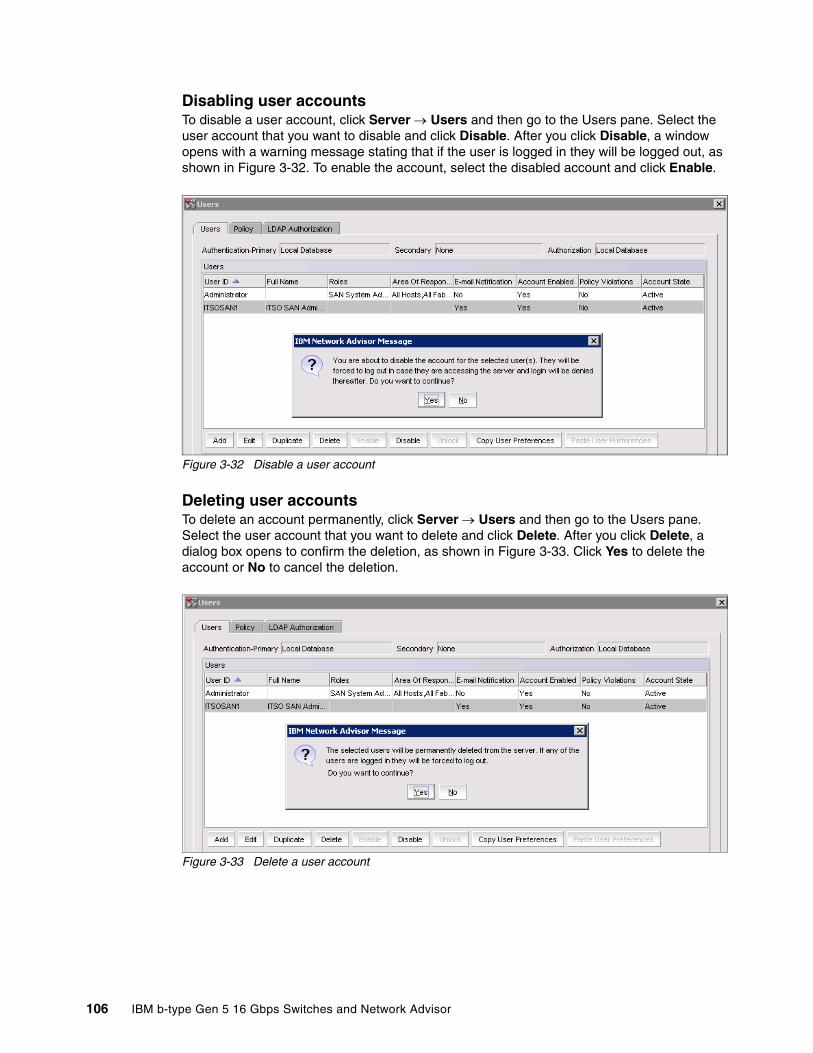
Disabling user accountsTo disable a user account, click Server Users and then go to the Users pane. Select the user account that you want to disable and click Disable. After you click Disable, a window opens with a warning message stating that if the user is logged in they will be logged out, as shown in Figure 3-32. To enable the account, select the disabled account and click Enable.
Figure 3-32 Disable a user account
Deleting user accountsTo delete an account permanently, click Server Users and then go to the Users pane. Select the user account that you want to delete and click Delete. After you click Delete, a dialog box opens to confirm the deletion, as shown in Figure 3-33. Click Yes to delete the account or No to cancel the deletion.
Figure 3-33 Delete a user account
106 IBM b-type Gen 5 16 Gbps Switches and Network Advisor

Defining policies for user accountsAs shown in Figure 3-34, you can define different policies for a user account. You can set the password age and the warning period to alert about the expiration of the current password, and the password history. Also, you can set a policy to define a password with a lockout threshold and the lockout duration. Click View Policy Violators to see any user accounts that were violated.
For more information about password policies, go to the following website:
http://www.brocade.com/downloads/documents/product_manuals/B_SAN/FOS_AdminGd_v701.pdf
Figure 3-34 Setting a policy for user accounts
Chapter 3. IBM Network Advisor 107
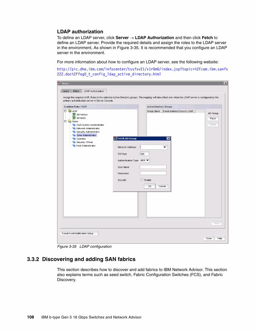
LDAP authorizationTo define an LDAP server, click Server LDAP Authorization and then click Fetch to define an LDAP server. Provide the required details and assign the roles to the LDAP server in the environment, As shown in Figure 3-35. It is recommended that you configure an LDAP server in the environment.
For more information about how to configure an LDAP server, see the following website:
http://pic.dhe.ibm.com/infocenter/tssfsv21/v1r0m0/index.jsp?topic=%2Fcom.ibm.sanfs222.doc%2Ffog0_t_config_ldap_active_directory.html
Figure 3-35 LDAP configuration
3.3.2 Discovering and adding SAN fabrics
This section describes how to discover and add fabrics to IBM Network Advisor. This section also explains terms such as seed switch, Fabric Configuration Switches (FCS), and Fabric Discovery.
108 IBM b-type Gen 5 16 Gbps Switches and Network Advisor

Seed switch (discovery switch)The discovery switch is a switch in the fabric that uses in-band communication to obtain fabric-wide information about the name server, zoning, and fabric membership from all other switches. There must be at least one discovery switch present in all fabrics. The presence of a discovery switch provides significant help in improving the scalability of the application.
In this section, the discovery switch is also referred to as a seed switch.
The seed switch must be running a supported FOS and must be HTTP reachable. Sometimes, the seed switch is auto-selected, such as when a fabric segments or when two fabrics merge. Other times, you are prompted (when an event is triggered) to change the seed switch, such as in the following cases:
� If during a fabric discovery the management application detects that the seed switch is not running a supported version, you are prompted to change the seed switch.
� When one or more switches join the fabric or if the switch firmware is changed on any of the switches in the fabric, the management application checks to make sure that the seed switch is still running a supported version. If it is not, then you are prompted to either upgrade the firmware on the seed switch or to change the seed switch to a switch running supported firmware.
If a fabric of switches running only FOS V5.X or later is created because of segmentation, the management application continues to monitor that fabric, but if any switch with a later FOS version joins the fabric, an event is triggered and informs you that the seed switch is not running the latest firmware and you should change to a seed switch that is running the highest level of firmware.
You can change the seed switch if the following conditions are met:
� The new seed switch is HTTP-reachable from the management application.� The new seed switch is a primary FCS.� The new seed switch is running the latest FOS version in the fabric.
This operation preserves historical and configuration data, such as performance monitoring and user-customized data for the selected fabric.
If during the seed switch change the fabric is deleted but the rediscovery operation fails (for example, if the new seed switch becomes unreachable using HTTP), then you must rediscover the fabric again. If you rediscover the fabric by using a switch that was present in the fabric before the change seed switch operation was performed, then all of the historical and configuration data is restored to the rediscovered fabric. If you rediscover the fabric by using a switch that was added to the fabric after the fabric was deleted, then the historical and configuration data is lost.
If multiple users try to change the seed switch of the same fabric simultaneously, only the first change seed switch request is run; subsequent requests that are initiated before the first request completes fail.
Note: If a seed switch is segmented or merged, historical data, such as the offline zone database, profile, reports, and Firmware Download profile, can be lost. Segmentation of a seed switch does not result in formation of a new fabric. If a merge occurs, the historical data is lost only from the second fabric.
Note: If the seed switch firmware is downgraded from FOS V5.2.X to an earlier version, then all RBAC-related data is discarded from the management application.
Chapter 3. IBM Network Advisor 109

If another user changes the seed switch of a fabric you are monitoring, and if you have provided login credentials for only that seed switch in the fabric, then you lose connection to that seed switch.
Seed switch failoverThe management application collects fabric-wide data (such as fabric membership, connectivity, name server information, and zoning) by using the seed switch. Therefore, when a seed switch becomes unreachable or there is no valid seed switch, the fabric becomes unmanageable.
When the seed switch cannot be reached for three consecutive fabric refresh cycles, the management application looks for another valid seed switch in the fabric, verifies that it can be reached, and has valid credentials. If the seed switch meets this criteria, the management application automatically fails over to the recommended seed switch.
It is possible that auto-failover might occur to a seed switch that is not running the latest firmware version. In this instance, any function that has a direct dependency on the firmware version of the seed switch is affected and restricted by the failover seed switch capabilities.
Changing the seed switchWhen you change the seed switch for a fabric, the management application performs the following checks in the following order:
� Identifies all switches and removes those switches running unsupported firmware versions.
� Identifies which of the remaining switches are running the latest firmware versions.
� Filters out those switches that are not reachable.
� Identifies which switches are Virtual Fabric-enabled switches (FOS only). If there are Virtual Fabric-enabled switches, the management application uses only these switches as recommended seed switches. If there are no Virtual Fabric-enabled switches, it continues with the next check.
� Identifies which switches are Virtual Fabric-capable devices (FOS only). If there are Virtual Fabric-capable switches, the management application uses only these switches as recommended seed switches. If there are no Virtual Fabric-capable switches, the management application uses the list from the second check.
To change the seed switch, complete the following steps.
1. Click Discovery Fabrics. The Discover Fabrics dialog box opens.
2. Select the fabric for which you want to change the seed switch from the Discovered Fabrics table.
If a device joins or merges with a fabric and fabric tracking is active, you must accept changes to the fabric before the new devices display in the Seed Switch dialog box. For more information about fabric tracking, see the following website:
ftp://index.storsys.ibm.com/san/brcd/na-user-guide-v11.1.pdf
3. Click Seed Switch.
If the fabric contains other switches that are running the latest version and are also HTTP-reachable from the management application, the Seed Switch dialog box opens. Otherwise, a message displays that you cannot change the seed switch.
4. Select a switch to be the new seed switch from the Seed Switch dialog box.
110 IBM b-type Gen 5 16 Gbps Switches and Network Advisor

You can select only one switch. Only switches that are running the latest FOS version in the fabric are displayed. The current seed switch is not displayed in this list.
5. Click OK in the Seed Switch dialog box.
If you are not already logged in to the seed switch, the Fabric Login dialog box opens.
If you are successfully authenticated, the fabric is deleted from the management application without purging historical data, and the same fabric is rediscovered with the new seed switch.
6. Click Close in the Discover Fabrics dialog box.
Fabric Configuration Server policiesThe Fabric Configuration Server (FCS) policy in the base FOS may be set on a local switch basis and may be set on any switch in the fabric. The FCS policy is not present by default; it must be created. When the FSC policy is created, the WWN of the local switch is automatically included in the FCS list. Additional switches can be included in the FCS list. The first switch in the list becomes the Primary FCS switch.
For more information about FCS, see the “Configuring Security policies” section in the Brocade Administrative Guide, found at the following website:
http://www.brocade.com/downloads/documents/product_manuals/B_SAN/FOS_AdminGd_v700.pdf
While discovering and adding new fabrics, the management application checks to confirm that the seed switch is running a supported FOS version in the fabric; if it is not, the management application prompts you to select a new seed switch.
For a FOS fabric, the seed switch must be the primary FCS. If you use a non-primary FCS to discover the fabric, the management application displays an error and does not allow the discovery to proceed. If the management application has already discovered the fabric, but then you create the FCS policy and the seed switch is not a primary FCS, an event is generated during the next poll.
The management application cannot discover a fabric that is in the process of actively configuring to form a fabric. Wait until the fabric is formed and stable, then reattempt the fabric discovery.
After fabric discovery successfully completes, all clients are updated to display the newly discovered fabric. During fabric discovery, you can define an IPV4 or IPV6 address; however, the management application uses the preferred IP format to connect to the devices.
FCS policy and seed switchesThe management application requires that the seed switch is the primary FCS switch at the time of discovery.
Setting the time on the fabric sets the time on the primary FCS switch, which then distributes the changes to other switches.
When the FCS policy is defined, running configdownload is allowed only from the primary FCS switch, but the management application does not check at the time of download that the switch is the primary FCS switch.
Note: Discovery of a secure FOS fabric in strict mode is not supported.
Chapter 3. IBM Network Advisor 111
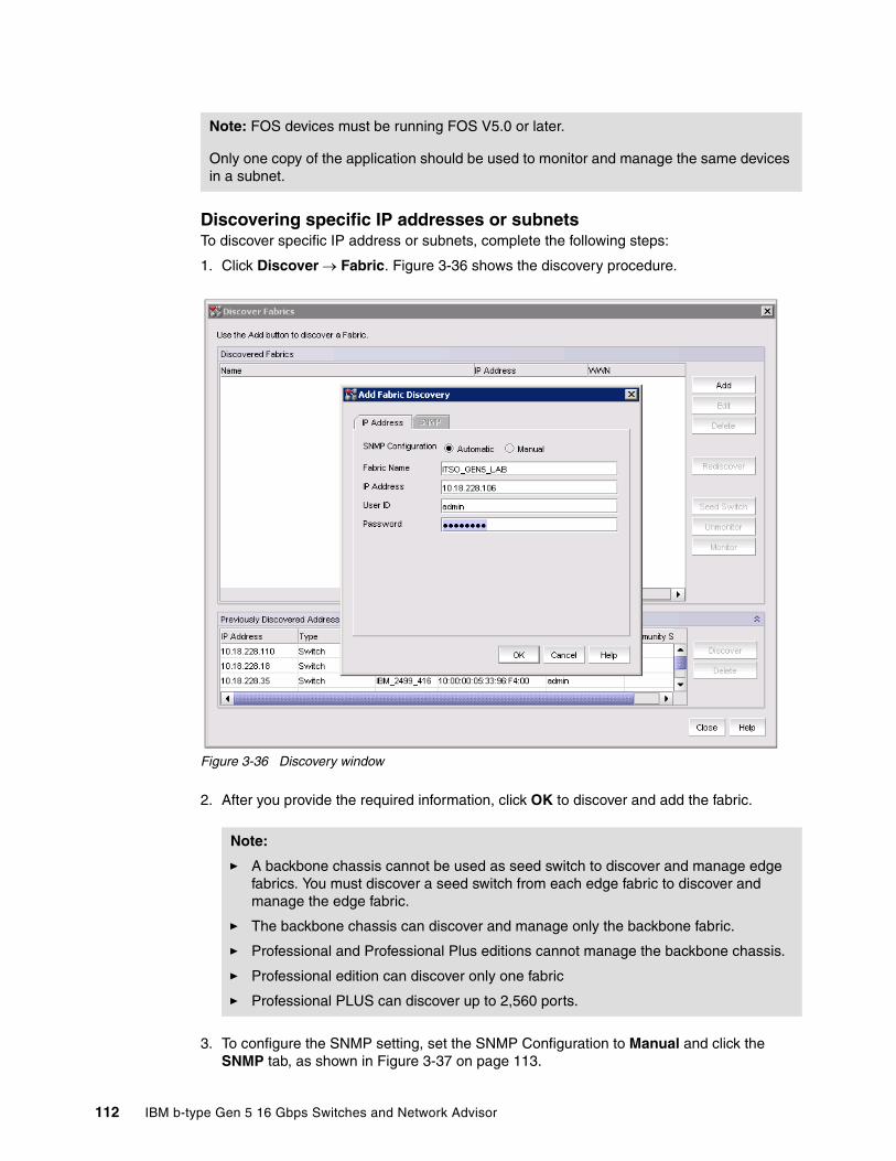
Discovering specific IP addresses or subnetsTo discover specific IP address or subnets, complete the following steps:
1. Click Discover Fabric. Figure 3-36 shows the discovery procedure.
Figure 3-36 Discovery window
2. After you provide the required information, click OK to discover and add the fabric.
3. To configure the SNMP setting, set the SNMP Configuration to Manual and click the SNMP tab, as shown in Figure 3-37 on page 113.
Note: FOS devices must be running FOS V5.0 or later.
Only one copy of the application should be used to monitor and manage the same devices in a subnet.
Note:
� A backbone chassis cannot be used as seed switch to discover and manage edge fabrics. You must discover a seed switch from each edge fabric to discover and manage the edge fabric.
� The backbone chassis can discover and manage only the backbone fabric.
� Professional and Professional Plus editions cannot manage the backbone chassis.
� Professional edition can discover only one fabric
� Professional PLUS can discover up to 2,560 ports.
112 IBM b-type Gen 5 16 Gbps Switches and Network Advisor
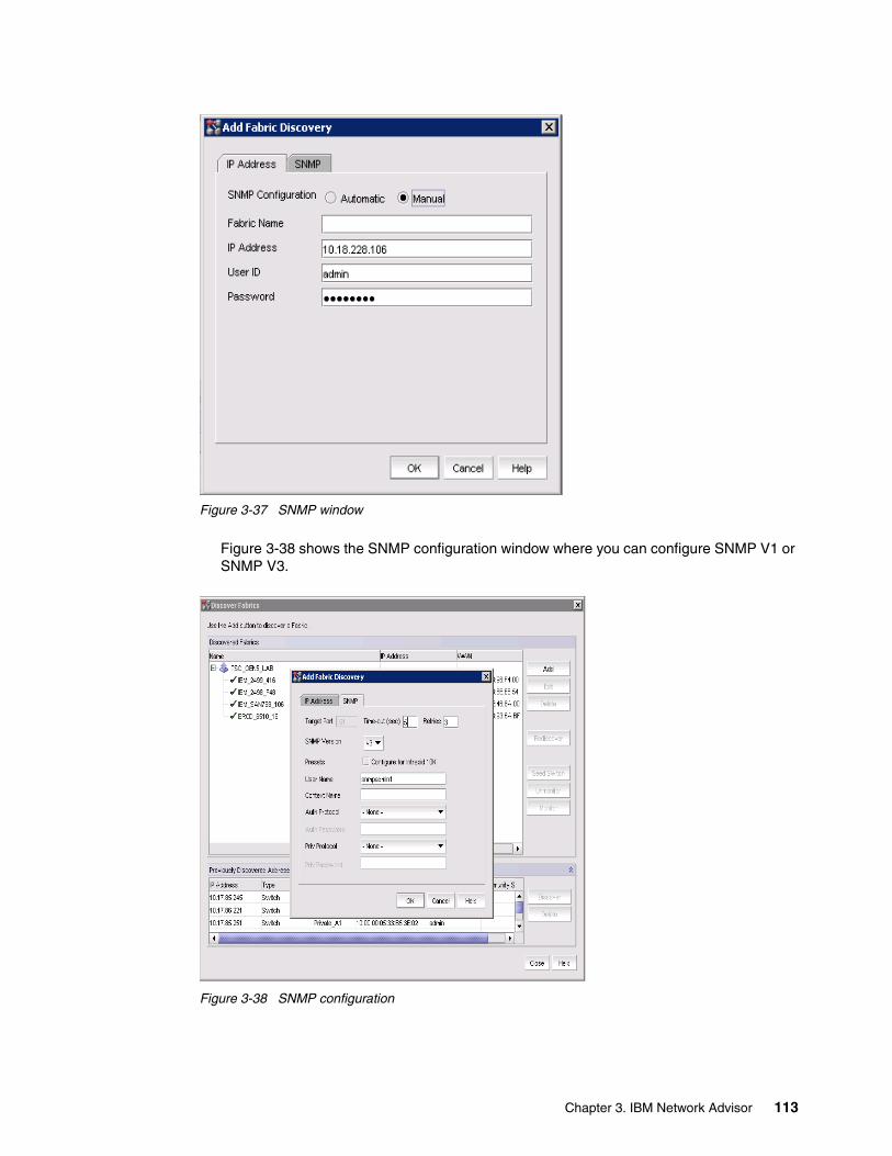
Figure 3-37 SNMP window
Figure 3-38 shows the SNMP configuration window where you can configure SNMP V1 or SNMP V3.
Figure 3-38 SNMP configuration
Chapter 3. IBM Network Advisor 113
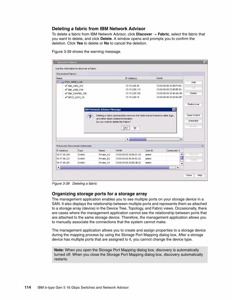
Deleting a fabric from IBM Network AdvisorTo delete a fabric from IBM Network Advisor, click Discover Fabric, select the fabric that you want to delete, and click Delete. A window opens and prompts you to confirm the deletion. Click Yes to delete or No to cancel the deletion.
Figure 3-39 shows the warning message.
Figure 3-39 Deleting a fabric
Organizing storage ports for a storage arrayThe management application enables you to see multiple ports on your storage device in a SAN. It also displays the relationship between multiple ports and represents them as attached to a storage array (device) in the Device Tree, Topology, and Fabric views. Occasionally, there are cases where the management application cannot see the relationship between ports that are attached to the same storage device. Therefore, the management application allows you to manually associate the connections that the system cannot make.
The management application allows you to create and assign properties to a storage device during the mapping process by using the Storage Port Mapping dialog box. After a storage device has multiple ports that are assigned to it, you cannot change the device type.
Note: When you open the Storage Port Mapping dialog box, discovery is automatically turned off. When you close the Storage Port Mapping dialog box, discovery automatically restarts.
114 IBM b-type Gen 5 16 Gbps Switches and Network Advisor
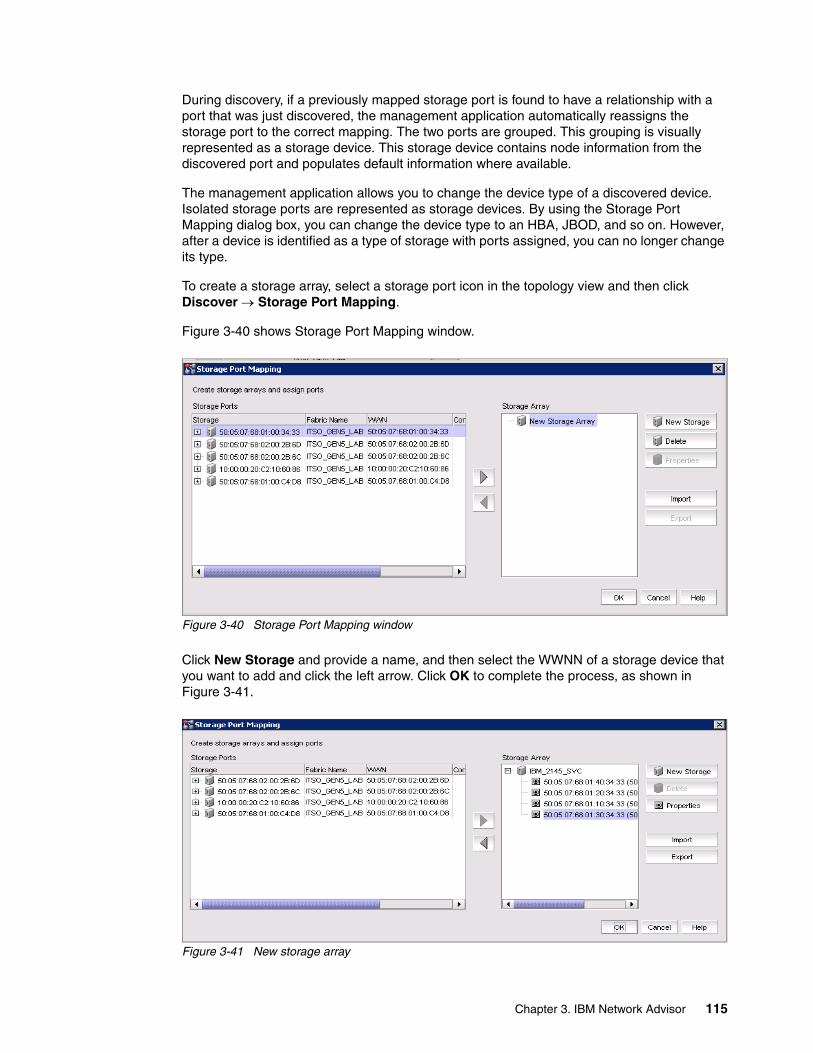
During discovery, if a previously mapped storage port is found to have a relationship with a port that was just discovered, the management application automatically reassigns the storage port to the correct mapping. The two ports are grouped. This grouping is visually represented as a storage device. This storage device contains node information from the discovered port and populates default information where available.
The management application allows you to change the device type of a discovered device. Isolated storage ports are represented as storage devices. By using the Storage Port Mapping dialog box, you can change the device type to an HBA, JBOD, and so on. However, after a device is identified as a type of storage with ports assigned, you can no longer change its type.
To create a storage array, select a storage port icon in the topology view and then click Discover Storage Port Mapping.
Figure 3-40 shows Storage Port Mapping window.
Figure 3-40 Storage Port Mapping window
Click New Storage and provide a name, and then select the WWNN of a storage device that you want to add and click the left arrow. Click OK to complete the process, as shown in Figure 3-41.
Figure 3-41 New storage array
Chapter 3. IBM Network Advisor 115

3.4 New features of IBM Network Advisor V12.0.3
The following features were introduced with IBM Network Advisor V12.0.3:
� Performance Dashboard� Frame Viewer� Port Commissioning� Bulk Port Configuration (Host Management)
3.4.1 Performance Dashboard
The Performance Dashboard provides a high-level overview of the performance of the network, which allows you to easily check the performance of devices in the network. The Performance Dashboard also provides several features to help you quickly access performance metrics and reports.
Dashboards update every 10 minutes regardless of the currently selected tab (SAN or dashboard) or the SAN size.
You can change the default size of the status widgets and performance monitors by placing the cursor on the divider until a double arrow displays. Click and drag the adjoining driver to resize the window.
Figure 3-42 shows the default Performance Dashboard. There are two ways to access it:
� Click Dashboard Performance Dashboard.� Click Monitor Performance Dashboard.
Figure 3-42 Default Performance Dashboard
116 IBM b-type Gen 5 16 Gbps Switches and Network Advisor
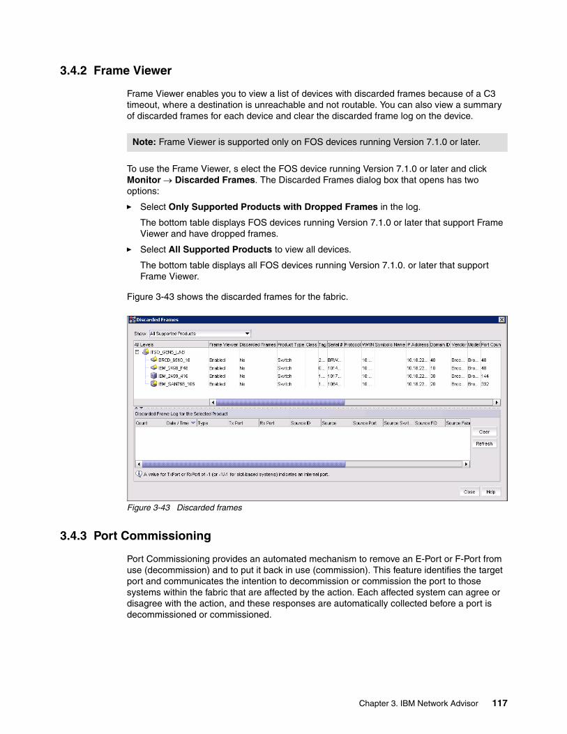
3.4.2 Frame Viewer
Frame Viewer enables you to view a list of devices with discarded frames because of a C3 timeout, where a destination is unreachable and not routable. You can also view a summary of discarded frames for each device and clear the discarded frame log on the device.
To use the Frame Viewer, s elect the FOS device running Version 7.1.0 or later and click Monitor Discarded Frames. The Discarded Frames dialog box that opens has two options:
� Select Only Supported Products with Dropped Frames in the log.
The bottom table displays FOS devices running Version 7.1.0 or later that support Frame Viewer and have dropped frames.
� Select All Supported Products to view all devices.
The bottom table displays all FOS devices running Version 7.1.0. or later that support Frame Viewer.
Figure 3-43 shows the discarded frames for the fabric.
Figure 3-43 Discarded frames
3.4.3 Port Commissioning
Port Commissioning provides an automated mechanism to remove an E-Port or F-Port from use (decommission) and to put it back in use (commission). This feature identifies the target port and communicates the intention to decommission or commission the port to those systems within the fabric that are affected by the action. Each affected system can agree or disagree with the action, and these responses are automatically collected before a port is decommissioned or commissioned.
Note: Frame Viewer is supported only on FOS devices running Version 7.1.0 or later.
Chapter 3. IBM Network Advisor 117
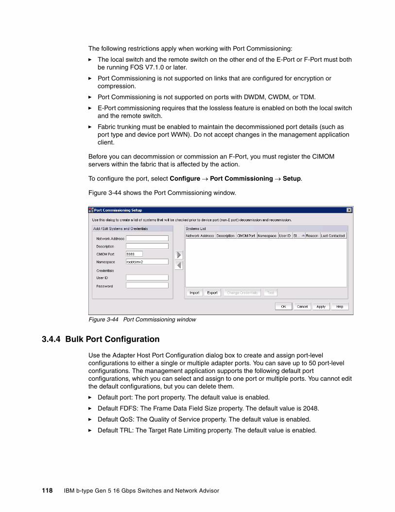
The following restrictions apply when working with Port Commissioning:
� The local switch and the remote switch on the other end of the E-Port or F-Port must both be running FOS V7.1.0 or later.
� Port Commissioning is not supported on links that are configured for encryption or compression.
� Port Commissioning is not supported on ports with DWDM, CWDM, or TDM.
� E-Port commissioning requires that the lossless feature is enabled on both the local switch and the remote switch.
� Fabric trunking must be enabled to maintain the decommissioned port details (such as port type and device port WWN). Do not accept changes in the management application client.
Before you can decommission or commission an F-Port, you must register the CIMOM servers within the fabric that is affected by the action.
To configure the port, select Configure Port Commissioning Setup.
Figure 3-44 shows the Port Commissioning window.
Figure 3-44 Port Commissioning window
3.4.4 Bulk Port Configuration
Use the Adapter Host Port Configuration dialog box to create and assign port-level configurations to either a single or multiple adapter ports. You can save up to 50 port-level configurations. The management application supports the following default port configurations, which you can select and assign to one port or multiple ports. You cannot edit the default configurations, but you can delete them.
� Default port: The port property. The default value is enabled.
� Default FDFS: The Frame Data Field Size property. The default value is 2048.
� Default QoS: The Quality of Service property. The default value is enabled.
� Default TRL: The Target Rate Limiting property. The default value is enabled.
118 IBM b-type Gen 5 16 Gbps Switches and Network Advisor

Configuring host adapter ports To create, edit, duplicate, or delete port configurations, click Configure Host Adapter ports. Make your changes.
Figure 3-45 shows the Configure Host Adapter Ports window.
Figure 3-45 Configure Host Adapter Ports window
3.5 IBM Network Advisor Dashboard
This section describes the IBM Network Advisor dashboards.
3.5.1 Dashboard overview
The dashboards (which can be found in the Dashboard tab of the Performance Dashboard window) provide a high-level overview of the network and the current state of the management devices. You can use the dashboards to easily check the status of the devices in the network. The dashboards also provide several features to help you quickly access reports, device configurations, and system logs.
The dashboards update regardless of the currently selected tab (SAN or dashboard) or the SAN size. However, data might become momentarily out of sync between the dashboards and other areas of the applications. For example, if you remove a product from the network while another user navigates from the dashboard to a more detailed view of the product, the product may not appear in the detail view.
Chapter 3. IBM Network Advisor 119

Figure 3-46 shows the dashboard.
Figure 3-46 Dashboard
Where:
1. Menu bar: Lists commands that you can perform on the dashboard. The dashboard also provides a menu to reset the dashboard back to the defaults. You can reset the dashboard back to the default settings by right-clicking and selecting Reset to Default.
2. Toolbar: Provides buttons that enable quick access to dialog boxes and functions.
3. Dashboard tab: Provides a high-level overview of the network that is managed by the management application server.
4. SAN: Displays the master log, Minimap, Connectivity map (topology), and product list.
5. Widgets: Displays the operational status, inventory status, event summary, and overall network or fabric status, and performance monitors.
6. Master log: Displays all events that have occurred on the management application.
7. Status bar: Displays the connection, port, product, fabric, special event, Call Home, and backup status, and server and user data.
3.5.2 Customizing the dashboard
From the dashboard (Dashboard or Performance Dashboard), click the customize Dashboard icon. After you click the customize Dashboard icon, a window with Status and Performance tabs opens.
6
5
4
3
2
1
7
120 IBM b-type Gen 5 16 Gbps Switches and Network Advisor
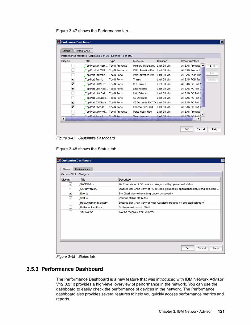
Figure 3-47 shows the Performance tab.
Figure 3-47 Customize Dashboard
Figure 3-48 shows the Status tab.
Figure 3-48 Status tab
3.5.3 Performance Dashboard
The Performance Dashboard is a new feature that was introduced with IBM Network Advisor V12.0.3. It provides a high-level overview of performance in the network. You can use the dashboard to easily check the performance of devices in the network. The Performance dashboard also provides several features to help you quickly access performance metrics and reports.
Chapter 3. IBM Network Advisor 121

The dashboards update every 10 minutes regardless of the currently selected tab (SAN or dashboard) or the SAN size. You can change the default size of the status widgets and performance monitors by placing the cursor on the divider until a double arrow displays. Click and drag the adjoining divider to resize the window. You can reset the Performance Dashboard back to the default size by right-clicking and selecting Reset to Default.
The management application provides the following pre-configured performance monitors:
� Top port C3 Discards: Table view of the C3 discards measurement (All SAN FC port collectors)
� Top port C3 discards RX TO: Table view of the C3 discards RX TO measurement (All SAN FC port collectors)
� Top port CRC errors: Table view of the CRC errors measurement (All SAN FC port collectors and All SAN TE port collectors)
� Top port Encode error out: Table view of the Encode error out measurement (All SAN FC port collectors)
� Top port errors: Table view of the error measurement (port error count collector)
� Top port link failures: Table view of the top port link failures (All SAN FC port collectors)
� Top port link resets: Table view of the top port link resets (All SAN FC port collectors)
� Top port sync losses: Table view of the top port synchronization loss (All SAN FC port collectors)
� Top port traffic: Table view of the traffic measurement (All SAN FCIP tunnel collectors, All SAN FC port collectors, port throughput collector, and All SAN TE port collectors)
� Top port utilization percentage: Table view of the port utilization percentage measurement (All SAN FCIP tunnel collectors, All SAN FC port collectors, port throughput collector, and All SAN TE port collector)
� Top product CPU utilization Table view of the CPU utilization percentage measurement (All SAN products collectors)
� Top product Memory utilization: Table view of the memory utilization percentage measurement (All SAN products collectors)
� Top product response time: Table view of the response time measurement (All SAN products collectors and System temperature collector)
� Top product response time: Table view of the response time measurement (SAN products collector)
� Top product temperature: Table view of temperature measurement (All SAN products collectors and System temperature collectors)
These pre-configured performance monitors can be turned off, hidden, and edited; however, you cannot delete the pre-configured monitors. You can also create performance monitors on the Performance Dashboard.
To start a performance dashboard, click Monitor Performance Dashboard.
User-defined performance monitorsThe Performance Dashboard makes it easy for you to customize performance monitors that are specific to your needs. You can define up to 100 performance monitors; however, you can display only up to 30 performance monitors at a time.
122 IBM b-type Gen 5 16 Gbps Switches and Network Advisor

To configure performance monitors, complete the following steps:
1. Select Monitor Performance Dashboard.
The Performance Dashboard opens in a new window
2. Click the Customize dashboard icon.
The customize Dashboard dialog box opens.
3. Click the Performance tab and click Add.
The Add Performance Dashboard monitor dialog box opens.
4. Enter a unique title for the monitor. The title can be up to 256 characters in length.
5. Select the type of monitor you are creating by clicking Monitor type Products area.
6. To add widgets to the performance monitor, click Add to navigate to the window that is shown in Figure 3-49.
Figure 3-49 Add Performance Dashboard
7. Select options from the Products or Ports, Measure, Duration, and Options panes according to your requirement. After you select your options, name the monitor and press OK.
Chapter 3. IBM Network Advisor 123

As an example, to monitor link failures on Top N-Ports for the last four hours, click Ports Top N, FC Link Failures, Duration Last 4 Hours and provide the value for N from options (in this example, N=10). After you click OK, as shown in Figure 3-50, a wizard that is called Dashboard Wizard opens.
Figure 3-50 Example for link failures
General functionsThe management application also provides the following general functions, which are applicable to all widgets and monitors:
� Performance Persistence: Any customization that you make to the Dashboard tab or Performance Dashboard tab persists in that dashboard. For example, if you customize both dashboards to display the event widget and set the range to This Hour in the dashboard tab and set it to Last 30 days in the performance dashboard, then these preferences persist when you log off and log back in again.
� Severity: Most widgets display a severity icon (the worst severity is shown) next to the widget title. The SAN status and SAN and Host inventory widgets also indicate the number of products with that severity. The event widget displays a severity icon with the highest severity event color. The status widget does not display the severity icon.
� Title bar buttons: Status widgets have the following three (left to right) title bar buttons: expand/collapse, maximize/minimize, and close. Performance monitor widgets are editable and have the following four (left to right) title bar buttons: edit, expand/collapse, maximize/minimize, and close.
� Resizing: All widgets can be resized by dragging their “grab bars”. Use the vertical grab bars between widget column to adjust the width of widgets in the adjacent column. Use the horizontal grabs to adjust the height of adjacent widget rows.
� Zoom in/Zoom out: Only widgets with a bar graph enable you to zoom in or zoom out using your mouse. To zoom in, click the upper left of the widget area on which you want to zoom in, drag the mouse to the lower right, and release the mouse button. To zoom out, click the lower right widget area on which you want to zoom out, drag the mouse to the upper left, and release the mouse button.
� Tooltips: Only widgets with pie chart or bar graph display tooltips when you pause on a section or bar.
– For the pie chart widgets, the tooltip displays the name of the category, number of items in the category, and the percentage.
124 IBM b-type Gen 5 16 Gbps Switches and Network Advisor

– For the bar graph widget, the tooltip displays the count that is represented by the selected bar.
Exporting and printing the dashboard displayYou can export or print the current dashboard display (all widgets and monitors) or a selected widget or a monitor in .png format.
� To export: Select the entire dashboard or a specific widget to export and click Export from on the toolbar.
� To print: Select the entire dashboard or a specific widget to print and click the printer icon on the toolbar.
Attaching and detaching the Dashboard tabYou can detach the Dashboard tab from the main application to display in a separate window. To detach the Dashboard tab, click Detach on the toolbar. You can move back and forth between the main application, Dashboard window, and Performance Dashboard window as needed. If you open a dialog box from any window, you must close it before you can return to the other window
Dashboard widgetsThe dashboard can be part of main application (Dashboard tab) or a separate dashboard window. The management application provides the following preconfigured status widgets:
1. Bottlenecked ports: Table view of the bottlenecked ports and the number of violations for each bottlenecked port in the SAN
2. Events: Bar chart view of events grouped by severity and range
3. Host adapter inventory: Stacked bar chart view of host adapters grouped by selected category
4. SAN Inventory: Stacked bar chart view of FC devices grouped by operational status and selected category
5. SAN Status: Pie chart view of FC devices categorized by operational status
6. Status: List view of various status attributes
7. VM Alarms: Table view of alarms received from vCenter products
3.6 Scheduling daily or weekly backups for the fabric configuration
You should back up the configuration of all fabrics in the environment daily. To schedule the daily backup of the configuration by using IBM Network Advisor, click Configure Configuration Save on Schedule.
As shown in Figure 3-51 on page 126 select the Enable Scheduled backup check box and schedule the frequency. You can choose Daily, Weekly, or Monthly, but Daily is recommended. Choose the time window to schedule the backup, and also choose the period of days you want to keep the configuration backup.
The Purge Backup can be 7 - 90 days; the default is 30 Days. You can choose all fabrics in the network by selecting the Backup all fabrics check box, or by selecting some of the switches in the network. You should collect a backup of all the fabrics in the environment.
Chapter 3. IBM Network Advisor 125
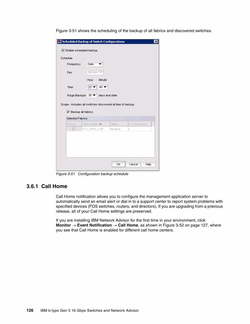
Figure 3-51 shows the scheduling of the backup of all fabrics and discovered switches.
Figure 3-51 Configuration backup schedule
3.6.1 Call Home
Call Home notification allows you to configure the management application server to automatically send an email alert or dial in to a support center to report system problems with specified devices (FOS switches, routers, and directors). If you are upgrading from a previous release, all of your Call Home settings are preserved.
If you are installing IBM Network Advisor for the first time in your environment, click Monitor Event Notification Call Home, as shown in Figure 3-52 on page 127, where you see that Call Home is enabled for different call home centers.
126 IBM b-type Gen 5 16 Gbps Switches and Network Advisor

Figure 3-52 Call Home
Clear the Enabled check boxes for the EMC, HP LAN, NetApp email, and Oracle email servers to disable or to hide them. When you clear one of these check boxes, a message is displayed: “Call Home center will be disabled. Do you want to continue?” Select Yes to continue or No to cancel.
Call Home allows you to automate tasks that occur when the Call Home event trigger is fired. When a Call Home trigger event occurs, the management application generates the following actions:
1. Sends an email alert to a specified recipient or dials in to a support center.
2. Triggers the supportsave command on the switch (if the supportsave command is enabled on the switch) before sending an alert. The supportsave location is included in the alert.
3. Adds an entry to the master log file and screen display.
4. Generates an HTML report for email-based Call Home centers.
Call Home allows you to perform the following tasks:
� Assign devices to and remove devices from the Call Home centers.
� Define filters from the list of events that are generated by FOS devices.
� Edit and remove the filters that are available in the Call Home event filters table.
� Apply filters to and remove filters from the devices individually or in groups.
� Edit individual Call Home center parameters to dial a specified phone number or email a specific recipient.
� Enable and disable individual devices from contacting the assigned Call Home centers.
Note: Call Home is supported on Windows systems for all modem and email Call Home centers and is supported on UNIX for the email Call Home centers.
Chapter 3. IBM Network Advisor 127

� Show or hide Call Home centers on the display.
� Enable or disable Call Home centers.
System requirementsCall Home requires the following hardware equipment:
� Any Windows server with an internal or external modem connection
� An analog phone line
Select Edit Centers from the Call Home window to configure the Call Home centers. After you select Edit Centers a window opens, as shown in Figure 3-53. Select Call Home Center from the drop-down list and provide the required information, such as Primary Connection, Backup Connection, and Phone Number. Click OK.
Figure 3-53 Configuring a Call Home center
128 IBM b-type Gen 5 16 Gbps Switches and Network Advisor
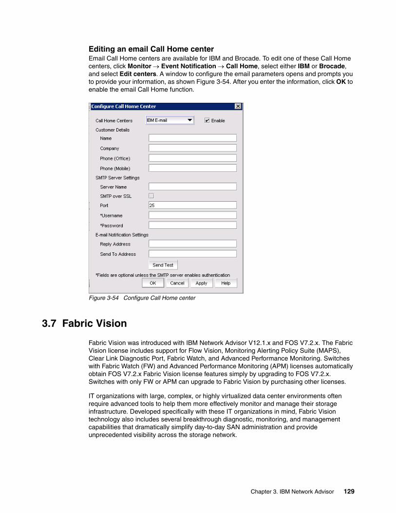
Editing an email Call Home centerEmail Call Home centers are available for IBM and Brocade. To edit one of these Call Home centers, click Monitor Event Notification Call Home, select either IBM or Brocade, and select Edit centers. A window to configure the email parameters opens and prompts you to provide your information, as shown Figure 3-54. After you enter the information, click OK to enable the email Call Home function.
Figure 3-54 Configure Call Home center
3.7 Fabric Vision
Fabric Vision was introduced with IBM Network Advisor V12.1.x and FOS V7.2.x. The Fabric Vision license includes support for Flow Vision, Monitoring Alerting Policy Suite (MAPS), Clear Link Diagnostic Port, Fabric Watch, and Advanced Performance Monitoring. Switches with Fabric Watch (FW) and Advanced Performance Monitoring (APM) licenses automatically obtain FOS V7.2.x Fabric Vision license features simply by upgrading to FOS V7.2.x. Switches with only FW or APM can upgrade to Fabric Vision by purchasing other licenses.
IT organizations with large, complex, or highly virtualized data center environments often require advanced tools to help them more effectively monitor and manage their storage infrastructure. Developed specifically with these IT organizations in mind, Fabric Vision technology also includes several breakthrough diagnostic, monitoring, and management capabilities that dramatically simplify day-to-day SAN administration and provide unprecedented visibility across the storage network.
Chapter 3. IBM Network Advisor 129

Fabric Vision is an extension of b-type Gen 5 Fibre Channel and introduces a breakthrough hardware and software solution that maximizes uptime, simplifies SAN management, and provides unprecedented visibility and insight across the storage network. Offering innovative diagnostic, monitoring, and management capabilities, Fabric Vision technology helps administrators avoid problems, maximize application performance, and reduce operational costs.
The advanced technologies and capabilities that are described in this section are available with the optional Fabric Vision technology license.
3.7.1 ClearLink Diagnostics
Brocade ClearLink Diagnostics, a patent-pending technology, uses the unique Brocade Diagnostic Port (D_Port) mode to ensure optical and signal integrity for Gen 5 Fibre Channel optics and cables, simplifying deployment and support of high performance fabrics. By pro-actively verifying the integrity of critical transceivers, organizations can quickly address any physical layer issues without the need for special optical testers.
ClearLink Diagnostics allows users to automate a battery of tests to measure and validate latency and distance across the switch links, and verify the integrity of the fiber and 16 Gbps transceivers in the fabric, either before deployment or when there are suspected physical layer issues. With ClearLink Diagnostics, only the ports that are attached to the link being tested need to go offline, leaving the rest of the ports to operate online.
In addition to switch-to-switch link validation, FOS V7.1 provides several enhancements:
� Dynamic ClearLink Diagnostics support between Gen 5 Fibre Channel switches and Brocade 1860 Fabric Adapters when running at 16 Gbps speed allows administrators to initiate tests simply by enabling them from the adapter.
� Support for Gen 5 Fibre Channel switches running in Access Gateway mode.
� Support for UltraScale chassis connectivity links on IBM SAN b-type 768B-2 and SAN 384B-2 backbones.
3.7.2 Bottleneck Detection
Bottleneck Detection identifies and alerts administrators to device or ISL congestion and abnormal levels of latency in the fabric. When it is applied to F_Ports, Bottleneck Detection can continuously monitor for medium or high levels of latency on a device port and provide notification about the nature and duration of the latency. Bottleneck Detection can also serve as a confirmation about host information when storage latencies are suspected as the cause of poor host performance. The reverse (eliminating the storage as the source of poor performance) is also true. When applied to E_Ports, Bottleneck Detection can alert administrators when it detects high levels of latency on an ISL, which is often the result of congestion or latency from elsewhere in the fabric, but also a condition that can occur as a result of device latencies from multiple flows.
Network Advisor works with Bottleneck Detection to automatically monitor and detect network congestion and latency in the fabric, providing visualization of bottlenecks in a connectivity map and product tree. Network Advisor also can show exactly which devices and hosts are impacted by a bottlenecked port.
130 IBM b-type Gen 5 16 Gbps Switches and Network Advisor

3.7.3 Flow Vision
Flow Vision enables administrators to identify, monitor, and analyze specific application and data flows to maximize performance, avoid congestion, and optimize resources.
Flow Vision includes the following features:
� Flow Monitor: Provides comprehensive visibility into flows in the fabric, including the ability to automatically learn (discover) flows and non-disruptively monitor flow performance. Users can monitor all flows from a specific host to multiple targets/LUNs or from multiple hosts to a specific target/LUN, monitor all flows across a specific ISL, or perform LUN-level monitoring of specific frame types to identify resource contention or congestion that is impacting application performance. Flow Monitor provides the following capabilities:
– Comprehensive visibility into application flows in the fabric, including the ability to learn (discover) flows automatically.
– Monitoring of application flows within a fabric at a given port.
– Statistics are associated with the specified flows to gain insights into application performance, such as transmit frame count, receive frame count, transmit throughput, receive throughput, SCSI Read frame count, SCSI Write frame count, and number of SCSI Reads and Writes per second (IOPS).
– When NPIV is used on the host, users can monitor virtual machine (VM)-to-LUN-level performance.
– Monitoring of various frame types at a switch port provides deeper insights into the storage I/O access pattern at the LUN level, reservation conflicts, and I/O errors. Examples of frame types include SCSI Read, SCSI Write, SCSI Reserve, ABTS, and BA_ACC.
– Flow Monitor is integrated with Brocade Monitoring and Alerting Policy Suite (MAPS) to enable threshold-based monitoring and alerting of flows.
Figure 3-55 shows the Flow (LUN) Level Performance monitor. It enables performance tuning and resource optimization. Earlier implementations were supported monitoring only at the storage port level.
Figure 3-55 Flow (LUN) Level Performance Monitor
Chapter 3. IBM Network Advisor 131

Figure 3-56 shows the Flow (LUN Level) frame monitoring. It acts as a built-in frame analyzer at each port, enables powerful diagnostic tests, and enables proactive monitoring and alerting. For example, you can implement Flow (LUN Level) frame monitoring to detect performance degradation in server virtualization environments by monitoring excessive SCSI reservations at a LUN level.
Figure 3-56 Flow (LUN Level) Frame Monitoring
� Flow Mirror: Can non-disruptively create copies of specific application and data flows or frame types that can be captured for deeper analysis. Flow Mirror is used for in-depth analysis of flows of interest or specific frame types, such as analysis of SCSI Reservation frames, ABTS frames, or flows going to a bottlenecked device.
Figure 3-57 shows the Ingress traffic of F-Port mirroring to the switch processor.
Figure 3-57 Mirror frames at Ingress F-Port
Figure 3-58 shows the Egress traffic of F-Port mirroring to the switch processor.
Figure 3-58 Mirror Frames at Egress F-Port
132 IBM b-type Gen 5 16 Gbps Switches and Network Advisor
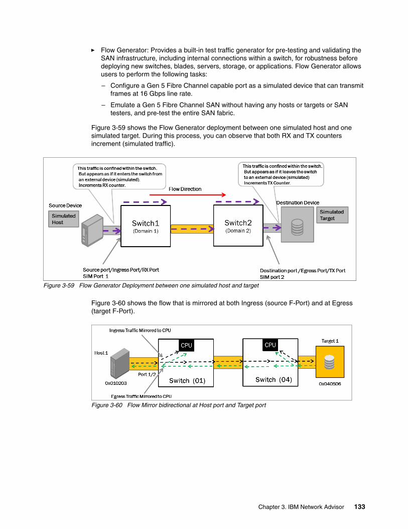
� Flow Generator: Provides a built-in test traffic generator for pre-testing and validating the SAN infrastructure, including internal connections within a switch, for robustness before deploying new switches, blades, servers, storage, or applications. Flow Generator allows users to perform the following tasks:
– Configure a Gen 5 Fibre Channel capable port as a simulated device that can transmit frames at 16 Gbps line rate.
– Emulate a Gen 5 Fibre Channel SAN without having any hosts or targets or SAN testers, and pre-test the entire SAN fabric.
Figure 3-59 shows the Flow Generator deployment between one simulated host and one simulated target. During this process, you can observe that both RX and TX counters increment (simulated traffic).
Figure 3-59 Flow Generator Deployment between one simulated host and target
Figure 3-60 shows the flow that is mirrored at both Ingress (source F-Port) and at Egress (target F-Port).
Figure 3-60 Flow Mirror bidirectional at Host port and Target port
Chapter 3. IBM Network Advisor 133

3.7.4 Monitoring Alerting Policy Suite
Monitoring Alerting Policy Suite (MAPS) provides a new and easy-to-use solution for policy-based threshold monitoring and alerting. MAPS proactively monitors the health and performance of the SAN infrastructure to ensure application uptime and availability. By using pre-built rule-/policy- based templates, MAPS simplifies threshold configuration, monitoring, and alerting. Organizations can configure the entire fabric (or multiple fabrics) at one time by using common rules and policies, or customize policies for specific ports or switch elements, all through a single window. The integrated dashboard displays an overall switch health report, along with details about out-of-policy conditions, to help administrators quickly pinpoint potential issues and easily identify trends and other behaviors occurring on a switch or fabric.
MAPS offers the following capabilities:
� Policy-based monitoring, including predefined monitoring groups and pre-validated monitoring policies that users can use. Pre-defined monitoring groups include switch ports that are attached to servers, switch ports that are attached to storage, E_Ports, short-wavelength SFPs, long-wavelength SFPs, and more. Predefined monitoring policies include aggressive, moderate, and conservative policies that are based on monitoring thresholds and actions.
� Flexibility to create custom monitoring groups, such as switch ports that are attached to high-priority applications and another group of switch ports that are attached to low-priority applications, and monitoring of each group according to its own unique rules.
� Flexible monitoring rules monitor a given counter for different threshold values and take different actions when each threshold value is crossed. For example, users can monitor a CRC error counter at a switch port and generate a RASlog when the error rate reaches two per minute, send an email notification when the error rate is at five per minute, and fence a port when the error rate exceeds ten per minute.
� Ability to monitor both sudden failures and gradually deteriorating conditions in the switch. For example, MAPS can detect and alert users if a CRC error counter suddenly increases to five per minute, or gradually increases to five per day.
� Support for multiple monitoring categories, enabling monitoring of the overall switch status, switch ports, SFPs, port blades, core blades, switch power supplies, fans, temperature sensors, security policy violations, fabric reconfigurations, processor and memory utilization, traffic performance, FCIP circuit health, and more.
� Support for multiple alerting mechanisms (RAS logs, SNMP traps, and email notifications) and actions such as port fencing when errors exceed the specified threshold.
The CLI dashboard offers the following capabilities:
� A dashboard of health and error statistics to provide at-a-glance views of switch status and various conditions that are contributing to the switch status, enabling users to get instant visibility into any hot spots at a switch level and take corrective actions.
� Overall status of the switch health and the status of each monitoring category, including any out-of-range conditions and the rules that were triggered.
� Historical information about the switch status for up to the last seven days. The CLI dashboard automatically provides raw counter information for a various error counters.
Bottleneck detection integration with MAPS dashboard: Bottleneck detection information is integrated with the MAPS dashboard, showing bottleneck events that are detected by the Bottleneck Monitor and transient bottlenecks that are not detected by the Bottleneck Monitor. This enables users to get at an instant view of the bottlenecked ports in the switch, and enables rapid problem resolution.
134 IBM b-type Gen 5 16 Gbps Switches and Network Advisor

Proactive flow monitoring using MAPS: MAPS can monitor flows that are established within Flow Vision and generate alerts that are based on user-defined rules, enabling users to monitor and be alerted when established thresholds are exceeded.
Automated migration of Fabric Watch configurations to MAPS: Organizations currently using Fabric Watch can automatically import existing thresholds into a MAPS policy, enabling seamless migration from Fabric Watch to MAPS to access the new MAPS capabilities and usability enhancements.
3.7.5 Simplified management and reporting
Fabric Vision technology is tightly integrated with IBM Network Advisor, providing customizable health and performance dashboard views to pinpoint problems faster, simplify SAN configuration and management, and reduce operational costs. Through Brocade Network Advisor, administrators can perform the following tasks:
� Quickly and easily configure and monitor data center fabrics based on MAPS groups and policies.
� Identify, monitor, and analyze data and application flows to maximize performance.
� Reduce the time that is spent on repetitive tasks by deploying MAPS policies and rules across the fabric, or multiple fabrics, from a single window.
� Run diagnostic tests on optics and cables to quickly identify and isolate potential fabric issues.
� Automatically monitor and detect network congestion in the fabric, and identify which devices or hosts are impacted by a bottlenecked port.
To support performance analysis and capacity planning activities, administrators can use the real-time and historical end-to-end performance data that is collected through IBM Network Advisor. They can quickly identify the most demanding traffic flows in the fabric, get a current snapshot of Top Talkers, or trend Top Talkers over time. Administrators can view end-to-end performance and Top Talker information directly in IBM Network Advisor or export it to other applications for reporting, such as Microsoft Excel and Crystal Reports.
3.7.6 Investment protection
Organizations that have both Advanced Performance Monitoring and Fabric Watch installed automatically receive Fabric Vision technology capabilities with FOS V7.2.0 or higher without having the Fabric Vision technology license installed. Organizations that have either Fabric Watch or Advanced Performance Monitoring installed (but not both) and want Fabric Vision technology capabilities, including MAPS and Flow Vision, can upgrade to Fabric Vision technology by purchasing and installing the other license.
3.8 Using MAPS with IBM Network Advisor
Before you can use IBM Network Advisor to manage your environment, your environment must be discovered. For more information about discovering and adding fabrics to IBM Network Advisor. After you add the devices, click Monitor Fabric Vision Maps Enable.
Chapter 3. IBM Network Advisor 135

As shown in Figure 3-61 select the switches and click the right arrow to move the switches. After you move the switches, click OK to enable MAPS on the switches.
Figure 3-61 Enable MAPS window
IBM Network Advisor can enable MAPS on multiple chassis at once. You do not need to manually convert the Fabric Watch policies either. After you click OK, a window opens and displays the following
“MAPS will be enabled on the selected chassis. This operation cannot be reversed. Do you want to continue?”.
Select Yes to continue. After you complete the operation, as shown in Figure 3-62, you can observe the messages about the conversion of Fabric Watch thresholds to MAPS.
Figure 3-62 Conversion messages
3.8.1 Configuring MAPS by using IBM Network Advisor
As described in 3.8, “Using MAPS with IBM Network Advisor” on page 135, after you enable MAPS in the navigation tree at the top of the window, click Monitor Fabric Vision MAPS Configure.
136 IBM b-type Gen 5 16 Gbps Switches and Network Advisor
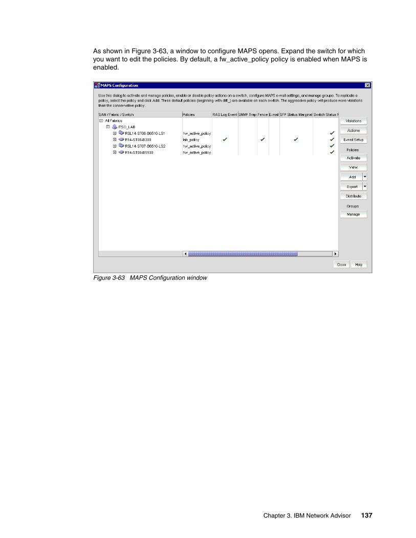
As shown in Figure 3-63, a window to configure MAPS opens. Expand the switch for which you want to edit the policies. By default, a fw_active_policy policy is enabled when MAPS is enabled.
Figure 3-63 MAPS Configuration window
Chapter 3. IBM Network Advisor 137
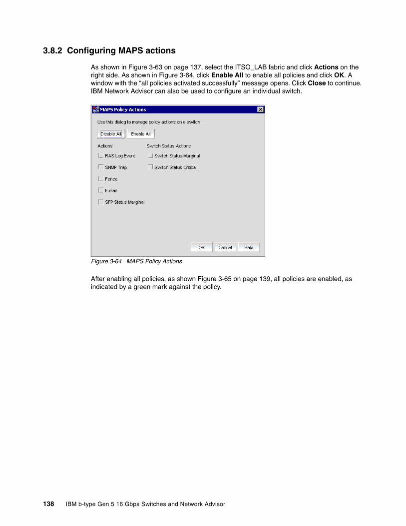
3.8.2 Configuring MAPS actions
As shown in Figure 3-63 on page 137, select the ITSO_LAB fabric and click Actions on the right side. As shown in Figure 3-64, click Enable All to enable all policies and click OK. A window with the “all policies activated successfully” message opens. Click Close to continue. IBM Network Advisor can also be used to configure an individual switch.
Figure 3-64 MAPS Policy Actions
After enabling all policies, as shown Figure 3-65 on page 139, all policies are enabled, as indicated by a green mark against the policy.
138 IBM b-type Gen 5 16 Gbps Switches and Network Advisor

Figure 3-65 MAPS configuration with all policies enabled
3.8.3 Creating policies and rules
IBM Network Advisor does not support managing policies on a fabric-wide basis. Instead, policies and rules are created on an individual switch, and they can be distributed to the rest of the switches in the fabric.
Chapter 3. IBM Network Advisor 139
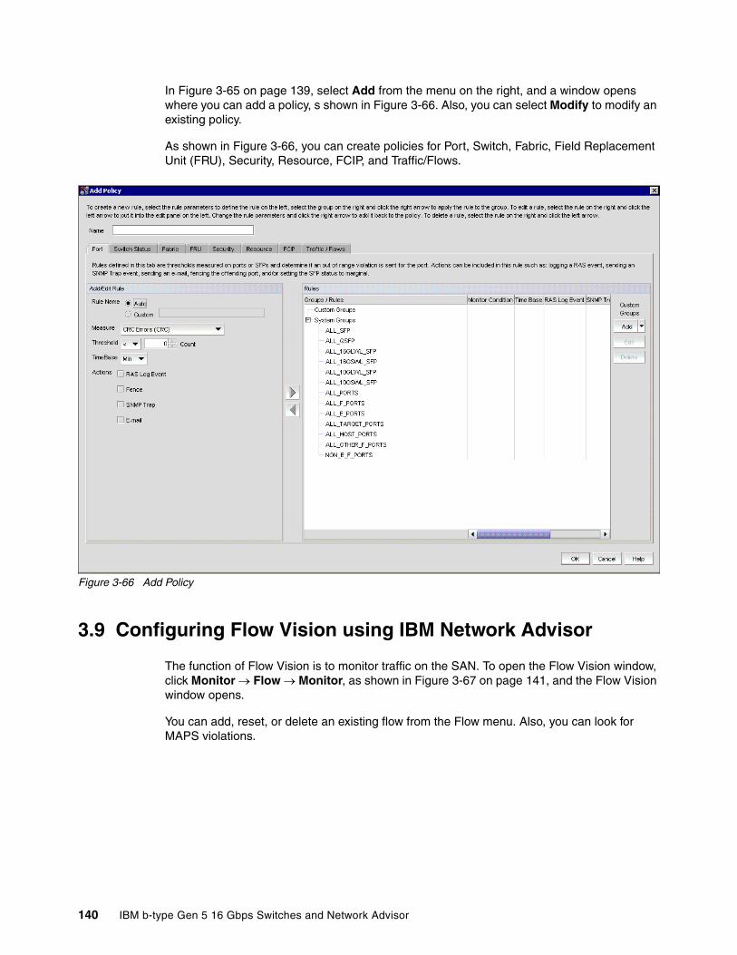
In Figure 3-65 on page 139, select Add from the menu on the right, and a window opens where you can add a policy, s shown in Figure 3-66. Also, you can select Modify to modify an existing policy.
As shown in Figure 3-66, you can create policies for Port, Switch, Fabric, Field Replacement Unit (FRU), Security, Resource, FCIP, and Traffic/Flows.
Figure 3-66 Add Policy
3.9 Configuring Flow Vision using IBM Network Advisor
The function of Flow Vision is to monitor traffic on the SAN. To open the Flow Vision window, click Monitor Flow Monitor, as shown in Figure 3-67 on page 141, and the Flow Vision window opens.
You can add, reset, or delete an existing flow from the Flow menu. Also, you can look for MAPS violations.
140 IBM b-type Gen 5 16 Gbps Switches and Network Advisor
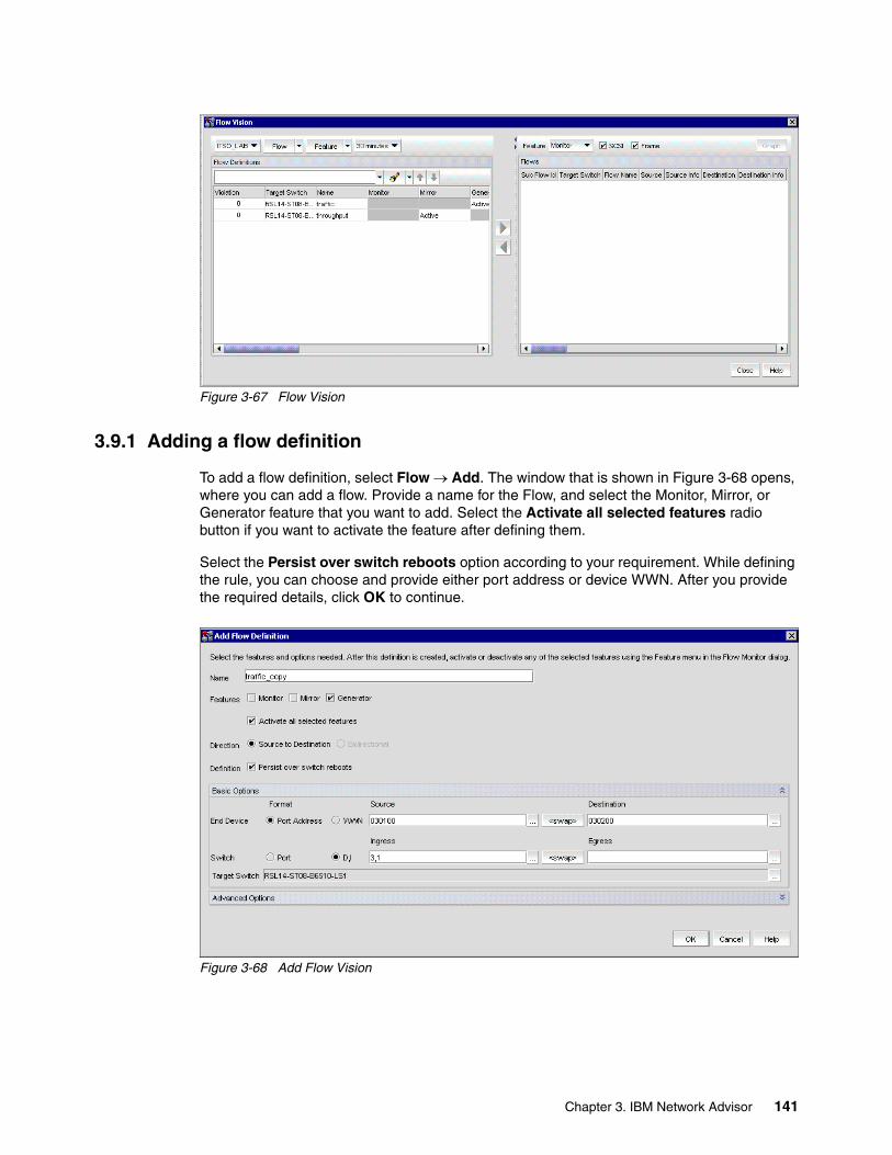
Figure 3-67 Flow Vision
3.9.1 Adding a flow definition
To add a flow definition, select Flow Add. The window that is shown in Figure 3-68 opens, where you can add a flow. Provide a name for the Flow, and select the Monitor, Mirror, or Generator feature that you want to add. Select the Activate all selected features radio button if you want to activate the feature after defining them.
Select the Persist over switch reboots option according to your requirement. While defining the rule, you can choose and provide either port address or device WWN. After you provide the required details, click OK to continue.
Figure 3-68 Add Flow Vision
Chapter 3. IBM Network Advisor 141

After you define the policy, as shown in Figure 3-69, select the policy and click the right arrow to set the monitor. Select SCSI and Frame to monitor if you want to do so. Also, you can generate a graph by clicking Graph.
Figure 3-69 Flow Vision definition
142 IBM b-type Gen 5 16 Gbps Switches and Network Advisor
Chapter 4. Initial switch setup and configuration
This chapter describes the initial setup and configuration of the IBM b-type switches and directors.
4
© Copyright IBM Corp. 2014. All rights reserved. 143

4.1 Initial setup
Before you configure any IBM System Storage SAN switch, it must be physically assembled, racked, and connected to the appropriate electrical outlet and network. The hardware requirements and specifications can be found in the specific b-type hardware installation guide that comes with the product.
After the SAN switch is physically installed and powered on, some initial configuration parameters must be set. All of the b-type switches require the same initial setup. The fundamental steps have not changed from the earlier switch models.
4.1.1 Configuring the IBM System Storage fabric backbone
The IBM System Storage fabric backbone must be configured before it is connected to the fabric, and all of the configuration commands must be entered through the active CP blade. The IBM System Networking SAN768B-2 configuration includes the following settings:
� IP address� Switch name� Chassis name� Domain ID� PID mode
Establishing a serial connection to the SAN768B-2To establish a serial connection to the console port on a SAN768B-2, complete the following steps:
1. Verify that the SAN768B-2 is powered on and that the power-on self test (POST) is complete by verifying that all power LED indicators on the port, control processor, and core switch blades display a steady green light.
2. Remove the shipping cap from the CONSOLE port on the active CP. Use the serial cable that is provided with the SAN768B-2 to connect the CONSOLE port on the active CP to a computer workstation. The active CP blade is indicated by an illuminated (blue) LED.
3. Access the SAN768B-2 by using a terminal emulator application (such as HyperTerminal in a Windows environment or tip in a UNIX environment).
4. Disable any serial communication programs running on the workstation (such as synchronization programs).
5. Open a terminal emulator application (such as HyperTerminal on a PC, or term, tip, or kermit in a UNIX environment), and configure the application as follows:
– In a Windows environment, set the values that are shown in Table 4-1.
Table 4-1 Serial connections configuration settings
Parameter Value
Bits per second 9600
Data bits 8
Parity None
Stop bits 1
Flow control None
144 IBM b-type Gen 5 16 Gbps Switches and Network Advisor

– In a UNIX environment, enter the following string at the prompt:
tip /dev/ttyb -9600
If ttyb is already in use, use ttya instead and enter the following string at the prompt:
tip /dev/ttya -9600
When the terminal emulator application stops reporting information, press Enter. You receive the following login prompt:
CP0 Console Login:
6. Log in to the SAN768B-2 as admin. The default password is password. At the initial login, which is shown below, you are prompted to enter a new admin user and user passwords (changing the password is optional, but recommended).
Fabric OS (swDir)swDir login: adminPassword:Change your passwords now.Use Control-C to exit or press 'Enter' key to proceed.swDir:admin>
Configuring IP addressesThe SAN768B-2 requires three IP addresses, which are configured by running the ipAddrSet command. IP addresses are required for both CP blades (CP0 and CP1) and for the chassis management IP (shown as SWITCH under the ipAddrShow command) in the SAN768B-2.
After you are logged in to the active CP using the Serial cable (as described in “Establishing a serial connection to the SAN768B-2” on page 144), complete the following steps:
1. Set up the Chassis IP address by running the following command:
swDir:admin> ipAddrSet -chassis
Enter the information at the prompts. Specify the -chassis IP address.
2. Set up the CP0 IP address by running the ipaddrset -cp 0 command:
swDir:admin> ipAddrSet -cp 0
Enter the information at the prompts.
3. Set up the CP1 IP address by running the ipaddrset -cp 1 command:
swDir:admin> ipAddrSet -cp 1
Enter the information at the prompts.
Note: Passwords can be 8 - 40 characters. They must begin with an alphabetic character. They can include numeric characters, the dot (.), and the underscore (_) only. Passwords are case-sensitive, and they are not displayed when you enter them on the command line.
For more information about passwords, see the Brocade Fabric OS Administrator’s Guide, found at http://my.brocade.com.
Note: Here are the default IP addresses and host names for the SAN768B-2:
� 10.77.77.75 / CP0 (the CP blade in slot 6 at the time of configuration)� 10.77.77.74 / CP1 (the CP blade in slot 7 at the time of configuration)
Chapter 4. Initial switch setup and configuration 145

Here is an example IP configuration:
swDir:admin> ipaddrset -chassisEthernet IP address [0.0.0.0]: 123.123.123.120Ethernet Subnetmask [0.0.0.0]: 123.123.123.123Fibre Channel IP address [0.0.0.0]:Fibre Channel Subnetmask [0.0.0.0]:Issuing gratuitous ARP...Done.Committing configuration...Done.
swDir:admin> ipaddrset -cp 0Host Name [cp0]:Ethernet IP address [10.77.77.75]: 123.123.123.121Ethernet Subnetmask [0.0.0.0]: 123.123.123.123Gateway IP address [0.0.0.0]: 123.123.123.124IP address is being changed...Done.Committing configuration...Done.
swDir:admin> ipaddrset -cp 1Host Name [cp1]:Ethernet IP address [10.77.77.74]: 123.123.123.122Ethernet Subnetmask [0.0.0.0]: 123.123.123.123Gateway IP address [0.0.0.0]: 123.123.123.124IP address of remote CP is being changed...Done.Committing configuration...Done.
After you use a serial connection to configure the IP addresses for the SAN768B-2, you can connect the active CP blade to the local area network (LAN) and complete the configuration using either a serial session, Telnet, SSH, or a management application such as Web Tools or IBM Network Advisor.
Customizing a switch nameThe switch name of the SAN768B-2 can be up to 30 characters when you use Fabric OS (FOS) V6.3.0 or later; it can include letters, numbers, hyphens, and underscore characters, and must begin with a letter.
Enter switchName followed by the new name in double quotation marks:
swDir:admin> switchName "ItsoSANswitch1"Committing configuration...Done.ItsoSANswitch1:admin>
Customizing a chassis nameThe chassis name of the SAN768B-2 can be up to 15 characters. It can include letters, numbers, hyphens, and underscore characters and must begin with a letter.
To customize a chassis name, complete the following steps:
1. Enter chassisName followed by the new name in double quotation marks:
ItsoSANswitch1:admin> chassisname "SAN768B-2_chassis"Committing configuration...Done.
Note: The addresses 10.0.0.0 - 10.0.0.255 are reserved and used internally by the SAN768B-2. External IPs must not use these addresses.
146 IBM b-type Gen 5 16 Gbps Switches and Network Advisor

2. Enter chassisName by itself to show the name:
ItsoSANswitch1:admin> chassisnameSAN768B-2_chassis
Setting the domain IDEach switch in the fabric must have a unique domain ID. The domain ID can be manually set by the configure command or can be automatically set. The default domain ID for the SAN768B-2 is 1. Run the fabricShow command to view the assigned domain IDs.
To set the domain ID, run the following steps:
1. Enter switchDisable to disable the SAN switch:
ItsoSANswitch1:admin> switchDisable
2. Enter configure:
ItsoSANswitch1:admin> configure
3. Enter y at the Fabric parameters prompt:
Fabric parameters (yes, y, no, n): [no] y
4. Enter a unique domain ID:
Domain: (1.239) [1] 2
5. Complete the remaining prompts or press Ctrl+D to accept the settings and exit.
6. Enter switchEnable to reenable the switch:
ItsoSANswitch1:admin> switchEnable
Verifying the PID modeBefore you connect the SAN768B-2 to the fabric, verify that the port identifier (PID) mode on the switch matches the other switches in the fabric. This setting must be identical for all switches in the fabric and is set by running configure.
4.1.2 IBM System Storage b-type switch initial configuration
The following configuration instructions are valid for the Gen 5 b-type switches:
� IBM System Networking SAN24B-5 (2498-F24, 2498-X24, and 2498-24G)
� IBM System Networking SAN48B-5 (2498-F48)
� IBM System Networking SAN96B-5 (2498-F96 / 2498-N96)
After you have set up the SAN switch in a rack and powered on the switch, it is time to apply the basic configuration. You can use the EZSwitchSetup (described in 4.1.3, “EZSwitchSetup initial configuration” on page 152) to complete the basic configuration. If you do not want to use EZSwitchSetup, continue with the instructions in this section.
The SAN switch boot process requires several minutes to boot and complete the POST. After the POST is complete, verify that the power and status LEDs on the SAN switches (port side) are green.
Chapter 4. Initial switch setup and configuration 147
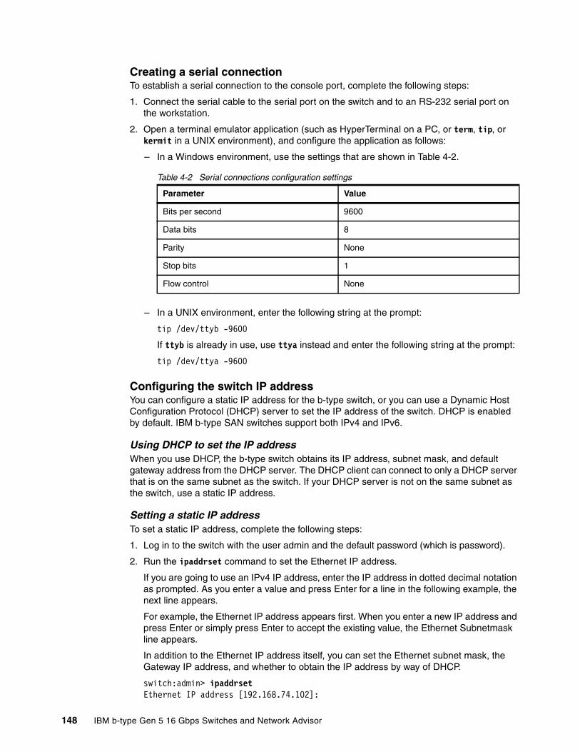
Creating a serial connectionTo establish a serial connection to the console port, complete the following steps:
1. Connect the serial cable to the serial port on the switch and to an RS-232 serial port on the workstation.
2. Open a terminal emulator application (such as HyperTerminal on a PC, or term, tip, or kermit in a UNIX environment), and configure the application as follows:
– In a Windows environment, use the settings that are shown in Table 4-2.
Table 4-2 Serial connections configuration settings
– In a UNIX environment, enter the following string at the prompt:
tip /dev/ttyb -9600
If ttyb is already in use, use ttya instead and enter the following string at the prompt:
tip /dev/ttya -9600
Configuring the switch IP addressYou can configure a static IP address for the b-type switch, or you can use a Dynamic Host Configuration Protocol (DHCP) server to set the IP address of the switch. DHCP is enabled by default. IBM b-type SAN switches support both IPv4 and IPv6.
Using DHCP to set the IP addressWhen you use DHCP, the b-type switch obtains its IP address, subnet mask, and default gateway address from the DHCP server. The DHCP client can connect to only a DHCP server that is on the same subnet as the switch. If your DHCP server is not on the same subnet as the switch, use a static IP address.
Setting a static IP addressTo set a static IP address, complete the following steps:
1. Log in to the switch with the user admin and the default password (which is password).
2. Run the ipaddrset command to set the Ethernet IP address.
If you are going to use an IPv4 IP address, enter the IP address in dotted decimal notation as prompted. As you enter a value and press Enter for a line in the following example, the next line appears.
For example, the Ethernet IP address appears first. When you enter a new IP address and press Enter or simply press Enter to accept the existing value, the Ethernet Subnetmask line appears.
In addition to the Ethernet IP address itself, you can set the Ethernet subnet mask, the Gateway IP address, and whether to obtain the IP address by way of DHCP.
switch:admin> ipaddrsetEthernet IP address [192.168.74.102]:
Parameter Value
Bits per second 9600
Data bits 8
Parity None
Stop bits 1
Flow control None
148 IBM b-type Gen 5 16 Gbps Switches and Network Advisor

Ethernet Subnetmask [255.255.255.0]:Gateway IP address [192.168.74.1]:DHCP [Off]: off
If you are going to use an IPv6 address, enter the network information in semicolon-separated notation as a stand-alone command:
switch:admin> ipaddrset -ipv6 --add 1080::8:800:200C:417A/64IP address is being changed...Done.
Date and time settingsThe b-type switches maintain the current date and time inside a battery-backed real-time clock (RTC) circuit. Date and time are used for timestamping log events. The switch’s operation does not depend on the date and time; a b-type SAN switch with an incorrect date and time value still functions correctly. However, because the date and time are used for logging, error detection, and troubleshooting, you should set the date and time correctly.
Time zonesYou can set the time zone for the switch by name. You can select continent, country, or time zone region names.
If the time zone is not set with the named options, the switch retains the offset time zone settings. This is a number of hours that are offset from Greenwich Mean Time (GMT). If you have set the time zone with a name, you can revert to the offset format if you choose.
You can set the time zone for a switch by running tsTimeZone. The tsTimeZone command allows you to perform the following tasks:
� Display all of the time zones that are supported in the firmware.
� Set the time zone based on a country and city combination or based on a time zone ID, such as PST.
For more information about the tsTimeZone command, see the Fabric OS Command Reference, found at http://my.brocade.com.
The time zone setting has the following characteristics:
� You can view the time zone settings. However, only those users with administrative permissions can set the time zones.
� The tsTimeZone command automatically adjusts for daylight saving time.
� Changing the time zone on a switch updates the local time zone setup and is reflected in local time calculations.
� By default, all switches are in the GMT time zone (0,0). If all switches in a fabric are in one time zone, it is possible for you to keep the time zone setup at the default setting.
� System services that have started reflect the time zone changes only after the next reboot.
� Time zone settings persist across failover for high availability.
Local time synchronizationYou can synchronize the local time of the principal or primary fabric configuration server (FCS) switch to a maximum of eight external Network Time Protocol (NTP) servers. To keep the time in your SAN current, keep the time of the principal or primary FCS switch synchronized with at least one external NTP server. The other switches in the fabric automatically take their time from the principal or primary FCS switch.
Chapter 4. Initial switch setup and configuration 149

All switches in the fabric maintain the current clock server IP address in non-volatile memory. By default, this value is LOCL, which is the local clock server of the Principal (when FCS is not enabled) or primary (when FCS is enabled) switch. Changes to the clock server value on the principal or primary switch are propagated to all switches in the fabric.
When a new switch enters the fabric, the time server daemon of the principal or primary switch sends out the addresses of all existing clock servers and the time to the new switch. If a switch with FOS V5.3.0 or later enters the fabric, it can store the list of all the clock server addresses; switches running FOS versions earlier than Version 5.3.0 ignore the new list parameter in the payload and updates only the active server address.
If the active NTP server configured is IPv6, then distributing the IP address in the fabric is not possible to switches with versions earlier than FOS V5.3.0 because IPv6 is supported only for FOS V5.3.0 and later. The default value LOCL is distributed to switches earlier than FOS V5.3.0.
The tsClockServer command accepts multiple server addresses in IPv4, IPv6, or DNS name formats. When multiple NTP server addresses are passed, tsClockServer sets the first obtainable address as the active NTP server. The rest is stored as backup servers that can take over if the active NTP server fails. The principal or primary switch synchronizes its time with the NTP server every 64 seconds.
Setting the dateTo set the date, complete the following steps:
1. Log in to the switch with the admin user and the default password (which is password).
2. Enter the date command with the following syntax:
date "mmddHHMMyy"
The values are:
– mm is the month. Valid values are 01 - 12.
– dd is the date. Valid values are 01 - 31.
– HH is the hour. Valid values are 00 - 23.
– MM is minutes. Valid values are 00 - 59.
– yy is the year. Valid values are 00 - 99 (values greater than 69 are interpreted as 1970 through 1999, and values less than 70 are interpreted as 2000 through 2069).
Here is some example output of the command:
switch:admin> dateFri Sep 28 17:01:48 UTC 2007switch:admin> date "0913123013"Fri Sep 13 12:30:00 UTC 2013switch:admin>
Setting time zonesYou must perform the procedure on all switches for which the time zone must be set. However, you need to set only the time zone once on each switch because the value is written to nonvolatile memory.
Use one of the two following procedures to set the time zone. The first procedure requires you to select the actual time zone and the second requires you to select the country location of the switch.
150 IBM b-type Gen 5 16 Gbps Switches and Network Advisor

� The following procedure describes how to set the current time zone to Central Standard time by using timezonename mode.
Use timezonename to set the time zone by time zone ID, such as PST or Country/City.
The following example shows how to change the time zone to US/Central. The tsTimeZone command by itself display the current time zone.
switch:admin> tstimezoneTime Zone: US/Pacificswitch:admin> tstimezone US/Centralswitch:admin> tstimezoneTime Zone: US/Central
� The following procedure describes how to set the current time zone to Pacific Standard Time using interactive mode:
a. Enter the tsTimeZone command as follows:
switch:admin> tstimezone --interactive
b. You are prompted to select a general location from a list.
Identify a location so that time zone rules can be set correctly.
c. Enter the appropriate number from the list that appears or press Ctrl-D to quit.
d. At the prompt, select a country location from the list.
e. At the prompt, enter the appropriate number from the list to specify the time zone region or press Ctrl-D to quit.
Synchronizing local time using NTPTo synchronize the local time using NTP, complete the following steps:
1. Log in to the switch using the default password (which is password).
2. Enter the tsClockServer command:
switch:admin> tsclockserver "<ntp1;ntp2>"
In the syntax, ntp1 is the IP address or DNS name of the first NTP server, which the switch must be able to access. The value ntp2 is the name of the second NTP server and is optional. The entire operand “<ntp1;ntp2>” is optional; by default, this value is LOCL, which uses the local clock of the principal or primary switch as the clock server.
switch:admin> tsclockserverLOCLswitch:admin> tsclockserver "132.163.135.131"switch:admin> tsclockserver132.163.135.131switch:admin>
The following example shows how to set up more than one NTP server using a DNS name:
switch:admin> tsclockserver "10.32.170.1;10.32.170.2;ntp.localdomain.net"Updating Clock Server configuration...done.Updated with the NTP servers
Note: Changes to the clock server value on the principal or primary FCS switch are propagated to all switches in the fabric.
Chapter 4. Initial switch setup and configuration 151
4.1.3 EZSwitchSetup initial configuration
EZSwitchSetup is an easy-to-use graphical user interface application for setting up and managing your switch. It has the following components:
� EZSwitchSetup wizard (on the installation CD)
� EZSwitchSetup switch configuration wizard
� EZSwitchSetup Switch Manager
The following section covers only the EZSwitchSetup Switch Configuration wizard. All instructions are based on Version 7.2.0 of EZSwitchSetup.
Before you begin, confirm that your switch model is compatible with the EZSwitchSetup version. Version 7.2.0 is compatible with the following Gen 4 and Gen 5 switch models:
� SAN24B-5� SAN48B-5� SAN96B-5� SAN24B-4� SAN40B-4� SAN80B-4
For full compatibility, see the EZSwitchSetp Administrator’s Guide, found at http://my.brocade.com.
Before you begin, you must obtain an IP address, subnet mask, and default gateway address for the switch. Then, complete the following steps:
1. Install the EZSwitchSetup wizard, which is on the EZSwitchSetup installation CD. Insert the EZSwitchSetup CD into the CD-ROM drive of your setup computer.
– On Windows: The installer automatically starts in about a minute.
– On Linux: Navigate to the following path on the CD-ROM:
CDROM_Path/CDROM_Installers/Linux/Disk1/InstData/VM/install.bin
2. Install EZSwitchSetup by following the directions that display. The installation takes a few minutes after you click OK.
152 IBM b-type Gen 5 16 Gbps Switches and Network Advisor

3. Click Done on the last window (see Figure 4-1) to exit the installer.
Figure 4-1 EZswitchSetup installation summary
Starting the EZSwitchSetup wizardTo start the EZSwitchSertup wizard, complete one of the following actions:
� On Windows: EZSwitchSetup starts automatically after it is installed. If it does not, then click Start Programs EZSwitchSetup EZSwitchSetup.
� On Linux: EZSwitchSetup does not start automatically, so you must start it manually by navigating to the following parth on the CD-ROM:
CDROM_Path/CDROM_Installers/Linux/Disk1/InstData/VM/install.bin
Note: The Linux installation requires root access.
Chapter 4. Initial switch setup and configuration 153

Figure 4-2 shows the Introduction window.
Figure 4-2 EZSwitchSetup Introduction window
Connecting cablesTo connect the switch cables, complete the following steps:
1. Choose the method to connect to your LAN.
You can use a serial connection or an Ethernet connection to your LAN to set the IP address for the switch. The Ethernet connection is more convenient and preferred. Use the serial connection if it is not possible or not convenient to connect the host on the same subnet as the switch.
2. Click Next.
154 IBM b-type Gen 5 16 Gbps Switches and Network Advisor

Figure 4-3 shows the Connect Cables window (Ethernet version, without serial cable)
Figure 4-3 Connect Cables window
3. Connect the power cord to the switch and plug it in to a power source. The switch power and status LEDs display amber and then change to green, which usually takes from one to three minutes.
4. Connect an Ethernet cable from the switch to the LAN you want to use for your management connection through an Ethernet hub or switch. If you chose to use your Ethernet connection for setup in step 1 on page 154, this is the connection that you use. If you chose the serial cable connection in step 1 on page 154, you should still connect the Ethernet cable so the Ethernet connection is available when you start the EZSwitchSetup Switch Manager.
5. If you are using a serial connection for setup, connect your setup computer to the serial port on the switch by using the serial cable that shipped with the switch. If you cannot find the serial cable that came with the switch, you must find one that has the appropriate connectors. Do not use a null-modem cable. Here are the serial connection settings:
– Bits per second: 9600– Tidbits: 8– Parity: None– Stop bits: 1– Flow control: None
6. Click Next.
Chapter 4. Initial switch setup and configuration 155
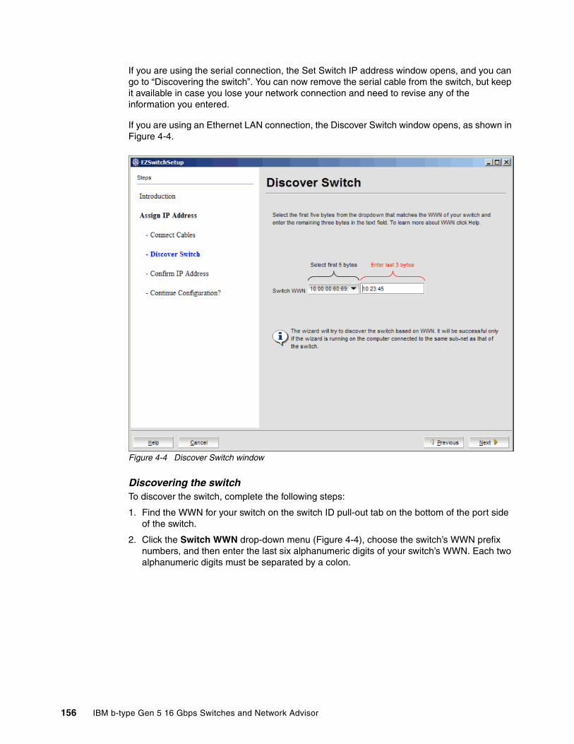
If you are using the serial connection, the Set Switch IP address window opens, and you can go to “Discovering the switch”. You can now remove the serial cable from the switch, but keep it available in case you lose your network connection and need to revise any of the information you entered.
If you are using an Ethernet LAN connection, the Discover Switch window opens, as shown in Figure 4-4.
Figure 4-4 Discover Switch window
Discovering the switchTo discover the switch, complete the following steps:
1. Find the WWN for your switch on the switch ID pull-out tab on the bottom of the port side of the switch.
2. Click the Switch WWN drop-down menu (Figure 4-4), choose the switch’s WWN prefix numbers, and then enter the last six alphanumeric digits of your switch’s WWN. Each two alphanumeric digits must be separated by a colon.
156 IBM b-type Gen 5 16 Gbps Switches and Network Advisor

3. Click Next.
When EZSwitchSetup discovers the switch, it displays the discovered IP addresses (IPv4 and IPv6), as shown in Figure 4-5.
If you are setting up the switch for the first time, the IP addresses are placeholder addresses that were assigned at the factory and you must provide valid addresses.
Figure 4-5 Discover Switch window
Chapter 4. Initial switch setup and configuration 157

4. Select an option for assigning the IP address and click Next. The options vary depending on the configuration of your switch:
– Keep the current switch IP configuration.
This option is available only if EZSwitchSetup detected a valid IP address. Go to “Confirming IP addresses” on page 159.
– Manually assign a static IP address.
If you select this option and click Next, the Set Switch IP address window opens (Figure 4-6). Continue with step 5 to enter the IP address.
– Automatically obtain a valid IPv4 address.
Select this option only if a DHCP server is available on your network. When you click Next, an IP address is automatically obtained from the DHCP server and the Confirm IP address window opens. Go to “Confirming IP addresses” on page 159.
Figure 4-6 Set switch IP address window
5. If you are setting up the switch for the first time, the addresses that are shown are not valid. If you click Next with these addresses in place, EZSwitchSetup returns an error message.
To set up IPv4 addresses, edit the address information in the Set Switch IP address window to create static addresses that are appropriate for your LAN connection.
Note: Starting at step 5, the steps are the same for both serial and Ethernet connections.
158 IBM b-type Gen 5 16 Gbps Switches and Network Advisor

To set up IPv6 addresses, enter the IPv6 address and prefix in the spaces that are provided.
6. Click Next.
EZSwitchSetup attempts to log in using default credentials. If you have changed your admin password, you are prompted to enter your new password.
Confirming IP addressesThe Confirm IP address window (Figure 4-7) opens after you assign IP addresses using either a serial connection or an Ethernet connection.
Figure 4-7 Confirm IP address window
Chapter 4. Initial switch setup and configuration 159
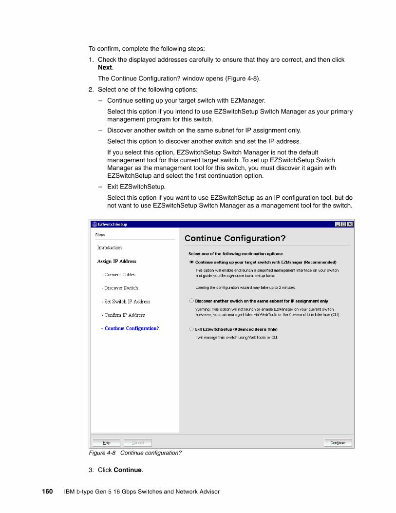
To confirm, complete the following steps:
1. Check the displayed addresses carefully to ensure that they are correct, and then click Next.
The Continue Configuration? window opens (Figure 4-8).
2. Select one of the following options:
– Continue setting up your target switch with EZManager.
Select this option if you intend to use EZSwitchSetup Switch Manager as your primary management program for this switch.
– Discover another switch on the same subnet for IP assignment only.
Select this option to discover another switch and set the IP address.
If you select this option, EZSwitchSetup Switch Manager is not the default management tool for this current target switch. To set up EZSwitchSetup Switch Manager as the management tool for this switch, you must discover it again with EZSwitchSetup and select the first continuation option.
– Exit EZSwitchSetup.
Select this option if you want to use EZSwitchSetup as an IP configuration tool, but do not want to use EZSwitchSetup Switch Manager as a management tool for the switch.
Figure 4-8 Continue configuration?
3. Click Continue.
160 IBM b-type Gen 5 16 Gbps Switches and Network Advisor

Depending on the option that you selected, one of the following outcomes occurs:
� If you selected Continue setting up your target switch with EZManager, a dialog box opens and warns you that EZSwitchSetup supports only single-switch fabrics. Click OK to start the EZSwitchSetup Switch Manager.
A browser window opens, and the Switch Configuration Welcome window opens (Figure 4-9). This process might take a few minutes.
If the EZSwitchSetup switch configuration wizard does not start, you must start it manually by specifying the following URL in a browser:
http://switch-ip-address
� If you selected Discover another switch on the same subnet for IP assignment only, the Discover Switch window opens (Figure 4-4 on page 156). Go to “Discovering the switch” on page 156 and provide the WWN for the next switch.
� If you selected Exit EZSwitchSetup, the EZSwitchSetup switch configuration wizard closes.
Configuring the switchThe EZSwitchSetup switch configuration wizard steps you through the process of changing your administrative password and zoning. You begin at the Welcome to Switch Configuration window, which is shown in Figure 4-9.
Figure 4-9 Welcome to Switch Configuration window
Chapter 4. Initial switch setup and configuration 161

Click Next. The Set Parameters window opens, as shown in Figure 4-10.
Figure 4-10 Set parameters window
Setting switch parametersTo set the switch parameters, complete the following steps:
1. Follow the directions to set a new admin password for the switch. Ensure that you record your password and keep it in a secure location for future reference.
2. Optional: Enter a new name for the switch and set the correct date and time.
3. Click Next. The Select Zoning window opens.
Zoning selection optionsThe next step in configuring your switch is to select zoning. There are three choices:
� Typical Zoning creates a port-based zoning scheme that is based on the connections that are made on the Configure Ports and Connect Devices window. This zoning scheme creates a two-member zone for every possible pairing of HBA (H) and storage (S) ports that are connected, as shown in the Configure Ports and Connect Devices window. This ensures that any host device that is connected to an H port can communicate with any storage device that is connected to an S port.
Note: You can use Typical Zoning for dual-capable devices (devices that are configured to function both as initiators and targets), but in Typical Zoning mode, these devices are recognized as targets by EZSwitchSetup and are rejected if attached to a host port.
162 IBM b-type Gen 5 16 Gbps Switches and Network Advisor

� Custom Zoning allows you to customize which initiators access which targets, and creates a device-based zoning scheme that is based on your choices. The HBAs and storage devices should already be connected to the switch. Custom Zoning provides a device accessibility matrix for you to modify; it then automatically creates zones based on that matrix. Custom Zoning supports only single-switch fabrics. If you select this option, when you click Next, the EZSwitchSetup switch configuration wizard closes and the EZSwitchSetup Switch Manager application opens.
� Advanced Zoning allows you complete customization of your zoning and should be used if you are familiar with zoning and zoning practices. If you select this option, when you click Next, the EZSwitchSetup switch configuration wizard closes and the Advanced Management application (Web Tools) opens. For specific information about using Web Tools for zoning, see the Web Tools Administrator's Guide, which you can find at the following website:
http://my.brocade.com/
Figure 4-11 shows the Select Zoning window.
Figure 4-11 Select Zoning
Typical Zoning is the default and the procedure that is used here assumes that you select Typical Zoning. When you select Typical Zoning, the EZSwitchSetup switch configuration wizard automatically configures the zones for you and shows you how to connect the devices to the switch.
Configuring zones on the switchThese next steps guide you through the Typical Zoning configuration:
1. In the Select Zoning window (Figure 4-11), select Typical Zoning.
2. Click Next.
Chapter 4. Initial switch setup and configuration 163
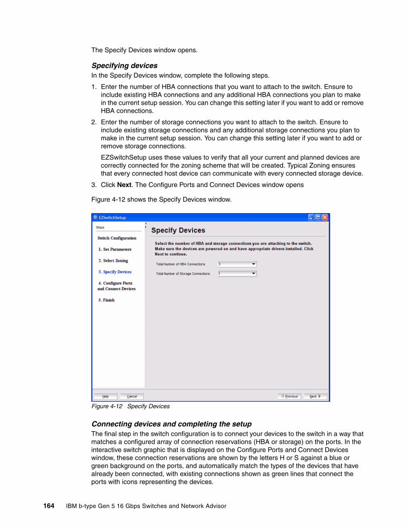
The Specify Devices window opens.
Specifying devicesIn the Specify Devices window, complete the following steps.
1. Enter the number of HBA connections that you want to attach to the switch. Ensure to include existing HBA connections and any additional HBA connections you plan to make in the current setup session. You can change this setting later if you want to add or remove HBA connections.
2. Enter the number of storage connections you want to attach to the switch. Ensure to include existing storage connections and any additional storage connections you plan to make in the current setup session. You can change this setting later if you want to add or remove storage connections.
EZSwitchSetup uses these values to verify that all your current and planned devices are correctly connected for the zoning scheme that will be created. Typical Zoning ensures that every connected host device can communicate with every connected storage device.
3. Click Next. The Configure Ports and Connect Devices window opens
Figure 4-12 shows the Specify Devices window.
Figure 4-12 Specify Devices
Connecting devices and completing the setupThe final step in the switch configuration is to connect your devices to the switch in a way that matches a configured array of connection reservations (HBA or storage) on the ports. In the interactive switch graphic that is displayed on the Configure Ports and Connect Devices window, these connection reservations are shown by the letters H or S against a blue or green background on the ports, and automatically match the types of the devices that have already been connected, with existing connections shown as green lines that connect the ports with icons representing the devices.
164 IBM b-type Gen 5 16 Gbps Switches and Network Advisor
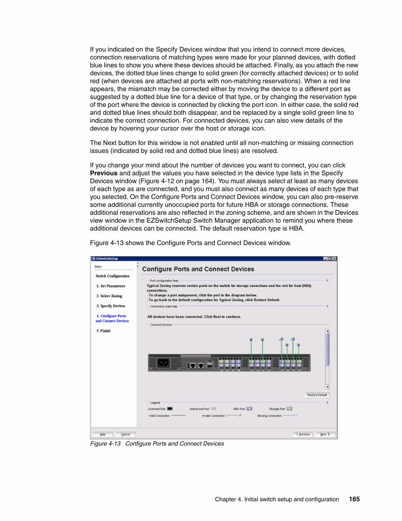
If you indicated on the Specify Devices window that you intend to connect more devices, connection reservations of matching types were made for your planned devices, with dotted blue lines to show you where these devices should be attached. Finally, as you attach the new devices, the dotted blue lines change to solid green (for correctly attached devices) or to solid red (when devices are attached at ports with non-matching reservations). When a red line appears, the mismatch may be corrected either by moving the device to a different port as suggested by a dotted blue line for a device of that type, or by changing the reservation type of the port where the device is connected by clicking the port icon. In either case, the solid red and dotted blue lines should both disappear, and be replaced by a single solid green line to indicate the correct connection. For connected devices, you can also view details of the device by hovering your cursor over the host or storage icon.
The Next button for this window is not enabled until all non-matching or missing connection issues (indicated by solid red and dotted blue lines) are resolved.
If you change your mind about the number of devices you want to connect, you can click Previous and adjust the values you have selected in the device type lists in the Specify Devices window (Figure 4-12 on page 164). You must always select at least as many devices of each type as are connected, and you must also connect as many devices of each type that you selected. On the Configure Ports and Connect Devices window, you can also pre-reserve some additional currently unoccupied ports for future HBA or storage connections. These additional reservations are also reflected in the zoning scheme, and are shown in the Devices view window in the EZSwitchSetup Switch Manager application to remind you where these additional devices can be connected. The default reservation type is HBA.
Figure 4-13 shows the Configure Ports and Connect Devices window.
Figure 4-13 Configure Ports and Connect Devices
Chapter 4. Initial switch setup and configuration 165

When you click Next in the Configure Ports and Connect Devices window, if Typical Zoning is used, the final set of connection reservations that are shown in the window is translated internally into a zoning scheme that ensures that every correctly connected host device can communicate separately with every correctly connected storage device. If this is not what you want (for example, if you want to partition your devices so that each HBA can communicate with some storage devices but not others), then you should rerun the EZSwitchSetup switch configuration wizard and select Custom Zoning or Advanced Zoning instead of Typical Zoning.
After you click Next in the Configuring Ports and Connect Device window, the configuration summary window opens, as shown in Figure 4-14.
Figure 4-14 Finish switch setup window
Click Finish to close the summary window and finish the switch configuration.
166 IBM b-type Gen 5 16 Gbps Switches and Network Advisor
Chapter 5. Gen 5 switches and IBM FlashSystem
This chapter describes how to connect the Gen 5 switches to IBM FlashSystem™ and the IBM SAN Volume Controller.
5
© Copyright IBM Corp. 2014. All rights reserved. 167

5.1 IBM FlashSystem with IBM Gen 5 directors
This section guides you in configuring IBM FlashSystem with IBM Gen 5 directors. It also guides you in virtualizing IBM FlashSystem behind IBM SAN Volume Controller.
The principles and technology that are described in this section are also described in greater depth in Implementing the IBM SAN Volume Controller and FlashSystem 820, SG24-8172.
5.1.1 Introduction to IBM FlashSystem storage systems
IBM FlashSystem storage systems deliver high performance, efficiency, and reliability to various storage environments, helping address performance issues with the most important applications and infrastructure. These storage systems can either complement or replace traditional hard disk drive arrays for many business-critical applications that require high performance or low latency. Such applications include online transaction processing (OLTP), business intelligence (BI), online analytical processing (OLAP), virtual desktop infrastructures (VDIs), high-performance computing (HPC), and content delivery solutions (such as cloud storage and video-on-demand).
Known existing flash-based technologies, such as PCIe flash cards, serial-attached SCSI (SAS), or Serial Advanced Technology Attachment (SATA) solid-state drives (SSDs), are traditionally inside individual servers. Such drives are limited in that they deliver additional performance capability only to the dedicated applications running on the server, and are typically limited in capacity. Hybrid shared storage systems, using both flash and spinning disk technology at the same time, offer the potential to improve performance for a wide range of tasks. However, in products of this type, the internal resources of the system (that is, bus, PCI adapters, and so on) are shared between SSD drives and spinning disks, limiting the performance that can be achieved by using flash technology.
As shared data storage devices that are designed around flash technology, IBM FlashSystem storage systems deliver performance beyond that of most traditional arrays, even those that incorporate SSDs or other flash technology. IBM FlashSystem storage systems can also be used as the top tier of storage, alongside traditional arrays in tiered storage architectures, such as IBM SAN Volume Controller or IBM Storwize® V7000 storage virtualization platforms using the IBM Easy Tier® function. Additionally, IBM FlashSystem storage systems have sophisticated reliability features, such as Variable Stripe Redundant Array of Independent Disks (RAID), which are typically not present on locally attached flash devices.
The IBM FlashSystem portfolio includes shared flash storage systems, SSD devices that are provided in disk storage systems, and server-based flash devices.
For more information, see the IBM FlashSystem home page that is found at the following website:
http://www.ibm.com/systems/storage/flash/
Note: IBM has a rich portfolio of flash-based systems and products. However, for the purposes of this book, we use the term IBM FlashSystem storage systems to refer to the external flash-based systems with Fibre Channel host connectivity only.
168 IBM b-type Gen 5 16 Gbps Switches and Network Advisor
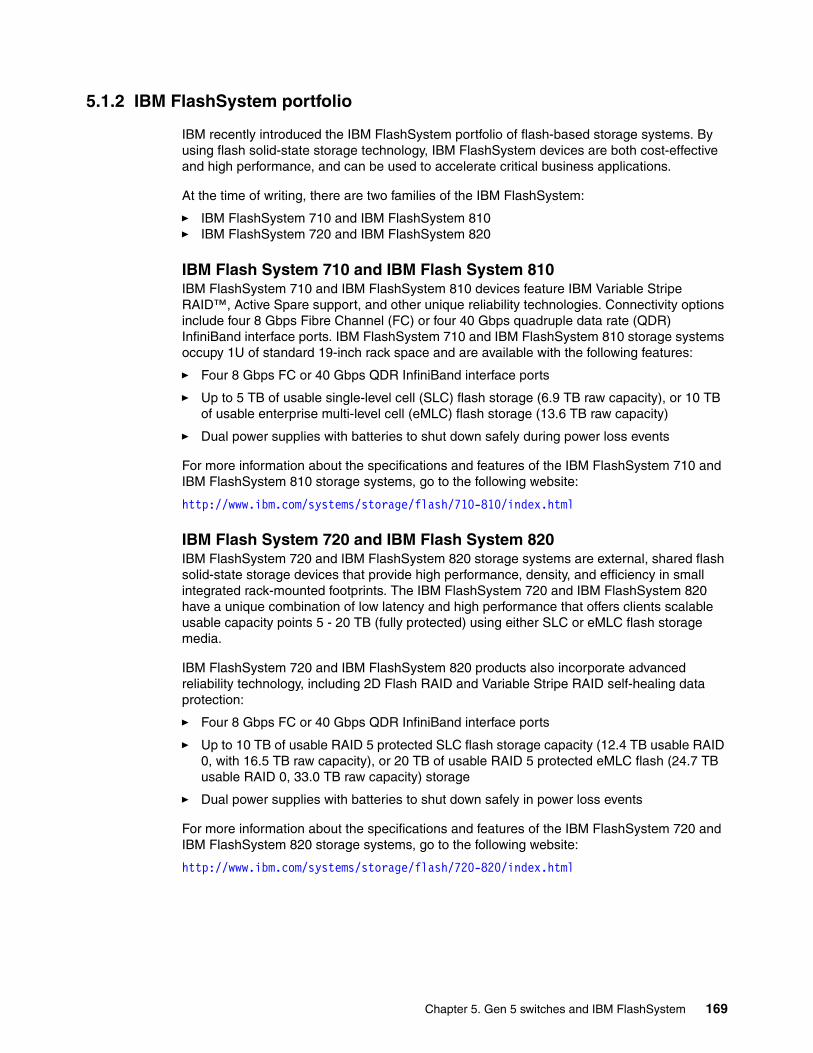
5.1.2 IBM FlashSystem portfolio
IBM recently introduced the IBM FlashSystem portfolio of flash-based storage systems. By using flash solid-state storage technology, IBM FlashSystem devices are both cost-effective and high performance, and can be used to accelerate critical business applications.
At the time of writing, there are two families of the IBM FlashSystem:
� IBM FlashSystem 710 and IBM FlashSystem 810� IBM FlashSystem 720 and IBM FlashSystem 820
IBM Flash System 710 and IBM Flash System 810IBM FlashSystem 710 and IBM FlashSystem 810 devices feature IBM Variable Stripe RAID™, Active Spare support, and other unique reliability technologies. Connectivity options include four 8 Gbps Fibre Channel (FC) or four 40 Gbps quadruple data rate (QDR) InfiniBand interface ports. IBM FlashSystem 710 and IBM FlashSystem 810 storage systems occupy 1U of standard 19-inch rack space and are available with the following features:
� Four 8 Gbps FC or 40 Gbps QDR InfiniBand interface ports
� Up to 5 TB of usable single-level cell (SLC) flash storage (6.9 TB raw capacity), or 10 TB of usable enterprise multi-level cell (eMLC) flash storage (13.6 TB raw capacity)
� Dual power supplies with batteries to shut down safely during power loss events
For more information about the specifications and features of the IBM FlashSystem 710 and IBM FlashSystem 810 storage systems, go to the following website:
http://www.ibm.com/systems/storage/flash/710-810/index.html
IBM Flash System 720 and IBM Flash System 820IBM FlashSystem 720 and IBM FlashSystem 820 storage systems are external, shared flash solid-state storage devices that provide high performance, density, and efficiency in small integrated rack-mounted footprints. The IBM FlashSystem 720 and IBM FlashSystem 820 have a unique combination of low latency and high performance that offers clients scalable usable capacity points 5 - 20 TB (fully protected) using either SLC or eMLC flash storage media.
IBM FlashSystem 720 and IBM FlashSystem 820 products also incorporate advanced reliability technology, including 2D Flash RAID and Variable Stripe RAID self-healing data protection:
� Four 8 Gbps FC or 40 Gbps QDR InfiniBand interface ports
� Up to 10 TB of usable RAID 5 protected SLC flash storage capacity (12.4 TB usable RAID 0, with 16.5 TB raw capacity), or 20 TB of usable RAID 5 protected eMLC flash (24.7 TB usable RAID 0, 33.0 TB raw capacity) storage
� Dual power supplies with batteries to shut down safely in power loss events
For more information about the specifications and features of the IBM FlashSystem 720 and IBM FlashSystem 820 storage systems, go to the following website:
http://www.ibm.com/systems/storage/flash/720-820/index.html
Chapter 5. Gen 5 switches and IBM FlashSystem 169

Advantages of using Gen 5 IBM Director class switches with IBM FlashSystem
These are some of the advantages of combining Gen 5 switches and IBM FlashSystem:
� Unmatched performance, reliability, and scalability� Purpose-built, data center proven network infrastructure for storage � Lowest latency for high-transaction storage� Maximum I/O and bandwidth for application performance� Forward Error Correction (FEC), which is required to bolster reliability and availability� Exploring NPIV (VM) enhancements� Parallel Fibre Channel (128 Gbps) in addition to 32 Gbps Fibre Channel.
5.2 Accessing, connecting, and virtualizing IBM Flash System
This section covers the details about presenting the IBM FlashSystem to the IBM Gen 5 Directors and describes the steps to follow when virtualizing storage with the IBM SAN Volume Controller.
The following topics are described:
� Initial setup of IBM FlashSystem
� Creating logical units on IBM FlashSystem
� Modifying volumes
� Modifying access to the existing volumes
� Port masking and SAN zoning between IBM SAN Volume Controller and IBM FlashSystem
� Creating an MDisk group
5.2.1 Initial setup of IBM FlashSystem
After the IBM FlashSystem is racked, cabled, and powered on, several steps must be performed to configure them optimally for use with IBM SAN Volume Controller. When you configure the IP address for the IBM FlashSystem, the default factory IP address setting of the IBM FlashSystem management controller is Dynamic Host Configuration Protocol (DHCP). In our examples, we use a static IP configuration on Eth0 of the management control processor mc-1, and the second management control processor, mc-2, is not used. Before the IBM FlashSystem is accessible on your network, the LCD display and controls on the front panel of the system should be used to configure the IP address settings.
Initial IP address configuration is explained in greater detail in Implementing the IBM SAN Volume Controller and FlashSystem 820, SG24-8172.
Complete the following steps:
1. To access the IBM FlashSystem remotely, as shown in Figure 5-1 on page 171, use the browser and provide the required details.
170 IBM b-type Gen 5 16 Gbps Switches and Network Advisor
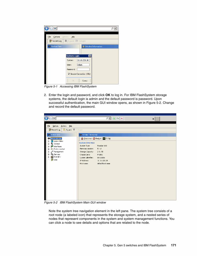
Figure 5-1 Accessing IBM FlashSystem
2. Enter the login and password, and click OK to log in. For IBM FlashSystem storage systems, the default login is admin and the default password is password. Upon successful authentication, the main GUI window opens, as shown in Figure 5-2. Change and record the default password.
Figure 5-2 IBM FlashSystem Main GUI window
Note the system tree navigation element in the left pane. The system tree consists of a root node (a labeled icon) that represents the storage system, and a nested series of nodes that represent components in the system and system management functions. You can click a node to see details and options that are related to the node.
Chapter 5. Gen 5 switches and IBM FlashSystem 171

5.2.2 Creating logical units on IBM FlashSystem
To create a logical unit (LUN), complete the following steps:
1. Click Logical Units in the left pane, and the window shown Figure 5-3 opens.
Figure 5-3 Logical unit creation main window
2. Click Create to continue with creating the volume. As shown in Figure 5-4, a window opens. Read the overview, and click Next to continue.
Figure 5-4 Overview of LUN creation window
3. As shown in Figure 5-5 on page 173, provide all the required details and click Next. Ensure that you select both Report Uncorrected media errors to the SCSI host and Enable ACA support. For more information about the options, go to the following website:
http://www.redbooks.ibm.com/abstracts/tips1003.html
172 IBM b-type Gen 5 16 Gbps Switches and Network Advisor

Figure 5-5 Setup parameters
4. Click Next to continue with the creation of the volume. As shown in Figure 5-6, a confirmation window opens. Select the Confirm above configuration changes check box and click Finish to complete the creation of the LUN.
Figure 5-6 Confirmation window
Chapter 5. Gen 5 switches and IBM FlashSystem 173

5. After you create the volume, as shown in Figure 5-7, the Logical Unit tab on the left pane turns yellow and displays a warning message:
“New volume has no access policy, hence it is not accessible through any controller ports”
Figure 5-7 Logical Unit tab
Select the volume that was created to provide the access through the Fibre Channel ports of the IBM FlashSystem and click Access. The Overview window opens, as shown in Figure 5-8. Click Next to change the access policy for the new volume.
Figure 5-8 Modify Logical Unit Access main window
174 IBM b-type Gen 5 16 Gbps Switches and Network Advisor

6. A window opens, as shown in Figure 5-9. Select the ports through which access should be provided. Select the ports and click the right arrow to move ports from Available to Assigned.
Figure 5-9 Modify Logical Unit Access by selecting ports
7. After you select the ports to provide the access to the new volumes, as shown in Figure 5-10, click Next to continue with the access.
Figure 5-10 Selecting the ports to provide the access to the volumes
Chapter 5. Gen 5 switches and IBM FlashSystem 175
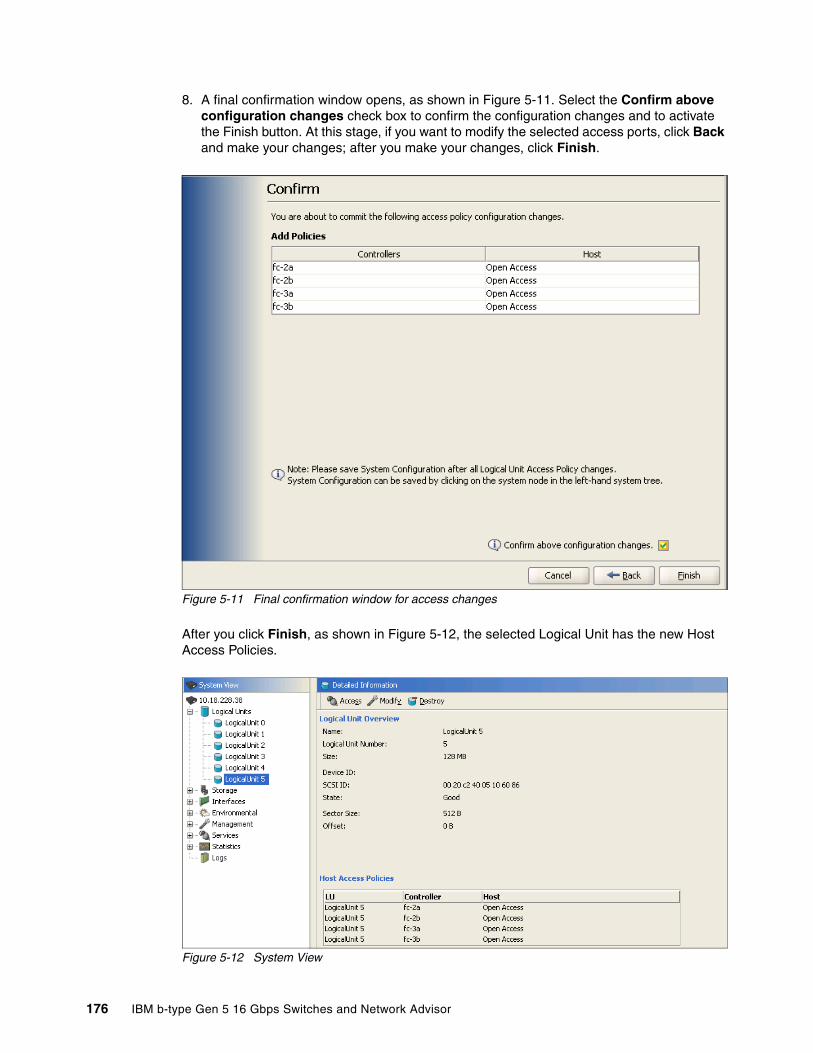
8. A final confirmation window opens, as shown in Figure 5-11. Select the Confirm above configuration changes check box to confirm the configuration changes and to activate the Finish button. At this stage, if you want to modify the selected access ports, click Back and make your changes; after you make your changes, click Finish.
Figure 5-11 Final confirmation window for access changes
After you click Finish, as shown in Figure 5-12, the selected Logical Unit has the new Host Access Policies.
Figure 5-12 System View
176 IBM b-type Gen 5 16 Gbps Switches and Network Advisor

5.2.3 Modifying volumes
To modify the existing volume by adding additional capacity or shrinking capacity, as shown in Figure 5-13, select the volume and click Modify.
Figure 5-13 Change Logical Unit parameters
To expand the existing volume, add the additional amount of space to the existing quantity and select Next.
Chapter 5. Gen 5 switches and IBM FlashSystem 177
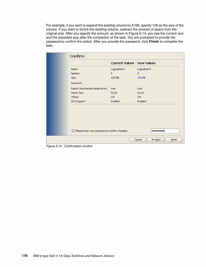
For example, if you want to expand the existing volume by 8 GB, specify 128 as the size of the volume. If you want to shrink the existing volume, subtract the amount of space from the original size. After you specify the amount, as shown in Figure 5-14, you see the current size and the expected size after the completion of the task. You are prompted to provide the password to confirm the action. After you provide the password, click Finish to complete the task.
Figure 5-14 Confirmation window
178 IBM b-type Gen 5 16 Gbps Switches and Network Advisor
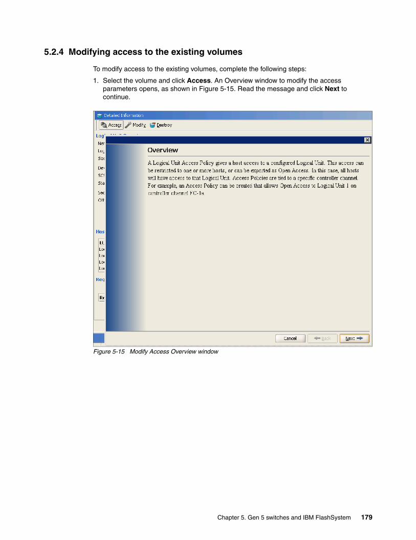
5.2.4 Modifying access to the existing volumes
To modify access to the existing volumes, complete the following steps:
1. Select the volume and click Access. An Overview window to modify the access parameters opens, as shown in Figure 5-15. Read the message and click Next to continue.
Figure 5-15 Modify Access Overview window
Chapter 5. Gen 5 switches and IBM FlashSystem 179

2. A window with the Modify Access parameters opens, as shown in Figure 5-16. Click the controller ports for which you want to add / remove access, select the correct arrow, and click Next.
Figure 5-16 Modifying Access
3. After you select the controller port, click Next to continue. Confirmation is required to continue with the addition or removal of access ports, as shown in Figure 5-17 on page 181. After you provide the password, click Finish to complete the task.
180 IBM b-type Gen 5 16 Gbps Switches and Network Advisor
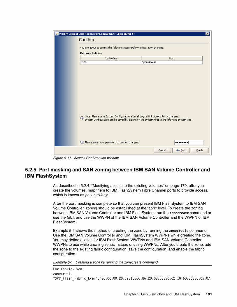
Figure 5-17 Access Confirmation window
5.2.5 Port masking and SAN zoning between IBM SAN Volume Controller and IBM FlashSystem
As described in 5.2.4, “Modifying access to the existing volumes” on page 179, after you create the volumes, map them to IBM FlashSystem Fibre Channel ports to provide access, which is known as port masking.
After the port masking is complete so that you can present IBM FlashSystem to IBM SAN Volume Controller, zoning should be established at the fabric level. To create the zoning between IBM SAN Volume Controller and IBM FlashSystem, run the zonecreate command or use the GUI, and use the WWPN of the IBM SAN Volume Controller and the WWPN of IBM FlashSystem.
Example 5-1 shows the method of creating the zone by running the zonecreate command. Use the IBM SAN Volume Controller and IBM FlashSystem WWPNs while creating the zone. You may define aliases for IBM FlashSystem WWPNs and IBM SAN Volume Controller WWPNs to use while creating zones instead of using WWPNs. After you create the zone, add the zone to the existing fabric configuration, save the configuration, and enable the fabric configuration.
Example 5-1 Creating a zone by running the zonecreate command
For Fabric-Evenzonecreate "SVC_Flash_Fabric_Even","20:0c:00:20:c2:10:60:86;20:08:00:20:c2:10:60:86;50:05:07:
Chapter 5. Gen 5 switches and IBM FlashSystem 181
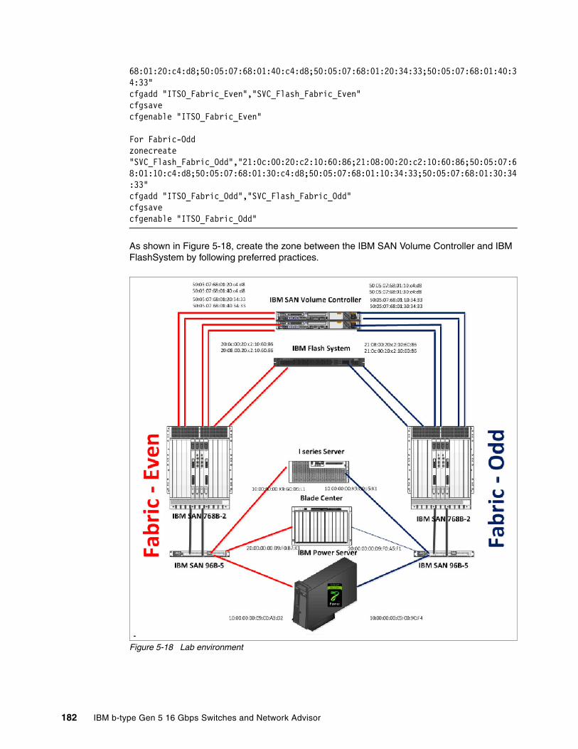
68:01:20:c4:d8;50:05:07:68:01:40:c4:d8;50:05:07:68:01:20:34:33;50:05:07:68:01:40:34:33"cfgadd "ITSO_Fabric_Even","SVC_Flash_Fabric_Even"cfgsavecfgenable "ITSO_Fabric_Even"
For Fabric-Oddzonecreate "SVC_Flash_Fabric_Odd","21:0c:00:20:c2:10:60:86;21:08:00:20:c2:10:60:86;50:05:07:68:01:10:c4:d8;50:05:07:68:01:30:c4:d8;50:05:07:68:01:10:34:33;50:05:07:68:01:30:34:33"cfgadd "ITSO_Fabric_Odd","SVC_Flash_Fabric_Odd"cfgsavecfgenable "ITSO_Fabric_Odd"
As shown in Figure 5-18, create the zone between the IBM SAN Volume Controller and IBM FlashSystem by following preferred practices.
Figure 5-18 Lab environment
182 IBM b-type Gen 5 16 Gbps Switches and Network Advisor

For more information about how to create zones, go to the following website:
http://www.brocade.com/downloads/documents/product_manuals/B_SAN/FOS_AdminGd_v700.pdf
Example 5-2 describes the zoning information from our test environment (shown in Figure 5-18 on page 182) for both fabrics.
In Figure 5-18 on page 182, you can see two fabrics, “Fabric-Even” and “Fabric-Odd”. Fabric-Even contains one IBM System Networking SAN 768B-2 director class switch and one IBM System Networking SAN 96B-5 switch. Fabric-Odd contains one SAN 768B-2 director class switch and one SAN 96B-5. Both fabrics are designed for a “Core-Edge” topology, where IBM FlashSystem and IBM SAN Volume Controller are connected into the SAN768B-2 director class switch and the hosts are connected into the SAN 96B-5 switch. In the current environment, IBM FlashSystem even-numbered ports are connected into Fabric-Even and the odd-numbered ports are connected into the Fabric-Odd.
As shown in Example 5-2, in our example environment, we create the zone between the even ports of IBM FlashSystem and IBM SAN Volume Controller, and between the odd ports of IBM FlashSystem and IBM SAN Volume Controller.
Example 5-2 Zoning information from our test environment
Zone information from Fabric-Evenzone: SVC_Flash_Fabric_Even 20:0c:00:20:c2:10:60:86 20:08:00:20:c2:10:60:86 50:05:07:68:01:20:c4:d8 50:05:07:68:01:40:c4:d8 50:05:07:68:01:20:34:33 50:05:07:68:01:40:34:33Zone information from Fabric-Oddzone: SVC_Flash_Fabric_Odd 21:08:00:20:c2:10:60:86 21:0c:00:20:c2:10:60:86 50:05:07:68:01:30:34:33 50:05:07:68:01:10:34:33 50:05:07:68:01:10:c4:d8 50:05:07:68:01:30:c4:d8
5.2.6 Creating an MDisk group
As mentioned earlier, after you complete the port masking at the IBM FlashSystem level and zoning at the fabric level, log in to the IBM SAN Volume Controller to create an MDisk group. To list the newly added MDisks from IBM FlashSystem, run lsmdisk. If no disks are displayed, run detectmdisk to detect the newly added volumes.
Example 5-3 lists the newly presented MDisks from IBM FlashSystem to IBM SAN Volume Controller.
Example 5-3 Newly presented MDisks to IBM SAN Volume Controller
IBM_2145:ITSO_Redbooks:admin>lsmdiskid name status mode mdisk_grp_id mdisk_grp_name capacity ctrl_LUN_# controller_name UID tier
Chapter 5. Gen 5 switches and IBM FlashSystem 183

0 mdisk0 online unmanaged 120.0GB 0000000000000000 FlashSystem 0020c24000106086000000000000000000000000000000000000000000000000 generic_hdd1 mdisk4 online unmanaged 120.0GB 0000000000000001 FlashSystem 0020c24001106086000000000000000000000000000000000000000000000000 generic_hdd2 mdisk2 online unmanaged 120.0GB 0000000000000002 FlashSystem 0020c24002106086000000000000000000000000000000000000000000000000 generic_hdd3 mdisk3 online unmanaged 120.0GB 0000000000000003 FlashSystem 0020c24003106086000000000000000000000000000000000000000000000000 generic_hdd4 mdisk1 online unmanaged 120.0GB 0000000000000004 FlashSystem 0020c24004106086000000000000000000000000000000000000000000000000 generic_hddIBM_2145:ITSO_Redbooks:admin>
After you present the new MDisks, create an MDisk group to add the MDisks. Example 5-4 describes the process of creating an MDisk group by using the newly presented MDisks.
Example 5-4 Creating an MDisk group on IBM SAN Volume Controller
IBM_2145:ITSO_Redbooks:admin>mkmdiskgrp -name Flash_System -mdisk mdisk0:mdisk1:mdisk2:mdisk3:mdisk4 -ext 1024MDisk Group, id [0], successfully createdIBM_2145:ITSO_Redbooks:admin>lsmdiskgrpid name status mdisk_count vdisk_count capacity extent_size free_capacity virtual_capacity used_capacity real_capacity overallocation warning easy_tier easy_tier_status compression_active compression_virtual_capacity compression_compressed_capacity compression_uncompressed_capacity0 Flash_System online 5 0 597.00GB 1024 597.00GB 0.00MB 0.00MB 0.00MB 0 0 auto inactive no 0.00MB 0.00MB 0.00MBIBM_2145:ITSO_Redbooks:admin>lsmdiskid name status mode mdisk_grp_id mdisk_grp_name capacity ctrl_LUN_# controller_name UID tier0 mdisk0 online managed 0 Flash_System 120.0GB 0000000000000000 FlashSystem 0020c24000106086000000000000000000000000000000000000000000000000 generic_hdd1 mdisk4 online managed 0 Flash_System 120.0GB 0000000000000001 FlashSystem 0020c24001106086000000000000000000000000000000000000000000000000 generic_hdd2 mdisk2 online managed 0 Flash_System 120.0GB 0000000000000002 FlashSystem 0020c24002106086000000000000000000000000000000000000000000000000 generic_hdd3 mdisk3 online managed 0 Flash_System 120.0GB 0000000000000003 FlashSystem 0020c24003106086000000000000000000000000000000000000000000000000 generic_hdd4 mdisk1 online managed 0 Flash_System 120.0GB 0000000000000004 FlashSystem 0020c24004106086000000000000000000000000000000000000000000000000 generic_hddIBM_2145:ITSO_Redbooks:admin>
184 IBM b-type Gen 5 16 Gbps Switches and Network Advisor

For more information and greater depth about IBM SAN Volume Controller and IBM FlashSystem, see Implementing the IBM SAN Volume Controller and FlashSystem 820, SG24-8172.
Chapter 5. Gen 5 switches and IBM FlashSystem 185

186 IBM b-type Gen 5 16 Gbps Switches and Network Advisor

Chapter 6. Preferred practices
This chapter is a high-level design and preferred practices guide that is based on IBM b-type Gen 5 16 Gbps products and features, focusing on Fibre Channel SAN design. The topics include the early planning phase, topologies, understanding possible operational challenges, and monitoring and improving a SAN infrastructure that is already implemented. The guidelines in this chapter do not apply to every environment, but can guide you through the decisions that you must make for a successful SAN design.
6
© Copyright IBM Corp. 2014. All rights reserved. 187
6.1 Physical patching
Today’s data centers house many diverse bandwidth-intensive devices, including bladed servers, clustered storage systems, virtualization appliances, and backup devices, all of which are interconnected by networking equipment. These devices require physical cabling with an increasing demand for higher performance and flexibility, all of which require a reliable, scalable, and manageable cabling infrastructure.
Challenges arise not only with trying to research emerging data center cabling offerings to determine what you need for today and for future growth, but also with evolving cabling industry guidance, which sometimes lags in the race to deliver standards for deploying technologies such as 16 Gbps data transmissions.
The next sections describe some of the cabling preferred practices and guidelines. Other components, such as cooling, power, and space capacity that involves data center manageability are not within the intended scope of this book.
6.1.1 Using a structured approach
The structured approach to cabling involves designing cable runs and connections to facilitate the identification of cables, troubleshooting, and planning for future changes. In contrast, spontaneous or reactive deployment of cables to suit immediate needs often makes it difficult to diagnose problems and to verify correct connectivity.
Using a structured approach means establishing a Main Distribution Area (MDA), one or several Horizontal Distribution Areas (HDAs), and two-post racks for better access and cable management. The components that are selected for building the MDA and the HDA should be of good quality and able to handle anticipated and future loads, as this area houses the bulk of the cabling. Include horizontal and vertical cable managers in the layout. The MDA houses the main cross-connects and the core networking equipment. The HDA houses the cross-connects for distributing cables to the Equipment Distribution Areas (EDAs). Patch cables are used to connect equipment, such as servers and storage, by using the patch panels at their designated EDA.
Plan the layout of the equipment racks within the data center. Cables are distributed from the HDA to the EDA by using horizontal cabling. Ensure that you address both current and future port counts and applications needs.
Each scenario has its own challenges and customization requirements. It is important to read the TIA-942 and the TIA/EIA-568 industry guidelines and to establish a structure for the cabling. Each cabling component has an important role in the overall infrastructure, you must carefully select and apply the correct structure.
Structuring the cabling has many benefits, and because manufacturers strive to conform to standards, compatibility should not be a major issue. A structured infrastructure provides you with some of the following benefits:
� Simplifies cable identification and fault isolation.
� Consistent current cabling shapes the foundation for future cabling.
� Additions and modifications are easier to accommodate.
� You can mix-and-match multivendor components (ensure that they comply with the same standards).
� Provides flexibility in connections.
188 IBM b-type Gen 5 16 Gbps Switches and Network Advisor

6.1.2 Modular cabling
Modular cabling systems for fiber and copper connectivity are becoming more prevalent. Modular cabling introduces the concept of plug-and-play, which simplifies the installation of cables and drastically reduces labor time and costs. Cables are usually pre-terminated and tested at the factory.
As equipment prices continue to drop, vendors continue to build better options. The main difference to consider currently is the cost of modular components versus the cost of labor for a non-modular but structured offering. Although modular cabling saves you time and money when you want to modify the infrastructure yourself, the trade-off is less flexibility and a potential commitment to stay with the chosen vendor for continued compatibility.
6.1.3 Cabling high-density and high-port count fiber equipment
As networking equipment becomes denser and port counts in the data center increase to several hundred ports, managing cables that are connected to these devices becomes a difficult challenge. Traditionally, connecting cables directly to individual ports on low-port-count equipment was considered manageable. Applying the same principles to high-density and high-port-count equipment makes the task more tedious, and it is nearly impossible to add or remove cables that are connected directly to the equipment ports.
Using fiber cable assemblies that have a single connector at one end of the cable and multiple duplex breakout cables at the other end is an alternative to alleviate cable management. Multifiber Push-On (MPO) cable assemblies can achieve these goals. The idea is to pre-connect the high-density and high-port- count Lucent Connector (LC) equipment with an LC-MPO fan-out cable (shown in Figure 6-1) to dedicated MPO modules within a dedicated patch panel. After the panel is fully cabled, this patch panel functions as though it were “remote” ports for the equipment. These dedicated patch panels ideally should be above the equipment whose cabling they handle for easier access to overhead cabling. Using this strategy drastically reduces equipment cabling clutter and improves cable management.
Figure 6-1 An LC-MPO fan-out cable consolidates six duplex LC ports into one MPO connection
Chapter 6. Preferred practices 189

As an example, the MPO module that is shown in Figure 6-1 on page 189 is housed in a modular patch panel that is installed above a Fibre Channel director switch at the EDA. MPO trunk cables are used to link this patch panel to another modular patch panel at the HDA. The patch panel at the HDA converts the MPO interface back to the LC interfaces by using MPO-to-LC cassettes. MPO trunk cables can accommodate up to 72 individual fibers in one assembly, providing 36 duplex connections.
6.1.4 Using color to identify cables
Color provides quick visual identification. Color coding simplifies management and can save you hours when you need to trace cables. Color coding can be applied to ports on a patch panel. Patch panels themselves come with different color jacks or have colored inserts that surround the jack. Cables are available in many colors (the color palette depends on the cable manufacturer). Apply these colors to identify the role/function of a cable or the type of connection. Table 6-1 is an example color scheme for patch cables.
Table 6-1 Example of a color scheme for patch cables
In addition to cable colors, you can expand the color scheme by using different 1-inch color bands at each end of the cable, different color sleeves, and different color ports on the patch panel.
If you use colors to identify cable functions or connections, build in redundancy to accommodate individuals with color blindness or color vision deficiency.
6.1.5 Establishing a naming scheme
AFter the logical and physical layouts for the cabling are defined, apply logical naming that uniquely and easily identifies each cabling component. Effective labeling promotes better communications and eliminates confusion when someone is trying to find a component. Labeling is a key part of the process and should not be skipped. A suggested naming scheme for labeling and documenting cable components is suggested here (examples appear in parentheses):
� Building (CA01)
� Room (CA01-4R22)
� Rack or Grid Cell: Can be a grid allocation within the room (CA01-4R22-A04)
� Patch Panel: Instance in the rack or area (CA01-4R22-A04-PP03)
� Port: Instance in the patch panel or workstation outlet (CA01-4R22-A04-PP03_01)
� Cable (each end labeled with the destination port)
You can exclude Building and Room if there is only one instance of this entity in your environment.
After the naming scheme is approved, you can start labeling the components. Create a reference document that becomes part of the training for new data center administrators.
Color Type Application (connections may be through patch panels)
Orange OM1 or OM2 fiber SAN device to device
Aqua OM3 fiber SAN device to device
Yellow Single Mode Fiber LAN/SAN device to device over long distance
190 IBM b-type Gen 5 16 Gbps Switches and Network Advisor

6.1.6 Patch cables
Patch cables are used to connect devices to patch panel ports and to connect ports between two local patch panels. A significant issue with patch cables is the design and quality of the terminations. The patch cable is the cabling component that experiences the most wear and tear.
6.1.7 Patch panels
Patch panels allow the easy management of patch cables and link the cabling distribution areas. The preferred practice is to separate the fiber cabling from the copper cabling by using separate patch panels, although mixing cable types with the same patch panel is an option through multimedia patch panels.
Colored jacks or bezels in the patch panel allow easy identification of the ports and the applications they are intended for. Patch panels also come in modular styles, for example, for an MPO structured system. The trade-off for the higher cost of materials is that some of this cost is recovered from faster installation and lower labor costs.
6.1.8 Horizontal and backbone cables
Choose the fire-rated plenum type. These cables might not be as flexible as the patch cords because they are meant for fairly static placements, for example, between the EDA and the HDA. For fiber, high density involving 24-strand to 96-strand cables is adequate. Fiber breakout cables provide more protection, but add to the diameter of the overall cable bundle. For fiber, MPO trunk cables (up to 72 fiber strands can be housed in one MPO connection) can be installed if you are using MPO style cabling.
Evaluate the cost of materials and labor for terminating connections into patch panels. These cables will most likely end up under raised floors, or over the ceiling, or in overhead cable pathways out of view and touch from users.
6.1.9 Horizontal cable managers
Horizontal cable managers allow the neat and correct routing of the patch cables from equipment in racks and protect cables from damage. These cable managers take up the much-needed space in racks, so a careful balance between cable manager height and cable density is important. 1U and 2U horizontal cable managers are the most common varieties. The density that is supported varies with the height and depth of the manager. Horizontal cable managers come in metal and flexible plastic; choose the ones that work best for you. The ideal cable manager has a large enough lip to easily position and remove cables, and has sufficient depth to accommodate the quantity of cables that are planned for that area. You should allow 30% additional space in the cable managers for future growth.
Choose these cable managers carefully so that the cable bend radius is accommodated. Make sure that certain parts of the horizontal cable manager are not obstructing equipment in the racks, and that those individual cables are easy to add and remove. Some cable managers come with dust covers. For dynamic environments, however, dust covers can be an obstacle when quick cable changes are required.
Chapter 6. Preferred practices 191

6.1.10 Vertical cable managers
For vertical cable managers, look for the additional space that is required to manage the slack from patch cords, and ensure that they can easily route the largest cable diameter in your plan. The most convenient managers available on the market have hinged doors on both sides of the manager for pivoting the door from either side, and allow complete removal of the doors for unobstructed access.
Allow for 50% growth of cables when planning the width (4-inch width for edge racks and 6-inch width for distribution racks are typical) and depth (6-inch depth is typical) of the vertical cable manager. Additionally, use d-rings type cable managers to manage cables on the back side of the racks in dynamic environments. For static environments, you can consider installing another vertical cable manager behind the racks, which does not block access to components in the space between the racks.
6.1.11 Overhead cable pathways
Overhead cable pathways or trays allow placement of more cables for interconnecting devices between racks on an ad hoc basis. Check support for cable bend radius, weight allowance, sagging points for cables, and flexibility in installing the pathways. In addition, ensure that pathways allow cable drop points where needed. These trays should be easy to install and to customize.
6.1.12 Cable ties
Use cable ties to hold a group of cables together or to fasten cables to other components. Choose Hook-and-loop fastener-based cable ties versus zip ties, as there is a tendency for users to over-tighten zip ties. Overtightening can crush the cables and impact performance. Hook-and-loop fastener cable ties come in a roll or in predetermined lengths. Bundle groups of relevant cables with ties as you install, which helps you identify cables later and facilitate better overall cable management.
6.1.13 Implementing the cabling infrastructure
The cabling infrastructure is under a raised floor, overhead, or both. This is where the bulk of the horizontal cabling is installed. Most likely, you will hire a reputable cabling contractor to survey the environment, plan out the cabling routes, and install the horizontal runs. Ensure that copper and fiber runs are separated because the weight of copper cables can damage the fiber.
6.1.14 Testing the links
Testing cables throughout the installation stage is imperative. Any cables that are relocated or terminated after testing should be retested. Although testing is carried out by an authorized cabling implementor, you should obtain a test report for each cable that is installed as part of the implementation task.
192 IBM b-type Gen 5 16 Gbps Switches and Network Advisor

6.1.15 Building a common framework for the racks
The goal of this task is to stage a layout that can be mirrored across all racks in the data center for consistency, management, and convenience. Starting with an empty 4-post rack or two, build and establish an internal standard for placing patch panels, horizontal cable managers, vertical cable managers, power strips, a KVM switch, serial console switch, and any other devices that are planned for placement in to racks or a group of racks. The idea is to fully cable the common components while monitoring the cooling, power, equipment access, and growth for the main components in the racks (such as servers and network switches).
Figure 6-2 shows front and back view of a rack, which shows placements of common cabling components.
Figure 6-2 Rack example with common components
A good layout discourages cabling in between racks because of the lack of available data ports or power supply ports. Allow more power outlets and network ports than you need, which saves you money in the end as rack density increases, calling for more power and network connectivity. Using correct length cables, route patch cables up or down through horizontal patch panels, while avoiding overlapping other ports. Some cable slack might be needed to enable easy removal of racked equipment.
After you are satisfied that the rack is populated and cabled efficiently, label, document, and establish this rack as an internal standard for your data center. After you create the ideal layout of a rack, you get an idea of cable density, power consumption, weight, and the heat that is generated per rack for the entire data center. The actual figures vary from rack to rack, but this ideal rack establishes baseline metrics.
Chapter 6. Preferred practices 193
Vertical cable managers should be mounted between racks. The outermost rack might not need a vertical cable manager if you decide to route cables by using the between-rack vertical cable managers only. Also, ensure that the front of the vertical cable manager is flush with the front of the horizontal cable manager to provide better routing and management of the cables.
Placement of horizontal cable managers is important. Use one horizontal cable manager to route cables between two adjacent 1U switches that have a single row of ports. For switches and equipment that have two rows of ports, route the cables from the top row of the equipment to a horizontal cable manager placed above this equipment, and route the cables from the bottom row of the equipment to a horizontal cable manager placed below the equipment.
6.1.16 Preserving the infrastructure
Physically, the cabling infrastructure is at its “peak” immediately following a clean installation or upgrade. Even when you hired a cabling contractor to install, label, dress, and test the cabling, when the contractor walks away, it is your task to manage and maintain the conventions that you set up initially.
Regular inspections of the cabling layout go a long way toward maintaining consistency. They also help you identify problem areas for improvement and give you ideas for future enhancements to accommodate newer devices.
6.1.17 Documentation
Perhaps the most critical task in cable management is to document the complete infrastructure, which should include diagrams, cable types, patching information, and cable counts.
The cabling contractor should provide this documentation, so ensure that you keep this information easily accessible to data center staff. Assign updates to one or more staff members and make sure that it is part of their job assignment to keep the documentation up-to-date. Furthermore, create a training guide that documents guidelines for installing cables, cable management components, and routing cables. Take digital photographs as reference points to support your guiding principles.
6.1.18 Stocking spare cables
Where do you go when you need the correct type and correct length patch cable right away? Unless you are good with cable terminating tools, buy a small stock of cables in multiple lengths and colors. The most frequently used patch cable lengths are 3 ft, 5 ft, and 7 ft. The types and colors vary per implementation. The variation that is most common to your environment is self-evident after you have fully cabled two to three racks in the data center. Although in an emergency there is a human tendency to “cannibalize” existing equipment that is not being used, this is not a preferred practice.
Maintaining an approximate count on the installed cabling and port count usage gives you an idea of what spares you need to have available. Paradoxically, managing spare cables has its own challenges. How do you effectively store and easily identify recoiled cables, and keep a count of the spares? Again, discipline is the key, with whatever guidelines you have in place.
194 IBM b-type Gen 5 16 Gbps Switches and Network Advisor

6.1.19 Preferred practices for managing cabling
Whether you implement, upgrade, or maintain cabling in the data center, establish a set of guidelines that are thoroughly understood and supported by the staff. This section has some pointers for managing your cabling.
During installationDuring the installation of your cabling, follow these preferred practices:
� Avoid over-bundling the cables or placing multiple bundles on top of each other, which can degrade the performance of the cables underneath. Additionally, keep fiber and copper runs separated because the weight of the copper cables can crush any fiber cables that are placed underneath.
� Avoid mounting cabling components in locations that block access to other equipment inside and outside the racks.
� Keep all cable runs under 90% of the maximum distance that is supported for each media type as specified in the relevant standard. This extra headroom is for the additional patch cables that are included in the end-to-end connection.
� For backbone and horizontal runs, install additional cables as spares.
� Cabling installations and components should be compliant with industry standards.
� Do not stress the cable by doing any of the following actions:
– Applying additional twists
– Pulling or stretching beyond the cable’s specified pulling load rating
– Bending the cable beyond its specified bend radius, and not beyond 90º
– Creating tension in suspended runs
– Stapling or applying pressure with cable ties
� Avoid routing cables through pipes and holes, which might limit additional future cable runs.
� Label cables with their destination at every termination point (this means labeling both ends of the cable).
� Test every cable as it is installed and terminated. It is difficult to identify problem cables later.
� Place the main cabling distribution area nearer the center of the data center to limit cable distances.
� Dedicate outlets for terminating horizontal cables, that is, allocate a port in the patch panel for each horizontal run.
� Include sufficient vertical and horizontal managers in your design; future changes might involve downtime as cables are removed during the changes.
� Use angled patch panels within high-density areas, such as the cable distribution area. Use straight patch panels at the distribution racks.
� Use modular cabling systems to map ports from equipment with high-density port counts, as described in 6.1.1, “Using a structured approach” on page 188.
Chapter 6. Preferred practices 195

Daily practicesFollow these daily practices:
� Avoid leaving loose cables on the floor; this is a major safety hazard. Use the horizontal, vertical, or overhead cable managers.
� Avoid exposing cables to direct sunlight and areas of condensation.
� Do not mix 50-micron cables with 62.5-micron cables on a link.
� Remove abandoned cables that can restrict air flow and potentially fuel a fire.
� Keep some spare patch cables. The types and quantity can be determined from the installation and projected growth. Try to keep all unused cables bagged and capped when not in use.
� Use horizontal and vertical cable guides to route cables within and between racks. Use “cable spool” devices in cable managers to avoid kinks and sharp bends in the cable.
� Document all cabling components and their linkage between components and make sure that this information is updated on a regular basis. The installation, labeling, and documentation should always match.
� Use the correct length patch cable, leaving some slack at each end for device movements.
� Bundle cables together in groups of relevance (for example, ISL cables and uplinks to core devices), as this eases management and troubleshooting.
� When bundling or securing cables, use hook-and-loop fastener-based ties every 12 - 24 inches. Avoid using zip ties, as these apply pressure on the cables.
� Avoid routing cables over equipment and other patch panel ports. Route below or above and into the horizontal cable manager for every cable.
� Maintain the cabling documentation, labeling, and logical/physical cabling diagrams.
� Maintain a small stock of the most commonly used patch cables.
6.1.20 Summary
Although cabling represents less than 10% of the overall data center network investment, expect it to outlive most other network components and expect it to be the most difficult and potentially costly component to replace. When you purchase the cabling infrastructure, consider not only the initial implementation costs, but subsequent costs as well. Understand the full lifecycle and study local industry trends to arrive at the correct decision for your environment.
Choose the strongest foundation to support your present and future network technology needs and comply with TIA/ISO cabling standards. The cabling itself calls for the correct knowledge, the correct tools, patience, a structured approach, and most of all, discipline. Without discipline, it is common to see complex cabling “masterpieces” quickly get out of control, leading to chaos.
Because each environment is different, there is no single solution that meets all of your cable management needs. Following the guidelines and preferred practices that are presented here goes a long way to providing you with the information that is required for the successful deployment of a cabling infrastructure in your data center.
196 IBM b-type Gen 5 16 Gbps Switches and Network Advisor
6.2 SAN design basics
This section focus on preferred practices for core-edge or edge-core-edge fabrics. It describes the concepts of topology, Inter-Switch Links, Inter-Chassis Links, device placement, and oversubscription.
6.2.1 Topologies
A typical SAN design has devices on the edge of the network, switches in the core of the network, and the cabling that connects it all together. Topology is described in terms of how the switches are interconnected, such as ring, core-edge, and edge-core-edge or fully meshed. At this point, the focus is on switch topology with ISLs. The recommended SAN topology to optimize performance, management, and scalability is a tiered, core-edge topology (sometimes called core-edge or tiered core-edge). This approach provides good performance without unnecessary interconnections. At a high level, the tiered topology has many edge switches that are used for device connectivity, and fewer core switches that are used for routing traffic between the edge switches.
An important aspect of SAN topology is the resiliency and redundancy of the fabric. The main objective is to remove any single point of failure. Resiliency is the ability of the network to continue to function or recover from a failure, and redundancy describes duplication of components, even an entire fabric, to eliminate a single point of failure in the network. Brocade fabrics have resiliency built into Brocade FOS, the software that runs on all Brocade B-Series switches, which can quickly “repair” the network to overcome most failures. For example, when a link between switches fails, Fabric Shortest Path First (FSPF) quickly recalculates all traffic flows. This assumes that there is a second route, which is when redundancy in the fabric becomes important.
The key to high availability and enterprise-class installation is redundancy. By eliminating a single point of failure, business continuance can be provided through most foreseeable and even unforeseeable events. At the highest level of fabric design, the complete network should be redundant, with two separate fabrics that do not share any network equipment (routers or switches).
Preferred practicesHere some preferred practices for setting up SAN topologies:
� Use two core switches instead of a single one in core-edge and edge-core-edge designs. This configuration improves resilience in the fabric and avoids host failovers to alternative fabrics in case a core platform ever fails. Experience has shown that host failover software sometimes does not function as expected, causing outages for applications that were expected to participate in a host failover to a second fabric.
� Duplicate the Fibre Channel Router (FCR) backbone switches to protect against host failover failures. Often, the costs that are associated with a failover failure exceed the cost of the second FCR platform.
� Provide as many different paths through the fabric as possible, especially for routed fabrics, as these are prime points of congestion.
6.2.2 Inter-Switch Link
An Inter-switch Link (ISL) is a link between two switches (referred to as E_Ports). ISLs carry frames originating from the node ports, and those generated within the fabric. The frames that are generated within the fabric serve as control, management, and support for the fabric.
Chapter 6. Preferred practices 197
To maximize the performance of your ISLs, implement trunking. This technology is ideal for optimizing performance and simplifying the management of multi-switch SAN fabrics. When two or more adjacent ISLs in a port group are used to connect two switches with trunking enabled, the switches automatically group the ISLs into a single logical ISL, or trunk.
ISL Trunking reduces traffic congestion in storage networks. To balance the workload across all of the ISLs in the trunk, each incoming frame is sent across the first available physical ISL in the trunk. As a result, transient workload peaks are much less likely to impact the performance of other parts of the SAN fabric and bandwidth is not wasted by inefficient traffic routing. ISL Trunking can also help simplify fabric design, lower provisioning time, and limit the need for additional ISLs or switches.
To further optimize network performance, b-type switches and directors support Exchange-based routing, which is also known as Dynamic Path Selection (DPS). Available as a standard feature in FOS (starting in FOS V4.4), DPS optimizes fabric-wide performance by automatically routing data to the most efficient available path in the fabric. DPS augments ISL Trunking to provide more effective load balancing in certain configurations, such as routing data between multiple trunk groups.
As a preferred practice, there should be a minimum of two trunks, with at least two ISLs per trunk. DLS should be used to provide more effective load balancing, such as routing between multiple trunk groups.
6.2.3 Inter-Chassis Links
Inter-Chassis Links (ICLs) are high-performance ports for interconnecting multiple backbones, enabling industry-leading scalability while preserving ports for server and storage connections. Now in its second generation, the new optical UltraScale ICLs, based on Quad Small Form Factor Pluggable (QSFP) technology, connect the core routing blades of two backbone chassis. Each QSFP-based ICL port combines four 16 Gbps links, providing up to 64 Gbps of throughput within a single cable. Available with FOS V7.0 and later, it offers up to 32 QSFP ICL ports on the SAN768B-2 and up to 16 QSFP ICL ports on the SAN384B-2. The optical form factor of the QSFP-based ICL technology offers several advantages over the copper-based ICL design in the original platforms.
First, the second generation increased the supported ICL cable distance from 2 meters to 50 meters (or 100 meters with FOS V7.1, certain QSFPs, and OM4 fiber), providing greater architectural design flexibility.
Second, the combination of four cables into a single QSFP provides incredible flexibility for deploying various different topologies, including a massive 9-chassis full-mesh design with only a single hop between any two points within the fabric.
In addition to these significant advances in ICL technology, the ICL capability still provides dramatic reduction in the number of Inter-Switch Link (ISL) cables that are required, a four to one reduction compared to traditional ISLs with the same amount of interconnect bandwidth. Because the QSFP-based ICL connections are on the core routing blades instead of consuming traditional ports on the port blades, up to 33% more FC ports are available for server and storage connectivity.
ICL Ports on Demand are licensed in increments of 16 ICL ports. Connecting five or more chassis through ICLs requires an Enterprise ICL license.
198 IBM b-type Gen 5 16 Gbps Switches and Network Advisor
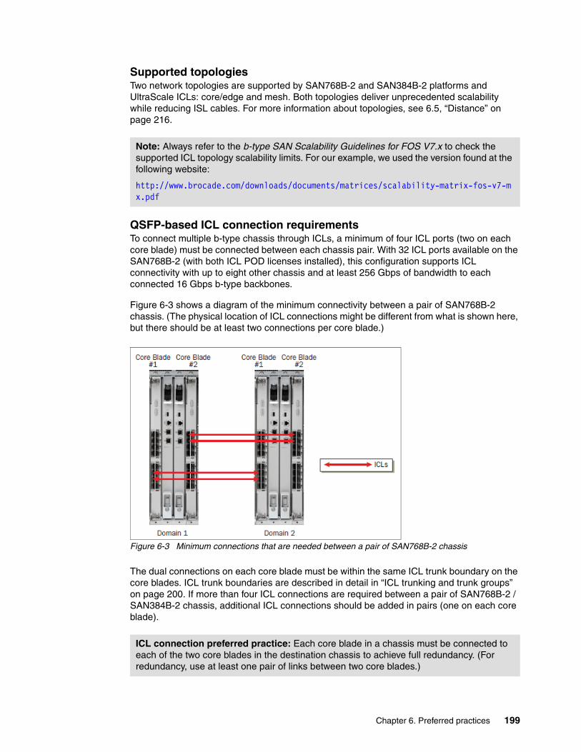
Supported topologiesTwo network topologies are supported by SAN768B-2 and SAN384B-2 platforms and UltraScale ICLs: core/edge and mesh. Both topologies deliver unprecedented scalability while reducing ISL cables. For more information about topologies, see 6.5, “Distance” on page 216.
QSFP-based ICL connection requirementsTo connect multiple b-type chassis through ICLs, a minimum of four ICL ports (two on each core blade) must be connected between each chassis pair. With 32 ICL ports available on the SAN768B-2 (with both ICL POD licenses installed), this configuration supports ICL connectivity with up to eight other chassis and at least 256 Gbps of bandwidth to each connected 16 Gbps b-type backbones.
Figure 6-3 shows a diagram of the minimum connectivity between a pair of SAN768B-2 chassis. (The physical location of ICL connections might be different from what is shown here, but there should be at least two connections per core blade.)
Figure 6-3 Minimum connections that are needed between a pair of SAN768B-2 chassis
The dual connections on each core blade must be within the same ICL trunk boundary on the core blades. ICL trunk boundaries are described in detail in “ICL trunking and trunk groups” on page 200. If more than four ICL connections are required between a pair of SAN768B-2 / SAN384B-2 chassis, additional ICL connections should be added in pairs (one on each core blade).
Note: Always refer to the b-type SAN Scalability Guidelines for FOS V7.x to check the supported ICL topology scalability limits. For our example, we used the version found at the following website:
http://www.brocade.com/downloads/documents/matrices/scalability-matrix-fos-v7-mx.pdf
ICL connection preferred practice: Each core blade in a chassis must be connected to each of the two core blades in the destination chassis to achieve full redundancy. (For redundancy, use at least one pair of links between two core blades.)
Chapter 6. Preferred practices 199

A maximum of 16 ICL connections or ICL trunk groups between any pair of SAN768B-2 / SAN384B-2 chassis is supported, unless they are deployed using Virtual Fabrics, where a maximum of 16 ICL connections or trunks can be assigned to a single Logical Switch. This limitation is because of the maximum supported number of connections for FSPF routing. Effectively, this means that there should never be more than 16 ICL connections or trunks between a pair of SAN768B-2 / SAN384B-2 chassis, unless Virtual Fabrics is enabled, and the ICLs are assigned to two or more Logical Switches. The exception to this is if eight port trunks are created between a pair of SAN768B-2 / SAN384B-2 chassis, as described in “ICL trunking and trunk groups”.
QSFP-based ICLs and traditional ISLs are not concurrently supported between a single pair of SAN768B-2 / SAN384B-2 chassis. All inter-chassis connectivity between any pair of SAN768B-2 / SAN384B-2 chassis must be done by using either ISLs or ICLs. The final layout and design of ICL interconnectivity is determined by the customer’s unique requirements and needs, which dictate the ideal number and placement of ICL connections between SAN768B-2 / SAN384B-2 chassis.
ICL trunking and trunk groupsTrunking involves taking multiple physical connections between a chassis or switch pair and forming a single “virtual” connection, aggregating the bandwidth for traffic to traverse across. This section describes the trunking capability that is used with the QSFP-based ICL ports on the IBM b-type 16 Gbps chassis platforms. (Trunking is enabled automatically for ICL ports, and it cannot be disabled by the user.)
Each QSFP-based ICL port has four independent 16 Gbps links, each of which terminates on one of four ASICs on each SAN768B-2 core blade, or two ASICs on each SAN384B-2 core blade. Trunk groups can be formed by using any of the ports that make up contiguous groups of eight links on each ASIC.
Figure 6-4 on page 201 shows that each core blade has groups of eight ICL ports (indicated by the blue box around the groups of ports) that connect to common ASICs in such a way that their four links can participate in common trunk groups with links from the other ports in the group.
200 IBM b-type Gen 5 16 Gbps Switches and Network Advisor

Figure 6-4 Core blade trunk groups
Each SAN384B-2 core blade has one group of eight ICL ports, and each SAN768B-2 core blade has two groups of eight ICL ports.
Because there are four separate links for each QSFP-based ICL connection, each of these ICL port groups can create up to four trunks, with up to eight links in each trunk.
A trunk can never be formed by links within the same QSFP ICL port because each of the four links within the ICL port terminates on a different ASIC for the SAN768B-2 core blade, or on either different ASICs or different trunk groups within the same ASIC for the SAN384B-2 core blade. Thus, each of the four links from an individual ICL is always part of independent trunk groups.
When connecting ICLs between a SAN768B-2 and a SAN384B-2, the maximum number of links in a single trunk group is four because the different number of ASICs on each product’s core blades, and the mapping of the ICL links to the ASIC trunk groups. To form trunks with up to eight links, ICL ports must be deployed within the trunk group boundaries that are shown in Figure 6-4, and they can be created only when deploying ICLs between a pair of SAN768B-2 chassis or SAN384B-2 chassis. It is not possible to create trunks with more than four links when connecting ICLs between a SAN768B-2 and SAN384B-2 chassis.
Chapter 6. Preferred practices 201

As a preferred practice, deploy trunk groups in groups of up to four links by ensuring that the ICL ports intended to form trunks all are within the groups that are indicated by the red boxes in Figure 6-5.
Figure 6-5 Core blade recommended trunk groups
If you follow this preferred practice, trunks can be easily formed by using ICL ports, whether you are connecting two SAN768B-2 chassis, two SAN384B-2 chassis, or a SAN768B-2 and a SAN384B-2.
Any time additional ICL connections are added to a chassis, they should be added in pairs by including at least one additional ICL on each core blade. It is also a preferred practice that trunks on a core blade are always composed of equal numbers of links, and that you deploy connections in an identical fashion on both core blades within a chassis. As an example, if you deploy two ICLs within the group of four ICL ports in trunk group A in Figure 6-5, you can add a single additional ICL to trunk group A, or you can add a pair of ICLs to any of the other trunk groups on the core blade. This ensures that no trunks are formed that have a different total bandwidth from other trunks on the same blade. Deploying a single additional ICL to trunk group B might result in four trunks with 32 Gbps of capacity (those created from the ICLs in trunk group A) and four trunks with only 16 Gbps (those from the single ICL in group B).
The port mapping information that is shown in Figure 6-6 on page 203 and Figure 6-7 on page 203 also indicates the recommended ICL trunk groups by showing ports in the same recommended trunk group with the same color.
Core blade (CR16-8) port numbering layoutFigure 6-6 on page 203 shows the layout of ports 0 - 15 on the SAN768B-2 CR16-8 line card. You can also see what the switchshow output would be if you ran a switchshow command within FOS by using the CLI.
202 IBM b-type Gen 5 16 Gbps Switches and Network Advisor
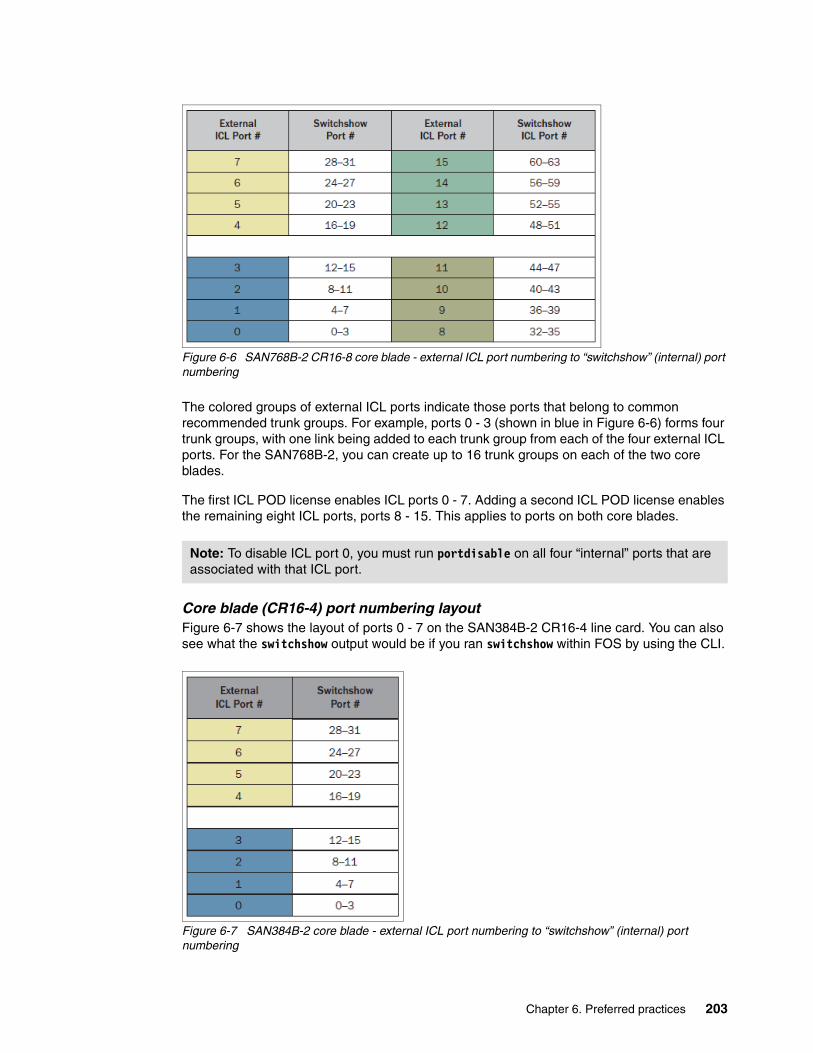
Figure 6-6 SAN768B-2 CR16-8 core blade - external ICL port numbering to “switchshow” (internal) port numbering
The colored groups of external ICL ports indicate those ports that belong to common recommended trunk groups. For example, ports 0 - 3 (shown in blue in Figure 6-6) forms four trunk groups, with one link being added to each trunk group from each of the four external ICL ports. For the SAN768B-2, you can create up to 16 trunk groups on each of the two core blades.
The first ICL POD license enables ICL ports 0 - 7. Adding a second ICL POD license enables the remaining eight ICL ports, ports 8 - 15. This applies to ports on both core blades.
Core blade (CR16-4) port numbering layoutFigure 6-7 shows the layout of ports 0 - 7 on the SAN384B-2 CR16-4 line card. You can also see what the switchshow output would be if you ran switchshow within FOS by using the CLI.
Figure 6-7 SAN384B-2 core blade - external ICL port numbering to “switchshow” (internal) port numbering
Note: To disable ICL port 0, you must run portdisable on all four “internal” ports that are associated with that ICL port.
Chapter 6. Preferred practices 203
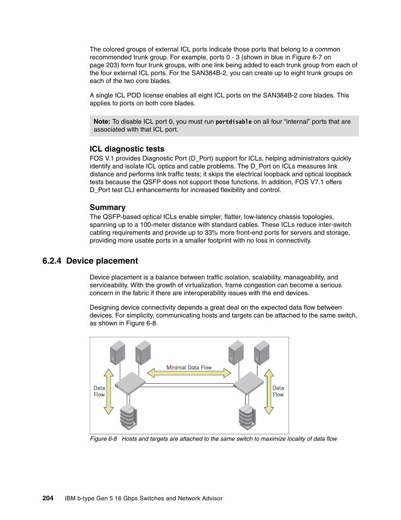
The colored groups of external ICL ports indicate those ports that belong to a common recommended trunk group. For example, ports 0 - 3 (shown in blue in Figure 6-7 on page 203) form four trunk groups, with one link being added to each trunk group from each of the four external ICL ports. For the SAN384B-2, you can create up to eight trunk groups on each of the two core blades.
A single ICL POD license enables all eight ICL ports on the SAN384B-2 core blades. This applies to ports on both core blades.
ICL diagnostic testsFOS V.1 provides Diagnostic Port (D_Port) support for ICLs, helping administrators quickly identify and isolate ICL optics and cable problems. The D_Port on ICLs measures link distance and performs link traffic tests; it skips the electrical loopback and optical loopback tests because the QSFP does not support those functions. In addition, FOS V7.1 offers D_Port test CLI enhancements for increased flexibility and control.
SummaryThe QSFP-based optical ICLs enable simpler, flatter, low-latency chassis topologies, spanning up to a 100-meter distance with standard cables. These ICLs reduce inter-switch cabling requirements and provide up to 33% more front-end ports for servers and storage, providing more usable ports in a smaller footprint with no loss in connectivity.
6.2.4 Device placement
Device placement is a balance between traffic isolation, scalability, manageability, and serviceability. With the growth of virtualization, frame congestion can become a serious concern in the fabric if there are interoperability issues with the end devices.
Designing device connectivity depends a great deal on the expected data flow between devices. For simplicity, communicating hosts and targets can be attached to the same switch, as shown in Figure 6-8.
Figure 6-8 Hosts and targets are attached to the same switch to maximize locality of data flow
Note: To disable ICL port 0, you must run portdisable on all four “internal” ports that are associated with that ICL port.
204 IBM b-type Gen 5 16 Gbps Switches and Network Advisor

However, this approach does not scale well. With the high-speed, low-latency nature of Fibre Channel, attaching these host-target pairs on different switches does not mean that performance is adversely impacted. Although traffic congestion is possible (see Figure 6-9), it can be mitigated with proper provisioning of ISLs/ICLs. With current generation switches, locality is not required for performance or to reduce latencies. For mission-critical applications, architects might want to localize the traffic when using solid-state devices (SSDs) or in exceptional cases, particularly if the number of ISLs available is restricted or there is a concern for resiliency in a multi-hop environment.
Figure 6-9 Hosts and targets are attached to different switches for ease of management and expansion
One common scheme for scaling a core-edge topology is dividing the edge switches in to a storage tier and a host/initiator tier. This approach lends itself to ease of management and expansion. In addition, host and storage devices generally have different performance requirements, cost structures, and other factors that can be readily accommodated by placing initiators and targets in different tiers.
The topology that is shown in Figure 6-10 provides a clearer distinction between the functional tiers.
Figure 6-10 Device type based edge-core-edge tiered topology
Here are some preferred practices for device placement:
� The preferred practice fabric topology is core-edge or edge-core-edge with tiered device connectivity, or full-mesh if the port count is less than 1500 ports.
� Minimize the use of localized traffic patterns and, if possible, keep servers and storage connected to separate switches.
� Select the appropriate optics (SWL/LWL/ELWL) to support the distance between switches and devices and switches.
Chapter 6. Preferred practices 205
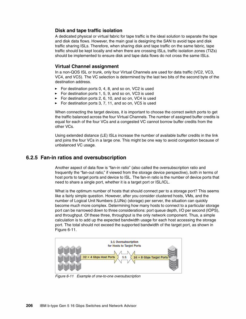
Disk and tape traffic isolationA dedicated physical or virtual fabric for tape traffic is the ideal solution to separate the tape and disk data flows. However, the main goal is designing the SAN to avoid tape and disk traffic sharing ISLs. Therefore, when sharing disk and tape traffic on the same fabric, tape traffic should be kept locally and when there are crossing ISLs, traffic isolation zones (TIZs) should be implemented to ensure disk and tape data flows do not cross the same ISLs.
Virtual Channel assignmentIn a non-QOS ISL or trunk, only four Virtual Channels are used for data traffic (VC2, VC3, VC4, and VC5). The VC selection is determined by the last two bits of the second byte of the destination address.
� For destination ports 0, 4, 8, and so on, VC2 is used� For destination ports 1, 5, 9, and so on, VC3 is used� For destination ports 2, 6, 10, and so on, VC4 is used� For destination ports 3, 7, 11, and so on, VC5 is used
When connecting the target devices, it is important to choose the correct switch ports to get the traffic balanced across the four Virtual Channels. The number of assigned buffer credits is equal for each of the four VCs and a congested VC cannot borrow buffer credits from the other VCs.
Using extended distance (LE) ISLs increase the number of available buffer credits in the link and joins the four VCs in a large one. This might be one way to avoid congestion because of unbalanced VC usage.
6.2.5 Fan-in ratios and oversubscription
Another aspect of data flow is “fan-in ratio” (also called the oversubscription ratio and frequently the “fan-out ratio,” if viewed from the storage device perspective), both in terms of host ports to target ports and device to ISL. The fan-in ratio is the number of device ports that need to share a single port, whether it is a target port or ISL/ICL.
What is the optimum number of hosts that should connect per to a storage port? This seems like a fairly simple question. However, after you consider clustered hosts, VMs, and the number of Logical Unit Numbers (LUNs) (storage) per server, the situation can quickly become much more complex. Determining how many hosts to connect to a particular storage port can be narrowed down to three considerations: port queue depth, I/O per second (IOPS), and throughput. Of these three, throughput is the only network component. Thus, a simple calculation is to add up the expected bandwidth usage for each host accessing the storage port. The total should not exceed the supported bandwidth of the target port, as shown in Figure 6-11.
Figure 6-11 Example of one-to-one oversubscription
206 IBM b-type Gen 5 16 Gbps Switches and Network Advisor

In practice, it is highly unlikely that all hosts perform at their maximum level at any one time. With the traditional application-per-server deployment, the Host Bus Adapter (HBA) bandwidth is over-provisioned. However, with virtual servers (KVM, Xen, Hyper-V, proprietary UNIX OSs, and VMware), the situation can change radically. Network oversubscription is built in to the virtual server concept. To the extent that servers use virtualization technologies, you should reduce network-based oversubscription proportionally. It might be prudent to oversubscribe ports to ensure a balance between cost and performance. An example of three-to-one oversubscription is shown in Figure 6-12.
Figure 6-12 Example of three-to-one oversubscription
Typical and safe oversubscription between the host and the edge is about 12:1. This is a good starting point for many deployments, but might need to be tuned based on the requirements. If you are in a highly virtualized environment with higher speeds and feeds, you might need to go lower than 12:1.
Preferred practices for avoiding frame congestion (when the number of frames is the issue rather than bandwidth usage) include:
� Use more and smaller trunks.
� Bandwidth through the core (path from source/host to destination/target) should exceed storage requirements.
� Host-to-core subscription ratios should be based on both the application needs and the importance of the application.
� Plan for peaks, not average usage.
� For mission-critical applications, the ratio should exceed peak load enough such that path failures do not adversely impact the application. Have enough extra bandwidth to avoid congestion if a link fails.
6.2.6 FCoE as a ToR solution
The consolidation of server network adapters, cables, and intermediate switches provides much of the motivation for implementing FCoE. The reduction in equipment, power, and maintenance costs is anticipated to be significant over time. With 10GbE widely used, FCoE technology might be a good choice for new environments with a high density of servers. It requires a Data Center Bridging (DCB) network to take advantage of new features such as Ethernet and Priority-based flow control (PFC), enhanced transmission selection (ETS), and Data Center Bridging Exchange (DCBX) Protocol.
Note: When the performance expectations are demanding, then we recommend a three-to-one oversubscription ratio, although 7:1 and even 16:1 are common.
Chapter 6. Preferred practices 207

In a FCoE edge topology, the ToR switch handles all the LAN and SAN traffic within a rack and forwards traffic to separate existing LAN and SAN infrastructures elsewhere in the data center. In general, vendors might allow their Fibre Channel Forwarders to operate in fabric mode or in NPIV mode. NPIV simplifies the implementation and avoids some incompatibility and management issues. For an IBM BladeCenter® chassis, IBM provides a set of switch modules and converged network adapters that easily allow the convergence of the LAN and SAN traffic.
Innovation and market trend also play an important role when you decide to choose FCoE for new SANs.
For more information, see Storage and Network Convergence Using FCoE and iSCSI, SG24-7986, found at:
http://www.redbooks.ibm.com/redbooks/pdfs/sg247986.pdf
6.2.7 NPIV and the access gateway
One of the main limits to Fibre Channel scalability is the maximum number of domains (individual physical or virtual switches) in a fabric. Keeping the number of domains low reduces much of the impact that is typically attributed to SAN fabrics. Small-domain-count fabrics are more reliable, perform better, and are easier to manage. When configuring the edge switches in Access Gateway (NPV for Cisco or Transparent for Qlogic) mode, the mode eliminates the usage of a domain ID.
In an environment with multivendor edge switches, the NPIV feature allows those switches to be presented in a transparent mode to the fabric, which reduces interoperability issues.
Regarding security issues, BladeCenter switches belong to the chassis and can be accessed through the management module. Sometimes, there is some confusion or conflict because the servers and SAN are usually managed by different teams. Configuring the BladeCenter switches in NPIV mode simplifies the topology and reduces the risk to the overall SAN fabric. All the Fibre Channel services are available to them by proxy.
NPIV can also be used by a hypervisor allowing a physical HBA to register with a Fabric using multiple (virtual) WWPNs. Each virtual WWPN can be assigned to a VM. These hypervisors can also be connected to an Access Gateway.
6.3 Data flow considerations
An important consideration when designing your SAN is understanding the data flow across the devices, as it might cause unwanted problems. This section describes some situations regarding data flow and what you can do to mitigate them.
6.3.1 Congestion in the fabric
Congestion is a major source of poor performance in a fabric. Sufficiently impeded traffic translates directly into poor application performance.
There are two major types of congestion: traffic-based and frame-based. Traffic-based congestion occurs when link throughput capacity is reached or exceeded and the link is no longer able to pass more frames. Frame-based congestion occurs when a link has run out of buffer credits and is waiting for buffers to free up to continue transmitting frames.
208 IBM b-type Gen 5 16 Gbps Switches and Network Advisor

6.3.2 Traffic-based versus frame-based congestion
After link speeds reach 4 Gbps and beyond, the emphasis on fabric and application performance shifts from traffic-level issues to frame congestion. It is difficult with current link speeds and features such as ISL Trunking or ICLs to consistently saturate a link. Most infrastructures today rarely see even two-member trunks reaching a sustained 100% usage. Frame congestion can occur when the buffers that are available on a Fibre Channel port are not sufficient to support the number of frames that the connected devices want to transmit. This situation can result in credit starvation backing up across the fabric. This condition is called back pressure, and it can cause severe performance problems.
One side effect of frame congestion can be large buffer credit zero counts on ISLs and F_Ports. This is not necessarily a concern, unless counts increase rapidly in a short period. There is a new feature, Bottleneck Detection, to more accurately assess the impact of a lack of buffer credits.
The sources and mitigation for traffic are known and are described at length in other parts of this book. The remainder of this section focuses on the sources and mitigation of frame-based congestion.
6.3.3 Sources of congestion
Frame congestion is primarily caused by latencies somewhere in the SAN, usually storage devices and occasionally hosts. These latencies cause frames to be held in ASICs and reduce the number of buffer credits that are available to all flows traversing that ASIC. The congestion backs up from the source of the latency to the other side of the connection and starts clogging up the fabric. This situation creates what is called back pressure. Back pressure can be created from the original source of the latency to the other side and all the way back (through other possible paths across the fabric, to the original source again. After this situation arises, the fabric is vulnerable to severe performance problems.
Sources of high latencies include the following items:
� Storage devices that are not optimized or where performance deteriorated over time
� Distance links where the number of allocated buffers is miscalculated or where the average frame sizes of the flows traversing the links changed over time
� Hosts where the application performance deteriorated to the point that the host can no longer respond to incoming frames in a sufficiently timely manner
Other contributors to frame congestion include behaviors where short frames are generated in large numbers:
� Clustering software that verifies the integrity of attached storage
� Clustering software that uses control techniques such as SCSI RESERVE/RELEASE to serialize access to shared file systems
� Host-based mirroring software that routinely sends SCSI control frames for mirror integrity checks
� Virtualizing environments, both workload and storage, that use in-band Fibre Channel for other control purposes
Chapter 6. Preferred practices 209

6.3.4 Mitigating congestion with Edge Hold Time
Frame congestion cannot be corrected in the fabric. Devices exhibiting high latencies, whether servers or storage arrays, must be examined and the source of poor performance eliminated. Because these are the major sources of frame congestion, eliminating them typically addresses the vast majority of cases of frame congestion in fabrics.
Introduction to Edge Hold TimeEdge Hold Time (EHT) is a FOS capability that allows an overriding value for Hold Time (HT). Hold Time is the amount of time a Class 3 frame may remain in a queue before being dropped while waiting for credit to be given for transmission.
The default HT is calculated from the RA_TOV, ED_TOV, and maximum hop count values that are configured on a switch. When you use the standard 10 seconds for RA_TOV, 2 seconds for ED_TOV, and a maximum hop count of 7, a Hold Time value of 500 ms is calculated. Extensive field experience has shown that when high latencies occur even on a single initiator or device in a fabric that not only does the F-port that is attached to this device see Class 3 frame discards, but the resulting back pressure because of the lack of credit can build up in the fabric and cause other flows that are not directly related to the high latency device to have their frames discarded at ISLs.
Edge Hold Time can be used to reduce the likelihood of this back pressure into the fabric by assigning a lower Hold Time value only for edge ports (initiators or devices). The lower EHT value ensures that frames are dropped at the F-port where the credit is lacking before the higher default Hold Time value that used at the ISLs expires, allowing these frames to begin moving again. This action localizes the impact of a high latency F-Port to just the single edge where the F-Port is and prevents the back pressure from spreading into the fabric and impacting other unrelated flows.
Like Hold Time, Edge Hold Time is configured for the entire switch, and is not configurable on individual ports or ASICs. Whether the EHT or HT values are used on a port depends on the particular platform and ASIC and the type of port and also other ports that are on the same ASIC. This behavior is described in further detail in the following sections.
Supported releases and licensing requirementsEHT was introduced in FOS V6.3.1b and is supported in FOS V6.3.2x, V6.4.0x, V6.4.1x, V6.4.2x, V6.4.3x, and all V7.X releases. Some behaviors have changed in later releases and are noted in later sections. There is no license that is required to configure the Edge Hold Time setting. Edge Hold Time must be explicitly enabled in all supporting FOS V6.x releases. In FOS V7.0 and later, EHT is enabled by default.
BehaviorThis section describes the behavior on the different platforms.
8 Gb platforms and the 2109-M48On the IBM 2109-M48 and all 8 Gb platforms, including the 2499-384/2499-192, Hold Time is an ASIC level setting that is applied to all ports on the same ASIC chip. If any single port on the ASIC chip is an F-Port, then the alternative EHT value is programmed into the ASIC, and all ports (E-Ports and F-Ports) use this one value. If all ports on the single ASIC chip are E-Ports, then the entire ASIC is programmed with the default Hold Time value (500 ms).
210 IBM b-type Gen 5 16 Gbps Switches and Network Advisor

When Virtual Fabrics are enabled on an 8 Gb switch, the programming of the ASIC remains at the ASIC level. If any single port on the ASIC is an F-Port, regardless of which Logical Switch it is in, then the alternative EHT value is programmed in to the ASIC for all ports in all Logical Switches, regardless of the port type.
For example, if one ASIC has five ports that are assigned to Logical Switch 1, which has four F-Ports and one E-Port, and this same ASIC has five ports that are assigned to Logical Switch 2, which has all E-Ports, the EHT value is programmed into all five ports in Logical Switch 1 and also all five ports in Logical Switch 2. The programming of EHT is at the ASIC level and is applied across Logical Switch boundaries.
When you use Virtual Fabrics, the EHT value that is configured into the Base Switch is the value that is used for all Logical Switches.
Gen 5 platformsAll b-type Gen 5 platforms (16 Gb) can set the Hold Time value on a port-by-port basis for ports that are on Gen 5 ASICs. All F-ports are programmed with the alternative Edge Hold Time. All E-Ports are programmed with the default Hold Time value (500 ms). The same EHT value set for the switch is programmed into all F-Ports on that switch. Different EHT values cannot be programmed on an individual port basis.
If 8 Gb blades are installed into a Gen 5 platform (that is, an FC8-64 blade in an IBM 2499-816/2499-416 chassis), then the behavior of EHT on the 8 Gb blades is the same as the description that is provided for 8 Gb platforms. The same EHT value is programmed in to all ports on the ASIC.
If any single port on an ASIC is an F-Port, then the alternative EHT value is programmed in to the ASIC, and all ports (E-Ports and F-Ports) use this one value.
If all ports on an ASIC are E-Ports, then the entire ASIC is programmed with the default Hold Time value (500 ms).
When you deploy Virtual Fabrics with FOS Versions 7.0.0x, 7.0.1x, or 7.0.2x, the EHT value that is configured into the Default Switch is the value that is used for all Logical Switches.
Starting with FOS V7.1.0, a unique EHT value can be independently configured for each Logical Switch for Gen 5 Platforms. 8 Gb blades that are installed in a Gen 5 platform continue to use the Default Logical Switch configured value for all ports on those blades regardless of which Logical Switches those ports are assigned to.
Default EHT settingsThe default setting that is used for Edge Hold Time (EHT) is preinstalled into the switch at the factory based on the version of FOS that is installed. The settings are shown in Table 6-2.
Table 6-2 Factory default EHT settings
Factory installed version of FOS Default EHT value
Any version of FOS V7.X 220 ms
FOS V6.4.3x 500 ms
FOS V6.4.2x 500 ms
FOS V6.4.1x 220 ms
FOS V6.4.0x 500 ms
Any version before FOS V6.4.0 500 ms
Chapter 6. Preferred practices 211

You can change the default setting by running configure command. You can change the EHT without having to disable the switch; the change takes effect immediately.
When you run configure to set EHT, a suggested EHT value is provided. If you accept this suggested setting by pressing Enter, then this suggested value becomes the new value for EHT on the switch.
The suggested value is the value that was set during the previous time the configure command was run, even if the user just pressed the Enter key when encountering this configuration parameter. If the configure command has never been run before, and thus the default value is what is set in the system, then the suggested value that is shown is what is shown in Table 6-3.
Table 6-3 Suggested EHT settings for various FOS releases
The suggested value that is shown when you run the configure command might not be the same as the default value that is running in the system. This is because the default EHT value is set based on the FOS version that was installed at the factory, and the suggested EHT value is based on the FOS version currently running in the system and whether the configure command had ever been run in the past.
After it is set by the configure command, the EHT value is maintained across firmware upgrades, power cycles, and HA failover operations. This is true for all versions of FOS. The behavior of EHT evolved over several FOS releases. The three different behaviors are shown in the three different examples that follow.
Example 6-1 shows an FOS V6.x configure command.
Example 6-1 FOS V6.x
sw0:FID128:admin> configureNot all options will be available on an enabled switch.To disable the switch, use the “switchDisable” command.Configure...Fabric parameters (yes, y, no, n): [no] yConfigure edge hold time (yes, y, no, n): [no] yEdge hold time: (100..500) [500]System services (yes, y, no, n): [no]
Example 6-2 shows an FOS V7.0.x configure command.
Example 6-2 FOS V7.0.x
sw0:FID128:admin> configureNot all options will be available on an enabled switch.
FOS version currently on switch Suggested EHT value when configure has not been run previously
Any version of FOS V7.X 220 ms
FOS V6.4.3x 500 ms
FOS V6.4.2x 500 ms
FOS V6.4.1x 220 ms
FOS V6.4.0x 500 ms
Any version before FOS V6.4.0 500 ms
212 IBM b-type Gen 5 16 Gbps Switches and Network Advisor

To disable the switch, use the “switchDisable” command.Configure...Fabric parameters (yes, y, no, n): [no] yEdge Hold Time (0 = Low(80ms),1 = Medium(220ms),2 = High(500ms): [220ms]: (0..2) [1]System services (yes, y, no, n): [no]
Example 6-3 shows an FOS V7.0.2 and higher configure command.
Example 6-3 FOS V7.0.2 and higher
sw0:FID128:admin> configureNot all options will be available on an enabled switch.To disable the switch, use the “switchDisable” command.Configure...Fabric parameters (yes, y, no, n): [no] yEdge Hold Time in ms (80(Low), 220(Medium), 500(High), 80-500(UserDefined)): (80..500) [220]System services (yes, y, no, n): [no]
Recommended settingsEdge Hold Time does not need to be set on “core switches” that are composed of only ISLs and therefore use only the standard Hold Time setting of 500 ms. Recommended values for platforms containing initiators and targets are based on specific deployment strategies. Users typically either separate initiators and targets on separate switches or mix initiators and targets on the same switch.
A frame drop has more significance for a target than an initiator because many initiators typically communicate with a single target port, whereas target ports typically communicate with multiple initiators. Frame drops on target ports usually result in “SCSI Transport” error messages being generated in server logs. Multiple frame drops from the same target port can affect multiple servers in what appears to be a random fabric or storage problem. Because the source of the error is not obvious, this can result in time that is wasted determining the source of the problem. Extra care should be taken therefore when you apply EHT to switches where targets are deployed.
The most common recommended value for EHT is 220 ms. The lowest EHT value of 80 ms should be configured only on edge switches comprised entirely of initiators. This lowest value is recommended for fabrics that are maintained and when a more aggressive monitoring and protection strategy is being deployed.
6.4 Redundancy and resiliency
An important aspect of SAN topology is the resiliency and redundancy of the fabric. The main objective is to remove any single point of failure. Resiliency is the ability of the network to continue to function or recover from a failure, while redundancy describes duplication of components, even an entire fabric, to eliminate a single point of failure in the network. The FOS code provides resiliency that is built in the software that can quickly “repair” the network to overcome most failures. For example, when a link between switches fails, routing is quickly recalculated and traffic is assigned to the new route. This assumes that there is a second route, which is when redundancy in the fabric becomes important.
Chapter 6. Preferred practices 213
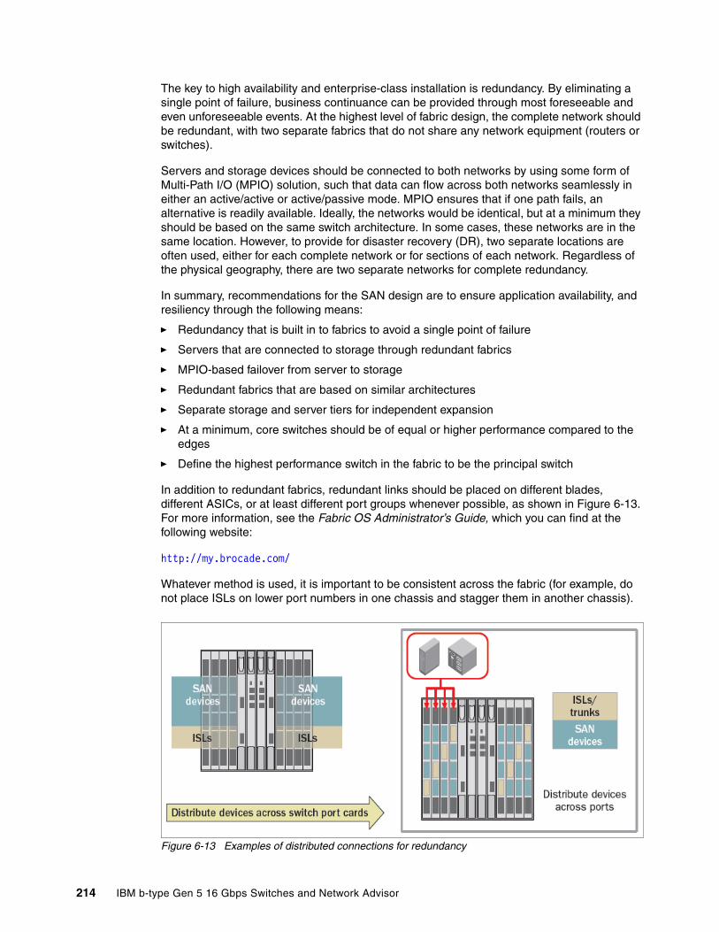
The key to high availability and enterprise-class installation is redundancy. By eliminating a single point of failure, business continuance can be provided through most foreseeable and even unforeseeable events. At the highest level of fabric design, the complete network should be redundant, with two separate fabrics that do not share any network equipment (routers or switches).
Servers and storage devices should be connected to both networks by using some form of Multi-Path I/O (MPIO) solution, such that data can flow across both networks seamlessly in either an active/active or active/passive mode. MPIO ensures that if one path fails, an alternative is readily available. Ideally, the networks would be identical, but at a minimum they should be based on the same switch architecture. In some cases, these networks are in the same location. However, to provide for disaster recovery (DR), two separate locations are often used, either for each complete network or for sections of each network. Regardless of the physical geography, there are two separate networks for complete redundancy.
In summary, recommendations for the SAN design are to ensure application availability, and resiliency through the following means:
� Redundancy that is built in to fabrics to avoid a single point of failure
� Servers that are connected to storage through redundant fabrics
� MPIO-based failover from server to storage
� Redundant fabrics that are based on similar architectures
� Separate storage and server tiers for independent expansion
� At a minimum, core switches should be of equal or higher performance compared to the edges
� Define the highest performance switch in the fabric to be the principal switch
In addition to redundant fabrics, redundant links should be placed on different blades, different ASICs, or at least different port groups whenever possible, as shown in Figure 6-13. For more information, see the Fabric OS Administrator’s Guide, which you can find at the following website:
http://my.brocade.com/
Whatever method is used, it is important to be consistent across the fabric (for example, do not place ISLs on lower port numbers in one chassis and stagger them in another chassis).
Figure 6-13 Examples of distributed connections for redundancy
214 IBM b-type Gen 5 16 Gbps Switches and Network Advisor

For more information about fabric resiliency preferred practices, see Fabric Resiliency Best Practices, REDP-4722, found at:
http://www.redbooks.ibm.com/abstracts/redp4722.html?OpenHigh Availability
High availability can be built in to the fabric by eliminating single points of failure. This is achieved by deploying hardware components in redundant pairs, and configuring redundant paths. Redundant paths are routed through different switches to provide availability of connection. If there is a path failure (for example, because of an HBA, port card, fiber-optic cable, or storage adapter), software running on the host servers initiates failover to a secondary path. If the path failover malfunctions, the application fails. Then, the only choice is to repair the failed path, or replace the failed device. Both these actions potentially lead to outages of other applications on multiple heterogeneous servers if the device affected is the switch.
6.4.1 Single point of failure
By definition, a single point of failure (SPoF) is a part of a system/component that, if it fails, stops the entire system from working. These components can be HBAs, power supplies, ISLs, switches, or even entire fabrics. Fabrics are typically deployed in pairs, mirroring one another in topology and configuration, and (unless routing is being used) are isolated from one another. The assessment of a potential SPoF involves identifying the critical components of a complex system that might provoke a total systems failure in case of malfunction.
Note: In Figure 6-13 on page 214, ISLs and SAN devices are placed on separate ASICs or port groups. Also, the EHT feature is ASIC-dependent, and the setting applies to all the ports on the ASIC. In environments with high-latency devices, place devices and ISLs on separate ASICs when possible.
Chapter 6. Preferred practices 215
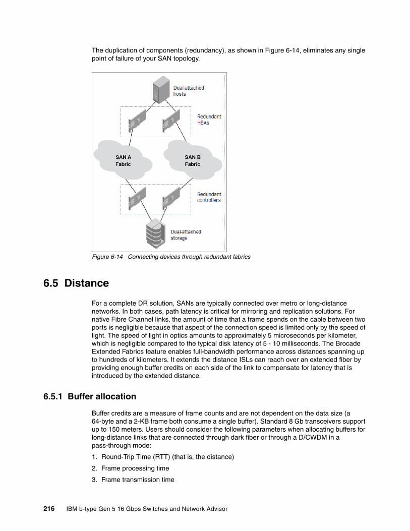
The duplication of components (redundancy), as shown in Figure 6-14, eliminates any single point of failure of your SAN topology.
Figure 6-14 Connecting devices through redundant fabrics
6.5 Distance
For a complete DR solution, SANs are typically connected over metro or long-distance networks. In both cases, path latency is critical for mirroring and replication solutions. For native Fibre Channel links, the amount of time that a frame spends on the cable between two ports is negligible because that aspect of the connection speed is limited only by the speed of light. The speed of light in optics amounts to approximately 5 microseconds per kilometer, which is negligible compared to the typical disk latency of 5 - 10 milliseconds. The Brocade Extended Fabrics feature enables full-bandwidth performance across distances spanning up to hundreds of kilometers. It extends the distance ISLs can reach over an extended fiber by providing enough buffer credits on each side of the link to compensate for latency that is introduced by the extended distance.
6.5.1 Buffer allocation
Buffer credits are a measure of frame counts and are not dependent on the data size (a 64-byte and a 2-KB frame both consume a single buffer). Standard 8 Gb transceivers support up to 150 meters. Users should consider the following parameters when allocating buffers for long-distance links that are connected through dark fiber or through a D/CWDM in a pass-through mode:
1. Round-Trip Time (RTT) (that is, the distance)
2. Frame processing time
3. Frame transmission time
216 IBM b-type Gen 5 16 Gbps Switches and Network Advisor

Here are some good general guidelines:
� Number of credits = 6 + ((link speed Gbps * Distance in KM) / frame size in KB).
Example: 100 KM @2k frame size = 6 + ((8 Gbps * 100) / 2) = 406
� A buffer model should be based on the average frame size.
� If compression is used, the number of buffer credits that is needed is 2x the number of credits without compression.
On the IBM b-type 16 Gbps backbones platform, 4 K buffers are available per ASIC to drive the 16 Gbps line rate to 500 KM at a 2 KB frame size. FOS V7.1 provides users with additional control when they configure a port of an LD or LS link, which allows users to specify the buffers that are required or the average frame size for a long-distance port. Using the frame size option, the number of buffer credits that are required for a port is automatically calculated. These options give users additional flexibility to optimize performance on long-distance links.
In addition, FOS V7.1 provides users better insight into long-distance link traffic patterns by displaying the average buffer usage and average frame size through the CLI. FOS V7.1 also provides a new CLI portBufferCalc command that automatically calculates the number of buffers that are required per port given the distance, speed, and frame size. The number of buffers that is calculated by this command can be used when you configure the portCfgLongDistance command. If no options are specified, then the current port’s configuration is used to calculate the number of buffers that are required.
6.5.2 Fabric interconnectivity over Fibre Channel at longer distances
SANs spanning data centers in different physical locations can be connected through dark fiber connections by using Extended Fabrics, which is a FOS optionally licensed feature, with wave division multiplexing, such as Dense Wave Division Multiplexing (DWDM), Coarse Wave Division Multiplexing (CWDM), and Time Division Multiplexing (TDM). This situation is similar to connecting switches in the data center with one exception: Additional buffers are allocated to E_Ports connecting over distance. The Extended Fabrics feature extends the distance the ISLs can reach over an extended fiber. This task is accomplished by providing enough buffer credits on each side of the link to compensate for the latency that is introduced by the extended distance. Use the buffer credit calculation or the new CLI tools with FOS V7.1 to determine the number of buffers that is needed to support the required performance.
Any of the first eight 8 ports on the 16 Gbps port blade can be set to 10 Gbps FC for connecting to a 10 Gbps line card D/CWDM without needing a specialty line card. If you connect to DWDMs in a pass-through mode where the switch is providing all the buffering, a 16 Gbps line rate can be used for higher performance.
Here are some preferred practices:
� Connect the cores of each fabric to the DWDM.
� If you use trunks, use smaller and more trunks on separate port blades for redundancy and to provide more paths. Determine the optimal number of trunk groups between each set of linked switches, depending on traffic patterns and port availability.
Note: The D_Port mode can also be used to measure the cable distance to a granularity of 5 meters between two 16 Gbps platforms; however, ports must be offline.
Chapter 6. Preferred practices 217

6.5.3 Fibre Channel over IP
Fibre Channel over IP (FCIP) links are most commonly used for Remote Data Replication (RDR) and remote tape applications for the purpose of Business Continuance/Disaster Recovery. Transporting data over significant distances beyond the reach of a threatening event preserves the data so that an organization can recover from that event. A device that transports FCIP is often called a channel extender.
RDR is typically storage array to array communications. The local array at the production site sends data to the other array at the backup site. This task can be done through native FC if the backup site is within a practical distance and there is DWDM or dark fiber between the sites. However, more commonly what is available is a cost-sensitive infrastructure for IP connectivity and not native FC connectivity. The current technology for FCIP is high speed and adds only a minute amount (about 35 µs) of propagation delay, which is appropriate for asynchronous RDR and tape applications and synchronous RDR applications.
The preferred practice for the deployment of FCIP channel extenders in RDR applications is to connect the FC F_Ports on the channel extender directly to the FC N_Ports on the array, and not go through the production fabric at all. On most large-scale arrays, the FC port that is assigned to RDR is dedicated to only RDR and no host traffic. Considering that the RDR port on the array can communicate only RDR traffic, there is no need to run that port into the production fabric. There are valid reasons to go through a production fabric, such as IBM SAN Volume Controller, which has requirements for connectivity to the production fabric.
Figure 6-15 shows an example of how to incorporate the production fabrics into the FCIP path.
Figure 6-15 Four device solution that is connected to production fabrics
Even though the example shows an additional component (SAN06B-R) that fulfills the role of an FCIP path, you can use the SAN768B-2 or SAN384B-2 with the 8 Gbps Extension Blade (FC3890) to fulfill the same FCIP function.
In environments that require production fabric attached channel extenders, it is not a preferred practice to connect the same channel extender to both “A” and “B” fabrics. The preferred practice is to have two redundant FC fabrics in all production environments in which an organization would suffer losses if the SAN were to go down. Even a momentary outage can “blue screen” or hang servers, which requires them to be rebooted, which can take a significant amount of time in some situations. The division of the “A” and “B” fabrics implies that there is an air gap between the two autonomous fabrics from the server to the storage array. There are no physical data links between the two independent fabrics. The servers are equipped with FC software drivers (in our example, ESXi native Multi-Path I/O) for their HBAs that monitor the individual paths sending data across all of them.
218 IBM b-type Gen 5 16 Gbps Switches and Network Advisor
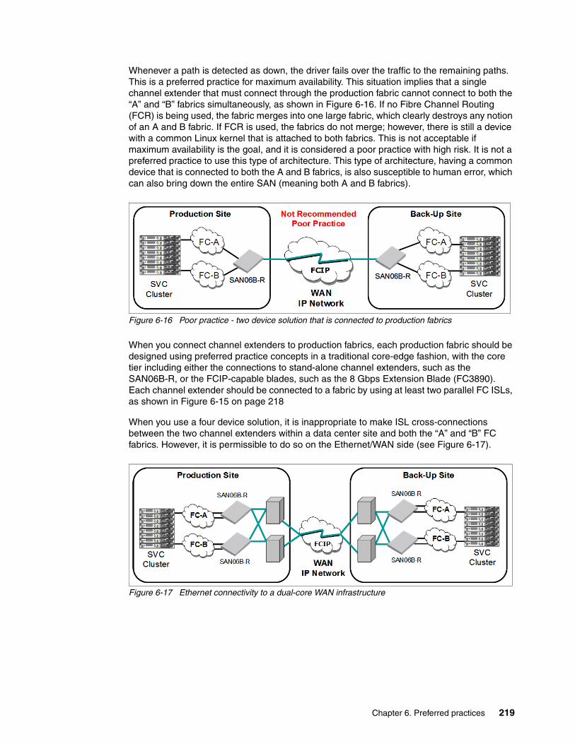
Whenever a path is detected as down, the driver fails over the traffic to the remaining paths. This is a preferred practice for maximum availability. This situation implies that a single channel extender that must connect through the production fabric cannot connect to both the “A” and “B” fabrics simultaneously, as shown in Figure 6-16. If no Fibre Channel Routing (FCR) is being used, the fabric merges into one large fabric, which clearly destroys any notion of an A and B fabric. If FCR is used, the fabrics do not merge; however, there is still a device with a common Linux kernel that is attached to both fabrics. This is not acceptable if maximum availability is the goal, and it is considered a poor practice with high risk. It is not a preferred practice to use this type of architecture. This type of architecture, having a common device that is connected to both the A and B fabrics, is also susceptible to human error, which can also bring down the entire SAN (meaning both A and B fabrics).
Figure 6-16 Poor practice - two device solution that is connected to production fabrics
When you connect channel extenders to production fabrics, each production fabric should be designed using preferred practice concepts in a traditional core-edge fashion, with the core tier including either the connections to stand-alone channel extenders, such as the SAN06B-R, or the FCIP-capable blades, such as the 8 Gbps Extension Blade (FC3890). Each channel extender should be connected to a fabric by using at least two parallel FC ISLs, as shown in Figure 6-15 on page 218
When you use a four device solution, it is inappropriate to make ISL cross-connections between the two channel extenders within a data center site and both the “A” and “B” FC fabrics. However, it is permissible to do so on the Ethernet/WAN side (see Figure 6-17).
Figure 6-17 Ethernet connectivity to a dual-core WAN infrastructure
Chapter 6. Preferred practices 219

6.5.4 FCIP with FCR
The FCIP tunnel traditionally traverses a WAN or IP cloud, which can have characteristics that adversely impact a Fibre Channel network. The FCIP link across a WAN is essentially an FC ISL over an IP link. In any design, it should be considered an FC ISL. Repeated flapping of a WAN connection can cause disruption in directly connected fabrics. This disruption might come about from the many fabric services trying to reconverge again and again. This situation causes the processor on the switch or director to go to full capacity. If the processor can no longer process the various tasks that are required to operate a fabric, there might be an outage. If you limit the fabric services to within the local fabric itself and do not allow them to span across the WAN, you can prevent this situation from occurring. FCR provides a termination point for fabric services, referred to as a demarcation point. EX_Ports and VEX_Ports are demarcation points in which fabric services are terminated, forming the “edge” to the fabric. A fabric that is isolated in such a way is referred to as an “edge fabric.” There is a special case in which the edge fabric includes the WAN link because a VEX_Port was used; this type of edge fabric is referred to as a remote edge fabric.
FCR does not need to be used unless there is a production fabric that must be isolated from WAN outages. When connecting to array ports directly for RDR, FCR provides no benefit. Mainframe environments are precluded from using FCR, as it is not supported by FICON.
When a mainframe host writes to a volume on the direct access storage device (DASD), and that DASD performs RDR to another DASD, then DASD to DASD traffic is not using FICON. It is using an open systems RDR application such as IBM Metro Mirror or Global Mirror. These open-system RDR applications can use FCR, even though the volumes they are replicating are written by the FICON host.
Here are some basic FCR architectures:
� No FCR or one large fabric: This type of architecture is used with the mainframe and when the channel extenders are directly connected to the storage arrays.
� Edge-backbone-edge: Edge fabrics bookend a transit backbone between them.
� VEX_Port: When a VEX_Port is used, the resulting architecture can be either backbone-remote edge or edge-backbone-remote edge, depending on whether devices are connected directly to the backbone or an edge fabric hangs from the backbone. Both are possible.
6.5.5 Using EX_Ports and VEX_Ports
If an FCR architecture is indicated, an “X” port is needed. An “X” port is a generic reference for an EX_Port or a VEX_Port. The only difference between an EX_Port and a VEX_Port is that the “V” indicates that it is FCIP-facing. The same holds true for E_Ports and VE_Ports; VE_Ports are E_Ports that are FCIP-facing.
The preferred practice in an FC routed environment is to build an edge fabric to backbone to edge fabric (EBE) topology. This topology provides isolation of fabric services in both edge fabrics. This topology requires an EX_Port from the backbone to connect to an E_Port in the edge fabric, as shown in Figure 6-18 on page 221. The backbone fabric continues to be exposed to faults in the WAN connections, but because its scope is limited by the VE_Ports in each edge fabric, and because edge fabric services are not exposed to the backbone, it does not pose any risk of disruption to the edge fabrics in terms of overrunning the processors or causing a fabric service to become unavailable. The edge fabric services do not span the backbone.
220 IBM b-type Gen 5 16 Gbps Switches and Network Advisor
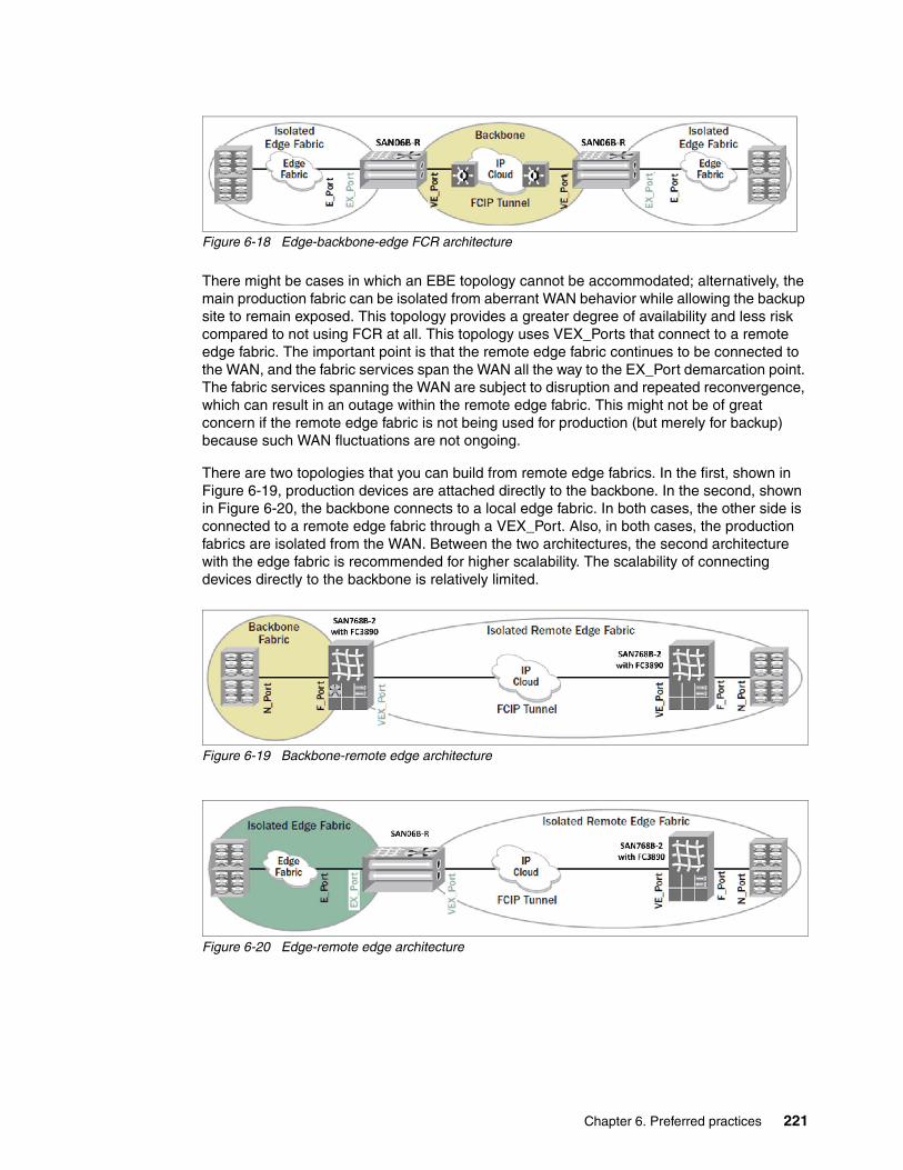
Figure 6-18 Edge-backbone-edge FCR architecture
There might be cases in which an EBE topology cannot be accommodated; alternatively, the main production fabric can be isolated from aberrant WAN behavior while allowing the backup site to remain exposed. This topology provides a greater degree of availability and less risk compared to not using FCR at all. This topology uses VEX_Ports that connect to a remote edge fabric. The important point is that the remote edge fabric continues to be connected to the WAN, and the fabric services span the WAN all the way to the EX_Port demarcation point. The fabric services spanning the WAN are subject to disruption and repeated reconvergence, which can result in an outage within the remote edge fabric. This might not be of great concern if the remote edge fabric is not being used for production (but merely for backup) because such WAN fluctuations are not ongoing.
There are two topologies that you can build from remote edge fabrics. In the first, shown in Figure 6-19, production devices are attached directly to the backbone. In the second, shown in Figure 6-20, the backbone connects to a local edge fabric. In both cases, the other side is connected to a remote edge fabric through a VEX_Port. Also, in both cases, the production fabrics are isolated from the WAN. Between the two architectures, the second architecture with the edge fabric is recommended for higher scalability. The scalability of connecting devices directly to the backbone is relatively limited.
Figure 6-19 Backbone-remote edge architecture
Figure 6-20 Edge-remote edge architecture
Chapter 6. Preferred practices 221
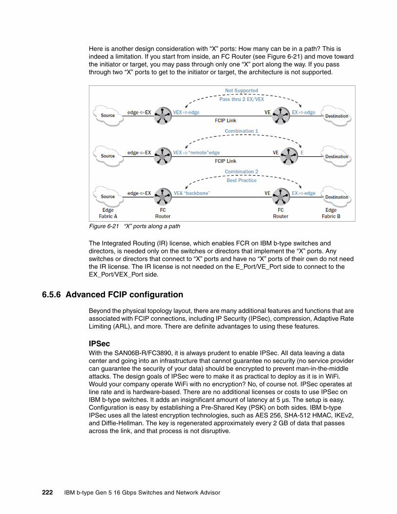
Here is another design consideration with “X” ports: How many can be in a path? This is indeed a limitation. If you start from inside, an FC Router (see Figure 6-21) and move toward the initiator or target, you may pass through only one “X” port along the way. If you pass through two “X” ports to get to the initiator or target, the architecture is not supported.
Figure 6-21 “X” ports along a path
The Integrated Routing (IR) license, which enables FCR on IBM b-type switches and directors, is needed only on the switches or directors that implement the “X” ports. Any switches or directors that connect to “X” ports and have no “X” ports of their own do not need the IR license. The IR license is not needed on the E_Port/VE_Port side to connect to the EX_Port/VEX_Port side.
6.5.6 Advanced FCIP configuration
Beyond the physical topology layout, there are many additional features and functions that are associated with FCIP connections, including IP Security (IPSec), compression, Adaptive Rate Limiting (ARL), and more. There are definite advantages to using these features.
IPSecWith the SAN06B-R/FC3890, it is always prudent to enable IPSec. All data leaving a data center and going into an infrastructure that cannot guarantee no security (no service provider can guarantee the security of your data) should be encrypted to prevent man-in-the-middle attacks. The design goals of IPSec were to make it as practical to deploy as it is in WiFi. Would your company operate WiFi with no encryption? No, of course not. IPSec operates at line rate and is hardware-based. There are no additional licenses or costs to use IPSec on IBM b-type switches. It adds an insignificant amount of latency at 5 µs. The setup is easy. Configuration is easy by establishing a Pre-Shared Key (PSK) on both sides. IBM b-type IPSec uses all the latest encryption technologies, such as AES 256, SHA-512 HMAC, IKEv2, and Diffie-Hellman. The key is regenerated approximately every 2 GB of data that passes across the link, and that process is not disruptive.
222 IBM b-type Gen 5 16 Gbps Switches and Network Advisor
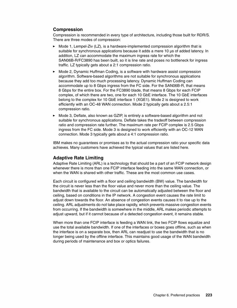
CompressionCompression is recommended in every type of architecture, including those built for RDR/S. There are three modes of compression:
� Mode 1, Lempel-Ziv (LZ), is a hardware-implemented compression algorithm that is suitable for synchronous applications because it adds a mere 10 µs of added latency. In addition, LZ can accommodate the maximum ingress rate for which the SAN06B-R/FC3890 has been built, so it is line rate and poses no bottleneck for ingress traffic. LZ typically gets about a 2:1 compression ratio.
� Mode 2, Dynamic Huffman Coding, is a software with hardware assist compression algorithm. Software-based algorithms are not suitable for synchronous applications because they add too much processing latency. Dynamic Huffman Coding can accommodate up to 8 Gbps ingress from the FC side. For the SAN06B-R, that means 8 Gbps for the entire box. For the FC3890 blade, that means 8 Gbps for each FCIP complex, of which there are two, one for each 10 GbE interface. The 10 GbE interfaces belong to the complex for 10 GbE interface 1 (XGE1). Mode 2 is designed to work efficiently with an OC-48 WAN connection. Mode 2 typically gets about a 2.5:1 compression ratio.
� Mode 3, Deflate, also known as GZIP, is entirely a software-based algorithm and not suitable for synchronous applications. Deflate takes the tradeoff between compression ratio and compression rate further. The maximum rate per FCIP complex is 2.5 Gbps ingress from the FC side. Mode 3 is designed to work efficiently with an OC-12 WAN connection. Mode 3 typically gets about a 4:1 compression ratio.
IBM makes no guarantees or promises as to the actual compression ratio your specific data achieves. Many customers have achieved the typical values that are listed here.
Adaptive Rate LimitingAdaptive Rate Limiting (ARL) is a technology that should be a part of an FCIP network design whenever there is more than one FCIP interface feeding into the same WAN connection, or when the WAN is shared with other traffic. These are the most common use cases.
Each circuit is configured with a floor and ceiling bandwidth (BW) value. The bandwidth for the circuit is never less than the floor value and never more than the ceiling value. The bandwidth that is available to the circuit can be automatically adjusted between the floor and ceiling, based on conditions in the IP network. A congestion event causes the rate limit to adjust down towards the floor. An absence of congestion events causes it to rise up to the ceiling. ARL adjustments do not take place rapidly, which prevents massive congestion events from occurring. If the bandwidth is somewhere in the middle, ARL makes periodic attempts to adjust upward, but if it cannot because of a detected congestion event, it remains stable.
When more than one FCIP interface is feeding a WAN link, the two FCIP flows equalize and use the total available bandwidth. If one of the interfaces or boxes goes offline, such as when the interface is on a separate box, then ARL can readjust to use the bandwidth that is no longer being used by the offline interface. This maintains good usage of the WAN bandwidth during periods of maintenance and box or optics failures.
Chapter 6. Preferred practices 223

In Figure 6-22, the black circuit is feeding the WAN, after which the red circuit comes online. The black and red circuits find equilibrium, as their aggregate bandwidth is equal to the available WAN bandwidth. When the red circuit goes offline again, the bandwidth is freed and the black circuit intermittently tests for that bandwidth and increases the rate limiting to take advantage of it. This continues until the ceiling is reached again.
Figure 6-22 Adaptive Rate Limiting behavior for two flows
In a shared link situation, if you think of the bandwidth as separated into three areas, black (0 x bps), gray (x y bps), and white (y maximum bps), ARL can help manage the bandwidth usage. Black is the floor value for ARL. This is the amount of bandwidth that is reserved exclusively for FCIP. White is the ceiling value, and it is reserved exclusively for other shared traffic. Gray is the area in between, which FCIP may use if other shared traffic is not using it. This other shared traffic can also be another FCIP application, such as tape. Black would be the RDR traffic; white would be tape traffic, and they adaptively share the gray area. There are many ways in which you can use ARL; these are just a few examples.
PerPriority TCP QoSDifferentiated Services Code Point (DSCP) is an IP-based (L3) quality of service (QoS) marking; because IP is end-to-end protocol, DSCP is an end-to-end QoS marking. DSCP has 64 values; however, the range of values 0 - 63 do not denote the lowest priority through the highest priority. The valuing system works differently. First, all odd numbers are available for private use and can be used in any way that enterprise deems valuable. These odd numbers are for private use the same way that RFC 1918 IP addresses are; for example, 192.168.0.1 and 10.1.2.3 are private IP addresses that can be used in any way an enterprise wants.
224 IBM b-type Gen 5 16 Gbps Switches and Network Advisor

For non-private DSCP values, DSCP value 46 is referred to as Expedited Forwarding and is the highest priority. Zero is the default, and it is the lowest priority. There are four groups of High/Medium/Low (H/M/L) values referred to as Assured Forwarding. Another group of numbers has compatibility with legacy Type of Service (ToS). The selection of DSCP to be used in the IP network is the responsibility of the IP network administrators. Without their buy-in and configuration of the Per-Hop Behavior (PHB) that is associated with QoS, no QoS can happen. The default behavior of Ethernet switches is to replace ingress QoS values with the default value (0), unless the data coming in on that interface is explicitly deemed to be QoS “trusted.” This situation prevents users from setting their own QoS values unannounced to the IP networking administrators.
802.1P is data link-based (L2) QoS marking; therefore, the scope extends only from the interface of one device to the interface of the directly attached device. Devices that enforce 802.1P provide QoS across that data link. 802.1P has a header that is in the 802.1Q VLAN tagging header; therefore, VLAN tagging is required to get 802.1P QoS marking. Brocade FOS refers to 802.1P as L2CoS. There are only eight values for 802.1P, that is, 0 - 7. Zero is the lowest priority and the default. Seven is the highest priority.
The SAN06B-R/FC3890 supports three levels of priority (H/M/L). The default amount of BW that the scheduler apportions during times of contention is 50/30/20%. QoS portioning of BW occurs only during times of contention; otherwise, the BW is shared equally across all priorities. It is possible to change the default portions to any values you want, if High>Middle>Low and the aggregate of all the priorities equals 100%.
There are four TCP sessions per FCIP circuit: H, M, L, and F-Class. F-Class uses a strict queuing, which means that if there is any F-Class traffic to send, it all gets sent first. There is little F-Class traffic, and it does not interfere with data traffic. Each TCP session is autonomous and does not rely on other TCP sessions or settings. Each TCP session can be configured with its own DSCP, VLAN tagging, and 802.1P values. This permits that TCP session (priority) to be treated independently in the IP network from site-to-site based on the SLA for that QoS priority.
Brocade has QoS in Brocade FC/FICON fabrics and across FC ISLs through Virtual Channels (VCs). There are different VCs for H/M/L/F-Class, each with its own set of Buffer-to-Buffer Credits and flow control. There are five VCs for high levels, four VCs for medium levels, and two VCs for low levels. Devices are assigned to QoS VCs by enabling QoS on the fabric and then putting the letters QOSH_ or QOSL_ as a prefix to the zone name. The default is QOSM_, so there is no need to explicitly designate medium zones. After devices are assigned to these VCs, they use these VCs throughout the fabric. If data ingresses to a SAN06B-R/FC3890 through an ISL on a particular VC, the data is automatically assigned to the associated TCP sessions for that priority. Devices that are directly connected to the SAN06B-R/FC3890 are also assigned to the associated TCP session priority based on the zone name prefix.
DSCP and L2CoS are configured on a per-FCIP circuit basis. Do not alter the QoS markings for F-Class traffic unless it is required to differentiate and expedite F-Class traffic across the IP network between the sites. Failure of F-class traffic to arrive in a timely manner causes instability in the FC fabric. This is less of an issue with directly connected separate RDR networks. FCIP networks that must o be connected to the production FC fabrics can use FCR (IR license) to protect the edge fabrics from instability.
Chapter 6. Preferred practices 225

6.5.7 FCIP design preferred practices
For RDR, the preferred practice is to use a separate and dedicated IP connection between the production data center and the backup site. Often, a dedicated IP connection between data centers is not practical. In this case, bandwidth must at least be logically dedicated. There are a few ways this can be done:
� Use QoS, and give FCIP a high priority. This logically dedicates enough bandwidth to FCIP over other traffic.
� Use Committed Access Rate (CAR) to identify and rate-limit certain traffic types. Use CAR on the non-FCIP traffic to apportion and limit that traffic to a maximum amount of bandwidth, leaving the remainder of the bandwidth to FCIP. Set the aggregate FCIP rate limit on the SAN06B-R switch or FC3890 blade to use the remaining portion of the bandwidth. This results in logically dedicating bandwidth to FCIP.
� It is possible, with massive overprovisioning of bandwidth, for various traffic types to coexist over the same IP link. Brocade FCIP uses an aggressive TCP stack that is called Storage Optimized TCP (SO-TCP), which dominates other TCP flows within the IP link, causing them to back off dramatically. If the other flows are UDP-based, the result is considerable congestion and excessive dropped packets for all traffic.
A preferred practice is to always rate limit the FCIP traffic on the SAN06B-R or FC3890 blade and never rate limit FCIP traffic in the IP network, which often leads to problems that are difficult to troubleshoot. The rate limiting technology on the SAN06B-R/FC3890 is advanced, accurate, and consistent, so there is no need to double rate limit. If a policy requires you to double the rate limit, then the IP network should set its rate limiting above that of the SAN06B-R/FC3890 with plenty of headroom.
To determine the amount of network bandwidth that is needed, gather a month’s worth of data by using various tools that are host-, fabric-, and storage-based. It is important to understand the host–to-disk traffic because that is the amount of traffic to be replicated, or mirrored, to the remote disk.
If you are going to be doing synchronous RDR (RDR/S), then record peak values. If you are going to be using asynchronous RDR (RDR/A), then record the average value over the hour. RDR/S must have enough bandwidth to send the write I/O immediately; therefore, there must be enough bandwidth to accommodate the entire demand, which is peak value. RDR/A needs only enough bandwidth to accommodate the high average that is discovered over an adequate recording period because RDR/A essentially performs traffic shaping, moving the peaks into the troughs, which works out to the average. It cannot be the average over a long period because those troughs might not occur soon enough to relieve the array of the peaks. This causes excessive journaling of data, which is difficult to recover from.
Plot the values into a histogram. More than likely, you get a Gaussian curve (see Figure 6-23 on page 227). Most of the averages fall within the first standard deviation of the curve, which is 68.2% of the obtained values. The second standard deviation includes 95.4% of the obtained values, which are enough samples to determine the bandwidth you need. Outside of this, the values are corner cases, which most likely can be accommodated by the FCIP network because of their infrequency. Use a bandwidth utilization value that you are comfortable with between and 2. You can plan for a certain amount of compression, such as 2:1. However, a preferred practice is to use compression as a way to address future bandwidth needs. It is probably best not to push the limit right at the start because then you have nowhere to go in the near future.
226 IBM b-type Gen 5 16 Gbps Switches and Network Advisor

Figure 6-23 Gaussian curve
You can take advantage of FCIP Trunking to implement redundant network routes from site to site. But it is important to understand whether traffic can fail over to the alternative route transparently or whether that impacts traffic flow.
For disk extension using emulation (FastWrite), a single tunnel between sites is recommended. If multiple tunnels must be used, use Traffic Isolation (TI) zones or logical switch configuration to ensure that the same exchange always traverses by the same tunnel in both directions. Use multiple circuits instead of multiple tunnels for redundancy and failover protection.
6.5.8 FCIP Trunking
The SAN06B-R and FC3890 have an exclusive feature called FCIP Trunking. FCIP Trunking offers the ability to perform the following functions:
� Bandwidth aggregation� Lossless failover/failback� Granular load balancing� In-order delivery� Prevention of IFCC on mainframes
A single tunnel that is defined by a VE_Port or VEX_Port might have one or more circuits that are associated with it. A circuit is an FCIP connection that is defined by a source and destination IP address and other arguments that define its characteristics, such as compression, IPSec, QoS, rate limit, and VLAN tag. All the circuits terminate at the single VE/VEX_Port on each side; therefore, there are no multiple tunnels or ISLs, but only a single tunnel load balanced across multiple circuits. The one ISL that an FCIP Trunk forms is from VE_Port to VE_Port or VEX_Port to VE_Port.
The circuits can have different characteristics. They can have different RTTs and take different paths and different service providers. They can have different bandwidths up to 4x. This means that if one circuit is an OC-3, the most the other circuits can be is OC-12 because the bandwidth delta is 4x.
Chapter 6. Preferred practices 227
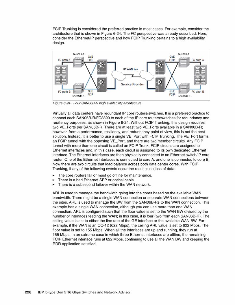
FCIP Trunking is considered the preferred practice in most cases. For example, consider the architecture that is shown in Figure 6-24. The FC perspective was already described. Here, consider the Ethernet/IP perspective and how FCIP Trunking pertains to a high availability design.
Figure 6-24 Four SAN06B-R high availability architecture
Virtually all data centers have redundant IP core routers/switches. It is a preferred practice to connect each SAN06B-R/FC3890 to each of the IP core routers/switches for redundancy and resiliency purposes, as shown in Figure 6-24. Without FCIP Trunking, this design requires two VE_Ports per SAN06B-R. There are at least two VE_Ports available in a SAN06B-R; however, from a performance, resiliency, and redundancy point of view, this is not the best solution. Instead, it is better to use a single VE_Port with FCIP Trunking. The VE_Port forms an FCIP tunnel with the opposing VE_Port, and there are two member circuits. Any FCIP tunnel with more than one circuit is called an FCIP Trunk. FCIP circuits are assigned to Ethernet interfaces and, in this case, each circuit is assigned to its own dedicated Ethernet interface. The Ethernet interfaces are then physically connected to an Ethernet switch/IP core router. One of the Ethernet interfaces is connected to core A, and one is connected to core B. Now there are two circuits that load balance across both data center cores. With FCIP Trunking, if any of the following events occur the result is no loss of data:
� The core routers fail or must go offline for maintenance.� There is a bad Ethernet SFP or optical cable.� There is a subsecond failover within the WAN network.
ARL is used to manage the bandwidth going into the cores based on the available WAN bandwidth. There might be a single WAN connection or separate WAN connections between the sites. ARL is used to manage the BW from the SAN06B-Rs to the WAN connection. This example has a single WAN connection, although you can use more than one WAN connection. ARL is configured such that the floor value is set to the WAN BW divided by the number of interfaces feeding the WAN; in this case, it is four (two from each SAN06B-R). The ceiling value is set to either the line rate of the GE interface or the available WAN BW. For example, if the WAN is an OC-12 (622 Mbps), the ceiling ARL value is set to 622 Mbps. The floor value is set to 155 Mbps. When all the interfaces are up and running, they run at 155 Mbps. In an extreme case in which three Ethernet interfaces are offline, the remaining FCIP Ethernet interface runs at 622 Mbps, continuing to use all the WAN BW and keeping the RDR application satisfied.
228 IBM b-type Gen 5 16 Gbps Switches and Network Advisor
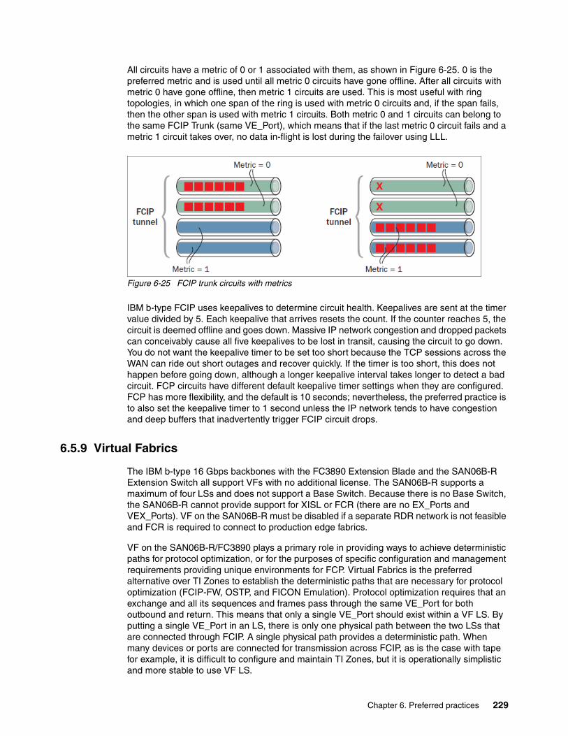
All circuits have a metric of 0 or 1 associated with them, as shown in Figure 6-25. 0 is the preferred metric and is used until all metric 0 circuits have gone offline. After all circuits with metric 0 have gone offline, then metric 1 circuits are used. This is most useful with ring topologies, in which one span of the ring is used with metric 0 circuits and, if the span fails, then the other span is used with metric 1 circuits. Both metric 0 and 1 circuits can belong to the same FCIP Trunk (same VE_Port), which means that if the last metric 0 circuit fails and a metric 1 circuit takes over, no data in-flight is lost during the failover using LLL.
Figure 6-25 FCIP trunk circuits with metrics
IBM b-type FCIP uses keepalives to determine circuit health. Keepalives are sent at the timer value divided by 5. Each keepalive that arrives resets the count. If the counter reaches 5, the circuit is deemed offline and goes down. Massive IP network congestion and dropped packets can conceivably cause all five keepalives to be lost in transit, causing the circuit to go down. You do not want the keepalive timer to be set too short because the TCP sessions across the WAN can ride out short outages and recover quickly. If the timer is too short, this does not happen before going down, although a longer keepalive interval takes longer to detect a bad circuit. FCP circuits have different default keepalive timer settings when they are configured. FCP has more flexibility, and the default is 10 seconds; nevertheless, the preferred practice is to also set the keepalive timer to 1 second unless the IP network tends to have congestion and deep buffers that inadvertently trigger FCIP circuit drops.
6.5.9 Virtual Fabrics
The IBM b-type 16 Gbps backbones with the FC3890 Extension Blade and the SAN06B-R Extension Switch all support VFs with no additional license. The SAN06B-R supports a maximum of four LSs and does not support a Base Switch. Because there is no Base Switch, the SAN06B-R cannot provide support for XISL or FCR (there are no EX_Ports and VEX_Ports). VF on the SAN06B-R must be disabled if a separate RDR network is not feasible and FCR is required to connect to production edge fabrics.
VF on the SAN06B-R/FC3890 plays a primary role in providing ways to achieve deterministic paths for protocol optimization, or for the purposes of specific configuration and management requirements providing unique environments for FCP. Virtual Fabrics is the preferred alternative over TI Zones to establish the deterministic paths that are necessary for protocol optimization (FCIP-FW, OSTP, and FICON Emulation). Protocol optimization requires that an exchange and all its sequences and frames pass through the same VE_Port for both outbound and return. This means that only a single VE_Port should exist within a VF LS. By putting a single VE_Port in an LS, there is only one physical path between the two LSs that are connected through FCIP. A single physical path provides a deterministic path. When many devices or ports are connected for transmission across FCIP, as is the case with tape for example, it is difficult to configure and maintain TI Zones, but it is operationally simplistic and more stable to use VF LS.
Chapter 6. Preferred practices 229
Configuring more than one VE_Port, one manually set with a higher FSPF cost, is referred to as a “lay in wait” VE_Port and it is not supported for FCIP-FW, OSTP, or FICON Emulation. A “lay in wait” VE_Port can be used without protocol optimization and with RDR applications that can tolerate the topology change and some frame loss. A few FC frames might be lost when you use “lay in wait” VE_Ports. If there are multiple VE_Ports within an LS, routing across those VE_Ports is performed according to the APTpolicy.
Virtual Fabrics are significant in mixed mainframe and open system environments. Mainframe and open system environments are configured differently and only VFs can provide autonomous LSs that accommodate the different configurations. Keep in mind that RDR between storage arrays is open systems (IBM Metro/Global Mirror), even when the volume is written by FICON from the mainframe.
Understand that using a VE_Port in a selected LS does not preclude that VE_Port from sharing an Ethernet interface with other VE_Ports in other LSs. This is referred to as Ethernet Interface Sharing.
6.5.10 Ethernet Interface Sharing
An FCIP Trunk uses multiple Ethernet interfaces by assigning the circuits that belong to that trunk to different Ethernet interfaces. IP interfaces (ipifs) are configured with IP addresses, subnet masks, and an Ethernet interface, which assigns the ipif to the interface. When the FCIP circuit is configured, the source IP address must be one that was used to configure an ipif, which in turn assigns the FCIP circuit to that Ethernet interface. It is possible to assign multiple IP addresses and circuits to the same Ethernet interface by assigning multiple ipif to that same interface, each with its own unique IP address.
Any one circuit cannot be shared across more than one Ethernet interface. An IP address/ipif/circuit can belong only to one Ethernet interface. Thus, if more than one Ethernet interface is wanted, you must use multiple circuits. If you attempt to configure the same IP address on more than one ipif, an error occurs and the configuration is rejected.
It is possible to share an Ethernet interface with multiple circuits that belong to different VF LSs. The Ethernet interface must be owned by the default switch (context 128). The ipif and IP route (iproute) must also be configured within the default switch. The VE_Port is assigned to the LS you want to extend with FCIP and is configured within that LS. The FCIP tunnel is also configured within that LS by using the IP addresses of the ipif that are in the default switch. This permits efficient usage of the 10 GbE interfaces.
Often, for purposes of redundancy and resiliency, an FCIP Trunk has circuits that extend out of both of the 10 GbE interfaces. Each 10 GbE interface (XGE) has “native” VE_Ports from one of the two groups (xge1:12-21 or xge0:22-31). If you want to extend a circuit from VE_Port 12 through xge0, you must use a cross-port. A cross-port requires an ipif and iproute that were configured and explicitly designated for cross-port use; otherwise, the circuit cannot be configured for the non-native 10 GbE interface. By merely designating the ipif and iproutes to be used with non-native XGE interfaces, you can configure this type of circuit.
230 IBM b-type Gen 5 16 Gbps Switches and Network Advisor
6.5.11 Workloads
Many different kinds of traffic traverse a SAN fabric. The mix of traffic is typically based on the workload on the servers and the effect that behavior has on the fabric and the connected storage. Here are examples of different types of workload:
� I/O-intensive, transaction-based applications: These systems typically do high volumes of short block I/O and do not consume much network bandwidth. These applications usually have high-performance service levels to ensure low response times. Care must be taken to ensure that there are a sufficient number of paths between the storage and hosts to ensure that other traffic does not interfere with the performance of the applications. These applications are also sensitive to latency.
� I/O-intensive applications: These applications perform long block or sequential I/O and generate much higher traffic levels than transaction-based applications (data mining). Depending on the type of storage, these applications can consume bandwidth and generate latency in both storage and hosts that can negatively impact the performance of other applications sharing their storage.
� Host High Availability (HA) clustering: These clusters often treat storage differently from stand-alone systems. They might, for example, continuously check their connected storage for data integrity reasons and put a strain on both the fabric and the storage arrays to which they are attached. This can result in frame congestion in the fabric and can cause performance problems in storage arrays.
� Host-based replication: Host-based replication causes traffic levels to increase significantly across a fabric and can put considerable pressure on ISLs. Replicating to poorer-performing storage (such as tier 1 to tier 2 storage) can cause application performance issues that are difficult to identify. Latencies in the slower storage can also cause “back pressure,” which can extend back into the fabric and slow down other applications that use the same ISLs.
� Array-based replication: Data can be replicated between storage arrays as well.
Workload virtualizationThere has been a huge growth in virtualized workloads in the past three years. Available on IBM mainframes for decades, workload virtualization initially was popularized on Intel-based platforms by VMware ESXi Host (now vSphere). Windows, UNIX, and Linux server virtualization is now ubiquitous in enterprise infrastructures.
Most recently, organizations started adopting workload virtualization for desktops. This technology is still in development but is evolving rapidly. (Desktop virtualization storage access is not addressed in this book.)
Chapter 6. Preferred practices 231
6.5.12 Intel -based virtualization storage access
Intel -based VMs typically access storage in two ways:
� They use some sort of distributed file system that is typically controlled by the hypervisor (the control program that manages VMs). This method puts the onus on the hypervisor to manage the integrity of VM data. All VM I/O passes through an I/O abstraction layer in the hypervisor, which adds extra processing to every I/O that a VM issues. The advantage to this approach is that many VMs can share a LUN (storage), making storage provisioning and management a relatively easy task. Today, most VMware deployments use this approach by deploying a file system called Shared VMFS.
� They create separate LUNs for each data store and allow VMs to access data directly through N_Port ID Virtualization (NPIV). The advantage of this approach is that VMs can access data more or less directly through a virtual HBA. The disadvantage is that there are many more LUNs to provision and manage.
Most VMs today tend to do little I/O (typically no more than a few MBps per VM through few IOPS). This allows many VMs to be placed on a single hypervisor platform without regard to the amount of I/O that they generate. Storage access is not a significant factor when converting a physical server to a virtual one. More important factors are memory usage and IP network usage.
The main storage-related issue when deploying virtualized PC applications is VM migration. If VMs share a LUN, and a VM is migrated from one hypervisor to another, the integrity of the LUN must be maintained. That means that both hypervisors must serialize access to the same LUN. Normally, this is done through mechanisms such as SCSI reservations. The more the VMs migrate, the potentially larger the serialization problem becomes. SCSI reservations can contribute to frame congestion and generally slow down VMs that are accessing the same LUN from several different hypervisor platforms.
Here are some design guidelines for virtualized storage:
� If possible, try to deploy VMs to minimize VM migrations if you are using shared LUNs.
� Use individual LUNs for any I/O-intensive applications such as SQL Server, Oracle databases, and Microsoft Exchange.
� Regarding monitoring, use Advanced Performance Monitoring and Fabric Watch to alert you to excessive levels of SCSI reservations. These notifications can save you much time by identifying VMs and hypervisors that are vying for access to the same LUN.
6.6 Security
There are many components to SAN security in relation to SAN design, and the decision to use these components depends on your installation requirements rather than network functioning or performance. One clear exception is the zoning feature that is used to control device communication. The proper use of zoning is key to fabric functioning, performance, and stability, especially in larger networks. Other security-related features are largely mechanisms for limiting access and preventing attacks on the network (and are mandated by regulatory requirements), and they are not required for normal fabric operation.
232 IBM b-type Gen 5 16 Gbps Switches and Network Advisor

6.6.1 Zone Management: Dynamic Fabric Provisioning (DFP)
The IBM b-type Fibre Channel (16 Gbps) SAN platforms with a Brocade HBA solution provide an integrated switch that enables customers to dynamically provision switch-generated virtual WWNs and create a fabric-wide zone database before acquiring and connecting any Brocade HBAs to the switch. DFP enables SAN administrators to pre-provision services such as zoning, QoS, Device Connection Control (DCC), or any services that require port-level authentication before servers that arrive in the fabric. This enables a more secure and flexible zoning scheme because the fabric assigns the WWN to use. The FA-WWN can be user-generated or fabric-assigned (FA-WWN). When an HBA is replaced or a server is upgraded, zoning and LUN mapping does not have to be changed because the new HBA is assigned the same FA-WWN as before. DFP is supported on both switches with or without the Access Gateway support. The switch automatically prevents assignment of duplicate WWNs by cross-referencing the name server database, but the SAN administrator has the ultimate responsibility to prevent duplicates from being created when WWNS are user-assigned.
6.6.2 Zone management: Duplicate WWNs
In a virtual environment such as VMware, it is possible to encounter duplicate WWNs in the fabric. This impacts the switch response to fabric services requests, such as “get port WWN”, resulting in unpredictable behavior. The fabric’s handling of duplicate WWNs is not meant to be an intrusion detection tool but a recovery mechanism. Before FOS V7.0, when a duplicate entry is detected, a warning message is sent to the RAS log, but no effort is made to prevent the login of the second entry.
Starting with FOS V7.0, here is how duplicate WWNs are handled:
� Same switch: The choice of which device stays in the fabric is configurable (default is to retain the existing device).
� Local and remote switches: Remove both entries.
Chapter 6. Preferred practices 233

Zoning recommendations include the following ones:
� Always enable zoning.
� Create zones with only one initiator (as shown in Figure 6-26) and ports from a single target device. Different target devices should not be zoned together. Specific zones should be created when different target devices need to communicate each other (that is, copy services).
� Define zones using device worldwide port names (WWPNs).
� The default zoning should be set to No Access.
� Use FA-WWN if it is supported by FOS (Version 7.0 or later) and Brocade HBA driver (Version 3.0 or later).
� Delete all Fabric-Assigned Port worldwide names (FA-PWWNs) from the switch whose configuration is being replaced before you upload or download a modified configuration.
� Follow vendor guidelines for preventing the generation of duplicate WWNs in a virtual environment.
� Use a consistent naming scheme for all components.
� If available, use automated tools to verify the proposed zoning changes.
� Remove any zoning items not in use.
Figure 6-26 Example of single initiator zones
6.6.3 Role-Based Access Controls
One way to provide limited accessibility to the fabric is through user roles. FOS has predefined user roles, each of which has access to a subset of the CLI commands. These roles are known as Role-Based Access Controls (RBACs), and they are associated with the user login credentials. When you log in to a switch, your user account is associated with a predefined role or a user-defined role. The role that your account is associated with determines the level of access you have on that switch and in the fabric. For more information about RBAC, see the Managing User Accounts chapter in the Fabric OS Administrator’s Guide, which you can find at the following website:
http://my.brocade.com/
234 IBM b-type Gen 5 16 Gbps Switches and Network Advisor
6.6.4 Default accounts
FOS offers four predefined accounts: admin, factory, root, and user. Although the root and factory accounts are reserved for development and manufacturing, the password for all default accounts should be changed and secured during the initial installation and configuration of each switch. Recovering passwords requires significant effort and fabric downtime.
6.6.5 Access control lists
Access control lists (ACLs) are used to provide network security through policy sets. FOS provides several ACL policies, including a Switch Connection Control (SCC) policy, a Device Connection Control (DCC) policy, a Fabric Configuration Server (FCS) policy, an IP Filter, and others. The following subsections briefly describe each policy and provide basic guidelines. A more in-depth description of ACLs can be found in the Fabric OS Administrator’s Guide, which you can find at the following website:
http://my.brocade.com/
SCC policyThe SCC policy restricts the fabric elements (FC switches) that can join the fabric. Only switches that are specified in the policy are allowed to join the fabric. All other switches fail authentication if they attempt to connect to the fabric, resulting in the respective E_Ports being segmented because of the security violation.
Use the SCC policy in environments where there is a need for strict control of fabric members. Because the SCC policy can prevent switches from participating in a fabric, it is important to regularly review and properly maintain the SCC ACL.
DCC policyThe DCC policy restricts the devices that can attach to a single FC port. The policy specifies the FC port and one or more WWNs that are allowed to connect to the port. The DCC policy set comprises all of the DCC policies that are defined for individual FC ports. (Not every FC port must have a DCC policy, and only ports with a DCC policy in the active policy set enforce access controls.) A port that is present in the active DCC policy set allows only WWNs in its respective DCC policy to connect and join the fabric. All other devices fail authentication when attempting to connect to the fabric, resulting in the respective F_Ports being disabled because of the security violation.
Use the DCC policy in environments where there is a need for strict control of fabric members. Because the DCC policy can prevent devices from participating in a fabric, it is important to regularly review and properly maintain the DCC policy set.
FCS policyUse the FCS policy to restrict the source of fabric-wide settings to one FC switch. The policy contains the WWN of one or more switches, and the first WWN (that is online) in the list is the primary FCS. If the FCS policy is active, then only the primary FCS is allowed to make or propagate fabric-wide parameters. These parameters include zoning, security (ACL) policies databases, and other settings.
Use the FCS policy in environments where there is a need for strict control of fabric settings. As with other ACL policies, it is important to regularly review and properly maintain the FCS policy.
Chapter 6. Preferred practices 235
IP FilterThe IP Filter policy is a set of rules that are applied to the IP management interfaces as a packet filtering firewall. The firewall permits or denies the traffic to go through the IP management interfaces according to the policy rules.
The IP Filter policy should be used in environments where there is a need for strict control of fabric access. As with other ACL policies, it is important to regularly review and properly maintain the IP Filter policy.
As a preferred practice, non-secure IP protocols that are used for switch management such as telnet and http should be blocked. SSH is enabled on the default IP Filter policy and SSL should be configured to use https for web access.
Authentication protocolsFOS supports both Fibre Channel Authentication Protocols (FCAPs) and Diffie-Hellman Challenge Handshake Authentication Protocols (DH-CHAPs) on E_Ports and F_Ports. Authentication protocols provide additional security during link initialization by ensuring that only the wanted device/device type is connecting to a given port.
6.6.6 Policy Database Distribution
Security Policy Database Distribution provides a mechanism for controlling the distribution of each policy on a per-switch basis. Switches can individually configure policies to either accept or reject a policy distribution from another switch in the fabric. In addition, a fabric-wide distribution policy can be defined for the SCC and DCC policies with support for strict, tolerant, and absent modes. This can be used to enforce whether the SCC or DCC policy must be consistent throughout the fabric.
The Policy Database Distribution has three modes:
� Strict mode: All updated and new policies of the type specified (SCC, DCC, or both) must be distributed to all switches in the fabric, and all switches must accept the policy distribution.
� Tolerant mode: All updated and new policies of the type specified (SCC, DCC, or both) are distributed to all switches (FOS V6.2.0 or later) in the fabric, but the policy does not need to be accepted.
� Absent mode: Updated and new policies of the type specified (SCC, DCC, or both) are not automatically distributed to other switches in the fabric; policies can still be manually distributed.
Together, the policy distribution and fabric-wide consistency settings provide a range of control on the security policies from little or no control to strict control.
6.6.7 In-flight encryption and compression: b-type (16 Gbps) platforms only
IBM b-type Fibre Channel (16 Gbps) platforms support both in-flight compression and encryption at a port level for both local and long-distance ISL links. In-flight data compression is a useful tool for saving money when either bandwidth caps or bandwidth usage charges are in place for transferring data between fabrics. Similarly, in-flight encryption enables a further layer of security with no key management impact when transferring data between local and long-distance data centers besides the initial setup.
236 IBM b-type Gen 5 16 Gbps Switches and Network Advisor
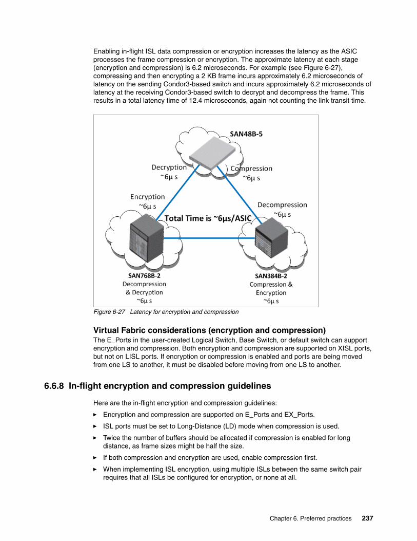
Enabling in-flight ISL data compression or encryption increases the latency as the ASIC processes the frame compression or encryption. The approximate latency at each stage (encryption and compression) is 6.2 microseconds. For example (see Figure 6-27), compressing and then encrypting a 2 KB frame incurs approximately 6.2 microseconds of latency on the sending Condor3-based switch and incurs approximately 6.2 microseconds of latency at the receiving Condor3-based switch to decrypt and decompress the frame. This results in a total latency time of 12.4 microseconds, again not counting the link transit time.
Figure 6-27 Latency for encryption and compression
Virtual Fabric considerations (encryption and compression)The E_Ports in the user-created Logical Switch, Base Switch, or default switch can support encryption and compression. Both encryption and compression are supported on XISL ports, but not on LISL ports. If encryption or compression is enabled and ports are being moved from one LS to another, it must be disabled before moving from one LS to another.
6.6.8 In-flight encryption and compression guidelines
Here are the in-flight encryption and compression guidelines:
� Encryption and compression are supported on E_Ports and EX_Ports.
� ISL ports must be set to Long-Distance (LD) mode when compression is used.
� Twice the number of buffers should be allocated if compression is enabled for long distance, as frame sizes might be half the size.
� If both compression and encryption are used, enable compression first.
� When implementing ISL encryption, using multiple ISLs between the same switch pair requires that all ISLs be configured for encryption, or none at all.
Chapter 6. Preferred practices 237
� No more than two ports on one ASIC can be configured with encryption, compression, or both when running at 16 Gbps speed. With FOS V7.1, additional ports can be used for data encryption, data compression, or both if running at lower than 16 Gbps speeds.
� Encryption is not compliant with Federal Information Processing Standards (FIPS).
6.7 Monitoring
Any mission-critical infrastructure must be properly monitored. Although there are many features that are available in FOS to assist you with monitoring, protecting, and troubleshooting fabrics, several recent enhancements were implemented that deal exclusively with this area. An overview of the major components is provided in the following sections. A complete guide to health monitoring is beyond the scope of this document. For more information, see the Fabric OS Command Reference Guide, the Fabric OS Troubleshooting Guide, and the appropriate SAN Health and Fabric Watch guides. You can find the the two FOS publications at the following website:
http://my.brocade.com/
6.7.1 Fabric Watch
Fabric Watch is an optional health monitor that allows you to constantly monitor each director or switch for potential faults and automatically alerts you to problems before they become costly failures.
Fabric Watch tracks various SAN fabric elements and events. Monitoring fabric-wide events, ports, and environmental parameters enables early fault detection and isolation and performance measurement. You can configure fabric elements and alert thresholds on an individual port basis, and you can also easily integrate Fabric Watch with enterprise system management solutions.
Fabric Watch provides customizable monitoring thresholds. You can configure Fabric Watch to provide notification before problems arise, such as reporting when network traffic through a port is approaching the bandwidth limit. This information enables you to perform pre-emptive network maintenance, such as trunking or zoning, and avoid potential network failures.
Fabric Watch lets you define how often to measure each switch and fabric element and specify notification thresholds. Whenever fabric elements exceed these thresholds, Fabric Watch automatically provides notification using several methods, including email messages, SNMP traps, and log entries.
Fabric Watch was upgraded starting in FOS V6.4, and it continues to be a major source of early warning for fabric issues. Useful enhancements, such as port fencing to protect the fabric against misbehaving devices, are added with each new release of FOS.
Fabric Watch already comes with default settings, but there are several reasons to customize those settings:
� Selecting one or more event settings
� Selecting an appropriate message delivery method for critical and non-critical events
� Selecting appropriate thresholds and alarm levels relevant to each class element adjusted to a specific environment
� Defining the appropriate Time Base event triggering based on the class element traits
238 IBM b-type Gen 5 16 Gbps Switches and Network Advisor
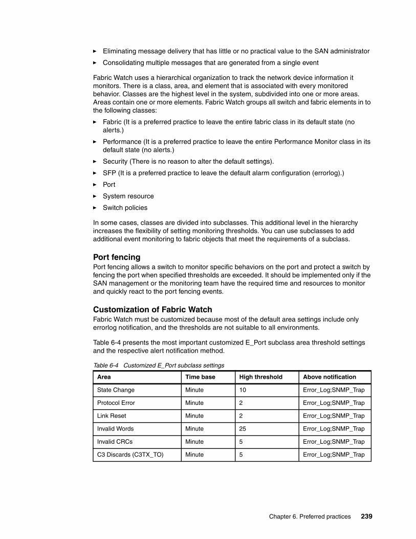
� Eliminating message delivery that has little or no practical value to the SAN administrator
� Consolidating multiple messages that are generated from a single event
Fabric Watch uses a hierarchical organization to track the network device information it monitors. There is a class, area, and element that is associated with every monitored behavior. Classes are the highest level in the system, subdivided into one or more areas. Areas contain one or more elements. Fabric Watch groups all switch and fabric elements in to the following classes:
� Fabric (It is a preferred practice to leave the entire fabric class in its default state (no alerts.)
� Performance (It is a preferred practice to leave the entire Performance Monitor class in its default state (no alerts.)
� Security (There is no reason to alter the default settings).
� SFP (It is a preferred practice to leave the default alarm configuration (errorlog).)
� Port
� System resource
� Switch policies
In some cases, classes are divided into subclasses. This additional level in the hierarchy increases the flexibility of setting monitoring thresholds. You can use subclasses to add additional event monitoring to fabric objects that meet the requirements of a subclass.
Port fencingPort fencing allows a switch to monitor specific behaviors on the port and protect a switch by fencing the port when specified thresholds are exceeded. It should be implemented only if the SAN management or the monitoring team have the required time and resources to monitor and quickly react to the port fencing events.
Customization of Fabric WatchFabric Watch must be customized because most of the default area settings include only errorlog notification, and the thresholds are not suitable to all environments.
Table 6-4 presents the most important customized E_Port subclass area threshold settings and the respective alert notification method.
Table 6-4 Customized E_Port subclass settings
Area Time base High threshold Above notification
State Change Minute 10 Error_Log;SNMP_Trap
Protocol Error Minute 2 Error_Log;SNMP_Trap
Link Reset Minute 2 Error_Log;SNMP_Trap
Invalid Words Minute 25 Error_Log;SNMP_Trap
Invalid CRCs Minute 5 Error_Log;SNMP_Trap
C3 Discards (C3TX_TO) Minute 5 Error_Log;SNMP_Trap
Chapter 6. Preferred practices 239
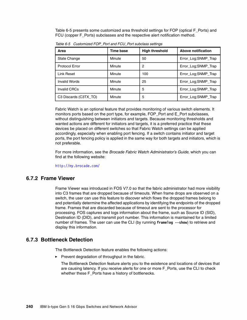
Table 6-5 presents some customized area threshold settings for FOP (optical F_Ports) and FCU (copper F_Ports) subclasses and the respective alert notification method.
Table 6-5 Customized FOP_Port and FCU_Port subclass settings
Fabric Watch is an optional feature that provides monitoring of various switch elements. It monitors ports based on the port type, for example, FOP_Port and E_Port subclasses, without distinguishing between initiators and targets. Because monitoring thresholds and wanted actions are different for initiators and targets, it is a preferred practice that these devices be placed on different switches so that Fabric Watch settings can be applied accordingly, especially when enabling port fencing. If a switch contains initiator and target ports, the port fencing policy is applied in the same way for both targets and initiators, which is not preferable.
For more information, see the Brocade Fabric Watch Administrator’s Guide, which you can find at the following website:
http://my.brocade.com/
6.7.2 Frame Viewer
Frame Viewer was introduced in FOS V7.0 so that the fabric administrator had more visibility into C3 frames that are dropped because of timeouts. When frame drops are observed on a switch, the user can use this feature to discover which flows the dropped frames belong to and potentially determine the affected applications by identifying the endpoints of the dropped frame. Frames that are discarded because of timeout are sent to the processor for processing. FOS captures and logs information about the frame, such as Source ID (SID), Destination ID (DID), and transmit port number. This information is maintained for a limited number of frames. The user can use the CLI (by running framelog --show) to retrieve and display this information.
6.7.3 Bottleneck Detection
The Bottleneck Detection feature enables the following actions:
� Prevent degradation of throughput in the fabric.
The Bottleneck Detection feature alerts you to the existence and locations of devices that are causing latency. If you receive alerts for one or more F_Ports, use the CLI to check whether these F_Ports have a history of bottlenecks.
Area Time base High threshold Above notification
State Change Minute 50 Error_Log;SNMP_Trap
Protocol Error Minute 2 Error_Log;SNMP_Trap
Link Reset Minute 100 Error_Log;SNMP_Trap
Invalid Words Minute 25 Error_Log;SNMP_Trap
Invalid CRCs Minute 5 Error_Log;SNMP_Trap
C3 Discards (C3TX_TO) Minute 5 Error_Log;SNMP_Trap
240 IBM b-type Gen 5 16 Gbps Switches and Network Advisor

� Reduce the time that it takes to troubleshoot network problems.
If you notice one or more applications slowing down, you can determine whether any latency devices are attached to the fabric and where. You can use the CLI to display a history of bottleneck conditions on a port. If the CLI shows above-threshold bottleneck severity, you can narrow the problem down to device latency rather than problems in the fabric.
You can use the Bottleneck Detection feature with other Adaptive Networking features to optimize the performance of your fabric.
Bottleneck detection requires some tuning on an environment by environment basis.
Parameter settingsField experience shows that the original strategy of enabling Bottleneck Detection with conservative values for latency thresholds almost always yields no results. There was a concern that aggressive values would result in Bottleneck Detection alert storms, but this has not been the case. Even the most aggressive values result in relatively few alerts being generated. As a result, it is now a preferred practice that the most aggressive settings are tried first and then backed off gradually if too many alerts are seen.
Table 6-6 shows the preferred parameter settings for Bottleneck Detection on FOS V.7.0.x.
Table 6-6 Bottleneck Detection preferred parameters for FOS V7.0.x
For the settings for previous FOS levels, see the latest Brocade SAN Fabric Resiliency Best Practices guide, which you can find at the following website:
http://my.brocade.com/
6.7.4 Credit loss
FOS V7.1 and later supports back-end credit loss detection back-end ports and core blades and on the Brocade 5300 and 6520 switches, although the support is slightly different on each device. Credit loss detection and recovery are enabled and disabled through the CLI by running bottleneckmon --cfgcredittools:
bottleneckmon --cfgcredittools -intport -recover onLrThresh
Parameter Conservativesetting
Normalsetting
Aggressivesetting
-time 300 60 5
-qtime 300 60 1
-lthresh 0.3 0.1 0.2
-cthresh 0.8 0.5 0.1
-lsubsectimethresh 0.8 0.5 0.5 (no less)
-lsubsecsevthresh 75 50 1
Chapter 6. Preferred practices 241

6.7.5 RAS log
The RAS log is the FOS error message log. Messages are organized by FOS component, and each one has a unique identifier and severity, source, and platform information and a text message.
A RAS log is available from each switch and director by running errdump, and RAS log messages can be forwarded to a syslog server for centralized collection.
6.7.6 Audit log
The Audit log is a collection of information that is created when specific events are identified on an IBM b-type platform. The log can be dumped by running auditdump, and audit data can also be forwarded to a syslog server for centralized collection.
Information is collected on many different events that are associated with zoning, security, trunking, FCIP, FICON, and others. Each release of the FOS provides more audit information.
6.7.7 SAN Health
SAN Health provides snapshots of fabrics showing information such as switch and firmware levels, connected device information, snapshots of performance information, zone analysis, and ISL fan-in ratios.
6.7.8 Design guidelines
You should implement some form of monitoring for each switch. Often, issues start out relatively benignly and gradually degrade into more serious problems. Monitoring the logs for serious and error severity messages helps you avoid many problems. Consider implementing to following items:
� Plan for a centralized collection of the RAS log, and perhaps the Audit log, through syslog. You can optionally filter these messages relatively easily through some simple Perl programs.
� IBM b-type platforms can generate SNMP traps for most error conditions. Consider implementing some sort of alerting mechanism through SNMP.
6.7.9 Monitoring and notifications
Error logs should be looked at regularly. Many users use combinations of syslog and SNMP with the Fabric Watch and the logs to maintain a close eye on the health of their fabrics. Network Advisor has many helpful features to configure and monitor your fabrics.
6.8 Scalability, supportability, and performance
IBM b-type products are designed with scalability in mind because most installations continue to expand, and that growth is supported by few restrictions. However, you should follow the same basic principles there were outlined in previous sections as the network grows.
242 IBM b-type Gen 5 16 Gbps Switches and Network Advisor

Evaluate the impact on topology, data flow, workload, performance, and, most importantly, redundancy and resiliency of the entire fabric any time one of the following actions is performed:
� Adding or removing initiators:– Changes in workload– Changes in provisioning
� Adding or removing storage: Changes in provisioning� Adding or removing switches� Adding or removing ISLs� Virtualization (workload and storage) strategies and deployments
If these design practices are followed when the network is deployed, then small incremental changes should not adversely impact the availability and performance of the network. However, if changes are ongoing and the fabric is not properly evaluated and updated, then performance and availability can be jeopardized. Here are some key points to cover when looking at the status of a production FC network:
� Review redundancy and resiliency, taking into account at least the following items:
– Are there at least two physically independent paths between each source and destination pair?
– Are there two redundant fabrics?
– Does each host connect to two different edge switches?
– Are edge switches connected to at least two different core switches?
– Are inter-switch connections composed of two trunks of at least two ISLs?
– Does each storage device connect to at least two different edge switches or separate port blades?
– Are storage ports provisioned such that every host has at least two ports through which it can access LUNs?
– Are redundant power supplies attached to different power sources?
– Are zoning and security policies configured to allow for patch/device failover?
� Reviewing performance requirements:
– Host-to-storage port fan-in/out ratios.
– Oversubscription ratios:
• Host to ISL
• Edge switch to core switch
• Storage to ISL
– Size of trunks.
– Routing policy and currently assigned routes: Evaluate actual usage for potential imbalances.
� Watching for latencies:
– Poor storage performance.
– Overloaded hosts or applications.
– Distance issues, particularly changes in usage (such as adding mirroring or too much workload).
– Deal with latencies immediately; they can have a profound impact on the fabric.
Chapter 6. Preferred practices 243

In summary, although IBM SANs are designed to allow for any-to-any connectivity, and they support provision-anywhere implementations, these practices can have an adverse impact on the performance and availability of the SAN if left unchecked. The network must be monitored for changes and routinely evaluated for how well it meets redundancy and resiliency requirements.
SupportabilitySupportability is a critical part of deploying a SAN. Follow the guidelines in this section to ensure that the data that is needed to diagnose fabric behavior or problems is collected. Although not all of these items are necessary, they are all pieces in the puzzle. You can never know which piece is needed, so having all of the pieces available is best.
� Configure Fabric Watch monitoring: Use Fabric Watch to implement proactive monitoring of errors and warnings, such as CRC errors, loss of synchronization, and high-bandwidth usage.
� Configure syslog forwarding: By keeping historical log messages and having all switch messages sent to one centralized syslog server, troubleshooting can be expedited and simplified. Forwarding switch error messages to one centralized syslog server and keeping historical log messages enables faster and more effective troubleshooting and provides a simple monitoring function.
� Back up switch configurations: Back up switch configurations on a regular basis so that you can restore switch configuration in case a switch must be swapped out or provide change monitoring functioning.
� Enable audit function: To provide audit functioning for the SAN, track which administrator made which changes, usage of multiple user accounts (or RADIUS), and configuration of change tracking or audit functions (along with use of errorlog/syslog forwarding).
� Configure multiple user accounts (LDAP/OpenLDAP or RADIUS): Make mandatory use of personalized user accounts part of the IT/SAN security policy so that user actions can be tracked. Also, restrict access by assigning specific user roles to individual users.
� Establish a test bed: Set up a test bed to test new applications, firmware upgrades, driver functions, and scripts to avoid missteps in a production environment. Validate functions and stability with rigorous testing in a test environment before deploying into the production environment.
� Implement a serial console server: Implement serial remote access so that switches can be managed even when there are network issues or problems during switch boot or firmware upgrades.
� Use aliases: Use “aliases,” which give switch ports and devices meaningful names. Using aliases to give devices meaningful names can lead to faster troubleshooting.
� Configure supportftp: Configure supportftp for automatic file transfers. The parameters set by this command are used by supportSave and traceDump.
� Configure a ntp server: To keep a consistent and accurate date and time on all the switches, configure switches to use an external time server.
� Disable a default zone: Set the default zoning mode to “No Access”.
� Enabling insistent domain ID: It is a preferred practice to set the domain ID to be insistent to make the domain ID insistent across reboots, power cycles, and failovers.
� Persistent Disable unused ports: If possible, unused ports should be persistently disabled.
� Disable E_Port capability for F_Ports: Ports that are connected to storage and host devices should have their E_PORT functioning persistently disabled.
244 IBM b-type Gen 5 16 Gbps Switches and Network Advisor

Chapter 7. Troubleshooting
This chapter describes the steps that you can take to ascertain the health of the storage area network (SAN) fabric and to troubleshoot problems. This chapter describes SAN Health, a powerful tool that allows you to collect data and analyze this data for potential issues. This chapter also describes the Advanced Performance Monitors, Diagnostic Features, gathering port information, and system messages.
7
© Copyright IBM Corp. 2014. All rights reserved. 245

7.1 SAN Health
Brocade SAN Health is a no-charge software utility that is designed to securely audit and analyze your SAN environment. To help optimize your SAN's performance, SAN Health automatically discovers critical fabric characteristics and reports their details in easy-to-understand Excel and Visio formats. In addition, SAN Health performs critical tasks, such as the following ones:
� Taking inventory of devices, switches, firmware versions, and fabrics� Capturing and displaying historical performance data� Comparing zoning and switch configurations against preferred practices� Assessing performance statistics and error conditions� Producing detailed graphical reports and diagrams
SAN Health gives you a powerful tool that helps you focus on optimizing your SAN rather than manually tracking its components. In fact, a wide variety of useful features make it easier for you to collect data, identify potential issues, and check your results over time.
To provide a comprehensive report about your SAN environment, SAN Health uses two main components:
� Data capture application � Back-end report processing engine
After SAN Health finishes the capture of switch diagnostic data, the back-end reporting process automatically generates a Visio topology diagram and a detailed snapshot report of your SAN configuration. This summary report contains information about the entire SAN and specific details about fabrics, switches, and individual ports. Other useful items in the report include alerts, historical performance graphs, and preferred practices. SAN Health delivers topology diagrams, comprehensive reports, detailed explanations, and more.
7.1.1 New features of SAN Health
SAN Health V3.2.7b includes the following new features:
� Supports Cisco MDS switches� Improved reporting for all Brocade m-series SAN solutions, including the Brocade Mi10k� The ability to audit switches that are managed by Brocade EFCM� Enhanced topology diagram layouts� More detailed diagnostic information can be obtained from switches� A redesign of the report content and layout� FICON enhancements for mainframe environments
7.1.2 Implementing SAN Health
This section explains how to download, install, and use SAN Health.
Installing Brocade SAN HealthTo install Brocade SAN Health, complete the following steps:
1. Go to the following link and download SAN Health Diagnostics Capture:
http://www.brocade.com/services-support/drivers-downloads/san-health-diagnostics/download_san_health.page
246 IBM b-type Gen 5 16 Gbps Switches and Network Advisor

2. Extract InstallSANHealth327b.zip and run InstallSANHealth327b.exe, accepting the defaults.
Using Brocade SAN Health Diagnostics CaptureAfter you have downloaded, extracted, and installed SAN Health Diagnostics Capture, you can run it by using the desktop icon. Then, complete the following steps:
1. Enter the site details.
2. Enter the Report Return details.
3. Name the SAN you are auditing.
4. Add switches by entering their IP addresses and login credentials.
5. Complete the Fabric details, enter the performance capture duration, and test the connectivity.
6. On the Switch Details tab, ensure that the switch login credentials are correct.
7. Select the Start audit tab and click Preflight check. If the preflight check did not pass, correct any errors and rerun the check until it passes. Normally, you get a “green smiley icon” if all the tests are OK.
8. The audit begins when you select Start Audit. SAN Health gathers data. How long this process takes depends on the capture performance data interval that you set on the Fabric tab. You can watch the progress of the tool as it completes the checks.
9. When this process completes, the output is an encrypted and compressed file that can be found in the C:\SAN Health Audits\ directory.
10.To complete the process, you must send the encrypted SAN Health file (.BSH) to the Brocade report generator. You have three choices to complete this task:
– Click Send the diagnostics data file via HTTPS.– Upload the file at https://my.brocade.com/upload/ReportGeneration.jsp.– Send the file as an email attachment to mailto:[email protected].
You receive a report generation notification email from the Brocade SAN Health Administrator and the report is available for download at the MyBrocade portal. The report contains a spreadsheet, a Visio file, and SHData files. This last file can be loaded by SAN Health Professional to perform advanced analysis.
7.1.3 SAN Health Professional
Brocade SAN Health Professional provides an easy-to-understand framework for analyzing SAN components and configuration data that is captured by the SAN Health Diagnostics Capture utility. It provides a straightforward, easy-to-navigate user interface for auditing SAN Health data captures, making it a valuable tool for SAN inventory tracking and change management activities. You can import up to two SAN Health Diagnostic Capture captures to SAN Health Professional for immediate, detailed analysis about any SAN component.
In addition to its standard data analysis and search capabilities, the SAN Health Professional framework supports optional add-on modules.
SAN Health Professional provides a straightforward, easy-to-navigate user interface for auditing SAN Health data captures, making it a valuable tool for inventory tracking and change management activities. Organizations can import up to two SAN Health captures to SAN Health Professional for immediate, detailed analysis about any component.
Chapter 7. Troubleshooting 247
To enable the highest level of flexibility, SAN Health Professional provides extensive searching and filtering capabilities. Searches can be broad (for example, a single search string such as “HBA” or “CHIPID”) or precise. Precision searching narrows the search to any combination of attribute names, devices, ports, switches, directors, fabrics, aliases, zones, or configurations.
Installing Brocade SAN Health ProfessionalTo install Brocade SAN Health, complete the following steps:
1. Go to the following link and download SAN Health Professional:
http://www.brocade.com/services-support/drivers-downloads/san-health-diagnostics/dowload_sanHealth_pro.page
2. Extract InstallSANHealthPro_1006.zip and run InstallSANHealthPro.exe, accepting the defaults.
3. Start Brocade SAN Health Professional.
4. Load up to two of the SHData files that are provided in the report that is generated automatically and perform the analysis.
7.2 Advanced Performance Monitoring
Advanced Performance Monitoring provides the following monitors:
� End-to-End monitors (EE monitors) measure the traffic between a host/target pair.
� Frame monitors measure the traffic that is transmitted through a port with specific values in the first 64 bytes of the frame.
� Top Talker monitors measure the flows that are major consumers of bandwidth on a switch or port.
7.2.1 End-to-End monitoring
Use End-to-End (EE) monitoring when you want to monitor throughput between a pair of devices. EE monitoring counts the number of words in Fibre Channel frames for a specified Source ID (SID) and Destination ID (DID) pair.
To enable EE monitoring, you must configure an EE monitor on a port, specifying the SID-DID pair (in hexadecimal). The monitor counts only those frames with matching SID and DID.
Each SID or DID has the following three fields:
� Domain ID (DD)� Area ID (AA)� AL_PA (PP)
For example, the SID 0x118a0f denotes DD 0x11, AA 0x8a, and AL_PA 0x0f.
248 IBM b-type Gen 5 16 Gbps Switches and Network Advisor

An EE monitor includes these counts:
� RX_COUNT: Words in frames that are received at the port. For frames that are received at the port with the EE monitor installed, the RX_COUNT is updated if the frame SID is the same as the SID in the monitor and the frame DID is the same as the DID in the monitor.
� TX_COUNT: Words in frames that are transmitted from the port. For frames that are transmitted from the port with the EE monitor installed, TX_COUNT is updated if the frame DID is the same as the SID in the monitor and the frame SID is the same as the DID in the monitor.
Supported port configurations for EE monitorsYou can configure EE monitors on F_Ports and, depending on the switch model, on E_Ports. The following platforms support EE monitors on E_Ports:
� IBM System Networking SAN24B-5� IBM System Networking SAN48B-5� IBM System Networking SAN96B-5� IBM System Networking SAN384B-2� IBM System Networking SAN768B-2
Identical EE monitors cannot be added to the same port. Two EE monitors are considered identical if they have the same SID and DID values after applying the end-to-end mask.
An EE monitor and a port Top Talker monitor cannot coexist on the same port.
Coexistence of EE monitors and Top Talker monitors on ports belonging to the same ASIC is not recommended because the statistics for the same flow going through ports on the same ASIC might be inaccurate.
Adding EE monitorsTo add EE monitors, using admin permissions, run the following command
perfaddeemonitor [slotnumber/]portnumber sourceID destID
EE monitoring looks at traffic on SID and DID pairs in any direction. That is, even if the SID is for a remote device, the traffic is monitored in both directions (the Tx and Rx counters are reversed).
The E_Port monitors are configured similar to the F_Port monitors, but the ingress and egress directions are reversed.
Deleting EE monitorsTo delete EE monitors, using admin permissions, first run perfMonitorShow to list the valid EE monitor numbers for a port. THen, run perfDelEEMonitor to delete a specific monitor.
If you do not specify which monitor number to delete, you are asked if you want to delete all entries.
Displaying EE monitor countersYou can use this procedure to display the EE monitors on a specified port. You can display either the cumulative count of the traffic that is detected by the monitors or a snapshot of the traffic at specified intervals.
Using admin permissions, run the following command:
perfmonitorshow --class monitor_class [slotnumber/]portnumber [interval]
Chapter 7. Troubleshooting 249

Managing EE monitoring through IBM Network AdvisorTo manage EE monitoring through IBM Network Advisor, open the Set End-to-End Monitors dialog box by clicking Monitor Performance End-to-End Monitors and follow the instructions that are provided in the IBM Network Advisor User Manual.
7.2.2 Frame monitoring
Frame monitoring counts the number of times a frame with a particular pattern is transmitted by a port, and generates alerts when thresholds are crossed. Frame monitoring is achieved by defining a filter, or frame type, for a particular purpose. The frame type can be a standard type (for example, a SCSI read command filter that counts the number of SCSI read commands that were transmitted by the port) or a user-defined frame type that is customized for your particular use. For a list of the standard, predefined frame types, see the fmMonitor command description in the Fabric OS Command Reference.
The maximum number of frame monitors and offsets per port depends on the platform. For more information, see the Fabric OS Administrator’s Guide.
In addition to the standard frame types, you can create custom frame types to gather statistics that fit your needs. To define a custom frame type, you must specify a series of offsets, bitmasks, and values.
Creating a frame monitorTo create a frame monitor, using admin permissions, run the following command:
fmmonitor --create frame_type -pat bit_pattern [-port port_list] [-highth value] [-action actions] [-timebase time_base] [-nosave]
The Fabric OS Command Reference manual contains practical examples about how to create frame monitors.
Deleting frame typesDeleting a frame type removes the entire configuration, including configured thresholds and associated actions. It also removes any frame monitors of the specified type from all ports. You can delete only user-defined frame types; you cannot delete the predefined frame types.
To delete a specific frame type, run fmMonitor --delete frame_type.
Adding frame monitors to a portIf the switch does not have enough resources to add a frame monitor to a port, then other frame monitors on that port might have to be deleted to free resources.
Note: The Advanced Performance Monitoring license is required to use the fmMonitor command. The monitoring function also requires the Fabric Watch license. When you configure actions and alerts through the fmMonitor command, Fabric Watch uses these values and generates alerts that are based on the configuration. If you do not have a Fabric Watch license, these values are ignored. For more information about using Fabric Watch, see the Fabric Watch Administrator’s Guide.
Virtual Fabrics considerations: Frame monitors are not supported on logical ISLs (LISLs), but are supported on ISLs and extended ISLs (XISLs).
250 IBM b-type Gen 5 16 Gbps Switches and Network Advisor
To add a frame monitor to one or more ports, using admin permissions, run fmMonitor --addmonitor.
The set of ports to be removed from monitoring is automatically saved to the persistent configuration unless you specify the -nosave option with the command.
Removing frame monitors from a portTo remove a specific monitor from one or more ports, run fmMonitor --delmonitor. The set of ports to be removed from monitoring is automatically saved to the persistent configuration unless you specify the -nosave option with the command.
Saving a frame monitor configurationWhen you assign or remove frame monitors on ports, the list of ports to be monitored is automatically saved persistently unless you specified the -nosave option.
To save the set of ports on which the frame type is monitored to the persistent configuration, using admin permissions, run fmMonitor --save.
Displaying frame monitorsTo display frame monitors, using admin permissions, run fmMonitor --show.
Managing Frame Monitoring through IBM Network AdvisorTo manage Frame Monitoring through IBM Network Advisor, open the Frame Monitor dialog box by clicking Monitor Fabric Watch Frame Monitor and follow the instructions that are provided in the IBM Network Advisor User Manual, found at:
http://www-01.ibm.com/support/docview.wss?uid=ssg1S7004661
7.2.3 Top Talker monitors
Top Talker monitors determine the flows (SID and DID pairs) that are the major users of bandwidth (after initial stabilization). Top Talker monitors measure bandwidth usage data in real time and relative to the port on which the monitor is installed.
Applications can use Top Talker monitors’ data to accomplish the following tasks:
� Reroute the traffic through different ports that are less busy, so as not to overload a port.� Alert you to the top-talking flows on a port if the total traffic on the port exceeds the
acceptable bandwidth consumption.
You can use Top Talker monitors to identify the SID and DID pairs that consume the most bandwidth and can then configure them with certain quality of service (QoS) attributes so they get proper priority.
The Top Talker monitor is based on SID and DID pairs and not WWNs. After Top Talker monitors are installed on a switch or port, they remain installed across power cycles.
Note: Initial stabilization is the time that is taken by a flow to reach the maximum bandwidth. This time varies depending on the number of flows in the fabric and other factors. The incubation period can be up to 14 seconds in the backbones, and up to 82 seconds in the fixed-port switches.
Chapter 7. Troubleshooting 251
Top Talker monitors support two modes: port mode and fabric mode.
� Port mode Top Talker monitor: A Top Talker monitor can be installed on a port to measure the traffic originating from the port and flowing to different destinations. You can configure Top Talker monitors on F_Ports and, depending on the switch model, on E_Ports. The following platforms support Top Talker monitors on E_Ports:
– IBM System Networking SAN24B-5– IBM System Networking SAN48B-5– IBM System Networking SAN96B-5– IBM System Networking SAN384B-2– IBM System Networking SAN768B-2
� Fabric mode Top Talker monitor: In fabric mode, Top Talker monitors are installed on all E_Ports in the fabric and measure the data rate of all the possible flows in the fabric (ingress E_Port traffic only). In fabric mode, Top Talker monitors can determine the top n bandwidth users on a given switch.
You can install Top Talker monitors in either port mode or fabric mode, but not both. A fabric mode Top Talker monitor and an EE monitor cannot be configured on the same fabric. You must delete the EE monitor before you configure the fabric mode Top Talker monitor.
Differences between Top Talker and EE monitorsEE monitors provide counter statistics for traffic flowing between a given SID and DID pair. Top Talker monitors identify all possible SID and DID flow combinations that are possible on a given port and provide a sorted output of the top talking flows. Also, if the number of flows exceeds the hardware resources, existing EE monitors fail to get real-time data for all of them; however, Top Talker monitors can monitor all flows for a given E_Port or F_Port.
Limitations of Top Talker monitorsConsider the following items when you use Top Talker monitors:
� Top Talker monitors cannot detect transient surges in traffic through a given flow.
� You cannot install a Top Talker monitor on a mirrored port.
� Top Talker monitors can monitor only 10,000 flows at a time.
� Top Talker monitors are not supported on VE_Ports, EX_Ports, and VEX_Ports.
� The maximum number of all port mode Top Talker monitors on an ASIC is 16. If Virtual Fabrics is enabled, the maximum number of all port mode Top Talker monitors on an ASIC is 8.
� If the ingress and egress monitor ports are configured on the same ASIC, F_Port Top Talker monitors show the flow from only one of the ports, either the ingress or the egress port, but not both.
Adding a Top Talker monitor to a port (port mode)To add a Top Talker monitor to a port (in port mode), using admin permissions, run perfttmon --add [egress | ingress] [slotnumber/]port.
Adding Top Talker monitors on all switches in the fabric (fabric mode)When fabric mode is enabled, you can no longer install Top Talker monitors on an F_Port unless you disable fabric mode. To accomplish this task, complete the following steps:
1. Connect to the switch and log in using an account with admin permissions.
2. Remove any EE monitors in the fabric. Fabric mode Top Talker monitors and EE monitors cannot both exist in the fabric.
252 IBM b-type Gen 5 16 Gbps Switches and Network Advisor
3. Run perfTTmon --add fabricmode.
The system responds with the following message:
Before enabling fabric mode, please remove all EE monitors in the fabric continue? (yes, y, no, n):
4. Enter y at the prompt to continue.
Top Talker monitors are added to E_Ports in the fabric and fabric mode is enabled. Any Top Talker monitors that were already installed on F_Ports are automatically uninstalled.
If EE monitors are present on the local switch, the command fails with the following message:
Cannot install Fabric Mode Top Talker because EE monitor is already present
If EE monitors are present on remote switches, the command succeeds; however, on the remote switches, fabric mode fails and a raslog message is displayed on those switches.
If a new switch joins the fabric, you must run perfTTmon --add fabricmode on that switch. The Top Talker monitor configuration information is not automatically propagated to the new switch.
Displaying the top n bandwidth-using flows on a port (port mode)To display the top n bandwidth-using flows on a port (in port mode), using admin permissions, run perfttmon --show [slotnumber/]port [n] [wwn | pid].
The output is sorted based on the data rate of each flow. If you do not specify the number of flows to display, then the command displays the top eight flows or the total number of flows, whichever is less.
Displaying the top talking flows for a given domain ID (fabric mode)To display the top talking flows for a given domain ID (in fabric mode), using admin permissions, run perfttmon --show dom domainid [n] [wwn | pid].
Fabric mode must be enabled for this option. The output is sorted based on the data rate of each flow. If you do not specify the number of flows to display, then the command displays the top eight flows or the total number of flows, whichever is less. The command can display a maximum of 32 flows.
Deleting a Top Talker monitor on a port (port mode)To delete a Top Talker monitor on a port (in port mode), using admin permissions, run perfttmon --delete [slotnumber/]port.
Deleting all the fabric mode Top Talker monitorsTo delete all the fabric mode Top Talker monitors, using admin permissions, run perfttmon --delete fabricmode.
All Top Talker monitors are deleted.
Managing Top Talker monitors through IBM Network AdvisorTo manage Frame Monitoring through IBM Network Advisor, open the Top talker Selector dialog box by clicking Monitor Performance Top Talkers and follow the instructions that are provided in the IBM Network Advisor User Manual, found at:
http://www-01.ibm.com/support/docview.wss?uid=ssg1S7004661
Chapter 7. Troubleshooting 253
7.3 Diagnostic features
The following sections show some of the more useful diagnostic features that you can use to gather relevant support information.
Diagnostic informationYou can run supportShow on the switch to dump important diagnostic and status information to the session screen, where you can review it or capture its data. If you are using a Telnet/SSH client, you might have to set up the client to capture the data before opening the session. Most information can be captured by running supportSave and downloading the information by FTP off the switch, but when you are collecting information from specialized commands such as supportShow, this information must be captured by using a Telnet/SSH client.
To save a set of files that customer support technicians can use to further diagnose the switch condition, run supportSave. The command prompts for an FTP server, packages the following files, and sends them to the specified server:
� The output of the supportShow command� The contents of any trace dump files on the switch� System message (RAS) logs
Switch statusTo display the overall status of the switch, including its power supplies, fans, and temperature, run switchStatusShow. If the status of any one of these components is either marginal or down, the overall status of the switch is also displayed as marginal or down. If all components have a healthy status, the switch displays a healthy status.
To modify the rules that are used to classify the health of each component, run switchStatusPolicySet. To view the rules, run switchStatusPolicyShow.
Using the SpinFab and portTest commandsThe spinFab command is an online diagnostic command to verify the ISL links between switches at the maximum speed. The verification is done by setting up the routing function in the hardware such that the test frames received by E_Port are retransmitted on the same E_Port. Several frames are then sent to the port that is attached to each active E_Port that is specified. These frames are special frames that never occur during normal traffic, and the default action for such frames is to route them back to the sender. These frames are circulated between switches until the test stops them. You can also run spinFab to test F_Ports, which requires a Brocade HBA with firmware version 2.1.1 or later.
The portTest command verifies the functional operation of the switch by sending frames from a port's transmitter, and looping the frames back through an external fiber cable into the same port's receiver. The test checks all switch components from the main board to the media, to the fiber cable, to the media of the devices and the switch, and back to the main board. This command supports E_Ports, F_Ports (must support ELS Echo), Report, and N->N loopback ports. In addition, on switches running FOS V6.4.0 and later, you can now use portTest on port configurations that previously caused non- specific test results or were skipped by portTest.
254 IBM b-type Gen 5 16 Gbps Switches and Network Advisor

Diagnostic Port (D_Port)D_Port mode allows you to convert a Fibre Channel port into a diagnostic port for testing link traffic, electrical loopbacks, and optical loopbacks between a pair of switches, a pair of Access Gateways, and an Access Gateway and a switch. The ports must use 10G or 16G Brocade-branded SFPs.
Support is also provided for running D_Port tests between a host bus adapter (HBA) and a switch. The test results that are reported can be useful in diagnosing various port and link problems.
The D_Port does not carry any user traffic, and is designed to run only specific diagnostic tests on it for identifying link-level faults or failures. Basically, to start a port in D_Port mode, you must configure both ends of the link between a pair of switches (or switches that are configured as Access Gateways), and you must disable the existing port before you can configure it as a D_Port.
After the ports are configured as D_Ports, the following basic test suite is run in the following order, depending on the SFPs that are installed:
1. Electrical loopback (with 16G SFP+ only)2. Optical loopback (with 16G SFP+ only)3. Link traffic (with 10G SFPs and 16G SFP+)4. Link latency and distance measurement (with 10G SFPs and 16G SFP+)
Here are the fundamentals of D_Port testing:
1. The user configures the ports on both ends of the connection.
2. After both sides are configured, a basic test suite is initiated automatically when the link comes online, conducting diagnostic tests in the following order:
a. Electrical loopbackb. Optical loopbackc. Link traffic
3. After the automatic test is complete, the user can view results (through CLI or GUI) and rectify issues (if any) that are reported.
4. The user can also start (and restart) the test manually to verify the link.
Enabling D_PortTo configure a basic D_Port diagnostic session between two switches, complete the following steps:
1. Disable Port 1 on Switch A by running portDisable [slot/]port:
switchA:admin> portdisable 1
2. Configure Port 1 on Switch A as a D_Port by running portCfgDport --enable [slot/]port:
switchA:admin> portcfgdport --enable 1
3. Repeat steps 1 and 2 for the corresponding port (in this example, Port 2) on Switch B:
switchB:admin> portdisable 2switchB:admin> portcfgdport --enable 2
4. Enable Port 1 on Switch A by running portEnable [slot/]port:
switchA:admin> portenable 1
Note: Electrical and optical loopback tests are not supported for ICLs.
Chapter 7. Troubleshooting 255

5. Enable Port 2 on Switch B by running portEnable [slot/]port:
switchB:admin> portenable 2
6. While the test is running, run portDportTest [slot/]port --show to view the test results.
7. To display a summary of the D_Port, run portDportTest [slot/]port with the --show all option.
8. Optional: If one of the switches reboots, or if the test does not complete on one of the switches, restart the test on both switches. Run portDportTest --stop and restart the test by running portDportTest --start on both switches.
For more information about the portDportTest and portCfgDport commands, see the Fabric OS Command Reference.
Disabling D_PortTo disable the D_Port diagnostic session that is described in “Enabling D_Port” on page 255, complete the following steps:
1. Disable Port 1 on Switch A by running portDisable 1 [slot/]port:
switchA:admin> portdisable 1
2. Disable the D_Port on Port 1 on Switch A by running portCfgDport --disable 1:
switchA:admin> portcfgdport --disable 1
3. Repeat steps 1 and 2 for Port 2 on Switch B:
switchB:admin> portdisable 2switchB:admin> portcfgdport --disable 2
4. Enable Port 1 on Switch A by running portEnable [slot/]port:
switchA:admin> portenable 1
5. Enable Port 2 on Switch B by running portEnable [slot/]port:
switchB:admin> portenable 2
Saving comprehensive diagnostic files to the serverTo save comprehensive diagnostic files to the server, connect to the switch, log in as the admin user, run supportSave -c, and respond to the prompts. The -c flag uses the FTP, SCP, or SFTP parameters that are saved by the supportFtp command. If this flag is omitted, you must specify the FTP, SCP, or SFTP parameters through command-line options or interactively. To display the current supportFTP parameters, run supportFtp (on a dual-CP system, run supportFtp on the active CP).
Scheduling technical support information collection through INAYou can capture technical support and event information for up to 50 devices. Technical SupportSave uses the built-in FTP, SCP, or SFTP server that is configured on the Management server to save data.
To capture technical support and event information, complete the following steps.
1. Click Monitor Technical Support Product/Host SupportSave. The Technical SupportSave dialog box opens.
2. Click the Schedule tab.
3. Select the Enable scheduled Technical Support Data check box.
4. Select how often you want the scheduled collection to occur from the Frequency list.
256 IBM b-type Gen 5 16 Gbps Switches and Network Advisor

5. Select the start date for the scheduled collection from the Start Date list. This list is only available when you select Weekly or Monthly from the Frequency list.
6. Select the time that you want the scheduled collection to begin from the Start Time Hour and Minute lists.
7. Click the SAN Products tab, if necessary, and complete the following steps. The Available SAN Products table displays the following information:
– All Levels: All discovered devices and ports as both text and icons.
– Name: The name of the available switch.
– Product Type: The type of product.
– Tag: The tag number of the device.
– Serial #: The serial number of the device.
– WWN: The switch port’s worldwide name.
– IP Address: The switch port’s IP address.
– Domain ID: The switch port’s top-level addressing hierarchy of the domain.
– Vendor: The hardware vendor’s name.
– Model: The name and model number of the hardware.
– Port Count: The total number of ports.
– Firmware: The firmware version.
– Location: The customer site location.
– Contact: The primary contact at the customer site.
– Description: A description of the customer site.
– State: The switch state, for example, online or offline.
– Status: The operational status of the switch, for example, unknown or marginal.
a. Right-click in the Available SAN Products table and select Expand All.
b. Select the switches that you want to collect data for in the Available SAN Products table and click the right arrow to move them to the Selected Products and Hosts table.
8. Click the Hosts tab and complete the following steps. The Available Hosts table displays the following information:
– Name: The name of the available host.
– IP Address: The host port’s IP address.
– Network Address: The network address of the host.
– Fabrics: The fabric of the host.
a. Right-click in the Available SAN Products table and select Expand All.
b. Select the products that you want to collect data for in the Available Hosts table and click the right arrow to move them to the Selected Products and Hosts table. The Selected Products and Hosts table displays the following information:
• IP Address: The IP address of the selected product or host.
• Name: The name of the selected product or host.
• WWN: The worldwide name of the selected product or host.
• Firmware Type: The type of firmware: FOS (Fabric OS).
Chapter 7. Troubleshooting 257

• Firmware version: The firmware version of the selected product or host.
• Support Save Credentials: Whether the product or host has SupportSave credentials or not.
9. Select how often you want to purge the support data from the Purge Support Data list.
10.Click OK on the Technical SupportSave dialog box.
Starting immediate technical support information collectionTo capture technical support and event information for specified devices, complete the following steps:
1. Click Monitor Technical Support Product/Host SupportSave. The Technical SupportSave dialog box displays
2. Click the Generate Now tab, if necessary
3. Click the SAN Products tab, if necessary, and complete the following steps:
a. Right-click in the Available SAN Products table and select Expand All.
b. Select the switches that you want to collect data for in the Available SAN Products table and click the right arrow to move them to the Selected Products and Hosts table. Technical SupportSave data for Fabric OS devices is saved to the following directory:
Install_Home\data\ftproot\technicalsupport\
4. Click the Hosts tab, if necessary, and complete the following steps:
a. Right-click in the Available Hosts table and select Expand All.
b. Select the hosts that you want to collect data for in the Available Hosts table and click the right arrow to move them to the Selected Products and Hosts table.
5. Click OK on the Technical SupportSave dialog box. The Technical SupportSave Status dialog box opens with the following details:
– Name: The name of the product.
– IP Address: The product’s IP address.
– Firmware Type: The type of product.
– Progress: The status of the support save. On products running FOS V7.0 or later, this field shows the percentage complete and is updated every minute. For Host products, and FOS products running Version 6.4 or earlier, this field cannot display the percentage (only displays whether it is “In Progress” or “Completed”).
– Status: The status of the support save, for example, Success or Failure.
6. Click Close on the Technical SupportSave Status dialog box.
7.4 Port information
Use the following instructions to view information about ports and to help diagnose whether your switch is experiencing port problems.
Viewing the status of a portTo view the status of a port, using admin permissions, run portShow [slot/] port, specifying the number that corresponds to the port you are troubleshooting.
258 IBM b-type Gen 5 16 Gbps Switches and Network Advisor

Displaying the port statisticsTo display the port statistics, using admin permissions, run portStatsShow.
Displaying a summary of port errors for a switchTo display a summary of port errors for a switch, run portErrShow. For more portErrShow command information, see the Fabric OS Command Reference, which you can find at the following website:
http://my.brocade.com/
Table 7-1 provides a description of the error types that are displayed by the portErrShow command.
Table 7-1 Error summary description
Here are what these errors mean in statistical terms:
� crc_err and enc_out errors together imply an SFP issue.
� enc_out errors on their own imply a cable/connector issue. This error can cause a performance problem because of buffer recovery.
� too_long or too_short errors indicate an unreliable link.
� disc_c3 relates to port congestion.
� loss_sig can be indicative of incompatible speeds between two points, can be caused by severe physical layer errors, or by devices being reset, such as server reboots.
Error type Description
frames tx Frames transmitted.
frames rx Frames received.
enc in Encoding errors inside frames.
crc err Frames with CRC errors.
crc g_eof CRC errors that occur on frames with good end-of-frame delimiters.
too shrt Frames shorter than minimum.
too long Frames longer than maximum.
bad eof Frames with bad end-of-frame delimiters.
enc out Encoding error outside of frames.
disc c3 Number of Class 3 frames discarded (Rx). This counter includes the sum of the following Class 3 discard counters that are reported by the portStatsShow command: er_rx_c3_timeout, er_tx_c2_timeout, er_c2_dest_unreach, and er_other_disc.For a description of these counters, run portStatsShow help.
link fail Link failures (LF1 or LF2 states).
loss sync Loss of synchronization.
loss sig Loss of signal.
frjt Frames rejected with F_RJT.
fbsy Frames busied with F_BSY.
Chapter 7. Troubleshooting 259

Clearing the error countersTo clear the error counters, run portStatsClear <slot/port>.
As a preferred practice, clear the error counters on a weekly basis to get a base line to evaluate the current error counters.
Quick health checkTable 7-2 shows a sequence of four FOS commands that allow you to perform a preliminary health check of your fabric.
Table 7-2 Steps for a basic and quick health check
7.5 Overview of system messages
This section describes the types of system messages and what to do with them.
System message typesFOS supports three types of system messages. A system message can be of one or more of the following types:
� RASLog messages� Audit log messages� First Failure Data Capture messages
RASLog messagesRASLog messages report significant system events (failure, error, or critical conditions) or information, and are also used to show the status of the high-level user-initiated actions. RASLog messages are forwarded to the console, to the configured syslog servers, and to the SNMP management station through the Simple Network Management Protocol (SNMP) traps or informs.
The errDump command shows the error log without pagination, and the errShow command shows the error log messages with pagination.
The system messages are documented in the Fabric OS Message Reference guide, which helps you diagnose and fix problems. You can find this guide at the following website:
http://my.brocade.com/
The messages are organized alphabetically by module name. A module is a subsystem in the FOS. Each module generates a set of numbered messages. For each message, the guide provides message text, probable cause, recommended action, and severity level. There may be more than one cause and more than one recommended action for any given message, but the guide describes the most probable cause and typical action that is recommended.
FOS command Description
switchstatusshow Run this command to display the overall status for a switch.
switchshow Run this command to display switch, blade, and port status information.
porterrshow Run this command to display an error summary for all ports.
sfpshow <slot>/<port> Run this command to display Small Form-factor Pluggable (SFP) transceiver information.
260 IBM b-type Gen 5 16 Gbps Switches and Network Advisor

Audit log messagesEvent auditing is designed to support post-event audits and problem determination that is based on high-frequency events of certain types, such as security violations, zoning configuration changes, firmware downloads, and certain types of fabric events. Audit messages that are flagged as AUDIT are not saved in the switch error logs. The switch can be configured to stream audit messages to the switch console and to forward the messages to specified syslog servers. The audit log messages are not forwarded to an SNMP management station. There is no limit to the number of audit events.
First Failure Data Capture messagesFirst Failure Data Capture (FFDC) is used to capture failure-specific data when a problem or failure is noted for the first time and before the switch reboots or trace and log buffers are wrapped. All subsequent iterations of the same error are ignored. This critical debug information is saved in nonvolatile storage and can be retrieved by running supportSave. The FFDC data is used for debugging or analyzing the problem. FFDC is intended for use by Brocade technical support.
Chapter 7. Troubleshooting 261

262 IBM b-type Gen 5 16 Gbps Switches and Network Advisor

Related publications
The publications that are listed in this section are considered suitable for a more detailed discussion of the topics that are covered in this book.
IBM Redbooks
The following IBM Redbooks publications provide additional information about the topic in this document. Some publications referenced in this list might be available in softcopy only.
� IBM SAN and SVC Stretched Cluster and VMware Solution Implementation, SG24-8072
� IBM SAN Volume Controller Stretched Cluster with PowerVM and PowerHA, SG24-8142
� IBM SAN Volume Controller and IBM FlashSystem 820: Best Practices and Performance Capabilities, REDP-5027
� IBM Storwize V7000 and SANSlide Implementation, REDP-5023
� IBM System Storage SAN Volume Controller Best Practices and Performance Guidelines, SG24-7521
� Implementing the IBM SAN Volume Controller and FlashSystem 820, SG24-8172
� Implementing the IBM Storwize V3700, SG24-8107
� Implementing the IBM Storwize V5000, SG24-8162
� Implementing the IBM Storwize V7000 Unified, SG24-8010
� Implementing the IBM Storwize V7000 V6.3, SG24-7938
� Implementing the IBM System Storage SAN Volume Controller V6.3, SG24-7933
� Introduction to Storage Area Networks and System Networking, SG24-5470
� Real-time Compression in SAN Volume Controller and Storwize V7000, REDP-4859
You can search for, view, download, or order these documents and other Redbooks, Redpapers, Web Docs, draft and additional materials, at the following website:
ibm.com/redbooks
Help from IBM
IBM Support and downloads
ibm.com/support
IBM Global Services
ibm.com/services
© Copyright IBM Corp. 2014. All rights reserved. 263

264 IBM b-type Gen 5 16 Gbps Switches and Network Advisor

(0.5” spine)0.475”<
->0.873”
250 <->
459 pages
IBM b-type Gen 5 16 Gbps Sw
itches and Network Advisor
IBM b-type Gen 5 16 Gbps Sw
itches and Netw
ork Advisor
IBM b-type Gen 5 16 Gbps Sw
itches and Netw
ork Advisor
IBM b-type Gen 5 16 Gbps Sw
itches and Network Advisor

IBM b-type Gen 5 16 Gbps Sw
itches and Netw
ork Advisor
IBM b-type Gen 5 16 Gbps Sw
itches and Netw
ork Advisor

®
SG24-8186-00 ISBN 0738439231
INTERNATIONAL TECHNICALSUPPORTORGANIZATION
BUILDING TECHNICAL INFORMATION BASED ON PRACTICAL EXPERIENCE
IBM Redbooks are developed by the IBM International Technical Support Organization. Experts from IBM, Customers and Partners from around the world create timely technical information based on realistic scenarios. Specific recommendations are provided to help you implement IT solutions more effectively in your environment.
For more information:ibm.com/redbooks
®
IBM b-type Gen 5 16 Gbps Switches and Network Advisor
Learn about the new features of the IBM b-type Gen 5 16 Gbps switches
Read about IBM Network Advisor and Fabric Vision
Learn about preferred practices and troubleshooting tips
IBM System Storage Gen 5 fabric backbones are among the industry's most powerful Fibre Channel switching infrastructure offerings. They provide reliable, scalable, and high-performance foundations for mission-critical storage. These fabric backbones also deliver enterprise connectivity options to add support for IBM FICON connectivity, offering a high-performing and reliable FICON infrastructure with fast and scalable IBM System z servers.
Designed to increase business agility while providing nonstop access to information and reducing infrastructure and administrative costs, Gen 5 Fibre Channel fabric backbones deliver a new level of scalability and advanced capabilities to this robust, reliable, and high-performance technology.
Although every network type has unique management requirements, most organizations face similar challenges managing their network environments. These challenges can include minimizing network downtime, reducing operational expenses, managing application service level agreements (SLAs), and providing robust security. Until now, no single tool could address these needs across different network types.
To address this issue, the IBM Network Advisor management tool provides comprehensive management for data, storage, and converged networks. This single application can deliver end-to-end visibility and insight across different network types by integrating with Fabric Vision technology; it supports Fibre Channel SANs, including Gen 5 Fibre Channel platforms, IBM FICON, and IBM b-type SAN FCoE networks. In addition, this tool supports comprehensive lifecycle management capabilities across different networks through a simple, seamless user experience.
This IBM Redbooks publication introduces the concepts, architecture, and basic implementation of Gen 5 and IBM Network Advisor. It is aimed at system administrators, and pre- and post-sales support staff.
Back cover