Embed Size (px)
Citation preview

SANDIA REPORTSAND2001-2901Unlimited ReleasePrinted October 2001
Icarus: A 2-D Direct Simulation MonteCarlo (DSMC) Code for Multi-ProcessorComputers
User's Manual - v 10.0
Timothy J. Bartel, Steve Plimpton, and Michael A. Gallis
Prepared bySandia National LaboratoriesAlbuquerque, New Mexico 87185 and Livermore, California 94550
Sandia is a multiprogram laboratory operated by Sandia Corporation,a Lockheed Martin Company, for the United States Department ofEnergy under Contract DE-AC04-94AL85000.
Approved for public release; further dissemination unlimited.

Issued by Sandia National Laboratories, operated for the United States Departmentof Energy by Sandia Corporation.
NOTICE: This report was prepared as an account of work sponsored by an agencyof the United States Government. Neither the United States Government, nor anyagency thereof, nor any of their employees, nor any of their contractors,subcontractors, or their employees, make any warranty, express or implied, orassume any legal liability or responsibility for the accuracy, completeness, orusefulness of any information, apparatus, product, or process disclosed, or representthat its use would not infringe privately owned rights. Reference herein to anyspecific commercial product, process, or service by trade name, trademark,manufacturer, or otherwise, does not necessarily constitute or imply its endorsement,recommendation, or favoring by the United States Government, any agency thereof,or any of their contractors or subcontractors. The views and opinions expressedherein do not necessarily state or reflect those of the United States Government, anyagency thereof, or any of their contractors.
Printed in the United States of America. This report has been reproduced directlyfrom the best available copy.
Available to DOE and DOE contractors fromU.S. Department of EnergyOffice of Scientific and Technical InformationP.O. Box 62Oak Ridge, TN 37831
Telephone: (865)576-8401Facsimile: (865)576-5728E-Mail: [email protected] ordering: http://www.doe.gov/bridge
Available to the public fromU.S. Department of CommerceNational Technical Information Service5285 Port Royal RdSpringfield, VA 22161
Telephone: (800)553-6847Facsimile: (703)605-6900E-Mail: [email protected] order: http://www.ntis.gov/ordering.htm
Icarus: A 2-D Direct Simulation Monte Carlo (DSMC) Code for Multi-Processor Computers
User’s Manual - v 10.0
Timothy J. Bartel+
Computational Physics and Sim. Frameworks Department (9232)
Steve PlimptonParallel Computational Sciences Department (9233)
Michael A. GallisPlasma and Aerosol Department (9117)
Sandia National LaboratoriesP.O. Box 5800
Albuquerque, NM 87185-0626 USA
ABSTRACTIcarus is a 2D Direct Simulation Monte Carlo (DSMC) code which has been optimized for the par-
allel computing environment. The code is based on the DSMC method of Bird[11.1] and models fromfree-molecular to continuum flowfields in either cartesian (x, y) or axisymmetric (z, r) coordinates.Computational particles, representing a given number of molecules or atoms, are tracked as they havecollisions with other particles or surfaces. Multiple species, internal energy modes (rotation andvibration), chemistry, and ion transport are modelled. A new trace species methodology for collisionsand chemistry is used to obtain statistics for small species concentrations. Gas phase chemistry ismodelled using steric factors derived from Arrhenius reaction rates or in a manner similar to conti-uum modelling. Surface chemistry is modelled with surface reaction probabilities; an optional sitedensity, energy dependent, coverage model is included. Electrons are modelled by either a localcharge neutrality assumption or as discrete simulational particles. Ion chemistry is modelled withelectron impact chemistry rates and charge exchange reactions. Coulomb collision cross-sections areused instead of Variable Hard Sphere values for ion-ion interactions. The electro-static fields caneither be: externally input, a Langmuir-Tonks model or from a Green’s Function (Boundary Element)based Poison Solver. Icarus has been used for subsonic to hypersonic, chemically reacting, andplasma flows.
The Icarus software package includes the grid generation, parallel processor decomposition, post-processing, and restart software. The commercial graphics package, Tecplot, is used for graphics dis-play. All of the software packages are written in standard Fortran.
+ [email protected], (505)844-0124
SAND2001-2901Unlimited Release
Printed October 2001


Acknowledgments:
The authors would like to thank several people who contributed to this work, either by their directtechnical input, as ‘friendly’ users, or by their funding support. We first would like to thankWahid Hermina, Sandia National Labs (SNL), for both his technical insight and his support ofthis project, George Davidson, SNL, for early discussions on parallelizing the DSMC technique,and Jeff Payne, SNL, for his help with the postprocessing packages. The support from SudipDosanjh for the extensive use of the parallel computing facilities at Sandia and his help in ouracquisition of our own 1024 processor nCUBE is greatly appreciated. Robert Cochran, SandiaNational Labs, allowed us to freely use his finite element shape function routines in the initializa-tion code so that both function values and gradients could be obtained across region interfaces.Merle Riley, Mary Hudson and Matt Hopkins (all SNL) contributed to the addition of the Bound-ary Element Method formulation of the Poisson solver into Icarus. Justine Johannes (SNL) addednew surface chemistry models and the Chemkin file interface into Init2d. We also thank the fol-lowing people at Sandia National Labs who provided feedback in various stages of the codedevelopment and evolution: Don Potter, David Sears, Todd Sterk, Justine Johannes, Seung Choi,Rick Buss and Yvette Castro. Professor Demetre Economou, University of Houston, did his sab-batical leave at Sandia and contributed to the plasma modelling portion of the code. Nadeem Alvi,SEMATECH, provided both project support and precipitated our interactions with microelectron-ics equipment suppliers or end users. We thank Paul Shufflebotham and Vikram Singh, Novellus,for struggling through early versions of Icarus and for taking experimental data on their system tovalidate the code. We thank Tom Furlanni (SUNY-Buffalo) for his work on species weighting andVSS modelling and Penny Marriott for her work on the Maximum Entropy Model for post-colli-sion internal energy partitioning and chemical reactions. Feedback by Chris Shelton (3M), JamesGroves and Derek Haas (University of Virginia), and Ken Tatum (AEDC) have extended thecapabilities of Icarus. Ken also helped debug Icarus for a SGI-Origin system. We finally thankGraeme Bird, the developer of the DSMC method, for his insight during the early development ofthis code.
A PDF version of this manual (with color images) is available for downloading; please contact thefirst author for more information. PDF versions of the papers in section 12 are also available fordownloading. Please contact the first author about availability of the code.

Table of Contents
1.0 Direct Simulation Monte Carlo (DSMC): Background 11.1 Method.................................................................................................... 11.2 Grid Characteristics ................................................................................ 21.3 Cell and Species Weighting ................................................................... 31.4 Elastic Scattering Cross Section............................................................. 41.5 Internal Energy Exchange ...................................................................... 41.6 BGK........................................................................................................ 51.7 Plasma Features ...................................................................................... 51.8 Code Validation...................................................................................... 71.9 Computer Platforms ............................................................................... 71.10 Source Code Control ............................................................................ 7
2.0 Overall Code Structure 8
3.0 init2d - Icarus Preprocessor Program Description 103.1 Overview .............................................................................................. 103.2 init2d Code Description........................................................................ 103.3 Grid Characteristics .............................................................................. 113.4 Input File Description (geometry.inp).................................................. 113.5 Species File Description (spec) ............................................................ 293.6 Inlet File Description (inlet) ................................................................. 323.7 Surface Boundary Condition File (surfbc) ........................................... 353.8 Cross Section File (cross_section) ...................................................... 423.9 Gas Phase Chemistry File (chem or chem.asc) .................................... 443.10 Diagnostic Messages .......................................................................... 58
4.0 decomp2d - Decomposition Code Description 59
5.0 icarus - Code and Command File (dsmc.in) Description 605.1 icarus Command List Summary ........................................................... 615.2 Icarus Command Descriptions ............................................................. 655.3 Example dsmc.in Files ......................................................................... 835.4 Diagnostic Messages ............................................................................ 85
6.0 restart2d - Code Description 87
7.0 regrid2d - Code Description 89
8.0 Postprocessing Codes 918.1 Macroscopic Cell Information (post2d) ............................................... 928.2 Surface Information (surface2d) .......................................................... 958.3 Wafer Information (waferxy2d) ........................................................... 968.4 Cell Convergence Statistics (stat2d)..................................................... 98

9.0 Install/Compile Software 999.1 Make files ............................................................................................. 999.2 param.h and init2d.h files ................................................................... 1019.3 MPI ..................................................................................................... 104
10.0 Miscellaneous Information 10510.1 Important Relationships................................................................... 10510.2 Chemical Species Database. ............................................................. 106
11.0 References 110
12.0 Papers 1111
13.0 Sample Problems 11213.1 ICF Sphere ........................................................................................ 11213.2 Wedge ............................................................................................... 12013.3 AIAA V&V Spherically Blunted Bi-Conic (reference 12.9) ........... 12313.4 Plasma Charge Test .......................................................................... 12713.5 Plasma Screen (Ion Accelerator) ...................................................... 13313.6 Micro-Gyroscope .............................................................................. 14413.7 Collisional Test in a Closed Box ...................................................... 14713.8 MBF Expansion Chamber (reference paper 12.3) ............................ 15113.9 NO Nozzle Expansion and Data Comparison (reference paper 12.2) 16013.10 NO Vibrational Relaxation (Time Dependent)............................... 16813.11 Ion Accelerator ............................................................................... 174
14.0 Distribution 176

1.0 Direct Simulation Monte Carlo (DSMC): Background
1.1 MethodDSMC is a method for the direct simulation of rarefied gas flows[11.1]. The method as-
sumes that the gas is a dilute gas; that is, binary collisions dominate the molecular interactions.The flow domain is first divided into a number of cells. The cell size is determined by the localmean free path, λ,; a cell size ~ λ/3 is typically recommended. Unlike CFD grids with mesh or-thogonality and one-to-one cell side correspondence constraints, the DSMC grid system servesonly to identify a volume for choosing collision partners and for obtaining sampling statistics. Theflow field is simulated using a number of computational particles (some 107particles are not atyp-ical for runs on massively parallel supercomputers). Particles consist of all kinds of species suchas radicals, ions, and molecules. The species type, spatial coordinates, velocity components, inter-nal energy partitioning, and weight factor of each computational particle are stored. As the parti-cles move through the domain, they collide with one another and with surfaces. New particlesmay be added at specified inlet port locations, and particles may be removed from the simulationdue to chemical reactions or through the pumping ports. Since this is a statistical method in whichthe system evolves in a time-like manner, a steady-state solution is then an ensemble average of anumber of solution time steps (snapshots of the system) after the flow field has reached a steady-state. Icarus can also be run in a time accurate mode to model unsteady problems.
The basic premise of DSMC is that the motion of simulated particles can be decoupledfrom their collisions over a time step. The size of the time step is selected to be a small fraction ofthe mean collision time, or a fraction of the transit time of a molecule through a cell (similar to anexplicit CFL constraint). During the motion phase, particles move in free molecular motion ac-cording to their starting velocity and any body forces acting on the particles (for example theLorentz force on charged species). During this phase, particles may cross cell boundaries, collidewith walls and undergo surface chemistry, or exit the flow field. During the collision phase, ran-dom collision pairs are selected from within each cell regardless of the position of the particleswithin the cell. The no-time-counter (NTC) technique [11.3], is used to determine the computa-tional particle collision frequency. The number of pairs to be selected from a given cell at a timestep is
# pairs = 1/2 N N Fn (σTCr)max ∆t / Vwhere N is the number of computational particles in the cell, Fn the number of real particles persimulated one, (σTCr)max is the maximum of the product of the total cross-section and relative ve-locity for the pairs in the cell and V the cell volume. The pair collision is then computed with aprobability (σTCr) / (σTCr)max. This technique does not have the disadvantages of the older timecounter (TC) method while maintaining computational efficiency, i.e., the simulation time is pro-portional to the number of molecules. This is a great advantage of DSMC as compared to otherparticle simulation methods such as molecular dynamics. Also, the NTC method allows for un-steady flows to be simulated in a time accurate manner. A collision limiter model is used to im-prove computational performance at high pressures. The model simply limits the number ofcollisions in a cell to a multiple of the number of actual collisions. This model has been shown toreproduce inviscid flow fields and has been used to model high pressure (2 atm) nozzle expan-sions into a vacuum.
1

Direct Simulation Monte Carlo (DSMC): Background
Although only two position coordinates (r, z) of each simulated particle are stored, colli-sions are handled as three dimensional events to correctly conserve momentum transfer. The mo-lecular model used for collision cross sections is the variable hard sphere (VHS) model [11.1].According to this model, the collision cross section σij depends on the relative speed (energy) ofthe colliding partners Ec as
σij = Aij Ec−ω
where Aij is a constant and ω = s − 0.5, with s the exponent of the dependence of the coefficient ofviscosity on temperature. The chief advantage of the VHS model is that, although the collision di-ameter is allowed to vary with the relative speed (unlike the constant cross section hard spheremodel), when a collision does occur, the post-collision velocity components are computed as if itwere a hard sphere collision; that is, isotropic scattering in the center of mass frame of reference.
The DSMC technique can easily model internal energy modes: rotational and vibrationalenergies. The phenomenological Borgnakke and Larsen [11.2] model is used to determine thepost-collision internal energy partitioning given the number of internal degrees of freedom ofeach species. This is a harmonic oscillator model which drives the post-collision energy distribu-tion towards equilibrium. Recently, Marriott[11.5] and Gallis[11.6] has applied the Maximum En-tropy strategy for particle systems to obtain this energy distribution; unfortunately, the complexchemical species in typical manufacturing plasma etch systems are poorly characterized so typi-cally only translational nonequilibrium is modelled. Both models are included in the code.
Gas phase chemistry consists of six models: elastic gas reaction, charge exchange withfunctional cross-section fit, charge exchange using the model of Rapp and Frances, electron im-pact reactions for ionization or neutralization reactions, Arrhenius equation based continuum re-action modelling and inelastic electron impact reactions for the electron energy equation. Elasticcollision gas phase chemistry is modelled using steric factors derived from Arrhenius reactionrates. That is, the chemical reaction probability given a particle collision is determined assuming alocal Maxwellian distribution to convert the rate to a energy dependent probability. Charge ex-change reactions model the exchange of both energy and momentum between neutral and chargedspecies. Electron chemistry models electron impact chemistry using energy dependent rates andlocal electron number density and temperature. These rates are converted into a total reactionprobability. That is, a probability which includes both collision and reaction rates. Surface chem-istry is modelled with surface reaction probabilities; a optional, energy dependent, site coveragedependent model can also be used. The grid generation/preprocessor code, init2d, will input gasphase chemistry input in either a simple asci format or the standard CHEMKIN format.
1.2 Grid CharacteristicsIcarus uses a multi-block system of algebraic meshes to define the computational domain.
The grid is generated using the input processor program, init2d. This simple grid system allowsgreat flexibility for capturing local high gradient regions without excessively griding the entiredomain because there is no requirement for side correspondence between regions. See the paperby Bartel and Plimpton in Section 12.1 for more details.
2

Direct Simulation Monte Carlo (DSMC): Background
As mentioned before, the key assumption in DSMC is that particle transport is de-coupledfrom particle-particle interaction. Therefore particles move without collisions for a specified timestep, and then collision partners are chosen probabilistically from within a defined grid cell. Im-plementation of this method requires that the cell sizes and the time step be chosen carefully; par-ticles should not travel longer than the mean free path(λ) in a time step and the unit cell should besized approximately less than λ. The Knudsen number (Kn) and the Courant number (CFL) arequality metrics for the cell size and the time step:
(Kn > 1) = λ / cell length (CFL < 1) = particle velocity / (cell length / time step)
The cell Kn and CFL numbers are output from the DSMC code in the cell.* file and areused to verify that the particle transport assumptions were obtained.
1.3 Cell and Species WeightingIcarus uses several strategies to obtain sufficient statistics for both local regions of dispar-
ate densities and for ‘trace’ species which have a very small mole fraction. First, each grid cell hasa ‘weight’ which is simply used to spatially adjust the global or input ratio of real-to-computation-al particles. This ‘cell weight’ is initially proportional to the cell volume; this results in an equalnumber of computational particles per cell for a uniform initial density. As the simulationprogresses, the number of particles in a given cell can become extremely large due to either chem-ical events or mass injection into the system. The ‘cell adaption’ logic of Icarus dynamically ‘ad-justs’ the cell weight to maintain an upper bound on the number of computational particles percell. Thus the user can be assured of sufficient statistics without a few cells with an unreasonablenumber of particles. This feature is transparent to the user.
Species weighting is another method which is used to increase the sampling statistics forthe simulation. In this strategy, species which occur in small, trace amounts have a lower ‘compu-tational worth’ than do other species. For example, in low density plasma systems, the ionizationfraction is very small: < 0.1%. Thus, the neutral species will have a single weight of 1010 mole-cules or atoms per computational particle while the ions which occur in trace amounts will have aweight of 106 ions per computational particle. The code is limited to two species weight multipli-ers: 1.0 for the base or full case and a number less than 1.0 for all the trace species.
3

Direct Simulation Monte Carlo (DSMC): Background
1.4 Elastic Scattering Cross SectionThe Variable Hard Sphere (VHS) model treats each molecule as a fixed diameter sphere
with isotropic scattering. The VHS model employs the simple isotropic scattering law of the hardsphere model but accounts for the temperature dependence of the collision cross section by use ofa single parameter which may be determined from the viscosity temperature dependence
where is the collision cross section at the reference temperature, , and T is the kinetictemperature of the collision partners. The VHS parameter, is related to the temperature expo-nent of viscosity, s
as ; where η is the viscosity and subscript o denotes the reference temperature and vis-cosity (see ref. [11.1])
A database of viscosity index, ω, and molecular diameters at the reference temperature forapproximately 150 species has been compiled and given in Chapter 10.2. Curve fits to viscosity ofspecies not listed can be used to obtain s (the slope) and therefore ω.
Icarus contains a method to extend the computationally efficient pressure range to higherpressures. A collision limiter model is used: the number of computational collisions per computa-tional particle in a time step is constrained. This method has been shown to reproduce inviscidflow systems. The enclosed AIAA paper by Bartel, Sterk, Payne, et.al. (Section 12.3) contains thedetails and method comparisons.
1.5 Internal Energy ExchangeIn a typical application the particle simulators may possess internal degrees of freedom,
rotational, vibrational and electronic. The most common application is that of a particle with 2 ro-tational and 2 vibrational degrees of freedom, such as oxygen and nitrogen molecules. One way todeal with internal energy exchange is to define cross sections for all the possible allowable transi-tions. However, for most cases the number of states that needs to be included is so large that thisapproach is not practical. In DSMC the model that has been almost universally used since its in-troduction on 1974 is the phenomenological model of Borgnakke and Larsen (see Bird chapter 5[11.1]) and its variants. According to this model the relaxation process is modeled by assumingthat only a fraction of the collisions is inelastic.
The particular Borgnakke and Larsen method used in Icarus is the serial application of themethod. According to this, energy is partitioned in a serial fashion, starting with any mode anddistributing energy between that mode and an energy pool that contains all the undistributed colli-sion energy. For more details about the method the reader is referred to Bird’s monograph[11.1].Icarus offers the option of treating the vibrational mode in a quantized mode following the har-monic oscillator model. The parameters for the harmonic oscillator model for some gases are giv-
σ σrefT
Tref----------- ω–
=
σref Trefω
η η oT
To------ s
=
s ω 12---+=
4

Direct Simulation Monte Carlo (DSMC): Background
en in Appendix 1 of Bird’s monograph[11.1]. The relaxation parameters can be defined to beeither constant or a function of the total collision energy (“collision temperature”). Since there isno universally accepted model for the relaxation rate, for the particular case of nitrogen flowIcarus offers the option of a temperature dependent relaxation rate. In the general case this is to beconsidered as a place holder and if gases other than nitrogen need to be simulated the appropriaterelaxation rates need to be added to the code.
1.6 BGKIcarus incorporates a method to perform collisions in a collective manner. The method is
based on a simplified version of the Boltzmann equation the BGK method. The application andadaptation of the BGK method to DSMC is detailed in AIAA 2000-2360 (Section 12.10), where itwas found to be in good agreement with the standard DSMC collision algorithm. It should be not-ed that currently the method is only applicable to monatomic gases. Future extensions of themethod will include the internal degrees of freedom.
1.7 Plasma FeaturesIcarus contains several additional models for the simulation of ionized gases. First, the
electrons can be considered to be in local charge neutrality (LCN) with the ions (usually validwhen the Debye Length is much smaller than a characteristic cell length) or can be modelled asdiscrete particles in a similar fashion as a PIC plasma code. The LCN assumption can generally beused in geometries where the sheath is much smaller than the overall domain of interest. In thiscase, the electron number density is simply the sum of the ion charge density. Unlike other DSMCLCN investigators, we simply define a local electron number density, ne, in a manner consistentwith continuum formulations. We assume that the electrons have a Maxwellian distribution anduse a continuum formulation with Arrhenius rates to compute any electron chemistry; we includereactions for ionization, neutralization, and inelastic scattering. We have found that this yieldsmuch better results than trying to use pseudo-electron particle chemistry.
There are three options to determine the electron temperature, Te: use a constant value, usea control volume formulation which includes power deposition, and a kinetic model which peri-odically generates electron kinetic particles solely for the purpose of determining the Te. In thelatter option, cross-sections are used for the chemistry since a distribution function is not as-sumed. A fourth option is included which maintains a constant product of neTe for each cell; thisstrategy essentially assumes a constant electron energy in a cell and when the electron density in-creases, its mean temperature must decrease and vice versa.
The electro-static fields can be assumed to be ambipolar and a standard Langmuir-Tonksformulation used or a Poisson equation is directly solved using a Boundary Element Method[11.7]. Obviously the first treatment is computationally much faster than the second and alsotends to smooth out dynamic or statistical fluctuations. In the ambipolar method, the gradient of
5

Direct Simulation Monte Carlo (DSMC): Background
neTe is obtained by using linear quadrilateral shape functions (setup automatically in init2d); atime averaged value for ne is used to reduce statistical noise. In the Poisson approach, the stan-dard equation for the electro-static potential is solved in either cartesian or axisymmetric coordi-nates.
where ρ is the charge density and εo is the permittivity of free space. The electro-static fields aredetermined from the gradient of the potential
Again the linearized shape functions are used to determine the gradients. A BEM strategy is usedsince the multi-block grid format does not require region-to-region direct cell side association andtherefore a traditional FV or FD method would have to consider the region interfacial cells as aspecial case. However, the BEM method solves for the potential using volume integrals; oneshould note the new option for defining surface elements where multiple elements can be associ-ated with a surface cell. This option was a direct consequence of using BEM and will increase theaccuracy of its solution without simply increasing the cells which greatly increases the computa-tional time.
Several options exist in an attempt to smooth or filter the fluctuating cell charge density.These inherently assume that the electron plasma frequency is not a dominate effect and that theion and neutral effects are of interest. However, one can always choose the PIC mode where thecharge density is the instantaneous value so that the electron frequency can be resolved. The tradi-tional DSMC-like charge averaging method, where the charge is taken as the average of the sam-ple before it is zeroed during the unsteady phase, can be used; however, it can introduce non-physical oscillations when the sample size is reset. A true sliding average method has been includ-ed which slides the sample size in time. This has been shown to greatly reduce the non-physicalfluctuations. For both methods, the charge density to be used in the Poisson solver can be back-ward time averaged by a simple user defined weight factor.
∇ 2∅ ρ ε o⁄=
Ex x∂∂∅–=
Ey y∂∂∅–=
6

Direct Simulation Monte Carlo (DSMC): Background
1.8 Code ValidationIcarus has been validated over a wide range of problems. The papers in Section 12 contain
some of these. The pressure range has varied from very low pressure applications of space orbitalconditions which are free-molecular flow to two atmosphere pressure systems which are highlycollisional. The problems have also varied from non-reacting to chemically reacting with internaldegrees of freedom. Recent work has included electro-static forces for plasma problems.
1.9 Computer PlatformsIcarus is a 2-D DSMC code which can model systems in either cartesian or axisymmetric
coordinate systems. This code was written to take advantage of distributed memory parallel com-puter systems; either massively parallel system or workstations with a few processors. The mes-sage passing calls are written in MPI. MPI libraries are freely available for UNIX platforms (seethe WWW); commercially available options exist for MS-NT/2000 mp systems. The enclosedAIAA paper by Bartel and Plimpton in Section 12.1 describes the basic strategy used for the par-allel method. This strategy is directly extendable to 3D and allows timely computation of largeproblems which were previously unsolvable. Although the code was written to take advantage ofmulti-processor systems, it can also be executed on single processor workstations or PCs.
1.10 Source Code ControlThe first author (Bartel) maintains Icarus under source code control using the Component
Software RCS system for Windows.
7

2.0 Overall Code StructureThe Icarus code requires pre- and post-processor programs. Table 1 is a summary of the
individual program names, program descriptions, and the files that each program uses and creates.Throughout this manual, program names are indicated by bold type and file names are identifiedby italics.
Table 1: DSMC 2D Code Descriptions
Code Description Input Files Output Files
init2d Grid generation and problem descrip-tion. Converts geometry and chemis-try information to icarus format.
geometry.inp, <spec>, <inlet>, <surf_bc>, <chem>,<chem.asc>, <cross_section>
<datap>, <grid>,<init2dout>
decomp2d Decomposes problem for parallelenvironment. This code is not neces-sary for single processor use.
<datap> dsmc.node, dsmc.in2
icarus Performs DSMC calculation andgathers statistics. Typically run inparallel environment.
dsmc.in, dsmc.in2(MP), datap(1P), <dsmc.restart>,
cell.*, surf.*, wafer.*, chem.*, plasma.*, par-ticle.*, dsmc.log, dsmc.pump
restart2d Converts previous DSMC simula-tions with same grid for a startingsolution for a new calculation.
cell.*, dsmc.in2, dsmc.node dsmc.restart
regrid2d Interpolates from a different grid to anew grid to produce a starting solu-tion
cell.*, dsmc.in2, dsmc.node, btecplot
dsmc.restart
post2d Converts cell information (particlestatistics) to macroscopic quanti-ties(i.e., pressure, density, speciesconcentrations, velocities, etc.)
cell.*, (or chem.*, plasma.*) post2d.vlist, datap
cellout
surface2d Converts surface element informa-tion to incident flux, reflected flux(etchant), surface coverage, surfacepressure, shear stress and heat flux.
surf.*, datap surfout
waferxy2d Converts wafer information to angu-lar and energy distribution of inci-dent particles by species. Only formaterial specified as a wafer ingeometry.inp.
wafer.*, datap waferout
stat2d Determines convergence betweentwo different icarus cell.* files.
cell.*, cell.** stat.out, stat.tec
8

Overall Code Structure
9

3.0 init2d - Icarus Preprocessor Program Description
3.1 Overview
In this section, the input files for the preprocessor init2d will be presented. This programconverts the geometry, chemistry and DSMC parameters input by the user, into the format re-quired by icarus. All input is in MKS units. All the file names can be user defined. The files usedin init2d contain the following information:
geometry.inp Grid information and DSMC parameters (file name is determined by user,but typically has *.inp extension.)
spec Chemical species information. chem Gas phase reactions, rate constants and heat of reaction.chem.asc Gas phase reactions chemistry information using alternate Chemkin format
in place of the standard Icarus chem file.surfbc Surface boundary conditions: chemical reactions, reaction probabilities,
creation probabilities, permeability, and boundary conditions for elec-tro-static fields.
inlet Specifies flowrate and location for gas injection into the domain; a pointsource injection, an outgassing surface, and freestream inflow are exam-ples of inlet options.
cross_section Input collision cross sections used instead of the variable hardsphere(VHS) elastic interaction model or chemical reaction cross sections.
3.2 init2d Code Description
Goal: -generate a graphical file to display grid -generate an input file for the icarus code
Usage: init2d geometry.inp
Input files:geometry.inp: input data file for problem definition: grid, boundary
conditions, etc.the following filenames are defined in geometry.inp:
spec - species definition filechem - gas phase chemistry input optional
10

init2d - Icarus Preprocessor Program Description
chem.asc - Chemkin format gas phase chemistry formatsurf_bc - surface boundary condition input inlet - inlet boundary filecross_section - elastic & chemical cross sections
Output files:filenames are defined in the geometry.inp file
datap - input file for icarus or decomp2d grid - Tecplot formatted file of grid descriptioninit2d.out - echo of last portion of the screen output
3.3 Grid Characteristics
See the papers in Appendix A for examples of the multi-blocked algebraic grid strategywhich is used in init2d. Also, numerous examples are found in Appendix B. The user has com-plete freedom in placing the grid blocks; cell side correspondence between blocks is not a require-ment. The user should be warned that the choice of grid structure can effect the results since thebasic premise of the DSMC method is that collision pairs are chosen probabilistically within a celland thus the cell size should be < mean free path. For example, simulation of expanding flows(see the NO expansion example in Chapter 11) require care to determine the correct collision fre-quency when the flow is essentially a spherical expansion. In summary, the order of the regions isnot important (e.g. region can be connected to region 99); however, the regions must be sequentialstarting with region 1.
3.4 Input File Description (geometry.inp)
The input file is split into 3 logical blocks: 1) the input options block2) the basic grid block definition with corner point definition3) detailed description of each grid block and flow connectivity.
An example geometry.inp file for a flow over a 1/2 sphere is shown. This problem consistsof regions or blocks; the flow is from left to right. Although the interface cells between region 1and 2 are in 1-to-1 correspondence, it is not a requirement of this code.
11

init2d - Icarus Preprocessor Program Description
From the ’sphere’ test case, sphere2.inp is shown with the three sections indicated:
First Section*------------------------------------------------------------------------* asterick in column 1 indicates comment card*------------------------------------------------------------------------* ICF target sphere***------------------------------------------------------------------------*control 1 -1 -- plot grid only;* 1 -- initialization & plot file*type 1 0/1 for X-Y or Z-R flow*
Second Section*read general grid*----------------------------------------------------------------------* Region Definition*---------------------------------------------------------------------- 2 number of regions (must be .le. 30) 6 number of global points (must be .le.120)*--------------------------------------
12

init2d - Icarus Preprocessor Program Description
* Global corner pt. coordinates* Pt. z (m) r(m)*--------------------------------------1 -0.02 0.2 -0.002 0.0 3 0.002 0.04 0.02 0.05 0.0 0.0026 0.0 0.02*
Third Section
*-----------------------------------------------------------------------* Individual Region Definitions Follow * --REGION NUMBERS MUST BE SEQUENTIAL--*-----------------------------------------------------------------------*===================================================================region 1 <------ Inputs specific to this region follow*===================================================================grid 2 global points 1 6 5 30 number of cells along sides 1 and 3 30 number of cells along sides 2 and 4 1 sides 1 and 3 curvature: 0/1 for line/circular arc 0 sides 1 and 3 cell spacing: 2 1.1 150. sides 2 and 4 cell spacing: 5 boundary type code for sides 1 - 4, resp. 1 3 7 3*-------------------------------------------------------------------------* Side Cell1 Cell2 elem/cell Spec. refl. Temp. K Material# Value*------------------------------------------------------------------------- 1 1 5 1 0.000 18.00 0 0. 1 6 15 3 0.000 18.00 0 0. 1 16 500 1 0.000 18.00 0 0.*-------------------------------------------------------------------------* Region interface/matching * Reg. side reg. sides Adj. side| Adj. reg.*------------------------------------------------------------------------- 1 0 2 0 3 0 4 1 2 2 *=====================================================================*=====================================================================
13

init2d - Icarus Preprocessor Program Description
region 2 <------ Inputs specific to this region follow*=====================================================================grid 5 global points 6 4 3 30 number of cells along sides 1 and 3 30 number of cells along sides 2 and 4 1 sides 1 and 3 curvature: 0/1 for line/circular arc 0 sides 1 and 3 cell spacing: 2 1.1 150. sides 2 and 4 cell spacing: 5 boundary type code for sides 1 - 4, resp. 7 3 1 1*-------------------------------------------------------------------------* Side Cell1 Cell2 elem/cell Spec. refl. Temp. K Material# Value*------------------------------------------------------------------------- 1 1 500 1 0.000 18.00 0 0.*-------------------------------------------------------------------------* Region interface/matching * Reg. side reg. sides Adj. side| Adj. reg.*------------------------------------------------------------------------- 1 0 2 1 4 1 3 0 4 0 *=====================================================================*=====================================================================*-------------------------------------------------------------------------END END OF EXPERT INPUT FILE*-------------------------------------------------------------------------
14

init2d - Icarus Preprocessor Program Description
An asterisk, *, or # in column 1 indicates a comment card--blank lines are not allowed.An i indicates an integer input and a r indicates a real number input. Each section can contain op-tional key word entries.
Section 1:Example:
*------------------------------------------------------------------------* asterick in column 1 indicates comment card*------------------------------------------------------------------------* ICF target sphere***------------------------------------------------------------------------*control 1 -1 -- plot grid only;* 1 -- initialization & plot file*type 1 0/1 for X-Y or Z-R flow*
First data entry MUST be a title.
optional key word entries:
control i-1 obtain grid file only -- useful for initial stages of grid generation1 full mesh and problem initialization (default)2 full mesh and problem initialization with debug output3 read a Tecplot formatted save file from a Navier-Stokes simulation to check initial
grid spacing.4 read an dsmc file from post2d to check initial grid spacing.
type i0 cartesian x-y (default)
(Note, Y must be >= 0.0, depth of 1 meter is assumed.)
1 axisymmetric z-r(Note, Z is the first coordinate and R the second)
debug flag i0 no debug output (default)1 debug output
15

init2d - Icarus Preprocessor Program Description
base number ratio rbase number of real molecules per simulation one. This is one method to set problem size.See ’number per cell’ option for the preferred method.1.e10 (default)
number per cell rthis determines the number of real molecules per simulation one to obtain this minimumnumber per cell for an initial density distribution (see inlet file).20 (default)
particle flag idetermines how the simulation particle representation will be determined:0 use minimum number per cell (default)1 use base number ratio
base dt rbase time step for particle move and collision. this can be modified in the Icarus input file.1.e-6 (default)
cell weight ithis sets various cell weighting strategies. These are very problem specific; see the exam-ples section for various applications.Cell Weighting options:
0 region number and dt based on base number and base dt with a input region ratio(definition of base number and dt refer to variables 13 and 14)
1 local cell weights based on volume, region dt from base dt and region ratio2 local cell weights based on volume and option 03 local cell weights based on volume, region ratio, and region dt base value
(constant dt for all cells)4 local cell weights based on volume and region ratio, with region dt based on base
value of dt (default)-2 uses option 2 with radial expansion assumption from origin. This varies the cell
weights in a 1/r2 manner--typically used for nozzle exit flow expansions. x > 0.0r > rminwt = wt / (r/rmin**2)
-3 similar to option 3 but with radial expansion model-4 similar to option 4 but with radial expansion model
thermal acc. rthe wall thermal accommodation coefficient. This can decouple the momentum and ener-gy accommodation at the walls1.0 (default)
16

init2d - Icarus Preprocessor Program Description
pump region ispecify the region for the pump model to apply. This model will probabilistically deleteparticles in a given region to maintain a given pressure at a location. This model is for avolume displacement pump such as a turbo-molecular pump.
wafer surface ispecify the surface material number of obtain incident particle angular and energy distri-butions for each species. The use of this option increases the memory requirements sincedetailed binning is required for each surface element with this material type.
expansion radius wt rone of the cell weight models assumes a radial expansion. This input is the nozzle radius.The radial expansion model is not applied to cells within this radius. The nozzle exit planeis assumed to be at z = 0.0.1.e-6 (default - m)
radial wt factor rthe radius below which the cell weights are set to 1.0 (this is not commonly used)0.0 (default)
gravity flag ithe sign of the gravity vector (assume 1 m/s-s).0.0 (default)1. or -1. (option)
read cross_section iflag to read a file which can contain fits to the elastic cross sections or chemistry reactions.see cross_section file input for file name.0 do not read (default)1 read file
overwrite files iby default, init2d will not overwrite the output files (datap & grid). This option over-wrides this check.0 off (default)1 on
plasma option iflag to add additional data to the output file (datap). Use this option when plasmas (pois-son solutions) are to be required in the simulation.0 do not use (default)1 use
17

init2d - Icarus Preprocessor Program Description
species file filenamespec (default)
inlet file filenameinlet (default)
surface file filenamesurfbc (default)
chemistry file filenamechem (default)
chemkin file filenamechemkin formatted chemistry filechemkin_chem (default)
cross_section file filenamecrossection (default)
output data file filenamedatap (default)
grid file filenamegrid (default)
output file filenamethe echo of the last portion of the screen output from the init2d setup.init2d.out (default)
eps file filenamethe plasma permittivity ( 8.854e-12 (F/m). this option is not implemented at the currenttime.plasmaeps (default)
18

init2d - Icarus Preprocessor Program Description
Section 2:
An asterisk, *, or # in column 1 indicates a comment card--blank lines are not allowed.An i indicates an integer input and a r indicates a real number input. Each section can contain op-tional key word entries.Example:
*read general grid*----------------------------------------------------------------------* Region Definition*---------------------------------------------------------------------- 2 number of regions (must be .le. 30) 6 number of global points (must be .le.120)*--------------------------------------* Global corner pt. coordinates* Pt. z (m) r(m)*--------------------------------------1 -0.02 0.2 -0.002 0.0 3 0.002 0.04 0.02 0.05 0.0 0.0026 0.0 0.02
read general gridfirst item: The total number of regions in the DSMC grid. The regions are specified by
four global corner points. Each region contains four sides with each side usually hav-ing a single specified boundary condition.
second item: Total number of global points. Not all global points must be used; extra val-ues are allowed and order is NOT important.
third item (list): Global point definition given by global point number, and coordinates inmeters.
NOTE: either Y (cartesian) or R (axisymmetric) MUST be > 0.0for coordinate system X, Y (type 0):for coordinate system Z, R (type 1):point #, x, y or point #, z, r
read test pointsfirst item: The number of points to use in Icarus to specify the physical locations for pres-
sure feedback in the pressure control pump model(s), the locations where velocity dis-tribution function information can be obtained, or simply points where the pressure isobtained during the unsteady/steady portion of the simulation to aid in verifyingsteady-state flow behavior. The pump model allows pump speed (that is, volume dele-tion of particles) to vary to achieve a desired pressure at a specified point. The startingpump speed, pump speed limits, and desired pressure are specified in the Icarus inputfile. The velocity distribution function option will be described in the input section forIcarus.
19

init2d - Icarus Preprocessor Program Description
if first item > 0: enter a list of first item values in the following format:pump region number, (x or z value), (y or r value)
if first item < 0: enter a list of first item values in the following format:pump region number, corner pt. number
Do not use a region global point or specify a point exactly on the perimeter; computerround-off may be a problem.
examples:
read test points 2 1 1.0 1.5 2 1.0 2.5
or
read test points -2 1 34 2 24
20

init2d - Icarus Preprocessor Program Description
Section 3:Example:
*===================================================================region 1 <------ Inputs specific to this region follow*===================================================================grid 2 global points 1 6 5 30 number of cells along sides 1 and 3 30 number of cells along sides 2 and 4 1 sides 1 and 3 curvature: 0/1 for line/circular arc 0 sides 1 and 3 cell spacing: 2 1.1 150. sides 2 and 4 cell spacing: 5 boundary type code for sides 1 - 4, resp. 1 3 7 3*-------------------------------------------------------------------------* Side Cell1 Cell2 elem/cell Spec. refl. Temp. K Material# Value*------------------------------------------------------------------------- 1 1 5 1 0.000 18.00 0 0. 1 6 15 3 0.000 18.00 0 0. 1 16 500 1 0.000 18.00 0 0.*-------------------------------------------------------------------------* Region interface/matching * Reg. side reg. sides Adj. side| Adj. reg.*------------------------------------------------------------------------- 1 0 2 0 3 0 4 1 2 2 *=====================================================================region 2 <------ Inputs specific to this region follow*=====================================================================grid 5 global points 6 4 3 30 number of cells along sides 1 and 3 30 number of cells along sides 2 and 4 1 sides 1 and 3 curvature: 0/1 for line/circular arc 0 sides 1 and 3 cell spacing: 2 1.1 150. sides 2 and 4 cell spacing: 5 boundary type code for sides 1 - 4, resp. 7 3 1 1*-------------------------------------------------------------------------* Side Cell1 Cell2 elem/cell Spec. refl. Temp. K Material# Value*------------------------------------------------------------------------- 1 1 500 1 0.000 18.00 0 0.*-------------------------------------------------------------------------* Region interface/matching * Reg. side reg. sides Adj. side| Adj. reg.*------------------------------------------------------------------------- 1 0 2 1 4 1 3 0 4 0 *-------------------------------------------------------------------------END END OF EXPERT INPUT FILE*-------------------------------------------------------------------------
21

init2d - Icarus Preprocessor Program Description
Each region block consists of the following format. An asterisk, *, or # in column 1 indi-cates a comment card--blank lines are not allowed. An i indicates an integer input and a r indi-cates a real number input.
region nr where nr is the region number. The regions must be entered in consequent, as-cending order.
the following are optional commands:fnum multiplier r
this multiplies the ratio of real/computational particle for this region 1.0 (default)
dt multiplier rthis multiplies the region time step1.0 (default)
ic density multiplier rmultiplies the initial density of this region1.0 (default)
ic density roverrides the initial density from the inlet file for this regiondefault is density from inlet file
ic species fractions ri, rj, rk, .... rnoverrides the initial species fractions from the inlet file for this regiondefault is the fractions for the inlet fileinput is one fraction per species per line
ic trans. temps roverrides the initial translational temperature for each speciesdefault is thermal equilibrium from the inlet fileinput is one temperature (K) per species per line
volume multiplier rmultiplies the actual region volumeThis option is used to with an option for a surface to allow a better simulation of a3D system with a 2D, axisymmetric code.
22

init2d - Icarus Preprocessor Program Description
and a required input block:
grid
a> Four global corner points define the region. A region is a general quadrilateral and not re-quired to be rectangular. Sides 1 and or 3 can be linear or quadratic (as in the sphere exam-ple); sides 2 and 4 MUST be linear. A diagram describing the layout of a region withregards to side and global corner point definition is shown below. Definition of the regionsides and corner points is by a clockwise rule. In general the first corner point defining theregion will be the lower left hand point (1) followed by points 2,3, and 4 respectively(clockwise direction). Sides 1 will always be defined as the side between global cornerpoints 1 and 4 respectively. The other sides are defined in a similar fashion. Side 1 and 3should be nominally parallel to the x or z axis. Sides 1 and 3 must not be vertical lines inthe z-r or x-y plane. The example section of the manual illustrates several different ways
to ’build’ a geometry by these region blocks. Note that a region side can share one ormore region sides or a mix of regions and surfaces. There are several options which can be invoked for the corner points. "sticky points" (options 1 or 2)
Sticky corner points are typically used when a region’s corner point lies along theline of the adjacent region (see figure). To prevent a domain void from occurring,one would have to make sure that the corner point was exactly along the adjacentline; this point would have to be recomputed is the geometry was changed. Thesticky point method allows for a point to be ’stuck’ to an adjacent line; that is, for agiven x value, the y value will be computed such that it is along the line or viceversa. A requirement is that the region to be ’stuck’ have a lower region numbersince the code initializes the geometry a region at a time. The "stuck" region sidecan be either linear or quadratic. The syntax is:(-corner pt. #) (region to ’stick’ to) (side of this region) (1 or 2) where:the corner point is entered as the negative of its actual value
1 == constant x value and the code will compute the y intersection
1
2 3
4side 1
side 2
side 3
side 4
Global Corner Point
CW
23
init2d - Icarus Preprocessor Program Description
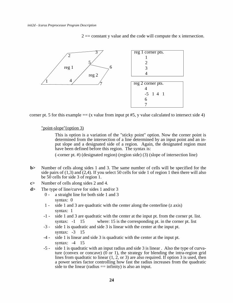
2 == constant y value and the code will compute the x intersection.
"point-slope"(option 3)This is option is a variation of the "sticky point" option. Now the corner point isdetermined from the intersection of a line determined by an input point and an in-put slope and a designated side of a region. Again, the designated region musthave been defined before this region. The syntax is:(-corner pt. #) (designated region) (region side) (3) (slope of intersection line)
b> Number of cells along sides 1 and 3. The same number of cells will be specified for theside pairs of (1,3) and (2,4). If you select 50 cells for side 1 of region 1 then there will alsobe 50 cells for side 3 of region 1.
c> Number of cells along sides 2 and 4.d> The type of line/curve for sides 1 and/or 3
0 - a straight line for both side 1 and 3syntax: 0
1 - side 1 and 3 are quadratic with the center along the centerline (z axis)syntax: 1
-1 - side 1 and 3 are quadratic with the center at the input pt. from the corner pt. list.syntax: -1 15 where: 15 is the corresponding pt. in the corner pt. list
-3 - side 1 is quadratic and side 3 is linear with the center at the input pt.syntax: -3 15
-4 - side 1 is linear and side 3 is quadratic with the center at the input pt.syntax: -4 15
-5 - side 1 is quadratic with an input radius and side 3 is linear . Also the type of curva-ture (convex or concave) (0 or 1), the strategy for blending the intra-region gridlines from quadratic to linear (1, 2, or 3) are also required. If option 3 is used, thena power series factor controlling how fast the radius increases from the quadraticside to the linear (radius == infinity) is also an input.
reg 1
reg 21
23
4
56
7
reg 1 corner pts.1234
reg 2 corner pts.4-5 1 4 167
corner pt. 5 for this example == (x value from input pt #5, y value calculated to intersect side 4)
24

init2d - Icarus Preprocessor Program Description
syntax: -5 0 1-5 1 2-5 1 3 1.1
-6 - side 3 is quadratic and 1 is linear with the same input format as option -5.
e> Cell Spacing along sides 1 and 3. Spacing of the cells either can be uniform or the cellscan be clustered to one or both ends.
0 - Uniform spacing1 - Manually assign cell spacing via cell weights, 30 per line following this input line2 - Cluster cells toward the lower number of side; that is, towards side 2.For this op-
tion, two additional inputs are required. The first specifies the size variation fromcell to cell using a simple geometry ratio. For a value of 1.03, a 3% cell size varia-tion will be obtained. The second sets the ratio of maximum to minimum cell size.This limits the smallest cell size.syntax: 2 1.05 100.
3 - Cluster cells toward the higher number side or side 4. The inputs are the same asfor option 2.syntax: 3 1.03 200.
4 - Cluster cells towards both sides (2 and 4). The inputs are the same as for option 2.syntax:4 1.05 150.
f> Cell Spacing along sides 2 and 4. Spacing of the cells either can be uniform or the cellscan be clustered to one or both ends. The syntax is the same as for the proceeding option.
g> Boundary conditions for sides 1 through 4 are specified. Each side must have a specificboundary condition type.1 Line of symmetry (rz axis)2 Line of symmetry (xy axis)3 Constant freestream bc from the inlet table+/-3x Freestream bc using an inlet table.5 Solid surface+/-5x Solid surface with sources from an inlet table7 Connection to another region or multiple regions+/-7x Region connection with sources from an inlet table9 Porous wall (porosity specified in the variable, value, on surface info. #45)
or mixed boundary type (solid surface and region connectivity)+/-9x Porous wall or mixed boundary with sources from an inlet table11 Outflow (non-reentrant, vacuum pump of infinite speed)
(note type 11 cannot be used for a region connection)12 Same as type 9. Computes net flux on type 9 if a type 12 bc is adjacent.
(note: typically have type 9 BC as the ‘upstream’ boundary and 12 as the ‘downstream’ boundary) - MUST have a 9-12 pair
13 zero-gradient outflow (Neumann-like). The code computed the Maxwellian dist.from the upstream cell and samples from this distribution to obtain the particles toinject back into the domain to yield a zero-gradient boundary
25

init2d - Icarus Preprocessor Program Description
Boundary types +/-3x, +/-5x, +/-7x,and +/-9x require a table entry be specified for ‘x’.This specifies the table number to refer to in the inlet file. The boundary conditiontype can be + or -; positive number indicates that coordinate specified in the inletfile is either x or z, a negative boundary condition indicates that the coordinate iseither y or r. Examples are: -51, and 32.
h> Number of surface specification input lines (#46). Required for boundary conditions 5, 5x,9 and 9x.
i> Surface specification input variables on each line are:1 - Region side number 2 &3 - Define the starting and stopping cell number for this specification.
note: this feature can input piecewise property variations along a surface--cells are numbered as:
side 1-- cell 1 adjoins side 1-2 intersectionside 2 -- cell 1 adjoins side 1-2 intersectionside 3 -- cell 1 adjoins side 2-3 intersectionside 4 -- cell 1 adjoins side 1-4 intersection
4 - The number of evenly spaced surface elements per cell. This option can be used togreatly increase the accuracy of the solution of the Poisson Electro-statics equationby the Boundary Element Method without the tremendous cpu time penalty in-curred by simply increasing the number of cells.
5 - Amount of specular reflection in Maxwell Model (0.0 for fully diffuse) (Chapter 1)6 - Temperature of the surface (K).7 - Material number associated with material number defined in the surf_bc file.
(input 0 if no surface chemistry). A number without a surf_bc input can be usedto ‘mark’ a particular surface for postprocessing with surface2d.
8 - Porosity for boundary type 9 and 9x (value of 1.0 for freeflow, 0.0 for no flow)(input 0.0 for boundary conditions other than type 9)
Note: to define a linear variation of temperature and/or porosity:1-use a line entry for each ‘end point’ of the linear range (cell number domain)2-set the region side number (first entry) to negative....3-both temperature and porosity will be varied linearly between the endpoints
j> Region connectivity table. In most cases, multiple regions will need to be connected to de-fine the specific geometry.
There are four rows in the region connectivity table, one for each side. The entries are:1 - side number2 - the number of connecting regions to this side. For example, if a side is a solid sur-
face there are no connecting regions and the entry is 0.If 2nd value is non-zero, then there must be ((input 2)*2) numbers to follow, one pair for
each connecting region.3 - input pair which specify the connected region side number and region number in
clockwise fashion for that side (see example below).
26

init2d - Icarus Preprocessor Program Description
The diagram below shows two examples of region connectivity based on the clockwiserule.
In example 1, regions 2 and 3 are connected to side 1 of region 1. Applying the clockwiserule results in a region numbering sequence 3 and 2 on side 1 of region 1. Similarly, in ex-ample 2, regions 2 and 3 are connected to side 3 of region 1. In this case the connectivity or-der will be regions 2 and 3 to side 3 of region 1.
Example 1 - region 1 connectivity input for side 1:12 3 3 3 2Example 2 - region 1 connectivity input for side 3:32 1 2 1 3
Boundary type 9 allows for multiple boundary type specification; for example side 4 of re-gion 1 is connected to another region and is partly a solid surface:
boundary type for side 4 of region 1 == 9 surface specification (input #45) is required for side 4-- the porosity variable is used forthe connecting side (1.0 for freeflow between the regions)example: 4 1 50 0.0 300. 0 0.95
(the surface is defined to be at 300K and a porosity of 95% is used ONLY for the portionwhich connects to region 2. You do not have to have the region cell boundaries lineup onthe region1-region 2 interface. The code logic will determine the correct particle trajec-
tory. Also, the cell range of 1-50 simply needs to be inclusive of the actual number ofcells.)
(1)
(2) (3)
EXAMPLE 1 EXAMPLE 2
(1)
(2) (3)Region 1: side 1
Order will start withRegion 3 and end with Region 2
Region 1: side 3
Order will start withRegion2 and endwith Region 3
1
2
34
1
23
4
12
3
4
1
2
3
4
12
3
41
2
3
4
(1)
(2)
1
2
3
4 1
2
3
4
27

init2d - Icarus Preprocessor Program Description
Example region connectivity for side 4 of region 1:4 2 2 2 2 -1
Note: a pseudo-region, -1, is used to indicate where the solid surface is. Alternating re-gions and pseudo-regions can be used to build complex geometries (see samples section).
28

init2d - Icarus Preprocessor Program Description
alpha
.0
.0
.0
.0
.0
.0
3.5 Species File Description (spec)
Example file:
•Lines beginning with ’*’ are comments and are not used.
•The first data entry MUST be the number of species to input.
•The second data entry MUST be the number of degrees of freedom which describes themost complex molecule.
3 - translational modes (one for each direction)4 - rotational + translational modes (for diatomic molecules)5 - vibrational + rotational + translational modes
The default model is for a single vibrational temperature; quantized models are also available
**************************************** species data file ****************************************6 number of species*3 internal structure of most complex molecule:* 3-monatomic, 4-rotation, 5-rotat. + vibrat.*1 # of chemical reactions*** NOTE: Fe- electron mass increased by 1000 ---- use ONLY for steady state simulations!!!!**-------------------------------------------------------------------------------------------------------------------* ID* Mwt Mol. mass Diam. #Rot.Deg. Rot.Rel. # Vib. Deg. Vib. Rel. Vib.Temp. specie wt. charge omega tref * (kg) (m) Freedom Coll. # Freedom Coll. # (K)*---------------------------------------------------------------------------------------------------------------------------------* D2 4.02 0.668e-26 0.2701e-9 0.0 0.0 0.0 0.0 0.0 1.0 0.0 0.67 300. 1D 2.01 0.334e-26 0.2211e-09 0.0 0.0 0.0 0.0 0.0 1.0 0.0 0.67 300. 1D2+ 4.02 0.668e-26 0.2701e-9 0.0 0.0 0.0 0.0 0.0 1.0 +1.0 0.67 300. 1D+ 2.01 0.334e-26 0.2211e-09 0.0 0.0 0.0 0.0 0.0 1.0 +1.0 0.67 300. 1Fe- 5.45e-4 0.9049e-27 6.941e-8 0.0 5. 0. 0.0 0.0 1.0 -1.0 1.0 300. 1e- 5.45e-4 0.9049e-30 6.941e-8 0.0 5. 0. 0.0 0.0 1.0 -1.0 1.0 300. 1*END*
29

init2d - Icarus Preprocessor Program Description
•The third data entry MUST be the number of chemical reactions to be read in. Thechemistry filename will be chem (default) or user provided by the ’chemistry file’ inputoption.
•The next data section describes each species. The order of the species in this file isvery important; this order is assumed throughout the calculation.
Each species requires two lines of input. line 1: species chemical symbol (used in postprocessing files, 6 characters long)line 2: description of the species for transport and interactions:
molecular weight, molecular mass (kg), molecular diameter (m), # of rotational degrees of freedom, rotational relaxation collision number, # of vibrational degrees of freedom, vibrational relaxation collision #,
vibrational temperature, species weight (described below), charge number, omega (collision model - viscosity), reference T (K) for omega and alpha, alpha (VSS collision model - diffusivity) .
If either not modelling or have no information for rotational/vibrational interactions,enter 0.0.
Species weighting is a strategy used to increase statistics on species that exist in lowconcentrations. Only two different specie weights are allowed: 1.0 and a number < 1.0.In the example, you will see that either 1.0 or 0.02 are used for species weight. A spe-cies weight less than 1 multiplies the cell ratio of the # of real molecules per simulatedone. For example, consider a mixture of 2 species: one with a mole fraction of 0.99 andthe other 0.01. If the weights were equal to 1.0 for both species and there were 100computational particles in the cell, 99 would be species 1 and 1 particles would be spe-cies 2. Thus, if there were only 20 particles in the cell, on the average, the 20 particleswould all be species type 1! If the species weight was 0.02 for species 2, then on the av-erage, the cell would have 14 particles of species 1 and 6 of species 2. Species weightmust be a number between 0.0 and 1.0!
By default, interspecies omega and alpha are simply the arithmetic average of the indi-vidual species values. If information is available, these defaults can be overridden inthe following optional input section.
•This is the optional input section:
alpha i j rThis is used to override the default arithmetic average for an alpha for species i andj with value r.
omega i j rThis is used to override the default arithmetic average for an omega for species iand j with value r.
tref i j rThis is used to override the default arithmetic average for a tref for species i and jwith value r.
30

init2d - Icarus Preprocessor Program Description
vibration model i Flag to use a different vibrational model (temperature dependent relaxation) suchas the Miliken & White model. The model will be user supplied; an example canbe found in the eos.f code module. (default value = 0)
rotational model iFlag to use a different rotational model (temperature dependent) such as the Milik-en & White model. The model will be user supplied; an example can be found inthe eos.f code module. (default value = 0)
• The last input line MUST be END.
31
init2d - Icarus Preprocessor Program Description
3.6 Inlet File Description (inlet)
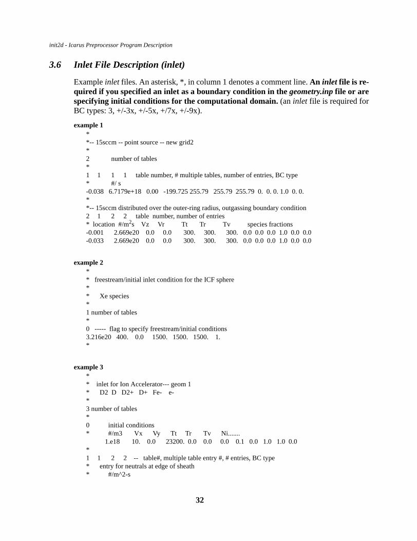
Example inlet files. An asterisk, *, in column 1 denotes a comment line. An inlet file is re-quired if you specified an inlet as a boundary condition in the geometry.inp file or arespecifying initial conditions for the computational domain. (an inlet file is required forBC types: 3, +/-3x, +/-5x, +/7x, +/-9x).
example 1**-- 15sccm -- point source -- new grid2*2 number of tables*1 1 1 1 table number, # multiple tables, number of entries, BC type* #/ s-0.038 6.7179e+18 0.00 -199.725 255.79 255.79 255.79 0. 0. 0. 1.0 0. 0.**-- 15sccm distributed over the outer-ring radius, outgassing boundary condition2 1 2 2 table number, number of entries* location #/m2s Vz Vr Tt Tr Tv species fractions -0.001 2.669e20 0.0 0.0 300. 300. 300. 0.0 0.0 0.0 1.0 0.0 0.0-0.033 2.669e20 0.0 0.0 300. 300. 300. 0.0 0.0 0.0 1.0 0.0 0.0
example 2** freestream/initial inlet condition for the ICF sphere** Xe species*1 number of tables*0 ----- flag to specify freestream/initial conditions3.216e20 400. 0.0 1500. 1500. 1500. 1.*
example 3** inlet for Ion Accelerator--- geom 1* D2 D D2+ D+ Fe- e-*3 number of tables*0 initial conditions* #/m3 Vx Vy Tt Tr Tv Ni....... 1.e18 10. 0.0 23200. 0.0 0.0 0.0 0.1 0.0 1.0 1.0 0.0*1 1 2 2 -- table#, multiple table entry #, # entries, BC type* entry for neutrals at edge of sheath* #/m^2-s
32

init2d - Icarus Preprocessor Program Description
0.000 1.0e24 9.3e5 0.00 23206. 23206. 23206. 0.0 0.1 0.0 1.0 0.0 0.0 0.00056 1.0e24 9.3e5 0.00 23206. 23206. 23206. 0.0 0.1 0.0 1.0 0.0 0.0*1 2 2 2* 0.000 1.0e24 2.9e4 0.00 1. 1. 1. 0.0 0.0 0.0 0.0 1.0 0.0 0.00056 1.0e24 2.9e4 0.00 1. 1. 1. 0.0 0.0 0.0 0.0 1.0 0.0
*File Description
line 1:Number of tables to be read (number of separate inlets).
for each table:first line:Table number, # in multiple table, number of entries, table type
table number: sequential number only used for ordering the inputif == 0, this is a flag to indicate initial domain and freestream conditionsfor a boundary condition type 3 (volume source). There are no other in-puts on the first line for a table number 0 (see above example 2).
multiple tables: Multiple inlet boundary conditions can be defined for a given sur-face--for example, a two stream, two specie source where the fluxes andtemperatures were different for each species. Simply enter a table entryfor stream source and index the 2nd number in the first line (multiple ta-ble option): the multiple table option would be ‘1’ for the first streamsource, ‘2’ for the second, etc (see above example 3). Note that bothmultiple tables are numbered ’1’. The ‘# in multiple table’ must be se-quential and incremental: 1,2,3.etc.
number of entries: the number of entries for that inlet table. The entries between theinput locations are linearly interpolated; to input a inlet profile, simplyuse more entries for the table.
table (boundary condition) types:1 -- point source, #/s (1 sccm = 4.48e17 #/s)2 -- surface flux, #/m2-s (note--a unit depth of 1m is assumed in cartesian (XY) coordinates)3 -- volume source, #/m3
next lines:single input line for each table entry- inlet location, BC type specifies coordinate (m)
The inlet location can be either x or y (z or r in axisymmetric systems). A sin-gle coordinate is used since the inlet boundary conditions must be along a re-gion boundary; the init2d code determines the second coordinate to machine
33

init2d - Icarus Preprocessor Program Description
accuracy. If the BC type code specified in geometry.inp is negative (i.e. -31,-52, -93, etc.) then the inlet location coordinate is assumed to be either y or r. Ifthe BC type code is positive, the inlet coordinate is either x or z.
- flow rate (units depend on the BC type)- boundary types: 3x, 5x, 7x, or 9x, each can have either a 1, or 2, or 3 type
boundary.- for a point source (+/-5x), 1sccm = 4.48e17 #/s- multiple point sources can exist along a boundary- For BC 2 and 3, linear interpolation is used between input values; profiles are
modelled as a series of line segments.- BC type +/-3x is generally used for a ‘line’ inflow boundary condition- BC type +/-5x if for a point source (small inlet nozzle - code 1) or for an out-
gassing surface (code 2).- BC type +/-9x is for the special case where a region has both a surface and re-
gion connection on the same side or for a porous connection between re-gions.
- Vx or Vz average inlet velocity vector (m/s)The input velocities are the average velocities; the translational temperature isused to obtain the velocity distribution which is sampled for the inlet particlevelocity.- use standard sonic flow relationships (see Chapter 10) to obtain both orifice
velocities and exit temperatures (V* and T*)- make sure that the velocity vectors are into the computational domain!
- Vy or Vr average inlet velocity vector (m/s)
- Translational Temperature (K for non-electrons, eV for electrons)NOTE: for table number = 0 (initial/freestream conditions), the translational temp.
is in K for all species (init2d will convert to eV if electron species are present)
- Rotational Temperature (K)
- Vibrational Temperature (K)
- species mole fractions in same order as geometry.inp and spec file
34

init2d - Icarus Preprocessor Program Description
3.7 Surface Boundary Condition File (surfbc)
The surface boundary condition file contains a separate table for each type of materialspecified in the geometry.inp file. An asterisk, *, in column 1 denotes a comment line. This filecontrols both surface chemistry, translating/rotating walls, applied potentials, and other boundaryinputs. They are differentiated by the line 1 input: the boundary condition type variable.
Surface reaction probability can be defined with a simple sticking coefficient or it can be afunction of site coverage. The surface coverage model is simple: sites are either occupied or va-cant. Thus, only one type of surface species can be defined. Ion energy sputtering yield can alsobe described for a surface reaction using the expression A(Ea
ion - Eath)b as defined by Gray et al.
(J. Vac. Sci. Technol. A, vol. 12, pp. 354-364, 1994). In the event that a product is not formed dur-ing an ion surface reaction an alternate reaction product can be specified to insure ion neutraliza-tion.
For Example: CF3+ + SiO2-Coverage(surface site) -------> SiF4 + CO2 or CF3
Example surfbc input files:
example 1** this file contain surface chemistry information for the Poisson test - H2 chemistry* D2 D2+ D D+ e-* 1 2 3 4 5** variable order for each reaction:* (Rx type) (Species-i) (Species-r1) (Species-r2) (create prob-1)* (create prob 2) (degree of specular reflect) (Rx prob)** For type 8: type icode voltbc eps1 eps2 0. 0. 0.*3 number of material table types** material 2 voltage=100V2 1 1.4e168. 1. 100. 0. 0.0 0. 0. 0.0** material 3, mirror bc (Enormal = 0), specular3 1 1.4e168. 2. 0. 0. 0.0 0. 0. 0.0** material 4 voltage=10V4 1 1.4e168. 1. 10. 0. 0.0 0. 0. 0.0
example 2
35

init2d - Icarus Preprocessor Program Description
** this file contain surface chemistry information for tube2 - H2 chemistry* D2 D2+ D D+ e-* 1 2 3 4 5** variable order for each reaction:* (Rx type) (Species-i) (Species-r1) (Species-r2) (create prob-1)* (create prob 2) (degree of specular reflect) (Rx prob)** For type 8: type icode voltbc eps1 eps2 0. 0. 0.*10 number of material table types** material 1 screen plate -- voltage=0KV, ions neutralize, e stick1 5 1.4e161. 2. 1. 0. 1.0 0. 0. 1.0 D2+ --> D21. 3. 1. 0. 0.5 0.0 0.0 0.1 D --> D21. 4. 3. 5. 1.0 1.5 0. 1.0 D+ --> D + 1.5e-1. 5. 5. 0. 0.0 0. 0. 1.0 e- --> stick8. 1. 0. 0.0 0.0 0. 0. 0.0** material 2 accel. plate -- voltage=-100kV, ions neutralize, e stick2 5 1.4e161. 2. 1. 0. 1.0 0. 0. 1.01. 3. 1. 0. 0.5 0.0 0.0 0.1 H ---> H21. 4. 3. 5. 1.0 1.5 0. 1.01. 5. 5. 0. 0.0 0. 0. 1.08. 1. -100000.0 0.0 0.0 0. 0. 0.0** material 3, source -- 5 voltage bc, all sticks- electrons reflect3 5 1.4e161. 2. 1. 0. 1.0 0. 0. 1.0 D2+ --> D21. 3. 1. 0. 0.5 0.0 0.0 0.1 D --> D21. 4. 3. 5. 1.0 1.5 0. 1.0 D+ --> D + 1.5e-1. 5. 5. 0. 1.0 0. 1. 1.0 e- --> reflect8. 1. 5. 0.0 0.0 0. 0. 0.0** material 4, dielectric (Neumann for now)4 4 1.4e161. 3. 1. 0. 0.5 0.0 0.0 0.1 H ---> H21. 4. 3. 5. 1.0 1.5 0. 1.01. 5. 5. 0. 0.0 0. 0. 1.0****8. 3. 0. 1. 9.0 0. 0. 0.08. 2. 0. 0. .0 0. 0. 0.0** material 5, target -- time dependent voltage bc* secondary electron emission5 6 1.4e161. 1. 1. 0. 0.0 0. 0. 1.01. 2. 2. 0. 0.0 0. 0. 1.01. 3. 3. 0. 0.0 0. 0. 1.0
36

init2d - Icarus Preprocessor Program Description
1. 4. 3. 5. 1.0 1.5 0. 1.01. 5. 5. 0. 0.0 0. 0. 1.08. 5. 00.0 0.5 300.0 -100000. 0. 0.0** material 6, mirror bc (Enormal = 0), specular6 1 1.4e168. 2. 0. 0. 0.0 0. 0. 0.0** material 7 accel. plate back side- ions neutralize, e stick7 4 1.4e161. 2. 1. 0. 1.0 0. 0. 1.01. 3. 1. 0. 0.5 0.0 0.0 0.1 H ---> H21. 4. 3. 5. 1.0 1.5 0. 1.01. 5. 5. 0. 0.0 0. 0. 1.0** material 8 backside of target -- voltage=0, ions neutralize, e stick8 5 1.4e161. 2. 1. 0. 1.0 0. 0. 1.01. 3. 1. 0. 0.5 0.0 0.0 0.1 H ---> H21. 4. 3. 5. 1.0 1.5 0. 1.01. 5. 5. 0. 0.0 0. 0. 1.08. 6. 00.0 0.5 120.0 0. 0. 0.0* material 9 --- internal structures 0V- slow ions -- expansion region9. 5. 1.75e191. 4. 3. 0. 1. 0. 0.0 0.5 H+ --> H1. 3. 1. 0. 0.5 0.0 0.0 0.1 H ---> H21. 2. 1. 0. 1. 0. 0. 0.5 H2+ --> H21. 5. 5. 0. 0.0 0. 0. 1.08. 2. 0.0 0.0 0.0 0. 0. 0.0* material 10 --- external walls 0V- slow ions -- expansion10. 5. 1.75e191. 4. 3. 0. 1. 0. 0.0 0.5 H+ --> H1. 3. 1. 0. 0.5 0.0 0.0 0.1 H ---> H21. 2. 1. 0. 1. 0. 0. 0.5 H2+ --> H21. 5. 5. 0. 0.0 0. 0. 1.08. 1. 0.0 0.0 0.0 0. 0. 0.0
File Description
Line 1: Number of material tables
For each table:first line:Table number, number of entry sets per table, site density(#/m2).
Table number: identifier used in the input file for the surface definition. The order isnot important
number of entries: the number of data sets (not necessary lines) per table. A data setcan be either one or two lines.
site density: only used for surface dependent chemistry (coverage model). if not, useany input value
37

init2d - Icarus Preprocessor Program Description
data sets (either one or two lines per material)•required input line(A) required for all BC types (8 real entries)boundary condition types +/-1 thru +/-8): Types 1 thru 6 specify surface chemistrywhere a positive reaction type indicates that the reaction rate is not temperature depen-dent and no ion energy dependent yield information is required. A negative reactiontype indicates an extra line is read in to allow for surface temperature dependence andfor ion energy dependent yield parameters. Type 7 is a translating/rotating boundary.Type 8 indicates boundary conditions to be used in the Poisson electrostatic field solv-er. Note that all boundaries defining the fields must be specified as surface elementsonce and only once; that is, if a zero width structure is in the domain, do not have sur-face elements with electrostatic boundary conditions on both sides.
entry1: BC type:+/-1 Simple model (no coverage dependence)+/-2 Absorption reaction - takes open surface site.+/-3 Etch reaction - vacates occupied surface site.+/-4 Requires an open site but leaves the surface unchanged.+/-5 not used at this time+/-6 not used at this time+/-7 translating or rotating boundary8 boundary condition used for electrostatics (Poisson field solver)
For BC types 1 through 6 (surface chemistry):entry 2: reacting species number (corresponding to spec and geometry.inp files)entry 3: reaction product species #1entry 4: reaction product species #2 (specify 0. if only one reaction product)entry 5: creation probability species #1entry 6: creation probability species #2entry 7: degree of surface specular reflection (0.0 for diffuse)entry 8: Surface reaction probability (A)
For BC type +/-7 (translating or rotating surface):entry 1: +7 translating surface (cartesian coordinate system)
-7 rotating surface (axisymmetric coordinate system)entry 2: u-velocity (x-direction), m/s (for translating surface)entry 3: v-velocity (y-direction), m/s (for translating surface)entry 4: rotational speed , rev/s (MUST be axisymmetric coordinate system)entry 5: 0.0entry 6: 0.0entry 7: 0.0
38

init2d - Icarus Preprocessor Program Description
entry 8: 0.0
For BC type 8 (electrostatic BC):entry 2: icode to specify the type of BC for the Poisson electrostatic solver:
0 = surface NOT included in electrostatics calcs.1 = applied potential, volts (direchlet)2 = surface normal field is zero (neumann)3 = dielectric material (not currently implemented)4 = time varying surface potential (AC) superimposed on DC potential
V(t) = VDC + Vo sin (2 π ω t)5 = a current based bc.....requires resistance drop to a constant voltage6 = ’backside’ boundary for icode=5 .... allows a bc without a surface
charge element7 = periodic bc -- electrically equivalent to icode =28 = surface element with constant potential -- value from runtime input9 = flag for an icode=1 element internal to domain....code reverses the
surface unit normal and changes it to an icode=1 element<0 = floating conductor (computes surface charge and redistribution
on a constant voltage surface) (not verified)entry 3: if (icode.eq.1) applied potential, volt,
else set to 0.0entry 4: if (icode.eq.4) then its the magnitude of the AC component (volts)
if (icode.eq.5) then its the backward time averaging factor=1 for implicit (no time averaging)
else set to 0.0entry 5: if (icode.eq.4) then its the rf frequency (Hz)
if (icode.eq.5) then its the resistance to a constant potentialelse set to 0.0
entry 6: if (icode.eq.5) then its the constant potential via the resistance, voltelse set to 0.0
entry 7: 0.0entry 8: 0.0
For BC types -1 through -6 (surface chemistry):entry 2: reacting species number (corresponding to spec and geometry.inp files)entry 3: reaction product species #1entry 4: reaction product species #2 (specify 0. if only one reaction product)entry 5: creation probability species #1entry 6: creation probability species #2
39

init2d - Icarus Preprocessor Program Description
entry 7: degree of surface specular reflection (0.0 for diffuse)entry 8: Surface reaction probability (A)Additional line(B) for surface reactions with temperature dependence or ion ener-
gy dependence (7 entries on second line)
entry 1: B - surf. reaction temperature dependence (for Arrhenius fit K = ATBe(Ea/T))
entry 2: Ea (joules) - surf. reaction activation energyentry 3: A - energy dep. etch yield in the form of A(Ea
ion - Eath)b
entry 4: a - energy dep. etch yield parameterentry 5: b - energy dep. etch yield parameterentry 6: Eth (joules) - energy dep. etch yield threshold energyentry 7: alternate reaction product, species #1
The creation probability contains reaction stoichiometry information; for Cl etch to createSiCl2 the creation probability is 0.5 because it will only form once for two Cl’s that hit thesurface. (Cl --> 1/2 SiCl2..... the 1/2 is the creation probability per incident particle)
examples:
•Cl recombination to Cl2 can be described as either an overall reaction with a wall recombina-tion coefficient of 0.1 for Cl --> 1/2 Cl2 (fully diffuse reflected product):
1. 1. 4. 0. 0.5 0. 0. 0.1
Or, Cl recombination can be described as a two step process dependent on surface coverage:
Cl + Si(s) -> SiCl(s) (reaction type 1)
Cl + SiCl(s) -> SiCl2(g) + Si(s) (reaction type 2)
2. 1. 0. 0. 0.0 0. 0. 1.03. 1. 4. 0. 1.0 0. 0. 0.05
An example of temperature dependent etching rate is given for C2F6 etch of SiO2* OMEGA C2F6 plasma simulations with 10 rnxs, 11 species* C2F6 F2 CF3 F F+ CF3- SiF4 CF2 CF2+ CF CF+ O2 CO2 CF3+* 1 2 3 4 5 6 7 8 9 10 11 12 13 14 1 number of material table types** material 1 (oxide wafer SiO2 etch)1 9 1.75e192. 4. 0. 0. 0.0 0.0 0.0 0.22. 10. 0. 0. 0.0 0.0 0.0 0.33
40

init2d - Icarus Preprocessor Program Description
2. 8. 0. 0. 0.0 0.0 0.0 0.332. 3. 0. 0. 0.0 0.0 0.0 0.33-3. 14. 7. 13. 1.0 1.0 0.0 1.0
0. 0. .053 .5 1.0 6.4e-19 3.-3. 5. 7. 12. 1.0 1.0 0.0 1.0
0. 0. .053 .5 1.0 6.4e-19 4.0-3. 9. 7. 13. 1.0 1.0 0.0 1.0
0. 0. .053 .5 1.0 6.4e-19 8.-3. 11. 7. 13. 1.0 1.0 0.0 1.0
0. 0. .053 .5 1.0 6.4e-19 10.1. 6. 6. 0. 1.0 0.0 1.0 1.0
Example surf_bc file:** this file contain surface chemistry information for the* UH - GEOM1 Problem Cl2 chemistry * Cl, Cl+ , Cl-, Cl2, Cl2+, SiCl2* 1 2 3 4 5 6*2 number of material table types etch of Si --> SiCl2 ** material 1 (wafer), wafer 1. 7. 1.75e19 table number, number of entries(reactions), site density(#/m2)* Following input defines surface reactions on material type #1*First two reactions are Cl recombination to Cl2 with surface coverage * dependence (see explanation below)2. 1. 0. 0. 0.0 0. 0. 1.03. 1. 4. 0. 1.0 0. 0. 0.05* Next reaction is Cl- reflecting at wall fully specular due to sheath.1. 3. 3. 0. 1.0 0.0 1. 1.0* Cl+ and Cl2+ ion etching (doesn’t include values for energy dependent * etch yield)3. 2. 6.0 0. 1.0 0. 0. 1.01. 5. 6.0 0. 1.0 0. 0. 1.0** material 2, upper head 2. 4. 1.75e191. 1. 4. 0. 0.5 0. 0. 1.01. 2. 1. 0. 1.0 0.0 0. 1.01. 3. 3. 0. 1. 0.0 1. 1.0 1. 5. 4. 0. 1.0 0.0 0. 1.0
41

init2d - Icarus Preprocessor Program Description
3.8 Cross Section File (cross_section)
This file is used to specify a constant cross-section for a particle-particle interaction in-stead of the default VHS model. For cross-sections not specified in this file, the VHS model willbe used. It can also be used to input a chemical reaction rate or interaction event in a JANEV 9-order polynomial fit format. An asterisk, *, in column 1 denotes a comment line.
Example cross_section files:
example 1* cross section input file - overwrite the VHS based values* file for charged particles and neutral *9 02 1100.e-202 4100.e-202 6100.e-203 1100.e-203 4100.e-203 6100.e-205 1100.e-205 4100.e-205 6100.e-20
example 2* cross section input file - overwrite the VHS based values** first line == # constant inputs, # reaction fits* note: ICARUS in SI....so sigma in m**2.....*0 1** charge exchange rx. for : p + H(1s) ---> H(1s) + p* fit# type Emin sigma(Emin) sigmax multiplier 1 6 0.1 7.e-15 7.e-15 1.e-4 (in cm**2)* fits for #1-3.27412379e1 -8.9164565e-2 -3.01699076e-02 9.2054824e-3 2.40026656e-3-1.92712231e-3 3.65475034e-4 -2.78886646e-5 7.422296363e-7
42
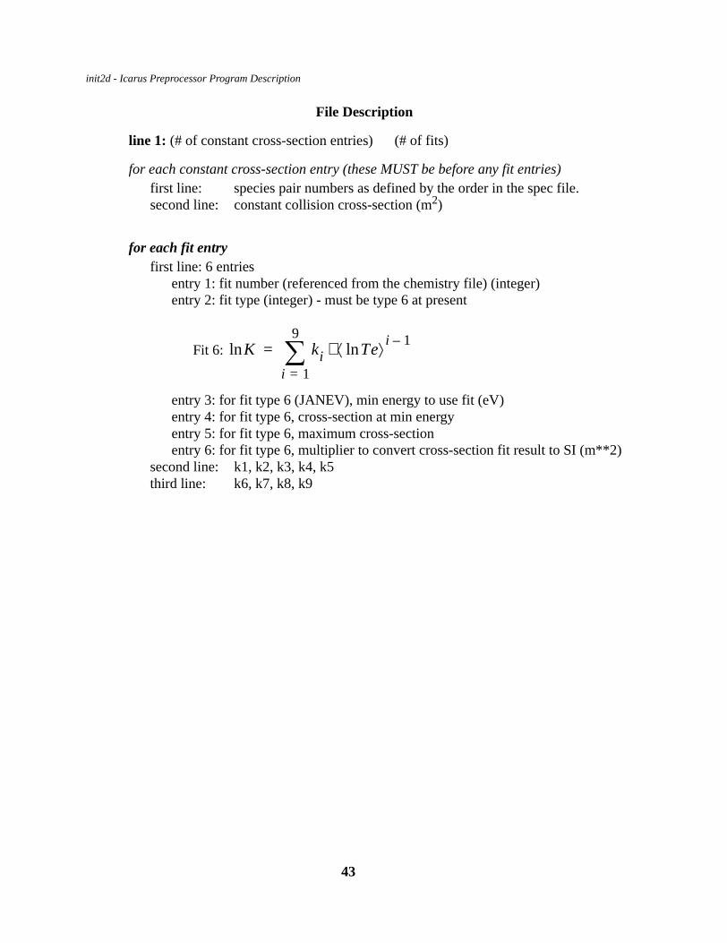
init2d - Icarus Preprocessor Program Description
File Description
line 1: (# of constant cross-section entries) (# of fits)
for each constant cross-section entry (these MUST be before any fit entries)first line: species pair numbers as defined by the order in the spec file.second line: constant collision cross-section (m2)
for each fit entry first line: 6 entries
entry 1: fit number (referenced from the chemistry file) (integer)entry 2: fit type (integer) - must be type 6 at present
Fit 6:
entry 3: for fit type 6 (JANEV), min energy to use fit (eV)entry 4: for fit type 6, cross-section at min energyentry 5: for fit type 6, maximum cross-sectionentry 6: for fit type 6, multiplier to convert cross-section fit result to SI (m**2)
second line: k1, k2, k3, k4, k5third line: k6, k7, k8, k9
Kln ki Teln⟨ ⟩ i 1–⋅i 1=
9
∑=
43

init2d - Icarus Preprocessor Program Description
3.9 Gas Phase Chemistry File (chem or chem.asc)The number of gas phase reactions is defined in the geometry.inp file and must match the
chemistry input file. Two formats are allowed for the chemistry input: the standard Icarus chemis-try format as defined for the file (chem) or the standard Chemkin format (chem.asc). The defaultis the DSMC chemistry format; set the number of chemical reactions in the geometry.inp file to itsnegative for the Chemkin input option. A Icarus formatted file is also generated with theChemkin option (output file == chem). The Chemkin file, chem.asc, is generated from user inputby the Chemkin Interpreter (not included in this software package). An asterisk, *, in column 1denotes a comment line.Example file:
*Hydrogen Chemistry Input File: 2/4/1999* 2/4/99: Electron Species included* Excitation energies corrected* Note multiplier on rate is 10-6, units for rate m^3.* Source of cross sections from "Elementary Processes in Hydrogen-Helium Plasmas", by,* R.K. Janev, et al, Springer Series on Atoms and Plasmas, * Springer-Verlag (Berlin, Heidelberg, New York) 1987.* web address for data: www.iaea.org/programmes/amdis/ala/aladdin_7.txt** updated for different product grouping - new init2d chemistry reader*----------------------------------------------------------------------------* This input file contains the data characterizing the chemical reactions.* If input # reactions = 0, there is no chemistry, and this file is not read.* input lines are free format* the reaction equation is an input line (a25)*----------------------------------------------------------------------------*** NOTE: line 0 character string illustrating the reaction* line 1 defines rx. stoichiometry* line 2 for type 0, -1, & -2 MUST have 5 real numbers* line 2 for type -3 MUST have 2 integers and 1 real number* line 3 for type -3 MUST have 6 real numbers**** first number on line 1 defines reaction type:** 0 -- standard Arrhenius collisional chemistry k = A T^B exp(-Ea/kT)* second line variables:* 1 -- number of internal degrees of freedom* 2 -- Ea* 3 -- A* 4 -- B* 5 -- heat of rx (+ for exothermic) - joules** -1 -- Charge Exchange reaction with fixed rate* second line variables:* 1 -- 0 - constant, else == cross-secton input table #* 2 -- sigma CE (m^2)** -2 -- Charge Exchange reaction using model from Rapp & Frances(1962)* sigma = ( k1 - k2*alog(vr) )**2* second line variables:* 1 -- k1 for elastic collision* 2 -- k2 for elastic collision* 3 -- k1 for charge exchange
44

init2d - Icarus Preprocessor Program Description
* 4 -- k2 for change exchange** -3 -- Electron Impact reactions* second line variables:* 1 -- equation type (if <0, T in K instead of eV)* 2 -- number of products (1 or 2)* 3 -- heat of formation (Frank-Candom)- joules* third line variables:* 1 - 6 are fit coefficients ** ** Hydrogen --- # 1 --------** D2 D2+ D D+ e-* 1 2 3 4 5** !!!!Mulitplier on Rates is 10-6 since rates in m^3 (cross sections m^2)!!!!!* **REACTION TYPENOTE1. e + D2(GS) => e + D(1s) + D(1s)Dissociation-3 5 1 1 2 5 3 3 6 0 0.96e-19 10.00 32 1 1.26 3.25e-12 3.82e-9 1.e-6 -2.858072836568e+01 1.038543976082e+01 -5.383825026583e+00 1.950636494405e+00 -5.393666392407e-01 1.006916814453e-01 -1.160758573972e-02 7.411623859122e-04 -2.001369618807e-05 *2. e + D2(GS) => e + D(1s) + D(2s)Dissociation-3 5 2 1 2 5 3 3 6 0 0.96e-19 14.933 1 2.51 7.88e-12 6.92e-9 1.e-6 -3.454175591367e+01 1.412655911280e+01 -6.004466156761e+00 1.589476697488e+00 -2.775796909649e-01 3.152736888124e-02 -2.229578042005e-03 8.890114963166e-05 -1.523912962346e-06*3. e + D2(GS) => e + D(2p) + D(2s)Dissociation-3 5 1 1 2 5 3 3 6 0 0.0 23.0 34 1 5.01 6.48e-12 1.31e-9 1.e-6 -4.794288960529e+01 2.629649351119e+01 -1.151117702256e+01 2.991954880790e+00 -4.949305181578e-01 5.236320848415e-02 -3.433774290547e-03 1.272097387363e-04 -2.036079507592e-06*4. e + D(1s) => e + (e + D+)Ionization-3 5 3 1 2 5 4 5 6 0 0.0 13.6 25 1 2.0 7.22e-12 3.11e-8 1.e-6 -3.271396786375e+01 1.353655609057e+01 -5.739328757388e+00 1.563154982022e+00 -2.877056004391e-01 3.482559773737e-02 -2.631976175590e-03 1.119543953861e-04 -2.039149852002e-06 *5. e + D(2s) => e + (e + D+)Ionization-3 5 3 1 2 5 4 5 6 0 0.0 3.4 26 1 0.398 8.87e-12 1.71e-7 1.e-6 -1.973476726029e+01 3.992702671457e+00 -1.773436308973e+00 5.331949621358e-01 -1.181042453190e-01 1.763136575032e-02 -1.616005335321e-03 8.093908992682e-05 -1.686664454913e-06*6. e + D2 => e + (e + D2+(v))Ionization-3 5 1 1 2 5 2 5 6 0 0.0 15.435 1 2.0 2.34e-12 5.18e-8 1.e-6 -3.568640293666e+01 1.733468989961e+01 -7.767469363538e+00 2.211579405415e+00 -4.169840174384e-01 5.088289820867e-02 -3.832737518325e-03 1.612863120371e-04 -2.893391904431e-06
45

init2d - Icarus Preprocessor Program Description
*7. e + D2 => e + (e + D(1s) + D+ )Dissociative Ionization -3 5 1 1 3 5 5 3 4 6 0 0.0 18.036 1 3.98 3.74e-12 2.89e-9 1.e-6 -3.834597006782e+01 1.426322356722e+01 -5.826468569506e+00 1.727940947913e+00 -3.598120866343e-01 4.822199350494e-02 -3.909402993006e-03 1.738776657690e-04 -3.252844486351e-06*8. e + D2+(v) => e + (e + D+ + D+ )Dissociative Ionization-3 5 2 1 3 5 5 4 4 6 0 0.0 14.7 37 1 3.16 5.23e-12 9.06e-9 1.e-6 -3.746192301092e+01 1.559355031108e+01 -6.693238367093e+00 1.981700292134e+00 -4.044820889297e-01 5.352391623039e-02 -4.317451841436e-03 1.918499873454e-04 -3.591779705419e-06*9. e + D2+(v) => e + D+ + D(1s)Dissociative Ionization-3 5 2 1 2 5 4 3 6 0 0.0 2.4 38 1 0.2 1.23e-12 1.15e-7 1.e-6 -1.781416067709e+01 2.277799785711e+00 -1.266868411626e+00 4.296170447419e-01 -9.609908013189e-02 1.387958040699e-02 -1.231349039470e-03 6.042383126281e-05 -1.247521040900e-06*10. e + D2+(v) => e + D+ + D(n=2) Dissociative Ionization-3 5 2 1 2 5 4 3 6 0 0.0 14.0 39 1 2.0 5.03e-12 1.77e-7 1.e-6 -3.178647420e+01 1.573560727511e+01 -6.992177456733e+00 1.852216261706e+00 -3.130312806531e-01 3.383704123189e-02 -2.265770525273e-03 8.565603779673e-05 -1.398131377085e-06*11. e + D2+(v) => D(1s) + D*(n)Dissociative Recombination-3 5 2 0 2 3 3 6 0 0.0 0.00 40 1 0.1 2.23e-7 2.23e-7 1.e-6 -1.670435653561e+01 -6.035644995682e-01 -1.942745783445e-08 -2.005952284492e-07 2.962996104431e-08 2.134293274971e-08 -6.353973401838e-09 6.152557460831e-10 -2.025361858319e-11 *12. D+ + D(1s) => D(1s) + D+ Charge Exchange-1 4 3 1 1 3 4 1.0 7.e-15 0. 0. 0.*13. e + D(1s) => e + D(2p)Excitation-5 5 3 1 1 5 3 6 0 0.0 10.2 34 1 1.26 4.78e-12 3.18e-9 1.e-6 -2.814949375869e+01 1.009828023274e+01 -4.771961915818e+00 1.467805963618e+00 -2.979799374553e-01 3.861631407174e-02 -3.051685780771e-03 1.335472720988e-04 -2.476088392502e-06*14. e + D(1s) => e + D(2s) Excitation-5 5 3 1 1 5 3 6 0 0.0 10.2 34 1 1.26 3.54e-12 3.22e-9 1.e-6 -2.833259375256e+01 9.587356325603e+00 -4.833579851041e+00 1.415863373520e+00 -2.537887918825e-01 2.800713977946e-02 -1.871408172571e-03 6.986668318407e-05 -1.123758504195e-06*15. e + D(2s) => e + D(2p) Excitation-5 5 3 1 1 5 3 6 0 0.0 0.00001934 34 1 0.1 1.18e-12 1.18e-9 1.e-6 -1.219616012805e+01 -3.859057071006e-01 -6.509976401685e-03 4.981099209058e-04 -4.184102479407e-05 3.054358926267e-06 -1.328567638366e-07 8.974535105058e-10 1.010269574757e-10*16. e + D2(v=0) => e + D2(v=1) Vibrational Excitation
46

init2d - Icarus Preprocessor Program Description
-5 5 1 1 1 5 1 6 0 0.0 0.5 34 1 0.158 5.83e-12 2.6e-9 1.e-6 -2.017212494454e+01 9.563952280637e-01 -6.931474225637e-01 1.673671529631e-01 -3.228762898855e-02 5.838603222226e-03 -8.580542691302e-04 7.456311623168e-05 -2.666978300757e-06*17. e + D2(v=0) => e + D2(v=2) Vibrational Excitation-5 5 1 1 1 5 1 6 0 0.0 1.0 34 1 0.398 5.93e-12 7.07e-10 1.e-6-2.265507686305e+01 2.239943592222e+00 -1.099426577160e+00 2.339027647223e-01 -2.528511103871e-02 6.851302489620e-04 1.253426182224e-04 -1.253475051672e-05 3.545892878015e-07*18. e + D2(GS) => e + D2(EX ST 1)Excitation-5 5 1 1 1 5 1 6 0 0.0 11.37 34 1 2.0 9.88e-12 1.47e-8 1.e-6 -3.081902926338e+01 1.038866780735e+01 -4.259768348687e+00 1.181228673120e+00 -2.277513907465e-01 2.900576728856e-02 -2.287591474628e-03 1.004346442778e-04 -1.869930069131e-06*19. e + D2(GS) => e + D2(EX ST 2) Excitation-5 5 1 1 1 5 1 6 0 0.0 11.7 34 1 2.0 3.59e-12 1.39e-8 1.e-6 -3.348199796300e+01 1.371702271009e+01 -5.922607900694e+00 1.709719148860e+00 -3.505232830275e-01 4.834376067841e-02 -4.131406425550e-03 1.948388368131e-04 -3.854278715563e-06*20. e + D2(GS) => e + D2(EX ST 3) Excitation-5 5 1 1 1 5 1 6 0 0.0 12.2 34 1 3.16 5.27e-12 2.23e-9 1.e-6-3.646589741675e+01 1.430361969329e+01 -6.074430521073e+00 1.677305768580e+00 -3.128705597349e-01 3.805424730473e-02 -2.860085821803e-03 1.199641410078e-04 -2.142231851104e-06
File Description:This is the standard Icarus chemistry input file. Formats for different types of reactions
(elastic gas, charge exchange, and electron impact) are slightly different however, all reactionsfollow the same basic input structure. Reaction format: A + B --> (C + E) + (D + F).
First line: Character string (or comment line)
Second line:entry 1: reaction type (integer)
0 elastic gas rxn - kinetic treatment-1 charge exchange rxn (fixed cross-section or Janev fit)-2 charge exchange rxn using Rapp and Francis relationship-3 electron impact rxn-4 elastic gas rxn - continuum treatment (for trace-trace chemistry)-5 electron excitation reactions (used for electron energy balance)
entry 2: species number for reactant Aentry 3: species number for reactant B
47

init2d - Icarus Preprocessor Program Description
entry 4: stoichiometric coefficient for the first product groupentry 5: stoichiometric coefficient for the second product groupentries 6-9 are the species number of the product species depending of existence
C D orC E D F orC D F orC E D
Third line: (depends on reaction type)Reaction type 0 or -4: Elastic gas reaction
Arrhenius collisional chemistry reaction rate expression: k = A TB exp(-Ea/kT)T in K. Requires 5 real numbers:
entry 1 -- number of internal degrees of freedomentry 2 -- Eaentry 3 -- Aentry 4 -- Bentry 5 -- heat of rx (+ for exothermic) - joules
Reaction type -1: Charge exchange with cross-section, σRequires 2 real numbers:
entry 1 -- cross-section table #; set == 0.0 for constant σMUST have a cross-section input table
entry 2 -- σ (m2) - constant
Reaction type -2: Charge exchange using model from Rapp & Frances(1962) sigma = ( k1 - k2*alog(vr) )**2
Requires 4 real numbers:entry 1 -- k1 for elastic collisionentry 2 -- k2 for elastic collisionentry 3 -- k1 for charge exchangeentry 4 -- k2 for charge exchange
For example, this format was used by Kilgore, Wu and Graves (J. Vac. Sci. Tech-nol. B 12(1)) for an Ar plasma for MKS units on velocity. The following parametervalues are given:
7.746x10⁻¹⁰ 4.493x10⁻¹¹ 1.288x10⁻⁹ 7.436x10⁻¹¹
48

init2d - Icarus Preprocessor Program Description
Reaction type -3 or -6: Electron Impact reactionsRequires 2 integer numbers and 2 real numbers
entry 1 -- equation fit types (if <0, Te in K instead of eV)Fit 1: K = k1 * (Te**k2) * exp(-k3 / Te)Fit 2: K = k1 * (Te**k2) * exp(-k3 * Te)Fit 3: K = k1 * ((k2 / Te) ** k3)Fit 4: K = k1 * (Te**k2) * exp((k3 / Te) + (k4/Te**2) + (k5/Te**3) +
(k6/Te**4))Fit 5: K = k1 + (Te*k2) + (k3*Te**2) + (k4*Te**3) + (k5*Te**4) +
(k6*Te**5)
Fit 6: (Janev format)
entry 2 -- 0.0 - not usedentry 3 -- heat of formation (e.g., Franck-Condon)- joulesentry 4 -- energy loss per electron reaction - ev
If | fit # | = 1, 2, or 3input line:
k1, k2, k3if | fit # | = 4 or 5
input line:k1, k2, k3, k4, k5, k6
If | fit # | = 6 (Janev format)first line:
entry 1: reaction # (integer)entry 2: 1.0 (form of fit - only option at present)entry 3: min energy to use fit (eV)entry 4: cross-section at min energyentry 5: maximun cross-sectionentry 6: multiplier to convert cross-section fit result to SI (m**2)
second line: k1, k2, k3, k4, k5
third line:k6, k7, k8, k9
Kln ki Teln⟨ ⟩ i 1–⋅i 1=
9
∑=
49

init2d - Icarus Preprocessor Program Description
Two other example chem files follow:
Example 1: A 23 equation set of elastic gas reactions for air chemistry with 5 species: O2,N2, O, N, and NO. Species 1 == O2, 2==N2, etc.
*O2 + N --> 2O + N 0 1 4 2 1 3 3 4 1. 8.197E-19 5.993E-12 -1. -8.197E-19 *O2 + NO --> 2O + NO 0 1 5 2 1 3 3 5 1. 8.197E-19 5.993E-12 -1. -8.197E-19 *O2 + N2 --> 2O + N2 0 1 2 2 1 3 3 2 1.5 8.197E-19 1.198E-11 -1. -8.197E-19 *2O2 --> 2O + O2 0 1 1 2 1 3 3 1 1.5 8.197E-19 5.393E-11 -1. -8.197E-19 *O2 + O --> 3O 0 1 3 2 1 3 3 3 1. 8.197E-19 1.498E-10 -1. -8.197E-19 *N2 + O --> 2N + O 0 2 3 2 1 4 4 3 0.5 1.561E-18 3.187E-13 -0.5 -1.561E-18 *N2 + O2--> 2N + O2 0 2 1 2 1 4 4 1 0.5 1.561E-18 3.187E-13 -0.5 -1.561E-18 *N2 + NO --> 2N + NO 0 2 5 2 1 4 4 5 0.5 1.561E-18 3.187E-13 -0.5 -1.561E-18 *2N2 --> 2N + N2 0 2 2 2 1 4 4 2 1. 1.561E-18 7.968E-13 -0.5 -1.561E-18 *N2 +N --> 3N 0 2 4 2 1 4 4 4 1. 1.561E-18 6.9E-8 -1.5 -1.561E-18 *NO + N2 --> N+O+N2 0 5 2 2 1 4 3 2 1. 1.043E-18 6.59E-10 -1.5 -1.043E-18 *
50

init2d - Icarus Preprocessor Program Description
NO + O2 --> N+O+O2 0 5 1 2 1 4 3 1 1. 1.043E-18 6.59E-10 -1.5 -1.043E-18 * NO + NO --> N+O+NO 0 5 5 2 1 4 3 5 1. 1.043E-18 1.318E-8 -1.5 -1.043E-18 *NO + O --> N + O + O0 5 3 2 1 4 3 3 1. 1.043E-18 1.318E-8 -1.5 -1.043E-18 *NO + N --> 2N + O 0 5 4 2 1 4 3 4 1. 1.043E-18 1.318E-8 -1.5 -1.043E-18 *NO + O --> O2 + N 0 5 3 1 1 1 4 0. 2.719E-19 5.279E-21 1. -2.719E-19 *N2 + O --> NO + N 0 2 3 1 1 5 4 0. 5.175E-19 1.120E-16 0. -5.175E-19 *O2 + N --> NO + O 0 1 4 1 1 5 3 0. 4.968E-20 1.598E-18 0.5 2.719E-19*
NO + N --> N2 + O 0 5 4 1 1 2 3 0. 0. 2.49E-17 0. 5.175E-19*O+O + M1 --> O2 + M1 (note M1 denotes a third body partner -- the entry of -1 indicates the table in-dex0 3 3 1 0 1 0 -10. 0. 8.297E-45 -0.5 8.197E-19*N+N + M2 --> N2 + M2 *0 4 4 1 0 2 0 -20. 0. 3.0051E-44 -0.5 1.561E-18*N + N + N --> N2 + N 0 4 4 1 0 2 0 -30. 0. 6.3962E-40 -1.5 1.5637E-18 *N+O + M3 --> NO + M3 0 4 3 1 0 5 0 -4 0. 0. 2.7846E-40 -1.5 1.043E-18
51

init2d - Icarus Preprocessor Program Description
Example 2: Chlorine plasma with charge exchange and electron impact chemistry
** Chlorine chemistry example -- 11 reaction set** Cl, Cl+, Cl-, Cl2, Cl2+, SiCl2, e-* 1 2 3 4 5 6 7** Cl+ + Cl -> Cl + Cl+ (charge exchange)-1 2 1 1 1 1 2 0.75 120.e-20 0. 0. 0.*Cl2+ + Cl2 -> Cl2 + Cl2+ (charge exchange)-1 5 4 1 1 4 5 0.75 120.e-20 0. 0. 0.**Cl- + Cl -> Cl + Cl- (charge exchange)*-1 3 1 1 1 1 3* 0.90 120.e-20 0. 0. 0.**Cl+ + Cl- -> Cl + Cl (recombination)-4 2 3 1 1 1 1 0.0 0.0 5.e-14 0.0 1.5e-18*Cl2+ + Cl- -> 2Cl + Cl (recombination)-4 5 3 2 1 1 1 0.0 0.0 5.e-14 0.0 1.26e-18** Cl2 attachment to Cl + Cl- (electron impact)-3 7 4 1 1 1 3 2 2 5.78e-19 0.0 Franck-Condon 2.21e-16 0.485 -0.174 0.0 0.0 0.0* Cl- detachment to Cl (electron impact)-3 7 3 2 1 7 7 1 1 1 0.0 3.61 2.94e-14 0.680 3.7994 0.0 0.0 0.0* Cl2 dissociation to 2Cl (electron impact)-3 7 4 2 1 1 7 1 1 2 0.96e-19 3.12 3.99e-14 0.115 4.43 0.0 0.0 0.0* Cl2 ionization to Cl2+ (electron impact)-3 7 4 2 1 7 7 5 1 1 0.0 11.47 2.13e-14 0.771 11.7 0.0 0.0 0.0* Cl ionization to Cl+ (electron impact)
52

init2d - Icarus Preprocessor Program Description
-3 7 1 2 1 7 7 2 1 1 0.0 12.99 2.96e-14 0.554 13.1 0.0 0.0 0.0* Cl2+ attachment to 2Cl (electron impact)-3 7 5 1 1 1 1 3 2 1.84e-18 0.0 9.0e-13 0.0258526 0.61 0.0 0.0 0.0** electron exicitation reactions -- type -5* from E. Meeks 0-D code -- MKS --- T in Kelvin* Cl2 -- vibrational ex.-5 7 4 1 1 7 4 -1 1 0.0 0.07Chem.asc (Chemkin file) use: 2.5141E-08 -1.4443E+00 1.6650E+04 0.0 0.0 0.0 Cl2 -- electronic ex.-5 7 4 1 1 7 4 -1 1 0.0 9.25 6.3477E-12 -5.3987E-01 1.3920E+05 0.0 0.0 0.0 Cl -- 4s -5 7 1 1 1 7 1 -1 1 0.0 9.55 1.2363E-11 -6.1356E-01 1.3297E+05 0.0 0.0 0.0 Cl -- 5s -5 7 1 1 1 7 1 -1 1 0.0 10.85 3.4801E-12 -6.6984E-01 1.4944E+05 0.0 0.0 0.0 Cl -- 6s -5 7 1 1 1 7 1 -1 1 0.0 12.55 1.9354E-12 -7.3244E-01 1.7005E+05 0.0 0.0 0.0 Cl -- 3d -5 7 1 1 1 7 1 -1 1 0.0 11.65 9.4444E-11 -7.3093E-01 1.5413E+05 0.0 0.0 0.0 Cl -- 4d -5 7 1 1 1 7 1 -1 1 0.0 12.45 7.6428E-11 -7.7209E-01 1.6452E+05 0.0 0.0 0.0 Cl -- 5d -5 7 1 1 1 7 1 -1 1 0.0 12.75 4.7440E-11 -7.8620E-01 1.6810E+05 0.0 0.0 0.0 Cl -- 4p -5 7 1 1 1 7 1 -1 1 0.0 10.85 1.2295E-10 -8.0133E-01 1.4248E+05 0.0 0.0 0.0 Cl -- 5p -5 7 1 1 1 7 1 -1 1 0.0 12.15 4.9579E-11 -8.4151E-01 1.5872E+05 0.0 0.0 0.0
53

init2d - Icarus Preprocessor Program Description
Chem.asc (Chemkin file) use:
The chem.asc file is generated when the Chemkin Interpreter is run. Below is a brief de-scription of the chem.inp file used by the Chemkin Interpreter to generate chem.asc, a more de-tailed description, taken from reference 4 is given in Appendix B. When Init2d is run with achem.asc file it generates a standard Icarus chem file (named chem_ck), this allows the user tochange the chemistry without having to rerun the Chemkin Interpreter.
Some constraints exist in using Chemkin files for Icarus. 1.) Stoichiometric coefficient of reactants in the chem.inp file must be 1. This will not
show up as an error when running the Chemkin Interpreter but is not allowed inIcarus. Init2d will flag this as an error.
2.) Degree’s of freedom for all reactions is assumed to be 1.3.) Reaction type -2 (from Icarus chem file) is not allowed when using the Chemkin input
file. To add these types of reactions to an existing mechanism that is already in thechemkin format, run Init2d using the chem.asc file and a chem_ck file will be gener-ated. The chem_ck file can be edited and renamed chem to include reaction types -2and then Init2d must be rerun.
4.) Troe parameters or pressure dependent reaction rates are not allowed in Icarus.
There are four sections to a chemkin input file that are indicated by the following keywords: Elements, Species, Thermo, and Reactions. All sections are followed with the wordEnd. Comments are any and all characters following as exclamation mark. Details of the formatused for the Chemkin Interpreter are found in Appendix B.
Elements contains declaration of all elements contained in any gas phase species.
Species contains all species used in the gas phase mechanism. The format of these speciesmust be the same as the format used in the Icarus spec file, Init2d will compare thelist of species declared in the spec file and compare it to the species found inchem.inp file. All species in the spec file must be declared in the chemkin inputfile.
Thermo contains all thermodynamic data for species. This information is not used inIcarus but is required to run the chemkin interpreter. If information in not containedin the input file it must be present in the thermodynamic data base file therm.dat sup-plied with chemkin. Details of this information can be found in Appendix C.
Reactions contains descriptions of the gas phase reactions, parameters for Arrhenius rateexpression (k = ATβexp (-Ea/T)), and excitation energies. All reactions, except chargeexchange reactions, require the first line of information to include:
54

init2d - Icarus Preprocessor Program Description
reaction description in ASCII textA βEaCharge exchange reactions (type -1 from chem) with constant cross section require
slightly different input information:reaction description in ASCII textprobability σ(m2) 0.0Auxiliary information is placed on subsequent lines such as excitation energy, temper-
ature dependence (electron temperature dependence for electron impact reactions),etc. The most likely auxiliary key words to be used for Icarus simulations are:
EXCI/ 0.07/ (Excitation energy for the reaction is 0.07 eV) TDEP/E/ (Specifies that Arrhenius temperature dependence) DUP (Indicates a duplicate reaction exists in the mechanism, this is typically
used for excitation reactions.)
Example 1: Chemkin input file (chem.inp) for a Chlorine plasma chemistry mechanismwith Boltzman EEDF to determine rates. This is the same file that was used in Aurora (SNL 0DPlasma code), although charge exchange reactions have been added.
ELEMENTS E CL ENDSPECIES E CL+ CL2+ CL- CL CL2 ENDTHERMO ALL300 1000 5000E 71091E 1 0 0 0G 300.000 10000.000 1000.00 0 1 0.25002515E+01 0.00000000E+00 0.00000000E+00 0.00000000E+00 0.00000000E+00 2-0.74597845E+03-0.11736856E+02 0.25002515E+01 0.00000000E+00 0.00000000E+00 3 0.00000000E+00 0.00000000E+00-0.74597839E+03-0.11736856E+02 4CL 112293CL 1 0 0 0G 300.000 4000.000 1000.00 0 1 0.29181864E+01-0.35438285E-03 0.12474453E-06-0.20015567E-10 0.11864538E-14 2 0.13713931E+05 0.32732935E+01 0.23711388E+01 0.96051756E-03 0.23850609E-06 3-0.20040531E-08 0.11036082E-11 0.13841132E+05 0.60661221E+01 4CL* 112293CL 1 0 0 0G 300.000 4000.000 1000.00 0 1 0.29181864E+01-0.35438285E-03 0.12474453E-06-0.20015567E-10 0.11864538E-14 2 0.13713931E+05 0.32732935E+01 0.23711388E+01 0.96051756E-03 0.23850609E-06 3-0.20040531E-08 0.11036082E-11 0.13841132E+05 0.60661221E+01 4CL+ 112293CL 1E -1 0 0G 300.000 4000.000 1000.00 0 1 0.30344462E+01-0.48197978E-03 0.15346743E-06-0.12604539E-10-0.32295198E-15 2 0.16550063E+06 0.29831080E+01 0.25186882E+01 0.99940156E-03 0.96029623E-07 3-0.22788400E-08 0.13577272E-11 0.16558978E+06 0.55090742E+01 4CL- 112293CL 1E 1 0 0G 300.000 4000.000 1000.00 0 1 0.25002515E+01 0.00000000E+00 0.00000000E+00 0.00000000E+00 0.00000000E+00 2-0.28878172E+05 0.41883583E+01 0.25002515E+01 0.00000000E+00 0.00000000E+00 3 0.00000000E+00 0.00000000E+00-0.28878168E+05 0.41883578E+01 4CL2 112293CL 2 0 0 0G 300.000 4000.000 1000.00 0 1 0.41252842E+01 0.68196526E-03-0.40838054E-06 0.11656516E-09-0.11435189E-13 2-0.12794418E+04 0.30671713E+01 0.33467176E+01 0.34548617E-02-0.36136810E-05 3 0.13227441E-08-0.66440849E-14-0.11213928E+04 0.68718143E+01 4CL2+ 112293CL 2E -1 0 0G 300.000 4000.000 1000.00 0 1 0.41252842E+01 0.68196526E-03-0.40838054E-06 0.11656516E-09-0.11435189E-13 2
55

init2d - Icarus Preprocessor Program Description
0.13183581E+06 0.30671713E+01 0.33467176E+01 0.34548617E-02-0.36136810E-05 3 0.13227441E-08-0.66440849E-14 0.13199384E+06 0.68718143E+01 4ENDREACTIONS KELVIN MOLECULES! reaction rates from Boltzmann w/ LFA, 50%Cl/50%Cl2, .1% electrons! reaction A(molecules-cm-s) b Ea(K) E + CL2 => E + CL2 4.2051E-03 -1.3229E+00 1.0572E+04 TDEP/E/ !vibrational ex EXCI/ 0.07/ DUP E + CL2 => CL- + CL 1.1061E-10 7.3354E-02 2.2957E+03 TDEP/E/ !dissociative a E + CL2 => 2CL + E 4.3770E-10 3.6734E-01 6.1276E+04 TDEP/E/ !dissociation E + CL2 => E + CL2 4.0373E-04 -7.9572E-01 2.3857E+05 TDEP/E/ !electronic exc EXCI/ 9.25/ DUP E + CL2 => CL2+ + 2E 1.7109E-01 -1.0671E+00 3.4343E+05 TDEP/E/ !ionization E + CL- => CL + 2E 3.3777E-07 -7.1844E-02 8.6257E+04 TDEP/E/ !detachment E + CL => E + CL* 2.2229E-01 -1.3555E+00 2.4567E+05 TDEP/E/ !4s excitation E + CL => E + CL 2.2229E-01 -1.3555E+00 2.4567E+05 TDEP/E/ !4s excitation EXCI/ 9.55/ DUP E + CL => E + CL 1.3323E+01 -1.8428E+00 3.0150E+05 TDEP/E/ !5s excitation EXCI/10.85/ DUP E + CL => E + CL 2.1643E+03 -2.3564E+00 3.6940E+05 TDEP/E/ !6s excitation EXCI/12.55/ DUP E + CL => E + CL 1.4842E+05 -2.4057E+00 3.3453E+05 TDEP/E/ !3d excitation EXCI/11.65/ DUP E + CL => E + CL 1.1564E+06 -2.6237E+00 3.6620E+05 TDEP/E/ !4d excitation EXCI/12.45/ DUP E + CL => E + CL 2.6560E+06 -2.7462E+00 3.7772E+05 TDEP/E/ !5d excitation EXCI/12.75/ DUP E + CL => E + CL 6.8249E+04 -2.4070E+00 3.0212E+05 TDEP/E/ !4p excitation EXCI/10.85/
56
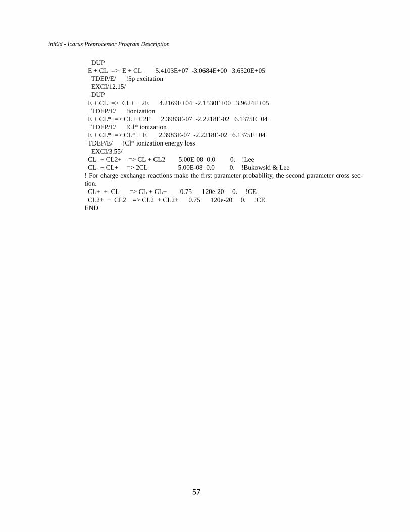
init2d - Icarus Preprocessor Program Description
DUP E + CL => E + CL 5.4103E+07 -3.0684E+00 3.6520E+05 TDEP/E/ !5p excitation EXCI/12.15/ DUP E + CL => CL+ + 2E 4.2169E+04 -2.1530E+00 3.9624E+05 TDEP/E/ !ionization E + CL* => CL+ + 2E 2.3983E-07 -2.2218E-02 6.1375E+04 TDEP/E/ !Cl* ionization E + CL* => CL* + E 2.3983E-07 -2.2218E-02 6.1375E+04 TDEP/E/ !Cl* ionization energy loss EXCI/3.55/ CL- + CL2+ => CL + CL2 5.00E-08 0.0 0. !Lee CL- + CL+ => 2CL 5.00E-08 0.0 0. !Bukowski & Lee! For charge exchange reactions make the first parameter probability, the second parameter cross sec-tion. CL+ + CL => CL + CL+ 0.75 120e-20 0. !CE CL2+ + CL2 => CL2 + CL2+ 0.75 120e-20 0. !CE END
57

init2d - Icarus Preprocessor Program Description
3.10 Diagnostic Messages
The init2d code checks for several types of problem areas:
1- length of program arrays-see section 9.2 for adjusting the parameters in init2d.h
2- region side connectivity-the code will check the region side connectivity consistency. An error will occur if the region connectivity section is not consistent between two regions
3- files-the code will provide output to indicate when an input file is opened and closed to facilitate debugging
4- the final screen output from the init2d code contains problem size definitioninformation. This can be used to determine parameters for the param.h file for Icarus,post2d and decomp2d. (section 9.2)
5- Surface boundary conditions are checked to determine if there are sufficient input foreach type
6- Warnings are provided when using some of the options. For example, a porous boundary with a porosity of 0.0 (solid wall).
7- The grid is checked in an indirect manner since linear quadrilateral elements are used to determine interpolant and derivative shape functions. Shape errors can occur when
the region sides do not conform to the naming convention of init2d.
58

59
4.0 decomp2d - Decomposition Code Description
Goal: Decomposes the problem for parallel computing environment.
Usage:decomp2d param1 param2
param1 and param2 can be entered either on the command line, as shown, orin response to interactive questions.
param1: number of processors to decompose the input file, datap, intoparam2: decomposition strategy (1 for sequential and 2 for block)
(recommend 1 for massively parallel and 2 for few processors)
Input files:datap: geometry and boundary definition file from init2d
Output files:dsmc.in2: decomposed data file -- specific to # of processorsdsmc.node: link list file to associate cell information with a processor.
used by restart2d
Notes:
decomp2d does NOT need to be used if a single processor simulation is being done. Theoutput file from init2d, datap, can be used directly by icarus.
We use decomposition strategy 1 for a tightly coupled computer such as a nCUBE and 2for other systems: network of workstations, quad-PCs, SGI Power Challenge, IBM parallel sys-tems at LLNL or Maui. .
5.0 icarus - Code and Command File (dsmc.in) Description
Goals: Performs particle move & collisions (DSMC with optional electro-static fields) andgathers statics.
Usage: icarus < dsmc.in
dsmc.in is a command line redirected input file
Input Files: dsmc.in2(MP), datap(1P) (file names defined in dsmc.in file)dsmc.restart (for restart calculation)dsmc.plasma, dsmc.power (for icp plasma application)
Output Files: Output filenames are defined in the dsmc.intypical names are: cell.*, surf.* , wafer.*, chem.*, plasma.*, and particle.*.* denotes the overall time step when file was written (i.e. cell.2000)
File Descriptions:cell.* Contains macroscopic quantities of pressure, temperature, density, spe-
cies concentrations and velocities. Local Cell Knudsen number, CFLnumber and λ are also contained in this file. An external program, post2d,is used to determine macroscopic properties, determine the type of outputvariables, and generate a Tecplot formatted plot file.
surface.* Contains surface element information such as incident flux by species,reflected flux (etchant), surface coverage, surface pressure, shear stressand heat flux. The external program, surface2d, is used to generate a Tec-plot formatted plot file.
wafer.* Contains wafer element information of angular and energy distributionfunctions by species. The external program, waferxy2d, is used to gener-ate a Tecplot formatted plot file.
chem.* Contains statistics of the number of times each chemical reaction oc-curred per cell. The external program, post2d, is used to generate a Tec-plot formatted plot of the chemical reaction statistics.
plasma.* Contains electron number density and temperature for each cell. The ex-ternal program, post2d, is used to generate a Tecplot formatted plot file ofthe plasma fields, potential, and local charge density.
particle.* Contains information on ALL computational particles: position, velocity,species, and kinetic energy
dsmc.log Contains log information of an Icarus run such as number of time steps,number of particles, number of collisions, number of surface collisions,etc.
dsmc.pump Contains pump and pressure information when using the pressure feed-back loop. Output includes old pressure at control point, new pump speedand current pressure at control point.This file can be used to provide pres-sure histories at various points during the simulation.
60

icarus - Code and Command File (dsmc.in) Description
5.1 icarus Command List Summary
This is a complete list of valid DSMC commands found in the dsmc.in file, their defaults,and the “type” of parameters that should be used (i=integer, r=real, c=character string). Thetype (integer, real, character string) of the parameters is important since the input parser expectscertain kinds of values. All of the input commands take one or more parameters. The keyword foreach command must begin in the left most column and all characters in the command must be inlower-case. Parameters can be separated by arbitrary numbers of spaces and/or tabs.
Note: a ‘*’ or ‘#’ as the first character denotes a comment linetypical entries are shown---they may or may not be the defaults
i/o fileslog file dsmc.log (c)id string character string (c)cell file cell (c)surface file surface (c)wafer file wafer (c)movie file movie (c)chemistry file chem (c)plasma file plasma (c)particle file particle (c)pump file pump (c)icp file icp.out (c)directory name (c)
problem initializationread definition 1.0 dsmc.def (rc)read restart 1.0 1.0 dsmc.def dsmc.restart (rrcc)read xrestart 1.0 1.0 dsmc.def dsmc.restart (rrcc)read efield dsmc_em (c)read plasma dsmc_plasma (c)read power dsmc_power dsmc_plasma (cc)load particles 1.0 (r)loadn cutoff 0 (i)loadv cutoff 0 (i)
61

icarus - Code and Command File (dsmc.in) Description
output controlunformatted 0 (i)output screen 100 (i)output cells 0 (i)output surface 0 (i)output wafer 0 (i)output movie 0 0.1 (i)output chemistry 0 (i)output plasma 0 (i)output particles 0 (i)output fx 0 (i)ion energy 30.0 (r)neutral energy 1.0 (r)species energy 3 20.0 (ir)output special 50 dsmc.nbari (ic)
collision/chemistry controlcollision flag 1 (i)chemistry flag 0 (i)exchange flag 0 (i)collision limit 5 (i)secondary electron 0 (i)coverage 0 (i)electron chemistry 0 (i)ereact limit 0 (i)coulomb 0 (i)no ionchem 99999 (i)ion collide 0 (i)
particle injection/gas-surfacesurface model 1 (i)thermal accom 1.0 (r)BC model 0 (i)BC ramp 0.0 (r)inletbc multiplier 1.0 (r)surface dist 1.0 (r)voltage bc 0.0 (r)quasi-neutral bc 1 (i)target model 1 (i)
62
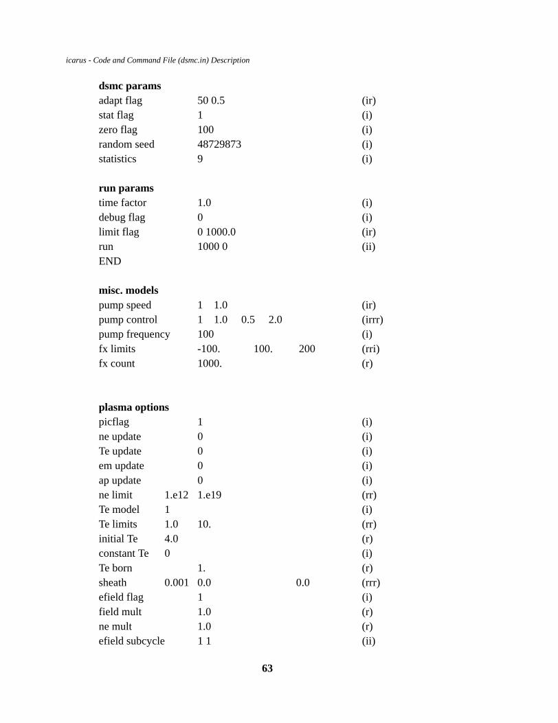
icarus - Code and Command File (dsmc.in) Description
dsmc paramsadapt flag 50 0.5 (ir)stat flag 1 (i)zero flag 100 (i)random seed 48729873 (i)statistics 9 (i)
run paramstime factor 1.0 (i)debug flag 0 (i)limit flag 0 1000.0 (ir)run 1000 0 (ii)END
misc. modelspump speed 1 1.0 (ir)pump control 1 1.0 0.5 2.0 (irrr)pump frequency 100 (i)fx limits -100. 100. 200 (rri)fx count 1000. (r)
plasma optionspicflag 1 (i)ne update 0 (i)Te update 0 (i)em update 0 (i)ap update 0 (i)ne limit 1.e12 1.e19 (rr)Te model 1 (i)Te limits 1.0 10. (rr)initial Te 4.0 (r)constant Te 0 (i)Te born 1. (r)sheath 0.001 0.0 0.0 (rrr)efield flag 1 (i)field mult 1.0 (r)ne mult 1.0 (r)efield subcycle 1 1 (ii)
63

icarus - Code and Command File (dsmc.in) Description
e subcycle 1 (i)ion subcycle 1 (i)surface charge 0 (i)volume charge 0 (i)power model 0 (i)moving average 10 (i)charge averaging 1.0 (r)ne average 0 (i)ion source 0 (i)charge regions 4 5 0 (iii)ambipolar regions 4 5 1 (iii)charge void 4 5 0 (iii)charge density 1.e20 (r)icp flag 0 (i)ln(lambda) 10. (r)charge distance 1.e-6 (r)ion power 0.0 1.e-5 1.e-5 1 500. 1.e23 10. (rrrirrr)
64

icarus - Code and Command File (dsmc.in) Description
5.2 Icarus Command Descriptions
# commentsblank lines are ignored. Everything on a line after last parameter is ignored. Lines startingwith a ‘*’ or ‘#’ are comments and are echoed into the log file.
-------------------------------i/o files------------------------------------
log fileAll info from this point on will dump into this file. Any previous file is closed. New filename can exist, will be overwritten. Anything in input file before the first “log file” com-mand will not be echoed into a log file.default = none
id stringfollowing character string will be printed at top of output filesdefault = none
cell filename of cell file to dump to; timestep # is appended to name. the file can exist--will beoverwritten. default = cell
surface filename of surface file to dump to; timestep # is appended to name. the file can exist--will beoverwrittendefault = surf
wafer filename of wafer file to dump to; timestep # is appended to name. the file can exist--will beoverwrittendefault = wafer
movie filename of movie file to dump unsteady particle information to; timestep # is appended toname. the file can exist--will be overwrittendefault = moviechemistry filename of file to write chemical reaction statistics to; timestep # is appended to name. thefile can exist--will be overwrittendefault = chem
65

icarus - Code and Command File (dsmc.in) Description
plasma filename of the file to write plasma properties (electric field vectors, plasma potential, and lo-cal charge density) to; time step # is appended to name. the file can exist-will be overwrit-tendefault = plasma
particle filename of the file to write information on ALL computational particles: position, velocity,species, and kinetic energy. the file can exist--will be overwrittendefault = particle
pump filename of the file to write information about the pump regions and witness points. This filemay only contain unsteady pressure at the witness points. the file can exist--will be over-writtendefault = pump
icp filename of the file whose contents is the file name where properties for icp coupled plasmaetch systems are computed. this strategy was used to couple the dsmc code for a portionof the simulation and a continuum code for the plasma/electron/electrostatic field simula-tion.default = icp.out
directoryname of the directory where files are to be written. by default, the current directory isused. this option may depend on the implementation of MPI for parallel computingdefault = none
66

icarus - Code and Command File (dsmc.in) Description
-----------------------problem initialization----------------------------
read definition1st parameter = problem size scale factor2nd parameter = data file
read problem definition from filename (1p from init2d; mp file generated by init2d &decomp2d); use 1st parameter to scale problem size (divides scale base simulation particlescaling computed in init2d input by this value---i.e. >1 increases the number of computa-tional particles); reading a new definition file clears all info from previous runs
read restart1st parameter = problem size scale factor2nd parameter = multiplier for initial density3rd parameter = def data file4th parameter = restart file
read problem definition from filename and restart info from restart file; restart file is creat-ed by running previously generated cell output files thru a serial restart program; use 1stparameter to scale problem size (divides scale base simulation particle scaling computedin init2d input by this value---i.e. >1 increases the number of computational particles);reading a data and restart file clears all info from previous runs; this command causesloading of particles at the cell densities specified in the restart file
read xrestart1st parameter = problem size scale factor2nd parameter = multiplier for initial density3rd parameter = def data file4th parameter = restart file
same basic definition as ‘read restart’ except that the cell weights are the values from thedefinition file (dsmc.in2) rather from the restart file (dsmc.restart). This is useful for sub-sonic simulations or where the user wishes to have some control on the cell weights.
read efield1st parameter = efield filename
read efield definition on grid from efield file- values defined at cell corner points. Thenext “run” following this command must be unsteady. The efield file includes: z(m), r(m),pt. number, Ez and Er. (file in Tecplot grid format)
67

icarus - Code and Command File (dsmc.in) Description
read plasma1st parameter = plasma filename
read plasma values on grid from plasma file- values defined at cell centers. The next“run” following this command must be unsteady. The plasma file includes: z(m), r(m), cell#, Te (eV), and ne..(file in Tecplot point format - must triangulate before using)NOTE: this option automatically activates the local ne*te == constant assumption
read power1st parameter = icp power filename2nd parameter = continuum simulation file for ne & Te for initial conditions
read icp power values on grid from power file- values defined at cell centers. The next“run” following this command must be unsteady. The power file includes: z(m), r(m), cell#, and ICP power (J/s/m3)also read initial conditions for the spatial ne and Te -- interpolated to the Icarus grid.(power file in Tecplot point format - must triangulate before using,initial conditions in Tecplot format - can use directly)
load particlesinitialize cells with particles at initial density and velocity scaled (multiplied) by specifiedparameter defined in the input file for init2d This command should not be used when a“read restart” command is used, since particles are automatically loaded in “read restart”.particle properties are obtained by sampling a Maxwellian velocity distribution.default = 1
loadv cutoffregion with id number <= this number get loaded with particles with initial thermal andvelocity components; otherwise only get thermal component of velocity. if = 0, particles inall regions get both initial velocity and thermal components; useful for loading particles inwake region of high-speed flow; NOTE: this input MUST be before the ‘load particles’input option.default = 0
loadn cutoffregion with id number <= this number get loaded with particles at initial density; if = 0, allregions loaded with freestream density; NOTE: this input MUST be before the ‘load par-ticles’ input option.default = 0
68

icarus - Code and Command File (dsmc.in) Description
------------------------------output control------------------------------------
unformattedflag to generate unformatted rather than asci formatted output files. Be careful with mov-ing unformatted files between different computer platforms (e.g., mp machine to computeand a local machine to postprocess); Fortran does not use a standard file description forunformatted filesdefault = 0
output screencurrent timestep info displayed to screen and logfile every this many steps; value of 0means never display (NOT a wise option)default = 100
output cellscell statistics dumped to file every this many steps; always dumped at the end of each run;value of 0 means never dump except at end of rundefault = 0
output surfacesurface statistics dumped to file every this many steps; always dumped at the end of eachrun; value of 0 means never dump except at end of rundefault = 0
output waferwafer statistics dumped to file every this many steps; always dumped at the end of eachrun if wafer material type is defined through init2d input; value of 0 means never dumpexcept at end of rundefault = 0
output movie1st parameter = every this many steps2nd parameter = probability of tagging a particle
particle stats dumped to movie file every this many steps; also dumped at the end of eachrun; 2nd param determines what fraction of current particles are written to file; currentlythis command only works if are running on 1 processor; value of 0 means never write in-fo.default = 0
output chemistrychemical reaction statistics are dumped to file every this many steps; always dumped atthe end of each run if chemistry flag is on; value of 0 means never dump except at end ofrundefault = 0
69

icarus - Code and Command File (dsmc.in) Description
output plasmaplasma parameters are dumped to file every this many steps, contains ne and Te. Valuesare either initial values or updated ne based on local charge neutrality assumption. Used toverify plasma parameters used for computing electron impact chemistry rates. Also, theelectrostatic fields and either plasma potentials (volts) or power (watts) are output (if elec-trostatic fields are determined, potentials are used).default = 0
output particlescomputational particle information (position, velocity, species type, kinetic energy) aredumped to a file every this many steps. this option is both 1p and mp enabled.default = 0
output fxoption in the logic to obtain velocity distributions a various cell locations (defined viainit2d). This option is used to SKIP this many time steps BEFORE accumulating statis-tics. this allows the initial, assumed distributions to be relaxed.default = 10000000000
ion energymaximum value (in eV) to scale ion particle energies for the wafer (incident angular andenergy distributions). see also species energy command.default = 30.0
neutral energymaximum value (in eV) to scale neutral particle energies for the wafer (incident angularand energy distributions). see also species energy command.default = 1.0
species energy1st parameter = species id number2nd parameter = energy value (eV)
set the maximum particle energy for this species in the wafer logic (incident angular andenergy distributions). this command overrides those defaults for a specific species via ei-ther ion energy or neutral energy; energy value of 0.0 unsets a previous setting.
output special1st parameter = frequency of obtaining output2nd parameter = file name. time step appended to name at time of creation.
This is a special purpose, user modifiable, output section. As provided in Icarus, the rou-tine (located in output.f) will automatically average the densities (by species) across allcells and output a single value. This was used to increase the statistics when simulating0D effects such as vibrational relaxation on a multi-processor computer; each processorcan be running its own problem (with its own random seed) and the results averaged.
70

icarus - Code and Command File (dsmc.in) Description
71
---------------------collision/chemistry control----------------------------------collision flagflag for whether or not to perform elastic, particle collisions: 0 = do not, 1 = do collisions. If flag is set to 0, there can obviously be no chemical reactions unless the continuumchemistry formulation is used.default = 1
chemistry flagflag for whether or not to perform particle chemistry: 0 = no chemistry, 1 = particle chemistry using steric factors or electron chemistry using re-action ratesdefault = 0
exchange flagflag for kind of energy exchange during particle collisions:0 = Borgnakke-Larsen, 1 = not implemented at this timedefault = 0
collision limitmax number of particle collisions allowed for any one particle during a time step. greaterthan about 4 or 5 will not change the energy partitioning as the particles are simply mov-ing about the Maxwellian. However, this option should not be used when particle chemis-try is on since the effective rates will be lowered.default = 5
secondary electronflag to determine if secondary electrons should be created during electron chemistry.0 = do not create, 1 = createthis option is typically used (= 0) when performing a simulation using ambipolar fieldsbased on local charge neutrality; electron motion is not simulated via particles. Note thatsecondary electron emission from surfaces are controlled in the surfbc file.default = 1
coverageNumber of time steps between updating the available surface sites for the coverage chem-istry calculation during the unsteady portion--Note: coverage chemistry activated by inputfiles (chemistry) from init2ddefault=500
electron chemistryoption when simulating multiple electron species (e.g. e- and e- with increased mass) tospecify the species number to used for electron chemistry0 = code determines from input files (last electron found is used), >0 = specifies species #default = 0

icarus - Code and Command File (dsmc.in) Description
coulombflag to determine if coulomb cross-section should be used instead of VHS/VSS for inter-actions between charged particles; a simple Spitzer model is used (see ln(lambda) inputoption)0 = do not use model, 1 = use modeldefault = 0
no ionchemoption to turn off Lorentz force transport and electron impact chemistry for regions greaterthan or equal to this valuedefault = 99999 (operate in all regions)
ion collideoption to turn off elastic (including coulomb) collisions for the ions.0 = no collisions, 1 = collisions; recombination chemistry can still occur if chemistry option ‘-4’ is used (continuum chem-istry)default = 1 (ion collisions)
72

icarus - Code and Command File (dsmc.in) Description
--------------------particle injection/gas-surface----------------------surface modelmodel determines the mean energy of the diffuse surface reflected particles. 0 = mean energy is probabilistically determined based on the thermal accommodation co-
eff. - either the incident (specular) or surface (diffuse) energy. 1 = energy is a deterministic weighted sum between the incident and surface energy based
on the thermal accommodation coeff. (this option and thermal accom 1.0 is the tradi-tional DSMC surface interaction)
default = 1
thermal accomgas-surface thermal accommodation factor--overrides the input value from the initializa-tion files. Must appear after the “read def” command since the value is set to 1.0 or userinput via init2d.default = 1.0
BC modelThis controls various initial velocity distribution models for inflow boundaries on surfac-es:0 - V-normal = sample from a drifted Maxwellian
V-parallel = superposition of thermal Maxwellian + specified mean1 - V-normal = specified mean
V-parallel = specified mean2 - V-normal = specified mean
V-parallel = superposition of thermal Maxwellian + specified mean3 - V-normal = superposition of thermal Maxwellian + specified mean
V-parallel = superposition of thermal Maxwellian + specified mean4 - sample from input distribution -- see routine distbcdefault = 0
BC rampinput is the time over which the inlet flux is linearly ramped to its constant valuedefault = 0.0
inletbc multipliermultiplies the inlet boundary fluxes. This option alleviates the requirement to re-runinit2d to evaluate the system response to different boundary fluxes.default = 1.0
surface distthe power of the cosine distribution to obtain the thermal spread of the inlet boundary par-ticles.default = 1.0
73

icarus - Code and Command File (dsmc.in) Description
voltage bcinput to override the base potential from a electro-statics surface with BC type 5 to allowsystem responses to be determined without re-running the init2d code. See option targetmodel to determine how the surface potential in the domain is computeddefault = 0.0
quasi-neutral bcmodels to determine the inlet flux of electrons to obtain a local, quasi-neutral plasma.0- no model - electron flux specified via inlet definition in init2d1- assume a Child-Langmuir surface (not recommended)2- inject sufficient electrons to identically obtain a quasi-neutral plasma in the injec-
tion cell (recommended). Note that the electrons will be injected with the veloci-ties (energy) from the surface file; the flux will be determined to obtain a chargeneutral boundary cell.
default = 0
target modelmodels to determine the time varying electro-static potential on a surface1- simple circuit to a given potential: single resistance. potential determined from
voltage drop with the incident ion/electron flux (current) and resistancedefault = 1
74

icarus - Code and Command File (dsmc.in) Description
---------------------------dsmc params---------------------------------------adapt flagadjusts cell weight to reduce # of computational particles/cell; mass is conserved1st parameter = number of particles per cell to limit to2nd parameter = tolerance factor (delete particles if more than n*(1+tolerance))for efficiency of adapt routine, tolerance should be set >= 0.25default = 50 0.5
stat flagaccumulate cell statistics every this many timesteps; 0 = never accumulatedefault = 1 (every step)
zero flagzero out accumulation quantities every this many timesteps; used to run unsteady flow toestimate the local macroscopic properties; is ignored when running steady flow; 0 = neverzero out quantitiesdefault = 100
random seedinitial seed for random number generatordefault = 123456789
statisticsthe length of the statics array in use (< dimension gmstat). This is used to control theamount of data in the cell.* output files. A value of 9 captures the typical moments from a2D simulationdefault = 9
75

icarus - Code and Command File (dsmc.in) Description
--------------------------------run params------------------------------------
time factortime scale factor to multiply timestep by in all regions; this parameter is NOT cumulative;should be set explicitly to the desired scale factor to dilate or compress time for each stageof a run. for example, one can set the default time step in init2d to 1.e-6 and simply modifythat in this file.default = 1.0
debug flagflag for whether to print verbose messages to screen 0 = none, -5 = output the element surface charge from the Poisson solver (diagnostic purposes)-2 = debug and timing info in the Poisson solver and output element charge at t=0-1 = definition file printout checkpoints1 = some (hung particles in move), 2 = debug info during move3 = module debug info (in dsmc)default = 0
limit flag1st parameter = # of timesteps2nd parameter = # of CPU secondscheck every this many timesteps to see if total run time has exceeded this many CPU sec-onds; value of 0 for 1st parameter means never check; if it has, stop the program immedi-atelydefault = 0 for 1st parameter (do not check run time)
run1st parameter = # of timesteps2nd parameter = 0 (unsteady). 1 (steady)run or continue DSMC for this many timesteps.unsteady mode: zeroes out cell, surface, and collision statistics at the beginning of the“run” command and every so many steps (see “zero flag” command). Also resets the max-imum σVr per cell used by the NTC collision model.steady mode: all statistical quantities continuously accumulate
ENDwill terminate program execution and close opened files.
76

icarus - Code and Command File (dsmc.in) Description
------------------------------misc. models-------------------------------pump speed1st parameter = pump region2nd parameter = pumping speed (in m^3/sec) {value of 0.0 turns off pump}The pump model is a self-consistent strategy to obtain a constant volume outflow bound-ary condition, e.g. a vacuum pump.default = 0.0 for all regions
pump control1st parameter = pump region2nd parameter = target pressure in specified cell (Pascals)3rd parameter = minimum allowed pump speed4th parameter = maximum allowed pump speedcontrol pump speed so as to achieve target pressure in one simulation cell; this commandonly applies to the next “run”, which must be unsteady; cell # for target pressure is speci-fied in “read definition” file; initial pump speed will be whatever is specified by “pumpspeed” command; pump speed will be kept between min and max values.This model is astrategy to obtain a constant pressure boundary condition in the DSMC code.
pump frequencyfrequency to compute the witness point pressure and to adjust the pumping speed if feed-back monitoring is in effectdefault = 100
fx limits1st parameter = minimum velocity2nd parameter = max. velocity3rd parameter = number of distribution bins (< 400)This option, in conjunction with fx count and output fx, are used to obtain the velocity dis-tributions for V1 and V2 at the ’pump’ witness points.
fx countThe number of samples at each witness point before the distribution is outputted. A sepa-rate file is generated for Fv1 and Fv2 for each witness point.
77

icarus - Code and Command File (dsmc.in) Description
-----------------------------------plasma options-------------------------------
picflagflag to determine whether the average charge density or the instantaneous particle chargewill be used to determine the electrostatic plasma potential.0 average quantity (either discrete average (DSMC) or moving)1 instantaneousdefault = 0
ne updateflag to invoke local charge neutrality for calculation of ne (electron number density). Per-form averaging every ne update global (neutral) time steps in both unsteady and steadyphases. The local Te is updated assuming a local neTe==constant (constant updated via Teupdate). The space charge electric field update (Boltzmann distribution) is called with thenew ne. default = 0
Te updateglobal (neutral) time step frequency to update Te based on an electron energy balance. Alocal cell energy balance (neTe = constant) is used for the other time steps after an ne up-date.default = 0
em updatetime step frequency to update the electro-static fields (either by Poisson or ambipolar as-sumptions). Non-physical oscillations may occur if > 1 (particles move too far before thelocal space charge fields are updated).default = 1
ap updatetime step frequency to update the electo-static fields using an ambipolar assumption(Langmuir-Tonks) in a mixed field problem. That is where the fields in a portion of the do-main are determined by a Poisson equation and a portion by an ambipolar assumption.(see the tube sample problem)default = 0
ne limitminimum and maximum values for electron number density (ne) based on local chargeneutralitydefault = 1.e12 and 1.e19 #/m3
78

icarus - Code and Command File (dsmc.in) Description
Te modelwhich model is used to determine the cell averaged electron temperature.1 a control volume approach is used to solve a continuum-like electron energy equa-
tion for Te. Electron excitation and electron chemistry heat of reaction, ohmicheating, and conduction effects are included
2 a quasi-kinetic approach is used3 the average electron temperature is based on the average electron kinetic energydefault = 1
Te limitminimum and maximum values for electron temperature (Te) assuming a Boltzmann dis-tribution. default = 1.0 and 10.0 eV
initial Teinitial (t = 0.0) electron temperature (Te), assuming a Boltzmann distribution.default = 0.01 eV
constant Teflag to not update Te -- to force Te(i,j) to be constant in time.default = 0
Te bornthe temperature (eV) when electrons are created during an electron-impact eventdefault = 0.1
sheathsheath parameters for the bulk plasma/sheath model1st parameter = sheath thickness (m) 2nd parameter = voltage drop in sheath which is NOT wafer3rd parameter = voltage drop in wafer sheathdefaults = 0.001 0.0 0.0
efield flagvarious strategies to compute or obtain electro-static fields0 = no fields (turn them off if used previously)1 = use external fields (see read efield)2 = use internally generated space charge fields - Langmuir-Tonks (ambipolar) model3= do both 1 & 2 as a superposition of fields4= use a Poisson Green’s function solver5 = no fields but can have plasma chemistry (usually for testing)6 = mixed: use Poisson for a portion of domain and ambipolar for portionsif 1 or 3 is specified then you must do a read efield before unsteady “run”default = 0
79

icarus - Code and Command File (dsmc.in) Description
field multmultiply the electrostatic fields by this value; must occur BEFORE the read efield com-mand to alter the input values.default = 1.0
ne multmultiplier for the input electron number density - must occur BEFORE the read efieldcommanddefault = 1.0
efield subcycle1st parameter = # of timestep subcycles in bulk interior region2nd parameter = # of timestep subcycles in sheath regionnumber of timestep subcycle to perform in particle move of charged ions only useful when“efield flag” is set so as to turn on efieldsdefault = 1 1
e subcycleoption to allow electron time step frequency to be an integer multiple of the ion time stepfrequency. During an electron subcycle time step, only the electrons will move; however,a general collisional step is performed with all particles (which can create/destroy elec-trons)default = 1 (same time step for electrons and ions)
ion subcycleoption to allow ion time step frequency to be an integer multiple of the neutral time stepfrequency. During an ion subcycle time step, only the ions will move; however, a generalcollisional step is performed with all particles (which can create/destroy ions)default = 1 (same time step for ions and neutrals)
surface chargeset this flag to 1 to include the surface charge in the Poisson electro-static field solver(only on dielectric surfaces). not fully implementeddefault = 0 (do not include surface charge)
volume chargeused to control regions where the cell charge should be included in the Poisson electro-static field solution and also regions which will not have a cell potential determined. use-ful for domains with Poisson and ambipolar (charge neutral) regions.1st parameter beginning region #2nd parameter ending region #3rd parameter flag (0 - exclude, 1 - include)default = 1 (include volume charge)
80

icarus - Code and Command File (dsmc.in) Description
power model1 normalize icp power (J/s) by sqrt(local electron number density)default = 0
moving averagemodel determines the average local charge density by a true moving or sliding average ascontrasted by using the traditional DSMC incremental averaging scheme. Input is thewidth of the window (< 50). This window is incremented based on the frequency whichthe Poisson solver is called which may be less than or equal to the global particle movetime step(see emupdate). The following option turns on this option.default = 30
charge averagingcontrol type of charge averaging0.0 <= value <= 1.0 backward time averaging (1.0 = current time, no time averaging)<0 use moving average schemedefault = 1.0
ne average0 use instantaneous local charge neutrality to compute ne1 time average old + instantaneousdefault = 0
ion sourceflag used for simulations of ion accelerators; computes the inlet ion current to ratio the tar-get current. (1 set flag, 0 off)default = 0
charge regionsused to control regions where the cell or volume charge should be excluded in determiningthe spatial potentials in the Poisson electro-static field solution. 1st parameter beginning region #2nd parameter ending region #3rd parameter flag (0 - include, 1 - exclude)default = 0 (include volume charge)
ambipolar regionsused to define regions where local charge neutrality and ambipolar electrostatic fields areassumed in a mix ambipolar and Poisson solver simulation1st parameter beginning region #2nd parameter ending region #3rd parameter flag (0 - off, 1 - on)default = 0 (no ambipolar fields)
81

icarus - Code and Command File (dsmc.in) Description
charge voidused to define regions where there is no charge density; typically non-plasma regions1st parameter beginning region #2nd parameter ending region #3rd parameter flag (0 - none, 1 - charge)default = 1 (all charge regions)
charge densityif > 0.0, domain has constant charge density at this value (#/m3)default = 0.0
icp flagfrequency to check for updated ICP power file in a coupled DSMC and external powerdeposition code iteration scheme.default = 0
ln(lambda)log lambda value used in the Spitzer coulomb collision cross-section modeldefault = 10.
charge distancemaximum radius to use in the volume integral computation for the electro-static potentialdefault = 200.e-6 (m)
ion powermodel to approximate the plasma power deposition from an arc discharge. (only imple-mented in axisymmetric coordinate system). model assumes a cylindrical power deposi-tion volume1st parameter in z coordinate of power cylinder2nd parameter max z coordinate of power cylinder3rd parameter radius of cylinder4th parameter region where power deposition is located5th parameter source power (watts)6th parameter initial electron density to initiate discharge7th parameter initial electron temperature (eV)
82

icarus - Code and Command File (dsmc.in) Description
5.3 Example dsmc.in Files
Example 1: Using Initial Freestream Conditions
# Neutral flow reactor dsmc.in file
log file dsmc.logoutput screen 100zero flag 100pump control 1 0.75 0.003 0.3 pump speed 1 0.03pump file dsmc.pumppump frequency 100read definition 0.2 dsmc.in2load particles 6.0adapt flag 500 0.25time factor 1.0run 20000 0output cells 5000output surface 5000adapt flag 1000 0.25time factor 1.0run 400000 1
Example 2:Using Restart File
#shield calculations with shorter length
log file dsmc.logoutput screen 100zero flag 100pump control 1 0.75 0.003 0.3 pump speed 1 0.03pump file dsmc.pumppump frequency 100read restart 1.0 0.3 dsmc.in2 dsmc.restartadapt flag 500 0.25
83

icarus - Code and Command File (dsmc.in) Description
time factor 1.0run 20000 0output cells 5000output surface 5000output wafer 5000adapt flag 1000 0.25time factor 1.0run 400000 1
84

icarus - Code and Command File (dsmc.in) Description
5.4 Diagnostic Messages
1- code parameters are checked with input values...see section 9.2 for changing param.h
2- if the ‘debug flag’ is set to -1, input diagnostic as the file is read will be performed
3- messages: ‘Too many in reacta’ or ‘Too many in create’ indicate that the max. numberof particles per processor has been exceeded (lmmo in param.h). Either increase lmmoand recompile or use the adapt flag to limit the number of computational particles percell.
4- a message: ‘Too many in self-communicate’ indicates that the communication bufferarray is too small (gbuf in param.h). Either increase gbuf and recompile, decrease thetime step, or limit the number of particles in the simulation by using the adapt limit orthe global scale factor on the read def (read restart) input.
5- ‘Stop - Comm buffer overflow’ indicates that the buffer is too small....code hangs in aMP environment. Either increase the buffer size, gbuf, and recompile or reduce thenumber of simulation particles by using adapt or the global scale factor on the read def(read restart) input.
6- Icarus checks for consistency between the input files (dsmc.in2 and dsmc.restart) andthe number of processors requested. That is, you cannot run a 2 processor simulation ifeither the input file, dsmc.in2, or the restart file, dsmc.restart, were created for a differ-ent number of processors or load balancing schemes. Rerun either (or both) init2d ordecomp2d as necessary.
7- a message in “which surface” indicates that a computational particle is hung. That is,round-off error has caused a particle position to be undefined in the computational do-main. This error is only a problem if it occurs many times per time step; check the out-put after a run step (unsteady or steady) where the #-hung particles per time step arecomputed. If debug flag is on, then
hung 1 = particle moved to another region and lost hung 3 = too many bounces ( > maxk) hung 4 = particle hits surface and lost
8- Check the output after each run step (unsteady or steady) for global statistics to deter-mine if the simulation is running satisfactory. For example, for statistical reasons,there should be at least ~10 particles per cell.
85

icarus - Code and Command File (dsmc.in) Description
9- Load balancing information is printed at the end of each run step (unsteady or steady).This information includes a 10 group histogram of the computational time during spe-cific code blocks.
10- messages: ‘Too many in init’ or ‘Too many in create’ indicate that the max. number ofparticles per processor has been exceeded (lmmo in param.h). Either increase lmmoand recompile or use the adapt flag to limit the number of computational particles percell. NOTE: when this message occurs, no more computational particles are loaded intothe cells for that processor. For example, during problem initiation, if the message:‘Too many in init’ occurs, then the remainder of the cells for that processor will nothave any particles -- a vacuum condition.
86

6.0 restart2d - Code Description
Goal:Generate starting solution for a icarus calculation with the same grid.
Usage:restart2d cell.* value
cell.*: icarus cell data file (default cell.1000, cell.2000, etc.)value: optional input: 2 for a mp restart case and 1 for a single processor case
Note: if dsmc.node file (mp file) does not exist, single processor assumedinteractive response to creation of a mp(2) or single processor(1) restart file
Additional Input files:if single processor file, noneif mp restart file, dsmc.node (from decomp2d)
Output files:dsmc.restart: file for icarus
Notes:
mp to mpThe dsmc.node file has to be decomposed for the restart calculation (dsmc.in2). You can
change the number of processors between restart runs(i.e. start with 256 and then restart with128).
1p to mpJust use the dsmc.node file of the decomposed input file.
mp to 1pJust select the option, 1, to decompose into a dsmc.restart file for a 1p simulation.
misc:
restart2d only requires the number of grid cells and region distribution to remain the sameas well as the number of chemical species; boundary conditions, reaction rates, vacuum pumpflows, etc. can be changed during the restart simulation.
NOTE: restart2d uses only the macroscopic properties (cell density, velocity, tempera-ture, etc) and assumes a Boltzmann distribution to restart a simulation. Therefore, several un-steady time steps are required to obtain non-equilibrium conditions before the steady ensemble
87

restart2d - Code Description
phase should begin.
88
7.0 regrid2d - Code Description
Regrid2d takes an existing output cell file from Icarus and will interpolate it onto a newmesh system. This is different than restart2d which simply takes an output cell file from Icarusand creates a restart file for the same grid system. Regrid2d uses a 5 point weighted least squaresmethod; therefore, it is a robust strategy when changing grid schemes but is computationally ex-tensive. Restart2d is much faster than regrid2d and should be used if possible. Both methods as-sume that the restart flow field will be created from sampling a Maxwellian based on meanproperties from either a regrid2d or restart2d file.
usage: regrid filex
input file - filex: a cell.x file from an existing Icarus simulation
assumed files: datap_old datap from the existing or old Icarus grid systemdsmc.in2 file for new grid (decomp2d has been run)dsmc.node decomposition strategy for new grid
if not there---a single processor is assumed
output file:dsmc.restart restart file for Icarus (either 1p or mp depending on dsmc.node)
89

regrid2d - Code Description
90

8.0 Postprocessing Codes
post2d:-cellwise information-converts particle statistics into macroscopic quantities: pressure, density, velocities, temperatures, species concentrations, etc.-use cell data files from icarus
surface2d:-information for surface elements (sides of cells which are boundaries): surface pressure, shear stress, & heat flux-incident flux by species-reflected flux from surface reactions (i.e. etch products)-use surface cell files from icarus
waferxy2d:-angular and energy distribution of incident particles (by species)-information only for designated surfaces (storage limitations)-output format is in pseudo-2D format-use wafer files from icarus
stat2d:-generate statistics between two output files (different iteration steps)-quantify the rate of change of specific variables to indicate whether a converged solution has been attained.-NOT CURRENTLY OPERATIONAL FOR NEW TECPLOT BINARY FORMAT
example usage:post2d cell.10000 file2
(file cell.10000 from icarus, file file2 created by post2d)
preplot file2(Tecplot supplied file to create binary input file file2.plt)
tecplot file2.plt(Tecplot graphics package for file2.plt data set)
Default output file format is Tecplot (commercial plotting package)
91

Postprocessing Codes
92
8.1 Macroscopic Cell Information (post2d)
Goal:-specify the output variables from the cell data file-re-order spatial coordinates-units conversion (i.e. pascals to mtorr, K to C, meters to cm or inches)
Usage: post2d arg1 arg2 arg3 arg4arg1: filename (cell.xx, chem.xx, or plasma.xx) or
if == ’pr’, output list of variable option (requires datap file)arg2: output filename (default == ’ffout’)arg3: if ’u’ or ’U’, cell.xxx file in unformated structurearg4: grid data file (default = ’datap’)
examples:post2d cell.* cellout
see post2d.vlist description for available cell information or post2d chem.* chemout
cell reaction statistics (by each reaction) or post2d plasma.* plasmaout
plasma characteristics: electrostatic fields, potential, charge density
cell.*:output data file from icarus code -- for example cell.40000cellout:output file in Tecplot format (requires preplot)
post2d.vlist:control file read by post2d to specify the output variables and multiply valuesfor optional unit conversion for a cell.xx file. The cell file contains a vast amount of information;post2d.vlist controls the data mining into this file. If the multiplier is -999., then the log (base 10)is taken of the data (this is useful when there are orders of magnitude variations in a variable suchas density in the domain).
Variables:-variables 1 - 24 are default in the cell.* file (hardwired Variable Index num-ber)
-’*’ in column 1 signifies a comment

Postprocessing Codes
Variable TypeVariable Name1 X or Z (first dimension-m)2 Y or R (second dimension-m)3 #/cell (average number of computational particles per cell)4 number density (#/m3)5 pressure (pascals)6 cell weight (Icarus parameter)7 velocity, first direction - Vx or Vz (m/s)8 velocity, second direction - Vy or Vr (m/s)9 Maxwellian translation temperature (K)10 rotational temperature (K)11 vibrational temperature (K)12 overall temperature (K) - weighted by DOF13 cell CFL number (avg. velocity / cell length/dt)14 Mean Free Path MFP (m)15 local Knudsen number based on density gradient length16 cell Knudsen number - s13 (mfp / cell side 1)17 cell Knudsen number - s24 (mfp / cell side 2)18 log10 (number density)19 log10 (pressure)20 average # computational particle collisions in cell21 average cell side (1 & 3)22 average cell side (2 & )if plasma option23 charge neutral electron number density24 neutral number density
5x species x mole fraction10x species x velocity for first dimension (m/s)20x species x velocity for second dimension (m/s)30x species x average translational temperature (K)40x species x average translational temperature (K) - direction 1 (x or z)50x species x average translational temperature (K) - direction 2 (y or r)60x species x rotational temperature (K)70x species x vibrational temperature (K)
93
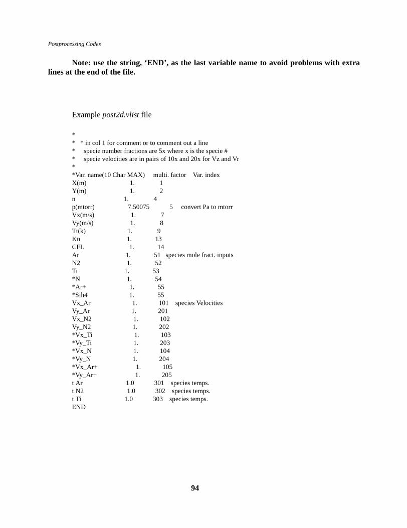
Postprocessing Codes
Note: use the string, ‘END’, as the last variable name to avoid problems with extralines at the end of the file.
Example post2d.vlist file
** * in col 1 for comment or to comment out a line* specie number fractions are 5x where x is the specie #* specie velocities are in pairs of 10x and 20x for Vz and Vr**Var. name(10 Char MAX) multi. factor Var. indexX(m) 1. 1Y(m) 1. 2 n 1. 4p(mtorr) 7.50075 5 convert Pa to mtorrVx(m/s) 1. 7Vy(m/s) 1. 8Tt(k) 1. 9Kn 1. 13CFL 1. 14Ar 1. 51 species mole fract. inputsN2 1. 52 Ti 1. 53*N 1. 54*Ar+ 1. 55*Sih4 1. 55Vx_Ar 1. 101 species VelocitiesVy_Ar 1. 201Vx_N2 1. 102Vy_N2 1. 202*Vx_Ti 1. 103*Vy_Ti 1. 203*Vx_N 1. 104*Vy_N 1. 204*Vx_Ar+ 1. 105*Vy_Ar+ 1. 205t Ar 1.0 301 species temps.t N2 1.0 302 species temps.t Ti 1.0 303 species temps.END
94

Postprocessing Codes
8.2 Surface Information (surface2d)
Goal: Converts boundary cell information to surface fluxes and reactant fluxes (etchantflux).
Usage:surface2d arg1 arg2 arg3 arg4 arg5 arg6arg1: input file (surface.xx from Icarus)arg2: output file namearg3: if ’u’ or ’U’, file in unformatted modearg4: number of regions to extract surface data forarg5: region numbersarg6: surface material number to limit data mining
example: surface2d surf.100 surf100 x 2 1 3 4( 2 regions (3 & 4), material 4)
(note: region #’s to plot and material #s from geometry.inp file)
Other Input Files:datap
Variables:1 X or Z first dimension, X or Z (m)2 Y or R second dimension, Y or R (m)3 P surface pressure (pascals)4 shear surface shear stress (N/m2)5 qwall surface heat flux (W/m2)6 avg. hitsaverage number of particle-surface collisions per time step7 tot. hitstotal number of particle-surface collision in sample
7+1 I spec1 incident flux for species 1 (#/m2-s)7+2 I spec2 incident flux for species 2 (#/m2-s)
7+i+1 R spec1surface reaction flux for species 1 (#/m^2-s)7+i+2 R spec2surface reaction flux for species 2 (#/m^2-s)
Note: spec1 and spec2 will be replaced with their respective character strings from thespec file.
95

Postprocessing Codes
8.3 Wafer Information (waferxy2d)
Goal: Convert boundary wafer cell statistics to incident angular and energy distributions.
Usage:waferxy2d wafer.* waferout
wafer.* from icarus code (i.e. wafer.1000)waferout in Tecplot format(the surface cells designated as ‘wafer’ are defined in the geometry.inp file.)
Other Input Files:
datap
Variables:1first dimension, X or Z (m)2 second dimension, Y or R (m)3 delta angle increment, dAng (deg)
4 normalized angular distribution function for species 1 (A spec1)5 normalized angular distribution function for species 2 (A spec2)..3+i normalized angular distribution function for species i (A speci)
3+i+1 delta energy increment for species 1, del1 (eV) (dE spec1)3+i+2 normalized energy distribution function for species i, eng1 (E spec1)..
note: spec1, spec2, and speci will be replaced with their respective character strings fromspec file
to plot normalized angular distributions:select variable 3 for the x plot variableselect variable 4 - 3+i for the y plot variable
to plot normalized energy distributions:
96

Postprocessing Codes
select variable 3+i+1 for the x plot variable for species 1select variable 3+i+2 for the y plot variable for species 1
Note: The reason for this data structure is that all species have the same angular incrementfor
the angular distribution function (1 degree for axisymmetric systems and 2 degrees forcartesian).
However, each species can have its own range of energy distribution function: 0 to X ev. The output data is normalized by species for both the angular and energy distributions.
97

Postprocessing Codes
8.4 Cell Convergence Statistics (stat2d)NOT CURRENTLY OPERATIONAL FOR CURRENT TECPLOT BINARY FORMAT
Usage: stat2d cell.* cell.**
cell.*: 2d tecplot binary of dsmc solution at time 1 cell.**: 2d tecplot binary of dsmc solution at time 2
the order of file1 and file2 is not important.
Other input files: post2d.vlist: for each variable in column 3 (third variable after variable name)
0- skip variable1- obtain statistics for variable note: is standard default post2d.vlist is used, no variables are marked
Output files: stat.out - A text file with following info for each region and globally. min(%) = percent change in the min value of a variable between solution planes.
max(%) = percent change in the max value of a variable between solution planes. mean(%) = mean percent change in a variable between solution planes. standard deviation = the standard deviation of the change in a variable between solu-
tion time planes.
stat.tec - A text file which can be read into tecplot. The stat.tec file allows the min(%),max(%), mean(%) and standard deviation of a variable to be plotted versusregion number.
98

9.0 Install/Compile Software
9.1 Make filesThe Icarus code and the utilities are in a directory structure under the directory, icarus.
./icarus/code- source code for Icarus (DSMC)
./icarus/code/util- source codes for utility programs: init2d, post2d,....
./icarus/samples - sample problem files (see appendix B)
./icarus/documentation - pdf file of this document
To compile the Icarus (DSMC) code: note: the Blas library is used in the Poisson solver routine. Machine compiled libraries are available for Windows using the Absoft (mkl_c.lib) or Visual Fortran Compilers (mkl_s.lib). The source for Blas is provided if case local versions of blas.lib are not available. If electro-static fields computed using a Poisson solver are not required, one can simply comment out the calls to the Blasroutines found in poisson.f
cd ./icarus/code
make help (to see the various options)$ make help
Type "make target" where target is one of: aixmp (for IBM SP with ppe/poe) ncube (for nCUBE-2 w/MPI) ncubeg (for nCUBE-2 w/MPI -g option) mos (for Intel Paragon w/ SUNMOS MPI) tflop (for Intel Tflop w/ MPI) pcmpi (for PC/NT w/MPI - Dec Fortran) pcmpig (for PC/NT w/MPI: -g -C Dec Fortran) pc (for PC/NT 1p - Absoft) pcg (for PC/NT 1p -g -C option - Absoft) pcg2 (for PC/NT 1p -g option - Absoft) pcdec (for PC/NT 1p - Dec Fortran) pcdecg (for PC/NT 1p: -g -C option Dec Fortran) sun (for Sun 1p) sung (for Sun 1p w/ -g -C option) sunmpi (for Sun w/MPI) sunmpig (for Sun w/MPI w/-g option)
99

Install/Compile Software
To install the utility codes:cd ./icarus/code/util
for UNIX systems:
make sunV (for SUN Solaris)ormake sunos (for SUN SUNOS)ormake sgi (for SGI)ormake hp (for HP ) ormake ibm (for IBM RS6000)
for PCs, for each package (init2d, decomp2d, post2d, surface2d, etc)
make -f makepc init2d --- uses the Absoft Fortran compilermake -f makepc init2dg --- uses te Absoft Fortran compiler - debug optionmake -f makepc init2ddec --- uses the Visual Fortran compilermake -f makepc init2ddecg -- uses the Visual Fortran compiler - debug optionmake -f makepc post2d --- uses the Absoft Fortran compilermake -f makepc post2ddec -- uses the Fisual Fortran compilermake -f makepc restart2d -- uses the Absoft Fortran compilermake -f makepc restart2ddec -uses the Visual Fortran compilermake -f makepc regrid -- uses the Absoft Fortran compilermake -f makepc reggriddec -- uses the Visual Fortran compilermake -f makepc surface2d -- uses the Absoft Fortran compilermake -f makepc surface2ddec -uses the Visual Fortran compilermake -f makepc waferxy2d - uses the Absoft Fortran compilermake -f makepc waferxy2ddec-uses the Visual Fortran compiler
100

Install/Compile Software
9.2 param.h and init2d.h files
Icarus does not use dynamic memory allocation for its arrays since parallel computers typ-ically have defined memory resources per processor; a single program executable can be com-piled for any number of processor configurations. The particular problem memory requirementsare implemented via two parameter statement blocks: param.h for Icarus and most of the utilityprograms and init2d.h for the init2d code.
Note: Icarus and the utility programs will check for program limits write and respond withdiagnostic messages.
param.h
example mp version of param.h
integer gmre,gcon,ggrd,gmob,gmse,gmss,gpro,gbuf integer gmnre,gmrea,gmpcm,gstat,gmwaf,gmtab integer gmrx,movie,gmcp,gmcgp,gfield,maxk
parameter (gmre=10,ggrd=1000,gmse=500) parameter (gmob=200,gcon=500) parameter (gmss=6) parameter (gpro=1024,gbuf=800000) parameter (gmrea=23,gmpcm=2,gstat=9) parameter (gmwaf=50,gmtab=5,gmrx=20) parameter (movie=2,gmcgp=6,gfield=1)
parameter (icover=0, iplasma=1, ipoisson=1)
integer lmce,lmmo,lmob
c parameter (lmce=3510,lmmo=50000,lmob=250) parameter (lmce=10000,lmmo=500000,lmob=200,lmcp=1000)
parameter (eps=1.0E-6,maxk=5)
101

Install/Compile Software
The parameters which start with ‘g’ are global and apply to all processors; those whichstart with an ‘l’ apply only to a single processor. For a single processor executable, the quantitieswith the ‘l’ are the total program limits and for a MP executable, the local cell requirements aredictated by the number of processors which are used (see the output from decomp2d). (init2d out-put contains many of these quantities parameters)
gmre -max. number of grid regionsggrd -max number of grid lines gmse -max. number of surface elementsgmob -max. number of outer boundary elementsgcon -max number of region connectionsgmss -max. number of chemical speciesgpro -max number of mp processorsgbuf -size of global buffer arraygmrea -max. number of chemical and e- impact reactionsgmpcm-max number of reactant pair channels gstat -dimension of the statistics array for determining moments (use 9 for typical calcs)gmwaf -max. number of ‘wafer’ surface elementsgmtab -max. number of surface reaction tablesgmrx -max number of surface reactions per tablemovie - 2 for non-movie simulations
3 for movie simulationsgmcgp -max number of collision groups (for DSMC binary collisions)
1- for neutral calcs w/o trace speciesadd 2 for trace species (trace-full and trace-tract collsions)add 2 for plasmas (ion-neutral and ion-ion collisions)
gfield -number of electro-static fields(2 or 4)icover - 0 - no coverage model
1 - coverage model data structuresiplasma- 0 - neutral transport only
1 - neutral & ion transportipoisson-0 - Poisson equation not performed
1 - Poisson equation data structureslmce -max. number of local (or single processor) number of cellslmmo -max. number of local (or single processor) number of particleslmob -max. number of local (or single processor) number of outer boundarieslmcp -max. number of local grid corner pointseps -value to check for round-off precison (typically 1.e-6) (meters)maxk - max. number of loops to determine particle move in a single time step (5)
102

Install/Compile Software
init2d.h
example init2d.h (parameter section)
cc include for program init2d version 6.0c parameter ( m13 = 201, m24 = 201, mnc = 500000, 1 mas = 100, mie = 5000, mntab = 4, mnrx=20, 2 mmi = 50, mnvt = 1, mdsp = 10, 3 mnre= 2, mob = 1300, 4 mpcm= 2, mrea = 23, msd = m13*2+m24*2, 5 mse = 5500, msp = 10, mtbp = 4, 6 mnr = 100, mac = 50, 7 meb = 2*(m13+m24-1)*mnr, mcpt = mnr * 4, 8 mcp = 2*mnc, msce = mse, 9 mmp = 3, mccp = 2*mnc, mnb = 5000, a mng = (m13+m24+2), eps=1.e-6 )
character*130 title
typical values which may require adjustment:
m13 -max. number of grid lines along region side 1 or side 3 (number of cells + 1)m24 -max. number of grid lines along region side 2 or side 4 (number of cells + 1)mnc -max. number of computational cellsmrea -max. number of chemical reactionsmse -max. number of surface elementsmsp -max. number of chemical speciesmnr -max. number of grid regions
103

Install/Compile Software
9.3 MPIIcarus, V10, has been written to use the MPI parallel communication protocol. MPI li-
braries can be obtained on the web for Unix based system. The commercial product, MPI-Pro,from MPI Software Technology, has been successfully used on NT and W2000 single, quad, andcluster configurations by the authors. A simple, single processor emulation set of routines isfound in ’single.f’ and is used routinely by the authors when using a symbolic debugger. Obtain-ing MPI libraries are the users’ responsibility.
104

10.0 Miscellaneous Information
10.1 Important Relationships
Conversions:1 Pascal (N/m2) = 7.50075 mtorr1 sccm = 4.48•1017 # molecules/s1 bar = 105 Pa = 0.9869 atm1 mtorr = 0.133 Pa
Sonic Orifice:
T* = (2 / (γ+1)) ToV* = (γ R T*) 1/2
where: T* = temperature at sonic planeV* = velocity at sonic planTo = stagnation temperatureγ = ratio of specific heats (1.4 for air)R = ideal gas constant
R = R/mR = 8.3144 N-m/gmole-Km = molecular wt
(note: multiply by 1000 for MKS units, kg)
105

Miscellaneous Information
10.2 Chemical Species Database.*Values from transport chemkin, origin of transport properties not clear*Values include those from Bird’s DSMC Book*effective diameter calculated at 300 K.*viscosity coefficient fit from (default @ 273-500 K). -- mu ~ T^s, where s =visc.index* file created 19 Dec. 1994 -- J. E. Johannes - SNL*******************************************************************************************Species Charge Atomic Molecular Diameter visc Rot. Rel. # Rot.Deg. Vib. Rel. Vib. Temp.* wt(Kg) wt (m) index Coll. # Freedom Coll. # (K)******************************************************************************************* AR 0.0 .6633E-25 39.95 .3555E-09 0.8100 5.0 0.0 0.0 0. AS 0.0 .1244E-24 74.92 .7777E-09 0.8968 5.0 0.0 0.0 0. AS2 0.0 .2488E-24 149.84 .9356E-09 0.8968 5.0 2.0 0.0 0. ASH 0.0 .1261E-24 75.93 .4831E-09 0.8734 5.0 0.0 0.0 0. ASH2 0.0 .1277E-24 76.94 .4945E-09 0.9107 5.0 0.0 0.0 0. ASH3 0.0 .1294E-24 77.95 .5051E-09 0.9433 5.0 0.0 0.0 0. C 0.0 .1994E-25 12.01 .3232E-09 0.6902 5.0 0.0 0.0 0. C2 0.0 .3988E-25 24.02 .3678E-09 0.7246 5.0 2.0 0.0 0. C2H 0.0 .4156E-25 25.03 .4748E-09 0.8855 5.0 0.0 0.0 0. C2H2 0.0 .4323E-25 26.04 .4748E-09 0.8856 5.0 0.0 0.0 0. C2H3 0.0 .4490E-25 27.05 .4748E-09 0.8856 5.0 0.0 0.0 0. C2H4 0.0 .4658E-25 28.05 .4934E-09 0.9631 5.0 0.0 0.0 0. C2H5 0.0 .4825E-25 29.06 .5204E-09 0.9349 5.0 0.0 0.0 0. C2H6 0.0 .4993E-25 30.07 .5204E-09 0.9349 5.0 0.0 0.0 0. C2N 0.0 .6314E-25 38.03 .4541E-09 0.9138 5.0 0.0 0.0 0. C2N2 0.0 .8639E-25 52.04 .5733E-09 1.0077 5.0 0.0 0.0 0. C2O 0.0 .6645E-25 40.02 .4541E-09 0.9137 5.0 0.0 0.0 0. C3H2 0.0 .6317E-25 38.05 .4748E-09 0.8855 5.0 0.0 0.0 0. C3H2(S) 0.0 .6317E-25 38.05 .4748E-09 0.8855 5.0 0.0 0.0 0. C3H4 0.0 .6652E-25 40.07 .5756E-09 0.9346 5.0 0.0 0.0 0. C3H4P 0.0 .6652E-25 40.07 .5756E-09 0.9346 5.0 0.0 0.0 0. C3H6 0.0 .6987E-25 42.08 .6111E-09 0.9500 5.0 0.0 0.0 0. C3H8 0.0 .7321E-25 44.10 .6108E-09 0.9469 5.0 0.0 0.0 0. C4H 0.0 .8144E-25 49.05 .6858E-09 1.0234 5.0 0.0 0.0 0. C4H2 0.0 .8312E-25 50.06 .6858E-09 1.0235 5.0 0.0 0.0 0. C4H6 0.0 .8981E-25 54.09 .6851E-09 1.0118 5.0 0.0 0.0 0. C4H8 0.0 .9316E-25 56.11 .6852E-09 1.0234 5.0 0.0 0.0 0. C5H2 0.0 .1031E-24 62.07 .6858E-09 1.0235 5.0 0.0 0.0 0. C5H5 0.0 .1081E-24 65.10 .6858E-09 1.0235 5.0 0.0 0.0 0. C6H2 0.0 .1230E-24 74.08 .6858E-09 1.0235 5.0 0.0 0.0 0. C6H5 0.0 .1280E-24 77.11 .7367E-09 1.0526 5.0 0.0 0.0 0. C6H5(L) 0.0 .1280E-24 77.11 .7367E-09 1.0526 5.0 0.0 0.0 0. C6H5O 0.0 .1546E-24 93.11 .7760E-09 1.0658 5.0 0.0 0.0 0. C6H6 0.0 .1297E-24 78.11 .7367E-09 1.0526 5.0 0.0 0.0 0. C6H7 0.0 .1314E-24 79.12 .7367E-09 1.0525 5.0 0.0 0.0 0. CH 0.0 .2162E-25 13.02 .2726E-09 0.6933 5.0 2.0 0.0 0. CH2 0.0 .2329E-25 14.03 .4087E-09 0.7845 5.0 0.0 0.0 0. CH2(S) 0.0 .2329E-25 14.03 .4087E-09 0.7845 5.0 0.0 0. 0.0 CH2CHCCH 0.0 .8646E-25 52.08 .6858E-09 1.0235 5.0 0.0 0.0 0. CH2CHCCH2 0.0 .8814E-25 53.08 .6858E-09 1.0235 5.0 0.0 0.0 0.
106

Miscellaneous Information
CH2CHCH2 0.0 .6819E-25 41.07 .5907E-09 0.9392 5.0 0.0 0.0 0. CH2CHCHCH 0.0 .8814E-25 53.08 .6858E-09 1.0235 5.0 0.0 0.0 0. CH2(CH)2CH2 0.0 .8981E-25 54.09 .6858E-09 1.0235 5.0 0.0 0.0 0. CH2CO 0.0 .6980E-25 42.04 .5553E-09 1.0614 5.0 0.0 0.0 0. CH2O 0.0 .4985E-25 30.03 .5206E-09 1.0747 5.0 0.0 0.0 0. CH2OH 0.0 .5153E-25 31.03 .5164E-09 1.0386 5.0 0.0 0.0 0. CH3 0.0 .2496E-25 15.04 .4093E-09 0.7969 5.0 0.0 0.0 0. CH3CC 0.0 .6485E-25 39.06 .5756E-09 0.9345 5.0 0.0 0.0 0. CH3CCCH2 0.0 .8814E-25 53.08 .6851E-09 1.0118 5.0 0.0 0.0 0. CH3CCCH3 0.0 .8981E-25 54.09 .6851E-09 1.0118 5.0 0.0 0.0 0. CH3CCH2 0.0 .6819E-25 41.07 .5911E-09 0.9435 5.0 0.0 0.0 0. CH3CH2CCH 0.0 .8981E-25 54.09 .6851E-09 1.0118 5.0 0.0 0.0 0. CH3CHCH 0.0 .6819E-25 41.07 .5911E-09 0.9435 5.0 0.0 0.0 0. CH3CO 0.0 .7147E-25 43.05 .5539E-09 1.0353 5.0 0.0 0.0 0. CH3O 0.0 .5153E-25 31.03 .5150E-09 1.0120 5.0 0.0 0.0 0. CH3OH 0.0 .5320E-25 32.04 .5194E-09 1.0386 5.0 0.0 0.0 0. CH4 0.0 .2664E-25 16.04 .4022E-09 0.8400 5.0 0.0 0.0 0. CL 0.0 .5886E-25 35.45 .3831E-09 0.7762 5.0 0.0 0.0 0. CL+ 1.0 .5886E-25 35.45 .3831E-09 0.7762 5.0 0.0 0.0 0. CL- -1.0 .5886E-25 35.45 .3831E-09 0.7762 5.0 0.0 0.0 0. CL2+ 1.0 .1177E-25 70.91 .5405E-09 1.0100 5.0 2.0 0.0 0. CL2 0.0 .1177E-24 70.91 .5405E-09 1.0100 5.0 2.0 0.0 0. CN 0.0 .4320E-25 26.02 .3798E-09 0.6942 5.0 2.0 0.0 0. CNN 0.0 .6645E-25 40.02 .4541E-09 0.9138 5.0 0.0 0.0 0. CO 0.0 .4651E-25 28.01 .3710E-09 0.7254 5.0 2.0 0.0 0. CO2 0.0 .7307E-25 44.01 .4516E-09 0.9264 5.0 0.0 0.0 0. e -1 .9049E-30 0.00 .6941E-07 0.9523 5.0 0.0 0.0 0. F 0.0 .3154E-25 19.00 .2728E-09 0.7005 5.0 0.0 0.0 0. F2 0.0 .6309E-25 38.00 .3477E-09 0.7680 5.0 2.0 0.0 0. GA 0.0 .1158E-24 69.72 .9372E-09 0.8264 5.0 0.0 0.0 0. GAH 0.0 .1174E-24 70.73 .5515E-09 1.0002 5.0 2.0 0.0 0. GAME 0.0 .1407E-24 84.76 .8246E-09 0.9151 5.0 0.0 0.0 0. GAME2 0.0 .1657E-24 99.79 .8123E-09 1.0043 5.0 0.0 0.0 0. GAME3 0.0 .1906E-24 114.83 .7414E-09 1.0208 5.0 0.0 0.0 0. H 0.0 .1674E-26 1.01 .2211E-09 0.7984 5.0 0.0 0.0 0. H2 0.0 .3347E-26 2.02 .2701E-09 0.6700 5.0 2.0 0.0 0. H2C4O 0.0 .1097E-24 66.06 .6851E-09 1.0118 5.0 0.0 0.0 0. H2CCC 0.0 .6317E-25 38.05 .4748E-09 0.8855 5.0 0.0 0.0 0. H2CCC(S) 0.0 .6317E-25 38.05 .4748E-09 0.8855 5.0 0.0 0.0 0. H2CCCCCH 0.0 .1047E-24 63.08 .6851E-09 1.0118 5.0 0.0 0.0 0. H2CCCCH 0.0 .8479E-25 51.07 .6851E-09 1.0118 5.0 0.0 0.0 0. H2CCCCH2 0.0 .8646E-25 52.08 .6851E-09 1.0119 5.0 0.0 0.0 0. H2CCCH 0.0 .6485E-25 39.06 .5756E-09 0.9345 5.0 0.0 0.0 0. H2CN 0.0 .4654E-25 28.03 .5424E-09 1.0303 5.0 0.0 0.0 0. H2NO 0.0 .5317E-25 32.02 .3636E-09 0.7535 5.0 0.0 0.0 0. H2O 0.0 .2991E-25 18.02 .4387E-09 1.0855 5.0 0.0 0.0 0. H2O2 0.0 .5647E-25 34.01 .3555E-09 0.7310 5.0 0.0 0.0 0. H2S 0.0 .5658E-25 34.08 .4551E-09 0.9799 5.0 0.0 0.0 0. H2SISIH2 0.0 .9996E-25 60.20 .5875E-09 0.9862 5.0 0.0 0.0 0. H3SISIH 0.0 .9996E-25 60.20 .5875E-09 0.9862 5.0 0.0 0.0 0. HCCCHCCH 0.0 .1047E-24 63.08 .6858E-09 1.0235 5.0 0.0 0.0 0.
107

Miscellaneous Information
HCCHCC 0.0 .8479E-25 51.07 .6858E-09 1.0235 5.0 0.0 0.0 0. HCCO 0.0 .6812E-25 41.03 .2707E-09 0.7924 5.0 0.0 0.0 0. HCCOH 0.0 .6980E-25 42.04 .5553E-09 1.0614 5.0 0.0 0.0 0. HCL 0.0 .6054E-25 36.46 .4396E-09 0.9953 5.0 2.0 0.0 0. HCN 0.0 .4487E-25 27.03 .5452E-09 1.0774 5.0 0.0 0.0 0. HCNO 0.0 .7143E-25 43.03 .4537E-09 0.9067 5.0 0.0 0.0 0. HCO 0.0 .4818E-25 29.02 .5206E-09 1.0747 5.0 0.0 0.0 0. HCO+ 1.0 .4818E-25 29.02 .5206E-09 1.0748 5.0 0.0 0.0 0. HE 0.0 .6646E-26 4.00 .2157E-09 0.6330 5.0 0.0 0.0 0. HF 0.0 .3322E-25 20.01 .4598E-09 1.0871 5.0 2.0 0.0 0. HNCO 0.0 .7143E-25 43.03 .4537E-09 0.9067 5.0 0.0 0.0 0. HNNO 0.0 .7475E-25 45.02 .4537E-09 0.9067 5.0 0.0 0.0 0. HNO 0.0 .5149E-25 31.01 .3632E-09 0.7437 5.0 0.0 0.0 0. HNOH 0.0 .5317E-25 32.02 .3632E-09 0.7437 5.0 0.0 0.0 0. HO2 0.0 .5480E-25 33.01 .3555E-09 0.7311 5.0 0.0 0.0 0. HOCN 0.0 .7143E-25 43.03 .4537E-09 0.9067 5.0 0.0 0.0 0. He 0.0 .3340E-26 4.02 .2333E-09 0.6600 5.0 0.0 0.0 0. I*C3H7 0.0 .7154E-25 43.09 .6111E-09 0.9500 5.0 0.0 0.0 0. K 0.0 .6492E-25 39.10 .6944E-09 0.9523 5.0 0.0 0.0 0. K+ 1.0 .6492E-25 39.10 .6944E-09 0.9523 5.0 0.0 0.0 0. KCL 0.0 .1238E-24 74.56 .7964E-09 0.8441 5.0 2.0 0.0 0. KH 0.0 .6659E-25 40.11 .3578E-09 0.7186 5.0 2.0 0.0 0. KO 0.0 .9148E-25 55.10 .5137E-09 1.0227 5.0 2.0 0.0 0. KOH 0.0 .9316E-25 56.11 .7879E-09 0.8647 5.0 2.0 0.0 0. Kr 0.0 .1391E-24 83.80 .4760E-09 0.8000 5.0 0.0 0.0 0. N 0.0 .2326E-25 14.01 .3229E-09 0.6825 5.0 0.0 0.0 0. N*C3H7 0.0 .7154E-25 43.09 .6108E-09 0.9469 5.0 0.0 0.0 0. N2 0.0 .4651E-25 28.01 .3675E-09 0.7400 5.0 2.0 0.0 0. N2H2 0.0 .4986E-25 30.03 .3718E-09 0.6825 5.0 0.0 0.0 0. N2H3 0.0 .5153E-25 31.04 .4469E-09 0.8645 5.0 0.0 0.0 0. N2H4 0.0 .5320E-25 32.05 .4872E-09 0.8711 5.0 0.0 0.0 0. N2O 0.0 .7307E-25 44.01 .4537E-09 0.9067 5.0 0.0 0.0 0. NCN 0.0 .6645E-25 40.02 .4541E-09 0.9139 5.0 0.0 0.0 0. NCO 0.0 .6976E-25 42.02 .4541E-09 0.9139 5.0 0.0 0.0 0. NH 0.0 .2493E-25 15.01 .2628E-09 0.6989 5.0 2.0 0.0 0. NH2 0.0 .2660E-25 16.02 .2628E-09 0.6988 5.0 0.0 0.0 0. NH3 0.0 .2828E-25 17.03 .4290E-09 1.1000 5.0 0.0 0.0 0. NNH 0.0 .4818E-25 29.02 .3721E-09 0.6886 5.0 0.0 0.0 0. NO 0.0 .4982E-25 30.01 .3678E-09 0.7900 5.0 2.0 0.0 0. NO2 0.0 .7638E-25 46.01 .4014E-09 0.8733 5.0 0.0 0.0 0. Ne 0.0 .3350E-25 20.80 .2770E-09 0.6600 5.0 0.0 0.0 0. O 0.0 .2656E-25 16.00 .2727E-09 0.6989 5.0 0.0 0.0 0. O2 0.0 .5313E-25 32.00 .3558E-09 0.7700 5.0 2.0 0.0 0. O3 0.0 .7969E-25 48.00 .4601E-09 0.8455 5.0 0.0 0.0 0. OH 0.0 .2824E-25 17.01 .2727E-09 0.6988 5.0 2.0 0.0 0. S 0.0 .5324E-25 32.06 .6273E-09 0.9600 5.0 0.0 0.0 0. S2 0.0 .1065E-24 64.13 .6373E-09 0.9600 5.0 2.0 0.0 0. SH 0.0 .5491E-25 33.07 .6373E-09 0.9600 5.0 2.0 0.0 0. SI 0.0 .4663E-25 28.09 .5923E-09 0.8241 5.0 2.0 0.0 0. SI2 0.0 .9326E-25 56.17 .6676E-09 0.8241 5.0 2.0 0.0 0. SI2H2 0.0 .9661E-25 58.19 .5651E-09 0.9974 5.0 0.0 0.0 0.
108

Miscellaneous Information
SI2H3 0.0 .9828E-25 59.20 .5768E-09 0.9937 5.0 0.0 0.0 0. SI2H5 0.0 .1016E-24 61.21 .5997E-09 0.9856 5.0 0.0 0.0 0. SI2H6 0.0 .1033E-24 62.22 .6109E-09 0.9814 5.0 0.0 0.0 0. SI3 0.0 .1399E-24 84.26 .7225E-09 0.8241 5.0 0.0 0.0 0. SI3H8 0.0 .1533E-24 92.32 .7210E-09 0.9975 5.0 0.0 0.0 0. SICL2 0.0 .1647E-24 98.00 .8000E-09 0.8386 5.0 2.0 0.0 0. SICL4 0.0 .2821E-24 169.90 .5428E-09 0.8363 5.0 0.0 0.0 0. SIF3 0.0 .1413E-24 85.08 .5554E-09 0.9876 5.0 0.0 0.0 0. SIF3NH2 0.0 .1679E-24 101.10 .5894E-09 0.9122 5.0 0.0 0.0 0. SIF4 0.0 .1728E-24 104.08 .5428E-09 0.8363 5.0 0.0 0.0 0. SIH 0.0 .4830E-25 29.09 .3711E-09 0.7206 5.0 0.0 0.0 0. SIH2 0.0 .4998E-25 30.10 .4041E-09 0.7776 5.0 0.0 0.0 0. SIH3 0.0 .5165E-25 31.11 .4377E-09 0.8320 5.0 0.0 0.0 0. SIH4 0.0 .5333E-25 32.12 .4722E-09 0.8826 5.0 0.0 0.0 0. SIHF3 0.0 .1429E-24 86.09 .5258E-09 0.8485 5.0 0.0 0.0 0. SO 0.0 .7980E-25 48.06 .5051E-09 0.9811 5.0 2.0 0.0 0. SO2 0.0 .1064E-24 64.06 .5188E-09 1.0500 5.0 0.0 0.0 0. SO3 0.0 .1329E-24 80.06 .5611E-09 1.0261 5.0 0.0 0.0 0. Xe 0.0 .2180E-24 131.29 .5740E-09 0.8500 5.0 0.0 0.0 0.0
109

110
11.0 References
11.1 Bird, G. A., Molecular Gas Dynamics and the Direct Simulation of Gas Flows,Clarendon Press - Oxford, 1994.
11.2 Borgnakke, C.and P. S. Larsen, Statistical collision model for Monte Carlosimulation of polyatomic gas mixtures, J. Comp. Phys., 18, 405-420 (1975).
11.3 Hermina, W. L., Monte Carlo Simulation of Transitional Flow Around SimpleShaped Bodies, Proceedings of the 15th International Symp. on Rarefied GasDynamics, Vol. I, pp. 451-460 (1986).
11.4 Kee, R., Rupley, F., Meeks, E., and Miller, J. CHEMKIN-III: A FortranChemical Kinetics Package for the Analysis of Gas Phase Chemical andPlasma Kinetics, Sandia Report SAND96-8216.
11.5 Marriott P.M. and Harvey J.K., New Approach for Modelling Energy Exchange andChemical Reactions in the Direct Simulation Monte Carlo Method, Proceedings ofthe 17th International Symposium on Rarefied Gas Dynamics, Aachen, Germany,pp. 784-788, 1990.
11.6 Gallis M.A. and Harvey J.K., Modelling of Chemical Reactions in HypersonicRarefied Flow with the Direct Simulation Monte Carlo Method, Journal of FluidMechanics, Vol: 312, pp. 149-172, 1996.
11.7 Brebbia, C. A. and J. Dominguez, Boundary Elements, An Introductory Course,2nd ed., WIT Press/Computational Mechanics Publications 1992.

111
12.0 Papers
12.1 Bartel, T.J. and Plimpton, S.J., DSMC Simulation of Rarefied Gas Dynamics on aLarge Hypercube Supercomputer, AIAA 92-2860, 1992.
12.2 Bartel, T.J. and Justiz, C.R., DSMC Simulation of Ionized Rarefied Flows, AIAA93-3095, 1993.
12.3 Bartel, T.J., Sterk, T.M., Payne, J.L., and Preppernau, B., DSMC Simulation ofNozzle Expansion Flow Fields, AIAA 94-2047, 1994.
12.4 Bartel, T.J., Low Density Gas Modelling in the Microelectronics Industry, 19thInternational Symp. on Rarefied Gas Dynamics-1994, Oxford University Press,1995.
12.5 Bartel, T.J. and Economou, D.J., Modelling of Plasma etching Discharges, invitedpresentation at 1994 AVS meeting, Denver.
12.6 Shufflebotham, P.K., Bartel, T.J, Berney, B., Experimental validation of a directsimulation by Monte Carlo molecular gas flow model, J. Vac. Sci. Technol. B13(4), Jul/Aug 1995.
12.7 Hudson, M. L., and Bartel, T. J., Direct simulation Monte Carlo computation ofreactor-feature scale flows, J. Vac. Sci. Technol. A 15(3), May/Jun 1997.
12.8 Johannes, J, Bartel, T., Hebner, G., Woodworth, J., and Economou, D., DirectSimulation Monte Carlo of Inductively Coupled Plasma and Comparison withExperiments, J. Electrochem. Soc., Vol. 144, No. 7, July 1997.
12.9 Roy, C., Bartel, T., Gallis, M., Payne, J., DSMC and Navier-Stokes Predictions forHypersnoic Laminar Interacting Flows, AIAA 2001-1030, 2001.
12.10 Gallis, M.A. and Torczynski, J.R., The Application of the BGK Model in ParticleSimulations, AIAA 2000-2360, Denver, 2000.
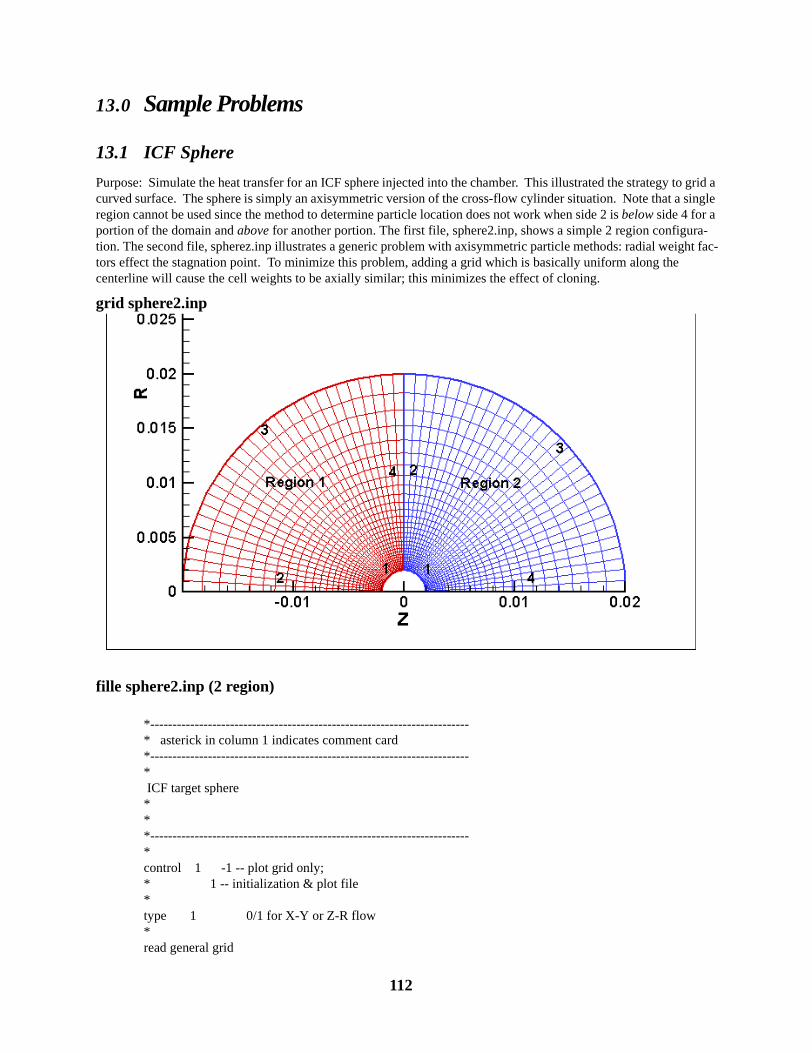
13.0 Sample Problems
13.1 ICF SpherePurpose: Simulate the heat transfer for an ICF sphere injected into the chamber. This illustrated the strategy to grid a curved surface. The sphere is simply an axisymmetric version of the cross-flow cylinder situation. Note that a single region cannot be used since the method to determine particle location does not work when side 2 is below side 4 for a portion of the domain and above for another portion. The first file, sphere2.inp, shows a simple 2 region configura-tion. The second file, spherez.inp illustrates a generic problem with axisymmetric particle methods: radial weight fac-tors effect the stagnation point. To minimize this problem, adding a grid which is basically uniform along the centerline will cause the cell weights to be axially similar; this minimizes the effect of cloning.
grid sphere2.inp
fille sphere2.inp (2 region)
*------------------------------------------------------------------------* asterick in column 1 indicates comment card*------------------------------------------------------------------------* ICF target sphere***------------------------------------------------------------------------*control 1 -1 -- plot grid only;* 1 -- initialization & plot file*type 1 0/1 for X-Y or Z-R flow*read general grid
112

Sample Problems
*----------------------------------------------------------------------* Region Definition*---------------------------------------------------------------------- 2 number of regions (must be .le. 30) 6 number of global points (must be .le.120)*--------------------------------------* Global corner pt. coordinates* Pt. z (m) r(m)*--------------------------------------1 -0.02 0.2 -0.002 0.0 3 0.002 0.04 0.02 0.05 0.0 0.0026 0.0 0.02*-----------------------------------------------------------------------* Individual Region Definitions Follow * --REGION NUMBERS MUST BE SEQUENTIAL--*-----------------------------------------------------------------------*=========================================================================region 1 <------ Inputs specific to this region follow*=========================================================================grid 2 global points 1 6 5 30 number of cells along sides 1 and 3 30 number of cells along sides 2 and 4 1 sides 1 and 3 curvature: 0/1 for line/circular arc 0 sides 1 and 3 cell spacing: 2 1.1 150. sides 2 and 4 cell spacing: 5 boundary type code for sides 1 - 4, resp. 1 3 7 3*-------------------------------------------------------------------------* Side Cell1 Cell2 elem/cell Spec. refl. Temp. K Material# Value*------------------------------------------------------------------------- 1 1 5 1 0.000 18.00 0 0. 1 6 15 3 0.000 18.00 0 0. 1 16 500 1 0.000 18.00 0 0.*-------------------------------------------------------------------------* Region interface/matching * Reg. side reg. sides Adj. side| Adj. reg.*------------------------------------------------------------------------- 1 0 2 0 3 0 4 1 2 2
113
Sample Problems
*=========================================================================*=========================================================================region 2 <------ Inputs specific to this region follow*=========================================================================grid 5 global points 6 4 3 30 number of cells along sides 1 and 3 30 number of cells along sides 2 and 4 1 sides 1 and 3 curvature: 0/1 for line/circular arc 0 sides 1 and 3 cell spacing: 2 1.1 150. sides 2 and 4 cell spacing: 5 boundary type code for sides 1 - 4, resp. 7 3 1 1*-------------------------------------------------------------------------* Side Cell1 Cell2 elem/cell Spec. refl. Temp. K Material# Value*------------------------------------------------------------------------- 1 1 500 1 0.000 18.00 0 0.*-------------------------------------------------------------------------* Region interface/matching * Reg. side reg. sides Adj. side| Adj. reg.*------------------------------------------------------------------------- 1 0 2 1 4 1 3 0 4 0 *=========================================================================*=========================================================================*-------------------------------------------------------------------------END END OF EXPERT INPUT FILE*-------------------------------------------------------------------------
file: inlet (specify freestream conditions)
** freestream inlet condition for the ICF sphere* * Xe species*1 number of tables*0 ----- flag to specify freestream conditions3.216e20 400. 0.0 1500. 1500. 1500. 1.*
114

Sample Problems
file: spec (only translational modes simulated, extra input in file)**************************************** species data file ****************************************1 number of species*3 internal structure of most complex molecule:* 3-monatomic, 4-rotation, 5-rotat. + vibrat.*0 # of chemical reactions**-------------------------------------------------------------------------------------------------------------------* ID* Mwt Mol. mass Diam. #Rot.Deg. Rot.Rel. # Vib. Deg. Vib. Rel. Vib.Temp. specie wt. charge omega tref alpha* (kg) (m) Freedom Coll. # Freedom Coll. # (K)*-------------------------------------------------------------------------------------------------------------------- Xe 131.229 2.18e-25 5.74e-10 0. 5. 0. 0. 0. 1.0 0.0 .85 300. 1.*END
O2 32.00 5.31E-26 3.96E-10 2. 5. 50. 2270. 1.0 0.0 N2 28.016 4.65E-26 4.07E-10 2. 5. 50. 3390. 1.0 0.0 O 16.00 2.65E-26 3.E-10 0. 0. 0. 0. 1.0 0.0 N 14.008 2.325E-26 3.E-10 0. 0. 0. 0. 1.0 0.0 NO 30.008 4.98E-26 4.E-10 2. 5. 50. 2740. 1.0 0.0
screen output from init2d: init2d for Icarus -- version 10.00f
opening input file sphere2.inp
opening species file spec finished with file spec
opening inlet file inlet finished reading file inlet
starting region 1 starting region 2
115

Sample Problems
total cell volume(m^3) = 3.345388E-05
values in () pertain to param.h limits
initial molecules based on 20 min per cell
34436 molecules in initial grid 2 regions (gmre) 1800 computational cells (gmce) 1 chemical species (gmss)
14 region connections (gcon) 124 grid data size (ggrd) 60 boundary elements (gmob) 80 surface elements (gmse) 1922 cell corner points (gmcp) 60 inlet table boundary cells 0 pumps or pressure points 0 # of wafer elements (gmwaf)
species definition file = spec inlet flow boundary file = inlet output grid file = grid output problem definition file = datap summary output file = init2dout
116

Sample Problems
file: spherez.inp (zoomed view)
*------------------------------------------------------------------------* asterick in column 1 indicates comment card*------------------------------------------------------------------------* 1/2 sphere***------------------------------------------------------------------------*control 1 -1 -- plot grid only;* 1 -- initialization & plot file*type 1 0/1 for X-Y or Z-R flow*read general grid*----------------------------------------------------------------------* Region Definition*---------------------------------------------------------------------- 2 number of regions (must be .le. 30) 8 number of global points (must be .le.120)*--------------------------------------
117

Sample Problems
* Global corner pt. coordinates* Pt. z (m) r(m)*--------------------------------------1 -0.02 0.2 -0.002 0.0 3 0.002 0.04 0.02 0.05 0.0 0.0026 0.0 0.027 -0.0199908 0.0002109578 -0.00198962 0.00020913*-----------------------------------------------------------------------* Individual Region Definitions Follow * --REGION NUMBERS MUST BE SEQUENTIAL--*-----------------------------------------------------------------------*=========================================================================region 1 <------ Inputs specific to this region follow*=========================================================================grid 8 global points 7 6 5 30 number of cells along sides 1 and 3 30 number of cells along sides 2 and 4 1 sides 1 and 3 curvature: 0/1 for line/circular arc 0 sides 1 and 3 cell spacing: 2 1.1 150. sides 2 and 4 cell spacing: 5 boundary type code for sides 1 - 4, resp. 7 3 3 1*-------------------------------------------------------------------------* Side Cell1 Cell2 elem/cell Spec. refl. Temp. K Material# Value*------------------------------------------------------------------------- 1 1 500 1 0.000 18.00 0 0.*-------------------------------------------------------------------------* Region interface/matching * Reg. side reg. sides Adj. side| Adj. reg.*------------------------------------------------------------------------- 1 0 2 1 4 2 3 0 4 0 *=========================================================================*=========================================================================region 2 <------ Inputs specific to this region follow*=========================================================================grid 2 global points
118
Sample Problems
1 7 8 2 number of cells along sides 1 and 3 30 number of cells along sides 2 and 4 -5 0.002 1 1 sides 1 and 3 curvature: 0/1 for line/circular arc 0 sides 1 and 3 cell spacing: 2 1.1 150. sides 2 and 4 cell spacing: 5 boundary type code for sides 1 - 4, resp. 1 3 7 1*-------------------------------------------------------------------------* Side Cell1 Cell2 elem/cell Spec. refl. Temp. K Material# Value*------------------------------------------------------------------------- 1 1 500 1 0.000 18.00 0 0.*-------------------------------------------------------------------------* Region interface/matching * Reg. side reg. sides Adj. side| Adj. reg.*------------------------------------------------------------------------- 1 0 2 0 3 0 4 1 2 1 *=========================================================================*=========================================================================*-------------------------------------------------------------------------END END OF EXPERT INPUT FILE*-------------------------------------------------------------------------
119

Sample Problems
13.2 WedgeSingle cartesian example; used for code validation experiments.
file: wedge.inp*------------------------------------------------------------------------* asterick in column 1 indicates comment card*------------------------------------------------------------------------* 10 Deg Wedge (FINE)***------------------------------------------------------------------------* options section*------------------------------------------------------------------------*control 1 -1 -- plot grid only;* 1 -- initialization & plot file*type 0 0/1 for X-Y or Z-R flow*cell weight 0*------------------------------------------------------------------------read general grid* 2 number of regions 6 number of global points *--------------------------------------* Global corner pt. coordinates
120

Sample Problems
* Pt. z (m) r(m)*--------------------------------------1 -0.001 0.2 -0.001 0.0063 0. 0.0064 0. 0.05 0.01 0.0066 0.01 0.001763269*-----------------------------------------------------------------------* Individual Region Definitions Follow * --REGION NUMBERS MUST BE SEQUENTIAL--*-----------------------------------------------------------------------*=========================================================================region 1 <------ Inputs specific to this region follow*=========================================================================grid 1 global points 2 3 4 50 number of cells along sides 1 and 3 200 number of cells along sides 2 and 4 0 sides 1 and 3 curvature: 0/1 for line/circular arc 0 sides 1 and 3 cell spacing: 0 sides 2 and 4 cell spacing: 5 boundary type code for sides 1 - 4, resp. 3 5 7 2*-------------------------------------------------------------------------* Side Cell1 Cell2 #elem/cell Spec. refl. Temp. K Material# Value*------------------------------------------------------------------------- 1 1 500 1 1.000 180.00 0 0. 3 1 500 1 1.000 180.00 0 0.*-------------------------------------------------------------------------* Region interface/matching * Reg. side reg. sides Adj. side| Adj. reg.*------------------------------------------------------------------------- 1 0 2 0 3 0 4 1 2 2 *=========================================================================*=========================================================================region 2 <------ Inputs specific to this region follow*=========================================================================grid 4 global points 3 5
121

Sample Problems
6 400 number of cells along sides 1 and 3 200 number of cells along sides 2 and 4 0 sides 1 and 3 curvature: 0/1 for line/circular arc 0 sides 1 and 3 cell spacing: 0 sides 2 and 4 cell spacing: 5 boundary type code for sides 1 - 4, resp. 7 5 3 2*-------------------------------------------------------------------------* Side Cell1 Cell2 #elem/cell Spec. refl. Temp. K Material# Value*------------------------------------------------------------------------- 1 1 500 1 1.000 180.00 0 0. 3 1 500 1 1.000 180.00 0 0.*-------------------------------------------------------------------------* Region interface/matching * Reg. side reg. sides Adj. side| Adj. reg.*------------------------------------------------------------------------- 1 0 2 1 4 1 3 0 4 0 *=========================================================================*-------------------------------------------------------------------------END END OF EXPERT INPUT FILE*-------------------------------------------------------------------------
122

Sample Problems
13.3 AIAA V&V Spherically Blunted Bi-Conic (reference 12.9)This problem illustrates the use of multiple regions to cluster cells near areas of interest. The figure shows the grid for the blunted fore-cone of the body; multiple regions are used to currectly capture the bow shock as well as the large increase in density at the surface. The input option for init2d to allow one to use a solution file (either from Icarus or a continuum code in Tecplot format) to ’test’ a candidate grid by determining the local cell Kn and time step was very useful in determining the validity of this grid. The figure shows two regions in the direction normal to the surface of the body.
------------------------------------------------------------------------* asterick in column 1 indicates comment card*------------------------------------------------------------------------* AIAA Run 31 - v3c v10 grid***------------------------------------------------------------------------*control 1 -1 -- plot grid only;* 1 -- initialization & plot file*type 1 0/1 for X-Y or Z-R flow*cell weight 3*----------------------------------------------------------------------* Region Definition*---------------------------------------------------------------------read general grid* 4 number of regions (must be .le. 30) 19 number of global points (must be .le.120)*--------------------------------------
R1
R2
R3
R4
123

Sample Problems
* Global corner pt. coordinates* Pt. z (m) r(m)*--------------------------------------1 -0.003000 0.2 0.082767 0.04295143 0.1443824 0.1309374 0.184362 0.1309375 -0.009313 0.016 0.030.0317 0.122957 0.17802 7 0.144695 0.228 0.184362 0.229 -0.014313 0.010 -0.014313 0.00811 0.000 0.012 0.003037 0.00575613 0.001318 0.01101414 0.03 0.018515 0.03 0.0310.0833216 0.099472 0.066805 0.11007 0.0814917 -0.00055 0.00000018 0.002685 0.0066719 0.030.023*-----------------------------------------------------------------------* Individual Region Definitions Follow* --REGION NUMBERS MUST BE SEQUENTIAL--*-----------------------------------------------------------------------*=========================================================================region 1 <------ Inputs specific to this region follow*=========================================================================grid 11 global points 17 18 12 2000 number of cells along sides 1 and 3 200 number of cells along sides 2 and 4 1 sides 1 and 3 curvature: 0/1 for line/circular arc 0 sides 1 and 3 cell spacing 2 1.02 100. sides 2 and 4 cell spacing 5 boundary type code for sides 1 - 4, resp. 1 7 7 1*-------------------------------------------------------------------------* Side Cell1 Cell2 #elem/cell Spec. refl. Temp. K Material# Value*------------------------------------------------------------------------- 1 1 2000 1 .000 297.22 0 0.* 3 1 500 1 1.000 180.00 0 0.*-------------------------------------------------------------------------* Region interface/matching
124

Sample Problems
* Reg. side reg. sides Adj. side| Adj. reg.*------------------------------------------------------------------------- 1 0 2 0 3 1 1 2 4 1 2 3*=========================================================================region 2 <------ Inputs specific to this region follow*=========================================================================grid 17 global points 1 13 18 1000 number of cells along sides 1 and 3 250 number of cells along sides 2 and 4 1 sides 1 and 3 curvature: 0/1 for line/circular arc 0 0 2 1.03 1000 7 boundary type code for sides 1 - 4, resp. 1 3 7 0*-------------------------------------------------------------------------* Side Cell1 Cell2 #elem/cell Spec. refl. Temp. K Material# Value*-------------------------------------------------------------------------* 1 1 1000 1 .000 297.22 0 0.* 3 1 500 1 1.000 180.00 0 0.*-------------------------------------------------------------------------* Region interface/matching* Reg. side reg. sides Adj. side| Adj. reg.*------------------------------------------------------------------------- 1 1 3 1 2 0 3 0 4 1 2 4*=========================================================================region 3 <------ Inputs specific to this region follow*=========================================================================grid 12 global points 18 19 14 2000 number of cells along sides 1 and 3 200 number of cells along sides 2 and 4 0 sides 1 and 3 curvature: 0/1 for line/circular arc 0 sides 1 and 3 cell spacing: 0 sides 2 and 4 cell spacing: 5 boundary type code for sides 1 - 4, resp.
125
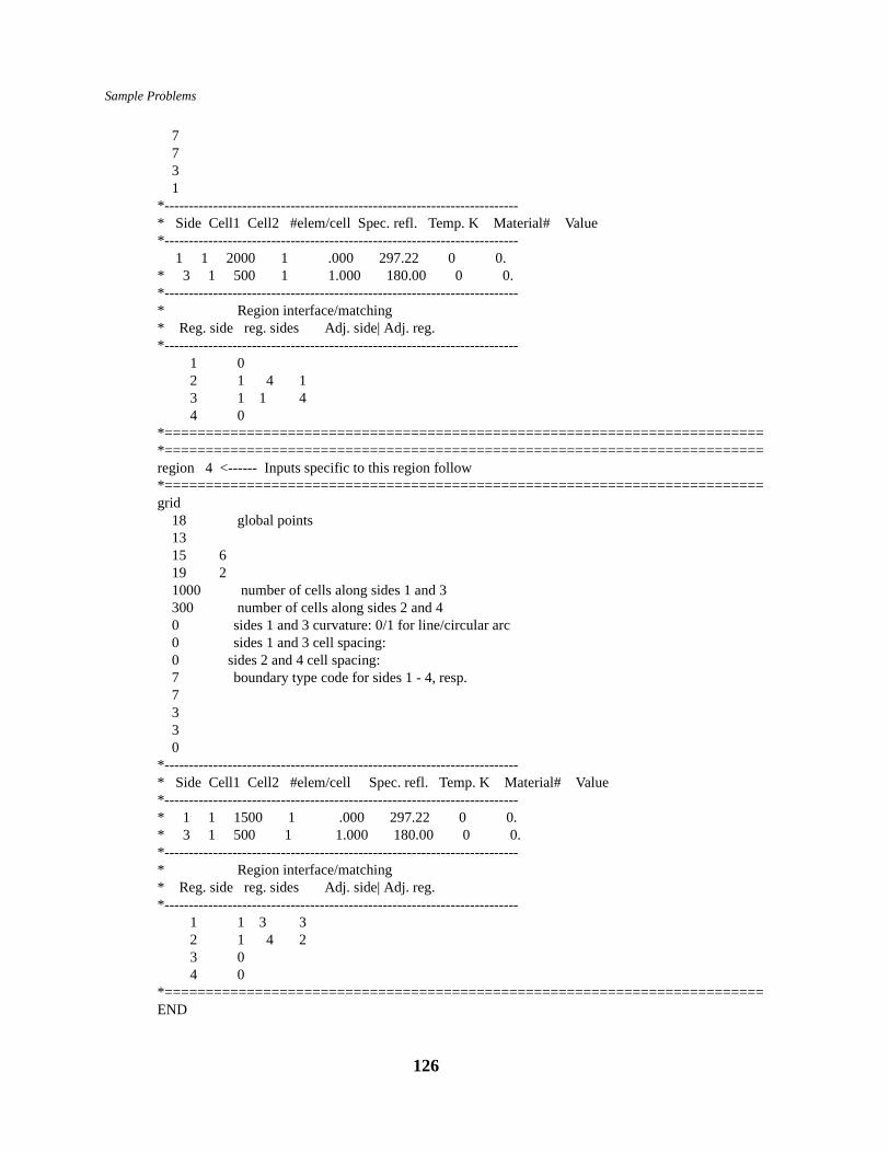
Sample Problems
7 7 3 1*-------------------------------------------------------------------------* Side Cell1 Cell2 #elem/cell Spec. refl. Temp. K Material# Value*------------------------------------------------------------------------- 1 1 2000 1 .000 297.22 0 0.* 3 1 500 1 1.000 180.00 0 0.*-------------------------------------------------------------------------* Region interface/matching* Reg. side reg. sides Adj. side| Adj. reg.*------------------------------------------------------------------------- 1 0 2 1 4 1 3 1 1 4 4 0*=========================================================================*=========================================================================region 4 <------ Inputs specific to this region follow*=========================================================================grid 18 global points 13 15 6 19 2 1000 number of cells along sides 1 and 3 300 number of cells along sides 2 and 4 0 sides 1 and 3 curvature: 0/1 for line/circular arc 0 sides 1 and 3 cell spacing: 0 sides 2 and 4 cell spacing: 7 boundary type code for sides 1 - 4, resp. 7 3 3 0*-------------------------------------------------------------------------* Side Cell1 Cell2 #elem/cell Spec. refl. Temp. K Material# Value*-------------------------------------------------------------------------* 1 1 1500 1 .000 297.22 0 0.* 3 1 500 1 1.000 180.00 0 0.*-------------------------------------------------------------------------* Region interface/matching* Reg. side reg. sides Adj. side| Adj. reg.*------------------------------------------------------------------------- 1 1 3 3 2 1 4 2 3 0 4 0*=========================================================================END
126

Sample Problems
13.4 Plasma Charge TestThis is a test problem to test the Poisson solver. The geometry is a box with the potential of the right side set to 0V and the left side set to 100kV. The top is a Neuman BC. For the axisymmetric case (chargezr.inp), the bottom is the line of symmetry and is not specifiec; for the cartesian case (chargexy.inp), the bottom BC is also Neuman. Two Icarus input run files are given: dsmc.1_laplace specifies a LaPlace solution (no volume charge density) and dsmc.1_poisson specifies a Poisson solution (constant volume charge defined in the input file.
chargezr.inp*------------------------------------------------------------------------* asterick in column 1 indicates comment card*------------------------------------------------------------------------* space charge test problem****------------------------------------------------------------------------*control 1 -1 -- plot grid only;* 1 -- initialization & plot file*
127
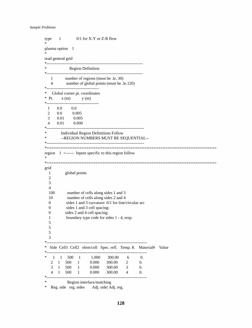
Sample Problems
type 1 0/1 for X-Y or Z-R flow*plasma option 1 *read general grid*----------------------------------------------------------------------* Region Definition*---------------------------------------------------------------------- 1 number of regions (must be .le. 30) 4 number of global points (must be .le.120)*--------------------------------------* Global corner pt. coordinates* Pt. x (m) y (m)*-------------------------------------- 1 0.0 0.0 2 0.0 0.005 3 0.01 0.005 4 0.01 0.000*-----------------------------------------------------------------------* Individual Region Definitions Follow * --REGION NUMBERS MUST BE SEQUENTIAL--*-----------------------------------------------------------------------*=========================================================================region 1 <------ Inputs specific to this region follow**=========================================================================grid 1 global points 2 3 4 100 number of cells along sides 1 and 3 10 number of cells along sides 2 and 4 0 sides 1 and 3 curvature: 0/1 for line/circular arc 0 sides 1 and 3 cell spacing: 0 sides 2 and 4 cell spacing: 1 boundary type code for sides 1 - 4, resp. 5 5 5 3*-------------------------------------------------------------------------* Side Cell1 Cell2 elem/cell Spec. refl. Temp. K Material# Value*-------------------------------------------------------------------------* 1 1 500 1 1.000 300.00 6 0. 2 1 500 1 0.000 300.00 2 0. 3 1 500 1 0.000 300.00 3 0. 4 1 500 1 0.000 300.00 4 0.*-------------------------------------------------------------------------* Region interface/matching * Reg. side reg. sides Adj. side| Adj. reg.
128
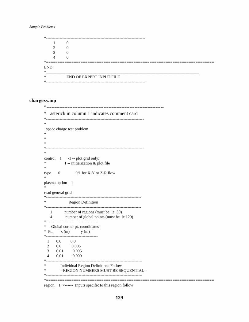
Sample Problems
*------------------------------------------------------------------------- 1 0 2 0 3 0 4 0 *========================================================================= END*___________________________________________________________________________* END OF EXPERT INPUT FILE*-------------------------------------------------------------------------
chargexy.inp*------------------------------------------------------------------------* asterick in column 1 indicates comment card*------------------------------------------------------------------------* space charge test problem****------------------------------------------------------------------------*control 1 -1 -- plot grid only;* 1 -- initialization & plot file*type 0 0/1 for X-Y or Z-R flow*plasma option 1 *read general grid*----------------------------------------------------------------------* Region Definition*---------------------------------------------------------------------- 1 number of regions (must be .le. 30) 4 number of global points (must be .le.120)*--------------------------------------* Global corner pt. coordinates* Pt. x (m) y (m)*-------------------------------------- 1 0.0 0.0 2 0.0 0.005 3 0.01 0.005 4 0.01 0.000*-----------------------------------------------------------------------* Individual Region Definitions Follow * --REGION NUMBERS MUST BE SEQUENTIAL--*-----------------------------------------------------------------------*=========================================================================region 1 <------ Inputs specific to this region follow
129

Sample Problems
**=========================================================================grid 1 global points 2 3 4 100 number of cells along sides 1 and 3 50 number of cells along sides 2 and 4 0 sides 1 and 3 curvature: 0/1 for line/circular arc 0 sides 1 and 3 cell spacing: 0 sides 2 and 4 cell spacing: 5 boundary type code for sides 1 - 4, resp. 5 5 5 4*-------------------------------------------------------------------------* Side Cell1 Cell2 elem/cell Spec. refl. Temp. K Material# Value*------------------------------------------------------------------------- 1 1 500 1 0.000 300.00 3 0. 2 1 500 1 0.000 300.00 2 0. 3 1 500 1 0.000 300.00 3 0. 4 1 500 1 0.000 300.00 4 0.*-------------------------------------------------------------------------* Region interface/matching * Reg. side reg. sides Adj. side| Adj. reg.*------------------------------------------------------------------------- 1 0 2 0 3 0 4 0 *========================================================================= END*___________________________________________________________________________* END OF EXPERT INPUT FILE*-------------------------------------------------------------------------
130

Sample Problems
dsmc.1_laplace# poisson test case log file dsmc.log output screen 1 zero flag 5
efield flag 4
######charge density 5.e17Te update 5em update 1chemistry flag 0collision flag0 read definition 0.2 datapload particles 0.0adapt flag 8000 0.25time factor 0.001thermal accom 0.5output cells 1output plasma 1run 1 0
dmsc.1_poisson# poisson test case log file dsmc.log output screen 1 zero flag 5efield flag 4charge density 5.e17Te update 5em update 1chemistry flag 0collision flag0 read definition 0.2 datapload particles 0.0
adapt flag 8000 0.25time factor 0.001thermal accom 0.5output cells 1output plasma 1run 1 0
131

Sample Problems
surfbc** this file contain surface chemistry information for the* ntube - H2 chemistry * D2 D2+ D D+ e-* 1 2 3 4 5** variable order for each reaction:* (Rx type) (Species-i) (Species-r1) (Species-r2) (create prob-1) * (create prob 2) (degree of specular reflect) (Rx prob)** For type 8: type icode voltbc eps1 eps2 0. 0. 0. *3 number of material table types** material 2 voltage=100kV2 1 1.4e16 8. 1. 100000. 0. 0.0 0. 0. 0.0** material 3, mirror bc (Enormal = 0), specular3 1 1.4e16 8. 2. 0. 0. 0.0 0. 0. 0.0** material 4 voltage=0V4 1 1.4e16 8. 1. 0. 0. 0.0 0. 0. 0.0
132

Sample Problems
13.5 Plasma Screen (Ion Accelerator)This problem illustrates some of the electro-static boundary conditions. The problem is the flow of a charge neutral plasma injected on the left of the domain with a large negative potential applied to the right of the domain. The ions will be accelerated through the screen while the electrons are repelled; a meniscus is formed around the screen. The geometry also illustrates a gridding trick which minimized the number of regions: the screen is gridded as a region with solid walls. The upstream region is connected to 3 regions when have an interface porosity of 1.0 and 2 regions which are solid walls. A similar strategy is used with the downstream connecting region. Note the use of the type 9 electro-static boundary for material type 3 (in file surf_bc). Thus the surface potential boundary conditions for the screen are set on these regions rather on a flow domain region. Since a region’s unit normals are defined as into the region, we have to flag the screen boundaries as a type 9 so that the code will reflect the normal from into the screen to into the flow domain.
file: screenz.inp*------------------------------------------------------------------------* asterick in column 1 indicates comment card*------------------------------------------------------------------------* Screen - z test**------------------------------------------------------------------------*control 1 -1 -- plot grid only;* 1 -- initialization & plot file*type 0 0/1 for X-Y or Z-R flow*******options***********
133

Sample Problems
plasma option 1 read cross_section 1chemistry file chem_d2cross_section file cross_sectionsurface file surf_bcoverwrite files 1*read general grid*----------------------------------------------------------------------*---------------------------------------------------------------------- 9 number of regions (must be .le. 30) 72 number of global points (must be .le.120)*--------------------------------------* Global corner pt. coordinates* Pt. x (m) y (m)*-------------------------------------- 1 0.00250 0.00000 2 0.00250 0.00056 3 0.00304 0.00056 4 0.00304 0.00044 5 0.00304 0.00040 6 0.00304 0.00016 7 0.00304 0.00012 8 0.00304 0.00000 9 0.00320 0.00056 10 0.00320 0.00044 11 0.00320 0.00040 12 0.00320 0.00016 13 0.00320 0.00012 14 0.00320 0.00000 15 0.00400 0.00168 16 0.00400 0.00000 17 0.00275 0.00056 18 0.00275 0.00000 19 0.00340 0.00056 20 0.00340 0.00000 21 0.00275 0.00044 22 0.00275 0.00040 23 0.00275 0.00016 24 0.00275 0.00012 25 0.00340 0.00044 26 0.00340 0.00040 27 0.00340 0.00016 28 0.00340 0.00012 29 0.00250 0.00112 30 0.00304 0.00112 31 0.00304 0.00100 32 0.00304 0.00096 33 0.00304 0.00072 34 0.00304 0.00068 35 0.00320 0.00112
134

Sample Problems
36 0.00320 0.00100 37 0.00320 0.00096 38 0.00320 0.00072 39 0.00320 0.00068 40 0.00400 0.00056 41 0.00275 0.00112 42 0.00340 0.00112 43 0.00275 0.00100 44 0.00275 0.00096 45 0.00275 0.00072 46 0.00275 0.00068 47 0.00340 0.00100 48 0.00340 0.00096 49 0.00340 0.00072 50 0.00340 0.00068 51 0.00250 0.00168 52 0.00304 0.00168 53 0.00304 0.00156 54 0.00304 0.00152 55 0.00304 0.00128 56 0.00304 0.00124 57 0.00320 0.00168 58 0.00320 0.00156 59 0.00320 0.00152 60 0.00320 0.00128 61 0.00320 0.00124 62 0.00400 0.00168 63 0.00275 0.00056 64 0.00340 0.00056 65 0.00275 0.00156 66 0.00275 0.00152 67 0.00275 0.00128 68 0.00275 0.00124 69 0.00340 0.00156 70 0.00340 0.00152 71 0.00340 0.00128 72 0.00340 0.00124 *-----------------------------------------------------------------------* Individual Region Definitions Follow *-----------------------------------------------------------------------*=========================================================================region 1 <------ Inputs specific to this region follow*=========================================================================grid 1 global points 2 63 18 2 number of cells along sides 1 and 3 2 number of cells along sides 2 and 4 0 sides 1 and 3 curvature: 0/1 for line/circular arc
135

Sample Problems
0 sides 1 and 3 cell spacing: 0 sides 2 and 4 cell spacing: 5 boundary type code for sides 1 - 4, resp. 5 5 5 4*-------------------------------------------------------------------------* Side Cell1 Cell2 elem/cell Spec. refl. Temp. K Material# Value*------------------------------------------------------------------------- 1 1 20 1 1.000 300.00 0 0. 2 1 20 1 1.000 300.00 0 0. 3 1 20 1 1.000 300.00 0 0. 4 1 20 1 1.000 300.00 0 0. *-------------------------------------------------------------------------* Region interface/matching * Reg. side reg. sides Adj. side| Adj. reg.*------------------------------------------------------------------------- 1 0 2 0 3 0 4 0 *=========================================================================region 2 <------ Inputs specific to this region follow*=========================================================================grid 1 18 global points 2 63 3 8 50 number of cells along sides 1 and 3 50 number of cells along sides 2 and 4 0 sides 1 and 3 curvature: 0/1 for line/circular arc 3 1.03 30. sides 1 and 3 cell spacing: 0 sides 2 and 4 cell spacing: 5 boundary type code for sides 1 - 4, resp. -51 5 9 4*-------------------------------------------------------------------------* Side Cell1 Cell2 elem/cell Spec. refl. Temp. K Material# Value*------------------------------------------------------------------------- 1 1 100 1 1.000 300. 1 0. 2 1 100 1 1.000 300.00 2 0. 3 1 100 1 1.000 300. 1 0. 4 1 100 1 1.000 300. 8 1. *-------------------------------------------------------------------------* Region interface/matching * Reg. side reg. sides Adj. side| Adj. reg.*-------------------------------------------------------------------------
136

Sample Problems
1 0 2 0 3 0 4 5 2 9 2 -1 2 8 2 -1 2 7*=========================================================================region 3 <------ Inputs specific to this region follow*=========================================================================grid 7 global points 6 12 13 10 number of cells along sides 1 and 3 10 number of cells along sides 2 and 4 0 sides 1 and 3 curvature: 0/1 for line/circular arc 0 sides 1 and 3 cell spacing: 0 sides 2 and 4 cell spacing: 5 boundary type code for sides 1 - 4, resp. 5 5 5 4*-------------------------------------------------------------------------* Side Cell1 Cell2 elem/cell Spec. refl. Temp. K Material# Value*------------------------------------------------------------------------- 1 1 100 10 1.000 300. 3 0.0 2 1 100 5 1.000 300. 3 0.0 3 1 100 10 1.000 300. 3 0.0 4 1 100 5 1.000 300. 3 0.0*-------------------------------------------------------------------------* Region interface/matching * Reg. side reg. sides Adj. side| Adj. reg.**------------------------------------------------------------------------- 1 0 2 0 3 0 4 0*=========================================================================region 4 <------ Inputs specific to this region follow*=========================================================================grid 5 global points 4 10 11 10 number of cells along sides 1 and 3 10 number of cells along sides 2 and 4 0 sides 1 and 3 curvature: 0/1 for line/circular arc 0 sides 1 and 3 cell spacing: 0 sides 2 and 4 cell spacing:
137

Sample Problems
5 boundary type code for sides 1 - 4, resp. 5 5 5 4*-------------------------------------------------------------------------* Side Cell1 Cell2 elem/cell Spec. refl. Temp. K Material# Value*------------------------------------------------------------------------- 1 1 100 10 1.000 300. 3 0.0 2 1 100 5 1.000 300. 3 0.0 3 1 100 10 1.000 300. 3 0.0 4 1 100 5 1.000 300. 3 0.0*-------------------------------------------------------------------------* Region interface/matching * Number adj.* Reg. side reg. sides Adj. side| Adj. reg.*------------------------------------------------------------------------- 1 0 2 0 3 0 4 0*=========================================================================region 5 <------ Inputs specific to this region follow*=========================================================================grid 14 global points 9 64 20 40 number of cells along sides 1 and 3 60 number of cells along sides 2 and 4 0 sides 1 and 3 curvature: 0/1 for line/circular arc 2 1.03 30. sides 1 and 3 cell spacing: 0 sides 2 and 4 cell spacing: 5 boundary type code for sides 1 - 4, resp. 9 5 7 3*------------------------------------------------------------------------* Side Cell1 Cell2 elem/cell Spec. refl. Temp. K Material# Value*------------------------------------------------------------------------- 1 1 100 1 1.000 300.00 1 0. 2 1 100 1 1.000 300. 8 1.0 3 1 100 1 1.000 300.00 1 0.*-------------------------------------------------------------------------* Region interface/matching * Number adj.* Reg. side reg. sides Adj. side| Adj. reg.*------------------------------------------------------------------------- 1 0
138
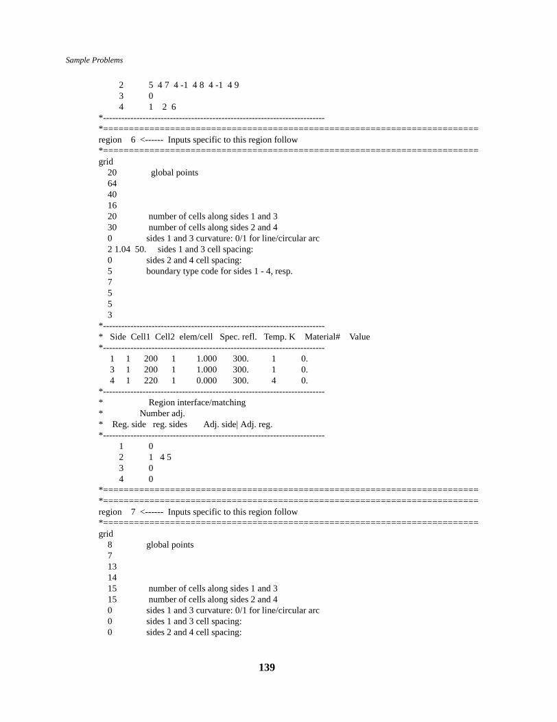
Sample Problems
2 5 4 7 4 -1 4 8 4 -1 4 9 3 0 4 1 2 6 *-------------------------------------------------------------------------*=========================================================================region 6 <------ Inputs specific to this region follow*=========================================================================grid 20 global points 64 40 16 20 number of cells along sides 1 and 3 30 number of cells along sides 2 and 4 0 sides 1 and 3 curvature: 0/1 for line/circular arc 2 1.04 50. sides 1 and 3 cell spacing: 0 sides 2 and 4 cell spacing: 5 boundary type code for sides 1 - 4, resp. 7 5 5 3*-------------------------------------------------------------------------* Side Cell1 Cell2 elem/cell Spec. refl. Temp. K Material# Value*------------------------------------------------------------------------- 1 1 200 1 1.000 300. 1 0. 3 1 200 1 1.000 300. 1 0. 4 1 220 1 0.000 300. 4 0. *-------------------------------------------------------------------------* Region interface/matching * Number adj.* Reg. side reg. sides Adj. side| Adj. reg.*------------------------------------------------------------------------- 1 0 2 1 4 5 3 0 4 0*=========================================================================*=========================================================================region 7 <------ Inputs specific to this region follow*=========================================================================grid 8 global points 7 13 14 15 number of cells along sides 1 and 3 15 number of cells along sides 2 and 4 0 sides 1 and 3 curvature: 0/1 for line/circular arc 0 sides 1 and 3 cell spacing: 0 sides 2 and 4 cell spacing:
139

Sample Problems
5 boundary type code for sides 1 - 4, resp. 7 5 7 2*-------------------------------------------------------------------------* Side Cell1 Cell2 elem/cell Spec. refl. Temp. K Material# Value*------------------------------------------------------------------------- 1 1 100 1 1.000 300. 1 0. 3 1 100 1 1.000 300. 8 0. *-------------------------------------------------------------------------* |-----> Only need if IVN > 0; then supply IVN pairs of (IVR,IVS)* Number adj.* Reg. side reg. sides Adj. side| Adj. reg.*------------------------------------------------------------------------- 1 0 2 1 4 2 3 0 4 1 2 5*=========================================================================*=========================================================================region 8 <------ Inputs specific to this region follow*=========================================================================grid 6 global points 5 11 12 25 number of cells along sides 1 and 3 25 number of cells along sides 2 and 4 0 sides 1 and 3 curvature: 0/1 for line/circular arc 0 sides 1 and 3 cell spacing: 0 sides 2 and 4 cell spacing: 5 boundary type code for sides 1 - 4, resp. 7 5 7 2*-------------------------------------------------------------------------* Side Cell1 Cell2 elem/cell Spec. refl. Temp. K Material# Value*------------------------------------------------------------------------- 1 1 100 1 1.000 300. 8 0. 3 1 100 1 1.000 300. 8 0. *-------------------------------------------------------------------------* Region interface/matching * Number adj.* Reg. side reg. sides Adj. side| Adj. reg.*------------------------------------------------------------------------- 1 0 2 1 4 2 3 0
140

Sample Problems
4 1 2 5*=========================================================================*=========================================================================region 9 <------ Inputs specific to this region follow*=========================================================================grid 4 global points 3 9 10 15 number of cells along sides 1 and 3 15 number of cells along sides 2 and 4 0 sides 1 and 3 curvature: 0/1 for line/circular arc 0 sides 1 and 3 cell spacing: 0 sides 2 and 4 cell spacing: 5 boundary type code for sides 1 - 4, resp. 7 5 7 2*-------------------------------------------------------------------------* Side Cell1 Cell2 elem/cell Spec. refl. Temp. K Material# Value*------------------------------------------------------------------------- 1 1 100 1 1.000 300. 8 0. 3 1 100 1 1.000 300. 1 0. *-------------------------------------------------------------------------* Region interface/matching * Number adj.* Reg. side reg. sides Adj. side| Adj. reg.*------------------------------------------------------------------------- 1 0 2 1 4 2 3 0 4 1 2 5*=========================================================================END************************End of Input*********************************
141
Sample Problems
file: surf_bc** this file contain surface chemistry information for the* ntube - H2 chemistry * D2 D D2+ D+ Fe- E* 1 2 3 4 5 6** variable order for each reaction:* (Rx type) (Species-i) (Species-r1) (Species-r2) (create prob-1) * (create prob 2) (degree of specular reflect) (Rx prob)** For type 8: type icode voltbc eps1 eps2 0. 0. 0. *8 number of material table types** material 1 sym. BC -- voltage=0, specular side 11 1 1.4e16 8 2. 0.0 1.0 0.0 0. 0. 0.0** material 5 sym. BC -- voltage=0, specular side 35 1 1.4e16 8 2. .0 0.0 0.0 0. 0. 0.0*****8 2. .0 3.0 0.0 0. 0. 0.0* material 2, old inlet surface file2 6 1.4e16 1. 1. 1. 0. 0.0 0. 1. 1.01. 2. 2. 0. 0.0 0. 1. 1.01. 3. 3. 0. 0.0 0. 1. 1.01. 4. 4. 0. 0.0 0. 1. 1.01. 5. 5. 0. 0.0 0. 1. 1.08. 1. 0. 0. 0.0 0. 0. 0.0** material 3, screen -- voltage bc, 3 4 1.4e16 1. 2. 2. 0. 0.0 0. 0. 1.01. 4. 2. 0. 1.0 0. 0. 1.01. 5. 5. 0. 0.0 0. 0. 1.08. 9. 0. 0. 0.0 0. 0. 0.0** material 4, ions go into target. 4 4 1.4e16 1. 2. 2. 0. 0.0 0. 0. 1.01. 4. 4. 0. 0.0 0. 0. 1.01 5. 5. 0. 0.0 0. 0. 1.0 8. 1. -10000. 0. 0.0 0. 0. 0.0* material 6, all particles stick -- inlet bc 6 3 1.4e16 1. 3. 3. 0. 0.0 0. 0. 1.01. 4. 4. 0. 0.0 0. 0. 1.01 5. 5. 0. 0.0 0. 0. 1.0 * material 7 sym. BC -- voltage=0, specular sSide 1
142

Sample Problems
7 1 1.4e16 8 1. 0.0 1.0 0.0 0. 0. 0.0*** material 8, screen -- with NO voltage bc, 8 3 1.4e16 1. 2. 2. 0. 0.0 0. 0. 1.01. 4. 2. 0. 1.0 0. 0. 1.01. 5. 5. 0. 0.0 0. 0. 1.0
143

Sample Problems
13.6 Micro-GyroscopeThis problem illustrates the use of a ’test point’ to monitor the pressure/density at a given location in the flowfield andalso the rotating boundary condition. Although this simulations is axisymmetric, one surface is rotating at a givenrotational speed, w. Thus, when a molecule hits this surface, an ’out-of-plane’ or V-theta velocity is rw, r is the localradial distance. The domain consists of 2 regions along the R axis: the first region is bounded by the centerline, afixed wall, and the rotating wall. The second region is bounded by 2 fixed walls and a line of symmetry. This systemis closed.
file: gyro.inp*------------------------------------------------------------------------* asterick in column 1 indicates comment card*------------------------------------------------------------------------* micro-gyro --- base case***------------------------------------------------------------------------* options section*------------------------------------------------------------------------*control 1 -1 -- plot grid only;* 1 -- initialization & plot file*type 1 0/1 for X-Y or Z-R flow*cell weight 4*------------------------------------------------------------------------read general grid* 2 number of regions 7 number of global points *--------------------------------------* Global corner pt. coordinates* Pt. z (m) r(m)*-------------------------------------- 1 0.0 0.0 2 0.000 500.e-6 3 0.000 750.e-6 4 1.e-6 0.00 5 1.e-6 500e-6 6 1.e-6 750.e-6 7 0.5e-6 500.e-6*read test points -1 1 7*
144

Sample Problems
*=========================================================================region 1 <------ Inputs specific to this region follow*=========================================================================grid 1 global points 2 5 4 10 number of cells along sides 1 and 3 225 number of cells along sides 2 and 4 0 sides 1 and 3 curvature: 0/1 for line/circular arc 0 sides 1 and 3 cell spacing: 0 sides 2 and 4 cell spacing: 1 boundary type code for sides 1 - 4, resp. 5 7 5 2 *-------------------------------------------------------------------------* Side Cell1 Cell2 #elem/cell Spec. refl. Temp. K Material# Value*------------------------------------------------------------------------- 2 1 300 1 0.000 300. 0 0. 4 1 700 1 0.000 300. 1 0.0*-------------------------------------------------------------------------* Region interface/matching * Reg. side reg. sides Adj. side| Adj. reg.*------------------------------------------------------------------------- 1 0 2 0 3 1 1 2 4 0*=========================================================================region 2 <------ Inputs specific to this region follow*=========================================================================grid 2 global points 3 6 5 10 number of cells along sides 1 and 3 100 number of cells along sides 2 and 4 0 sides 1 and 3 curvature: 0/1 for line/circular arc 0 sides 1 and 3 cell spacing: 0 sides 2 and 4 cell spacing: 7 boundary type code for sides 1 - 4, resp. 5 5 5 3 *-------------------------------------------------------------------------* Side Cell1 Cell2 #elem/cell Spec. refl. Temp. K Material# Value
145

Sample Problems
*------------------------------------------------------------------------- 2 1 300 1 0.000 300. 0 0. 3 1 300 1 0.000 300. 0 0. 4 1 300 1 1.000 300. 0 0.0*-------------------------------------------------------------------------* Region interface/matching * Number adj.* Reg. side reg. sides Adj. side| Adj. reg.*------------------------------------------------------------------------- 1 1 3 1 2 0 3 0 4 0*-------------------------------------------------------------------------END END OF EXPERT INPUT FILE*-------------------------------------------------------------------------
file: inlet** initial conditions for the micro-gyro* * N2 species*1 number of tables*0 ----- flag to specify initial conditions0.1212e+25 0.0 0.0 300. 300. 300. 1.*
file: surfbc** N2* 1 2 3** variable order for each reaction:* *1 number of material table types*1 1 1.0-7. 00. 0.0 16666.7 0.0 0.0 0.0 0.0
146

Sample Problems
13.7 Collisional Test in a Closed Box
Isothermal flow of nitrogen in a closed box
Purpose. While this test case does not exercise any of the sophisticated options of Icarus it is particularly useful forvalidation/verification purposes. The flowfield is a two-dimensional box with two specular and two diffuse walls,divided into 1000 cells (100 across x and 10 across y). For a pressure of 100mTorr the number density is such that themean free path is a third of the cell size. For a timestep of 10-7 all the DSMC requirements for an accurate calculationare satisfied. The test case can be ran either collisionless (by inhibiting collisions) or with collisions. In the first casethe heat and number flux to the diffuse walls can be calculated (surface files) and compared with the predictions ofcollisionless gas theory (see Bird 1994 chapter 7). In the latter case the ability of the code to achieve equilibrationbetween the internal and translational modes, and the correct heat and mass fluxes to the walls can be verified. Thecollision frequency as predicted by the code can be also calculated under conditions of perfect equilibrium. All theseproperties can also be calculated analytically (see Bird, ref. 11.1, Chapter 4) and compared with the predictions ofIcarus. Comparisons made by the authors indicate agreement better than 1%.
Z
R
0 0.0025 0.005 0.0075 0.010
0.001
0.002
0.003
0.004
0.005
0.006
0.007
0.008
0.009
Specular walls
Diffuse walls at 273K
147

Sample Problems
Input File*------------------------------------------------------------------------* asterick in column 1 indicates comment card*------------------------------------------------------------------------*100mTorr/N2***------------------------------------------------------------------------* options section*------------------------------------------------------------------------*control 1 -1 -- plot grid only;* 1 -- initialization & plot file*type 0 0/1 for X-Y or Z-R flow*cell weight 0*------------------------------------------------------------------------read general grid* 1 number of regions 4 number of global points *--------------------------------------* Global corner pt. coordinates* Pt. z (m) r(m)*--------------------------------------1 .0 .02 .0 .0013 .01 .0014 .01 .0*-----------------------------------------------------------------------* Individual Region Definitions Follow * --REGION NUMBERS MUST BE SEQUENTIAL--*-----------------------------------------------------------------------*=========================================================================region 1 <------ Inputs specific to this region follow*=========================================================================grid 1 global points 2 3 4 100 number of cells along sides 1 and 3 10 number of cells along sides 2 and 4 0 sides 1 and 3 curvature: 0/1 for line/circular arc 0 sides 1 and 3 cell spacing: 0 sides 2 and 4 cell spacing: 5 boundary type code for sides 1 - 4, resp. 5 5
148

Sample Problems
5 4*-------------------------------------------------------------------------* Side Cell1 Cell2 #elem/cell Spec. refl. Temp. K Material# Value*------------------------------------------------------------------------- 1 1 100 1 1.000 273.00 0 0. 2 1 100 1 .000 273.00 0 0. 3 1 100 1 1.000 273.00 0 0. 4 1 100 1 .000 273.00 0 0.*-------------------------------------------------------------------------* Region interface/matching * Reg. side reg. sides Adj. side| Adj. reg.*------------------------------------------------------------------------- 1 0 2 0 3 0 4 0 *=========================================================================*-------------------------------------------------------------------------END END OF EXPERT INPUT FILE*-------------------------------------------------------------------------
Inlet File*_* freestream inlet condition for the N2 box relaxation* * N2 species*1 number of tables*0 ----- flag to specify freestream conditions3.537156e21 0. 0.0 273. 273. 273. 1.*
Species File
***************************************_* new species data file *****************************************1 number of species*3 internal structure of most complex molecule:* 3-monatomic, 4-rotation, 5-rotat. + vibrat.*0 # of chem. rx. (from file chem)** *---------------------------------------------------------------------------------------------------------------* ID
149

Sample Problems
* Mwt Mol. mass Diam. #Rot.Deg. Rot.Rel. #Vit. Deg. Vib. Rel. Vib.Temp. specie wt. charge ome-ga tref alpha
* (kg) (m) Freedom Coll. # Freedom Coll. # (K)*---------------------------------------------------------------------------------------------------------------- N2 28.0 4.65E-26 4.11E-10 2. 5. 50. 5. 3371. 1.0 0.0 0.74 273. 1.0*END MUST have this line as last input line.....
150

Sample Problems
151
13.8 MBF Expansion Chamber (reference paper 12.3)The problem illustrates the use of the input from a Navier-Stokes code to provide the boundary plane at the nozzle throat. Also, the collision limiter logic, used to limit the number of test particle collisions was developed for this problem.
- Input Gases: He & C3H6O
- Chemical Species:Mwt Mass VHS diameter
He 4.004 gm/gmole 6.648 x 10⁻²⁷ kg 2.19 x 10⁻¹⁰ mC3H6O 70.91 gm/gmole 9.64 x 10⁻²⁶ kg 6.67 x 10⁻¹⁰ m
use a mixture viscosity coeficient of 0.658531 @ 273 K
- Boundary conditions:inlet: sonic choked boundary
Mole fractions: He= 1.0C3H6O= 0.0outlet: nonreentrant boundary (perfect vacuum pump)
- Surface Boundary Conditions:- 100% thermal accommodation- 100% diffuse surface reaction- Temperature of all surfaces = 232.31 K
- Surface Chemistry:no reactions
- Output:- pressure, velocity, temperature and species distribution- transient flowfield results
- Reference:
T. J. Bartel et. al., "DSMC Simulation of Nozzle Expansion Flow Fields," AIAA 94-2047, 6th AIAA/ASME Joint Thermophysics & Heat Transfer Conference, Colorado Springs, CO, 1994.
0.00 0.05 0.10 0.150.00
0.02
0.04
0.06
0.08
z (m)
zoomed area 5
3
4

Sample Problems
input file:
*------------------------------------------------------------------------* asterick in column 1 indicates comment card*------------------------------------------------------------------------* MBF - He-Acetone transient simulation***------------------------------------------------------------------------*control 1 -1 -- plot grid only;* 1 -- initialization & plot file*type 1 0/1 for X-Y or Z-R flow*cell weight -4expansion radius wt 5.08e-4**read general grid*----------------------------------------------------------------------* Region Definition*---------------------------------------------------------------------- 6 number of regions (must be .le. 30) 30 number of global points (must be .le.120)
0.000 0.002 0.004 0.006 0.008
0.0000
0.0010
0.0020
0.0030
0.0040
0.0050
0.0060
1
26
152

Sample Problems
*--------------------------------------* Global corner pt. coordinates* Pt. z (m) r(m)*-------------------------------------- 1 0.000 0.0 2 1.5875e-2 0.0 3 3.2258e-2 0.0 4 1.905e-1 0.0 5 0.0 5.08e-4 6 1.65215e-2 1.63833e-2 7 0.00 1.1811e-3 8 1.5875e-2 1.7056e-2 9 1.5875e-2 7.62e-2 10 1.905e-1 7.62e-2 11 0.01 0.01 12 0.01 0.0005 13 0.005 0.0005 14 -0.00049 0.0 15 -0.00049 0.0005 16 0.002 0.00 17 0.00 0.002 18 0.015 0.03 19 0.03 0.02 20 0.1 0.0 21 0.001 0.0 22 0.001 1.46892e-3 23 0.01 0.00* 24 0.01 1.01207e-2 24 0.01 1.0508e-2 25 0.01 1.1181e-2 26 1.5875e-2 0.0 27 -2.54e-4 0.0 28 -2.54e-4 2.54e-4 29 0.012 0.0 30 0.012 1.31811e-2*--------------------------------------*=========================================================================region 1 <------ Inputs specific to this region follow*=========================================================================grid 5 global points 7 8 6 200 number of cells along sides 1 and 3 20 number of cells along sides 2 and 4 0 sides 1 and 3 curvature:: 0/1 for line/circular arc 2 1.03 40 sides 1 and 3 cell spacing: 0 sides 2 and 4 cell spacing: 7 boundary type code for sides 1 - 4, resp. 5 5
153

Sample Problems
7 2 number of BC entries*-------------------------------------------------------------------------* Side Cell1 Cell2 elem/cell Spec. refl. Temp. K Material# Value*------------------------------------------------------------------------- 2 1 100 1 0.000 300.00 0 0. 3 1 200 1 0.000 300.00 0 0.*-------------------------------------------------------------------------**-------------------------------------------------------------------------*-------------------------------------------------------------------------* Region interface/matching * Reg. side reg. sides Adj. side Adj. reg.*-------------------------------------------------------------------------*------------------------------------------------------------------------- 1 2 3 5 3 2 2 0 3 0 4 1 1 3*=========================================================================region 2 <------ Inputs specific to this region follow*=========================================================================grid 1 global points 5 22 21 60 number of cells along sides 1 and 3 50 number of cells along sides 2 and 4 0 sides 1 and 3 curvature: 0/1 for line/circular arc 2 1.04 50 sides 1 and 3 cell spacing: 0 sides 2 and 4 cell spacing: 1 boundary type code for sides 1 - 4, resp. 7 7 7 0 number of BC entries*-------------------------------------------------------------------------* Side Cell1 Cell2 elem/cell Spec. refl. Temp. K Material# Value*-------------------------------------------------------------------------**-------------------------------------------------------------------------*-------------------------------------------------------------------------* Region interface/matching * Reg. side reg. sides Adj. side Adj. reg.*-------------------------------------------------------------------------*------------------------------------------------------------------------- 1 0 2 1 4 6 3 1 1 1 4 1 2 5
154

Sample Problems
*=========================================================================region 3 <------ Inputs specific to this region follow*=========================================================================grid 8 global points 9 20 3 80 number of cells along sides 1 and 3 60 number of cells along sides 2 and 4 0 sides 1 and 3 curvature: 0/1 for line/circular arc 0 sides 1 and 3 cell spacing: 2 1.04 50 sides 2 and 4 cell spacing: 7 boundary type code for sides 1 - 4, resp. 5 7 1 1 number of BC entries*-------------------------------------------------------------------------* Side Cell1 Cell2 elem/cell Spec. refl. Temp. K Material# Value*------------------------------------------------------------------------- 2 1 100 1 0.0 300. 0 0. *-------------------------------------------------------------------------**-------------------------------------------------------------------------*-------------------------------------------------------------------------* Region interface/matching * Reg. side reg. sides Adj. side Adj. reg.*-------------------------------------------------------------------------*------------------------------------------------------------------------- 1 2 4 5 4 1 2 0 3 1 2 4 4 0*=========================================================================region 4 <------ Inputs specific to this region follow*=========================================================================grid 20 global points coinciding w/ region corner points 1 - 4, resp. 9 10 4 80 number of cells along sides 1 and 3 50 number of cells along sides 2 and 4 0 sides 1 and 3 curvature: 0/1 for line/circular arc 0 sides 1 and 3 cell spacing: 0 sides 2 and 4 cell spacing: 1 boundary type code for sides 1 - 4, resp. 7 5 11 1 number of BC entries*-------------------------------------------------------------------------
155

Sample Problems
* Side Cell1 Cell2 elem/cell Spec. refl. Temp. K Material# Value*------------------------------------------------------------------------- 3 1 100 1 0.000 300.00 0 0.*-------------------------------------------------------------------------**-------------------------------------------------------------------------*-------------------------------------------------------------------------* Region interface/matching * Reg. side reg. sides Adj. side Adj. reg.*-------------------------------------------------------------------------*------------------------------------------------------------------------- 1 0 2 1 3 3 3 0 4 0*=========================================================================region 5 <------ Inputs specific to this region follow*=========================================================================grid 21 global points 22 6 3 200 number of cells along sides 1 and 3 100 number of cells along sides 2 and 4 0 sides 1 and 3 curvature: 0/1 for line/circular arc 0 sides 1 and 3 cell spacing: 0 sides 2 and 4 cell spacing: 1 boundary type code for sides 1 - 4, resp. 7 7 7 0 number of surface bc*-------------------------------------------------------------------------* Side Cell1 Cell2 elem/cell Spec. refl. Temp. K Material# Value*-------------------------------------------------------------------------**-------------------------------------------------------------------------*-------------------------------------------------------------------------* Region interface/matching * Reg. side reg. sides Adj. side Adj. reg.*-------------------------------------------------------------------------*------------------------------------------------------------------------- 1 0 2 1 4 2 3 1 1 1 4 1 1 3*=========================================================================region 6 <------ Inputs specific to this region follow*=========================================================================grid 27 global points
156

Sample Problems
28 5 1 60 number of cells along sides 1 and 3 50 number of cells along sides 2 and 4 0 sides 1 and 3 curvature: 0/1 for line/circular arc 0 sides 1 and 3 cell spacing: 0 sides 2 and 4 cell spacing: 1 boundary type code for sides 1 - 4, resp. -31 5 7 1 number of BC entries*-------------------------------------------------------------------------* Side Cell1 Cell2 elem/cell Spec. refl. Temp. K Material# Value*------------------------------------------------------------------------- 3 1 250 1 0.000 300.00 0 0.*-------------------------------------------------------------------------**-------------------------------------------------------------------------*-------------------------------------------------------------------------* Region interface/matching * Reg. side reg. sides Adj. side Adj. reg.*-------------------------------------------------------------------------*------------------------------------------------------------------------- 1 0 2 0 3 0 4 1 2 2*-------------------------------------------------------------------------END END OF EXPERT INPUT FILE*-------------------------------------------------------------------------
inlet file:
*1 table for the MBF nozzle(INCA-M=1.05:plane at 2.53429e-4m)-file:inlet.bc1 1 69 3 table #, # of table entries, BC type** r number density Vz Vr Tt Tr Tv fraction species 1 2* units are MKS 0.000000E+00 0.610425E+26 941.7240 0.0000 0.2323E+03 0.2323E+03 0.2323E+03 0.999 .001 0.146677E-04 0.610425E+26 941.7240 0.0000 0.2323E+03 0.2323E+03 0.2323E+03 0.999 .001 0.284893E-04 0.610423E+26 941.7250 0.0002 0.2323E+03 0.2323E+03 0.2323E+03 0.999 .001 0.415138E-04 0.610423E+26 941.7260 0.0004 0.2323E+03 0.2323E+03 0.2323E+03 0.999 .001 0.537871E-04 0.610422E+26 941.7270 0.0006 0.2323E+03 0.2323E+03 0.2323E+03 0.999 .001 0.653527E-04 0.610420E+26 941.7290 0.0008 0.2323E+03 0.2323E+03 0.2323E+03 0.999 .001 0.762515E-04 0.610420E+26 941.7290 0.0009 0.2323E+03 0.2323E+03 0.2323E+03 0.999 .001 0.865219E-04 0.610420E+26 941.7280 0.0008 0.2323E+03 0.2323E+03 0.2323E+03 0.999 .001 0.962003E-04 0.610423E+26 941.7250 0.0003 0.2323E+03 0.2323E+03 0.2323E+03 0.999 .001 0.105321E-03 0.610426E+26 941.7190 -0.0008 0.2323E+03 0.2323E+03 0.2323E+03 0.999 .001 0.113916E-03 0.610434E+26 941.7100 -0.0029 0.2323E+03 0.2323E+03 0.2323E+03 0.999 .001
157

Sample Problems
0.122016E-03 0.610443E+26 941.6970 -0.0060 0.2323E+03 0.2323E+03 0.2323E+03 0.999 .001 0.129649E-03 0.610453E+26 941.6800 -0.0103 0.2323E+03 0.2323E+03 0.2323E+03 0.999 .001 0.136843E-03 0.610467E+26 941.6630 -0.0153 0.2323E+03 0.2323E+03 0.2323E+03 0.999 .001 0.143622E-03 0.610479E+26 941.6470 -0.0207 0.2323E+03 0.2323E+03 0.2323E+03 0.999 .001 0.150012E-03 0.610486E+26 941.6370 -0.0253 0.2323E+03 0.2323E+03 0.2323E+03 0.999 .001 0.156033E-03 0.610486E+26 941.6390 -0.0278 0.2323E+03 0.2323E+03 0.2323E+03 0.999 .001 0.161709E-03 0.610474E+26 941.6600 -0.0262 0.2323E+03 0.2323E+03 0.2323E+03 0.999 .001 0.167058E-03 0.610443E+26 941.7070 -0.0182 0.2323E+03 0.2323E+03 0.2323E+03 0.999 .001 0.172100E-03 0.610387E+26 941.7910 -0.0011 0.2323E+03 0.2323E+03 0.2323E+03 0.999 .001 0.176852E-03 0.610298E+26 941.9230 0.0285 0.2323E+03 0.2323E+03 0.2323E+03 0.999 .001 0.181332E-03 0.610167E+26 942.1120 0.0741 0.2322E+03 0.2322E+03 0.2322E+03 0.999 .001 0.185555E-03 0.609987E+26 942.3720 0.1400 0.2322E+03 0.2322E+03 0.2322E+03 0.999 .001 0.189536E-03 0.609747E+26 942.7140 0.2307 0.2321E+03 0.2321E+03 0.2321E+03 0.999 .001 0.193289E-03 0.609437E+26 943.1540 0.3517 0.2320E+03 0.2320E+03 0.2320E+03 0.999 .001 0.196827E-03 0.609050E+26 943.7030 0.5090 0.2319E+03 0.2319E+03 0.2319E+03 0.999 .001 0.203309E-03 0.607992E+26 945.1890 0.9614 0.2317E+03 0.2317E+03 0.2317E+03 0.999 .001 0.206276E-03 0.607298E+26 946.1510 1.2733 0.2315E+03 0.2315E+03 0.2315E+03 0.999 .001 0.209074E-03 0.606479E+26 947.2800 1.6554 0.2313E+03 0.2313E+03 0.2313E+03 0.999 .001 0.211713E-03 0.605524E+26 948.5890 2.1188 0.2311E+03 0.2311E+03 0.2311E+03 0.999 .001 0.214203E-03 0.604427E+26 950.0980 2.6759 0.2308E+03 0.2308E+03 0.2308E+03 0.999 .001 0.216552E-03 0.603180E+26 951.8240 3.3405 0.2305E+03 0.2305E+03 0.2305E+03 0.999 .001 0.218769E-03 0.601783E+26 953.7870 4.1280 0.2301E+03 0.2301E+03 0.2301E+03 0.999 .001 0.220861E-03 0.600232E+26 956.0070 5.0556 0.2297E+03 0.2297E+03 0.2297E+03 0.999 .001 0.222836E-03 0.598528E+26 958.4950 6.1421 0.2292E+03 0.2292E+03 0.2292E+03 0.999 .001 0.224701E-03 0.596664E+26 961.2550 7.4077 0.2287E+03 0.2287E+03 0.2287E+03 0.999 .001 0.226462E-03 0.594633E+26 964.2800 8.8731 0.2281E+03 0.2281E+03 0.2281E+03 0.999 .001 0.228126E-03 0.592422E+26 967.5460 10.5587 0.2275E+03 0.2275E+03 0.2275E+03 0.999 .001 0.229699E-03 0.590004E+26 971.0140 12.4847 0.2268E+03 0.2268E+03 0.2268E+03 0.999 .001 0.231185E-03 0.587356E+26 974.6250 14.6690 0.2260E+03 0.2260E+03 0.2260E+03 0.999 .001 0.232591E-03 0.584444E+26 978.3060 17.1268 0.2253E+03 0.2253E+03 0.2253E+03 0.999 .001 0.233921E-03 0.581242E+26 981.9660 19.8690 0.2245E+03 0.2245E+03 0.2245E+03 0.999 .001 0.235181E-03 0.577728E+26 985.5060 22.8939 0.2237E+03 0.2237E+03 0.2237E+03 0.999 .001 0.236373E-03 0.573890E+26 988.8250 26.1895 0.2230E+03 0.2230E+03 0.2230E+03 0.999 .001 0.237504E-03 0.569716E+26 991.8270 29.7463 0.2224E+03 0.2224E+03 0.2224E+03 0.999 .001 0.238576E-03 0.565195E+26 994.4260 33.5554 0.2218E+03 0.2218E+03 0.2218E+03 0.999 .001 0.239593E-03 0.560317E+26 996.5400 37.6030 0.2213E+03 0.2213E+03 0.2213E+03 0.999 .001 0.240560E-03 0.555077E+26 998.0970 41.8680 0.2210E+03 0.2210E+03 0.2210E+03 0.999 .001 0.241479E-03 0.549471E+26 999.0400 46.3152 0.2207E+03 0.2207E+03 0.2207E+03 0.999 .001 0.242354E-03 0.543508E+26 999.3340 50.8990 0.2206E+03 0.2206E+03 0.2206E+03 0.999 .001 0.243188E-03 0.537218E+26 998.9510 55.5788 0.2206E+03 0.2206E+03 0.2206E+03 0.999 .001 0.243983E-03 0.530613E+26 997.8610 60.3215 0.2208E+03 0.2208E+03 0.2208E+03 0.999 .001 0.244743E-03 0.523698E+26 996.0320 65.0949 0.2210E+03 0.2210E+03 0.2210E+03 0.999 .001 0.245471E-03 0.516481E+26 993.4200 69.8661 0.2215E+03 0.2215E+03 0.2215E+03 0.999 .001 0.246168E-03 0.508962E+26 989.9740 74.6020 0.2221E+03 0.2221E+03 0.2221E+03 0.999 .001 0.246838E-03 0.501135E+26 985.6220 79.2665 0.2229E+03 0.2229E+03 0.2229E+03 0.999 .001 0.247482E-03 0.492995E+26 980.2630 83.8187 0.2238E+03 0.2238E+03 0.2238E+03 0.999 .001 0.248103E-03 0.484526E+26 973.7540 88.2192 0.2250E+03 0.2250E+03 0.2250E+03 0.999 .001 0.248703E-03 0.475739E+26 965.8640 92.4555 0.2264E+03 0.2264E+03 0.2264E+03 0.999 .001 0.249285E-03 0.466683E+26 956.2080 96.5942 0.2281E+03 0.2281E+03 0.2281E+03 0.999 .001 0.249850E-03 0.457380E+26 944.3170 100.7240 0.2302E+03 0.2302E+03 0.2302E+03 0.999 .001 0.250400E-03 0.447682E+26 929.7660 104.6890 0.2327E+03 0.2327E+03 0.2327E+03 0.999 .001
158

Sample Problems
0.250938E-03 0.437375E+26 911.8630 107.9540 0.2358E+03 0.2358E+03 0.2358E+03 0.999 .001 0.251465E-03 0.426346E+26 889.0870 109.7260 0.2395E+03 0.2395E+03 0.2395E+03 0.999 .001 0.251982E-03 0.414573E+26 858.6020 108.9840 0.2439E+03 0.2439E+03 0.2439E+03 0.999 .001 0.252493E-03 0.402026E+26 815.4470 103.9530 0.2494E+03 0.2494E+03 0.2494E+03 0.999 .001 0.252998E-03 0.388550E+26 750.9500 90.3279 0.2560E+03 0.2560E+03 0.2560E+03 0.999 .001 0.253500E-03 0.374430E+26 649.8740 57.8191 0.2628E+03 0.2628E+03 0.2628E+03 0.999 .001 0.254000E-03 0.311123E+26 0.0000 0.0000 0.3000E+03 0.3000E+03 0.3000E+03 0.999 .001
Icarus input file:
# MBF - He-Acetone (0.001) t1
log file dsmc.log
output screen100
zero flag20
read def 1.0 datap
adapt flag 200 0.25time factor 0.001
output cell 1000output surf 5000
run 20000 0
159

Sample Problems
13.9 NO Nozzle Expansion and Data Comparison (reference paper 12.2)This problem illustrates how the choice of grid regions and cell clustering can be chosen to improve the accurary of the simulation.
- Input Gases: NO
- Boundary conditions:inlet: 25 torr pulsed valve (radial inlet)outlet: vacuum
- Surface Boundary Conditions:- 100% thermal accommodation- 100% diffuse surface reaction- Temperature of all surfaces = 373 K
- Output:- rotational temperature, density and pressure
- Reference:
Bartel, T. J. & Justiz, C. R., "DSMC Simulation of Ionized Rarified Flows," AIAA 93-3095, AIAA, 24th AIAA Fluids Dynamics Conference, Orlando, FL, 1993.
grid:
0.000 0.010 0.020 0.030 0.0400.000
0.005
0.010
0.015
0.020
0.025
0.030
0.035 Prob7: NO Expansion
z (m)
r (m
)
3
4
zoomed area
160
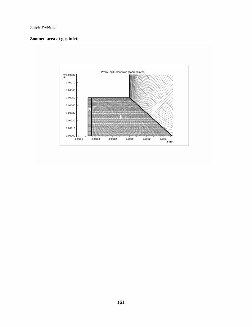
Sample Problems
Zoomed area at gas inlet:
-0.0006 -0.0004 -0.0002 0.0000 0.0002 0.00040.00000
0.00010
0.00020
0.00030
0.00040
0.00050
0.00060
0.00070
0.00080
z (m)
r (m
)
Prob7: NO Expansion (zoomed area)
1
2
3
161

Sample Problems
Comparisons to Data and Bird’s G2 DSMC Code
25 Torr Orifice Expansion - NO (Centerline)
Z / D
Rot
atio
nal T
emp
(K)
0 5 10 15 2050
75
100
125
150
175
200
225
250
Data - USAF Phillips Lab
Bartel DSMC-MP run 2
Campbell - Bird G2 code
25 Torr Orifice Expansion - NO (Z/D=3)
R / D
Rot
atio
nal T
emp
(K)
0 5 10 15 20 2570
80
90
100
110
120
130
140
150
Data - USAF Phillips Lab
Bartel DSMC-MP run 2
Bartel DSMC-MP run1
Campbell - Bird G2 code
TempleGraph 2.5, Origin: tjbarte@sass001 - Thu Jun 17 12:05:12 1993 (data file was DSMC-PV25T-XD3)
162
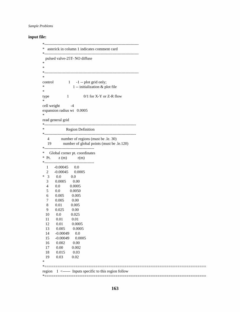
Sample Problems
input file:
*------------------------------------------------------------------------* asterick in column 1 indicates comment card*------------------------------------------------------------------------ pulsed valve-25T- NO diffuse***------------------------------------------------------------------------*control 1 -1 -- plot grid only;* 1 -- initialization & plot file*type 1 0/1 for X-Y or Z-R flow*cell weight -4expansion radius wt 0.0005*read general grid*----------------------------------------------------------------------* Region Definition*---------------------------------------------------------------------- 4 number of regions (must be .le. 30) 19 number of global points (must be .le.120)*--------------------------------------* Global corner pt. coordinates* Pt. z (m) r(m)*-------------------------------------- 1 -0.00045 0.0 2 -0.00045 0.0005* 3 0.0 0.0 3 0.0005 0.00 4 0.0 0.0005 5 0.0 0.0050 6 0.005 0.005 7 0.005 0.00 8 0.01 0.005 9 0.025 0.00 10 0.0 0.025 11 0.01 0.01 12 0.01 0.0005 13 0.005 0.0005 14 -0.00049 0.0 15 -0.00049 0.0005 16 0.002 0.00 17 0.00 0.002 18 0.015 0.03 19 0.03 0.02**=========================================================================region 1 <------ Inputs specific to this region follow*=========================================================================
163

Sample Problems
grid 14 global points coinciding w/ region corner points 1 - 4, resp. 15 2 1 30 number of cells along sides 1 and 3 50 number of cells along sides 2 and 4 0 sides 1 and 3 curvature: 0/1 for straight line/circular arc 0 sides 1 and 3 cell spacing: 3 1.03 50. sides 2 and 4 cell spacing: 1 boundary type code for sides 1 - 4, resp. 5 31 7 1 number of cells for which B.C.'s need to be read*-------------------------------------------------------------------------* Side Cell1 Cell2 elem/cell Spec. refl. Temp. K Material# Value*------------------------------------------------------------------------- 2 1 60 1 0.000 373. 0. 0.*-------------------------------------------------------------------------*-------------------------------------------------------------------------* Region interface/matching * Reg. side reg. sides Adj. side Adj. reg.*-------------------------------------------------------------------------*------------------------------------------------------------------------- 1 0 2 0 3 0 4 1 2 2 *=========================================================================region 2 <------ Inputs specific to this region follow*=========================================================================grid 1 global points 2 4 3 100 number of cells along sides 1 and 3 100 number of cells along sides 2 and 4 0 sides 1 and 3 curvature: 0/1 0 sides 1 and 3 cell spacing: 0 sides 2 and 4 cell spacing: 1 boundary type code for sides 1 - 4, resp. 7 5 7 1 number of cells for which B.C.'s need to be read*-------------------------------------------------------------------------* Side Cell1 Cell2 elem/cell Spec. refl. Temp. K Material# Value*------------------------------------------------------------------------- 3 1 100 1 0.000 373. 0. 0.
164

Sample Problems
*-------------------------------------------------------------------------*-------------------------------------------------------------------------* Region interface/matching * Reg. side reg. sides Adj. side Adj. reg.*-------------------------------------------------------------------------*------------------------------------------------------------------------- 1 0 2 1 4 1 3 0 4 1 1 3 *=========================================================================region 3 x <------ Inputs specific to this region follow*=========================================================================grid 4 global points 10 9 3 100 number of cells along sides 1 and 3 200 number of cells along sides 2 and 4 0 sides 1 and 3 curvature: 0/1 for straight line/circular arc 2 1.04 100. sides 1 and 3 cell spacing: 0 sides 2 and 4 cell spacing: 7 boundary type code for sides 1 - 4, resp. 5 7 1 1 number of cells for which B.C.'s need to be read*-------------------------------------------------------------------------* Side Cell1 Cell2 elem/cell Spec. refl. Temp. K Material# Value*------------------------------------------------------------------------- 2 1 200 1 0.000 373. 0.0 0.0*-------------------------------------------------------------------------*-------------------------------------------------------------------------* Region interface/matching data* Reg. side reg. sides Adj. side Adj. reg.*-------------------------------------------------------------------------*------------------------------------------------------------------------- 1 1 4 2 2 0 3 1 1 4 4 0*=========================================================================region 4 x <------ Inputs specific to this region follow*=========================================================================grid 10 global points 18 19 9 60 number of cells along sides 1 and 3
165

Sample Problems
40 number of cells along sides 2 and 4 0 sides 1 and 3 curvature: 0/1 for straight line/circular arc 0 sides 1 and 3 cell spacing: 2 1.02 10. sides 2 and 4 cell spacing: 7 boundary type code for sides 1 - 4, resp. 11 11 11 0 number of cells for which B.C.'s need to be read*-------------------------------------------------------------------------* Side Cell1 Cell2 elem/cell Spec. refl. Temp. K Material# Value*-------------------------------------------------------------------------*-------------------------------------------------------------------------*-------------------------------------------------------------------------* Region interface/matching data* Reg. side reg. sides Adj. side Adj. reg.*-------------------------------------------------------------------------*------------------------------------------------------------------------- 1 1 3 3 2 0 3 0 4 0*-------------------------------------------------------------------------END END OF EXPERT INPUT FILE*-------------------------------------------------------------------------
inlet file:
* freestream inlet condition for the ICF sphere* * Xe species*1 number of tables*0 ----- flag to specify freestream conditions3.216e20 400. 0.0 1500. 1500. 1500. 1.*
166

Sample Problems
species file:
**************************************** species data file ****************************************1 number of species*3 internal structure of most complex molecule:* 3-monatomic, 4-rotation, 5-rotat. + vibrat.*0 # of chemical reactions**-------------------------------------------------------------------------------------------------------------------* ID* Mwt Mol. mass Diam. #Rot.Deg. Rot.Rel. # Vib. Deg. Vib. Rel. Vib.Temp. specie wt. charge
omega tref alpha* (kg) (m) Freedom Coll. # Freedom Coll. # (K)*-------------------------------------------------------------------------------------------------------------------- Xe 131.229 2.18e-25 5.74e-10 0. 5. 0. 0. 0. 1.0 0.0 .85 300. 1.*END
167

Sample Problems
13.10 NO Vibrational Relaxation (Time Dependent)This problem is a transient simulation of the vibrational relaxation of NO where states V0, V1, and V2 are modelledusing a 6 reate equation model based on USAF Phillips Lab data. The simulation startes with a small amount(0.0001 mole fraction) of NO excited to V2 and V1 in a domain of V0. This simulations illustrates the trace speciesmodel in Icarus and the procedure to perform a transient simulation.- Input Gases: NO
- Surface Boundary Conditions:- 100% thermal accommodation- 100% specular surface reaction- Temperature of all surfaces = 300 K
- Gas Phase Chemistry:6 gas phase reactions (refer to chemistry file)
- Output:- pressure, velocity, temperature and species distribution- portray species weighting model- time accurate mole fractions
0.00000 0.00005 0.00010 0.00015 0.000200.00000
0.00002
0.00004
0.00006
0.00008
0.00010
0.00012
0.00014
Prob8: NO Vibration
z (m)
r (m
)
168

Sample Problems
input file:
-------------------------------------------------------------------------* asterick in column 1 indicates comment card*------------------------------------------------------------------------- 1 Region NO vib. relaxation 3 levels**-------------------------------------------------------------------------**control 1 -1 -- plot grid only;* 1 -- initialization & plot file*type 0 0/1 for X-Y or Z-R flow*read general grid*----------------------------------------------------------------------* Region Definition*---------------------------------------------------------------------- 1 number of regions (must be .le. 30) 4 number of global points (must be .le.120)*--------------------------------------* Global corner pt. coordinates* Pt. z (m) r(m)*--------------------------------------
NO - Vibrational Relaxation
time (microsec)
mol
e fr
actio
n
V1
V2
1001000
10000
0 25 50 75 100 125 1500.00
0.50
1.00
1.50
2.00
2.50
3.00x10⁻⁴
fit to data
DSMC - no wt. - 20,000/cell
DSMC - 100 - 2,800/cell
DSMC - 1000 - 2,500/cell
DSMC - 10000 - 1,700/cell
169

Sample Problems
1 0.000 0.000 2 0.000 1.0e-04 3 1.0e-04 1.0e-04 4 1.0e-04 0.000*------------------------------------------------------------------------* Individual Region Definitions Follow* --REGIONS NUMBERS MUST BE SEQUENTIAL--*------------------------------------------------------------------------*=========================================================================region 1 <------ Inputs specific to this region follow*=========================================================================grid 1 global points coinciding w/ region corner points 1 - 4, resp. 2 3 4 16 number of cells along sides 1 and 3 16 number of cells along sides 2 and 4 0 sides 1 and 3 curvature: 0/1 for straight line/circular arc 0 sides 1 and 3 cell spacing: 0 sides 2 and 4 cell spacing: 5 boundary type code for sides 1 - 4, resp. 5 5 5 4 number of bc entries*-------------------------------------------------------------------------* Side Cell Cell2 elem/cell Spec. refl. Temp. K Material # Value*------------------------------------------------------------------------- 1 1 16 1 1.000 300. 0 0. 2 1 16 1 1.000 300. 0 0. 3 1 16 1 1.000 300. 0 0. 4 1 16 1 1.000 300. 0 0.*-------------------------------------------------------------------------*-------------------------------------------------------------------------* Region interface/matching * Reg. side reg. sides Adj. side Adj. reg.*-------------------------------------------------------------------------*------------------------------------------------------------------------- 1 0 2 0 3 0 4 0*-------------------------------------------------------------------------END END OF EXPERT INPUT FILE*-------------------------------------------------------------------------
170

Sample Problems
inlet file:
** freestream inlet condition for NO relaxation* * NO: V0 V1 V2*1 number of tables*0 ----- flag to specify freestream conditions 3.296e22 0. 0.0 293. 93. 293. 0.9998 0.0001 0.0001*
species file:
**************************************** species data file ****************************************3 number of species*4 internal structure of most complex molecule:* 3-monatomic, 4-rotation, 5-rotat. + vibrat.*6 # of chemical reactions**-------------------------------------------------------------------------------------------------------------------* ID* Mwt Mol. mass Diam. #Rot.Deg. Rot.Rel. # Vib. Deg. Vib. Rel. Vib.Temp. specie wt. charge
omega tref alpha* (kg) (m) Freedom Coll. # Freedom Coll. # (K)*--------------------------------------------------------------------------------------------------------------------** this fit is for low temperature NO states; v0 30.0061 4.98E-26 4.26E-10 2. 1. 1. 1 0. 1.0 0. 0.9 300. 1.0v1 30.0061 4.98E-26 4.26E-10 2. 1. 1. 1. 0. 0.001 0. 0.9 300. 1.0v2 30.0061 4.98E-26 4.26E-10 2. 1. 1. 1. 0. 0.001 0. 0.9 300. 1.0*END
chemistry file:
*----------------------------------------------------------------------------* This input file contains the data characterizing the chemical reactions.**----------------------------------------------------------------------------* NO vibrational set 3 levelsV2 + V0 --> V1 + V1*0 3 1 1 1 2 2
171

Sample Problems
0. 5.559E-22 1.706E-19 0.5 -5.559E-22*V1 + V0 --> V2 + V0*0 2 1 1 1 3 10. 3.669E-20 8.885E-21 0.5 -3.669E-20*V0 + VO --> V1 + V0*0 1 1 1 1 2 10. 3.725E-20 4.442E-21 0.5 -3.725E-20*V1 + V1 --> V2 + V0*0 2 2 1 1 3 10. 0.00 1.706E-19 0.5 5.559E-22*V2 + V0 --> V1 + V0*0 3 1 1 1 2 10. 0.00 8.885E-21 0.5 3.669E-20*V1 + V0 --> V0 + V0*0 2 1 1 1 1 10. 0.00 4.442E-21 0.5 3.725E-20** third body probabilities now follow*0
Icarus input file:
# Test file for VIb -- 1000
log file dsmc.log
output screen 50
zero flag 50
random seed 3847
read def 1.0 dsmc.def
adapt flag 20000 0.25time factor 0.002
output special 400run 100000 0
172

Sample Problems
173

Sample Problems
13.11 Ion AcceleratorThis sample case has been included to demonstrate various input options for a complex chemically reacting plasmasimulation. However, this grid was generated in the early portion of the project and later grids were more efficientand easier to modify. The problem is axisymmetric with an ion source located near the centerline on the left side ofthe grid: ions and neutrals are injected here. The fine details of the ion generation are beyond the scope of physics inIcarus. The plume expands into the vacuum until it reaches the screen region of the ion extractor/accelerator. Here,the electrons are extracted to the grid and a large potential is applied to accelerate the ions to a target. One shouldcompare the gridding around the screen region in this problem with that in problem 13.5. Problem 13.5 wasgenerated using the multiple connected region capability of Icarus to drastically reduce the number of regions in thedomain and to greatly simplify the modification process.
The input files will not be reproduced here; they are available with the electronic form of this manual. This problemconsists of 49 regions; regions 1-5 are defined as ambipolar and with a Poisson solver used to determine the electro-static fields for the remainder. Ions and neutrals are injected in the ambipolar region and the expansion due both tothe simple half-spherical expansion and the ambipolar fields. When the ions enter the upstream region before thescreen, ’heavy’ electrons are injected as a rate to maintain quasi-neutrality in the initial cell. Now a Poisson solver isused to determine the electro-static fields. A ’heavy’ electron is defined as simply 1000 times the mass of anelectron (a pseudo-negative ion). The approximation gives up the accurate simulation of the sheaths at the screenfor an 20 - 50 time larger time step. Secondary electrons in the acceleration region are ’real’ electrons with theclassical electron mass.
Z
R
0 0.005 0.01 0.015 0.020
0.002
0.004
0.006
0.008
0.01
0.012
0.014
0.016
0.018
174

Sample Problems
Z
R
0.0035 0.004 0.0045
0.002
0.0025
0.003
0.0035
Z
R
0 0.001 0.002 0.003 0.004
0
0.002
0.004
175

Distribution
14.0 Distribution
External
E. Aydil Dept. Chemical & Nuclear Engr.University of California at Santa BarbaraSanta Barbara, CA 93106
A. BalakrishnaRTP DivisionApplied Materials2727 Augustine Drive, MS 0766Santa Clara, CA 95054
James BarryCreare Inc.PO Box 71Etna Rd.Hanover, NH 03755
Dave BraunLLNL MS L-0317000 East AvenueLivermore, CA 94550
I. BoydDepartment of Aerospace Engineering3012 FXB BuildingAnn Arbor, MI 48109-2140
T. S. CaleDept. Chemical & Material Engr.Arizona State UniversityTempe, AZ 8587
J. L. CecchiDept. Chemical and Nuclear Engr.209 Farris Engineering CenterUniversity of New MexicoAlbuquerque, NM 87131-1341
Gerald ChruscielOrg. L2-70; Bldg. 157Lockheed Martin Space Systems Corp.Missiles & Space OperationsPO Box 3504Sunnyvale, CA 94088-3504
Frank CollinsUniversity of Tenn. Space InstituteTullahoma, TN 37388
C.M.SurkoDepartment of PhysicsUniversity of California, San Diego9500 Gilman DriveLa Jolla, CA 92093-0319
D. EconomouDepartment of Chemical EngineeringUniversity of HoustonHouston, TX 77204-4792
Thomas R. FurlaniDepartment of ChemistryUniversity at BuffaloNSM ComplexBox 603000Buffalo, NY 14260-3000
Nick GatsonisRM 24-E104APL - Johns Hopkins UniversityJohns Hopkins RdLaurel, Md 20723
176

Distribution
D. B. GravesDepartment of Chemical EngineeringUniversity of California at BerkeleyBerkeley, CA 94720
James F. GrovesDirector, Research and Industrial ProgramsSchool of Engeering and Applied ScienceUniversity of VirginiaThornton Hall A127P.O. Box 400240Charlottesville, VA 22904-4240
M. J. HartigMotorolaMD: K-103501 Ed Bluestein BoulevardAustin, TX 78721
Derek HassSchool of Engeering and Applied ScienceUniversity of VirginiaThornton Hall A127P.O. Box 400240Charlottesville, VA 22904-4240
Bill HerlingBoeingMS 4C-619725 East Marginal Way S.Seattle, WA 98108
Chih-Ming HoDirector of Center for Micro SystemsMech., Aero, and Nuclear DepartmentUCLA405 Hilgard AvenueLos Angeles, CA 90024-1597
Charles JustizNASA Johnson Space CenterHouston, TX 77058
J. N. LevineAFRL/PRSA10 Saturn Blvd.Edwards AFB, CA 9324-7680
J. MossMS 408ANASA LangleyHampton, VA 23681
David W. PruittSverdrup Technology, Inc.939 Avenue CArnold AFB, TN 37389-9900
Y. RaWatkins-Johnson Company440 Kings Village RoadScotts Valley, CA 95066-4081
J. F. SantariusFusion Technology InstituteUniversity of Wisconsin-Madison1500 Engineering Dr.Madison, WI 53706
Vikram SinghNovellus Systems, Inc3970 North First StreetSan Jose, CA 95117
Chris SheltonMetal Matrix Composites - 3MBuilding 60-1N-01St. Paul, NM 55144-1000
Paul ShufflebothamNovellus Systems, Inc3970 North First StreetSan Jose, CA 95117
177

Distribution
C. ScottEG3NASA Johnson Space CenterHouston, TX 77058
Kenneth TatumSeverdrup Technology, Inc.740 Fourth St.Arnold Air Force Base, TN 37389-6001
V. Vahedilam research Corporation4650 Cushing ParkwayFremont, CA 94538-6470
P. A. VitelloMS L296Lawrence Livermore National LaboratoryP.O. Box 808Livermore, CA 94550
R. WalkerT-12, MS B268Los Alamos National LaboratoryLos Alamos, NM 87545
Y. YeApplied MaterialsMS 02253050 Bowers AvenueSanta Clara, CA 95054
Konrad ZhuRocketdyne Div.Rockwell International6633 Canoga Ave.Canoga Park, CA 91303
Sandia Internal
1 MS 1152 1642 M.L.Kiefer1 MS 1186 1674 T.A.Mehlhorn1 MS 0841 9100 T.C.Bickel1 MS 0834 9112 D.J.Rader1 MS 0826 9113 W. L. Hermina1 MS 0826 9113 C.C.Wong1 MS 0824 9115 J.L.Payne1 MS 0824 9115 C. Roy1 MS 0836 9117 M.A.Gallis1 MS 0321 9200 W. J. Camp1 MS 0310 9230 P. Yarrington1 MS 0820 9232 P.F.Chavez25 MS 0820 9232 T.J.Bartel1 MS 0316 9233 R.C.Schmidt1 MS 1111 9209 S.J.Plimpton1 MS 0828 9132 S.N.Burchett1 MS 1423 1118 M.Riley1 MS 1423 1118 P.Miller1 MS 1423 1118 J.Woodworth1 MS 0521 2502 F.M.Bacon1 MS 0516 2564 G.Laughlin1 MS 0516 2564 J.P.Brainard1 MS 0516 2564 C.N.Busick1 MS 0516 2564 R.J.Koss1 MS 1129 6428 D.L.Youchison
1 MS 9018 8945-1 Central Technical Files
2 MS 0899 9616 Technical Library1 MS 0612 9612 Review & Approval
For DOE/OSTI
178


![DSMC Moving-Boundary Algorithms for Simulating MEMS ......The Direct Simulation Monte Carlo (DSMC) method of Bird [14-15] is capable of simulating noncontinuum gas flows to high accuracy](https://img.pdfslide.net/doc/110x75/6123865e657f520df111905d/dsmc-moving-boundary-algorithms-for-simulating-mems-the-direct-simulation.jpg)
![Uncertainty quantification models for micro-scale squeeze-film … · 2013. 1. 30. · Monte Carlo (DSMC) [17] method for the solution of the Boltzmann equation is valid through](https://img.pdfslide.net/doc/110x75/5ff2de9e0def27133576003e/uncertainty-quantiication-models-for-micro-scale-squeeze-ilm-2013-1-30.jpg)


![Open Source DSMC Chemistry Modelling for Hypersonic Flows€¦ · undoubtedly the direct simulation Monte Carlo (DSMC) approach, originally proposed by Bird [7]. The DSMC technique](https://img.pdfslide.net/doc/110x75/60a259fb2563b9135324a098/open-source-dsmc-chemistry-modelling-for-hypersonic-flows-undoubtedly-the-direct.jpg)