Ice Bridge Level-1 Science Requirements and Scientific Basis

The IceBridge Science Team

March 6, 2011

1. IceBridge Program Overview and the IceBridge Science Team

NASA has established the Operation IceBridge program (OIB) which is mandated to fulfill the following observational goals:

P1 Make airborne altimetry measurements over the ice sheets and sea ice to extend and improve the record of observations begun by ICESat.

P2 Link the measurements made by historical airborne laser altimeters, ICESat, ICESat-2, and CryoSat-2 to allow accurate comparison and production of a long-term, ice altimetry record.

P3 Monitor key, rapidly changing areas of ice in the Arctic and Antarctic to maintain a long term observation record.

P4 Provide key observational data to improve our understanding of ice dynamics, and better constrain predictive models of sea level rise and sea ice cover conditions.

In additional, OIB has the following technical goal:

P5 Adapt existing instruments for airborne remote sensing of ice by unmanned aerial systems such as NASA’s Global Hawk.

The IceBridge Project is directed from NASA’s Goddard Space Flight Center. There are separate management functions for IceBridge Instruments, logistics, data management, and science. The 6 programmatic goals listed above provide general scientific direction for the project. Specific direction is provided by the IceBridge Science team (IST). The team has three tasks mandated by the Program (see OIB Science Team Terms of Reference Document, 2010):

Final development of the IceBridge Science Definition Document and Level-1 Scientific Requirements Document;

Evaluation of the IceBridge mission designs in achieving the goals defined by the Science Definition Document and Level-1 Scientific Requirements Document as requested by the NASA Program Scientist; and

Support to the IceBridge Program Scientist and Project Scientist in the development of the required analyses, documentation, and reporting during the IceBridge mission.

In addition, the science team, in collaboration with the instrument teams, will ensure the fidelity of the data products delivered to the public.  This includes thorough documentation and access to level 1 data and corrections (e.g. geophysical corrections, trajectory, orientation, ranging) so as

1

to provide a strong basis for future investigation and for improvement of the instrument level 2 products (e.g. footprint surface elevation).

This document addresses the first science team task to establish Level-1 science requirements. The science team adopted the following strategy for completing this task. First, the team articulated broad scientific goals or themes addressing Greenland and Antarctica ice sheets and sea ice and also glaciers in Alaska and ice caps in the Canadian Arctic. The goals then flowed into a set of more specific questions that could be addressed with the IceBridge data suite. The science questions were then linked to a set of observational goals, which are themselves driven by a set of specific measurement requirements. Science requirements (both measurement accuracy and geography requirements) are detailed in Section 5 of this report. Justification for many of the requirements parameters are reviewed in Section 6.

Note that the science themes, questions and measurement plans are important, ambitious and wide ranging. Consequently, the science community beyond just the IST is envisioned as active participants using the IceBridge data suite to address these questions. Two important functions of the IST are to engage the external community when developing data acquisition plans and to assure that the data set is as complete and as accurate as possible in order to facilitate broad and aggressive use by the science community. The team must walk the boundary between making recommendations on prudent and somewhat cautious use of the resources while at the same time anticipating the likelihood of new scientific investigations relying on a rich and cutting edge data set.

2. IceBridge Science Goals

At the highest level, the IceBridge data set will help address the following science goals (numerals in parentheses refer to Program Objectives of section 1.0).

Goal 1. Document volume changes over the accessible domain of the Greenland and Antarctica ice sheets between Icesat-1 and Icesat-2. A particular focus will be to document rapid changes. Icebridge will answer: how have the ice sheet volumes (areas accessible by a/c) changed during these 5 years? (P1,P2))

Goal 2. Document glacier ice thickness, basal characteristics and other geophysical properties to better interpret volume changes measured with laser altimetry and to enable more realistic simulations of ice sheet flow with numerical models. IceBridge will answer: how are the ice sheets likely to change in the future? (P3,P4)

Goal 3. Document the spatial and interannual changes in the mean sea ice thickness and the thickness distribution in the Arctic and Southern Oceans between ICESat-1 and ICESat-2, in support of climatological analyses and assessments.

Goal 4. Improve sea ice thickness retrieval algorithms by advancing technologies for measuring sea ice surface elevation, freeboard, and snow depth distributions on sea ice.

Note that IceBridge data cannot be used solely to tackle these important questions. Other data (for example, ice sheet surface velocity, sea ice deformation and motion data) must come from

2

other sources. However, IceBridge surface elevation, surface elevation change, and ice thickness data are essential ingredients needed to resolve these questions. Moreover, some of the measurements (swath altimetry and ice sounding radar) are only implementable on airborne platforms at present.

3. Science Questions

Several specific science questions flow from the IceBridge science goals. This increasing level science specificity will be used to establish quantitative measurement requirements. Shown in parentheses is the traceability from the science goal to each question.

Ice Sheets

IQ1. Where are glaciers continuing to thin and where may they be slowing/ thickening (G1)

IQ2. What are the major forces and mechanisms causing the ice sheets to lose mass and change velocity, and how are these processes changing over time? (G2) • How do the ice sheet/glacier surface topography, bed topography, bed geology,

ice shelves/tongues, and grounding line configurations effect ice dynamics?• How far inland are the effects of coastal thinning transmitted and by what

physical processes?• How far downstream do changing processes near the ice divide (changes in

snow accumulation, divide migration) effect glacier flow• What is the important scale for measuring geophysical parameters so as to

substantially improve modeling fidelity?• Where is the subglacial water produced and where is it going?

IQ3. How do ocean, sea ice, ice sheet interactions influence ice sheet behavior (G2)• How does the bathymetry beneath Arctic fjords and Antarctic ice shelves

influence ocean/ice sheet interactions and ice sheet/glacier flow dynamics?IQ4. What are yearly snow accumulation/melt rates over the ice sheets? (G1)

• How do changing accumulation rates (and hence near surface densities and firn structure) impact altimetry measurements

• What are the surface-melt flow-patterns and how do they change with time?

Sea Ice

SQ1. How are the physical characteristics of the sea ice covers changing (e.g. strength, thickness, snow depth, sea ice age)

SQ2. What level of accuracy in ice thickness observations is desirable for climate forecast? Operational forecast? for climate/operational?

SQ3. What is the optimal configuration of instruments to remotely measure:– Sea ice freeboard, as a function of sea ice elevation and sea surface elevation (via

leads)– Snow depth– Sea ice thickness (as derived from sea ice freeboard and snow depth)– Surface roughness (distinction of ice types, changes in ridge characteristics due

to ice dynamics, relating melt point coverage to snow depth)

3

– Change in floe size and lead width distribution (affects ice albedo feedback)SQ4. What is the optimal configuration of an Arctic sea ice observing network?

Antarctic?• How can data from in situ, airborne, submarine and satellite platforms, each with

a unique spatial and temporal signature, be effectively combined? • Are there locations that should be specifically monitored to aid in the observation

and prediction of ice volume (e.g. monitoring sea ice flux through Fram Strait)? SQ5. How does snow depth impact melt pond formation? What is the relationship

between between snow and ice roughness?SQ6. How is momentum being transferred between the ice and atmosphere? Ice and

ocean?

4. IceBridge Dataset Requirements

The IceBridge data set will have the following attributes based on the programmatic goals (section 1.0)

DR1. Provide a dataset for cross-calibration and validation of ice-sheet elevations from satellite lidars (ICESat-1, ICESat-2, DesDynI-Lidar) and radars (CryoSat-2 and Envisat). (P1,2,3)

DR2. Provide a dataset for improving and linking ICESat and ICESat-2 the ice-sheet elevation time series, including better characterization of ICESat-1 errors. (P1,2)

DR1. Provide a data sets for investigating critical ice sheet processes (P3,4)DR2. Provide a dataset for improving and comparing numerical models of ice-sheet

dynamics, especially precise maps of the bed beneath glaciers and coarse maps of the sea bed beneath ice shelves. (P3,4)

DR3. Provide a dataset for improving instrument simulation and performance analysis in support of future missions, such as ICESat-2 and DesDynI-Lidar. (P1,2)

DR4. Collaborate with field programs that will enhance interpretation of ice bridge data. (P4)

DR5. Provide a timely, well documented dataset for easy use by the science community. (P3,4)

DR6. The data set should complement the ongoing and planned programs of international partners (P2).

Programmatic goal P5 (UAV and advanced aircraft) does not trace into these data set requirements nor the baseline science requirements (section 5). However the issue of advanced systems and sensors is partly addressed in the projected science requirements.

5.0 IceBridge Science Requirements

As summarized in the body of the Project Plan, the IceBridge science requirements must satisfy NASA’s established programmatic goals to provide for measurement continuity between ICESat and ICESat-2, measurement comparison and continuity between ICESat/Cryosat-2/ICESat-2 to

4

create a decade long change record of ice sheet and sea ice characteristics, monitor rapidly changing areas of the arctic and Antarctic, improve understanding of ice dynamics, and to provide data necessary to improve predictive models. Specific science requirements (both measurement and geographic constraints are presented in this section. Measurement accuracy and geographic requirements are culled from the literature and are also based on the measurement parameter analyses presented in section 6.

Table W summarizes the threshold requirements that OIB must satisfy. The table combines both terrestrial and marine ice requirements and all have equal priority. Table X summarizes the prioritized baseline line science requirements that must be achieved by a multiyear, airborne measurement program designed to addresses the above objectives and reach the major scientific goals. To that end, the list is composed of relatively well established, essential parameters such as repeat measurement of ice surface topography, ice elevation change, ice thickness, glacier bed topography, snow thickness on sea ice, a first order description of bathymetry in front of tidewater glaciers and underneath ice shelves. There are also projected requirements in table Y that include a set of important parameters that could reasonably be sampled in the future but are not yet realized on an operational basis because of insufficient data to develop a vetted, standardized measurement methodology (for example, measuring the changing distribution of subglacial water; large scale measurements of surface accumulation rate; subglacial geothermal heat flux). Similarly, the science requirements include geographic objectives that are demonstrably in reach of manned aircraft in the time frames consistent with previous airborne programs in the polar regions. There are also spatial and temporal requirements that are highly desirable but which likely would require different platforms and operational strategies to achieve. Quoted measurement accuracies represent uncertainties of 1 standard deviation about the mean.

The science requirements also draw on publications that summarize community consensus on important variables and their measurement sensitivities (ISMASS, 2004; NRC, 2007, IGOS, 2007, ISMASS, 2010). The scientific basis for these requirements is presented in section 6.

Table W Operation IceBridge Threshold Science Requirements

T1. Measure annual changes in glacier, ice cap and ice sheet surface elevation sufficiently accurate to detect 0.15 m changes in uncrevassed and 1.0 m changes in crevassed regions along sampled profiles over distances of 500 m.

T2. Make sea ice surface elevation measurements with a shot-to-shot accuracy of 5 cm, assuming uncorrelated errors.

T3. Make sea ice elevation measurements of both the air-snow and the snow-ice interfaces to an uncertainty of 3 cm, which enable the determination of snow depth to an uncertainty of 5 cm.

T4. Acquire annually, near-contemporaneous, spatially coincident ice elevation data with ESA’s Cryosat for underpasses in the Arctic and Antarctica. Coordinate with ESA in situ validation campaigns as possible.

T5. Conduct one campaign in the Arctic and one campaign in the Antarctic each year

5

Table X Operation IceBridge Baseline Science Requirements

Table X.1 Baseline Science Requirements for Ice SheetsIS1. Measure surface elevation with a vertical accuracy of 0.5 m or better.IS2. Measure annual changes in ice sheet surface elevation sufficiently accurate to detect 0.15 m

changes in uncrevassed and 1.0 m changes in crevassed regions along sampled profiles over distances of 500 m.

IS3. Measure ice thickness with an accuracy of 50 m or 10% of the ice thickness, whichever is greater. IS4. Measure free air gravity anomalies to an accuracy of 0.5 mGal and at the shortest length scale

allowed by the aircraftIS5. Acquire annually, near-contemporaneous ice elevation data with ESA’s Cryosat for underpasses

across Greenland and Antarctica. Flight segment should span ESA SARIN and LRS mode boundaries. Coordinate with ESA in situ validation campaigns as possible.

IS6. Remeasure annually Antarctic and Greenland surface elevation along established airborne altimeter and ICESat underflight lines that extend from near the glacier margin to near the ice divide.

IS7. Collect elevation data so that the combined ICESAT-1-OIB sampling provides an elevation measurement within 10-km for 90% of the area within 100-km of the edge of the continuous Greenland Ice Sheet, as well the Antarctic Amundsen Sea Coast and Peninsula.

IS8. Measure ice thickness, gravity, surface, and bed elevation along central flowlines of the outlet glaciers in Greenland with terminus widths of 2 km or greater1. Measurements should extend at least 1.5 times farther than predicted outlet glacier valley dimensions. Repeat surface elevation measurements as practical.

IS9. Measure once, ice thickness, surface, and bed elevation across-flow transects at 3- and 8-km upstream of the terminus for each glacier in (8). Repeat surface elevation measurements as practical.

IS10. Measure once Greenland ice sheet elevation and ice thickness about four, nearly continuous close loops approximately about the 1000, 2000, and 2500 ice sheet elevation contours.

IS11. Measure ice thickness, elevation, gravity and magnetic anomalies over 10 Greenland glaciers2 and 15 Antarctic glaciers3 that are rapidly changing now or are likely to change in the next 10 years. Coverage should extend from the terminus to the elevation where velocities are about 50 m/yr. Over the fast flowing deep troughs, the grids must have 5-km spacing or better, with 10-km or better spacing on the surrounding regions of the lower catchment. Cycle through the glacier list for the duration of IceBridge.

IS12. Measure once ice thickness, surface elevation, gravity anomalies within 3 km of the Antarctic Ice Sheet Grounding line and along a second line located 10 km upstream of the grounding line.

IS13. Measure once surface elevation, ice thickness and seabed bathymetry beneath selected Antarctic Ice Shelves4, along Greenland Fjords5 where we will collect a line along the center of the fjords and three lines across (one at the sill, one near the middle, and one near the glacier front) and beneath Greenland Ice Tongues6.

IS14. Measure changing distribution of subglacial water over regions of rapidly flowing ice and distribution of subglacial water over interior cold ice.

IS15. Acquire submeter resolution, stereo color imagery covering laser altimetry swaths

6

Table X.2 Baseline Glaciers and Ice Caps RequirementIC1. Annually to semi-annually collect LiDAR swath data along the centerlines of major

Gulf of Alaska glacier and icefield systems, repeating previous IceSAT measurements and airborne laser altimetry centerline profiles7.

IC2. Make annual repeat measurement of surface elevation on select Alaskan GlaciersIC3. Make ice elevation, ice thickness and gravity measurements on Canadian Ice Caps at least twice

during the IceBridge program. Coverage should be based on previous airborne campaigns and leverage against ESA supported in situ Cryosat validation activities.

IC4. Make ice elevation, ice thickness and gravity measurements on selected ice caps and alpine glaciers around the Greenland Ice Sheet. Repeat the elevation measurements at least once during the IceBridge program8.

Table X.3 Baseline Requirement for Sea Ice SI1. Make surface elevation measurements with a shot-to-shot accuracy of 5 cm, assuming

uncorrelated errors.SI2. Make elevation measurements of both the air-snow and the snow-ice interfaces to an

uncertainty of 3 cm, which enable the determination of snow depth to an uncertainty of 5 cm. SI3. Provide annual acquisitions of sea ice surface elevation during the late winters of the

Arctic and Southern Oceans along near-exact repeat tracks, to within 500 m of the previous years’ flight tracks, in regions of the ice pack that are undergoing rapid change. Flight lines shall be designed to ensure measurements are acquired across a range of ice types including seasonal (first-year) and perennial (multiyear) sea ice to include, as a minimum: Arctic

a. At least two transects to capture the thickness gradient across the perennial and seasonal ice covers between Greenland, the central Arctic, and the Alaskan Coast.

b. Perennial sea ice pack from the coasts of Ellesmere Island and Greenland north to the pole, and westward across the northern Beaufort Sea.

c. Sea ice across the Fram Strait and Nares Strait flux gates.d. Sea ice covers of the Eastern Arctic North of the Fram Strait.

Antarctica. Weddell Sea ice between the tip of the Antarctic Peninsula and Cape Norvegia.b. Mixed ice cover in the western Weddell between the tip of Antarctic Peninsula and

Ronne Ice Shelf.c. The ice pack of the Bellingshausen and Amundsen Seas.

SI4. Include flight tracks for sampling the ground tracks of satellite lidars (ICESat-1 and ICESat-2) and radars (CryoSat-2 and Envisat) and, in the case of CryoSat-2, both IceBridge and CryoSat-2 ground tracks should be temporally and spatially coincident whenever possible. At least one ground track of each satellite should be sampled per campaign.

SI5. Conduct sea ice flights as early as possible in the flight sequence of each campaign, preferably prior to melt onset.

SI6. Collect coincident natural color visible imagery of sea ice conditions at a spatial resolution of at least 20 cm per pixel to enable direct interpretation of the altimetric data.

SI7. Conduct sea ice flights primarily in cloud-free conditions, and data shall be retained

7

under all atmospheric conditions, such that a flag shall be included to indicate degradation or loss of data due to clouds.

SI8. Make full gravity vector measurements on all low-elevation (< 1000 m) flights over sea ice, to enable the determination of short wavelength (order 10 to 100 km) geoid fluctuations along the flight track to a precision of 2 cm.

SI9. Actively seek out and coordinate with field campaigns that are consistent with and advance IceBridge project objectives to extend and improve the record of observations begun by ICESat related to sea ice thickness and snow depth retrievals.

SI10. Make available to the community instrument data on sea ice surface elevation and snow depth within 3 months of acquisition, and derived products (via NSIDC) within 6 months of data acquisition.

Table Y Projected Science Requirements on Future IceBridge Development

Table Y.1 Projected Ice Sheet Science Requirements on Future IceBridge Development1. Measure surface snow accumulation rate with an accuracy of 4 cm/yr averaged over 25 km square

areas in dry snow regions with annual accumulation in excess of 10 cm/yr. 2. Measure the distribution and changing distribution of subglacial water over 5 km square areas.3. Seasonally remeasure surface elevation on select Greenland and Antarctic Glaciers using UAVs.4. Estimate relative spatial changes in subglacial geothermal heat flux using ice thickness, gravity and

magnetic data.5. Remeasure ice sheet surface elevation at the locations of ICESat detected subglaical lakes located

beneath West Antarctic Ice Streams and outlet glaciers draining into the Ross Ice Shelf. Measure with accuracy of 10 cm and at least once during the IceBridge mission using UAVs.

6. Measure free air gravity anomalies to an accuracy of 0.5 mGal and a wavelength of 2.5km7. Acquire photogrammetrically calibrated, stereo, color imagery covering laser altimetry

swaths and adjacent areas for creating DEMs and orthophotographs with submeter resolution and accuracy.

8

Table Y.2 Projected Sea Ice Science Requirements on Future IceBridge Development 1. Improve sea ice baseline requirement 1 to make surface elevation measurements with a shot-

to-shot accuracy of 3 cm (versus 5 cm), assuming uncorrelated errors. 2. Extend sea ice baseline requirement 3 to other regions of the Arctic and Southern Oceans:

Arctic(to better constrain estimates of sea ice volume change)a. North Pole regionb. Southern Beaufort Sea, west of Banks Islandc. Sea ice along the east coast of Greenlandd. Southern Chukchi Sea north of Bering Straite. Davis Straitf. Lancaster Sound and other parts of the Canadian Archipelago

Antarctic(to better understand the process of sea ice formation and snow accumulation)a. Ross Sea b. Surveys of areas of polynya formation, over and downwind of the polynya c. Surveys of areas where katabatic winds may deposit abundant snow.

3. Collection thermal images for a swath that, as a minimum, covers the LVIS data swath with a resolution of 0.5 m or better, and are calibrated to brightness temperature with an accuracy of 0.1K.

4. Improve sea ice baseline requirement 6 to collect coincident digital stereo imagery of sea ice conditions at a spatial resolution of at least 10 cm (versus 20 cm) per pixel, at a vertical resolution of 20 cm, to enable direct interpretation of the altimetric data and provide a complimentary surface elevation product.

5. IceBridge shall support the validation of operational sea ice analysis and forecast products by providing estimates of sea ice freeboard within 1 week of data acquisition, and estimates of sea ice thickness within 2 weeks of data acquisition.

Footnotes on the Requirements1. For a list of Greenland outlet glaciers see Moon and Joughin (2007)2. The targeted list of Greenland glaciers includes but is not exclusive to: Petermann, Humboldt, 79 North, Zaceriea (NE IceStream), Store, Rinks, Jacobshavn, Eqalorutsit kangigdlit sermiat, Nordboggletscher, Helheim, Daugaard-Jensen3. The list of Antarctic Glaciers includes but is not exclusive to: Pine Island, Thwaite, Crane, Rutford, Lambert, Toten, Mertz, Shirase, Recovery, Jutulstraumen, David, Byrd, Nimrod, WAIS Ice Streams.4. The list of ice shelves includes but is not exclusive to: Getz, Dotson, Crosson, Thwaites, Pig, Cosgrove, Abbot, George VI, Larsen C, Venable, Cook, Moscow, Totten, Riiser Larsen, Fimbul, West, Shackleton.5. The list of fjords includes but is not exclusive to: Nordre Sermilik, Kangiata (Nuuk), jakobshavn, Torssukataq, Ummanaq (3 fjords), Upernavik, and the mini fjords in Melville bay should be pursued based on the 2010 results, Ingelfield Bredening (north thule) and Humboldt Heimdal Fj., Bernstorft Fj., Gylden love fj., Helheim, Kangerlugssuaq, Vestfjord, Daugaard Jensen, Keyser Franz Joseph Fj., Borfjorden (Storstrommen). 6. The list of ice tongues includes but is not exclusive to: Peterman, 79 north, and Zacheriae Glaciers.7. Targeted glaciers include but ar not exclusive to the Columbia-Tazlina system, the Bering-Bagley system, the Seward-Malaspina system, the Yathse, Guyot, Tyndall and Tsaa tidewater glaciers in Icy Bay,

9

the Yakutat Icefield, Glacier Bay's Grand Plateau, Fairweather, Grand Pacific, Margerie, Brady, Carroll, and Muir glaciers, and finally the Stikine, Juneau, Nabesna and Harding Icefields.8. Coverage will be selected to be representative for varying climate zones and priority will be given to ice caps and alpine adjacent to rapidly changing ice sheet regions. Suggested regions: Sukkertoppen Iskappe, Disko Island, North Ice Cap, Kronprins Christian Land, Renland Iskappe.

6. Scientific Basis for IceBridge Science Requirements

The purpose of this section is to establish the science basis for IceBridge baseline requirements on ice sheet, glacier, and sea ice measurements. Other useful tabulations of cyrospheric measurement requirements can be found in the literature (e.g. IGOS, 2007; ISMASS, 2004, 2010) and we have relied on the literature to further support our requirement specifications. We do not separately address the threshold requirements as these constitute the essential subset of the baseline requirements.

6.1. Ice Sheets, Ice Caps, Glaciers Baseline Justification

(IS1) Elevation requirements are estimated based on ice sheet driving stress (d)

τ d=ρgH ∂ h∂ x

Here, is the density, g is acceleration due to gravity, H is the ice thickness and h is the surface topography. Driving stress on West Antarctic Ice streams is approximately 10 kPa. Using that number as a required measurement accuracy, and selecting 1000 m of ice as a reasonable average value, the required accuracy on driving stress is written as

∆ τd=10 kPa={( ρgH (∆ ∂ h∂ x ))

2

+( ρg ∂ h∂ x

(∆ H ))2}

1 /2

Assuming the total driving stress uncertainty is distributed equally between the two terms, the required surface slope accuracy is 0.06 degrees. Taking the surface slope (S) as

S= ∂h∂ x

=h0−h1

xo−x1

and assuming negligible error in the longitudinal coordinate, the uncertainty in S is

∆ S=√2∗∆ hxo−x1

From here we can estimate either the requirement on surface elevation accuracy or the required sample spacing. For the 0.06 degree slope accuracy requirements and choosing the instrumental surface elevation error to be 0.5 m, the required surface elevation sample spacing is about 700 m (or about an ice thickness for this case) in the along flow direction. Alternatively, the sample

10

spacing could be chosen and the elevation accuracy estimated. So if we set the sample interval at 1 km, the requirement on elevation accuracy is 0.75 m. We retain the 0.5 m requirement based on the IGOS recommendation of 0.5 m at 1 km sampling intervals (IGOS, 2007, p. 86).

IS2) Ice elevation change requirements follow from an assessment of natural variabilities separate form average annual mass loss, which occurs on scales of months to years with magnitudes of cm/yr to ~10 m/yr. The near surface density changes with temperature, accumulation rate and month (equivalent seasonal changes in surface elevation are on the order of 20 cm). The net surface accumulation can change daily. The surface roughness can change diurnally. Surface roughness influences the instantaneous mean-elevation accuracy of a small area (over an instrument footprint where roughness is typically 5-10 cm rms on the interior ice sheet). For these reason, local surface elevation change knowledge is required to about 15 cm. To further refine our estimates of surface elevation change, we require having many, near simultaneous, independent observations to remove natural random fluctuations. A meaningful spatial averaging dimension of independent observations depends on the terrain but is between 1 and 5 km sq areas for the perimeter areas.

The requirements on spatial repeatability accuracy are as follows. For regions where 2-dimensional data are acquired (1x1 km), the exact distribution of independent samples within the area is not important. For places where we simply have at least 500 m long tracks of narrow swaths (ATM for example), we need to have the swaths overlap to say 50% in order to reduce slope induced errors. ATM has achieved this overlap goal.

IS3) The depth integrated continuity equation informs on the required ice thickness requirements. Writing the equation as a spatially averaged volume-balance over an area A that extends from near the grounding line of a basin to the bounding ice divides, the spatially averaged change in ice thickness, H, (or elevation h on a static crust) is expressed in terms of the output Qo flux, the basin averaged accumulation rate a and the basin averaged basal melt rate b

dhdt

=−(Qo)

A+ a+b (1)

The flux across an output gate is given asQo=α VH S

Here V is the speed orthogonal across the outward boundary S of the basin. Vertical variation in the speed is accounted for by a weighting parameter .

Assuming the errors on each measurement parameter are normally distributed, the variance of the flux is

(δ Qo )2=(αVSδH )2+ (αHXδV )2++(αHVδS )2+ (HVSδα )2(2)

Accounting for errors in the interface balance terms, the error on the equivalent, basin-averaged thickening rate is

δ dhdt

=¿¿

11

The equation illustrates that there are 7 distinct error terms contributing to the error in ice sheet thickening rate. Taking the error on elevation changes as 15 cm/yr and given that the length of the outflux gate S, the depth-averaged-velocity tuning parameter (), and the velocity V, and the basin area A can be accurately measured or reasonably modeled, the allowable error on the remaining terms probably can be relaxed to (15/(3)1/2) cm/yr or about 9 cm/yr ice equivalent. This now allows an estimate on the required thickness accuracy from

(9 cm / yr )2=(αVSδHA )

2

Taking V to be 1000 m/yr, S to be 1200 km, is unity, and A is 10^6 km (roughly the dimensions of the Amery drainage and around the grounding line) the average error in ice thickness needs to be about 75 m. Given that this is one of if not the largest glacier drainage in the world, it seems reasonable to reduce the ice thickness error to 50 m on average for a basin half this size.

Ice sounding radars are capable of achieving these levels of accuracy as illustrated by following Skolnick (1962, p 464) who adopts the following relations for estimating travel time accuracy on radar measurements in the presence of noise

∆ T=tr

( SN )

Here T is the echo arrival time uncertainty, tr is the echo rise time, S is the signal strength and N is the noise (clutter) level. Conservatively taking the rise time as proportional to the inverse bandwidth (bw)

∆ T=( 1bw )( SN )

And the ice thickness error is

∆¿ V2

∆ T=V2

( 1bw )( S

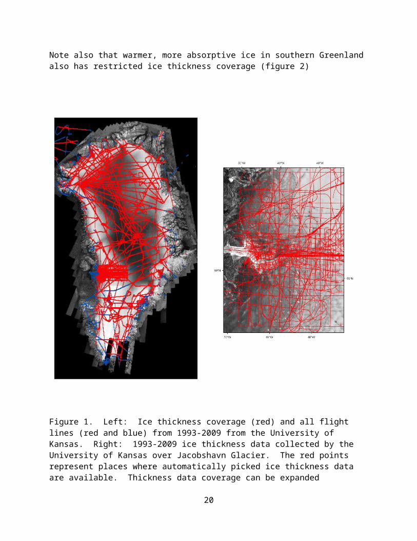
N )UHF and VHF radars are presently operating at bandwidths of about 20 MHz. For 0 dB SNR, the echo time error results in about 4 m error in ice thickness. Allowing for small errors in wave speed (well documented in both the laboratory and in the field), an ice thickness uncertainty of 50 m is well realizable with existing radar systems. The two confounding factors which reduce SNR are surface clutter and temperature-dependent absorption. Both processes are important in fast flowing outlet glaciers. This is illustrated in the coverage map showing where ice thickness data have been successfully acquired by the University of Kansas (Figure 1 ). Consequently we impose a less restrictive requirement of 10% of the ice thickness for outlet glaciers. Note also

12

that warmer, more absorptive ice in southern Greenland also has restricted ice thickness coverage (figure 2)

Figure 1. Left: Ice thickness coverage (red) and all flight lines (red and blue) from 1993-2009 from the University of Kansas. Right: 1993-2009 ice thickness data collected by the University of Kansas over Jacobshavn Glacier. The red points represent places where automatically picked ice thickness data are available.  Thickness data coverage can be expanded (especially along the length of the glacier channel) by using advanced signal processing to enhance bed echoes and manual picking techniques, as has been demonstrated on other glaciers . Consequently, these maps are a conservative estimate of coverage. (Figure compiled by A. Hock and K. Jezek)

13

Figure 2. Basal topography and ice thickness data coverage (IS4). Figure prepared by E. Rignot.

IS4) Gravity Measurement Accuracy. Gravity measurements are key to constraining ice sheet/glacier bed topography, grounding line configurations, bathymetry beneath ice shelves and ice tongues, fjord geometry and bed geology which can inform about basal conditions. Each of these parameters acutely impacts ice dynamics. Gravity data are essential to constrain bathymetry beneath ice shelves, floating ice tongues as well as the geometry of ice covered fjords inaccessible to classic surface ship marine geophysical measurements. Gravity can be used to identify sills in front of major outlet glaciers that will influence the transfer of warm marine water towards grounding lines. Oceanographic studies require topographic estimates +/- 50m to constrain the nature of the ocean-ice interaction. Finally gravity can be used to constrain the nature of the bed beneath ice sheets, outlet glaciers and ice streams. Regions of soft and hard bed can be linked to the underlying bedrock geology. Identifying the presence of any subglacial sediments or till beneath regions of fast flowing ice has the potential to improve ice sheet models.

In optimal conditions, airborne gravity measurements are capable of providing topographic estimates that are accurate to better than 50m. In the ideal world, airborne gravity measurements

14

accurate to .5 mGal would produce a topographic model accurate to ~7.5m. Topographic and bathymetric models derived from gravity are limited by geologic “noise” or density variations within the regional topography and the fundamental resolution limitation associated with making measurements from a moving platform. As airborne gravity data requires a time-based filter, faster aircraft speeds result in decreased spatial resolution. Geologic “noise” can be reduced by linking bathymetric models to known geologic structures or by use of complimentary data sets such as magnetics. In Greenland and Antarctica, magnetic data can be used to help constrain subice geology along with the gravity data. For example, where the gravity data detects a ridge in the basement, the magnetic data can be used to differentiate between glacial till and crystalline basement for the ridge composition. An airborne magnetic system can image sub-ice geology such as volcanic rocks, crystalline basement and sedimentary basins.

Documenting the movement of water beneath the large ice shelves is key to understanding ocean-ice interactions but requires an accurate knowledge of the ice shelf cavity. Cavity geometry has been very difficult to obtain. Both the ice shelf thickness and the bathymetry of the continental margin are necessary to define the cavity geometry. Radar can measure the upper surface of the cavity but does not penetrate the water underneath. Exploration with autonomous underwater vehicles is possible but provides relatively little spatial coverage. Airborne gravity can support new bathymetric models beneath ice shelves. Examples of targets for recovering ice shelf bathymetry include the Petermann Glacier in Greenland and the Larsen C, Getz, Abbott and King George V ice shelves in Antarctica. An orthogonal grid of flight lines acquired at 5-10 km line spacing is appropriate to provide a regional bathymetry model. Over Larsen C a 20-50 km spaced airborne grid provides preliminary insights into the broad regional bathymetric trends, specifically overdeepenings adjacent to the grounding line and cross shelf troughs. (Cochran and Bell 2011).

Sill geometry is important as these ridges of elevated topography can provide pinning points for ice shelves or ice tongues or alternatively serve as a basic barrier to the flux of water between the global ocean to the ice sheet grounding line. 40 km in front of Thwaites Glacier a prominent ridge or sill serves as a pinning point for the remaining ice tongue. The sills in front of Thwaites and Pine Island Glaciers in Antarctica as well as 70-550m sills in front of many Greenland fjords are a basic valve on the circulation of ocean water to the grounding line. Estimating sill depths from gravity is best based on profiles perpendicular to the sill, generally profiles along the fjord, orthogonal to the grounding line. For the optimal bathymetric solutions 5 km line spacing orthogonal to the targeted sill and with cross lines is the best survey design.

Basal conditions are key to understanding the evolution of ice sheet velocity. Identification of sedimentary basins in West Antarctica have been aligned to the onset of fast flow of the ice streams (Bell et al, 1998, Anandakrishnan et al, 1998). Gravity can be used to identify the presence of sediments and hence the presence of a soft bed. The trough beneath Jakobshaven is filled by over 1 km of sediments based on the gravity data acquired from a Twin Otter (Block and Bell, 2010).

Gravity data collected as part of OIB have been demonstrated to achieve repeatabilities and accuracies better than several tenths of a milligal, which is an extraordinary accomplishment (see http://bprc.osu.edu/rsl/IST/documents/IceBridge%20AIRGrav%20Accuracy.pdf). High accuracies where achieved over long, straight, low elevation flights over sea ice and the Sanders result was independently confirmed by the IST. Over ice sheets, we expect that the instrument accuracy is similar but complications from geophysical structures can degrade repeatability. In

15

the Sanders report quoted above, cross over difference standard deviations are about 1.5 milligal for filter lengths of about 83 sec. Accuracies degrade for both longer and shorter filters. Independent analysis by the IST generally confirms the ice sheet result. As noted above, we can use a simple Bouguer slab analysis to estimate that a 2 milligal uncertainty roughly equates to a 50 m uncertainty in the thickness of a water slab (density contrast 1 gm/cc).

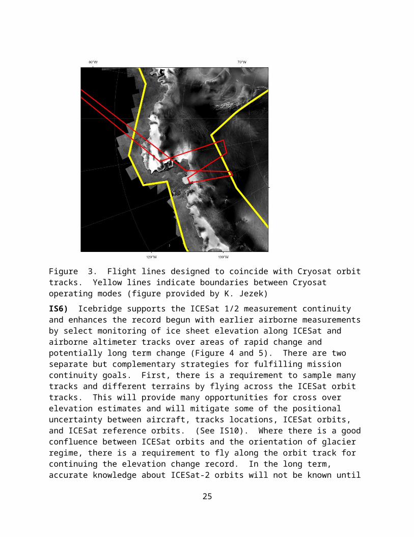
IS5) Near contemporaneous ice elevation data should be acquired during overflights of Cryosat-2. The primary goal of the data acquisitions is to intercompare laser and radar altimeter data and to improve the ice elevation change record that will eventually span ICESat-1 to Cryosat-2 to ICESat-2. At least one OIB ice sheet underflight should occur during each Arctic and Antarctic deployment. The underflights should span a distance starting seaward of the ice sheet when Cryosat-2 is operated in the SARIn mode. The underflight should continue at least 100 km past the point at which the satellite is operating in low-resolution mode. Locations selected for underflights should maximize the range of ice sheet surface slopes and glacier regimes to facilitate the best comparison of lidars and Cryosat radars for later, long term development of elevation change records. Figure is an example of a Cryosat underflight across the complex topography of Pine Island and Thwaites Glaciers and illustrates the boundaries between Cryosat operating modes.

Figure 3. Flight lines designed to coincide with Cryosat orbit tracks. Yellow lines indicate boundaries between Cryosat operating modes (figure provided by K. Jezek)

IS6) Icebridge supports the ICESat 1/2 measurement continuity and enhances the record begun with earlier airborne measurements by select monitoring of ice sheet elevation along ICESat and

16

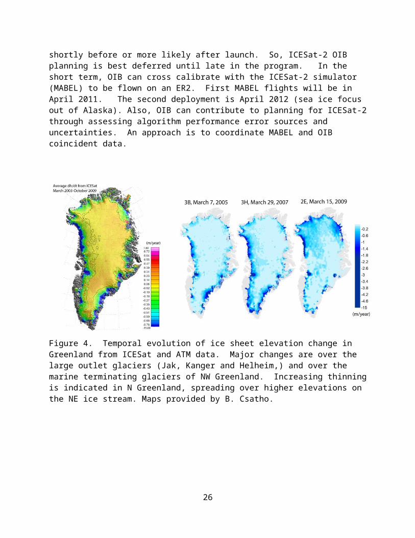
airborne altimeter tracks over areas of rapid change and potentially long term change (Figure 4 and 5). There are two separate but complementary strategies for fulfilling mission continuity goals. First, there is a requirement to sample many tracks and different terrains by flying across the ICESat orbit tracks. This will provide many opportunities for cross over elevation estimates and will mitigate some of the positional uncertainty between aircraft, tracks locations, ICESat orbits, and ICESat reference orbits. (See IS10). Where there is a good confluence between ICESat orbits and the orientation of glacier regime, there is a requirement to fly along the orbit track for continuing the elevation change record. In the long term, accurate knowledge about ICESat-2 orbits will not be known until shortly before or more likely after launch. So, ICESat-2 OIB planning is best deferred until late in the program. In the short term, OIB can cross calibrate with the ICESat-2 simulator (MABEL) to be flown on an ER2. First MABEL flights will be in April 2011. The second deployment is April 2012 (sea ice focus out of Alaska). Also, OIB can contribute to planning for ICESat-2 through assessing algorithm performance error sources and uncertainties. An approach is to coordinate MABEL and OIB coincident data.

Figure 4. Temporal evolution of ice sheet elevation change in Greenland from ICESat and ATM data. Major changes are over the large outlet glaciers (Jak, Kanger and Helheim,) and over the marine terminating glaciers of NW Greenland. Increasing thinning is indicated in N Greenland, spreading over higher elevations on the NE ice stream. Maps provided by B. Csatho.

17

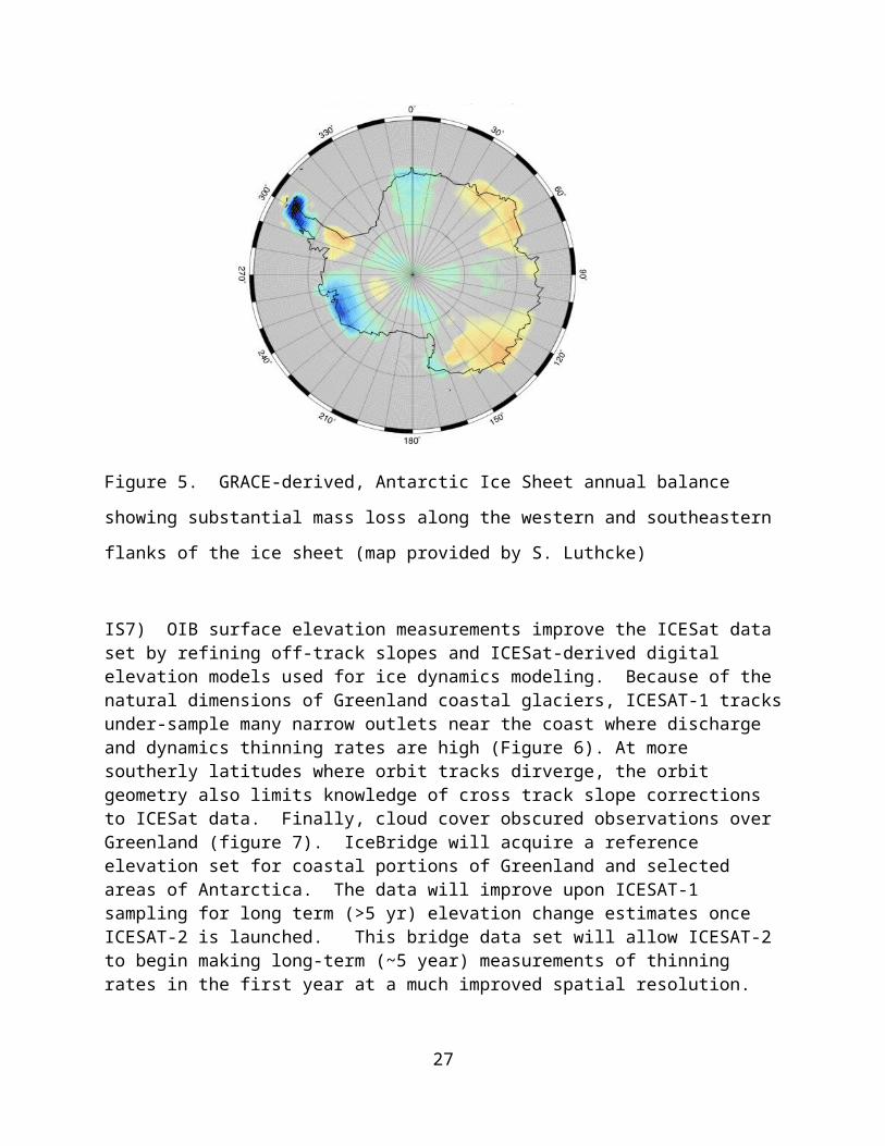
Figure 5. GRACE-derived, Antarctic Ice Sheet annual balance showing substantial mass loss

along the western and southeastern flanks of the ice sheet (map provided by S. Luthcke)

IS7) OIB surface elevation measurements improve the ICESat data set by refining off-track slopes and ICESat-derived digital elevation models used for ice dynamics modeling. Because of the natural dimensions of Greenland coastal glaciers, ICESAT-1 tracks under-sample many narrow outlets near the coast where discharge and dynamics thinning rates are high (Figure 6). At more southerly latitudes where orbit tracks dirverge, the orbit geometry also limits knowledge of cross track slope corrections to ICESat data. Finally, cloud cover obscured observations over Greenland (figure 7). IceBridge will acquire a reference elevation set for coastal portions of Greenland and selected areas of Antarctica. The data will improve upon ICESAT-1 sampling for long term (>5 yr) elevation change estimates once ICESAT-2 is launched. This bridge data set will allow ICESAT-2 to begin making long-term (~5 year) measurements of thinning rates in the first year at a much improved spatial resolution.

18

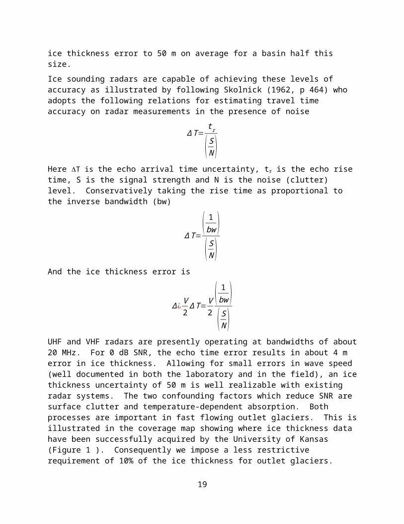
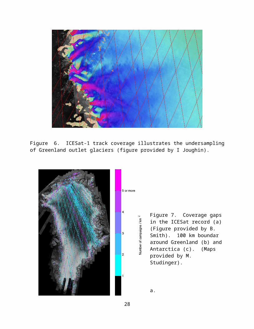
Figure 6. ICESat-1 track coverage illustrates the undersampling of Greenland outlet glaciers (figure provided by I Joughin).

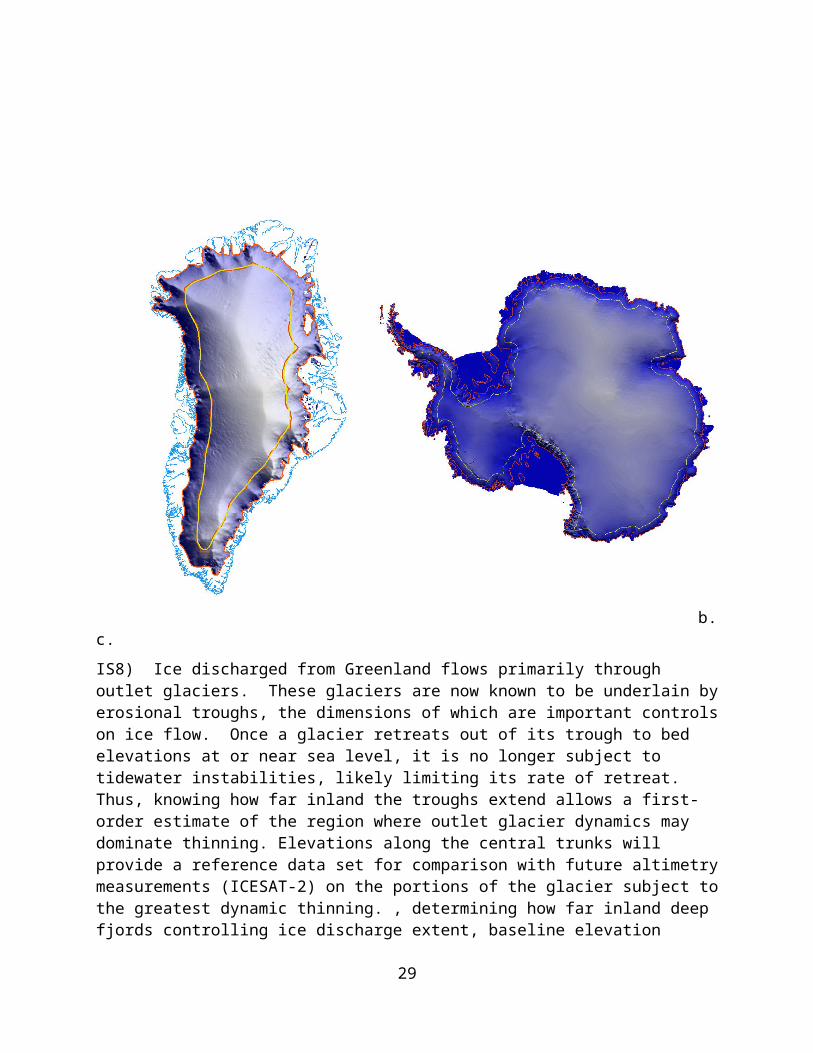
Figure 7. Coverage gaps in the ICESat record (a) (Figure provided by B. Smith). 100 km boundar around Greenland (b) and Antarctica (c). (Maps provided by M. Studinger).

a.

19

b. c.

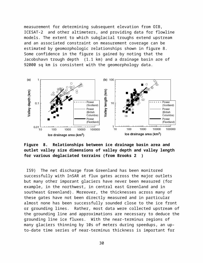
IS8) Ice discharged from Greenland flows primarily through outlet glaciers. These glaciers are now known to be underlain by erosional troughs, the dimensions of which are important controls on ice flow. Once a glacier retreats out of its trough to bed elevations at or near sea level, it is no longer subject to tidewater instabilities, likely limiting its rate of retreat. Thus, knowing how far inland the troughs extend allows a first-order estimate of the region where outlet glacier dynamics may dominate thinning. Elevations along the central trunks will provide a reference data set for comparison with future altimetry measurements (ICESAT-2) on the portions of the glacier subject to the greatest dynamic thinning. , determining how far inland deep fjords controlling ice discharge extent, baseline elevation measurement for determining subsequent elevation from OIB, ICESAT-2 and other altimeters, and providing data for flowline models. The extent to which subglacial troughs extend upstream and an associated constraint on measurement coverage can be estimated by geomorphologic relationships shown in figure 8. Some confidence in the figure is gained by noting that the Jacobshavn trough depth (1.1 km) and a drainage basin are of 92000 sq km is consistent with the geomorphology data.

20

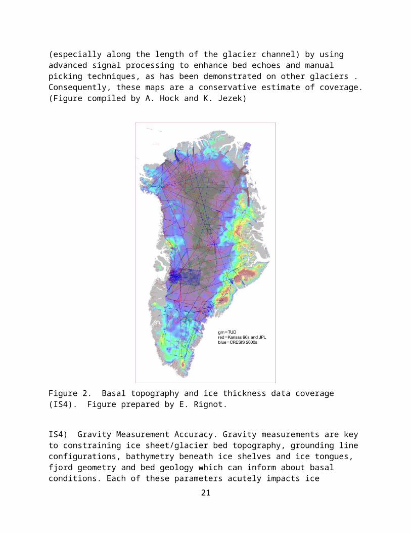
Figure 8. Relationships between ice drainage basin area and outlet valley size dimensions of valley depth and valley length for various deglaciated terrains (from Brooks 2 )

IS9)  The net discharge from Greenland has been monitored successfully with InSAR at flux gates across the major outlets but many other imporant glaciers have never been measured (for example, in the northwest, in central east Greenland and in southeast Greenland). Moreover, the thicknesses across many of these gates have not been directly measured and in particular almost none has been successfully sounded close to the ice front or grounding lines. Rather, most data were collected upstream of the grounding line and approximations are necessary to deduce the grounding line ice fluxes. With the near-terminus regions of many glaciers thinning by 10s of meters during speedups, an up-to-date time series of near-terminus thickness is important for tracking ice discharge variability, particularly as missions such as DESDynI provide more frequent velocity mapping.

To obtain a complete and comprehensive estimation of ice fluxes into the ocean, not only for mass balance purposes but also for freshwater fluxes into the ocean, OIB will strive to collect ice thickness measurements as close as possible to the glacier grounding lines. Cross flow profiles and along flow profiles will be necessary to evaluate the precision of the mapping and reduce residual uncertainties. A one-time OIB radar sounding mapping to determine the bedrock depths will allow thickness to be tracked through time with subsequent altimeter-only surface mappings (i.e., OIB, ICESAT-2, and DESynI). With this objective in mind, OIB will measure thickness at gates located 3 and 8-km from the present termini of the ~200 outlet glacier in Greenland with widths of 2-km or more. The 3-km flux gates will provide the thicknesses necessary for a comprehensive determination of the ice flux discharge from Greenland. The 8-km gate will provide a second gate for instances where the terminus retreats by more than 3-km. In addition to providing flux gates, these transects along with the along-flow transects (IS8) will provide at least some bed elevation/thickness information for ice sheet modeling of all major glaciers.

In addition, OIB will document ice fluxes farther upstream as this will enable the determination of the pattern of net mass balance of the glacier farther upstream, and will enable the determination of future ice fluxes when glaciers retreat farther inland.

21

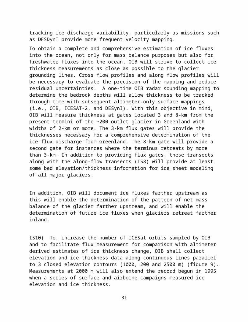
IS10) To, increase the number of ICESat orbits sampled by OIB and to facilitate flux measurement for comparison with altimeter derived estimates of ice thickness change, OIB shall collect elevation and ice thickness data along continuous lines parallel to 3 closed elevation contours (1000, 200 and 2500 m) (figure 9). Measurements at 2000 m will also extend the record begun in 1995 when a series of surface and airborne campaigns measured ice elevation and ice thickness.

B

Figure 9. 1000, 2000 and 2500 m contours about the Greenland Ice Sheet (left). Contours in the vicinity of Jacobshavn Glacier and ICESat reference orbits (right).

IS11) . The inability to place an upper bound on sea level change in the last IPCC reports stems largely from the uncertainty in our knowledge of glacier dynamics, the physics of which are not included in current whole ice-sheet models. OIB will acquire a comprehensive set of measurements for process modeling studies aimed at understanding outlet glacier dynamics. The data set will allow the development of process-level model experiments to determine the physics that govern fast flow and to develop the parameterizations needed for larger-scale predictive models. A representative set of glaciers should be chosen, including Jakobshavn, Kanger, Helheim, a northern glacier, and 2 or 3 glaciers each from the currently changing regions in the northwest and southeast. Measurements will extend to interior regions where surface velocities decrease to 50 m/yr (Figure 10). Coverage requirements are justified in the following sections.

22

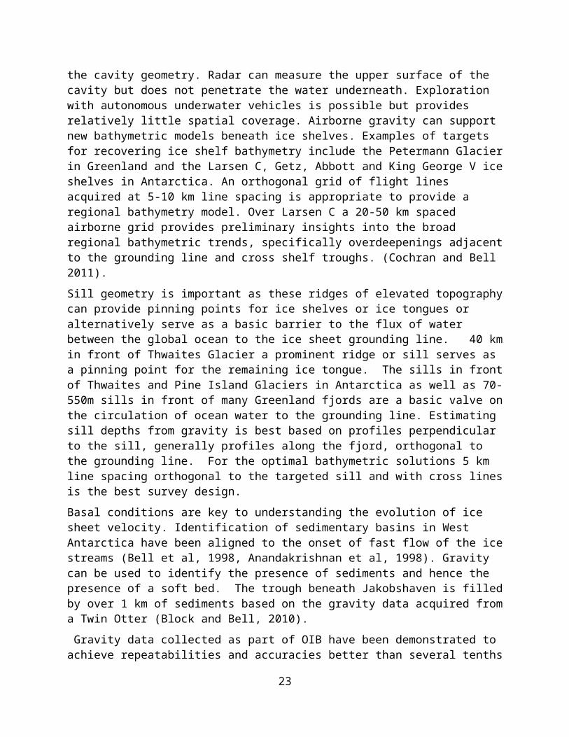
Figure 10. Surface velocity thresholds on the Greenland Ice Sheet. (Figure provided by E. Rignot).

Detailed bed mapping in selected region.

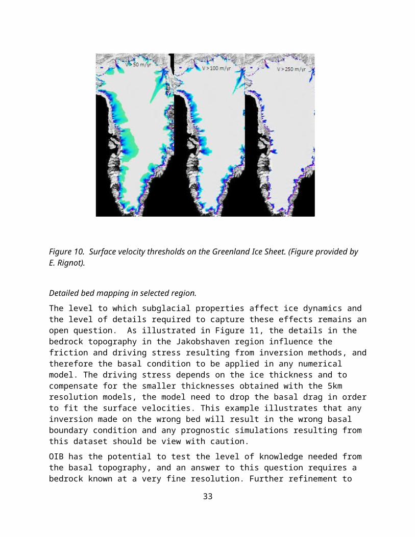
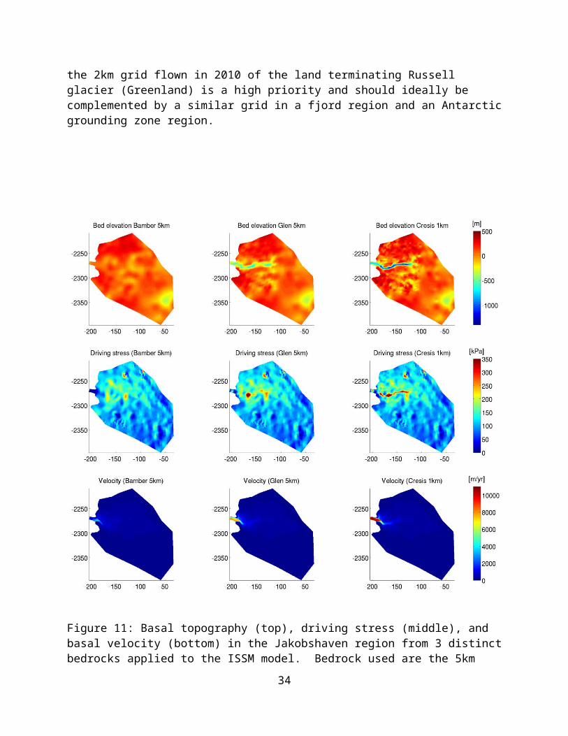
The level to which subglacial properties affect ice dynamics and the level of details required to capture these effects remains an open question. As illustrated in Figure 11, the details in the bedrock topography in the Jakobshaven region influence the friction and driving stress resulting from inversion methods, and therefore the basal condition to be applied in any numerical model. The driving stress depends on the ice thickness and to compensate for the smaller thicknesses obtained with the 5km resolution models, the model need to drop the basal drag in order to fit the surface velocities. This example illustrates that any inversion made on the wrong bed will result in the wrong basal boundary condition and any prognostic simulations resulting from this dataset should be view with caution.

OIB has the potential to test the level of knowledge needed from the basal topography, and an answer to this question requires a bedrock known at a very fine resolution. Further refinement to the 2km grid flown in 2010 of the land terminating Russell glacier (Greenland) is a high priority and should ideally be complemented by a similar grid in a fjord region and an Antarctic grounding zone region.

23

Figure 11: Basal topography (top), driving stress (middle), and basal velocity (bottom) in the Jakobshaven region from 3 distinct bedrocks applied to the ISSM model. Bedrock used are the 5km Bamber dataset (left), the 5km (middle) and the 1km (right) SeaRISE datasets that incorporates the fine scale Cresis data. Figure courtesy of Mathieu Morlinghem, Helene Seroussi, S. Nowicki, E. Larour.

Whole ice sheet and regional models.

To improve prognostic predictions of future sea-level contribution from the ice Greenland and Antarctic ice sheets obtained with whole ice sheet models, IOB is required to continue measurements that fill the gap in our current knowledge in bedrock elevations over coastal regions. OIB is required to make bedrock measurements on a 5km grid over areas of slow flow, and on a grid of the order of at least the ice thickness for regions of fast flows, or regions of complex stress regime (eg: grounding line or shear margins). Priority should be given to regions

24

where it is suspected that canyons might be present, or regions with bedrock below sea-level that could connect to the interior of the ice sheet (ie: high risk regions for ice loss).

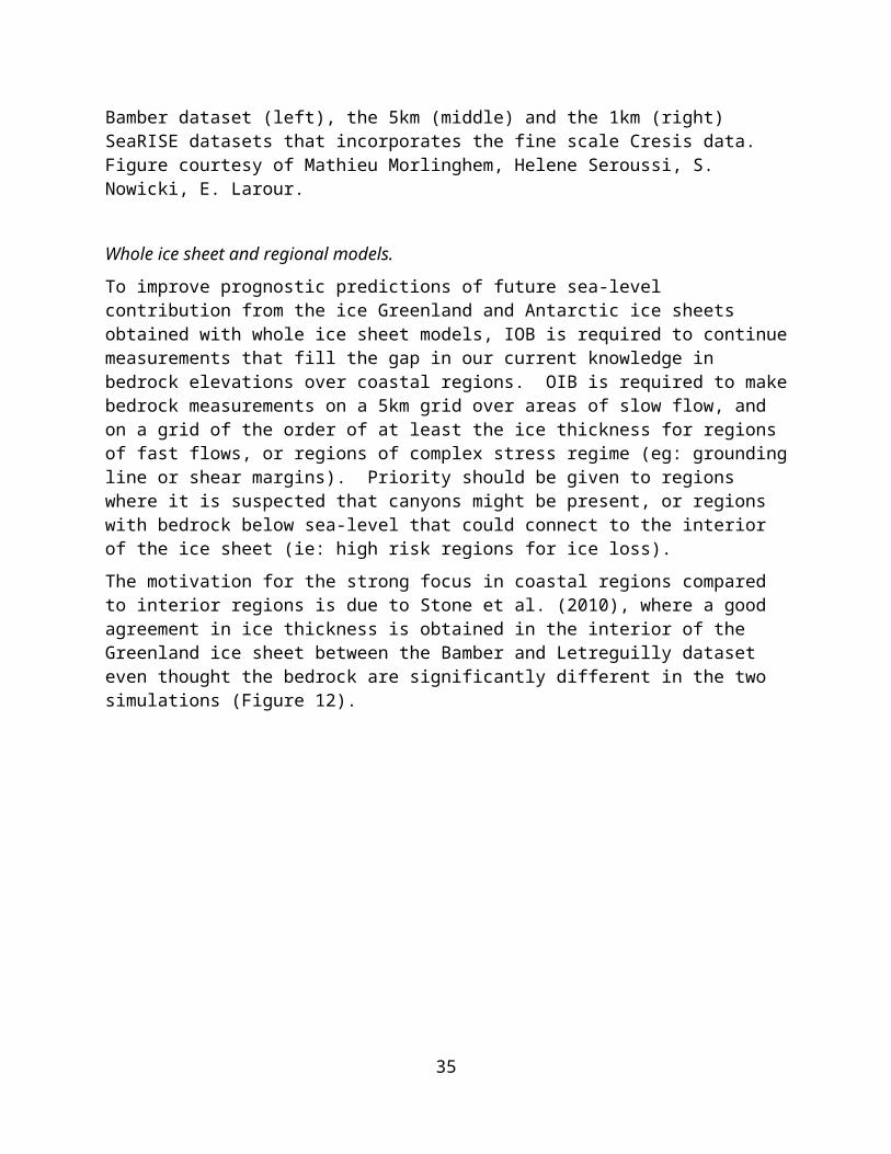
The motivation for the strong focus in coastal regions compared to interior regions is due to Stone et al. (2010), where a good agreement in ice thickness is obtained in the interior of the Greenland ice sheet between the Bamber and Letreguilly dataset even thought the bedrock are significantly different in the two simulations (Figure 12).

Figure 12: The ratio of the difference in ice thickness (a) and bedrock topography (b) between the Bamber and Letreguilly datasets expressed as a percentage (z_bamber – z_letreguilly/z_letreguilly). Figure adapted from Stone et al. (2010).

The motivation for more refined bedrock measurement in regions of fast or complex flow is based on experience with the SeaRISE simulations, where a 5km bedrock in the Jakoshaven region produced from the fine scale Cresis measurements (see Figure 11 “Glen 5km”) is necessary in order to reproduce a surface velocity similar to the observed velocity. These regions are also regions where the coarse resolution of whole ice sheet models often prevents them from reliable diagnostic or prognostic simulations, such that regional models have an important role.

Flow band models.

Continue the time series annually in a few selected regions with existing long term measurements (ex: Helheim Glacier or Jakobshavn Isbrea). These regions allow a study of the dynamics of glacier retreat and inversion of surface properties and elevation could provide insight on whether the basal condition are changing in time, or to test our current understanding of the underlying physics at play.

25

IS12) For Antarctica, important mass balance and dynamical changes are associated with processes occurring at the grounding line – the boundary where the inland ice sheet begins to float on the ocean - or ice sheet land terminus (ISMASS, 2003). (Figure 13). Therefore OIB shall make measurements of surface elevation, ice thickness and gravity along the grounding line and along a parallel track approximately 10 km upstream of the grounding line. The data will be crucial for ice flux measurements and to investigate dynamical processes at the grounding line. The two tracks are required partly because grounding likely occurs over a zone and partly to increase information available for ice dynamics models (e.g. surface and basal topography gradients). Success will constitute the first, complete circum-ice-sheet measurements of ice thickness and basal topography. Combined with surface velocity data acquired using spaceborne synthetic aperture radar data, the data will enable the most accurate estimate of the total volume flux of ice being discharged from the ice sheet in the vicinity of the ice margin or grounding line. Differencing the ice flux across our flight path with the integrated accumulation rate over the interior surface will provide an independent estimate of total ice sheet volume change.

Figure 13. Radarsat Antarctic Mapping Project (RAMP) coast line (green), ASAID grounding line (yellow courtesy of R. Bindschadler) overlain on RAMP coherence mosaic. The Riiser-Larsen Ice Shelf grounding line is distinguishable in the coherence data by the dark band separating the smooth ice shelf from the textured interior ice sheet. The ASAID grounding line and the coherence band generally agree to about 3 km in this area. Map provided by K. Jezek.

IS13) The vast majority of the largest Greenland glaciers terminate in the ocean and melt in contact with the ocean waters. Recent studies suggest that this melt process is orders of magnitude larger than at the surface and probably plays a central role in glacier stability, grounding line retreat and ice calving. A better understanding of these ice-ocean interactions and their impact on glacier is essential to interpret recent changes in glacier mass balance and in turn ice sheet mass balance, and also to improve our predictive capability of ice sheet evolution. Taken another way, we will not be able to predict glacier and ice sheet evolution at all until we

26

have made major progress in our understanding and characterization of these interactions.

To achieve this goal, it is critical to document the sea floor bathymetry in front of the glaciers as this determines the pathways for ocean heat to reach land ice. This includes the determination of the depth of the glacial fjords, the presence of sills from past grounding line positions, the presence of troughs generated by paleo ice streams, the exact depth of the fjords at the glacier front and how troughs and pathways are connected to the sea floor bathymetry on the surrounding continental ice shelf.

While data exist on the continental ice shelf, most glacial fjords in Greenland have never been surveyed (figure 14). Similarly, we have no sounding of the sea floor underneath floating ice shelves in the northern part of Greenland where ice-ocean interactions also play a fundamental role in glacier mass balance and evolution.

Therefore OIB shall collect measurements of the sea floor bathymetry in front of glaciers terminating in the ocean, in the glacial fjords extending to the mouth of the fjords where sills are usually present, and underneath floating ice shelves in the north. This will require at least a survey flight along the main axis of the fjords and a series of cross-fjord profiles as permitted by the local geography and time constraints on the mission. The goal is to determine the dominant geometric characteristics of these fjords to help better constrain ocean numerical models aiming at modeling ocean-fjord circulation and heat exchanges, with obvious implications for the modeling of ice-ocean interactions and glacier flow.

Figure 14. Bathymetry tracks used to do the best compilation todate of Arctic sea floor bathymetry, in particular around Greenland. See attached plot from IBCAO. Apart from southwest Greenland and fjords in east Greenland, the coastline is particularly devoid of data within 100-200 km of the coast (e.g. northwest Greenland, Kennedy channel in north Greenland,

27

northeast greenland, and the area between Kangerdlugssuaq and Helheim Glaciers). bathymetry tracks have been used to do the best compilation todate of Arctic sea floor bathymetry, in particular around Greenland. (Plot is from IBCAO and provided by E. Rignot).

IS14) Measurements of the distribution of suglacial water have been made since the 1970’s using ice sounding radar (Kapitsa and others, 1996) and also radar and laser altimeters. Essentially, ice sounding radar data collected over large subglacial lakes reveal smooth, highly reflective basal topography. Flow over subglacial lakes also results in characteristically smooth surface topography that is detectable with radar and laser altimetry. Radar interferometry and laser altimetry have also been used to measure changes in lake volume by detected elastic deflection of the ice sheet surface as subglacial lakes drain (Gray and others, 2005, Fricker and others, 2007) . For thinner water layers or for sparsely distributed water, reflectivity data from ice sounding radars have also been used to map water distributions but this analysis is complicated by the several parameters that contribute to the final radar intensity (basal roughness, temperature dependent absorption through the ice). Consequently radar tends to remain an uncertain proxy indication for basal water

IS15) Submeter, stereo mapping photography will contribute to better crosss track slope corrections of altimeter data in coastal regions of Greenland and Antarctica where slope-magnitudes are highest and where the surface is complicated by crevassing. While stereo mapping will qualitatively improve the IceBridge data set, the quantitative improvement is still unknown because of overall accuracy uncertainties and the amount of data that can be reasonably processed from what could be a very voluminous data set.

6.2. Ice Sheet Projected Requirements

(1) Accumulation rate estimates are essential to flux gate estimates of mass balance, but the extent to which these measurement can be applied and the need for additional in situ data is required are poorly characterized. Accumulation rates contribute to the uncertainty in flux gate, gravity, and altimetry measurements, making the ability measure them highly desirable. While the ability to determine such rates is currently experimental, the collection of the radar data by OIB will provide an extremely important data set for developing and validating the methods for accumulation retrieval.

Equation 1 under (IS1) illustrates that there are 7 distinct error terms contributing to the error in ice sheet thickening rate. Taking 15 cm/yr as the basin-averaged thickening rate accuracy, then each of the error terms on the right side of equation should be on the order of (15/(7)1/2) cm/yr of ice equivalent or about 6 cm/yr ice equivalent. This immediately gives an approximate bound on the required accuracy for the surface and basal mass balance (6 cm/yr ice equivalent). At sub-basin scales, the accuracy requirement is 4 cm/yr ice equivalent.

2) Subglacial water production and water migration are important controls on glacier flow. Techniques for measuring water distribution, distribution change and volume are successful for characterizing larger bodies of water (such as altimeter estimates of changing subglacial lake

28

volumes). However techniques to sample the distribution of thin water layers and to directly estimate water production are still immature (Oswald and Gogineni, 2008). Models can be used to try and infer water production rates. Basal hydrostatic pressure gradients can be used to estimate locations where water will pond. Additional research is needed to effectively use current and future models to guide development of robust direct measurement methods.

(3) Annual sampling is adequate but seasonal sampling would improve understanding of the stochastic processes that are superimposed the long term thickness change signal. Spatial and temporal sampling in the interior of Antarctica is more difficult because although accumulation and accumulation driven changes in density are less, dynamic thinning is also much less. Roughness is similar. A solution is to average over much larger areas than near the coast (100x100 km or more is the Cryosat estimate) and over longer periods of time than just one year (3 years or more).  Note that while thinning at a point in the interior is less than at a point on the coast, the area of the interior is huge so a little thinning can result in a big overall mass change.

4) Geothermal heat flux is critical, unmeasured parameter in the basal heat balance beneath glaciers (Fahnestock and others, 2001. Other parameters such as basal drag can be inferred from modeling but no similarly robust technique is available for heat flux estimates. Magnetics suffices in some instances as a proxy indicator of changing heat flux magnitudes, but accurate estimates of the flux magnitude are difficult to obtain with any existing method other than direct sampling at boreholes.

5) Subglacial lakes are distributed across much of Antarctica. Lake discharge is believed to be directly responsible for changes in glacier motion (for example recent speed ups of Byrd Glaciers). Ice sounding radars and laser altimeters have been successfully used to map lake locations and to measure lake volume changes with time. The primary challenge for further lake studies is to have detailed (km scale surveys) and repeat measurements (months) to study lake processes. These requirements pose difficult logistical challenges that may only b e addressable with UAV type platforms.

6) Enhanced free air gravity is required to better map sea floor bathymetry down stream of marine terminating glaciers. Current systems mounted on the NASA P-3 and DC-8 aircraft are limited to features with wavelengths on the order of 10 km. A challenge for the future it so develop approaches that reduce the measurable wavelengths to several km.

7) As mentioned above the primary challenge demonstrating the utility of stereo photography to IceBridge ice sheet science is developing processing schemes for reducing a voluminous photographic data set into digital elevation models with absolute elevation and slope accuracies sufficient to measurably improve cross track slope correction on altimeter data. A second challenge is demonstrating whether stereo photography can be used for glaciologically meaningful elevation change measurements.

6.3. Sea Ice Baseline Requirements Justification

SI 1. Make surface elevation measurements of the water, ice, or snow with a shot-to-shot independent error of less than 10 cm and correlated errors which contribute less than 1 cm to

29

the mean height error in either sea surface or sea ice elevation. The spot size should be 1 m or less and they should be spaced 3 m or less.

The primary purpose of the surface elevation measurements over sea ice is to obtain regional estimates of the sea ice thickness distribution. The thickness distribution is required, as opposed to a simple mean ice thickness, because of the nonlinear thermodynamic and dynamic processes important for the evolution of the ice pack. The community standard length scale for determining the thickness distribution, for example from submarines, is 50 km, as this length scale provides adequate opportunity to detect different ice types within a region and is small enough to resolve regional differences (Wadhams, 2002; Percival et al. 2008). The thickness distribution should be resolved to 10 cm bins in order to delineate level ice from ridged ice and in order to track changes in the mode of the distribution, since the mode often represents the thermodynamically dominated thickness. With 10 cm resolution, bins with as little as 5% of the area might have significant impact on the interpretation of the thermodynamic or dynamic properties of the ice pack. To adequately characterize these bins, the areal coverage for each bin should be resolved to less than 1%. Hence we end up with a basic requirement that the thickness distribution be determined with a resolution of 10 cm and an uncertainty of 1% or less for the fraction in each bin.

However there are many sources of error in determining the ice thickness from surface elevation measurements including the discrimination of leads, determining the presence of thin ice in leads, interpolating water levels to ice-covered regions, geoid levels, and snow depth (Kwok and Cuningham, 2008; Kurtz et al., 2009). Most of these sources of error are beyond the control of the measurement system, so here we only consider the errors that are due entirely to the measurement system. We determine the measurement requirement for optimal conditions…a canonical ice cover…and realize that in practice the ice thickness estimate errors may be larger due, for example, to wide spacing between leads, small isolated leads, or uncertainties in the snow depth.

The ice thickness hi is related to the freeboard hf of the ice as

hi=ρw hf

ρw−ρi

where ρw and ρi are the densities of water and ice. The ice thickness and uncertainties in the ice thickness are roughly 10 times those of the ice freeboard because the freeboard only represents about 1/10th of the ice thickness. The average freeboard for a set of laser shots over the ice is

h f=hi−hw

where hi and hw are the mean heights of the Ni ice shots (where N is the number of shots) and the nearby Nw open water shots. The errors associated with each of these mean heights arise from determining the mean from a finite number of observations, each of which has an independent and normally distributed error sh and an additional error due to the spatial correlation of the errors, ew and e i , such as might arise from a slowly varying error in the

30

knowledge of the reference system for the aircraft attitude or altitude. Based on data collected over ice sheets the shot-to-shot vertical precision of the ATM instrument is about sh = 10 cm (Krabill et al. 2002) which we take as the independent error. The error in the freeboard is then

For the thickness error to remain below 10 cm, sf must remain below 1 cm. The number density of shots for the ATM instrument when the aircraft is flying low over sea ice is approximately 30000/km. In the case of a 10-m lead across the width of the swath the number of water shots is Nw = 300. Assuming an adjacent ice class occupies 100 m of the swath, then Ni = 3000. This implies that the error in the freeboard due to the independent errors is just 0.03 cm. The uncorrelated errors add little to the mean freeboard error because of the potentially large number of observations for leads or ice classes. The smaller number of shots within very small leads will increase the freeboard errors from this source, and a sh value of 5 cm for the projected requirement will allow for the use of smaller leads. A 10-cm error, 1-m spot size, and 3-m spacing (similar to that of the ATM) are required to allow for adequate discrimination and use of small leads assuming lead identification can be corroborated with visual, or preferably also thermal, high resolution images with a pixel size of 50 cm or smaller.

If we assume the contribution of the independent errors is negligible and that ew and e i are equal and independent, both must be less than 0.71 cm to keep the error in the freeboard less than 1 cm. If they are correlated at very low frequencies or if the lead density is high so that the water level is determined from the average of several leads, the impact of the correlated errors will be smaller. In addition the elevation errors should ideally be independent of the reflectivity of the surface so that both leads and ice surfaces are equally well measured. Figure SI-1 shows a swath of ATM elevation data overlaying a visible image from the DMS camera.

Projected requirement SIP-1. Improve sea ice baseline requirement 1 to make surface elevation measurements with a shot-to-shot accuracy of 5 cm (versus 10 cm), assuming uncorrelated errors.This higher accuracy will allow for the use of smaller leads and a better definition of the sea surface elevation.

31

sf=√ sh2

Nw+

sh2

N i+ew

2 +e i2−2ew ei

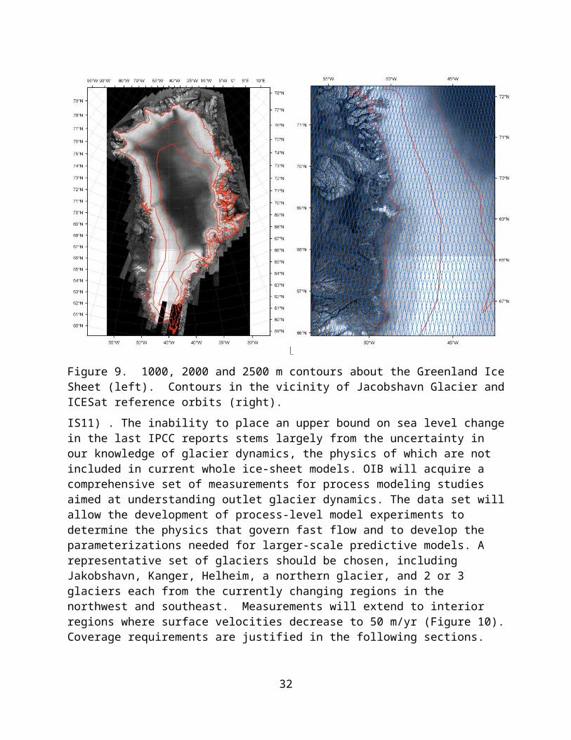
Figure SI-1. ATM elevation measurements superimposed on a DMS visible image showing the alignment with a large lead (figure by N. Kurtz). This figure also demonstrates the loss of ATM returns over open water leads, as well as a drop in measurement density over dark grey nilas.

SI 2. Make elevation measurements of both the air-snow and the snow-ice interfaces to an uncertainty of 3 cm, which enable the determination of snow depth to an uncertainty of 5 cm.

Determining accurate snow depth is important both for determining the ice thickness and for mapping the distribution of snow over sea ice with a spatial coverage never before obtained. Snow is an important element in determining the thermal conductivity of the ice, the surface albedo and the evolution of melt ponds. Given the roughly ten-fold increase in the error of the ice thickness from the error in the snow depth (Kwok and Cunningham, 2008), an error of less than 1 cm would be desirable, but it is not possible for a single radar return.

The snow depth (hs) is the difference in elevation between the air-snow (has) and snow-ice (hsi) interfaces:

hs = has – his

For the Ultra Wideband snow radar, the range resolution is ~5 cm (free space propagation) (Panzer et al., 2010). Assuming we can locate the snow-ice interface and the air-snow interface to ~3 cm (sas=ssi , half the range resolution) and we have an uncertainty of 0.1 g/cm3 in snow

32

density (this translates into ~10% uncertainty in the speed of light in snow), then the uncertainty in snow depth over N radar pulses,

ss=(1. 0+sc)√(sas2 +ssi

2 )/ N

This assumes a nominal snow density of 0.3 g/cm3. For σc = 0.1 (the fractional uncertainty in the

speed of light in snow) and a single return N=1, the expected uncertainty in snow depth is ~4.7 cm. However, if the air-snow interface were weakly scattering and more difficult to locate (sas is larger), then the per-pulse performance would degrade. Whether we can average over N pulses to produce a better estimate depends on the correlation length scale of the snow cover at the 10-20 m pulse-limited spot size of the snow radar.

For a given radar return, the most important parameters are the range precision and the range resolution. We wish to have the platform be stable at the 500 m length scale (to centimeters) to ensure that the motion compensation processing provides sufficient precision such that it would not introduce significant variability in the pulse-to-pulse averages. This can be relaxed if the radar platform is stable over a longer flight segment. Figure SI-2 shows an example of the snow radar returns with the surface elevation estimated from the ATM data. While the top of the snow surface is well represented, the ice surface is harder to distinguish at all locations.

For determining the snow depth for each freeboard estimate, further research is required to know how to assign the nadir snow depth measurements to the swath ATM measurements. This extrapolation will be the source of further error in the snow depth and ice thickness estimates.

Figure SI-2. Snow radar returns with the top snow surface profile derived from the ATM added as a black line (figure by R. Kwok).

SI 3. Provide annual acquisitions of sea ice surface elevation in the Arctic and Southern Oceans during the late winter in regions of the ice pack that are undergoing rapid change. Flight lines shall be designed to ensure measurements are acquired across a range of ice types including seasonal (first-year) and perennial (multiyear) sea ice to include, as a minimum:

33

Arctic

a) At least two transects to capture the thickness gradient across the perennial and seasonal ice covers between Greenland, the central Arctic, and the Alaskan Coast.

Some of the most rapid changes in Arctic pack ice are seen in the Beaufort Sea and in the thick ice in the central Arctic Ocean (Lindsay and Zhang, 2005). To the extent possible given the limited coverage of the OIB program it is important to provide continuous monitoring of these rapidly changing regions. Much of the Beaufort Sea is transitioning from perennial ice to seasonal ice so previous observations of the ice characteristics in this region may need to be revised. Two long transects across the central Arctic Basin connecting the northern coasts of Greenland and Alaska will sample the ice thickness gradient across both the first-year and multi-year ice packs such that a representation of ice types in the Beaufort Sea is obtained. These transects are designed to provide data that will contribute to an assessment of the condition of the Arctic ice pack (e.g. the thickness distribution and relative amounts of multiyear and seasonal ice) on a yearly basis.

b) The perennial sea ice pack from the coasts of Ellesmere Island and Greenland north to the pole and westward across the northern Beaufort Sea.

The thick multiyear ice in this region is experiencing the most rapid thinning in the Arctic Ocean [Maslanik et al., 2007; Comiso et al., 2008; Farrell et al., 2009] and it is critical to continue observations in this region to record potential on-going thinning. In addition, the ice draft in this region has traditionally been under sampled by submarine transects since it lies outside of the data release area and is rarely visited by ice breakers because of the consolidated thick ice. No moorings are deployed here. For this reason any additional OIB ice thickness observations in this region are a particularly important contribution to our understanding of the changes going on in the Arctic pack ice. Continued monitoring of the multiyear ice pack in this region is needed to track the loss of older ice and its replacement by younger second-year or first-year ice. Flight lines will be designed to survey an area that includes the ice pack directly north of Greenland and Ellesmere Island, west toward Queen Elizabeth and Banks Islands, and north towards the North Pole.

c) Sea ice across the Fram Strait and Nares Strait flux gates.

The Fram and Nares Straits are the two most important locations for ice export from the Arctic Ocean. In order to better constrain the rate of ice export, knowledge of the ice thickness across the Straits is required. While single transects cannot be used to determine the time-averaged flux, the thickness measurements can be used to asses the errors in model estimates of the ice thickness and, hence,the ice flux. An ongoing monitoring effort to measure ice flux will provide a budget for winter-time loss of sea ice volume from the Arctic Ocean to the North Atlantic Ocean.

d) The sea ice cover of the Eastern Arctic north of the Fram Strait.

34

This region is the location of the transpolar drift stream, the major conduit for ice exiting the Arctic Ocean via Fram Strait. Much of this ice originated on the Siberian shelves or in the Beaufort Gyre. Monitoring the thickness of this ice will help establish the rate of ice production far upstream.

Figure SI3 shows examples of the suggested flight tracks, in this case the actual flights flown in the spring of 2009 and 2010, along with an estimate of the mean ice thickness from the PIOMAS model (Polar Ice and Ocean Modeling and Assimilation System, Zhang and Rothrock, 2003). The flights sample the thick multiyear ice near the Greenland and Canadian coasts and the thinner ice in the Beaufort Sea.

Figure SI3. Flight tracks from 2009 and 2010 along with estimates of the mean ice thickness from the PIOMAS model for the month of March.

Antarctic

a) The sea ice of the Weddell Sea between the tip of the Antarctic Peninsula and Cape Norvegia.

IceBridge measurements over sea ice will extend the record of observations begun by ICESat such that continued monitoring of a key transect across the Weddell Sea will be conducted on a yearly basis. Ice export from the Weddell Sea is typically computed along a “flux-gate” which spans the Weddell Sea from the northeastern tip of the Antarctic Peninsula to Cape Norvegia. An IceBridge transect between these two points will provide gradients in ice thickness along the flux-gate. The total volume of sea ice exported into the Antarctic Circumpolar Current is a combination of sea ice growth within the Weddell Sea, the inflow of sea ice from the eastern Weddell, and the ice produced in polynyas located in the southern Weddell.

b) The mixed ice cover in the western Weddell Sea between the tip of Antarctic Peninsula and Ronne Ice Shelf.

A transect across the mixed ice cover in the western Weddell Sea between the northern tip of the Antarctic Peninsula and the Ronne Ice Shelf will provide an optimal sampling of ice types in the Weddell Sea including first year ice in the northern Weddell, and multiyear ice in the southern Weddell. This transect will allow us to constrain the overall thickness distribution of the Weddell Sea ice pack and monitor any change in the state of the multiyear ice pack.

35

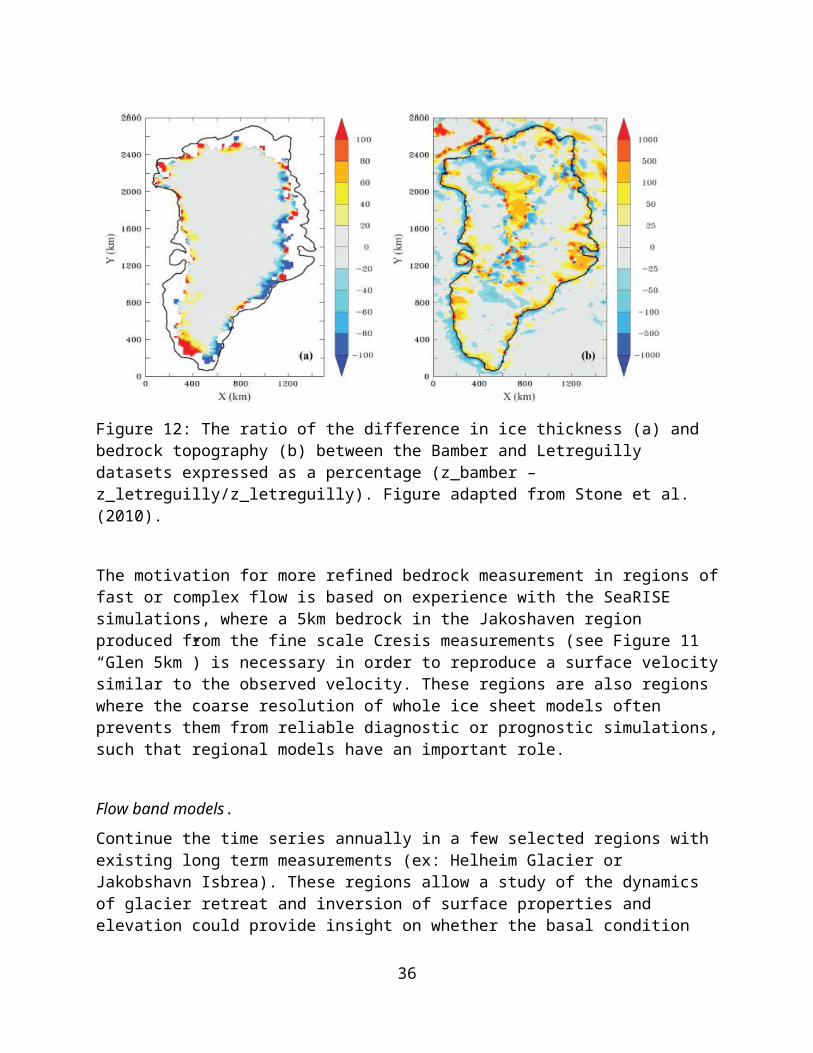
c) The ice pack of the Bellingshausen and Amundsen Seas.

The aim is to provide a constraint on the thickness distribution of the ice pack buttressing the West Antarctic Ice Sheet (WAIS). This region exhibits high variability in sea ice extent, and potentially thickness, where such variability is linked to the modes of the Southern Oscillation. The flight line shall be repeated on a yearly basis to establish a multi-year record of sea ice thickness in this region.

Projected requirement SIP 2. Extend sea ice baseline requirement 3 to other regions of the Arctic and Southern Oceans:

Arctic (to better constrain estimates of sea ice volume change) North Pole region Southern Beaufort Sea, west of Banks Island Sea ice along the east coast of Greenland Southern Chukchi Sea north of Bering Strait Davis Strait Lancaster Sound and other parts of the Canadian Archipelago

Antarctic (to better understand the process of sea ice formation and snow accumulation) Ross Sea Surveys of areas of polynya formation, over and downwind of the polynya Surveys of areas where katabatic winds may deposit abundant snow.

SI 4. Include flight lines for sampling the ground tracks of satellite lidars (ICESat-1 and ICESat-2) and radars (CryoSat-2 and Envisat) and, in the case of CryoSat-2, both IceBridge and CryoSat-2 ground tracks should be temporally and spatially coincident whenever possible. At least one ground track of each satellite should be sampled per campaign.

The lapse in basin-scale monitoring of Arctic and Southern Ocean sea ice as a result of the delay between the end of the ICESat mission in late 2009 and the launch of ICESat-2 planned for 2016 will result in a gap in the long-term laser altimetry record over sea ice. CryoSat- 2, launched in early 2010, will help bridge this data gap to some extent, although the SAR/Interferometric Radar Altimeter (SIRAL) onboard will result in surface elevation measurements that are inherently different to those of the ICESat laser system (GLAS). IceBridge should include flight tracks that are spatially and temporally coincident with CryoSat-2 so as to improve our understanding of the differences between the laser (ICESat/ICESat-2) and radar (CryoSat-2) altimetric signals over sea ice. Further, it will allow placement of IceBridge data in the wider context of the CryoSat-2 dataset.

As a lower priority, a portion of IceBridge flights shall be designed to refly ground tracks of Envisat radar altimetry data and historical ICESat laser altimetry. This data is helpful in providing a continuation of the long-term sea ice altimetry record in regions where the ice thickness distribution has already been established over a 5-6 year time-period. This will also allow for better interpretation of changes in the sea surface elevations related to changes in

36

circulation and fresh water content and to increase our confidence that the changes are not associated with the unmodeled geoid variability.

SI 5. Conduct sea ice flights as early as possible in the flight sequence of each campaign, preferably prior to melt onset.

Sea ice flights will be conducted at sea ice maximum extent (March – early April in the Northern Hemisphere; late September – early October in the Southern Hemisphere) to obtain winter-time data that is consistent with the limited operation periods of the ICESat laser campaigns (typically late February-March, and October-mid November). Furthermore, the likelihood of data acquired by the two IceBridge airborne radars, Ku-band and snow, being predominantly from the snow-ice interface [Beavan et al. 1995] is increased and thickness estimation improved if sea ice flights occur when snow cover is cold and dry, i.e. before the onset of the melt season.   The dielectric properties of snow can be controlled by its liquid water content at temperatures above –5 °C [Willatt et al., 2010].  In order to mitigate the impact of a large variability in snow grain size on radar altimetry measurements over sea ice, we recommend that measurements are made before the onset of spring melt over both Arctic and Southern Ocean ice packs; air surface temperatures typically increase around late April in the Arctic and mid-October over Southern Ocean sea ice.The likelihood of getting the bulk of the radar returns from snow-ice interface within Antarctic sea ice is reduced relative to the Arctic due to flooding events in the Antarctic. Therefore our timing requirements are relaxed somewhat for Antarctic, i.e., we are resigned to higher liquid water content.

SI 6. Collect coincident natural color visible imagery of sea ice conditions at a spatial resolution of at least 10 cm per pixel to enable direct interpretation of the altimetric data.

Establishing the height of the open ocean surface is essential for determining the freeboard and hence the ice thickness (see S1 justification). The open water level is found from leads within the ice pack and these can be unambiguously determined from visible imagery. The leads in visible imagery appear dark compared to the ice and are easily identified. Visible images are a minimum requirement and high resolution (1-m) thermal images are a desirable projected requirement (see SIP 3).

Projected requirement SIP 3. Collect thermal images for a swath that, as a minimum, covers the LVIS data swath with a resolution of 0.5 m or better, and are calibrated to brightness temperature with an accuracy of 0.1K.

There can be a skim of thin newly frozen ice within the leads that is sometimes not apparent in the visible imagery. However, this ice can be identified in infrared images when the temperature of the lead is below the freezing point of sea water. The temperature of the thin ice, when compared to that of the thick ice, can be used to estimate the thickness of the lead ice. Since we cannot estimate the thickness of the thin lead ice identified in visible images, thermal images would help to establish this. Visible images are a minimum requirement and high resolution (1-m) thermal images are a highly desirable projected requirement in this regard.

37

Projected requirement SIP 4. Improve sea ice baseline requirement 6 to collect coincident digital stereo imagery of sea ice conditions at a spatial resolution of at least 10 cm (versus 20 cm) per pixel, at a vertical resolution of 20 cm.

Stereo imagery will enable direct interpretation of the altimetric data and provide a complimentary surface elevation product.

SI 7. Conduct sea ice flights primarily in cloud-free conditions. Data shall be retained under all atmospheric conditions with a flag included to indicate degradation or loss of data due to clouds.

Ideally IceBridge sea ice flights will be conducted under cloud-free conditions to obtain accurate visible imagery of the surface and to limit the effects of forward scattering on laser altimetric measurements. However, data should be retained under all atmospheric conditions and a flag should be included to indicate degradation or loss of data due to clouds. This will enable investigators to understand the impact of cloudy returns on elevation accuracy from laser altimetric data, whereby atmospheric optical depth can be directly related to surface elevation accuracy. This will support data simulations in preparation for the ICESat-2 mission.

SI 8. Make precise full gravity vector measurements on all low-elevation (< 1000 m) flights over sea ice to enable the determination of short-wavelength geoid fluctuations (in a waveband of order 10 to 200 km) along the flight track to a allow the calculation of the geoid to a precision of 2 cm.

An accurate, detailed knowledge of the marine geoid is critical for confident separation and isolation of the sea surface and sea ice topography signals in the IceBridge altimeter observations. Short-wavelength errors in our current knowledge of the marine geoid exceed 25 cm in a waveband of order 10 to 200 km over many areas of the Arctic Ocean. However IceBridge’s full-vector gravimetric (AirGRAV) observations can be used to isolate and reduce these geoid errors along flight tracks and to improve models of the Arctic marine geoid.

SI 9. Actively seek out and coordinate with field campaigns that are consistent with IceBridge project objectives.

Ground truth data from field campaigns will help to determine uncertainties in the OIB estimates of the snow depth and ice thickness (see S1 and S2 justifications). Ground truth data is the only way to obtain independent verification of the measurements obtained from the airborne instruments. In addition, aircraft survey data provided by OIB enables field data to be placed in a wider context. Such activities will substantially augment OIB outreach efforts and supports international collaboration. In all cases data sharing agreements must be in place.

SI 10. Make available to the community instrument data on sea ice surface elevation and snow depth within 3 months of acquisition and derived products within 6 months of data acquisition.

The utility of the OIB data for assessing and understanding the rapid changes we are seeing in the sea ice of the Arctic will be greatly enhanced if the data are made available to the science community as soon as possible after acquisition. Estimates of the ice thickness can be compared

38

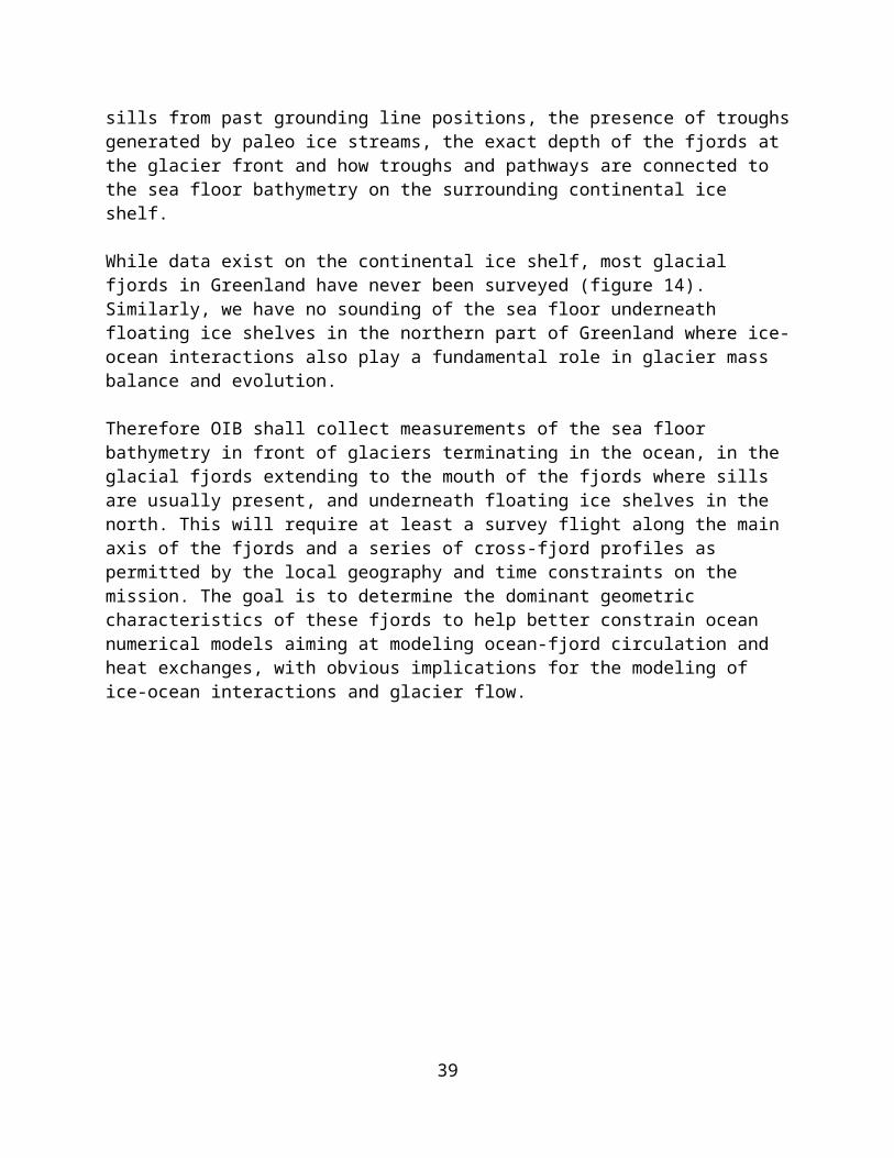
to recent retrospective model estimates to ascertain if the models are in error and to determine if model projections might be biased. In addition, any information that can help document or explain current ice conditions will contribute to OIB outreach efforts.

Projected requirement SIP 5. IceBridge shall support the validation of operational sea ice analysis and forecast products by providing estimates of sea ice freeboard within 1 week of data acquisition and estimates of sea ice thickness within 2 weeks of data acquisition.

An accelerated release of sea ice thickness products in near real time will allow for their operational use by the National Ice Center and other entities that analyze and predict ice extent and thickness.

6.4. References

S. Anandakrishnan, D. D. Blankenship, R. B. Alley & P. L. Stoffa, 1998. Influence of subglacial geology on the position of a West Antarctic ice stream from seismic observations Nature 394, 62-65 (2 July 1998) | doi:10.1038/27889; Received 5 March 1997; Accepted 10 March 1998.

R.E. Bell, D.D. Blankenship, C.A. Finn, D. Morse, T. Scambos, J.M. Brozena, and S.M. Hodge, 1998. Influence of Subglacial Geology on the Onset of a West Antarctic Ice Stream from Aerogeophysical Observations, Nature, 394,  p. 58-62.

A.E. Block and R.E. Bell, 2011. Geophysical Evidence for Sof Bed Sliding at Jacobshaven Isbrae, Greenland, In review Cryosphere.

Brook, M., B. Brock, and M. Kirkbride, 2003. Glacial Outlet Valley Size – Ice Drainage Area Relationships: Some Considerations. Earth Surface Processes and Landforms, 28, 645-653.

Comiso, J. C., C. L. Parkinson, R. Gersten, and L. Stock (2008), Accelerated decline in the Arctic sea ice cover, Geophys. Res. Lett., 35, L01703, doi:10.1029/2007GL031972.

Fahnestock, M., Waleed Abdalati, Ian Joughin, John Brozena, and Prasad Gogineni (14 December 2001) High Geothermal Heat Flow, Basal Melt, and the Origin of Rapid Ice Flow in Central Greenland, Science 294 (5550), 2338. [DOI: 10.1126/science.1065370]

Farrell, S. L., S. W. Laxon, D. C. McAdoo, D. Yi, and H. J. Zwally (2009), Five years of Arctic sea ice freeboard measurements from ICESat, J. Geophys. Res., vol. 114, C004008, doi:10.1029/2008JC005074.

Fricker, H. A., Scambos, T., Bindschadler, R. & Padman, L. (2007), An active subglacial water system in West Antarctica mapped from space. Science 315, 1544-1548.

Giles, K. A., S. W. Laxon, D. J. Wingham, D. Wallis, W. B. Krabill, C. J. Leuschen, D. McAdoo, S. S. Manizade, R. K. Raney (2007), Combined airborne laser and radar altimeter

39

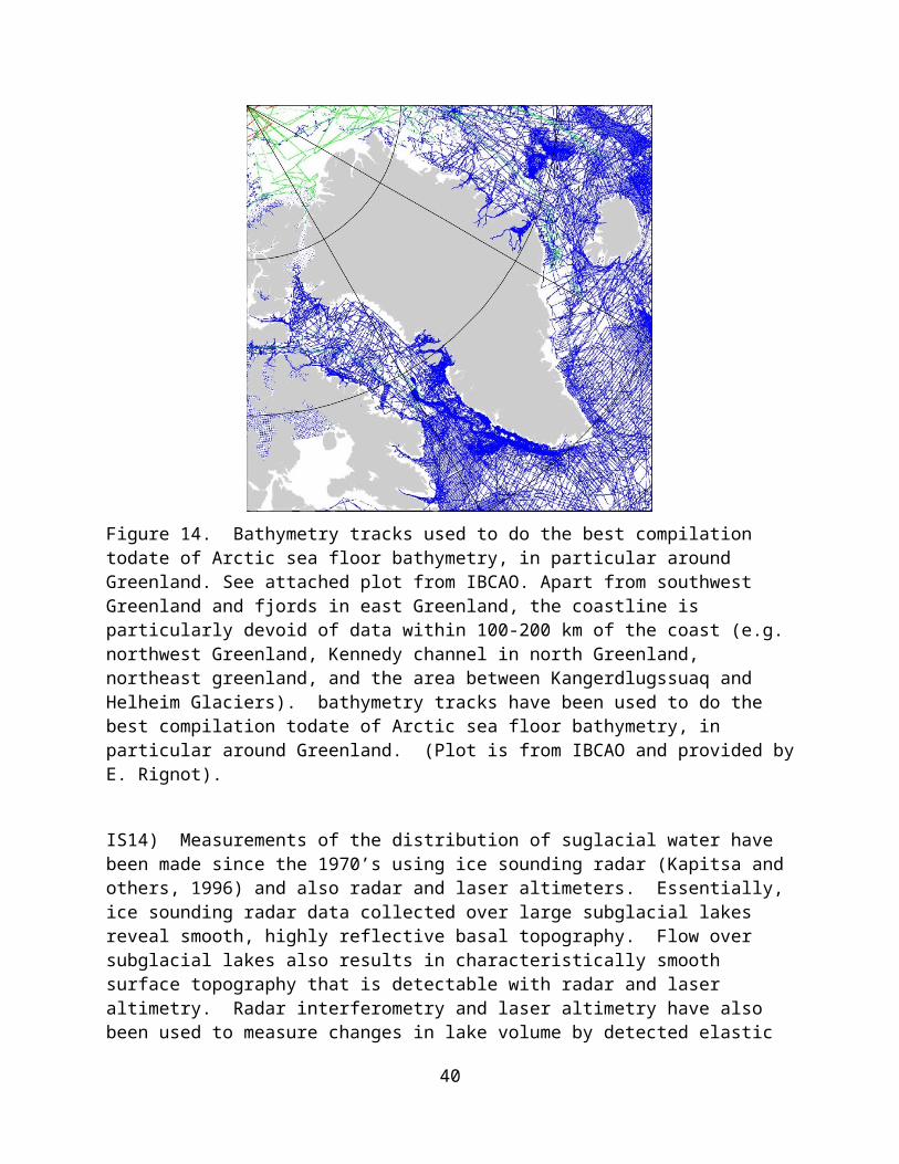
measurements over the Fram Strait in May 2002, Remote Sensing of the Environment, 111, 182–194.

Gray, L., I. Joughin, S. Tulaczyk, V.B. Spikes, R. Bindschadler, and K. Jezek, 2005: Evidence for subglacial water transport in the West Antarctic Ice Sheet though three-dimensional satellite radar interferometry. Geophys. Res. Lett., 32,L03501, doi:10.1029/2004GL021387.

IGOS, 2007. Integrated Global Observing Strategy Cryosphere Theme Report - For the Monitoring of our Environment from Space and from Earth. Geneva: World Meteorological Organization. WMO/TD-No. 1405. 100 pp.

ISMASS Committee, 2004: Recommendations for the collection and synthesis of Antarctic Ice Sheet mass balance data. Glob. Planet. Change, 42, 1-15.

Kapitsa, A.P., J. Ridley, G de Q Robin, M. Siegert, and I. Zotikov, 1996. A large freshwater lake beneath the ice of central East Antarctica. Nature, 381, 684-686

Krabill, W. B., W. Abdalati, E. B. Frederick, S. S. Manizade, C. F. Martin, J. G. Sonntag, R. N. Swift, R. H. Thomas, and J. G. Yungel (2002), Aircraft laser altimetry measurement of elevation changes of the Greenland ice sheet: technique and accuracy assessment, J. Geodynamics, 34, 357-376.

Kwok, R., G. F. Cunningham, M. Wensnahan, I. Rigor, H. J. Zwally, and D. Yi (2009), Thinning and volume loss of Arctic sea ice: 2003-2008, J. Geophys. Res., doi:10.1029/2009JC005312.

Kurtz, N. T., T. Markus, D. J. Cavalieri, L. C. Sparling, W. B. Krabill, A. J. Gasiewski, and J. G. Sonntag (2009), Estimation of sea ice thickness distributions through the combination of snow depth and satellite laser altimetry data, J. Geophys. Res., 114, C10007, doi:10.1029/2009JC005292

Kwok, R., and G. F. Cunningham (2008), ICESat over Arctic sea ice: Estimation of snow depth and ice thickness, J. Geophys. Res., 113, C08010, doi:10.1029/2008JC004753.

Lindsay, R. W. and J. Zhang, 2005: The dramatic thinning of arctic sea ice, 1988-2003: have we passed a tipping point?. J. Climate, 18, 4879-4894.

Maslanik, J. A., C. Fowler, J. Stroeve, S. Drobot, H. J. Zwally, D. Yi, and W. J. Emery (2007), A younger, thinner Arctic ice cover: Increased potential for rapid, extensive sea ice loss, Geophys. Res. Lett., 34, L24501, doi:10.1029/2007GL032043.

Neal CS; “The dynamics of the Ross Ice Shelf revealed by radio echo sounding,” Journal of Glaciology, 24(90), 295-307, 1979.

NRC Committee on Earth Science and Applications from Space, 2007. Earth Science and Applications from Space: National Imperatives for the Next Decade and Beyond. National Research Council, ISBN 0-309-66714-3, 456 p.

40

Oswald, G., P. Gogineni, 2008, Recovery of subglacial water extent from Greenland radar survey data. J. Glac, vol 54, no 184, p. 94-106

Percival, D. B., D. A. Rothrock, A. S. Thorndike, and T. Gneiting (2008), The variance of mean sea-ice thickness: Effect of long-range dependence, J. Geophys. Res., 113, C01004, doi:10.1029/2007JC004391.

Panzer, B., C. Leuschen, A. Patel, T. Markus, and P. Gogineni (2010), Ultra-wideband radar measurements of snow thickness over sea ice, Proc. 2010 IEEE International Geoscience and Remote Sensing Symposium (IGARSS), Honolulu, HI, 25 - 30 July 2010, 3130 – 3133, doi: 10.1109/IGARSS.2010.5654342.

Skolnik, M.I., 1962. Introduction to Radar Systems. McGraw-Hill Book Co.

Van der Veen and ISMASS, 2010. Ice sheet mass balance and sea level rise: A science Plan. SCAR Report 38, ISSN 1755-9030, 37 p.

Wadhams, P. (1997), Ice thickness in the Arctic Ocean: The statistical reliability of experimental data, J. Geophys. Res., 102(C13), 27,951–27,959.

Zhang, J., and D.A. Rothrock: Modeling global sea ice with a thickness and enthalpy distribution model in generalized curvilinear coordinates, Mon. Wea. Rev., 131(5),  681–697, 2003.

41