Embed Size (px)
Citation preview
International Council for the Exploration of the Sea
Conseil International pour l’Exploration de la Mer
H. C. Andersens Boulevard 44–46 · DK-1553 Copenhagen V · Denmark
Telephone + 45 33 38 67 00 · Telefax +45 33 93 42 15 www.ices.dk · [email protected]
ICES Cooperative Research Report
Rapport des Recherches Collectives
No. 268
August 2004
The DEPM Estimation of Spawning-Stock Biomass for Sardine and Anchovy
Compiled and Edited by
Yorgos Stratoudakis Miguel Bernal IPIMAR
Avenida de Brasilia P-1449-006 Lisbon
Portugal
Instituto Espapañol de Oceanografia
Centro Oceanográfico de Malaga
Apdo 285 Puerto Pesquero s/n 29640 Fuengirola
Spain
Andrés Uriarte AZTI
Herrera kaia, Portualde z/g 20110 Pasaia (Gipuzkoa)
Spain


Recommended format for purposes of citation: ICES. 2004. The DEPM Estimation of Spawning-Stock Biomass for Sardine and Anchovy. ICES Cooperative Research Report, No. 268. 91 pp. For permission to reproduce material from this publication, please apply to the General Secretary.
ISBN 87–7482–018–4 ISSN 1017–6195

Contents
1 Introduction ................................................................................................................................................................ 5 1.1 Background..................................................................................................................................................... 5 1.2 Contributions .................................................................................................................................................. 5 1.3 Report structure............................................................................................................................................... 5
2 DEPM surveys for sardine and anchovy .................................................................................................................... 5 2.1 Introduction..................................................................................................................................................... 5 2.2 DEPM surveys for sardine (Sardina pilchardus) ............................................................................................ 6
2.2.1 Atlantic waters (Iberian Peninsula)................................................................................................... 6 2.2.2 Mediterranean waters........................................................................................................................ 6
2.3 DEPM surveys for anchovy (Engraulis encrasicolus)................................................................................... 6 2.3.1 Atlantic Waters (Bay of Biscay) ....................................................................................................... 6 2.3.2 Mediterranean waters........................................................................................................................ 7
2.4 The 2002 Atlanto-Iberian sardine survey........................................................................................................ 7 2.4.1 Survey details.................................................................................................................................... 7 2.4.2 Egg production estimation ................................................................................................................ 8 2.4.3 Adult parameter and spawning biomass estimation.......................................................................... 8 2.4.4 Spatial structure in recent sardine DEPM surveys and comparison with acoustics .......................... 9
2.5 The 2002 Biscay anchovy survey ................................................................................................................. 11 2.5.1 Survey details.................................................................................................................................. 11 2.5.2 Egg production estimation .............................................................................................................. 11 2.5.3 Adult parameters and spawning biomass estimation ...................................................................... 12 2.5.4 Comparison with previous estimates and general considerations ................................................... 13
3 GAMS in DEPM estimation..................................................................................................................................... 31 3.1 Introduction................................................................................................................................................... 31 3.2 Methodology................................................................................................................................................. 31
3.2.1 Egg ageing ...................................................................................................................................... 31 3.2.2 Sea area and survey limits estimation ............................................................................................. 33 3.2.3 Model fitting and selection ............................................................................................................. 33 3.2.4 Model prediction and variance estimation ...................................................................................... 34 3.2.5 Software.......................................................................................................................................... 34
3.3 Application to sardine and anchovy DEPM surveys..................................................................................... 35 3.3.1 Sardine ............................................................................................................................................ 35 3.3.2 Anchovy.......................................................................................................................................... 37
3.4 GAMS in adult parameter and biomass estimation: a first example ............................................................. 39 3.4.1 Sardine ............................................................................................................................................ 39 3.4.2 Anchovy.......................................................................................................................................... 39
3.5 Discussions and recommendations ............................................................................................................... 40 4 Other advances in DEPM methodology ................................................................................................................. 54
4.1 The Continuous Underway Fish Egg Sampler (CUFES).............................................................................. 54 4.1.1 Introduction..................................................................................................................................... 54 4.1.2 Summary of results from PELASSES............................................................................................. 55
4.1.2.1 CUFES and CalVET/PAIROVET experi-mental sampling........................................... 55 4.1.2.2 CUFES as a quantitative sampler of egg abundance in the water column ..................... 56
4.1.3 The use of CUFES in the 2002 sardine DEPM survey ................................................................... 56 4.1.4 Using CUFES to test DEPM assumptions ...................................................................................... 57 4.1.5 Recommended use of CUFES in future DEPM surveys................................................................. 57
4.2 Egg staging and ageing ................................................................................................................................. 57 4.2.1 Staging workshop ........................................................................................................................... 57 4.2.2 Analysis of new and published egg incubation data for sardine and anchovy ................................ 58
4.2.2.1 Anchovy......................................................................................................................... 58 4.2.2.2 Sardine ........................................................................................................................... 59
4.2.3 Factors other than temperature affecting egg development ............................................................ 59 4.2.4 Assumptions on daily spawning ..................................................................................................... 60
4.3 Sardine reproduction off Iberia ..................................................................................................................... 61 4.3.1 Maturity .......................................................................................................................................... 61
4.3.1.1 Clarification of definitions ............................................................................................. 61 4.3.1.2 Comparison of macroscopic and microscopic maturity stages ...................................... 62 4.3.1.3 Maturity stages to be included in the estimation of spawning biomass ......................... 62
ICES Cooperative Research Report, No. 268 3

4.3.2 Spawning season and dynamics...................................................................................................... 62 4.3.2.1 Spawning activity........................................................................................................... 62 4.3.2.2 Spawning dynamics off Portugal ................................................................................... 63
4.4 POF dating and spawning fraction estimation .............................................................................................. 64 4.4.1 Sampling bias.................................................................................................................................. 64 4.4.2 POF staging and ageing .................................................................................................................. 65
5 References ................................................................................................................................................................ 84 6 Annexes.................................................................................................................................................................... 88
Annex I: Reference collection of sardine (Sardina pilchardus) egg stages. Staging based on Ahlstrom (1943). .... 88Annex II: Reference collection of anchovy (Engraulis encrasicolus) egg stages. Staging based on Moser, and
Ahlstrom (1985)....................................................................................................................................... 89 Annex III: Reference collection of sardine (Sardina pilchardus) POF daily cohorts. ............................................. 90 Annex IV: Reference collection of anchovy (Engraulis encrasicolus) POF daily cohorts. ..................................... 91
ICES Cooperative Research Report, No. 268 4
1 Introduction
1.1 Background Lasker (1985) provides the first and most thorough re-port on the use of the Daily Egg Production Method (DEPM) for the estimation of the spawning biomass of small pelagic fish stocks. An update to this report is pro-vided by Anonymous (1997), a compilation of research papers resulting from an EU concerted action on DEPM techniques. The present Cooperative Research Report is intended to complement to the above publications, re-viewing the use of the method for sardine and anchovy in European waters and describing very recent develop-ments in specific areas of DEPM sampling and estima-tion. Its contents are predominantly drawn from the most recent report of the ICES Study Group on the Estimation of Sardine and Anchovy Spawning Biomass (SGSBSA) that met in Malaga (Spain) during the summer of 2003 (ICES, 2003b). In addition, it includes sections from the first SGSBSA report that resulted from a meeting in Lis-bon (Portugal) during the autumn of 2001 (ICES, 2002).
1.2 Contributions The SGSBSA reports were based on valuable contribu-tions from several national and international research projects, as well as the personal experience of the 24 sci-entists that participated in the two group meetings. Statis-tical methodology for the most appropriate use of egg in-cubation data in stage/age models, the ageing of staged eggs and the modelling of daily egg production and mor-tality through GAMs were developed as part of an EU project on GAMs (Study 99/080, http://www.ruwpa.st-and.ac.uk/depm/index.html) that was concluded within 2003. Additional research in the use of CUFES in ich-thyoplankton surveys and a workshop for the calibration of sardine and anchovy egg staging were performed within the EU project PELASSES (EU Study 99/010). Most surveys presented in this report took place with the financial support of the EU. A sardine incubation ex-periment was performed by IEO (Spain) as part of na-tional research activities, while most of the recent activi-ties in Portugal (IPIMAR) were performed as part of the research project PELAGICOS (http://ipimar-iniap.ipimar.pt/pelagicos). Miguel Bernal (Spain), Emilia Cunha (Portugal), Leire Ibaibarriaga (Spain), Concha Franco (Spain), Paz Jimenez (Spain), Ana Lago de Lan-zós (Spain), José Ramon Pérez (Spain), Luis Quintanilla (Spain), Maria Santos (Spain), Alexandra Silva (Portu-gal), Yorgos Stratoudakis (Portugal) and Andres Uriarte (Spain) contributed to the preparation of both SGSBSA reports, while Pablo Carrera (Spain), Kostas Ganias (Greece), Alberto García (Spain), Daniel Gaughan (Aus-tralia), John Hunter (USA), Mike Lonergan (UK), Placida Lopes (Portugal), Immaculada Martin (Spain), Cristina Nunes (Portugal), Eduardo Soares (Portugal), Yolanda Vila (Spain), and Juan Zwolinski (Portugal) contributed in one of the two reports. Finally, most of the methodological developments presented in Section 3 re-sulted from the valuable contribution of Simon Wood,
David Borchers, Mike Lonergan and Camila Dixon (all from the University of St Andrews, Scotland).
1.3 Report structure Section 2 summarizes existing information on DEPM applications for sardine and anchovy in European waters. Sampling and estimation is described in more detail for the most recent surveys (2002) performed in Atlantic wa-ters for sardine and anchovy and already reported to the SGSBSA. Section 3 is dedicated to the application of GAMs in DEPM estimation, summarizing and extending the findings of the EU project on GAMs that most Study Group members participated in. The underlying theory is briefly reported and the method is illustrated through worked examples, based on the sardine and anchovy sur-veys presented in the previous section. Section 4 con-siders advances in other methodological aspects of DEPM estimation. The first part of this section is dedi-cated to issues related to egg production sampling and estimation (use of CUFES, staging and ageing, etc.), while the second part is dedicated to adult parameters, with emphasis on sardine. Section 5 provides a compre-hensive (but not exhaustive) reference list, while An-nexes 1–4 provide illustrations from reference collec-tions of egg and post-ovulatory follicle (POF) stages for sardine and anchovy.
2 DEPM surveys for sardine and anchovy
2.1 Introduction The first part of the Section (Sections 2.2–2.3) summa-rizes the DEPM surveys that have been performed for sardine and anchovy in European waters. Emphasis is given to applications in Atlantic waters (where DEPM estimates are used routinely in stock assessment), but a brief description of known applications in the Mediterra-nean are also provided. The second part of the chapter (Sections 2.4 and 2.5) describes the most recent surveys in Atlantic waters (2002) in more detail, in order to demonstrate the survey and estimation methodology applied. Estimates are based on the traditional methods (Lasker, 1985; Hunter and Lo, 1997), which continues to provide the standard estimates of spawning-stock biomass for the purposes of stock assessment. However, results for 2002 should be compared to those obtained by the application of GAMs (Sections 3.3 and 3.4 for sardine and anchovy respectively), although GAM estimates of adult parameters and SSB are necessarily provisional (given that they were applied for the first time during the course of the most recent SGSBSA meeting). In the case of sardine, estimates based on mean survey values are compared to post-stratified and GAM-based estimates to clarify whether inappropriate sampling design under spatial structure in abundance and adult parameters can lead to biased biomass estimates (Stratoudakis and Fryer, 2000; ICES, 2002). In the case of anchovy, the presence of sufficient spatial structure to justify post-stratification for 2002 is explored and the results are compared with the long series of DEPM
ICES Cooperative Research Report, No. 268 5
long series of DEPM estimates and the acoustic results for 2002.
2.2 DEPM surveys for sardine (Sardina pilchardus)
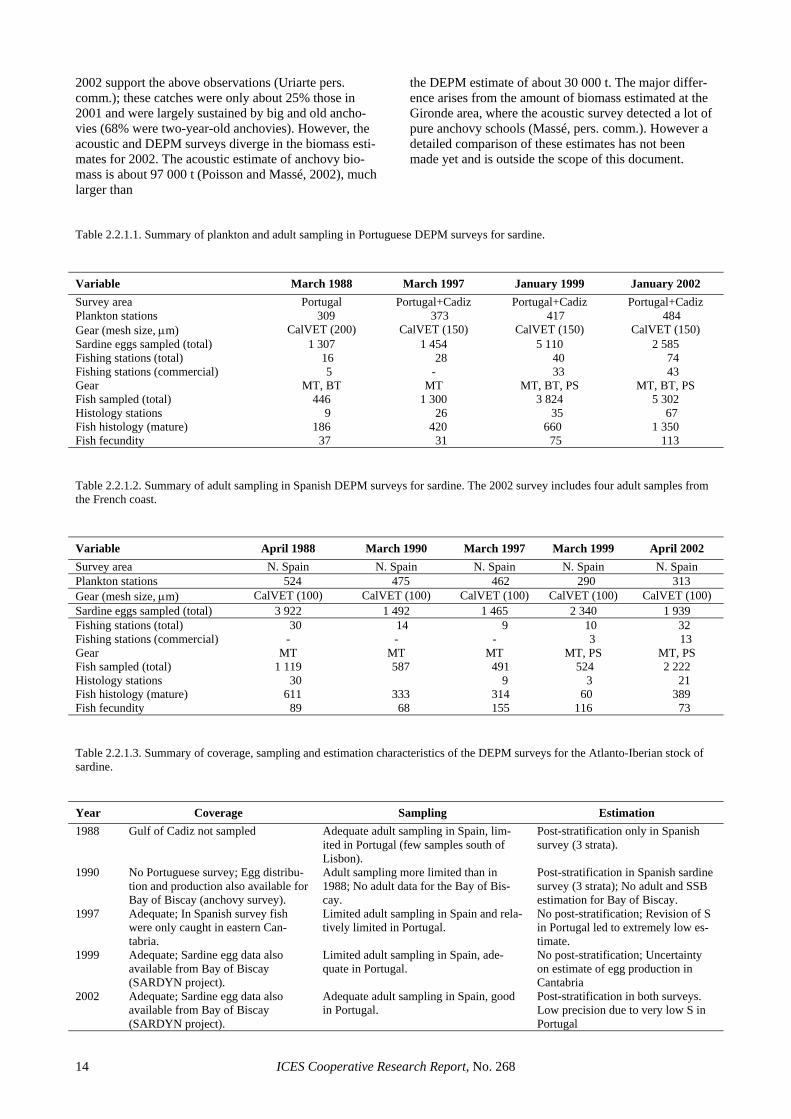
2.2.1 Atlantic waters (Iberian Peninsula) The method was first used to estimate the spawning bio-mass of the Atlanto-Iberian sardine stock in 1988 (Cunha et al., 1992; García et al., 1992) and then repeated in 1990, 1997, 1999 and 2002, based on coordinated sur-veys by Portugal and Spain (García et al., 1991; García et al., 1993; Cunha et al., 1997; Lago de Lanzós et al., 1998; Stratoudakis et al., 2000; Bernal et al., 2000; ICES, 2000; ICES 2002; ICES 2003b). Up to 1999 the surveys were based on informal contacts between IPIMAR (Portugal) and IEO (Spain). Since 2000 surveys are planned and executed under the auspices of ICES on a triennial basis (the next survey is planned for 2005 with financial support from the EU). Tables 2.2.1.1 and 2.2.1.2 provide sampling details for the sardine DEPM surveys performed until now by Portugal and Spain re-spectively, while Table 2.2.1.3 summarizes the coverage, sampling and estimation characteristics of each survey. The latter table demonstrates that the entire distribution area of the Atlanto-Iberian stock of sardine has only been sampled since 1997 (in 1988 the Gulf of Cadiz was not sampled and in 1990 there was no survey in Portugal). Further, the only survey where sampling intensity was good throughout the stock area, both for eggs (see Figure 2.4.1.1 for distribution of plankton samples) and adults (see Figures 2.2.1.1 and 2.2.1.2 for spatial distribution of adult samples in all Portuguese and Spanish DEPM sur-veys respectively) was the most recent one (2002). Ta-bles 2.2.1.4–2.2.1.9 provide the estimates of egg produc-tion, mean female weight, batch fecundity, sex ratio, spawning fraction and spawning biomass respectively for all surveys (details on sampling and estimation in ICES 2000; ICES, 2002; ICES, 2003b and Section 2.4 of this report).
2.2.2 Mediterranean waters The DEPM was recently applied to estimate the spawn-ing biomass of sardine in the central Aegean and Ionian Seas (Somarakis et al., 2001; Ganias, 2003). This was the first reported application of the DEPM to Mediterra-nean sardine, and presented particular interest and diffi-culties due to the peculiar topography of the survey area (many small-sized semi-enclosed gulfs), the biological heterogeneity and the small size of the sardine popula-tions. Table 2.2.2.1 shows the spawning biomass and DEPM parameter estimates. Since the stocks of sardine in the central Aegean and Ionian Seas exhibited different spawning peaks, the survey area was geographically stratified.
Daily egg production was estimated using both eggs and yolk-sac larvae in order to improve the precision of the estimate. Batch fecundity was measured in hydrated, tertiary-yolk globule and migratory nucleus females be-cause in Mediterranean sardine there exists a well-defined hiatus between the advanced batch and the stock
of smaller oocytes in the tertiary yolk-globule stage (Ganias et al., 2004). The histological examination and comparative analysis of sardine follicles revealed three classes of POFs: day-0 (0–9.5 hrs), day-1 (24–33.5 hrs) and day-2 (48–57.5 hrs). Despite differences in season and temperature regimes, batch fecundity and spawning fraction estimates from the Aegean and Ionian Sea were similar. Compared to existing values for the Atlanto-Iberian sardine stock, the estimates of spawning fraction and relative fecundity were slightly lower in the Mediter-ranean, despite considerable differences in the mean fe-male weight between Mediterranean and Atlantic popu-lations.
2.3 DEPM surveys for anchovy (Engraulis encrasicolus)
2.3.1 Atlantic Waters (Bay of Biscay) The DEPM has been regularly applied to the Bay of Bis-cay anchovy to estimate its biomass and population numbers at age (Motos et al., 1991; Motos and Uriarte 1991; Motos 1994; Motos and Uriarte 1994; Motos 1996; Uriarte 2001). The series of DEPM estimates spans the period 1987–2003 (with a single gap in 1993) and is routinely used by ICES for the assessment of the Bay of Biscay anchovy stock (e.g. ICES 2003a). These surveys have been undertaken by AZTI in cooperation with the Spanish (IEO) and French (IFREMER) insti-tutes of marine research (Uriarte et al., 1998; Uriarte et al., 1999a; Uriarte et al., 1999b).
In order to obtain estimates of daily egg production and specific fecundity, two surveys (an egg and an adult cruise) have usually been carried out at peak spawning time (May/June) over the expected spawning area of the Bay of Biscay anchovy population. This area extends over the Southeast area of the Bay of Biscay, with limits at 5ºW in the Iberian Coast and at 47ºN in the French Coast (e.g. Figure 2.5.1.1). Adult sampling during the survey (e.g. Figure 2.5.1.2) is usually complemented with samples taken opportunistically on board the Span-ish and French commercial fishing fleets of purse seiners and pelagic trawlers (Uriarte et al., 1996). In 1987, 1988, 1996, 1999 and 2000 no adult surveys took place and in those cases the opportunistic sampling obtained through the commercial fleet was the only source for adult infor-mation: in the first two years, commercial samples were used to derive the daily fecundity estimates of the popu-lation, whereas in the latter three years those samples were not used at all and a regression method assuming constant daily fecundity were used instead. The total set of DEPM estimates is presented in Tables 2.3.1.1 and 2.3.1.2.
Egg sampling is based on the CalVET net (Smith et al., 1985) and follows a systematic central sampling scheme. Eggs from both CalVET samplers are used in the analysis (Uriarte and Motos, 1998), often giving rise to the term PAIROVET to distinguish from applications where only one CalVET sampler is used. From the whole set of adult samples gathered during the adult survey, a subset is chosen for final processing with the criterion of the capture date being within ±5 days of the egg sam-
ICES Cooperative Research Report, No. 268 6
pling in the same area. The opportunistic adult samples from the fleet permit to expand the area of sampling coverage. In general, a broad spatial structure is evident in the adult population, with smaller fish tending to be closer to the shore. This leads generally to post-stratification of the DEPM estimation procedure (for P0 and adult parameters), with two or three spatial strata be-ing defined according to depth. Adult parameters are unweighted averages of the strata. An extensive review and description of DEPM adult parameter estimation is provided in Uriarte et al. (1999a). Finally, the DEPM formulation has been extended to provide spawning-stock population at age (SSPa) estimates with variances inferred from the delta method (Uriarte, 2001). Sen-sitivity analyses on the influence of the stratification and weighting factors are routinely performed. Regression methods for the estimation of SSB in the absence of adult sampling have been applied since 1996 (Uriarte et al., 1999a, b) based on the relationships between spawn-ing area, daily egg production per unit surface and the biomass obtained in years where complete DEPM is ap-plied.
2.3.2 Mediterranean waters The DEPM has been used to evaluate the anchovy spawning biomass of the Catalan Sea in 1990 (Palomera and Pertierra, 1993), Catalan Sea-Gulf of Lions in 1993 and 1994 (García and Palomera, 1996; Olivar et al., 2001), Ligurian-North Tyrrhenian seas in 1993 (García and Palomera, 1996), Aegean sea in 1993 (Tsimenides et al., 1995) and 1999 (Somarakis et al., 2002), Ionian Sea in 1999 (Somarakis et al., 2002), south-western Adriatic sea in 1994 (Casavola, 1998), and Sicilian Channel in 1998, 1999 (Quintanilla and García, 2001) and 2000 (Quintanilla, pers. comm.).
Spawning biomass and DEPM parameters estimates in the Mediterranean show high variability both within (inter-seasonal and inter-annual variations) and between regions (Table 2.3.2.1). Different methodologies can par-tially explain these variations. In the Aegean Sea, where exceptionally high egg production estimates were found in 1993, oblique Bongo tows were used instead of the vertical CalVET tows and the spawning area was not en-tirely covered. Also, different temperatures were used to assign ages to eggs in different regions (sub-surface tem-perature in the Aegean Sea, mean temperature of the first 10 m or 20 m in the Sicilian Channel and Catalan Sea re-spectively). Sampling with purse seiners instead of pe-lagic trawls, and commercial instead of research vessels in the Aegean and Catalan Seas, could restrict the sam-pling to commercial fishing grounds and explain some adult parameter differences. The use of the methodology of Laroche and Richardson (1980) instead of the hy-drated oocyte method (Hunter et al., 1985) may explain the high relative fecundity in the Catalan Sea. Differ-ences in spawning fraction estimation method could also explain some inter-regional differences in this parameter.
Overall, the parameters with the highest variance are the daily egg production (P) and the spawning fraction (S), while the large variation in egg mortality rates should also be noted. The temperature range during the peak spawning period may vary from 16° to 25°C in
some Mediterranean areas. Egg development duration and post-ovulatory follicle degeneration can present great differences within this temperature range, thus af-fecting these parameter estimates.
2.4 The 2002 Atlanto-Iberian sardine survey
2.4.1 Survey details The most recent DEPM survey for Atlanto-Iberian sar-dine took place in 2002, covering the entire distribution area of the Atlanto-Iberian stock. The region from the Gulf of Cadiz to the northern Portugal/Spain border (Minho River) was surveyed by IPIMAR, while IEO sampled the north and north-western Iberian Peninsula and the Bay of Biscay (up to 45°N). The Portuguese sur-vey (7 January – 8 February 2002) was carried out on-board RV “Noruega”, while the Spanish survey (18 March – 6 April 2003) was conducted onboard RV “Cornide de Saavedra” for the plankton component and RV “Thalassa” for the adult component.
Both national surveys consisted of ichthyoplankton sampling on fixed (CalVET) and underway (CUFES) stations (Figure 2.4.1.1). The CalVET hauls were per-formed using a net with 150 µm mesh size, operating vertically from 150 m (Portugal) or 100 m (Spain) to the surface. In shallower areas, the net was towed from 5 m above the bottom to the surface. CUFES samples were used to delimit sardine spawning grounds and to modify adaptively the intensity of CalVET sampling. In the Por-tuguese survey, sampling depths and towing efficiency of the hauls were controlled with a sensor (Minilog) fit-ted on the net line; while sampled volume was calculated from towing length and stray angle (see ICES, 2002). Sea surface (3 m depth) temperature, salinity and fluo-rescence were determined using sensors located at the entrance of the CUFES concentrator, while broad indica-tions about the thermal structure of the water column were obtained by a Minilog sensor coupled to the CalVET net. In the Spanish survey, General Oceanics Flowmeters were used to record the towing length and estimate the sampled water volume (assuming a filtration efficiency of 100%), while a Minilog was used to record maximum sampling depth. A continuous record of tem-perature and salinity was obtained from a thermo-salinometer coupled to CUFES, while CTD profiles were obtained in each CalVET station.
Sardine eggs were identified and counted on board immediately after collection. All samples were fixed in 4% buffered formaldehyde solution for subsequent veri-fication of egg counts and staging in the laboratory. The decision on the distance between CalVET stations was based on presence or absence of sardine eggs on the pre-vious CalVET and/or CUFES stations. In total, 769 CalVET (473 in Portugal and 296 in Spain) and 1185 CUFES (546 in Portugal and 639 in Spain) samples were obtained during the surveys. Daily egg production was determined using data from the CalVET performed along transects spaced 8 nm apart. Within the same transect the distance between stations was 3 nm for CUFES sampling and varied between 3 and 6 nm for CalVET hauls. In the Spanish survey (that used for the first time CUFES on-
ICES Cooperative Research Report, No. 268 7
board RV “Cornide de Saavedra”) a calibration exercise was carried out in French waters (see Section 4.1.3) to test the performance of CUFES as a quantitative sampler. Finally, sardine egg incubation experiments were at-tempted in both surveys, but with poor results. In the Portuguese survey the eggs did not develop (showing morphological characteristics of unfertilized eggs), while in the Spanish experiment eggs only developed up to stage VI. In both cases mature sperm seemed to be a lim-iting factor, with few ripe males and small quantities of sperm being collected in hauls with large number of hy-drated females.
Adult fish samples (Figure 2.4.1.2) were obtained by demersal and pelagic trawls (research vessels) and purse seining (commercial vessels). Overall, 32 samples were obtained in the Spanish survey (4 in the French coast) and 74 in the Portuguese (roughly proportional to re-gional sardine abundance), providing the most compre-hensive adult DEPM sampling of the series. Most sam-ples were obtained in the inner shelf, with a mean fishing depth of 45 m. Random samples of 80 and 100 fish were aimed in the Spanish and Portuguese survey respectively (although most commercial samples off Portugal only contained 50 fish). For fish collected onboard the re-search vessels, biological sampling was immediately per-formed and gonads of macroscopically identified mature females were preserved in individual jars with formalde-hyde solution for further processing in the laboratory. Fish collected onboard commercial Portuguese vessels were immediately preserved and on land the abdomen was lightly slit to allow better fixation of the gonad. In the latter case, biological sampling was performed on preserved fish and conversion factors were applied to transform preserved to fresh weight. For the estimation of batch fecundity, extra hydrated females were collected in several hauls performed by the research vessels. Pre-served female gonads were treated histologically for the estimation of spawning fraction (Pérez et al., 1992a; Quintanilla and Pérez, 2000a) and the elimination of go-nads with POFs from the estimation of batch fecundity. Batch fecundity was estimated using the gravimetric method (MacGregor, 1957) by counting the hydrated oo-cytes (Hunter et al., 1985; Pérez et al., 1992b; Quintanilla and Pérez, 2000b; Zwolinski et al., 2001).
2.4.2 Egg production estimation Egg production estimates from the 2002 sardine surveys have already been reported (see Table 2.2.1.4 and ICES, 2003a). These estimates were used to obtain spawning biomass estimates for the Spanish and Portuguese sur-veys and to compare with GAM-based production esti-mates (see Section 3.3.1). However, to explore the im-pact of spatial structure in the 2002 survey, post-stratified estimates of egg production were obtained in the course of the last SGSBSA meeting (ICES, 2003b). These results are reported in Section 2.4.4.
2.4.3 Adult parameter and spawning biomass esti-mation
Sardine adult DEPM parameters and spawning biomass are separately estimated for the Portuguese and Spanish
survey of 2002, without considering their spatial struc-ture (i.e., without post-stratification), in line with the es-timates that have been provided so far for the 1997 and 1999 surveys (however, see Section 2.4.4). All estimates refer to mature fish (i.e., maturity stage II and above, ac-cording to the rationale described in Section 4.3.1.4), in-cluding those inactive. Estimation for the Spanish survey excludes the 4 adult samples that were collected in the French coast (outside the stock area).
Mean weight (W): In the Spanish survey, female weight was estimated from gonad-free weight using the linear model W = – 1.304+1.094 W* (R2 = 0.98). The model was fitted using data from 520 non-hydrated fe-males collected during the 2002 survey. Mean female weight in the Spanish survey was 75.0 gr (CV = 5%), using data from 28 hauls. The 2002 estimate is higher and considerably more precise than the 1999 one (66.0 gr, CV = 41%), when data from only 6 hauls were used. In the Portuguese survey, mean female weight was esti-mated from the observed female weight of non-hydrated fish (for rationale see ICES, 2003b). Mean female weight in the Portuguese survey was 44.3 gr (CV = 5%), using data from 70 hauls. The 2002 estimate is very similar to the 1999 one (44.4 gr, CV = 5%, n = 40). The lack of improvement in the precision of the 2002 estimate (de-spite the duplication of sampling effort) is largely due to the presence of very large fish in a single commercial haul off central Portugal. Removing this haul from the estimation leads to a slightly lower estimate of mean weight (42.9 gr) and increases its precision (CV = 3.7%, n=69). However, this haul was maintained in the final es-timation, since there was nothing apparently erroneous with this outlier.
Batch fecundity (F): In total, 113 hydrated females without post-ovulatory follicles (POFs) were available for batch fecundity estimation in Portugal and 73 in Spain. In Spain, estimation followed the standard weighted linear regression model (batch fecundity as a function of gonad-free weight (W*), weighted by the in-verse of W*) and the following relationship was ob-tained: Spanish 2002 survey: F = -3255 + 436.25 W* (R2 = 63%) The standard error was 713 for the intercept and 38.9 for the slope. The intercept estimate was non-significant (t =-1.113, p> 0.05). If the relationship is forced through the origin, the slope (which then provides an estimate of relative fecundity) is 394.2 with a standard error of 9.4. Following the above model, mean batch fecundity for the 2002 Spanish survey was estimated to be 26089 (CV = 6%).
In Portugal, 2 linear (with and without weighing) and two generalised linear models (with a Gamma or a nega-tive binomial error distribution and an identity link) were considered (Table 2.4.3.1). The model parameters and the resulting mean estimates of batch fecundity were very similar in all cases (the largest discrepancy in mean batch fecundity was <0.5% among the four models con-sidered). However, the two GLMs led to higher propor-tions of explained variation, had smaller standard errors associated to the parameter estimates and provided con-siderably improved residual inspection plots (Figures
ICES Cooperative Research Report, No. 268 8
2.4.3.1 and 2.4.3.2). For estimation purposes, the GLM with a Gamma distribution and an identity link was cho-sen, given that a model with the same parameterisation has also been successfully used to describe mackerel fe-cundity (Darby, pers. comm.): Portuguese 2002 survey: F = -4286.2 + 464.3 W* (R2 = 81%). Following the above model, mean batch fecundity for the 2002 Portuguese survey was estimated to be 14 255 (CV = 6%). Figure 2.4.3.3 shows the relationship between female weight and batch fecundity in the 2002 survey in comparison to all previous sardine DEPM surveys. It clearly shows that relative fecundity in 2002 was signifi-cantly lower than in previous years, and relative fecun-dity was the lowest ever reported off Portugal. For the Portuguese 2002 survey, this agrees with other indicators (see Section 4.3.2.2) to suggest that the survey took place during uncharacteristic conditions for sardine spawning. However, relative fecundity was also low in the March 2002 Spanish survey, probably indicating bioenergetic limitations in sardine reproduction during that year.
Spawning fraction (S): Spawning fraction was esti-mated using the composite sample of day 1 and day 2 POFs. In total, 352 ovaries from 19 hauls were used in the Spanish survey and 1350 ovaries from 67 hauls in the Portuguese survey. The estimated spawning fraction for the Spanish survey was 0.127 (CV = 21%) and for the Portuguese survey 0.030 (CV = 21%). In both cases, these are the lowest spawning fractions ever reported. In the Portuguese case, this is probably the lowest S esti-mate that has ever been reported for a sardine species during peak spawning. A consequence of this very low estimate is that the precision of the Portuguese estimate remains low, despite the effective duplication of the number of histologically examined ovaries. It should be noted that if S in 2002 had remained at the levels ob-served in 1999 (around 0.10), the increased level of adult sampling would have reduced the CV of this parameter estimate to around 10–12% (Picquelle, 1985).
Sex ratio (R): Sex ratio was estimated as the weight ratio of females in the mature population. Given that male gonads were only classified macroscopically, sex ratio was estimated based on individuals that were macroscopically identified in a maturity stage larger than I (i.e., traditional definition of mature fish for DEPM purposes). In total, 2222 mature fish were used for the estimation of sex ratio in the Spanish survey and 4481 in the Portuguese survey. The estimated sex ratio for the Spanish survey was 0.542 (CV= 9%) and for the Portu-guese survey 0.611 (CV = 3%). These estimates are very similar to those obtained in 1999, but in both surveys the 2002 estimates are more precise due to the larger number of independent samples.
Spawning-stock Biomass (SSB): Table 2.4.3.2 sum-marizes the DEPM parameter estimates for the Portu-guese and Spanish 2002 surveys respectively and calcu-lates the resulting estimate of spawning biomass. Over-all, the 2002 DEPM survey for the Atlanto-Iberian stock leads to an SSB estimate of 382.3 Ktonnes, with a CV of 37%. Despite the lowest ever egg production in sardine DEPM surveys, the 2002 estimate of SSB is the highest of the existing estimates, due to the particularly low daily
fecundity observed in that year. Also, despite the con-siderable intensification of sampling in both national sur-veys, the precision of the biomass estimate remains rela-tively low (for assessment purposes), mainly due to the low precision in the egg production and spawning fraction estimates.
The low precision in the egg production estimates seems to be partly inherent to the use of the traditional estimator. Section 3.3.1 shows that considerable im-provements in the precision of this parameter can be achieved through the use of GAMs, where CVs in the order of 20% or below are achieved without evidence of bias. This was also the case for 2002, where the GAM-based estimate reduced the CV of the Iberian egg pro-duction estimate to 16%. The precision in the spawning fraction estimate of the Spanish survey was close to that anticipated (Picquelle, 1985) for the observed level of sampling effort and spawning activity (S = 0.13, n = 19). However, the extremely low estimate of spawning frac-tion in the Portuguese survey was something that could have not been anticipated during the planning of the sur-vey, given that estimates below 6% had never been re-ported for sardine in peak spawning. The large sampling effort in the 2002 Portuguese survey and the wealth of auxiliary information collected along it, leave little doubt that the very low spawning fraction in 2002 resulted from unfavourable conditions to sardine spawning. De-spite the low levels of precision, the large sampling ef-fort in 2002 precludes the presence of sampling artefacts, suggesting that large inter-annual variations in spawning activity is an inherent feature of the Atlanto-Iberian stock of sardine. Further, the information collected in that sur-vey can contribute to improve the understanding on sar-dine spawning dynamics. For example, Figure 2.4.3.4 (left) shows that spawning activity during the Portuguese 2002 survey was very patchy, mainly concentrated in small areas of high phytoplankton densities (data ob-tained from CUFES), while Figure 2.4.3.4 (right) sug-gests that the smooth relation between chlorophyll fluo-rescence and observed spawning fraction (GAM with bi-nomial error distribution) is significant.
2.4.4 Spatial structure in recent sardine DEPM surveys and comparison with acoustics
Traditional estimation of spawning biomass in the DEPM is entirely based on the selected survey design, using design-based estimators. Judgement sampling has been recommended as a way of achieving sampling pro-portional to local fish densities and reliable estimation of spawning biomass when there are spatial differences in abundance and in the DEPM adult parameters. DEPM surveys for adult sardine parameters have been consid-ered to follow the principles of judgment sampling, using acoustic density as an indicator of local fish densities (Cunha et al., 1992; García et al., 1991; García et al., 1992; Cunha et al., 1997). However, the exact procedure for allocating sampling effort according to the acoustic signal has never been described, and in most surveys the regional allocation of sampling effort does not reflect the estimates of regional abundance obtained from the DEPM (Spain) or from acoustic surveys (Portugal). In 1999, the Portuguese DEPM survey further deviated
ICES Cooperative Research Report, No. 268 9
from the principles of judgement sampling since, to in-crease sampling effort, additional samples were collected opportunistically from commercial vessels fishing near the research vessel.
In addition, a major assumption in DEPM estimation is that all parameters are constant over the range and du-ration of the survey. When this assumption is violated, Piquelle and Stauffer (1985) recommend post-stratification, where a series of strata is determined a posteriori and an estimation is performed independently for each stratum. Post-stratification has been used in the Spanish DEPM surveys of 1988 and 1990 (García et al., 1992; García et al., 1991), where considerable differ-ences in mean weight and spawning fraction were ob-served between Galician and Eastern Cantabria. In 1999 post-stratification was not considered in the Spanish DEPM surveys due to the small number of fishing sta-tions available per region. On the other hand, post-stratification has never been used in the Portuguese DEPM surveys. In 1988 and 1997 there was insufficient information to stratify (in 1988 there were only three fishing stations south of Lisbon). In 1999, post-stratification was not used for comparability with the previous two surveys (ICES, 2000).
Under an adequate survey design (i.e., sampling ef-fort proportional to local abundance), post-stratification should only lead to more precise estimates. Stratoudakis and Fryer (2000) demonstrated the impact of inadequate survey design and post-stratification on the DEPM esti-mation of sardine spawning biomass off Portugal in 1999. Post-stratifying the Portuguese 1999 DEPM survey into two strata (western and southern) increased the SSB estimate by nearly 50%. The origin of this large differ-ence was explored in a simulation exercise. A series of populations consisting of two strata were constructed, in which fish abundance and mean spawning fraction in each stratum were allowed to vary widely, and where egg production, sex ratio and batch fecundity were as-sumed known without error. Each population was sam-pled using simple random sampling and various forms of stratified random sampling (allocation proportional to survey area, to fish abundance, and optimal allocation). Ignoring spatial structure in spawning fraction led to very biased and imprecise estimates of fish abundance. In the population scenario that most closely resembled the 1999 Portuguese DEPM survey, the bias was –25%, suggesting that unstratified estimation underestimates the true SSB. Stratified random sampling with allocation proportional and optimal allocation outperformed alloca-tion proportional to area and were robust to moderate levels of misallocation.
To evaluate the impact of sampling effort allocation and spatial structure in the 2002 survey, estimation was repeated using post-stratification (Figure 2.4.4.1). Post-stratification in Portugal considered the two strata used by Stratoudakis and Fryer (2000), where the survey was divided into a western and a southern stratum. Post-stratification in Spain used the three strata previously considered by García et al. (1991 and 1992). Non-linear weighted least squares (nls library in R, weights to ac-count for the uneven spacing of samples) were used to obtain post-stratified estimates of egg production for the Portuguese 2002 survey. It should be noted that this es-
timator is not the one proposed by the Study Group (GLM estimator), but was maintained to obtain compa-rable results and concentrate on the impact of spatial structure in daily fecundity. Post-stratified estimates of egg production in the Spanish survey were obtained us-ing the recommended estimator (GLM with negative bi-nomial error distribution, an offset accounting for the ef-fective area of the sampler and weights to account for the uneven spacing of samples). To test the significance of post-stratification linear and generalized liner models (GLMs) were used for the 4 adult parameters, with stra-tum being the explanatory variable (2 and 3 level factor for the Portuguese and Spanish survey respectively). A linear model was used for female mean weight and batch fecundity, where observations were weighed by the number of mature females in each sample. A GLM with a binomial error distribution was used for spawning frac-tion and sex ratio, where the binomial denominator was the number of histologically examined females and the number of mature fish in the sample respectively.
Table 2.4.4.1 shows the post-stratified estimates of egg density, mortality and production for the Spanish and Portuguese 2002 surveys. Results are not provided for Galicia, since very few stations with eggs were observed, not permitting the fitting of a GLM. Also, the unstratified Spanish estimate is slightly higher than that reported in ICES (2003), due to modifications in the estimation of positive area and the use of stations rather than transects in estimation. Post-stratification led to an overall esti-mate of egg production 8% higher than under no stratifi-cation (6% higher in Portugal and 13% higher in Spain), but the two estimates are not significantly different. Ta-ble 2.4.4.2 shows the significance of the stratum effect in the models fitted to each adult parameter from the Portu-guese and Spanish 2002 surveys. In the Portuguese sur-vey, there is a significant spatial effect in mean female weight, which is also reflected in batch fecundity. In the Spanish survey, female weight and batch fecundity do not differ significantly among strata, but on the other hand significant differences among strata were found in spawning fraction and sex ratio.
Table 2.4.4.3 shows the estimates of all DEPM pa-rameters and spawning biomass in each stratum for the 2002 survey. Overall, the post-stratified estimate of sar-dine SSB is 441.6 thousand tonnes (CV=28%), which is 16% higher than the unstratified estimate of Table 2.4.3.2. The post-stratified estimate also leads to a 9% reduction in the estimated CV. This estimate is very close to the GAM-based estimate for 2002 (466.2 thou-sand tonnes, see Section 3.4.1). Although the stratified estimate is not significantly different from the unstrati-fied one, the close agreement with the GAM estimate and the evidence of significant spatial structure within the survey area suggest that the former provides a more reliable estimate of sardine abundance. Further, the post-stratified Portuguese estimate and the GAM estimate for Portugal are for the first time in relatively close agree-ment with the spawning biomass estimate from the March 2002 Portuguese acoustic survey (Table 2.4.4.4). However, considerable work is still needed in the com-parison between DEPM and acoustic estimates. For ex-ample, the discrepancy between the DEPM and the No-vember acoustic survey is still large (the latter being al-
ICES Cooperative Research Report, No. 268 10
most double), while the Spanish DEPM estimate is con-siderably lower than the Spanish acoustic one (about one third). In the future, such comparisons would be facili-tated if estimates of spawning biomass would be rou-tinely provided for acoustic surveys.
2.5 The 2002 Biscay anchovy survey
2.5.1 Survey details The most recent DEPM survey for anchovy in the Bay of Biscay that has been reported to the SGSBSA took place in May 2002, using distinct research vessels for ichthyo-plankton and adult sampling. The egg survey was under-taken by AZTI (6/5 –21/5/2002) on board RV “Investi-gador” (Figure 2.5.1.1). In total, 376 vertical plankton hauls were performed using a PAIROVET net (2-Calvet nets, of a mouth aperture of 0.05 m² each, Smith et al., 1985). The frame was equipped with nets of 150 µm. The net was lowered to 100 m, or 5 m above the bottom in shallower waters, left at maximum depth during 10 seconds (for stabilisation), then retrieved to the surface at a rate of approximately 1 m/sec. A 45 kg depressor was used to allow for correctly deploying the net. A flow-meter (G.O. 2030R) was used to estimate the volume of water sampled during the tow.
The strategy of egg sampling was identical to that used in previous surveys (Uriarte et al., 1999a), i.e., a systematic central sampling scheme with random origin and with different sampling densities according to egg abundance. Sampling stations (3 miles apart) were lo-cated along transects (15 miles apart) perpendicular to the coast. Concurrently with each PAIROVET station date, GMT time, position and variables such as surface temperature, surface salinity, wind direction and force were recorded. Temperature, salinity and chlorophyll profiles were obtained in selected stations by means of CTD casts. Around 1000 underway CUFES samples were collected during the survey. They were collected for 1.5 nm before and after each PAIROVET station, each PAIROVET sample thus being associated to 2 CUFES samples. Immediately after the haul, the net was washed and the content of both nets was concentrated and fixed in a 4% buffered formaldehyde solution, in seawater and kept at 50 ml jars. Before reaching the end of each transect, samples were checked under the micro-scope to identify the presence/absence of anchovy eggs. This information was used to continue/discontinue the sampling schedule or to intensify/relax the sampling in-tensity by doing stations 3/6 miles apart or increasing the number of transects by adding inter-transects (7.5 miles apart).
Egg samples were analysed onboard for sorting, iden-tification and counting of anchovy eggs, after leaving them at least 6 hours of fixation. Afterwards, in the labo-ratory, the sorting made at sea was checked and com-pleted when necessary and anchovy eggs were staged (Moser and Ahlstrom, 1985). The spawning area was de-limited with the outer zero anchovy egg stations and it contained some inner zero egg stations embedded on it (Picquelle and Stauffer, 1985). Following the systematic central sampling scheme (Cochran, 1977) each station
was located in the centre of a rectangle. Egg abundance at a particular station was assumed to represent the abun-dance in the whole rectangle. The area represented by each station was calculated. A standard station has a sur-face of 45 squared nautical miles (154 km2) = 3 (distance between two consecutive stations) x 15 (distance be-tween two consecutive transects) nautical miles. Since sampling was adaptive, station area changed according to sampling intensity. Processing methods used in egg sam-ples followed standard procedures (Lasker, 1985) and are described in detail in previous papers (see for example, Motos et al., 1991; 1994).
Adult anchovy samples for DEPM purposes were ob-tained from pelagic trawl hauls during the 2002 Bay of Biscay acoustic survey (IFREMER) onboard RV “Tha-lassa”. Additional adult anchovy samples were collected onboard commercial purse-seiners in an opportunistic manner during the time of the egg survey (Figure 2.5.1.2). Onboard the research vessel, immediately after fishing, anchovy were sorted from the bulk of the catch and a sample of around 2 kg was randomly chosen. Sam-pling finished as soon as a minimum of 1 kg, or 60 an-chovies were sexed, and 25 non-hydrated females (NHF) were preserved. Sampling was also stopped when more than 120 anchovies had to be sexed to achieve the target 25 NHF. Samples collected on board commercial vessels were also selected at random immediately after the catch, put into jars filled with 4% buffered formaldehyde and afterwards they were sent to the laboratory for further processing. Adult samples from the commercial fleet were selected according to their concurrence in space and time with egg sampling. All adult samples collected in a particular area three days before or after egg sampling in the same area were rejected. In total, 35 adult samples were processed, 24 from the specific adult survey and 11 from the commercial fleet.
2.5.2 Egg production estimation The total area was calculated as the sum of the represen-tative area of each station. The spawning area was delim-ited with the outer zero anchovy egg stations. It con-tained some inner zero egg stations embedded on it (Picquelle and Stauffer, 1985) and three stations with eggs were encountered out of this area. (Figure 2.5.2.1) The spawning area was calculated as the sum of the rep-resentative area of those stations. The total sampling area was 56 176 km2 and the spawning area was 35 980 km2. Staged eggs were classified into daily cohorts using the traditional method by Lo (1985) and the new stage-to-age method described in Section 3.2.1. The egg mortality exponential curve was fitted to the daily cohort abun-dances and mean ages as a weighted non linear regres-sion model (as traditionally done) and as a generalised linear model (GLM) with negative binomial error distri-bution and log link (as recommended by SGSBSA in 2002). In all cases only stations in the positive stratum were used and eggs with an assigned age lower than 4 h and higher than 90% of the incubation time (94.32 hours.) were removed to avoid possible bias on the final daily egg production and mortality rate estimates. Fig-ures 2.5.2.1 and 2.5.2.2 show the fitted curves, whereas total daily egg production estimate for each method, with
ICES Cooperative Research Report, No. 268 11
the correspondent coefficient of variation in brackets, are shown in Table 2.5.2.1.
2.5.3 Adult parameters and spawning biomass es-timation
Mean female weight (W): Body weight of anchovies was corrected for weight gain due to conservation in formal-dehyde by multiplying it by 0.98 (taking into account the elapsed time between preservation and processing). For-maldehyde total length was also corrected by a factor equal to 1.02, calculated from previous and current sur-vey samples. Total weight of hydrated females was cor-rected for the increase of weight due to hydration. Data on gonad-free-weight (Wgf) and correspondent total weight (W) of non-hydrated females from the current survey were related by a linear regression model:
W = - 0.4072 + 1.0965 * Wgf n=760, R²=99.6% Gonad-free-weight of hydrated anchovies was trans-formed to total weight using the above model. Figure 2.5.3.1 shows the mean female weight per haul. There is a gradient from the coast to offshore, with low weight females near the coast and higher weights offshore.
Sex Ratio (R): Given the large variability of the sex ratio among samples and taking into account that for most of the years when the DEPM has been applied to this population the final sex ratio estimate (in numbers) has come out to be not significantly different from 50%, since 1994 the proportion of (mature) females per sample has been assumed to be equal to 1:1 in numbers. Hence, R was adopted as the average sample ratio between the mean female weight and the sum of the mean female and male weights of the anchovies in each of the samples.
Batch fecundity (F): Following Hunter et al. (1985), 111 hydrated females (9 to 49 grams gonad-free weight) were examined and the hydrated oocytes were counted. A linear regression model between gonad-free weight and batch fecundity was fitted to the subset of hydrated females without POFs and used to calculate the batch fe-cundity of all mature females. Given the spatial structure observed for the mean female weight, two strata were considered and a comparison of regression lines was per-formed to check for differences between strata in the go-nad-free weight and batch fecundity relationship. The first stratum (NE or coastal stratum) was defined from 44º30′N to the North and from the 100 m contour line to the coast. The second stratum (RE or oceanic stratum) was the remaining area. The NE stratum had 11 adult samples and the RE had 24 samples, from which two samples (40 females) and five samples (62 females) re-spectively were selected for the analysis. After removing five outliers, the analysis showed that there were no sig-nificant differences between the two strata (ANCOVA, probability of equal slopes 0.5328, probability of equal intercepts 0.3433, Figure 2.5.3.2), thus a unique area was considered for the final estimation of anchovy batch fe-cundity in 2002. The resulting linear regression model (Figure 2.5.3.3) was:
F = -1984.74 + 563.42* Wgf n = 80 , R2 = 0.70
The batch fecundity estimate was computed as the aver-age of the batch fecundity estimates for the females of each sample as derived from the gonad free weight – batch fecundity relationship.
Spawning Fraction (S): Spawning of Bay of Biscay anchovy usually takes place at about midnight (Motos, 1994), so a daily cycle of spawning is defined from 7 p.m. to 7 a.m., and the stages of gonads according to the oocytes and the follicles (pre and postovulatory) are de-fined as follows (Motos, 1996): • Day-M: Females caught in the period going from
20:00 to 7:00 hours showing gonads with oocytes in the nuclear migration stage, which evidences that spawning will take place the following night. This corresponds to pre-spawning females.
• Day-0: Females that will spawn, are spawning or have spawned the day of capture (from 7:00 to 7:00 of the next day), which typically show at the begin-ning oocytes with early or advanced nuclear migra-tion, later on hydration and finish with young POFs.
• Day-1: follicles of females that spawned the night before capture (7 to 30 hours old).
• Day-2: follicles of females that spawned 2 nights before capture (from 31 to 54 hours old).
• Day-3+: follicles of females that spawned 3 nights or more before capture (> 55 hours old).
Specific criteria to classify Bay of Biscay anchovy ova-ries into the above categories were developed (Motos, 1994, Sanz and Santiago, pers. comm.).
Histological slides of 872 ovaries of mature females were obtained from the 35 adult samples. Ovaries of ma-ture females were weighted, stored in formaldehyde and, subsequently, processed histologically. After embedding small ovary sections in resin, 3 µm slides were cut and stained with haematoxylin-eosin. Slides were screened under the microscope to classify them according to the above criteria. Once the ovaries of female anchovies were classified the estimate of spawning fraction per sample was made according to the incidence of postovu-latory follicles 1 and 2 days old among mature females. The method described by Picquelle and Stauffer (1985) was applied to estimate thee incidence of spawning 1 and 2 days before and the adopted value per sample was the average between those two estimates. Females showing Day M and Day 0 follicles were corrected for over-sampling.
Biomass estimation: Population at age estimates were derived from the mean weight, the length distribution and the age composition of the anchovies per sample; the latter being obtained by independent otolith sampling per sample or by applying an ALK to the sample length dis-tribution (when no otoliths were available). For the 24 samples arising from the acoustic survey, the ALK pro-vided by Poisson and Massé (2002) was applied, whereas for the 11 samples coming from the purse seine fleet, the ALK made at AZTI from the routine sampling of the landings of this fleet in May and June 2002 (350 otoliths) was used. Initially, spawning-stock biomass and popula-tion at age were estimated considering a unique stratum
ICES Cooperative Research Report, No. 268 12
and no particular differential weighting was applied to the samples for the adult parameter estimates (Table 2.5.3.1). Afterwards, two strata (coastal and oceanic, as defined for batch fecundity) were considered to check whether the adult parameters to estimate the daily fecun-dity (DF) were different between strata (Table 2.5.3.2). As no differences were found in the reproductive pa-rameters of both strata, a single pooled area was adopted for the estimation of the DF. The final estimate of spawning-stock biomass (SSB) was 30 700 tonnes with a CV of 13% (Table 2.5.3.1).
Table 2.5.3.2 also allows an inspection on the spatial distribution of biomass and the age classes by spatial strata. Biomass was higher in the Oceanic stratum and Age 2 dominated the population in all regions. Age 1 was more abundant in the North-eastern coastal stratum than in the rest. Table 2.5.3.3 gives the mean weight and length at age by region and overall. For the estimation of population at age the assumption whether the sampling was balanced or not was also checked. Derivation of the weighting factors considered per sample is shown in Ta-ble 2.5.3.4. Table 2.5.3.5 shows the sensitivity on this as-sumption of the biomass and the population at age esti-mates. The biomass remains almost unchanged whether equal (un-weighted) or differential adult weighting fac-tors (weighted) are used in the adult parameter estimates (balanced or unbalanced assumptions), while the popula-tion at age estimates are far more sensitive to the proce-dure adopted. This suggests that SSB estimates are ro-bust to the assumptions about the type of adult sampling available, but not the population estimates. This is due to the fact that Daily Fecundity is rather insensitive to the weighting factors since the assumption of constant DF regardless of area or size of the fishes seems to be correct (Table 2.5.3.2), whereas the population at age estimates are heavily dependent on the size of the fishes and hence on the balance of the weighting factors among samples. No differential weighting the adult samples would have overestimated the overall mean weight of samples by 3%, leading to a symmetrical underestimate of the popu-lation in numbers, at the expenses of a reduction of about 11% of the population of one-year-old anchovies. Hence, sampling was considered to be unbalanced for the pur-poses of number at age estimation.
2.5.4 Comparison with previous estimates and gen-eral considerations
The traditional procedures in the DEPM for estimating P0 comprises the use of non linear regression for fitting the egg mortality curve under the assumption of Gaussian er-rors on the egg abundance for the different cohorts ob-served per sample. In addition, staged eggs are converted into daily cohort densities through Lo’s ageing method. SGSBSA (ICES, 2002) recommended the use of GLMs for fitting the egg mortality curve for the estimation of P0 and Z and the use of the Bayesian procedure for assign-ing ages to stages. Table 2.5.4.1 shows that the tradi-tional biomass estimate is rather robust to the implemen-tation of those improvements in the estimation proce-dure. Using GLMs reduces the biomass estimate about a 9% with respect to the traditional and about a 6% for the Bayesian ageing method with GLMs. However, moving
the spawning peak time from 24:00 hours to 23:00 hours GMT makes null those differences (0.1% reduction). In addition, following the methodology developed in the GAM EU project, GAMs were essayed for the modelling of P0 and SSB in space (Sections 3.3.2 and 3.4.2 respec-tively). This exercise led to an SSB estimate of about 30000 tonnes for a constant mortality rate of eggs in space, which is very consistent with the current tradi-tional and new estimates.
In September 2002, preliminary estimates of biomass for the 2002 anchovy DEPM survey were provided based on two log-lineal models making use of the egg produc-tion and spawning area relationships with biomass (the first using temperature and the second Julian day as addi-tional auxiliary covariates). They both indicated a bio-mass estimate of about 51 000 tonnes for 2002, with a (adopted) CV of around 17%, although the model with Julian day suggested a CV of about 13%. The current es-timate based on the full application of the DEPM pro-duces an estimate of 30 700 tonnes, 40% lower than the provisional estimate and just outside its 95% confidence interval. In the past, provisional estimates based on the use of the above relationships and final estimates were closer and therefore supported the use of such models as shortcuts for the provision of biomass estimates immedi-ately after the survey (as first proposed by Uriarte et al., 1999b). In the current case, the discrepancy arises on one hand from a 19% reduction in the egg production esti-mate (due to a revision of the weighting procedures by stations), and on the other hand from the higher than average anchovy daily fecundity in 2002 (higher by 13.3%). Lower egg production and higher daily fecun-dity both contribute to a reduction in the SSB estimate, thus explaining the 40% discrepancy between the provi-sional and the final SSB estimate in the 2002 anchovy survey.
The final estimate of 30 700 tones appoints to a strong decrease regarding the 2001 DEPM estimate (124 000 tonnes, Figure 2.5.4.1 and Table 2.5.4.2). The reason of this decrease arises from the weak recruitment in 2001 which has led to low age 1 spawners in 2002, as pointed out by the age composition estimates. The popu-lation at age estimates indicate that about 60% of the population were two-year-old anchovies and only 27% was one-year-old. This is the first time in the whole se-ries of DEPM estimates since 1987 that two-year-olds are more abundant than one-year-old anchovies. The population at age 1 of about 283 million fishes is the lowest ever estimated; with the sole exception of the 1989 one, which was similar (248 millions) but in that case the estimate was considered negatively biased and it was subsequently corrected upward for the purposes of assessment inputs (up to 347).
The percentages at age provided by the DEPM are in close agreement with those arising from the acoustic sur-vey in May 2002, both showing the predominance of the two-year-old anchovies (Poisson and Massé, 2002). This was expected since they both share the age composition of the acoustic fishing hauls entering the DEPM esti-mates, but it becomes also evident in the ALK of routine samples from AZTI where age two also predominates. The age composition and the catches of the Spanish purse seine fleet landing in the Basque Country in spring
ICES Cooperative Research Report, No. 268 13
2002 support the above observations (Uriarte pers. comm.); these catches were only about 25% those in 2001 and were largely sustained by big and old ancho-vies (68% were two-year-old anchovies). However, the acoustic and DEPM surveys diverge in the biomass esti-mates for 2002. The acoustic estimate of anchovy bio-mass is about 97 000 t (Poisson and Massé, 2002), much larger than
the DEPM estimate of about 30 000 t. The major differ-ence arises from the amount of biomass estimated at the Gironde area, where the acoustic survey detected a lot of pure anchovy schools (Massé, pers. comm.). However a detailed comparison of these estimates has not been made yet and is outside the scope of this document.
Table 2.2.1.1. Summary of plankton and adult sampling in Portuguese DEPM surveys for sardine. Variable March 1988 March 1997 January 1999 January 2002 Survey area Portugal Portugal+Cadiz Portugal+Cadiz Portugal+Cadiz Plankton stations 309 373 417 484 Gear (mesh size, µm) CalVET (200) CalVET (150) CalVET (150) CalVET (150) Sardine eggs sampled (total) 1 307 1 454 5 110 2 585 Fishing stations (total) 16 28 40 74 Fishing stations (commercial) 5 - 33 43 Gear MT, BT MT MT, BT, PS MT, BT, PS Fish sampled (total) 446 1 300 3 824 5 302 Histology stations 9 26 35 67 Fish histology (mature) 186 420 660 1 350 Fish fecundity 37 31 75 113 Table 2.2.1.2. Summary of adult sampling in Spanish DEPM surveys for sardine. The 2002 survey includes four adult samples from the French coast. Variable April 1988 March 1990 March 1997 March 1999 April 2002 Survey area N. Spain N. Spain N. Spain N. Spain N. Spain Plankton stations 524 475 462 290 313 Gear (mesh size, µm) CalVET (100) CalVET (100) CalVET (100) CalVET (100) CalVET (100) Sardine eggs sampled (total) 3 922 1 492 1 465 2 340 1 939 Fishing stations (total) 30 14 9 10 32 Fishing stations (commercial) - - - 3 13 Gear MT MT MT MT, PS MT, PS Fish sampled (total) 1 119 587 491 524 2 222 Histology stations 30 9 3 21 Fish histology (mature) 611 333 314 60 389 Fish fecundity 89 68 155 116 73 Table 2.2.1.3. Summary of coverage, sampling and estimation characteristics of the DEPM surveys for the Atlanto-Iberian stock of sardine. Year Coverage Sampling Estimation 1988 Gulf of Cadiz not sampled Adequate adult sampling in Spain, lim-
ited in Portugal (few samples south of Lisbon).
Post-stratification only in Spanish survey (3 strata).
1990 No Portuguese survey; Egg distribu-tion and production also available for Bay of Biscay (anchovy survey).
Adult sampling more limited than in 1988; No adult data for the Bay of Bis-cay.
Post-stratification in Spanish sardine survey (3 strata); No adult and SSB estimation for Bay of Biscay.
1997 Adequate; In Spanish survey fish were only caught in eastern Can-tabria.
Limited adult sampling in Spain and rela-tively limited in Portugal.
No post-stratification; Revision of S in Portugal led to extremely low es-timate.
1999 Adequate; Sardine egg data also available from Bay of Biscay (SARDYN project).
Limited adult sampling in Spain, ade-quate in Portugal.
No post-stratification; Uncertainty on estimate of egg production in Cantabria
2002 Adequate; Sardine egg data also available from Bay of Biscay (SARDYN project).
Adequate adult sampling in Spain, good in Portugal.
Post-stratification in both surveys. Low precision due to very low S in Portugal
ICES Cooperative Research Report, No. 268 14
Table 2.2.1.4. Estimates of sardine daily egg production (coefficient of variation in brackets) for Portugal, Spain and Iberia, based on the traditional estimator. All estimates refer to trillion eggs (×1012).
Year Portugal Spain Iberia 1988 2.87 (22) 2.97 (33) 5.84 (20) 1990 NA 1.78 (58) NA 1997 4.41 (49) 0.72 (82) 5.13 (43) 1999 5.24 (30) 0.34 (44) 5.58 (28) 2002 2.07 (33) 0.52 (33) 2.59 (27)
Table 2.2.1.5. Mean female weight (gr) estimates for Portugal and Spanish strata in all DEPM surveys (values in brackets indicate CV).
Year Portugal GAL CANW CANE 1988 40.7 (7) 64.9 (6) 79.3 (8) 86.3 (3) 1990 - 68.1 (12) 83.7 (2) 83.6 (1) 1997 46.7 (5) - - 70.1 (6) 1999 44.4 (5) - - 66.3 (41) 2002 44.3 (5) 67.6 (11) 78.6 (8) 77.7 (6)
Table 2.2.1.6. Batch fecundity (103 eggs) estimates for Portugal and Spanish strata in all DEPM surveys (values in brackets indicate CV).
Year Portugal GAL CANW CANE 1988 14.3 (8) 27.3 (6) 33.8 (9) 33.9 (3) 1990 - 26.9 (26) 33.0 (19) 33.0 (20) 1997 17.4 (6) - - 26.6 (5) 1999 18.4 (5) - - 21.8 (12) 2002 14.3 (6) 23.6 (13) 27.7 (8) 26.9 (6)
Table 2.2.1.7. Sex ratio estimates for Portugal and Spanish strata in all DEPM surveys (values in brackets indicate CV).
Year Portugal GAL CANW CANE 1988 0.45 (11) 0.35 (12) 0.65 (11) 0.66 (33) 1990 - 0.56 (8) 0.53 (38) 0.45 (28) 1997 0.61 (4) - - 0.52 (11) 1999 0.61 (5) - - 0.55 (45) 2002 0.61 (3) 0.52 (7) 0.60 (14) 0.49 (22)
Table 2.2.1.8. Spawning fraction estimates for Portugal and Spanish strata in all DEPM surveys (values in brackets indicate CV).
Year Portugal GAL CANW CANE 1988 0.14 (19) 0.08 (20) 0.13 (11) 0.21 (13) 1990 - 0.10 (32) 0.11 (91) 0.20 (20) 1997 0.03 (26) - - 0.18 (15) 1999 0.10 (15) - - 0.14 (26) 2002 0.03 (21) 0.24 (38) 0.08 (14) 0.13 (20)
Table 2.2.1.9. Spawning biomass estimates for Portugal and Spanish strata in all DEPM surveys (values in brackets indicate CV).
Year Portugal GAL CANW CANE Spain 1988 129.1 (35) 134.2 (66) 33.5 (30) 12.5 (56) 180.2 (50) 1990 - 24.2 (40) 46.1 (72) 7.4 (27) 77.7 (45) 1997 590.3 (56) - - - 20.7 (84) 1999 205.1 (35) - - - 13.4 (77) 2002 350.8 (40) 0 41.3 (39) 9.4 (44) 50.7 (33)
ICES Cooperative Research Report, No. 268 15
Table 2.2.2.1. DEPM parameter and spawning biomass estimates for Mediterranean sardine in the central Aegean and Ionian Seas (CVs in parentheses). Data from Somarakis et al., 2001.
Parameter Aegean Sea Ionian Sea Daily egg production, P1 (day-1/m2) 27.52 (0.518) 7.81 (0.258) Survey area, A (km2) 8 702 8 724 Average weight of mature females, W (g) 19.01 (0.034) 15.87 (0.038) Sex ratio, R 0.458 (0.095) 0.661 (0.053) Batch fecundity, F (mean number of eggs per mature female) 6 469 (0.051) 5 149 (0.041) Spawning fraction, S 0.095 (0.048) 0.087 (0.116) Spawning-stock biomass, B (MT) 16 174 (0.521) 3 652 (0.282) Table 2.3.1.1. Acronyms, description of parameters and units for the values presented in Table 2.2.1.2.
Acronyms Estimates of... Units Po Daily Egg Production per surface unit Eggs/0.05 m²/day Z Daly mortality of eggs SA Positive Spawning Area Km² Ptot Total Daily Egg Production of the Population Eggs/day *10E-12 SST Sea Surface Temperature ºC SSB SPAWNING-STOCK BIOMASS tonnes DF Daily Fecundity of the Population eggs/gramme ABtot Total Egg Abundance in the area surveyed eggs *10E-12 AB mean Average Egg abundance per surface unit Eggs/0.1 m²
Table 2.3.1.2. DEPM estimates of SSB and associated parameters available for the Bay of Biscay anchovy (see acronyms in Table 2.3.1.1). For the establishment of the lineal regression between Biomass (SSB) and Spawning area (SA) (equation 1) the data of June 1989 and 1990 were deleted.
YEAR SURVEY DATES SSB P tot Po Z SA DF Ab tot Ab mean SST
1987 02–07 June 29 365 2.199 4.61 0.26 23 850 81.3 3.411 14.3035 16.4 1988 21–28 May 63 500 5.01 5.52 0.18 45 384 81.4 10.41 22.9302 16.5 1989 10–21 May 11 861 0.73 2.08 0.18 17 546 62.3 0.896 5.10858 16.6 1989 14–24 June 10 058 0.826 1.5 0.94 27 917 54.8 0.79 2.825 20.8 1990 04–15 May 97 237 4.518 3.78 0.34 59 757 52.2 7.842 13.1238 16.9 1990 29 May – 15 June 77 254 7.239 5.21 0.62 69 471 90.1 8.052 11.5901 17.7 1991 06 May – 07 June 19 276 1.238 2.55 0.22 24 264 67.5 3.179 13.101 15.6 1992 16 May – 13 June 90 720 5.789 4.27 0.22 67 796 71.6 13.09 19.3072 17.7 1994 07 May – 03 June 60 062 3.829 3.93 0.11 48 735 62.9 11.33 23.246 15.8 1995 11–25 May 54 701 3.094 4.96 0.19 31 189 56.7 8.751 28.0579 14.5 1996 18–30 May 2.771 4.87 0.31 28 448 - 5.953 20.9244 15.2 1997 09–21 May 51 176 2.697 2.69 0.19 50 133 53.2 7.123 14.2084 15.3 1998 18 May – 08 June 101 976 5.595 3.83 0.28 73 131 56.5 11.96 16.3487 15.9 1999 22 May – 05 June 3.593 3.52 0.12 51 019 - 9.061 17.7214 16.8 1999 Area-radial added 3.865 3.42 0.12 55 946 - 9.745 17.2126 16.8 2000 02–20 May 2.612 3.45 0.18 37 883 - 7.949 20.983 16.7
ICES Cooperative Research Report, No. 268 16
Table 2.3.2.1. Spawning Biomass and DEPM parameters estimates for anchovy in the Mediterranean. (CVs in parentheses).
Tª A A 1 P 1 P Z P t F S W R RF DSF SF B
J un-J ul 18.5 13295 5329 65.55 26.27 1.63 0.14 4835 0.14 15.18 0.59 319 26 7 132241998 22.5 (0 .21 ) (0 .3 3 ) (0 .3 3 ) (0 .33 ) (0 .16 ) (0 .1 2 ) (0 .07 ) (0 .12 ) (0 .2 2 )
S IC ILIA N J un 18.4 5878 2692 45.86 21.00 1.25 0.05 5871 0.17 14.08 0.55 417 39 6 3138C HA N N EL 1999 22.7 (0 .22 ) (0 .3 2 ) (0 .3 3 ) (0 .32 ) (0 .11 ) (0 .1 0 ) (0 .08 ) (0 .10 ) (0 .3 1 )
J un-J ul 16.3 11812 4505 34.98 13.34 2.07 0.06 8379 0.20 18.90 0.62 443 55 5 28502000 25.8 (0 .15 ) (0 .2 4 ) (0 .2 0 ) (0 .24 ) (0 .06 ) (0 .2 8 ) (0 .04 ) (0 .08 ) (0 .4 6 )
May 17.6 17081 8095 120.61 57.16 0.56 0.46 8006 0.36 14.25 0.54 562 110 3 4199C A TA LA N 1990 19.6 (0 .15 ) (0 .2 9 ) (0 .4 4 ) (0 .22 ) (0 .02 ) (0 .1 0 ) (0 .04 ) (0 .09 ) (0 .2 6 )S EA J ul 7283 0.31 12.79 0.56 569 99 3
1990 (0 .12 ) (0 .1 6 ) (0 .10 ) (0 .10 )
J uly 13.3 44554 33012 86.67 64.22 1.09 2.12 4958 0.31 14.31 0.64 346 69 3 30849C A TA LA N S EA & 1993 22.5 (0 .15 ) (0 .1 7 ) (0 .2 6 ) (0 .17 ) (0 .11 ) (0 .1 3 ) (0 .07 ) (0 .05 ) (0 .3 0 )GULF OF LION S May-J un 15 42085 31692 81.71 61.53 0.47 1.95 7039 0.21 22.92 0.59 307 38 5 52557
1994 22.0 (0 .18 ) (0 .2 1 ) (0 .2 6 ) (0 .21 ) (0 .02 ) (0 .2 0 ) (0 .06 ) (0 .19 ) (0 .3 6 )
LIGUR IA N & J uly 18.9 15424 8221 93.57 49.87 0.86 0.41 4894 0.32 14.17 0.63 345 70 3 5829TYR R HEN IA N 1993 22.5 (0 .28 ) (0 .3 2 ) (0 .3 4 ) (0 .32 ) (0 .10 ) (0 .1 1 ) (0 .07 ) (0 .05 ) (0 .3 6 )
J un 16.7 17396 17396 259.49 259.49 1.04 4.51 11542 0.28 22.73 0.55 508 78 4 58988A EGEA N 1993 25.0 (0 .32 ) (0 .3 2 ) (0 .4 6 ) (0 .32 ) (0 .04 ) (0 .1 5 ) (0 .02 ) (0 .04 ) (0 .3 5 )S EA J un 18.0 8604 8604 13.29 13.29 0.53 0.11 4725 0.13 15.77 0.47 300 18 8 6273
1999 25.0 (0 .39 ) (0 .3 9 ) (0 .4 8 ) (0 .39 ) (0 .05 ) (0 .2 1 ) (0 .03 ) (0 .09 ) (0 .4 3 )
May-J un 18.0 12362 12362 8.88 8.88 0.52 0.10 9428 0.06 15.60 0.53 604 19 17 55881999 25.0 (0 .24 ) (0 .2 4 ) (0 .3 6 ) (0 .24 ) (0 .08 ) (0 .2 6 ) (0 .05 ) (0 .07 ) (0 .3 3 )
J ul-Aug 14790 9244 50.11 31.32 0.55 0.29 11866 0.16 18.57 0.55 639 56 6 81291994 (0 .16 ) (0 .1 0 ) (0 .1 2 ) (0 .10 ) (0 .03 ) (0 .0 8 ) (0 .03 ) (0 .05 ) (0 .2 4 )
S W A D R IA TIC
Egg Parameters Adult Parameters
ION IA N S EA
F S W R RF SF DSF B
Batch fecundity Spawning fraction Mean females weight Sex ratio Relative fecundity, ratio between F and the W Spawning frequency Daily specific fecundity (DSF = FSR/W) Spawning biomass
Tª A A1 P1 P Z PT
Temperature range (ºC) Total survey area (km2) Positive stratum area (km2) Daily egg production per m2 registered in the positive stratum Daily egg production per m2 registered in the whole sampled area Daily rate of instantaneous mortality Daily egg production for the whole sampled area (eggs/day *10-12)
ICES Cooperative Research Report, No. 268 17
Table 2.4.3.1. Alternative models considered for batch fecundity in the Portuguese 2002 survey (n=113). Generalised linear models (GLMs) were fit with identity link and R2 in these cases refers to percentage of explained deviance. Values in brackets indicate stan-dard error for parameter estimates.
Model Intercept Slope R2 Residual plots LM (unweighted) -4208.5 (787) 462.4 (25) 76 Unsatisfactory LM (weighted) -3884.2 (995) 452.8 (28) 70 Improved GLM (Gamma) -4286.2 (456) 464.2 (21) 81 Much Improved GLM (NB) -4285.7 (458) 464.3 (22) 81 Much Improved Table 2.4.3.2. DEPM parameter and SSB estimates (with CV is brackets) for the 2002 sardine DEPM surveys in Portugal and Spain (unstratified estimates). Parameter Portuguese survey Spanish survey Egg production (Po, 1012 eggs) 2.07 (33) 0.76 (23) Female weight (gr) 44.3 (5) 75.0 (5) Batch Fecundity (103 eggs) 14.26 (6) 26.09 (6) Spawning fraction 0.030 (21) 0.128 (21) Sex ratio 0.611 (3) 0.542 (9) Daily fecundity (eggs/gr) 5.9 (23) 24.1 (24) Spawning biomass (103 tonnes) 350.8 (40) 31.5 (33) Table 2.4.4.1. GLM estimation of egg density, mortality and production for each stratum in the 2002 sardine DEPM surveys in Spain and Portugal. Area refers to the positive stratum. Stratum Area (km2) P01 (eggs /0.05 m2)
[cv] Z (eggs per day) sig-
nificance Egg production
Spain, CANE 4 621 2.22 [31] -0.36 ** 0.20 1012 Spain, CANW 5 348 6.12 [32] 0.14 ** 0.66 1012
Total Stratified (Spain) 9 970 4.46 [32] -0.09 -- 0.86 1012
Portugal, N 12 280 5.36 [24] -0.13 -- 1.32 1012 Portugal, S 4 343 10.28 [36] -0.83 ** 0.89 1012
Total Stratified (Portugal) 16 623 7.97 [33] -0.32 -- 2.21 1012
Unstratified (Spain) 9 970 3.84 [23] -0.11-- 0.76 1012 Unstratified (Portugal) 16 640 6.23 [33] -0.16 -- 2.07 1012
TOTAL Stratified 3.07 1012
TOTAL Unstratified 2.83 1012
Table 2.4.4.2. Significance of post-stratification for each DEPM adult parameter in the 2002 sardine survey in Portugal and Spain. Vales indicate probability of difference between strata estimated from linear (mean weight, batch fecundity and daily fecundity) and generalised linear model (spawning fraction and sex ratio). Statistically significant differences are highlighted in bold.
Variable Portuguese survey Spanish survey West vs South GAL vs CANW GAL vs CANE
Mean female weight 0.036 0.657 0.786 Batch fecundity 0.042 0.725 0.841 Spawning fraction 0.115 <0.001 0.033 Sex ratio 0.276 0.002 0.921 Daily fecundity 0.844 0.054 0.167
ICES Cooperative Research Report, No. 268 18
Table 2.4.4.3. DEPM parameter and SSB estimates (with the corresponding CV in brackets) for the 2002 sardine DEPM surveys in Portugal and Spain, separately for each stratum.
Parameter Portuguese survey Spanish survey West South GAL CANW CANE
Egg production (Po, 1012 eggs) 1.32 (24) 0.89 (36) - 0.66 (32) 0.20 (31) Female weight (gr) 48.4 (8) 40.4 (5) 67.6 (11) 78.6 (8) 77.7 (6) Batch Fecundity (103 eggs) 16.0 (10) 12.6 (6) 23.6 (13) 27.7 (8) 26.9 (6) Spawning fraction 0.024 (28) 0.039 (29) 0.243 (38) 0.075 (14) 0.125 (20) Sex ratio 0.611 (3) 0.612 (5) 0.519 (7) 0.604 (14) 0.494 (22) Daily fecundity (eggs/gr) 4.8 (31) 7.4 (31) 44.0 16.0 (23) 21.4 (31) Spawning biomass (103 t) 272.3 (39) 119.6 (47) 0 41.3 (39) 9.4 (44)
Table 2.4.4.4. Sardine spawning biomass estimates (thousand tonnes) for acoustic (November 2001 and March 2002) and DEPM (January 2002) Portuguese surveys.
Estimate Portugal West South November 2001 (acoustics) 637.5 350.0 323.5 January 2002 (DEPM, unstratified) 350.8 - - January 2002 (DEPM, GAM) 421.2 - - January 2002 (DEPM, stratified) 391.9 272.3 119.6 March 2002 (acoustics) 475.8 228.4 229.4
Table 2.5.2.1. Total daily egg production estimates for Bay of Biscay anchovy in 2002 (with the corresponding CV in brackets) using different ageing methods (Lo or Bayesian) and egg mortality curve models (non linear regression or GLM).
1- Lo + Non linear reg 2- Lo + GLM 3- Bayesian + GLM 2.34 * E12 (0.127) 2.13 * E12 (0.125) 2.20 * E12 (0.133)
Table 2.5.3.1. Estimates of the adult parameters, SSB and population at age in the total area, with the DEP estimated using Lo’s age-ing method and the egg mortality curve fitted as a non linear regression model.
Parameter Estimate S.e. CVDEP 2.3E+12 3E+11 0.1273R' 0.5388 0.0039 0.0072S 0.3023 0.0088 0.0292F 16825.0 772.1 0.0459Wf 35.86 1.3522 0.0377Daily Fec. 76.41 2.7314 0.0357Biomass 30,697 4058.94 0.1322Wt 30.5341 1.64333 0.0538POPULATION 1008.6 146.3 0.1451Pa 1 0.2485 0.0494 0.1988Pa 2 0.6169 0.0399 0.0647Pa 3 0.1346 0.0123 0.0910
Nage 1 253.6 73.5 0.2897Nage 2 619.9 83.2 0.1343Nage 3 135.1 18.7 0.1387
ICES Cooperative Research Report, No. 268 19
Table 2.5.3.2. Estimates of the adult parameters, SSB and population at age by strata, with the DEP estimated using Lo’s ageing method and the egg mortality curve fitted as a non linear regression model. The DEP by strata are approximate estimates so that the sum of the DEP by strata equals the pool area estimate. This was done by subtracting from the total DEP estimate the NE coastal strata DEP estimate.
COASTAL OCEANICParameter Estimate CV Estimate CVDEP 9.5426E+11 0.1974 1.3878E+12 0.1666R' 0.5415 0.0106 0.5377 0.0093S 0.2925 0.0632 0.3060 0.0327F 13572.1 0.0738 18088.9 0.0450Wf 29.49 0.0622 38.34 0.0379Daily Fec. 72.88 0.0668 77.64 0.0379Biomass 13,160 0.2084 17,904 0.1709Wt 24.68 0.0986 33.64 0.0514POPULATION 540.1 0.2439 533.4 0.1771Pa 1 0.3900 0.2374 0.1734 0.2654Pa 2 0.5088 0.1477 0.6743 0.0558Pa 3 0.1012 0.1788 0.1523 0.0898
Nage 1 217.0 0.4212 93.6 0.3548Nage 2 269.6 0.2078 358.9 0.1733Nage 3 53.4 0.2140 80.9 0.1779
Table 2.5.3.4. Estimation of weighting factors per sample according to the DEP by strata (The DEP by strata are approximate estimates so that the sum of the DEP by strata equals the pool area estimate). Weighting factors for numbers (Mi) are calculated by dividing the weighting factors for biomass (M’i ) with the mean weight of anchovies per sample (wi).
STRATA COAST OCEANIC TOTALEgg Production (DEP) (Aprox) 954,263 1,387,838 2,342,101%DEP 41% 59% 100%Number of adult samples 11 24 35DEP/sample 0.037 0.025M'i biomass referred to Oceanic 1.50 1Mi for numbers 1.5/Wi 1/Wi
Table 2.5.3.5. Sensitivity of the SSB and population at age estimates to the assumptions of balanced or unbalanced sampling. The first column contains the adopted estimates with balanced sampling for the biomass estimate and unbalanced sampling for the population at age estimates. The second and third columns show the results of the alternative processing according to the assumptions of the unbalanced and balanced adult sampling for biomass and population at age respectively. Change % refers to the change in the estimates with respect to the first column (adopted estimate).
Biomass Proc Unweighted Weighted UnweightedPopage Proc Weighted Weighted Unweighted (only by inverse of Wi)
Parameter Estimate CV Estimate CV Change % Estimate CV Change %DEP 2.3421E+12 0.127 2.3421E+12 0.127 0.0% 2.3421E+12 0.127 0.0%R' 0.5388 0.007 0.5391 0.007 0.1% 0.5388 0.007 0.0%S 0.3023 0.029 0.3011 0.031 -0.4% 0.3023 0.029 0.0%F 16825.0 0.046 16425.6 0.048 -2.4% 16825.0 0.046 0.0%Wf 35.86 0.038 35.08 0.040 -2.2% 35.86 0.038 0.0%Daily Fec. 76.41 0.036 76.00 0.037 -0.5% 76.41 0.036 0.0%Biomass 30,697 0.132 30,864 0.133 0.5% 30,697 0.132 0.0%Wt 29.67 0.059 29.67 0.059 0.0% 30.53 0.054 2.9%POPULATION 1038.7 0.148 1044.5 0.149 0.6% 1008.6 0.145 -2.9%Pa 1 0.2695 0.204 0.2695 0.204 0.0% 0.2485 0.199 -7.8%Pa 2 0.6009 0.074 0.6009 0.074 0.0% 0.6169 0.065 2.7%Pa 3 0.1297 0.098 0.1297 0.098 0.0% 0.1346 0.091 3.8%
Nage 1 283.6 0.300 285.3 0.302 0.6% 253.6 0.290 -10.6%Nage 2 621.3 0.134 624.7 0.134 0.5% 619.9 0.134 -0.2%Nage 3 133.8 0.138 134.6 0.139 0.5% 135.1 0.139 0.9%
ICES Cooperative Research Report, No. 268 20
Table 2.5.4.1. Differences in the DEP, SSB and population at age estimates when incorporating the recommended procedures for the DEP estimation (Bayesian ageing method and GLMs).
Traditional Lo's GLM on Lo's GLM on Bayesian 24:00 spawning GLM on Bayesian 23:00 spawningBiomass Proc Unweighted Unweighted Unweighted UnweightedPopage Proc Weighted Weighted Weighted Weighted
Parameter Estimate CV Estimate CV Change % Estimate CV Change % Estimate CV Change %DEP 2.34E+12 0.127 2.13E+12 0.125 -9.0% 2.20E+12 0.133 -5.9% 2.34E+12 0.134 0.1%R' 0.5388 0.007 0.5388 0.007 0.0% 0.5388 0.007 0.0% 0.5388 0.007 0.0%S 0.3023 0.029 0.3023 0.029 0.0% 0.3023 0.029 0.0% 0.3023 0.029 0.0%F 16825.0 0.046 16825.0 0.046 0.0% 16825.0 0.046 0.0% 16825.0 0.046 0.0%Wf 35.86 0.038 35.86 0.038 0.0% 35.86 0.038 0.0% 35.86 0.038 0.0%Daily Fec. 76.41 0.036 76.41 0.036 0.0% 76.41 0.036 0.0% 76.41 0.036 0.0%Biomass 30,697 0.132 27,937 0.130 -9.0% 28,882 0.138 -5.9% 30,734 0.139 0.1%Wt 29.67 0.059 29.45 0.060 -0.7% 29.45 0.060 -0.7% 29.45 0.060 -0.7%POPULATION 1038.7 0.148 952.6 0.147 -8.3% 984.8 0.154 -5.2% 1048.0 0.155 0.9%Pa 1 0.2695 0.204 0.2748 0.205 2.0% 0.2748 0.205 2.0% 0.2748 0.205 2.0%Pa 2 0.6009 0.074 0.5968 0.076 -0.7% 0.5968 0.076 -0.7% 0.5968 0.076 -0.7%Pa 3 0.1297 0.098 0.1284 0.101 -1.0% 0.1284 0.101 -1.0% 0.1284 0.101 -1.0%
Nage 1 283.6 0.300 265.3 0.302 -6.4% 274.3 0.305 -3.3% 291.9 0.306 2.9%Nage 2 621.3 0.134 565.7 0.132 -8.9% 584.9 0.140 -5.9% 622.4 0.141 0.2%Nage 3 133.8 0.138 121.5 0.137 -9.2% 125.6 0.144 -6.1% 133.7 0.145 -0.1%
Table 2.5.4.2. Comparison of the DEPM 2001 and 2002 biomass and population at age estimates.
Variable BIOMAN 2001 BIOMAN 2002
SSB (tons) 120 400 30 697
Nage 1 (numbers) 4 114 284
Nage 2 (numbers) 1 638 621
Nage 3 (numbers) 145 134
ICES Cooperative Research Report, No. 268 21
-10 -9 -8 -7 -6
3637
3839
4041
42
Longitude (W)
Latit
ude
(N)
March 1988
-10 -9 -8 -7 -6
3637
3839
4041
42
Longitude (W)
Latit
ude
(N)
March 1997
-10 -9 -8 -7 -6
3637
3839
4041
42
Longitude (W)
Latit
ude
(N)
January 1999
-10 -9 -8 -7 -6
3637
3839
4041
42Longitude (W)
Latit
ude
(N)
January 2002
Figure 2.2.1.1. Location of adult sardine sampling during the Portuguese DEPM surveys.
-10 -8 -6 -4 -2
42.0
43.0
44.0
45.0
Longitude (W)
Latit
ude
(N)
April 1988
-10 -8 -6 -4 -2
42.0
43.0
44.0
45.0
Longitude (W)
Latit
ude
(N)
April 1990
-10 -8 -6 -4 -2
42.0
43.0
44.0
45.0
Longitude (W)
Latit
ude
(N)
April 1997
-10 -8 -6 -4 -2
42.0
43.0
44.0
45.0
Longitude (W)
Latit
ude
(N)
April 1999
-10 -8 -6 -4 -2
42.0
43.0
44.0
45.0
Longitude (W)
Latit
ude
(N)
April 2002
Figure 2.2.1.2. Location of adult sardine sampling during the Spanish DEPM surveys.
ICES Cooperative Research Report, No. 268 22
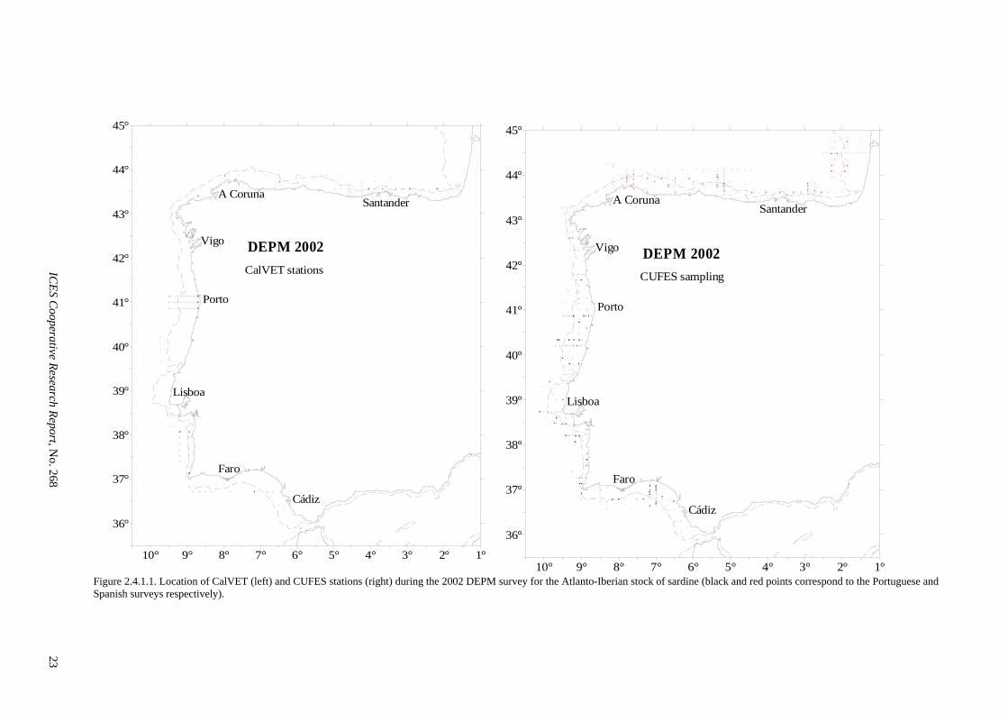
IC
ES Cooperative Research Report, N
o. 268 23
10° 9° 8° 7° 6° 5° 4° 3° 2° 1°
36°
37°
38°
39°
40°
41°
42°
43°
44°
45°
DEPM 2002
Lisboa
Cádiz
Faro
Porto
Santander
Vigo
A Coruna
CalVET stations
10° 9° 8° 7° 6° 5° 4° 3° 2° 1°
36°
37°
38°
39°
40°
41°
42°
43°
44°
45°
DEPM 2002
Lisboa
Cádiz
Faro
Porto
Santander
Vigo
A Coruna
CUFES sampling
Figure 2.4.1.1. Location of CalVET (left) and CUFES stations (right) during the 2002 DEPM survey for the Atlanto-Iberian stock of sardine (black and red points correspond to the Portuguese and Spanish surveys respectively).
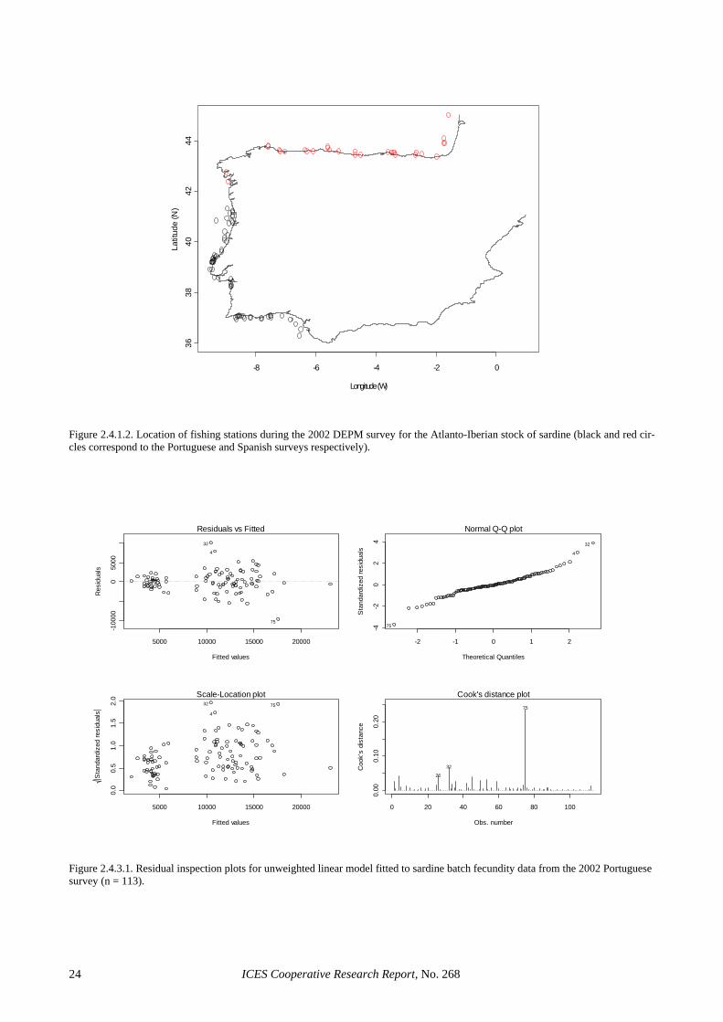
-8 -6 -4 -2 0
3638
4042
44
Longitude (W)
Latit
ude
(N)
Figure 2.4.1.2. Location of fishing stations during the 2002 DEPM survey for the Atlanto-Iberian stock of sardine (black and red cir-cles correspond to the Portuguese and Spanish surveys respectively).
5000 10000 15000 20000
-100
000
5000
Fitted values
Res
idua
ls
Residuals vs Fitted
32
75
4
-2 -1 0 1 2
-4-2
02
4
Theoretical Quantiles
Sta
ndar
dize
d re
sidu
als
Normal Q-Q plot
32
75
4
5000 10000 15000 20000
0.0
0.5
1.0
1.5
2.0
Fitted values
Sta
ndar
dize
d re
sidu
als
Scale-Location plot32 75
4
0 20 40 60 80 100
0.00
0.10
0.20
Obs. number
Coo
k's
dist
ance
Cook's distance plot75
32
26
Figure 2.4.3.1. Residual inspection plots for unweighted linear model fitted to sardine batch fecundity data from the 2002 Portuguese survey (n = 113).
ICES Cooperative Research Report, No. 268 24
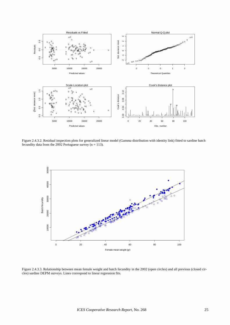
5000 10000 15000 20000
-0.5
0.0
0.5
Predicted values
Res
idua
lsResiduals vs Fitted
32
7588
-2 -1 0 1 2
-2-1
01
23
Theoretical Quantiles
Std
. dev
ianc
e re
sid.
Normal Q-Q plot
32
7588
5000 10000 15000 20000
0.0
0.5
1.0
1.5
Predicted values
Std
. dev
ianc
e re
sid.
Scale-Location plot32
7588
0 20 40 60 80 1000.
000.
040.
080.
12Obs. number
Coo
k's
dist
ance
Cook's distance plot79
75 86
Figure 2.4.3.2. Residual inspection plots for generalized linear model (Gamma distribution with identity link) fitted to sardine batch fecundity data from the 2002 Portuguese survey (n = 113).
0 20 40 60 80 100
1000
020
000
3000
040
000
5000
0
Female mean weight (gr)
Bat
ch fe
cund
ity
Figure 2.4.3.3. Relationship between mean female weight and batch fecundity in the 2002 (open circles) and all previous (closed cir-cles) sardine DEPM surveys. Lines correspond to linear regression fits.
ICES Cooperative Research Report, No. 268 25
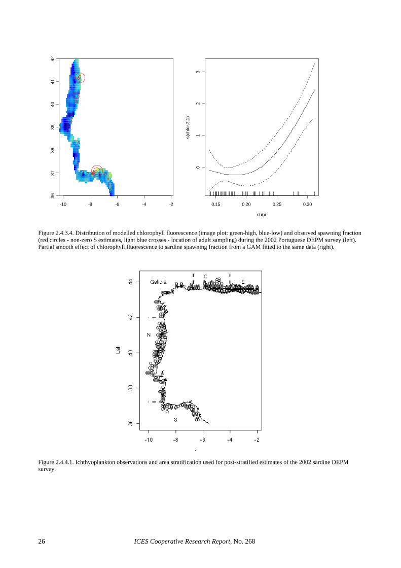
-10 -8 -6 -4 -2
3637
3839
4041
42
++
++
+++++
+++
++++
+ ++ +++ +++++
++
+
+
+++
++++
+++++++++++++
++++
+++++++ ++ ++++ ++
+
+
++
0.15 0.20 0.25 0.300
12
3
chlor
s(ch
lor,2
.1)
Figure 2.4.3.4. Distribution of modelled chlorophyll fluorescence (image plot: green-high, blue-low) and observed spawning fraction (red circles - non-zero S estimates, light blue crosses - location of adult sampling) during the 2002 Portuguese DEPM survey (left). Partial smooth effect of chlorophyll fluorescence to sardine spawning fraction from a GAM fitted to the same data (right).
Figure 2.4.4.1. Ichthyoplankton observations and area stratification used for post-stratified estimates of the 2002 sardine DEPM survey.
ICES Cooperative Research Report, No. 268 26
NANTES
47°
46°
45°
44°
6° 5° 4° 3° 2° 1°
27282930
31323334353637383940414243444546
4748495051525354
10987 252423222120191817161514131211
BIOMAN 20026 - 21 MayR/V INVESTIGADOR
TOTAL area 2002= 56,176 Km²
Spawning area 2002= 35,980 Km²
Figure 2.5.1.1. Anchovy egg/0.1m² distribution found during BIOMAN 2002. Solid line encloses the positive spawning area.
NANTES
47°
46°
45°
44°
6° 5° 4° 3° 2° 1°
27282930
31323334353637383940414243444546
4748495051525354
10987 252423222120191817161514131211
ADULT SAMPLES 2002
11 Commercial purse-seiner samples
26 Thalassa samples
9
14
14
8
16
8
15
16
15
8
14
9
10
10
111111
1212
13 13
14 14
1415
1516
16
16
17
17
17181819
2020
Figure 2.5.1.2. Adult samples obtained by commercial purse-seiners (in blue) and by RV “Thalassa” (in red) for the estimation of anchovy adult parameters in 2002.
ICES Cooperative Research Report, No. 268 27
Exponential Mortality Model - All regions - 2002
Age - Days
Neg
g
3.93 days =90% incubation t
0 1 2 3 4 50
20
40
60
80
100
120
Figure 2.5.2.1. Egg mortality exponential curve fitted to daily cohort egg abundances and mean ages derived from Lo’s ageing method using weighted non linear regression (as traditionally has been done).
0 20 40 60 80 100 120
020
4060
8010
012
0
Bayesian ageing with N(mu=0, sd=1.25)
age (hours)
num
ber o
f egg
s
0 20 40 60 80 100 120
020
4060
8010
012
0
Lo's ageing
age (hours)
num
ber o
f egg
s
Figure 2.5.2.2. Egg mortality exponential curve fitted to the daily cohort egg abundances and mean ages derived from the new Bayes-ian ageing method (left panel) and from the Lo’s ageing method (right panel) using GLMs with negative binomial error distribution and log link.
ICES Cooperative Research Report, No. 268 28
NANTES
47°
46°
45°
44°
6° 5° 4° 3° 2° 1°
27282930
31323334353637383940414243444546
4748495051525354
10987 252423222120191817161514131211
Femal mean weight per haul
20.64 34.87 49.09
Figure 2.5.3.1. Mean female weight distribution in space for Bay of Biscay anchovy in 2002.
ESTRATANEREST
GONAD fw
Bat
ch F
ecun
dity
0 10 20 30 40 500
0.5
1
1.5
2
2.5
3(X 10000)
Figure 2.5.3.2. Batch fecundity vs. gonad free weight for the hydrated anchovy females. A regression line was fitted separately to each stratum (blue and red lines represent the model fitted to the NE and RE strata respectively). Red points represent the outliers, which were removed for the model fitting.
ICES Cooperative Research Report, No. 268 29
Plot of Fitted Model
Wsingonada
Bat
chFe
cund
ity
0 10 20 30 40 500
0.5
1
1.5
2
2.5
3(X 10000)
Figure 2.5.3.3. Batch fecundity vs. gonad free weight for the hydrated anchovy females. Regression line fitted to all the data, assuming that there was no difference between strata. Red points represent the outliers, which were removed for the model fitting.
0
20,000
40,000
60,000
80,000
100,000
120,000
140,000
1987 1988 1989 1990 1991 1992 1993 1994 1995 1996 1997 1998 1999 2000 2001 2002
tonn
es
Figure 2.5.4.1. Series of biomass estimates (tonnes) for the Bay of Biscay anchovy since 1987. Most of them are full DEPM esti-mates, except in 1996, 1999 and 2000, which were deduced indirectly from the relationship of biomass with the spawning area and P0.
ICES Cooperative Research Report, No. 268 30
3 GAMS in DEPM estimation
This section is dedicated to the use of generalized addi-tive models (GAMs) in DEPM estimation. Section 3.1 summarizes aspects of modelling that have received par-ticular attention during the recent EU project on GAMs and Section 3.2 briefly describes the most important methodological innovations resulting from this project. Section 3.3 demonstrates the use of GAMs in the estima-tion of egg production and compares GAM-based with traditional estimates for sardine and anchovy. Section 3.4 extends, for the first time, the application of GAMs to the estimation of adult DEPM parameters and spawning-stock biomass, demonstrating the potential of this method to provide more precise and informative esti-mates. Finally, Section 3.5 describes the current position of the group in relation to the use of GAMs in DEPM es-timation and identifies the additional work necessary to permit a final evaluation on whether GAMs can safely substitute the traditional estimators in routine DEPM ap-plications for sardine and anchovy in the future.
3.1 Introduction GAMs have been shown to be a promising tool for mod-elling egg distribution and estimating egg abundance (e.g. Borchers et al., 1997; Stratoudakis et al., 2003), but several methodological problems remained to be solved prior to the use of the method in the estimation of daily egg production (Bernal, 1999; ICES, 2002). Most of these problems, particularly for sardine and anchovy, have been recently addressed as part of the EU project “Using environmental variables with improved DEPM methods to consolidate the series of sardine and anchovy estimates” (EU Study 99/080). The issues improved dur-ing this project were: • performing model selection using GAMs – previ-
ously this was done on a relatively ad hoc basis with elements of subjectivity;
• modelling in a co-ordinate independent way in a GAM (the model should be insensitive to changes in co-ordinate system);
• modelling interactions in a GAM framework (the crucial issue here is how to scale covariates relative to each other);
• performing inference with GAM models;
• dealing with the over dispersion commonly encoun-tered in egg survey data;
• modelling simultaneously spawning and mortality rates within a GAM framework;
• ensuring stability of models with “difficult” data (many zeros, etc.);
• making the developments easily available to users.
Several members of the SGSBSA participated in the above project, thus the methodological improvements, as well as the necessary software and training in the use of
the new tools have been immediately incorporated to the Study Group. Most of the above issues required a change in the basic statistical methodology applied in GAM es-timation, and the associated improvements are readily applicable to any situation in which GAMs are used. On the other hand, modelling simultaneously egg production and mortality is a problem specific to DEPM and for that several statistical improvements, new data acquisition and new analysis of existing data were performed, both during the above-mentioned EU project and afterwards by the Study Group members.
A simplified general formula of the GAM to be ap-plied for egg production estimation can be expressed as:
E [ Ni ] = g-1 (offset + s ( x1 , by = P0 ) + s ( x2 , by = age )) , where:
Ni = number of eggs in a daily cohort i; g-1 = the inverse of the link function, i.e., the function that makes the relationship between the response and the predictor linear (e.g., logarithm in the case of Poisson); P0 = daily egg production; age = mean age of eggs in daily cohort i; s ( x1 , by = P0 ) = the smooth function that de-scribes the relationship between egg production (on a log scale) and the set of covariates x1 ( for example s (Lat,Long, by = P0) ); s ( x2 , by = age ) = the smooth function that de-scribes the relationship between egg mortality and the set of covariates x2 ( for example s (Depth, by = age) ).
Estimates of age and Ni can be obtained directly from the samples, using an ageing procedure (Section 3.2.1). The offset is a fixed parameter that accounts for differences in sampling size (i.e., volume of water filtered or effec-tive surface sampled). Also, an error structure (which can differ from normal distribution) has to be chosen. The “wiggliness” of the smooth functions used is automati-cally chosen by the new GAM software using General Cross-validation (Section 3.2.3). Nevertheless, the set of covariates used for explaining egg production and mor-tality rates is to be chosen by the scientist, based on the knowledge of the species and the characteristics of the spawning area. Also, whether covariates should enter the equation as univariate (for example, s (Lat, by= P0) + s (Long, by = P0) ) or higher dimension smoothers (for ex-ample, s (Lat , Long, by = P0) ) has to be chosen by the scientist. A brief description of the methods used to es-timate egg production using GAMs is detailed in Sec-tions 3.2.1 to 3.2.5 below.
3.2 Methodology
3.2.1 Egg ageing Estimating egg production in fish species that show fast egg development rates, such as sardines and anchovies, requires estimates of egg mortality in order to use infor-mation from all egg stages. To do so, traditionally eggs are aggregated into cohorts taking into account their ages, and an egg mortality curve is fitted to the abun-
ICES Cooperative Research Report, No. 268 31
dance of daily cohorts given their mean age (e.g., Piquelle and Stauffer, 1985). As only egg stages, and not ages, are observed in the samples, a number of ageing procedures for staged eggs is available in the literature (e.g., Lo, 1985, Bernal et al., 2001). Within the GAM project, and building from the work of Bernal et al. (2001), an innovative and statistically sound ageing pro-cedure was developed and integrated within the GAM analysis of DEPM. The new ageing method is based on the same information traditionally used to age sardine and anchovy eggs, i.e.: • Information from the survey: egg abundance by
stage, sampling time, and environmental conditions affecting the development rate of the egg (usually temperature);
• Information from incubation experiments: the evo-lution of egg stages as their age increases for a given temperature;
• Information from observations on the reproductive biology of the species: distribution of spawning ac-tivity throughout the day.
The evolution of development stages mainly depends on temperature (e.g., review by Pépin, 1991), and to a lower degree on other parameters (see Section 4.2.5). Informa-tion on the rate of egg development as a function of stage and temperature is acquired from incubation experi-ments, in which eggs are reared in a number of tubes or tanks, maintained at a know and constant temperature, and from which samples are drawn periodically. The output from an incubation experiment is treated in the new ageing procedure as a multinomial process in which the probability of staying at a given stage or moving to the next depends both on the (known) age of the egg and on the incubation temperature. Thus, from the output of the incubation experiment we obtain p(s|a,T), the prob-ability of being at stage given age and temperature.
When a fish species shows daily spawning synchro-nicity (the case of sardine and anchovy, see Section 4.2.4), the information on the distribution of spawning activity throughout the day affects the ageing process. If spawning only occurs at certain times, eggs can only have certain ages given the elapsed time between spawn-ing and observation (sampling). In an extreme case, if spawning is perfectly synchronous (eggs are spawned at say, midnight), and development up to hatching lasts only for a day, the observed eggs can only have exactly the elapsed time between midnight and the time they are sampled. If egg development lasts for more than one days, then the approximate mean age observed in the in-cubation experiment can be used to decide at which mid-night it was released, and then just use the elapsed time between the spawning event and the survey time to at-tribute the exact age. In reality, spawning synchronicity information can be formalised as a probability density function (pdf) of age given survey time; ft (a | τ). An ad-ditional, recent, discovery is that mortality should be used to properly age eggs, due to the fact that older eggs are less probable to find, and so, when different daily co-horts can be allocated to an egg, it is more probable that it is younger than older.
Using the information described above and Bayes’ Theorem, it is possible to obtain the distribution of ages given the information obtained in the survey (egg stage, temperature and sampling time):
),|()|(),,|(ˆ TaspafTsap t ττ ∝ and, thus, assign an age to every staged egg by sampling from the posterior distribution ),,|(ˆ Tsap τ or classify eggs in cohorts using the posterior distribution directly. The new ageing procedure has a number of advantages in relation to the previous methods, both in relation to the way that incubation data are modelled, as well as in the actual assignment of ages. In relation to the incubation model: • The new model is clearly described and has a sound
statistical justification. This is a difference with re-spect to the different implementations of Lo’s method, which:
− although easy to implement, allocates random-ness to the wrong variable (age, which in reality is fixed and decided by the researcher);
− it is composed of two different models, one of mean age and another of stage duration. Estima-tion of mean age is not well documented in the different implementations (e.g., Miranda et al., 1990, Motos, 1994), and sometimes is either wrongly described or implemented. The as-sumed model for stage duration also varies in the different implementations of Lo’s method, and again assumptions are not clearly described (i.e., in Motos, 1994 or Miranda et al., 1990);
• The new model has the properties of any other like-lihood method, including asymptotic unbiasedness and efficiency, as well as making easy the compari-son with other likelihood models.
• The uncertainty of the data from the incubation ex-periment is incorporated through the multinomial model.
In relation to the assignment of ages, the advantages of the new ageing model are: • It allows for the inclusion of knowledge on the daily
spawning synchronicity in as complex a way as the data at hand permit/justify;
• It has the potential of including prior distributions of other variables that can affect egg development, and thus the age of an egg at a given stage of develop-ment;
• The posterior distribution of ages has the uncer-tainty of both the incubation experiment and the as-sumed spawning synchronicity built in, and these can be easily accounted for in any subsequent esti-mation that includes age (e.g., the egg mortality curve). Also, the posterior distribution of ages can be used directly to allocate eggs into daily cohorts.
ICES Cooperative Research Report, No. 268 32
Differences between the multinomial and Lo’s model of incubation data, and between the Bayesian and Lo’s age-ing method, and how these affect estimation of egg pro-duction are further investigated in Sections 4.2.2 and 4.2.5 respectively.
3.2.2 Sea area and survey limits estimation Ideally, for design-based inference (which is the form of inference traditionally used in DEPM applications), the survey region should be defined before applying the de-sign. In practice, the design of such surveys is somewhat adaptive, with sampling effort continuing offshore (on transects perpendicular to the coast) until eggs are suffi-ciently sparse to meet some cut-off criterion (see Sec-tions 2.4.1 and 2.5.1 for decisions in recent sardine and anchovy surveys respectively). Design-based analysis of these surveys allocates non-overlapping areas to each sample point (plankton haul) and the survey region is considered to be the region defined by the sum of these areas. This constitutes something like a systematic de-sign without a random start point, which is not an ideal design, but with the intense coverage of points that these surveys achieve it approximates satisfactorily simple random sampling (Smith and Hewitt, 1985).
For GAM-based analysis, a survey region whose boundary is clearly and unambiguously defined is needed in order to predict from the model only on points within the survey area and to avoid extrapolations. Several is-sues on how best to define the inner (inshore) and outer (offshore) limits of the survey area were discussed by the Study Group members and within the EU GAMs project. Assumptions and protocols to define the survey area were unified and a software to semi-automatically define survey areas and limits was produced within the project. The main characteristics of this software are described in Section 3.2.5, while the main decisions on how to define the survey area are summarized below: • Inner (inshore) limits are defined by a smooth ver-
sion of the coastline. This is to avoid extrapolation to unsampled inlets like estuaries or Rias (e.g., in the North-West corner of the Iberian Peninsula);
• Outer (offshore) limits are defined by the outermost survey points of each transect, but adding an extra distance equal to half the distance between survey points in that transect;
• Limits on the start and end of the survey (west and east limits of the survey if the transect are vertical or north and south limits if transects are horizontal) are defined using the position of the outer transects, but adding an extra distance equal to half the distance between transects.
Knowing the exact area represented by a sampling point (or any other point on which prediction takes place) is also important, both for traditional and GAM-based es-timation of egg production. Egg production is measured in units of number of eggs per m2 per day, thus the sur-face sea area represented by each point is needed to ob-tain the estimate of total daily egg production within the survey area. Once more, it is crucial not to extrapolate
outside the survey area and to estimate as precisely as possible the exact area associated to each point, particu-larly in points near the coastline where imprecise estima-tion could lead to extrapolation on land. Estimation of the area represented by each point within the survey area should consider the distance from the point to any of the surrounding points and to the survey limits, so the area represented by each point are never overlapping, and the sum of area represented by all points within the survey area is equal to the total surveyed area. Specific software that automatically calculates the area represented by each point on a regular or an irregular grid along the survey area was created within the GAM project, and its charac-teristics are defined in Section 3.2.5.
3.2.3 Model fitting and selection Within the GAM project, an integrated flexible frame-work for GAM fitting using penalized regression splines (e.g., Wahba, 1980; Parker and Rice, 1985; Eilers and Marx, 1996) was developed. The main aspects of the new framework are: 1) Integrated smoothness selection via GCV (General
Cross-Validation) or unbiased risk estimation (effec-tively AIC);
2) Optimal low rank representation of model component smooth functions of arbitrary numbers of covariates;
3) A rigorous approach to interval estimation based on a Bayesian model of the smoothing process;
4) Extension of the generalized additive model to in-clude “multiplicative offsets” for smooth terms;
5) An efficient approach for using a negative binomial error model with this GAM framework;
6) Development of optimally stable, numerically effi-cient methods for fitting and GCV/AIC smoothness selection;
7) The development of a complete modelling package implementing this framework freely available within the R software.
Points 1, 2, 3 and 7 aimed at improving general GAM fit-ting and providing a widely available framework for ap-plications. Point 4 was developed to deal with particular a aspect of the GAM-based estimation of egg production (dealing properly with egg mortality), while points 5 and 6 were developed based on the feedback from the origi-nal applications to the DEPM data, but which are also relevant to the modelling of other data sets. Although Wood (2000 and 2003) describe in detail most of the above points, a brief summary of the main innovations in GAM fitting and model selection are given below: • GAMs using penalized regression splines: GAMs
can be represented by choosing a basis and a “wig-gliness” penalty for each component of the model, using the bases to set up a model matrix and then fitting the model by penalized likelihood maximisa-tion. When choosing the dimension of each basis there is a trade-off between computational effi-
ICES Cooperative Research Report, No. 268 33
ciency and potential flexibility of the smooth term. In addition, construction of a basis for a multi-dimensional smooth terms is non-trivial if the re-gion covered by the data has a complex shape (e.g., coastal waters of the Iberian Peninsula). During the GAM project, a method for constructing optimal low rank smoothers, termed thin plate regression splines, was developed. The technical work in im-proving the statistical background of GAMs is re-ported in detail by Wood (2003), and is used to rep-resent GAMs in the freely available R package mgcv.
• Integrated smoothness selection by GCV/-UBRE/AIC: Given the representation of the GAM fitting problem as a penalized generalized linear modelling problem, the estimation of the degree of smoothness appropriate for each model term be-comes the problem of choosing the appropriate smoothing parameter by which to weight the wig-gliness penalty for each smooth term in the model fit. Gu and Wahba (1991) pioneered the efficient es-timation of multiple smoothing parameters using GCV for a class of rather computationally costly spline models, and in the work preceding the GAM project (Wood, 2000) this approach was extended to problems including GAMs represented using penal-ized regression splines. The software described in Section 2.2.5 implements this approach with par-ticular emphasis to GAMs, and resolves a number of practical problems associated with ensuring that the methods work on real data sets. Special attention to solve specific problems in relation to treat egg survey data in the GAM framework, like the exis-tence of extensive areas of zeros when a log link is used in the model were dealt with and mostly solved in the associated software. Effectively, the software detailed in Section 2.2.5 allows automatic selection of smoothness, although selection of the dimension of the smoothers and which covariates should be in-cluded together in a multidimensional smoother has still to be chosen by the scientist.
3.2.4 Model prediction and variance estimation Predictions from a fitted GAM can be readily obtained using the software described in Section 3.2.5 in either the sampled grid or in any regular grid (see Section 3.2.2). Extrapolation outside the range of the covariates used for the fitting is strongly inadvisable in the GAM frame-work, due to flexible nature of the relationships between the response and the covariates. Thus, special care to avoid extrapolation should be taken (see for example how to solve geographical extrapolation in Section 3.2.2).
Different methods to obtain confidence intervals and variance estimates can be used in the GAM context. On one hand, theoretically well-founded Bayesian confi-dence intervals were developed for the general GAM framework included in the mgcv software. Nevertheless, these methods are not applicable when combining GAM methods for modelling egg production from DEPM sur-veys with simultaneous estimation of egg mortality,
which involves estimates of age. In this case, confidence intervals are estimated by nonparametric bootstrap, using haul as the sampling unit. The bootstrap procedure was modified to include errors in the fitting, as well as errors in the ageing estimation procedure. Also, when spawning biomass estimates from DEPM are obtained using GAMs both for egg production estimate and for adult parameter estimates, the bootstrap procedure can be expanded to include errors in all the parameters that affect the DEPM estimate of SSB (this component of variance estimation is still needed to be incorporated in the depmodel soft-ware). Thus, reliable estimates of variance and confi-dence intervals for spawning biomass can in principle be obtained from a full GAM-based DEPM analysis (see Section 3.4 and 3.5), although this is not currently avail-able.
3.2.5 Software Three packages that allow fitting GAMs in general (mgcv), implement a GAM-based DEPM estimation (depmodel), and solve geographical problems associated to the analysis of DEPM data (geofun) were developed within the EU project on GAMs. The software was de-veloped in the form of add-on packages for the freely available statistical software R (Ihaka and Gentleman, 1996, CRAN: http://cran.r-project.org/). In general, in-stallation and use of these packages is relatively straight-forward and well documented in the CRAN site and the documentation within each package. The packages (which are available at http://ruwpa-st.andrews.ac.uk/depmodel) are briefly described below: mgcv This is the main package to fit GAMs. The main statisti-cal and computational methods used in the package are already published (Wood, 2003) or are in preparation. The package represents a large methodological im-provement in comparison with other available software to fit GAMs, especially in relation to: • Automatic model selection using General Cross-
validation (GCV) or Unbiased Risk Estimation (UBRE)
• Multidimensional smoothers using the thing plate approach (Wood, 2003)
• Efficient and robust model fitting procedure. It al-lows also fitting over-dispersed data using the nega-tive binomial distribution.
depmodel This package allows GAM-based DEPM analysis and es-timation, including functions for: • Fitting egg incubation models using a flexible ex-
tended continuation-ratio multinomial model (see Section 3.2.1);
• Assigning ages to staged eggs using a new Bayesian ageing method, that relies on the multinomial incu-bation model and a probability density function of
ICES Cooperative Research Report, No. 268 34
spawning activity throughout the day (see Section 3.2.1);
• Classifying eggs in cohorts and estimating cohort abundance and mean cohort age;
• Fitting GAM-based models of egg production, using the general formula shown in Section 3.1.
• Obtaining non-parametric bootstrap estimates of egg production, with uncertainty due to ageing in-corporated.
Functions to obtain summary statistics for the models de-scribed above, as well as functions to plot the results are also included in the package. Some additional improve-ments of the GAM-based DEPM analysis, like including adult parameter variability in the variance estimation us-ing non-parametric bootstrap, or performing a full GAM-based SSB estimation using DEPM are still not included in the actual version of depmodel. geofun The geofun package is designed to modify spatial data for appropriate use in spatial modelling (e.g., using GAMs) and provides some useful functions to repre-sent/map model outputs. Its main functions are to: • Transform pairs of spatial variables (usually Lati-
tude and Longitude) into distances along a given reference line (e.g., the coast line or a selected iso-bath) and perpendicular to it;
• Find the limits of a survey and detect points of any given grid that are within the survey limits;
• Estimate the area represented by each point of a grid (regular or irregular) within the survey limits using Dirichlet tessellation;
• Estimate the area represented by the points located on the edge of the survey, according to the criteria described in Section 3.2.2;
• Provide functions for plotting the results of a spatial model.
The package has been designed specifically to work with marine coastal surveys, where distance from the coast and distance along the coast may be more informative geographic covariates than latitude and longitude. Also, extrapolation to areas on the coast should be avoided, and thus if predictions in points near the coast should be made, point area estimates should be corrected to avoid extrapolation on land. It should be noted that point area is computed by calls to external packages (spatstat and deldir packages available at CRAN) that use Dirichlet tessellation.
3.3 Application to sardine and anchovy DEPM surveys
This section summarizes the methodology and main re-sults from the fitting of GAMs to sardine (Section 3.3.1) and anchovy (Section 3.3.2) eggs from DEPM surveys (see survey details in Section 2). GAM-based estimates
of egg production (and their CV) are compared to those obtained under the traditional estimator (Picquelle and Stauffer, 1985) to evaluate the performance of GAMs in terms of bias and precision.
3.3.1 Sardine The four Iberian DEPM ichthyoplankton surveys for sar-dine (1988, 1997, 1999 and 2002) and a Spanish ich-thyoplankton survey (1990) were used to estimate the daily egg production and mortality in the Atlanto-Iberian stock of sardine using GAMs. Eggs at stage of develop-ment were transformed into daily cohort densities ac-cording to the procedure described in Section 3.2.1 for age assignment that relies on data from an incubation ex-periment (see Section 4.2.2.2) and an assumed daily probability density function of spawning (~N(19,1), but also see Section 4.2.4). Daily egg cohort abundance was modelled as a function of spatial and environmental vari-ables, using a GAM with an over-dispersed Poisson error distribution and a log link. The following variables (ab-breviation used in the remainder appears in brackets) were considered in the model fitted to each survey: • Latitude (Lat): Observed latitude (North, in hun-
dredths of a degree) in a haul (range 35.97 – 44.32);
• Longitude (Long): Observed longitude (west, in hundredths of a degree) in a haul (range 1.88 to 10.34);
• Distance along the coast (Along): from a fixed point on the coast (42o N, close to the northern Portu-guese/Spanish border): The distance is estimated along the coastline (range -1007.9 to 815.8 km, with positive values in Spanish surveys);
• Perpendicular distance (Perp): from the coast: Esti-mated distance of survey stations from closest point to the coast (range 0.5 to 105.6 km);
• Depth (Depth): Fitted bottom depth (in metres) in a haul (range 8 to 7041 m). Fitted values (very flexi-ble spatial GAM to log-transformed depth observa-tions from all surveys; 600 fitted degrees of free-dom, 96.4% of total deviance explained) were used to avoid problems with incorrect/unknown survey observations and to obtain estimates on a regular grid of points within the survey area;
• Temperature (Temp): Fitted water temperature (in decimal degrees C) at near surface waters (5–10 m) in each haul (range 10.9 to 19.3o C). Fitted values (very flexible spatial GAM to temperature observa-tions from each survey; 400 fitted degrees of free-dom, more than 97% of deviance explained in each survey) were used for the reasons explained above;
• Effective area (Efarea): The effective area of the sampler (in m2). This is 0.05 m2 when the CalVET is towed vertically, but variable when towing devi-ates from the vertical due to currents, bad weather, etc. (see ICES, 2002 for method of estimation in these cases).
ICES Cooperative Research Report, No. 268 35
The first four variables provide (in pairs) unique infor-mation for the location of each haul (spatial variables), while depth and temperature provide information about the associated habitat (environmental variables). The two pairs of spatial variables and the pair of environmental variables were used as bivariate smooth functions in the original model fitting. When necessary, variables within a pair were re-scaled to approximate anisotropic interac-tion effects (in the case of the Along:Perp pair, Along was divided by the ratio of the range of the two vari-ables). Further, depth observations were highly right skewed, so log-transformed values were used instead, while the natural logarithm of Efarea was used as an off-set variable to standardise density observations per unit area.
Original models for each DEPM survey were fitted according to the following rules: • Do not allow for spatial variation in mortality;
• Do not include in the same model the two pairs of spatial variables (start with Lat:Long);
• Include a bivariate smooth function of environ-mental variables;
• Do not allow for more than 60 df in bivariate spatial smooths;
• Include the logarithm of Efarea as an offset vari-able.
The best model was chosen based on the GCV score (Wood, 2000) among competing models that converged, according to the following procedure: • Switch pair of spatial variables;
• Test for significance of environmental pair interac-tion;
• Test for significance of univariate environmental ef-fects (if applicable).
Final predictions were performed on a regular grid, as it facilitated image plots and estimation within sub-areas of the stock that are more comparable across years. Vari-ance and confidence intervals for egg production were calculated using a non-parametric bootstrap procedure with haul as the sampling unit. Estimation was based on re-sampling with replacement from the original set of in-cubation and survey data, refitting the original model and repeating the whole process a large number of times (>1000 for each model). Estimates were separated for models fitted to resamples of both survey and incubation data or of survey data only (the difference between the two giving an indication of the variation due to ageing).
Table 3.3.1.1 summarises the model selected for the estimation of sardine daily egg production and mortality in each Iberian DEPM survey. Given that the flexibility of the fitted GAMs was restricted to maintain compara-bility with the traditional estimation, the resulting models led to relatively low percentages of explained deviance. Overall, the explained deviance ranged from 43–60%, with indication of a large over-dispersion (scale parame-ter estimates around or beyond 10). It is also worth not-
ing that in the first three surveys estimates of the mortal-ity parameter are highly significant and consistent among them in indicating hourly mortality rates in the order of 1.5–2%. This is not the case in the latter surveys (when a two months gap is introduced between the onset of the two national surveys), where estimates of mortality are non-significant (1999) or plainly unrealistic (2002). Fi-nally, inspection of standard diagnostic plots indicated the presence of some extreme outliers and a generally poor relation between fitted and observed values.
Figure 3.3.1.1 shows the distribution of bootstrap es-timates of sardine egg production after the removal of some large outliers (estimates more than 3 standard de-viations larger than the bootstrap mean). Inspection of the data sets and models that led to these large outliers (that correspond to 0.4% – 1% of the bootstrap sample in each year) suggest that these can occur when observa-tions with influential values of explanatory variables are omitted in a bootstrap replicate, causing the density sur-face to assume unrealistic shapes. Final estimates of co-efficients of variation (CVs) were based on the bootstrap datasets after the elimination of these large outliers, al-though estimates using all bootstrap re-samples are also tabulated to facilitate comparisons (Table 3.3.1.2). Table 3.3.1.2 also shows some evidence of positive bootstrap bias (in the order of 5–10%), but the estimated CVs are robust to this bias and provide a reasonable basis for es-timating 95% confidence intervals (CIs) assuming a log-normal distribution. Although Figure 3.3.1.1 suggests that there is little difference between assuming a normal or a log-normal distribution for the estimation of CIs, the latter distribution was preferred given that it led to CIs that were generally closer to those based on the bootstrap percentiles.
Table 3.3.1.3 shows the traditional and GAM-based estimates of egg production together with the estimated CVs. Figure 3.3.1.2 provides the same information but with 95% confidence intervals (CIs) plotted instead. CIs are calculated from the tabulated CVs, assuming a nor-mal distribution for the traditional estimates and a log-normal for the GAM-based ones. Overall, point estimates of the two methods are satisfactorily close, with the larg-est relative discrepancy being 18% of the traditional es-timate (1997 survey). A 15% difference is also observed in 1999, but this is justified by the fact that in the GAM method were also used additional data (a second leg of the Spanish survey in the Cantabrian Sea and an ex-tremely high observation from southern Portugal) that were excluded from the traditional estimation (ICES 2002). Based on these results, it seems reasonable to suggest that, despite the large methodological differences between the two estimators (in ageing staged eggs, calcu-lating the sea area associated to a survey point, etc.), point estimates obtained by the two methods are compa-rable and describe a very similar temporal pattern. Also, as demonstrated by the 1990 survey, the two methods perform similarly irrespectively whether the entire Ibe-rian peninsula or just national waters are considered in estimation.
In relation to the precision of the egg production es-timates, the results presented in Table 3.3.1.3 and Figure 3.3.1.2 show that in the three years that identical data sets were used for traditional and GAM-based estima-
ICES Cooperative Research Report, No. 268 36
tion, the latter led to a reduction between 5 and 12% in the estimated CV. This improvement is obtained despite the fact that the GAM-based method also incorporates variation due to the ageing procedure (which in these surveys contributes up to 1% in the tabulated CV) and using simultaneously the data from the two national sur-veys (it is likely that fitting separate models to the two national surveys could lead to an additional improvement in precision, but boundary effects could make distribu-tion plots less useful). In 1999, where the data used by the two methods differ, the GAM method provided an estimate of CV higher by 5% than the traditional. Al-though it is possible that model choice was inadequate for that year, there is no doubt that the inclusion of the highest density ever observed for sardine during DEPM surveys in a CalVET tow (>700 eggs) contributed to this lower (but more realistic given the data) precision.
Figure 3.3.1.3 shows the fitted egg production in comparison with the observed egg abundance in each of the four Iberian DEPM surveys for sardine. These graphs show that the fitted models capture adequately the main features of sardine egg distribution in each DEPM sur-vey. They also permit a synthetic view of the changes in sardine egg distribution over the Iberian Peninsula along the study period, which complements earlier work on sardine spawning areas from GAMs with a binomial er-ror distribution (Bernal, 1999; Stratoudakis et al., 2003); in 1988, more than half of the total production occurred in the northwestern and northern Spanish coast. Ten years later (1997) the situation had dramatically changed, with Galicia and western Cantabrian being practically void of sardine spawning activity. This coincided with a retraction of spawning in the northern Portuguese coast, although intense inshore spawning was observed in the southern Iberia (Algarve and Gulf of Cadiz) during that year. By that time, almost 70% of the total spawning ac-tivity had shifted to the Portuguese waters and the Gulf of Cadiz. The same general pattern was observed in 1999, when more than 90% of the total spawning activity took place in Portuguese waters and the Gulf of Cadiz. In that survey it should be noted the moderate recuperation of spawning in the northern Portuguese coast and the ap-pearance of spectacularly high egg densities in the mid-shelf of the Gulf of Cadiz. The situation seems to be re-verted in 2002 (with a more notable recuperation in northern Portugal), but the low egg production in south-ern Iberia lead to the lowest estimate within the existing series.
3.3.2 Anchovy For the Bay of Biscay anchovy, GAMs for estimating daily egg production and mortality rate were applied to the 1996–1999 egg surveys. The explanatory variables available, with their correspondent abbreviations in brackets, were the following: • Latitude (Lat): Observed latitude (North, in decimal
degrees) in survey stations, ranging from 43ºN to 47ºN.
• Longitude (Long): Observed longitude (west, in decimal degrees) in survey stations, ranging from 1ºW to 5ºW.
• Distance along the coast (Alongdist): Distance (in km) along the coast from a fixed coast point (8.48ºW, 43.37ºN) to the coastline point closest to the survey station.
• Perpendicular distance from the coast (Perpdist): Distance (in km) of the survey station from the clos-est point in the coast.
• Depth (Depth): Fitted bottom depth (in metres) ranging from 15 to 3800 m.
• Temperature (Temp): Fitted water temperature (in degrees C) at 10 meters depth in survey stations, ranging from 13 to 18.6. Assuming that the spawn-ing mainly occurs at 10 m depth, this temperature was considered as the incubation temperature and was used for assigning ages to staged eggs.
• Sst (Sst): Fitted sea surface temperature (in degrees C) in survey stations, ranging from 13.7ºC to 19.6ºC.
• Sss (Sss): Fitted sea surface salinity (in PSU – prac-tical salinity units) in survey stations, ranging from 30 to 36.56 psu.
• Effective area (Efarea): Sea surface area corre-sponding to the volume of water filtered by the ver-tical Pairovet net in each station. This is equivalent to the top area required for a cylinder with a height equal to the actual depth of sampling of the Pairovet in the station to have a volume equal to that actually filtered by the vertical net in the station (according to flow meters). This variable enters the model as an offset in the fitting, to produce egg abundance per surface unit.
Depth, Sst and Sss were not known at locations apart from the survey points, and even in some stations they were not available or reliable due to sampling errors. In order to predict on both the survey grid and on a regular grid within the survey limit avoiding unknown or incor-rect values, different models were fitted to the observed values of these variables each year and fitted values were used instead of the original ones. Depth surface was ob-tained by distance inverse weighted interpolation with a power of 2 and a search ratio of 10 nautical miles, ap-plied to a combination of data from ship echo-sounder readouts during the surveys (1994–1999), data from ETOPO2 global bathymetric model and coastline from GEBCO Global digital atlas. Alternatively, Sst and Sss surfaces for each year were fitted as a function of latitude and longitude using very flexible GAMs with normal er-rors and identity link. Table 3.3.2.1 shows the number of observations (N), the number of knots (k) and the per-centage deviance explained by each of the models for Sst and Sss. The response residuals were less than 0.6ºC and 1 psu for the Sst and Sss models respectively.
The short life span of anchovy makes the level of biomass strongly dependent on the recruitment occurring each year, which at the same time is very variable and
ICES Cooperative Research Report, No. 268 37
dependent on the environmental conditions. Figure 3.3.2.1 shows the egg abundance found in 1996–1999 surveys, together with the environmental situation as de-scribed by sea surface salinity and sea surface tempera-ture. 1997 presented very high salinities over the whole area. Lower salinities (mainly in the area in front of the Gironde River) were found in 1996 and 1998. Especially in 1998 the lower salinity areas were more spread along the French coast and higher temperatures were also en-countered. On the contrary, 1999 showed low salinities and high temperatures across the whole area. Hence, en-vironmental conditions appeared to be indispensable for modelling adequately the egg spatial distribution.
The smooth terms considered for modelling the daily spawning rate were: • s(Long, Lat) for describing the spatial location. Two
bivariate smooths, s(Long, Lat) and s(Alongdist, Perpdist), were available for representing the geo-graphical location of the points. However, it was decided to use only one pair in a given model. Given the “rectangular form” of the Bay of Biscay the differences between both options were minor, but s(Long, Lat) was selected as the more natural one.
• s(Sst.fit, Sss.fit) for describing the environmental situation. Given that Sst and Sss were highly corre-lated, a bivariate smooth was considered.
• s(Log(Depth)). Depth was log transformed due to its skewed distribution.
• s(Log(Depth), Alongdist/87) in order to analyse whether the effect of Depth on the anchovy daily spawning rate distribution changed in space. For ex-ample in the northern Spanish coast the depth gradi-ent is very steep, being the 200 m depth contour line very close to the coast, whereas in the French coast the gradient is smoother, and this could affect the egg distribution. Alongdist was re-scaled (divided by the mean of the ranges ratio) in order to avoid anisotropy problems.
And for the daily mortality rate: • Constant over the whole area, as assumed in the tra-
ditional DEPM.
• s(Long, Lat) for describing daily mortality rate varying very smoothly in space
Models considered and correspondent names are shown in Table 3.3.2.2. All models were fitted using the pack-age depmodel (Section 3.2.5). GAMs with over-dispersed Poisson error distribution and log link were considered. Staged eggs were transformed into daily co-horts using the procedure described in Section 3.2.1, with the multinomial model for the distribution of stage given age and temperature as described in Section 4.2.2.1 and spawning time distribution assumed to be normal with mean at 23 and standard deviation of 1.25 (see Section 4.2.4).
Models m4 and z4 had the lowest GCV score and the largest % deviance explained in all years. Models m4
have a GCV between 8 and 14 and explained between 50 and 60% of the deviance, with large values of the scale parameters indicating over dispersion. The significance and degrees of freedom of the smooth terms were rather consistent from year to year. Same models but allowing z to vary in space (z4), presented very similar GCV but a slightly higher % of deviance explained (between 54 and 65%). Estimates of the daily mortality rate parametric coefficient decreased, although the smoothed mortality term was significant in all the years. Diagnostic plots for these models did not show any important trend, though some outliers were detected. By the time being, and simi-larly to the traditional DEPM, invariant mortality in space was assumed and m4 was selected as the best model for anchovy. Summary statistics for this model are presented in Table 3.3.2.3.
The GAM-based total egg production estimate was computed as the sum of the predicted values on a grid of points within the survey area. In order to avoid the effect of using different sea areas when comparing the GAM based and the traditional estimates, the GAM based esti-mates were computed using three different approaches: a) predicting on the survey grid with the sea area repre-
sented by each station being the same as used in the traditional method.
b) predicting on the survey grid with the sea area repre-sented by each station computed by geofun (Section 3.2.5).
c) predicting on a regular grid (denser than the survey grid) using the sea area computed by geofun.
Table 3.3.2.4 shows the GAM-based total egg production estimates from model m4, together with the traditional DEPM estimates, while Figure 3.3.2.2 provides image and contour plots for the fitted egg production models. Estimates of the variance associated to each of the total egg production estimates in (a) were obtained by non-parametric bootstrap from the original incubation ex-periment and survey data. Estimates for re-sampling only the survey data and of re-sampling both survey and incu-bation data were stored separately, so that the variance associated to the incubation experiment could also be evaluated.
Figure 3.3.2.3 shows distributions of the bootstrapped egg production values after removing the outliers (esti-mates larger than twice the first GAM-based egg produc-tion estimate). Added line shows the density function of a normal distribution with mean and standard deviation taken from the bootstrap sample. The distributions of the bootstrap estimates are quite close to a normal distribu-tion. Table 3.3.2.5 shows % bootstrap bias, computed as the % difference between GAM estimate of egg produc-tion and bootstrap mean, and CV estimates, considering firstly only re-sampling on the survey data and secondly re-sampling on the incubation and survey data. Some evidence of positive bias is observed. CV estimates are similar for including or not re-sampling on the incuba-tion data, suggesting that the incubation experiment did not add much variation to the final egg production esti-mate. Figure 3.3.2.4 shows the daily egg production es-timates given by the traditional DEPM and by the se-
ICES Cooperative Research Report, No. 268 38
lected GAMs, with their correspondent confidence inter-vals computed from the estimated CVs assuming normal distribution. In this case, confidence intervals for GAM-based estimates are larger than those of the traditional method. However, note that the traditional CV estimates seem surprisingly small (as low as 5% in one case), sug-gesting that they might be negatively biased. The GAM method CVs are very plausible, between 13% and 21%, and are more reliable.
3.4 GAMS in adult parameter and biomass esti-mation: a first example
One of the main advantages from the application of GAMs to DEPM estimation is that, given an adequate number of fish samples, its use can be extended to the es-timation of adult parameters and hence the direct model-based estimation of spawning-stock biomass (Borchers et al., 1997). However, unlike eggs (where, for example, around 800 observations are available in each sardine survey in the Iberian Peninsula), adult sampling is al-ways considerably more limited (35–40 adult stations in most years) and in some cases parts of the survey area are not sampled. Here, is presented an exploratory at-tempt to provide GAM-based estimation of spawning biomass for sardine and anchovy using the 2002 survey data.
3.4.1 Sardine Adult sampling in the 2002 Portuguese and Spanish sur-veys was considerably intensified, providing adult pa-rameter estimates from 102 fishing stations (74 in Portu-gal and the Gulf of Cadiz and 28 in Spain). These data (described in Section 2.4) are used here to explore for the first time the application of GAMs to sardine adult pa-rameter and spawning-stock biomass (SSB) estimation. Models were fitted using the explanatory variables listed in 3.3.1 (apart from Efarea). Alongdist and Perpdist were estimated by geofun (Section 3.2.5), while temperature was obtained from the same model that provided fitted sea surface temperatures for the egg data set. Depth in this case refers to observed sampled depth, while addi-tional information (fishing gear, sampling time and sam-ple size) was also available.
A GAM with a binomial error distribution and a logit link was fitted to spawning fraction and sex ratio (with the binomial denominator being the number of histologi-cally observed gonads and the total number of sampled fish respectively). A GAM with a normal error distribu-tion and an identity link was fitted to mean female weight and batch fecundity. In the case of batch fecun-dity, it is natural that the fitted model will be very similar to that for mean weight given that fecundity is a variable derived from female weight. In all cases, only one bivariate set of explanatory variables was considered, aiming to capture the observed spatial structure. Table 3.4.1.1 provides a summary of the model selected for each variable and Figure 3.4.1.1 shows the residual in-spection plots for the mean weight and spawning fraction models respectively. Overall, relatively simple bivariate models seem to have captured adequately the main struc-ture in the 4 adult parameters estimated along Iberia.
To obtain an estimate of SSB, each adult parameter was predicted on the regular grid used for GAM-based estimation of egg production, and the traditional DEPM equation was applied to each grid point. SSB was esti-mated by summing across the grid, leading to an estimate of 466.2 thousand tonnes, of which only 45 (10%) in northern Spain. Figure 3.4.1.2 shows the spatial distribu-tion of the predicted values of sardine spawning fraction and mean weight during the 2002 DEPM survey, both exhibiting strong spatial patterns. Spawning fraction is very low in Portugal, with patches of spawning activity in Cadiz and northern Portugal. In northern Spain, spawning activity is more intense and homogeneous, but with an increasing trend from central to eastern Can-tabria. In mean weight there is a clear latitudinal trend, with fish in the Cantabrian Sea being considerably heav-ier than in western and southern Iberia. There is also evi-dence that first time spawners are concentrated predomi-nantly in the Gulf of Cadiz and in a restricted zone in northern Portugal, which is in good agreement with ex-isting knowledge on sardine recruitment zones.
The use of GAMs for adult parameter and SSB estimation also permits to visualise the distribution of spawning biomass in space. Figure 3.4.1.2 shows the es-timated SSB along Iberia simultaneously with the distri-bution of observed total eggs (left) and the distribution of acoustic energy allocated to sardine (right). Overall, the two surveys seem to provide a reasonably similar re-gional distribution, although in the case of the Portu-guese acoustics fish densities are observed closer to the shore. This most likely reflects the processes of passive offshore egg transport through diffusion and advection, which is often observed in the northern Portuguese coast. Finally, GAMs could also be used in relatively large data sets (probably when merging information from various years) to explore issues related to sampling (e.g., impact of sampling gear and time).
3.4.2 Anchovy For anchovy, adult sampling in 2002 supplied a total of 35 samples (see Section 2.5), allowing a first exploration of GAM fitting to adult anchovy DEPM parameters. The two key adult parameters for DEPM are female weight (W) and spawning fraction (S), since batch fecundity is directly dependent on W (by a linear model) and ex-pected sex ratio in weight can also be inferred from W under the hypothesis of 1:1 sex ratio in numbers. The lat-ter is a hypothesis validated for the Bay of Biscay an-chovy in 1997 and 1998 (Uriarte et al., 1999a). Spawn-ing fraction can be either dependent on W (if age de-pendent) and/or on the environmental conditions (tem-perature, plankton productivity, etc.) in the different spawning areas. Hence, spatial trends in these two pa-rameters can be fitted by a GAM, provided that a suffi-cient number of adult samples is available within the survey area.
Modelling mean female weight (W): GAM fitting to W was based on a simple bivariate smooth of Lat and Long coordinates, assuming a Gaussian error distribution and an identity link function. No environmental covariate was explored. Two GAM models were tested; one based on the default maximum number of knots allowed auto-
ICES Cooperative Research Report, No. 268 39
matically for smoothing by the GAM function in mgcv (max of 30 knots) and a second restricting the maximum number of knots to 10. This comparison was deemed necessary since the former model required 26 degrees of freedom (df) for the fitting of 35 observations. The summary statistics (Table 3.4.2.1) show that the default model explained 99% of the observed spatial variability in mean female weight, while the second (which required 7.4 df) explained 89% of the variability. The potential of bias due to overfitting is evident in the first model, and the second model was considered good enough. Figure 3.4.2.1 shows the standard checking for this later model whereas Figure 3.4.2.2 presents the fitted surface with the observed female mean weight.
Modelling spawning fraction (S): GAM fitting to S was based on a simple bivariate smooth of Lat and Long coordinates, assuming a binomial error distribution, a logit link function and weights (binomial denominator) equal to the number of mature females examined his-tologically per haul. No environmental covariate was ex-plored. Figure 3.4.2.3 shows the standard checking figures of the fitted model for S. This parameter could not be successfully fitted by GAM, with only 2% of the spatial variability being explained and the fitting was not significant (Table 3.4.2.2). Potential relationships with female weight or Depth were explored but also found non-significant, hence S was taken as a random Gaussian variable represented in space by its mean and CV.
Modelling sex ratio (R’): Given that the sex ratio for anchovy is since 1994 assumed to be 1:1 in numbers, the expected sex ratio in weight (R´) can be inferred from Wf and the Wm (mean weight of females and males respec-tively) as follows:
( ) www = R
mf
f
+'
Males have a slightly lower weight than females accord-ing to a fitted linear model (Figure 3.4.2.4).
Modelling batch fecundity (F): Batch fecundity can be directly estimated from the gonad free weight of fe-males by the standard linear relationship fitted in tradi-tional DEPM analysis. However, given the very good fit-ting of GAM to mean weight of females we decided simply to repeat the fitting for F attaining similar good levels of fit.
Modelling egg production (P0): Two different GAMs with Poisson error distribution and log link were fitted to the egg abundances by ages obtained from the egg sur-vey and following the method and software described in Sections 2.1 to 2.3. First model, model 0, considers solely a spatial component for the daily egg production rate, P0, through a bivariate smooth of Latitude and Lon-gitude. Second model, model 1, also includes an envi-ronmental term, a bivariate smooth for Sss and Sst. As in the traditional DEPM, both models assumed constant mortality over the whole survey area. The improvement obtained by including the environmental covariates was noticeable and significant, attaining in total an explana-tion of 64.6 of the original deviance. Summary statistics of the fitted GAMs for P0 estimations are presented in Table 3.4.2.3.
Egg production surface (Figure 3.4.2.5) was obtained by predicting over the regular grid and total egg produc-tion was computed as the sum of the predicted values across the regular grid. In order to obtain an estimate of SSB, each adult parameter was predicted on the regular grid used for the GAM-based estimation of egg produc-tion. Female weight and batch fecundity were obtained by predicting from the correspondent fitted GAMs on the regular grid. Male weight was derived from the female weight predicted surface using the linear model shown in Figure 3.4.2.4. So that sex ratio surface was computed as the proportion of female weight over the total weight in each of the regular grid points. As no spatial structure was found for the spawning fraction, a constant mean surface over the whole area was considered. Then, the to-tal predicted SSB was obtained by first applying the tra-ditional DEPM equation to each grid point, and then summing across the whole area. Table 3.4.2.4 presents the final total egg production and SSB estimates for Bay of Biscay anchovy in 2002 and Figure 3.4.2.6 shows the spatial distribution of SSB.
3.5 Discussions and recommendations Overall, the methods and software developed in the EU project on GAMs provide effective tools for estimating daily egg production, analysing data from incubation ex-periments and estimating the total area of plankton sur-veys and the corresponding repartition among fixed sta-tions in a statistically rigorous manner. They have been shown to yield estimates of egg production that have higher precision than traditional methods, without any evidence of bias. Despite the fact that GAM-based esti-mation of precision is penalized by the consideration of variation due to ageing, reductions in the estimated coef-ficient of variation (CV) by 5–15% were observed in the sardine data to which it was applied. No reductions were observed in the anchovy application, but there is reason to suspect that the traditional CV estimates are nega-tively biased; the new CV estimates are considered more reliable. GAMs can also be an effective means of esti-mating the distribution of adult parameters and spawning biomass within the stock region, avoiding ad-hoc deci-sions on post-stratifications and providing the potential for additional improvements in the precision of the bio-mass estimates. Further, in the case of sardine, the esti-mates of SSB and the spatial distribution of adult pa-rameters and SSB are in good agreement with other sources of information (acoustic surveys) and with exist-ing knowledge on the species dynamics in the Iberian Peninsula.
GAM-based estimation of egg production also has the potential to relax the assumption that egg mortality is constant throughout the survey region and can model egg mortality surfaces and empirical relationships between environmental/oceanographic variables and mortality. Apart from improving estimation, this has the potential to provide useful biological insight to the processes that control pelagic egg mortality, which, together with the improved understanding of the spatial distribution of re-productive parameters, open new perspectives in the study of sardine and anchovy dynamics and its relation to environmental conditions. However, the introduction of
ICES Cooperative Research Report, No. 268 40
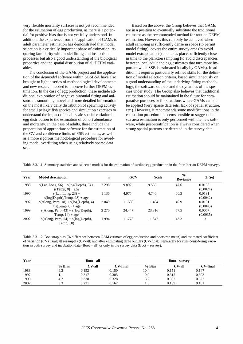
very flexible mortality surfaces is not yet recommended for the estimation of egg production, as there is a poten-tial for positive bias that is not yet fully understood. In addition, the experience from the application of GAMs to adult parameter estimation has demonstrated that model selection is a critically important phase of estimation, re-quiring familiarity with model fitting and inspection processes but also a good understanding of the biological properties and the spatial distribution of all DEPM vari-ables.
Based on the above, the Group believes that GAMs are in a position to eventually substitute the traditional estimator as the recommended method for routine DEPM estimation. However, this can only be achieved when adult sampling is sufficiently dense in space (to permit model fitting), covers the entire survey area (to avoid model extrapolations) and takes place sufficiently close in time to the plankton sampling (to avoid discrepancies between local adult and egg estimates that turn more im-portant when SSB is estimated locally by GAMs). In ad-dition, it requires particularly refined skills for the defini-tion of model selection criteria, based simultaneously on a good understanding of the underlying fitting methodo-logy, the software outputs and the dynamics of the spe-cies under study. The Group also believes that traditional estimation should be maintained in the future for com-parative purposes or for situations where GAMs cannot be applied (very sparse data sets, lack of spatial structure, etc.). However, it recommends some modifications in the estimation procedure: it seems sensible to suggest that sea area estimation is only performed with the new soft-ware, while post-stratification is always considered when strong spatial patterns are detected in the survey data.
The conclusion of the GAMs project and the applica-tion of the depmodel software within SGSBSA have also brought to light a series of methodological developments and new research needed to improve further DEPM es-timation. In the case of egg production, these include ad-ditional exploration of negative binomial fitting and ani-sotropic smoothing, novel and more detailed information on the most likely daily distribution of spawning activity for small pelagic fish species and simulation exercises to understand the impact of small-scale spatial variation in egg distribution to the estimation of cohort abundance and mortality. In the case of adults, these include the preparation of appropriate software for the estimation of the CV and confidence limits of SSB estimates, as well as a more rigorous methodological procedure for avoid-ing model overfitting when using relatively sparse data sets.
Table 3.3.1.1. Summary statistics and selected models for the estimation of sardine egg production in the four Iberian DEPM surveys.
Year Model description n GCV Scale % Deviance Z (se)
1988 s(Lat, Long, 56) + s(log(Depth), 6) + s(Temp, 8) + age
2 298 9.892 9.585 47.6 0.0138 (0.0024)
1990 s(Lat, Long, 23) + s(log(Depth),Temp, 28) + age
1 136 4.975 4.746 60.3 0.0191 (0.0042)
1997 s(Along, Perp, 18) + s(log(Depth), 4) + s(Temp, 8) + age
2 049 11.580 11.404 49.9 0.0131 (0.0045)
1999 s(Along, Perp, 43) + s(log(Depth), Temp, 14) + age
2 270 24.447 23.816 57.5 0.0057 (0.0035)
2002 s(Along, Perp, 54) + s(log(Depth), Temp, 18)
1 994 11.778 11.347 43.2 0
Table 3.3.1.2. Bootstrap bias (% difference between GAM estimate of egg production and bootstrap mean) and estimated coefficient of variation (CV) using all resamples (CV-all) and after eliminating large outliers (CV-final), separately for runs considering varia-tion in both survey and incubation data (Boot – all) or only in the survey data (Boot – survey).
Year Boot - all Boot - survey % Bias CV-all CV-final % Bias CV-all CV-final
1988 9.2 0.152 0.150 10.4 0.151 0.147 1997 1.1 0.317 0.305 0.9 0.312 0.303 1999 4.2 0.338 0.328 3.2 0.332 0.322 2002 3.3 0.221 0.162 1.5 0.189 0.151
ICES Cooperative Research Report, No. 268 41
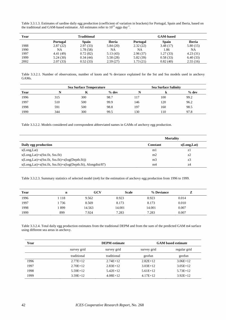
Table 3.3.1.3. Estimates of sardine daily egg production (coefficient of variation in brackets) for Portugal, Spain and Iberia, based on the traditional and GAM-based estimator. All estimates refer to 1012 eggs day-1. Year Traditional GAM-based
Portugal Spain Iberia Portugal Spain Iberia 1988 2.87 (22) 2.97 (33) 5.84 (20) 2.32 (22) 3.48 (17) 5.80 (15) 1990 NA 1.78 (58) NA NA 1.86 NA 1997 4.41 (49) 0.72 (82) 5.13 (43) 2.96 (37) 1.27 (33) 4.23 (31) 1999 5.24 (30) 0.34 (44) 5.58 (28) 5.82 (39) 0.58 (33) 6.40 (33) 2002 2.07 (33) 0.52 (33) 2.59 (27) 1.73 (21) 0.82 (40) 2.55 (16) Table 3.3.2.1. Number of observations, number of knots and % deviance explained for the Sst and Sss models used in anchovy GAMs.
Sea Surface Temperature Sea Surface Salinity Year N K % dev N k % dev 1996 315 300 98.7 117 100 99.2 1997 510 500 99.9 146 120 96.2 1998 591 500 98.8 197 160 98.5 1999 344 300 99.5 130 110 97.8 Table 3.3.2.2. Models considered and correspondent abbreviated names in GAMs of anchovy egg production. Mortality
Daily egg production Constant s(Long,Lat) s(Long,Lat) m1 z1 s(Long,Lat)+s(Sst.fit, Sss.fit) m2 z2 s(Long,Lat)+s(Sst.fit, Sss.fit)+s(log(Depth.fit)) m3 z3 s(Long,Lat)+s(Sst.fit, Sss.fit)+s(log(Depth.fit), Alongdist/87) m4 z4 Table 3.3.2.3. Summary statistics of selected model (m4) for the estimation of anchovy egg production from 1996 to 1999. Year n GCV Scale % Deviance Z
1996 1 118 9.562 8.923 8.923 0.014 1997 1 736 8.569 8.173 8.173 0.010 1998 1 899 14.563 14.001 14.001 0.007 1999 899 7.924 7.283 7.283 0.007 Table 3.3.2.4. Total daily egg production estimates from the traditional DEPM and from the sum of the predicted GAM m4 surface using different sea areas in anchovy.
Year DEPM estimate GAM based estimate
survey grid survey grid survey grid regular grid
traditional traditional geofun geofun 1996 2.77E+12 2.74E+12 2.82E+12 3.06E+12 1997 2.70E+12 2.83E+12 3.03E+12 3.05E+12 1998 5.59E+12 5.42E+12 5.61E+12 5.73E+12 1999 3.59E+12 4.08E+12 4.17E+12 3.92E+12
ICES Cooperative Research Report, No. 268 42
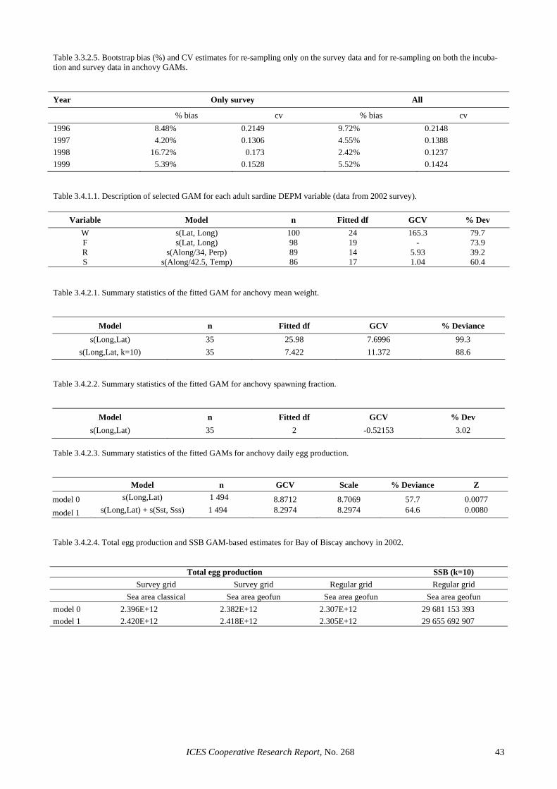
Table 3.3.2.5. Bootstrap bias (%) and CV estimates for re-sampling only on the survey data and for re-sampling on both the incuba-tion and survey data in anchovy GAMs. Year Only survey All
% bias cv % bias cv 1996 8.48% 0.2149 9.72% 0.2148 1997 4.20% 0.1306 4.55% 0.1388 1998 16.72% 0.173 2.42% 0.1237 1999 5.39% 0.1528 5.52% 0.1424 Table 3.4.1.1. Description of selected GAM for each adult sardine DEPM variable (data from 2002 survey).
Variable Model n Fitted df GCV % Dev W s(Lat, Long) 100 24 165.3 79.7 F s(Lat, Long) 98 19 - 73.9 R s(Along/34, Perp) 89 14 5.93 39.2 S s(Along/42.5, Temp) 86 17 1.04 60.4
Table 3.4.2.1. Summary statistics of the fitted GAM for anchovy mean weight.
Model n Fitted df GCV % Deviance s(Long,Lat) 35 25.98 7.6996 99.3
s(Long,Lat, k=10) 35 7.422 11.372 88.6 Table 3.4.2.2. Summary statistics of the fitted GAM for anchovy spawning fraction.
Model n Fitted df GCV % Dev s(Long,Lat) 35 2 -0.52153 3.02
Table 3.4.2.3. Summary statistics of the fitted GAMs for anchovy daily egg production.
Model n GCV Scale % Deviance Z
model 0 s(Long,Lat) 1 494 8.8712 8.7069 57.7 0.0077 model 1 s(Long,Lat) + s(Sst, Sss) 1 494 8.2974 8.2974 64.6 0.0080 Table 3.4.2.4. Total egg production and SSB GAM-based estimates for Bay of Biscay anchovy in 2002.
Total egg production SSB (k=10) Survey grid Survey grid Regular grid Regular grid Sea area classical Sea area geofun Sea area geofun Sea area geofun model 0 2.396E+12 2.382E+12 2.307E+12 29 681 153 393 model 1 2.420E+12 2.418E+12 2.305E+12 29 655 692 907
ICES Cooperative Research Report, No. 268 43
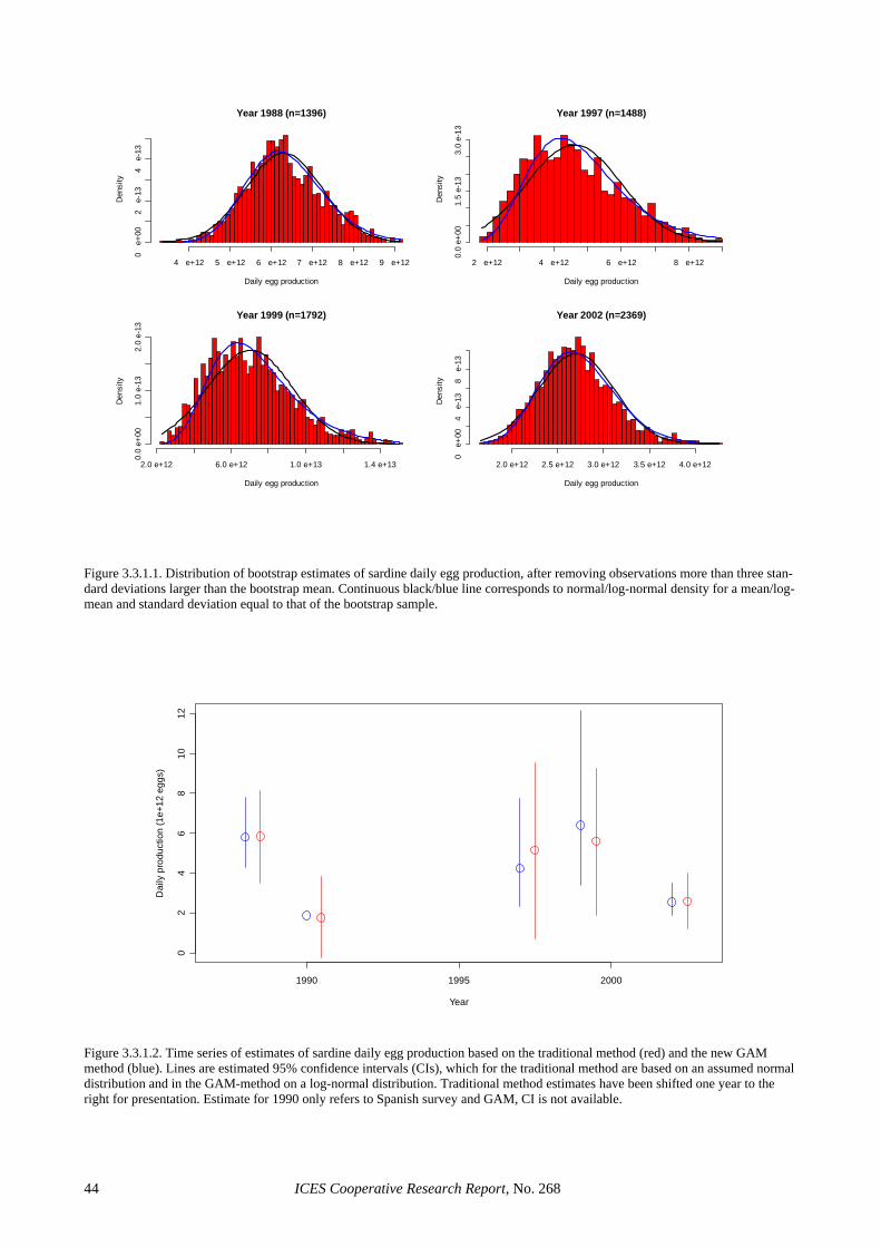
Year 1988 (n=1396)
Daily egg production
Den
sity
4 e+12 5 e+12 6 e+12 7 e+12 8 e+12 9 e+12
0 e
+00
2 e
-13
4 e
-13
Year 1997 (n=1488)
Daily egg production
Den
sity
2 e+12 4 e+12 6 e+12 8 e+12
0.0
e+00
1.5
e-13
3.0
e-13
Year 1999 (n=1792)
Daily egg production
Den
sity
2.0 e+12 6.0 e+12 1.0 e+13 1.4 e+13
0.0
e+00
1.0
e-13
2.0
e-13
Year 2002 (n=2369)
Daily egg production
Den
sity
2.0 e+12 2.5 e+12 3.0 e+12 3.5 e+12 4.0 e+120
e+0
04
e-1
38
e-1
3
Figure 3.3.1.1. Distribution of bootstrap estimates of sardine daily egg production, after removing observations more than three stan-dard deviations larger than the bootstrap mean. Continuous black/blue line corresponds to normal/log-normal density for a mean/log-mean and standard deviation equal to that of the bootstrap sample.
1990 1995 2000
02
46
810
12
Year
Dai
ly p
rodu
ctio
n (1
e+12
egg
s)
Figure 3.3.1.2. Time series of estimates of sardine daily egg production based on the traditional method (red) and the new GAM method (blue). Lines are estimated 95% confidence intervals (CIs), which for the traditional method are based on an assumed normal distribution and in the GAM-method on a log-normal distribution. Traditional method estimates have been shifted one year to the right for presentation. Estimate for 1990 only refers to Spanish survey and GAM, CI is not available.
ICES Cooperative Research Report, No. 268 44
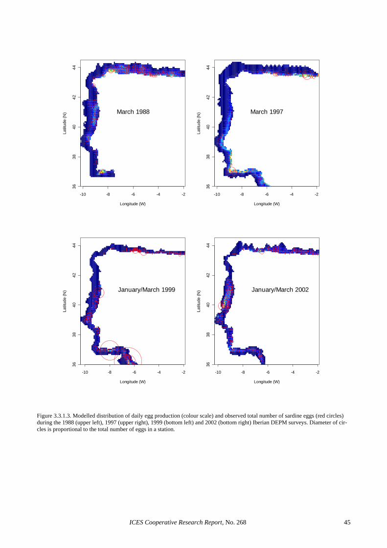
-10 -8 -6 -4 -2
3638
4042
44
Longitude (W)
Latit
ude
(N) March 1988
-10 -8 -6 -4 -2
3638
4042
44Longitude (W)
Latit
ude
(N) March 1997
-10 -8 -6 -4 -2
3638
4042
44
Longitude (W)
Latit
ude
(N) January/March 1999
-10 -8 -6 -4 -2
3638
4042
44
Longitude (W)
Latit
ude
(N) January/March 2002
Figure 3.3.1.3. Modelled distribution of daily egg production (colour scale) and observed total number of sardine eggs (red circles) during the 1988 (upper left), 1997 (upper right), 1999 (bottom left) and 2002 (bottom right) Iberian DEPM surveys. Diameter of cir-cles is proportional to the total number of eggs in a station.
ICES Cooperative Research Report, No. 268 45
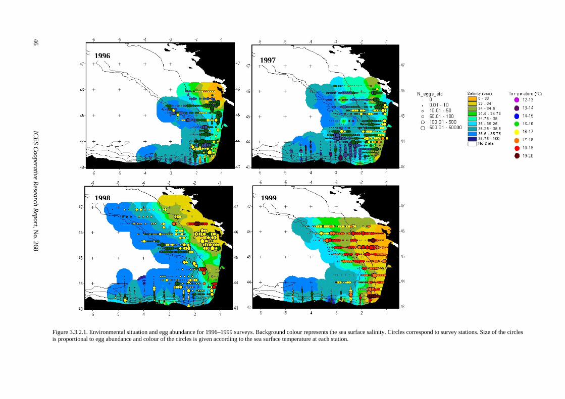
46 IC
ES Cooperative Research Report, N
o. 268
1996 1997
1998 1999
Figure 3.3.2.1. Environmental situation and egg abundance for 1996–1999 surveys. Background colour represents the sea surface salinity. Circles correspond to survey stations. Size of the circles is proportional to egg abundance and colour of the circles is given according to the sea surface temperature at each station.
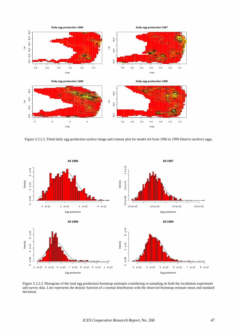
-4.0 -3.5 -3.0 -2.5 -2.0 -1.5
43.5
44.0
44.5
45.0
45.5
46.0
Daily egg production 1996
Long
Lat
-4.5 -4.0 -3.5 -3.0 -2.5 -2.0 -1.5
43.5
44.5
45.5
Daily egg production 1997
Long
Lat
-5 -4 -3 -2
43.5
44.5
45.5
46.5
Daily egg production 1998
Long
Lat
-4.5 -4.0 -3.5 -3.0 -2.5 -2.0 -1.5
43.5
44.5
45.5
Daily egg production 1999
Long
Lat
Figure 3.3.2.2. Fitted daily egg production surface image and contour plot for model m4 from 1996 to 1999 fitted to anchovy eggs.
All 1996
Egg production
Den
sity
2 e+12 3 e+12 4 e+12 5 e+12
0 e
+00
3 e
-13
6 e
-13
All 1997
Egg production
Den
sity
2.0 e+12 3.0 e+12 4.0 e+12 5.0 e+12
0.0
e+00
6.0
e-13
1.2
e-12
All 1998
Egg production
Den
sity
4 e+12 5 e+12 6 e+12 7 e+12 8 e+12 9 e+12 1 e+13
0 e
+00
4 e
-13
8 e
-13
All 1999
Egg production
Den
sity
3 e+12 4 e+12 5 e+12 6 e+12 7 e+12 8 e+12
0 e
+00
4 e
-13
8 e
-13
Figure 3.3.2.3. Histogram of the total egg production bootstrap estimates considering re-sampling on both the incubation experiment and survey data. Line represents the density function of a normal distribution with the observed bootstrap estimate mean and standard deviation.
ICES Cooperative Research Report, No. 268 47
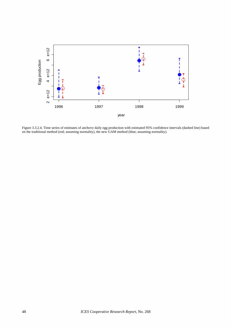
2 e
+12
4 e
+12
6 e
+12
year
Egg
pro
duct
ion
- -
--
--
--
1996 1997 1998 1999
- -
-
--
-
-
-
Figure 3.3.2.4. Time series of estimates of anchovy daily egg production with estimated 95% confidence intervals (dashed line) based on the traditional method (red; assuming normality), the new GAM method (blue; assuming normality).
ICES Cooperative Research Report, No. 268 48
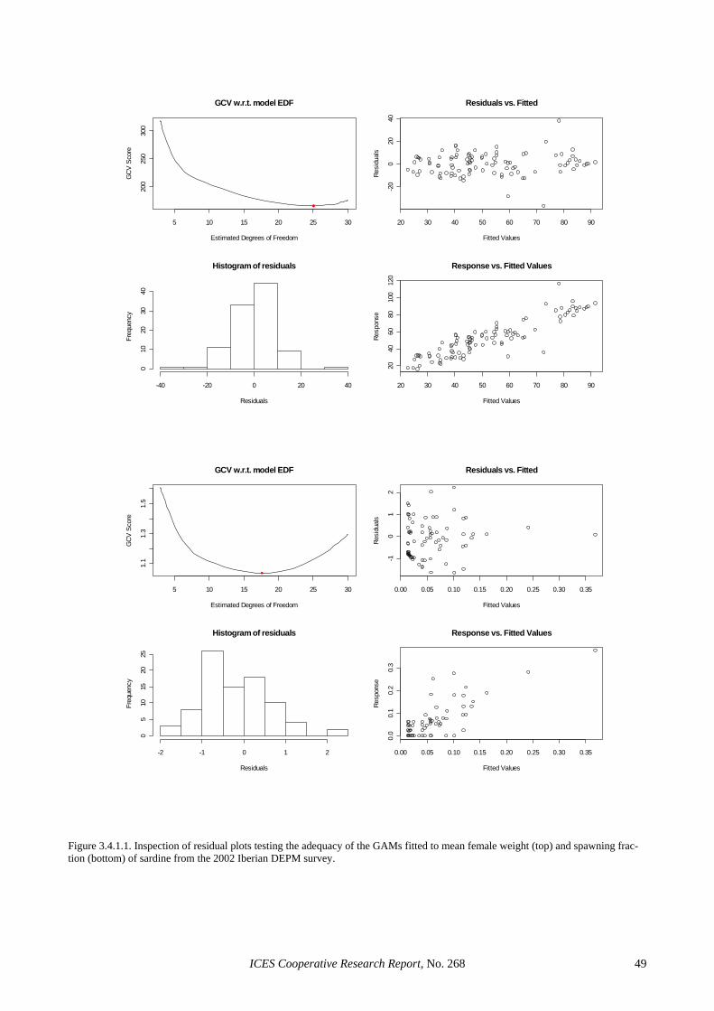
5 10 15 20 25 30
200
250
300
GCV w.r.t. model EDF
Estimated Degrees of Freedom
GCV
Sco
re
20 30 40 50 60 70 80 90
-20
020
40
Residuals vs. Fitted
Fitted Values
Resi
dual
s
Histogram of residuals
Residuals
Freq
uenc
y
-40 -20 0 20 40
010
2030
40
20 30 40 50 60 70 80 9020
4060
8010
012
0
Response vs. Fitted Values
Fitted Values
Resp
onse
5 10 15 20 25 30
1.1
1.3
1.5
GCV w.r.t. model EDF
Estimated Degrees of Freedom
GCV
Sco
re
0.00 0.05 0.10 0.15 0.20 0.25 0.30 0.35
-10
12
Residuals vs. Fitted
Fitted Values
Resi
dual
s
Histogram of residuals
Residuals
Freq
uenc
y
-2 -1 0 1 2
05
1015
2025
0.00 0.05 0.10 0.15 0.20 0.25 0.30 0.35
0.0
0.1
0.2
0.3
Response vs. Fitted Values
Fitted Values
Resp
onse
Figure 3.4.1.1. Inspection of residual plots testing the adequacy of the GAMs fitted to mean female weight (top) and spawning frac-tion (bottom) of sardine from the 2002 Iberian DEPM survey.
ICES Cooperative Research Report, No. 268 49
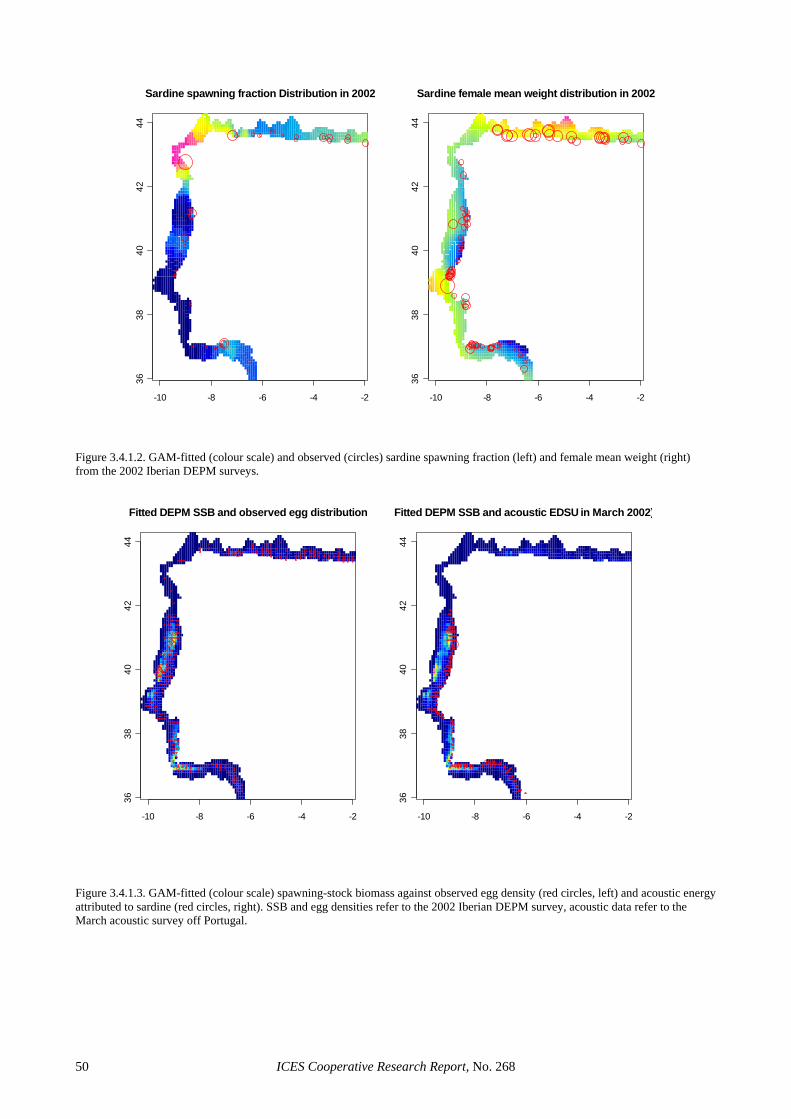
-10 -8 -6 -4 -2
3638
4042
44
Sardine spawning fraction Distribution in 2002
-10 -8 -6 -4 -2
3638
4042
44
Sardine female mean weight distribution in 2002
Figure 3.4.1.2. GAM-fitted (colour scale) and observed (circles) sardine spawning fraction (left) and female mean weight (right) from the 2002 Iberian DEPM surveys.
-10 -8 -6 -4 -2
3638
4042
44
Fitted DEPM SSB and observed egg distribution
-10 -8 -6 -4 -2
3638
4042
44
Fitted DEPM SSB and acoustic EDSU in March 2002)
Figure 3.4.1.3. GAM-fitted (colour scale) spawning-stock biomass against observed egg density (red circles, left) and acoustic energy attributed to sardine (red circles, right). SSB and egg densities refer to the 2002 Iberian DEPM survey, acoustic data refer to the March acoustic survey off Portugal.
ICES Cooperative Research Report, No. 268 50
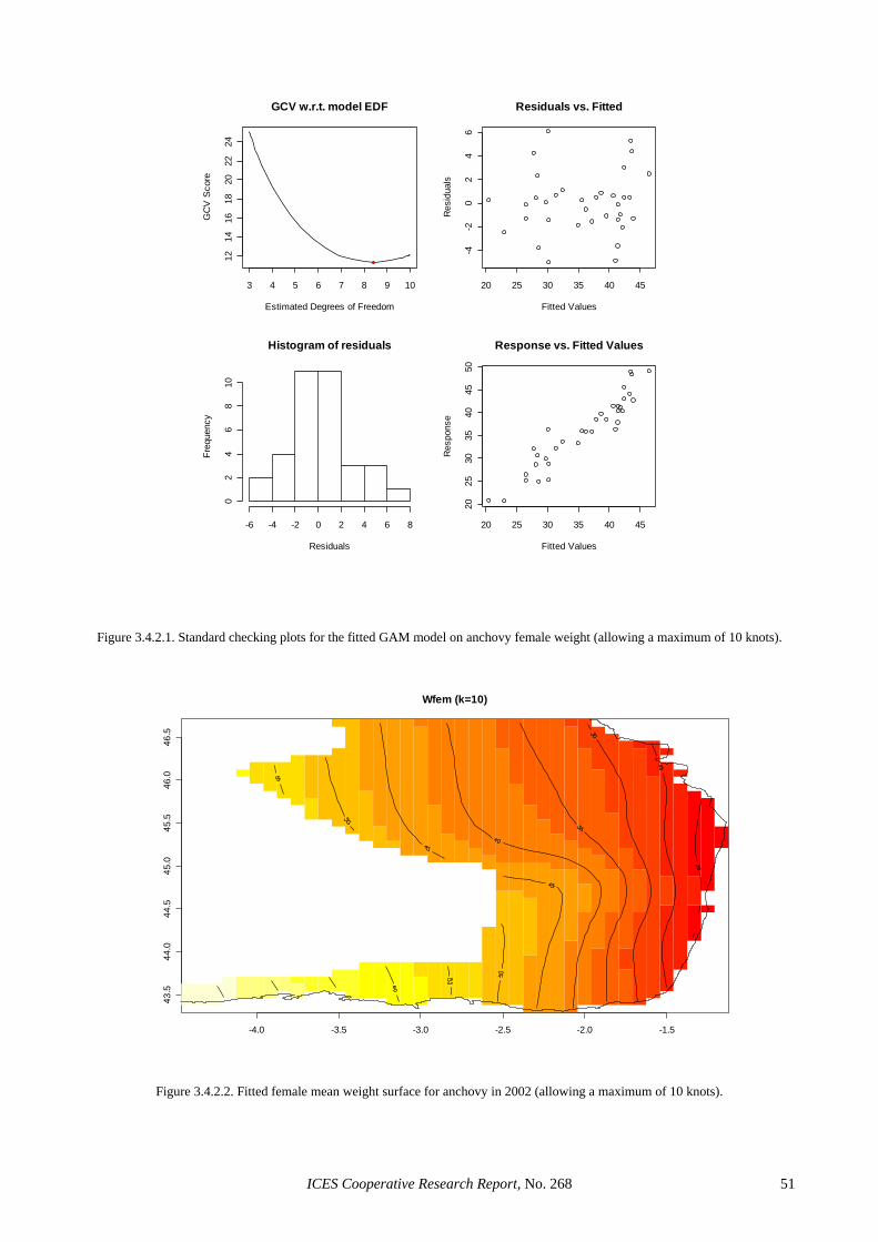
3 4 5 6 7 8 9 10
1214
1618
2022
24
GCV w.r.t. model EDF
Estimated Degrees of Freedom
GC
V S
core
20 25 30 35 40 45
-4-2
02
46
Residuals vs. Fitted
Fitted Values
Res
idua
ls
Histogram of residuals
Residuals
Freq
uenc
y
-6 -4 -2 0 2 4 6 8
02
46
810
20 25 30 35 40 45
2025
3035
4045
50
Response vs. Fitted Values
Fitted Values
Res
pons
e
Figure 3.4.2.1. Standard checking plots for the fitted GAM model on anchovy female weight (allowing a maximum of 10 knots).
-4.0 -3.5 -3.0 -2.5 -2.0 -1.5
43.5
44.0
44.5
45.0
45.5
46.0
46.5
Wfem (k=10)
Figure 3.4.2.2. Fitted female mean weight surface for anchovy in 2002 (allowing a maximum of 10 knots).
ICES Cooperative Research Report, No. 268 51
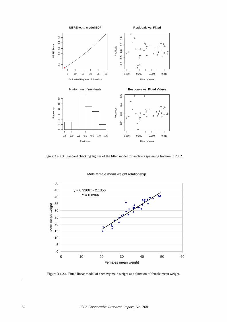
5 10 15 20 25 30
-0.4
0.0
0.2
0.4
0.6
UBRE w.r.t. model EDF
Estimated Degrees of Freedom
UB
RE
Sco
re
0.280 0.290 0.300 0.310
-1.0
-0.5
0.0
0.5
1.0
Residuals vs. Fitted
Fitted Values
Res
idua
ls
Histogram of residuals
Residuals
Freq
uenc
y
-1.5 -1.0 -0.5 0.0 0.5 1.0 1.5
02
46
810
12
0.280 0.290 0.300 0.310
0.2
0.3
0.4
0.5
Response vs. Fitted Values
Fitted Values
Res
pons
e
Figure 3.4.2.3. Standard checking figures of the fitted model for anchovy spawning fraction in 2002.
Male female mean weight relationship
y = 0.9208x - 2.1356R2 = 0.8966
0
5
10
15
20
25
30
35
40
45
50
0 10 20 30 40 50Females mean weight
Mal
e m
ean
wei
ght
60
Figure 3.4.2.4. Fitted linear model of anchovy male weight as a function of female mean weight.
.
ICES Cooperative Research Report, No. 268 52
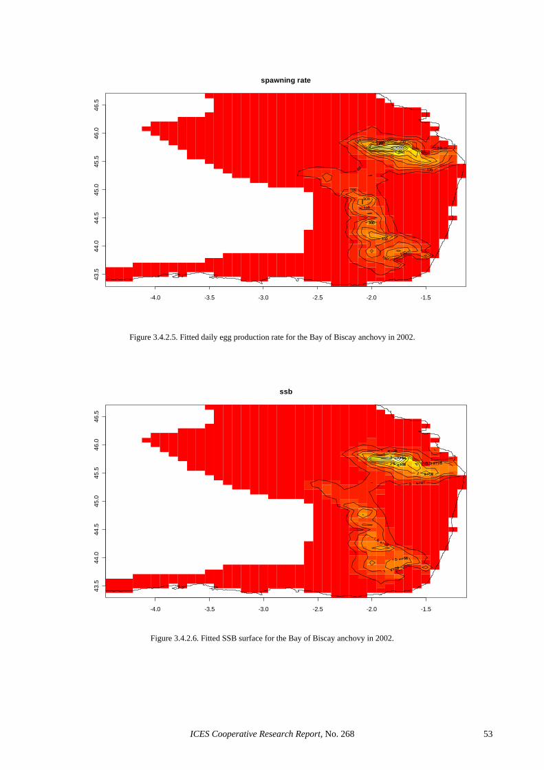
-4.0 -3.5 -3.0 -2.5 -2.0 -1.5
43.5
44.0
44.5
45.0
45.5
46.0
46.5
spawning rate
Figure 3.4.2.5. Fitted daily egg production rate for the Bay of Biscay anchovy in 2002.
-4.0 -3.5 -3.0 -2.5 -2.0 -1.5
43.5
44.0
44.5
45.0
45.5
46.0
46.5
ssb
Figure 3.4.2.6. Fitted SSB surface for the Bay of Biscay anchovy in 2002.
ICES Cooperative Research Report, No. 268 53
4 Other advances in DEPM methodology
This section includes research topics related to DEPM that have advanced in recent years, but for which the de-velopments have not been that far-reaching to warrant entire chapters. Section 4.1 is dedicated to the Continu-ous Underway Fish Egg Sampler (CUFES), providing a summary of recent advances, its application in DEPM surveys and its potential for the future. Section 4.2 is dedicated to egg staging and aging, where considerable progress has been made in the planning and execution of incubation experiments and the development of statisti-cally robust methods for modelling such data (see Sec-tion 3.2.1) and using them in the ageing of staged eggs. Section 4.3 is specific to the application of DEPM to Ibe-rian sardine, revising data on the maturation cycle of the species, comparing macroscopic and microscopic matur-ity scales and describing the seasonality of sardine spawning off Portugal. Finally, Section 4.4 is dedicated to spawning fraction estimation and the dating of post-ovulatory follicles, based on new data from sardine spawning populations in the north-eastern Atlantic (Ibe-rian Peninsula) and the eastern Mediterranean (Aegean and Ionian Seas).
4.1 The Continuous Underway Fish Egg Sampler (CUFES)
4.1.1 Introduction The Continuous Underway Fish Egg Sampler (CUFES) was developed in the 1990s (Checkley et al., 1997) and has proven efficient in sampling the highly contagious distribution of pelagic fish eggs and simultaneously col-lecting a wealth of oceanographic and spatial informa-tion. The sampler (which consists of a submersible pump, concentrator, electronics and sample collector) operates continuously at nearly all sea conditions, pro-viding a real-time estimate of the volumetric abundance of pelagic fish eggs at pump depth (usually 3 m). Apart from its obvious application in the characterization of spawning habitats (Van der Lingen et al., 1998; Check-ley et al., 1999a; Checkley et al., 1999b), it has also been used to improve the cost/precision ratio in the estimation of egg production in DEPM surveys (Lo et al., 2001; ICES, 2002). On the other hand, CUFES has some dis-advantages as an egg sampler than need to be taken into account: many eggs are damaged during the collecting process (which may bias estimates of daily production because younger eggs may be more vulnerable than older eggs), all egg stages may not be fully vulnerable to the pump (due to differences in the vertical distribution), se-lectivity problems may occur (particularly when 500 µm mesh size is used) and the samples may not independent leading to complicated variance formulations. Overall, accumulating evidence seems to indicate that CUFES performance as a quantitative sampler can be species-specific (depending on egg size, spawning depth and as-cending velocity rates) and habitat-specific (local envi-ronmental conditions that affect mixing/stratification
along the water column), precluding for the time being a global evaluation of its performance. For CUFES to be used in a DEPM survey, a way must be found to take ad-vantage of the high spatial resolution and rapid monitor-ing of characteristics of the instrument without giving up either precision or incorporating new biases.
Three possible ways for incorporating CUFES into a DEPM survey have so far been considered (ICES, 2002): i) Building a CUFES to CalVET conversion coeffi-
cient into the survey design, and use CUFES as the primary sampler, with CalVET only being used to convert the CUFES egg density to a full water col-umn value. Direct conversion of CUFES to a full water column tow would be expected to be impre-cise since the conversion factor would be a function of the specific gravity of the egg stage and the ex-tent of vertical mixing which may be highly variable within and between surveys. Computation of such conversion coefficients, largely support this view with R2 as low as 50% in some cases. Thus using the direct conversion method is likely to diminish any gains in precision that a CUFES-based DEPM might afford.
ii) Develop a mixing model with environmental co-variates to convert CUFES counts to full water counts, and use CUFES as the basic egg sampler while monitoring the environmental parameter that input the mixing model; a minimal CalVET sam-pling for validation purposes would only take place. In theory, if the extent of mixing and specific grav-ity of the eggs were known, one may be able to convert the abundance of eggs taken in CUFES to a full water column tow with reasonable precision and low bias. If this were possible, one would be able to carry out an entire DEPM egg survey without stop-ping the vessel, although a minimal CalVET sam-pling would always be desirable for ad-hoc valida-tion purposes. No such model has been developed and tested within the context of the DEPM, al-though general egg mixing models exist. Thus this option is in the realm of research direction, but it can not be already adopted with existing knowledge. Within EU project PELASSES work has been car-ried out in this direction (see following section) but additional results are needed before further evalua-tion of this issue can be made.
iii) Use CalVET as the primary sampler and use CUFES to map the spawning area and to schedule the sampling of CalVET samples. Improvement in the design of CalVET-based plankton surveys can be obtained with CUFES. For example, in the Bay of Biscay anchovy DEPM surveys presence and ab-sence of eggs in CUFES at the outer edges of the expected spawning distribution is being used to de-cide whether to abandon or not the coverage of ra-dial tracks, while the CUFES abundance serves to identify areas where sampling could be intensified. A more thorough implementation of CUFES in the design and estimation of CalVET-based DEPM sur-veys for sardine is found in California (Lo et al., 2001). A rule is established to start CalVET sam-
ICES Cooperative Research Report, No. 268 54
pling along a radial transect conditioned on egg densities in CUFES being above a threshold of 2 eggs per minute. This leads to a spatial stratification of the sample according to abundance, those of low abundance being only covered by CUFES whereas in areas of high egg abundance both CUFES and CalVET are hauled. Daily egg production is primar-ily calculated for the later area and the total area es-timation is based on a raising factor according to the CUFES egg density ratio in the two strata.
Section 4.1.2 describes recent advances in the compari-son of CUFES with vertical plankton samplers, Section 4.1.3 summarizes the use of CUFES in the most recent sardine DEPM survey, while Section 4.1.4 highlights other potential uses for this sampler. Finally, Section 4.1.5 synthesizes the opinion of SGSBSA on the poten-tial use of CUFES in the DEPM for the near future.
4.1.2 Summary of results from PELASSES The spring acoustic surveys of Portugal, Spain and France were internationally coordinated during 2000 and 2001 (PELASSES project), covering the area from the Gulf of Cadiz to the northern Bay of Biscay and follow-ing a standard survey design and sampling methodology. As part of this methodology, CUFES was for the first time used simultaneously with acoustics to map the dis-tribution of pelagic fish eggs and thus offer auxiliary in-formation for acoustic estimation. In addition, CUFES was tested for the first time as a quantitative sampler for the estimation of sardine and anchovy egg abundance in the water column. For that, apart from the direct com-parisons between with CalVET/PAIROVET (Section 4.1.2.1), the vertical distribution of eggs was described in the inner Bay of Biscay and a model for the estimation of egg abundance in the water column based on CUFES and oceanographic data was developed and tested (Section 4.1.2.2).
4.1.2.1 CUFES and CalVET/PAIROVET experi-mental sampling
Stratoudakis et al. (2001) presented preliminary results from the comparison between CUFES and CalVET egg samples simultaneously collected during the spring 2000 PELASSES survey off Portugal and the Gulf of Cadiz. Data from vertical plankton tows (CalVET), simultane-ous CUFES samples of 4 minutes duration and underway CUFES samples of 1.5 nm fixed length (immediately be-fore and after each fixed station) were collected in 118 locations along the continental shelf of the survey area. Among the 4 sets of samples, stationary CUFES indi-cated sardine and anchovy egg absence more frequently than CalVET and underway CUFES (the latter generally outperforming CalVET in egg detection), although sar-dine egg presence/absence agreement among all sets of samples was relatively high (73–81%). Sardine egg den-sity estimates in the 4 sets of samples were generally cor-related (log-scale), with a relatively small group of outly-ing stations showing persistent differences between CalVET and the 3 CUFES samples (before, during and after CalVET). The latter indicated that such pronounced differences in the performance of the two samplers are
probably related to uncharacteristic vertical egg distribu-tions, themselves resulting from local water column mix-ing conditions.
Additional work on the comparison of the two sam-plers, as well as on the comparison of CUFES perform-ance between vessels and years, was performed during the PELASSES surveys in the Bay of Biscay (AZTI and IFREMER). Uriarte et al. (2003) present a broad com-parison of PAIROVET (two CalVET nets, Smith et al., 1985) and CUFES, based on the analysis of two years of coupled surveys performed in the Bay of Biscay almost simultaneously by RV “Investigador” (rented by AZTI) and RV “Thalassa” (IFREMER). In spring 2000 and 2001, the two vessels performed experimental paired sampling of PAIROVET and CUFES for anchovy and sardine eggs. Paired sampling was performed over a wide area within the Bay of Biscay, aiming to cover a wide range of environmental and oceanographic condi-tions. The results showed that CUFES is a powerful sampler for egg detection (equal or superior to PAIROVET), particularly for sardine eggs (see also Sec-tion 4.1.3). While the probability of detecting sardine eggs in underway CUFES but not in PAIROVET ranged between 44–55%, the probability of detecting sardine eggs with PAIROVET but not with CUFES ranged be-tween 11–22% (Uriarte et al., 2003). This implies a higher power of sardine egg detection for CUFES than for PAIROVET. Van der Linger et al. (1998) also found higher probability of detecting sardine (Sardinops sagax) eggs with CUFES than with PAIROVET, but they found the contrary for anchovy (Engraulis capensis). Recent evidence (M. Santos, pers. comm.) suggests that selectiv-ity of anchovy eggs by the CUFES may be responsible for this discrepancy, given that anchovy eggs were often found to pass through the mesh and lost from the sample held in the collector.
However, CUFES provided a poor representation of egg abundance in the water column during the PELASSES surveys in the Bay of Biscay, with CVs ranging from 75%–100%. The relationship between PAIROVET and CUFES is affected by the vessel itself (probably due to the type of hull) and changes between years. In addition, in RV “Investigador” this relationship changed with the motion of the vessel (stationary or un-derway), probably linked to the turbulence and mixing induced by the vessel while moving. RV “Investigador” showed an increase of about 50% for anchovy and 25% for sardine in the efficiency of egg catching with CUFES on station in comparison to underway sampling (Figure 4.1.2.1.1). This is consistent with previous observations made on the same vessel for anchovy (Bez, 2000). This effect was also noted by Van del Linger et al. (1998) for round herring (Etrumeus whiteheadi), but was not de-tected for sardine. The analysis showed statistically sig-nificant year and vessel effects for both species (with the exception for anchovy, where non significant differences were found between vessels in 2000, Table 4.1.2.1.1). This is a discouraging result concerning the goal of stan-dardising the CUFES sampling performance among years or vessels.
Stratoudakis et al. (2001) and Uriarte et al. (2003) showed that the fraction of eggs which are partly dam-aged is far higher in CUFES than in CalVET/-
ICES Cooperative Research Report, No. 268 55
PAIROVET, in the latter study ranging between 38–57% for anchovy and between 15–21% for sardine. This is probably caused by the increased mechanical pressure exerted on eggs during pumping and concentration. For damaged eggs, only some broad stage grouping is gener-ally possible, such as NE (no embryo), EE (early em-bryo) and LE (late embryo). In addition, the percentage of damaged eggs depends on egg stage, with the young-est eggs (NE) being considerably more vulnerable than LE ones. For these reasons, any use of egg stages ob-tained with CUFES should mostly be based on broad staging groups (see Section 4.1.3).
4.1.2.2 CUFES as a quantitative sampler of egg abundance in the water column
The poor precision of CUFES as an estimator of egg abundance in the water column can be partly reduced by modelling the vertical egg distribution (with or without the incorporation of environmental covariates). Specific experimental sampling was carried out by MBA and AZTI with the Longhurst-Hardy Plankton Recorder (LHPR, Williams et al., 1983) along with CUFES and PAIROVET sampling. LHPR was used to describe the vertical distribution of anchovy and sardine eggs accord-ing to the physical structure of the water column and wind forcing. In addition, the Density Gradient Column (Coombs et al., 1985) was used to measure egg buoy-ancy. Stratified vertical sampling was used to tune a model of vertical distribution of epipelagic eggs that use buoyancy, physical conditions of the water column (in-cluding turbulence), and spawning depth (Sundby, 1991). The purpose of this study (Boyra et al., 2003) was to model and predict the depth distribution of sardine and anchovy eggs under different oceanographic conditions and to quantify the proportion of eggs sampled by CUFES at 3m depth. Sundby’s (1983) model for the ver-tical egg distribution was improved through modifica-tions of the vertical propagation of wind-induced turbu-lence. Measurements of egg settling velocity and buoy-ancy by stages were incorporated, including adaptability of the latter to the environment. The model was generally successful in describing the dependence of the vertical egg distributions on the density profiles of the water col-umn and wind induced turbulence at surface. The coeffi-cient of determination was rather similar for sardine and anchovy vertical egg distributions: around 80% (geomet-ric mean of R2 at all environmental scenarios), indicating a significant improvement over previous models. How-ever, while in high surface salinity environments R2 of almost 90% were achieved, these were reduced to about 70% in the low surface salinity cases, suggesting that ad-ditional research is required in the latter. Boyra et al. (2003) also compared the modelled vertical egg distribu-tions to those observed during the PELASSES surveys, by considering the goodness of fit of the model predic-tion to the egg density at 3 m depth (LHPR samples), av-eraged within the main environmental scenarios (Figure 4.1.2.2.1 and 4.1.2.2.2). For low salinity stations, relative errors of about 30% were common for both species, with no indication of systematic pattern in the deviations. In high salinity areas the errors were smaller, particularly for sardine. However, in individual LHPR stations the re-
lationships were rather noisy and the same was observed in preliminary analysis of the CUFES egg densities in these stations (Boyra, pers. comm.). Individual fitting was worse than that achieved for the average by envi-ronmental scenarios and hence the potential application of the model of vertical distribution cannot be, yet, prop-erly assessed. Additional research is currently underway aiming to provide more conclusive results on the appli-cability of CUFES as a quantitative sampler of egg abundance in the water column (Uriarte, pers. comm.).
4.1.3 The use of CUFES in the 2002 sardine DEPM survey
In the 2002 DEPM surveys for the Atlanto-Iberian stock of sardine, CUFES was used for the first time to delimit the spawning grounds and to allocate CalVET sampling effort (see Section 2.4.1). Table 4.1.3.1 presents the re-sults of the comparison between the performance of CalVET and CUFES in the Portuguese survey. Compari-sons were based on presence/absence of eggs in the CUFES sample obtained along the 3 nm leading to a CalVET station and the respective CalVET sample. In the 470 samples considered, the percent of discordance was 24%, with 6% indicating only CalVET presence and 18% indicating only CUFES presence of sardine eggs. The higher probability of egg detection by CUFES is probably due to the larger area covered and amount of water filtered by CUFES, confirming that it consists a powerful sampler to delimit sardine spawning grounds. Figure 4.1.3.1 shows that similar results are obtained when the presence of sardine eggs in CalVET and CUFES is separately compared for broad groups of egg stages (loosely termed Day-1, Day-2 and Day-3 groups). In the Spanish survey, a calibration was carried out in the Bay of Biscay along 7 transects perpendicular to the coast, where both samplers were used simultaneously. A total of 54 samples were obtained with CalVET and 54 x 3 with CUFES (following the sampling design used in PELASSES). Comparison of performance of CUFES at, before and after the CalVET stations (Table 4.1.3.2) show a high degree of within-CUFES consistency, with agreement ranging from 85 – 96%. Comparison between CalVET and CUFES (Table 4.1.3.3) also shows good agreement between samplers, although unlike other ob-servations (Stratoudakis et al., 2001; Uriarte et al., 2003; and the Portuguese 2002 survey), CUFES did not per-form CalVET in the detection of sardine eggs. To verify differences between the proportion of different develop-ment stages obtained from CUFES and CALVET, the positive stations were analyzed (37 CalVET and 105 CUFES). Samples from CUFES were classified using two staging scales; one considering the four classes de-scribed in Section 4.1.2.1 (no embryo, early embryo, late embryo and disintegrated) and another using the standard 11 stages described by Gamulin and Hure (1955), see also Annex 1. Eggs from CalVET were classified only into 11 stages, but for comparison purposes were also grouped in the broader four classes. Overall, there were no large differences between the stage distribution ob-tained by CUFES and CalVET, although it is again evi-dent that CUFES damages eggs more often than CalVET (Figures 4.1.3.2 and 4.1.3.3).
ICES Cooperative Research Report, No. 268 56
4.1.4 Using CUFES to test DEPM assumptions Traditional DEPM estimation of egg production is based on the assumption that daily production is constant over time and along the survey area. GAMs can relax the as-sumption of spatial stationarity, but still assume that on any given location production is constant over time and all cohorts present in the water column are adequately sampled by the vertical plankton tows. However, these assumptions can be violated by egg transport (it is known that egg distribution is affected by advection and diffu-sion) and/or spatio-temporal variation in reproduction (very little is known on the fine scale dynamics and be-haviour of reproductive schools of small pelagic fish).
CUFES (coupled with acoustics) provides a unique means of obtaining synoptic views of the fine-scale egg and fish distribution at a narrow fine spatio-temporal scale, thus allowing testing of the above assumptions. A first application with this objective was performed during the November 2001 Portuguese acoustic survey (Zwolinski, 2003). Two small areas in the Gulf of Cádiz and in the Algarve (approximately 120 nm2 each), were sampled intensively for one night with CUFES. Eleven parallel transects 1 nautical mile (nm) apart and 10 miles long were performed in each zone. Individual CUFES samples were taken at 6 minutes intervals of underway sampling, in order to obtain samples from approximately 1nm. Based on these data, Zwolinski (2003) described the autocorrelation structure within daily egg patches (evidence of diffusion) and the small-scale differences in the distribution of sequential daily egg patches (Figure 4.1.4.1). The latter is useful in showing that small-scale spatial variation (either due to small shifts in the location of spawning schools or due to egg displacement after re-lease) can increase considerably the noise/signal ratio of CalVET samples (which are meant to provide estimates for all daily cohorts locally released in the 2–4 days up to sampling). For example, under a standard DEPM survey the area depicted in Figure 4.1.4.1 would probably be covered by 6–9 CalVET stations, where (depending on the location) eggs from either or both cohorts would have been detected in widely varying relative abundances.
4.1.5 Recommended use of CUFES in future DEPM surveys
The main aim of most of the research presented above is to evaluate the potential of CUFES to substitute CalVET/PAIROVET as the primary quantitative egg sampler in future sardine and anchovy DEPM surveys. The results so far indicate that, although CUFES is a powerful sampler for egg detection (equal or superior to CalVET/PAIROVET), there are still important problems to resolve before it can be considered as a quantitative estimator of sardine and anchovy egg abundance in the water column. Precision in the estimation of egg abun-dance in the water column by CUFES is poor, while sig-nificant effects due to motion, vessel and year provide additional complications. Poor precision can only be partly remedied by modelling the vertical egg distribu-tion that incorporates environmental covariates into the model formulation. However, sufficiently accurate and precise model predictions of aerial egg abundance are still not available for all oceanographic conditions en-
countered in stratified environments, and further work is undergoing. In addition, CUFES shows a marked selec-tivity of anchovy eggs (ICES, 2003b), but this is less clear for sardine eggs. Based on the above, the group recommends that CUFES continues to be used in the next DEPM surveys for anchovy and sardine as an auxil-iary sampler (along the lines defined in ICES, 2002), but this recommendation can be revised when additional re-sults become available.
4.2 Egg staging and ageing This section reports on significant recent advances in the staging and ageing of sardine and anchovy eggs for DEPM purposes. Section 4.2.1 summarizes the results of a recent staging workshop that took place before the 2002 surveys, as a result of a recommendation from the previous group meeting (ICES, 2002). Section 4.2.2 de-scribe the application of new methods of analysis to old and new egg incubation data for sardine and anchovy, while Section 4.2.3 identifies factors other than tempera-ture that may also affect pelagic egg development. Fi-nally, Section 4.2.4 reviews existing information on the daily spawning activity of sardine and anchovy, high-lighting its importance in egg ageing.
4.2.1 Staging workshop During the first meeting of SGSBSA (Lisbon, October 2001), an informal workshop was performed to obtain reference collections of sardine and anchovy egg stages (see Annexes 1 and 2) and to assess the consistency in egg staging among institutes and readers. Significant dif-ferences were reported among institutes, particularly in relation to the criteria used to classify eggs as destroyed (ICES, 2002). As a result, a workshop was proposed to take place within the framework of PELASSES, before the analysis of the 2002 DEPM samples.
The meeting took place in San Sebastian during January 2002. The main objective of the workshop was to identify the main differences between readers and in-stitutes and to unify staging criteria. A first staging of anchovy and sardine eggs obtained with PAIROVET and CUFES samplers was carried out to identify the differ-ences between individuals and groups (scientists from IFREMER, AZTI, IEO and IPIMAR). Anchovy and sar-dine eggs were staged in 11 stages (Moser and Ahlstrom, 1985; Gamulin and Hure, 1955) for the eggs collected with PAIROVET and in 3 stages for the eggs collected with CUFES. Those 3 stages were No Embryo (NE), Early Embryo (EE) and Late Embryo (LE) that is a grouping of the eleven stages (definition proposed by PELASSES and adopted by this Study Group). Stage NE grouped stages I, II and III, stage EE grouped stages IV, V, VI, and stage LE grouped stages VII to XI.
During the first staging, each participant used the cri-teria that were normally employed for routine staging. The percentage of agreement was measured with respect to the modal stage weighted by the reader experience (Eltink et al., 2000). After the analysis of the data from the first staging, the identification criteria for each stage were discussed and the group complemented the defini-tions of each development stage for anchovy and sardine
ICES Cooperative Research Report, No. 268 57
based on the original ones of Moser and Ahlstrom (1985) and Gamulin and Hure (1955). A second staging subse-quently took place, using the revised definitions for each stage. The analysis of the second set of data demon-strated that the percentage of agreement increased for both species (Tables 4.2.1.1 to 4.2.1.3). The improve-ment was bigger for anchovy (15% for PAIROVET and 10% for CUFES), probably due to the relatively limited previous experience in the staging of anchovy eggs at some institutes. For sardine improvements were also reg-istered (8% for both PAIROVET and CUFES) and this was subsequently reflected in the reduction of discrepan-cies in the percentage of destroyed eggs in the Portu-guese and Spanish 2002 surveys (Table 4.2.1.4).
4.2.2 Analysis of new and published egg incubation data for sardine and anchovy
Two methods were used to analyse the evolution of egg stages through ages for different temperatures, using data from published and new incubation experiments. The new ageing method (developed within the GAMs project and described in Section 3.2.1) and the traditionally used ageing method (Lo 1985) were both applied to analyze data from the anchovy and sardine incubation experi-ments.
The traditional ageing method is based on fitting the incubation experiment data by the model proposed by Lo (1985):
321 0,θθθθ iea it
ti+= (1)
where t denotes temperature, i stage, tia , mean age
within stage i incubated at temperature t and 0θ , 1θ , 2θ
and 3θ are the model parameters. Estimates of tia , were computed for sardine and anchovy as the mean elapsed time from the beginning of an incubation experiment up to the checking time, weighted by the number of obser-vations of each development stage (Miranda et al., 1990; Motos, 1994). Then, model (1) was fitted to the incuba-tion data usually by least squares on the log-transformed equation. The ageing method described in Section 3.2.1 is based on the fitting of a multinomial model to the in-cubation data. In contrast to Lo’s model, this approach considers age and temperature as fixed explanatory vari-ables and stage as a random variable. For each stage i the conditional probability of an egg being at stage i or above given that the egg is in stage i-1 or above is mod-elled by fitting a binomial generalized linear model (GLM) depending on age and temperature. The probabil-ity of an egg being in each stage can therefore be derived as a product of the fitted conditional probabilities. The multinomial model was fitted using the package dep-model (Section 3.2.5).
In the case of anchovy (Section 4.2.2.1), the new method was applied to existing incubation data (Motos, 1994), while in the case of sardine both existing (Miranda et al., 1990) and new incubation data (experi-ment carried out in 2002 by IEO) were used in the analy-sis (Section 4.2.2.2).
4.2.2.1 Anchovy The incubation experiment for anchovy (Motos, 1994) was carried out in May-June 1992 during the annual DEPM survey on board RV “Cornide de Saavedra”. Two incubations, in two distinct locations, were performed us-ing five completely hydrated females and five mature males selected from the tow. After inciting the females to spawn by an abdominal massage, the eggs were mixed with sperm and kept in a tube. When the first cellular di-visions were detected, the eggs were placed in 50 ml glass tubes in an incubator block. Two rows of seven tubes were prepared and positioned across the block cov-ering a temperature range from 8º to 22ºC (Table 4.2.2.1.1) Eggs were randomly sampled at regular inter-vals from each tube. For each sample the elapsed time from the beginning of the experiment, the temperature and the number of eggs in each developmental stage (Moser and Ahlstrom, 1985) were recorded. Given the difficulty of distinguishing stage I eggs from non-fertilized ones, stage I eggs were excluded from the stage classification. At each sampling period, dead eggs were removed from the tubes and seawater from a reserve held at the same temperature was added to maintain a similar water level in the tube during the whole experiment. Sampling from each tube finished when eggs had begun hatching or when there were no more eggs to sample (all the eggs were already sampled or dead).
Given that the temperature gradient was stable and similar in both incubations (Table 4.2.2.1.1), and assum-ing that there was no difference between incubations, data were gathered and analysed jointly. The observed (age, stage) data are shown in Figure 4.2.2.1.1. Expected values from Lo’s model for the observed temperatures and for all stages are shown in Figure 4.2.2.1.2. Two models were considered. The first assumes that the ef-fects of the explanatory variables, age and temperature, were the same across stages, while the second allows for the coefficients of age and temperature to differ among stages. The first model was found to be inadequate for these incubation experiment data. The second, more flexible model, provided a substantially better fit to the data and was selected for assigning ages to anchovy eggs (Figure 4.2.2.1.3).
In general, multinomial models allow a better and more natural way of analysing incubation experiment data (the development of each stage egg is not determi-nistic), while introducing additional flexibility (variabil-ity is better reflected by means of a multinomial model). Furthermore, hatching time can be derived directly from the multinomial model, instead of fitting a second model to the age-assigned eggs. There are alternative models available in R (www.r-project.org) for fitting the multi-nomial distribution of ordered categorical random vari-ables as stages, with probabilities depending on explana-tory variables like age and temperature. For example, proportional odds models (that model cumulative prob-abilities and assume that the effect of the explanatory variables are identical for all categories) can be fitted us-ing the function polr in the library Mass. The function lrm from the libraries Hmisc and Design allows also fit-ting the conditional probability of being in one category given that it is in the previous category or above using
ICES Cooperative Research Report, No. 268 58
the logit link (the so-called continuation-ratio models). These approaches were also investigated as part of the GAMs project, where the model adopted in depmodel and used here was found to outperform all others for the incubation data at hand.
4.2.2.2 Sardine A new incubation experiment for sardine was success-fully carried out by IEO in 2002, following the recom-mendation of the previous Study Group meeting (ICES, 2002). The incubation experiment was performed ac-cording to that described for anchovy (Motos, 1994 and Section 4.2.2.1), using the same incubator. Eggs were obtained from a survey onboard RV “Vizconde de Eza” in the Gulf of Cádiz (SW Spain) between 10–17 Febru-ary 2002. Sardine adults were caught using a commercial trawl, and eggs and sperm were extracted from macro-scopically identified spawning sardines. Hydrated eggs were obtained by abdominal pressure and immediately fertilised by sperm collected from males. Once fertilised, viable eggs were placed in small jars filled with filtered seawater within the incubator. Five temperatures within the range of 11 to 17oC were used in the experiment (Ta-ble 4.2.2.2.1). Five replicates for each temperature and around 200 eggs for each replicate were used in the ex-periment. Two additional jars with filtered water were placed in each row corresponding to each temperature used in the analysis, in order to allow for refilling of the egg jars with water at the same temperature.
Samples from each temperature of the incubator were taken randomly from one of the replicates of that tem-perature in each sampling event. On the 6 first hours of the experiment samples were taken at 1 hour intervals, and, afterwards, the sampling frequency was set to 3 hours up to hatching. Around 30 eggs for each tempera-ture were sampled each time (Table 4.2.2.2.1), and for each sample, elapsed time from the starting of the ex-periment, temperature, replicate number and stage of each of the sampled eggs were recorded. After being staged (Gamulin and Hure, 1955), eggs were returned to the same jar, and any loss of water was replaced. Addi-tionally, at least twice a day, all dead eggs were siphoned from the bottom of the jar and the water volume was re-filled from filtered water at the same temperature. With this procedure, at least 1/3 of the water volume was re-newed each day.
The observed (age, stage) data are shown in Figure 4.2.2.2.1. Figure 4.2.2.2.2 shows both the published model from Miranda et al. (1990) and the Lo model fit-ted to the Cádiz incubation experiment (with stage dura-tion estimated using observed standard deviation on stage age). The multinomial model of the evolution of stages through ages for different temperatures is shown in Figure 4.2.2.2.3, together with the observed evolution of percentage of eggs in each stage for different observed times (ages) and temperatures.
The original data from Miranda et al. (1990) were not available to refit the models, and thus only the data from the Gulf of Cádiz were used to assign ages to sardine staged eggs using the new ageing methods. The multi-nomial model was found to perform better than the tradi-tional (Lo’s) model with the sardine incubation data. The
multinomial model has two main advantages over the traditional models when applied to these data. First, it has a sound theoretical basis (as explained in Section 3.2). Age (i.e., sampling time) is fixed in most incubation experiments and stage is the random variable observed, and this is the way the data are treated in the multinomial approach, but not the traditional one. Also, stage is a fac-tor (a discrete variable) and fitting a model like Lo’s that treats stage as continuous, has the difficulty of not know-ing a-priori the stage duration, i.e., the spacing on the x-axis. Second, the traditional way of treating incubation experiments is to fit a model to the mean age of the stages as a function of stage and temperature and then to fit a separate model to stage duration. Two models of stage duration as a function of stage and temperature have been used in the literature: • Constant stage duration for a given stage for any
temperature (Lo, 1985; Motos, 1994), or
• Continuous model of stage duration as a function of stage and temperature (Miranda et al., 1990).
As shown by the data (Figure 4.2.2.2.1), stage duration changes both with stage and temperature. Nevertheless, stage duration cannot be represented by a monotonous function of stage, as stages III and IV consistently show a shorter duration than other stages. The multinomial models pick the lower probability of stages III and IV adequately from the data, and provide a natural way to interpolate the probability of being at any stage for a given age and temperatures not observed on the incuba-tion experiment but within the observed range. There are different ways and available software packages to fit a multinomial model to data like the one obtained from an incubation experiment. In general the fitting procedure included within depmodel provides more flexibility to represent the transitions between the stages and models the data from the Cádiz experiment adequately. How-ever, one disadvantage of this extra flexibility is that it produces longer tails (non-zero probabilities of being in any given stage, at ages far greater than the mean age at that stage), increasing (maybe artificially) the range of possible ages for a given stage.
4.2.3 Factors other than temperature affecting egg development
Very few studies have so far described the effect of fac-tors other than temperature on egg development, al-though it is accepted that such factors exist and also af-fect the probability of survival. Stratoudakis et al. (1998) and Steer et al. (2002) have demonstrated the impact of factors other than temperature (vertical position within multi-layer mats, salinity) to the development and mor-tality rates in the demersal eggs of herring (Clupea harengus) and southern calamary (Sepioteuthis australis) respectively. In the case of pelagic fish eggs, egg size is known to affect mortality rates (Pépin, 1991), while also acting as an index of egg condition resulting from paren-tal investment. More recently, egg size in combination with salinity and oxygen concentration have been re-ported as crucial to the survival and development of cod eggs (Vallin and Nissling, 2000). Finally, several studies
ICES Cooperative Research Report, No. 268 59
on the biochemical composition of pelagic fish eggs and larvae in relation to environmental and parental effects have been recently carried out around the Iberian penin-sula (Riveiro et al., 2000, Guisande et al., 1998, Verea et al., 1997). Parental condition and age seem to affect egg size and biochemical composition in pelagic fish, al-though results need to become more conclusive.
To the best knowledge of this Study Group, no incu-bation experiments so far, have taken into account fac-tors other than temperature in the estimation of develop-ment rates. There is a potential scientific field for study-ing the relationship between egg development (and mor-tality) and environmental variables other than tempera-ture, as well as taking into account biotic variables like parental condition. Such studies may help to understand environmentally-driven recruitment variability, which is largely dependent on variability in egg, larval and post-larval survival. Further, accounting for variability in egg development due to factors other than temperature may also help to improve egg ageing for DEPM purposes. Due to the Bayesian nature of the ageing method pre-sented in Section 3.2.1, any new information on incuba-tion experiments that include other environmental and/or biological variables can be incorporated in the ageing procedure, with a potential improvement in ageing preci-sion.
4.2.4 Assumptions on daily spawning For the application of the DEPM to small pelagic fish species with daily spawning synchronicity, time of peak spawning must be known to age eggs according to their observed stages and sampling time (e.g., Lo, 1985; Bernal et al., 2001). This procedure is necessary to ob-tain egg densities and mean ages for each daily cohort in the sample and thus estimate daily egg production and mortality. In addition, the new Bayesian approach for as-signing ages to egg stages (see Section 3.2.1) requires a probability function of spawning time. Assuming a nor-mal distribution, this implies, in addition to the time of peak spawning, that the standard deviation of daily spawning activity from the peak is also known to identify uniquely the daily spawning probability density function (SPDF). In the remaining of this section, the information available for estimating these two parameters for an-chovy and sardine is revised and gaps in current knowl-edge are highlighted.
In the case of anchovy, Motos (1994) used observa-tions on the reproductive state of spawning females and on the prevalence of stage I eggs in the plankton (data from 1989 to 1992) to suggest that peak spawning occurs around midnight. This estimate of peak spawning time has been used in the traditional application of the DEPM to anchovy until now. However, data from another dec-ade are now available, allowing a revision of this infor-mation based on a considerably wider set of data than those originally available to Motos (1994). The repro-ductive state of adult females is reviewed using histo-logical data from the surveys of 1990–1992, 1994, 1995, 1997, 1998, 2001, and 2002. The incidence around mid-night of females that are to ready spawn or that have al-ready spawned in the night was analysed as in Motos (1994), in order to identify the exact time that those al-
ready spawned are more frequent in the sample those that are still to spawn in the same night. In addition, the inci-dence of stage I in the plankton around midnight was also analysed as indicative of the effective realisation of the spawning act by adults.
Figure 4.2.4.1 shows the evolution of the gonad state of spawning females in samples collected from 18:00 to 6:00 (data pooled across years). The transition of the predominance of pre-spawning (hydrated) females to post-spawning females (gonads with POFs) occurs be-tween 23 and 24 hours, while between 23.5 and 24 hours post-spawning females attain about half of the spawning females. Overall, the presence of spawning females (hy-drated and POFs) reach its maximum between 23 and 24 hours and particularly between 23.5 and 24 hours. The range of spawning times as revealed by spawning fe-males mainly extends from 21 to 1.5 hours (i.e., a spawn-ing range of 4.5 hours), being negligible the spawning occurring before or after. However, a minor, but persis-tent across years, secondary peak of spawning seems to occur between 4 – 5 in the morning.
Figure 4.2.4.2 shows the incidence of stage I eggs per surface unit during the 1994–2002 surveys, overlaid to the expected stage I distribution arising from the fitting of a normal distribution to the spawning time. This direct fitting suggests that a peak spawning time at 23.25 hours (23 hours and 15 minutes) with a 2 hours standard devia-tion would best explain the observed stage I egg distribu-tion if duration of that stage is 1.33 hours. However, con-sidering only the period 1996–2002, the optimum peak spawning time would be 23:00 hours with a SD of 1.7. It should be noted that both estimates are based on the re-strictive assumption that stage I eggs last 1.33 hours, but this is a minimal duration of that stage and therefore the indication from those eggs is that peak spawning is to be considered to take place at the latest at 23:15. Overall, revised adult and egg data seem to confirm that peak spawning for anchovy in the Bay of Biscay must be be-tween 23 and 24 GMT hours, with the best estimate of SPDF from these data being ~N(23, 1.25).
In the case of sardine, existing DEPM applications have assumed a 19:00 GMT peak in spawning activity (Cunha et al., 1992; García et al., 1992). However, the assumption was based on less exact data than in the case of anchovy, although there is little doubt that sardine also shows considerable daily synchronicity in spawning, most likely towards dusk (Ré et al., 1988; Bernal et al., 2001). Zwolinski et al. (2001) showed that the gona-dosomatic index and the density and diameter of hy-drated oocytes within the gonad follow a consistent daily pattern in female sardine that are expected to spawn on the same day (Figure 4.2.4.3). The same Figure also shows that until 18:00 hydrated females did not show any evidence that spawning had already started (i.e., no POFs were found during the histological inspection of the gonads). On the other hand, plotting the hourly dis-tribution of stage I eggs from all Iberian DEPM surveys (Figure 4.2.4.4) demonstrates a peak in egg density around 22:00 GMT. This matches well the observed daily distribution of sardine spawning in a fixed location repeatedly sampled within a day (Ré et al., 1988) and with more recent evidence from intensive adult sampling during the end of the day (Ganias et al., 2003b). Figure
ICES Cooperative Research Report, No. 268 60
4.2.4.2 also shows that a SPDF with 0.5h standard devia-tion seems to fit more adequately the data from a single location (Ré et al., 1988), while one with 1h sd seems more appropriate for data collected across DEPM sur-veys. Overall, this evidence seems to contradict the cur-rently assumed location of the SPDF for sardine, but more detailed information is needed for the group to rec-ommend an alteration to the assumed SPDF (which is currently set as N~(19,1)). This is because changes in the duration of daylight along the spawning season (the data of Ré et al. (1988) were collected in May) and geo-graphic differences (the data of Ganias et al. (2003b) are from the Aegean Sea) may partly contribute to the ob-served discrepancies.
4.3 Sardine reproduction off Iberia This section reviews information on the reproductive ac-tivity of sardine off Iberia. Section 4.3.1 describes sar-dine maturation, its classification and appropriate use for spawning biomass estimation, while Section 4.3.2 identi-fies metrics of spawning activity and reports recent data on the seasonal dynamics of sardine spawning off Portu-gal.
4.3.1 Maturity In recent years, the macroscopic classification of sardine maturity in the Atlanto-Iberian stock has been based on maturity scales adapted from Pinto and Andreu (1957 – described in Table 4.3.1.1 and Figure 4.3.1.1). The origi-nal scale was developed from extensive macroscopic and microscopic analyses of female gonads, however the consistency in use among applications (e.g., DEPM sam-pling, acoustic estimation and stock assessment) and in-stitutes, as well as the overall adequacy of the scale to describe the maturation process of sardine have not been reviewed for a long time. Within DEPM, the macro-scopic classification of the ovaries is not critical, in the sense that most sampled ovaries are analysed micro-scopically and any misclassification can be eventually corrected. However, only macroscopically identified ma-ture females are analysed histologically and a poor defi-nition or large misclassification rate of mature females may introduce bias in the estimation of adult parameters. More importantly, the boundary between macroscopi-cally immature and mature individuals is defined in a slightly different way for stock assessment (stage III and above – ICES, 1982) and DEPM purposes (stage II and above). Since spawning-stock biomass (SSB) estimates from DEPM are used to tune the assessment model, the criteria used to define maturity in DEPM and the remain-ing data entering the assessment model have to be con-sistent.
In order to clarify the above issues, various terms that are often used to describe the reproductive state of small pelagic fish are defined (Section 4.3.1.1) and macro-scopic maturity stages are compared to the microscopic aspect of sardine gonads (Section 4.3.1.2). Finally, Sec-tion 4.3.1.3 synthesizes the findings from these compari-sons to identify the best methodology currently available for the coherent estimation of SSB in surveys and stock assessment.
4.3.1.1 Clarification of definitions A series of terms related to reproductive state are often used interchangeably without particular attention to their meaning. This can lead to confusions, particularly when definitions are lacking or are not sufficiently explicit. For that, the group decided to adopt the following defini-tions, based on explicit criteria. It should be noted that these definitions are used for sardine and anchovy, spe-cies that are known to be indeterminate, serial (batch) spawners with protracted spawning seasons.
The first set of definitions refers to the spawning his-tory of the individual, separating fish that have at least once contributed to the spawning population from others.
Criterion: spawning history, refers to life cycle; Virgin: an individual that has never spawned in its life; Adult: an individual that has spawned at least once in its life.
The second set of definitions refers to the actual state of the fish gonad, separating fish that are clearly outside their spawning season from those that have recently, are actually or will soon be spawning.
Criterion: gonadal development refers to annual re-productive cycle;
Immature: virgin and adult individuals with no signs of gonad development or reproductive activ-ity (i.e., individuals outside their spawning sea-son);
Mature: adult (but in some cases also virgin) indi-viduals that have clear signs of gonad develop-ment or reproductive activity (i.e., individuals within their spawning season).
The third set of definitions refers mainly to mature indi-viduals within the reproductive season, separating those that have ceased their activity for the current season from others.
Criterion: spawning activity, refers to reproductive season (see also Section 4.3.2.1);
Inactive: individuals that do not show signs of re-cent or eminent spawning activity (e.g., a female gonad containing only unyolked and atretic oo-cytes);
Active: individuals that show signs of recent or eminent spawning activity.
According to the above definitions, it is plausible that a virgin fish is mature (during its first maturation) and an adult fish is immature (a spawner well outside its repro-ductive season). Moreover, it is also possible that a vir-gin and mature fish is inactive (a first time spawner that has not managed to mobilize sufficient energy resources to complete gonad development and release even the first batch of oocytes).
ICES Cooperative Research Report, No. 268 61

4.3.1.2 Comparison of macroscopic and microscopic maturity stages
In order to evaluate the criteria of macroscopic identifi-cation (Table 4.3.1.1), the macroscopic and microscopic stages of 177 sardine ovaries collected during an acoustic survey (Portuguese November 2000 survey) were com-pared. A similar analysis was performed with data from the Portuguese DEPM surveys of 1997, 1999 and 2002 (the number of gonads analysed was 460, 636 and 574, respectively). It should be noted that histological exami-nation in the two sets of samples was performed with a different objective, so different microscopic criteria were used in the two cases. In the sample from the acoustic survey (specifically collected for the needs of this com-parison), the six microscopic stages were based on the characteristics of the most advanced oocyte stage (West, 1990) and other morphological aspects of the ovary (e.g., organization, presence of POFs) to match exactly the 6 macroscopic stages. In the samples from the DEPM sur-veys (where microscopic staging formed part of the rou-tine analysis for POF detection), gonads were classified according to the four stages of Hunter and Macewicz (1985).
The correspondence between macroscopic and mi-croscopic gonad staging from the November 2000 acous-tic survey and the DEPM surveys are presented in Tables 4.3.1.2.1 and 4.3.1.2.2 respectively. Overall agreement between macroscopic and microscopic classification of sardine maturity was low (56% in data from the Novem-ber 2000 survey), mainly due to poor consistency within initial development (stages I and II) and post-spawning (stages V and V–III). Other studies (Grilo, 2002) confirm the poor precision of stage II (71% misclassification) and III (67% misclassification), these misclassification rates increasing considerably in fixed gonads. The main prob-lem for macroscopic stage I is confusion with stage II (25% of stage I ovaries were classified microscopically as stage II). The inverse can also occur, with a consider-able fraction of macroscopic stage II gonads being mi-croscopically classified as stage I (Table 4.3.1.2.2). This is not unexpected, taking into account that only small changes in volume or external aspect of the ovary take place during the appearance of pre-vitellogenic vesicles. Misclassification rates were also large for stages III and V–III, mainly due to the confusion between these two stages. Microscopically, these stages are different only during a short period after spawning (generally up to three days) when POFs are visible. Macroscopically these two stages are very similar and several external factors can turn a stage III to appear as a stage V–III go-nad (e.g., long time from capture to observation, freezing and defrosting prior to observation, etc.). When the two stages are merged, the percentage of agreement between macroscopic and microscopic classifications increases to values above 90% (as shown by the DEPM data in Table 4.3.1.2.2, where the two stages are not separated in the microscopic scale). Finally, the large misclassification in stage V highlights the need to revise both its macro-scopic and microscopic characteristics.
The above results indicate several inadequacies in the application of the existing macroscopic maturity scale for sardine. Some of these are relatively easy to amend, as
for example the simplification of the scale by the fusion of the III and V–III stages. However, the group decided to continue with the macroscopic scale of 6 stages and adopt a similar microscopic maturity scale (Table 4.3.1.1), in order to perform additional comparisons us-ing also data collected in other periods of the annual re-productive cycle. This scale will be improved as more detailed microscopic information is gathered from analy-sis of maturity in different parts of the year (gonads be-tween April and September 2002 are already available at IPIMAR), while a similar analysis with the DEPM histo-logical data of IEO is also anticipated.
4.3.1.3 Maturity stages to be included in the estima-tion of spawning biomass
According to the definitions in Section 4.3.3.1 and the microscopic characteristics of maturation stage II (Table 4.3.1.1), correctly classified (macroscopically) stage II individuals are mature and will very probably spawn in the near future. Hence, such individuals should form part of the potential SSB that is estimated during analytical assessment (currently these individuals are considered immature for assessment purposes). On the other hand, the DEPM aims to estimate SSB at the time of the sur-vey, by dividing the observed total daily egg production over the fraction of the population biomass that has given rise to these eggs. Clearly, a stage II individual has not yet contributed to the observed egg production in that spawning season, so in the case of DEPM stage II indi-viduals should be excluded from the estimation of adult parameters and SSB. These conclusions suggest that the existing practice for sardine (i.e., inclusion of stage II in DEPM but not in assessment), should most likely be in-verted (i.e., inclusion of stage II in assessment but no in DEPM). Nevertheless, the Group recommends that the issue is further discussed in the light of additional bio-logical information on sardine reproduction and a final decision is only taken when a satisfactory maturity scale is introduced. Until then, and to avoid repeated and rela-tively minor modifications in the input data to assess-ment, the Group recommends that the existing practice for SSB estimation is maintained both for DEPM and for assessment purposes. However, the potential for macro-scopic misclassification demonstrated in Section 4.3.1.2 should be taken into account in future DEPM sampling.
4.3.2 Spawning season and dynamics
4.3.2.1 Spawning activity Although the general characteristics of the spawning sea-son (duration and peak) are generally invariant for pe-lagic fish populations in a given geographical region, spawning activity within a population is not necessarily synchronous and may depend on biological properties like age and energy reserves (Ganias, 2003). In the case of small pelagics, female spawning activity is usually de-fined by the presence of yolked oocytes and the intensity of artesia (Pérez and Figueiredo, 1992). For example, Hunter and Macewicz (1985) define a female anchovy (Enrgaulis mordax) as active when at least 50% of the yolked oocytes in the gonad are not atretic. On the other
ICES Cooperative Research Report, No. 268 62
hand, Ganias (2003) and Ganias et al. (2003a) showed that in the case of the Mediterranean sardine only fe-males with 100% of atretic yolked oocytes can be safely considered inactive. Describing adequately spawning ac-tivity and identifying the biological factors that can in-fluence the spawning dynamics of a population is an area of research that deserves attention, as they can provide useful insights to population dynamics and help in the planning and interpretation of DEPM applications.
Spawning activity is best described by histological examination of the gonads. However, histology is a costly operation and can become prohibitively expensive in pelagic fish with a protracted spawning season (in the case of sardine this can be 5–6 months). A cheaper alter-native is to describe spawning activity as a function of the gonadosomatic index (GSI), which is based on bio-logical information that is routinely collected (gonad and gonad-free weight). Figure 4.3.2.1.1 shows an example of an activity ogive developed for the Mediterranean sar-dine (Ganias, 2003). A histological sample was used to fit a logistic curve and identify GSI50 (i.e., the value of GSI where 50% of the females are active) and this value was then applied to GSI data collected along the spawn-ing season to describe the dynamics of sardine spawning activity as a function of time (Figure 4.3.2.1.2) and bio-logical properties (size and hepatosomatic index). Clearly, this application shows promising results and the method could also be used to understand better the spawning dynamics of sardine in the Iberian Peninsula.
4.3.2.2 Spawning dynamics off Portugal In 1988 and 1997 the Iberian DEPM surveys for sardine were performed during March/April both in Portugal and in Spain. In 1999 the Portuguese survey was performed in January, introducing logistic problems in sampling (adult samples could no longer be collected in the acous-tic survey) and a 2 months gap between the survey in northern Spain and the remaining stock area. The change of timing in the Portuguese survey was based on revision of a decade of biological data that appointed to a winter (December/January) peak in spawning activity off Portu-gal. In the following two years, the same seasonal pattern was observed (Zwolinski et al., 2001), so the timing for the 2002 Portuguese survey was maintained (ICES, 2002). Nevertheless, during January 2002 several indica-tors suggested an irregular regression of sardine spawn-ing activity, coinciding with a particularly low estimate of spawning fraction (see Section 2.4.3). As a result, the anticipated improvements in the precision of spawning fraction and stock biomass estimation in 2002 were not observed, despite the considerable increase of sampling effort (from 36 in 1999 to 74 independent fish samples in 2002). Apart from the obvious implications to DEPM survey design and estimation, these observations also highlight the need for a better understanding of the bio-logical mechanisms that control sardine spawning dy-namics.
In addition to the particularly low estimate of spawn-ing fraction, estimation of batch fecundity for the 2002 Portuguese DEPM survey also revealed the lowest levels of relative fecundity observed so far for sardine. Further, unlike previous surveys, more than 10% of the macro-
scopically classified female gonads were at stage V (post-spawning), and this inactivity was confirmed by microscopic examination (see Table 4.3.1.2.2). Inactive females were observed across the length range of 12–25 cm, with the proportion inactive raising to very high lev-els for fish larger than 22 cm (although these were caught in a few hauls). The prevalence of atresia was also very high and, although prevalence is not a suffi-cient indicator of inactivity (see Section 4.3.2.1), it is in-teresting that more than 90% of the gonads microscopi-cally classified as stage I and II showed evidence of atresia (i.e., inactive fish according to the definitions in Section 4.3.1.1). Finally, the mean female gonadoso-matic index (GSI) was uncharacteristically low in Janu-ary 2002 and its evolution along the 2001/2002 spawning season (Figure 4.3.2.2.1) confirms a departure from the typical seasonal pattern (e.g., Zwolinski et al., 2001).
Cunha et al. (2003) describes the seasonal evolution of several sardine biological properties during the spawn-ing season of 2001/2002, based on samples collected from September 2001 to June 2002 at the main spawning grounds off northern (Figueira da Foz) and southern (Ol-hão/Portimão) Portugal. Despite the limited intensity of sampling (data from 5 hauls were collected every two months from each area) this study provides useful in-sights to the sardine spawning dynamics along the 2001/2002 spawning season. Figure 4.3.2.2.2 confirms previous information (Zwolinski et al., 2001) that spawn-ing of sardine is more protracted in southern Portugal and that from late autumn onwards most female fish are sexually mature. Estimates of spawning fraction also suggest an earlier and longer spawning season off the southern coast when compared to the north (Figure 4.3.2.2.3). However, with the exception of November in the south and January in the north, all estimates of spawning fraction are below 10%, i.e., lower than all pre-vious spawning fraction estimates off Portugal. It should also be noted that the estimate of spawning fraction in the north during January is probably an over-estimate, since the samples from this study were obtained from a region that had uncharacteristically high levels of spawning activity during the DEPM survey. Finally, con-trary to what was expected, prevalence of atresia was highest during the peak spawning season. The massive presence of atresia started earlier in the southern coast (November) than in the north (January). These were also the respective months with the smallest mean length in the two areas (ca 16.5 cm for November in the south and ca 15 cm during January in the north).
Additional research in the seasonality and dynamics of sardine spawning in the north-eastern Atlantic is cur-rently underway, as part of the EU project SARDYN (SARdine DYNamics and stock structure in the north-eastern Atlantic, Q5RS–2002–000818). Within this pro-ject, literature information and recent data on sardine spawning areas and seasons will be compiled from the north-eastern Atlantic to help in the clarification of stock structure and the delimitation of stock areas. Further, life history properties (including reproductive parameters) will be studied at fine spatio-temporal scales to describe the species dynamics and its potential links to environ-mental conditions.
ICES Cooperative Research Report, No. 268 63
4.4 POF dating and spawning fraction estimation The spawning fraction (S – the proportion of the female population spawning per day) is one of the four parame-ters required for the DEPM estimation of spawning-stock biomass. Estimation of S is based on the post-ovulatory follicle (POF) method (Hunter and Macewicz, 1985), re-sulting from the histological examination of ovaries. POFs correspond to the epithelial/connective layer that surrounds a growing oocyte, which remains in the ovary after the ovulation (and consequent spawning) of the hy-drated egg. These structures have been poorly studied in teleosts, but there is evidence that they are rapidly reab-sorbed as the follicular cells develop phagocytic activity. A recent laboratory study on Astyanax bimaculatus lacustris (a freshwater characid with serial spawning along most of the year) describes the ultrastructure of POFs in the four days following induced spawning, in an attempt to elucidate the mechanisms responsible for their elimination during ovarian recovery (Drummond et al., 2000). Immediately after spawning, POFs consisted of a convoluted follicular wall (a single layer of cells envel-oped by a thick basement membrane and a thin theca of connective tissue) surrounding an irregular cavity (lu-men). At initial phases of involution, some follicular cells were dissociated from their neighbours and de-tached from the basement membrane, showing typical apoptotyc figures. Four days after spawning the bulk of the POFs were reduced but not completely reabsorbed.
For DEPM applications, it is important to know the typical state of follicular structures during the first few days from spawning, in order to group POFs into daily cohorts. The most important morphological changes with time in POFs have been described for northern anchovy (Hunter and Macewicz, 1985) and have been used as a template for most DEPM applications on small pelagics worldwide (see Annexes 3 and 4). A similar study was performed for sardine (Pérez et al., 1992a), but the re-sults were not conclusive due to the small number of fish sampled. Information from previous applications of the POF method on several Sardina (Cunha et al., 1992; García et al., 1992, Pérez et al., 1992a; ICES, 2000; Quintanilla and Pérez, 2000a) and Sardinops (Macewicz et al., 1996; Ward et al., 2001) populations, reveal vari-ous aspects of sampling and laboratory analysis that can affect accuracy and precision of the respective spawning fraction estimates: a) sampling bias due to horizontal or vertical tempo-
rary segregation of spawners from the remaining population;
b) subjectivity in the identification of POFs and their assignment to histological classes;
c) subjectivity in the attribution of POF classes to daily spawning cohorts; and
d) uncertainty on the impact of temperature in the de-generation of POFs.
After the recent advances in egg production estimation, POF staging and aging and estimation of spawning frac-
tion probably consist the only aspects of DEPM estima-tion where subjective decisions and bias due to sampling and laboratory analysis can still occur. In the remaining part of this section the above problems are discussed and potential solutions are suggested. Section 4.4.1 considers the issue of sampling bias due to differences in the catchability of the spawning component of the popula-tion, while Section 4.4.2 reviews the issue of POF stag-ing and aging in the light of the methodology currently adopted for staging and aging of pelagic fish eggs.
4.4.1 Sampling bias A common feature in the spawning behaviour of most pelagic schooling fish like anchovies and sardines is the formation of spawning schools where individuals (fe-males and males) synchronize spawning (Alheit, 1993). Spawning schools consist of a limited in space and/or ephemeral in time (Ganias et al., 2003b) segregation of females with imminent and/or recent spawning activity (so called Day-0 females) surrounded by large numbers of males (Alheit, 1985; Picquelle and Stauffer, 1985; Axelsen et al., 2000; Ganias et al., 2003b). Sampling gears (trawls and purse seines) are supposed to sample randomly from spawning and non-spawning schools to provide estimates of spawning fraction that are represen-tative for the population (Smith and Hewitt, 1985). How-ever, in many surveys fish samples exhibit spatial and temporal heterogeneity with respect to the fraction of Day-0 females and sex ratio and this seems to be con-trolled by the spawning act (Smith and Hewitt, 1985). Due to this bias, Day-0 females are usually excluded from the composite estimates of S. However, this exclu-sion has a great economic impact on the adult survey be-cause it discards sampling effort and laboratory analysis of samples corresponding to spawning schools. This problem might thus be avoided, simply, by sampling be-fore or after the hours of bias, i.e., on either side of the spawning act.
An important aspect of the spawning fraction pa-rameter is that it constitutes a population rather than an individual estimate. Parrish et al. (1986) and Ganias et al. (2003b) found that the spawning incidence was heav-ily age dependent in northern anchovy and the Mediter-ranean sardine respectively. This dependency of spawn-ing fraction to fish age/size has rarely been studied for pelagic schooling fishes. In comparing all available spawning fraction estimates for several sardine and an-chovy stocks around the world, Alheit (1993) noticed higher values for stocks sampled from the professional fishery and suggested that the commercial catches might be biased if fish form spawning aggregations are more vulnerable to the commercial fishery. Alternatively, when size has a significant effect on spawning activity, higher values of population spawning fraction might be due to commercial fishery selecting larger fish (Ganias et al., 2003b). Thus, when age/size effects might be pre-sent, additional attention should be paid so that the sam-ples used for the estimation of spawning fraction repre-sent adequately the age/size structure of the sampled population.
ICES Cooperative Research Report, No. 268 64
4.4.2 POF staging and ageing The process of POF staging, aging and attribution of spawners to daily cohorts has many similarities with egg staging, aging and attribution to daily cohorts of eggs. Both processes require information on the daily probabil-ity density function of spawning activity and the impact of temperature on physiological phenomena (egg devel-opment and POF degradation respectively), in order to attribute an age to a staged egg or a classified POF ac-cording to the time of sampling. In principle, the meth-odology developed for egg staging and ageing (see Sec-tion 3.2.1) could be also applied for the identification of POF cohorts for spawning fraction estimation. This would require: • Uniform description of POF morphological
classes/stages: Similar to what is done with egg staging, the main morphological characteristics of POFs along the first few days of involution could be identified to delimit discrete histological classes. Ganias et al. (2003b) showed that in species with daily spawning synchronicity this can be done even when the exact age of POFs is not known. Compil-ing histological samples of POFs from several sur-veys and from discrete daily periods can provide sufficient data to describe the main morphological characteristics of POF stages that are ordered from youngest to oldest. For example, Ganias et al. (2003b) using only samples from night-time (18:00
– 5:00) produced ordered POF stages with large morphological differences for sardine in the eastern Mediterranean.
• A model of POF stages as a function of age and temperature: Extending the work of Hunter and Macewicz (1985) and Fitzhugh and Hettler (1995), induced spawning of pelagic fish in captivity could be performed along a temperature gradient follow-ing the same principles used in egg incubation ex-periments (see Section 4.2). Although this is proba-bly more demanding than an egg incubation ex-periment, maintaining pelagic fish in captivity and inducing spawning has already been successful for several sardine and anchovy species. The data from such an experiment could then be analysed with multinomial models to obtain the probability of be-ing at a POF stage given observation time (age) and temperature in exactly the same way as described in Section 4.2.2.
The above information could then be used with the spawning probability density function (Section 4.2.4) and the staged POFs from a survey to obtain an “age” for each spawner (in this case age refers to time from spawn-ing) and to group spawners in daily cohorts according to the Bayesian method and software described in Sections 3.2.1 and 4.2.2.
ICES Cooperative Research Report, No. 268 65
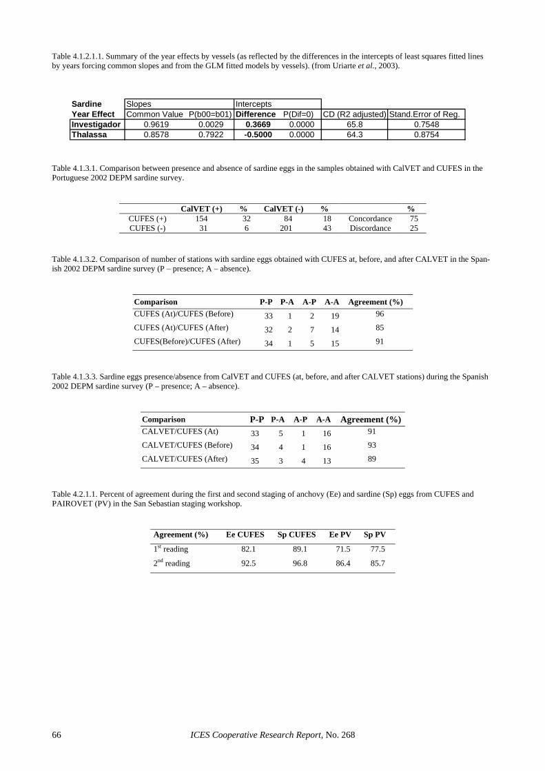
Table 4.1.2.1.1. Summary of the year effects by vessels (as reflected by the differences in the intercepts of least squares fitted lines by years forcing common slopes and from the GLM fitted models by vessels). (from Uriarte et al., 2003).
Sardine Slopes InterceptsYear Effect Common Value P(b00=b01) Difference P(Dif=0) CD (R2 adjusted) Stand.Error of Reg.Investigador 0.9619 0.0029 0.3669 0.0000 65.8 0.7548Thalassa 0.8578 0.7922 -0.5000 0.0000 64.3 0.8754
Table 4.1.3.1. Comparison between presence and absence of sardine eggs in the samples obtained with CalVET and CUFES in the Portuguese 2002 DEPM sardine survey.
CalVET (+) % CalVET (-) % % CUFES (+) 154 32 84 18 Concordance 75 CUFES (-) 31 6 201 43 Discordance 25
Table 4.1.3.2. Comparison of number of stations with sardine eggs obtained with CUFES at, before, and after CALVET in the Span-ish 2002 DEPM sardine survey (P – presence; A – absence).
Comparison P-P P-A A-P A-A Agreement (%) CUFES (At)/CUFES (Before) 33 1 2 19 96
CUFES (At)/CUFES (After) 32 2 7 14 85
CUFES(Before)/CUFES (After) 34 1 5 15 91
Table 4.1.3.3. Sardine eggs presence/absence from CalVET and CUFES (at, before, and after CALVET stations) during the Spanish 2002 DEPM sardine survey (P – presence; A – absence).
Comparison P-P P-A A-P A-A Agreement (%) CALVET/CUFES (At) 33 5 1 16 91
CALVET/CUFES (Before) 34 4 1 16 93
CALVET/CUFES (After) 35 3 4 13 89
Table 4.2.1.1. Percent of agreement during the first and second staging of anchovy (Ee) and sardine (Sp) eggs from CUFES and PAIROVET (PV) in the San Sebastian staging workshop.
Agreement (%) Ee CUFES Sp CUFES Ee PV Sp PV
1st reading 82.1 89.1 71.5 77.5
2nd reading 92.5 96.8 86.4 85.7
ICES Cooperative Research Report, No. 268 66
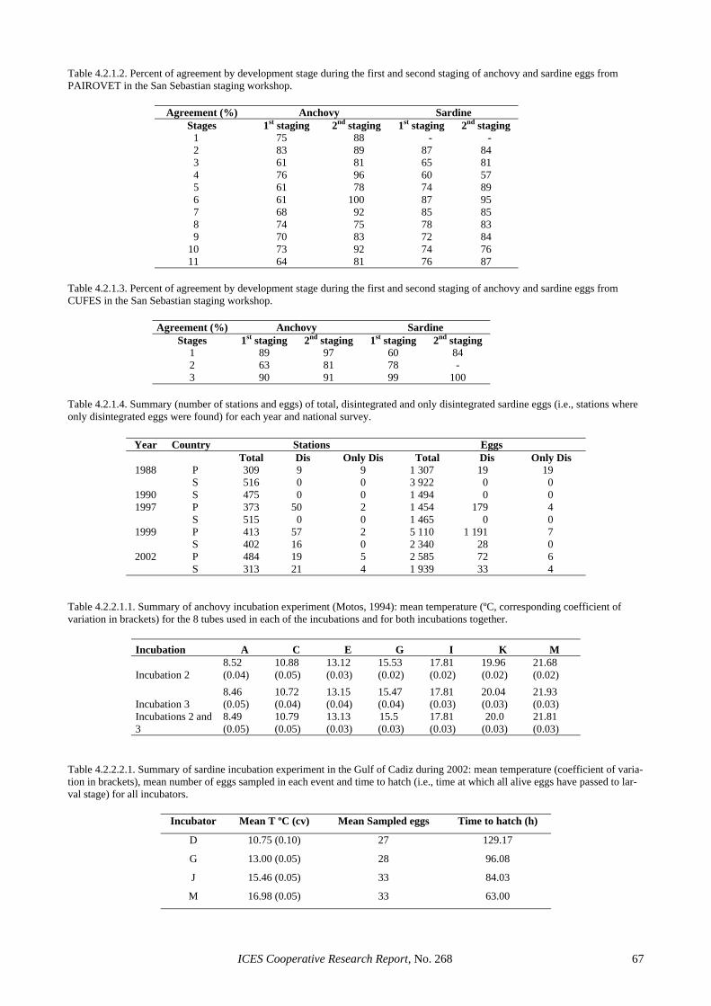
Table 4.2.1.2. Percent of agreement by development stage during the first and second staging of anchovy and sardine eggs from PAIROVET in the San Sebastian staging workshop.
Agreement (%) Anchovy Sardine Stages 1st staging 2nd staging 1st staging 2nd staging
1 75 88 - - 2 83 89 87 84 3 61 81 65 81 4 76 96 60 57 5 61 78 74 89 6 61 100 87 95 7 68 92 85 85 8 74 75 78 83 9 70 83 72 84
10 73 92 74 76 11 64 81 76 87
Table 4.2.1.3. Percent of agreement by development stage during the first and second staging of anchovy and sardine eggs from CUFES in the San Sebastian staging workshop.
Agreement (%) Anchovy Sardine Stages 1st staging 2nd staging 1st staging 2nd staging
1 89 97 60 84 2 63 81 78 - 3 90 91 99 100
Table 4.2.1.4. Summary (number of stations and eggs) of total, disintegrated and only disintegrated sardine eggs (i.e., stations where only disintegrated eggs were found) for each year and national survey.
Year Country Stations Eggs Total Dis Only Dis Total Dis Only Dis
1988 P 309 9 9 1 307 19 19 S 516 0 0 3 922 0 0
1990 S 475 0 0 1 494 0 0 1997 P 373 50 2 1 454 179 4
S 515 0 0 1 465 0 0 1999 P 413 57 2 5 110 1 191 7
S 402 16 0 2 340 28 0 2002 P 484 19 5 2 585 72 6
S 313 21 4 1 939 33 4 Table 4.2.2.1.1. Summary of anchovy incubation experiment (Motos, 1994): mean temperature (ºC, corresponding coefficient of variation in brackets) for the 8 tubes used in each of the incubations and for both incubations together.
Incubation A C E G I K M
Incubation 2 8.52 (0.04)
10.88 (0.05)
13.12 (0.03)
15.53 (0.02)
17.81 (0.02)
19.96 (0.02)
21.68 (0.02)
Incubation 3 8.46 (0.05)
10.72 (0.04)
13.15 (0.04)
15.47 (0.04)
17.81 (0.03)
20.04 (0.03)
21.93 (0.03)
Incubations 2 and 3
8.49 (0.05)
10.79 (0.05)
13.13 (0.03)
15.5 (0.03)
17.81 (0.03)
20.0 (0.03)
21.81 (0.03)
Table 4.2.2.2.1. Summary of sardine incubation experiment in the Gulf of Cadiz during 2002: mean temperature (coefficient of varia-tion in brackets), mean number of eggs sampled in each event and time to hatch (i.e., time at which all alive eggs have passed to lar-val stage) for all incubators.
Incubator Mean T ºC (cv) Mean Sampled eggs Time to hatch (h)
D 10.75 (0.10) 27 129.17
G 13.00 (0.05) 28 96.08
J 15.46 (0.05) 33 84.03
M 16.98 (0.05) 33 63.00
ICES Cooperative Research Report, No. 268 67
68 IC
ES Cooperative Research Report, N
o. 268
Table 4.3.1.1. Macroscopic and microscopic maturity scale for female sardine.
MATURITY STAGE MACROSCOPIC DESCRIPTION MICROSCOPIC DESCRIPTION
I VIRGIN AND RESTING Invisible or very small cord-shaped ovaries; translucent with almost no colour.
Unyolked oocytes as the unique type of oocytes present in the gonad.
II DEVELOPING Wider ovaries occupying 1/4 to 3/4 of body cavity; opaque with pinkish or yellow colour . Visible oocytes are not present.
The most advanced batch of oocytes are partially-yolked ones.
III PRE-SPAWNING Bigger ovaries occupying 3/4 to almost fitting body cavity; opaque with yellow or orange colour . Small opaque oocytes are visible.
The most advanced batch of oocytes are yolked ones.
IV SPAWNING Large ovaries occupying the full body cavity; fully or partially translucent with gelatinous aspect. Hyaline oocytes are visible (some small opaque oocytes can be visible).
The most advanced batch of oocytes are hydrated ones.
V PARTIAL POST-SPAWNING (recovering to Stage III)
Deflated and flaccid ovaries occupying about 3/4 of body cavity; with some ruptured blood vessels that gives them a bloodshot aspect. Some small opaque oocytes are visible (some hyaline oocytes can be pre-sent).
Post-ovulatory Follicles may be present. Some ruptured blood vessels and free haemocytes present spread all over the ovary tissue (light haemocyte infiltration). Presence of all oocyte stages is possible.
VI ULTIMATE POST-SPAWNING
Very deflated and flaccid ovaries occupying from about 3/4 to 1/4 of body cavity; with many ruptured blood vessels that gives them a reddish colour. Some small opaque oocytes can be visible (no hyaline oocytes are present)
Post-ovulatory Follicles may be present. Many ruptured blood vessels and free haemocytes invading the ovary tissue (generalised haemocyte infiltration). No yolked oocytes, or most of them in an atretic state.
Table 4.3.1.2.1. Correspondence (%) between macroscopic and microscopic classifications of female sardine maturity (data collected during the November 2000 Portuguese acoustic survey).
I II III IV V V-III NStage I 75.5 24.5 49Stage II 6.7 60.0 20.0 6.7 6.7 15Stage III 50.0 50.0 6Stage IV 4.2 95.8 24Stage V 36.4 27.3 0.0 36.4 11
Stage V-III 56.9 5.6 37.5 72
Macroscopic maturity stage
Microscopic maturity stage
Table 4.3.1.2.2. Correspondence (%) between macroscopic and microscopic classifications of female sardine maturity in DEPM sur-veys (in 1999, the macroscopic stages were attributed to formol-fixed, instead of fresh, gonads).
I II III IV NI 0II 66 28 7 61III 3 4 92 2 253IV 3 0 3 93 30V 0
V-III 1 99 116I 38 13 50II 26 9 65 23III 1 1 93 6 563IV 24 76 42V 0
V-III 0I 100 1II 50 33 17 6III 100 12IV 2 98 129V 22 51 28
V-III 5 95 361
Microscopic maturity stage
March 1997
January 1999
January 2002
Macroscopic maturity stageSurvey
8
65
ICES Cooperative Research Report, No. 268 69
- SARDINE - Investigador log-log plot
01122334455
0 1 2 3 4 5Cufes BA m ean
Cuf
es o
n st
atio
n20002001Linea 1:1
Figure 4.1.2.1.1. Comparison of CUFES sardine egg densities (eggs/m3, log-scale) in underway (before and after the PAIROVET haul - CUFES BA mean) and stationary (4 min during the PAIROVET haul (CUFES on station) samples from two years (2000 and 2001). Line is 1:1 relationship and encircled points are removed outliers (from Uriarte et al., 2003).
Figure 4.1.2.2.1. Example of vertical egg distribution fitting to the average of LHPR hauls from the sampling in 2000 and 2001 for anchovy in waters of high salinity at surface (Boyra et al., in press).
ICES Cooperative Research Report, No. 268 70
Figure 4.1.2.2.2. Example of vertical egg distribution fitting to the average of LHPR hauls from the sampling in 2000 and 2001 for anchovy in waters of low salinity at surface (Boyra et al., in press).
0%
10%
20%
30%
40%
50%
60%
Allstages
Day-1 Day-2 Day-3 Dis
Pres
ence
of e
ggs
CalVETCUFES
Figure 4.1.3.1. Comparison of the proportion of stations where sardine eggs (all stages and separately by broad categories of devel-opment) were detected by CalVET (blue columns) and CUFES (red columns) during the 2002 Portuguese DEPM survey.
ICES Cooperative Research Report, No. 268 71
0%
10%
20%
30%
40%
50%
60%
I II III DisStages
CalVET CUFES
Figure 4.1.3.2. Percentage of sardine eggs at stage (broad stages for CUFES applications) in CalVET and CUFES in the calibration exercise performed during the Spanish 2002 DEPM survey.
0%
10%
20%
30%
40%
50%
I II III IV V VI VII VIII IX X XI Dis
Stages
CalVET CUFES
Figure 4.1.3.3. Percentage of sardine eggs at stage (standard stages for DEPM applications) in CalVET and CUFES in the calibration exercise performed during the Spanish 2002 DEPM survey.
Figure 4.1.4.1. Distribution of two daily cohorts of sardine eggs (hatched during the night of sampling in the left and 1 night before in the right) within a restricted area (approximately 120 nm2) in the Gulf of Cadiz. Circles indicate egg presence (with radius propor-tional to egg density) and crosses egg absence.
ICES Cooperative Research Report, No. 268 72
2 4 6 8 10 12
020
4060
8010
0
T emp 8.49
Stage
Age
(h)
2 4 6 8 10 12
020
4060
8010
0
Temp 10.79
Stage
Age
(h)
2 4 6 8 10 12
02
04
06
08
01
00
T em p 1 3 .1 3
S tage
Ag
e(h
)
2 4 6 8 10 12
020
4060
8010
0
T e m p 1 5 .5
S tage
Ag
e(h
)
2 4 6 8 1 0 1 2
02
04
06
08
01
00
T e m p 1 7 .8 1
S ta g e
Ag
e(h
)
2 4 6 8 1 0 1 2
02
04
06
08
01
00
T e m p 2 0
S ta g e
Ag
e(h
)
Figure 4.2.2.1.1. Observed age (in hours) for each stage and temperature (data from anchovy incubation experiment).
ICES Cooperative Research Report, No. 268 73
2 4 6 8 10
020
4060
8010
012
014
0
Stage
Age
8.4910.7913.1315.517.812021.81
Figure 4.2.2.1.2. Mean age vs. stage from Lo’s model fitted to anchovy incubation experiment data. Each line represents a different incubation temperature.
ICES Cooperative Research Report, No. 268 74
0 20 40 60 80 100
0.0
0.2
0.4
0.6
0.8
1.0
Temp 13.13
time (hours)
P[s
tage
]
0 20 40 60 80 100
0.0
0.2
0.4
0.6
0.8
1.0
Temp 15.5
time (hours)
P[s
tage
]
0 20 40 60 80 100
0.0
0.2
0.4
0.6
0.8
1.0
Temp 10.79
time (hours)
P[s
tage
]
0 20 40 60 80 100
0.0
0.2
0.4
0.6
0.8
1.0
Temp 8.49
time (hours)
P[s
tage
]
2
22222
2
2
2
22222222 2222 2 22 22 222222 222
2 2
2222233333333 3333 3 33 33 333333 3333
3
3
33
3
33
3
3
3
33333444444444444 44 444 4 44 44 444444 4444
4
4
4
4
4
444445555555555555555 5 5 55 55 555555 5555
5
5
55
5
55555666666666666666666 666 6 66 666666 6666
6
6
6
66666777777777777777777 7777 7 7 7 77777 7777
7 7 7
77777888888888888888888 8888 8 88 8 8 88 8888
8
8
8
8
88888999999999999999999 9999 9 99 99 9
99
9999
9
9
9
9
9
9
99aaaaaaaaaaaaaaaaaa aaaa a aa aa aaaaaa
a
a
a
a
a
a
aaa
2
2
2222
2
22
2
22
22
2
2
2 22 22 2 22 22 22 22222222 222 22 2 2 2
2
2 2 2333333 33 33 3 33 33 33 33333333 333 33 3 3 33
3
3
33
3
3
3
3
3
3 3
3 3 344444444444444444 4 44 4 4 44444444 444 44 4 4 44
4 4
4
4 4
4
4 4 455555555555555555 55 55 5 5 5555555 555 55 5 5 55
55
5
5
5
5
5 5 566666666666666666 66 66 6 66 66 6 666 66 6 6 66
6
6
66
6
6
6
6
6
6 6 677777777777777777 77 77 7 77 77 77 777 77 7 77 7 7 77
7
7
7
7
7
7 7 788888888888888888 88 88 8 88 88 88 88888888 8 8 88
8
8
88
8
8 8 899999999999999999 99 99 9 99 99 99 99999999 999 99
9
99
9
9
9 9aaaaaaaaaaaaaaaaa aa aa a aa aa aa aaaaaaaa aaa aa a a
a
a
a
a
a
2
22
2 2
2
22
2 22
2
2 22
2
2 22 22
2
22222 2 222
2 2
3 33 333 3 3 3333 3 3 3 33
3 3
3
3 33 3 3
3 3
33 3 33 3
4 444 444444 44 4 4 4 4 44 444444 444
4
4
4 4
4
4
5 555 555555 55 5 5 55 5 55 5 5 555 5 5555
5
5
5
5
6 666 666666 66 6 6 66 66 66 666 666 66
66
6
6
6
7 777 777777 77 7 7 77 77 77 77777777 7 77778 888 888888 88 8 8 88 88 88 88888888 8 88889 999 999999 99 9 9 99 99 99 99999999 9 9999a aaa aaaaaa aa a a aa aa aa aaaaaaaa a aaaa
2
2
2
22222
2
222 2 22 2 22 22222 2 2 2 2 2
2
3 3 3 3 3 33 3 3 3 3 33
3
33333
3
333 3 3
3
3 3 3
4 4 4 444444 444 4 4 44 44444 4 4 4 4 44
4
4
5 5 5 555555 555 5 55 5 5 5 55 5 5 5 55
5 5 5
5
6 6 6 666666 666 6 66 6 66 66666
6 6
6
6 6 6
7 7 7 777777 777 7 77 7 77 77777 7 7 7 7 778 8 8 888888 888 8 88 8 88 88888 8 8 8 8 889 9 9 999999 999 9 99 9 99 99999 9 9 9 9 99a a a aaaaaa aaa a aa a aa aaaaa a a a a aa
0 20 40 60 80 100
0.0
0.2
0.4
0.6
0.8
1.0
Temp 17.81
time (hours)
P[s
tage
]
0 20 40 60 80 100
0.0
0.2
0.4
0.6
0.8
1.0
Temp 20
time (hours)
P[s
tage
]
0 20 40 60 80 1000.
00.
20.
40.
60.
81.
0
Temp 21.81
time (hours)
P[s
tage
]
2
2222
2
22
2
22 222222 22 22 2 22 22 222 22
2 2
2
333333 3 3333 33 33 3 33 33 333 333
3
33
3
33 3
3
444444444444 4 444 44 44 4 44 44 444 444
4
4
4
555555555555555 55 55 5 55 55 555 555
5
55
5
666666666666666666 6 6 66 66 666 666
6
66
6
7777777777777777777 77 77 77 777 777
7
7
7
8888888888888888888 88 88 8 88 888 888
8
8
9999999999999999999 99 99 9
9
9 9 999
9
9
99
aaaaaaaaaaaaaaaaaaa aa aa a aa a
a
a
a
a
a
aa
2
22222
22
2
222222222 222 2 2
2
2
2
3333333 33333 333 3 33
3
33
3
3
3
3
3
44444444444 4444444 444 4 44
4
4
5555555555555 5555 555 5 55
5
5
5
6666666666666666 6 666 6 66
666
7777777777777777777 77 7 77
7
7
8888888888888888888 8 8 88
8
8
8
99999999999999999999 99 9 99
9
aaaaaaaaaaaaaaaaaaaa aaa
a
aa
2
22222
2
222222222222 222 2
2
333333 3333333 333 33
3
3
333
3
44444444 44444444 444 44
444
55555555555 55555 555 55
5
5
5
6666666666666 66 666 66
6
66
6
7777777777777777 7 7777
7
7
7888888888888888888 88 88
8
8
9999999999999999999 99 99
9
aaaaaaaaaaaaaaaaaaa a
a
a
a
a
1
3456789
b
IIIIIIIVVVIVIIVIIIIXXXI
2
a
Figure 4.2.2.1.3. Probability of being at stage along observation time (age) from models fitted to anchovy incubation data (one incubation temperature in each panel).
IIIIIIIVVVIVIIVIIIIXXXI
IC
ES Cooperative Research Report, N
o. 268 75
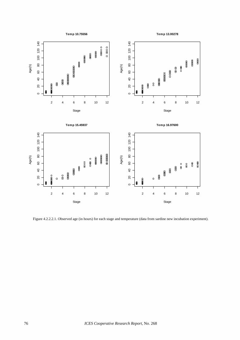
2 4 6 8 10 12
020
4060
8010
012
014
0Temp 10.75556
Stage
Age(
h)
2 4 6 8 10 12
020
4060
8010
012
014
0
Temp 13.00278
Stage
Age(
h)
2 4 6 8 10 12
020
4060
8010
012
014
0
Temp 15.45937
Stage
Age(
h)
2 4 6 8 10 12
020
4060
8010
012
014
0Temp 16.97600
Stage
Age(
h)
Figure 4.2.2.2.1. Observed age (in hours) for each stage and temperature (data from sardine new incubation experiment).
ICES Cooperative Research Report, No. 268 76
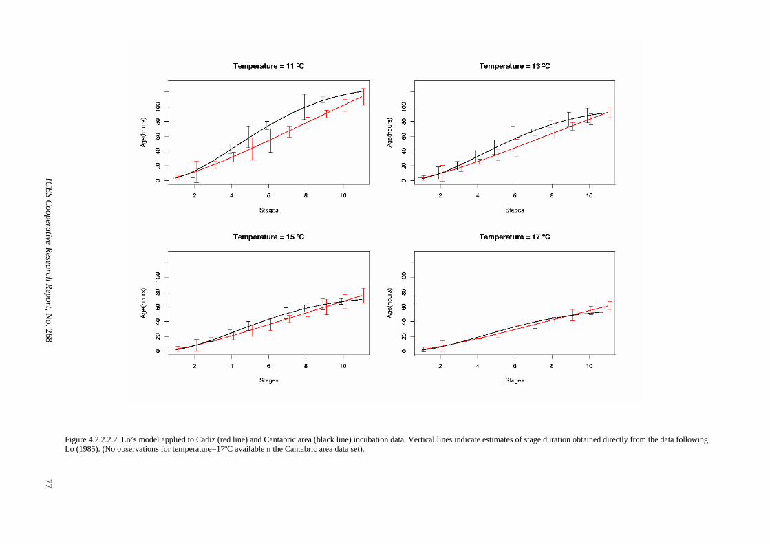
IC
ES Cooperative Research Report, N
o. 268 77
Figure 4.2.2.2.2. Lo’s model applied to Cadiz (red line) and Cantabric area (black line) incubation data. Vertical lines indicate estimates of stage duration obtained directly from the data following Lo (1985). (No observations for temperature=17ºC available n the Cantabric area data set).
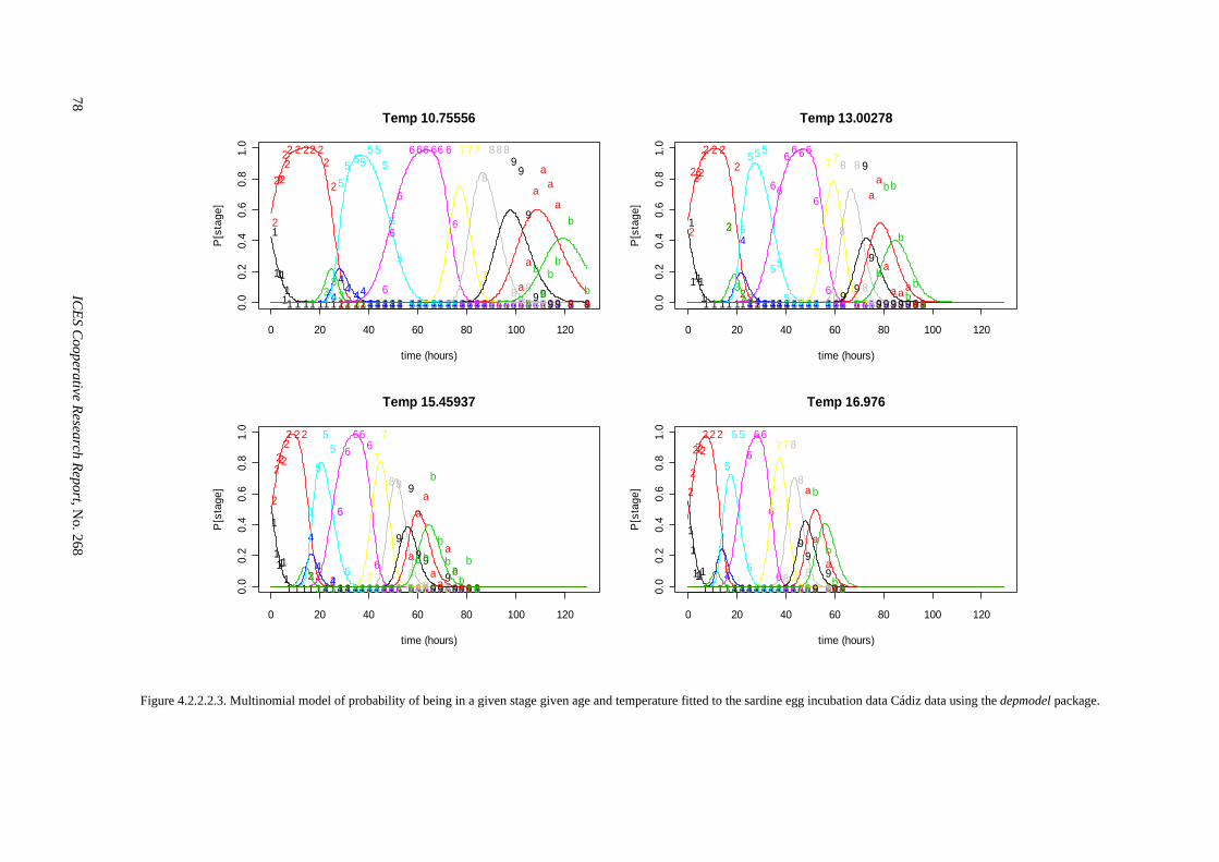
Figure 4.2.2.2.3. Multinomial model of probability of being in a given stage given age and temperature fitted to the sardine egg incubation data Cádiz data using the depmodel package.
0 20 40 60 80 100 120
0.0
0.2
0.4
0.6
0.8
1.0
Temp 10.75556
time (hours)
P[s
tage
]1
111
111 1 11 111 11 111 111 1 1 11 11 111 11 111 111 11 111 1 1
2
222
222 2 22 2
2
2
22 222 222 2 2 22 22 222 22 222 222 22 222 2 23
33
3 333 333 3 3 33 33 333 33 333 333 33 333 3 344
4 444 444 4 4 44 44 444 44 444 444 44 444 4 45
55 55
5 55
5
5
5 55 55 555 55 555 555 55 555 5 56
6
6
6 66 66 6
6
6 66 666 666 66 666 6 6
7
7 77
7
77 777 77 777 7 7
8
88 8
888
8 888 8 8
99
9
9 999 9 9
a
a
a
aa
a
a a
b
b
bb
b
bb
0 20 40 60 80 100 120
0.0
0.2
0.4
0.6
0.8
1.0
Temp 13.00278
time (hours)
P[s
tage
]
1
111111 1 11 11 111 111 11 11 1111 1 11 111 11 11
2
222222 2 2
2
2
2222 222 22 22 2222 2 22 222 22 22
3
33 333 333 33 33 3333 3 33 333 33 33
4
44 4 444 44 44 4444 4 44 444 44 44
5
555
55
5 55 55 5555 5 55 555 55 55
66
6 66 6
6
6666 6 66 666 66 667
7
77
7
77 77 777 77 77
8
8
8 8
88 888 88 88
99
9
9
999 99 99
aa
a
a aaaa
b
bb
b
bb
b
0 20 40 60 80 100 120
0.0
0.2
0.4
0.6
0.8
1.0
Temp 15.45937
time (hours)
P[s
tage
]
1
1111
11 1 111 11 1 1 11 11 111 1 11 111 111 1
2
2222
22 2 2
22 22 2 2 22 22 222 2 22 222 222 2
33 33 3 3 33 33 333 3 33 333 333 3
4
44
4 4 4 44 44 444 4 44 444 444 4
5
5
55
5
555 55 555 5 55 555 555 5
6
666
6
6
666 6 66 666 666 67
7
7
7
7 7 77 777 777 7
88
888 888 888 8
9
9
9 99
99 999 9
a
aa
aa
a
aaa a
b b
b
b
bb
b
b
b b
0 20 40 60 80 100 120
0.0
0.2
0.4
0.6
0.8
1.0
Temp 16.976
time (hours)P
[sta
ge]
1
1
111111 111 11 111 111 11 11 11
2
2
222222 2
2
2 22 222 222 22 22 2233 33 333 333 33 33 334
4 44 444 444 44 44 44
5
5 5
5
555 555 55 55 55
6
66
6
666 66 66 66
7
77
777 77 77
8
8
8
888 88
99
99 99
a
a
a
aa
b
b
bb b
78 IC
ES Cooperative Research Report, N
o. 268
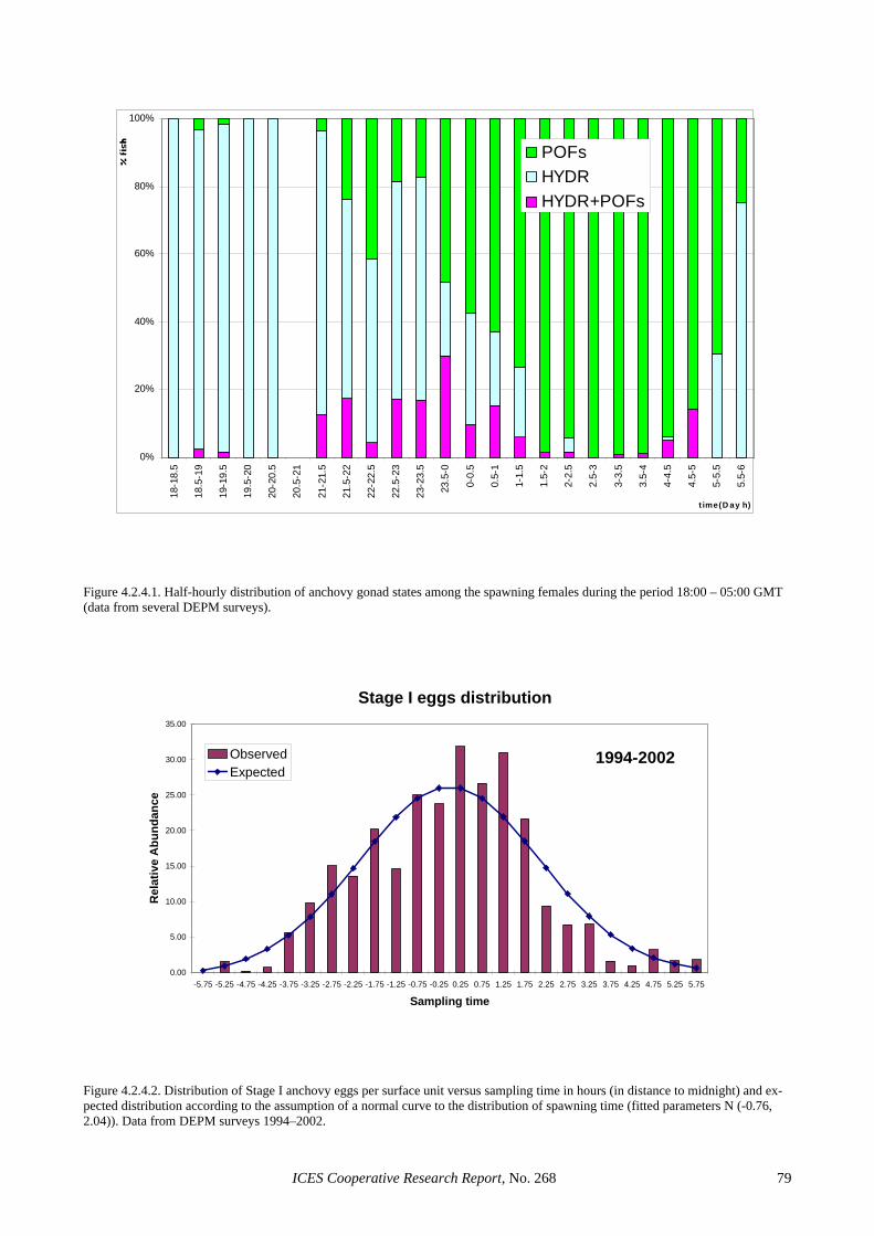
0%
20%
40%
60%
80%
100%
18-1
8.5
18.5
-19
19-1
9.5
19.5
-20
20-2
0.5
20.5
-21
21-2
1.5
21.5
-22
22-2
2.5
22.5
-23
23-2
3.5
23.5
-0
0-0.
5
0.5-
1
1-1.
5
1.5-
2
2-2.
5
2.5-
3
3-3.
5
3.5-
4
4-4.
5
4.5-
5
5-5.
5
5.5-
6
t ime(D ay h)
POFsHYDRHYDR+POFs
Figure 4.2.4.1. Half-hourly distribution of anchovy gonad states among the spawning females during the period 18:00 – 05:00 GMT (data from several DEPM surveys).
Stage I eggs distribution
0.00
5.00
10.00
15.00
20.00
25.00
30.00
35.00
-5.75 -5.25 -4.75 -4.25 -3.75 -3.25 -2.75 -2.25 -1.75 -1.25 -0.75 -0.25 0.25 0.75 1.25 1.75 2.25 2.75 3.25 3.75 4.25 4.75 5.25 5.75
Sampling time
Rel
ativ
e A
bund
ance
ObservedExpected
1994-2002
Figure 4.2.4.2. Distribution of Stage I anchovy eggs per surface unit versus sampling time in hours (in distance to midnight) and ex-pected distribution according to the assumption of a normal curve to the distribution of spawning time (fitted parameters N (-0.76, 2.04)). Data from DEPM surveys 1994–2002.
ICES Cooperative Research Report, No. 268 79
Time of day (h)
Gon
ados
omat
ic In
dex
10 12 14 16 18
0.0
0.05
0.10
0.15
0.20
0.25
0.30
A
Time of day (h)
Ooc
yte
dens
ity (e
ggs
/ gra
m o
f gon
ad)
10 12 14 16 180
1000
2000
3000
4000
B
Figure 4.2.4.3. Diurnal development of gonadosomatic index (a) and hydrated oocyte density (b) for female sardines sampled during the day of anticipated spawning (from Zwolinski et al., 2001).
5 10 15 20
0.0
0.2
0.4
0.6
0.8
Sampling Time (h)
Spa
wni
ng d
ensi
ty
Figure 4.2.4.4. Proportion of stage I sardine eggs caught hourly during DEPM surveys (open circles) and during sampling in a fixed location (closed circles, data from Ré et al., 1988). Lines correspond to a normal density functions with a 22 hr. mean and standard deviation of 0.5 (thin continuous), 1 hr. (thick continuous) and 2 hr. (broken) respectively.
ICES Cooperative Research Report, No. 268 80
II DEVELOPING
III PRE-SPAWNING
IV SPAWNING
I VIRGIN AND RESTING
V PARTIAL POST-SPAWNING
(recovering to Stage III)
n times per spawning
season
VI ULTIMATE POST-SPAWNING
(recovering to Stage I)
1 time per spawning
season
Figure 4.3.1.1. Female Sardine Maturity Cycle (based on the scale of Table 3.3.1.1).
Figure 4.3.2.1.1. Proportion of active female sardines as a function of their gonadosomatic index (GSI) and respective ogive to iden-tify the value of GSI at which half of the sardine females are active (from Ganias, 2003).
ICES Cooperative Research Report, No. 268 81
0%
20%
40%
60%
80%
100%
Sep Oct Nov Dec Jan Feb Mar Apr May Jun Jul Aug
1999 2000
Late postspawning/immature Early postspawning Active
Figure 4.3.2.1.2. Evolution of the monthly fractions of active, early postspawning and late postspawning/immature female sardines in the Mediterranean (from Ganias et al., submitted).
05
1015
GSI, %
Sep Oct Nov Dec Jan Feb Mar Apr May
1998/19991999/20002000/20012001/2002
Figure 4.3.2.2.1. Average monthly female gonadosomatic index (GSI) along the sardine spawning season off Portugal in recent years (data from Portuguese market samples).
ICES Cooperative Research Report, No. 268 82
0%
20%
40%
60%
80%
100%
2/2
Sept
.
2/2
Oct
.
2/2
Nov
.
2/2
Dec
.
2/2
Jan.
2/2
Feb.
2/2
Mar
.
2/2
Apr
.
2/2
May
Freq
uenc
y of
mat
ure
fem
ales
(%)
Figure 4.3.2.2.2. Evolution of female sexual maturation at the northern (diamonds) and southern (black squares) coasts during 2001/2002 spawning season.
0.00
0.05
0.10
0.15
0.20
2/2
Sep
t.
2/2
Oct
.
2/2
Nov
.
2/2
Dec
.
2/2
Jan.
2/2
Feb.
2/2
Mar
.
2/2
Apr
.
2/2
May
Saw
ning
frac
tion
Figure 4.3.2.2.3. Temporal progression of spawning fraction along the northern (diamonds) and southern (squares) coasts during 2001/2002 spawning season.
ICES Cooperative Research Report, No. 268 83
5 References
Alheit, J. 1985. Spawning frequency of Peruvian anchovies taken with a purse seine. In An Egg Production Method for Estimating Spawning Biomass of Pelagic Fish: Appli-cation to the Northern Anchovy, Engraulis mordax, pp. 99–101. Ed. by R. Lasker. NOAA Technical Report, NMFS 36.
Alheit, J. 1993. Use of the Daily Egg Production Method for estimating biomass of clupeoid fishes: a review and evaluation. Bulletin of Marine Science, 53: 750–767.
Anonymous. 1997. Workshop on improvements of DEPM techniques. Ozeanografika, 2: 1–165.
Axelsen, B. E., Nottestad, L., Ferno, A., Johannessen, A., and Misund, O. A. 2000. “Await” in the pelagic: dynamic trade-off between reproduction and survival within a her-ring school splitting vertically during spawning. Marine Ecology Progress Series, 205: 259–269.
Bernal, M. 1999. Preliminary results on a two stage modeling of sardine egg presence and abundance off the Spanish coast and its implication for stock assessment. Working Document for the ICES Working Group on the Assess-ment of Mackerel, Horse Mackerel Sardine and Anchovy, Copenhagen, September 1999.
Bernal, M., Franco, C., Pérez, J. R., and Lago de Lanzós, A. 2000. DEPM estimates of sardine (Sardina pilchardus) SSB off the Spanish coast in 1999. Working Document presented at the Workshop on Sardine SSB Estimation, Vigo, 13–16 June 2000.
Bernal, M., Borchers, D. L., Valdés, L., Lanzós, A. L., and Buckland, S. T. 2001. A new ageing method for eggs of fish species with daily spawning synchronicity. Canadian Journal of Fisheries and Aquatic Sciences, 58: 2330–2340.
Bez, N. 2000. Comparing anchovy egg densities measured by CUFES and Vertical Plankton tows in the Bay of Biscay. In Checkley et al. (2000) pp 15–19.
Borchers, D. L., Buckland, S. T., Priede, I. G., and Ahmadi, S. 1997. Improving the precision of the daily egg production method using generalised additive models. Canadian Journal of Fisheries and Aquatic Sciences, 54: 2727–2742.
Boyra, G., Rueda, L. D., Coombs, S. H., Sunby, S., Ådlands-vik, B., Santos, M., and Uriarte, A. 2003. Modelling the vertical distribution of eggs of anchovy (Engraulis encra-sicolus) and sardine (Sardina pilchardus). Fisheries Oceanography, 12: 381–395.
Casavola, N. 1998. Daily egg production method for spawning biomass estimates of anchovy in the south-western Adri-atic during 1994. Rapports de la Communnité Internatio-nalle du mer Mediterranée, 35: 394–395.
Checkley, D. M., Ortner, P. B., Settle, L. R., and Cummings, S. R. 1997. A continuous, underway fish egg sampler. Fisheries Oceanography, 6: 58–73.
Checkley, D. M., Ortner, P. B., Werner, F. E., Settle, L. R., and Cummings, S. R. 1999a. Spawning habitat of the Atlantic menhaden in Onslow Bay, North Carolina. Fisheries Oceanography, 8: 22–36.
Checkley, D. M., Motos, L., Uriarte, A., Santos, M., Trivedi, M., and Iwamoto, S. 1999b. Continuous, underway sam-pling of pelagic fish eggs and the environment: the Bay of Biscay anchovy and machine vision research. ICES CM 1999/M:05.
Checkley, D. M., Hunter, J. R., Motos, L., and van der Lingen, L. D. 2000. (Eds.). Report of a workshop on the use of the Continuous Underway Fish Egg Sampler (CUFES) for mapping spawning habitats of pelagic fish. GLOBEC Report, 14: 1–65 pp. (and references therein).
Cochran, W. G. 1977. Sampling techniques. 3rd Edition. Wiley, New York.
Coombs, S. H., Fosh, C. A., and Keen, M. A. 1985. The buoy-ancy and vertical distribution of eggs of sprat (Sprattus sprattus) and pilchard (Sardina pilchardus). Journal of the Marine Biological Association UK, 65: 461–474.
Cunha, M. E., Figueiredo, I., Farinha, A., and Santos, M. 1992. Estimation of sardine spawning biomass off Portugal by the Daily Egg Production Method. Boletín del Instituto Español de Oceanografía, 8: 139–153.
Cunha, E., Farinha, A., and Soares, E. 1997. Preliminary esti-mation of sardine spawning biomass in ICES Division IXa (Lat. 41° 50´N, 36° 00´N) by the daily egg produc-tion method. Working Document for the ICES Working Group on the Assessment of Mackerel, Horse Mackerel Sardine and Anchovy, Copenhagen 9–18 September, 1997.
Drummond, C. D., Bazzoli, N., Rizzo, E., and Sato, Y. 2000. Post-ovulatory follicle: a model for experimental studies on programmed cell death and apoptosis in teleosts. Jour-nal of Experimental Zoology, 287: 176–182.
Eilers, P. H. C., and Marx, B. D. 1996. Flexible smoothing with B-splines and penalties (with discussion). Statistical Sci-ence, 11: 89–121.
Fitzhugh, R. G., and Hettler, F. W. 1995. Temperature influ-ence on postovulatory follicle degeneration in Atlantic menhaden, Brevoortia tyrannus. Fishery Bulletin, 93: 568–572.
Gamulin, T., and Hure, T. 1955. Contribution á la Conaissance de l’Ecologie de la Ponte de la Sardine (Sardina pilchar-dus, Walb.) dans l’Adriatique. Acta Adriatica, 7: 1–22.
Ganias, K. 2003. Oceanographic and biological study of sar-dine (Sardina pilchardus) plankton production off central Greece. PhD Thesis, University of Thessaly (in Greek with English abstract).
Ganias, K., Somarakis, S., Koutsikopoulos, C., Machias, A., and Theodorou, A. J. 2003a. Ovarian atresia in the Medi-terranean sardine, Sardina pilchardus sardina. Journal of Marine Biological Association, UK, 83: 1327–1332.
Ganias, K., Somarakis, S., Machias, A., and Theodorou, A. J. 2003b. Evaluation of spawning frequency in the Mediter-ranean sardine population (Sardina pilchardus sardina). Marine Biology, 142: 1169–1179.
Ganias, K., Somarakis, S., Machias, A., and Theodorou, A. J. 2004. Pattern of oocyte development and batch fecundity in the Mediterranean sardine. Fisheries Research 67: 13–23.
García, A., Pérez, N., Porteiro, C., and Carrera, P. 1991. Esti-mates of the sardine spawning stock biomass off the Galician and Cantarbian coasts. ICES CM 1991/H:35.
García, A., Pérez, N., Lo, N. C. H., Lago de Lanzos, A., and Sola, A. 1992. The Egg Production Method applied to the spawning biomass estimation of sardine, Sardina pil-chardus (Walb.) on the North Atlantic Spanish coast. Bo-letín del Instituto Español de Oceanografía, 8: 123–138.
García, A., Franco, C., Solá, A., and Lago de Lanzós, A. 1993. Producción diaria de huevos de sardina, Sardina pilchar-dus (Walb.), en las costas de Galicia, Cantabrico y golfo de Vizcaya, en Abril-Mayo, 1990. Boletín del Instituto Español de Oceanografía, 9: 237–250.
García, A., and Palomera, I. 1996. Anchovy early life history and its relation to its surrounding environment in the western Mediterranean basin. Scientia Marina, 60: 155–166.
Grilo, C. 2002. Evolution of sardine spawning fraction in two spawning areas of the Portuguese coast. Degree Thesis, University of Lisbon (in Portuguese).
Gu, C., and Wahba, G. 1991. Minimizing GCV/GML scores with multiple smoothing parameters via the Newton
ICES Cooperative Research Report, No. 268 84
method. SIAM Journal on Scientific and Statistical Com-puting, 12: 383–398.
Guisande, C., Riveiro, I., Solá, A., and Valdés, L. 1998. Effects of biotic and abiotic factors on the biochemical composi-tion of wildeggs and larvae of several fish species. Ma-rine Ecology Progress Series, 163: 53–61.
Hunter, J. R., and Macewicz, B. 1985. Measurement of spawn-ing frequency in multiple spawning fishes. In An Egg Production Method for Estimating Spawning Biomass of Pelagic Fish : Application to the Northern Anchovy, En-graulis mordax, pp. 79–93. Ed. by R. Lasker. NOAA Technical Report, NMFS 36:
Hunter, J. R., Lo, N. C. H., and Leong, J. H. 1985. Batch fe-cundity in multiple spawning fishes. In An Egg Produc-tion Method for Estimating Spawning Biomass of Pelagic Fish : Application to the Northern Anchovy, Engraulis mordax, pp. 67–77. Ed. by R. Lasker. NOAA Technical Report, NMFS 36.
Hunter, J. R. and Lo, N. C. H. 1997. The daily egg production method of biomass estimation : some problems and po-tential improvements. Ozeanografika, 2: 41–69.
ICES. 1982. Working Group for the Appraisal of Sardine Stocks in Divisions VIIIc and IXa. ICES CM 1982/Assess: 10.
ICES. 2000. Report of the Workshop on the Estimation of Spawning Stock Biomass of Sardine. ICES CM 2000/G:07.
ICES. 2002. Report of the Study Group on the Estimation of the Spawning Biomass of Sardine and Anchovy. ICES CM 2002/G:01.
ICES. 2003a. Report of the Working Group on the Assessment of Mackerel, Horse Mackerel, Sardine and Anchovy. ICES CM 2003/ACFM:07.
ICES. 2003b. Report of the Study Group on the Estimation of Spawning Stock Biomass for Sardine and Anchovy. ICES CM 2003/G:17.
Ihaka, R., and Gentleman, R. 1996. R: A language for data analysis and graphics. Journal of Computational and Graphical Analysis, 5: 299–314.
Lago de Lanzós, A., Quintanilla, L., and Franco, C. 1998. The daily egg production method applied to the spawning biomass estimation of sardine, Sardina pilchardus off the North Atlantic Spanish coast. ICES CM 1998/BB:17.
Laroche, J. L., and Richardson, S. L. 1980. Reproduction of northern anchovy, Engraulis mordax, off Oregon and Washington. Fishery Bulletin, 78: 603–618.
Lasker, R. 1985. (Ed.). An egg production method for estimat-ing spawning biomass of pelagic fish: application to the northern anchovy, Engraulis mordax. U.S. Department of Commerce. NOAA Technical Report, NMFS 36, 99 pp.
Lo, N. C. H. 1985. A model for temperature-dependent north-ern anchovy egg development and an automated proce-dure for the assignment of age to staged eggs. In An Egg Production Method for Estimating Spawning Biomass of Pelagic Fish: Application to the Northern Anchovy, En-graulis mordax. pp. 43–50. Ed. by R. Lasker. NOAA Technical Report, NMFS 36.
Lo, N. C. H., Hunter, J. R., and Charter, A. 2001. Use of a con-tinuous egg sampler for ichthyoplankton surveys: appli-cation to the estimation of daily egg production of Pacific sardine (Sardinops sagax) off California. Fishery Bulle-tin, 99: 554–571.
Macewicz, B., Castro Gonzalez, J. J., Cotero Altamirano, C. E., and Hunter, J. R. 1996. Adult reproductive parameters of Pacific sardine (Sardinops sagax) during 1994. California Cooperative Oceanic Fisheries Investigation Report, 37: 140–151.
MacGregor, J. S. 1957. Fecundity of the pacific Sardine (Sar-dinops caerulea). Fishery Bulletin, 57: 427–449.
Miranda, A., Cal, R. M., and Iglesias, J. 1990. Effect of tem-perature on the development of eggs and larvae of sardine Sardina pilchardus (Walbaum) in captivity. Journal of Experimental Marine Biology and Ecology, 140: 69–77.
Moser, H. G., and Ahlstrom, E. H. 1985. Staging anchovy eggs. In An Egg Production Method for Estimating Spawning Biomass of Pelagic Fish: Application to the Northern An-chovy, Engraulis mordax. pp 99–101. Ed. by R. Lasker. NOAA Technical Report, NMFS 36.
Motos, L. 1994 Estimación de la biomasa desovante de la po-blación de anchoa del golfo de vizcaya, Engraulis encra-sicolus, a partir de su producción de huevos. bases meto-dológicas y aplicación. PhD Thesis, Leioa, Spain.
Motos, L. 1996. Reproductive biology and fecundity of the Bay of Biscay anchovy (Engraulis Encrasicholus L.). Scientia Marina, 60.
Motos, L., and Uriarte, A. 1991. An egg production estimate of biomass of the Bay of Biscay Anchovy (Engraulis encra-sicholus L.) in 1990. ICES CM 1991/H:32.
Motos, L., and Uriarte, A. 1994. Assessing the Bay of Biscay anchovy using the DEPM during 1987–1992. Poster. Symposium on small and medium size pelagic fishes. Universidad Politécnica de Canarias, Facultad de Cien-cias del Mar. Las Palmas, January 1994.
Motos, L., Santiago, J., and Uriarte, A. 1991. Assessment of spawning biomass of the Bay of Biscay anchovy popula-tion, Engraulis encrasicholus L., using the daily egg pro-duction method. ICES CM 1991/H:33.
Olivar, M. P., Salat, J., and Palomera, I. 2001. Comparative study of spatial distribution patterns of the early stages of anchovy and pilchard in the NW Mediterranean Sea. Ma-rine Ecology Progress Series, 217: 111–120.
Palomera, I., and Pertierra, J. P. 1993. Anchovy spawning bio-mass estimate by the daily egg production method in 1990 in the western Mediterranean Sea. Scientia Marina, 57: 243–251.
Parker, R. L., and Rice, J. A. 1985. Discussion on “Some as-pects of the spline smoothing approach to non-parametric regression curve fitting” (by B.W. Silverman). Royal Sta-tistical Society Series B, 47: 40–42.
Parrish, R. H. et al. 1986. Age dependent fecundity, number of spawnings per year, sex ratio, and maturation stages in northern anchovy, Engraulis mordax. Fishery Bulletin, 84: 503–517.
Pépin, P. 1991 Effect of temperature and size on development, mortality and survival rates of the pelagic early life his-tory stages of marine fish. Canadian Journal of Fisheries and Aquatic Sciences, 48: 503–518.
Pérez, N., and Figueiredo, I. 1992. First approach to the study of atresia in the ovary of sardine, Sardina pilchardus (Walb.). Boletín del Instituto Español de Oceanografía, 8: 191–199.
Pérez, N., Figueiredo, I., and Macewicz, B. J. 1992a. The spawning frequency of sardine, Sardina pilchardus (Walb.), off the Atlantic Iberian coast. Boletín del Institu-to Español de Oceanografía, 8: 175–189.
Pérez, N., Figueiredo, I., and Lo, N. C. H. 1992b. Batch fecun-dity of sardine, Sardina pilchardus (Walb.), off the At-lantic Iberian coast. Boletín del Instituto Español de Oceanografía, 8: 155–162.
Picquelle, S. 1985. Sampling requirements for the adult fish surveys. In An Egg Production Method for Estimating Spawning Biomass of Pelagic Fish: Application to the Northern Anchovy, Engraulis mordax, pp. 55–57. Ed. by R. Lasker. NOAA Technical Report, NMFS 36.
Picquelle, S., and Stauffer, G. 1985. Parameter estimation for an egg production method of northern anchovy biomass assessment. In An Egg Production Method for Estimating Spawning Biomass of Pelagic Fish: Application to the
ICES Cooperative Research Report, No. 268 85
Northern Anchovy, Engraulis mordax, pp. 43–50. Ed. by R. Lasker. NOAA Technical Report, NMFS 36.
Pinto, J. S., and Andreu, B. 1957. Echelle pour la caractérisa-tion des phases evolutives de l’ovaire de sardine (Sardina pilchardus, Walb.) en rapport avec l’histophisiologie de la gonade. Proceedings of Technical Papers of the Gen-eral Fisheries Council for the Mediterranean, 4.
Poisson, F., and Massé, J. 2002. Report of the acoustic survey PELGAS02. Working Document to the ICES Working Group on the Assessment of Mackerel, Horse Mackerel, Sardine, and Anchovy. ICES CM 2002/ACFM:07.
Quintanilla, L., and Pérez, N. 2000a. Spawning frequency of sardine Sardina pilchardus (Walb.) off the Spanish North Atlantic coast in 1997. Fisheries Research, 45: 73–79.
Quintanilla, L., and Pérez, N. 2000b. Batch fecundity of sardine Sardina pilchardus (Walb.) off the Spanish North Atlan-tic coast in 1997. Working Document for the ICES Workshop on Sardine DEPM, Vigo, 16–19 June 2000.
Quintanilla, L., and García, A. 2001. Daily egg production method for estimating Sicilian Channel anchovy spawn-ing biomass in 1998 and 1999. Rapports de la Communi-té Internationalle du mer Mediterranée, 36: 7–15.
Ré, P., Farinha, A., and Meneses, I. 1988. Diel spawning time of sardine, Sardina pilchardus (Walbaum 1792) (Teleo-stei, Clupeidae), off Portugal. Investigación Pesquera, 52: 207–213.
Riveiro, I., Guisande, C., Lloves, M., Maneiro, I., and Cabanas, J. M. 2000. Importance of parental effects on larval sur-vival in Sardina pilchardus. Marine Ecology Progress Se-ries, 205: 249–258.
Smith ,P. E., and Hewitt, R. P. 1985. Sea survey design and analysis for an egg production method of anchovy bio-mass assessment. In An Egg Production Method for Es-timating Spawning Biomass of Pelagic Fish: Application to the Northern Anchovy, Engraulis mordax, pp. 17–26. Ed. by R. Lasker. NOAA Technical Report, NMFS 36.
Smith, P. E., Flerx, W., and Hewitt, R. P. 1985. The CalCOFI vertical egg tow (CalVET) net. In An Egg Production Method for Estimating Spawning Biomass of Pelagic Fish: Application to the Northern Anchovy, Engraulis mordax, pp. 27–32. Ed. by R. Lasker. NOAA Technical Report, NMFS 36.
Somarakis, S., Ganias, K., Koutsikopoulos, C., Machias, A., and Papaconstantinou, C. 2001. Applying the daily egg production method (DEPM) to small sardine stocks in the eastern Mediterranean. Working Document for the ICES Study Group on the Estimation of Spawning Stock Bio-mass for Sardine and Anchovy, Lisbon 22–25 October 2001. ICES CM 2001/G:01.
Somarakis, S., Koutsikopoulos, C., Machias, A., and Tsimenides, N. 2002. Applying the daily egg production method (DEPM) to small stocks in highly heterogeneous seas. Fisheries Research, 55: 193–204.
Steer, M. A., Moltschaniwsky, N. A., and Gowland, F. C. 2002. Temporal variability in embryonic development and mor-tality in the southern calamary Sepioteuthis australis: a field assessment. Marine Ecology Progress Series, 243: 143–150.
Stratoudakis, Y., Gallego, A., and Morrison, J. 1998. Spatial distribution of developmental egg ages within a herring (Clupea harengus) spawning ground. Marine Ecology Progress Series, 174: 27–32.
Stratoudakis, Y., and Fryer, R. J. 2000. Adult survey design and implications for sardine (Sardina pilchardus) DEPM estimation off Portugal. Working Document for the ICES Working Group on the Assessment of Mackerel, Horse Mackerel, Sardine and Anchovy. ICES CM 2001/ACFM:06.
Stratoudakis, Y., Soares, E., Garção, M., Mota, F., Albuquerque, J., Godinho, S., Morais, D., and Cunha, E.
2000. DEPM estimate of sardine spawning biomass in the area 36o – 41o 50´N during January 1999. Working Document for the ICES Workshop on Sardine DEPM, Vigo 16–19 June 2000.
Stratoudakis, Y., Lopes, P., Vicente, M. J., Figueiredo, A. S., and Marques, V. 2001. First comparison among CALVET, stationary and underway CUFES samplers si-multaneously used during the Portuguese PELASSES survey of March 2000. Working Document for the PELASSES meeting, Lisbon 12–16 February 2001.
Stratoudakis, Y., Bernal, M., Borchers, D., and Borges, M. F. 2003. Changes in the distribution of sardine eggs and lar-vae off Portugal, 1985–2000. Fisheries Oceanography, 12: 49–60.
Sundby, S. 1983 A one dimensional model for the vertical dis-tribution of pelagic fish eggs in the mixed layer. Deep-Sea Research, 30: 645–661
Sundby, S. 1991. Factors affecting the vertical distribution of eggs. ICES Marine Science Symposia, 192: 33–38.
Tsimenides, N., Somarakis, S., Magoulas, A., and Tserpes, G. 1995. Evaluation of the anchovy stocks in the Aegean Sea. Research Study MED/91/011. Final report. 58pp.
Uriarte, A. 2001.Anchovy population at age estimates and vari-ances for the application of the daily egg production method. ICES CM 2001/P:25.
Uriarte, A., Prouzet, P., and Villamor, B. 1996.Bay of Biscay and Ibero-Atlantic anchovy populations and their fisher-ies. Scientia Marina, 60: 237–255.
Uriarte, A., and Motos, L. 1998. Sampling errors in anchovy egg abundance estimates using the Pairovet net. Journal of Plankton Research, 20: 1861–1888.
Uriarte, A., Motos, L., Alvarez, P., Santos, M., Prouzet, P., and Massé, J. 1998. Population estimates of the Bay of Biscay anchovy in 1997 using the Daily Egg Production Method. Annex to the Interim Progress Report to European Com-mission of Project 96/034.
Uriarte, A., Motos, L., Alvarez, P., Santos, M., Prouzet, P., and Massé, J. 1999a. Population estimates of the Bay of Bis-cay anchovy by the Daily Egg Production Method. Final Report to European Commission of Project 96/034.
Uriarte, A., Motos, L., Santos, M., Alvarez, P., and Prouzet, P. 1999b. Assessment update for the Bay of Biscay An-chovy (Engraulis encrasicholus). Spawning biomass in 1995, 1996, 1997, 1998 and preliminary results of the 1999 survey. Working Document for the ICES Working Group on the Assessment of Mackerel, Horse Mackerel, Sardine and Anchovy. ICES, CM 2000/ACFM:05.
Uriarte, A., Santos, M., and Ibaibarriaga, L. 2003. Direct com-parison of the catching efficiency of CUFES and PAIROVET sampling for anchovy (Engraulis encrasico-lus) and sardine (Sardina pilchardus) eggs in the Bay of Biscay. AZTI Contribution to the final report Project 99/010 for the Commission of the European Community.
Vallin, L., and Nissling, A. 2000. Maternal effects on egg size and egg buoyancy of Baltic cod, Gadus morhua. Implica-tions for stock structure effects on recruitment. Fisheries Research, 49: 21–37.
Verea, M., Guisande, C., Riveiro, I., and Soler, I. 1997. Rela-tionships between protein, carbohydrate and lipid content with size in Atlantic horse mackerel (Trachurus trachu-rus), Altantic sardine (Sardina pilchardus) and Atlantic anchovy (Engraulis encrasicolus) larvae. Ichthyological Ecology, 47.
Ward, M. T., Hoedt, F., McLeay, M., Dimmlich, F. D., Kinloch, M., Jackson, G., McGarvey, J. P., Rogers, P. J., and Jones, K. 2001. Effect of the 1995 and 1998 mass mortality events on the spawning biomass of sardine, Sardinops sagax, in South Australian Waters. ICES Jour-nal of Marine Science, 58: 865–875.
ICES Cooperative Research Report, No. 268 86
Van der Lingen, C. D., Checkley, D., Barange, M., Hutchings, L., and Osgood, K. 1998. Assessing the abundance and distribution of eggs of sardine, Sardinops sagax, and round herring, Etrumeus whiteheadi, on the western Agulhas Bank, South Africa, using a continuous, under-way fish egg sampler. Fisheries Oceanorgaphy, 7: 35–47.
Wahba, G. 1980. Spline bases, regularization, and generalized cross validation for solving approximation problems with large quantities of noisy data. In Approximation Theory III. Ed. by W. Cheney. Academic Press, New York.
West, G. 1990. Methods of assessing ovarian development in fishes: a review. Australian Journal of Freshwater Re-search, 41: 199–222.
Williams R, Collins, N. R., and Conway, D. V. P. 1983. The double LHPR system, a high speed micro- and macroplankton sampler. Deep-See Research, 30: 331–342.
Wood, S. N. 2000. Modelling and smoothing parameter estima-tion with multiple quadratic penalties. Journal of the Royal Statistical Society (B), 62: 413–428.
Wood, S. N. 2003. Thin plate regression splines. Journal of the Royal Statistical Society (B), 65: 95–114.
Zwolinski, J. 2003. Small-scale spatial distribution of sardine eggs. MSc Thesis. Technical University of Lisbon (in Por-tuguese).
Zwolinski, J., Stratoudakis, Y., and Soares, E. 2001. Intra-annual variation in the batch fecundity of sardine off Portugal. Journal of Fish Biology, 58: 1633–1645.
ICES Cooperative Research Report, No. 268 87
6 Annexes
Annex I: Reference collection of sardine (Sardina pilchardus) egg stages. Staging based on Ahlstrom (1943).
Stage I
Stage II
blastodermalcap
Stage III
germinalring
Stage IV
embryo
Stage V
not optic vesicles
Stage VI
opticvesicls
Stage VII
the tail beginsto separate
Stage VIII
the tail is free for a length greater than the length ofthe head (about 1/3 of the body)
Stage IX
Stage X
the plane oforientation hasbeen rotated acomplete 90º
Stage XI
ICES Cooperative Research Report, No. 268 88
Annex II: Reference collection of anchovy (Engraulis encrasicolus) egg stages. Staging based on Moser, and Ahlstrom (1985).
Stage I
single cell
Stage II
start cell division
mulberrystage
Stage III
blastodermalcap
Stage IV
1/3
2/3
Stage V
> 2/3
Stage VI
clausure of theblastopore
Stage VII
the tailsbegind toseparate
Stage VIII
greater than 1/2head length
Stage IX
end of the tail
1/4
Stage X
1/2
Stage XI
3/4
ICES Cooperative Research Report, No. 268 89
Annex III: Reference collection of sardine (Sardina pilchardus) POF daily cohorts.
Sardine Day-0
Sardine Day-0
Sardine Day-0
Sardine Day-1
Sardine Day-1
Sardine Day-1
Sardine Day-2
Sardine Day-2
Sardine Day-2
Sardine Day-3
Sardine Day-3
Sardine Day-3
ICES Cooperative Research Report, No. 268 90
Annex IV: Reference collection of anchovy (Engraulis encrasicolus) POF daily cohorts.
Anchovy Day-0
Anchovy Day-1
Anchovy Day-2
Anchovy Day-3
ICES Cooperative Research Report, No. 268 91
Titles Published in the ICES Cooperative Research Report Series
No. Title Price (Danish Kroner)
269 The Annual ICES Ocean Climate Status Summary 2003/2004. 32 pp. 60
268 The DEPM Estimation of Spawning-stock Biomass for Sardine and Anchovy. 87 pp. In press
267 Report of the Thirteenth ICES Dialogue Meeting: Advancing scientific advice for an ecosystem ap-proach to management: collaboration amongst managers, scientists, and other stakeholders. 59 pp.
50
266 Mesh Size Measurement Revisited. 56 pp. 80
265 Trends in important diseases affecting the culture of fish and molluscs in the ICES area 1998–2002. 26 pp.
40
264 Alien Species Alert: Rapana venosa (veined whelk). 14 pp. 50
263 Report of the ICES Advisory Committee on the Marine Environment, 2003. 227 pp. 150
262 Report of the ICES Advisory Committee on Ecosystems, 2003. 229 pp. 170
261 Report of the ICES Advisory Committee on Fishery Management, 2004 (Parts 1–3). 975 pp. 430
260 Stockholm 1999 Centenary Lectures. 48 pp. 170
259 The 2002/2003 ICES Annual Ocean Climate Status Summary. 29 pp. 150
258 Seabirds as Monitors of the Marine Environment. 73 pp. 200
257 Proceedings of the Baltic Marine Science Conference. 334 pp. 420
256 Report of the ICES Advisory Committee on the Marine Environment, 2002. 155 pp. 270
255 Report of the ICES Advisory Committee on Fishery Management, 2002. (Parts 1–3). 948 pp. 1200
254 Report of the ICES Advisory Committee on Ecosystems, 2002. 129 pp. 250
253 ICES Science 1979–1999: The View from a Younger Generation. 39 pp. 170
252 Report of the ICES/GLOBEC Workshop on the Dynamics of Growth in Cod. 97 pp. (including CD-Rom from ICES ASC 2001)
220
251 The Annual ICES Ocean Climate Status Summary 2001/2002. 27 pp. 180
250 ICES/GLOBEC Sea-going Workshop for Intercalibration of Plankton Samplers. A compilation of da-ta, metadata and visual material, 2002. 34 pp.
190
249 Report of the ICES Advisory Committee on Ecosystems, 2001. 75 pp. 200
248 Report of the ICES Advisory Committee on the Marine Environment, 2001. 203 pp. 310
247 Effects of Extraction of Marine Sediments on the Marine Ecosystem. 80 pp. 200
246 Report of the ICES Advisory Committee on Fishery Management, 2001. (Parts 1–3). 895 pp. 1170
245 The Annual ICES Ocean Climate Status Summary 2000/2001. 21 pp. 150
244 Workshop on Gadoid Stocks in the North Sea during the 1960s and 1970s. The Fourth ICES/GLOBEC Backward-Facing Workshop. 55 pp.
160
243 Report of the 12th ICES Dialogue Meeting (First Environmental Dialogue Meeting). 28 pp. 130
242 Report of the ICES Advisory Committee on Fishery Management, 2000. (Parts 1–3). 940 pp. 1100
241 Report of the ICES Advisory Committee on the Marine Environment, 2000. 263 pp. 370
240 Report of the Young Scientists Conference on Marine Ecosystem Perspectives. 73 pp. 170
No. Title Price (Danish Kroner)
239 Report of the ICES Advisory Committee on the Marine Environment, 1999. 277 pp. 350
238 Report on Echo Trace Classification. 107 pp. 200
237 Seventh Intercomparison Exercise on Trace Metals in Sea Water. 95 pp. 190
236 Report of the ICES Advisory Committee on Fishery Management, 1999. (Part 1 and Part 2). 821 pp. 920
235 Methodology for Target Strength Measurements (With special reference to in situ techniques for fish and mikronekton). 59 pp.
160
234 Report of the Workshop on Ocean Climate of the NW Atlantic during the 1960s and 1970s and Con-sequences for Gadoid Populations. 81 pp.
180
233 Report of the ICES Advisory Committee on the Marine Environment, 1998. 375 pp. 440
232 Diets of Seabirds and Consequences of Changes in Food Supply. 66 pp. 170
231 Status of Introductions of Non-Indigenous Marine Species to North Atlantic Waters 1981–1991. 91 pp.
190
230 Working Group on Methods of Fish Stock Assessment. Reports of Meetings in 1993 and 1995. 259 pp.
330
229 Report of the ICES Advisory Committee on Fishery Management, 1998. (Part 1 and Part 2). 776 pp. 900
228 Report of the 11th ICES Dialogue Meeting on the Relationship Between Scientific Advice and Fis-heries Management. 37 pp.
140
227 Tenth ICES Dialogue Meeting (Fisheries and Environment in the Bay of Biscay and Iberian Region: Can the Living Resources Be Better Utilized). 30 pp.
130
226 Report on the Results of the ICES/IOC/OSPARCOM Intercomparison Programme on the Determina-tion of Chlorobiphenyl Congeners in Marine Media – Steps 3a, 3b, 4 and Assessment. 159 pp.
250
225 North Atlantic – Norwegian Sea Exchanges: The ICES NANSEN Project. 246 pp. 320
224 Ballast Water: Ecological and Fisheries Implications. 146 pp. 230
223 Report of the ICES Advisory Committee on Fishery Management, 1997. (Part 1 and Part 2). 780 pp. 760
222 Report of the ICES Advisory Committee on the Marine Environment, 1997. 210 pp. 250
221 Report of the ICES Advisory Committee on Fishery Management, 1996. (Part 1 and Part 2). 642 pp. 660
220 Guide to the Identification of North Sea Fish Using Premaxillae and Vertebrae. 231 pp (including 300 photographs)
560
219 Database Report of the Stomach Sampling Project, 1991. 422 pp. 410
218 Atlas of North Sea Benthic Infauna. 86 pp. (plus two diskettes containing relevant data) 210
217 Report of the ICES Advisory Committee on the Marine Environment, 1996. 159 pp. 210
216 Seabird/Fish Interactions, with Particular Reference to Seabirds in the North Sea. 87 pp. 140
215 Manual of Methods of Measuring the Selectivity of Towed Fishing Gears. 126 pp. 160
214 Report of the ICES Advisory Committee on Fishery Management, 1995. (Part 1 and Part 2). 636 pp. 1200
These publications may be ordered from: ICES Secretariat, H. C. Andersens Boulevard 44–46, DK-1553 Copenhagen V, Denmark, fax: +45 33 93 42 15, e-mail: [email protected]. An invoice including the cost of postage and handling will be sent. Publications are usually dispatched within one week of receipt of payment. Further information about ICES publi-cations, including ordering and payment by credit card, cheques and bank transfer, may be found at: www.ices.dk/pubs.htm.