(ICMM Lecture) Fundamentals of Fluid Dynamics: …bluebox.ippt.pan.pl/~tzielins/doc/ICMM_TGZielinski_IdealFlow.Notes.pdfFundamentals of Fluid Dynamics: Ideal Flow Theory & Basic Aerodynamics

Fundamentals of Fluid Dynamics:Ideal Flow Theory & Basic Aerodynamics

Introductory Course on Multiphysics Modelling

TOMASZ G. ZIELINSKI

(after: D.J. ACHESON’s “Elementary Fluid Dynamics”)

bluebox.ippt.pan.pl/˜tzielins/

Table of Contents

1 Introduction 11.1 Mathematical preliminaries . . . . . . . . . . . . . . . . 11.2 Basic notions and definitions . . . . . . . . . . . . . . . 21.3 Convective derivative . . . . . . . . . . . . . . . . . . . . 3

2 Ideal flow theory 42.1 Ideal fluid . . . . . . . . . . . . . . . . . . . . . . . . . . 42.2 Incompressibility condition . . . . . . . . . . . . . . . . . 52.3 Euler’s equations of motion . . . . . . . . . . . . . . . . 62.4 Boundary and interface-coupling conditions . . . . . . . 7

3 Vorticity of flow 73.1 Bernoulli theorems . . . . . . . . . . . . . . . . . . . . . 73.2 Vorticity . . . . . . . . . . . . . . . . . . . . . . . . . . . 83.3 Cylindrical flows . . . . . . . . . . . . . . . . . . . . . . 93.4 Rankine vortex . . . . . . . . . . . . . . . . . . . . . . . 103.5 Vorticity equation . . . . . . . . . . . . . . . . . . . . . . 10

4 Basic aerodynamics 114.1 Steady flow past a fixed wing . . . . . . . . . . . . . . . 114.2 Fluid circulation round a wing . . . . . . . . . . . . . . . 124.3 Kutta–Joukowski theorem and condition . . . . . . . . . 134.4 Concluding remarks . . . . . . . . . . . . . . . . . . . . 15

1 Introduction

1.1 Mathematical preliminaries

mailto:[email protected]

bluebox.ippt.pan.pl/~tzielins/

2 Fundamentals of Fluid Dynamics: Ideal Flow Theory ICMM lecture

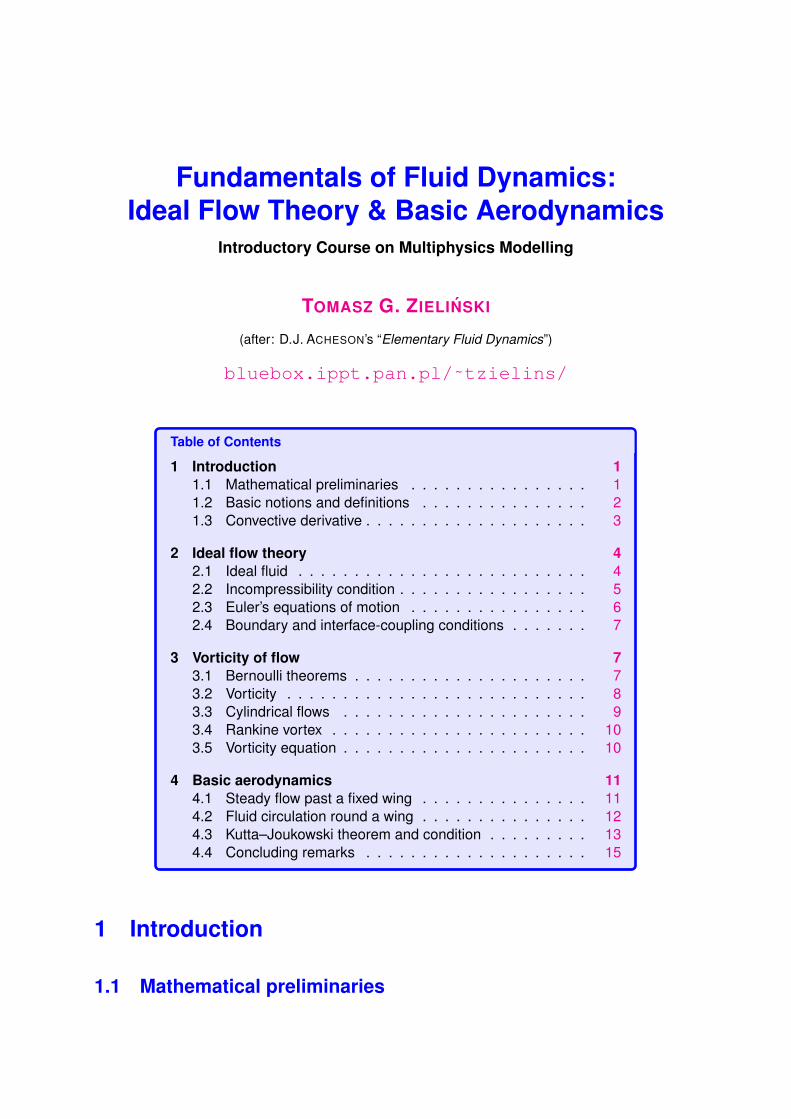
Theorem 1 (Divergence theorem). Let the region V be bounded by a simple sur-face S with unit outward normal n. Then:∫

S

f · n dS =

∫V

∇ · f dV ; in particular∫S

f n dS =

∫V

∇f dV . (1)

Theorem 2 (Stokes’ theorem). Let C be a simple closed curve spanned by a sur-face S with unit normal n. Then:

n

SC

∫C

f · dx =

∫S

(∇× f

)· n dS . (2)

Green’s theorem in the plane may be viewed as a special case of Stokes’ theorem(with f =

[u(x, y), v(x, y), 0

]):∫

C

u dx+ v dy =

∫S

(∂v

∂x− ∂u

∂y

)dx dy . (3)

1.2 Basic notions and definitions

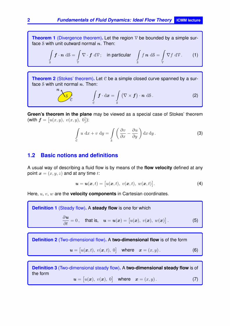
A usual way of describing a fluid flow is by means of the flow velocity defined at anypoint x = (x, y, z) and at any time t:

u = u(x, t) =[u(x, t), v(x, t), w(x, t)

]. (4)

Here, u, v, w are the velocity components in Cartesian coordinates.

Definition 1 (Steady flow). A steady flow is one for which

∂u

∂t= 0 , that is, u = u(x) =

[u(x), v(x), w(x)

]. (5)

Definition 2 (Two-dimensional flow). A two-dimensional flow is of the form

u =[u(x, t), v(x, t), 0

]where x = (x, y) . (6)

Definition 3 (Two-dimensional steady flow). A two-dimensional steady flow is ofthe form

u =[u(x), v(x), 0

]where x = (x, y) . (7)

ICMM lecture Fundamentals of Fluid Dynamics: Ideal Flow Theory 3

Definition 4 (Streamline). A streamline is a curve which, at any particular time t,has the same direction as u(x, t) at each point. A streamline x = x(s), y = y(s),z = z(s) (s is a parameter) is obtained by solving at a particular time t:

dxds

u=

dyds

v=

dzds

w. (8)

Remarks:

For a steady flow the streamline pattern is the same at all times, and fluid particlestravel along them.

In an unsteady flow, streamlines and particle paths are usually quite different.

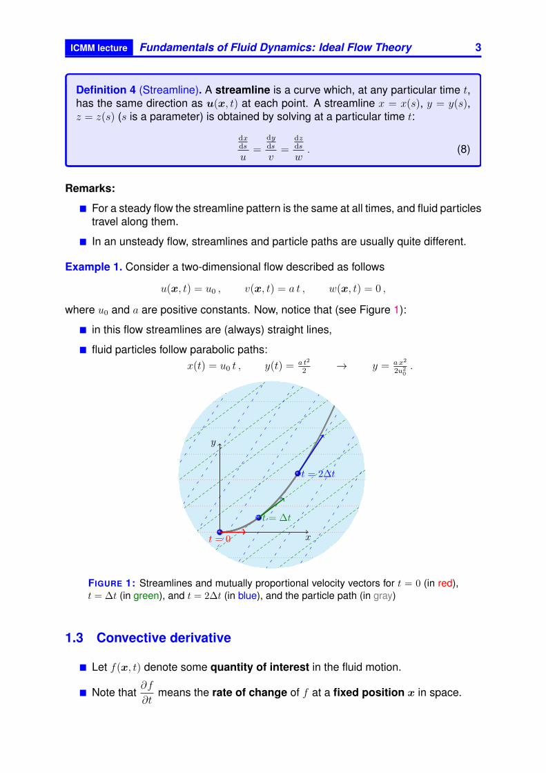
Example 1. Consider a two-dimensional flow described as follows

u(x, t) = u0 , v(x, t) = a t , w(x, t) = 0 ,

where u0 and a are positive constants. Now, notice that (see Figure 1):

in this flow streamlines are (always) straight lines,

fluid particles follow parabolic paths:x(t) = u0 t , y(t) = a t2

2→ y = a x2

2u20.

x

y

t = 0

t = ∆t

t = 2∆t

FIGURE 1: Streamlines and mutually proportional velocity vectors for t = 0 (in red),t = ∆t (in green), and t = 2∆t (in blue), and the particle path (in gray)

1.3 Convective derivative

Let f(x, t) denote some quantity of interest in the fluid motion.

Note that∂f

∂tmeans the rate of change of f at a fixed position x in space.


The rate of change of f “following the fluid” is

Df

Dt=

d

dtf(x(t), t

)=∂f

∂x

dx

dt+∂f

∂t(9)

where x(t) =[x(t), y(t), z(t)

]is understood to change with time at the local flow

velocity u, so thatdx

dt=

[dx

dt,

dy

dt,

dz

dt

]=[u, v, w

]. (10)

Therefore,

∂f

∂x

dx

dt=∂f

∂x

dx

dt+∂f

∂y

dy

dt+∂f

∂z

dz

dt=∂f

∂xu+

∂f

∂yv +

∂f

∂zw = (u · ∇)f . (11)

Definition 5 (Convective derivative). The convective derivative (a.k.a. the ma-terial, particle, Lagrangian, or total-time derivative) is a derivative taken withrespect to a coordinate system moving with velocity u (i.e., following the fluid):

Df

Dt=∂f

∂t+ (u · ∇)f . (12)

By applying the convective derivative to the velocity components u, v, w in turn itfollows that the acceleration of a fluid particle is

Du

Dt=∂u

∂t+ (u · ∇)u . (13)

Example 2. Consider fluid in uniform rotation with angular velocity Ω, so that:

u = −Ω y , v = Ωx , w = 0 .

The flow is steady so ∂u∂t

= 0, but

Du

Dt=

(− Ω y

∂

∂x+ Ωx

∂

∂y

)[− Ω y, Ωx, 0

]= −Ω2

[x, y, 0

].

represents the centrifugal acceleration Ω2√x2 + y2 towards the rotation axis.

2 Ideal flow theory

2.1 Ideal fluid

Definition 6 (Ideal fluid). Properties of an ideal fluid:

1. it is incompressible: no fluid element can change in volume as it moves;

2. it has constant density: % is the same for all fluid elements and for all time t(a consequence of incompressibility);


3. it is inviscid, so that the force exerted across a geometrical surface ele-ment n δS within the fluid is

pn δS ,

where p(x, t) is a scalar function of pressure, independent on the normal n.

Remarks:

All fluids are to some extent compressible and viscous.

Air, being highly compressible, can behave like an incompressible fluid if theflow speed is much smaller than the speed of sound.

2.2 Incompressibility condition

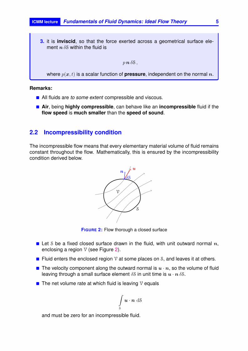
The incompressible flow means that every elementary material volume of fluid remainsconstant throughout the flow. Mathematically, this is ensured by the incompressibilitycondition derived below.

S

V

δS

nu

FIGURE 2: Flow thorough a closed surface

Let S be a fixed closed surface drawn in the fluid, with unit outward normal n,enclosing a region V (see Figure 2).

Fluid enters the enclosed region V at some places on S, and leaves it at others.

The velocity component along the outward normal is u · n, so the volume of fluidleaving through a small surface element δS in unit time is u · n δS.

The net volume rate at which fluid is leaving V equals

∫S

u · n dS

and must be zero for an incompressible fluid.


Now, using the divergence theorem and the assumption of the “smoothness” of flow(i.e., continuous velocity gradient) gives the condition for incompressible flow.

Incompressibility condition

For all regions within an incompressible fluid∫S

u · n dS =

∫V

∇ · u dV = 0 (14)

which (assuming that ∇·u is continuous) yields the following important constrainton the velocity field: ∇ · u = 0

(everywhere in the fluid).(15)

2.3 Euler’s equations of motion

The net force exerted on an arbitrary fluid element is

−∫S

pn dS = −∫V

∇p dV (16)

(the negative sign arises because n points out of S). Now, provided that ∇p is continu-ous it will be almost constant over a small element δV. The net force on such a smallelement due to the pressure of the surrounding fluid will therefore be

−∇p δV .

The principle of linear momentum implies that the following forces must be equalfor a fluid element of volume δV:

(− ∇p + % g

)δV – the total (external) net force acting on the element in

the presence of gravitational body force per unit mass g[

Nkg

= ms2

](the gravity

acceleration),

% δV DuDt

– the inertial force, that is, the product of the element’s mass (whichis conserved) and its acceleration.

This results in the Euler’s momentum equation for an ideal fluid. Another equation ofmotion is the incompressibility constraint (15).


Euler’s equations of motion for an ideal fluid

Du

Dt= −1

%∇p+ g , ∇ · u = 0 . (17)

2.4 Boundary and interface-coupling conditions

Impermeable surface. The fluid cannot flow through the boundary which means thatthe normal velocity is constrained (no-penetration condition):

u · n = un . (18)

Here, un is the prescribed normal velocity of the impermeable boundary (un = 0for motionless, rigid boundary).

Free surface. Pressure condition (involving surface tension effects):

p = p0 ± 2T κmean . (19)

Here: p0 is the ambient pressure,T is the surface tension,κmean is the local mean curvature of the free surface.

Fluid interface. The continuity of normal velocity and pressure at the interface be-tween fluids 1 and 2:(

u(1) − u(2))· n = 0 , p(1) − p(2) = 0± 2

(T (1) + T (2)

)κmean . (20)

3 Vorticity of flow

3.1 Bernoulli theorems

The gravitational force, being conservative, can be written as the gradient of apotential:

g = −∇χ where χ = g z[

m2

s2

], (21)

and the momentum equation

∂u

∂t+ (u · ∇)u︸︷︷︸(∇×u)×u+∇( 1

2u2)

= −∇(p

%+ χ

)(22)

can be cast into the following form


∂u

∂t+ (∇× u)× u = −∇H where H =

p

%+

1

2u2 + χ . (23)

For a steady flow (∂u∂t

= 0): (∇× u)× u = −∇H u·−→ (u · ∇)H = 0 .

Theorem 3 (Bernoulli streamline theorem). If an ideal fluid is in steady flow, thenH is constant along a streamline.

Definition 7 (Irrotational flow). A flow is irrotational if ∇× u = 0.

For a steady irrotational flow: ∇H = 0 .

Theorem 4 (Bernoulli theorem for irrotational flow). If an ideal fluid is in steadyirrotational flow, then H is constant throughout the whole fluid.

3.2 Vorticity

Definition 8 (Vorticity). Vorticity is a concept of central importance in fluid dynam-ics; it is defined as

ω = ∇×u[

1s

]. (24)

Remarks:

For an irrotational flow: ω = 0.

Vorticity has nothing directly to do with any global rotation of the fluid.

Interpretation of vorticity (in 2D)

For two-dimensional flow (when u =[u(x, t), v(x, t), 0

]):

ω =[0, 0, ω

]where ω =

∂v

∂x− ∂u

∂y. (25)

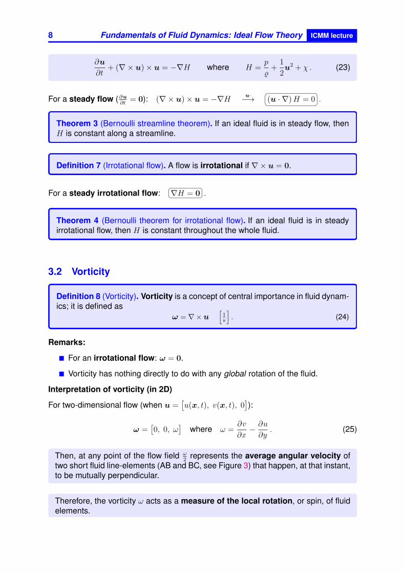
Then, at any point of the flow field ω2

represents the average angular velocity oftwo short fluid line-elements (AB and BC, see Figure 3) that happen, at that instant,to be mutually perpendicular.

Therefore, the vorticity ω acts as a measure of the local rotation, or spin, of fluidelements.


A B

C

δx

δy

∂u

∂xδx

∂v

∂xδx

∂u

∂yδy

∂v

∂yδy

average angular velocity:ωAB + ωAC

2=

1

2

( ∂v∂x− ∂u

∂y

)=ω

2

FIGURE 3: Interpretation of vorticity in 2D flow. The velocity components are relativeto the fluid particle at A.

3.3 Cylindrical flows

Flow may be written in cylindrical polar coordinates (r, θ, z):

u = ur er + uθ eθ + uz ez . (26)

Consider the following steady, two-dimensional flows with uθ = uθ(r) and ur = uz = 0(here, Ω [1/s] and a [m] are constants):

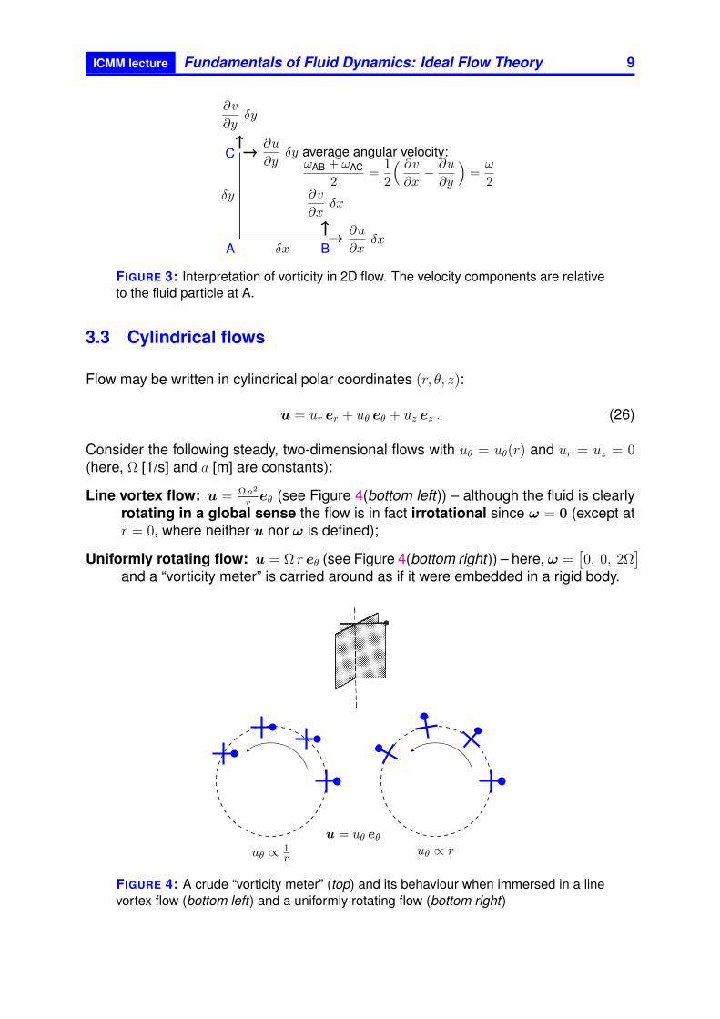
Line vortex flow: u = Ω a2

reθ (see Figure 4(bottom left)) – although the fluid is clearly

rotating in a global sense the flow is in fact irrotational since ω = 0 (except atr = 0, where neither u nor ω is defined);

Uniformly rotating flow: u = Ω r eθ (see Figure 4(bottom right)) – here, ω =[0, 0, 2Ω

]and a “vorticity meter” is carried around as if it were embedded in a rigid body.

u = uθ eθuθ ∝ 1

ruθ ∝ r

FIGURE 4: A crude “vorticity meter” (top) and its behaviour when immersed in a linevortex flow (bottom left) and a uniformly rotating flow (bottom right)


3.4 Rankine vortex

Definition 9 (Rankine vortex). Rankine vortex is a steady, two-dimensional flowdescribed as

u = uθ eθ with uθ =

Ω r for r ≤ a (uniformly rotating flow),Ω a2

rfor r > a (line vortex flow),

(27)

where Ω and a are constants. Therefore,

ω = ω ez with ω =1

r

∂(r uθ)

∂r

1r∂(Ω r2)∂r

= 2 Ω for r ≤ a (vortex core),1r∂(Ω a2)∂r

= 0 for r > a (irrotational).(28)

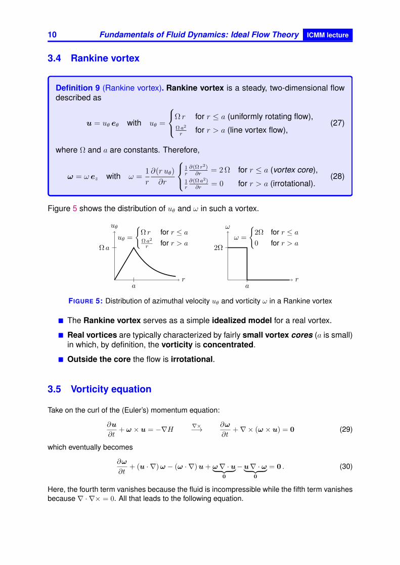
Figure 5 shows the distribution of uθ and ω in such a vortex.

r

uθ

Ω a

a

uθ =

Ω r for r ≤ aΩ a2

r for r > a

r

ω

2Ω

a

ω =

2Ω for r ≤ a0 for r > a

FIGURE 5: Distribution of azimuthal velocity uθ and vorticity ω in a Rankine vortex

The Rankine vortex serves as a simple idealized model for a real vortex.

Real vortices are typically characterized by fairly small vortex cores (a is small)in which, by definition, the vorticity is concentrated.

Outside the core the flow is irrotational.

3.5 Vorticity equation

Take on the curl of the (Euler’s) momentum equation:

∂u

∂t+ ω × u = −∇H ∇×−→ ∂ω

∂t+∇× (ω × u) = 0 (29)

which eventually becomes

∂ω

∂t+ (u · ∇)ω − (ω · ∇)u + ω∇ · u︸︷︷︸

0

−u∇ · ω︸︷︷︸0

= 0 . (30)

Here, the fourth term vanishes because the fluid is incompressible while the fifth term vanishesbecause ∇ · ∇× = 0. All that leads to the following equation.


Vorticity equation

∂ω

∂t+ (u · ∇)ω = (ω · ∇)u , or

Dω

Dt= (ω · ∇)u . (31)

The vorticity equation is extremely valuable: as a matter of fact, it involves only u sincethe pressure has been eliminated and ω = ∇× u.

In the two-dimensional flow (u =[u(x, t), v(x, t), 0

], ω =

[0, 0, ω(x, t)

]) of an ideal fluid

subject to a conservative body force g the vorticity ω of each individual fluid element isconserved:

Dω

Dt= 0 . (32)

In the steady, two-dimensional flow of an ideal fluid subject to a conservative body force gthe vorticity ω is constant along a streamline:

(u · ∇)ω = 0 . (33)

4 Basic aerodynamics

4.1 Steady flow past a fixed wing

Steady flow past a wing at small angle of attack (incidence) is typically irrota-tional. This results from equation (33) and Figure 6 as discussed below.

FIGURE 6: Irrotational flow past a fixed wing at small angle of attack.

There are no regions of closed streamlines in the flow (Figure 6); all thestreamlines can be traced back to x→ −∞.

The vorticity is constant along each streamline, cf. Equation (33), and henceequal on each one to whatever it is on that particular streamline at x→ −∞.

As the flow is uniform at x → −∞, the vorticity is zero on all streamlines there;hence, it is zero throughout the flow field around the wing.

Figure 7 shows typical measured pressure distribution on the upper and lower surfacesof a fixed wing in steady flow. One should notice what follows:


FIGURE 7: Typical pressure distribution on a wing in steady flow

the pressures on the upper surface are substantially lower than the free-streamvalue p∞;

the pressures on the lower surface are a little higher than p∞;

in fact, the wing gets most of its lift from a suction effect on its upper surface.

Why the pressures above the wing are less than those below?

The flow is irrotational and the Bernoulli theorem states that %H = p + 12%u

2 isconstant throughout 2D irrotational flows.

Explaining the pressure differences, and hence the lift on the wing, thus reduces toexplaining why the flow speeds above the wing are greater than those below.

An explanation is in terms of the concept of circulation.

4.2 Fluid circulation round a wing

Definition 10 (Circulation). The circulation Γ round some closed curve C lying inthe fluid region is defined as

Γ =

∫C

u · dx[

m2

s

]. (34)

If S is the region enclosed by the curve C then the Stokes’ theorem gives

Γ =

∫C

u · dx =

∫S

(∇× u) · n dS , (35)


or in the two-dimensional context

Γ =

∫C

u dx+ v dy =

∫S

(∂v

∂x− ∂u

∂y

)dx dy . (36)

Notice that in the surface integrals vorticity terms appear.

Corollaries. The following statements can be formulated about the fluid circulationround a wing:

Γ = 0 if the closed curve C is spanned by a surface S which lies wholly in theregion of irrotational flow, that is, Γ = 0 for any closed curve not enclosing thewing.

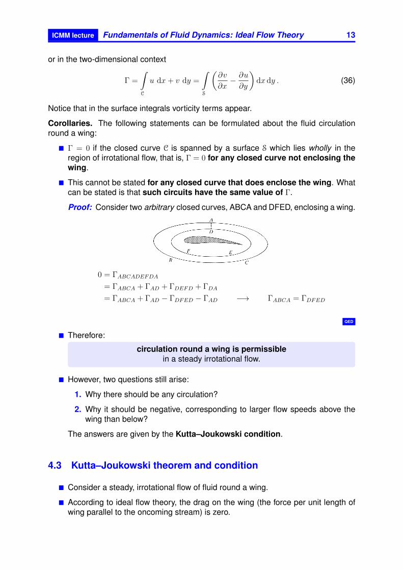
This cannot be stated for any closed curve that does enclose the wing. Whatcan be stated is that such circuits have the same value of Γ.

Proof: Consider two arbitrary closed curves, ABCA and DFED, enclosing a wing.

0 = ΓABCADEFDA

= ΓABCA + ΓAD + ΓDEFD + ΓDA

= ΓABCA + ΓAD − ΓDFED − ΓAD −→ ΓABCA = ΓDFED

QED

Therefore:

circulation round a wing is permissiblein a steady irrotational flow.

However, two questions still arise:

1. Why there should be any circulation?

2. Why it should be negative, corresponding to larger flow speeds above thewing than below?

The answers are given by the Kutta–Joukowski condition.

4.3 Kutta–Joukowski theorem and condition

Consider a steady, irrotational flow of fluid round a wing.

According to ideal flow theory, the drag on the wing (the force per unit length ofwing parallel to the oncoming stream) is zero.


What is the lift of the wing (i.e., the force per unit length of wing perpendicular tothe stream) is stated by the following theorem.

Theorem 5 (Kutta–Joukowski lift theorem). Let % be the fluid density and U theflow speed at infinity. Then, the lift of the wing is

Fy = −%U Γ[

Nm

], (37)

where Γ is the fluid circulation around the wing.

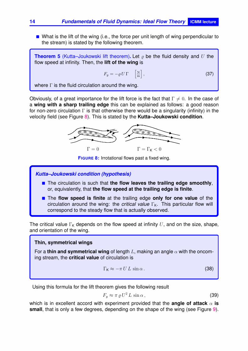
Obviously, of a great importance for the lift force is the fact that Γ 6= 0. In the case ofa wing with a sharp trailing edge this can be explained as follows: a good reasonfor non-zero circulation Γ is that otherwise there would be a singularity (infinity) in thevelocity field (see Figure 8). This is stated by the Kutta–Joukowski condition.

Γ = 0 Γ = ΓK < 0

FIGURE 8: Irrotational flows past a fixed wing.

Kutta–Joukowski condition (hypothesis)

The circulation is such that the flow leaves the trailing edge smoothly,or, equivalently, that the flow speed at the trailing edge is finite.

The flow speed is finite at the trailing edge only for one value of thecirculation around the wing: the critical value ΓK. This particular flow willcorrespond to the steady flow that is actually observed.

The critical value ΓK depends on the flow speed at infinity U , and on the size, shape,and orientation of the wing.

Thin, symmetrical wings

For a thin and symmetrical wing of length L, making an angle α with the oncom-ing stream, the critical value of circulation is

ΓK ≈ −π U L sinα . (38)

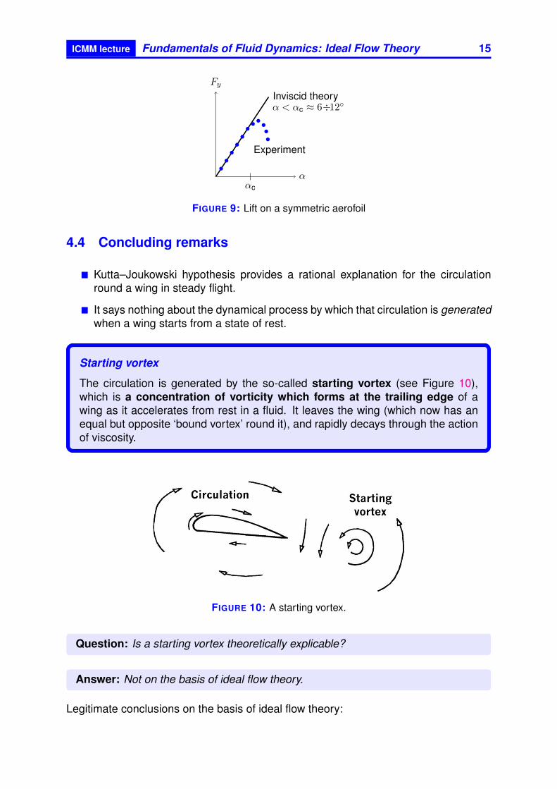
Using this formula for the lift theorem gives the following result

Fy ≈ π %U2 L sinα , (39)

which is in excellent accord with experiment provided that the angle of attack α issmall, that is only a few degrees, depending on the shape of the wing (see Figure 9).


Fy

ααc

Inviscid theoryα < αc ≈ 6÷12

Experiment

FIGURE 9: Lift on a symmetric aerofoil

4.4 Concluding remarks

Kutta–Joukowski hypothesis provides a rational explanation for the circulationround a wing in steady flight.

It says nothing about the dynamical process by which that circulation is generatedwhen a wing starts from a state of rest.

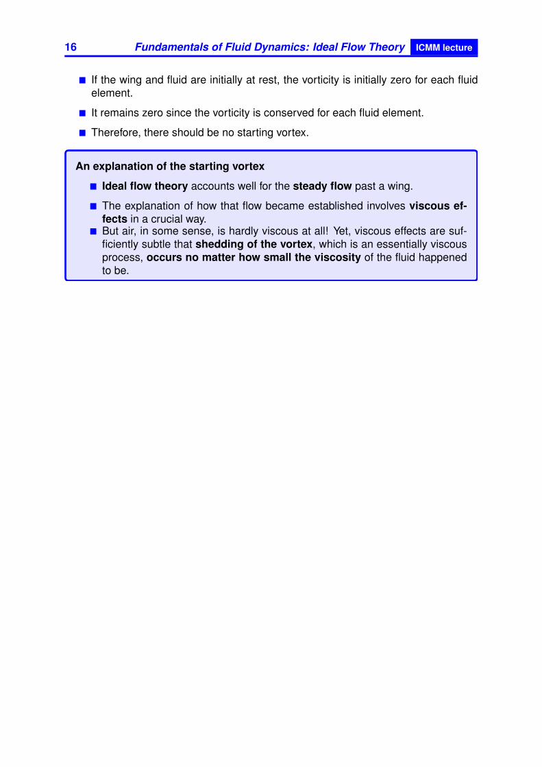
Starting vortex

The circulation is generated by the so-called starting vortex (see Figure 10),which is a concentration of vorticity which forms at the trailing edge of awing as it accelerates from rest in a fluid. It leaves the wing (which now has anequal but opposite ‘bound vortex’ round it), and rapidly decays through the actionof viscosity.

FIGURE 10: A starting vortex.

Question: Is a starting vortex theoretically explicable?

Answer: Not on the basis of ideal flow theory.

Legitimate conclusions on the basis of ideal flow theory:


If the wing and fluid are initially at rest, the vorticity is initially zero for each fluidelement.

It remains zero since the vorticity is conserved for each fluid element.

Therefore, there should be no starting vortex.

An explanation of the starting vortex

Ideal flow theory accounts well for the steady flow past a wing.

The explanation of how that flow became established involves viscous ef-fects in a crucial way.

But air, in some sense, is hardly viscous at all! Yet, viscous effects are suf-ficiently subtle that shedding of the vortex, which is an essentially viscousprocess, occurs no matter how small the viscosity of the fluid happenedto be.

Documents

(ICMM Lecture) Fundamentals of Fluid Dynamics: …bluebox.ippt.pan.pl/~tzielins/doc/ICMM_TGZielinski_IdealFlow.Notes.pdfFundamentals of Fluid Dynamics: Ideal Flow Theory & Basic Aerodynamics