Embed Size (px)
Citation preview
ICS-271:Notes 5: 1
Lecture 5: Constraint Satisfaction Problems
ICS 271 Fall 2008

ICS-271:Notes 5: 2
Outline
• The constraint network model
– Variables, domains, constraints, constraint graph, solutions
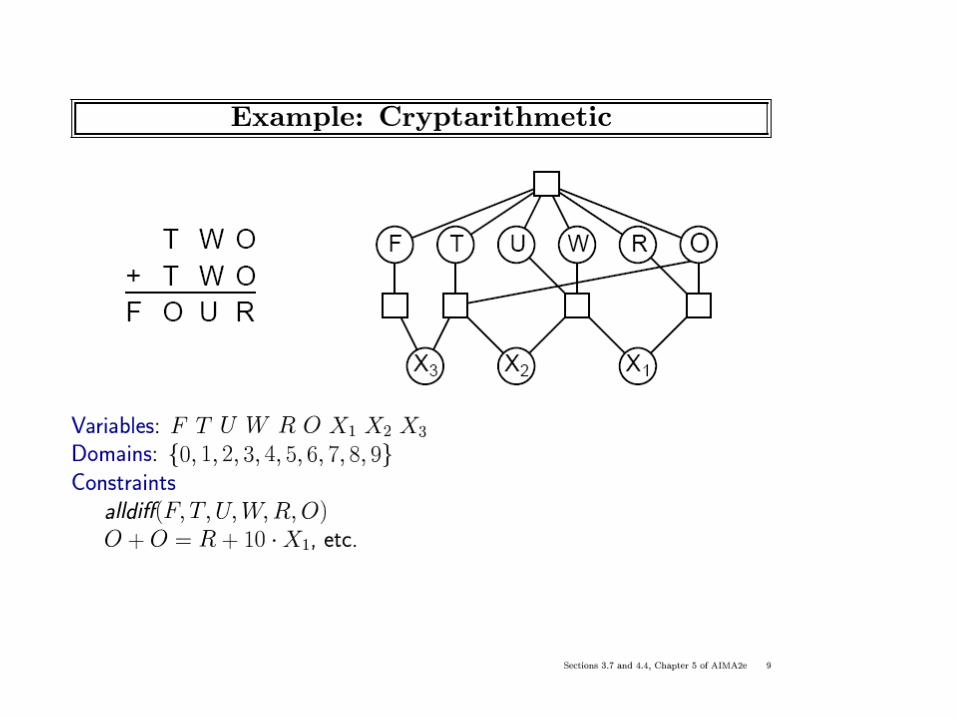
• Examples:
– graph-coloring, 8-queen, cryptarithmetic, crossword puzzles, vision problems,scheduling, design
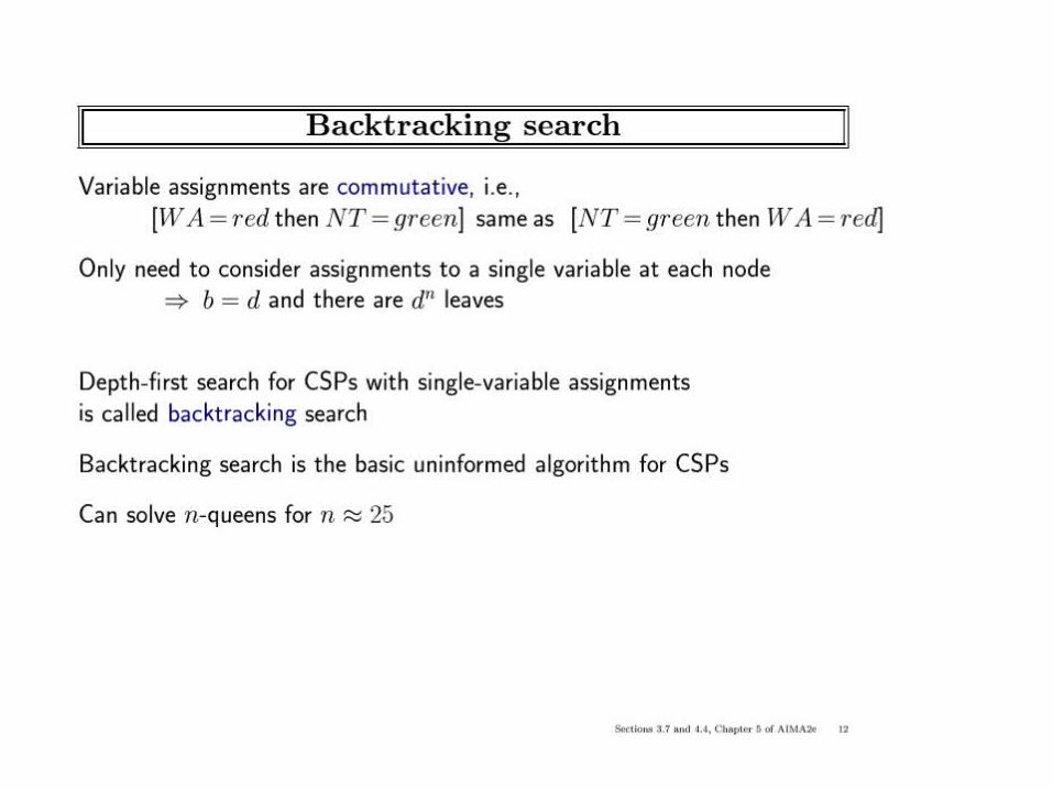
• The search space and naive backtracking,
• The constraint graph
• Consistency enforcing algorithms
– arc-consistency, AC-1,AC-3
• Backtracking strategies
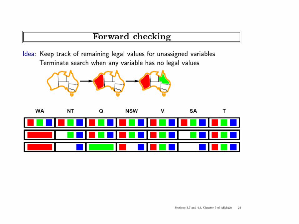
– Forward-checking, dynamic variable orderings
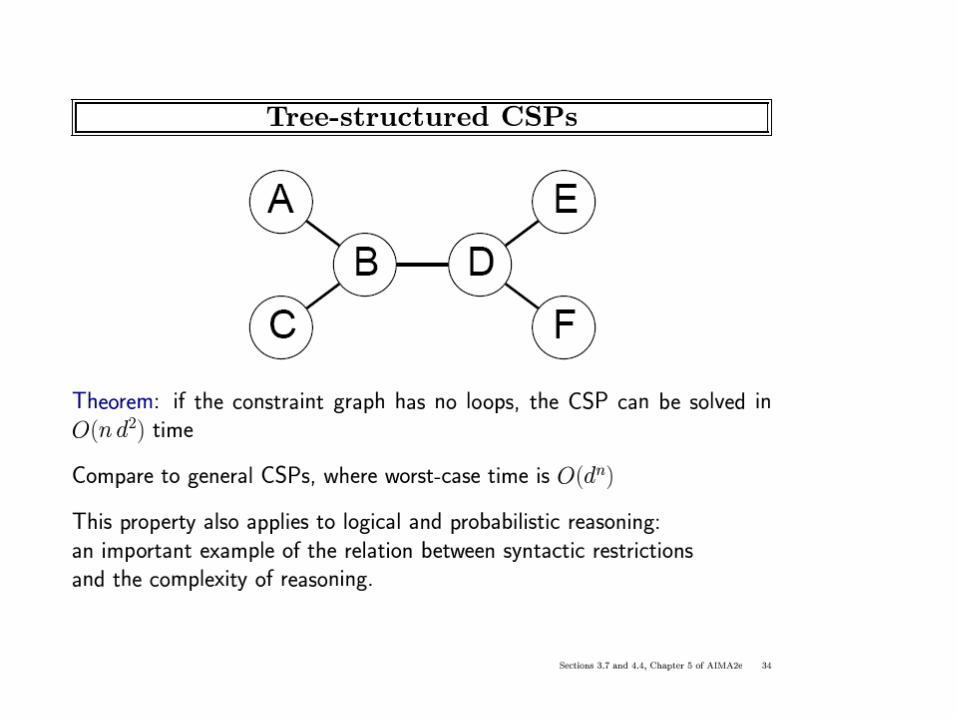
• Special case: solving tree problems
• Local search for CSPs

ICS-271:Notes 5: 3
ICS-271:Notes 5: 4
A Bred greenred yellowgreen redgreen yellowyellow greenyellow red
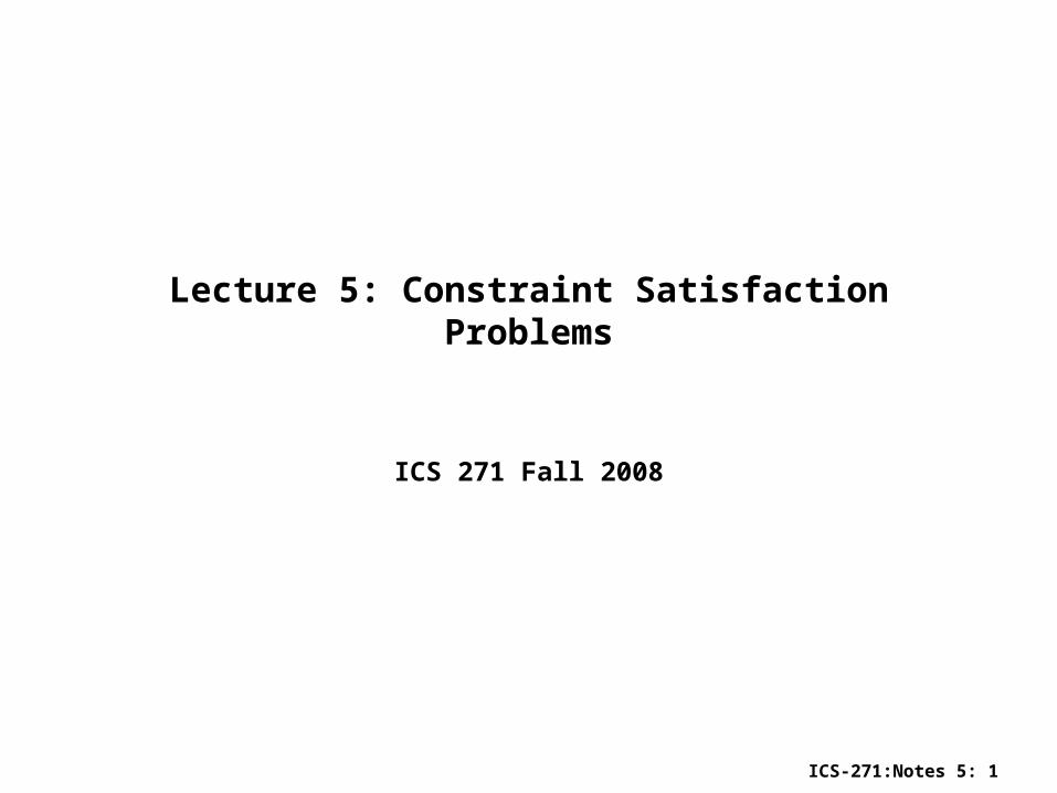
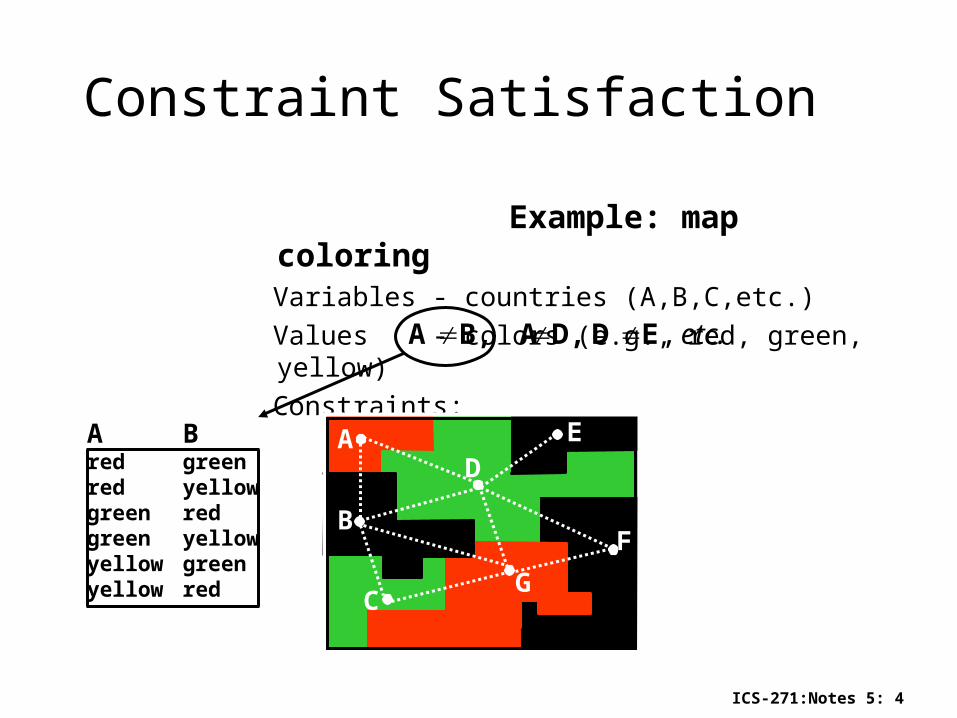
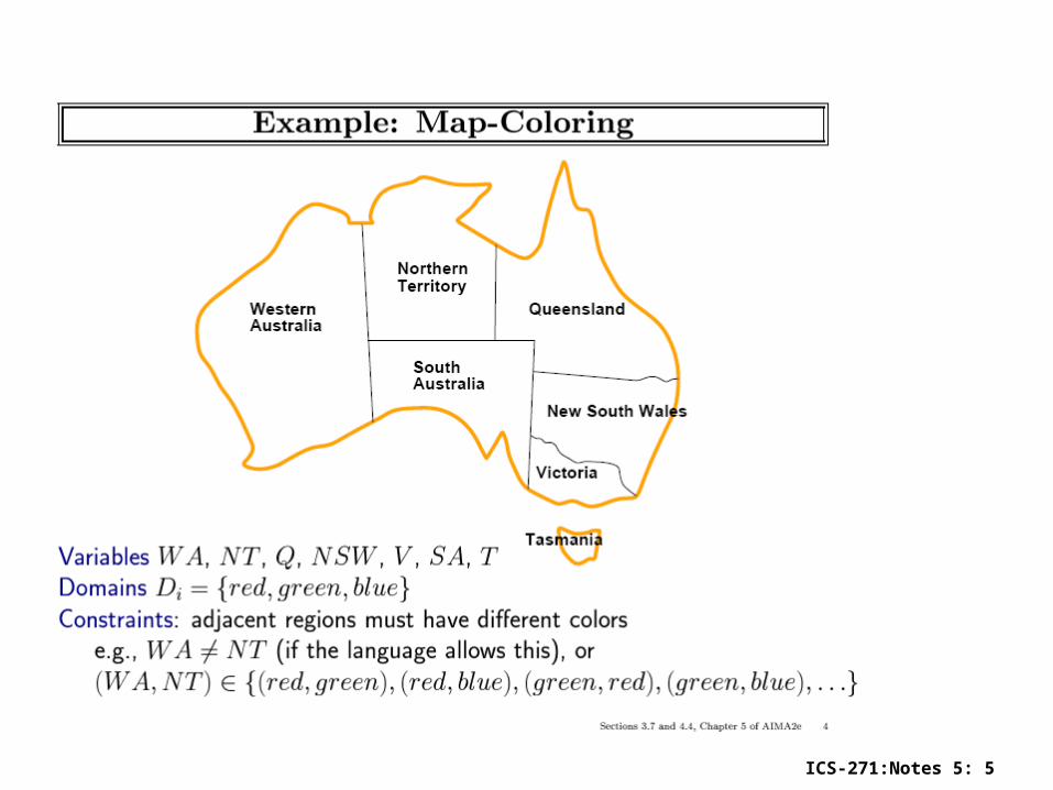
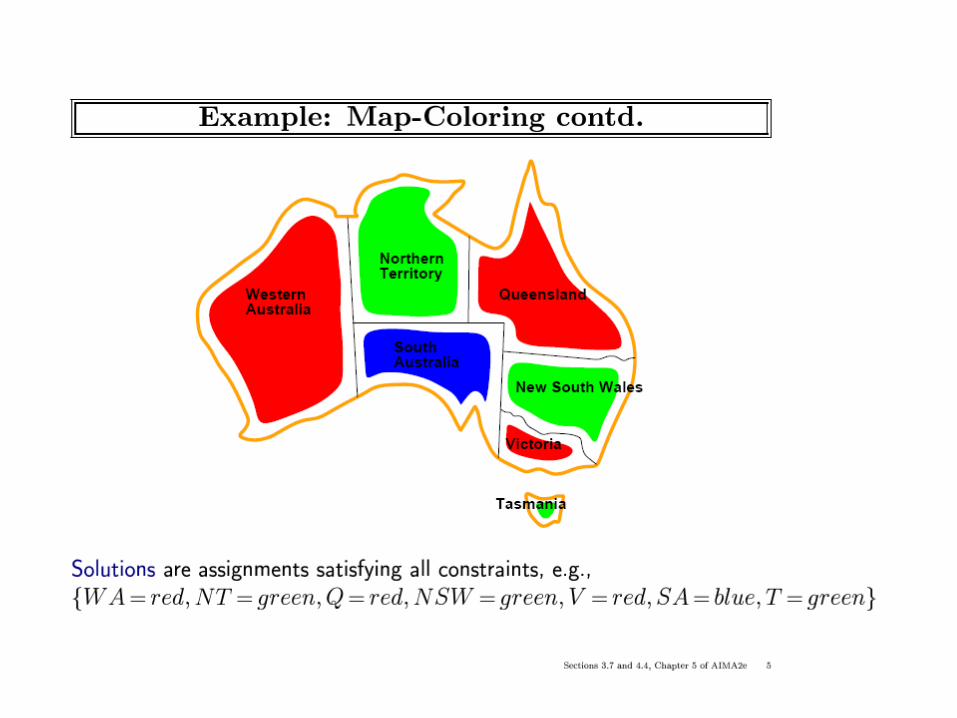
Constraint Satisfaction
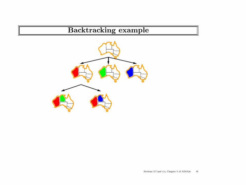
Example: map coloring Variables - countries (A,B,C,etc.)
Values - colors (e.g., red, green, yellow)
Constraints: etc. ,ED D, AB,A
C
A
B
DE
F
G
ICS-271:Notes 5: 5
ICS-271:Notes 5: 6
ICS-271:Notes 5: 7

ICS-271:Notes 5: 8
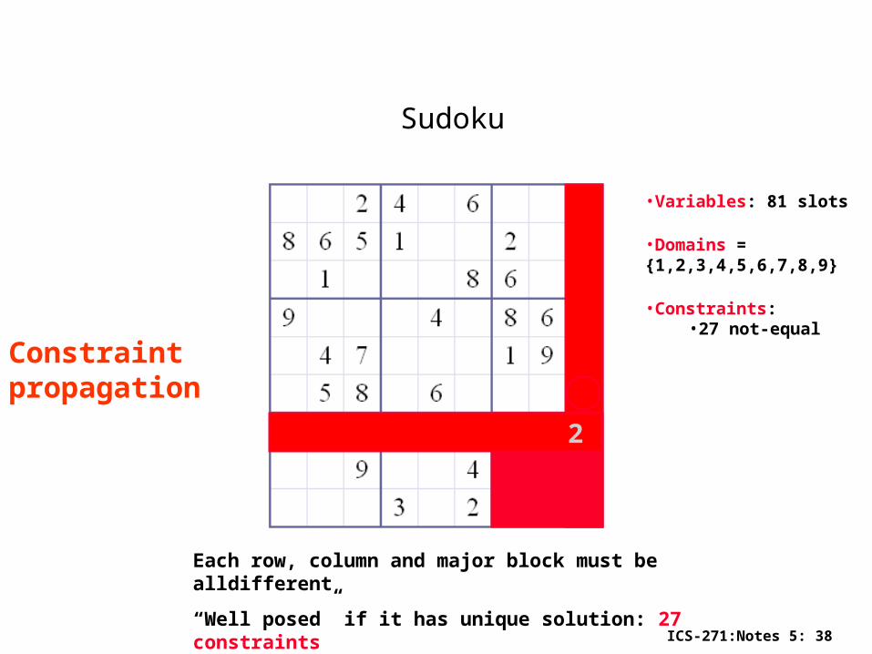
Sudoku
Each row, column and major block must be alldifferent
“Well posed” if it has unique solution: 27 constraints
2 34 62
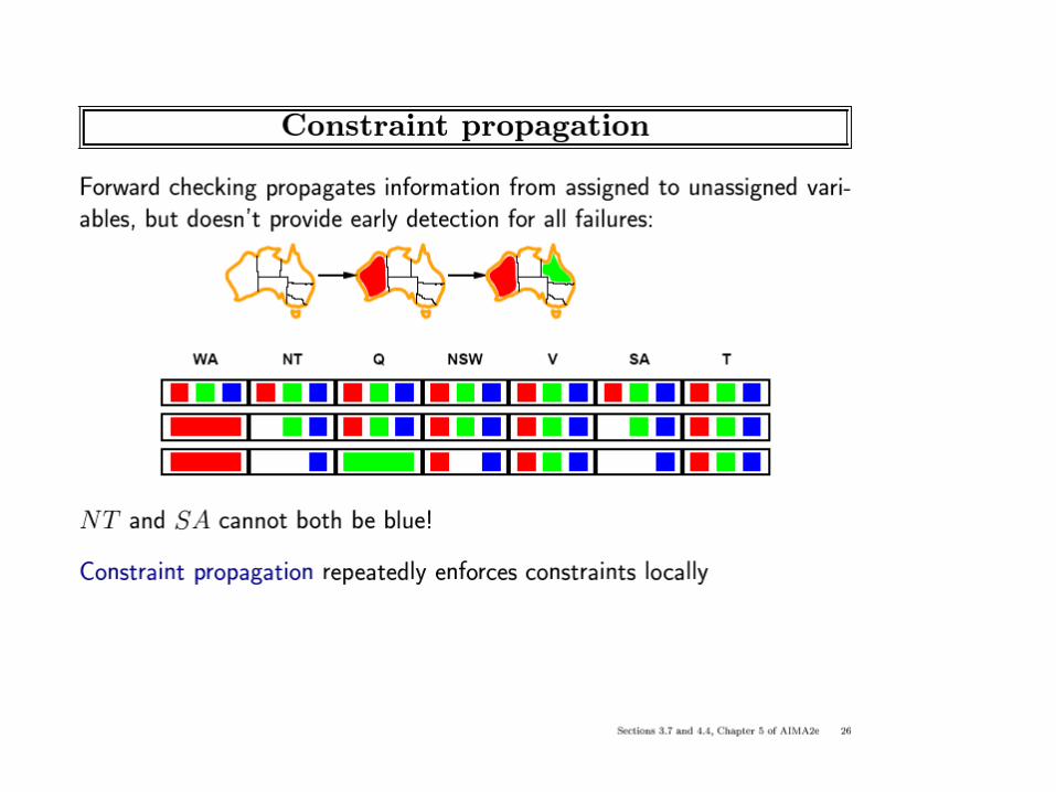
Constraint propagation
•Variables: 81 slots
•Domains = {1,2,3,4,5,6,7,8,9}
•Constraints: •27 not-equal
ICS-271:Notes 5: 9

ICS-271:Notes 5: 10
Varieties of constraints
• Unary constraints involve a single variable, – e.g., SA ≠ green
• Binary constraints involve pairs of variables,– e.g., SA ≠ WA
• Higher-order constraints involve 3 or more variables,– e.g., cryptarithmetic column constraints
–
–
–
ICS-271:Notes 5: 11
ICS-271:Notes 5: 13

ICS-271:Notes 5: 14
A network of binary constraints
• Variables
–
• Domains
– of discrete values:
• Binary constraints:
– which represent the list of allowed pairs of values, Rij is a subset of the Cartesian product: .
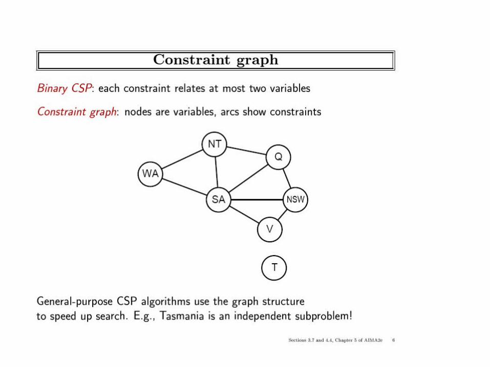
• Constraint graph:
– A node for each variable and an arc for each constraint
• Solution:
– An assignment of a value from its domain to each variable such that no constraint is violated.
• A network of constraints represents the relation of all solutions.
n,....,XX1
n,....,DD1
ji ,....,DDijR
},,),(|){( 1 jjiiijjin DXDxRxx,....,XXsol
1X
5X
4X 3X
2X
ICS-271:Notes 5: 15
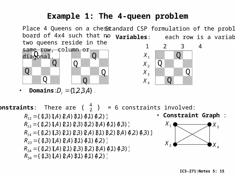
Example 1: The 4-queen problem
Q
Q QQ
Place 4 Queens on a chess board of 4x4 such that no two queens reside in the same row, column or diagonal.
Standard CSP formulation of the problem:• Variables: each row is a variable.
1X
4X3X2X
1 2 3 4
• Domains: }.4,3,2,1{iD
• Constraints: There are = 6 constraints involved:42( )
)}2,4)(1,4)(1,3)(4,2)(4,1)(3,1{(12 R)}3,4)(1,4)(4,3)(2,3)(3,2)(1,2)(4,1)(2,1{(13 R
)}3,4)(2,4)(4,3)(2,3)(1,3)(4,2)(3,2)(1,2)(3,1)(2,1{(14 R)}2,4)(1,4)(1,3)(4,2)(4,1)(3,1{(23 R
)}3,4)(1,4)(4,3)(2,3)(3,2)(1,2)(4,1)(2,1{(24 R)}2,4)(1,4)(1,3)(4,2)(4,1)(3,1{(34 R
• Constraint Graph :
1X
2X 4X
3X

ICS-271:Notes 5: 16
ICS-271:Notes 5: 17
ICS-271:Notes 5: 18
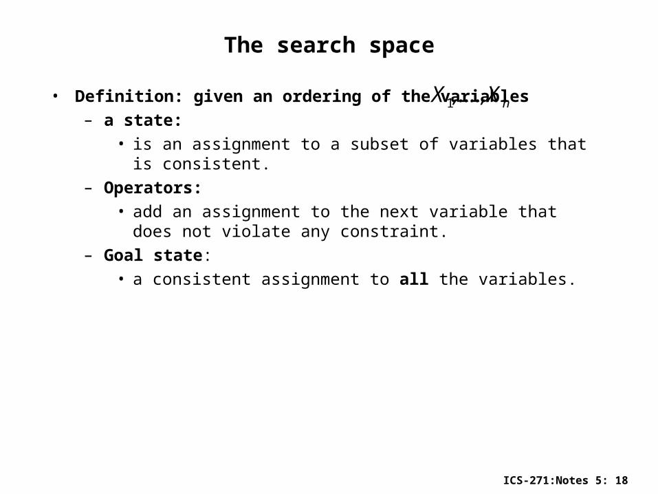
The search space
• Definition: given an ordering of the variables
– a state:
• is an assignment to a subset of variables that is consistent.
– Operators:
• add an assignment to the next variable that does not violate any constraint.
– Goal state:
• a consistent assignment to all the variables.
n,....,XX1
ICS-271:Notes 5: 19

ICS-271:Notes 5: 20
ICS-271:Notes 5: 21

ICS-271:Notes 5: 22

ICS-271:Notes 5: 23
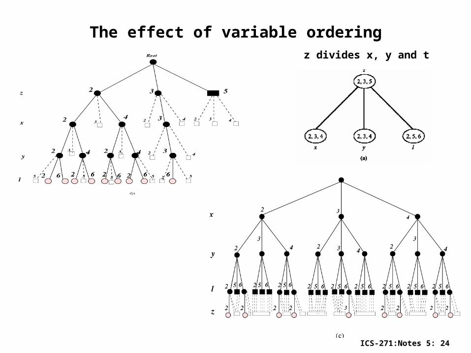
The search space depends on the variable orderings
ICS-271:Notes 5: 24
The effect of variable orderingz divides x, y and t

ICS-271:Notes 5: 25
Backtracking
• Complexity of extending a partial solution:– Complexity of consistent: O(e log t), t bounds #tuples, e bounds #constraints– Complexity of selectvalue: O(e k log t), k bounds domain size

ICS-271:Notes 5: 26
A coloring problem
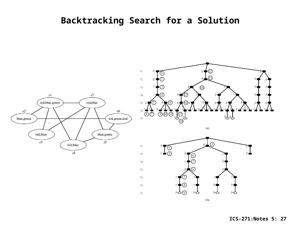
ICS-271:Notes 5: 27
Backtracking Search for a Solution
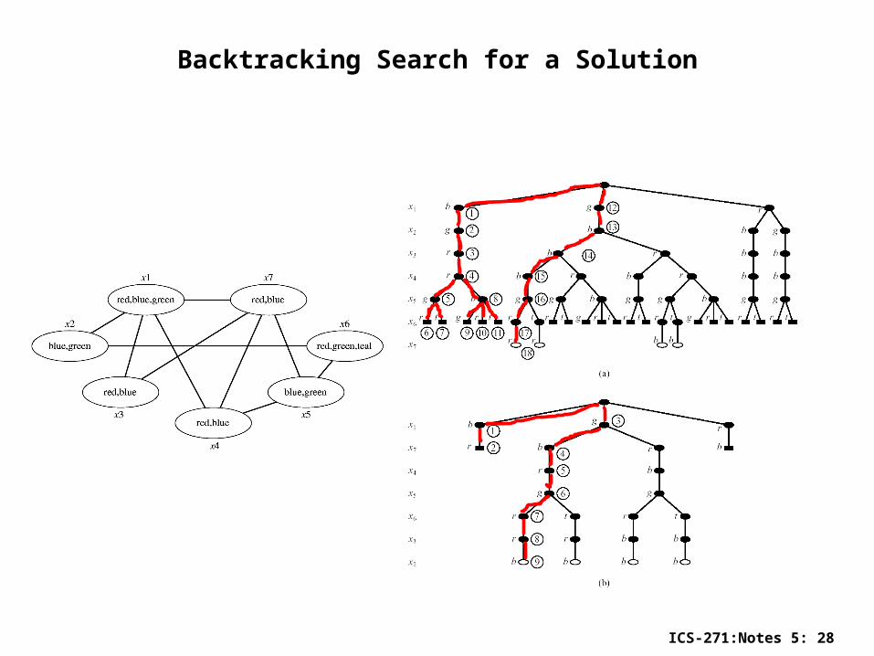
ICS-271:Notes 5: 28
Backtracking Search for a Solution

ICS-271:Notes 5: 29
Backtracking Search for All Solutions
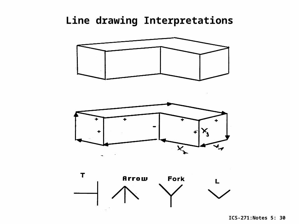
ICS-271:Notes 5: 30
Line drawing Interpretations

ICS-271:Notes 5: 31
Class scheduling/Timetabling
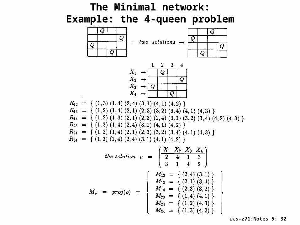
ICS-271:Notes 5: 32
The Minimal network:Example: the 4-queen problem
ICS-271:Notes 5: 33
Approximation algorithms
• Arc-consistency (Waltz, 1972)
• Path-consistency (Montanari 1974, Mackworth 1977)
• I-consistency (Freuder 1982)
• Transform the network into smaller and smaller networks.
ICS-271:Notes 5: 34
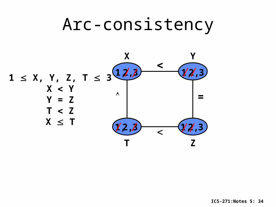
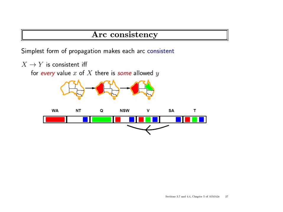
Arc-consistency
32,1,
32,1, 32,1,
1 X, Y, Z, T 3X YY = ZT ZX T
X Y
T Z
32,1,
=

ICS-271:Notes 5: 35
1 X, Y, Z, T 3X YY = ZT ZX T
X Y
T Z
=
1 3
2 3
• Incorporated into backtracking search
• Constraint programming languages powerful approach for modeling and solving combinatorial optimization problems.
Arc-consistency
ICS-271:Notes 5: 36
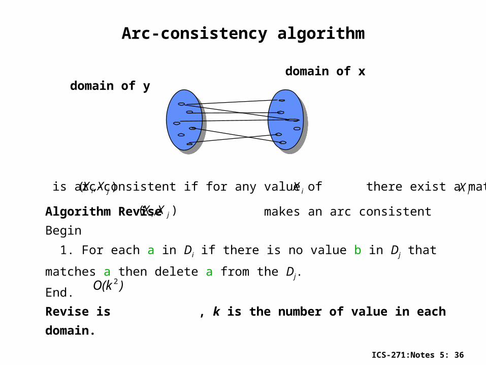
Arc-consistency algorithm
domain of x domain of y
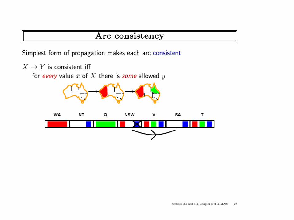
Arc is arc-consistent if for any value of there exist a matching value of
Algorithm Revise makes an arc consistent
Begin
1. For each a in Di if there is no value b in Dj that matches a then delete a from the Dj.
End.
Revise is , k is the number of value in each domain.
)( ji ,XX iX iX
)( ji ,XX
)O(k 2
ICS-271:Notes 5: 37
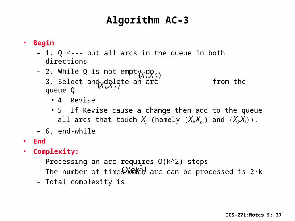
Algorithm AC-3
• Begin
– 1. Q <--- put all arcs in the queue in both directions
– 2. While Q is not empty do,
– 3. Select and delete an arc from the queue Q
• 4. Revise
• 5. If Revise cause a change then add to the queue all arcs that touch Xi (namely (Xi,Xm) and (Xl,Xi)).
– 6. end-while
• End
• Complexity:
– Processing an arc requires O(k^2) steps
– The number of times each arc can be processed is 2·k
– Total complexity is
)( ji ,XX
)( ji ,XX
)O(ek 3
ICS-271:Notes 5: 38
Sudoku
Each row, column and major block must be alldifferent
“Well posed” if it has unique solution: 27 constraints
2 34 62
Constraint propagation
•Variables: 81 slots
•Domains = {1,2,3,4,5,6,7,8,9}
•Constraints: •27 not-equal
ICS-271:Notes 5: 39
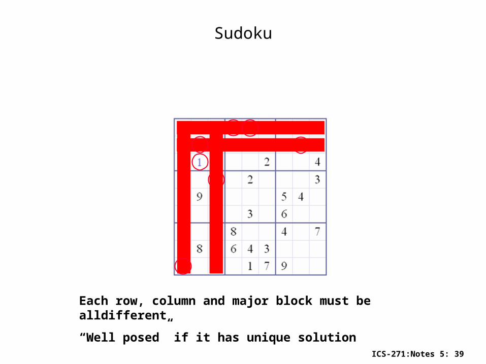
Sudoku
Each row, column and major block must be alldifferent
“Well posed” if it has unique solution
ICS-271:Notes 5: 40
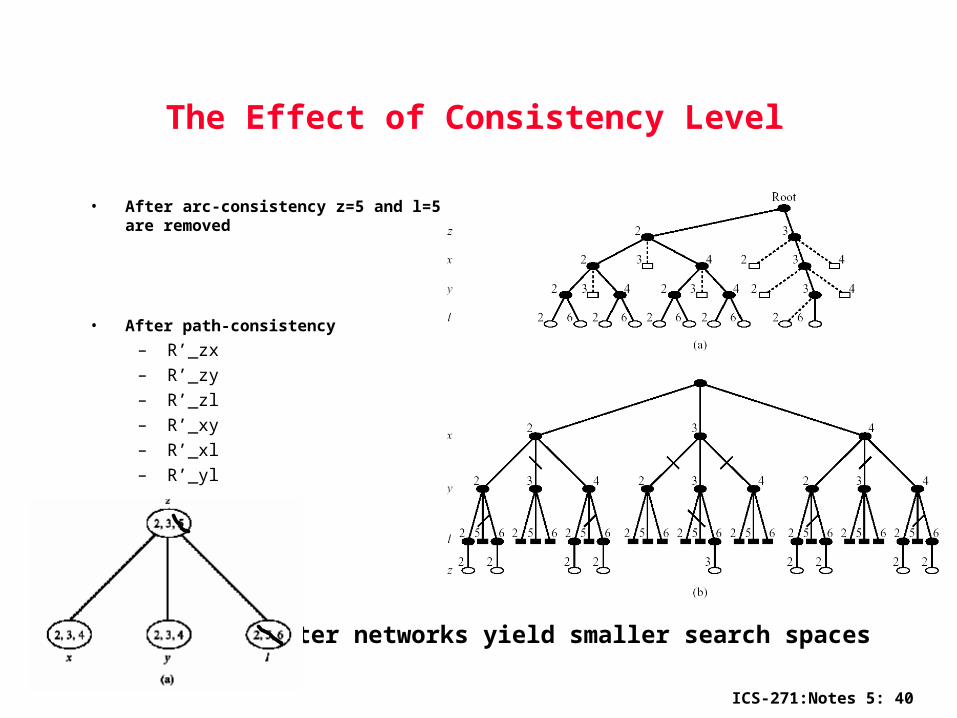
The Effect of Consistency Level
• After arc-consistency z=5 and l=5 are removed
• After path-consistency
– R’_zx– R’_zy– R’_zl– R’_xy– R’_xl– R’_yl
Tighter networks yield smaller search spaces

ICS-271:Notes 5: 41
• Before search: (reducing the search space)– Arc-consistency, path-consistency, i-consistency– Variable ordering (fixed)
• During search:– Look-ahead schemes:
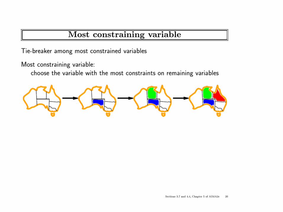
• Value ordering/pruning (choose a least restricting value), • Variable ordering (Choose the most constraining variable)
– Look-back schemes:• Backjumping• Constraint recording• Dependency-directed backtracking
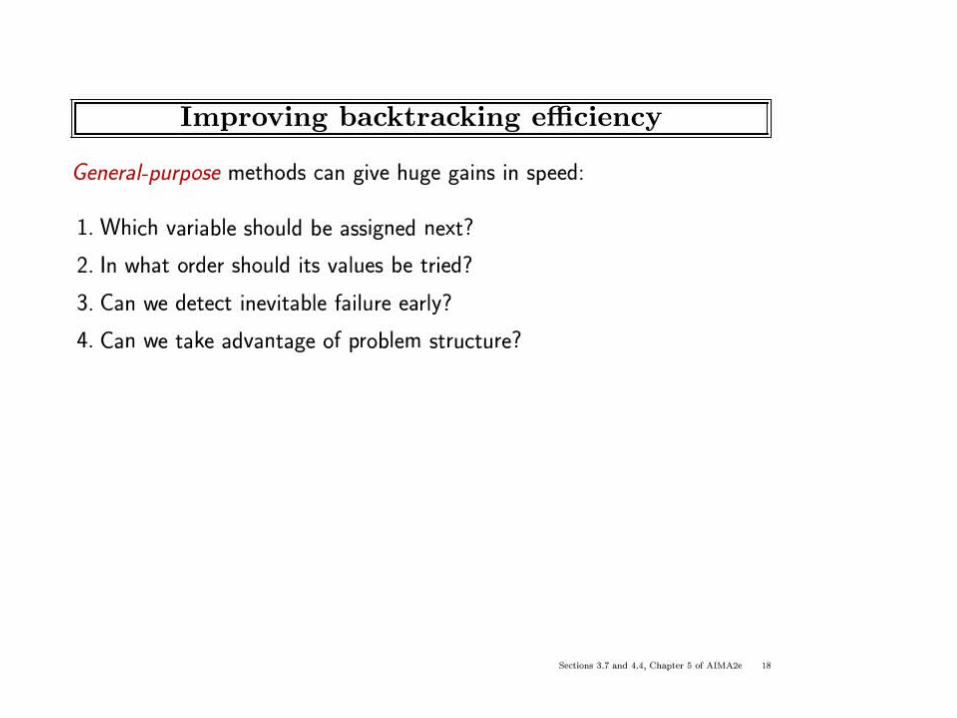
Improving Backtracking O(exp(n))
ICS-271:Notes 5: 42
ICS-271:Notes 5: 43
Look-ahead: Variable and value orderings
• Intuition: – Choose value least likely to yield a dead-end– Choose a variable that will detect failures early– Approach: apply propagation at each node in the search tree
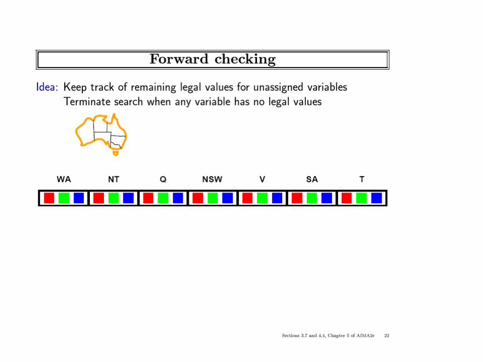
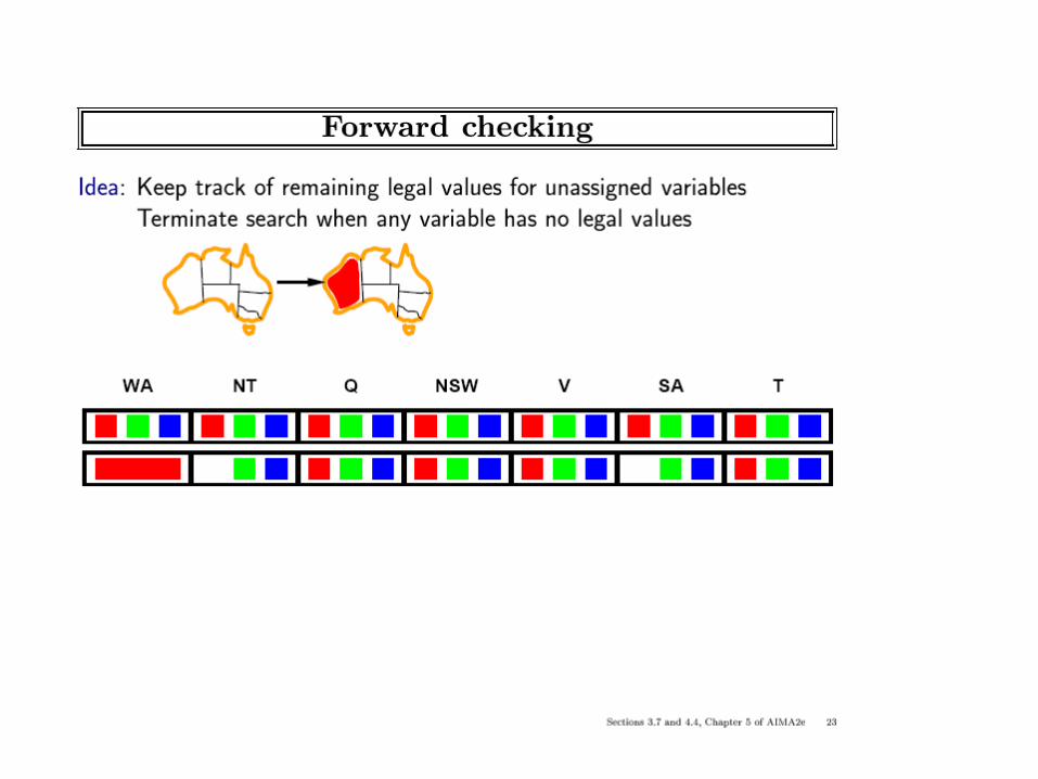
• Forward-checking – (check each unassigned variable separately
• Maintaining arc-consistency (MAC) – (apply full arc-consistency)

ICS-271:Notes 5: 44
ICS-271:Notes 5: 45

ICS-271:Notes 5: 46
ICS-271:Notes 5: 47
ICS-271:Notes 5: 48
ICS-271:Notes 5: 49

ICS-271:Notes 5: 50
ICS-271:Notes 5: 51
ICS-271:Notes 5: 52
ICS-271:Notes 5: 53

ICS-271:Notes 5: 54

ICS-271:Notes 5: 55
ICS-271:Notes 5: 57
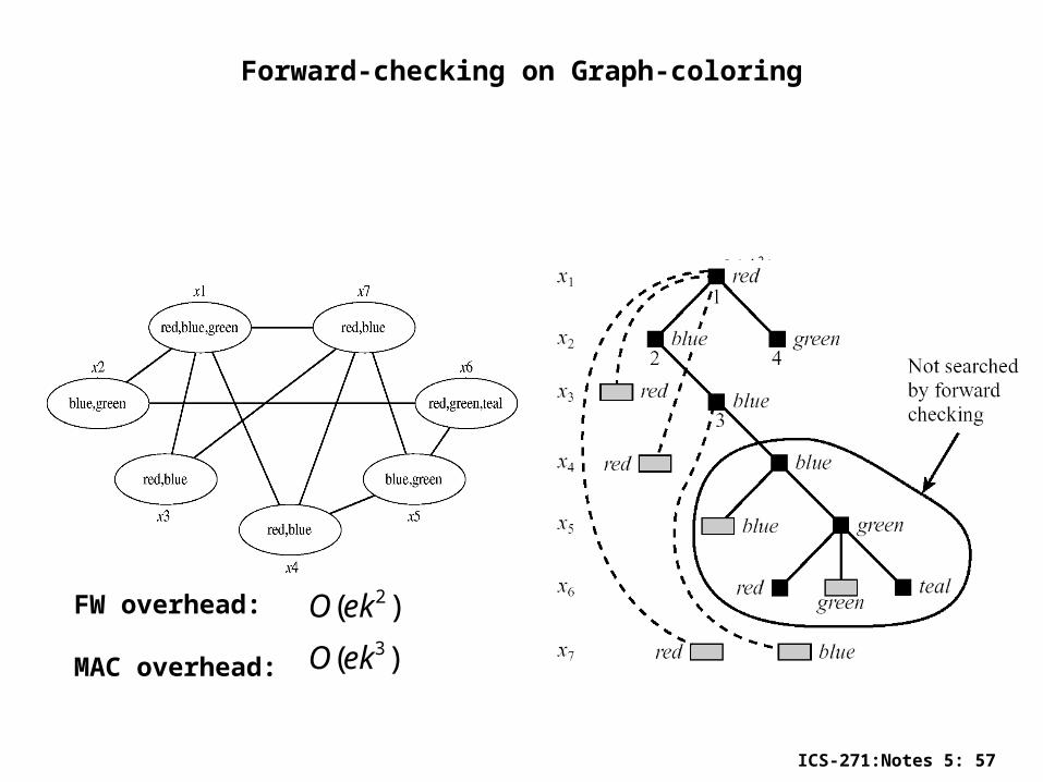
Forward-checking on Graph-coloring
)( 2ekO
)(
)(3
2
ekO
ekOFW overhead:
MAC overhead:

ICS-271:Notes 5: 58
Propositional Satisfiability
• If Alex goes, then Becky goes:• If Chris goes, then Alex goes:• Query:
Is it possible that Chris goes to the party but Becky does not?
Example: party problem
) (or, BA BA ) (or, ACA C
e?satisfiabl Is
C B, A,C B,Atheorynalpropositio
ICS-271:Notes 5: 59
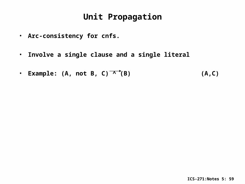
Unit Propagation
• Arc-consistency for cnfs.
• Involve a single clause and a single literal
• Example: (A, not B, C) ^ (B) (A,C)

ICS-271:Notes 5: 60
Look-ahead for SAT(Davis-Putnam, Logeman and Laveland, 1962)

ICS-271:Notes 5: 61
Look-ahead for SAT: DPLLexample: (~AVB)(~CVA)(AVBVD)(C)
Only enclosed area will be explored with unit-propagation
Backtracking look-ahead with Unit propagation= Generalized arc-consistency
(Davis-Putnam, Logeman and Laveland, 1962)

ICS-271:Notes 5: 62
Look-back: Backjumping / Learning
• Backjumping: – In deadends, go back to the most recent culprit.
• Learning: – constraint-recording, no-good recording.
– good-recording
ICS-271:Notes 5: 63
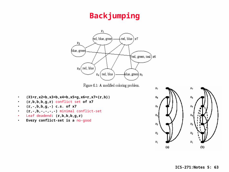
Backjumping
• (X1=r,x2=b,x3=b,x4=b,x5=g,x6=r,x7={r,b})• (r,b,b,b,g,r) conflict set of x7• (r,-,b,b,g,-) c.s. of x7• (r,-,b,-,-,-,-) minimal conflict-set• Leaf deadend: (r,b,b,b,g,r)• Every conflict-set is a no-good
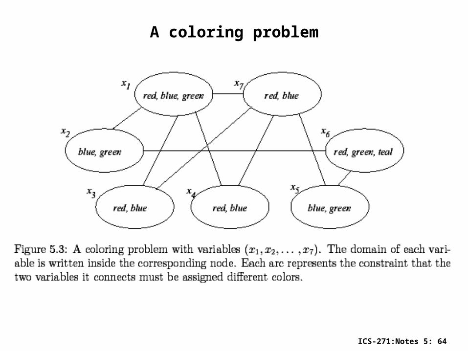
ICS-271:Notes 5: 64
A coloring problem

ICS-271:Notes 5: 66
ICS-271:Notes 5: 67
ICS-271:Notes 5: 68

ICS-271:Notes 5: 69

ICS-271:Notes 5: 70

ICS-271:Notes 5: 71
The cycle-cutset method
• An instantiation can be viewed as blocking cycles in the graph
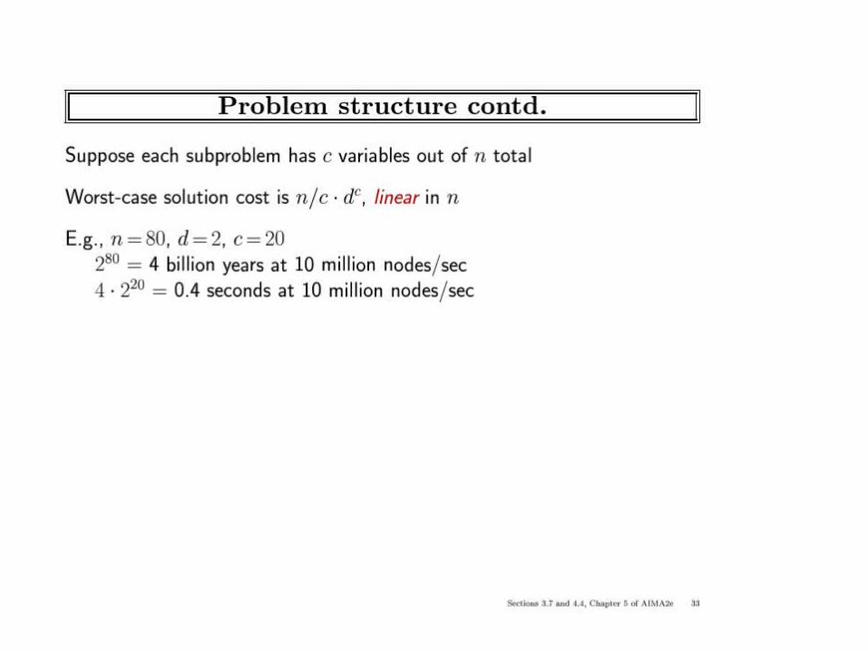
• Given an instantiation to a set of variables that cut all cycles (a cycle-cutset) the rest of the problem can be solved in linear time by a tree algorithm.
• Complexity (n number of variables, k the domain size and C the cycle-cutset size):
)( 2knkO C

ICS-271:Notes 5: 72
Tree Decomposition

ICS-271:Notes 5: 73

ICS-271:Notes 5: 74

ICS-271:Notes 5: 75

ICS-271:Notes 5: 76
GSAT – local search for SAT(Selman, Levesque and Mitchell, 1992)
1. For i=1 to MaxTries
2. Select a random assignment A
3. For j=1 to MaxFlips
4. if A satisfies all constraint, return A
5. else flip a variable to maximize the score
6. (number of satisfied constraints; if no variable
7. assignment increases the score, flip at random)
8. end
9. end
Greatly improves hill-climbing by adding restarts and sideway moves
ICS-271:Notes 5: 77
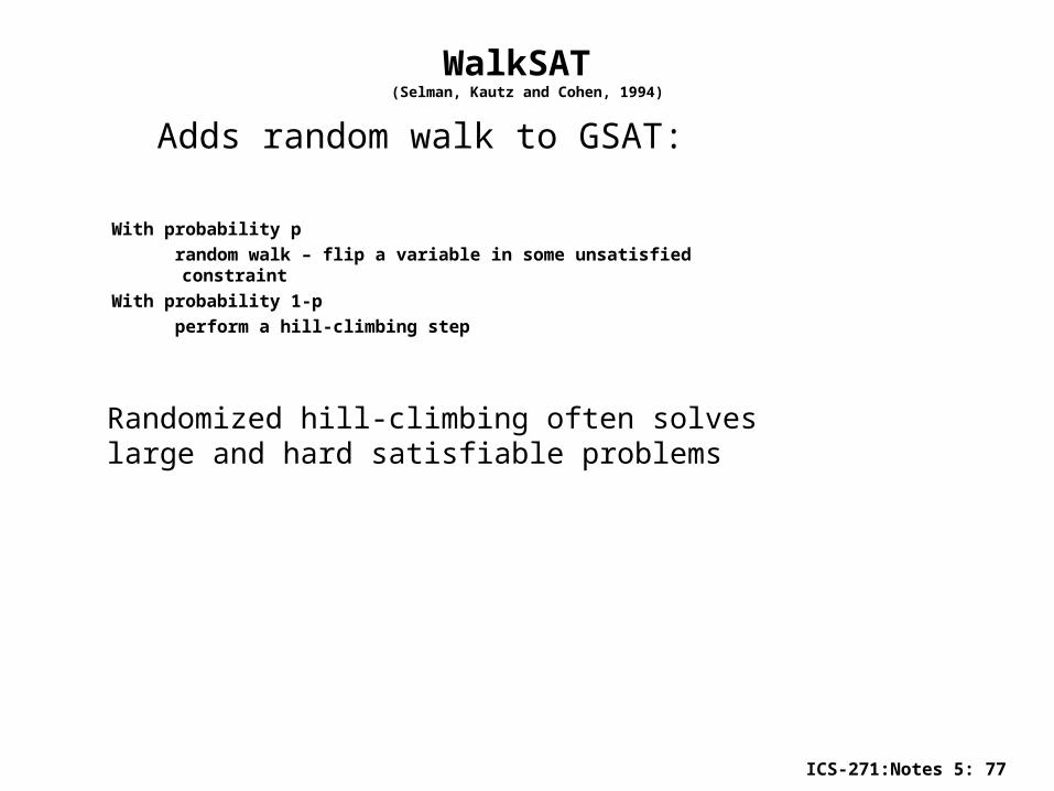
WalkSAT (Selman, Kautz and Cohen, 1994)
With probability p
random walk – flip a variable in some unsatisfied constraint
With probability 1-p
perform a hill-climbing step
Adds random walk to GSAT:
Randomized hill-climbing often solves large and hard satisfiable problems

ICS-271:Notes 5: 78
More Stochastic Search: Simulated Annealing, reweighting
• Simulated annealing:
– A method for overcoming local minimas
– Allows bad moves with some probability:
• With some probability related to a temperature parameter T the next move is picked randomly.
– Theoretically, with a slow enough cooling schedule, this algorithm will find the optimal solution. But so will searching randomly.
• Breakout method (Morris, 1990): adjust the weights of the violated constraints
ICS-271:Notes 5: 79