IDENTIFICATION OF DEGRADED LOTIC FRESHWATER THAT AFFECTS

IDENTIFICATION OF DEGRADED LOTIC FRESHWATER THAT AFFECTS SALMON HABITAT, SHELLFISH BEDS AND RECREATION IN SOUTH PUGET

SOUND USING WATER QUALITY DATA AND LAND USE ANALYSIS

by Don Loft

A Thesis-Essay of Distinction Submitted in Partial Fulfillment

of the requirements for the degree Master of Environmental Studies

The Evergreen State College July 2012

© 2012 by Don Loft. All rights reserved.

This Thesis for the Master of Environmental Studies Degree

by

Don Loft

has been approved for

The Evergreen State College

by

__________________________________ Judith Bayard Cushing, Ph.D.

_______________________ Date

ABSTRACT

Identification of Degraded Lotic Freshwater that Affects Salmon Habitat, Shellfish Beds and Recreation in South Puget Sound Using Water Quality Data and Land Use Analysis

Don Loft

Ecosystems are becoming degraded through human activity and neglect, resulting

in the decline of productive habitats, increasing levels of toxins and a threat of species extinction. The quality of water in aquatic habitats is essential, because water is the basis for all life. To improve the health of an ecosystem, we must maintain the quality of water that sustains it. The purpose of this thesis project was to use water quality standards to identify habitats with degraded water quality for key species of salmonids, shellfish beds, as well as human recreation.

This research will answer the following questions: 1) Which water quality parameters define healthy and sustainable salmon habitats in lotic freshwater systems? 2) By using water quality standards as criteria, which freshwater lotic systems are degraded in two South Puget Sound watersheds? 3) What are the degrading effects of different types of land use and impervious surfaces having on water discharging from drainage systems into creeks, streams and wetlands?

This study focused on two watersheds in Western Washington’s South Puget Sound, WRIA 11 (Nisqually) and WRIA 13 (Deschutes), and utilized water quality data analysis and geographic information system (GIS) to map the analysis results. The next level of analysis used the GIS hydrology tools to define the flow basins and identify land use features within those flow basins. This was performed on those sites considered to have highly degraded water quality. The selected flow basins were used to identify land use that could potentially affect water quality and degrade habitat.

The analysis compared existing water quality data against the Washington State Department of Ecology water quality standards to develop a color coded tier ranking system based on how often the data failed to meet the criteria standards. The ranking system resulted in an enhanced method for the identification of degraded and healthy lotic freshwater systems. The methods used in this thesis project produced a valuable tool, graphically representing potential target areas for salmon recovery and habitat restoration and enhancement.

iv

Table of Contents

PageList of Figures ……………………………………………………………………….. viiList of Tables ……………………………………………………………………....... viiiAcknowledgments ………………………………………………………………....... x Chapter One: Water Quality Standards, Criteria and Methods of Analysis for Two Watersheds in South Puget Sound ………………………………………………… 1Introduction …………………………………………………………………………. 1Area of Study ………………………………………………………........................... 2 Nisqually River Basin (WRIA 11) ……………………………………............ 3 Fish Species and Habitat (WRIA 11) ……………………………………........ 3 Deschutes River Basin (WRIA 13) …………………………………………... 4 Fish Species and Habitat (WRIA 13) ……………………………………........ 4 WDFW Salmonid Stock Inventory ………………………………………....... 5Water Quality Standards ………………………………………………………....... 6 Dissolved Oxygen ……………………………………………………………. 6 Bacteria Levels ……………………………………………………………….. 6 Turbidity …………………………………………………………………........ 7 pH ……………………………………………………………………….......... 7 Temperature ………………………………………………………………...... 8Data Analysis ……………………………………………………………………....... 9 Source of Data …………………………………………………………........... 9 Data Organization ……………………………………………………………. 9Methods …………………………………………………………………………........ 10 Tabular Data Analysis ……………………………………………………....... 10 Aggregation of Ranking Results …………………………………………....... 16 GIS Spatial Data and Join Tables ……………………………………………. 17 Chapter Two: Identification of Degraded Habitat in Lotic Freshwater Systems ……………….. 19Results and Conclusions ……………………………………………………………. 19 Results for WRIA 11 …………………………………………………………. 20 DO Results …………………………………………………………… 20 FC 50 cfu Results …………………………………………………….. 21 FC 100 cfu Results …………………………………………………… 21 Turbidity Results ……………………………………………………... 22 Temperature Results …………………………………………………. 23 Results for WRIA 13 …………………………………………………………. 27 DO Results …………………………………………………………… 27 FC 50 cfu Results …………………………………………………….. 28

v

Table of Contents (Continued)

PageChapter Two (Continued) FC 100 cfu Results …………………………………………………… 29 Turbidity Results ……………………………………………………... 31 pH Results ……………………………………………………………. 31 Temperature Results …………………………………………………. 32 Final Site Selection for Degraded Water Quality ……………………………. 37 WRIA 11 Lotic Systems ……………………………………………... 38 WRIA 11 Lentic Systems ……………………………………………. 40 WRIA 11 Lotic System Tide Gates ………………………………….. 40 WRIA 11 FC in Lotic Systems ………………………………………. 42 WRIA 13 Lotic Systems ……………………………………………... 43 WRIA 13 Lentic Systems ……………………………………………. 44 WRIA 13 FC in Lotic Systems ………………………………………. 45 Conclusions WRIA 11 ……………………………………………………….. 46 Conclusions WRIA 13 ……………………………………………………….. 46 Chapter Three: Anthropogenic Land Use and Impervious Surfaces Adjacent to Salmon Habitat and Shellfish Beds …………………………………………………………………... 48Introduction …………………………………………………………………………. 48Natural Systems vs. Developed Systems …………………………………………... 49Land Use and Estuarine Habitats …………………………………………………. 50Threats to Puget Sound Shellfish …………………………………………………... 51Impact of Development and Fecal Coliform ………………………………………. 52Reports and Surveys ………………………………………………………………... 53Classifications ……………………………………………………………………….. 53Criteria ………………………………………………………………………………. 54Study Areas ………………………………………………………………………….. 55Description of Growing Area ………………………………………………………. 55 Nisqually Reach ……………………………………………………………… 55 Henderson Inlet ………………………………………………………………. 56Reports by Washington State Department of Health …………………………….. 56 Nisqually Reach ……………………………………………………………… 56 Henderson Inlet ………………………………………………………………. 57Report by Washington State Department of Ecology …………………………….. 59Land Use …………………………………………………………………………….. 60 Land Use Types ……………………………………………………………… 61 WRIA 11 Parcels …………………………………………………………….. 61 WRIA 13 Parcels …………………………………………………………….. 63Impervious Surfaces ………………………………………………………………... 64 The Problem ………………………………………………………………….. 65

vi

Table of Contents (Continued)

PageChapter Three (Continued) Analysis of the Lower Henderson Inlet Sub-Basin Septic Systems as Source of Fecal Coliform Loading on Shellfish Beds ……………………………………........ 67 Point and Non-Point Source Pollution ……………………………………….. 68 Spatial Analysis ………………………………………………………………. 69 Conclusions …………………………………………………………………... 71 Chapter Four: Defining Flow Basin Influence on Degraded Lotic Systems ……………………... 73Introduction …………………………………………………………………………. 73Watershed Function and Stressors ………………………………………………… 73Spatial Analysis of Ohop Creek in WRIA 11 ……………………………………... 75 Flow Basins …………………………………………………………………... 76 Joining Spatial and Tabular Data …………………………………………….. 78 Flow Basin Analysis …………………………………………………………. 78 Analysis of Flow Basin Land Use …………………………………………… 79 Analysis of Land Use and Water Quality ……………………………………. 82 Conclusions …………………………………………………………………... 84Final Thoughts ………………………………………………………………………. 88References …………………………………………………………………………… 89Appendix …………………………………………………………………………...... 92

vii

List of Figures

Page

Figure 1.1: Washington State Map and Location of Project Watersheds ………......... 3

Figure 2.1: Tide Gate in Westport, Washington ……………………………………... 41

Figure 3.1: The Lower Henderson Inlet Sub-Basin and Shellfish Bed Area ………… 68

Figure 3.2: The 35% FC 50 Monitoring Sites in the Lower Henderson Inlet …........... 69

Figure 3.3: The FC 50 Target Creeks in the Lower Henderson Inlet ………………... 70

Figure 3.4: Target Parcels with Septic Systems in the Lower Henderson Inlet ……… 71

Figure 4.1: The Ohop Flow Basin Feature …………………………………………… 77

Figure 4.2: The Ohop Flow Basin with Land Use Features …………………………. 77

Figure 4.3: Segment A of the Ohop Land Use Analysis …………………………….. 80

Figure 4.4: Segment B of the Ohop Land Use Analysis ……………………………... 80

Figure 4.5: Segment C of the Ohop Land Use Analysis ……………………………... 81

Figure 4.6: Segment D of the Ohop Land Use Analysis …………………………….. 81

Figure 4.7: The Ohop Flow Basin Four Monitoring Sites. …………………………... 83

viii

List of Tables

PageChapter 1 Table 1.1: WDFW’s Salmonid Stock Inventory Stock Status WRIA 11 & 13 ……… 5Table 1.2: WA surface water quality standards DO, FC, Turbidity and pH ……......... 8Table 1.3: Washington State surface water quality standards for Temperature …....... 8Table 1.4: Criteria, Functions and Formulas for DO, FC, pH and Turbidity ………......... 11Table 1.5: Measure of data spread for (Min, Max, Quartiles, & Median) ………........ 12Table 1.6: Criteria, Functions & Formulas Seasonal Use Temperature Analysis …….. 14Chapter 2 Table 2.1: Results for degraded DO levels (geo mean < 8mg/L) WRIA 11 …………. 20Table 2.2: Results for degraded FC levels (geo mean > 50 cfu) WRIA 11 ………….. 21Table 2.3: Results for degraded FC levels (geo mean > 100 cfu) WRIA 11 ………… 22Table 2.4: Results for degraded turbidity levels (geo mean > 7.8 NTU) WRIA 11 …. 23Table 2.5: All Year Temperature Results for Char Rearing WRIA 11 ………………. 24Table 2.6: F/W/Sp Temperature Results for Salmon & Trout WRIA 11 ……………. 25Table 2.7: Summer Temperature Results for the Core Salmonid WRIA 11 ………… 26Table 2.8: Fall Temperature Results for the Char Spawning WRIA 11 ……………... 27Table 2.9: Results for degraded DO levels (geo mean < 8mg/L) WRIA 13 …………. 28Table 2.10: Results for degraded FC levels (geo mean > 50 cfu) WRIA 13 ………… 29Table 2.11: Results for degraded FC levels (geo mean > 100 cfu) WRIA 13 ……….. 30Table 2.12: Results for degraded turbidity levels (geo mean > 6.8 NTU) WRIA 13 ... 31Table 2.13: Results for degraded pH levels (geo mean < 6.5 or > 8.5) WRIA 13 …… 32Table 2.14: All Year Temperature Results for Char Rearing WRIA 13 ……………... 34Table 2.15: F/W/Sp Temperature Results for Salmon & Trout WRIA 13 …………... 35Table 2.16: Summer Temperature Results for the Core Salmonid WRIA 13 ……….. 36Table 2.17: Fall Temperature Results for the Char Spawning WRIA 13 ……………. 37Table 2.18: Aggregated Lotic Results Across Multiple Parameters WRIA 11 …........ 39Table 2.19: Aggregated Lentic Results Across Multiple Parameters WRIA 11 ……... 40Table 2.20: Aggregated Tide Gate Results Across Multiple Parameters WRIA 11 …. 42Table 2.21: Aggregated Fecal Coliform Results Across Two Parameters WRIA 11 ... 43Table 2.22: Aggregated Lotic Results Across Multiple Parameters WRIA 13 ……… 44Table 2.23: Aggregated Lentic Results Across Multiple Parameters WRIA 13 ……... 45Table 2.24: Aggregated Fecal Coliform Results Across Two Parameters WRIA 13 ... 47Chapter 3 Table 3.1; DOH Sites Not Meeting Water Quality Standards For Nisqually Reach … 57Table 3.2: DOH Sites Not Meeting Water Quality Standards For Henderson Inlet …. 57Table 3.3: Sites Classified As Conditionally Approved Plus Two Approved Sites …. 58Table 3.4: Creeks Not Meeting TMDL Standards …………………………………… 59Table 3.5: Totals for Land Use Type in WRIA 11 ………………………………….. 62Table 3.6: Totals for Land Use Type by County in WRIA 11 ……………………... 62

ix

List of Tables (Continued)

PageChapter 3 (Continued) Table 3.7: Totals for Land Use Type in WRIA 13 ………………………………….. 63Table 3.8: Totals for Land Use Types by County in WRIA 13 …………………….. 64Chapter 4 Table 4.1: Ohop Creek Site Selections ………………………………………………. 75Table 4.2: Ohop Flow Basin Calculated Land –Use …………………………………. 78Table 4.3: Aggregated Water Quality Results for the Ohop Monitoring Sites ………. 83Table 4.4: Site 4 Water Quality Result Ranking, Segment D Land Use Totals ……... 84Table 4.5: Site 3 Water Quality Result Ranking, Segment C Land Use Totals ……... 85Table 4.6: Site 2 Water Quality Result Ranking, Segment B Land Use Totals ……... 87Table 4.7: Site 1 Water Quality Result Ranking, Segment A Land Use Totals ……... 87Appendix Table A1: Lotic Site Locations WRIA 11 …………………………………………… 92Table A2: Lentic Site Locations WRIA 11 …………………………………………... 93Table A3: Lotic System Tide Gate Locations WRIA 11 …………………………….. 93Table A4: Lotic Site Locations WRIA 13 …………………………………………… 94Table A5: Lentic Site Locations WRIA 13 …………………………………………... 95

x

Acknowledgements

The first person I would like to acknowledge is Randy Lehr, Ph.D. for first guiding me on the path of identifying degraded freshwater systems through the analysis of water quality data. My work on the Chehalis River Basin Water Quality Project with Mr. Lehr provided the rudimentary foundation for my thesis project. My second partner in the Chehalis River Basin Water Quality Project was Joel Green, Ph.D. His expertise in fish biology helped me to refine my focus on the fundamental water quality parameters that support seasonal use by a variety salmonid species in aquatic habitats. Green played an important role in proofing the data for outliers and statistical analysis. He also performed the major role in the State-of-the-River report we co-authored. The next acknowledgements go to people who supported my original water quality project for the Chehalis Basin. My thanks and admiration goes to the following people: Mike Kelly (Grays Harbor College) for his friendship and facilitating my contract to study the water quality in the Chehalis Basin. Janel Spaulding (Chehalis Basin Partnership) for her support and networking which supported my project. David Rountry (Department of Ecology) for his guidance on water quality issues and standards. Harry Pickernell (Water Resources Specialist The Chehalis Tribes) for the water quality data supplied for my project and his expertise as field research and lab methods.

I would now like to acknowledge those people who were instrumental in the creation and support of my thesis project. When I entered the MES program, I had a fairly good idea where I wanted to take it. Through the support of many professors and fellow students in my undergrad and graduate programs helped me clarify my thesis objectives. Special thanks to: Dylan Fischer, Ph.D., Rob Knapp, Ph.D., Rob Cole, Ph.D., Martha Henderson, Ph.D., Ralph Murphy, Ph.D., Timothy Quinn, Ph.D., Alison Styring, Ph.D., Anna Wederspahn, MES, Tim Benedict, MES, Noel Ferguson, MES, Chris Holcomb, MES, Nahal Ghoghaie, MES, Scott Morgan (Office of Sustainability), Gavin Glore (Mason Conservation District), and Jerilyn Walley, MES for support and proof reading my thesis.

For help in GIS spatial analysis for hydrology, I would like to give my thanks to

Greg Stewart, Ph.D. for all his help and guidance. Thanks to Gerardo Chin-Leo, Ph.D. for his help in crafting and organizing my thesis from prospectus to thesis project. Special thanks goes to Gail Wootan (Assistant Director to the MES Program) for her gentle and caring support to get my thesis to the goal line.

My utmost gratitude goes to my esteemed thesis reader Judith Cushing, Ph.D.

whose help and guidance got me to the finish line. Her input was invaluable, her support unwavering. When I got off track, she nudged me back on path. Judith’s support and suggestions on methods and refinements has made the crafting of my thesis a pleasure to accomplish. I could not have picked a better person to be my thesis reader. I am a better graduate student for having known her.

1

Chapter One:

Water Quality Standards, Criteria and Methods of Analysis for Two Watersheds in

South Puget Sound

Introduction: The key element to assessing the health of salmon habitat is the collection of

reliable data on that habitat. If there are no existing data for a habitat sustainability study,

then field work is needed to obtain samples to analyze. When data are available on the

study area’s lotic freshwater salmon habitat, it is often obtained from many of the

stakeholders in the area, and that can range from state and federal environmental agencies

as well and local tribes and conservation districts. For this study data were acquired from

The Washington State Department of Ecology, which maintains a large database

collected from stakeholders from all regions in the state. The data used in this study were

downloaded from their Environmental Information Management System (EIM) for two

watersheds in the South Puget Sound area. Watersheds in Washington State are referred

to as Water Resource Inventory Areas (WRIA) which defines the flow direction of runoff

water from rainfall and snow melt. The salmon habitats in lotic freshwater systems in this

study are WRIA 11 (Nisqually) and WRIA 13 (Deschutes).

Water quality data are used to determine if any salmon habitats or recreational

streams have become degraded and for potential impact on shellfish. The water quality

parameters used in this study are dissolved oxygen, fecal coliform, turbidity, pH and

temperature. These data will undergo analysis that compares the data against the water

quality standards outlined in the Clean Water Act and by The Washington State

Department of Ecology. The criteria for high water quality standards will be used to

compare samples taken at specific monitoring sites and then ranked by percentage of time

the samples do not meet the criteria. A second level of criteria for low water quality

standards will be used for some of the parameters, as this is needed for some species

habitat requirements. This ranking will be graphically represented in a geographic

2

information system (GIS) format. Monitoring sites showing the highest percentage of

times not meeting the criteria will be given further analysis of the flow basins to those

sites and the land use within those flow basins.

This thesis project produced enhanced methods for identifying degraded lotic

streams, creeks and drainage of freshwater systems. This was accomplished through the

use of water quality data analysis and applying those findings to GIS maps. GIS

hydrology tools were used to identify land use features within flow basins that could

potentially affect the water quality results found at specific monitoring sites. This

information could be used to target potential habitat restoration and mitigation projects.

The defined flow basins for these sites could also assist in assembling strategies for a

more in-depth research within troubled habitats.

Area of Study:

This study took place in the Pacific Northwest and focused on two watersheds

that discharge runoff water into Puget Sound. The Puget Sound, in the western part of

Washington State, is a large estuarine system carved out by the advancement and

receding of the last glacial age over 13,000 years ago. The approximate mile thick glacial

ice stretched down from Canada to what is now near the State Capitol of Washington,

with the Olympic Mountains to the west and the Cascades to the east. The retreating

glacier scoured the landscape leaving behind many lakes, rivers and streams that now

shed runoff water, melting ice and snow from the mountains and hills surrounding Puget

Sound on the east, west and south. The north end of the Puget Sound opens to oceanic

saltwater of the Pacific through the Strait of Juan de Fuca (Ecy, 2011).

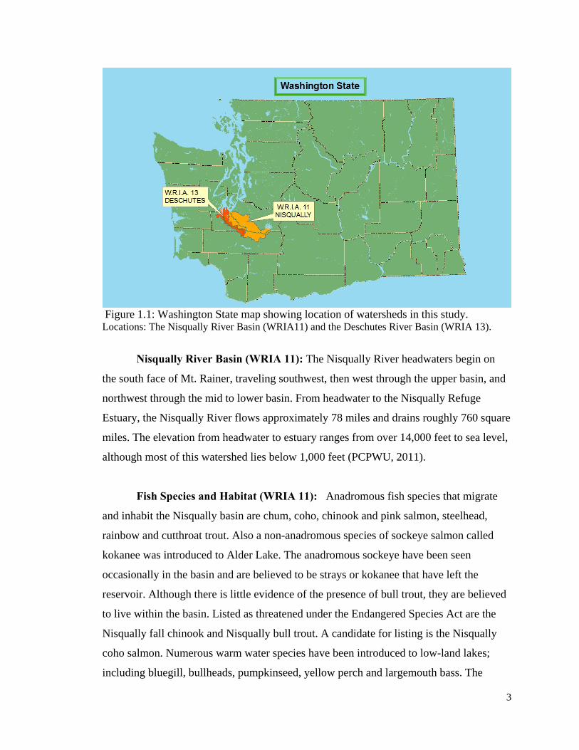
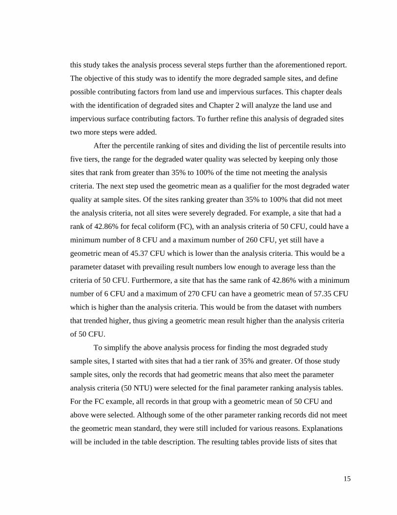
The two watersheds in this study are located at the south end of Puget Sound; the

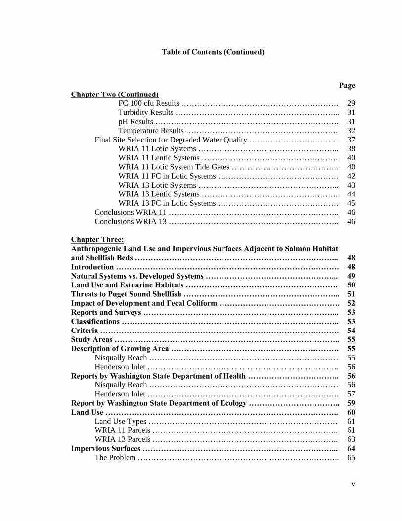
Nisqually (WRIA 11) and the Deschutes (WRIA 13). The Washington State map shown

in Figure 1.1 defines the location of WRIA 11 and WRIA 13 in relation to South Puget

Sound and respectively to each other. These watersheds were chosen because of the

different land uses respective to each.

3

Figure 1.1: Washington State map showing location of watersheds in this study. Locations: The Nisqually River Basin (WRIA11) and the Deschutes River Basin (WRIA 13).

Nisqually River Basin (WRIA 11): The Nisqually River headwaters begin on

the south face of Mt. Rainer, traveling southwest, then west through the upper basin, and

northwest through the mid to lower basin. From headwater to the Nisqually Refuge

Estuary, the Nisqually River flows approximately 78 miles and drains roughly 760 square

miles. The elevation from headwater to estuary ranges from over 14,000 feet to sea level,

although most of this watershed lies below 1,000 feet (PCPWU, 2011).

Fish Species and Habitat (WRIA 11): Anadromous fish species that migrate

and inhabit the Nisqually basin are chum, coho, chinook and pink salmon, steelhead,

rainbow and cutthroat trout. Also a non-anadromous species of sockeye salmon called

kokanee was introduced to Alder Lake. The anadromous sockeye have been seen

occasionally in the basin and are believed to be strays or kokanee that have left the

reservoir. Although there is little evidence of the presence of bull trout, they are believed

to live within the basin. Listed as threatened under the Endangered Species Act are the

Nisqually fall chinook and Nisqually bull trout. A candidate for listing is the Nisqually

coho salmon. Numerous warm water species have been introduced to low-land lakes;

including bluegill, bullheads, pumpkinseed, yellow perch and largemouth bass. The

4

primary salmon habitat is found in the subbasins Mashel, Muck/Murry, and the

Tanwax/Kreger/Ohop. Salmonids also utilize the main channel of the Nisqually River.

Access to other subbasins is limited because of natural and manmade barriers

(WPN, 2002).

Deschutes River Basin (WRIA 13): The headwaters of the Deschutes River

begin in Cougar Mountain at an elevation of 3,870 feet above sea-level, and flows

through steep terrain in Lewis County to the rolling topography of the mid-waters in

Thurston County and to the relatively flat grassy prairies and urban areas. The Deschutes

River discharges about 60% of WRIA 13, approximately 270 square miles. The

remainder of WRIA 13 discharges directly into Puget Sound. The Deschutes River

discharges into Capitol Lake impoundment in downtown Olympia before entering Budd

Inlet of South Puget Sound (WA Ecology, 2005). Percival Creek also discharges into

Capitol Lake and not the main stem of the Deschutes River. WRIA 13 also contains two

large flow basins that do not discharge directly into the main channel of the Deschutes

River, Capitol Lake or Budd Inlet. To the west of Budd Inlet is Eld Inlet, and to the east,

Henderson Inlet. Eld Inlet receives runoff water from McLane, and Swift Creeks at the

southernmost tip, and Green Cove Creek which drains runoff from Cooper Point.

Henderson Inlet receives runoff discharge from two main channels, the Woodland and

Woodard Creeks, which both originate in dense urban areas of Olympia and Lacey.

Dobbs, Meyer, Myer and Goose Creeks are several smaller creeks that discharge from

less dense urban and more rural areas into Henderson Inlet.

Fish Species and Habitat (WRIA 13): With assistance from Native Tribes and

tribal organizations, the Washington State Department of Fish and Wildlife (WDFW)

publishes the State Salmon and Steelhead Stock Inventory (SASSI) report on the

condition of local and introduced fish species. The information used here is from the

Deschutes River Watershed Initial Assessment (Draft May 1995). The SASSI states that

the Deschutes River watershed supports three salmon species, the chum, chinook, and

coho in addition to the winter steelhead. Also utilizing WRIA 13 are the Henderson Inlet

5

fall chum, McLane Creek steelhead and a variety of other fish including Dolly Varden,

sea-run cutthroat trout, pygmy whitefish and Olympic mudminnow (Ecy-2, 2011).

WDFW Salmonid Stock Inventory: WDFW’s Salmonid Stock Inventory (SaSI)

issues reports on the health of salmonids species throughout Washington State. The SaSI

is a tool developed by Native Tribes and WDFW to inventory and monitor Washington’s

salmonids species, because of their cultural and commercial importance to the state’s

ecosystems and its people. The inventory data is compiled on all wild salmonid species

and is assessed to determine if the stock is healthy, depressed, critical, extinct, or

unknown. This results in a recovery action plan to prioritize restoration. Anthropogenic

activities have placed heavy pressures on salmonid stocks through urban development,

industry, forestry, agriculture, overfishing and hydropower dams to name a few. Many of

Washington’s species have become imperiled over time. As of 2002, out of the 598

species that have been identified, 180 are rated as healthy, 132 as depressed, 26 as

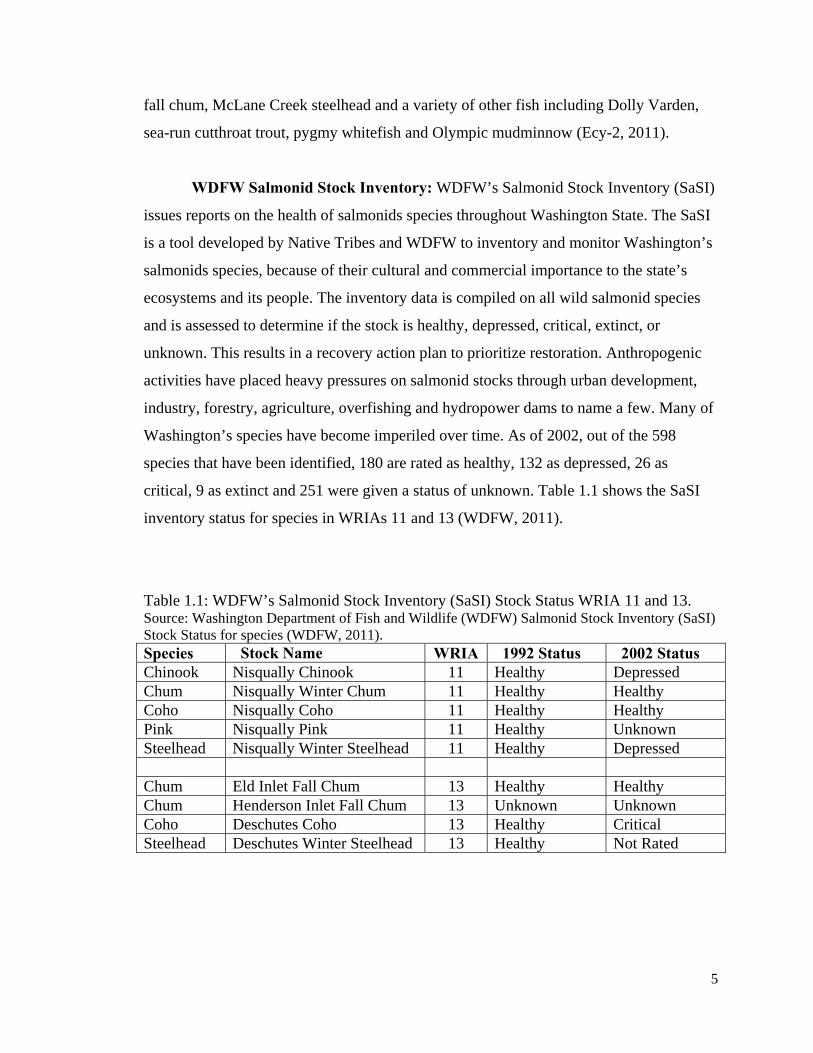
critical, 9 as extinct and 251 were given a status of unknown. Table 1.1 shows the SaSI

inventory status for species in WRIAs 11 and 13 (WDFW, 2011).

Table 1.1: WDFW’s Salmonid Stock Inventory (SaSI) Stock Status WRIA 11 and 13. Source: Washington Department of Fish and Wildlife (WDFW) Salmonid Stock Inventory (SaSI) Stock Status for species (WDFW, 2011). Species Stock Name WRIA 1992 Status 2002 Status Chinook Nisqually Chinook 11 Healthy Depressed Chum Nisqually Winter Chum 11 Healthy Healthy Coho Nisqually Coho 11 Healthy Healthy Pink Nisqually Pink 11 Healthy Unknown Steelhead Nisqually Winter Steelhead 11 Healthy Depressed Chum Eld Inlet Fall Chum 13 Healthy Healthy Chum Henderson Inlet Fall Chum 13 Unknown Unknown Coho Deschutes Coho 13 Healthy Critical Steelhead Deschutes Winter Steelhead 13 Healthy Not Rated

6

Water Quality Standards: The dependent variable is water quality in streams, creeks and drainage systems

that support salmonid rearing and spawning habitats as well as a healthy water quality

fecal coliform standard for shellfish and recreational purposes. The measure of water

quality in lotic systems was determined by freshwater parameters for sustainable

salmonid spawning and rearing habitats, as outlined by the Department of Ecology’s

Water Quality Standards for Surface Water of the State of Washington, Chapter 173-

201A WAC (WA Ecology, 2006). Water quality parameters used in this Thesis (with

corresponding tables referenced in the above mentioned publication) are: dissolved

oxygen (Table 200 (1)(d)), bacteria levels (Table 200 (2)(b)), turbidity (Table 200 (1)(e)),

temperature (Table 200 (1)(c)) and pH (Table 200 (1)(g)). The criteria used for analysis

are those defined in Washington State water quality standards 173-201A WAC, and are

outlined below:

Dissolved Oxygen: Dissolved oxygen levels can be influenced by water

temperature and the large die-off and decay of organic plant material and algae. Stagnant

water or stream water flow that lacks a rough substrate for mixing can also be the cause

of low dissolved oxygen levels. The water quality standards for dissolved oxygen levels

are: 8 mg/L (Low Standard) or above in streams and creeks are necessary to support

salmon spawning and rearing, and 9.5 mg/L (High Standard) or above are needed to

support char and trout (WA Ecology, 2006).

Bacteria Levels: Elevated bacterial levels in stream water can cause problems

such as eutrophication from the growth and decay of plants and algae which depletes

dissolved oxygen. Also, higher bacteria levels can increase stream turbidity as well as

bacterial diseases. Water quality data collected for fecal coliform (FC) was from

Ecology’s EIM database. The standard of measurement is colony forming units (cfu). The

standards used for analysis were the high standard of 50 cfu/100 ml for exceptional water

quality to protect stream water discharge over shellfish beds, and the lower standard of

100 cfu/100 ml to protect recreational primary contact (Green, et al., 2009). Long-term

testing at a sampling site that receives a geometric mean over 100 cfu/100 ml with at least

7

10% of the sample data above 100 cfu/100 ml gets placed on the 303(d) listing. This is

used for a Total Maximum Daily Load (TMDL) study to find and correct point source(s)

of bacteria in fresh surface water (WA Ecology, 2006).

Turbidity: High water quality standards for streams and creeks measure for

5 Nephelometric Turbidity Units (NTU) above background turbidity for individual rivers,

streams and creeks. When water gets to elevated levels of suspended solids, it can have

several adverse effects on fish in spawning and rearing habitats. Turbid water dissuades

fish from taking advantage of habitats because of irritation caused to their gills. Also,

suspended solids settle out over stream beds, covering suitable substrate for laying eggs.

Turbidity decreases the amount of light that is received by benthic plants and algae, thus

decreasing productivity that supports invertebrate habitat and food supply (WA Ecology,

2006).

pH: The high and low standards for pH are between 6.5 and 8.5. Water quality

standards for pH are a factor in the health of lotic systems, but will not be the primary

focus of this research. In future work pH may be utilized if needed for a more in depth

analysis.

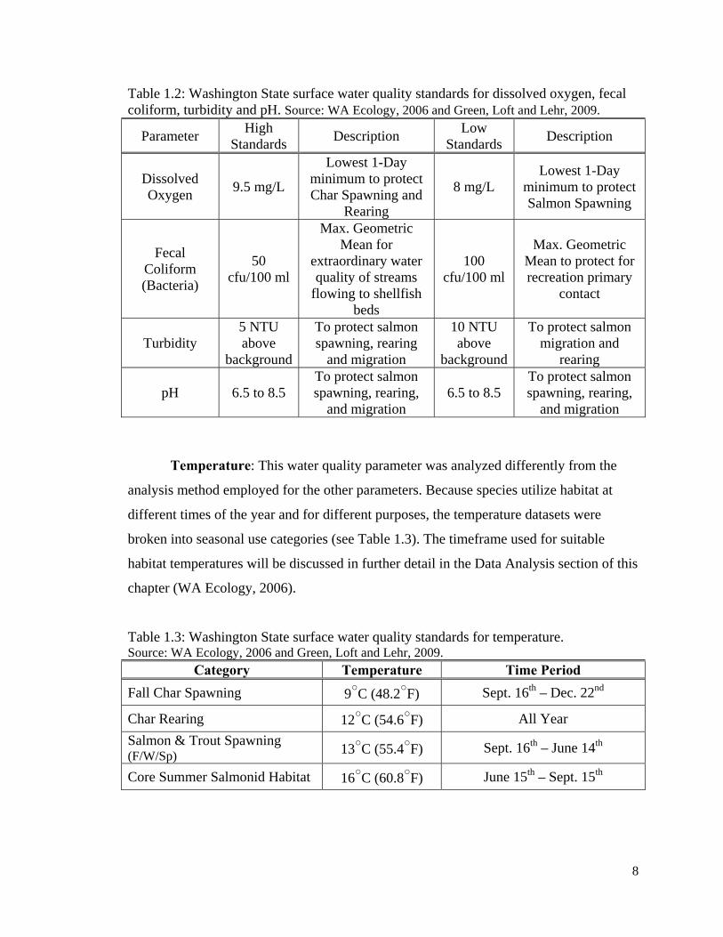
The Washington State standards for surface water quality parameters for

dissolved oxygen, fecal coliform, turbidity and pH, have been summarized in Table 1.2

below. For this study the numerical values of these standards were used as the criteria for

analysis. These standards have two levels of protection. The high standards are adopted

for high or extraordinary fresh surface water quality to protect char and salmon habitats

for spawning, rearing, migration and to protect shellfish from stream water discharge

over shellfish beds. The low standards are adopted to protect dissolved oxygen levels for

salmon spawning, bacteria levels for recreational primary contact protection and turbidity

levels to protect salmon migration and rearing. The pH range is the same for both high

and low standards.

8

Table 1.2: Washington State surface water quality standards for dissolved oxygen, fecal coliform, turbidity and pH. Source: WA Ecology, 2006 and Green, Loft and Lehr, 2009.

Parameter High

Standards Description

Low Standards

Description

Dissolved Oxygen

9.5 mg/L

Lowest 1-Day minimum to protect Char Spawning and

Rearing

8 mg/L Lowest 1-Day

minimum to protect Salmon Spawning

Fecal Coliform (Bacteria)

50 cfu/100 ml

Max. Geometric Mean for

extraordinary water quality of streams

flowing to shellfish beds

100 cfu/100 ml

Max. Geometric Mean to protect for recreation primary

contact

Turbidity 5 NTU above

background

To protect salmon spawning, rearing

and migration

10 NTU above

background

To protect salmon migration and

rearing

pH 6.5 to 8.5 To protect salmon spawning, rearing,

and migration 6.5 to 8.5

To protect salmon spawning, rearing,

and migration

Temperature: This water quality parameter was analyzed differently from the

analysis method employed for the other parameters. Because species utilize habitat at

different times of the year and for different purposes, the temperature datasets were

broken into seasonal use categories (see Table 1.3). The timeframe used for suitable

habitat temperatures will be discussed in further detail in the Data Analysis section of this

chapter (WA Ecology, 2006).

Table 1.3: Washington State surface water quality standards for temperature. Source: WA Ecology, 2006 and Green, Loft and Lehr, 2009.

Category Temperature Time Period

Fall Char Spawning 9○C (48.2○F) Sept. 16th – Dec. 22nd

Char Rearing 12○C (54.6○F) All Year

Salmon & Trout Spawning (F/W/Sp) 13○C (55.4○F) Sept. 16th – June 14th

Core Summer Salmonid Habitat 16○C (60.8○F) June 15th – Sept. 15th

9

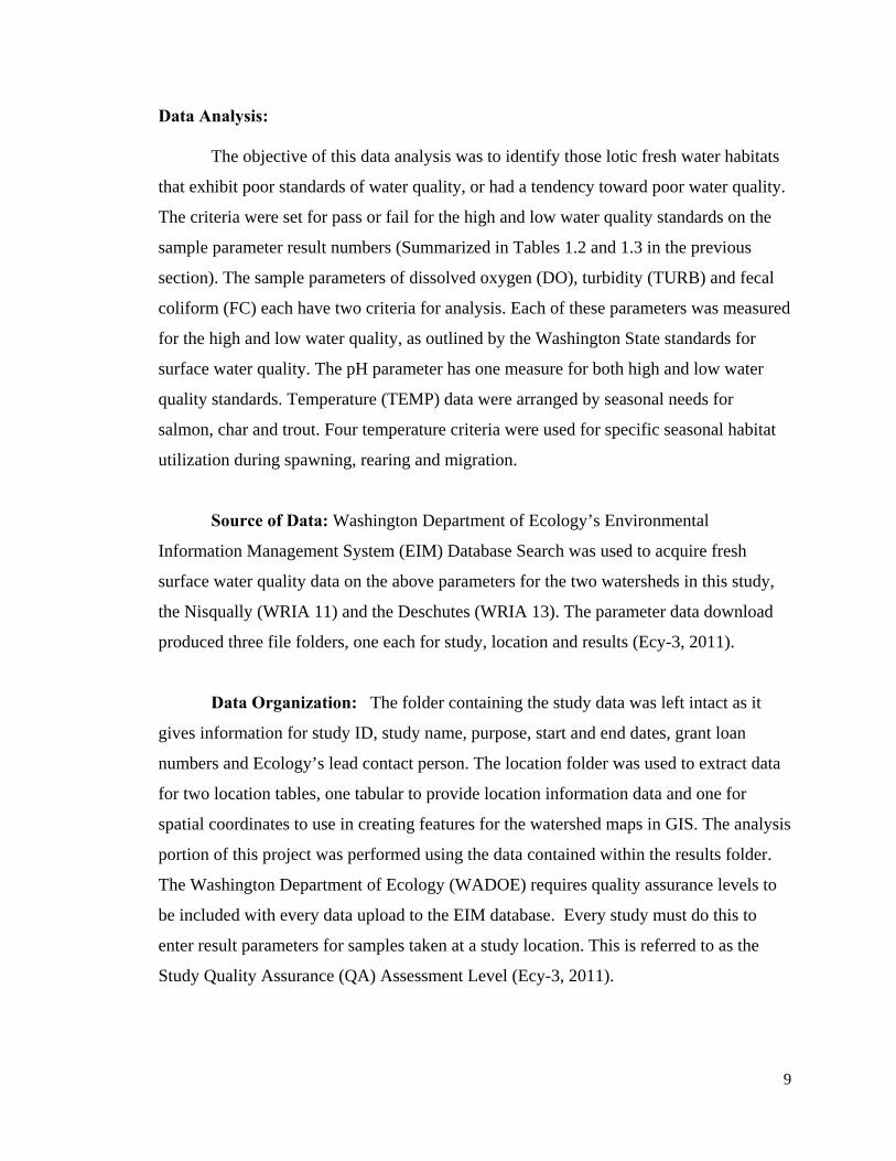
Data Analysis: The objective of this data analysis was to identify those lotic fresh water habitats

that exhibit poor standards of water quality, or had a tendency toward poor water quality.

The criteria were set for pass or fail for the high and low water quality standards on the

sample parameter result numbers (Summarized in Tables 1.2 and 1.3 in the previous

section). The sample parameters of dissolved oxygen (DO), turbidity (TURB) and fecal

coliform (FC) each have two criteria for analysis. Each of these parameters was measured

for the high and low water quality, as outlined by the Washington State standards for

surface water quality. The pH parameter has one measure for both high and low water

quality standards. Temperature (TEMP) data were arranged by seasonal needs for

salmon, char and trout. Four temperature criteria were used for specific seasonal habitat

utilization during spawning, rearing and migration.

Source of Data: Washington Department of Ecology’s Environmental

Information Management System (EIM) Database Search was used to acquire fresh

surface water quality data on the above parameters for the two watersheds in this study,

the Nisqually (WRIA 11) and the Deschutes (WRIA 13). The parameter data download

produced three file folders, one each for study, location and results (Ecy-3, 2011).

Data Organization: The folder containing the study data was left intact as it

gives information for study ID, study name, purpose, start and end dates, grant loan

numbers and Ecology’s lead contact person. The location folder was used to extract data

for two location tables, one tabular to provide location information data and one for

spatial coordinates to use in creating features for the watershed maps in GIS. The analysis

portion of this project was performed using the data contained within the results folder.

The Washington Department of Ecology (WADOE) requires quality assurance levels to

be included with every data upload to the EIM database. Every study must do this to

enter result parameters for samples taken at a study location. This is referred to as the

Study Quality Assurance (QA) Assessment Level (Ecy-3, 2011).

10

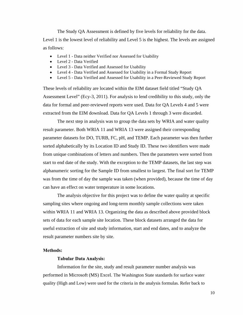
The Study QA Assessment is defined by five levels for reliability for the data.

Level 1 is the lowest level of reliability and Level 5 is the highest. The levels are assigned

as follows:

Level 1 - Data neither Verified nor Assessed for Usability Level 2 - Data Verified Level 3 - Data Verified and Assessed for Usability Level 4 - Data Verified and Assessed for Usability in a Formal Study Report Level 5 - Data Verified and Assessed for Usability in a Peer-Reviewed Study Report

These levels of reliability are located within the EIM dataset field titled “Study QA

Assessment Level” (Ecy-3, 2011). For analysis to lend credibility to this study, only the

data for formal and peer-reviewed reports were used. Data for QA Levels 4 and 5 were

extracted from the EIM download. Data for QA Levels 1 through 3 were discarded.

The next step in analysis was to group the data sets by WRIA and water quality

result parameter. Both WRIA 11 and WRIA 13 were assigned their corresponding

parameter datasets for DO, TURB, FC, pH, and TEMP. Each parameter was then further

sorted alphabetically by its Location ID and Study ID. These two identifiers were made

from unique combinations of letters and numbers. Then the parameters were sorted from

start to end date of the study. With the exception to the TEMP datasets, the last step was

alphanumeric sorting for the Sample ID from smallest to largest. The final sort for TEMP

was from the time of day the sample was taken (when provided), because the time of day

can have an effect on water temperature in some locations.

The analysis objective for this project was to define the water quality at specific

sampling sites where ongoing and long-term monthly sample collections were taken

within WRIA 11 and WRIA 13. Organizing the data as described above provided block

sets of data for each sample site location. These block datasets arranged the data for

useful extraction of site and study information, start and end dates, and to analyze the

result parameter numbers site by site.

Methods:

Tabular Data Analysis:

Information for the site, study and result parameter number analysis was

performed in Microsoft (MS) Excel. The Washington State standards for surface water

quality (High and Low) were used for the criteria in the analysis formulas. Refer back to

11

Tables 1.2 and 1.3 in the Water Quality Standards section. Each site and parameter provided

information on site location, study information and the result parameter numbers taken for

each site. Formulas were created for each site location dataset to acquire the total number of

records, the number of records not meeting the criteria and the percentage of those records

that did not meet the criteria. Also assembled from these records were the study site’s

geometric mean, minimum (smallest) and maximum (largest) from the result parameter

numbers. Other information assembled from each dataset was the QA assurance level, start

date, end date and unique identifiers for the site location and the study. A formula bar was

created for each parameter dataset to organize and assess the information described above.

The algorithms were exported and aggregated for each parameter in each WRIA for this

study. This created join tables for the GIS portion of this analysis, discussed later in this

section. Discussion on the land use and impervious surface GIS procedures for this study are

in following chapters.

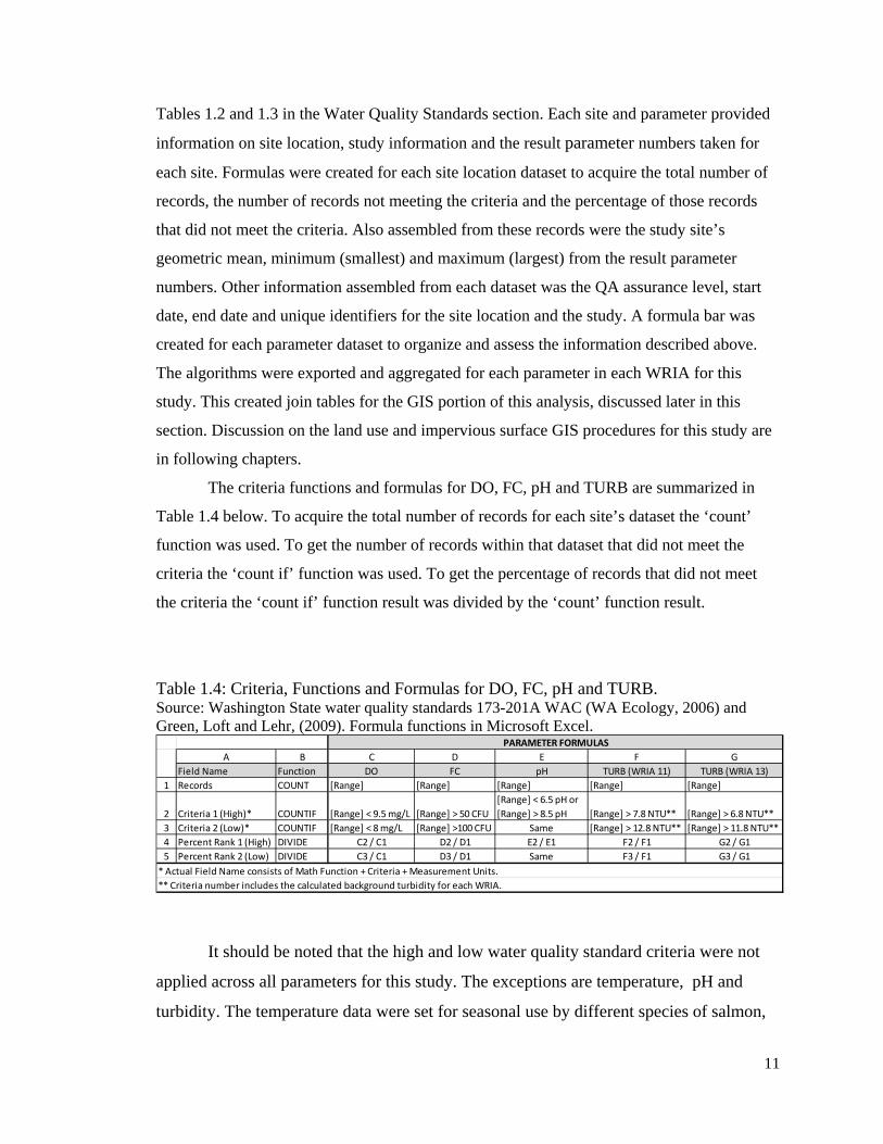
The criteria functions and formulas for DO, FC, pH and TURB are summarized in

Table 1.4 below. To acquire the total number of records for each site’s dataset the ‘count’

function was used. To get the number of records within that dataset that did not meet the

criteria the ‘count if’ function was used. To get the percentage of records that did not meet

the criteria the ‘count if’ function result was divided by the ‘count’ function result.

Table 1.4: Criteria, Functions and Formulas for DO, FC, pH and TURB. Source: Washington State water quality standards 173-201A WAC (WA Ecology, 2006) and Green, Loft and Lehr, (2009). Formula functions in Microsoft Excel.

A B C D E F GField Name Function DO FC pH TURB (WRIA 11) TURB (WRIA 13)

1 Records COUNT [Range] [Range] [Range] [Range] [Range]

2 Criteria 1 (High)* COUNTIF [Range] < 9.5 mg/L [Range] > 50 CFU[Range] < 6.5 pH or [Range] > 8.5 pH [Range] > 7.8 NTU** [Range] > 6.8 NTU**

3 Criteria 2 (Low)* COUNTIF [Range] < 8 mg/L [Range] >100 CFU Same [Range] > 12.8 NTU** [Range] > 11.8 NTU**4 Percent Rank 1 (High) DIVIDE C2 / C1 D2 / D1 E2 / E1 F2 / F1 G2 / G15 Percent Rank 2 (Low) DIVIDE C3 / C1 D3 / D1 Same F3 / F1 G3 / G1

PARAMETER FORMULAS

* Actual Field Name consists of Math Function + Criteria + Measurement Units.** Criteria number includes the calculated background turbidity for each WRIA.

It should be noted that the high and low water quality standard criteria were not

applied across all parameters for this study. The exceptions are temperature, pH and

turbidity. The temperature data were set for seasonal use by different species of salmon,

12

char and trout spawning and rearing habitation. The pH standard for fresh surface water

quality is in a range from 6.5 pH to 8.5 pH. The standard for pH is the same for high or

low water quality. The turbidity high water quality standard is 5 NTU above background,

and the low water quality standard is 10 NTU above background (WA Ecology, 2006).

For this study only the high water quality standard was used for the turbidity analysis.

The low water quality standard was used only to identify those sites of extreme turbidity.

Background turbidity is somewhat unique to each lotic system. Different background

levels can be influenced by soil types and streambed substrates. The typical measure for

background levels is to sample the turbidity of a stream above a disturbance site to gain

normal stream function turbidity levels. Examples of a disturbance include timber

practices, road construction, culvert removal or replacemant and stream modification.

To establish background turdibity for this study a different metric needed to be

applied. Instead of monitoring turbidity at a specific site of disturbance, the object of this

study is to monitor turbidity effect from different land use types throughout the whole

watershed. Data downloaded from EIM (Ecy-3, 2011) did not provide adequate results

for headwaters for either Deschutes or Nisqually Rivers. The best option was to define a

normal turbidity level from aggregated datasets for each watershed. To accomplish this,

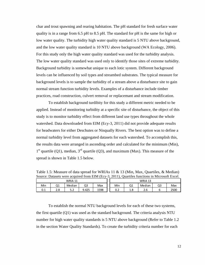
the results data were arranged in ascending order and calculated for the minimum (Min),

1st quartile (Q1), median, 3rd quartile (Q3), and maximum (Max). This measure of the

spread is shown in Table 1.5 below.

Table 1.5: Measure of data spread for WRIAs 11 & 13 (Min, Max, Quartiles, & Median) Source: Datasets were acquired from EIM (Ecy-3, 2011), Quartiles functions in Microsoft Excel.

Min Q1 Median Q3 Max Min Q1 Median Q3 Max0.1 2.8 5.2 9.425 1598 0.2 1.8 2.6 6 2500

WRIA 11 WRIA 13

To establish the normal NTU background levels for each of these two systems,

the first quartile (Q1) was used as the standard background. The criteria analysis NTU

number for high water quality standards is 5 NTU above background (Refer to Table 1.2

in the section Water Quality Standards). To create the turbidity criteria number for each

13

watershed, the following defined formula was used: Q1 plus 5 NTU equals Criteria NTU.

Q1 for WRIA 11 is 2.8 NTU and Q1 for WRIA 13 is 1.8 NTU. The formulas are:

WRIA 11: Background of 2.8 NTU (Q1) + 5 NTU = 7.8 NTU.

WRIA 13: Background of 1.8 NTU (Q1) + 5 NTU = 6.8 NTU.

Therefore the turbidity criteria are 7.8 NTU for WRIA 11 and 6.8 NTU for WRIA 13.

These adjusted water quality standards were applied as criteria to their respective

watershed turbidity datasets for analysis.

The final water quality parameter for analysis was to segregate stream (lotic) and

lake (lentic) temperature data, with stream water temperature being the primary study

objective and lake water temperature secondary for analysis. Lentic temperatures were

included in the analysis when the lotic sample site temperatures had a high frequency of

not meeting the analysis criteria. Unlike the other water quality parameters, the

temperature criteria were not based on the high and low water quality standards, but

rather on seasonal use by salmonid species. For a summary of seasonal use, refer to

Table 1.3 in the section on Water Quality Standards. Data were sorted into four

categories by seasonal use and the temperature criteria established for each of those

seasonal use categories. As with the other water quality parameters, algorithms were

created for each site and category to organize the information from blocks of site and the

seasonal specific datasets. Three information (INFO) fields were added to the seasonal

temperature algorithms before export to GIS join tables. This information was necessary to

add context for each of the seasonal tables when the information was accessed in GIS. The

new fields were: Category, Temp Criteria and Sample Period. The Category field holds

information on species, the Temp Criteria field holds the temperature analysis criteria in

degrees centigrade and the Sample Period field holds information on the month and day

range of samples taken.

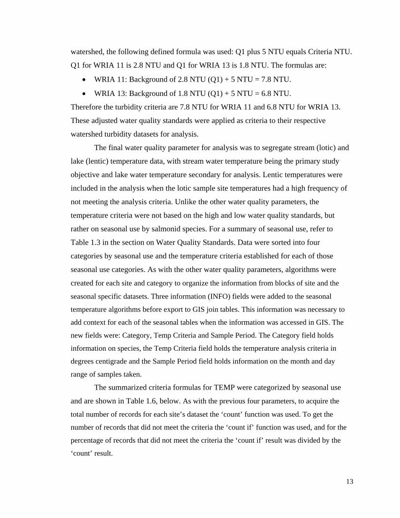
The summarized criteria formulas for TEMP were categorized by seasonal use

and are shown in Table 1.6, below. As with the previous four parameters, to acquire the

total number of records for each site’s dataset the ‘count’ function was used. To get the

number of records that did not meet the criteria the ‘count if’ function was used, and for the

percentage of records that did not meet the criteria the ‘count if’ result was divided by the

‘count’ result.

14

Table 1.6: Info, Criteria, Functions and Formulas for Seasonal Use Temperature Analysis. Source: WA water quality standards 173-201A WAC (WA Ecology, 2006) and Green, Loft and Lehr, 2009. Formulas in MS Excel.

A B C D E FField Name Function Temp 1 Temp 2 Temp 3 Temp 4

Category Text Char RearingFall/Winter/Spring Salmon & Trout

Core Summer Salmonid Habitat

Fall Char Spawning

Temp_Criteria Text 12 deg. C 13 deg. C 16 deg. C 9 deg. CSample_Period Text All_Year Sept. 16th-June 14th June 15th-Sept. 15th Sept. 16th-Dec. 22nd

1 Records COUNT [Range] [Range] [Range] [Range]2 Criteria COUNTIF [Range] > 12 deg. C [Range] > 13 deg. C [Range] > 16 deg. C [Range] > 9 deg. C3 Percent Rank DIVIDE C2 / C1 D2 / D1 E2 / E1 F2 / F1

INFO

TEMPERATURE FORMULAS

Before data could be used in the GIS portion of this analysis, a minimum number

of records (per study sample site) was needed so that the ranking of results output would

not be skewed. The Percent Rank field in each join table was used for tier ranking the

GIS display symbology. Tier ranking is explained in more detail in the next section. For

the GIS image output, the tier ranking was divided into five tiers to display the

percentage range of records not meeting the analysis criteria. For this study, sample sites

containing fewer than 5 records were discarded from the analysis.

The parameter formula and functions described above in Table 1.4 for DO, FC,

pH, and Turbidity (TURB), and Table 1.6 for Temperature (TEMP) yielded a list which

ranked each parameter by the percentage of times that study sample sites did not meet the

analysis criteria for water quality standards. Each site was given a percentile rank ranging

from zero to 100%. These percentiles were divided into a five tier ranking to define the

quality of water at a given site. The ranking was in percentile degrees from excellent to

degraded water quality. Based on the percentage of times a study sample site did not meet

the analysis criteria, the tier ranking is as follows:

Excellent (0 to 5%),

Good (>5 to 15%),

Fair (>15 to 25%),

Poor (>25 to 35%)

Degraded (>35 to 100%).

This tier ranking method was previously used in a report to analyze the water quality in

the Chehalis River Basin in Western Washington (Green et al., 2009). The procedure in

15

this study takes the analysis process several steps further than the aforementioned report.

The objective of this study was to identify the more degraded sample sites, and define

possible contributing factors from land use and impervious surfaces. This chapter deals

with the identification of degraded sites and Chapter 2 will analyze the land use and

impervious surface contributing factors. To further refine this analysis of degraded sites

two more steps were added.

After the percentile ranking of sites and dividing the list of percentile results into

five tiers, the range for the degraded water quality was selected by keeping only those

sites that rank from greater than 35% to 100% of the time not meeting the analysis

criteria. The next step used the geometric mean as a qualifier for the most degraded water

quality at sample sites. Of the sites ranking greater than 35% to 100% that did not meet

the analysis criteria, not all sites were severely degraded. For example, a site that had a

rank of 42.86% for fecal coliform (FC), with an analysis criteria of 50 CFU, could have a

minimum number of 8 CFU and a maximum number of 260 CFU, yet still have a

geometric mean of 45.37 CFU which is lower than the analysis criteria. This would be a

parameter dataset with prevailing result numbers low enough to average less than the

criteria of 50 CFU. Furthermore, a site that has the same rank of 42.86% with a minimum

number of 6 CFU and a maximum of 270 CFU can have a geometric mean of 57.35 CFU

which is higher than the analysis criteria. This would be from the dataset with numbers

that trended higher, thus giving a geometric mean result higher than the analysis criteria

of 50 CFU.

To simplify the above analysis process for finding the most degraded study

sample sites, I started with sites that had a tier rank of 35% and greater. Of those study

sample sites, only the records that had geometric means that also meet the parameter

analysis criteria (50 NTU) were selected for the final parameter ranking analysis tables.

For the FC example, all records in that group with a geometric mean of 50 CFU and

above were selected. Although some of the other parameter ranking records did not meet

the geometric mean standard, they were still included for various reasons. Explanations

will be included in the table description. The resulting tables provide lists of sites that

16

will undergo further analysis for land use and impervious surfaces. These tables are

shown in the section on Results and Conclusions in Chapter Two.

Aggregation of Ranking Results:

The methods described above created sample site ranking tables for the individual

parameters (DO, FC, pH, TURB and TEMP) in each of the watersheds within this study.

The individual tables do not allow for criteria failures across multiple parameters. The

final step in identifying the most degraded sites for water quality was to aggregate the

tables for all the parameters and rank each sample site across all parameters not meeting

the criteria at least 35% of the time. This also establishes a possible correlation between

parameters. For example, a lotic site that shows a high frequency of dissolved oxygen and

temperatures failing to meet the analysis criteria might indicate that high temperatures

could account for the low dissolved oxygen results. Thus, the aggregated tables could

provide a more refined depiction of the possible causes of degraded water quality at a

given site.

The ranking results aggregation tables were produced from the 35% parameter

ranking and geometric mean standard, exceptions included, from all the sample sites in

WRIA 11 and WRIA 13. These sample sites were in a variety of habitats including

streams, creeks and rivers (lotic), and lakes, ponds and reservoirs (lentic), and included

sample site locations at tide gates in WRIA 11. Because the primary purpose of this study

was to identify degraded lotic sites, the sample sites were stratified into three groups;

lotic, lentic, and tide gates. The lentic group was set apart as an independent variable that

could have a possible influence on water quality. Tide gates are typically located at or

near the mouth of a creek or stream where tidal influence is present. That places tide

gates at the end of a lotic system as it merges with an estuary. In this study the tide gates

were treated as an independent variable to lotic system water quality.

The above mentioned water quality data analysis process revealed some

interesting observations about water quality for both lentic systems and tide gates, as well

as the intended analysis for lotic systems. These findings will be discussed in detail in the

Results and Conclusions section in Chapter Two. The tables created for the lotic system

17

ranking analysis and the aggregation of ranking result tables are joined to GIS features to

graphically represent the data.

GIS Spatial Data and Join Tables:

Spatial data is information that has a reference to a geographic coordinate. This

information is used to create features on a map like points, lines and polygons that

represent features in the real world. These features can contain information about the

feature like ID, location, shape, length and area. These are stored in a geographic

information system (GIS) in a tabular form. These attribute tables in GIS can be

expanded by providing more information to the system. A whole database of information

can be created by adding fields within the GIS software to populate the attribute tables

with more feature data.

Another way to populate GIS attribute tables is by the use of joins or relates. The

GIS join tables are external tabular data appended to the feature attribute table by a

common field. The appended data becomes a permanent part of the feature attribute table

as long as the join is not removed. Relate tables work similarly to join tables in that they

need a common field to provide information to the feature attribute table. The difference

is that relate tables are a lookup source of information and are not appended to the feature

attribute table.

For this study, the data came from the Washington Department of Ecology’s EIM

database (Ecy-3, 2011). From the data extracted for WRIA11 and WRIA 13, two tables

were created externally from GIS, in Microsoft Excel. One table was used for location

information and to generate GIS spatial features for the water quality monitoring sites.

The other table was made up of the sample results and was used for the tabular data

analysis. When both steps were completed, the analysis results table was joined to the

GIS location feature data so spatial analysis on the sampling sties could be performed.

The external tables had two primary functions for this study. First, to show the location of

sample study sites analyzed and second, to provide a colored tier ranking for the percentage

of time the data set did not meet the criteria for each of the parameters. The tables for the

aggregation of ranking results were used to create a set of GIS features to graphically

represent those sites that were the most degraded across multiple parameters. Some of the

18

features created for the most degraded sites were used as end points for defining flow basins

and to calculate area of influence from land use. The spatial analysis for flow basins and land

use is explained in Chapter Four.

19

Chapter Two:

Identification of Degraded Habitat in Lotic Freshwater Systems

Results and Conclusions:

The following tables, in the section on Results for WRIA 11, show the results of

analysis performed on water quality data for Dissolved Oxygen (DO), Fecal Coliform

(FC), Turbidity (TURB) and Temperature (TEMP) in the Nisqually Basin (WRIA 11).

For the pH parameter in WRIA 11, none of the study sample sites had a percentile rank

above 35%. The following tables, in the section on Results for WRIA 13, show the

results of analysis for Dissolved Oxygen (DO), Fecal Coliform (FC), pH, Turbidity

(TURB) and Temperature (TEMP) in the Deschutes Basin (WRIA 13). The TEMP data

were subject to a different criteria method than the other parameters. The analysis criteria

for DO, FC, pH and TURB were based on the high and low water quality standards (See

Table 1.2) and the criteria for TEMP were based on seasonal temperature requirements

for salmonids (See Table 1.3). The results in the tables below were derived from a series

of criteria designed to cull out sample sites showing degraded water quality. The first step

defined the percentage of times the study site samples failed to meet the criteria

established for each parameter. Those results were organized in descending order by

percent. The second step took all records that had a percentile criteria failure equal to or

greater than 35% of the samples with the geometric mean of that dataset also not meeting

each parameter’s criteria. Example 1: Criteria = FC > 50 cfu. Records > 50 cfu = 50%

and Geometric Mean = 66.99. Both are greater than the criteria. This is referred to as

the 35% plus geometric mean standard. A few records equal to or above 35% and where

the geometric mean did meet the parameter analysis criteria were kept in this list for

various reasons. Example 2: Criteria = FC > 50 cfu. Records > 50 cfu = 50% and

Geometric Mean = 27.31. Geometric Mean not greater than the criteria. These records

were considered sites of interest and will be explained for each parameter where they

occur. Usually analysis records like the second example were due to high intermittent

failures to meet the criteria.

20

Results for WRIA 11:

The following tables were used in the Nisqually Basin analysis study. The tables

in this section show results from the series parameter analysis criteria to establish those

sites that show the highest potential for degraded aquatic habitat.

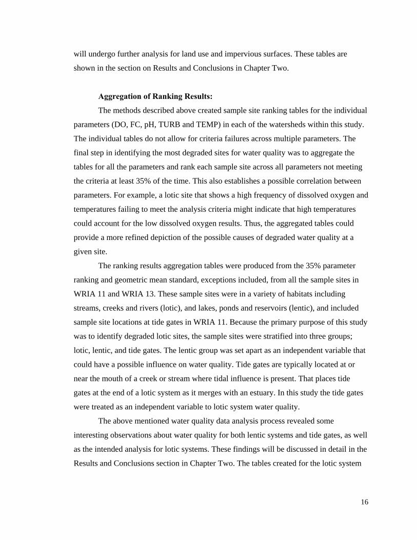
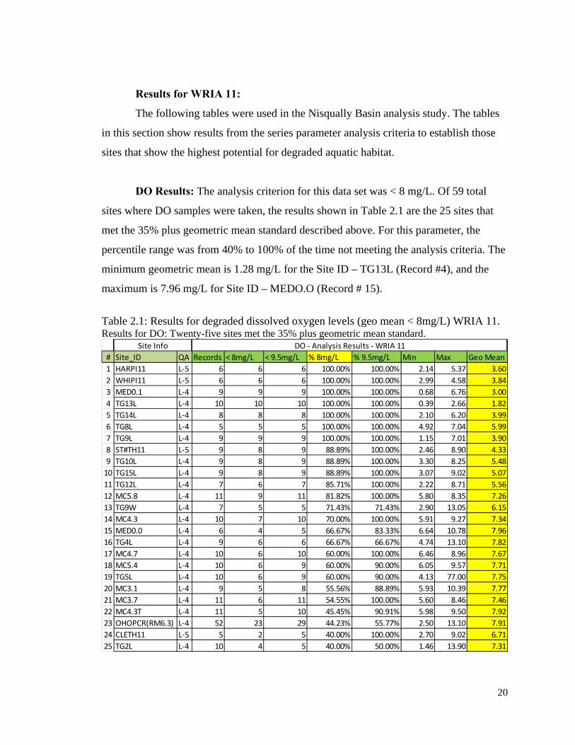
DO Results: The analysis criterion for this data set was < 8 mg/L. Of 59 total

sites where DO samples were taken, the results shown in Table 2.1 are the 25 sites that

met the 35% plus geometric mean standard described above. For this parameter, the

percentile range was from 40% to 100% of the time not meeting the analysis criteria. The

minimum geometric mean is 1.28 mg/L for the Site ID – TG13L (Record #4), and the

maximum is 7.96 mg/L for Site ID – MEDO.O (Record # 15).

Table 2.1: Results for degraded dissolved oxygen levels (geo mean < 8mg/L) WRIA 11. Results for DO: Twenty-five sites met the 35% plus geometric mean standard.

# Site_ID QA Records < 8mg/L < 9.5mg/L % 8mg/L % 9.5mg/L Min Max Geo Mean1 HARPI11 L-5 6 6 6 100.00% 100.00% 2.14 5.37 3.602 WHIPI11 L-5 6 6 6 100.00% 100.00% 2.99 4.58 3.843 MED0.1 L-4 9 9 9 100.00% 100.00% 0.68 6.76 3.004 TG13L L-4 10 10 10 100.00% 100.00% 0.39 2.66 1.825 TG14L L-4 8 8 8 100.00% 100.00% 2.10 6.20 3.996 TG8L L-4 5 5 5 100.00% 100.00% 4.92 7.04 5.997 TG9L L-4 9 9 9 100.00% 100.00% 1.15 7.01 3.908 ST#TH11 L-5 9 8 9 88.89% 100.00% 2.46 8.90 4.339 TG10L L-4 9 8 9 88.89% 100.00% 3.30 8.25 5.48

10 TG15L L-4 9 8 9 88.89% 100.00% 3.07 9.02 5.0711 TG12L L-4 7 6 7 85.71% 100.00% 2.22 8.71 5.5612 MC5.8 L-4 11 9 11 81.82% 100.00% 5.80 8.35 7.2613 TG9W L-4 7 5 5 71.43% 71.43% 2.90 13.05 6.1514 MC4.3 L-4 10 7 10 70.00% 100.00% 5.91 9.27 7.3415 MED0.0 L-4 6 4 5 66.67% 83.33% 6.64 10.78 7.9616 TG4L L-4 9 6 6 66.67% 66.67% 4.74 13.10 7.8217 MC4.7 L-4 10 6 10 60.00% 100.00% 6.46 8.96 7.6718 MC5.4 L-4 10 6 9 60.00% 90.00% 6.05 9.57 7.7119 TG5L L-4 10 6 9 60.00% 90.00% 4.13 77.00 7.7520 MC3.1 L-4 9 5 8 55.56% 88.89% 5.93 10.39 7.7721 MC3.7 L-4 11 6 11 54.55% 100.00% 5.60 8.46 7.4622 MC4.3T L-4 11 5 10 45.45% 90.91% 5.98 9.50 7.9223 OHOPCR(RM6.3) L-4 52 23 29 44.23% 55.77% 2.50 13.10 7.9124 CLETH11 L-5 5 2 5 40.00% 100.00% 2.70 9.02 6.7125 TG2L L-4 10 4 5 40.00% 50.00% 1.46 13.90 7.31

Site Info DO - Analysis Results - WRIA 11

21

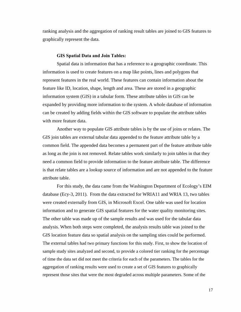
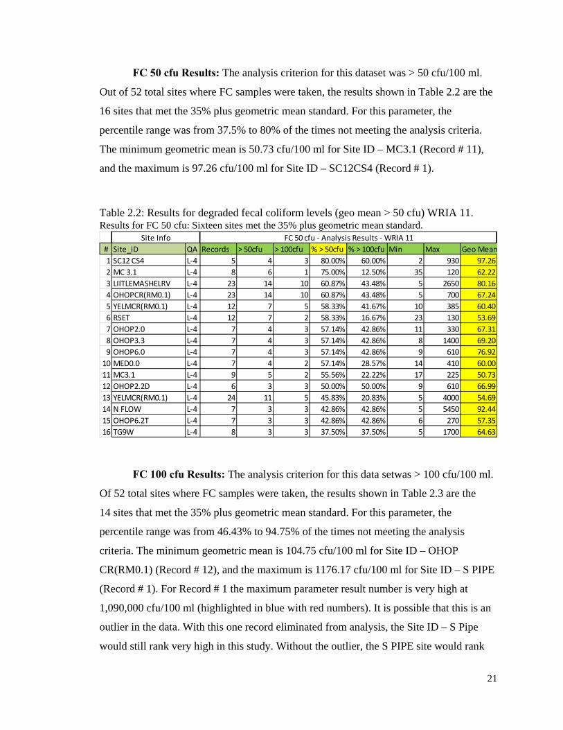
FC 50 cfu Results: The analysis criterion for this dataset was > 50 cfu/100 ml.

Out of 52 total sites where FC samples were taken, the results shown in Table 2.2 are the

16 sites that met the 35% plus geometric mean standard. For this parameter, the

percentile range was from 37.5% to 80% of the times not meeting the analysis criteria.

The minimum geometric mean is 50.73 cfu/100 ml for Site ID – MC3.1 (Record # 11),

and the maximum is 97.26 cfu/100 ml for Site ID – SC12CS4 (Record # 1).

Table 2.2: Results for degraded fecal coliform levels (geo mean > 50 cfu) WRIA 11. Results for FC 50 cfu: Sixteen sites met the 35% plus geometric mean standard.

# Site_ID QA Records > 50cfu > 100cfu % > 50cfu % > 100cfu Min Max Geo Mean1 SC12 CS4 L-4 5 4 3 80.00% 60.00% 2 930 97.262 MC 3.1 L-4 8 6 1 75.00% 12.50% 35 120 62.223 LIITLEMASHELRV L-4 23 14 10 60.87% 43.48% 5 2650 80.164 OHOPCR(RM0.1) L-4 23 14 10 60.87% 43.48% 5 700 67.245 YELMCR(RM0.1) L-4 12 7 5 58.33% 41.67% 10 385 60.406 RSET L-4 12 7 2 58.33% 16.67% 23 130 53.697 OHOP2.0 L-4 7 4 3 57.14% 42.86% 11 330 67.318 OHOP3.3 L-4 7 4 3 57.14% 42.86% 8 1400 69.209 OHOP6.0 L-4 7 4 3 57.14% 42.86% 9 610 76.92

10 MED0.0 L-4 7 4 2 57.14% 28.57% 14 410 60.0011 MC3.1 L-4 9 5 2 55.56% 22.22% 17 225 50.7312 OHOP2.2D L-4 6 3 3 50.00% 50.00% 9 610 66.9913 YELMCR(RM0.1) L-4 24 11 5 45.83% 20.83% 5 4000 54.6914 N FLOW L-4 7 3 3 42.86% 42.86% 5 5450 92.4415 OHOP6.2T L-4 7 3 3 42.86% 42.86% 6 270 57.3516 TG9W L-4 8 3 3 37.50% 37.50% 5 1700 64.63

Site Info FC 50 cfu - Analysis Results - WRIA 11

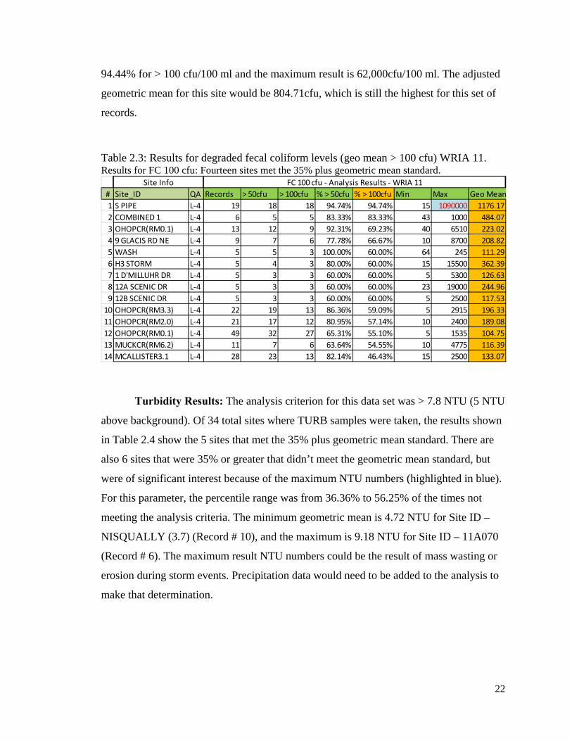
FC 100 cfu Results: The analysis criterion for this data setwas > 100 cfu/100 ml.

Of 52 total sites where FC samples were taken, the results shown in Table 2.3 are the

14 sites that met the 35% plus geometric mean standard. For this parameter, the

percentile range was from 46.43% to 94.75% of the times not meeting the analysis

criteria. The minimum geometric mean is 104.75 cfu/100 ml for Site ID – OHOP

CR(RM0.1) (Record # 12), and the maximum is 1176.17 cfu/100 ml for Site ID – S PIPE

(Record # 1). For Record # 1 the maximum parameter result number is very high at

1,090,000 cfu/100 ml (highlighted in blue with red numbers). It is possible that this is an

outlier in the data. With this one record eliminated from analysis, the Site ID – S Pipe

would still rank very high in this study. Without the outlier, the S PIPE site would rank

22

94.44% for > 100 cfu/100 ml and the maximum result is 62,000cfu/100 ml. The adjusted

geometric mean for this site would be 804.71cfu, which is still the highest for this set of

records.

Table 2.3: Results for degraded fecal coliform levels (geo mean > 100 cfu) WRIA 11. Results for FC 100 cfu: Fourteen sites met the 35% plus geometric mean standard.

# Site_ID QA Records > 50cfu > 100cfu % > 50cfu % > 100cfu Min Max Geo Mean1 S PIPE L-4 19 18 18 94.74% 94.74% 15 1090000 1176.172 COMBINED 1 L-4 6 5 5 83.33% 83.33% 43 1000 484.073 OHOPCR(RM0.1) L-4 13 12 9 92.31% 69.23% 40 6510 223.024 9 GLACIS RD NE L-4 9 7 6 77.78% 66.67% 10 8700 208.825 WASH L-4 5 5 3 100.00% 60.00% 64 245 111.296 H3 STORM L-4 5 4 3 80.00% 60.00% 15 15500 362.397 1 D'MILLUHR DR L-4 5 3 3 60.00% 60.00% 5 5300 126.638 12A SCENIC DR L-4 5 3 3 60.00% 60.00% 23 19000 244.969 12B SCENIC DR L-4 5 3 3 60.00% 60.00% 5 2500 117.53

10 OHOPCR(RM3.3) L-4 22 19 13 86.36% 59.09% 5 2915 196.3311 OHOPCR(RM2.0) L-4 21 17 12 80.95% 57.14% 10 2400 189.0812 OHOPCR(RM0.1) L-4 49 32 27 65.31% 55.10% 5 1535 104.7513 MUCKCR(RM6.2) L-4 11 7 6 63.64% 54.55% 10 4775 116.3914 MCALLISTER3.1 L-4 28 23 13 82.14% 46.43% 15 2500 133.07

Site Info FC 100 cfu - Analysis Results - WRIA 11

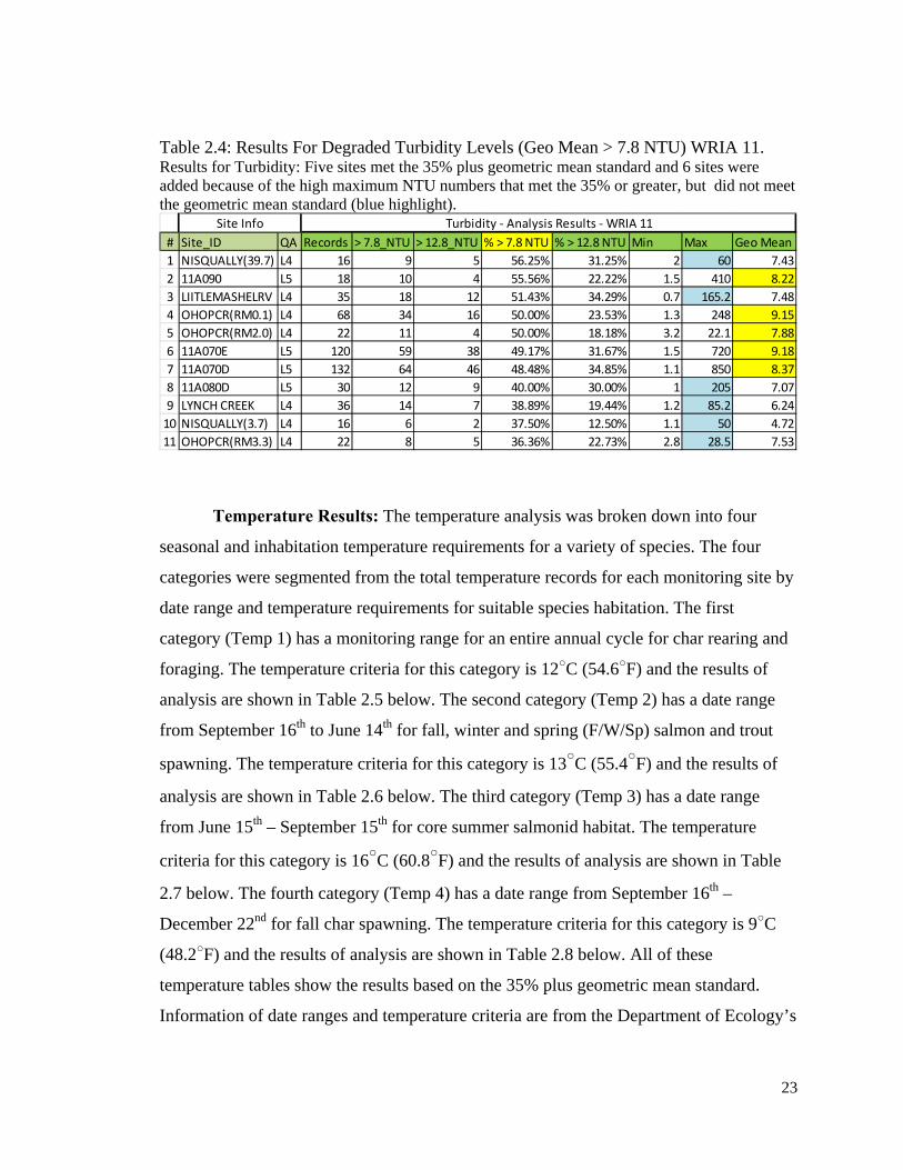
Turbidity Results: The analysis criterion for this data set was > 7.8 NTU (5 NTU

above background). Of 34 total sites where TURB samples were taken, the results shown

in Table 2.4 show the 5 sites that met the 35% plus geometric mean standard. There are

also 6 sites that were 35% or greater that didn’t meet the geometric mean standard, but

were of significant interest because of the maximum NTU numbers (highlighted in blue).

For this parameter, the percentile range was from 36.36% to 56.25% of the times not

meeting the analysis criteria. The minimum geometric mean is 4.72 NTU for Site ID –

NISQUALLY (3.7) (Record # 10), and the maximum is 9.18 NTU for Site ID – 11A070

(Record # 6). The maximum result NTU numbers could be the result of mass wasting or

erosion during storm events. Precipitation data would need to be added to the analysis to

make that determination.

23

Table 2.4: Results For Degraded Turbidity Levels (Geo Mean > 7.8 NTU) WRIA 11. Results for Turbidity: Five sites met the 35% plus geometric mean standard and 6 sites were added because of the high maximum NTU numbers that met the 35% or greater, but did not meet the geometric mean standard (blue highlight).

# Site_ID QA Records > 7.8_NTU > 12.8_NTU % > 7.8 NTU % > 12.8 NTU Min Max Geo Mean1 NISQUALLY(39.7) L4 16 9 5 56.25% 31.25% 2 60 7.432 11A090 L5 18 10 4 55.56% 22.22% 1.5 410 8.223 LIITLEMASHELRV L4 35 18 12 51.43% 34.29% 0.7 165.2 7.484 OHOPCR(RM0.1) L4 68 34 16 50.00% 23.53% 1.3 248 9.155 OHOPCR(RM2.0) L4 22 11 4 50.00% 18.18% 3.2 22.1 7.886 11A070E L5 120 59 38 49.17% 31.67% 1.5 720 9.187 11A070D L5 132 64 46 48.48% 34.85% 1.1 850 8.378 11A080D L5 30 12 9 40.00% 30.00% 1 205 7.079 LYNCH CREEK L4 36 14 7 38.89% 19.44% 1.2 85.2 6.24

10 NISQUALLY(3.7) L4 16 6 2 37.50% 12.50% 1.1 50 4.7211 OHOPCR(RM3.3) L4 22 8 5 36.36% 22.73% 2.8 28.5 7.53

Site Info Turbidity - Analysis Results - WRIA 11

Temperature Results: The temperature analysis was broken down into four

seasonal and inhabitation temperature requirements for a variety of species. The four

categories were segmented from the total temperature records for each monitoring site by

date range and temperature requirements for suitable species habitation. The first

category (Temp 1) has a monitoring range for an entire annual cycle for char rearing and

foraging. The temperature criteria for this category is 12○C (54.6○F) and the results of

analysis are shown in Table 2.5 below. The second category (Temp 2) has a date range

from September 16th to June 14th for fall, winter and spring (F/W/Sp) salmon and trout

spawning. The temperature criteria for this category is 13○C (55.4○F) and the results of

analysis are shown in Table 2.6 below. The third category (Temp 3) has a date range

from June 15th – September 15th for core summer salmonid habitat. The temperature

criteria for this category is 16○C (60.8○F) and the results of analysis are shown in Table

2.7 below. The fourth category (Temp 4) has a date range from September 16th –

December 22nd for fall char spawning. The temperature criteria for this category is 9○C

(48.2○F) and the results of analysis are shown in Table 2.8 below. All of these

temperature tables show the results based on the 35% plus geometric mean standard.

Information of date ranges and temperature criteria are from the Department of Ecology’s

24

Water Quality Standards for Surface Water of the State of Washington, Chapter 173-

201A WAC (WA Ecology, 2006).

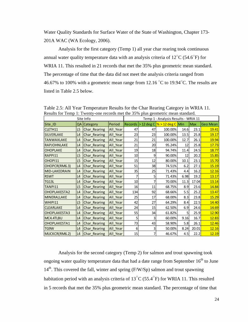
Analysis for the first category (Temp 1) all year char rearing took continuous

annual water quality temperature data with an analysis criteria of 12○C (54.6○F) for

WRIA 11. This resulted in 21 records that met the 35% plus geometric mean standard.

The percentage of time that the data did not meet the analysis criteria ranged from

46.67% to 100% with a geometric mean range from 12.16 ○C to 19.94○C. The results are

listed in Table 2.5 below.

Table 2.5: All Year Temperature Results for the Char Rearing Category in WRIA 11. Results for Temp 1: Twenty-one records met the 35% plus geometric mean standard.

Site_ID QA Category Period Records > 12 deg C % > 12 deg C Min Max Geo MeanCLETH11 L5 Char_Rearing All_Year 47 47 100.00% 14.6 23.1 19.41SILVERLAKE L4 Char_Rearing All_Year 23 23 100.00% 13.5 25.8 19.17TANWAXLAKE L4 Char_Rearing All_Year 21 21 100.00% 12.7 26.1 19.94RAPJOHNLAKE L4 Char_Rearing All_Year 21 20 95.24% 12 25.8 17.73OHOPLAKE L4 Char_Rearing All_Year 19 18 94.74% 11.4 24.5 18.77RAPPI11 L5 Char_Rearing All_Year 10 9 90.00% 12 20.2 15.85OHOPI11 L5 Char_Rearing All_Year 15 12 80.00% 10.1 23.1 15.70OHOPCR(RM6.3) L4 Char_Rearing All_Year 51 38 74.51% 6.2 27.1 15.19MID-LAKEDRAIN L4 Char_Rearing All_Year 35 25 71.43% 4.4 16.2 12.16RSWT L4 Char_Rearing All_Year 7 5 71.43% 6.98 19.2 13.17TG13L L4 Char_Rearing All_Year 10 7 70.00% 11.3 17.04 13.14TANPI11 L5 Char_Rearing All_Year 16 11 68.75% 8.9 23.6 14.84OHOPLAKESTA2 L4 Char_Rearing All_Year 134 92 68.66% 5.5 25.2 13.47MINERALLAKE L4 Char_Rearing All_Year 25 17 68.00% 8.3 23.8 15.29WHIPI11 L5 Char_Rearing All_Year 42 27 64.29% 8.4 22.5 14.40CLEARLAKE L4 Char_Rearing All_Year 24 15 62.50% 6.9 24.6 14.69OHOPLAKESTA3 L4 Char_Rearing All_Year 55 34 61.82% 5 25.9 12.90MC4.4TLBU L4 Char_Rearing All_Year 5 3 60.00% 9.16 16.7 12.83OHOPLAKESTA1 L4 Char_Rearing All_Year 73 43 58.90% 5.8 26.1 12.46TG9W L4 Char_Rearing All_Year 6 3 50.00% 8.24 20.01 12.16MUCKCR(RM6.2) L4 Char_Rearing All_Year 15 7 46.67% 4.5 22.2 12.19

Site Info Temp 1 - Analysis Results - WRIA 11

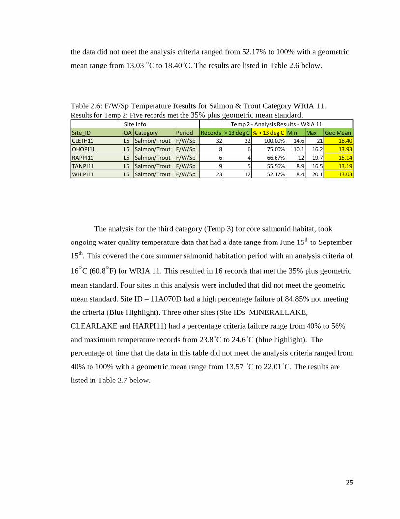
Analysis for the second category (Temp 2) for salmon and trout spawning took

ongoing water quality temperature data that had a date range from September 16th to June

14th. This covered the fall, winter and spring (F/W/Sp) salmon and trout spawning

habitation period with an analysis criteria of 13○C (55.4○F) for WRIA 11. This resulted

in 5 records that met the 35% plus geometric mean standard. The percentage of time that

25

the data did not meet the analysis criteria ranged from 52.17% to 100% with a geometric

mean range from 13.03 ○C to 18.40○C. The results are listed in Table 2.6 below.

Table 2.6: F/W/Sp Temperature Results for Salmon & Trout Category WRIA 11. Results for Temp 2: Five records met the 35% plus geometric mean standard.

Site_ID QA Category Period Records > 13 deg C % > 13 deg C Min Max Geo MeanCLETH11 L5 Salmon/Trout F/W/Sp 32 32 100.00% 14.6 21 18.40OHOPI11 L5 Salmon/Trout F/W/Sp 8 6 75.00% 10.1 16.2 13.93RAPPI11 L5 Salmon/Trout F/W/Sp 6 4 66.67% 12 19.7 15.14TANPI11 L5 Salmon/Trout F/W/Sp 9 5 55.56% 8.9 16.5 13.19WHIPI11 L5 Salmon/Trout F/W/Sp 23 12 52.17% 8.4 20.1 13.03


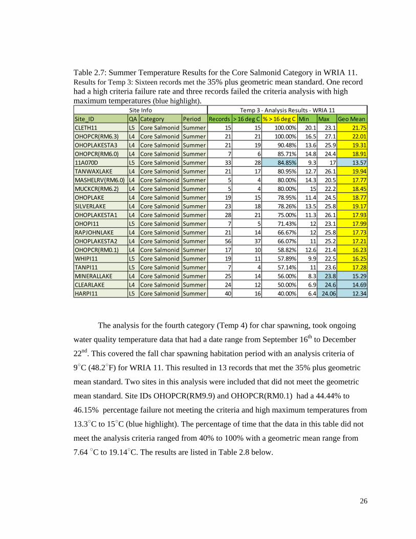
The analysis for the third category (Temp 3) for core salmonid habitat, took

ongoing water quality temperature data that had a date range from June 15th to September

15th. This covered the core summer salmonid habitation period with an analysis criteria of

16○C (60.8○F) for WRIA 11. This resulted in 16 records that met the 35% plus geometric

mean standard. Four sites in this analysis were included that did not meet the geometric

mean standard. Site ID – 11A070D had a high percentage failure of 84.85% not meeting

the criteria (Blue Highlight). Three other sites (Site IDs: MINERALLAKE,

CLEARLAKE and HARPI11) had a percentage criteria failure range from 40% to 56%

and maximum temperature records from 23.8○C to 24.6○C (blue highlight). The

percentage of time that the data in this table did not meet the analysis criteria ranged from

40% to 100% with a geometric mean range from 13.57 ○C to 22.01○C. The results are

listed in Table 2.7 below.

26

Table 2.7: Summer Temperature Results for the Core Salmonid Category in WRIA 11. Results for Temp 3: Sixteen records met the 35% plus geometric mean standard. One record had a high criteria failure rate and three records failed the criteria analysis with high maximum temperatures (blue highlight).

Site_ID QA Category Period Records > 16 deg C % > 16 deg C Min Max Geo MeanCLETH11 L5 Core Salmonid Summer 15 15 100.00% 20.1 23.1 21.75OHOPCR(RM6.3) L4 Core Salmonid Summer 21 21 100.00% 16.5 27.1 22.01OHOPLAKESTA3 L4 Core Salmonid Summer 21 19 90.48% 13.6 25.9 19.31OHOPCR(RM6.0) L4 Core Salmonid Summer 7 6 85.71% 14.8 24.4 18.9111A070D L5 Core Salmonid Summer 33 28 84.85% 9.3 17 13.57TANWAXLAKE L4 Core Salmonid Summer 21 17 80.95% 12.7 26.1 19.94MASHELRV(RM6.0) L4 Core Salmonid Summer 5 4 80.00% 14.3 20.5 17.77MUCKCR(RM6.2) L4 Core Salmonid Summer 5 4 80.00% 15 22.2 18.45OHOPLAKE L4 Core Salmonid Summer 19 15 78.95% 11.4 24.5 18.77SILVERLAKE L4 Core Salmonid Summer 23 18 78.26% 13.5 25.8 19.17OHOPLAKESTA1 L4 Core Salmonid Summer 28 21 75.00% 11.3 26.1 17.93OHOPI11 L5 Core Salmonid Summer 7 5 71.43% 12 23.1 17.99RAPJOHNLAKE L4 Core Salmonid Summer 21 14 66.67% 12 25.8 17.73OHOPLAKESTA2 L4 Core Salmonid Summer 56 37 66.07% 11 25.2 17.21OHOPCR(RM0.1) L4 Core Salmonid Summer 17 10 58.82% 12.6 21.4 16.23WHIPI11 L5 Core Salmonid Summer 19 11 57.89% 9.9 22.5 16.25TANPI11 L5 Core Salmonid Summer 7 4 57.14% 11 23.6 17.28MINERALLAKE L4 Core Salmonid Summer 25 14 56.00% 8.3 23.8 15.29CLEARLAKE L4 Core Salmonid Summer 24 12 50.00% 6.9 24.6 14.69HARPI11 L5 Core Salmonid Summer 40 16 40.00% 6.4 24.06 12.34


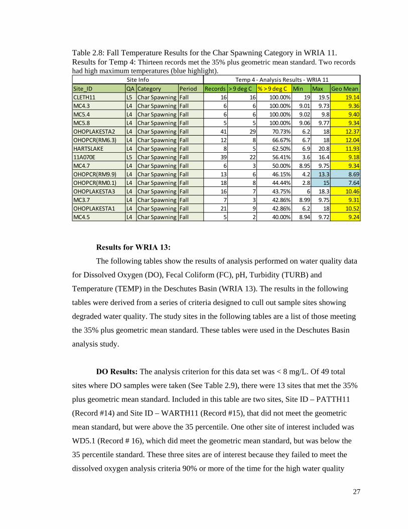
The analysis for the fourth category (Temp 4) for char spawning, took ongoing

water quality temperature data that had a date range from September 16th to December

22nd. This covered the fall char spawning habitation period with an analysis criteria of

9○C (48.2○F) for WRIA 11. This resulted in 13 records that met the 35% plus geometric

mean standard. Two sites in this analysis were included that did not meet the geometric

mean standard. Site IDs OHOPCR(RM9.9) and OHOPCR(RM0.1) had a 44.44% to

46.15% percentage failure not meeting the criteria and high maximum temperatures from

13.3○C to 15○C (blue highlight). The percentage of time that the data in this table did not

meet the analysis criteria ranged from 40% to 100% with a geometric mean range from

7.64 ○C to 19.14○C. The results are listed in Table 2.8 below.

27

Table 2.8: Fall Temperature Results for the Char Spawning Category in WRIA 11. Results for Temp 4: Thirteen records met the 35% plus geometric mean standard. Two records had high maximum temperatures (blue highlight).

Site_ID QA Category Period Records > 9 deg C % > 9 deg C Min Max Geo MeanCLETH11 L5 Char Spawning Fall 16 16 100.00% 19 19.5 19.14MC4.3 L4 Char Spawning Fall 6 6 100.00% 9.01 9.73 9.36MC5.4 L4 Char Spawning Fall 6 6 100.00% 9.02 9.8 9.40MC5.8 L4 Char Spawning Fall 5 5 100.00% 9.06 9.77 9.34OHOPLAKESTA2 L4 Char Spawning Fall 41 29 70.73% 6.2 18 12.37OHOPCR(RM6.3) L4 Char Spawning Fall 12 8 66.67% 6.7 18 12.04HARTSLAKE L4 Char Spawning Fall 8 5 62.50% 6.9 20.8 11.9311A070E L5 Char Spawning Fall 39 22 56.41% 3.6 16.4 9.18MC4.7 L4 Char Spawning Fall 6 3 50.00% 8.95 9.75 9.34OHOPCR(RM9.9) L4 Char Spawning Fall 13 6 46.15% 4.2 13.3 8.69OHOPCR(RM0.1) L4 Char Spawning Fall 18 8 44.44% 2.8 15 7.64OHOPLAKESTA3 L4 Char Spawning Fall 16 7 43.75% 6 18.3 10.46MC3.7 L4 Char Spawning Fall 7 3 42.86% 8.99 9.75 9.31OHOPLAKESTA1 L4 Char Spawning Fall 21 9 42.86% 6.2 18 10.52MC4.5 L4 Char Spawning Fall 5 2 40.00% 8.94 9.72 9.24


Results for WRIA 13:

The following tables show the results of analysis performed on water quality data

for Dissolved Oxygen (DO), Fecal Coliform (FC), pH, Turbidity (TURB) and

Temperature (TEMP) in the Deschutes Basin (WRIA 13). The results in the following

tables were derived from a series of criteria designed to cull out sample sites showing

degraded water quality. The study sites in the following tables are a list of those meeting

the 35% plus geometric mean standard. These tables were used in the Deschutes Basin

analysis study.

DO Results: The analysis criterion for this data set was < 8 mg/L. Of 49 total

sites where DO samples were taken (See Table 2.9), there were 13 sites that met the 35%

plus geometric mean standard. Included in this table are two sites, Site ID – PATTH11

(Record #14) and Site ID – WARTH11 (Record #15), that did not meet the geometric

mean standard, but were above the 35 percentile. One other site of interest included was

WD5.1 (Record # 16), which did meet the geometric mean standard, but was below the

35 percentile standard. These three sites are of interest because they failed to meet the

dissolved oxygen analysis criteria 90% or more of the time for the high water quality

28

standard of 9.5mg/L. For this parameter, the percentile range was from 25% to 100% of

the times not meeting the analysis criteria. The minimum geometric mean is 4.99 mg/L

for the Site ID – SPDITCH2 (Record #2), and the maximum is 8.24 mg/L for Site ID –

WARTH11 (Record # 15).

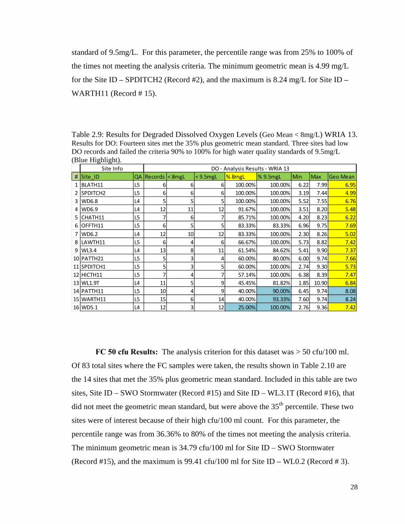
Table 2.9: Results for Degraded Dissolved Oxygen Levels (Geo Mean < 8mg/L) WRIA 13. Results for DO: Fourteen sites met the 35% plus geometric mean standard. Three sites had low DO records and failed the criteria 90% to 100% for high water quality standards of 9.5mg/L (Blue Highlight).

# Site_ID QA Records < 8mgL < 9.5mgL % 8mgL % 9.5mgL Min Max Geo Mean1 BLATH11 L5 6 6 6 100.00% 100.00% 6.22 7.99 6.952 SPDITCH2 L5 6 6 6 100.00% 100.00% 3.19 7.44 4.993 WD6.8 L4 5 5 5 100.00% 100.00% 5.52 7.55 6.764 WD6.9 L4 12 11 12 91.67% 100.00% 3.51 8.20 5.485 CHATH11 L5 7 6 7 85.71% 100.00% 4.20 8.23 6.226 OFFTH11 L5 6 5 5 83.33% 83.33% 6.96 9.75 7.697 WD6.2 L4 12 10 12 83.33% 100.00% 2.30 8.26 5.028 LAWTH11 L5 6 4 6 66.67% 100.00% 5.73 8.82 7.429 WL3.4 L4 13 8 11 61.54% 84.62% 5.41 9.90 7.37

10 PATTH21 L5 5 3 4 60.00% 80.00% 6.00 9.74 7.6611 SPDITCH1 L5 5 3 5 60.00% 100.00% 2.74 9.30 5.7312 HICTH11 L5 7 4 7 57.14% 100.00% 6.38 8.39 7.4713 WL1.9T L4 11 5 9 45.45% 81.82% 1.85 10.90 6.8414 PATTH11 L5 10 4 9 40.00% 90.00% 6.45 9.74 8.0815 WARTH11 L5 15 6 14 40.00% 93.33% 7.60 9.74 8.2416 WD5.1 L4 12 3 12 25.00% 100.00% 2.76 9.36 7.42

Site Info DO - Analysis Results - WRIA 13

FC 50 cfu Results: The analysis criterion for this dataset was > 50 cfu/100 ml.

Of 83 total sites where the FC samples were taken, the results shown in Table 2.10 are

the 14 sites that met the 35% plus geometric mean standard. Included in this table are two

sites, Site ID – SWO Stormwater (Record #15) and Site ID – WL3.1T (Record #16), that

did not meet the geometric mean standard, but were above the 35th percentile. These two

sites were of interest because of their high cfu/100 ml count. For this parameter, the


The minimum geometric mean is 34.79 cfu/100 ml for Site ID – SWO Stormwater

(Record #15), and the maximum is 99.41 cfu/100 ml for Site ID – WL0.2 (Record # 3).

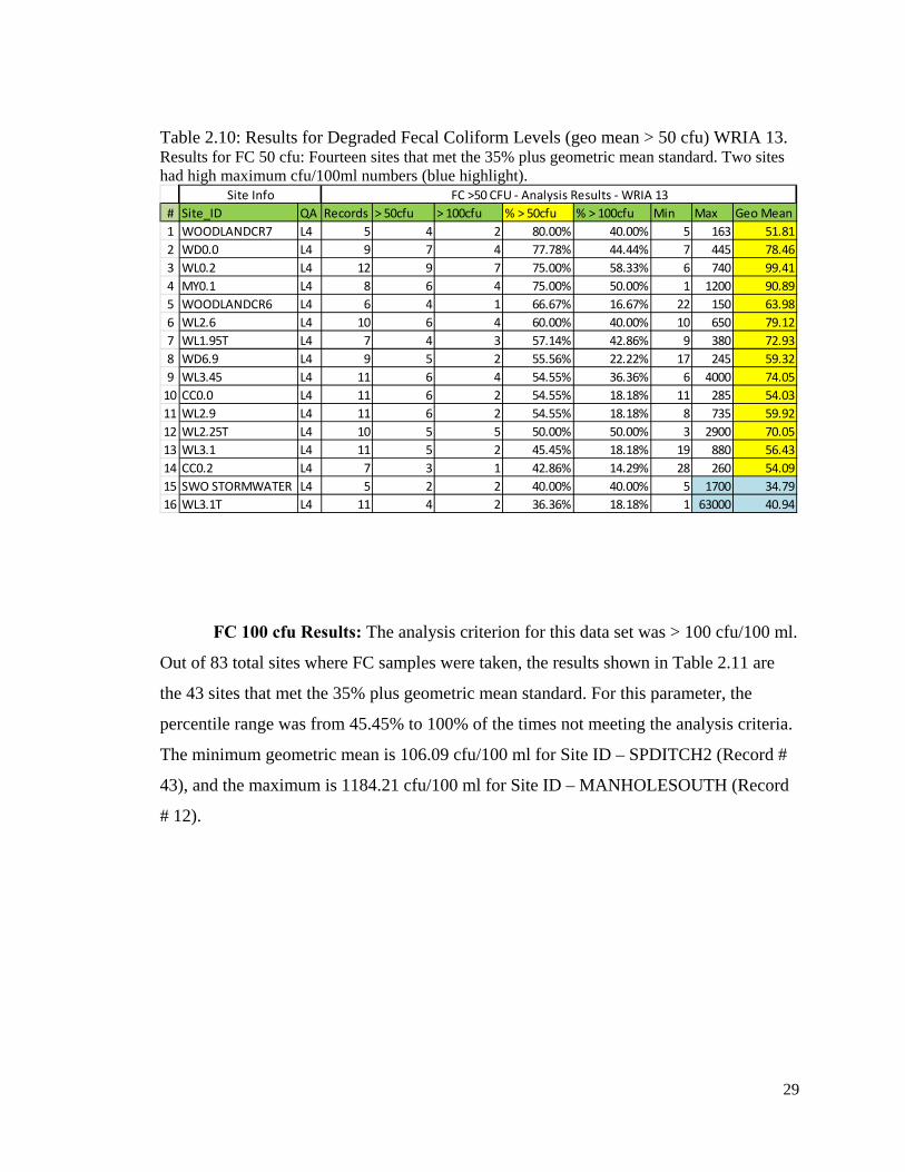
29

Table 2.10: Results for Degraded Fecal Coliform Levels (geo mean > 50 cfu) WRIA 13. Results for FC 50 cfu: Fourteen sites that met the 35% plus geometric mean standard. Two sites had high maximum cfu/100ml numbers (blue highlight).

# Site_ID QA Records > 50cfu > 100cfu % > 50cfu % > 100cfu Min Max Geo Mean1 WOODLANDCR7 L4 5 4 2 80.00% 40.00% 5 163 51.812 WD0.0 L4 9 7 4 77.78% 44.44% 7 445 78.463 WL0.2 L4 12 9 7 75.00% 58.33% 6 740 99.414 MY0.1 L4 8 6 4 75.00% 50.00% 1 1200 90.895 WOODLANDCR6 L4 6 4 1 66.67% 16.67% 22 150 63.986 WL2.6 L4 10 6 4 60.00% 40.00% 10 650 79.127 WL1.95T L4 7 4 3 57.14% 42.86% 9 380 72.938 WD6.9 L4 9 5 2 55.56% 22.22% 17 245 59.329 WL3.45 L4 11 6 4 54.55% 36.36% 6 4000 74.05

10 CC0.0 L4 11 6 2 54.55% 18.18% 11 285 54.0311 WL2.9 L4 11 6 2 54.55% 18.18% 8 735 59.9212 WL2.25T L4 10 5 5 50.00% 50.00% 3 2900 70.0513 WL3.1 L4 11 5 2 45.45% 18.18% 19 880 56.4314 CC0.2 L4 7 3 1 42.86% 14.29% 28 260 54.0915 SWO STORMWATER L4 5 2 2 40.00% 40.00% 5 1700 34.7916 WL3.1T L4 11 4 2 36.36% 18.18% 1 63000 40.94

Site Info FC >50 CFU - Analysis Results - WRIA 13

FC 100 cfu Results: The analysis criterion for this data set was > 100 cfu/100 ml.

Out of 83 total sites where FC samples were taken, the results shown in Table 2.11 are

the 43 sites that met the 35% plus geometric mean standard. For this parameter, the


The minimum geometric mean is 106.09 cfu/100 ml for Site ID – SPDITCH2 (Record #

43), and the maximum is 1184.21 cfu/100 ml for Site ID – MANHOLESOUTH (Record

# 12).

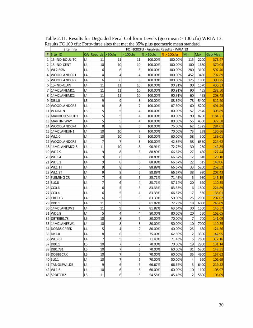
30

Table 2.11: Results for Degraded Fecal Coliform Levels (geo mean > 100 cfu) WRIA 13. Results FC 100 cfu: Forty-three sites that met the 35% plus geometric mean standard.

# Site_ID QA Records > 50cfu > 100cfu % > 50cfu % > 100cfu Min Max Geo Mean1 13-IND-BOUL-TC L4 11 11 11 100.00% 100.00% 115 2200 373.472 13-IND-CENT L4 10 10 10 100.00% 100.00% 100 1680 370.043 WL2.6SW L4 6 6 6 100.00% 100.00% 280 3100 597.404 WOODLANDCR1 L4 4 4 4 100.00% 100.00% 452 3450 797.895 WOODLANDCR2 L4 6 6 6 100.00% 100.00% 125 1900 390.256 13-IND-QUIN L4 11 11 10 100.00% 90.91% 90 1570 436.337 14MCLANEMC1 L4 11 11 10 100.00% 90.91% 90 455 232.508 14MCLANEMC2 L4 11 11 10 100.00% 90.91% 60 455 208.489 DB1.0 L5 9 9 8 100.00% 88.89% 78 5400 512.20

10 WOODLANDCR3 L4 8 8 7 100.00% 87.50% 60 5200 491.4911 W DRAIN L5 5 5 4 100.00% 80.00% 57 7570 303.8912 MANHOLESOUTH L4 5 5 4 100.00% 80.00% 90 8200 1184.2113 MARTIN WAY L4 5 5 4 100.00% 80.00% 55 4300 377.5814 WOODLANDCR4 L4 8 8 6 100.00% 75.00% 62 1325 284.0115 14MCLANEUN1 L4 10 10 7 100.00% 70.00% 73 298 130.6616 WL1.0 L4 10 10 6 100.00% 60.00% 58 300 139.0117 WOODLANDCR5 L4 7 7 3 100.00% 42.86% 58 6350 224.6218 14MCLANEMC2.5 L4 11 10 8 90.91% 72.73% 30 260 142.8519 WD2.9 L4 9 8 6 88.89% 66.67% 27 480 127.4420 WD3.4 L4 9 8 6 88.89% 66.67% 12 610 129.1021 WD5.1 L4 9 8 6 88.89% 66.67% 22 515 149.0622 WL1.1T L4 9 8 6 88.89% 66.67% 33 5200 252.5223 WL1.2T L4 9 8 6 88.89% 66.67% 38 930 207.4324 FLEMING CR L4 7 6 5 85.71% 71.43% 5 980 145.1925 SL0.8 L4 7 6 4 85.71% 57.14% 20 670 110.3526 CC0.6 L4 6 5 5 83.33% 83.33% 6 1800 224.8927 CC0.4 L4 6 5 4 83.33% 66.67% 17 530 136.0128 CREEKB L4 6 5 3 83.33% 50.00% 25 2900 207.0229 DB0.1 L4 11 9 8 81.82% 72.73% 18 6000 246.0930 14MCLANEDV1 L4 11 9 7 81.82% 63.64% 30 1500 145.5731 WD6.8 L4 5 4 4 80.00% 80.00% 20 550 162.6532 DBTRIB0.73 L5 10 8 7 80.00% 70.00% 7 700 141.0933 14MCLANESW1 L4 10 8 5 80.00% 50.00% 10 7000 110.5534 DOBBS CREEK L4 5 4 2 80.00% 40.00% 25 680 124.3635 DB1.0 L4 8 6 5 75.00% 62.50% 2 3300 142.9536 WL3.8T L4 7 5 5 71.43% 71.43% 5 7800 317.1637 DB0.1 L5 10 7 7 70.00% 70.00% 19 2900 131.1438 DB0.731 L5 10 7 6 70.00% 60.00% 31 5300 143.5139 DOBBSCRK L5 10 7 6 70.00% 60.00% 35 4900 157.6240 SL0.1 L4 10 7 5 70.00% 50.00% 4 660 106.6941 TANGLEWILDE L4 9 6 6 66.67% 66.67% 5 6400 219.5242 WL1.6 L4 10 6 6 60.00% 60.00% 10 1100 108.9743 SPDITCH2 L5 11 6 5 54.55% 45.45% 2 5800 106.09

Site Info FC >100CFU - Analysis Results - WRIA 13

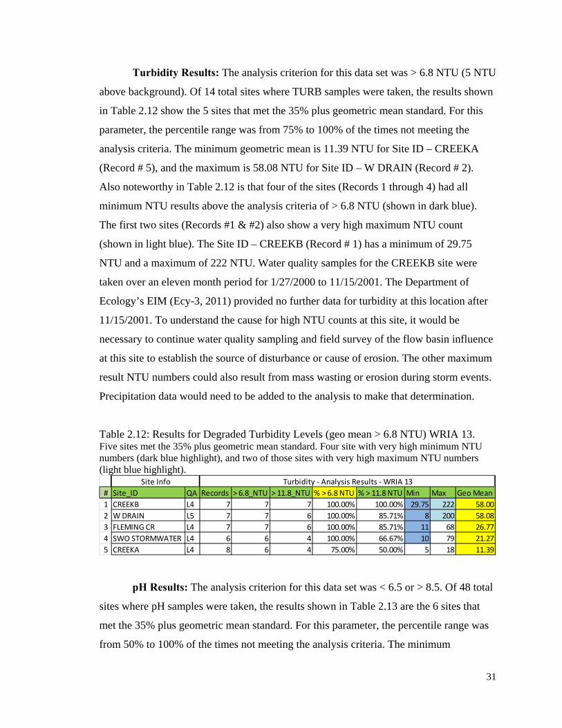
31

Turbidity Results: The analysis criterion for this data set was > 6.8 NTU (5 NTU

above background). Of 14 total sites where TURB samples were taken, the results shown

in Table 2.12 show the 5 sites that met the 35% plus geometric mean standard. For this

parameter, the percentile range was from 75% to 100% of the times not meeting the

analysis criteria. The minimum geometric mean is 11.39 NTU for Site ID – CREEKA

(Record # 5), and the maximum is 58.08 NTU for Site ID – W DRAIN (Record # 2).

Also noteworthy in Table 2.12 is that four of the sites (Records 1 through 4) had all

minimum NTU results above the analysis criteria of > 6.8 NTU (shown in dark blue).

The first two sites (Records #1 & #2) also show a very high maximum NTU count

(shown in light blue). The Site ID – CREEKB (Record # 1) has a minimum of 29.75

NTU and a maximum of 222 NTU. Water quality samples for the CREEKB site were

taken over an eleven month period for 1/27/2000 to 11/15/2001. The Department of

Ecology’s EIM (Ecy-3, 2011) provided no further data for turbidity at this location after

11/15/2001. To understand the cause for high NTU counts at this site, it would be

necessary to continue water quality sampling and field survey of the flow basin influence

at this site to establish the source of disturbance or cause of erosion. The other maximum

result NTU numbers could also result from mass wasting or erosion during storm events.

Precipitation data would need to be added to the analysis to make that determination.

Table 2.12: Results for Degraded Turbidity Levels (geo mean > 6.8 NTU) WRIA 13. Five sites met the 35% plus geometric mean standard. Four site with very high minimum NTU numbers (dark blue highlight), and two of those sites with very high maximum NTU numbers (light blue highlight).

# Site_ID QA Records > 6.8_NTU > 11.8_NTU % > 6.8 NTU % > 11.8 NTU Min Max Geo Mean1 CREEKB L4 7 7 7 100.00% 100.00% 29.75 222 58.002 W DRAIN L5 7 7 6 100.00% 85.71% 8 200 58.083 FLEMING CR L4 7 7 6 100.00% 85.71% 11 68 26.774 SWO STORMWATER L4 6 6 4 100.00% 66.67% 10 79 21.275 CREEKA L4 8 6 4 75.00% 50.00% 5 18 11.39

Site Info Turbidity - Analysis Results - WRIA 13

pH Results: The analysis criterion for this data set was < 6.5 or > 8.5. Of 48 total

sites where pH samples were taken, the results shown in Table 2.13 are the 6 sites that

met the 35% plus geometric mean standard. For this parameter, the percentile range was

from 50% to 100% of the times not meeting the analysis criteria. The minimum

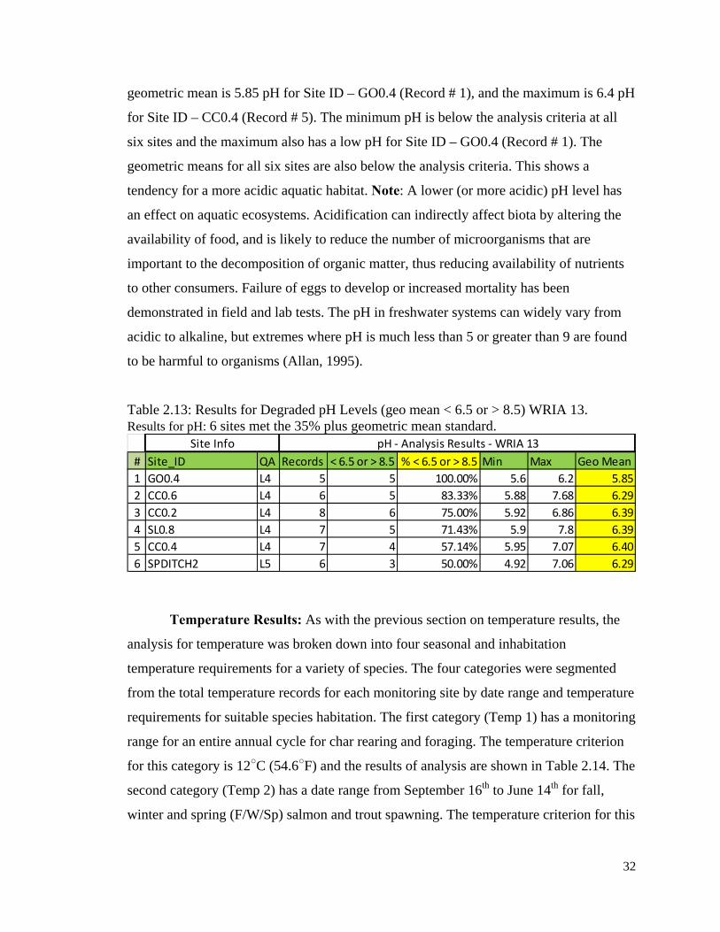
32

geometric mean is 5.85 pH for Site ID – GO0.4 (Record # 1), and the maximum is 6.4 pH

for Site ID – CC0.4 (Record # 5). The minimum pH is below the analysis criteria at all

six sites and the maximum also has a low pH for Site ID – GO0.4 (Record # 1). The

geometric means for all six sites are also below the analysis criteria. This shows a

tendency for a more acidic aquatic habitat. Note: A lower (or more acidic) pH level has

an effect on aquatic ecosystems. Acidification can indirectly affect biota by altering the

availability of food, and is likely to reduce the number of microorganisms that are

important to the decomposition of organic matter, thus reducing availability of nutrients

to other consumers. Failure of eggs to develop or increased mortality has been

demonstrated in field and lab tests. The pH in freshwater systems can widely vary from

acidic to alkaline, but extremes where pH is much less than 5 or greater than 9 are found

to be harmful to organisms (Allan, 1995).

Table 2.13: Results for Degraded pH Levels (geo mean < 6.5 or > 8.5) WRIA 13. Results for pH: 6 sites met the 35% plus geometric mean standard.

# Site_ID QA Records < 6.5 or > 8.5 % < 6.5 or > 8.5 Min Max Geo Mean1 GO0.4 L4 5 5 100.00% 5.6 6.2 5.852 CC0.6 L4 6 5 83.33% 5.88 7.68 6.293 CC0.2 L4 8 6 75.00% 5.92 6.86 6.394 SL0.8 L4 7 5 71.43% 5.9 7.8 6.395 CC0.4 L4 7 4 57.14% 5.95 7.07 6.406 SPDITCH2 L5 6 3 50.00% 4.92 7.06 6.29

Site Info pH - Analysis Results - WRIA 13

Temperature Results: As with the previous section on temperature results, the

analysis for temperature was broken down into four seasonal and inhabitation

temperature requirements for a variety of species. The four categories were segmented

from the total temperature records for each monitoring site by date range and temperature

requirements for suitable species habitation. The first category (Temp 1) has a monitoring

range for an entire annual cycle for char rearing and foraging. The temperature criterion

for this category is 12○C (54.6○F) and the results of analysis are shown in Table 2.14. The

second category (Temp 2) has a date range from September 16th to June 14th for fall,

winter and spring (F/W/Sp) salmon and trout spawning. The temperature criterion for this

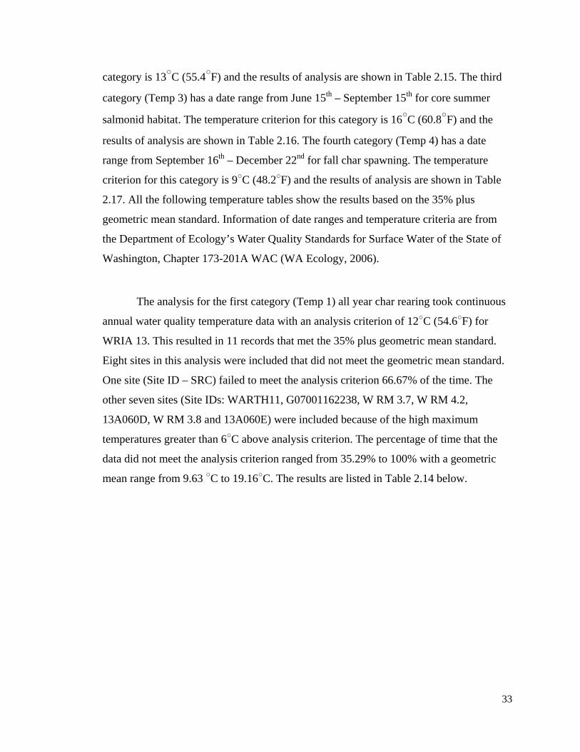
33

category is 13○C (55.4○F) and the results of analysis are shown in Table 2.15. The third

category (Temp 3) has a date range from June 15th – September 15th for core summer

salmonid habitat. The temperature criterion for this category is 16○C (60.8○F) and the

results of analysis are shown in Table 2.16. The fourth category (Temp 4) has a date

range from September 16th – December 22nd for fall char spawning. The temperature

criterion for this category is 9○C (48.2○F) and the results of analysis are shown in Table

2.17. All the following temperature tables show the results based on the 35% plus

geometric mean standard. Information of date ranges and temperature criteria are from

the Department of Ecology’s Water Quality Standards for Surface Water of the State of

Washington, Chapter 173-201A WAC (WA Ecology, 2006).

The analysis for the first category (Temp 1) all year char rearing took continuous

annual water quality temperature data with an analysis criterion of 12○C (54.6○F) for

WRIA 13. This resulted in 11 records that met the 35% plus geometric mean standard.

Eight sites in this analysis were included that did not meet the geometric mean standard.

One site (Site ID – SRC) failed to meet the analysis criterion 66.67% of the time. The

other seven sites (Site IDs: WARTH11, G07001162238, W RM 3.7, W RM 4.2,

13A060D, W RM 3.8 and 13A060E) were included because of the high maximum

temperatures greater than 6○C above analysis criterion. The percentage of time that the

data did not meet the analysis criterion ranged from 35.29% to 100% with a geometric

mean range from 9.63 ○C to 19.16○C. The results are listed in Table 2.14 below.

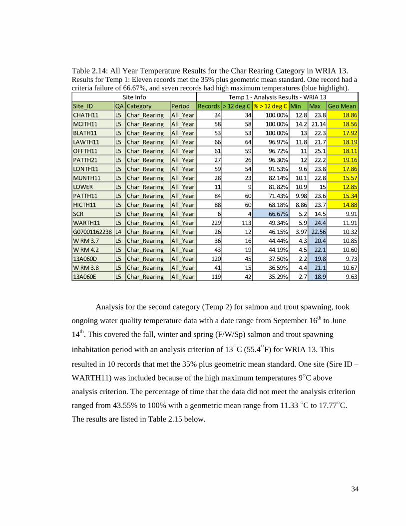
34

Table 2.14: All Year Temperature Results for the Char Rearing Category in WRIA 13. Results for Temp 1: Eleven records met the 35% plus geometric mean standard. One record had a criteria failure of 66.67%, and seven records had high maximum temperatures (blue highlight).

Site_ID QA Category Period Records > 12 deg C % > 12 deg C Min Max Geo MeanCHATH11 L5 Char_Rearing All_Year 34 34 100.00% 12.8 23.8 18.86MCITH11 L5 Char_Rearing All_Year 58 58 100.00% 14.2 21.14 18.56BLATH11 L5 Char_Rearing All_Year 53 53 100.00% 13 22.3 17.92LAWTH11 L5 Char_Rearing All_Year 66 64 96.97% 11.8 21.7 18.19OFFTH11 L5 Char_Rearing All_Year 61 59 96.72% 11 25.1 18.11PATTH21 L5 Char_Rearing All_Year 27 26 96.30% 12 22.2 19.16LONTH11 L5 Char_Rearing All_Year 59 54 91.53% 9.6 23.8 17.86MUNTH11 L5 Char_Rearing All_Year 28 23 82.14% 10.1 22.8 15.57LOWER L5 Char_Rearing All_Year 11 9 81.82% 10.9 15 12.85PATTH11 L5 Char_Rearing All_Year 84 60 71.43% 9.98 23.6 15.34HICTH11 L5 Char_Rearing All_Year 88 60 68.18% 8.86 23.7 14.88SCR L5 Char_Rearing All_Year 6 4 66.67% 5.2 14.5 9.91WARTH11 L5 Char_Rearing All_Year 229 113 49.34% 5.9 24.4 11.91G07001162238 L4 Char_Rearing All_Year 26 12 46.15% 3.97 22.56 10.32W RM 3.7 L5 Char_Rearing All_Year 36 16 44.44% 4.3 20.4 10.85W RM 4.2 L5 Char_Rearing All_Year 43 19 44.19% 4.5 22.1 10.6013A060D L5 Char_Rearing All_Year 120 45 37.50% 2.2 19.8 9.73W RM 3.8 L5 Char_Rearing All_Year 41 15 36.59% 4.4 21.1 10.6713A060E L5 Char_Rearing All_Year 119 42 35.29% 2.7 18.9 9.63


Analysis for the second category (Temp 2) for salmon and trout spawning, took

ongoing water quality temperature data with a date range from September 16th to June

14th. This covered the fall, winter and spring (F/W/Sp) salmon and trout spawning

inhabitation period with an analysis criterion of 13○C (55.4○F) for WRIA 13. This

resulted in 10 records that met the 35% plus geometric mean standard. One site (Sire ID –

WARTH11) was included because of the high maximum temperatures 9○C above

analysis criterion. The percentage of time that the data did not meet the analysis criterion

ranged from 43.55% to 100% with a geometric mean range from 11.33 ○C to 17.77○C.

The results are listed in Table 2.15 below.

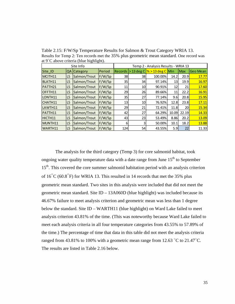
35

Table 2.15: F/W/Sp Temperature Results for Salmon & Trout Category WRIA 13. Results for Temp 2: Ten records met the 35% plus geometric mean standard. One record was at 9○C above criteria (blue highlight).

Site_ID QA Category Period Records > 13 deg C % > 13 deg C Min Max Geo MeanMCITH11 L5 Salmon/Trout F/W/Sp 38 38 100.00% 14.2 20.9 17.77BLATH11 L5 Salmon/Trout F/W/Sp 35 34 97.14% 13 19.9 16.97PATTH21 L5 Salmon/Trout F/W/Sp 11 10 90.91% 12 21 17.60OFFTH11 L5 Salmon/Trout F/W/Sp 29 26 89.66% 11 22.2 16.91LONTH11 L5 Salmon/Trout F/W/Sp 35 27 77.14% 9.6 20.8 15.95CHATH11 L5 Salmon/Trout F/W/Sp 13 10 76.92% 12.8 23.8 17.11LAWTH11 L5 Salmon/Trout F/W/Sp 29 21 72.41% 11.8 20 15.34PATTH11 L5 Salmon/Trout F/W/Sp 42 27 64.29% 10.09 22.19 14.33HICTH11 L5 Salmon/Trout F/W/Sp 43 23 53.49% 8.86 20.2 13.09MUNTH11 L5 Salmon/Trout F/W/Sp 6 3 50.00% 10.1 18.2 13.88WARTH11 L5 Salmon/Trout F/W/Sp 124 54 43.55% 5.9 22 11.33


The analysis for the third category (Temp 3) for core salmonid habitat, took

ongoing water quality temperature data with a date range from June 15th to September

15th. This covered the core summer salmonid habitation period with an analysis criterion

of 16○C (60.8○F) for WRIA 13. This resulted in 14 records that met the 35% plus

geometric mean standard. Two sites in this analysis were included that did not meet the

geometric mean standard. Site ID – 13A060D (blue highlight) was included because its

46.67% failure to meet analysis criterion and geometric mean was less than 1 degree

below the standard. Site ID – WARTH11 (blue highlight) on Ward Lake failed to meet

analysis criterion 43.81% of the time. (This was noteworthy because Ward Lake failed to

meet each analysis criteria in all four temperature categories from 43.55% to 57.89% of

the time.) The percentage of time that data in this table did not meet the analysis criteria

ranged from 43.81% to 100% with a geometric mean range from 12.63 ○C to 21.47○C.

The results are listed in Table 2.16 below.

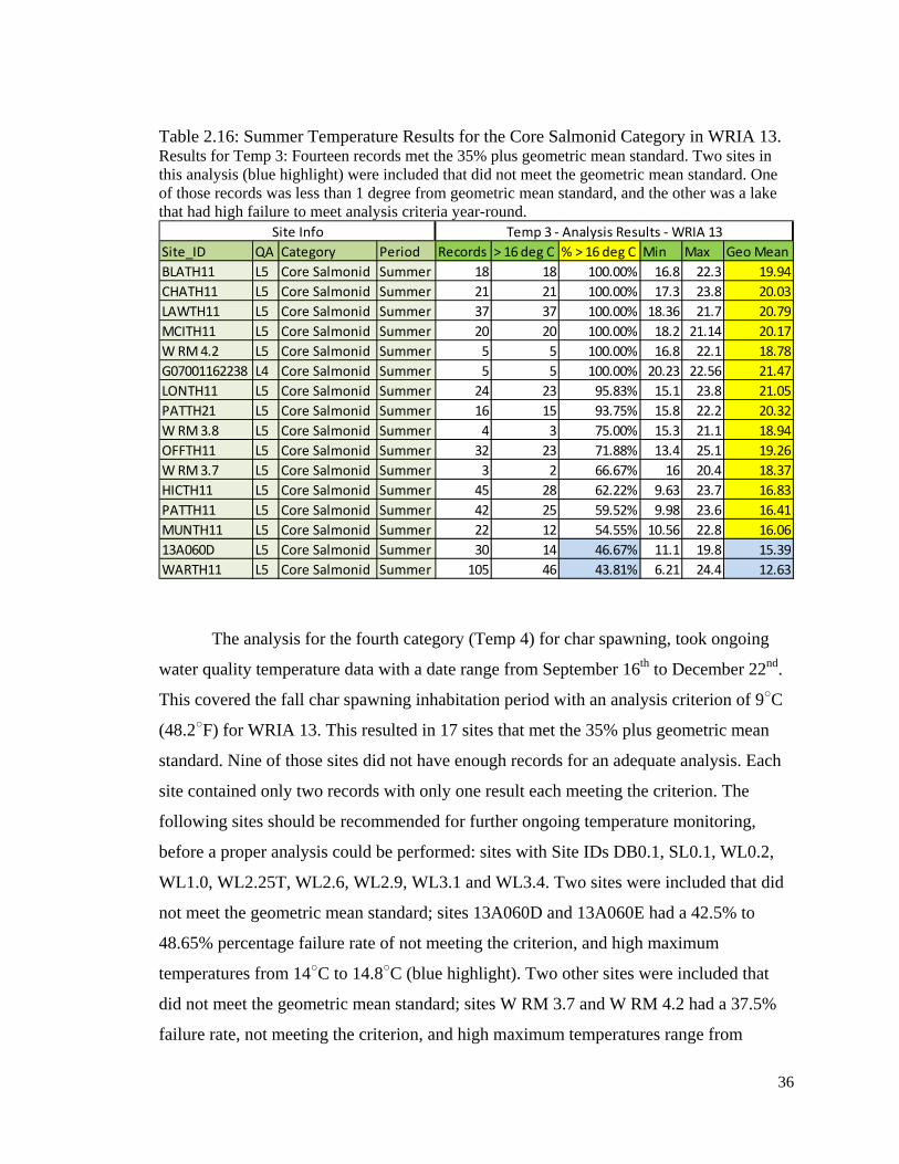
36

Table 2.16: Summer Temperature Results for the Core Salmonid Category in WRIA 13. Results for Temp 3: Fourteen records met the 35% plus geometric mean standard. Two sites in this analysis (blue highlight) were included that did not meet the geometric mean standard. One of those records was less than 1 degree from geometric mean standard, and the other was a lake that had high failure to meet analysis criteria year-round.

Site_ID QA Category Period Records > 16 deg C % > 16 deg C Min Max Geo MeanBLATH11 L5 Core Salmonid Summer 18 18 100.00% 16.8 22.3 19.94CHATH11 L5 Core Salmonid Summer 21 21 100.00% 17.3 23.8 20.03LAWTH11 L5 Core Salmonid Summer 37 37 100.00% 18.36 21.7 20.79MCITH11 L5 Core Salmonid Summer 20 20 100.00% 18.2 21.14 20.17W RM 4.2 L5 Core Salmonid Summer 5 5 100.00% 16.8 22.1 18.78G07001162238 L4 Core Salmonid Summer 5 5 100.00% 20.23 22.56 21.47LONTH11 L5 Core Salmonid Summer 24 23 95.83% 15.1 23.8 21.05PATTH21 L5 Core Salmonid Summer 16 15 93.75% 15.8 22.2 20.32W RM 3.8 L5 Core Salmonid Summer 4 3 75.00% 15.3 21.1 18.94OFFTH11 L5 Core Salmonid Summer 32 23 71.88% 13.4 25.1 19.26W RM 3.7 L5 Core Salmonid Summer 3 2 66.67% 16 20.4 18.37HICTH11 L5 Core Salmonid Summer 45 28 62.22% 9.63 23.7 16.83PATTH11 L5 Core Salmonid Summer 42 25 59.52% 9.98 23.6 16.41MUNTH11 L5 Core Salmonid Summer 22 12 54.55% 10.56 22.8 16.0613A060D L5 Core Salmonid Summer 30 14 46.67% 11.1 19.8 15.39WARTH11 L5 Core Salmonid Summer 105 46 43.81% 6.21 24.4 12.63


The analysis for the fourth category (Temp 4) for char spawning, took ongoing

water quality temperature data with a date range from September 16th to December 22nd.

This covered the fall char spawning inhabitation period with an analysis criterion of 9○C

(48.2○F) for WRIA 13. This resulted in 17 sites that met the 35% plus geometric mean

standard. Nine of those sites did not have enough records for an adequate analysis. Each

site contained only two records with only one result each meeting the criterion. The

following sites should be recommended for further ongoing temperature monitoring,

before a proper analysis could be performed: sites with Site IDs DB0.1, SL0.1, WL0.2,

WL1.0, WL2.25T, WL2.6, WL2.9, WL3.1 and WL3.4. Two sites were included that did

not meet the geometric mean standard; sites 13A060D and 13A060E had a 42.5% to

48.65% percentage failure rate of not meeting the criterion, and high maximum

temperatures from 14○C to 14.8○C (blue highlight). Two other sites were included that

did not meet the geometric mean standard; sites W RM 3.7 and W RM 4.2 had a 37.5%

failure rate, not meeting the criterion, and high maximum temperatures range from

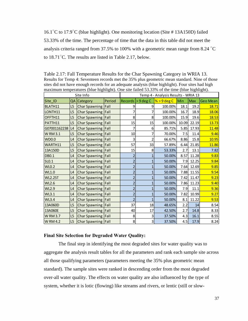
37

16.1○C to 17.9○C (blue highlight). One monitoring location (Site # 13A150D) failed

53.33% of the time. The percentage of time that the data in this table did not meet the

analysis criteria ranged from 37.5% to 100% with a geometric mean range from 8.24 ○C

to 18.71○C. The results are listed in Table 2.17, below.

Table 2.17: Fall Temperature Results for the Char Spawning Category in WRIA 13. Results for Temp 4: Seventeen records met the 35% plus geometric mean standard. Nine of those sites did not have enough records for an adequate analysis (blue highlight). Four sites had high maximum temperatures (blue highlight). One site failed 53.33% of the time (blue highlight).

Site_ID QA Category Period Records > 9 deg C % > 9 deg C Min Max Geo MeanBLATH11 L5 Char Spawning Fall 9 9 100.00% 18.1 19.2 18.71LONTH11 L5 Char Spawning Fall 7 7 100.00% 16.7 18.9 18.06OFFTH11 L5 Char Spawning Fall 8 8 100.00% 15.9 19.6 18.53PATTH11 L5 Char Spawning Fall 15 15 100.00% 10.09 22.19 13.73G07001162238 L4 Char Spawning Fall 7 6 85.71% 5.85 17.93 11.48W RM 3.1 L5 Char Spawning Fall 10 7 70.00% 7.5 11.4 9.46WD0.0 L4 Char Spawning Fall 3 2 66.67% 8.86 15.8 10.95WARTH11 L5 Char Spawning Fall 57 33 57.89% 6.44 21.85 11.8613A150D L5 Char Spawning Fall 15 8 53.33% 2.7 13.1 7.82DB0.1 L4 Char Spawning Fall 2 1 50.00% 8.57 11.28 9.83SL0.1 L4 Char Spawning Fall 2 1 50.00% 7.9 12.25 9.84WL0.2 L4 Char Spawning Fall 2 1 50.00% 7.64 12.69 9.85WL1.0 L4 Char Spawning Fall 2 1 50.00% 7.88 11.55 9.54WL2.25T L4 Char Spawning Fall 2 1 50.00% 7.42 11.47 9.23WL2.6 L4 Char Spawning Fall 2 1 50.00% 7.86 11.23 9.40WL2.9 L4 Char Spawning Fall 2 1 50.00% 7.9 11.1 9.36WL3.1 L4 Char Spawning Fall 2 1 50.00% 7.82 10.99 9.27WL3.4 L4 Char Spawning Fall 2 1 50.00% 8.1 11.22 9.5313A060D L5 Char Spawning Fall 37 18 48.65% 2.2 14 8.5413A060E L5 Char Spawning Fall 40 17 42.50% 2.7 14.8 8.33W RM 3.7 L5 Char Spawning Fall 8 3 37.50% 4.3 16.1 8.55W RM 4.2 L5 Char Spawning Fall 8 3 37.50% 4.5 17.9 8.24


Final Site Selection for Degraded Water Quality:

The final step in identifying the most degraded sites for water quality was to

aggregate the analysis result tables for all the parameters and rank each sample site across

all those qualifying parameters (parameters meeting the 35% plus geometric mean

standard). The sample sites were ranked in descending order from the most degraded

over-all water quality. The effects on water quality are also influenced by the type of

system, whether it is lotic (flowing) like streams and rivers, or lentic (still or slow-

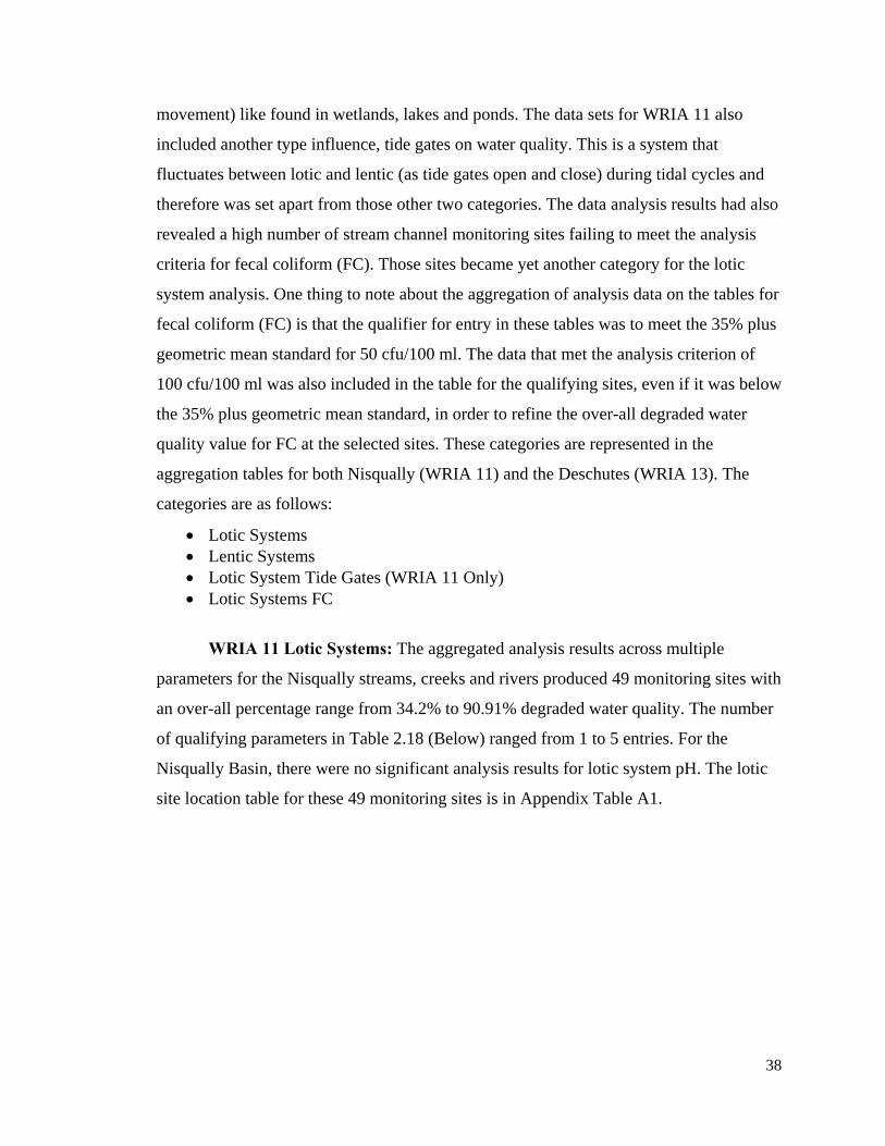
38

movement) like found in wetlands, lakes and ponds. The data sets for WRIA 11 also

included another type influence, tide gates on water quality. This is a system that

fluctuates between lotic and lentic (as tide gates open and close) during tidal cycles and

therefore was set apart from those other two categories. The data analysis results had also

revealed a high number of stream channel monitoring sites failing to meet the analysis

criteria for fecal coliform (FC). Those sites became yet another category for the lotic

system analysis. One thing to note about the aggregation of analysis data on the tables for

fecal coliform (FC) is that the qualifier for entry in these tables was to meet the 35% plus

geometric mean standard for 50 cfu/100 ml. The data that met the analysis criterion of

100 cfu/100 ml was also included in the table for the qualifying sites, even if it was below

the 35% plus geometric mean standard, in order to refine the over-all degraded water

quality value for FC at the selected sites. These categories are represented in the

aggregation tables for both Nisqually (WRIA 11) and the Deschutes (WRIA 13). The

categories are as follows:

Lotic Systems Lentic Systems Lotic System Tide Gates (WRIA 11 Only) Lotic Systems FC

WRIA 11 Lotic Systems: The aggregated analysis results across multiple

parameters for the Nisqually streams, creeks and rivers produced 49 monitoring sites with

an over-all percentage range from 34.2% to 90.91% degraded water quality. The number

of qualifying parameters in Table 2.18 (Below) ranged from 1 to 5 entries. For the

Nisqually Basin, there were no significant analysis results for lotic system pH. The lotic

site location table for these 49 monitoring sites is in Appendix Table A1.

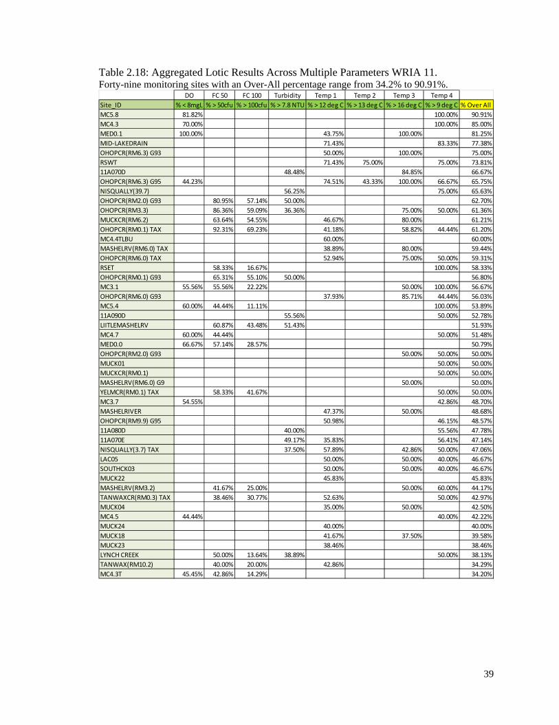
39

Table 2.18: Aggregated Lotic Results Across Multiple Parameters WRIA 11. Forty-nine monitoring sites with an Over-All percentage range from 34.2% to 90.91%.

DO FC 50 FC 100 Turbidity Temp 1 Temp 2 Temp 3 Temp 4Site_ID % < 8mgL % > 50cfu % > 100cfu % > 7.8 NTU % > 12 deg C % > 13 deg C % > 16 deg C % > 9 deg C % Over AllMC5.8 81.82% 100.00% 90.91%MC4.3 70.00% 100.00% 85.00%MED0.1 100.00% 43.75% 100.00% 81.25%MID-LAKEDRAIN 71.43% 83.33% 77.38%OHOPCR(RM6.3) G93 50.00% 100.00% 75.00%RSWT 71.43% 75.00% 75.00% 73.81%11A070D 48.48% 84.85% 66.67%OHOPCR(RM6.3) G95 44.23% 74.51% 43.33% 100.00% 66.67% 65.75%NISQUALLY(39.7) 56.25% 75.00% 65.63%OHOPCR(RM2.0) G93 80.95% 57.14% 50.00% 62.70%OHOPCR(RM3.3) 86.36% 59.09% 36.36% 75.00% 50.00% 61.36%MUCKCR(RM6.2) 63.64% 54.55% 46.67% 80.00% 61.21%OHOPCR(RM0.1) TAX 92.31% 69.23% 41.18% 58.82% 44.44% 61.20%MC4.4TLBU 60.00% 60.00%MASHELRV(RM6.0) TAX 38.89% 80.00% 59.44%OHOPCR(RM6.0) TAX 52.94% 75.00% 50.00% 59.31%RSET 58.33% 16.67% 100.00% 58.33%OHOPCR(RM0.1) G93 65.31% 55.10% 50.00% 56.80%MC3.1 55.56% 55.56% 22.22% 50.00% 100.00% 56.67%OHOPCR(RM6.0) G93 37.93% 85.71% 44.44% 56.03%MC5.4 60.00% 44.44% 11.11% 100.00% 53.89%11A090D 55.56% 50.00% 52.78%LIITLEMASHELRV 60.87% 43.48% 51.43% 51.93%MC4.7 60.00% 44.44% 50.00% 51.48%MED0.0 66.67% 57.14% 28.57% 50.79%OHOPCR(RM2.0) G93 50.00% 50.00% 50.00%MUCK01 50.00% 50.00%MUCKCR(RM0.1) 50.00% 50.00%MASHELRV(RM6.0) G9 50.00% 50.00%YELMCR(RM0.1) TAX 58.33% 41.67% 50.00% 50.00%MC3.7 54.55% 42.86% 48.70%MASHELRIVER 47.37% 50.00% 48.68%OHOPCR(RM9.9) G95 50.98% 46.15% 48.57%11A080D 40.00% 55.56% 47.78%11A070E 49.17% 35.83% 56.41% 47.14%NISQUALLY(3.7) TAX 37.50% 57.89% 42.86% 50.00% 47.06%LAC05 50.00% 50.00% 40.00% 46.67%SOUTHCK03 50.00% 50.00% 40.00% 46.67%MUCK22 45.83% 45.83%MASHELRV(RM3.2) 41.67% 25.00% 50.00% 60.00% 44.17%TANWAXCR(RM0.3) TAX 38.46% 30.77% 52.63% 50.00% 42.97%MUCK04 35.00% 50.00% 42.50%MC4.5 44.44% 40.00% 42.22%MUCK24 40.00% 40.00%MUCK18 41.67% 37.50% 39.58%MUCK23 38.46% 38.46%LYNCH CREEK 50.00% 13.64% 38.89% 50.00% 38.13%TANWAX(RM10.2) 40.00% 20.00% 42.86% 34.29%MC4.3T 45.45% 42.86% 14.29% 34.20%

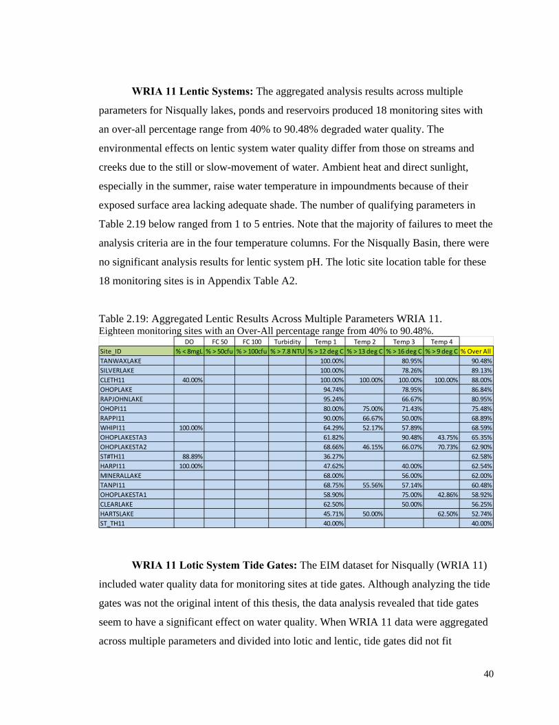
40

WRIA 11 Lentic Systems: The aggregated analysis results across multiple

parameters for Nisqually lakes, ponds and reservoirs produced 18 monitoring sites with

an over-all percentage range from 40% to 90.48% degraded water quality. The

environmental effects on lentic system water quality differ from those on streams and

creeks due to the still or slow-movement of water. Ambient heat and direct sunlight,

especially in the summer, raise water temperature in impoundments because of their

exposed surface area lacking adequate shade. The number of qualifying parameters in

Table 2.19 below ranged from 1 to 5 entries. Note that the majority of failures to meet the

analysis criteria are in the four temperature columns. For the Nisqually Basin, there were

no significant analysis results for lentic system pH. The lotic site location table for these

18 monitoring sites is in Appendix Table A2.

Table 2.19: Aggregated Lentic Results Across Multiple Parameters WRIA 11. Eighteen monitoring sites with an Over-All percentage range from 40% to 90.48%.

DO FC 50 FC 100 Turbidity Temp 1 Temp 2 Temp 3 Temp 4Site_ID % < 8mgL % > 50cfu % > 100cfu % > 7.8 NTU % > 12 deg C % > 13 deg C % > 16 deg C % > 9 deg C % Over AllTANWAXLAKE 100.00% 80.95% 90.48%SILVERLAKE 100.00% 78.26% 89.13%CLETH11 40.00% 100.00% 100.00% 100.00% 100.00% 88.00%OHOPLAKE 94.74% 78.95% 86.84%RAPJOHNLAKE 95.24% 66.67% 80.95%OHOPI11 80.00% 75.00% 71.43% 75.48%RAPPI11 90.00% 66.67% 50.00% 68.89%WHIPI11 100.00% 64.29% 52.17% 57.89% 68.59%OHOPLAKESTA3 61.82% 90.48% 43.75% 65.35%OHOPLAKESTA2 68.66% 46.15% 66.07% 70.73% 62.90%ST#TH11 88.89% 36.27% 62.58%HARPI11 100.00% 47.62% 40.00% 62.54%MINERALLAKE 68.00% 56.00% 62.00%TANPI11 68.75% 55.56% 57.14% 60.48%OHOPLAKESTA1 58.90% 75.00% 42.86% 58.92%CLEARLAKE 62.50% 50.00% 56.25%HARTSLAKE 45.71% 50.00% 62.50% 52.74%ST_TH11 40.00% 40.00%

WRIA 11 Lotic System Tide Gates: The EIM dataset for Nisqually (WRIA 11)

included water quality data for monitoring sites at tide gates. Although analyzing the tide

gates was not the original intent of this thesis, the data analysis revealed that tide gates

seem to have a significant effect on water quality. When WRIA 11 data were aggregated

across multiple parameters and divided into lotic and lentic, tide gates did not fit

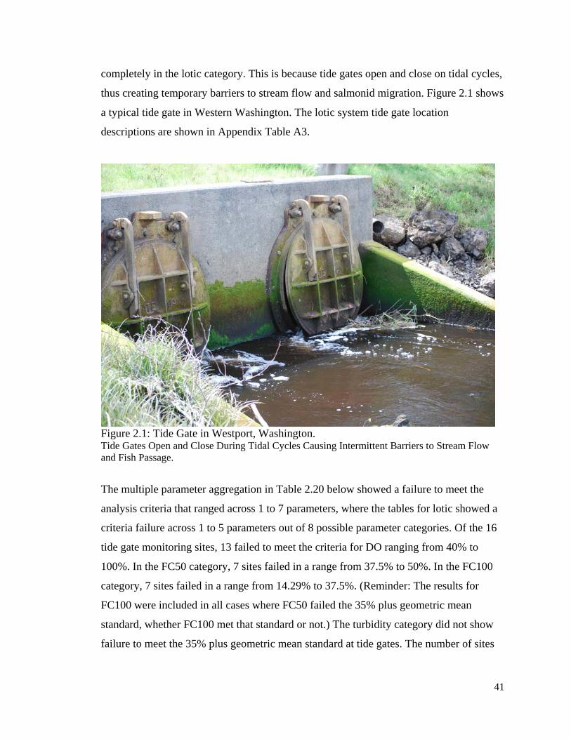
41

completely in the lotic category. This is because tide gates open and close on tidal cycles,

thus creating temporary barriers to stream flow and salmonid migration. Figure 2.1 shows

a typical tide gate in Western Washington. The lotic system tide gate location

descriptions are shown in Appendix Table A3.

Figure 2.1: Tide Gate in Westport, Washington. Tide Gates Open and Close During Tidal Cycles Causing Intermittent Barriers to Stream Flow and Fish Passage.

The multiple parameter aggregation in Table 2.20 below showed a failure to meet the

analysis criteria that ranged across 1 to 7 parameters, where the tables for lotic showed a

criteria failure across 1 to 5 parameters out of 8 possible parameter categories. Of the 16

tide gate monitoring sites, 13 failed to meet the criteria for DO ranging from 40% to

100%. In the FC50 category, 7 sites failed in a range from 37.5% to 50%. In the FC100

category, 7 sites failed in a range from 14.29% to 37.5%. (Reminder: The results for

FC100 were included in all cases where FC50 failed the 35% plus geometric mean

standard, whether FC100 met that standard or not.) The turbidity category did not show

failure to meet the 35% plus geometric mean standard at tide gates. The number of sites

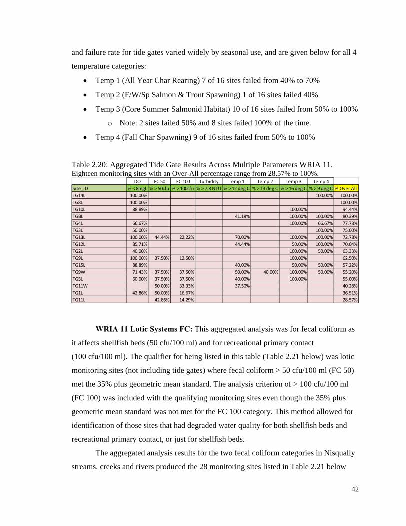
42

and failure rate for tide gates varied widely by seasonal use, and are given below for all 4

temperature categories:

Temp 1 (All Year Char Rearing) 7 of 16 sites failed from 40% to 70%

Temp 2 (F/W/Sp Salmon & Trout Spawning) 1 of 16 sites failed 40%

Temp 3 (Core Summer Salmonid Habitat) 10 of 16 sites failed from 50% to 100%

o Note: 2 sites failed 50% and 8 sites failed 100% of the time.

Temp 4 (Fall Char Spawning) 9 of 16 sites failed from 50% to 100%

Table 2.20: Aggregated Tide Gate Results Across Multiple Parameters WRIA 11. Eighteen monitoring sites with an Over-All percentage range from 28.57% to 100%.

DO FC 50 FC 100 Turbidity Temp 1 Temp 2 Temp 3 Temp 4Site_ID % < 8mgL % > 50cfu % > 100cfu % > 7.8 NTU % > 12 deg C % > 13 deg C % > 16 deg C % > 9 deg C % Over AllTG14L 100.00% 100.00% 100.00%TG8L 100.00% 100.00%TG10L 88.89% 100.00% 94.44%TGBL 41.18% 100.00% 100.00% 80.39%TG4L 66.67% 100.00% 66.67% 77.78%TG3L 50.00% 100.00% 75.00%TG13L 100.00% 44.44% 22.22% 70.00% 100.00% 100.00% 72.78%TG12L 85.71% 44.44% 50.00% 100.00% 70.04%TG2L 40.00% 100.00% 50.00% 63.33%TG9L 100.00% 37.50% 12.50% 100.00% 62.50%TG15L 88.89% 40.00% 50.00% 50.00% 57.22%TG9W 71.43% 37.50% 37.50% 50.00% 40.00% 100.00% 50.00% 55.20%TG5L 60.00% 37.50% 37.50% 40.00% 100.00% 55.00%TG11W 50.00% 33.33% 37.50% 40.28%TG1L 42.86% 50.00% 16.67% 36.51%TG11L 42.86% 14.29% 28.57%

WRIA 11 Lotic Systems FC: This aggregated analysis was for fecal coliform as

it affects shellfish beds (50 cfu/100 ml) and for recreational primary contact

(100 cfu/100 ml). The qualifier for being listed in this table (Table 2.21 below) was lotic

monitoring sites (not including tide gates) where fecal coliform > 50 cfu/100 ml (FC 50)

met the 35% plus geometric mean standard. The analysis criterion of > 100 cfu/100 ml

(FC 100) was included with the qualifying monitoring sites even though the 35% plus

geometric mean standard was not met for the FC 100 category. This method allowed for

identification of those sites that had degraded water quality for both shellfish beds and

recreational primary contact, or just for shellfish beds.

The aggregated analysis results for the two fecal coliform categories in Nisqually

streams, creeks and rivers produced the 28 monitoring sites listed in Table 2.21 below

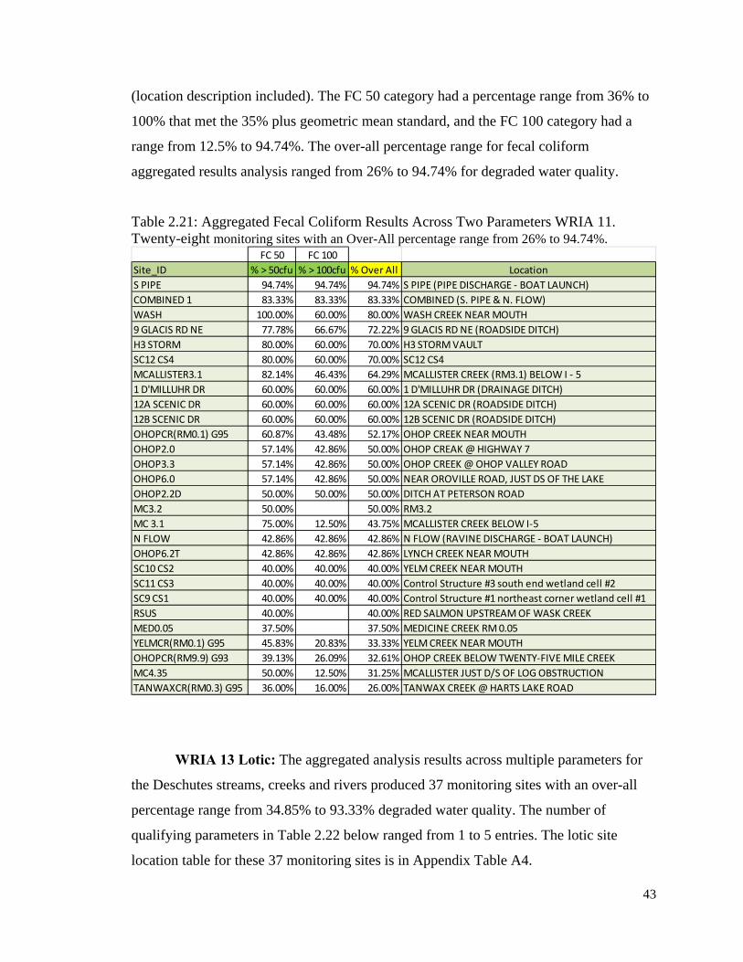
43

(location description included). The FC 50 category had a percentage range from 36% to

100% that met the 35% plus geometric mean standard, and the FC 100 category had a

range from 12.5% to 94.74%. The over-all percentage range for fecal coliform

aggregated results analysis ranged from 26% to 94.74% for degraded water quality.

Table 2.21: Aggregated Fecal Coliform Results Across Two Parameters WRIA 11. Twenty-eight monitoring sites with an Over-All percentage range from 26% to 94.74%.

FC 50 FC 100Site_ID % > 50cfu % > 100cfu % Over All LocationS PIPE 94.74% 94.74% 94.74% S PIPE (PIPE DISCHARGE - BOAT LAUNCH)COMBINED 1 83.33% 83.33% 83.33% COMBINED (S. PIPE & N. FLOW)WASH 100.00% 60.00% 80.00% WASH CREEK NEAR MOUTH9 GLACIS RD NE 77.78% 66.67% 72.22% 9 GLACIS RD NE (ROADSIDE DITCH)H3 STORM 80.00% 60.00% 70.00% H3 STORM VAULTSC12 CS4 80.00% 60.00% 70.00% SC12 CS4MCALLISTER3.1 82.14% 46.43% 64.29% MCALLISTER CREEK (RM3.1) BELOW I - 51 D'MILLUHR DR 60.00% 60.00% 60.00% 1 D'MILLUHR DR (DRAINAGE DITCH)12A SCENIC DR 60.00% 60.00% 60.00% 12A SCENIC DR (ROADSIDE DITCH)12B SCENIC DR 60.00% 60.00% 60.00% 12B SCENIC DR (ROADSIDE DITCH)OHOPCR(RM0.1) G95 60.87% 43.48% 52.17% OHOP CREEK NEAR MOUTHOHOP2.0 57.14% 42.86% 50.00% OHOP CREAK @ HIGHWAY 7OHOP3.3 57.14% 42.86% 50.00% OHOP CREEK @ OHOP VALLEY ROADOHOP6.0 57.14% 42.86% 50.00% NEAR OROVILLE ROAD, JUST DS OF THE LAKEOHOP2.2D 50.00% 50.00% 50.00% DITCH AT PETERSON ROADMC3.2 50.00% 50.00% RM3.2MC 3.1 75.00% 12.50% 43.75% MCALLISTER CREEK BELOW I-5N FLOW 42.86% 42.86% 42.86% N FLOW (RAVINE DISCHARGE - BOAT LAUNCH)OHOP6.2T 42.86% 42.86% 42.86% LYNCH CREEK NEAR MOUTHSC10 CS2 40.00% 40.00% 40.00% YELM CREEK NEAR MOUTHSC11 CS3 40.00% 40.00% 40.00% Control Structure #3 south end wetland cell #2SC9 CS1 40.00% 40.00% 40.00% Control Structure #1 northeast corner wetland cell #1RSUS 40.00% 40.00% RED SALMON UPSTREAM OF WASK CREEKMED0.05 37.50% 37.50% MEDICINE CREEK RM 0.05YELMCR(RM0.1) G95 45.83% 20.83% 33.33% YELM CREEK NEAR MOUTHOHOPCR(RM9.9) G93 39.13% 26.09% 32.61% OHOP CREEK BELOW TWENTY-FIVE MILE CREEKMC4.35 50.00% 12.50% 31.25% MCALLISTER JUST D/S OF LOG OBSTRUCTIONTANWAXCR(RM0.3) G95 36.00% 16.00% 26.00% TANWAX CREEK @ HARTS LAKE ROAD

WRIA 13 Lotic: The aggregated analysis results across multiple parameters for

the Deschutes streams, creeks and rivers produced 37 monitoring sites with an over-all

percentage range from 34.85% to 93.33% degraded water quality. The number of

qualifying parameters in Table 2.22 below ranged from 1 to 5 entries. The lotic site

location table for these 37 monitoring sites is in Appendix Table A4.

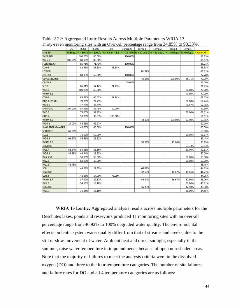
44

Table 2.22: Aggregated Lotic Results Across Multiple Parameters WRIA 13. Thirty-seven monitoring sites with an Over-All percentage range from 34.85% to 93.33%.

DO FC 50 FC 100 pH Turbidity Temp 1 Temp 2 Temp 3 Temp 4Site_ID % 8mgL % > 50cfu % > 100cfu % < 6.5 or > 8.5 % > 7.8 NTU % > 12 deg C % > 13 deg C % > 16 deg C % > 9 deg C % Over AllW DRAIN 100.00% 80.00% 100.00% 93.33%WD6.8 100.00% 80.00% 80.00% 86.67%FLEMING CR 85.71% 71.43% 100.00% 85.71%CC0.6 83.33% 83.33% 83.33% 83.33%LOWER 81.82% 81.82%CREEKB 83.33% 50.00% 100.00% 77.78%G07001162238 46.15% 100.00% 85.71% 77.29%CREEKA 75.00% 75.00%SL0.8 85.71% 57.14% 71.43% 71.43%WL1.0 100.00% 60.00% 50.00% 70.00%W RM 3.1 70.00% 70.00%CC0.4 83.33% 66.67% 57.14% 69.05%DB0.1 (DSAR) 70.00% 72.73% 50.00% 64.24%WD0.0 77.78% 44.44% 66.67% 62.96%SPDITCH2 100.00% 54.55% 45.45% 50.00% 62.50%WL0.2 75.00% 58.33% 50.00% 61.11%GO0.4 50.00% 33.33% 100.00% 61.11%W RM 4.2 44.19% 100.00% 37.50% 60.56%WD5.1 25.00% 88.89% 66.67% 60.19%SWO STORMWATER 40.00% 40.00% 100.00% 60.00%SPDITCH1 60.00% 60.00%SL0.1 70.00% 50.00% 50.00% 56.67%WD6.9 91.67% 55.56% 22.22% 56.48%W RM 3.8 36.59% 75.00% 55.79%13A150D 53.33% 53.33%WL3.4 61.54% 54.55% 36.36% 50.00% 50.61%WD6.2 83.33% 44.44% 22.22% 50.00%WL2.25T 50.00% 50.00% 50.00% 50.00%WL2.6 60.00% 40.00% 50.00% 50.00%WL1.9T 45.45% 45.45%SCR 44.26% 22.95% 66.67% 44.63%13A060D 37.50% 46.67% 48.65% 44.27%CC0.2 42.86% 14.29% 75.00% 44.05%W RM 3.7 37.50% 29.17% 44.44% 66.67% 37.50% 43.06%WL2.9 54.55% 18.18% 50.00% 40.91%13A060E 35.29% 42.50% 38.90%WL3.1 36.36% 18.18% 50.00% 34.85%

WRIA 13 Lentic: Aggregated analysis results across multiple parameters for the

Deschutes lakes, ponds and reservoirs produced 11 monitoring sites with an over-all

percentage range from 46.92% to 100% degraded water quality. The environmental

effects on lentic system water quality differ from that of streams and creeks, due to the

still or slow-movement of water. Ambient heat and direct sunlight, especially in the

summer, raise water temperature in impoundments, because of open non-shaded areas.

Note that the majority of failures to meet the analysis criteria were in the dissolved

oxygen (DO) and three to the four temperature categories. The number of site failures

and failure rates for DO and all 4 temperature categories are as follows:

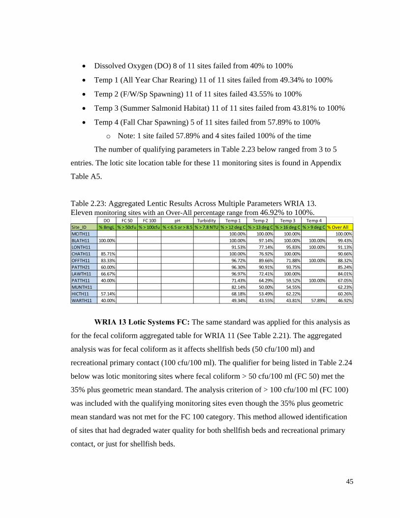
45

Dissolved Oxygen (DO) 8 of 11 sites failed from 40% to 100%

Temp 1 (All Year Char Rearing) 11 of 11 sites failed from 49.34% to 100%

Temp 2 (F/W/Sp Spawning) 11 of 11 sites failed 43.55% to 100%

Temp 3 (Summer Salmonid Habitat) 11 of 11 sites failed from 43.81% to 100%

Temp 4 (Fall Char Spawning) 5 of 11 sites failed from 57.89% to 100%

o Note: 1 site failed 57.89% and 4 sites failed 100% of the time

The number of qualifying parameters in Table 2.23 below ranged from 3 to 5

entries. The lotic site location table for these 11 monitoring sites is found in Appendix

Table A5.

Table 2.23: Aggregated Lentic Results Across Multiple Parameters WRIA 13. Eleven monitoring sites with an Over-All percentage range from 46.92% to 100%.

DO FC 50 FC 100 pH Turbidity Temp 1 Temp 2 Temp 3 Temp 4Site_ID % 8mgL % > 50cfu % > 100cfu % < 6.5 or > 8.5 % > 7.8 NTU % > 12 deg C % > 13 deg C % > 16 deg C % > 9 deg C % Over AllMCITH11 100.00% 100.00% 100.00% 100.00%BLATH11 100.00% 100.00% 97.14% 100.00% 100.00% 99.43%LONTH11 91.53% 77.14% 95.83% 100.00% 91.13%CHATH11 85.71% 100.00% 76.92% 100.00% 90.66%OFFTH11 83.33% 96.72% 89.66% 71.88% 100.00% 88.32%PATTH21 60.00% 96.30% 90.91% 93.75% 85.24%LAWTH11 66.67% 96.97% 72.41% 100.00% 84.01%PATTH11 40.00% 71.43% 64.29% 59.52% 100.00% 67.05%MUNTH11 82.14% 50.00% 54.55% 62.23%HICTH11 57.14% 68.18% 53.49% 62.22% 60.26%WARTH11 40.00% 49.34% 43.55% 43.81% 57.89% 46.92%

WRIA 13 Lotic Systems FC: The same standard was applied for this analysis as

for the fecal coliform aggregated table for WRIA 11 (See Table 2.21). The aggregated

analysis was for fecal coliform as it affects shellfish beds (50 cfu/100 ml) and

recreational primary contact (100 cfu/100 ml). The qualifier for being listed in Table 2.24

below was lotic monitoring sites where fecal coliform > 50 cfu/100 ml (FC 50) met the

35% plus geometric mean standard. The analysis criterion of > 100 cfu/100 ml (FC 100)

was included with the qualifying monitoring sites even though the 35% plus geometric

mean standard was not met for the FC 100 category. This method allowed identification

of sites that had degraded water quality for both shellfish beds and recreational primary

contact, or just for shellfish beds.

46

The aggregated analysis results for the two fecal coliform categories in Deschutes

streams, creeks and rivers produced the 39 monitoring sites listed in Table 2.24 below.

The FC 50 category had a percentage range from 36.36% to 100% that met the 35% plus

geometric mean standard. The FC 100 category had a range from 16.67% to 100%. The

over-all percentage for the fecal coliform aggregated results analysis ranged from 27.27%

to 100% for degraded water quality.

Conclusions WRIA 11:

The lotic and fecal coliform aggregation tables were analyzed for the Nisqually

River Basin (WRIA 11) and revealed a cluster of multiple parameter failures for the

Ohop Creek monitoring sites. The lotic aggregation table had 10 of 49 monitoring sites in

the Ohop Creek system with failure across multiple parameters, with an over-all failure

range from 48.57% to 70%. The fecal coliform aggregation table had 4 of 28 monitoring

sites across multiple parameters with an over-all failure range from 32.25% to 52.17%.

The 14 Ohop Creek sites with indications of degraded water quality across multiple

parameters were selected for further spatial analysis in GIS (Chapter 4). This study area

was selected for land use influences on water quality.

Conclusions WRIA 13:

Fecal coliform analysis for WRIA 13 revealed a cluster of monitoring sites in the

Henderson Inlet sub-basin. Of 39 sites in this analysis, 17 monitoring site streams have

their discharge point in the area of the Henderson Inlet shellfish beds. The monitoring

sites are on the following streams: Woodland Creek, Woodard Creek, Dobbs Creek and

Quail Creek. Table 2.24 includes the location description for these creeks. There is

enough concentrated failure to meet FC standards that the Henderson Inlet flow basin

was chosen for spatial analysis in GIS (Chapter 3).

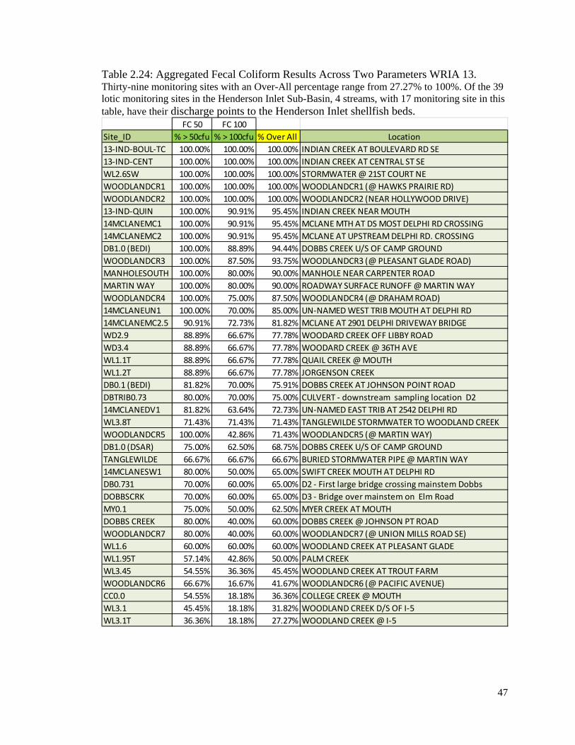
47

Table 2.24: Aggregated Fecal Coliform Results Across Two Parameters WRIA 13. Thirty-nine monitoring sites with an Over-All percentage range from 27.27% to 100%. Of the 39 lotic monitoring sites in the Henderson Inlet Sub-Basin, 4 streams, with 17 monitoring site in this table, have their discharge points to the Henderson Inlet shellfish beds.

FC 50 FC 100Site_ID % > 50cfu % > 100cfu % Over All Location13-IND-BOUL-TC 100.00% 100.00% 100.00% INDIAN CREEK AT BOULEVARD RD SE13-IND-CENT 100.00% 100.00% 100.00% INDIAN CREEK AT CENTRAL ST SEWL2.6SW 100.00% 100.00% 100.00% STORMWATER @ 21ST COURT NEWOODLANDCR1 100.00% 100.00% 100.00% WOODLANDCR1 (@ HAWKS PRAIRIE RD)WOODLANDCR2 100.00% 100.00% 100.00% WOODLANDCR2 (NEAR HOLLYWOOD DRIVE)13-IND-QUIN 100.00% 90.91% 95.45% INDIAN CREEK NEAR MOUTH14MCLANEMC1 100.00% 90.91% 95.45% MCLANE MTH AT DS MOST DELPHI RD CROSSING14MCLANEMC2 100.00% 90.91% 95.45% MCLANE AT UPSTREAM DELPHI RD. CROSSINGDB1.0 (BEDI) 100.00% 88.89% 94.44% DOBBS CREEK U/S OF CAMP GROUNDWOODLANDCR3 100.00% 87.50% 93.75% WOODLANDCR3 (@ PLEASANT GLADE ROAD)MANHOLESOUTH 100.00% 80.00% 90.00% MANHOLE NEAR CARPENTER ROADMARTIN WAY 100.00% 80.00% 90.00% ROADWAY SURFACE RUNOFF @ MARTIN WAYWOODLANDCR4 100.00% 75.00% 87.50% WOODLANDCR4 (@ DRAHAM ROAD)14MCLANEUN1 100.00% 70.00% 85.00% UN-NAMED WEST TRIB MOUTH AT DELPHI RD14MCLANEMC2.5 90.91% 72.73% 81.82% MCLANE AT 2901 DELPHI DRIVEWAY BRIDGEWD2.9 88.89% 66.67% 77.78% WOODARD CREEK OFF LIBBY ROADWD3.4 88.89% 66.67% 77.78% WOODARD CREEK @ 36TH AVEWL1.1T 88.89% 66.67% 77.78% QUAIL CREEK @ MOUTHWL1.2T 88.89% 66.67% 77.78% JORGENSON CREEKDB0.1 (BEDI) 81.82% 70.00% 75.91% DOBBS CREEK AT JOHNSON POINT ROADDBTRIB0.73 80.00% 70.00% 75.00% CULVERT - downstream sampling location D214MCLANEDV1 81.82% 63.64% 72.73% UN-NAMED EAST TRIB AT 2542 DELPHI RDWL3.8T 71.43% 71.43% 71.43% TANGLEWILDE STORMWATER TO WOODLAND CREEKWOODLANDCR5 100.00% 42.86% 71.43% WOODLANDCR5 (@ MARTIN WAY)DB1.0 (DSAR) 75.00% 62.50% 68.75% DOBBS CREEK U/S OF CAMP GROUNDTANGLEWILDE 66.67% 66.67% 66.67% BURIED STORMWATER PIPE @ MARTIN WAY14MCLANESW1 80.00% 50.00% 65.00% SWIFT CREEK MOUTH AT DELPHI RDDB0.731 70.00% 60.00% 65.00% D2 - First large bridge crossing mainstem DobbsDOBBSCRK 70.00% 60.00% 65.00% D3 - Bridge over mainstem on Elm RoadMY0.1 75.00% 50.00% 62.50% MYER CREEK AT MOUTHDOBBS CREEK 80.00% 40.00% 60.00% DOBBS CREEK @ JOHNSON PT ROADWOODLANDCR7 80.00% 40.00% 60.00% WOODLANDCR7 (@ UNION MILLS ROAD SE)WL1.6 60.00% 60.00% 60.00% WOODLAND CREEK AT PLEASANT GLADEWL1.95T 57.14% 42.86% 50.00% PALM CREEKWL3.45 54.55% 36.36% 45.45% WOODLAND CREEK AT TROUT FARMWOODLANDCR6 66.67% 16.67% 41.67% WOODLANDCR6 (@ PACIFIC AVENUE)CC0.0 54.55% 18.18% 36.36% COLLEGE CREEK @ MOUTHWL3.1 45.45% 18.18% 31.82% WOODLAND CREEK D/S OF I-5WL3.1T 36.36% 18.18% 27.27% WOODLAND CREEK @ I-5

48

Chapter Three:

Anthropogenic Land Use and Impervious Surfaces Adjacent to Salmon Habitat and

Shellfish Beds

Introduction:

Human development has altered landscapes and ecosystems in a variety of ways.

These impacts can, and do, alter ecosystem habitats that have been evolving for

thousands of years. Species have been able to adapt to environmental stressors over long

periods of time, but many species struggle to adapt to the rapid growth of the human

impact and hydrological alteration of their ecosystem habitats.

Different types of Land use can affect aquatic systems in many ways, by nutrient

loading that can cause eutrophication, toxic algal blooms, the depletion of dissolved

oxygen and contaminate loading which can affect plant and aquatic species diversity and

abundance. Nutrient loading can come in the form of fertilizers used on lawns and

gardens by urban areas residents, or the runoff from agricultural farms. Residential

wastewater treatment failure of septic systems or leaky sewage treatment lines not only

adds to nutrient loading, but can also increase pathogenic health risks in recreational

waterways. Residential areas, whether urban or rural, generate a lot of waste. Landfills

contain the castoffs of products, broken or unwanted, many which have been

manufactured with harmful toxic chemicals. Plastic packaging and other plastic products

containing phthalates find their way into dump sites, roadway ditches, empty lots, the

gullets of seabirds and even all the way to the large plastic floating island the size of

Texas in the middle of the Pacific Ocean.

Contaminants come in many forms from highly toxic to cloudy water due to

suspended solids. These can affect aquatic species in many ways by making water too

turbid for invertebrate habitation, changing the pH balance, subjecting biota to lethal or

sub-lethal doses of pesticides and herbicides, and mutation and reproductive issues from

endocrine disrupting chemicals and pharmaceuticals.

49

Natural Systems vs. Developed Systems:

The pristine environment provides near ideal solutions for storm water runoff and

pollution control. As rainwater infiltrates into the ground, it is treated by plants and

organisms and is filtered, cleaned, taken up and utilized to sustain life, and returned to the

atmosphere through evapotranspiration. When the infiltrated ground is saturated, excess

rainwater runs off into naturally occurring channels, from creeks to streams to rivers, and

is ultimately returned to the ocean, where it evaporates and begins the hydrologic cycle

all over again in the form of clouds and rain. Each stage of the hydrologic cycle provides

benefits to plants that give us air to breath and even some plants used for food crops.

Mammal and aquatic species also gain benefit from this natural occurring system for

sustenance and suitable habitats. This entire ecosystem service is provided to us all free

of charge, yet we spend a lot of time and money to change and control it.

It has been known for some time now that human development has altered

landscapes and ecosystems in a variety of ways. A Google Scholar ™ search on the

words “Anthropogenic Impact” quickly yields about 142,000 articles on the subject.

Adding to that search the words “…Water Quality,” produces over 84,000 articles. These

published sources demonstrate our awareness of the effect we have on habitat and

species, from the activities we engage in on land and water. These impacts can and do

alter ecosystem habitats that have been long established and evolved for thousands of

years, long before humans set foot on these shores. Species struggle to adapt with the

rapid growth of human impact and hydrological alteration of those ecosystems. We have

become aware of the problems brought on by our presence, yet the question remains,

“How do we fix those problems?” This is fundamentally not an easy question to answer!

Many scientists, biologists, academia, student and volunteer groups seek to understand

ecosystem function, in the hopes of solving at least some of the distress imposed upon

species and habitat. People will continue to build and develop urban areas, as well as

create new urban areas in pristine ecosystems, so the idea is not to inhibit this growth and

development, but rather to find solutions that reduce our impervious footprint, toxic

contamination and nutrient loading and to help us grow and develop in smarter ways to

reduce the effect of our existence.

50

What ever is deposited on the land and infiltrates into the ground will eventually

make its way into drainage ditches, creeks, streams, rivers and ultimately to the estuaries

and oceans. What we do on land can and does effect marine ecosystems. One example is

how bacteria and pathogens flowing downstream to discharge points in the estuaries that

host shellfish beds. Referring to Table 1.2 from the Washington State surface water

quality standards in chapter one, the one parameter in this water analysis for bacteria

levels does not pertain to salmonids and their habitat as much as it does for the protection

of shellfish beds and recreational use. In this thesis fecal coliform data, which is a by-

product of human and other mammal excretion, were used for analysis. The point sources

of fecal coliform contamination are from failure in septic and wastewater systems,

domestic pets and wildlife, farm animals and agriculture. This can result in the discharge

of pathogens from land use to shellfish beds.

Land Use and Estuarine Habitats:

The focus of the following literature review is the anthropogenic impact on

shellfish beds in the Puget Sound, although studies outside this area were also used to

help develop an understanding of how humans affect estuarine habitats. Stressors to a

variety of shellfish species have impacts that depend on the proximity to anthropogenic

changes to the ecosystem, and the needs of specific species to propagate and remain

productive. According to Dr. Megan N. Dethier (2006), the “human effects on habitat

attributes” are defined as: “direct loss of habitat; alteration of substrate type; pollution or

other alterations in nearshore characteristics; alteration of runoff from land and beach

porewater; changes in nearshore plankton, introduced species; increased susceptibility to

predators and parasites;” and “nearshore aquaculture.” The relationship between human

nearshore development and bacteriological quality of water samples taken from their

respective watersheds was also studied. It was found that there is a significant

demographic and land use association with an abundance of fecal coliform in a populated

watershed. Turbidity, which could be caused by anthropogenic activities, was also found

to be related with bacterial abundance. The higher levels of bacteria found in these

estuarine systems can have an increased health risk to humans (Mallen, et al., 2000).

Shellfish play an important role in filtration of nutrients and toxins that run off nearshore

51

lands, which makes them a valuable indicator species for monitoring land use and

evaluating the quality of water that runs off that land and into our estuaries and oceans.

Ultimately the quality and quantity of nutrients, microorganisms, and toxins that are

taken up by shellfish, and then recreationally and commercially harvested, are returned

for human consumption.

Threats to Puget Sound Shellfish:

Shellfish survival and productivity can come under threat in a number of ways.

The most obvious may be from over-harvest by recreational or commercial methods.

Less apparent are those due to alterations of primary ecosystem functions from human

activity and development. Because each shellfish species has distinctive habitat

requirements, for example, sediment type for growth and recruitment, alterations to these

habitats can have a negative impact on shellfish population and productivity. Different

species have preference to different substrate types. Any process, natural or

anthropogenic, that alters substrate habitats by amount of sediment loading, organic

material, and grain size can have a negative effect on shellfish populations. Changes in

river and stream runoff from the land can alter the sediment loads on shellfish beds

(Dethier, 2006). For example, these changes can be sourced by upstream erosion,

landslides or disturbances caused by development, agriculture or logging.

Key parameters according to Dr. Megan N. Dethier (2006) are temperature,

turbidity, salinity, dissolved oxygen, [toxins], pollutants, and food type, all of which can

be affected by land use and shoreline modification. These parameters need to remain at

optimal levels for shellfish to remain productive. When physical conditions of a habitat

deteriorate by anoxic water or excessive sediment, this will place pressures on

productivity. Geoduck juveniles have some mobility for avoiding poor conditions, but the

adults are immobile and subject to higher mortality. Geoduck habitats have been

destroyed by marine construction, and aquaculture projects have competed for their space

(Goodwin & Pease, 1989). Littleneck clams in the larval stage can be affected not only

by salinity and temperature, but high turbidity can reduce their survival rate. High

siltation in their habitats can smother their populations. Dredging nearby or upland

development adds silt to the water columns that will settle upon habitat substrates. The

52

littleneck clams have also been known to be very susceptible to high concentrations of

copper from paint used on boat bottoms (Dethier, 2006).

Impact of Development and Fecal Coliform:

Over a four year period, Michael Mallin (2000) and his research team produced a

study to analyze the distribution and abundance of enteric pathogens in estuaries near

population demographics and development. Their report suggests that nearshore

development poses an increased health risk to humans and has significant consequences

to the environment. The research was performed in the Chesapeake Bay area, but the

fundamentals could apply anywhere there is nearshore development.

Mallin et al., (2000) found a significant correlation between the abundance of

bacteria and turbidity, and fecal coliform bacteria associated with suspended solids in the

water column. This suggests that suspended sediments are a transport mechanism for

fecal bacteria in aquatic systems. Fecal bacteria are known to survive longer in

association with particles of sediment, and disturbance of these sediments can re-release

the fecal bacteria into the water (Mallen, et al., 2000). This occurs with disturbances such

as storm event erosion or clearing land for development.

Input of bacteria into coastal water can have either point or nonpoint sources.

Most point sources can come from failing septic systems and occasionally from leaky

sewer mains or wastewater treatment failures. Nonpoint inputs can vary depending on

land use and demographics. Research by Michael Mallin (2000) revealed a significant

relationship between bacterial loading in the estuaries and watershed population size. He

states that a likely important source of bacterial loading is population. More humans

mean more domesticated animals, which leads to more fecal bacteria deposited on the

land. Also, population size was significantly correlated with the area of estuarine closures

to shellfish beds. The consequence of this is the economic loss to the local community

(Mallen, et al., 2000; Maiolo and Tschtter, 1981).

As it turns out, this study reveals that the percent of impervious surfaces in a

watershed is the most important anthropogenic aspect that contributes to fecal coliform

loads. The impervious surfaces taken into account here are parking lots, driveways, roads,

53

sidewalks and roof tops. Impervious surfaces tend to concentrate and rapidly pass on

storm water that picks up and concentrates pollutants as it rushes to streams and rivers on

its way to the awaiting shellfish in the estuary. A linear regression analysis was

performed and indicated that the area of impervious surfaces alone explained 95% of

variability in average fecal coliform abundance in estuaries, suggesting that urban coastal

areas can reduce their environmental impact by land use practices that reduce impervious

surface area. Methods for doing this include incorporating bioswales, raingardens, and

constructed wetlands into development (Mallen, et al., 2000).

Reports and Surveys:

In order to get a graphic understanding of the relationship between land use and

nearshore habitats specific to shellfish, spatial and tabular data were acquired from the

Washington State Department of Health (DOH) and tabular data from the Washington

State Department of Ecology (DOE). The spatial data from DOH represents commercial

growing areas for shellfish in Western Washington including Puget Sound, and marine

water sampling stations in nearshore habitats. Tabular data from DOE represents water

quality sample stations and results from surface water samples taken at those sites.

Classifications:

Shoreline surveys for the Department of Health had evaluated the drainage system

discharges, agricultural activities, on-site sewage systems as well as wastewater treatment

plants, which could have potential adverse effect on the classification of commercial

shellfish growing areas. The actual and possible pollution sources were defined in these

reports according to the following categories (taken verbatim from the Shoreline Surveys

of Berbells (2003 & 2007) and Zabel-Linclon (2005)):

Direct Impact – A “Direct Impact” is a pollution source that is defined by the National Shellfish Sanitation Program (NSSP) as any waste discharge that has an immediate adverse effect on the growing area.

Indirect Impact – An “Indirect Impact” is a pollution source that is defined by the NSSP as any waste discharge that reaches the growing area in a roundabout way.

54

Potential Source – A “Potential Source” is a pollution source that may influence the water quality in the area. Inadequate setbacks, neglect or abuse of sewage disposal systems, overgrazed pastures and a large number of wildlife are examples that could cause a site to be identified as a potential source of contamination.

No Impact – “No Impact” means the potential source is managed via proper on-site practices or treatment methods so that there is no negative impact on water quality.

Segments of the shellfish growing areas are presently “classified as APPROVED, RESTRICTED, UNCLASSIFIED, OR PROHIBITED” which is based on the identification of pollution source and water quality (Zabel-Linclon, 2005)

The classification of “Conditionally Approved” is in part on wastewater treatment

plant disruptions, but primarily based on rainfall events. A rainfall event that is equal to

or greater than one inch during a 24-hours period will have an imposed restriction to

commercial shellfish harvest for a period of five days. This is true for entire growing

areas classified as conditionally approved (Berbells, 2003). The reasoning behind the five

day wait to lift the restriction on a conditionally approved site after a rainfall event was

revealed during an informational interview with Lawrence Sullivan from the DOH. A

heavy rainfall event will wash contaminates into storm drains, ditches, streams and river

channels. Bacteria are DOH’s contamination of concern, for public health reasons.

Surface water runs off the land and into estuaries where the shellfish are waiting to filter

whatever comes their way. The five day wait period is broken down as, three days for the

bacteria to clean out of the bay to return to a good water quality. Two days after that for

the shellfish to flush out and start taking in water that meets standards.

Criteria:

Shellfish growing areas are classified based on meeting criteria levels for bacteria.

The water samples are taken over a period of time, once a month until approximately 30

samples have been taken. Then these samples are tested for fecal coliform and the results

(organisms/100ml) are recorded. The results are statistically tested for geometric mean

and 90th percentile. The approved standard for shellfish growing waters is stated as: the

55

geometric mean is “not greater than 14 organisms/100ml,” and a “90th percentile not

greater than 43 organisms/100ml (Berbells, 2003 & 2007; Zabel-Linclon, 2005).

Study Areas:

Two areas were selected in South Puget Sound to highlight how human activities

and development have affected commercial shellfish growing areas. The selected areas

were picked for various reasons. One is a wildlife preserve (Nisqually Wildlife Refuge)

that is influenced by activities in its upper watershed; another one is subject to

wastewater treatment, and an area that has been listed with the Department of Ecology as

a 303d for not meeting water quality standards (Henderson Inlet). The reports from DOH

cover the Sanitary Survey and Shoreline Survey for each of these areas.

Description of Growing Area: (As described in reports)

Nisqually Reach: The Nisqually Reach shellfish area is located in southern Puget Sound in Thurston County. The area extends from Johnson Point at the northwest to Dupont at the southeast. The Nisqually River, which is the largest river in the southern Puget Sound, discharges into the southeast end of the area. The total area of the Nisqually Reach shellfish area, including all “Approved”, “Restricted”, “Prohibited”, and “Unclassified” areas, is approximately 4380 acres. Within this area there are approximately 2800 acres classified as “Approved”. A marina closure zone, classified as “Prohibited”, occupies an area of approximately 80 acres located at Baird Cove. Approximately 190 acres between Mill Bight and Puget Marina are “Unclassified”. Fifty acres of shellfish beds located immediately north of the mouth of McAllister Creek are classified as “Restricted”, and approximately 1500 acres of the Nisqually River delta located east and west of the river mouth are classified as “Prohibited” (Melvin, 2006).

The Nisqually Reach shellfish area is located in southern Puget Sound approximately nine miles east of Olympia.” . . . “Oysters, clams, and geoducks are harvested commercially from the area. Most of the intertidal oyster and clam harvest takes place on shellfish beds located at the western edge of the Nisqually River delta. Subtidal commercial geoduck beds are located along the entire length of the area. The majority of the area is classified as “Approved” for commercial shellfish harvest (Melvin, 2006).

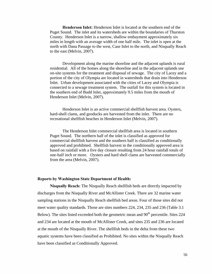
56

Henderson Inlet: Henderson Inlet is located at the southern end of the Puget Sound. The inlet and its watersheds are within the boundaries of Thurston County. Henderson Inlet is a narrow, shallow embayment approximately six miles in length with an average width of one half mile. The inlet is open at the north with Dana Passage to the west, Case Inlet to the north, and Nisqually Reach to the east (Melvin, 2007).

Development along the marine shoreline and the adjacent uplands is rural residential. All of the homes along the shoreline and in the adjacent uplands use on-site systems for the treatment and disposal of sewage. The city of Lacey and a portion of the city of Olympia are located in watersheds that drain into Henderson Inlet. Urban development associated with the cities of Lacey and Olympia is connected to a sewage treatment system. The outfall for this system is located in the southern end of Budd Inlet, approximately 9.5 miles from the mouth of Henderson Inlet (Melvin, 2007).

Henderson Inlet is an active commercial shellfish harvest area. Oysters, hard-shell clams, and geoducks are harvested from the inlet. There are no recreational shellfish beaches in Henderson Inlet (Melvin, 2007).

The Henderson Inlet commercial shellfish area is located in southern Puget Sound. The northern half of the inlet is classified as approved for commercial shellfish harvest and the southern half is classified as conditionally approved and prohibited. Shellfish harvest in the conditionally approved area is based on rainfall with a five day closure resulting from 24 hour rainfall totals of one-half inch or more. Oysters and hard shell clams are harvested commercially from the area (Melvin, 2007).

Reports by Washington State Department of Health:

Nisqually Reach: The Nisqually Reach shellfish beds are directly impacted by

discharges from the Nisqually River and McAllister Creek. There are 32 marine water

sampling stations in the Nisqually Reach shellfish bed areas. Four of those sites did not

meet water quality standards. Those are sites numbers 224, 234, 235 and 236 (Table 3.1

Below). The sites listed exceeded both the geometric mean and 90th percentile. Sites 224

and 234 are located at the mouth of McAllister Creek, and sites 235 and 236 are located

at the mouth of the Nisqually River. The shellfish beds in the delta from these two

aquatic systems have been classified as Prohibited. No sites within the Nisqually Reach

have been classified as Conditionally Approved.

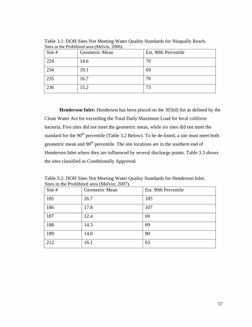
57

Table 3.1: DOH Sites Not Meeting Water Quality Standards for Nisqually Reach. Sites in the Prohibited area (Melvin, 2006).

Henderson Inlet: Henderson has been placed on the 303(d) list as defined by the

Clean Water Act for exceeding the Total Daily Maximum Load for fecal coliform

bacteria. Five sites did not meet the geometric mean, while six sites did not meet the

standard for the 90th percentile (Table 3.2 Below). To be de-listed, a site must meet both

geometric mean and 90th percentile. The site locations are in the southern end of

Henderson Inlet where they are influenced by several discharge points. Table 3.3 shows

the sites classified as Conditionally Approved.

Table 3.2: DOH Sites Not Meeting Water Quality Standards for Henderson Inlet. Sites in the Prohibited area (Melvin, 2007). Site # Geometric Mean Est. 90th Percentile

185 26.7 185

186 17.8 107

187 12.4 69

188 14.3 89

189 14.0 80

212 16.1 63

Site # Geometric Mean Est. 90th Percentile

224 14.6 70

234 19.1 69

235 16.7 70

236 15.2 73

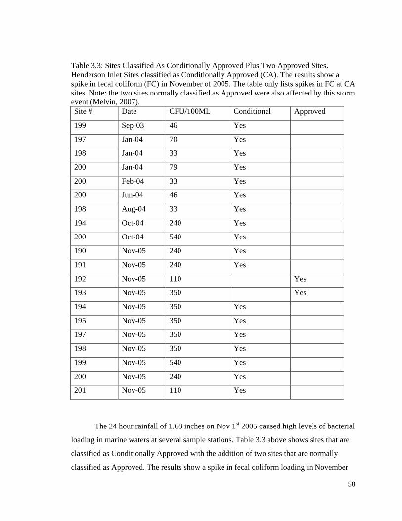
58

Table 3.3: Sites Classified As Conditionally Approved Plus Two Approved Sites. Henderson Inlet Sites classified as Conditionally Approved (CA). The results show a spike in fecal coliform (FC) in November of 2005. The table only lists spikes in FC at CA sites. Note: the two sites normally classified as Approved were also affected by this storm event (Melvin, 2007). Site # Date CFU/100ML Conditional Approved

199 Sep-03 46 Yes

197 Jan-04 70 Yes

198 Jan-04 33 Yes

200 Jan-04 79 Yes

200 Feb-04 33 Yes

200 Jun-04 46 Yes

198 Aug-04 33 Yes

194 Oct-04 240 Yes

200 Oct-04 540 Yes

190 Nov-05 240 Yes

191 Nov-05 240 Yes

192 Nov-05 110 Yes

193 Nov-05 350 Yes

194 Nov-05 350 Yes

195 Nov-05 350 Yes

197 Nov-05 350 Yes

198 Nov-05 350 Yes

199 Nov-05 540 Yes

200 Nov-05 240 Yes

201 Nov-05 110 Yes

The 24 hour rainfall of 1.68 inches on Nov 1st 2005 caused high levels of bacterial

loading in marine waters at several sample stations. Table 3.3 above shows sites that are

classified as Conditionally Approved with the addition of two sites that are normally

classified as Approved. The results show a spike in fecal coliform loading in November

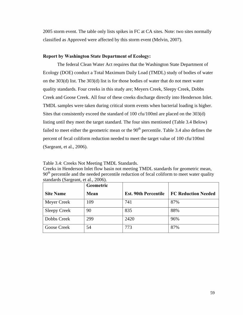
59

2005 storm event. The table only lists spikes in FC at CA sites. Note: two sites normally

classified as Approved were affected by this storm event (Melvin, 2007).

Report by Washington State Department of Ecology:

The federal Clean Water Act requires that the Washington State Department of

Ecology (DOE) conduct a Total Maximum Daily Load (TMDL) study of bodies of water

on the 303(d) list. The 303(d) list is for those bodies of water that do not meet water

quality standards. Four creeks in this study are; Meyers Creek, Sleepy Creek, Dobbs

Creek and Goose Creek. All four of these creeks discharge directly into Henderson Inlet.

TMDL samples were taken during critical storm events when bacterial loading is higher.

Sites that consistently exceed the standard of 100 cfu/100ml are placed on the 303(d)

listing until they meet the target standard. The four sites mentioned (Table 3.4 Below)

failed to meet either the geometric mean or the 90th percentile. Table 3.4 also defines the

percent of fecal coliform reduction needed to meet the target value of 100 cfu/100ml

(Sargeant, et al., 2006).

Table 3.4: Creeks Not Meeting TMDL Standards. Creeks in Henderson Inlet flow basin not meeting TMDL standards for geometric mean, 90th percentile and the needed percentile reduction of fecal coliform to meet water quality standards (Sargeant, et al., 2006).

Site Name

Geometric

Mean Est. 90th Percentile FC Reduction Needed

Meyer Creek 109 741 87%

Sleepy Creek 90 835 88%

Dobbs Creek 299 2420 96%

Goose Creek 54 773 87%

60

Land Use:

The need to define land use increased with population size. Thousands of years

ago indigenous people lived with nature and within its natural cycles. Some peoples were

nomadic as they searched for the things they needed to survive and to be productive.

Some peoples found lands that supplied their every need and they tended to stay more

localized. Whatever the productive strategies of humans were, it was successful and

populations grew. As populations developed in more localized areas, mainly for the

availability of resources, the need to define how the land was used and by who increased.

With increased populations, it became necessary to draw judicial boundaries and

enforce resource management practices. You could do certain activities on your own

property, but your activities were regulated by how they affected your neighbors. With

the need to provide food, water, energy and shelter for a growing population,

environmental issues were generally considered local. With the worldwide changes to

farmland, forests and waterways now upon us, this leaves us facing many challenges to

manage trade-offs in sharing the planet’s resources (Foley, et al., 2005).

Our ancient ancestors lived at a time when ecosystems were mostly pristine and

their impact on the environment was minimal. With the large populations of today, our

impact on the environment is being felt, and many of the disposable products of modern

society are coming back to haunt us. Even hundreds of years ago we could throw

something away and this wonderful planet we lived on would just absorb it. But now we

are discovering that there is no place called “Away.” Our ecosystems have become so

impacted by our activities and our byproducts that those things we thought we could

throw away are now revisiting us through our food, air and water.

Never before in our long human history has it been so important that we change

our thinking on how we use the land we have been given. October 31st 2011 was the day

set by the United Nation’s Demographers when it was stated that the world human

population would hit 7 Billion (Biello, 2011). Our large population has surpassed our

carrying capacity and we face an increased need to share global resources. We have

overseen an incredible loss of biodiversity and increase of pollution to air and water

(Foley, et al., 2005). Our land use problem is two-fold. We need to identify and fix the

61

errors of past land use practices, and also change the way we use our land in order to

minimize our ecological footprint upon it.

Land Use Types: Anthropogenic land use has an effect on the quality of runoff

water from different types of land uses such as urban, commercial, agriculture, industrial,

forestry and recreational. With increasing population and the need for urban and

industrial development, the burden of our environmental footprint increases. River

systems and the watersheds that supply them with runoff water have had their hydrology

altered by increased development. More urban development means more impervious

surfaces. A study by Park et al. (2007) used LANDSAT data to show that land use is a

significant factor in the contribution of pollutant loading. Impervious surfaces and current

stormwater management systems contribute to rapid storm surge into streams and rivers

that normally reach capacity during heavy storm events. Along with impervious surfaces,

the system of creeks and streams that have been channelized into long straight ditches

contribute to storm surge. The purpose of these ditches is to quickly remove runoff water

from developed locations, to prevent water from ponding on property and agricultural

fields. The problem with channelization is the destruction of habitat, undercutting roads

and utilities, increase in non-point pollution, contributions to flooding downstream, and

the devaluation of property in those flood prone areas (US EPA, Date Unknown).

WRIA 11 Parcels: The boundary for the Nisqually River Basin cuts through

three counties: Thurston, Pierce and Lewis. Parcel data were collected for all three of

those counties and the parcels specific to WRIA 11 were extracted from those data using

GIS procedures. A categorical data method was used on the Nisqually River Basin parcel

data set to create different land use types for calculating area and percent of the overall

land use totals. The categorical information for land use types was taken from the land

use code field in each parcel data set.

All the land use type parcels contained within that boundary cover an area of

483,420.90 acres (100% of all land use types). The dominate land use type in the

Nisqually watershed was determined to be Forest at 264,653.17 acres, or 54.75% of the

total land use. That was followed by land that was Underdeveloped, Undeveloped or

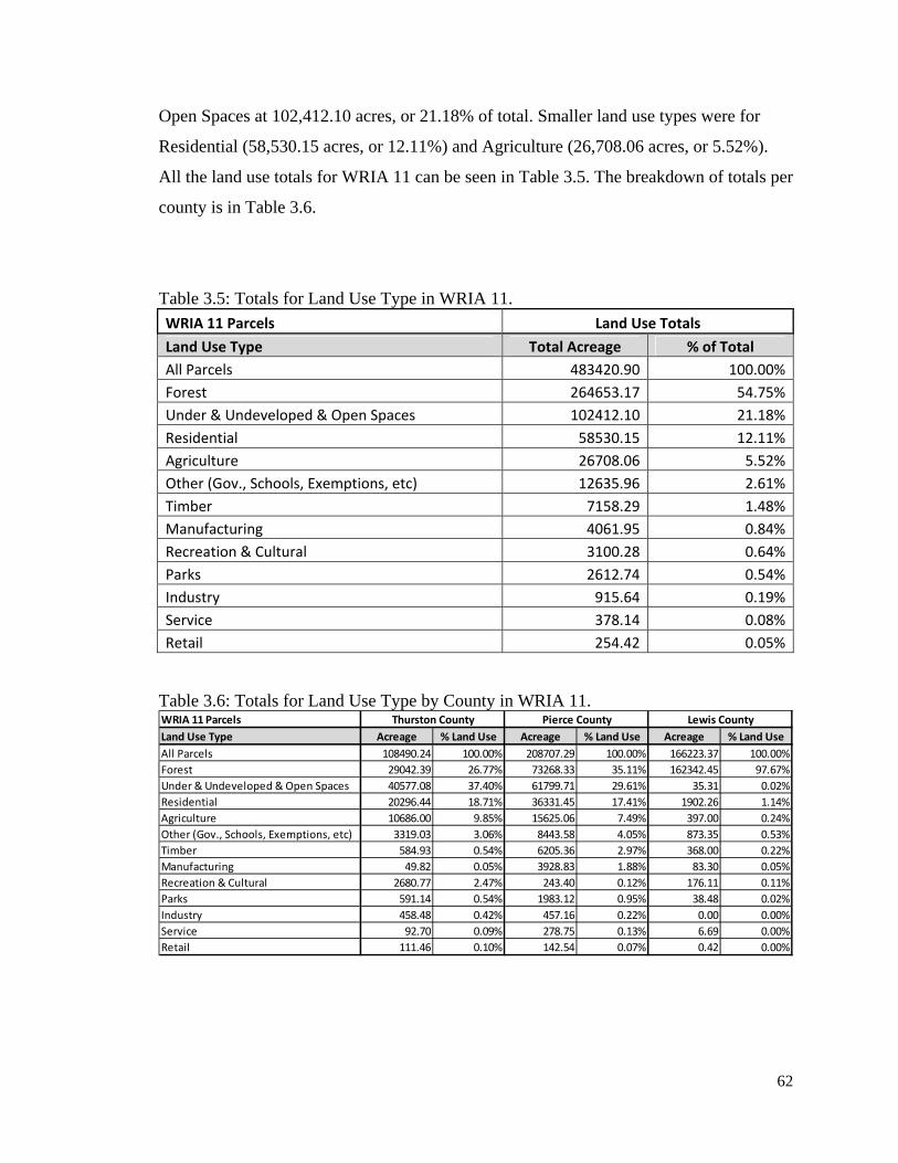
62

Open Spaces at 102,412.10 acres, or 21.18% of total. Smaller land use types were for

Residential (58,530.15 acres, or 12.11%) and Agriculture (26,708.06 acres, or 5.52%).

All the land use totals for WRIA 11 can be seen in Table 3.5. The breakdown of totals per

county is in Table 3.6.

Table 3.5: Totals for Land Use Type in WRIA 11. WRIA 11 Parcels Land Use Totals

Land Use Type Total Acreage % of Total All Parcels 483420.90 100.00%Forest 264653.17 54.75%Under & Undeveloped & Open Spaces 102412.10 21.18%Residential 58530.15 12.11%Agriculture 26708.06 5.52%Other (Gov., Schools, Exemptions, etc) 12635.96 2.61%Timber 7158.29 1.48%Manufacturing 4061.95 0.84%Recreation & Cultural 3100.28 0.64%Parks 2612.74 0.54%Industry 915.64 0.19%Service 378.14 0.08%Retail 254.42 0.05%

Table 3.6: Totals for Land Use Type by County in WRIA 11. WRIA 11 ParcelsLand Use Type Acreage % Land Use Acreage % Land Use Acreage % Land UseAll Parcels 108490.24 100.00% 208707.29 100.00% 166223.37 100.00%Forest 29042.39 26.77% 73268.33 35.11% 162342.45 97.67%Under & Undeveloped & Open Spaces 40577.08 37.40% 61799.71 29.61% 35.31 0.02%Residential 20296.44 18.71% 36331.45 17.41% 1902.26 1.14%Agriculture 10686.00 9.85% 15625.06 7.49% 397.00 0.24%Other (Gov., Schools, Exemptions, etc) 3319.03 3.06% 8443.58 4.05% 873.35 0.53%Timber 584.93 0.54% 6205.36 2.97% 368.00 0.22%Manufacturing 49.82 0.05% 3928.83 1.88% 83.30 0.05%Recreation & Cultural 2680.77 2.47% 243.40 0.12% 176.11 0.11%Parks 591.14 0.54% 1983.12 0.95% 38.48 0.02%Industry 458.48 0.42% 457.16 0.22% 0.00 0.00%Service 92.70 0.09% 278.75 0.13% 6.69 0.00%Retail 111.46 0.10% 142.54 0.07% 0.42 0.00%

Thurston County Pierce County Lewis County

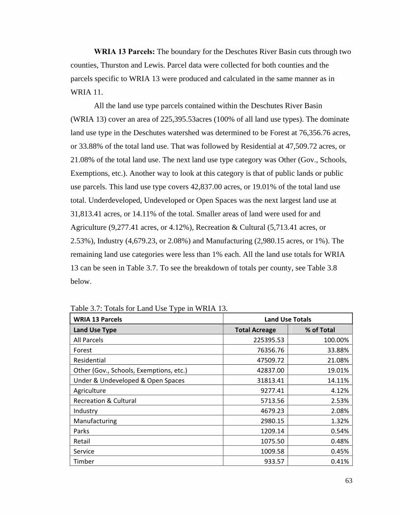
63

WRIA 13 Parcels: The boundary for the Deschutes River Basin cuts through two

counties, Thurston and Lewis. Parcel data were collected for both counties and the

parcels specific to WRIA 13 were produced and calculated in the same manner as in

WRIA 11.

All the land use type parcels contained within the Deschutes River Basin

(WRIA 13) cover an area of 225,395.53acres (100% of all land use types). The dominate

land use type in the Deschutes watershed was determined to be Forest at 76,356.76 acres,

or 33.88% of the total land use. That was followed by Residential at 47,509.72 acres, or

21.08% of the total land use. The next land use type category was Other (Gov., Schools,

Exemptions, etc.). Another way to look at this category is that of public lands or public

use parcels. This land use type covers 42,837.00 acres, or 19.01% of the total land use

total. Underdeveloped, Undeveloped or Open Spaces was the next largest land use at

31,813.41 acres, or 14.11% of the total. Smaller areas of land were used for and

Agriculture (9,277.41 acres, or 4.12%), Recreation & Cultural (5,713.41 acres, or

2.53%), Industry (4,679.23, or 2.08%) and Manufacturing (2,980.15 acres, or 1%). The

remaining land use categories were less than 1% each. All the land use totals for WRIA

13 can be seen in Table 3.7. To see the breakdown of totals per county, see Table 3.8

below.

Table 3.7: Totals for Land Use Type in WRIA 13. WRIA 13 Parcels Land Use Totals

Land Use Type Total Acreage % of Total All Parcels 225395.53 100.00%Forest 76356.76 33.88%Residential 47509.72 21.08%Other (Gov., Schools, Exemptions, etc.) 42837.00 19.01%Under & Undeveloped & Open Spaces 31813.41 14.11%Agriculture 9277.41 4.12%Recreation & Cultural 5713.56 2.53%Industry 4679.23 2.08%Manufacturing 2980.15 1.32%Parks 1209.14 0.54%Retail 1075.50 0.48%Service 1009.58 0.45%Timber 933.57 0.41%

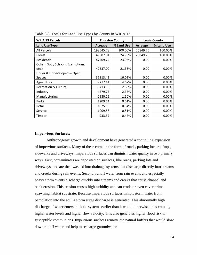
64

Table 3.8: Totals for Land Use Types by County in WRIA 13.

WRIA 13 Parcels Thurston County Lewis County

Land Use Type Acreage % Land Use Acreage % Land Use All Parcels 198545.78 100.00% 26849.75 100.00%Forest 49507.01 24.93% 26849.75 100.00%Residential 47509.72 23.93% 0.00 0.00%Other (Gov., Schools, Exemptions, etc.) 42837.00 21.58% 0.00 0.00%Under & Undeveloped & Open Spaces 31813.41 16.02% 0.00 0.00%Agriculture 9277.41 4.67% 0.00 0.00%Recreation & Cultural 5713.56 2.88% 0.00 0.00%Industry 4679.23 2.36% 0.00 0.00%Manufacturing 2980.15 1.50% 0.00 0.00%Parks 1209.14 0.61% 0.00 0.00%Retail 1075.50 0.54% 0.00 0.00%Service 1009.58 0.51% 0.00 0.00%Timber 933.57 0.47% 0.00 0.00%

Impervious Surfaces:

Anthropogenic growth and development have generated a continuing expansion

of impervious surfaces. Many of these come in the form of roads, parking lots, rooftops,

sidewalks and driveways. Impervious surfaces can diminish water quality in two primary

ways. First, contaminates are deposited on surfaces, like roads, parking lots and

driveways, and are then washed into drainage systems that discharge directly into streams

and creeks during rain events. Second, runoff water from rain events and especially

heavy storm events discharge quickly into streams and creeks that cause channel and

bank erosion. This erosion causes high turbidity and can erode or even cover prime

spawning habitat substrate. Because impervious surfaces inhibit storm water from

percolation into the soil, a storm surge discharge is generated. This abnormally high

discharge of water enters the lotic systems earlier than it would otherwise, thus creating

higher water levels and higher flow velocity. This also generates higher flood risk to

susceptible communities. Impervious surfaces remove the natural buffers that would slow

down runoff water and help to recharge groundwater.

65

We pave over the permeable surfaces, erect huge box stores, build our homes, lay

down roads so we can get from one place to the other, and for our convenience cluster

stores together in large impermeable Mega-Malls, so we can shop from store to store

without having to move our car. These parking lots and malls with huge box stores create

a very large impervious footprint that thwarts the natural hydrological cycle.

The Problem: The built environment comes with external cost for which we have

not accounted. The increasing numbers of buildings, parking lots and roads have created

impervious surfaces that block the natural infiltration of rainwater into the ground. The

urbanization of a watershed has profound effects that degrade downstream habitats, as

well as increase flood frequency and decrease the base flow of a river (Asleson, et al.,

2009). U.S. urban land use is projected to increase from 3.1% in the year 2000 to 8.1% in

2050, an area larger than the state of Montana. The growth in urban land necessitates the

need for more planning and regional management of resources and ecosystem services

for this growing population (Nowak & Walton, 2005). Currently, to deal with the

rainwater not infiltrated into groundwater, we build an infrastructure of ditches and

modify stream channels to more quickly and effectively shed excess surface water away

from buildings and parking lots. As long as we are living on higher ground, it may seem

like a good solution to rapidly remove unwanted water downstream to the river. But,

what of the logic that challenges practical ecological reasoning; the need we have to build

in the river’s flood plain.

We build in flood plains because it is flat, easy and cheaper to build there (seldom

mindful the reason it is called a flood plain). Rivers flood from time to time as part of

their natural cycle. This flooding event replenishes nutrients to habitats for free. Also,

that rich soil is a desirable influence for living and working there. So, we build up the

flood plain with more impervious surfaces, the last place for rainwater to get absorbed

into the ground before reaching the river and ultimately the ocean. The efficient drainage

system created to shed storm water, now adds extra water to the river’s flood stage during

storm events. To protect our need to build in the flood plain, we invest more money to

build dikes and levees to protect our flood plain investment, and dams to hold back runoff

water. Those solutions come at of big cost to economy and ecosystems.

66

Another unexpected consequence of impervious surfaces is the contaminant

deposits upon them that get washed directly into streams and rivers, thus impacting

habitats and the species that occupy aquatic habitats. Our growing population and the

increase of urbanization and industrialization are considered the primary factors

responsible for the increase of pollution of our aquatic systems. These water bodies

receive residential and industrial waste from surface runoff. We now have to build

conventional methods for treating this waste, which are generally costly and not

ecofriendly (Dhote & Dixit, 2009). In contrast, there are systems being developed that

mimic a more natural self-purification, water impoundment and infiltration system. A

study by Scholz & Kazemi Yazdi (2009) showed that runoff water and pollution levels

can be successfully reduced by utilization of storm water detention areas.

With increasing population and the need for urban and industrial development, the

burden of our environmental footprint increases. River systems and the watersheds that

supply them with runoff water have been hydrology altered by this increased

development. More urban development means more impervious surfaces. A study by

Park et al., (2007) used LANDSAT data to show that land use as a significant factor in

the contribution of pollutant loading. Impervious surfaces and current storm water

management systems contribute to rapid storm surge into streams and rivers that

normally reach capacity during heavy storm events. Along with impervious surfaces that

contribute to storm surge are the system of creeks and streams that have been channelized

into long straight ditches. The purpose of these ditches is to quickly remove runoff water

from developed locations, to prevent water from ponding on property and agricultural

fields. The problem with channelization is that it destroys habitat, undercuts roads and

utilities, increases non-point pollution, contributes to flooding downstream, and the

devaluation of property in those flood prone areas (US EPA, Date Unknown).

To sum it up, urban areas are growing, and with this growth we generate a larger

ecological footprint. The question we should be asking ourselves in our quest for

development is, “Do we want the land we build on to inhibit the natural hydrologic cycle,

or do we want it to work with the natural cycles to reduce the negative impact of our

presence upon it?”

67

The effect of urban growth with its impervious surfaces is a big problem to tackle,

and some communities show a growing desire to work with natural system to solve the

problems created by growth. Mallin (2000) suggests low-impact development practices

can solve many of the problems produced by the urban impervious footprint.

Analysis of the Lower Henderson Inlet Sub-Basin Septic Systems as Source of Fecal

Coliform Loading on Shellfish Beds:

The WRIA 13 water quality parameter tabular data analysis, discussed in

Chapter 2, revealed 17 monitoring sites on streams having their discharge points into the

Henderson Inlet shellfish beds. Henderson Inlet sub-basin is divided into an upper and

lower flow basin. The upper basin sheds water from a variety of residential and

commercial land use parcels. This area is drained by two main creek systems, Woodland

Creek and Woodard Creek. Woodland Creek flows north through the residential and

commercial districts of the City of Lacey, and discharges at the southern end of

Henderson Inlet estuary. Woodard Creek flows north and drains parts of east Olympia

and western parts of Lacey, before it discharges into the mid portion of Henderson Inlet

estuary on the west side.

Lower Henderson Inlet basin sheds water from residential, agricultural and forest

land adjacent to the inlet on it west and east banks. Figure 3.1 shows the boundary of the

lower basin in the shaded area on the map and the shellfish beds area. Many of the

residential and agricultural parcels in this area have septic systems for wastewater

treatment. Also, seven of the monitoring sites in this basin failed to meet the analysis

criterion for FC 50 at the 35% plus geometric mean standard. Lower Henderson Inlet

basin was chosen for GIS spatial analysis because of the density of parcels within it with

septic systems. This analysis was set up to identify potential point sources of fecal

coliform bacterial contamination. Upper Henderson Inlet flow basin also contained

parcels on septic systems, but are more spread out. The same methods for spatial analysis

can be used in both upper and lower flow basins. The density of septic systems and the

close proximity to shellfish beds is why the lower flow basin was chosen for this study.

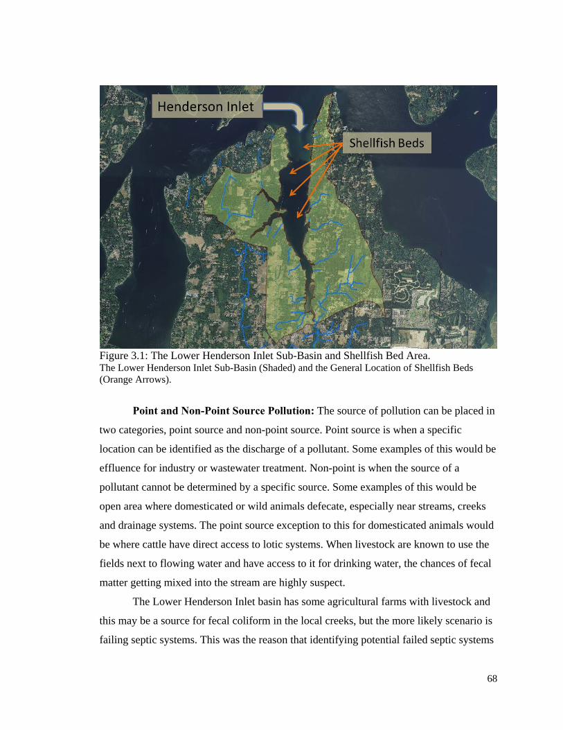
68

Figure 3.1: The Lower Henderson Inlet Sub-Basin and Shellfish Bed Area. The Lower Henderson Inlet Sub-Basin (Shaded) and the General Location of Shellfish Beds (Orange Arrows).

Point and Non-Point Source Pollution: The source of pollution can be placed in

two categories, point source and non-point source. Point source is when a specific

location can be identified as the discharge of a pollutant. Some examples of this would be

effluence for industry or wastewater treatment. Non-point is when the source of a

pollutant cannot be determined by a specific source. Some examples of this would be

open area where domesticated or wild animals defecate, especially near streams, creeks

and drainage systems. The point source exception to this for domesticated animals would

be where cattle have direct access to lotic systems. When livestock are known to use the

fields next to flowing water and have access to it for drinking water, the chances of fecal

matter getting mixed into the stream are highly suspect.

The Lower Henderson Inlet basin has some agricultural farms with livestock and

this may be a source for fecal coliform in the local creeks, but the more likely scenario is

failing septic systems. This was the reason that identifying potential failed septic systems

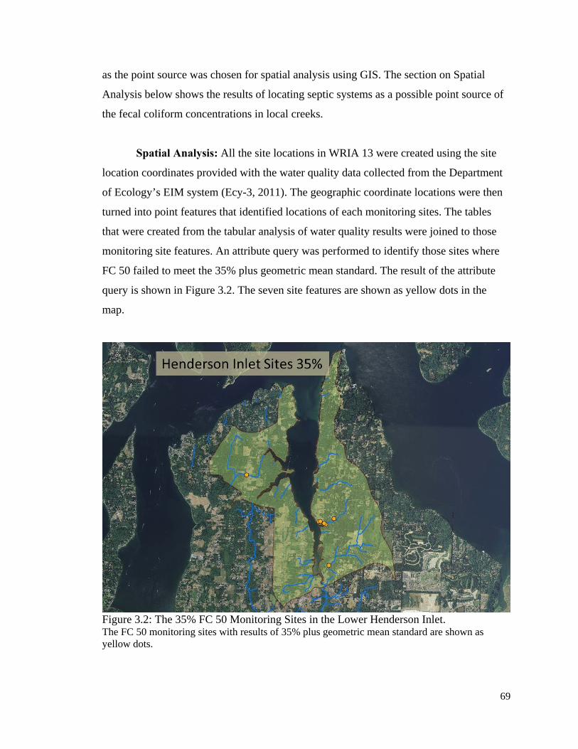
69

as the point source was chosen for spatial analysis using GIS. The section on Spatial

Analysis below shows the results of locating septic systems as a possible point source of

the fecal coliform concentrations in local creeks.

Spatial Analysis: All the site locations in WRIA 13 were created using the site

location coordinates provided with the water quality data collected from the Department

of Ecology’s EIM system (Ecy-3, 2011). The geographic coordinate locations were then

turned into point features that identified locations of each monitoring sites. The tables

that were created from the tabular analysis of water quality results were joined to those

monitoring site features. An attribute query was performed to identify those sites where

FC 50 failed to meet the 35% plus geometric mean standard. The result of the attribute

query is shown in Figure 3.2. The seven site features are shown as yellow dots in the

map.

Figure 3.2: The 35% FC 50 Monitoring Sites in the Lower Henderson Inlet. The FC 50 monitoring sites with results of 35% plus geometric mean standard are shown as yellow dots.

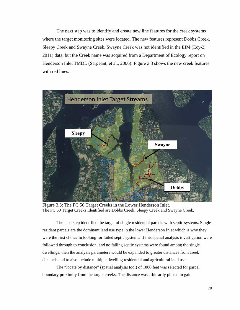
70

The next step was to identify and create new line features for the creek systems

where the target monitoring sites were located. The new features represent Dobbs Creek,

Sleepy Creek and Swayne Creek. Swayne Creek was not identified in the EIM (Ecy-3,

2011) data, but the Creek name was acquired from a Department of Ecology report on

Henderson Inlet TMDL (Sargeant, et al., 2006). Figure 3.3 shows the new creek features

with red lines.

Figure 3.3: The FC 50 Target Creeks in the Lower Henderson Inlet. The FC 50 Target Creeks Identified are Dobbs Creek, Sleepy Creek and Swayne Creek.

The next step identified the target of single residential parcels with septic systems. Single

resident parcels are the dominant land use type in the lower Henderson Inlet which is why they

were the first choice in looking for failed septic systems. If this spatial analysis investigation were

followed through to conclusion, and no failing septic systems were found among the single

dwellings, then the analysis parameters would be expanded to greater distances from creek

channels and to also include multiple dwelling residential and agricultural land use.

The “locate by distance” (spatial analysis tool) of 1000 feet was selected for parcel

boundary proximity from the target creeks. The distance was arbitrarily picked to gain

Dobbs

Swayne

Sleepy

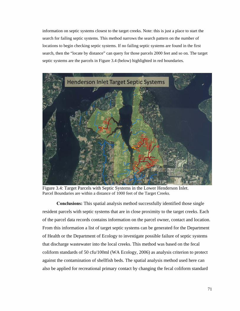
71

information on septic systems closest to the target creeks. Note: this is just a place to start the

search for failing septic systems. This method narrows the search pattern on the number of

locations to begin checking septic systems. If no failing septic systems are found in the first

search, then the “locate by distance” can query for those parcels 2000 feet and so on. The target

septic systems are the parcels in Figure 3.4 (below) highlighted in red boundaries.

Figure 3.4: Target Parcels with Septic Systems in the Lower Henderson Inlet. Parcel Boundaries are within a distance of 1000 feet of the Target Creeks. Conclusions: This spatial analysis method successfully identified those single

resident parcels with septic systems that are in close proximity to the target creeks. Each

of the parcel data records contains information on the parcel owner, contact and location.

From this information a list of target septic systems can be generated for the Department

of Health or the Department of Ecology to investigate possible failure of septic systems

that discharge wastewater into the local creeks. This method was based on the fecal

coliform standards of 50 cfu/100ml (WA Ecology, 2006) as analysis criterion to protect

against the contamination of shellfish beds. The spatial analysis method used here can

also be applied for recreational primary contact by changing the fecal coliform standard

72

to 100 cfu/100ml (WA Ecology, 2006) as the analysis criterion. Review of these water

quality standards can be found in Table 1.2 in Chapter One.

The easiest phase of the identification of parcels with target septic systems was

performed with the GIS software. The majority of the work in this study was the

management of the water quality tabular data. Those data records needed to be proofed

for quality assurance, organized by monitoring sites, algorithms created for each

parameter based on water quality criteria, a tier ranking system defined, ranking results

tables created, aggregation tables created across multiple parameters and ranking tables

prepared as join table for the GIS location features.

The GIS preparation for the Henderson Inlet study needed the acquisition and

creation of spatial layers in part for display purposes and spatial analysis. The layers for

map image display started with an orthophoto (geographically referenced aerial photo) of

Thurston County. On this image were two other layers, a boundary of the lower

Henderson Inlet flow basin and a hydrology layer for the Henderson Inlet basin creeks.

To create a land use layer for the lower Henderson Inlet, Thurston County parcel data

were used (refer to the section on Land Use / WRIA 13 Parcels). The Geoprocessing Clip

tool in ArcGIS® was used to create parcel features for the lower Henderson Inlet flow

basin area. The water quality data downloaded from EIM (Ecy-3. 2011) provided the

coordinates for the location of each monitoring site. The coordinates were converted to

point features in GIS and used to join the ranking tables for analysis. The last layer

needed was the target creeks that were generated from the first phase of the analysis

process. These were turned into a feature for the next phase of identifying target parcels

with septic systems.

This method for identification of target parcels works well with the above

mentioned analysis structure. This method can be easily replicated for other flow basins

where sewer system types are part of the parcel data. Thurston County did include that

type of information, whereas Pierce and Lewis Counties did not. Other sources of data

would need to be obtained if this type of analysis were performed for Pierce or Lewis

Counties.

73

Chapter Four:

Defining Flow Basin Influence on Degraded Lotic Systems

Introduction:

Identifying degraded water quality at specific sampling sites in streams and rivers

is only one part of the picture of degraded habitats. To understand what is influencing the

water quality results at these sample sites, one must also understand the potential

contributing factors to those results. Water flows downhill, therefore the drainage area

above these water quality sampling sites would be the potential influence on the results

acquired from those sample sites. This area is defined as the flow basin to each of those

sample sites. Within those flow basins are different aquatic systems like streams and

creeks, wetlands, as well as forest and many different other land use types.

Flow basins are digitally defined by using ArcGIS® hydrology tools to analyze

digital elevation models (DEM) for flow direction and accumulation. This method can be

used to calculate area for any spatial data flow point; in the case of this thesis those points

represent the water quality sampling sites of interest. The points of interest are sites not

meeting water quality standard for the highest percentage of time sampled. Once the flow

basin is generated, it is used to calculate the different land use types within its boundary.

The different land use types are extracted from parcel layers provided by the counties

represented by watersheds in this study. The parcel information comes from Thurston,

Peirce and Lewis Counties in western Washington State.

Before defining the land use influences, it is important to describe the types of

impacts from anthropogenic activities from those different land uses.

Watershed Function and Stressors:

Watersheds support diverse components of an ecosystem, while providing a

system that purifies water by filtering out pollution, sediments, and toxins. Increased

population, economic activities, and development have put stresses on watersheds by

added pollution and depletion of resources. This anthropogenic activity may well cause a

decline in living standards and destabilize the integrity of the ecosystem. Ranking among

74

the most urgent issues facing us today, by 200 leading scientists from more than 50

countries, sustainable watershed management should receive some of the highest

priorities (Levy et al., 2006).

It should also be noted that flowing aquatic systems like streams, rivers, and even

drainage ditches have not only that which can be seen within their channels, but also

include the unseen system and the not so obvious. A watershed does what it says; it sheds

water and ultimately flows down slope to its lowest point. Watersheds are integrated

systems of water channels, wetlands, runoff, and ground water. Watersheds are also

complex ecosystems that have established equilibrium of plants and animals over

thousands of years. These complex ecosystems cycle nutrients and basic elements

throughout the watershed with the help of down slope movement, runoff from rainfall,

and animals spreading nutrients throughout local and upstream habitats, to just name a

few. Water seen in a channel actually extends beyond its banks as groundwater. If the

water table is high, the ground water flows toward the open stream channel, and if the

water table is low, the water in the channel will saturate the surrounding soils and

replenish the groundwater. Lipophilic organic toxins in stream water can bond with soil.

In low water table conditions, these contaminants can become imbedded in the soils

around the stream banks as water saturates the surrounding soils. In high water table

conditions, and especially during storm events, lipophilic toxins can enter the aquatic

system through soil erosion. Any contaminants deposited on the ground follow along the

same complex system as do the nutrients and elements. This is why it is so important to

have a functional riparian zone along the edge of flowing systems to filter and uptake

contaminants. A riparian zone is nature’s plant and microorganism remediation system.

This is how nature takes care of itself, but what about anthropogenic disturbances to

nature’s filtration system?

Urban development has impacted greatly the health and equilibrium of

watersheds. Urban watersheds should be perceived as integrated physical systems. Their

function is dependent on the interaction of chemicals, ecological elements, and the

hydrology of the system. Urbanization can have a negative impact in a cumulative

manner as drainage systems and smaller streams contribute higher peak flows as well as

heavy sediment and pollutant loads to the higher order waterways downstream. As

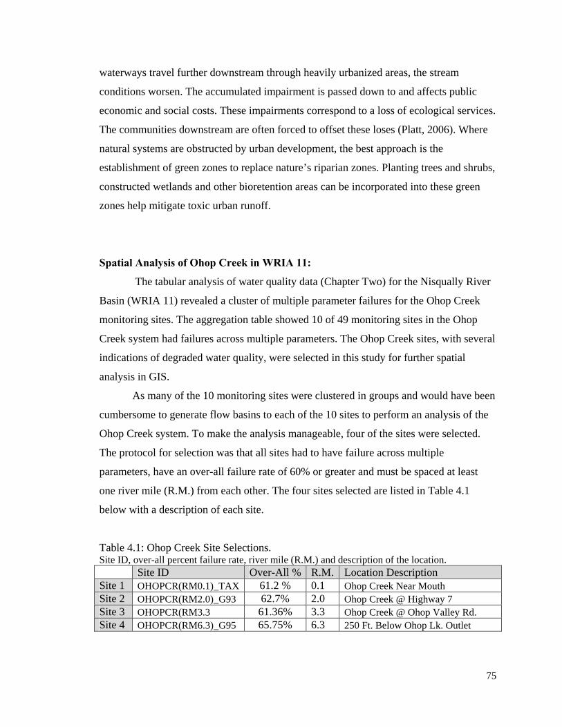
75

waterways travel further downstream through heavily urbanized areas, the stream

conditions worsen. The accumulated impairment is passed down to and affects public

economic and social costs. These impairments correspond to a loss of ecological services.

The communities downstream are often forced to offset these loses (Platt, 2006). Where

natural systems are obstructed by urban development, the best approach is the

establishment of green zones to replace nature’s riparian zones. Planting trees and shrubs,

constructed wetlands and other bioretention areas can be incorporated into these green

zones help mitigate toxic urban runoff.

Spatial Analysis of Ohop Creek in WRIA 11:

The tabular analysis of water quality data (Chapter Two) for the Nisqually River

Basin (WRIA 11) revealed a cluster of multiple parameter failures for the Ohop Creek

monitoring sites. The aggregation table showed 10 of 49 monitoring sites in the Ohop

Creek system had failures across multiple parameters. The Ohop Creek sites, with several

indications of degraded water quality, were selected in this study for further spatial

analysis in GIS.

As many of the 10 monitoring sites were clustered in groups and would have been

cumbersome to generate flow basins to each of the 10 sites to perform an analysis of the

Ohop Creek system. To make the analysis manageable, four of the sites were selected.

The protocol for selection was that all sites had to have failure across multiple

parameters, have an over-all failure rate of 60% or greater and must be spaced at least

one river mile (R.M.) from each other. The four sites selected are listed in Table 4.1

below with a description of each site.

Table 4.1: Ohop Creek Site Selections. Site ID, over-all percent failure rate, river mile (R.M.) and description of the location. Site ID Over-All % R.M. Location Description Site 1 OHOPCR(RM0.1)_TAX 61.2 % 0.1 Ohop Creek Near Mouth Site 2 OHOPCR(RM2.0)_G93 62.7% 2.0 Ohop Creek @ Highway 7 Site 3 OHOPCR(RM3.3 61.36% 3.3 Ohop Creek @ Ohop Valley Rd. Site 4 OHOPCR(RM6.3)_G95 65.75% 6.3 250 Ft. Below Ohop Lk. Outlet

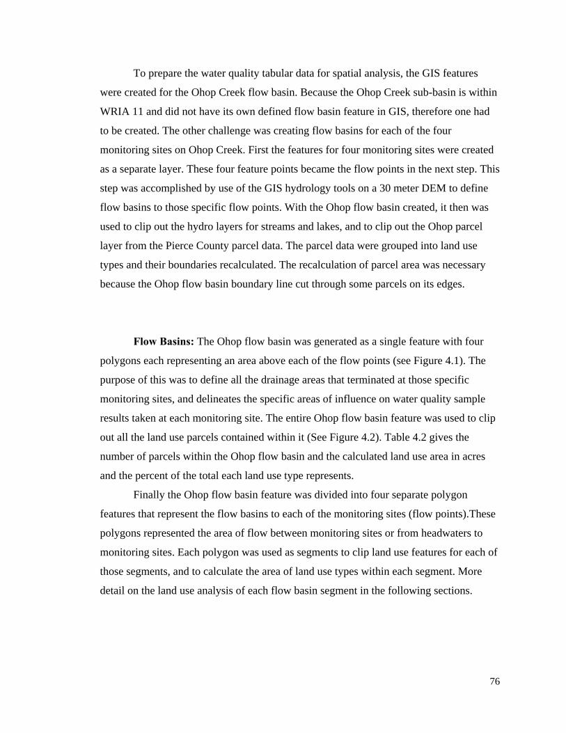
76

To prepare the water quality tabular data for spatial analysis, the GIS features

were created for the Ohop Creek flow basin. Because the Ohop Creek sub-basin is within

WRIA 11 and did not have its own defined flow basin feature in GIS, therefore one had

to be created. The other challenge was creating flow basins for each of the four

monitoring sites on Ohop Creek. First the features for four monitoring sites were created

as a separate layer. These four feature points became the flow points in the next step. This

step was accomplished by use of the GIS hydrology tools on a 30 meter DEM to define

flow basins to those specific flow points. With the Ohop flow basin created, it then was

used to clip out the hydro layers for streams and lakes, and to clip out the Ohop parcel

layer from the Pierce County parcel data. The parcel data were grouped into land use

types and their boundaries recalculated. The recalculation of parcel area was necessary

because the Ohop flow basin boundary line cut through some parcels on its edges.

Flow Basins: The Ohop flow basin was generated as a single feature with four

polygons each representing an area above each of the flow points (see Figure 4.1). The

purpose of this was to define all the drainage areas that terminated at those specific

monitoring sites, and delineates the specific areas of influence on water quality sample

results taken at each monitoring site. The entire Ohop flow basin feature was used to clip

out all the land use parcels contained within it (See Figure 4.2). Table 4.2 gives the

number of parcels within the Ohop flow basin and the calculated land use area in acres

and the percent of the total each land use type represents.

Finally the Ohop flow basin feature was divided into four separate polygon

features that represent the flow basins to each of the monitoring sites (flow points).These

polygons represented the area of flow between monitoring sites or from headwaters to

monitoring sites. Each polygon was used as segments to clip land use features for each of

those segments, and to calculate the area of land use types within each segment. More

detail on the land use analysis of each flow basin segment in the following sections.

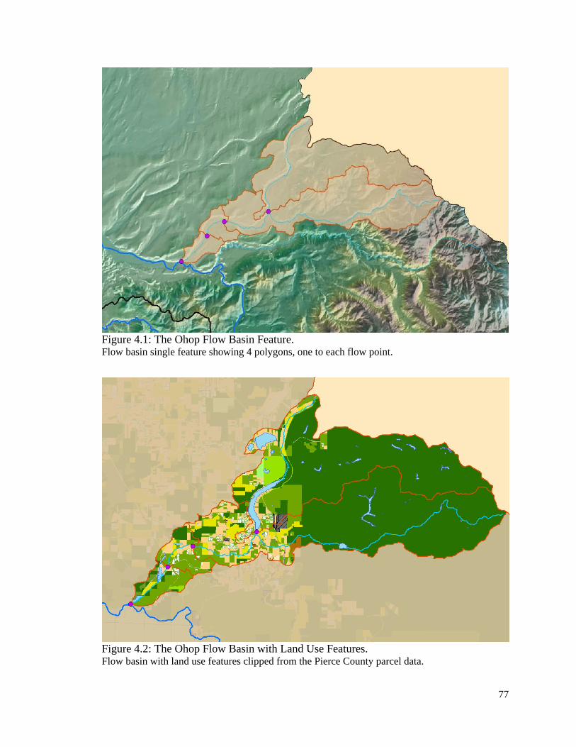
77

Figure 4.1: The Ohop Flow Basin Feature. Flow basin single feature showing 4 polygons, one to each flow point.

Figure 4.2: The Ohop Flow Basin with Land Use Features. Flow basin with land use features clipped from the Pierce County parcel data.

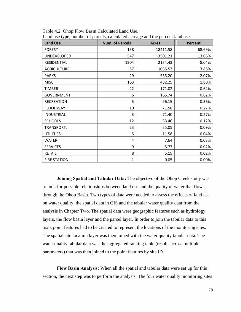
78

Table 4.2: Ohop Flow Basin Calculated Land Use. Land use type, number of parcels, calculated acreage and the percent land use. Land Use Num. of Parcels Acres Percent

FOREST 138 18411.58 68.69%

UNDEVELOPED 547 3501.21 13.06%

RESIDENTIAL 1204 2154.43 8.04%

AGRICULTURE 57 1035.57 3.86%

PARKS 29 555.20 2.07%

MISC. 163 482.25 1.80%

TIMBER 22 171.02 0.64%

GOVERNMENT 6 165.74 0.62%

RECREATION 5 96.15 0.36%

FLOODWAY 10 71.58 0.27%

INDUSTRIAL 3 71.40 0.27%

SCHOOLS 12 33.46 0.12%

TRANSPORT. 23 25.05 0.09%

UTILITIES 5 11.58 0.04%

WATER 4 7.64 0.03%

SERVICES 9 5.77 0.02%

RETAIL 8 5.15 0.02%

FIRE STATION 1 0.05 0.00%

Joining Spatial and Tabular Data: The objective of the Ohop Creek study was

to look for possible relationships between land use and the quality of water that flows

through the Ohop Basin. Two types of data were needed to assess the effects of land use

on water quality, the spatial data in GIS and the tabular water quality data from the

analysis in Chapter Two. The spatial data were geographic features such as hydrology

layers, the flow basin layer and the parcel layer. In order to join the tabular data to this

map, point features had to be created to represent the locations of the monitoring sites.

The spatial site location layer was then joined with the water quality tabular data. The

water quality tabular data was the aggregated ranking table (results across multiple

parameters) that was then joined to the point features by site ID.

Flow Basin Analysis: When all the spatial and tabular data were set up for this

section, the next step was to perform the analysis. The four water quality monitoring sites

79

on Ohop Creek divided the Ohop flow basin into four segments. Each segment

represented an area of land use types, number of parcels for each type, acreage of each

parcel type and the percentage each land use type represented in the total of its own

segment. This method showed the variation of land use between each monitoring site.

Once the variation of land use was related to the variation of water quality ranking

results, the relationship between the two could be assessed.

Analysis of Flow Basin Land Use: The Ohop Flow Basin was divided into four

flow basin segments based on monitoring site locations and all down gradient flows to

each monitoring site. Each segment was created as an individual polygon feature that

represented land area that drained to each specific monitoring site. These flow basin

polygons were divided between upper to lower site and headwaters to the next lowest

site, so that there was no overlap of land use area. The segmented flow basins are defined

as follows:

Segment A: Between Site 1 (Lower) and Site 2 (Upper)

Segment B: Between Site 2 (Lower) and Site 3 (Upper)

Segment C: Between Site 3 (Lower) and Eastern Tributary Headwaters (Upper)

Segment D: Between Site 4 (Lower) and Northern Tributary Headwaters (Upper)

The four flow basin segment polygons were used to clip parcel data from the

Pierce County parcel data. The parcel data segments were used to identify the different

land use types within each of the segments. Before the analysis of land use type area,

each parcel segment was recalculated so that it accurately represented the total amount of

acreage per parcel. As mentioned previously, the necessity for recalculation was due to

the flow basin boundaries that had clipped off boundary edges on of some parcels.

The following figures show the map location of each segment, total acreage of

each segment, and the breakdown of each land use type by number of parcels, total

acreage of each land use type and the percent rank of each land use type of the total

acreage per segment. For detailed information see Figure 4.3 for Segment A, Figure 4.4

for Segment B, Figure 4.5 for Segment C and Figure 4.6 for Segment D.

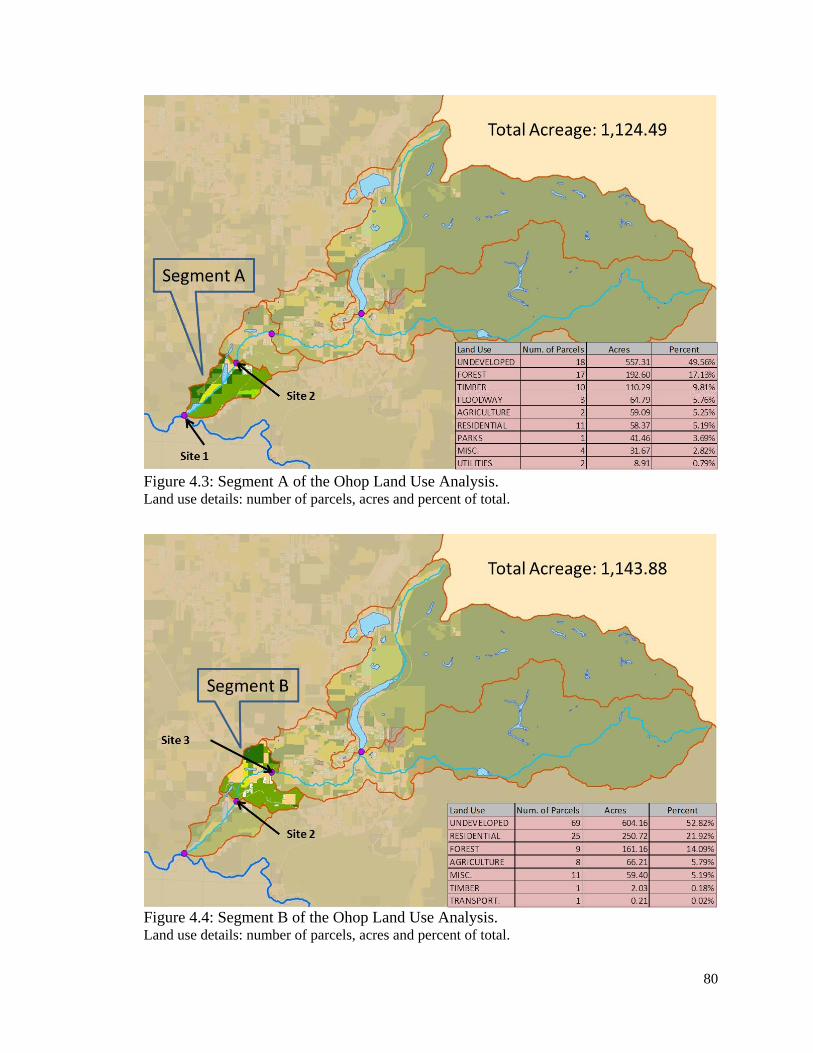
80

Figure 4.3: Segment A of the Ohop Land Use Analysis. Land use details: number of parcels, acres and percent of total.

Figure 4.4: Segment B of the Ohop Land Use Analysis. Land use details: number of parcels, acres and percent of total.

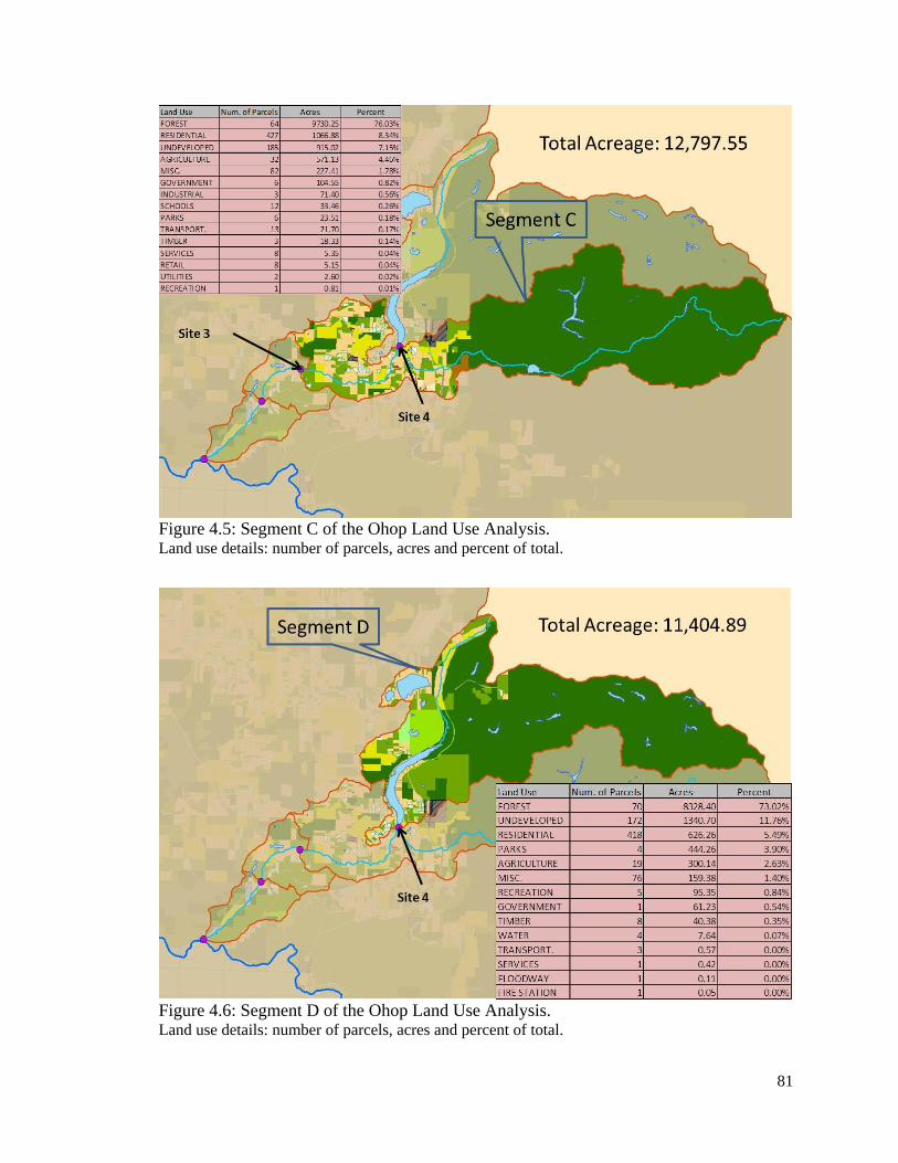
81

Figure 4.5: Segment C of the Ohop Land Use Analysis. Land use details: number of parcels, acres and percent of total.

Figure 4.6: Segment D of the Ohop Land Use Analysis. Land use details: number of parcels, acres and percent of total.

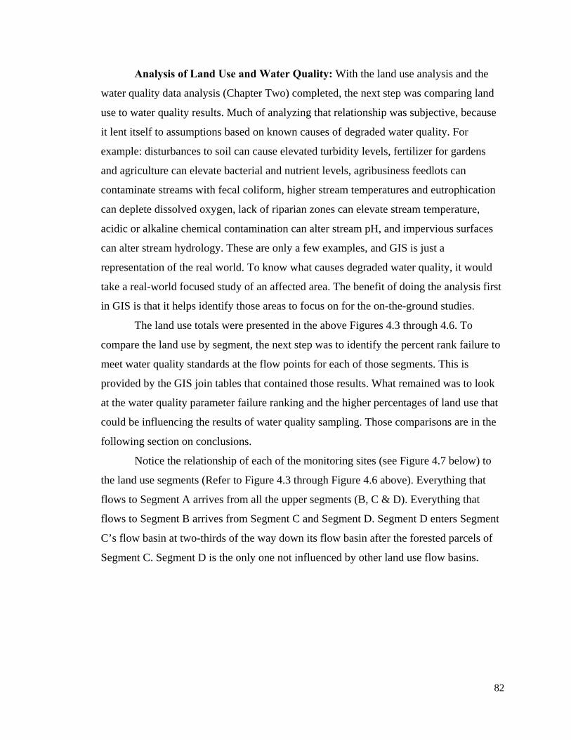
82

Analysis of Land Use and Water Quality: With the land use analysis and the

water quality data analysis (Chapter Two) completed, the next step was comparing land

use to water quality results. Much of analyzing that relationship was subjective, because

it lent itself to assumptions based on known causes of degraded water quality. For

example: disturbances to soil can cause elevated turbidity levels, fertilizer for gardens

and agriculture can elevate bacterial and nutrient levels, agribusiness feedlots can

contaminate streams with fecal coliform, higher stream temperatures and eutrophication

can deplete dissolved oxygen, lack of riparian zones can elevate stream temperature,

acidic or alkaline chemical contamination can alter stream pH, and impervious surfaces

can alter stream hydrology. These are only a few examples, and GIS is just a

representation of the real world. To know what causes degraded water quality, it would

take a real-world focused study of an affected area. The benefit of doing the analysis first

in GIS is that it helps identify those areas to focus on for the on-the-ground studies.

The land use totals were presented in the above Figures 4.3 through 4.6. To

compare the land use by segment, the next step was to identify the percent rank failure to

meet water quality standards at the flow points for each of those segments. This is

provided by the GIS join tables that contained those results. What remained was to look

at the water quality parameter failure ranking and the higher percentages of land use that

could be influencing the results of water quality sampling. Those comparisons are in the

following section on conclusions.

Notice the relationship of each of the monitoring sites (see Figure 4.7 below) to

the land use segments (Refer to Figure 4.3 through Figure 4.6 above). Everything that

flows to Segment A arrives from all the upper segments (B, C & D). Everything that

flows to Segment B arrives from Segment C and Segment D. Segment D enters Segment

C’s flow basin at two-thirds of the way down its flow basin after the forested parcels of

Segment C. Segment D is the only one not influenced by other land use flow basins.

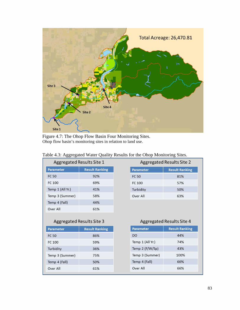
83

Figure 4.7: The Ohop Flow Basin Four Monitoring Sites. Ohop flow basin’s monitoring sites in relation to land use.

Table 4.3: Aggregated Water Quality Results for the Ohop Monitoring Sites.

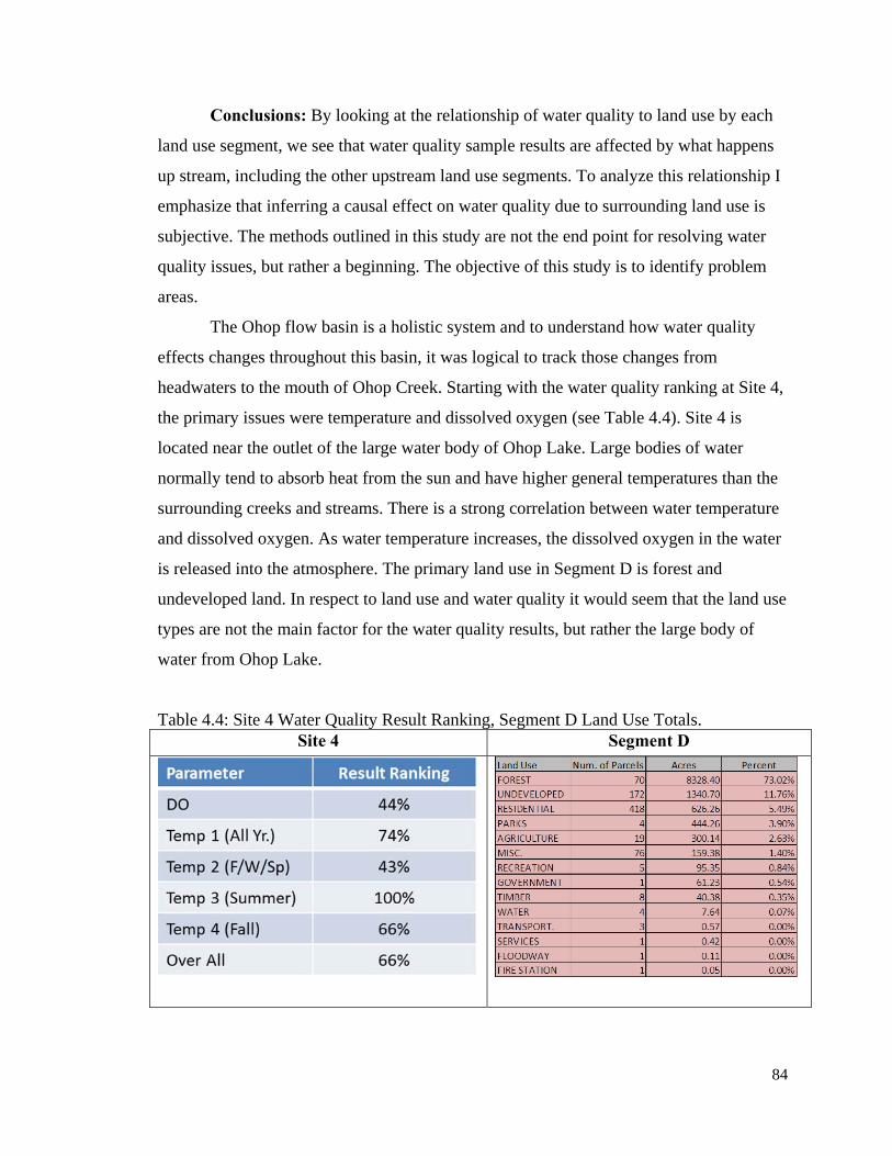
84

Conclusions: By looking at the relationship of water quality to land use by each

land use segment, we see that water quality sample results are affected by what happens

up stream, including the other upstream land use segments. To analyze this relationship I

emphasize that inferring a causal effect on water quality due to surrounding land use is

subjective. The methods outlined in this study are not the end point for resolving water

quality issues, but rather a beginning. The objective of this study is to identify problem

areas.

The Ohop flow basin is a holistic system and to understand how water quality

effects changes throughout this basin, it was logical to track those changes from

headwaters to the mouth of Ohop Creek. Starting with the water quality ranking at Site 4,

the primary issues were temperature and dissolved oxygen (see Table 4.4). Site 4 is

located near the outlet of the large water body of Ohop Lake. Large bodies of water

normally tend to absorb heat from the sun and have higher general temperatures than the

surrounding creeks and streams. There is a strong correlation between water temperature

and dissolved oxygen. As water temperature increases, the dissolved oxygen in the water

is released into the atmosphere. The primary land use in Segment D is forest and

undeveloped land. In respect to land use and water quality it would seem that the land use

types are not the main factor for the water quality results, but rather the large body of

water from Ohop Lake.

Table 4.4: Site 4 Water Quality Result Ranking, Segment D Land Use Totals. Site 4 Segment D

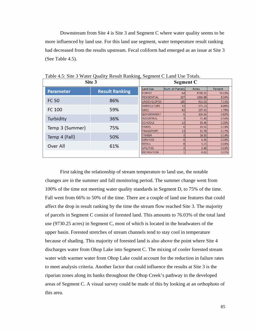
85

Downstream from Site 4 is Site 3 and Segment C where water quality seems to be

more influenced by land use. For this land use segment, water temperature result ranking

had decreased from the results upstream. Fecal coliform had emerged as an issue at Site 3

(See Table 4.5).

Table 4.5: Site 3 Water Quality Result Ranking, Segment C Land Use Totals. Site 3 Segment C

First taking the relationship of stream temperature to land use, the notable

changes are in the summer and fall monitoring period. The summer change went from

100% of the time not meeting water quality standards in Segment D, to 75% of the time.

Fall went from 66% to 50% of the time. There are a couple of land use features that could

affect the drop in result ranking by the time the stream flow reached Site 3. The majority

of parcels in Segment C consist of forested land. This amounts to 76.03% of the total land

use (9730.25 acres) in Segment C, most of which is located in the headwaters of the

upper basin. Forested stretches of stream channels tend to stay cool in temperature

because of shading. This majority of forested land is also above the point where Site 4

discharges water from Ohop Lake into Segment C. The mixing of cooler forested stream

water with warmer water from Ohop Lake could account for the reduction in failure rates

to meet analysis criteria. Another factor that could influence the results at Site 3 is the

riparian zones along its banks throughout the Ohop Creek’s pathway in the developed

areas of Segment C. A visual survey could be made of this by looking at an orthophoto of

this area.

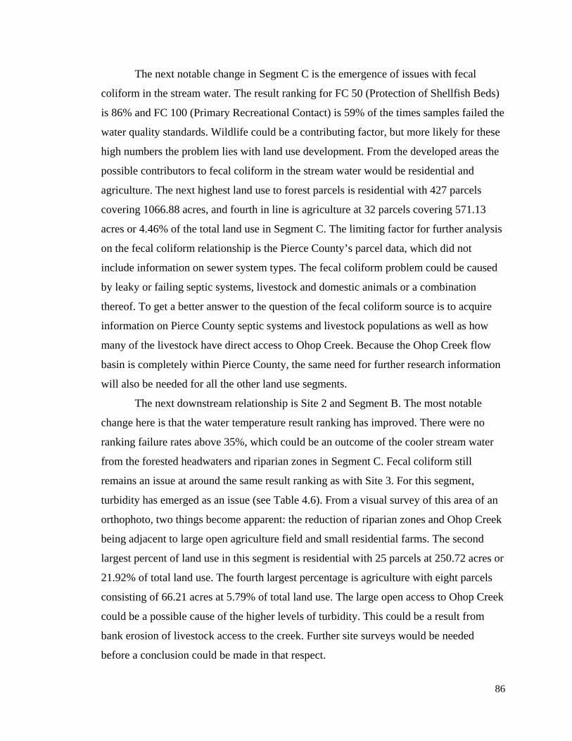
86

The next notable change in Segment C is the emergence of issues with fecal

coliform in the stream water. The result ranking for FC 50 (Protection of Shellfish Beds)

is 86% and FC 100 (Primary Recreational Contact) is 59% of the times samples failed the

water quality standards. Wildlife could be a contributing factor, but more likely for these

high numbers the problem lies with land use development. From the developed areas the

possible contributors to fecal coliform in the stream water would be residential and

agriculture. The next highest land use to forest parcels is residential with 427 parcels

covering 1066.88 acres, and fourth in line is agriculture at 32 parcels covering 571.13

acres or 4.46% of the total land use in Segment C. The limiting factor for further analysis

on the fecal coliform relationship is the Pierce County’s parcel data, which did not

include information on sewer system types. The fecal coliform problem could be caused

by leaky or failing septic systems, livestock and domestic animals or a combination

thereof. To get a better answer to the question of the fecal coliform source is to acquire

information on Pierce County septic systems and livestock populations as well as how

many of the livestock have direct access to Ohop Creek. Because the Ohop Creek flow

basin is completely within Pierce County, the same need for further research information

will also be needed for all the other land use segments.

The next downstream relationship is Site 2 and Segment B. The most notable

change here is that the water temperature result ranking has improved. There were no

ranking failure rates above 35%, which could be an outcome of the cooler stream water

from the forested headwaters and riparian zones in Segment C. Fecal coliform still

remains an issue at around the same result ranking as with Site 3. For this segment,

turbidity has emerged as an issue (see Table 4.6). From a visual survey of this area of an

orthophoto, two things become apparent: the reduction of riparian zones and Ohop Creek

being adjacent to large open agriculture field and small residential farms. The second

largest percent of land use in this segment is residential with 25 parcels at 250.72 acres or

21.92% of total land use. The fourth largest percentage is agriculture with eight parcels

consisting of 66.21 acres at 5.79% of total land use. The large open access to Ohop Creek

could be a possible cause of the higher levels of turbidity. This could be a result from

bank erosion of livestock access to the creek. Further site surveys would be needed

before a conclusion could be made in that respect.

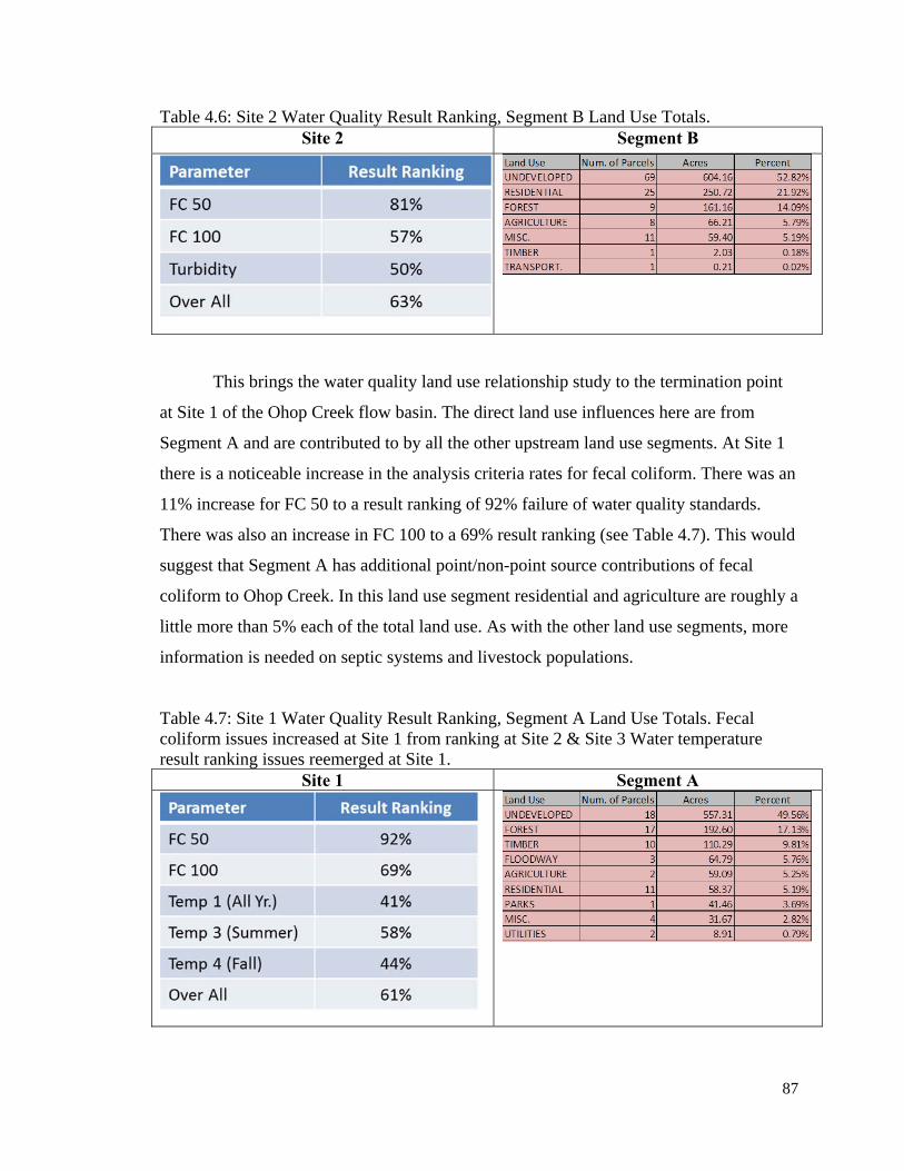
87

Table 4.6: Site 2 Water Quality Result Ranking, Segment B Land Use Totals. Site 2 Segment B

This brings the water quality land use relationship study to the termination point

at Site 1 of the Ohop Creek flow basin. The direct land use influences here are from

Segment A and are contributed to by all the other upstream land use segments. At Site 1

there is a noticeable increase in the analysis criteria rates for fecal coliform. There was an

11% increase for FC 50 to a result ranking of 92% failure of water quality standards.

There was also an increase in FC 100 to a 69% result ranking (see Table 4.7). This would

suggest that Segment A has additional point/non-point source contributions of fecal

coliform to Ohop Creek. In this land use segment residential and agriculture are roughly a

little more than 5% each of the total land use. As with the other land use segments, more

information is needed on septic systems and livestock populations.

Table 4.7: Site 1 Water Quality Result Ranking, Segment A Land Use Totals. Fecal coliform issues increased at Site 1 from ranking at Site 2 & Site 3 Water temperature result ranking issues reemerged at Site 1.

Site 1 Segment A

88

The final notable change in Segment A is that stream water temperature issues

have returned. This could be a result from the lack of riparian vegetation on both sides of

Ohop Creek. A portion of the creek runs through open fields and then is only shaded by

trees to the southeast of the channel. This allows the creek to get a good exposure of

afternoon sunlight. Riparian plantings on both sides of Ohop Creek may help to resolve

the temperature issues.

Final Thoughts:

Using water quality data analysis and developing the land use types for analyzing

the relationship between the two has been an arduous process, but well worth the effort.

This type of study can become a useful tool for the decision making process of groups

and agencies to identify those areas best suited for planning the use of restoration dollars.

The maps produced in this type of study give good geographical and tabular information

for potential project sites. The GIS information produced can be used as a platform to

receive further information as well as the creation of new spatial data as field projects

move forward.

There are two other things to acknowledge in this study about the identification of

degraded water quality in Henderson Inlet and Ohop Creek. Those two sites had already

been decided on as part of this thesis study when it was discovered those two locations

had been assigned actual restoration projects. The Department of Health and Department

of Ecology launched a Total Maximum Daily Load (TMDL) study of Henderson Inlet.

The Nisqually Indian Tribe, USFWS, South Puget Sound Salmon Enhancement Group,

National Fish and Wildlife Foundation, Stream Team and the Nisqually Land Trust did

enhancement work on the Ohop Creek channel and added plantings of riparian

vegetation. The discovery of these two major projects, midway through this thesis study,

was taken as a validation of the important work in this thesis to identify areas best suited

for environmental restoration and enhancement projects.

89

References

Allan, J. D. 1995. Stream Ecology: Structure and Function of Running Waters. The Netherlands, Kluwer Academic Publishers.

Asleson, B. C., R. S. Nestingen, J. S. Gulliver, R. M. Hozalski, & Nieber J. L. 2009.

Performance Assessment of Rain Gardens. Journal of the American Water Resources Association. Vol. 45, No. 4.

Berbells, S. 2003. 2003 Shoreline Survey of the Oakland Bay Shellfish Growing Area.

Washington State Department of Health (DOH), Public Health Advisor. Berbells, S. 2007. 2007 Shoreline Survey of the Henderson Inlet Shellfish Growing Area.

Washington State Department of Health (DOH), Health Services Consultant. Biello, D. 2011. Human Population Reaches 7 Billion – How Did This Happen and Can

It Go On? Scientific American, October 2011 Issue, Scientific American, Inc. Dethier, M. N. 2006. Native Shellfish in Nearshore Ecosystems of Puget Sound,

Technical Report 2006-04. Prepared in support of the Puget Sound Nearshore Partnership.

Dhote, S. & Dixit, S. 2009. Water Quality Improvement Through Macrophytes-A

Review. Enviromental Monitoring & Assessment; Vol. 152 Issue 1-4, p149-153. Foley, J., DeFries, R., Asner, G., Barford, C., Bonan, G., Carpenter, S., Chapin, F., Coe,

M., Daily, G., Gibbs, H., Helkowski, J., Holloway, T., Howard, E., Kucharik, C., Monfreda, C., Patz, J., Prentice, I., Ramankutty, N., Snyder, P. 2005. Global Consequence of Land Use. Science, Vol 309 July 22nd. American Association for the Advancement of Science, 1200 New Youk Ave. NW, Washington DC 20005.

Goodwin, C.L., and Pease, B. 1989. Species profiles: life histories and environmental

requirements of coastal fishes and invertebrates (Pacific Northwest)--Pacific geoduck clam. U.S. Fish. Wildlife. Serv. Biol. Rep. 82(11.120). U.S. Army Corps of Engineers, TR EL-82-4. 14 pp.

Green, J., Loft, D., and Lehr, R. 2009. State-of-the-River Report for the Chehalis River

Basin 2006-2009, A Water Quality Study. Technical Report Funded by Washington State Department of Ecology, Grays Harbor College and the Confederated Tribes of the Chehalis Reservation.

Levy, J. K., Moncur, E. T., Takara, K. 2006. Introduction: Enhancing the Capacity for

Sustainable Watershed Management. JAWRA Journal of the American Water Resources Association, Vol. 42 No. 6, pp1437-1439. USA. ISSN 1093-474X

90

Maiolo, J. R., Tschetter, P. 1981. Relating population growth to shellfish bed closures: A case study from North Carolina. Coastal Zone Management Journal, Vol. 9, Issue 1.

Mallin, M. A., Williams, K. E., Esham, E. C., Lowe, R. P. 2000. Effect of Human

Development on Bacteriological Water Quality in Coastal Watersheds. Ecological Applications by the Ecological Society of America, pp. 1047-1056

Melvin, D. J. 2006. Sanitary Survey of Nisqually Reach July 2006. Washington State

Department of Health (DOH), Office of Food Safety and Shellfish. Environmental Speciallist.

Melvin, D. 2007. Sanitary Survey of Henderson Inlet March 30, 2007. Washington State

Department of Health (DOH), Office of Shellfish and Water Protection. Nowak, D. & Walton J. 2005. Projected Urban Growth (2000-2005) and its Estimated

Impact on the US Forest Resources. Journal of Forestry 103, p383-389. Park, M-H., Suffet, I. H. & Stenstrom M. K. 2007. Utility of LANDSAT-Derived Land

Use Data for Estimating Storm-Water Pollutant Loads in an Urbanizing Area. Journal of Environmental Engineering. Vol. 133 Issue 2, p203-210.

Platt, R. H. 2006. Urban Watershed Management: Sustainability, One Stream at a Time.

Environment. Vol. 48, Issue 4. pp. 26-42 Sargeant, D., Carey, B., Roberts, M. & Brock, S. 2006 Henderson Inlet Watershed Fecal

Coliform Bacteria, Dissolved Oxygen, pH, and Temperature Total Maximum Daily Load Study. Environmental Assessment Program Washington State Department of Ecology. Olympia, Washington 98504-7710

Scholz, M. & Kazemi Yazdi S. 2009. Treatment of Road Runoff by a Combined Storm

Water Treatment, Detention and Infiltration System. Water, Air & Soil Pollution; Vol. 198 Issue 1-4, p55-64.

WA Ecology 2005. Draft: Initial Watershed Assessment Water Resource Inventory Area

13 Deschutes River Watershed. Open-File Technical Report 95-10. Prepared by: Pacific Groundwater Group, 2377 Eastlake Ave. East, Suite 200, Seattle WA 98102.

WA Ecology 2006. Water Quality Standards for Surface Water of the State of

Washington Chapter 173-201A WAC. Publication: Washington State Department of Ecology. Last update 5/6/11. Published on the web at: https://fortress.wa.gov/ecy/publications/publications/wac173201a.pdf

91

Watershed Professionals Network, llc (WPN) 2002. Nisqually River Level 1 Watershed Assessment (WRIA 11) Summary Report. Publication: Prepared for: Nisqually Watershed Planning Group

Zabel-Linclon, K. 2005. 2005 Shoreline Survey of the Nisqually Reach Shellfish Growing

Area. Washington State Department of Health (DOH), Public Health Advisor. Web Page Sources: Ecy. 2011. Puget Sound Shorelines. Department of Ecology Geological Tour of Puget

Sound. Web Site: http://www.ecy.wa.gov/programs/sea/pugetsound/tour/geology.html

Ecy-2. 2011. Deschutes River Watershed Initial Assessment, Draft May 1995.

Washington Department of Ecology Publication (Draft). Web Site: http://www.ecy.wa.gov/pubs/95158.pdf

Ecy-3. 2011. Environmental Information Management System (EIM). Washington

Department of Ecology Database Search. Web Site: http://www.ecy.wa.gov/eim/ Pierce County Public Works & Utilities, Surface Water Management (PCPWU) 2011.

Appendix C: Nisqually River Basin Risk Assessment. Flood Risk Assessment, Nisqually River Basin Plan. Partial Publication, Date Unknown. Pierce County Webpage: http://www.co.pierce.wa.us/xml/services/home/environ/water/ps/basinplans/nisqually/New082508/AppendixC-090308.pdf

US EPA (Date Unknown) Stream Channelization, Region 7 Fact Sheet Number 1. United

States Environmental Protection Agency. http://www.epa.gov/reigon7/wetlands/pdf/ChannelizedFS04-Final.pdf

WA Ecology 2006. Chapter wac173-201A WAC, Water Quality Standards for Surface

Waters of the State of Washington. (Note: Repeat) Last update 5/6/11. Published on the web at: https://fortress.wa.gov/ecy/publications/publications/wac173201a.pdf

Wahsington Department Fish and Wildlife (WDFW) 2011. Fisheries Management,

Salmonid Stock Inventory (SaSI) and State Salmon and Steelhead Stock Inventory (SASSI) reports. Web Site: http://wdfw.wa.gov/conservation/fisheries/sasi/

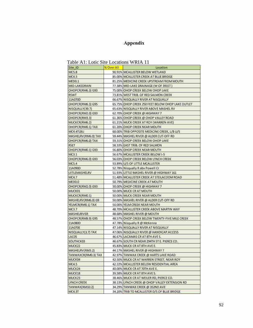
92

Appendix

Table A1: Lotic Site Locations WRIA 11 Site_ID % Over All LocationMC5.8 90.91% MCALLISTER BELOW WETLANDMC4.3 85.00% MCALLISTER CREEK AT BLUE BRIDGEMED0.1 81.25% MEDICINE CREEK UPSTREAM FROM MOUTHMID-LAKEDRAIN 77.38% MID-LAKE DRAINAGE (W OF 391ST )OHOPCR(RM6.3) G93 75.00% OHOP CREEK BELOW OHOP LAKERSWT 73.81% WEST TRIB. OF RED SALMON CREEK11A070D 66.67% NISQUALLY RIVER AT NISQUALLYOHOPCR(RM6.3) G95 65.75% OHOP CREEK 250 FEET BELOW OHOP LAKE OUTLETNISQUALLY(39.7) 65.63% NISQUALLY RIVER ABOVE MASHEL RVOHOPCR(RM2.0) G93 62.70% OHOP CREEK @ HIGHWAY 7OHOPCR(RM3.3) 61.36% OHOP CREEK @ OHOP VALLEY ROADMUCKCR(RM6.2) 61.21% MUCK CREEK AT ROY (WARREN AVE)OHOPCR(RM0.1) TAX 61.20% OHOP CREEK NEAR MOUTHMC4.4TLBU 60.00% TRIB OPPOSITE MEDICINE CREEK, L/B U/SMASHELRV(RM6.0) TAX 59.44% MASHEL RIVER @ ALDER CUT-OFF RDOHOPCR(RM6.0) TAX 59.31% OHOP CREEK BELOW OHOP LAKERSET 58.33% EAST TRIB. OF RED SALMONOHOPCR(RM0.1) G93 56.80% OHOP CREEK NEAR MOUTHMC3.1 56.67% MCALLISTER CREEK BELOW I-5OHOPCR(RM6.0) G93 56.03% OHOP CREEK BELOW LYNCH CREEKMC5.4 53.89% U/S OF LITTLE MCALLISTER11A090D 52.78% Nisqually R abv Powell CrLIITLEMASHELRV 51.93% LITTLE MASHEL RIVER @ HIGHWAY 161MC4.7 51.48% MCALLISTER CREEK AT STEILACOOM ROADMED0.0 50.79% MEDICINE CREEK AT MOUTHOHOPCR(RM2.0) G93 50.00% OHOP CREEK @ HIGHWAY 7MUCK01 50.00% MUCK CR AT MOUTHMUCKCR(RM0.1) 50.00% MUCK CREEK NEAR MOUTHMASHELRV(RM6.0) G9 50.00% MASHEL RIVER @ ALDER CUT-OFF RDYELMCR(RM0.1) TAX 50.00% YELM CREEK NEAR MOUTHMC3.7 48.70% MCALLISTER CREEK ABOVE MARTIN WAYMASHELRIVER 48.68% MASHEL RIVER @ MOUTHOHOPCR(RM9.9) G95 48.57% OHOP CREEK BELOW TWENTY-FIVE MILE CREEK11A080D 47.78% Nisqually R @ McKenna11A070E 47.14% NISQUALLY RIVER AT NISQUALLYNISQUALLY(3.7) TAX 47.06% NISQUALLY RIVER @ HANDICAP ACCESSLAC05 46.67% LACAMAS CR AT 8TH AVE S.SOUTHCK03 46.67% SOUTH CR NEAR 294TH ST E. PIERCE CO.MUCK22 45.83% MUCK CR AT 8TH AVE E.MASHELRV(RM3.2) 44.17% MASHEL RIVER @ HIGHWAY 7TANWAXCR(RM0.3) TAX 42.97% TANWAX CREEK @ HARTS LAKE ROADMUCK04 42.50% MUCK CR AT WARREN STREET, NEAR ROYMC4.5 42.22% MCALLISTER BELOW RESIDENTIAL AREAMUCK24 40.00% MUCK CR AT 70TH AVE E.MUCK18 39.58% MUCK CR AT 8TH AVE S.MUCK23 38.46% MUCK CR AT WEILER RD, PIERCE CO.LYNCH CREEK 38.13% LYNCH CREEK @ OHOP VALLEY EXTENSION RDTANWAX(RM10.2) 34.29% TANWAX CREEK @ 352ND AVEMC4.3T 34.20% TRIB TO MCALLISTER D/S OF BLUE BRIDGE

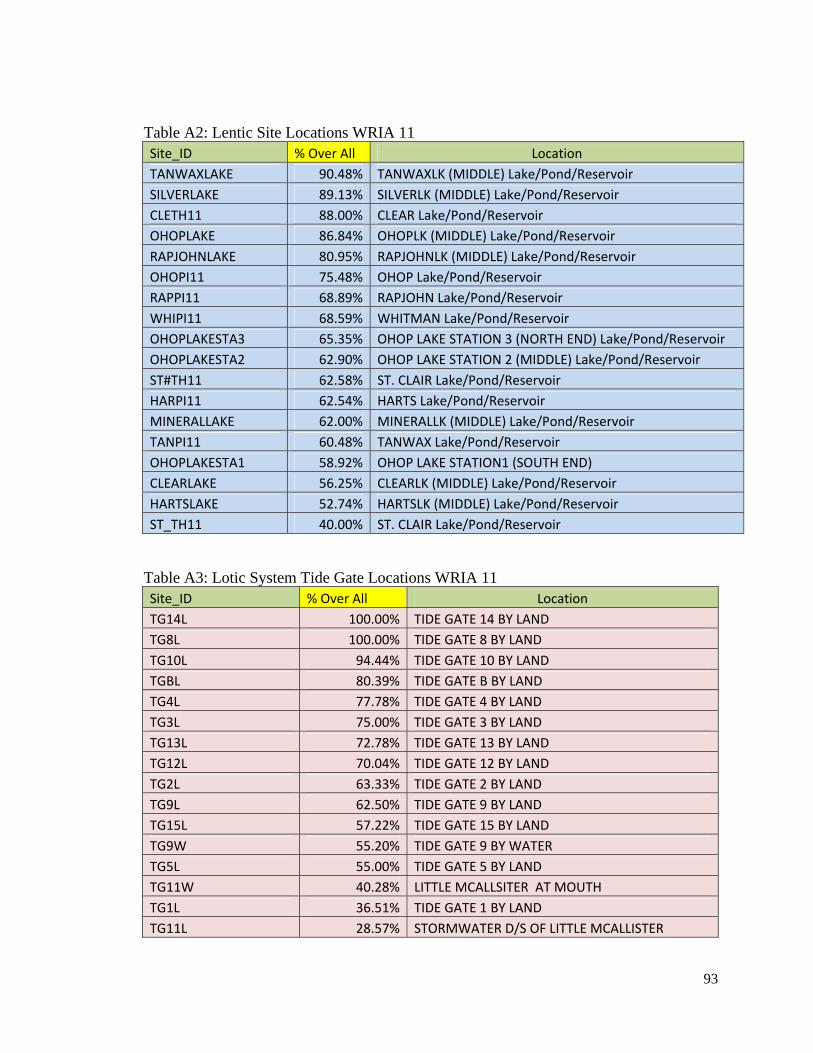
93

Table A2: Lentic Site Locations WRIA 11 Site_ID % Over All Location TANWAXLAKE 90.48% TANWAXLK (MIDDLE) Lake/Pond/Reservoir SILVERLAKE 89.13% SILVERLK (MIDDLE) Lake/Pond/Reservoir CLETH11 88.00% CLEAR Lake/Pond/Reservoir OHOPLAKE 86.84% OHOPLK (MIDDLE) Lake/Pond/Reservoir RAPJOHNLAKE 80.95% RAPJOHNLK (MIDDLE) Lake/Pond/Reservoir OHOPI11 75.48% OHOP Lake/Pond/Reservoir RAPPI11 68.89% RAPJOHN Lake/Pond/Reservoir WHIPI11 68.59% WHITMAN Lake/Pond/Reservoir OHOPLAKESTA3 65.35% OHOP LAKE STATION 3 (NORTH END) Lake/Pond/Reservoir OHOPLAKESTA2 62.90% OHOP LAKE STATION 2 (MIDDLE) Lake/Pond/Reservoir ST#TH11 62.58% ST. CLAIR Lake/Pond/Reservoir HARPI11 62.54% HARTS Lake/Pond/Reservoir MINERALLAKE 62.00% MINERALLK (MIDDLE) Lake/Pond/Reservoir TANPI11 60.48% TANWAX Lake/Pond/Reservoir OHOPLAKESTA1 58.92% OHOP LAKE STATION1 (SOUTH END) CLEARLAKE 56.25% CLEARLK (MIDDLE) Lake/Pond/Reservoir HARTSLAKE 52.74% HARTSLK (MIDDLE) Lake/Pond/Reservoir ST_TH11 40.00% ST. CLAIR Lake/Pond/Reservoir

Table A3: Lotic System Tide Gate Locations WRIA 11 Site_ID % Over All Location TG14L 100.00% TIDE GATE 14 BY LAND TG8L 100.00% TIDE GATE 8 BY LAND TG10L 94.44% TIDE GATE 10 BY LAND TGBL 80.39% TIDE GATE B BY LAND TG4L 77.78% TIDE GATE 4 BY LAND TG3L 75.00% TIDE GATE 3 BY LAND TG13L 72.78% TIDE GATE 13 BY LAND TG12L 70.04% TIDE GATE 12 BY LAND TG2L 63.33% TIDE GATE 2 BY LAND TG9L 62.50% TIDE GATE 9 BY LAND TG15L 57.22% TIDE GATE 15 BY LAND TG9W 55.20% TIDE GATE 9 BY WATER TG5L 55.00% TIDE GATE 5 BY LAND TG11W 40.28% LITTLE MCALLSITER AT MOUTH TG1L 36.51% TIDE GATE 1 BY LAND TG11L 28.57% STORMWATER D/S OF LITTLE MCALLISTER

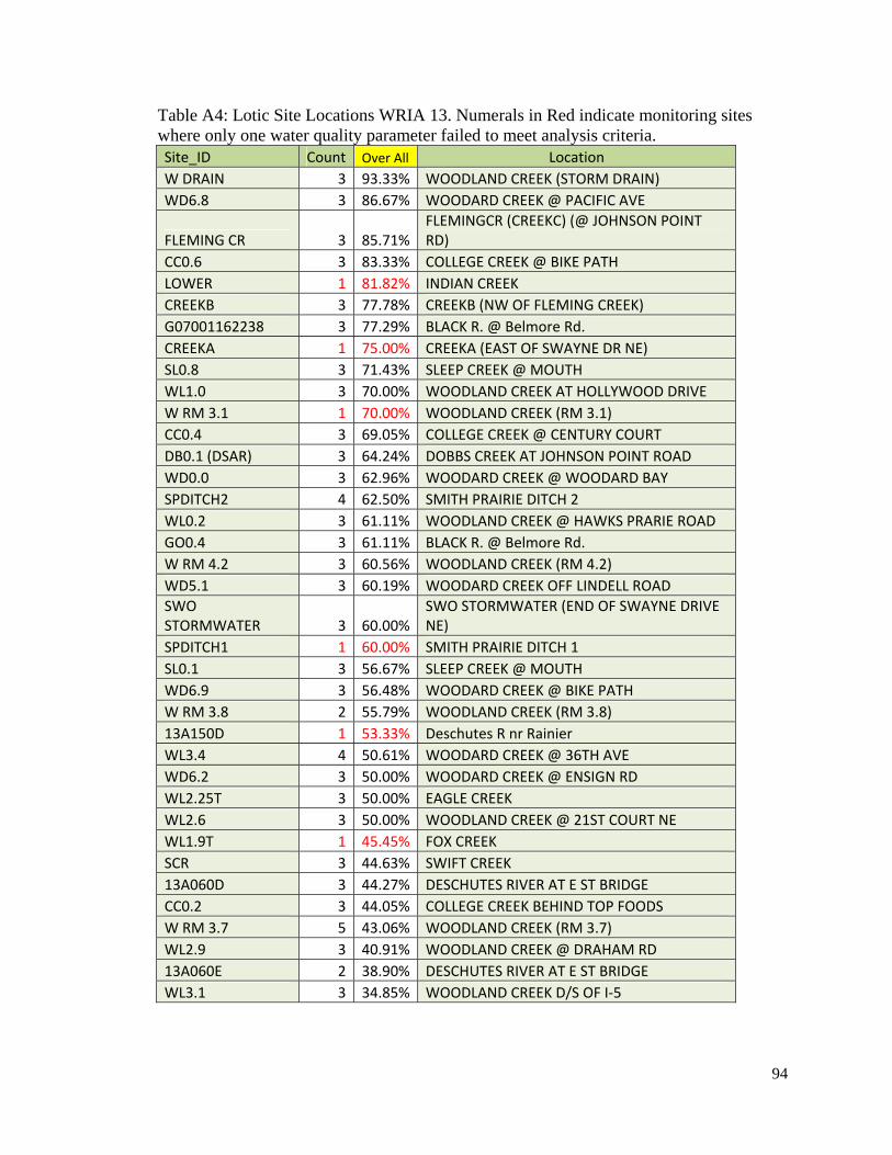
94

Table A4: Lotic Site Locations WRIA 13. Numerals in Red indicate monitoring sites where only one water quality parameter failed to meet analysis criteria. Site_ID Count Over All Location W DRAIN 3 93.33% WOODLAND CREEK (STORM DRAIN) WD6.8 3 86.67% WOODARD CREEK @ PACIFIC AVE

FLEMING CR 3 85.71%FLEMINGCR (CREEKC) (@ JOHNSON POINT RD)

CC0.6 3 83.33% COLLEGE CREEK @ BIKE PATH LOWER 1 81.82% INDIAN CREEK CREEKB 3 77.78% CREEKB (NW OF FLEMING CREEK) G07001162238 3 77.29% BLACK R. @ Belmore Rd. CREEKA 1 75.00% CREEKA (EAST OF SWAYNE DR NE) SL0.8 3 71.43% SLEEP CREEK @ MOUTH WL1.0 3 70.00% WOODLAND CREEK AT HOLLYWOOD DRIVE W RM 3.1 1 70.00% WOODLAND CREEK (RM 3.1) CC0.4 3 69.05% COLLEGE CREEK @ CENTURY COURT DB0.1 (DSAR) 3 64.24% DOBBS CREEK AT JOHNSON POINT ROAD WD0.0 3 62.96% WOODARD CREEK @ WOODARD BAY SPDITCH2 4 62.50% SMITH PRAIRIE DITCH 2 WL0.2 3 61.11% WOODLAND CREEK @ HAWKS PRARIE ROAD GO0.4 3 61.11% BLACK R. @ Belmore Rd. W RM 4.2 3 60.56% WOODLAND CREEK (RM 4.2) WD5.1 3 60.19% WOODARD CREEK OFF LINDELL ROAD SWO STORMWATER 3 60.00%

SWO STORMWATER (END OF SWAYNE DRIVE NE)

SPDITCH1 1 60.00% SMITH PRAIRIE DITCH 1 SL0.1 3 56.67% SLEEP CREEK @ MOUTH WD6.9 3 56.48% WOODARD CREEK @ BIKE PATH W RM 3.8 2 55.79% WOODLAND CREEK (RM 3.8) 13A150D 1 53.33% Deschutes R nr Rainier WL3.4 4 50.61% WOODARD CREEK @ 36TH AVE WD6.2 3 50.00% WOODARD CREEK @ ENSIGN RD WL2.25T 3 50.00% EAGLE CREEK WL2.6 3 50.00% WOODLAND CREEK @ 21ST COURT NE WL1.9T 1 45.45% FOX CREEK SCR 3 44.63% SWIFT CREEK 13A060D 3 44.27% DESCHUTES RIVER AT E ST BRIDGE CC0.2 3 44.05% COLLEGE CREEK BEHIND TOP FOODS W RM 3.7 5 43.06% WOODLAND CREEK (RM 3.7) WL2.9 3 40.91% WOODLAND CREEK @ DRAHAM RD 13A060E 2 38.90% DESCHUTES RIVER AT E ST BRIDGE WL3.1 3 34.85% WOODLAND CREEK D/S OF I-5

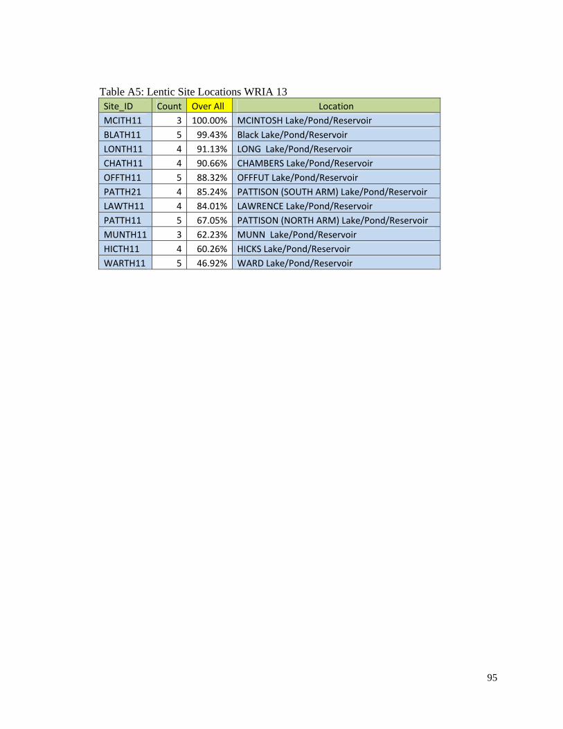
95

Table A5: Lentic Site Locations WRIA 13 Site_ID Count Over All Location MCITH11 3 100.00% MCINTOSH Lake/Pond/Reservoir BLATH11 5 99.43% Black Lake/Pond/Reservoir LONTH11 4 91.13% LONG Lake/Pond/Reservoir CHATH11 4 90.66% CHAMBERS Lake/Pond/Reservoir OFFTH11 5 88.32% OFFFUT Lake/Pond/Reservoir PATTH21 4 85.24% PATTISON (SOUTH ARM) Lake/Pond/Reservoir LAWTH11 4 84.01% LAWRENCE Lake/Pond/Reservoir PATTH11 5 67.05% PATTISON (NORTH ARM) Lake/Pond/Reservoir MUNTH11 3 62.23% MUNN Lake/Pond/Reservoir HICTH11 4 60.26% HICKS Lake/Pond/Reservoir WARTH11 5 46.92% WARD Lake/Pond/Reservoir

Documents

IDENTIFICATION OF DEGRADED LOTIC FRESHWATER THAT AFFECTS