Embed Size (px)
Citation preview
1
Identification of Potential Reservoir sands within the Torok Formation
in a northern portion of the National Petroleum Reserve – Alaska
By: Javier Herbas
Department of Earth and Planetary Science McGill University
Montreal, Quebec, Canada
Submitted: October 02, 2009
A thesis submitted to McGill University in partial fulfillment of the requirements of the degree of Master of Science
@ J. Herbas 2009
2
ABSTRACT
This thesis examines the seismic responses of potential hydrocarbon
charged sandstone reservoirs within the Torok xxxFormation in a northern
portion of the National Petroleum Reserve – Alaska (NPRA). By integrating
wireline logs, 3D seismic data, seismic attributes and modeling, I show that
the most prospective sandstones are those characterized by a decrease in
their p-wave, an increase in their s-wave, a suggested increase in porosity
(by the density wireline log), and a decrease in Poisson‟s ratio which
causes AVO anomalies Class II and III.
Similar to other sandstones deposited in turbidite channels in the NPRA,
some of these potentially porous Lower Torok sandstones show an
increase in their absolute amplitude values with an increasing offset
(negative gradient) and a negative or positive intercept. This work suggests
that those amplitude anomalous responses could be due to the presence of
fluid saturated sandstones, which cause the decrease and corresponding
increase in p and s-waves that result in a low Poisson‟s ratio and in the
definition of the Class II and III AVO anomalies.
3
RESUME
Cette thèse étudie la réponse sismique de réservoirs potentiels chargés
d‟hydrocarbure, formés de grès appartenant à la formation Torok et situés
dans la partie nord de la réserve nationale d‟hydrocarbure de l‟Alaska
(NPRA). En intégrant les diagraphies, les données sismiques 3D, les
attributs sismiques et la modélisation, je démontrons que les grès les plus
prospectifs sont caractérisés par une diminution de leur amplitude d‟onde
de compression, une augmentation de leur amplitude d‟onde transversale,
une augmentation suggérée de la porosité (diagraphie de densité) et une
diminution du coefficient de Poisson qui cause des anomalies AVO
(variation de l‟amplitude avec le déport) de classe II et III.
Comme pour d‟autres grès déposés dans des chenaux de turbidite dans la
région du NPRA, certains de ces grès potentiellement poreux de la
formation Lower Torok démontrent une augmentation de leur valeur
absolue d‟amplitude avec un déport augmentant (gradient négatif) et une
valeur positive ou négative pour un déport de zéro. Ce travail suggère que
ces réponses d‟amplitudes anormales pourraient être causées par la
présence de grès saturés en fluide, ce qui cause une diminution de
l‟amplitude des ondes de compression et une augmentation
correspondante de l‟amplitude des ondes transversales, ce qui résulte en
un coefficient de Poisson moins élevé et en une définition des anomalies
AVO de classe II et III.
4
THESIS FORMAT
This thesis was done based on a paper format and it consists of three
chapters: Chapter I introduces the geological background of the area, data
available, methodology applied and objectives of this case study; chapter II,
which is the paper itself; and chapter III that refers to the study conclusions.
Additionally, this report has 6 appendices that go through all the
mathematical and geophysical background to support the methodology and
workflows applied. All pages within this thesis were formatted to meet the
guidelines from the thesis preparation document prepared by the faculty of
Graduate Studies and Research from McGill University.
CONTRIBUTION OF AUTHORS
I hereby declare that all practical and analytical aspects of the research
described herein has been performed and carried out by myself, Javier
Herbas. Guidance and supervision was given by Wayne Park, Dr. Andrew
Willis and Dr. Bruce Hart to ensure a rigorous scientific method was upheld
and adhered to throughout the work.

5
ACKNOWLEDGEMENTS
I will like to give special thanks to my family, Julio Herbas (father), Nelida de
Herbas (mother), Andreina Herbas (sister) and Aaron Mendez (brother in
law) for all the support and strength they gave me throughout the course of
my Master Program, and to my girlfriend Michaela Bjorseth for helping me
by being supportive and being very patient while I was writing this thesis.
Without all you guys I could not have finished my MSc.
I wish to thank Petro-Canada, who cordially sponsored the thesis project
over its duration and contributed with great technical and intellectual
discussions via my mentors, namely Wayne Park and Andrew Willis;
WesternGeco for providing the 3-D seismic survey and allowing me to
publish the result of this study. Special thanks to Jeff Bever (Alaska Team
Leader) and Derek Evoy (Alaska Regional Manager) for giving me the
opportunity to work in their team while doing my MSc thesis; to Todor
Todorov for his assistance with the AVO Modeling, Anne Halladay for all the
attribute analysis discussions; to my very good friend Cindy Koo for going
over my thesis several times and for the great times in the mountains; to
Tim McCullagh for allowing me to use his thesis as a guide, to Charles
Boyer and Jonathan Menivier for helping me with the abstract translation
from English to French, and to Dr. Bruce Hart for all his guidance,
suggestions and thesis corrections.
6
TABLE OF CONTENTS
Abstract……………………………………………………………………………2
Resume……………………………………………………………………………3
Thesis format……………………………………………………………………...4
Contribution of authors………………………………………………………......4
Acknowledgements……………………………………………………………....5
List of Figures………………………………………………………………….....8
List of Tables…………………………………………………………………….19
List of appendices……………………………………………………………….19
Chapter one – Introduction to study…………………………………………...20
Introduction………………………………………………………………...20
NPRA history……………………………………………………….…......22
Previous work……………………………………………………………..23
Objectives……………………………………………………….…………24
Database and Methods……………………………………….………….25
Chapter two – Identification of potential reservoir sands within the Torok
Formation in a northern portion of the National Petroleum Reserves –
Alaska………………………………………………………………………….....27
Abstract…………………………………………………………………….27
Introduction………………………………………………………………...27
Geological Setting………………………………………………………...29
Stratigraphic and structure of the Brookian turbidite play…………….30
Source rocks………………………………………………………………31
Study area, database and methods…………………………………….33
Results……………………………………………………………………..35

7
1. Seismic calibration and mapping…………………………….35
2. AVO modeling………………………………………………….38
3. Seismic attributes………………………………….…………..41
Discussion………..…………………………………………….……..…...45
1. Depositional geomorphology…………………………………45
2. Amplitude anomalies……………………………….…………46
3. Seismic attribute analysis………………………….…………49
Conclusions……………………………………………………….……….50
Acknowledgments………………………………………………….……..52
Chapter three – Conclusions of study…………………………………..........98
References…………………………………………………………….....101
Appendices……………………………………………………………………..109
8
LIST OF FIGURES
Figure 1: Base map displaying major geologic provinces within the NPRA
(boundary indicated by cyan line), namely, the Barrow arch, the Colville
foreland basin, the foothills fold belt, and the Brooks Range overthrust.
These provinces overlap to varying degrees, but can be divided on the
basis of geological history affecting known and possible petroleum
occurrence (Montgomery, 1998). Some of the known oil and gas
accumulations are displayed on the map on green and red, respectively.
The seismic survey used is within the northern part of the NPRA. Its exact
location cannot be revealed due to confidentiality agreements. Additionally,
the map includes the location of the Tarn and Meltwater fields, which are
two of the most recent discoveries made on bottom-sets on the North Slope
of Alaska, plus the Kuparuk River Field, which is the second largest in North
America following Prudeau Bay………………….………………..…………..53
Figure 2. Seismic expression of Brookian depositional style in the eastern
part of the NPRA showing topset, clinoform, and bottomset strata
geometries and relation to the LCU and Beaufortian sequence. Location of
this 2D seismic section is displayed with a red line on base map (left). A
secondary green transect is displayed on the base map which represents
the west-to-east orientation of the seismic section from Figure 4……..…54
Figure 3. Chronostratigraphic column for the Colville foreland basin,
northern Alaska, showing revised stratigraphic nomenclature and ages of
units (Mull et al, 2003)…………………………………………………………..55
Figure 4 .West-to-east transect built out of 2D lines extracted from the
USGS (Unite States Geological Survey) data base. Two strong reflectors
were interpreted; the LCU (upper in red), and the Shublik (lower in green),
plus the major faults towards the east. Above the LCU lies the HRZ (one of
the well known source rocks in the NPRA), which has on top prograding
9
clinoforms towards the east that represent the basin filling pattern. Location
of this transect is displayed on top of a base map on Figure 2 with green..56
Figure 5. Seismic section with a west-to-east orientation with 4 different
seismic files: a) full stack time-migrated seismic data processed with a non
AVO friendly sequence, b) full stack time-migrated seismic data processed
with an AVO friendly sequence, c) near angle stack seismic data generated
by stacking shot gathers from 10 to 20 degrees, and d) far angle stack
seismic data generated by stacking shot gathers from 30 to 40 degrees. All
the sections have well A overlain, which has a GR log (purple) displayed on
its left, a sonic log on its right (green), and a synthetic seismogram in the
middle (green). Amplitude increases between the near (c) and the far (d)
angle stacks are very prominent and easy to visualize, in particular on some
of the troughs closer to the left of the section. The full stack time-migrated
seismic file (a) was used for horizon picking since the events are more
continuous, although for seismic attribute extraction purposes, the AVO
friendly was the one used because the compliant processing sequence
applied preserves the amplitudes. ..…………………………………….........58
Figure 6. Well A displaying zero-offset synthetic seismograms generated
with three different types of wavelets (Butterworth, Ormsby and Ricker).
Best result was achieved with the 10, 18, 50, 72 Hz Butterworth with no
phase rotation. Two strong markers (HRZ and LCU) used for calibration are
displayed at the bottom. GR logs are displayed on the left (purple curves)
and DT logs to the right (green curves). High slope channels (shallower)
and the basin floor fans (deeper – above the HRZ marker) are displayed on
the GR log. Synthetics seismograms have not been stretched nor
compressed in order to try and preserve velocities as much as possible.
Yellow rectangles show the correlation window used, with the best values
achieved at the bottom below the HRZ and LCU markers, whereas above
these, the ties were rather poor, possibly due to the event thicknesses
(below seismic resolution), lateral lithology variations, and/or the type of
10
migration (time migration) and algorithm used. See Figure 6 for exploded
synthetic and further analysis………………………………………..........…..60
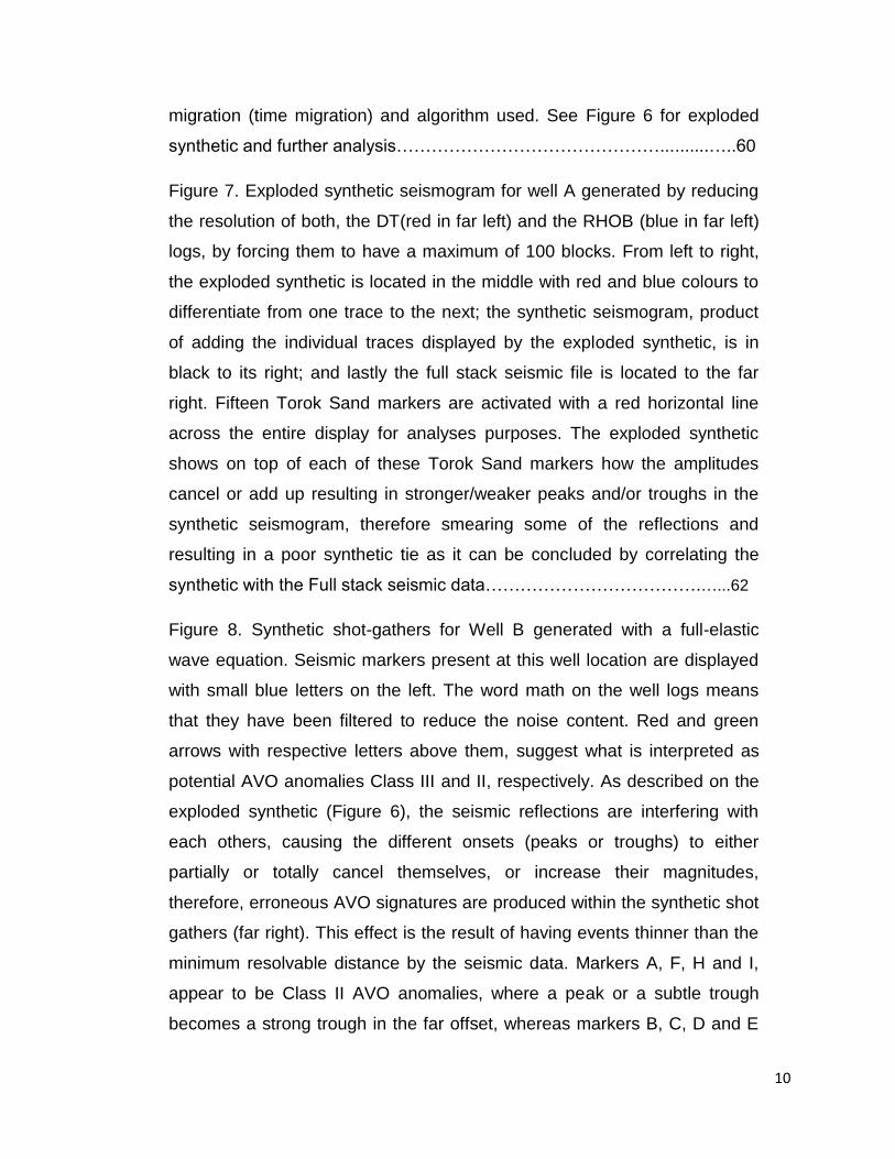
Figure 7. Exploded synthetic seismogram for well A generated by reducing
the resolution of both, the DT(red in far left) and the RHOB (blue in far left)
logs, by forcing them to have a maximum of 100 blocks. From left to right,
the exploded synthetic is located in the middle with red and blue colours to
differentiate from one trace to the next; the synthetic seismogram, product
of adding the individual traces displayed by the exploded synthetic, is in
black to its right; and lastly the full stack seismic file is located to the far
right. Fifteen Torok Sand markers are activated with a red horizontal line
across the entire display for analyses purposes. The exploded synthetic
shows on top of each of these Torok Sand markers how the amplitudes
cancel or add up resulting in stronger/weaker peaks and/or troughs in the
synthetic seismogram, therefore smearing some of the reflections and
resulting in a poor synthetic tie as it can be concluded by correlating the
synthetic with the Full stack seismic data……………………………….…...62
Figure 8. Synthetic shot-gathers for Well B generated with a full-elastic
wave equation. Seismic markers present at this well location are displayed
with small blue letters on the left. The word math on the well logs means
that they have been filtered to reduce the noise content. Red and green
arrows with respective letters above them, suggest what is interpreted as
potential AVO anomalies Class III and II, respectively. As described on the
exploded synthetic (Figure 6), the seismic reflections are interfering with
each others, causing the different onsets (peaks or troughs) to either
partially or totally cancel themselves, or increase their magnitudes,
therefore, erroneous AVO signatures are produced within the synthetic shot
gathers (far right). This effect is the result of having events thinner than the
minimum resolvable distance by the seismic data. Markers A, F, H and I,
appear to be Class II AVO anomalies, where a peak or a subtle trough
becomes a strong trough in the far offset, whereas markers B, C, D and E
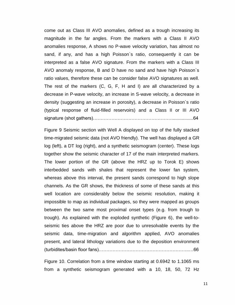
11
come out as Class III AVO anomalies, defined as a trough increasing its
magnitude in the far angles. From the markers with a Class II AVO
anomalies response, A shows no P-wave velocity variation, has almost no
sand, if any, and has a high Poisson`s ratio, consequently it can be
interpreted as a false AVO signature. From the markers with a Class III
AVO anomaly response, B and D have no sand and have high Poisson`s
ratio values, therefore these can be consider false AVO signatures as well.
The rest of the markers (C, G, F, H and I) are all characterized by a
decrease in P-wave velocity, an increase in S-wave velocity, a decrease in
density (suggesting an increase in porosity), a decrease in Poisson`s ratio
(typical response of fluid-filled reservoirs) and a Class II or III AVO
signature (shot gathers)…………………………………………….................64
Figure 9 Seismic section with Well A displayed on top of the fully stacked
time-migrated seismic data (not AVO friendly). The well has displayed a GR
log (left), a DT log (right), and a synthetic seismogram (center). These logs
together show the seismic character of 17 of the main interpreted markers.
The lower portion of the GR (above the HRZ up to Torok E) shows
interbedded sands with shales that represent the lower fan system,
whereas above this interval, the present sands correspond to high slope
channels. As the GR shows, the thickness of some of these sands at this
well location are considerably below the seismic resolution, making it
impossible to map as individual packages, so they were mapped as groups
between the two same most proximal onset types (e.g. from trough to
trough). As explained with the exploded synthetic (Figure 6), the well-to-
seismic ties above the HRZ are poor due to unresolvable events by the
seismic data, time-migration and algorithm applied, AVO anomalies
present, and lateral lithology variations due to the deposition environment
(turbidites/basin floor fans)…………………………………………………..…66
Figure 10. Correlation from a time window starting at 0.6942 to 1.1065 ms
from a synthetic seismogram generated with a 10, 18, 50, 72 Hz
12
Butterworth wavelet from Well A. The polarity used was normal and the
maximum correlation coefficient achieved was 0.673. The correlation
coefficients suggested that a bulk time shift of 208 ms was needed plus a
relative phase rotation of 6 degree, which was not corrected due to its
numerical size. This synthetic was generated from the southernmost well,
where the clinoforms tend to thin down. The low correlation could be due in
part to the thickness of the high slope channels and the interbedded sands
with shales being below tunning (below seismic resolution), lateral lithology
variations caused by the presence of many channels, low signal to noise
ratio, and/or the presence of the AVO anomalies above the HRZ marker..68
Figure 11. Time structural maps of markers HRZ, E, I, J, K, and L. Hot
colours (towards yellow) indicate shallow values whereas colder (towards
blue) are indicating deeper intervals. These time structural maps suggest
that the highs are located to the west with a northeastern to southwestern
orientation that dips towards the east, which follows the basin filling pattern
of the North Slope of Alaska (Figure 13). The HRZ map suggests the
presence of a subtle high or anticline (black arrow in map a) that thins as it
passes down the slope to the south east, whereas as it gets shallower,
markers I, J, and K suggest an additional pattern towards the south, where
there is a pronounced low (black arrow on maps c, d and e) that appears to
get partially filled up as marker L is reached (map f)…...……………….…..70
Figure 12. Composite of isochrons where the base of each map
corresponds to the HRZ, the top or shallower markers are surfaces that get
younger in age starting with marker G (a) all the way to marker L (f). Color
bars used are the same for the six maps, with red to yellow displaying
shallow values, and dark blue representing deeper contours. This set of
maps clearly show the west-to-east depositional filling pattern reflected by
contours with an approximate south-to-north trend and an east dip that
indicates the filling pattern over the slope towards the basin as the seismic
transect from Figure 4 also suggests. Isochrons for intervals H, I, J, K, and
13
L suggest the presence of a low (black arrow in each map), easily
recognized with the white trend line between the yellow and light blue
colors. This low could potentially be a good location for sediment deposits
that were carried by currents down the slope………………………………..72
Figure 13. Composite isochrons for individual intervals with constant color
bar, where hot colors (towards red) represent thicker intervals and cold
colors (towards dark blue) thin intervals. These isochrons together suggest
that the depocenter of the bodies (red–to-yellow) deposited on top of the
slope migrated with a north-eastern-to-south-western trend, giving this way
an idea of how the sediments got deposited by always looking for the lower
part on the relief of the slope that corresponded to the previous lobes. This
is the expected behavior as currents always look for the deeper or lower
paths to go through and thus deposit part of their sediment loads on their
paths. a) interval D-E with two dashed arrows that show the trends of the
thickest parts of the isochron where it was assume that the biggest
sediment load was deposited; b) interval E-Ea with one dashed arrow that
follows the thickest part of this body which appear to be accommodated
approximately between the two previous depocenters from D-E; c) interval
Ea-F, again with two dashed arrows, one that migrated to the south,
whereas the other (northern one) seems to have filled in the thinner part
(blue) from interval E-Ea; d) interval F-G showing scattered bodies that are
the response of probably thin sands or interbedded sands with shales
below the seismic resolution; e) interval J-K with two dashed arrows to the
south on top of what could be one or two depocenters; and f) interval K-L
with two dashed arrow following two potential depocenters that partially
filled what seemed to be thinner intervals from J-K….....……….…………..79
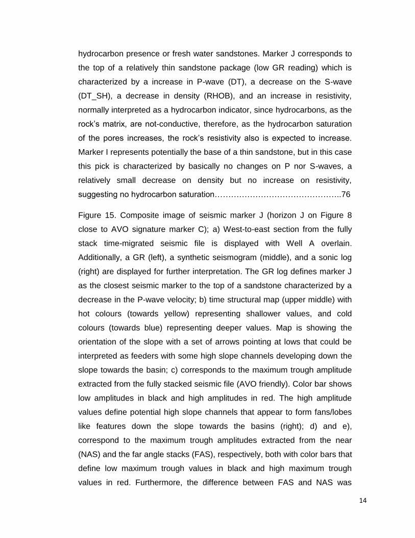
Figure 14. Wireline logs corresponding to Well A with seismic markers J
(green), I (red) and HRZ (blue) displayed. Two cut-off values were applied;
a first one of 120 to indicate sandstones (yellow) on the GR, and a second
of 10 ohm.m on the resistivity logs (red vertical line) to indicate potential
14
hydrocarbon presence or fresh water sandstones. Marker J corresponds to
the top of a relatively thin sandstone package (low GR reading) which is
characterized by a increase in P-wave (DT), a decrease on the S-wave
(DT_SH), a decrease in density (RHOB), and an increase in resistivity,
normally interpreted as a hydrocarbon indicator, since hydrocarbons, as the
rock‟s matrix, are not-conductive, therefore, as the hydrocarbon saturation
of the pores increases, the rock‟s resistivity also is expected to increase.
Marker I represents potentially the base of a thin sandstone, but in this case
this pick is characterized by basically no changes on P nor S-waves, a
relatively small decrease on density but no increase on resistivity,
suggesting no hydrocarbon saturation………………………………………..76
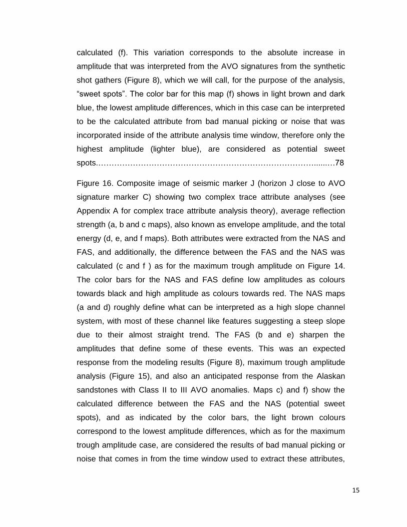
Figure 15. Composite image of seismic marker J (horizon J on Figure 8
close to AVO signature marker C); a) West-to-east section from the fully
stack time-migrated seismic file is displayed with Well A overlain.
Additionally, a GR (left), a synthetic seismogram (middle), and a sonic log
(right) are displayed for further interpretation. The GR log defines marker J
as the closest seismic marker to the top of a sandstone characterized by a
decrease in the P-wave velocity; b) time structural map (upper middle) with
hot colours (towards yellow) representing shallower values, and cold
colours (towards blue) representing deeper values. Map is showing the
orientation of the slope with a set of arrows pointing at lows that could be
interpreted as feeders with some high slope channels developing down the
slope towards the basin; c) corresponds to the maximum trough amplitude
extracted from the fully stacked seismic file (AVO friendly). Color bar shows
low amplitudes in black and high amplitudes in red. The high amplitude
values define potential high slope channels that appear to form fans/lobes
like features down the slope towards the basins (right); d) and e),
correspond to the maximum trough amplitudes extracted from the near
(NAS) and the far angle stacks (FAS), respectively, both with color bars that
define low maximum trough values in black and high maximum trough
values in red. Furthermore, the difference between FAS and NAS was
15
calculated (f). This variation corresponds to the absolute increase in
amplitude that was interpreted from the AVO signatures from the synthetic
shot gathers (Figure 8), which we will call, for the purpose of the analysis,
“sweet spots”. The color bar for this map (f) shows in light brown and dark
blue, the lowest amplitude differences, which in this case can be interpreted
to be the calculated attribute from bad manual picking or noise that was
incorporated inside of the attribute analysis time window, therefore only the
highest amplitude (lighter blue), are considered as potential sweet
spots.………………………………………………………………………......…78
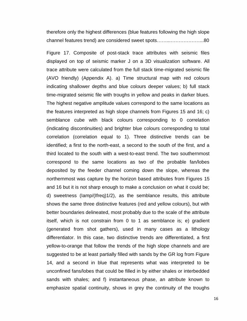
Figure 16. Composite image of seismic marker J (horizon J close to AVO
signature marker C) showing two complex trace attribute analyses (see
Appendix A for complex trace attribute analysis theory), average reflection
strength (a, b and c maps), also known as envelope amplitude, and the total
energy (d, e, and f maps). Both attributes were extracted from the NAS and
FAS, and additionally, the difference between the FAS and the NAS was
calculated (c and f ) as for the maximum trough amplitude on Figure 14.
The color bars for the NAS and FAS define low amplitudes as colours
towards black and high amplitude as colours towards red. The NAS maps
(a and d) roughly define what can be interpreted as a high slope channel
system, with most of these channel like features suggesting a steep slope
due to their almost straight trend. The FAS (b and e) sharpen the
amplitudes that define some of these events. This was an expected
response from the modeling results (Figure 8), maximum trough amplitude
analysis (Figure 15), and also an anticipated response from the Alaskan
sandstones with Class II to III AVO anomalies. Maps c) and f) show the
calculated difference between the FAS and the NAS (potential sweet
spots), and as indicated by the color bars, the light brown colours
correspond to the lowest amplitude differences, which as for the maximum
trough amplitude case, are considered the results of bad manual picking or
noise that comes in from the time window used to extract these attributes,
16
therefore only the highest differences (blue features following the high slope
channel features trend) are considered sweet spots……...………………...80
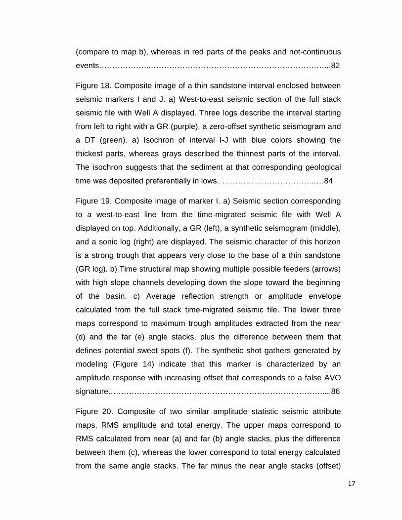
Figure 17. Composite of post-stack trace attributes with seismic files
displayed on top of seismic marker J on a 3D visualization software. All
trace attribute were calculated from the full stack time-migrated seismic file
(AVO friendly) (Appendix A). a) Time structural map with red colours
indicating shallower depths and blue colours deeper values; b) full stack
time-migrated seismic file with troughs in yellow and peaks in darker blues.
The highest negative amplitude values correspond to the same locations as
the features interpreted as high slope channels from Figures 15 and 16; c)
semblance cube with black colours corresponding to 0 correlation
(indicating discontinuities) and brighter blue colours corresponding to total
correlation (correlation equal to 1). Three distinctive trends can be
identified; a first to the north-east, a second to the south of the first, and a
third located to the south with a west-to-east trend. The two southernmost
correspond to the same locations as two of the probable fan/lobes
deposited by the feeder channel coming down the slope, whereas the
northernmost was capture by the horizon based attributes from Figures 15
and 16 but it is not sharp enough to make a conclusion on what it could be;
d) sweetness (Iamp/(Ifreq)1/2), as the semblance results, this attribute
shows the same three distinctive features (red and yellow colours), but with
better boundaries delineated, most probably due to the scale of the attribute
itself, which is not constrain from 0 to 1 as semblance is; e) gradient
(generated from shot gathers), used in many cases as a lithology
differentiator. In this case, two distinctive trends are differentiated, a first
yellow-to-orange that follow the trends of the high slope channels and are
suggested to be at least partially filled with sands by the GR log from Figure
14, and a second in blue that represents what was interpreted to be
unconfined fans/lobes that could be filled in by either shales or interbedded
sands with shales; and f) instantaneous phase, an attribute known to
emphasize spatial continuity, shows in grey the continuity of the troughs
17
(compare to map b), whereas in red parts of the peaks and not-continuous
events………………..…………………………………………………………...82
Figure 18. Composite image of a thin sandstone interval enclosed between
seismic markers I and J. a) West-to-east seismic section of the full stack
seismic file with Well A displayed. Three logs describe the interval starting
from left to right with a GR (purple), a zero-offset synthetic seismogram and
a DT (green). a) Isochron of interval I-J with blue colors showing the
thickest parts, whereas grays described the thinnest parts of the interval.
The isochron suggests that the sediment at that corresponding geological
time was deposited preferentially in lows………………………………..…84
Figure 19. Composite image of marker I. a) Seismic section corresponding
to a west-to-east line from the time-migrated seismic file with Well A
displayed on top. Additionally, a GR (left), a synthetic seismogram (middle),
and a sonic log (right) are displayed. The seismic character of this horizon
is a strong trough that appears very close to the base of a thin sandstone
(GR log). b) Time structural map showing multiple possible feeders (arrows)
with high slope channels developing down the slope toward the beginning
of the basin. c) Average reflection strength or amplitude envelope
calculated from the full stack time-migrated seismic file. The lower three
maps correspond to maximum trough amplitudes extracted from the near
(d) and the far (e) angle stacks, plus the difference between them that
defines potential sweet spots (f). The synthetic shot gathers generated by
modeling (Figure 14) indicate that this marker is characterized by an
amplitude response with increasing offset that corresponds to a false AVO
signature.……………………………..……………………………………….....86
Figure 20. Composite of two similar amplitude statistic seismic attribute
maps, RMS amplitude and total energy. The upper maps correspond to
RMS calculated from near (a) and far (b) angle stacks, plus the difference
between them (c), whereas the lower correspond to total energy calculated
from the same angle stacks. The far minus the near angle stacks (offset)
18
define the difference in amplitude with increasing offset, which according to
the synthetic shot gathers correspond to amplitude responses that
correspond to seismic background. Color bars for the total energy (d, e, and
f) outputs where adjusted in order to sharpen the false AVO signatures
described in the far angles……………………………....……………………..88
Figure 21. Summary of RMS amplitudes of randomly selected markers
within the Torok Formation calculated from far angle stacks (FAS) to isolate
the amplitude responses with increasing offset. By isolating these
responses from the FAS, amplitude responses with increasing offset that
define possible deep water geomorphologies can be better analyzed due to
their increased sharpness. Some of these responses are what characterize
AVO anomalies Class II and III, although before classifying them it is
necessary to analyze the synthetic shot gathers acquired from the AVO
modeling (Figure 8)………....…………………………………………….........90
Figure 22. Summary of the differences between maximum trough amplitude
calculated from the far and near angle stack seismic files from randomly
selected markers within the Torok Formation. Normally, when in the
presence of Class II or III AVO anomalies, the difference between attributes
calculated from far and near angle stacks will define the sweet spots or
bodies with anomalous amplitude, but as it can be seen from either Figure
14 or Table 2, there is always the possibility of obtaining an AVO response
from the seismic background, which can be due to factors such as a shale
with a decrease in P-wave and an increase in S-wave velocity, small
porosity variations, wrong seismic processing sequence applied, and the
presence of volcanic ash, among others……………………………………92
Figure 23. Schematic block diagram illustrating submarine fan deposition
based on the slope channel system defined by integrating the time
structural maps with the seismic attributes extracted mainly from the far
angle stacks. The slope dip angle was interpreted to range between 3 to 5
degrees, based on the path defined by the feeder channels that cut through
19
the slope and later form potential submarine fans, although, due to the
surveys boundaries, the fan development cannot be validated. The
composition (lithology) of the high slope channel system and submarine
fans is unknown due to a lack of wells penetrating them………..………....94
LIST OF TABLES
Table 1. Well data base showing the wireline log availability for each well
used for both the seismic calibration (DT, GR, and RHOB) and the AVO
modeling (DT, DT_SH, GR, and RHOB)……………………………………..95
Table 2. Classification of the different amplitude responses to increasing
offset based on the elastic modeling results obtained for the three different
wells with S-wave sonics. The classification is done for individual markers
and intervals in cases where sandstone bodies or interbedded sandstones
with shales are present between two horizons. Amplitude responses are
described based on the intercept (starting onset type) and gradient (slope).
In some cases the AVO anomalies observed on both the synthetic shot
gathers and the angle stack files correspond to false anomalies, which
could be due to reflector dip and depth, receiver array attenuation, inelastic
attenuation, thin bed effects, anisotropy and/or an erroneous seismic
processing sequence…………………………………………………………..96
LIST OF APPENDICES
Appendix A: Theoretical background…………………………………..........109
Appendix B: Derivation of trace envelope…………………………………..127
Appendix C: Hilbert Transform…………………………………………...…..129
Appendix D: Zoeppritz equations………………………………………...…..131
Appendix E: Velocity and Elastic Moduli…………………………..………..134
Appendix F: Map database………………………………………………..….136
20
CHAPTER 1: INTRODUCTION TO STUDY
INTRODUCTION
In recent years, hydrocarbon exploration in the North Slope of Alaska has
been increasing its focus on stratigraphic objectives, particularly in
bottomset and clinoform plays of the Lower Cretaceous Torok Formation.
Many shows and tests from these Brookian plays (Houseknecht and
Schenk, 2001) have been reported, although it has been only 15 years
since they became exploration targets thanks to the geological and
technological advances that reduced the sizes of the economically viable
hydrocarbon accumulations (Montgomery, 1998).
Exploration success in the Brookian plays in the National Petroleum
Reserve – Alaska (NPRA), including the discoveries made on the Tarn and
Meltwater fields to the east of this area (Figure 1) have stimulated interest
in their hydrocarbon potential. Despite all these positive indications,
however, a large number of wells have penetrated them without any
success, suggesting that a better understanding of reservoir quality,
distribution and hydrocarbon charge is needed (Houseknecht and Schenk,
2001).
The Cretaceous and Tertiary Brookian sequence, as summarized by Bird
and Molenaar (1992), is a succession of marine and nonmarine deposits
shed northward from the Brook Range orogenic belt. The sequence
includes thick (>8 km) Colville foreland-basin deposits developed ahead of
northward-advancing thrust sheets, relatively thin (<1-4 km) deposits over
the subsiding Barrow arch rift shoulder, and thick (>8 km) Canada Basin
passive-margin deposits. Brookian deposits are deformed on the south and
east by compressional folding and faulting, on the west by wrench faulting,
and along the passive margin on the north by growth faulting. The hallmark
seismic signature of the Brookian sequence is that of topset-clinoform-
bottomset geometry (Figure 2).
21
The Torok Formation, of Aptian-Cenomanian age (Figure 3), represents a
total petroleum system that consists primarily of shale, mudstone, and clay
shale with interbedded siltstone and fine-to-medium-grained sandstones
that were deposited in slope and basin-floor setting as parts of submarine
fans (Morrow, 1985). These fans commonly have multiple lobes that are not
easily resolvable with three-dimensional seismic data, but when parts of
them are charged with hydrocarbon they sometimes show anomalous
amplitude responses with increasing offset. These anomalies can be
described by a decrease in Poisson‟s ratio due to both, a decrease in P-
wave (Vp) and an increase in S-wave velocity (Vs), and a positive or
negative intercept and gradient illustrated on the amplitude-versus-offset
binary graph (Appendix A) that suggests that they represent a Class II
(positive intercept) to III (negative intercept) AVO anomaly typical of the
Alaska sandstones.
This thesis integrates well logs, 3D seismic data, complex trace-attribute
analysis and amplitude variation with offset (AVO) modeling to examine
potential reservoir sands within the Torok Formation of the Brookian
sequence in a northern portion of the Colville Foreland Basin (Figure 1).
The results illustrate the importance of predicting reservoir characteristics in
defining potential “sweet spots” (favorable location to drill a well based on
an amplitude anomaly).
The Colville Foreland Basin developed at the beginning of the Late Jurassic
as a result of tectonic and sedimentary loadings that were associated with
the northward advance of the Brooks Range fold and thrust belt. The basin
was floored by up to several thousand meters of preorogenic Mississippian-
Jurassic strata deposited when the basin area was part of a southward
facing passive margin (Montgomery, 1998).
The formation of the Colville foreland basin started with the uplift and
unroofing of major portions of the Brooks Range thrust complex. Its major
episode of basin filling took place in the Albian-Maastrichtian with prodelta
22
shales and turbidites that now represent the Torok Formation, and some
major pulses of deltaic sedimentation that correspond to the Nanushuk and
Colville Groups (Figure 3). These deposits eventually prograded northward
and eastward across the Barrow Arch where they established both the
continental shelf and the slope clastic environments in the Canada basin.
Much of the Cretaceous basin fill subsequently became involved in late-
stage thin skinned deformation associated with the foothills terrain
(Montgomery, 1998).
NPRA HISTORY
Formerly known as the Naval Petroleum Reserve No. 4, the vast 93,240
km2 area of Alaska has a history of nearly 100 years of petroleum
exploration and represents today the largest remaining frontier area for
hydrocarbon exploration in North America. This area includes major
portions of Northern Alaska west and southwest of the Prudhoe Bay-
Kuparuk River producing complex, extending from the northern margins of
the Brooks Range to the northern coastline (Figure 1) (Montgomery et
al.1998).
In 1923 President Harding set aside this region as an emergency oil supply
for the U.S. Navy. In 1976, in accordance with the Naval Petroleum
Reserve Production Act, the administration of the reserve was transferred
to the Department of the Interior, more specifically the Bureau of Land
Management, and was renamed to what is now known as the National
Petroleum Reserve-Alaska (NPRA).
The NPRA is composed of 4 major structural-stratigraphic provinces:
Barrow Arch, Colville foreland basin, foothills belt, and northern Brooks
Range overthrust (Figure 1) (Montgomery et al., 1998). Stratigraphically it is
divided into three sequences: Ellesmerian (Mississippian – Early Jurassic),
23
Beaufortian (Middle Jurassic – Early Cretaceous), and Brookian (early
Cretaceous to Tertiary) (Figure 3).
PREVIOUS WORK
The Torok Formation is a thick (18,500 to 3,100 ft) shale unit of Lower
Cretaceous (Aptian to Cenomanian) located in the Colville Foreland Basin
of the North Slope of Alaska (Mull et al., 2003). This unit was first named by
Gryc and others (1951), although the same rocks had previously been
referred to as the Topogoruk Fm. Gryc (1951) did core analysis and
originally defined the Torok Fm. as a dominantly shale facies. Patton (1956)
revised the Torok Fm. for a thick sequence of dominantly nonresistant, fine-
grained sedimentary rock. Molenaar (1981, 1985, and 1988) used core
descriptions, outcrop sections and 2D seismic data from a USGS public
domain database to demonstrate that the Torok Fm. displays the overall
seismic geometry of bottomset-clinoforms-topset strata, which suggests an
eastward to northeastward migration of a depositional system that included
deep marine through non-marine depositional environments. Weimer
(1987) performed a seismic stratigraphic analysis of three areas of lower
slope failure within the Torok Fm. where he identified and described in
detail different facies that changed gradually from organized slides at the
upslope edge to disorganized slides and sediment gravity flows basinward.
McMillen (1991) did core analysis suggesting, based on sedimentary
structures, that the sandstones of the Torok Fm. were deposited as
turbidites. Knowles et al. (1997) used the Torok Fm. as part of a group of
formations in describing the petroleum potential of the east NPRA.
Montgomery (1998) defined the Torok Fm. as prodelta shales and
turbidites, based on 2D seismic lines, well log correlations and outcrop
mapping that were deposited during the main episode of basin filling, which
took place in the Albian-Masstrichtian. Houseknecht and Schenk (1999)
identified four distinct phases of shelf margin sedimentation (regression,
24
transgression, aggradation and progradation) within bottomset and
clinoform strata of the Torok Fm. Decker (2007) used lithologic descriptions
from mud logs and outcrop measured sections to carry out an interpretative
analysis of the west-central North Slope where he named the Nanushuk-
Torok as one of the three major genetic cycles recognized in the Brookian
sequence in the northern part of the Colville Basin.
Recently, numerous studies of the Torok Fm. within the NPRA have been
done in which complex trace attributes and different AVO techniques were
combined, but due to the current commercial sensitivity of the area these
have been kept confidential.
OBJECTIVES
Previous work on the Torok Formation within the NPRA has focused mainly
on defining stratigraphy and seismic facies. This thesis tries to identify the
seismic response of potentially hydrocarbon charged sandstone reservoirs
within the Torok Formation in the near and far offsets by combining
complex trace seismic attributes with AVO modeling. The benefits of doing
this research will be a better understanding of the AVO anomalies present
in a portion of the 3D survey used located in the north of the NPRA (Figure
1). The following analyses were carried out:
a. Calibration of seismic and well data
b. Mapping of relevant seismic markers, including time-structure and
Isochron map generation
c. AVO modeling and generation of near, mid and far angle stacks plus
gradient cubes
d. Complex trace attribute analyses from near and far angle stacks
e. Reservoir property prediction between wells by integrating AVO
modeling, seismic attributes, and wireline logs
25
DATABASE AND METHODS
The database consists of a southern portion of the 3D survey that covers an
area of approximately 914 km2 and was acquired by WesternGeco in 2003.
Two different seismic files were used; an initial full stack time migrated
volume with a 2 ms sampling rate and an approximate dominant frequency
of 38 Hz between 500 and 1700 ms, and a secondary AVO friendly
(processed with the objective of performing an AVO analysis on it) seismic
volume with a sampling rate of 2 ms and a dominant frequency of
approximately 30 Hz within the same time interval. Shot gathers from this
survey were also available.
A well database with 7 wells was used (Table 1). Unfortunately the names
and locations of these wells cannot be disclosed due to confidentiality
agreements. The wireline logs available for each well usually included bulk
density (DRHOB and/or RHOB), gamma ray (GR), resistivity (ILM, ILD,
ATM90, and others), P-wave sonic (DT), S-wave sonic (DT_SH), Poisson‟s
ratio (calculated from P-wave and S-wave velocity) and spontaneous
potential (SP).
Zero-offset synthetic seismograms were generated in order to calibrate the
wells to the seismic data. AVO modeling was performed on 4 wells with the
objective of defining lithologies and the type of amplitude responses to
increasing offset. Afterwards, near, mid and far angle stacks and gradient
seismic files were created from the original shot gathers. See Appendix A
for further explanation of the AVO theory that supports this analysis.
A total of 24 horizons were mapped, 17 troughs and 4 peaks on the time-
migrated seismic file and 3 troughs from the far angle stack file. All the
horizons were interpolated and used to acquire complex trace attributes
from the full stack seismic file, the near and the far angle stacks in order to
better understand the nature of the amplitude anomalies present in the

26
Torok Formation from the Brookian sequence within the NPRA. See
Appendix A for theory and explanations on seismic attributes analysis.
27
CHAPTER 2: Identification of Potential Reservoir Sands within the
Torok Formation in a northern portion of the National Petroleum
Reserve – Alaska.
ABSTRACT
In this paper we examine potential reservoir sands within foreset and
bottomset deposits from the Lower Torok Formation in a northern portion of
the National Petroleum Reserve – Alaska (NPRA). By integrating wireline
logs, 3D seismic data, seismic attributes and AVO modeling, we show that
the most prospective sandstones correspond to “stratigraphic sweet spots”
which are characterized by a decrease in their P-wave velocity, an increase
in their S-wave velocity, a suggested increase in porosity (by the density
wireline log), an increase in resistivity, and a decrease in Poisson‟s ratio.
Similar to other sandstones deposited in turbidite channels in the NPRA,
some of these potentially porous Lower Torok sandstones show an
increase in their absolute amplitude values with an increasing offset
(negative gradient) and a negative or positive intercept. This work suggests
that those amplitude responses (amplitude anomalies) could be due to the
presence of fluid saturated sandstones, which causes the decrease and
corresponding increase in P and S-waves sonic logs that result in a low
Poisson‟s ratio, therefore, in the definition of the Class II and III AVO
anomalies.
INTRODUCTION
Covering 93240 km2 the National Petroleum Reserve – Alaska (NPRA)
represents the largest remaining frontier area for hydrocarbon exploration in
North America. This enormous onshore domain has been the setting for
close to 60 exploratory wells, of which 19 were drilled by the U.S. Navy
28
between 1951 and 1975, with an additional 16 wells drilled by the U.S.
Geological Survey between 1978 and 1981 (Montgomery, 1998).
In recent years, hydrocarbon exploration in the North Slope of Alaska has
been increasing its focus on stratigraphic objectives, particularly in
bottomset and clinoform plays of the Lower Cretaceous Torok Formation.
Many shows and tests from these Brookian plays have been reported,
although it has been only 15 years since they became exploration targets
thanks to the geological and technological advances that reduced the sizes
of the economically viable hydrocarbon accumulations (Montgomery, 1998).
The Cretaceous and Tertiary Brookian sequence, as summarized by Bird
and Molenaar (1992), is a succession of marine and nonmarine deposits
shed northward from the Brook Range orogenic belt. The sequence
includes thick (>8 km) Colville foreland-basin deposits developed ahead of
northward-advancing thrust sheets, relatively thin (<1-4 km) deposits over
the subsiding Barrow arch rift shoulder, and thick (>8 km) Canada Basin
passive-margin deposits. Brookian deposits are deformed on the south and
east by compressional folding and faulting, on the west by wrench faulting,
and along the passive margin on the north by growth faulting. The hallmark
seismic signature of the Brookian sequence is that of topset-clinoform-
bottomset geometry (Figure 2) (Bird, 2001).
The Torok Formation, mostly of Albian age, includes bottomset and
clinoform strata that consist of marine and turbidite facies. This formation
thickens markedly into the foredeep of the Colville foreland basin, where
much of it forms a foredeep clinoform wedge whose geometry indicates
eastward migration of a sand rich slope, with the most favorable
stratigraphic traps occurring where amalgamated sandstones deposited in
turbidite channels incised on the mid to lower slope and on proximal part of
submarines fans (Houseknecht et al., 2001).
29
Exploration success in the Brookian plays in the NPRA, including the
discoveries made on the Tarn and Meltwater fields to the east of this area
(Figure 1) have stimulated interest in their hydrocarbon potential. Despite all
these positive indications, however, a large number of wells have
penetrated them without any success, suggesting that a better
understanding of reservoir quality, distribution and hydrocarbon charge is
needed (Houseknecht and Schenk, 2001).
This research project integrates well logs, 3D seismic data, complex trace
attribute analysis and AVO modeling to examine potential reservoir sands
within the Torok Formation of the Brookian sequence in a northern portion
of the Colville Foreland Basin. The results illustrate the importance of
predicting reservoir characteristics in defining potential sweet spots.
GEOLOGICAL SETTING
Based on its hydrocarbon potential, the NPRA can be divided into four
geological provinces, which include, from north to south, the Barrow arch,
the Colville foreland basin, the Foothills fold belt, and the Brooks Range
overthrust (Figure 1). These provinces overlap to varying degrees, but can
be divided based on their geologic history affecting known and possible
petroleum occurrences (Montgomery, 1998).
The area of study is located in the Colville foreland basin, so only the
evolution of this geological province will be explained with detail. This
foreland basin started developing in the Late Jurassic as a consequence of
the crustal and sedimentary loadings that were associated with the
northward advancing movement of the Brooks Range fold and thrust belt.
This basin was floored by thousands feet of preorogenic Mississippian-
Jurassic strata that was deposited when the basin area formed part of a
south-facing passive margin (Montgomery, 1998; Weimer, 1987).
30
The formation of this foreland basin started with the uplift and unroofing of
major portions of the Brooks Range thrust complex, with a main episode of
basin filling that took place during the Albian – Maastrichtian. This episode
was characterized by prodelta shales and turbidites from the Torok
Formation that happened at the same time as some major pulses of deltaic
sedimentation that today represent the Nanushuk and the Colville Group.
Finally, all these deposits prograded northward and eastward, where they
established the continental shelf and the slope clastic environment of the
Canadian Basin (Weimer, 1987).
Results of the hydrocarbon potential evaluation suggest that this province
has good to excellent reservoirs within turbidites and deltaic sandstones
(Kirschner and Rycerski, 1988). Good quality source beds are found in
underlying Triassic-Jurassic deep-marine shales and the Lower Cretaceous
Pebble Shale. Entrapment in this portion of the North Slope would be
mainly stratigraphic (Montgomery et al. 1998).
STRATIGRAPHY AND STRUCTURE OF THE BROOKIAN TURBIDITE
PLAY
The Brookian sequence of northern Alaska includes Early Cretaceous
through Tertiary sediments derived from the ancestral Brooks Range and
deposited in the Colville foreland basin (Figure 3). The filling of this basin
generally progressed from west to east through time as reflected by the
eastward strata across the North Slope of Alaska (Figure 4).
The oldest Brookian strata within the NPRA are limited to the highly
deformed outcrop belt of the southern Foothills (e.g., Moore and others,
1994), although lower parts of the Torok Formation are likely equivalent to
the Fortress Mountain Formation (e.g., Molenaar, 1988). The youngest
Brookian strata consist of the uppermost part of the Nanushuk Formation
and the lower parts of the overlying Seabee Formation (Houseknecht and
31
Schenk, 2001). This project was focused exclusively on the Torok
Formation of Aptian-Albian age.
The west-to-east regional geometry of the Brookian strata in the NPRA is
displayed on Figure 4. Evidence suggests that there is very modest
deformation beneath the coastal plain, although the thermal maturity
patterns indicate that this area was subject to extensive regional uplift and
erosion throughout the Tertiary (O‟Sullivan et al. 1997).
Today, around fifteen oil and gas accumulations have been discovered in
this sequence in structural and/or stratigraphic traps with the help of 3-D
seismic data, seismic attributes and AVO studies. Many believe that this
sequence has a very promising potential for future discoveries, and that the
most favorable stratigraphic trapping geometries occur where amalgamated
sandstones deposited in turbidite channels incised on the mid to lower
slope and on the proximal parts of submarine fans during regression are
capped by relatively condensed mudstone facies deposited during
transgression (Houseknecht and Schenk, 2001).
SOURCE ROCKS
Approximately 15 oil and six gas accumulations have been discovered in
the Brookian sequence in structural and stratigraphic traps. Demonstrated
source rocks feeding the reservoirs from this sequence include Cretaceous
(High Radioactive Zone also known as the HRZ and the pebble shale),
Jurassic (Kingak), Triassic (Shublik), and Carboniferous (Lisburne) (Figure
3). Four petroleum systems have been currently identified and described in
the North Slope including the Ellesmerian, the Hue-Thompson, the Torok-
Nanushuk, and the Canning-Sagavanirtok (Magoon and Dow, 1994).
The Ellesmerian petroleum system contains a mixture of oil types. Its oil is
derived mostly from the Shublik Formation, with varying admixtures from
32
the Hue Shale (HRZ) and the Kingak Shale (Seifert et al., 1980; Wicks et
al., 1991; Masterson et al., 1997; Masterson et al., 2000). Oils in this hybrid
system are found along the Barrow arch in reservoir rocks that range in age
from Mississippian to Tertiary. Mixing of oils is apparently the result of
common migration pathways along rift-related normal faults and along the
Lower Cretaceous unconformity (LCU). Some mixing also may have
occurred during spilling and remigration of early-accumulated oil in Prudhoe
Bay field as a result of regional eastward tilting (Jones and Speers, 1976;
Erickson and Sneider, 1997; Masterson et al., 2000).
For the Hue-Thompson system, a definitive match between oils and the
Hue Shale (HRZ) source rock has been established (Montgomery, 1998).
The Torok-Nanusuk system is postulated to have source rocks in the
Brookian and/or Beaufortian sequences, and the Canning-Sagavanirktok
system is postulated to have a Brookian source similar to that proposed for
some oils in the nearby Mackenzie Delta region of Canada. Oils in these
three systems have similar characteristics and are distinguished mainly on
the basis of carbon isotopes and biomarkers. Common characteristics of
these oils include low sulfurs (less than 1%), 30-40o API, moderate gas-oil
ratio (42.5-198 m3/bbl), moderate to high saturate-aromatic hydrocarbon
ratio (1.7-3.5), and very low nickel and vanadium content or nickel content
greater than vanadium (Magoon, 1994; Lillis et al., 1999; Magoon et al.,
1999).
Analyses made by Molennar (1982) and Bird (1994) indicated that the
Ellesmerian petroleum system is responsible for over 3 quarters of the total
hydrocarbon generated in the region. On the basis of average total organic
content (TOC) data and interpreted hydrogen indices, this total is estimated
to be in the order of 8 trillion bbl of oil (Bird and Molenaar, 1992). In
addition, burial history and TOC information also indicated that the Torok-
Nanushuk system generated significant amounts of hydrocarbons within the
33
margins of the NPRA, mainly in slope and basinal marine shales of the
Torok Formation (Montgomery, 1998).
STUDY AREA, DATABASE AND METHODS
The study area corresponds to the southern portion of the 3D survey that
covers approximately 914 km2 (entire 3D cover over 1600 km2). This survey
is located in the central northern part of the National Petroleum Reserve –
Alaska, along the Colville Foreland Basin (Figure 1).
The database consists of a fully stacked time migrated seismic volume with
a 2 ms sampling rate, an approximate dominant frequency of 38 Hz
between 500 and 1700 ms, and a 25 m distance between lines and traces.
Additionally, a secondary AVO friendly seismic volume (processed for AVO
analysis) with a sampling rate of 2 ms and a dominant frequency of
approximately 30 Hz within the same time window was available (Figure 5).
Shot gathers from this survey were also on hand.
A well database with 7 wells was used (Table 1). The wireline logs available
for each well typically included bulk density (DRHO and/or RHOB), gamma
ray (GR), resistivity (ILM, ILD, ATM90, and others), P-wave sonic (DT), S-
wave sonic (DT_SH), Poisson‟s ratio (calculated from P-wave and S-wave
sonic logs), and spontaneous potential (SP). Unfortunately, due to
confidentiality agreements, it is not possible to reveal the exact location or
the names of these wells, therefore for further analysis the wells will be
named with letters A to G.
Zero off-set synthetic seismograms were generated to calibrate the wells to
the seismic data. Three different types of wavelets were tested; Ricker,
Ormsby and Butterworth (Figure 6), with the best result achieved with a 10,
18, 50, 72 Hz Butterworth with zero degree phase rotation. As previously
mentioned, there were only 7 wells with the necessary wireline logs to
34
generate synthetic seismograms; nevertheless a good calibration was
achieved that ensured that the appropriate horizons were mapped on the
3D survey. Additionally, exploded synthetic seismograms were generated
for 5 wells in order to analyze the reflections within the full stack time-
migrated seismic file and to try to better understand the poor tie (low
correlation) above the HRZ and LCU markers (Figure 6 and 7). The inputs
for these types of synthetics were obtained by blocking the density and P–
wave sonic logs.
Prestack synthetic shot gathers were generated by using AVO modeling
techniques with a full elastic wave equation for 3 wells (see Appendix A for
AVO theory and Figure 8 for modeling results). The inputs for this were S-
wave, P-wave and density logs, with a secondary calibration done with the
help of gamma ray and resistivity logs. Furthermore, near, mid, and far
angle stack seismic files were created from the original shot gathers with
the goals of studying amplitude responses to increasing offset as suggested
by the AVO modeling results (Figure 8).
Two wedge models were created for 2 of the wells in order to have a good
estimate of the minimum resolvable event with the seismic volumes
available.
Twenty-four horizons were mapped with a 4x4 grid (100 meters between
picks), out of which, 17 were troughs and 4 were peaks from the full stack
time-migrated seismic file plus an additional 3 troughs from the far angle
stack file (Figure 5). Most of the horizon picking was done on the original
full stack seismic file (not AVO friendly – Figure 9) because of the noise
content (lower – see Figure 5) that increased the events continuity and
made the mapping process easier. All these horizons were validated by a
reconnaissance viewing process on the AVO friendly seismic file. The
remaining three horizons picked were from the far angle stacks, which had
the purpose of delineating some of the amplitude anomalies. The entire set
of horizons were interpolated and used to acquired amplitude and complex
35
trace attributes from the full stack seismic file with the preserved amplitudes
(AVO friendly), the near and the far angle stacks (see Appendix A for
seismic attribute analysis theory). These attributes were generated between
horizons with the same onset type, keeping a maximum of one cycle
between them, and within time windows of +/- 4 to 7 milliseconds. Some of
these attribute results were also multiplied and/or divided by their
corresponding isochrons in order to correlate amplitude anomalies with
thicker intervals. Additionally, to better define the extension of the amplitude
anomalies, considered sweet spots for the purpose of this study, the
difference between seismic attributes extracted from the far and the near
angle stack seismic files was calculated.
Coherency (Chopra and Marfurt, 2007) and sweetness (Hart, 2008) were
also generated for both the seismic volume and the horizons (see Appendix
A for theory on coherency and sweetness). Finally these two were co-
rendered in order to get a better visualization of stratigraphical features
present in this Low Stand Systems Track (LST) parasequence set.
RESULTS
1. SEISMIC CALIBRATION AND MAPPING
Seven zero-offset synthetic seismograms were generated using a 10, 18,
50, 72 Hz Butterworth wavelet with a 250 ms length and a zero degree
phase rotation. Two of these synthetics suggested a 4 to 6 minor phase
shift (Figure 10) of the full stack seismic file (pst8.bri), but because only two
wells showed it, it was decided to preserve the phase of the original data.
The synthetics show that the well-to-seismic ties were considerably good
below the HRZ and LCU (> 80% correlation), which are two strong regional
markers normally used for seismic calibration (Figure 6). The HRZ is a
condensed section that marks the peak of a transgression (maximum
flooding surface), in theory considered an approximate isochronous surface
across most of the North Slope Basin in Alaska, whereas the LCU, is the
36
regional Lower Cretaceous Unconformity. Above these two markers the ties
are rather poor (Figure 6 and 9), where a maximum of 67.3% correlation
was achieved (Figure 10), with an average lower than 65%. Stretching and
compressing the synthetic seismograms was avoided in order to try to
preserve the velocities as much as possible. Five exploded synthetics were
generated (Figure 7) to try to understand the nature of the poor tie above
the HRZ. These results show how the seismic reflections interfered which
each other, causing the different onsets (peaks and troughs) to either
partially/totally cancel themselves, or increase their magnitudes, therefore,
false AVO signatures were produced while other amplitude responses were
masked. These effects might have happened in response to the thin
thickness of the shallower events (high slope channels) which are not
seismically resolvable (thinner than the vertical resolution), due potentially
to lateral lithology variations caused by the depositional pattern established
by the slope feeder channels above the HRZ, due to the AVO amplitude
anomalies caused by the presence of hydrocarbons, and possibly, due to
the time migration applied to the data.
The vertical resolution (minimum resolvable distance) was calculated to be
between 21 to 25 m, considering an average interval velocity range of 2900
to 3100 m/s, very characteristic range of values for typical Alaska sands.
Frequency values were calculated from the frequency spectrum and the
wavelets used to calibrate the data, which resulted to be between 30 and
36 Hz respectively. The Fresnel Zone (Horizontal resolution) was estimated
to be between 135 and 160 meters (post-migration).
Time structural maps were generated from all the interpolated markers (24),
with all the horizons, including the HRZ (High Radioactive Zone), resulting
with their contours having a north-east to south-west trend, and a
noticeable west to east pattern that represents the foreset reflection
configuration originated by a prograding slope system in standing bodies of
water. The slope that defines this system dips in general towards the east,
37
indicating the west-to-east basin filling pattern characteristic of the North
Slope of Alaska (Figure 4). The shape and angle of repose of sediment on
this slope system can be interpreted to be influenced by the composition of
deposited material, sedimentation rate and quantity of sediment input,
salinity of the water, water depth, energy level, position of the sea level and
subsidence rate (Veeken, 2007).
Time structural maps, together with the seismic transect from Figure 4
suggest that the shelf margin of this stratigraphic sequence was located to
the west on this survey, indicating at this time a west-to-east basin filling
trend (Figures 4 and 11). This shelf margin represents a small portion of the
entire shelf, which is known to have rotated towards the east as the
foreland basin was getting filled up (Houseknecht and Schenk, 2001).
The time structural map that corresponding to the HRZ shows a subtle high
or folding (anticline) towards the north-west with the lower most portion of
this feature located to the south-east down the slope (Figure 11a). Time
structural maps of markers E, I, J, and K (Figure 11b, c, d, and e) suggest
the presence of a low (green to light blue contours) that follows the northern
high to the south and appears to have gotten partially filled up as marker L
got deposited (Figure 11f).
The depositional sequence on this portion of the NPRA was easily
interpreted by generating a series of isochrons were the base horizon was
the HRZ, and the top or shallower markers were surfaces that kept on
getting younger respect to the first (HRZ)(Figure 12). The results were
clinoforms originated by a prograding slope system with a west-to-east
depositional trend reflected by contours with an approximate south-to-north
pattern (Figure 12a, b, c, d, e and f).
Additionally, isochrons for individual intervals suggest that the depocenter
of the bodies deposited on top of the HRZ constantly migrated with a
northeastern-to-southwestern pattern, giving this way an idea of how the

38
sediments got deposited, by always looking for the lower part of the
basinfloor morphology (Figure 13). This behavior and geometry, normally is
what reflects as a high-energy slope system and it points to little change in
the direction of the prograding slope. It also means a rather uniform filling-in
of the basin, as a lot of switching of depocenters would result in different
progradation directions. The seismic data used did not have a high enough
resolution to solve all the sand bodies present in this area, therefore, the
isochrons resulted with some of the bodies from Figure 13 possibly
corresponding to more than one sand body or interbedded sands with
shales. As a result, it was very hard to differentiate individual lobes, as it
happened with interval F-G from Figure 13d that shows scattered shapes.
2. AVO MODELING
Two different types of AVO anomalies were found in the prestack synthetic
gathers generated by modeling using a full elastic wave equation; a first
Class II (Figure 8) described by a positive or close to zero intercept and a
negative gradient (slope), causing an amplitude polarity reversal where a
peak becomes a trough in the far offset, or a soft trough becomes more
negative (increases it‟s magnitude) in the far angles; and a second Class III,
defined by a negative intercept and gradient, where a trough increases its
magnitude in the far offsets (Figure 8).
The identified AVO anomalies were classified by letters, starting from A all
the way to I. For those peaks underlying the mapped troughs which
increased their magnitudes in the far offset (brightening), no analysis was
done because these were considered to be a part of the Class III AVO
anomalies described by the troughs overlaying them. Markers B, C, D, E
and G appear to be Class III AVO anomalies on the synthetic shot gathers
(Figure 8), although only C and G cover the desired conditions for further
AVO studies: sandstone or interbedded sandstones with shales described
by the GR log, a decrease in the P-wave velocity and an increase in the S-
wave velocity, with their corresponding decrease on Poisson‟s ratio, and
39
lastly, a decrease in density and an increase in resistivity (Figure 14) that
suggests an increase in porosity and potential hydrocarbon saturation.
Marker B shows a rather strong increase in its gradient (Figure 8) but it
does not show any variation in its P-wave sonic. The anomalies described
by markers D and E on the shot gathers are not sharp enough (small
gradient increase) to be considered AVO anomalies, probably because the
thicknesses of these sandstones are not seismically resolvable, therefore,
seismic signal mixing occurs and causes the reflections to interfere with
each other, resulting in either masking or amplifying the true seismic
responses as explained in the exploded synthetic from Figure 7. Finally,
letters A, F, H and I describe Class II AVO anomalies, with letter A
describing a possible false AVO signature due to its high and Poisson‟ ratio
values (0.27) and no P-wave velocity variation. The rest of these markers
(F, H and I) cover the desired conditions to be potential areas for further
AVO studies (Figure 8).
Table 2 summarizes the amplitude responses of the synthetic shot gathers
to increasing offset by describing the intercept and gradient of individual
seismic markers (horizons) and intervals in the cases were either
sandstones or interbedded sandstones with shales were present between
interpreted horizons. In many cases false AVO signatures were modeled,
which were expected results due to the thickness of many of the shallower
events (High slope channels) that were not possible to resolve seismically
(below seismic resolution), therefore, caused seismic signal interference.
Additionally, a low signal to noise ratio, the type of migration applied to the
data, and lateral lithology variations could also have affected the modeling
results. There are also, some general factors that can produce AVO
anomalies in different scenarios, such as reflector dip and depth, receiver
array attenuation, inelastic attenuation, thin bed effects, anisotropy, tuning
effects, incorrect seismic processing sequences applied, and the presence
of specific fluids.
40
With the AVO modeling results obtained by using the full elastic wave
equation, near and far angle ranges were selected in order to generate
angle stack seismic files. The angle ranges were from 0 to 20 (near) and
from 30 to 40 (far) degrees (Figure 5). As Figure 8 shows, the synthetic
shot gathers suggest that the AVO anomalies present in this area are
described in two different ways:
1) A peak (e.g. marker I from Figure 8) in the near angles (0 to 20 degrees)
becomes a trough in the far angles (30 to 40 degrees), experiencing what is
called a phase reversal, where the peak becomes a trough and defines a
Class II AVO anomaly. Alternatively, a small trough, close to zero, (e.g.
marker A from Figure 8) can also become a stronger trough in the far angle
and still be considered the same type of AVO anomaly. This change in
amplitude values is described as a negative gradient or slope.
2) A well defined trough (e.g. marker C from Figure 8) in the near angles,
increases its magnitude in the far offset, making the event brighter and
describing a Class III AVO anomaly with a negative gradient (slope).
Based on the previous definitions of AVO anomalies, we will now call a
negative intercept a trough and a positive intercept a peak, whereas the
gradient or slope for both types of anomalies described will be negative
(see Appendix A for further AVO theory and examples).
With the AVO anomalies defined and the angle stack seismic files
generated, seismic attributes were extracted from both the far and the near,
then the difference between them was calculated to obtain the amplitude
variation with increasing offset for those horizons that had an AVO
signature in the shot gathers. This difference, for the purpose of this study,
will be referred to as sweet spots. Additionally, a gradient cube was
generated using the original shot-gathers to be used as a lithology
discriminator and to validate the amplitude anomalies.
41
3. SEISMIC ATTRIBUTES
With the angle stack files and the modeling results, a number of amplitude
and complex trace attributes were extracted by using the full stack (AVO
compliant), and the near and far angle stack seismic files. The objective
was to try to identify and map the same amplitude responses described by
the Class II and III AVO signatures obtained by modeling the synthetic shot
gather, but this time, on the seismic volumes. This means that given the
conditions of a specific rock to be considered for a further AVO analysis, we
would expect troughs and/or subtle peaks to have a high enough gradient
to either become a trough (Class II anomaly) or become a stronger trough
in the case of a Class III AVO anomaly.
Marker J is defined seismically as a weak trough close to the top of a clean
thin sandstone at the Well A location (Figure 14 and 15a). This marker
represents a possible high slope channel system with a number of north-
west to south-east feeder channels to a submarine fan system located at
the base of the slope (Figure 15b), with one located outside of the seismic
subcube boundaries (southernmost one). These feeder channels were
possibly formed as high-density currents eroded through submarine
canyons created on areas of the slope where traction currents produced
significant erosion. The resulting submarine fans can be sand-rich, such as
the Crati submarine fans off-shore Italy, or shale rich like the Amazon cone
located offshore South America (Rebesco et al., 2009).
Since the seismic character of this marker is a trough, the maximum trough
amplitude and the average trough amplitude extracted from the fully
stacked seismic file (AVO friendly version) captured the geomorphology of
these high slope channels close to the shelf edge (Figure 15c). As
predicted from the AVO modeling results (Figure 8), the attributes extracted
from the near and the far angle stacks, described amplitude magnitudes
increasing with increasing offset for the trough that represents the top of the
sand (Figure 15d and 15e). These AVO buildups (sweet spots – Figure 15f)

42
that characterize some of the feeder channels can be estimated by
subtracting attributes extracted from the far with the near angle stacks, and
potentially can be exploited to directly detect reservoirs and/or indicators of
subtle lateral changes in the elastic parameters of sandstones (Figure
15d,15e, and 15f).
The average reflection strength and total energy, two of the complex trace
attributes that were calculated, give access to the imaginary part of the
seismic trace, which gives a better handle on the lateral continuity of the
reflections (Figure 16). By extracting these two from the near and the far
angle stacks the amplitude increases with increasing offset that define this
Class III AVO anomaly should be, in theory, better delineated (Figure 16a,
16b, 16d, and 16e). By calculating the difference between both, what we
defined as sweet spots are isolated, and should represent the extension of
the sand identified on the GR log (Figure 8). Some noise content due to
manual picking and the attribute analysis window size is always
incorporated as Figures 15f, 16c and 16f show, where some of these values
tend to increase the size of the delineated sweet spot.
Figure 17 has the result of 4 different trace attributes displayed on top of
seismic marker J in a 3D-visualization software (Geoprobe from Landmark
Graphic). Additionally, it has displayed a time structural map (Figure 17a)
and the time-migrated full stack seismic file (Figure 17b). The time structure
map indicates the same low structure located towards the north-west of the
survey that was mentioned in Figure 11d, and that could represent a
potential area for sediment deposition by the feeder channels cutting down
the slope characterized by a trough (as a seismic character)(Figure 11b).
The results of the semblance, sweetness, and instantaneous phase
(Figures 17c, d and f) suggest the presence of three rather continuous
features; a first to the north-west of the area not easily visualized with the
horizon based attributes, a second to the south to the first body identified,
and a third towards the southernmost part of the survey. The gradient
43
(Figure 17e), an attribute normally used for lithology differentiation,
identified the three same feature, and within them two different types of
responses; a first on yellow-to-orange, that follows the trend of the high
slope channels and are suggested to be at least partially filled with sands
by the GR log from Figure 14, and a second in blue, that could be filled in
by either shales or interbedded sands with shales.
The gradient volume displayed on marker J (Figure 17e) shows negative
values (negative slope) on top of some of the AVO anomalies already
described by the horizon based seismic attributes on Figures 15 and 16,
therefore, it makes more robust the sweet spot definition obtained by
calculating the difference between attributes extracted from the far and the
near angle stacks.
Furthermore, this marker (top of sand) is described by a decrease in P-
wave velocity, an increase in S-wave velocity, a decrease in Poisson‟s ratio
(characteristic of fluid filled reservoir), a decrease in density (suggesting an
increase in porosity), a Class III AVO anomaly described in the synthetic
shot gathers (Figure 8), and an increase in resistivity that suggest the
presence of hydrocarbon (Figure 14). Additionally, the isochron from
markers I to J (Figure 18b) indicates that the thickest portion of this interval
are located on the same places of some of the interpreted amplitudes
anomalies, suggesting that the extensions of this package are at least
partially sandstone. The same results were obtained for seismic markers
(horizons – markers in blue from Figure 8) H, K and L (Class II), and
intervals AB – Sub Ba (Class II), Sub Ba – Sub B (Class II), Ca – D, and E -
F/Ea (Figure 8, Table 2 and Appendix f: Map database).
False AVO signatures can be caused by many reasons, and can easily
convince the interpreter that there is an amplitude variation with offset due
to the presence of hydrocarbons. On Figure 8, seismic marker I (on top of
anomaly signature D – in red letter) represents a good example of a false
AVO signature. The calculated Poisson‟s ratio does not decrease even
44
though its synthetic shot gather shows a negative intercept and gradient
(Class III AVO anomaly characteristics). In this case, where the gathers do
indicate an amplitude increase with increasing offset, the seismic attributes
will respond in the same way (Figure 19), and will result in the definition of a
false sweet spots (Figure 19f). For marker I it is easy to look at the
computed Poisson‟s ratio and the density log. Its Poisson‟s ratio is basically
a straight line and has values of approximately 0.3 (not a characteristic
shale/sand value when saturated by hydrocarbon), whereas the density log
shows a very small decrease in density, suggesting that there is a bit of an
increase in porosity, but most probably not significant enough to produce an
AVO anomaly as well as that of other markers and intervals (Table 2 and
Appendix F). This anomaly could be in response to the presence of brine,
seismic signal interfering due to thicknesses below tunning effect, low
signal to noise ratio, and the time-migration applied to the data, which is a
very subtle migration algorithm, not perfect but clean enough to migrate the
seismic events to approximately their real depths considering that there is
no structure in the area. Marker I, as Figure 19a shows, this marker (I) is a
strong trough that represents the base of a sand below seismic resolution.
Figure 19b suggests that this thin sand was deposited regionally and when
attributes are calculated from the full stack time-migrated file they clearly
define the high slope channel system (Figure 19c), as marker J did (Figure
17c). The main difference between marker I and J is that the increase in
amplitude from near to far angles stack for marker I (Figure 19d and e, and
Figure 20a, b, d and e) are not as big as those for marker J (Figure 17d and
e), therefore the difference between attributes extracted from far and near
angle stacks is blurry when compared to that of marker J (Figures 17f, 19f,
20c and d).
Even if these feeder channels to fans are not filled with porous sand, they
do still define the morphology of the high slope channel system, and it can
be easily appreciated in some markers up to a level at the beginning of the
developing fans down the slope (Figure 20b and 20e).
45
A summary of randomly selected RMS amplitude horizon based maps
extracted from the far angle stack seismic file for 9 markers is displayed in
Figure 21. This composite figure shows how the seismic attribute captured
geometries that correspond to the foreset reflection configuration originated
from the prograding slope system in standing bodies of water. As
mentioned, some of these correspond to false AVO signatures (see Table 2
for individual marker AVO response description). Furthermore, Figure 22
shows a summary of the difference between maximum trough amplitudes
extracted from the far and the near angle stacks, which in some cases
resulted in what we defined as sweet spots, but in others, false AVO
signatures caused maybe by the same feeder channels but with a different
sediment fill. See Table 2 for further detail regarding the nature of the AVO
signatures for each interpreted horizon.
DISCUSSION
1. DEPOSITIONAL GEOMORPHOLOGY
Previous work based on logs, core and 2D/3D seismic data suggested that
the Torok Formation exhibits the overall seismic geometry of bottomset-
clinoform-topset strata that indicates an eastward to northeastward
migration of a depositional system that includes deposits of the deep
marine basin, marine slope, and outer shelf (Molenaar, 1985, 1988;
Houseknecht and others, 1999). Additionally, in the bottomset environment,
submarine fans have been identified near the base of the slope onlap. They
are characterized by a radial pattern that increases in width into the basin
(McMillen, 1987). Part of this study integrated well logs with 3D seismic
data and described a prograding clinoform system with an eastward to
northeastward trend that represents the direction of the basin filling. The
seismic survey used is located on top of a relatively steep slope with a
gradient of 4 to 5 degree, and displays part of the shelf break to the base-
46
of-the-slope and parts of the slope-to-basin transition. On this transition
zone, a canyon system formed by the erosive action of sediment gravity
flows. These later formed feeder channels higher up the slope, with some of
these converging into the slope with a steep gradient, causing a rather
sharp channel path instead of a meandering trend as it would normally be
expected from low angle slopes. Soon after, these channel feeders formed
an unconfined submarine fan system located down the slope as illustrated
on the block diagram (Figure 23). Some of these features can be seen on
the GR log from Well A (Figure 9 and 14), which describes one of the
turbidite lobes (from marker HRZ to E) plus part of the high slope channel
system (from marker H to K) (Weimer and Slatt, 2004).
2. AMPLITUDE ANOMALIES
By modeling synthetic shot gathers using a fully elastic wave equation,
Class II and III amplitude anomalies were predicted for the Alaska
sandstone corresponding to the Torok Formation. These amplitude
anomalies are named by letters from A to I, with letters A, F, H and I
describing possible Class II AVO anomalies (positive or very subtle
negative intercept and a negative gradient), and letters B, C, D, E and G
describing probable Class III AVO anomalies (negative intercept and
gradient) (Figure 8).
From the identified AVO signatures, only markers C, F, G, H and I were
interpreted as real Class II and III AVO anomalies, with all characterized by
a decrease in P-wave velocity, and increase in S-wave velocity, a decrease
in Poisson‟s ratio (characteristic of fluid filled reservoirs), an increase in
porosity (suggested by a decrease in density) and either a peak (positive
intercept) or a trough (negative intercept) with a negative gradient
(magnitude increasing in the far offset). Marker A described a classic Class
II AVO anomaly in the synthetic shot gathers, although it‟s Poisson‟s ratio is
equal to 0.27 (Figure 8), which is not a characteristic hydrocarbon value but
close to a brine (water containing salt) value. Additionally, it has little if any
47
sand content. Markers B and D, have a very soft increase in their gradient
in the far angles, plus, no sandstone and high Poisson‟s ratio (>0.27),
therefore, these two were also considered false AVO signatures due most
probably to the seismic signal interference (Figure 6). Lastly, marker E,
covered all the prerequisites of a Class III AVO anomaly, including a 0.24
Poisson‟s ratio (Figure 8), which is a value within the oil window (0.15 –
0.25), although it‟s gradient (amplitude magnitude variation) in the synthetic
shot gather is considerably small. Most probably, its AVO signature got
either masked or partially erased by the signal interfering of other events
above and below, which are thin shales and sandstones.
Not all the seismic markers coincide with the location of these amplitude
anomalies, since some of these correspond to seismically irresolvable
lithologies due mainly to two reasons: 1) event thickness (below seismic
resolution) and 2) different resolutions between the wireline logs (higher)
and the seismic data (lower). From those that did coincide with either
sandstone or interbedded sandstones with shales, and additionally have
porosity, suggested by a decrease in density (Figure 8) and potential
hydrocarbon saturation (high resistivity) (Figure 14), the most prospective
seismic markers (horizons – blue letter on Figure 8) are, markers J, K and
L, and intervals AB-to-Sub Ba, Sub Ba-to-SubB, Ca-to-D, and E-to-F/Ea.
Due to the low number of wells penetrating these amplitude anomalies it is
hard to determine with high precision what causes them, although based on
the AVO modeling results and the wireline logs (Figure 14) we can assume
that slower sandstones with porosity, a high resistivity and a decrease in
the Poisson‟s ratio values, which is a very characteristic response of fluid
filled reservoirs, are the main causes, although it is important to keep in
mind that amplitude anomalies can also be caused by reflector dip and
depth, receiver array attenuation, inelastic attenuation, thin bed effects,
anisotropy, tuning effects, presence of other fluids, and incorrect seismic
processing sequences applied. In this particular case, and with the
48
available data for analysis, we believe that the false AVO signatures
present in our data could be due to the following reasons:
a) Seismic signal interference caused by events that are too thin to be
resolved by our seismic data. Therefore, as the exploded synthetic shows
(Figure 6), amplitudes cancel or add up resulting in stronger/weaker peaks
and/or troughs that cause smearing of the signal and end up producing
false AVO signatures.
b) The seismic data used was time-migrated, which uses a relatively mild
algorithm with the objective of moving the dipping events to their real
position, and even though this is a clean process normally applied for AVO
complaint data, it is not perfect. In order to move the events to a more
accurate position a depth-migration should be done, although this
represents a big cost increase and it is normally done in the presence of
structures.
c) Strong lateral lithology variations due to the depositional environment
(turbidites/basin floor fans). As the GR from Figures 8 and 14 show, there is
a high slope channels system that transport sediment toward the basin,
where they possibly deposit as fan/lobes. Furthermore, there are also
interbedded sands with shales above the HRZ that represent a lower fan
system, which will have plenty of lateral lithology variations due to their
depositional pattern.
d) Low fold (20 traces/CDP) that results in a low shallow resolution and a
low signal-to-noise ratio (noise data).
In summary what can be inferred from these results is that this AVO study
indicated the presence of an increase in amplitudes as a function of
increasing angle of incidence (offset), which can be exploited to directly
detect some reservoir characteristics as porosity, or as a tool to infer lateral
changes in the elastic properties of sandstones, although, due to the
reduced well number, it will be hard to quantify these values with high
49
accuracy. The analysis done is not enough to conclude that the anomalies
are due to the presence of fluid reservoirs without the results of a fluid
substitution modeling.
3. SEISMIC ATTRIBUTE ANALYSIS
Extracting amplitude and complex trace seismic attributes from the far and
near angle stacks allowed to get a first general estimate of the amplitude
anomalies present in the Torok Formation, although due to seismic
resolution limitations, many of these sandstone bodies could not be studied
independently and had to be analyzed as an interval, meaning that if
volumetric were to be calculated, it would represent a challenge on how to
estimate the thickness of each of these sandstones, or how to estimate
what percentage of the interval would be sandstone, assuming that this
rates will stay constant between wells where the interval is present.
The canyon system alongside the feeder channels that formed the
submarine fans were better delineated by using the trace attributes results
calculated from the fully stacked seismic cube (Figure 17). Some of these
attributes, like the sweetness and the gradient helped validate the
previously extracted horizon based seismic attributes from the angle stacks,
by matching their sweet spots (sweetness) and their negative gradient
(gradient), which indicate locations where there is a negative slope that
describes the AVO anomalies (Figure 17).
Due to the eastern seismic data boundaries the submarine fans that
presumably developed from the feeder channels coming down the slope
could not be visualized nor mapped, so only the high slope channels up to
the slope-to-basin transition were captured with the seismic attributes,
specially from the far angle stacks due to the increased amplitude values
were the anomalies are present (Figure 15 and 16).
50
CONCLUSIONS
1. Clinoforms of the Torok Formation prograded to the east/northeast
representing the North Slope basin filling direction in the NPRA. The
bottomset in this study are characterized by a steeply graded slope (4 to 5
degrees) that has a canyon system probably eroded by sediment gravity
flows that later formed high slope feeder channels that converge as they
passed through the slope-to-basin transition zone and formed submarine
fans down the slope that now represent potential highly complex reservoirs.
2. Class II and III AVO anomalies were identified and mapped by
integrating the AVO modeling results generated by using a fully elastic
wave equation, with seismic attributes extracted from the near and far angle
stack seismic files, with seismic markers J, K and L, and intervals AB-to-
Sub Ba, Sub Ba-to-SubB, Ca-to-D, and E-to-F/Ea as the most prospective
due to a suggested increase in porosity (decrease in density log values), a
decrease in the P-wave velocity, an increase in the S-wave velocity, a
decrease in Poisson‟s ratio (characteristic response of fluid reservoirs) and
an increase in resistivity (characteristic hydrocarbon response).
3. This AVO study indicated the presence of an increase in amplitude as
a function of increasing angle of incidence, which can be exploited to
directly detect some reservoir characteristics as porosity, or as a tool to
infer lateral changes in the elastic properties of sandstones. False AVO
signatures were caused by seismic signal interference due to events
thicknesses below the seismic resolution, low signal-to-noise ratio (low
fold), lithology lateral variations (anisotropy), and the type of migration
algorithm applied to the data, which was not strong enough to entirely
correct the events to their real depths.
4. The methodology used in this case study has demonstrated the
usefulness of prestack elastic synthetic modeling for lithology interpretation
and sweet spot delineation by correlating, extrapolating and doing a few

51
mathematical manipulations with the AVO modeling results and the seismic
attributes extracted from the near and far angle stacks. This workflow can
be implemented if the proper data are available (time-migrated shot gathers
when no structure is present, depth-migrated with structures present, P-
wave and S-wave sonic logs) to delineate exploration and development
plays within different depositional environments around the world, although
it is important to always remember that as with any other seismic attribute, it
will need to be calibrated with well data.

52
ACKNOWLEDGEMENTS
I will like to give special thanks to my family, Julio Herbas (father), Nelida de
Herbas (mother), Andreina Herbas (sister) and Aaron Mendez (brother in
law) for all the support and strength they gave me throughout the course of
my Master Program, and to my girlfriend Michaela Bjorseth for helping me
by being supportive and being very patient while I was writing this thesis.
Without all you guys I could not have finished my M.Sc.
I wish to thank Petro-Canada, who cordially sponsored the thesis project
over its duration and contributed with great technical and intellectual
discussions via my mentors, namely Wayne Park and Andrew Willis;
WesternGeco for providing the 3-D seismic survey and allowing me to
publish the result of this study. Special thanks to Jeff Bever (Alaska Team
Leader) and Derek Evoy (Alaska Regional Manager) for giving me the
opportunity to work in their team while doing my M.Sc. thesis; to Todor
Todorov for his assistance with the AVO Modeling and analyses, Anne
Halladay for all the attribute analysis discussions; to my very good friend
Cindy Koo for going over my thesis several times and for the great times in
the mountains during the course of my thesis; to Tim McCullagh for allowing
me to use his thesis as a guide; to Gerardo Franco for all his AVO technical
advice; to Dylan Dersch for his ideas, and to Dr. Bruce Hart for all his
guidance, suggestions and thesis corrections.
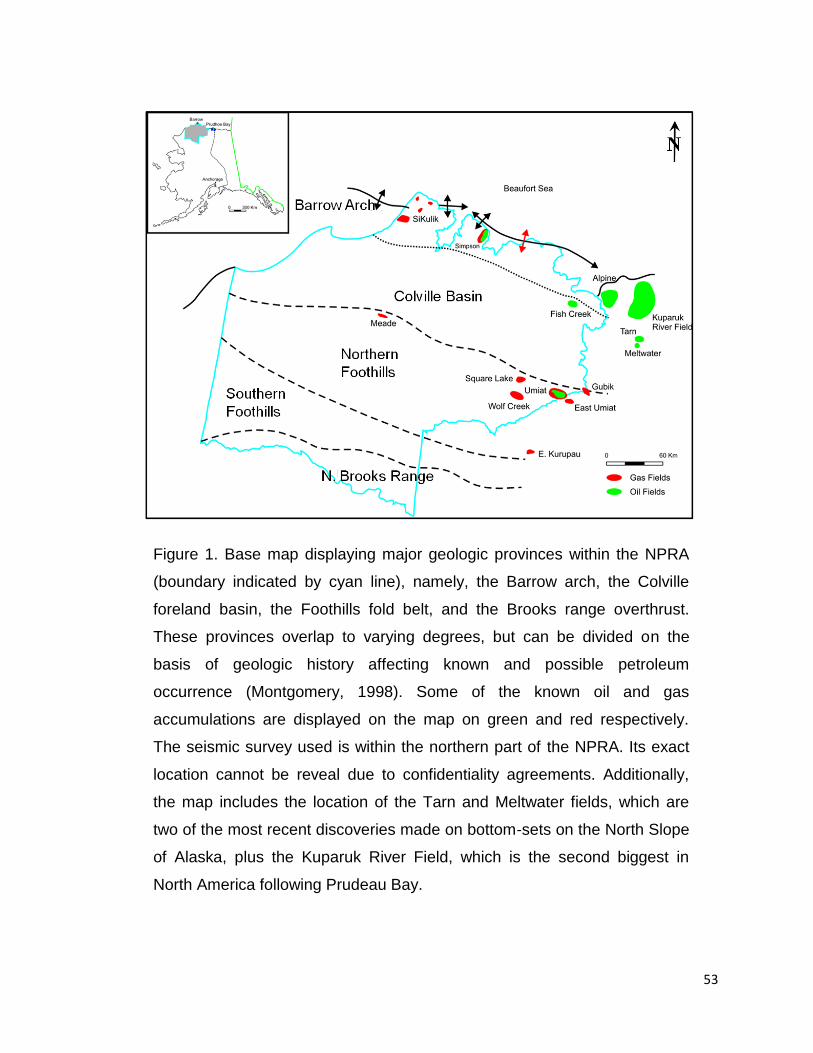
53
Figure 1. Base map displaying major geologic provinces within the NPRA
(boundary indicated by cyan line), namely, the Barrow arch, the Colville
foreland basin, the Foothills fold belt, and the Brooks range overthrust.
These provinces overlap to varying degrees, but can be divided on the
basis of geologic history affecting known and possible petroleum
occurrence (Montgomery, 1998). Some of the known oil and gas
accumulations are displayed on the map on green and red respectively.
The seismic survey used is within the northern part of the NPRA. Its exact
location cannot be reveal due to confidentiality agreements. Additionally,
the map includes the location of the Tarn and Meltwater fields, which are
two of the most recent discoveries made on bottom-sets on the North Slope
of Alaska, plus the Kuparuk River Field, which is the second biggest in
North America following Prudeau Bay.
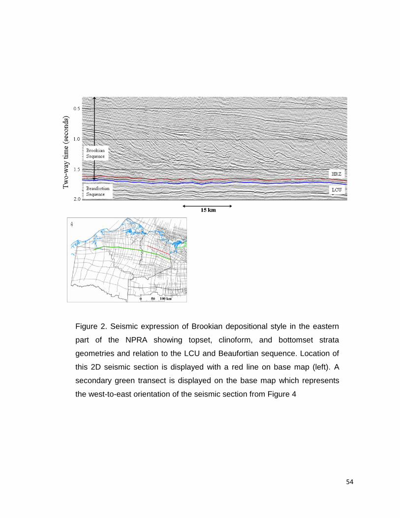
54
Figure 2. Seismic expression of Brookian depositional style in the eastern
part of the NPRA showing topset, clinoform, and bottomset strata
geometries and relation to the LCU and Beaufortian sequence. Location of
this 2D seismic section is displayed with a red line on base map (left). A
secondary green transect is displayed on the base map which represents
the west-to-east orientation of the seismic section from Figure 4
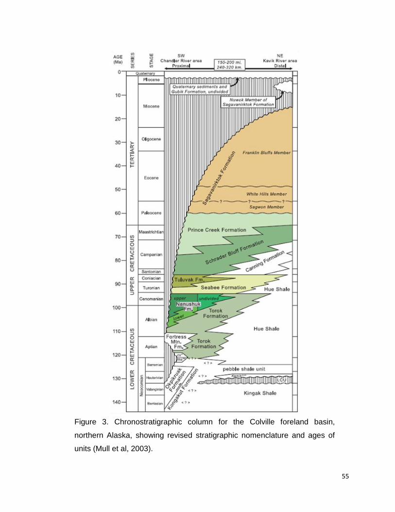
55
Figure 3. Chronostratigraphic column for the Colville foreland basin,
northern Alaska, showing revised stratigraphic nomenclature and ages of
units (Mull et al, 2003).
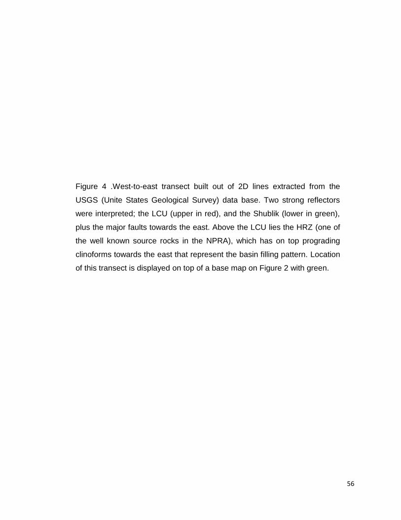
56
Figure 4 .West-to-east transect built out of 2D lines extracted from the
USGS (Unite States Geological Survey) data base. Two strong reflectors
were interpreted; the LCU (upper in red), and the Shublik (lower in green),
plus the major faults towards the east. Above the LCU lies the HRZ (one of
the well known source rocks in the NPRA), which has on top prograding
clinoforms towards the east that represent the basin filling pattern. Location
of this transect is displayed on top of a base map on Figure 2 with green.
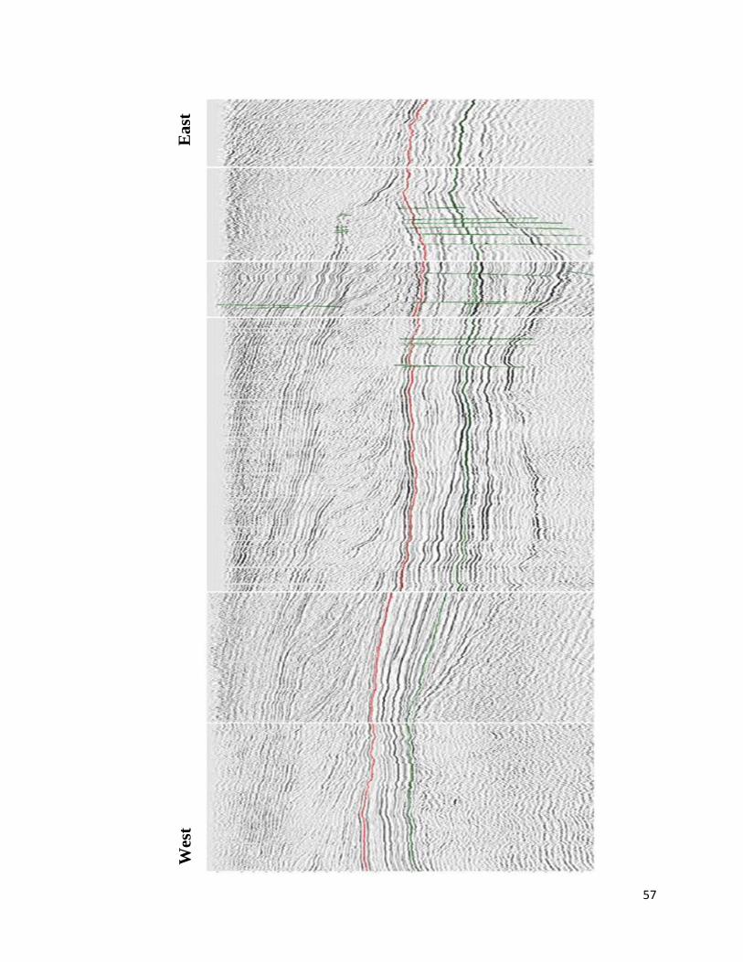
57
Wes
t E
ast
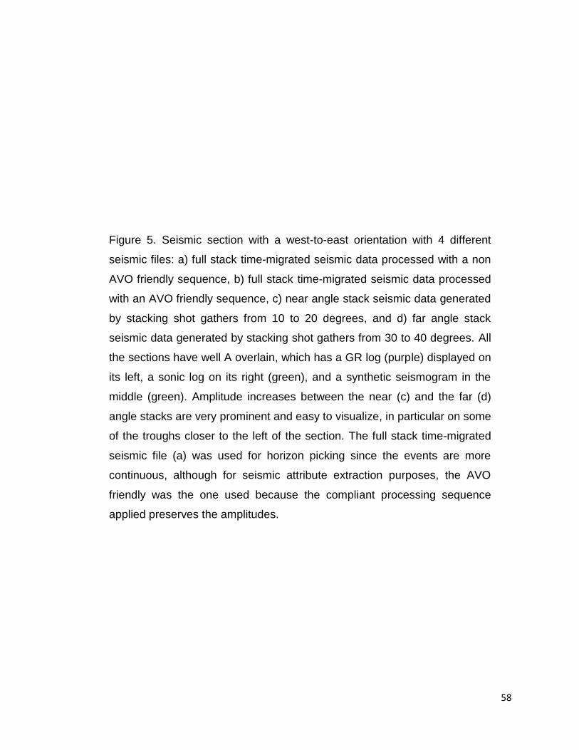
58
Figure 5. Seismic section with a west-to-east orientation with 4 different
seismic files: a) full stack time-migrated seismic data processed with a non
AVO friendly sequence, b) full stack time-migrated seismic data processed
with an AVO friendly sequence, c) near angle stack seismic data generated
by stacking shot gathers from 10 to 20 degrees, and d) far angle stack
seismic data generated by stacking shot gathers from 30 to 40 degrees. All
the sections have well A overlain, which has a GR log (purple) displayed on
its left, a sonic log on its right (green), and a synthetic seismogram in the
middle (green). Amplitude increases between the near (c) and the far (d)
angle stacks are very prominent and easy to visualize, in particular on some
of the troughs closer to the left of the section. The full stack time-migrated
seismic file (a) was used for horizon picking since the events are more
continuous, although for seismic attribute extraction purposes, the AVO
friendly was the one used because the compliant processing sequence
applied preserves the amplitudes.
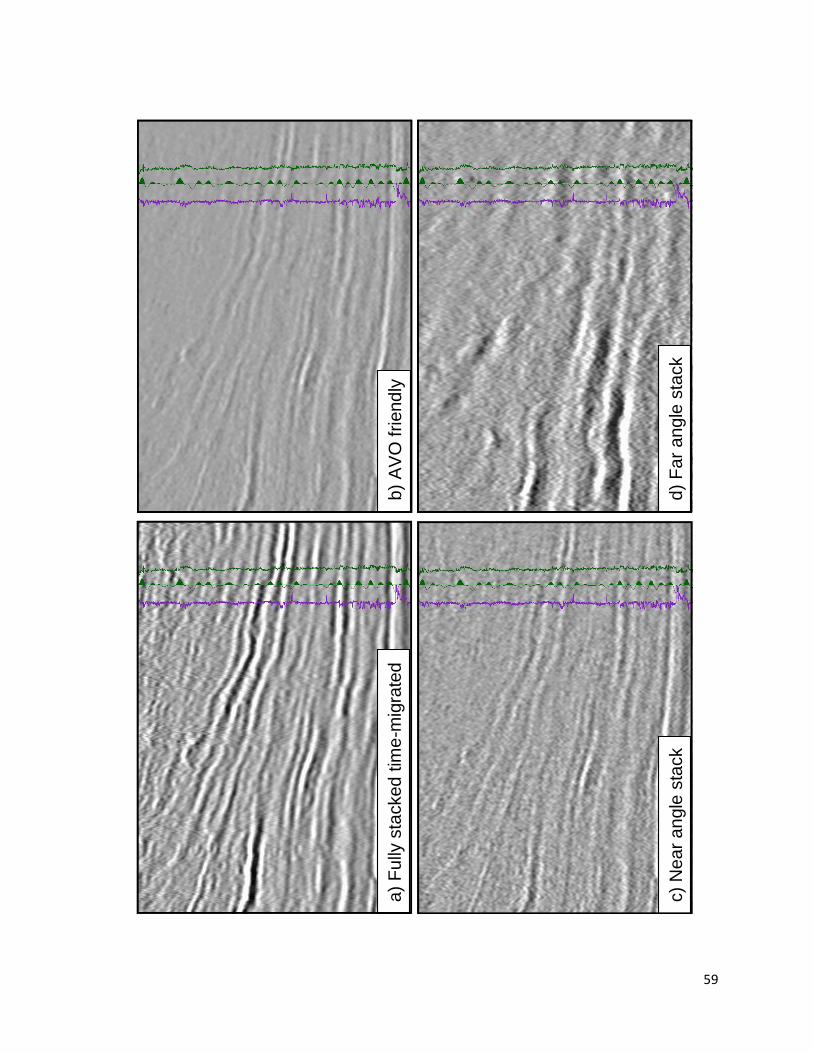
59
a)
Fully
sta
cked t
ime
-mig
rate
db)
AV
O f
riendly
c)
Nea
r an
gle
sta
ck
d)
Far
angle
sta
ck
a)
Fully
sta
cked t
ime
-mig
rate
db)
AV
O f
riendly
c)
Nea
r an
gle
sta
ck
d)
Far
angle
sta
ck
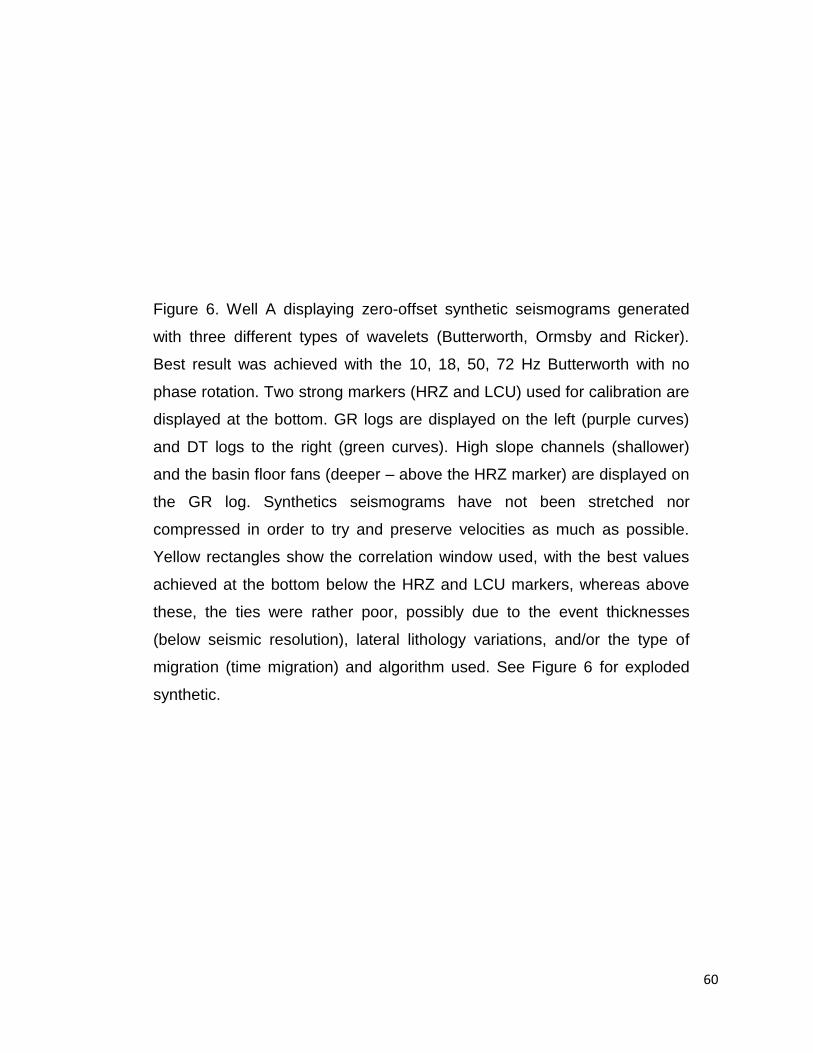
60
Figure 6. Well A displaying zero-offset synthetic seismograms generated
with three different types of wavelets (Butterworth, Ormsby and Ricker).
Best result was achieved with the 10, 18, 50, 72 Hz Butterworth with no
phase rotation. Two strong markers (HRZ and LCU) used for calibration are
displayed at the bottom. GR logs are displayed on the left (purple curves)
and DT logs to the right (green curves). High slope channels (shallower)
and the basin floor fans (deeper – above the HRZ marker) are displayed on
the GR log. Synthetics seismograms have not been stretched nor
compressed in order to try and preserve velocities as much as possible.
Yellow rectangles show the correlation window used, with the best values
achieved at the bottom below the HRZ and LCU markers, whereas above
these, the ties were rather poor, possibly due to the event thicknesses
(below seismic resolution), lateral lithology variations, and/or the type of
migration (time migration) and algorithm used. See Figure 6 for exploded
synthetic.
61
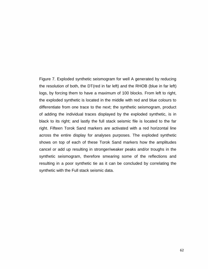
62
Figure 7. Exploded synthetic seismogram for well A generated by reducing
the resolution of both, the DT(red in far left) and the RHOB (blue in far left)
logs, by forcing them to have a maximum of 100 blocks. From left to right,
the exploded synthetic is located in the middle with red and blue colours to
differentiate from one trace to the next; the synthetic seismogram, product
of adding the individual traces displayed by the exploded synthetic, is in
black to its right; and lastly the full stack seismic file is located to the far
right. Fifteen Torok Sand markers are activated with a red horizontal line
across the entire display for analyses purposes. The exploded synthetic
shows on top of each of these Torok Sand markers how the amplitudes
cancel or add up resulting in stronger/weaker peaks and/or troughs in the
synthetic seismogram, therefore smearing some of the reflections and
resulting in a poor synthetic tie as it can be concluded by correlating the
synthetic with the Full stack seismic data.
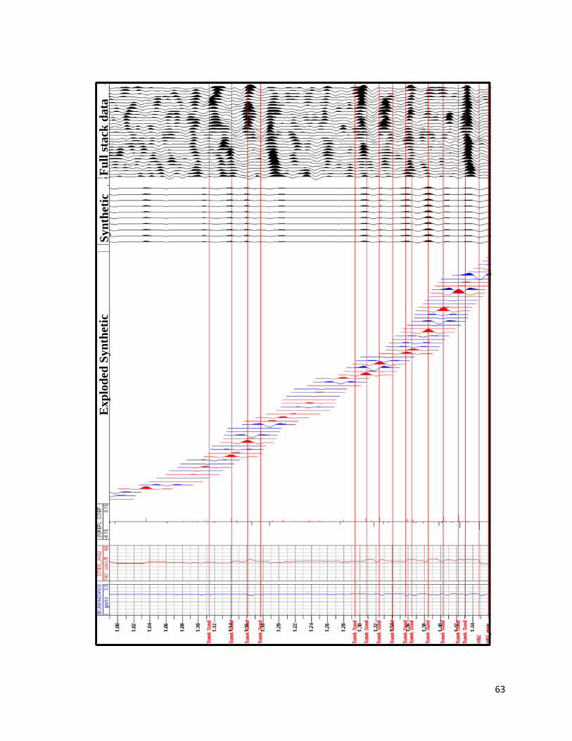
63
F
ull
sta
ck d
ata
E
xp
lod
ed
Sy
nth
etic
S
yn
thet
ic
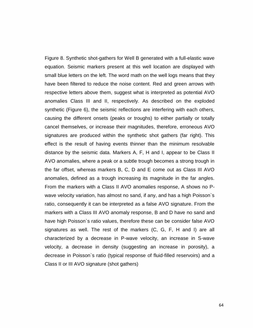
64
Figure 8. Synthetic shot-gathers for Well B generated with a full-elastic wave
equation. Seismic markers present at this well location are displayed with
small blue letters on the left. The word math on the well logs means that they
have been filtered to reduce the noise content. Red and green arrows with
respective letters above them, suggest what is interpreted as potential AVO
anomalies Class III and II, respectively. As described on the exploded
synthetic (Figure 6), the seismic reflections are interfering with each others,
causing the different onsets (peaks or troughs) to either partially or totally
cancel themselves, or increase their magnitudes, therefore, erroneous AVO
signatures are produced within the synthetic shot gathers (far right). This
effect is the result of having events thinner than the minimum resolvable
distance by the seismic data. Markers A, F, H and I, appear to be Class II
AVO anomalies, where a peak or a subtle trough becomes a strong trough in
the far offset, whereas markers B, C, D and E come out as Class III AVO
anomalies, defined as a trough increasing its magnitude in the far angles.
From the markers with a Class II AVO anomalies response, A shows no P-
wave velocity variation, has almost no sand, if any, and has a high Poisson`s
ratio, consequently it can be interpreted as a false AVO signature. From the
markers with a Class III AVO anomaly response, B and D have no sand and
have high Poisson`s ratio values, therefore these can be consider false AVO
signatures as well. The rest of the markers (C, G, F, H and I) are all
characterized by a decrease in P-wave velocity, an increase in S-wave
velocity, a decrease in density (suggesting an increase in porosity), a
decrease in Poisson`s ratio (typical response of fluid-filled reservoirs) and a
Class II or III AVO signature (shot gathers)
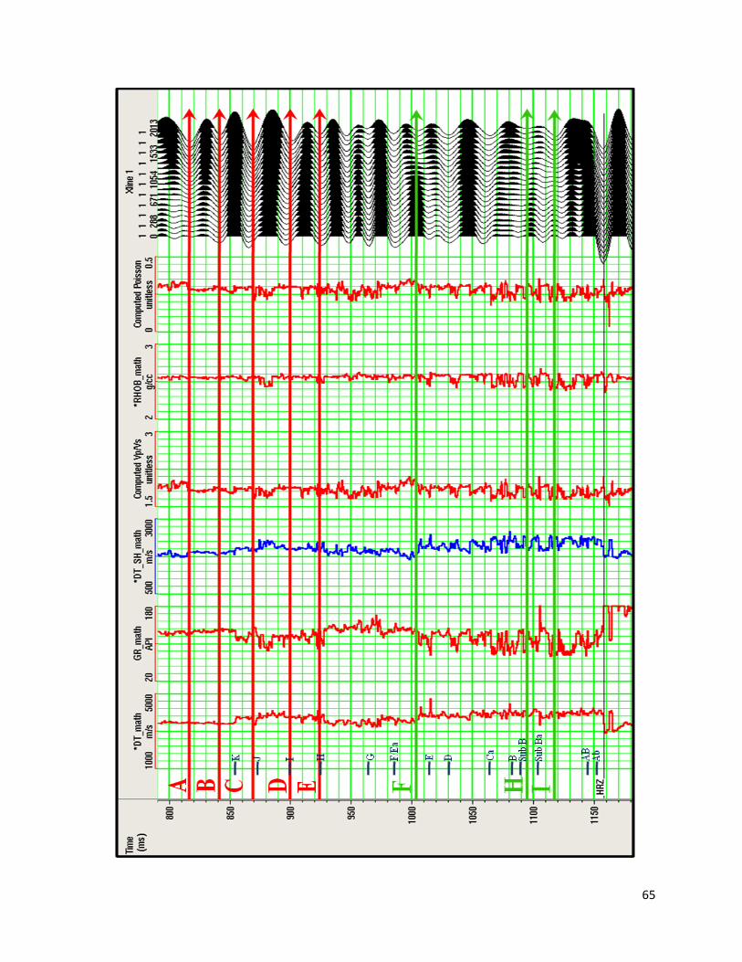
65
66
Figure 9. Seismic section with Well A displayed on top of the fully stacked
time-migrated seismic data (not AVO friendly). The well has displayed a GR
log (left), a DT log (right), and a synthetic seismogram (center). These logs
together show the seismic character of 17 of the main interpreted markers.
The lower portion of the GR (above the HRZ up to Torok E) shows
interbedded sands with shales that represent the lower fan system, whereas
above this interval, the present sands correspond to high slope channels. As
the GR shows, the thickness of some of these sands at this well location are
considerably below the seismic resolution, making it impossible to map as
individual packages, so they were mapped as groups between the two same
most proximal onset types (e.g. from trough to trough). As explained with the
exploded synthetic (Figure 6), the well-to-seismic ties above the HRZ are
poor due to unresolvable events by the seismic data, time-migration and
algorithm applied, AVO anomalies present, and lateral lithology variations
due to the deposition environment (turbidites/basin floor fans).
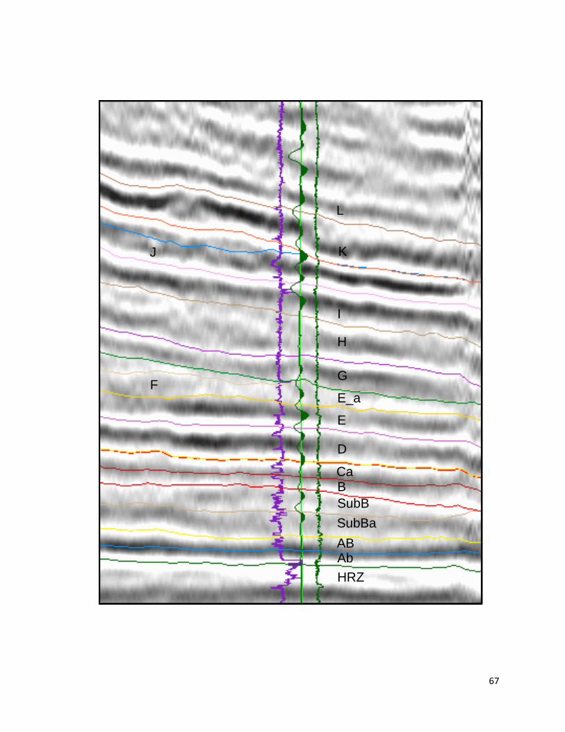
67
HRZ
AbAB
SubBa
SubB
B Ca
D
E
E_aF
G
H
I
J K
L
HRZ
AbAB
SubBa
SubB
B Ca
D
E
E_aF
G
H
I
J K
L
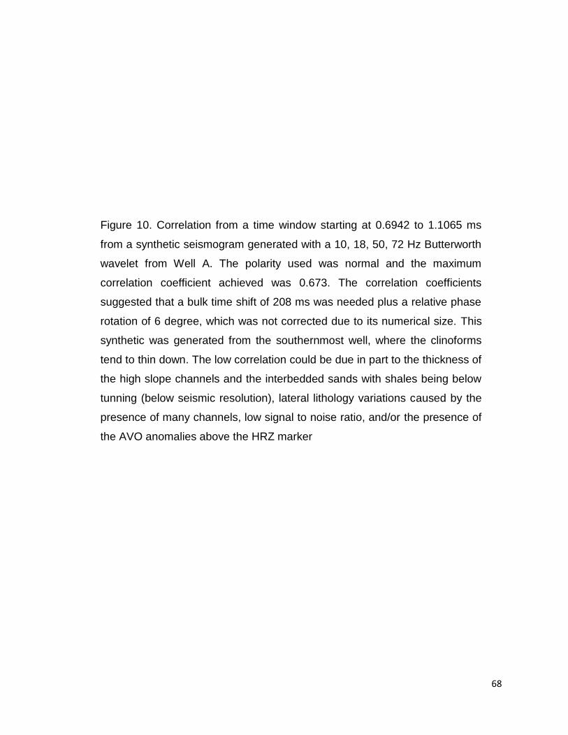
68
Figure 10. Correlation from a time window starting at 0.6942 to 1.1065 ms
from a synthetic seismogram generated with a 10, 18, 50, 72 Hz Butterworth
wavelet from Well A. The polarity used was normal and the maximum
correlation coefficient achieved was 0.673. The correlation coefficients
suggested that a bulk time shift of 208 ms was needed plus a relative phase
rotation of 6 degree, which was not corrected due to its numerical size. This
synthetic was generated from the southernmost well, where the clinoforms
tend to thin down. The low correlation could be due in part to the thickness of
the high slope channels and the interbedded sands with shales being below
tunning (below seismic resolution), lateral lithology variations caused by the
presence of many channels, low signal to noise ratio, and/or the presence of
the AVO anomalies above the HRZ marker
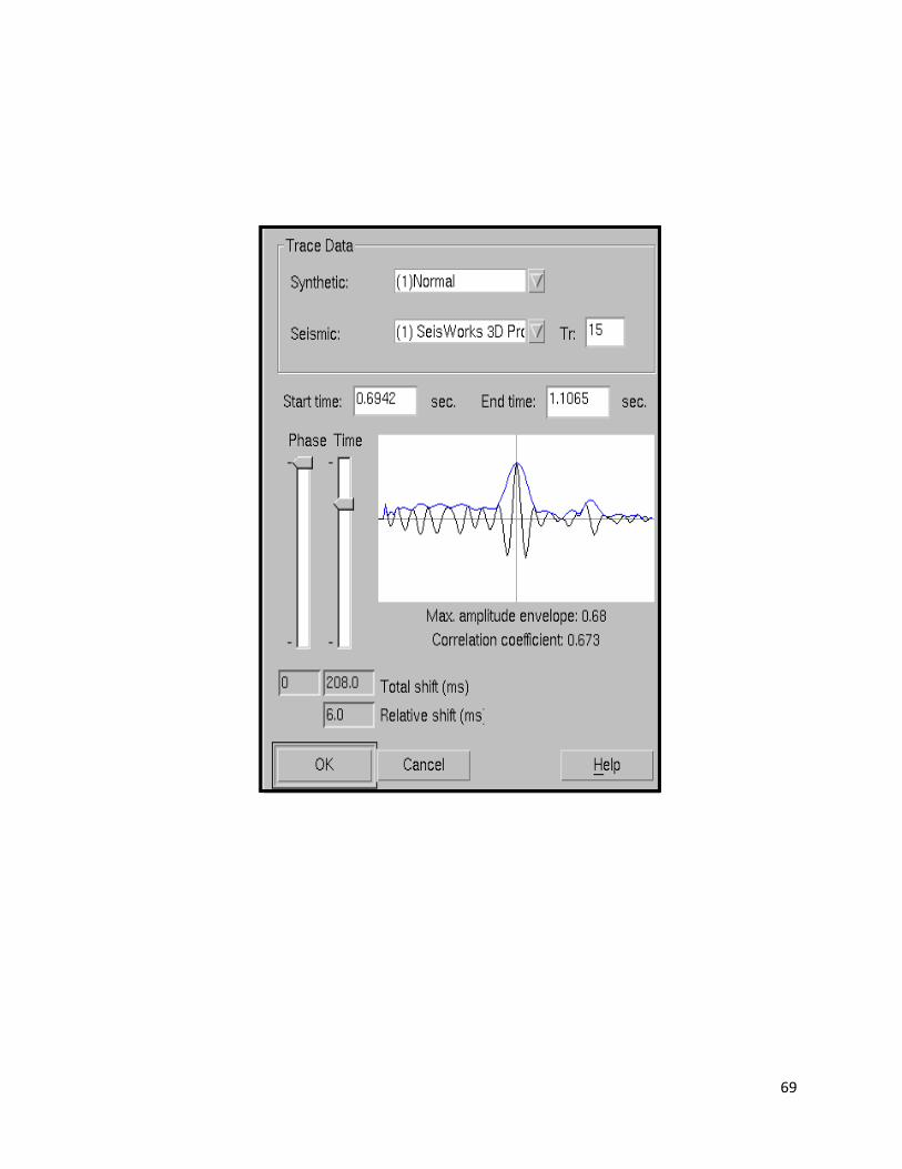
69
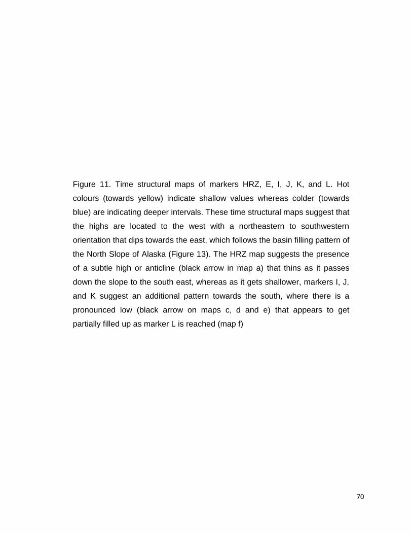
70
Figure 11. Time structural maps of markers HRZ, E, I, J, K, and L. Hot
colours (towards yellow) indicate shallow values whereas colder (towards
blue) are indicating deeper intervals. These time structural maps suggest that
the highs are located to the west with a northeastern to southwestern
orientation that dips towards the east, which follows the basin filling pattern of
the North Slope of Alaska (Figure 13). The HRZ map suggests the presence
of a subtle high or anticline (black arrow in map a) that thins as it passes
down the slope to the south east, whereas as it gets shallower, markers I, J,
and K suggest an additional pattern towards the south, where there is a
pronounced low (black arrow on maps c, d and e) that appears to get
partially filled up as marker L is reached (map f)
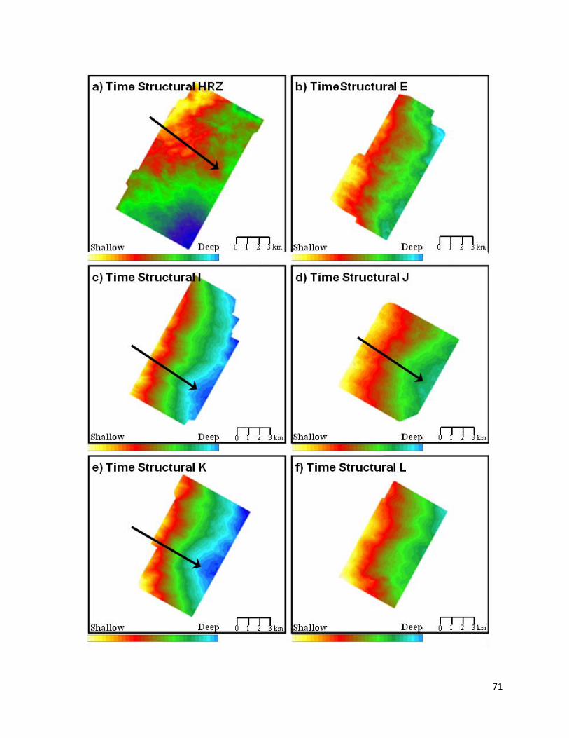
71
72
Figure 12. Composite of isochrons where the base of each map corresponds
to the HRZ, the top or shallower markers are surfaces that get younger in
age starting with marker G (a) all the way to marker L (f). Color bars used are
the same for the six maps, with red to yellow displaying shallow values, and
dark blue representing deeper contours. This set of maps clearly show the
west-to-east depositional filling pattern reflected by contours with an
approximate south-to-north trend and an east dip that indicates the filling
pattern over the slope towards the basin as the seismic transect from Figure
4 also suggests. Isochrons for intervals H, I, J, K, and L suggest the
presence of a low (black arrow in each map), easily recognized with the
white trend line between the yellow and light blue colors. This low could
potentially be a good location for sediment deposits that were carried by
currents down the slope
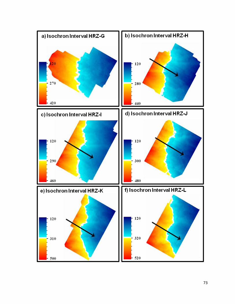
73
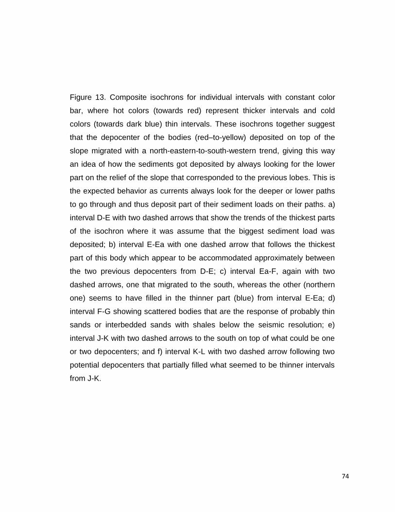
74
Figure 13. Composite isochrons for individual intervals with constant color
bar, where hot colors (towards red) represent thicker intervals and cold
colors (towards dark blue) thin intervals. These isochrons together suggest
that the depocenter of the bodies (red–to-yellow) deposited on top of the
slope migrated with a north-eastern-to-south-western trend, giving this way
an idea of how the sediments got deposited by always looking for the lower
part on the relief of the slope that corresponded to the previous lobes. This is
the expected behavior as currents always look for the deeper or lower paths
to go through and thus deposit part of their sediment loads on their paths. a)
interval D-E with two dashed arrows that show the trends of the thickest parts
of the isochron where it was assume that the biggest sediment load was
deposited; b) interval E-Ea with one dashed arrow that follows the thickest
part of this body which appear to be accommodated approximately between
the two previous depocenters from D-E; c) interval Ea-F, again with two
dashed arrows, one that migrated to the south, whereas the other (northern
one) seems to have filled in the thinner part (blue) from interval E-Ea; d)
interval F-G showing scattered bodies that are the response of probably thin
sands or interbedded sands with shales below the seismic resolution; e)
interval J-K with two dashed arrows to the south on top of what could be one
or two depocenters; and f) interval K-L with two dashed arrow following two
potential depocenters that partially filled what seemed to be thinner intervals
from J-K.
75
76
Figure 14. Wireline logs corresponding to Well A with seismic markers J
(green), I (red) and HRZ (blue) displayed. Two cut-off values were applied; a
first one of 120 to indicate sandstones (yellow) on the GR, and a second of
10 ohm.m on the resistivity logs (red vertical line) to indicate potential
hydrocarbon presence or fresh water sandstones. Marker J corresponds to
the top of a relatively thin sandstone package (low GR reading) which is
characterized by a increase in P-wave (DT), a decrease on the S-wave
(DT_SH), a decrease in density (RHOB), and an increase in resistivity,
normally interpreted as a hydrocarbon indicator, since hydrocarbons, as the
rock‟s matrix, are not-conductive, therefore, as the hydrocarbon saturation of
the pores increases, the rock‟s resistivity also is expected to increase.
Marker I represents potentially the base of a thin sandstone, but in this case
this pick is characterized by basically no changes on P nor S-waves, a
relatively small decrease on density but no increase on resistivity, suggesting
no hydrocarbon saturation
77
J
I
HRZ
78
Figure 15. Composite image of seismic marker J (horizon J on Figure 8 close
to AVO signature marker C); a) West-to-east section from the fully stack
time-migrated seismic file is displayed with Well A overlain. Additionally, a
GR (left), a synthetic seismogram (middle), and a sonic log (right) are
displayed for further interpretation. The GR log defines marker J as the
closest seismic marker to the top of a sandstone characterized by a
decrease in the P-wave velocity; b) time structural map (upper middle) with
hot colours (towards yellow) representing shallower values, and cold colours
(towards blue) representing deeper values. Map is showing the orientation of
the slope with a set of arrows pointing at lows that could be interpreted as
feeders with some high slope channels developing down the slope towards
the basin; c) corresponds to the maximum trough amplitude extracted from
the fully stacked seismic file (AVO friendly). Color bar shows low amplitudes
in black and high amplitudes in red. The high amplitude values define
potential high slope channels that appear to form fans/lobes like features
down the slope towards the basins (right); d) and e), correspond to the
maximum trough amplitudes extracted from the near (NAS) and the far angle
stacks (FAS), respectively, both with color bars that define low maximum
trough values in black and high maximum trough values in red. Furthermore,
the difference between FAS and NAS was calculated (f). This variation
corresponds to the absolute increase in amplitude that was interpreted from
the AVO signatures from the synthetic shot gathers (Figure 8), which we will
call, for the purpose of the analysis, “sweet spots”. The color bar for this map
(f) shows in light brown and dark blue, the lowest amplitude differences,
which in this case can be interpreted to be the calculated attribute from bad
manual picking or noise that was incorporated inside of the attribute analysis
time window, therefore only the highest amplitude (lighter blue), are
considered as potential sweet spots.
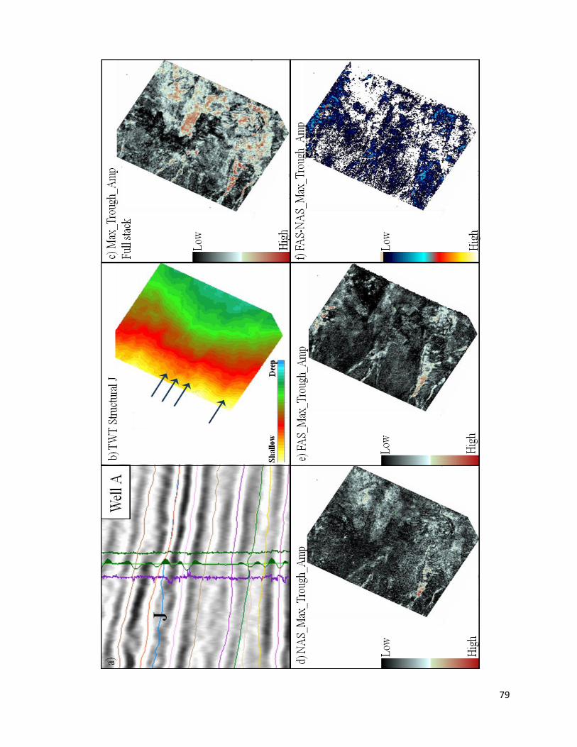
79
80
Figure 16. Composite image of seismic marker J (horizon J close to AVO
signature marker C) showing two complex trace attribute analyses (see
Appendix A for complex trace attribute analysis theory), average reflection
strength (a, b and c maps), also known as envelope amplitude, and the total
energy (d, e, and f maps). Both attributes were extracted from the NAS and
FAS, and additionally, the difference between the FAS and the NAS was
calculated (c and f ) as for the maximum trough amplitude on Figure 14. The
color bars for the NAS and FAS define low amplitudes as colours towards
black and high amplitude as colours towards red. The NAS maps (a and d)
roughly define what can be interpreted as a high slope channel system, with
most of these channel like features suggesting a steep slope due to their
almost straight trend. The FAS (b and e) sharpen the amplitudes that define
some of these events. This was an expected response from the modeling
results (Figure 8), maximum trough amplitude analysis (Figure 15), and also
an anticipated response from the Alaskan sandstones with Class II to III AVO
anomalies. Maps c) and f) show the calculated difference between the FAS
and the NAS (potential sweet spots), and as indicated by the color bars, the
light brown colours correspond to the lowest amplitude differences, which as
for the maximum trough amplitude case, are considered the results of bad
manual picking or noise that comes in from the time window used to extract
these attributes, therefore only the highest differences (blue features
following the high slope channel features trend) are considered sweet spots
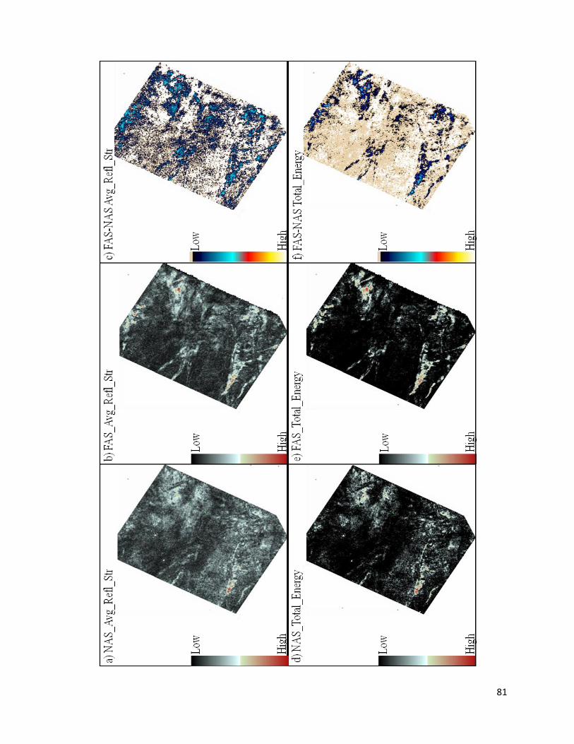
81
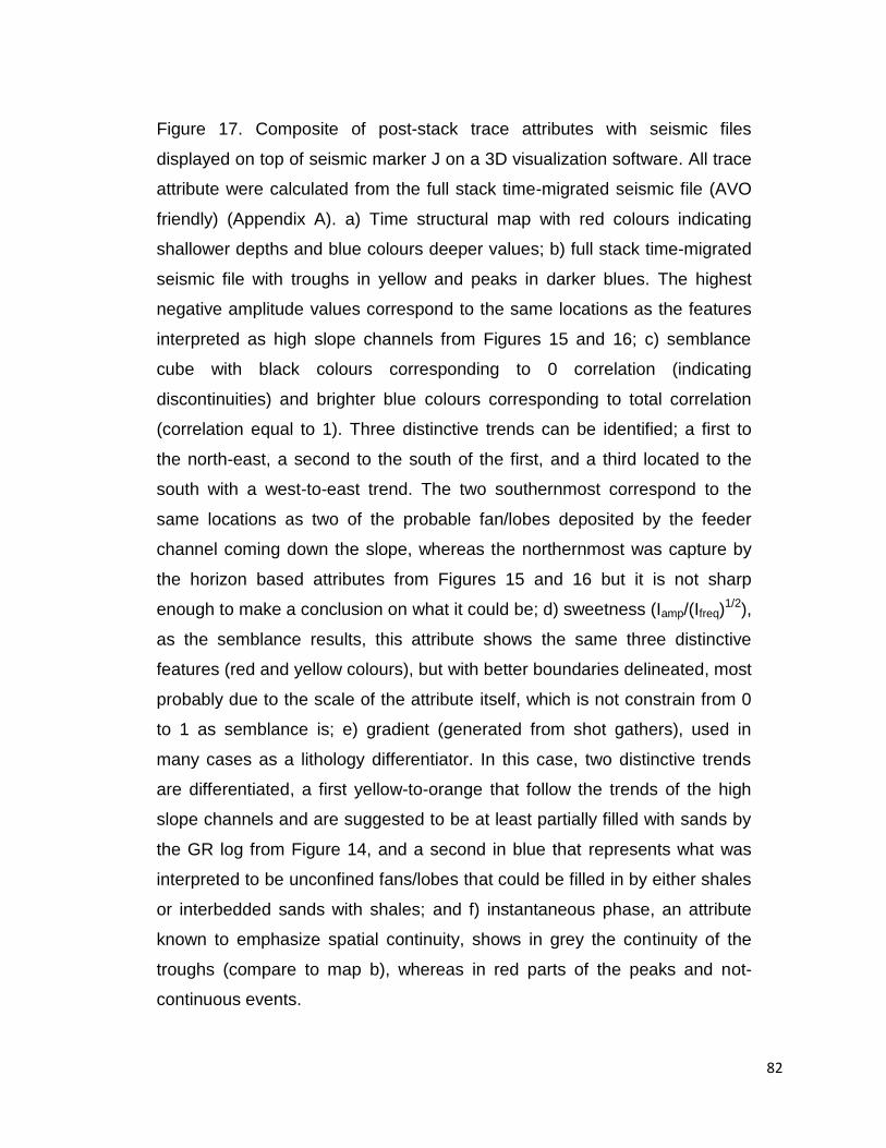
82
Figure 17. Composite of post-stack trace attributes with seismic files
displayed on top of seismic marker J on a 3D visualization software. All trace
attribute were calculated from the full stack time-migrated seismic file (AVO
friendly) (Appendix A). a) Time structural map with red colours indicating
shallower depths and blue colours deeper values; b) full stack time-migrated
seismic file with troughs in yellow and peaks in darker blues. The highest
negative amplitude values correspond to the same locations as the features
interpreted as high slope channels from Figures 15 and 16; c) semblance
cube with black colours corresponding to 0 correlation (indicating
discontinuities) and brighter blue colours corresponding to total correlation
(correlation equal to 1). Three distinctive trends can be identified; a first to
the north-east, a second to the south of the first, and a third located to the
south with a west-to-east trend. The two southernmost correspond to the
same locations as two of the probable fan/lobes deposited by the feeder
channel coming down the slope, whereas the northernmost was capture by
the horizon based attributes from Figures 15 and 16 but it is not sharp
enough to make a conclusion on what it could be; d) sweetness (Iamp/(Ifreq)1/2),
as the semblance results, this attribute shows the same three distinctive
features (red and yellow colours), but with better boundaries delineated, most
probably due to the scale of the attribute itself, which is not constrain from 0
to 1 as semblance is; e) gradient (generated from shot gathers), used in
many cases as a lithology differentiator. In this case, two distinctive trends
are differentiated, a first yellow-to-orange that follow the trends of the high
slope channels and are suggested to be at least partially filled with sands by
the GR log from Figure 14, and a second in blue that represents what was
interpreted to be unconfined fans/lobes that could be filled in by either shales
or interbedded sands with shales; and f) instantaneous phase, an attribute
known to emphasize spatial continuity, shows in grey the continuity of the
troughs (compare to map b), whereas in red parts of the peaks and not-
continuous events.
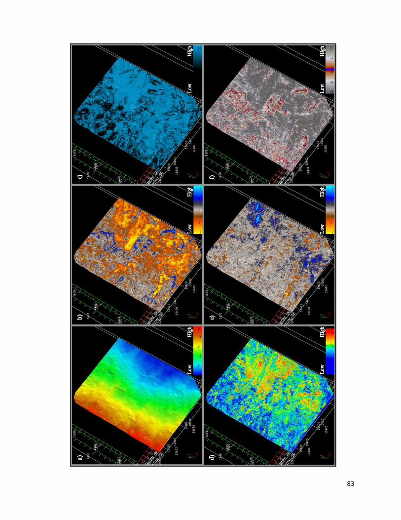
83
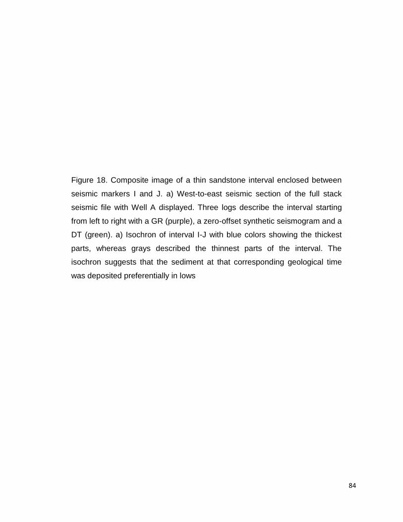
84
Figure 18. Composite image of a thin sandstone interval enclosed between
seismic markers I and J. a) West-to-east seismic section of the full stack
seismic file with Well A displayed. Three logs describe the interval starting
from left to right with a GR (purple), a zero-offset synthetic seismogram and a
DT (green). a) Isochron of interval I-J with blue colors showing the thickest
parts, whereas grays described the thinnest parts of the interval. The
isochron suggests that the sediment at that corresponding geological time
was deposited preferentially in lows
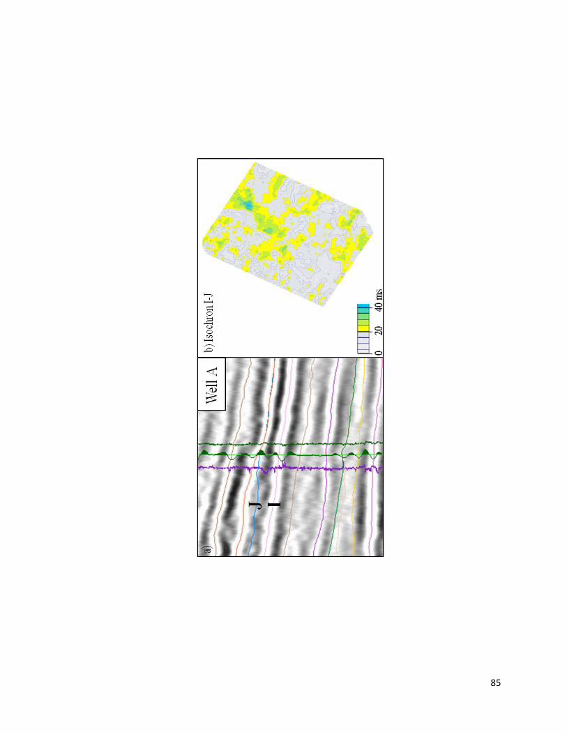
85
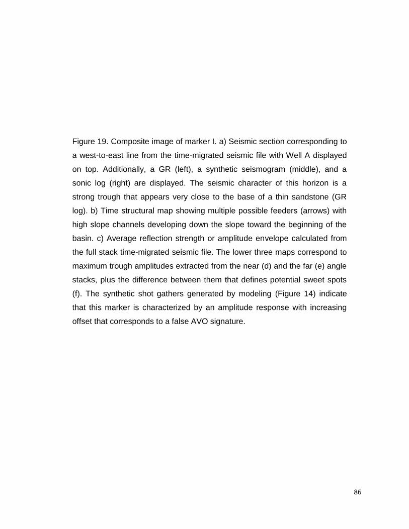
86
Figure 19. Composite image of marker I. a) Seismic section corresponding to
a west-to-east line from the time-migrated seismic file with Well A displayed
on top. Additionally, a GR (left), a synthetic seismogram (middle), and a
sonic log (right) are displayed. The seismic character of this horizon is a
strong trough that appears very close to the base of a thin sandstone (GR
log). b) Time structural map showing multiple possible feeders (arrows) with
high slope channels developing down the slope toward the beginning of the
basin. c) Average reflection strength or amplitude envelope calculated from
the full stack time-migrated seismic file. The lower three maps correspond to
maximum trough amplitudes extracted from the near (d) and the far (e) angle
stacks, plus the difference between them that defines potential sweet spots
(f). The synthetic shot gathers generated by modeling (Figure 14) indicate
that this marker is characterized by an amplitude response with increasing
offset that corresponds to a false AVO signature.
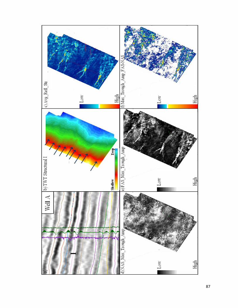
87

88
Figure 20. Composite of two similar amplitude statistic seismic attribute
maps, RMS amplitude and total energy. The upper maps correspond to RMS
calculated from near (a) and far (b) angle stacks, plus the difference between
them (c), whereas the lower correspond to total energy calculated from the
same angle stacks. The far minus the near angle stacks (offset) define the
difference in amplitude with increasing offset, which according to the
synthetic shot gathers correspond to amplitude responses that correspond to
seismic background. Color bars for the total energy (d, e, and f) outputs
where adjusted in order to sharpen the false AVO signatures described in the
far angles.
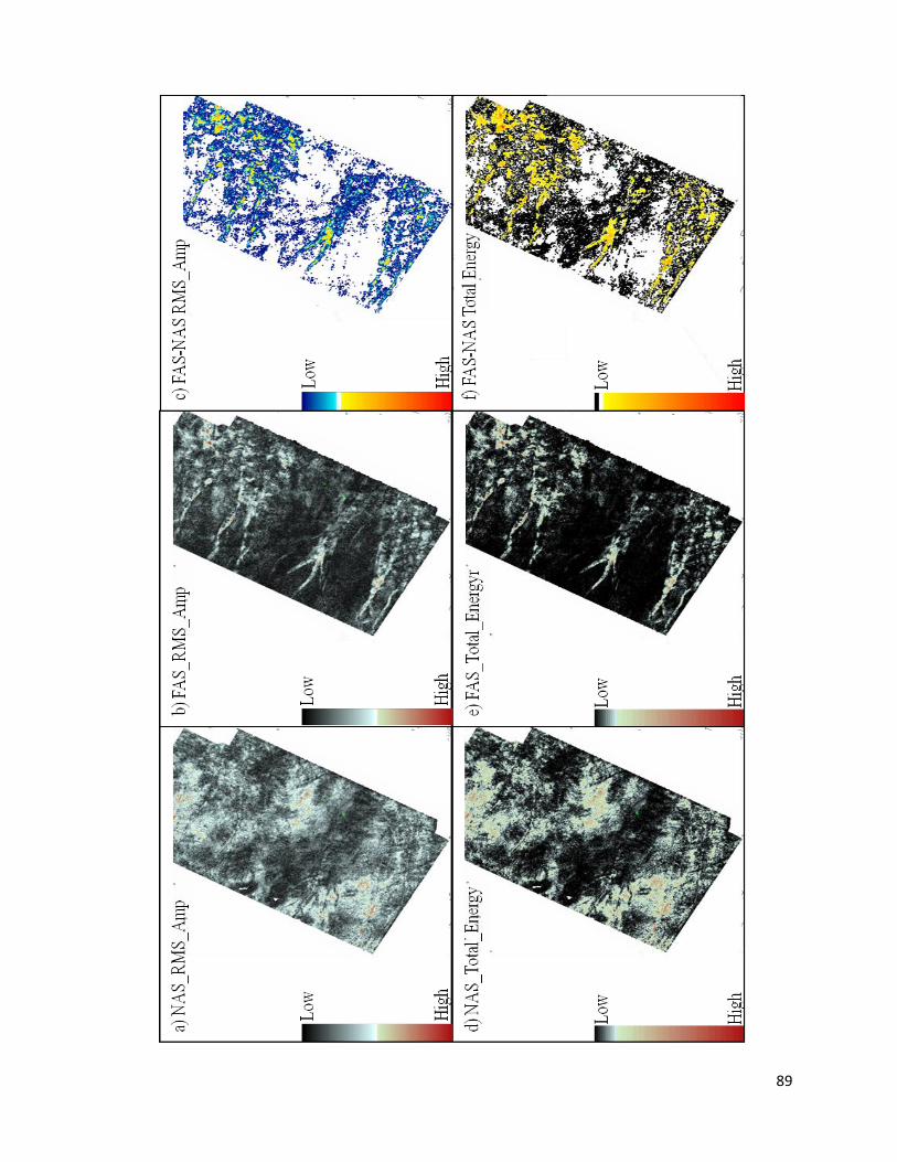
89
90
Figure 21. Summary of RMS amplitudes of randomly selected markers within
the Torok Formation calculated from far angle stacks (FAS) to isolate the
amplitude responses with increasing offset. By isolating these responses
from the FAS, amplitude responses with increasing offset that define possible
deep water geomorphologies can be better analyzed due to their increased
sharpness. Some of these responses are what characterize AVO anomalies
Class II and III, although before classifying them it is necessary to analyze
the synthetic shot gathers acquired from the AVO modeling (Figure 8)
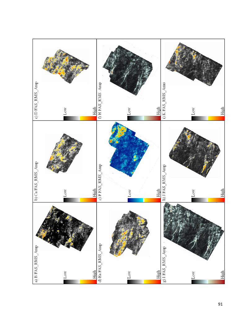
91

92
Figure 22. Summary of the differences between maximum trough amplitude
calculated from the far and near angle stack seismic files from randomly
selected markers within the Torok Formation. Normally, when in the
presence of Class II or III AVO anomalies, the difference between attributes
calculated from far and near angle stacks will define the sweet spots or
bodies with anomalous amplitude, but as it can be seen from either Figure 14
or Table 2, there is always the possibility of obtaining an AVO response from
the seismic background, which can be due to factors such as a shale with a
decrease in P-wave and an increase in S-wave velocity, small porosity
variations, wrong seismic processing sequence applied, and the presence of
volcanic ash, among others
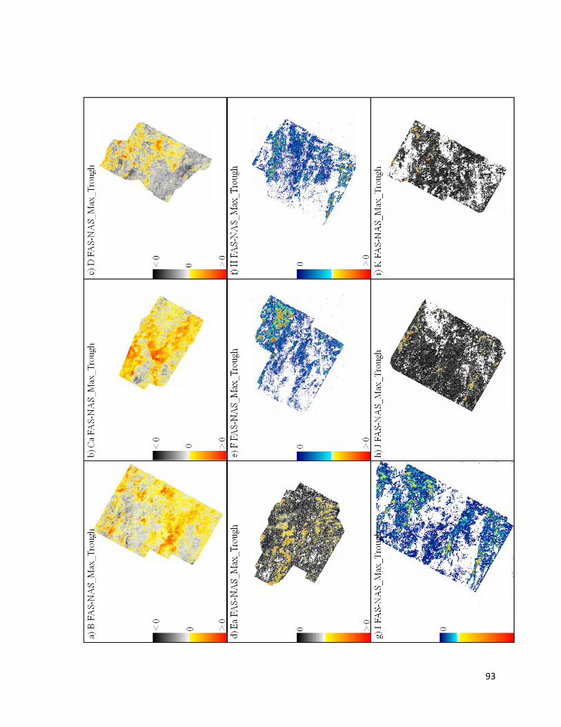
93
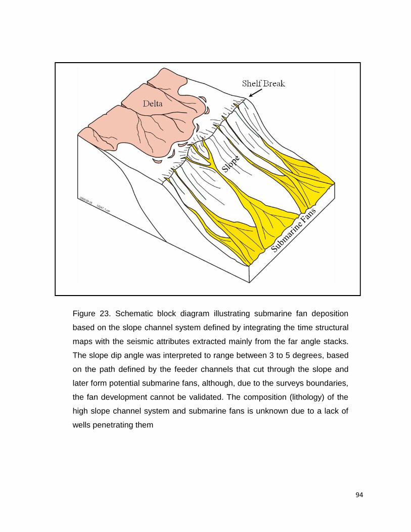
94
Figure 23. Schematic block diagram illustrating submarine fan deposition
based on the slope channel system defined by integrating the time structural
maps with the seismic attributes extracted mainly from the far angle stacks.
The slope dip angle was interpreted to range between 3 to 5 degrees, based
on the path defined by the feeder channels that cut through the slope and
later form potential submarine fans, although, due to the surveys boundaries,
the fan development cannot be validated. The composition (lithology) of the
high slope channel system and submarine fans is unknown due to a lack of
wells penetrating them

95
Table 1. Well data base showing the wireline log availability for each well
used for both the seismic calibration (DT, GR, and RHOB) and the AVO
modeling (DT, DT_SH, GR, and RHOB)
96
Table 2. Classification of the different amplitude responses to increasing
offset based on the elastic modeling results obtained for the three different
wells with S-wave sonics. The classification is done for individual markers
and intervals in cases where sandstone bodies or interbedded sandstones
with shales are present between two horizons. Amplitude responses are
described based on the intercept (starting onset type) and gradient (slope). In
some cases the AVO anomalies observed on both the synthetic shot gathers
and the angle stack files correspond to false anomalies, which could be due
to reflector dip and depth, receiver array attenuation, inelastic attenuation,
thin bed effects, anisotropy and/or an erroneous seismic processing
sequence
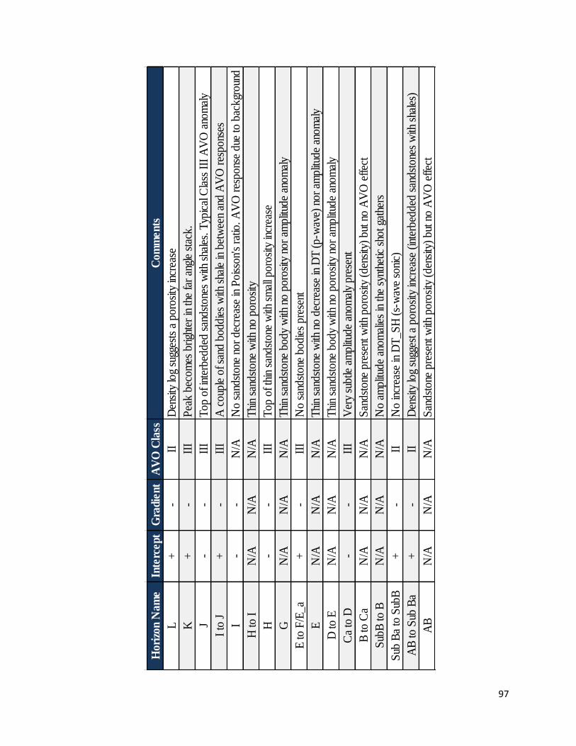
97
Ho
rizo
n N
am
eIn
terc
ept
Gra
die
nt
AV
O C
lass
Co
mm
ents
L+
-II
Den
sity
log
sugg
ests
a p
oro
sity
incr
ease
K+
-II
IP
eak
bec
om
es b
righ
ter
in the
far
ang
le s
tack
.
J-
-II
IT
op
of in
terb
edd
ed s
and
sto
nes
with
sha
les.
Typ
ical
Cla
ss I
II A
VO
ano
mal
y
I to
J+
-II
IA
co
uple
of sa
nd b
od
die
s w
ith s
hale
in b
etw
een
and
AV
O r
esp
ons
es
I-
-N
/AN
o s
and
sto
ne n
or
dec
reas
e in
Po
isso
n's
ratio
. A
VO
res
po
nse
due
to
bac
kgr
oun
d
H to
IN
/AN
/AN
/AT
hin
sand
sto
ne w
ith n
o p
oro
sity
H-
-II
IT
op
of th
in s
and
sto
ne w
ith s
mal
l po
rosi
ty in
crea
se
GN
/AN
/AN
/AT
hin
sand
sto
ne b
ody
with
no
poro
sity
no
r am
plit
ude
ano
mal
y
E to
F/E
_a
+-
III
No
san
dst
one
bo
die
s p
rese
nt
EN
/AN
/AN
/AT
hin
sand
sto
ne w
ith n
o d
ecre
ase
in D
T (
p-w
ave)
no
r am
plit
ude
ano
mal
y
D to
EN
/AN
/AN
/AT
hin
sand
sto
ne b
ody
with
no
poro
sity
no
r am
plit
ude
ano
mal
y
Ca
to D
--
III
Ver
y su
btle
am
plit
ude
ano
mal
y p
rese
nt
B to
Ca
N/A
N/A
N/A
San
dst
one
pre
sent
with
po
rosi
ty (
den
sity
) b
ut n
o A
VO
effec
t
Sub
B to
BN
/AN
/AN
/AN
o a
mp
litud
e an
om
alie
s in
the
syn
thet
ic s
hot ga
ther
s
Sub
Ba
to S
ubB
+-
IIN
o in
crea
se in
DT
_S
H (
s-w
ave
soni
c)
AB
to
Sub
Ba
+-
IID
ensi
ty lo
g su
gges
t a
po
rosi
ty in
crea
se (
inte
rbed
ded
san
dst
one
s w
ith s
hale
s)
AB
N/A
N/A
N/A
San
dst
one
pre
sent
with
po
rosi
ty (
den
sity
) b
ut n
o A
VO
effec
t
98
CHAPTER 3: CONCLUSIONS
The primary objective of this thesis was to identify potential reservoir sands
within the Torok Formation in a southern portion of a 3D survey located in
the Northern Slope of Alaska by integrating complex trace attributes with
AVO modeling. As a result, I successfully subdivided the lower portion of
the Torok Formation into 24 different horizons, which made it possible to
perform a detailed seismic attribute analysis of each seismic marker. By
modeling synthetic shot gathers using a fully elastic wave equation, Class II
and III AVO anomalies where identified; the first (Class II) were defined by a
positive or very subtle negative intercept and a negative gradient, and the
last (Class III) were described by a negative intercept and gradient.
By acquiring amplitude and complex trace attributes from the near and far
angle stack seismic files, it was possible to map and capture the
approximate extensions of some of these anomalies considered to be
sweet spots. The integration with wireline logs resulted with seismic
markers J, K and L, and intervals AB-to-Sub Ba, Sub Ba-to-SubB, Ca-to-D,
and E-to-F/Ea as the most prospective due to a suggested increase in
porosity (suggested by a decrease in density log values), a decrease in the
P-wave velocity, an increase in the S-wave velocity, a decrease in
Poisson‟s ratio (characteristic response of fluid filled reservoirs) and an
increase in resistivity (characteristic hydrocarbon response). Some of the
prospective markers delineated the geomorphology of a high slope channel
system close to the shelf edge, which presumably transported sediments
down the slope, and would end up accumulating them further down as
fans/lobes filled up with either sands or interbedded sands with shales.
Some false AVO signatures were identified and mapped, which could have
been caused by seismic signal interference due to events thicknesses
below the seismic resolution, low signal-to-noise ratio (low fold), lithology
lateral variations (anisotropy), and the type of migration algorithm applied to

99
the data, which was not strong enough to entirely correct and move the
events to their real depth.
In addition to defining potential reservoir sand intervals within the Torok Fm,
this study will also help in the further analysis and development of other
prospective areas with similar geological settings within the North Slope of
Alaska by being used as an analogous case study, and by helping to better
understand reservoirs where AVO signatures are present.
100
REFERENCES
Aki, R., Richards P.G., 1980, Quantitative seismology: Theory and
methods: W.H. Freeman and Co., New York.
Barnes, A.E., 1998, The complex seismic trace made simple, The Leading
Edge, Society of Exploration Geophysicists, v. 17, No. 4, p. 473-476.
Barnes, A.E., 2007, A tutorial on complex seismic trace analysis,
Geophysics, Society of Exploration Geophysicists, v. 72, No. 6, p.
W33-W43.
Bird, K. J., and Molenaar, C. M., 1992, The North Slope foreland basin,
Alaska, Foreland basins and fold belts, The American Association of
Petroleum Geologists, Memoir 55, p. 363-393.
Bird, K. J., 1994, The Ellesmerian petroleum system, North Slope of Alaska,
The petroleum system - From source to trap, The American
Association of Petroleum Geologists, Memoir 60, p. 339-358.
Bird, K.J., 2001, Alaska: A Twenty-First –Century Petroleum Province, The
American Association of Petroleum Geologist, Memoir 74, p137-165.
Brown, A.R., 1996, Interpreter‟s Corner - Seismic attributes and their
classification, The Leading Edge, Society of Exploration
Geophysicists, 15, 10, 1090.
Castagna, J.P., 1993, AVO Analysis – Tutorial and Review, Offset-
Dependent Reflectivity–Theory and Practice of AVO Analysis, p. 3-
36.
Castagna, J.P., 1993, Petrophysical imaging using AVO, The Leading
Edge, Society of Exploration Geophysicists, 12, p. 172- 178.
Castagna, J.P., Batzle, M.L., and Kan, T.K., 1995, Rock Physics – The Link
Between Rock Properties and AVO Response, in Castagna, J.P.,
101
and Backus, M.M., Offset-dependent Reflectivity - Theory and
practice of AVO Analysis, Society of Exploration Geophysicists,
Tulsa, OK. p. 135-171.
Castagna, J.P., and Swan, H.W., 1997, Principles of AVO crossplotting,
The Leading Edge, Society of Exploration Geophysicists, 17, p. 337-
342.
Castagna, J.P., Swan, H.W., and Foster, D.J., 1998, Framework for AVO
gradient and intercept interpretation, Geophysics, Society of
Exploration Geophysicists, v. 63, No. 3, p. 948-956.
Chopra, S., 2002, Coherence Cube and beyond, First Break, v. 20.1, p. 27-
33.
Chopra, S., and Marfurt. K. J., 2005, Seismic attributes – A historical
perspective, Geophysics, Society of Exploration Geophysicists, v.
70, No. 5, p. 3-27.
Chopra, S., and Marfurt, K.J., 2007, Seismic Attribute for Prospect
Identification and Reservoir Characterization, ISBN, SEG
Geophysical Developments Series No.11, Chapter 3, p. 45-72.
Claerbout, J.F., 1976, Fundamentals of geophysical data processing,
McGraw-Hill Book Co. Inc.
Cole, F.K., Bird, K.J., Toro, J., Roure, F., O‟Sullivan, P.B., Pawlewicz, M.J.,
and Howell, D.G., 1997, An integrated model for the tectonic
developments of the frontal Brooks Range and Colville Basin 250 km
west of the Trans-Alaska Crustal Transect, Journal of Geophysical
Research, v. 102, No. B9, p. 20685-20708.
Decker, P.L., 2007, Brookian Sequence Stratigraphic Correlations, Umiat
Field to Milne Point Field, West-Central North Slope, Alaska, State of
102
Alaska – Department of Natural Resources, Division of Geological &
Geophysical Surveys, p. 1-19.
Erickson, J. W., and Sneider R. M., 1997, Structural and hydrocarbon
histories of the Ivishak (Sadlerochit) reservoir, Prudhoe Bay field:
SPE Reservoir Engineering, v. 12, p 18-22.
Galloway, W.E., 1998, Siliciclastic Slope and Base-of-Slope Depositional
System: Component Facies, Stratigraphic Architecture, and
Classification, The American Association of Petroleum Geologist, v.
82, No. 4, p. 569-595.
Gingrich, D., Knock, D., and Masters R., 2001, Geophysical interpretation
methods applied at Alpine Oil Field: North Slope, Alaska, The
Leading Edge, Society of Exploration Geophysicists, v. 20, p. 730-
738.
Graul, M., 2001, AVO: Yesterday, Today, and (a peek at) Tomorrow,
Canadian Society of Exploration Geophysicists, Recorder, p. 35-38.
Hart, B., 2008, Channel detection in 3-D seismic data using sweetness, The
American Association of Petroleum Geologist, v. 92, No. 6, p. 733-
742.
Homza, T.X., 2004, A structural interpretation of the Fish Creek Slide
(Lower Cretaceous), northern Alaska, The American Association of
Petroleum Geologists, v. 88, No. 3, p. 265-278.
Houseknecht, D.W., and Schenk, C.J., 2001, Depositional Sequence and
Facies in the Torok Formation, National Petroleum Reserve – Alaska
(NPRA), U. S. Geological Survey, 956, p. 179-199.
Houseknecht, D.W., and Schenk, C.J., 2002, Depositional Sequences and
Facies in the Torok Formation, National Petroleum Reserve – Alaska
(NPRA), U.S. Geological Survey, Core Workshop, p. 5- 26.
103
Hubbanrd, R.J., Edrich, S.P., and Rattey, P.R., 1987, Geologic evolution
and hydrocarbon habitat of the „Arctic Alaska Microplate‟, Marine and
Petroleum Geology, v. 4, p. 2-34
Jamison, H. C., Brockett, L. D., and McIntosh, R. A., 1980, Prudhoe Bay: a
10-year perspective, Giant oil and gas fields of the decade, The
American Association of Petroleum Geologists, Memoir 30, p. 281-
289.
Jones, H. P., and Speers, R. G., 1976, Permo-Triassic reservoirs of
Prudhoe Bay field, North Slope, Alaska, in J. Braunstein ed., North
America oil and gas fields, The American Association of Petroleum
Geologist, Memoir 24, p. 23-50.
Kirschner, C.E., Grantz, A., and Mullen, M.W., 1992, Impact Origin of the
Avak Structure, Arctic Alaska, and Genesis of the Barrow Gas Field,
The American Association of Petroleum Geologists, v. 76, No. 5, p.
651-679.
Kornbrath, R.W., Myers, M.D., Krouskop, D.L., Meyer, J.F., Houle, J.A.,
Ryherd, T.J., and Richter, K.N., 1997, Petroleum Potential of the
Eastern National Petroleum Reserve-Alaska, Alaska Division of Oil
and Gas, p. 1-30.
Li, Y., Downton, J., and Xu, Y., 2007, Practical aspects of AVO modeling,
The Leading Edge, Society of Exploration Geophysicists, v. 26, p.
295-310.
Lillis, P. G., Lewan, M. D., Warden, A., Monk, S. M., and King, J. D, 1999,
Identification and characterization of oil types and their source rocks,
The oil and gas resource potential on the 1002 Area, Arctic National
Wildlife Refuge, Alaska: U.S. Geological Survey Open-File Report
98-34, 2 CD-ROMs, p. OA1-OA56.
104
Magoon, L. B., 1994, The geology of known oil and gas resources by
petroleum system – Onshore Alaska, The geology of Alaska:
Geological Society of America, The geology of North America, v. G-
1, p. 905-936.
Magoon, L. B, and Dow, W. G, eds, 1994, The petroleum system – From
source to trap, The American Association of Petroleum Geologist,
Memoir 60, p. 655.
Magoon, L. B., Bird, K. J., Burruss, R. C., Hayba, D., Houseknecht, D. W.,
Keller, M. A., Lillis, P. G., and Rowan, E. L., 1999, Evaluation of
hydrocarbon charge and timing using the petroleum system, in
ANWR Assessment Team, ed., The oil and gas resource potential of
the 1002 Area, Arctic National Wildlife Refuge, Alaska: U.S.
Geological Survey Open-File Report 98-34, 2 CD-ROMs, p. PS1-
PS66.
Marfurt, K.J., Kirlin, R.L., Farmer, S.L., and Bahorich, M.S., 1998, 3-D
seismic attributes using a semblance-based coherency algorithm,
Geophysics, Society of Exploration Geophysicists, v. 63, p. 1150-
1165.
Masterson, W. D., Holba, A., and Dzou, L., 1997, Filling history of America‟s
two largest oil fields: Prudhoe Bay and Kuparuk, North Slope, Alaska
(abs.), The American Association of Petroleum Geologist, Annual
Convention Abstracts and Program, v. 6, p A77.
Masterson, W. D., He, Z., Corrigan, J., Dzou, L. I. P., and Holba, A. G.,
2000, Petroleum migration and filling history models for the Prudhoe
Bay, Juparukm and West Sak fiels, North Slope, Alaska (abs), The
American Association of Petroleum Geologist, Annual Meeting, New
Orleans, Abstract with Program, p. A93.
105
May, J.A., Przywara, M.S., Clark, R., Mazza, T., and Perez, J.G., 2007,
Amplitude anomalies in a sequence stratigraphic framework:
Exploration successes and pitfalls in a subgorge play, Sacramento
Basin, California, The Leading Edge, Society of Exploration
Geophysicists, v. 26, p. 1516-1526.
Mayall, M., Jones, E., and Casey, M., 2006, Turbidite channel reservoir –
Key elements in facies prediction and effective development,
Elsevier Science Ltd, Marine and Petroleum Geology 23, p. 821-841.
Mayfield, C. F., Tailleur, I. L., and Ellersieck, I., 1988, Stratigraphy,
structure, and palinspastic synthetis of the western Brooks Range,
northwestern Alaska, Geology and exploration of the National
Petroleum Reserve in Alaska, U.S. Geological Survey Professional
Paper 1399, p. 143-186.
McMillen, K.J., 1991, Seismic Stratigraphy of Lower Cretaceous Foreland
Basin Submarine Fans in the North Slope, Alaska, Springer-Verlag
New York, Chapter 15, p. 289-302.
Molenaar, C. M., 1982, Umiat field, and oil accumulation in a thrust-faulted
anticline, North Slope of Alaska, Geologic studies of the Cordilleran
thrust belt: Rocky Mountain Association of Geologists, p. 537-548.
Montgomery, S.L, 1998, National Petroleum Reserve-Alaska: A Review of
Recent Exploration, the American Association of Petroleum
Geologist, v. 82, p. 1281-1299.
Moore, T. E., Wallace, W. K., Bird, K. J, Karl, S. M., Mull, C. G., and Dillon,
J. T, 1992, Stratigraphy, structure, and geologic synthesis of
northern Alaska, U.S. Geological Survey Open-File Report OF 92-
330, p. 183.
106
Morrow, H., 1985, Seismic Subsequence Foothills Foldbelt, National
Petroleum Reserve in Alaska (NPRA), The American Association of
Petroleum Geologist, v. 69, p. 577-587.
Mull, C. G., 1982, The tectonic evolution and structural style of the Brooks
Range, Alaska: an illustrated summary, Geological studies of the
Cordilleran thrust belt, Rocky Mountain Association of Geologists, v.
1, p. 1-45.
Mull, C.G., Houseknecht, D.W., and Bird, K.J., 2003, Revised Cretaceous
and Tertiary Stratigraphic Nomenclature in the Colville Basin,
Northern Alaska, U.S. Geological Survey, U.S. Geological Survey
Professional Paper 1673, Version 1.0, p. 1-12.
Ostrander, W.J., 1984, Plane-wave reflection coefficients for gas sands at
non-normal angles of incidence, Geophysics, Society of Exploration
Geophysicists, v. 49, No. 10, p. 1637-1648.
Pyles, D.R., 2008, Multiscale stratigraphic analysis of a structurally confined
submarine fan: Carboniferous Ross Sandstone, Ireland, The
American Association of Petroleum Geologist, v. 92, No. 5, p. 557-
587.
Rebesco, M., Neagu, R. C., Cuppari, A., Muto, F., Accettella, D., Dominici,
R., Cova, A., Romano, C., and Caburlotto., 2009, Morphobathymetric
analysis and evidence of submarine mass movements in the western
Gulf of Taranto, International Journal of Earth Sciences, v. 98, p.
791-805.
Regueiro, J. S., 1993, AVO analysis in low-and high-porosity gas sand
reservoirs. Offset-Dependent Reflectivity – Theory and Practice of
AVO analysis, Society of Exploration Geophysicists Investigations in
Geophysics No 8.
107
Richards, M., Bowman, M., and Reading, H., 1997, Submarine fans
systems I: characterization and stratigraphic prediction, Elsevier
Science Ltd, Marine and Petroleum Geology 15, p. 689-717.
Richards, M., and Bowman, M., 1998, Submarine fans and related
depositional system II: variability in reservoir architecture and
wireline log character, Elsevier Science Ltd, Marine and Petroleum
Geology 15, p.821-839.
Rutherford, S.R., and Williams, R.H., 1989, Amplitude-versus-offset
variations in gas sands, Geophysics, Society of Exploration
Geophysicists, v. 54, p. 680-688.
Saller, A.H., Noah, J.T., Ruzuar, A.P., and Schneider, R., 2004, Linked
lowstand delta to basin-floor fan deposition, offshore Indonesia: An
analog for deep-water reservoir system, The American Association
of Petroleum Geologist Bulletin, v. 88, No. 1, p. 21-46.
Saller, A., Werner, K., Sugiaman, F., Cebastiant, A., May, R., Glenn, D.,
and Barker, C., 2008, Characteristics of Pleistocene deep-water fan
lobes and their application to an upper Miocene reservoir model,
offshore East Kalimantan, Indonesia, The American Association of
Petroleum Geologist, v. 92, No. 7, p. 919-949.
Seifert, W. K., Moldowan, J. M, and, Jones, R. W., 1980, Application of
biological marker chemistry to petroleum exploration: Proceeding of
the 10th World Petroleum Congress, Bucharest, p. 425-440.
Sprat, R.S., Goins, N.R., and Fitch, T.J., 1993, Pseudo Shear - The
analysis of AVO, in Castagna, J.P., and Backus, M.M., Offset-
dependent-Reflectivity-Theory and practice of AVO Analysis, Society
of Exploration Geophysicists, p. 37-56.
108
Swan, H.W., 2007, Automatic compensation of AVO background drift, The
Leading Edge, Society of Exploration Geophysicists, v. 26, no 12, p.
1528- 1536.
Taner, M.T., Sheriff, R.E., 1977, Application of amplitude, frequency and
other attributes to stratigraphic and hydrocarbon determination,
Seismic Stratigraphy: Application to Hydrocarbon Exploration, The
American Association of Petroleum Geologist, Memoir 26, p. 301-
327.
Taner, M.T., Koehler F., and Sheriff, R.E., 1929, Complex seismic trace
analysis, Geophysics, Society of Exploration Geophysicists, v. 44, p.
1041-1063.
Taner, M.T., 2001, Seismic Attributes, Canadian Society of Exploration
Geophysicists Recorder, p. 48-56.
Varkman, D., 1998, Signals, oscillations, and waves, Artech House, Inc.
Veeken, P., and Rauch-Davies, M., 2006, AVO attribute analysis and
seismic reservoir characterization, Technical Article, First Break, v.
24, p. 41-52.
Weimer, P., 1987, Seismic Stratigraphy of Three Areas of Lower Slope
Failure, Torok Formation, Northern Alaska, Department of Geological
Sciences, The University of Texas at Austin, p. 481- 496.
Werner, M.R., 1987, West Sak and Ugnu Sands: Low-Gravity Oil zones of
the Kuparuk river Area, Alaskan North Slope, Pacific Section SEPM
& Alaskan Geology, p. 109-118.
Wicks, J. L., Buckingham, M. L., and Dupree, J. H., 1991, Endicott field –
U.S.A., North Slope Basin, Alaska, in N. H. Foster and E. A.
Beaumont, compilers, Structural traps V: AAPG Treatise of
petroleum geology, Atlas of oil and gas fields, P. 1-25.
109
APPENDIX A: THEORETICAL BACKGROUND
SEISMIC ATTRIBUTES
A seismic attribute is a quantitative measure of a geometric, kinematic,
dynamic, or statistical seismic characteristic of interest. Attributes are not
independent of each other, but simply different ways of presenting and
studying a limited amount of basic information. This basic information can
be time, amplitude, frequency, and/or attenuation, and these form the basis
of their classification. As a broad generalization, time-derived attributes
provide structural information, amplitude-derived attributes provide
stratigraphic and reservoir information and frequency-derived attributes
provide additional useful reservoir information (Brown, 1996).
Attributes can be computed from prestack or from poststack data, before or
after time migration. The procedure is the same in all cases, but in most
studies attributes are derived from the fully stacked migrated 3D data
volume or from seismic data that has variations of basic measurements as
a function of angle of incidence (and hence source-to-receiver offset) which
provides a further source of information. The main examples of pre-stack
attributes are those related to amplitude variations with offset (Brown,
1996).
Seismic attributes were introduced in the mid 1960‟s and since then they
have gained considerable popularity (Chopra et al. 2005). Today, the
analysis of seismic attributes is an integral means of the reflection seismic
interpretation process, and they have become a valid analytical tool for
lithology prediction and reservoir characterization (Taner, 2001). The
evolution of seismic attributes has been closely linked to advances in
computer technology, meaning that they have grown in number and variety
over the last four decades at a very fast pace.
Many authors (e.g. Sheriff, 1984; Taner 1994; Liner 2004) have attempted
to classify attributes into families. The classification adapted by Liner
110
includes amplitude, time, dip and azimuth attributes, complex amplitude and
frequency, generalized Hilbert attributes (also known as complex trace
attributes), illumination, edge detection/coherency/semblance, Amplitude
Variation with Offset (AVO), and spectral decomposition. Attributes are
based on either the physical or morphological character of the data tied to
lithology or geology and are therefore generally applicable from basin to
basin around the world. In contrast, some attributes have a less well-
defined basis in physics or geology. Although a given attribute may
correlate well to a geologic feature or to reservoir productivity in one dataset
it does not mean that these correlations will be valid in a different dataset
(Liner, 2004).
In this thesis, only a subset of available attributes (amplitude and complex
trace attributes, AVO, coherency/semblance, and sweetness) was used to
study the seismic responses of potentially hydrocarbon charged sandstone
reservoirs within the Torok Formation. These attributes will now be
explained in detail.
1.) Amplitude Attributes. Lateral changes in amplitude have been used in
stratigraphic studies to separate areas of concordant stratigraphy from
chaotic beds in an interval. In general, isolated sands in shales can give
strong amplitudes, whereas shale rich environments often have low seismic
amplitudes (Hart, 2008). This is a general assumption, not a rule, since
there are cases where entirely stacked turbidite sands have almost no
internal reflection (e.g. the North Sea). These changes in the sand-shale
ratio are in some cases possible to identify by viewing amplitude attributes
in map views. The amplitudes attributes extracted during this study were:
1.1) Root Mean Square (RMS) Amplitude. RMS amplitude is calculated as
the square root of the average of the squares of the amplitude values found
within the analysis window (Figure A-1).

111
1.2) Maximum Peak Amplitude. For each trace, a parabolic fit is done
through the highest positive amplitude value and the two samples on each
side of it. Then the maximum value along that curve is interpolated and
output as part of the attribute horizon output file (Figure A-2).
1.3) Average Peak Amplitude. All the positive values within the analysis
window are added, then, this total is divided by the number of positive
samples within the same window (Figure A-3).
Figure A-1. Seismic trace (left) used to extract amplitude values for RMS calculation as shown on the equation on the right.
-20
-41
-19
-42
-26
-28
719
4014
815
Maximum Peak Amplitude = 43
Figure A-2. Seismic Trace (left) used to calculate the maximum amplitude on the interpolated peak. In most cases the maximum peak amplitude will not be the same as the highest sampled positive amplitude.
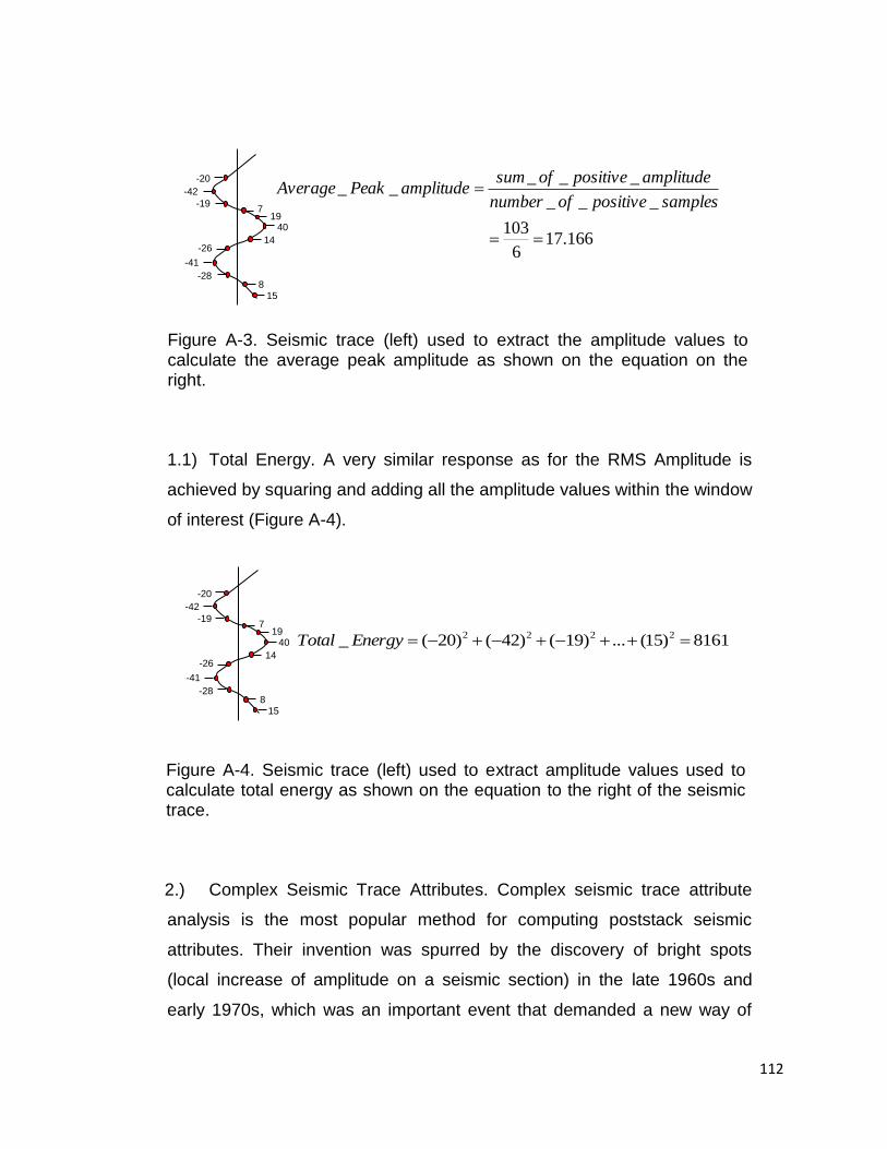
112
1.1) Total Energy. A very similar response as for the RMS Amplitude is
achieved by squaring and adding all the amplitude values within the window
of interest (Figure A-4).
2.) Complex Seismic Trace Attributes. Complex seismic trace attribute
analysis is the most popular method for computing poststack seismic
attributes. Their invention was spurred by the discovery of bright spots
(local increase of amplitude on a seismic section) in the late 1960s and
early 1970s, which was an important event that demanded a new way of
-20
-41
-19
-42
-26
-28
719
40
14
815
166.176
103
___
_____
samplespositiveofnumber
amplitudepositiveofsumamplitudePeakAverage
Figure A-3. Seismic trace (left) used to extract the amplitude values to calculate the average peak amplitude as shown on the equation on the right.
-20
-41
-19
-42
-26
-28
719
40
14
815
8161)15(...)19()42()20(_ 2222 EnergyTotal
Figure A-4. Seismic trace (left) used to extract amplitude values used to calculate total energy as shown on the equation to the right of the seismic trace.
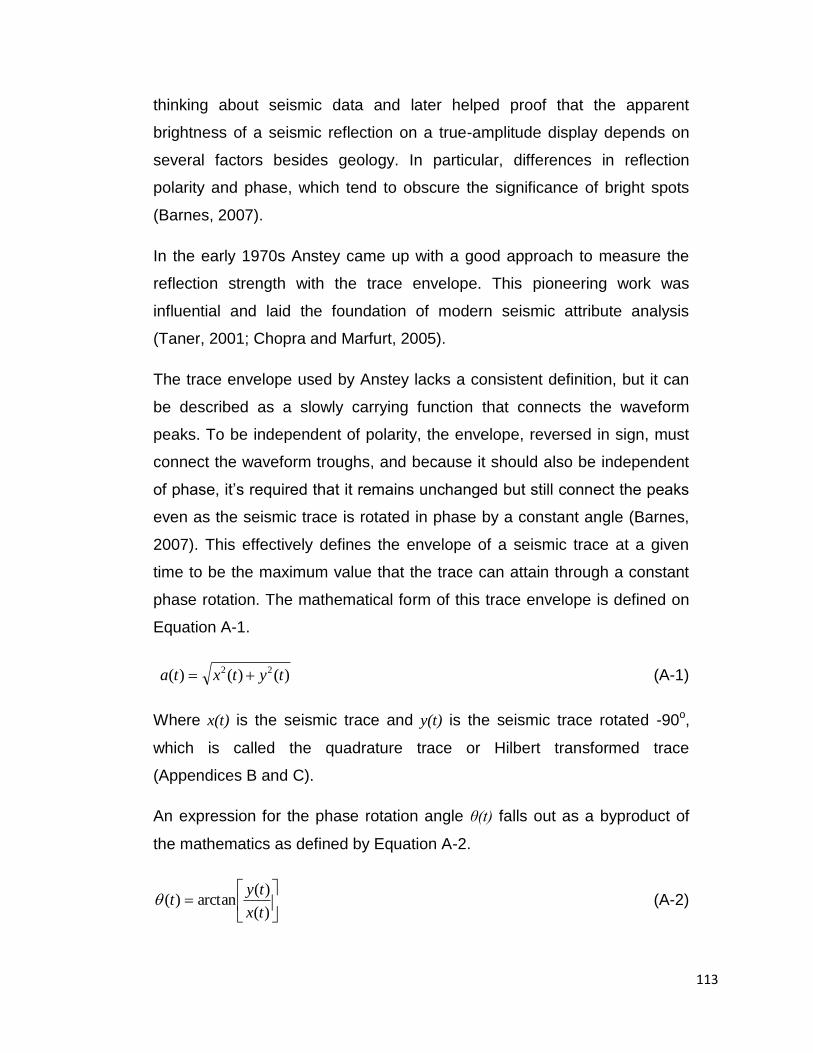
113
thinking about seismic data and later helped proof that the apparent
brightness of a seismic reflection on a true-amplitude display depends on
several factors besides geology. In particular, differences in reflection
polarity and phase, which tend to obscure the significance of bright spots
(Barnes, 2007).
In the early 1970s Anstey came up with a good approach to measure the
reflection strength with the trace envelope. This pioneering work was
influential and laid the foundation of modern seismic attribute analysis
(Taner, 2001; Chopra and Marfurt, 2005).
The trace envelope used by Anstey lacks a consistent definition, but it can
be described as a slowly carrying function that connects the waveform
peaks. To be independent of polarity, the envelope, reversed in sign, must
connect the waveform troughs, and because it should also be independent
of phase, it‟s required that it remains unchanged but still connect the peaks
even as the seismic trace is rotated in phase by a constant angle (Barnes,
2007). This effectively defines the envelope of a seismic trace at a given
time to be the maximum value that the trace can attain through a constant
phase rotation. The mathematical form of this trace envelope is defined on
Equation A-1.
)()()( 22 tytxta (A-1)
Where x(t) is the seismic trace and y(t) is the seismic trace rotated -90o,
which is called the quadrature trace or Hilbert transformed trace
(Appendices B and C).
An expression for the phase rotation angle θ(t) falls out as a byproduct of
the mathematics as defined by Equation A-2.
)(
)(arctan)(
tx
tyt (A-2)
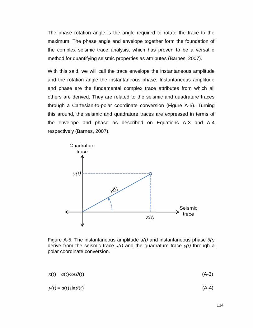
114
The phase rotation angle is the angle required to rotate the trace to the
maximum. The phase angle and envelope together form the foundation of
the complex seismic trace analysis, which has proven to be a versatile
method for quantifying seismic properties as attributes (Barnes, 2007).
With this said, we will call the trace envelope the instantaneous amplitude
and the rotation angle the instantaneous phase. Instantaneous amplitude
and phase are the fundamental complex trace attributes from which all
others are derived. They are related to the seismic and quadrature traces
through a Cartesian-to-polar coordinate conversion (Figure A-5). Turning
this around, the seismic and quadrature traces are expressed in terms of
the envelope and phase as described on Equations A-3 and A-4
respectively (Barnes, 2007).
Figure A-5. The instantaneous amplitude a(t) and instantaneous phase θ(t) derive from the seismic trace x(t) and the quadrature trace y(t) through a polar coordinate conversion.
)(cos)()( ttatx (A-3)
)(sin)()( ttaty (A-4)

115
Thus, a seismic trace can be represented as the product of two
independent and separable functions, instantaneous amplitude and cosine
of the instantaneous phase. This is the essence of complex seismic trace
analysis – separating the amplitude information from the phase information
in the seismic data (Barnes, 2007).
In summary, three main complex attributes can be derived, and these are
described below:
2.1) Reflection Strength (instantaneous envelope or amplitude envelope).
This attribute is calculated as the square root of the total energy of the
seismic signal at an instant (equation A-1) and it is defined as the total
energy of the seismic trace (Taner et al. 1977).
Reflection strength can be thought as amplitude independent of phase with
its values always being greater than or equal to zero (Taner et al. 1977).
This attribute is very sensitive to changes in acoustic impedance and thus
to lithology, porosity, hydrocarbon content from layer to layer. For example,
lateral changes in its values will often be associated with major lithological
changes or with hydrocarbon accumulations, and gas reservoirs in
unconsolidated sands will normally appear as high amplitude (bright spot)
reflections (Taner et al. 1977).
Reflection strength is used in many cases to distinguish massive reflector
from thin-bed composites. In the case of unconformities, the attribute will
vary as subcropping bed changes (Taner et al. 1977).
2.1.1) Slope of the reflection strength, a derived attribute from the reflection
strength that uses its output values, then by a least-squares regression
curve it fits the reflection strength values within the window of interest, with
the slope of this curve being the output of the attribute horizon file. If the
values remain fairly constant, the slope is considered to be close to zero, if
the values increase toward the bottom of the interval, the slope will be
116
positive, and in the opposite case the slope will be negative (Partyka et al.
1998).
This attribute is useful for mapping dominant vertical stratigraphic trends,
and in some cases can be a strong tool for defining the lateral locations of
gas and oil zones (Chopra and Marfurt, 2005).
2.2) Instantaneous Phase. This attribute emphasizes spatial
continuity/discontinuity of reflections by providing a way for weak and strong
events to appear with equal strength (Taner et al. 1977). View θ(t) on
Equation A-3 for a mathematical understanding of this attribute.
Instantaneous phase makes strong events clearer and is effective in
highlighting discontinuities, faults, pinch outs, angularities, and bed
interfaces. Seismic sequence boundaries, sedimentary layer patterns and
regions of onlap/offlap patterns often exhibit extra clarity (Partyka et al.
1998). It is a physical attribute normally used as a discriminator for
geometrical shape classification and in phase velocity computation (Taner
et al. 2001).
2.3) Instantaneous Frequency. This attribute is defined as the rate of
change of the instantaneous phase. It is a measure of time dependent mean
frequency and is independent of phase and amplitude (Partyka et al. 1998). This
attribute responds to both wave propagation effects and depositional
characteristics. Hence it is a physical attribute and can be used as an effective
discriminator (Taner et al. 2001) in some cases such as:
Fracture zone indicator, since fractures may appear as lower frequency
zones.
Bed thickness indicator. Higher frequencies indicate sharp interfaces
while lower frequencies are indicative of more massive bedding
geometries.
117
Other important pieces of information that can also be extracted from this
attribute are the locations where instantaneous frequencies jump or exhibit
a negative sign. These sign reversals are caused by closely-arriving
reflected wavelets. This means, that the time derivative of the phase
function will contain the indicator for thin beds in the form of large variations
of instantaneous frequency (Taner et al. 2001)
Furthermore, destructive interference caused by seismic processing
artifacts such as incorrect Normal Move Out (NMO) or statics corrections
(prior to stacking) can artificially reduce the frequency content affecting the
frequency distribution and consequently this attribute interpretation (Partyka
et al. 1998).
3.) Amplitude variation with offset (AVO). In conventional utilization of the
seismic reflection method, we assumed that the seismic signals can be
viewed as a band-limited normal incidence reflection coefficient series with
appropriate traveltime and amplitude variation due to propagation through
an overburden. Ostrander (1984) demonstrated that the reflection
coefficients in gas-saturated sandstones vary in an anomalous way with
increasing offset and showed how to use this behavior as a direct
hydrocarbon indicator. His work constitutes part of the basis of what today
is known as amplitude variation with offset (AVO) analysis (Castagna et al.
1995; Shuey, 1985; Aki and Richards, 1980).
The variation of reflection and transmission coefficients with incident angle
and thus offset is commonly known as offset-dependent reflectivity. The
Zoeppritz equations (Appendix D) describe how seismic waves are
transmitted and reflected at media boundaries by relating amplitudes of P-
waves and S-waves at each side of the interface. In the general case for an
interface between two solids when the incident angle is not zero, four
waves are generated: reflected P-wave and S-wave and transmitted P-
wave and S-wave. The partition of energy among these is found from four
boundary conditions which require continuity of normal and tangential
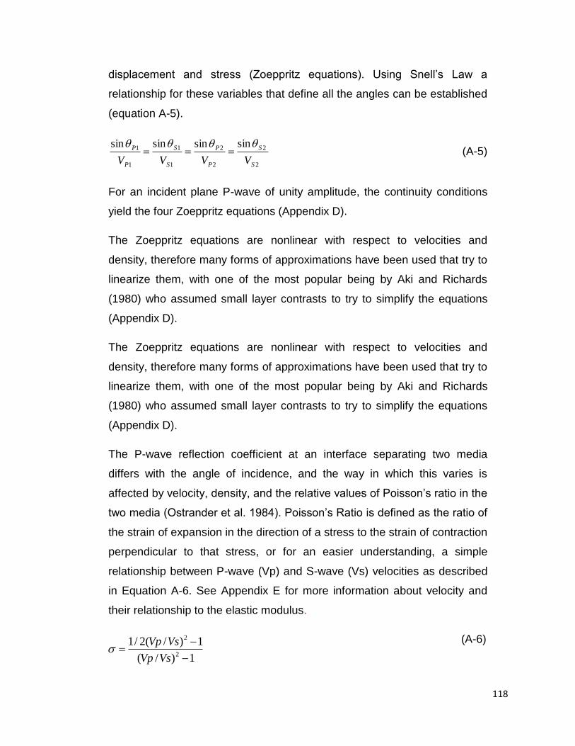
118
1)/(
1)/(2/12
2
VsVp
VsVp
displacement and stress (Zoeppritz equations). Using Snell‟s Law a
relationship for these variables that define all the angles can be established
(equation A-5).
2
2
2
2
1
1
1
1 sinsinsinsin
S
S
P
P
S
S
P
P
VVVV
(A-5)
For an incident plane P-wave of unity amplitude, the continuity conditions
yield the four Zoeppritz equations (Appendix D).
The Zoeppritz equations are nonlinear with respect to velocities and
density, therefore many forms of approximations have been used that try to
linearize them, with one of the most popular being by Aki and Richards
(1980) who assumed small layer contrasts to try to simplify the equations
(Appendix D).
The P-wave reflection coefficient at an interface separating two media
differs with the angle of incidence, and the way in which this varies is
affected by velocity, density, and the relative values of Poisson‟s ratio in the
two media (Ostrander et al. 1984). Poisson‟s Ratio is defined as the ratio of
the strain of expansion in the direction of a stress to the strain of contraction
perpendicular to that stress, or for an easier understanding, a simple
relationship between P-wave (Vp) and S-wave (Vs) velocities as described
in Equation A-6. See Appendix E for more information about velocity and
their relationship to the elastic modulus.
(A-6)
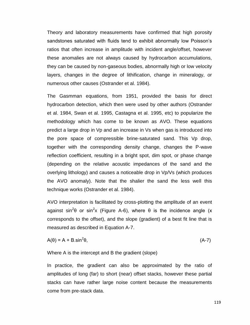
119
Theory and laboratory measurements have confirmed that high porosity
sandstones saturated with fluids tend to exhibit abnormally low Poisson‟s
ratios that often increase in amplitude with incident angle/offset, however
these anomalies are not always caused by hydrocarbon accumulations,
they can be caused by non-gaseous bodies, abnormally high or low velocity
layers, changes in the degree of lithification, change in mineralogy, or
numerous other causes (Ostrander et al. 1984).
The Gasmman equations, from 1951, provided the basis for direct
hydrocarbon detection, which then were used by other authors (Ostrander
et al. 1984, Swan et al. 1995, Castagna et al. 1995, etc) to popularize the
methodology which has come to be known as AVO. These equations
predict a large drop in Vp and an increase in Vs when gas is introduced into
the pore space of compressible brine-saturated sand. This Vp drop,
together with the corresponding density change, changes the P-wave
reflection coefficient, resulting in a bright spot, dim spot, or phase change
(depending on the relative acoustic impedances of the sand and the
overlying lithology) and causes a noticeable drop in Vp/Vs (which produces
the AVO anomaly). Note that the shalier the sand the less well this
technique works (Ostrander et al. 1984).
AVO interpretation is facilitated by cross-plotting the amplitude of an event
against sin2θ or sin2x (Figure A-6), where θ is the incidence angle (x
corresponds to the offset), and the slope (gradient) of a best fit line that is
measured as described in Equation A-7.
A(θ) = A + B.sin2θ, (A-7)
Where A is the intercept and B the gradient (slope)
In practice, the gradient can also be approximated by the ratio of
amplitudes of long (far) to short (near) offset stacks, however these partial
stacks can have rather large noise content because the measurements
come from pre-stack data.

120
By using the plot on Figure 6 three classes of AVO anomalies were initially
proposed by Rutherford and Williams (1982), and a fourth class was later
proposed by Castagna and Swan (1997). Table A-1 summarizes these
classes based on their relative impedance response, their quadrant of
appearance and the amplitude variation with offset.
AVO modeling forms one of the main components of AVO analysis, and
consists of generating pre-stack synthetic gathers using a full elastic wave
equation. The inputs for this task are a P-wave sonic, S-wave sonic, and a
density log, with the results being a pre-stack synthetic seismogram for a
multilayer Earth model.
The analysis to be performed consists of predicting whether there is an
anomalous amplitude response with increasing offset, and if so, what
Figure A-9. Class I to III gas-sands classification done by Rutherford and Williams (1989), based on normal incidence reflection coefficients, with a Class IV gas-sand superimposed proposed by Castagna (1997). The vertical axis is reflection coefficient and the horizontal axis is local angle of incidence. Note that Class III and IV may have identical normal incidence reflection coefficients decreases with increasing angle of incidence while Class III reflection coefficient magnitudes increase.
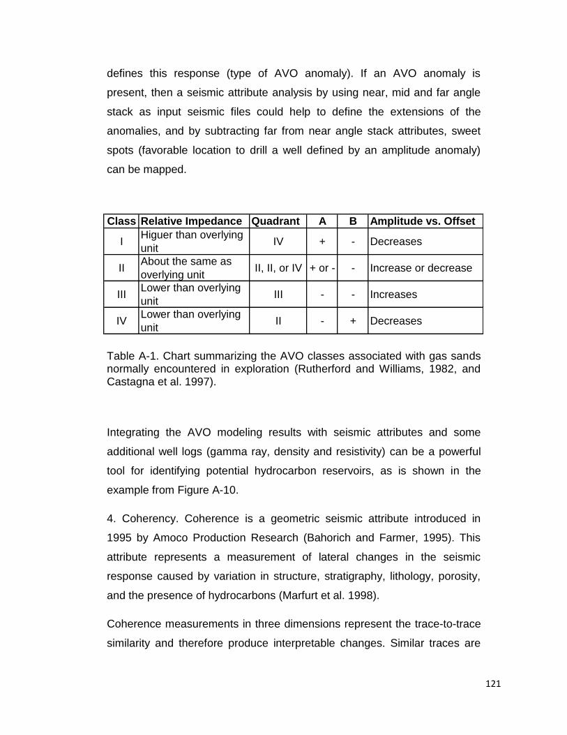
121
Class Relative Impedance Quadrant A B Amplitude vs. Offset
IHiguer than overlying
unitIV + - Decreases
IIAbout the same as
overlying unitII, II, or IV + or - - Increase or decrease
IIILower than overlying
unitIII - - Increases
IVLower than overlying
unitII - + Decreases
defines this response (type of AVO anomaly). If an AVO anomaly is
present, then a seismic attribute analysis by using near, mid and far angle
stack as input seismic files could help to define the extensions of the
anomalies, and by subtracting far from near angle stack attributes, sweet
spots (favorable location to drill a well defined by an amplitude anomaly)
can be mapped.
Table A-1. Chart summarizing the AVO classes associated with gas sands normally encountered in exploration (Rutherford and Williams, 1982, and Castagna et al. 1997).
Integrating the AVO modeling results with seismic attributes and some
additional well logs (gamma ray, density and resistivity) can be a powerful
tool for identifying potential hydrocarbon reservoirs, as is shown in the
example from Figure A-10.
4. Coherency. Coherence is a geometric seismic attribute introduced in
1995 by Amoco Production Research (Bahorich and Farmer, 1995). This
attribute represents a measurement of lateral changes in the seismic
response caused by variation in structure, stratigraphy, lithology, porosity,
and the presence of hydrocarbons (Marfurt et al. 1998).
Coherence measurements in three dimensions represent the trace-to-trace
similarity and therefore produce interpretable changes. Similar traces are
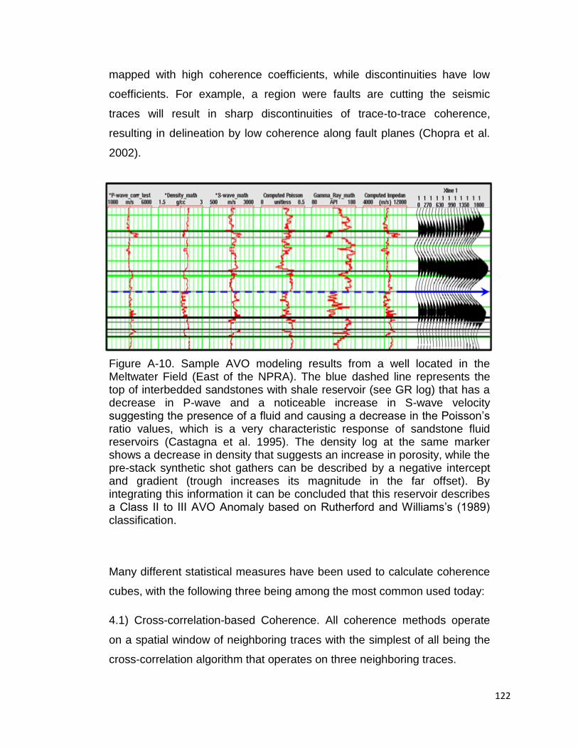
122
mapped with high coherence coefficients, while discontinuities have low
coefficients. For example, a region were faults are cutting the seismic
traces will result in sharp discontinuities of trace-to-trace coherence,
resulting in delineation by low coherence along fault planes (Chopra et al.
2002).
Figure A-10. Sample AVO modeling results from a well located in the Meltwater Field (East of the NPRA). The blue dashed line represents the top of interbedded sandstones with shale reservoir (see GR log) that has a decrease in P-wave and a noticeable increase in S-wave velocity suggesting the presence of a fluid and causing a decrease in the Poisson‟s ratio values, which is a very characteristic response of sandstone fluid reservoirs (Castagna et al. 1995). The density log at the same marker shows a decrease in density that suggests an increase in porosity, while the pre-stack synthetic shot gathers can be described by a negative intercept and gradient (trough increases its magnitude in the far offset). By integrating this information it can be concluded that this reservoir describes a Class II to III AVO Anomaly based on Rutherford and Williams‟s (1989) classification.
Many different statistical measures have been used to calculate coherence
cubes, with the following three being among the most common used today:
4.1) Cross-correlation-based Coherence. All coherence methods operate
on a spatial window of neighboring traces with the simplest of all being the
cross-correlation algorithm that operates on three neighboring traces.
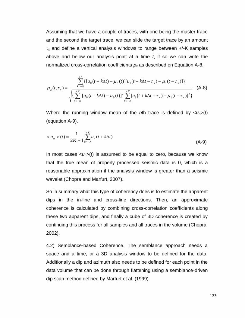
123
Assuming that we have a couple of traces, with one being the master trace
and the second the target trace, we can slide the target trace by an amount
τx and define a vertical analysis windows to range between +/-K samples
above and below our analysis point at a time t, if so we can write the
normalized cross-correlation coefficients ρx as described on Equation A-8.
K
Kk
K
Kk
xx
K
Kk
xxo
xx
ttktuttktu
ttktuttktu
t
})]()([)]()([{
)]}()()][()({[
),(
2
11
2
00
110
(A-8)
Where the running window mean of the nth trace is defined by <un>(t)
(equation A-9).
K
Kk
nn tktuK
tu )(12
1)(
(A-9)
In most cases <un>(t) is assumed to be equal to cero, because we know
that the true mean of properly processed seismic data is 0, which is a
reasonable approximation if the analysis window is greater than a seismic
wavelet (Chopra and Marfurt, 2007).
So in summary what this type of coherency does is to estimate the apparent
dips in the in-line and cross-line directions. Then, an approximate
coherence is calculated by combining cross-correlation coefficients along
these two apparent dips, and finally a cube of 3D coherence is created by
continuing this process for all samples and all traces in the volume (Chopra,
2002).
4.2) Semblance-based Coherence. The semblance approach needs a
space and a time, or a 3D analysis window to be defined for the data.
Additionally a dip and azimuth also needs to be defined for each point in the
data volume that can be done through flattening using a semblance-driven
dip scan method defined by Marfurt et al. (1999).
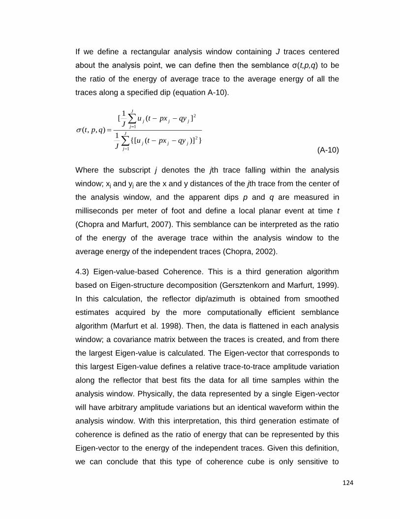
124
If we define a rectangular analysis window containing J traces centered
about the analysis point, we can define then the semblance σ(t,p,q) to be
the ratio of the energy of average trace to the average energy of all the
traces along a specified dip (equation A-10).
J
j
jjj
J
j
jjj
qypxtuJ
qypxtuJ
qpt
1
2
2
1
})]({[1
](1
[
),,(
(A-10)
Where the subscript j denotes the jth trace falling within the analysis
window; xj and yj are the x and y distances of the jth trace from the center of
the analysis window, and the apparent dips p and q are measured in
milliseconds per meter of foot and define a local planar event at time t
(Chopra and Marfurt, 2007). This semblance can be interpreted as the ratio
of the energy of the average trace within the analysis window to the
average energy of the independent traces (Chopra, 2002).
4.3) Eigen-value-based Coherence. This is a third generation algorithm
based on Eigen-structure decomposition (Gersztenkorn and Marfurt, 1999).
In this calculation, the reflector dip/azimuth is obtained from smoothed
estimates acquired by the more computationally efficient semblance
algorithm (Marfurt et al. 1998). Then, the data is flattened in each analysis
window; a covariance matrix between the traces is created, and from there
the largest Eigen-value is calculated. The Eigen-vector that corresponds to
this largest Eigen-value defines a relative trace-to-trace amplitude variation
along the reflector that best fits the data for all time samples within the
analysis window. Physically, the data represented by a single Eigen-vector
will have arbitrary amplitude variations but an identical waveform within the
analysis window. With this interpretation, this third generation estimate of
coherence is defined as the ratio of energy that can be represented by this
Eigen-vector to the energy of the independent traces. Given this definition,
we can conclude that this type of coherence cube is only sensitive to
125
freq
Amp
I
ISweetness
waveform and not to amplitude variations, and will in general provide a
sharper delineation of discontinuities. However, this algorithm degenerates
as the temporal analysis window becomes smaller, when it becomes
increasingly easy to fit all the data in the window with a single spatial
amplitude variation (Chopra, 2002).
6. Sweetness. This seismic attribute was developed by Radovich and
Oliveros (1998) with the goal of identifying shales and sandstones in clastic
successions. Mathematically, it is derived by dividing instantaneous
amplitude (also known as reflection strength or instantaneous envelope) by
the square root of the instantaneous frequency (equation 11). The units for
sweetness are difficult to understand physically, so, this attribute is best
thought as a relative value (Hart, 2008).
(A-11)
Shale-dominated intervals tend to be characterized by low amplitudes
(small acoustic impedance contrasts) and relatively closely spaced
reflections (high frequency), whereas isolated sandy intervals, such as
channel fills and frontal splays, in the shales correspond to high amplitude
(high acoustic impedance contrast with the shales) and low frequency (Hart
et al. 2008).
Parts of the seismic volume described by both high amplitudes and low
frequencies will have high sweetness values; consequently, low amplitudes
with high frequencies will have low sweetness values (Figure A-11).
Sweetness, although a very useful attribute in many cases does not
respond properly when the contrast between sand and shales is low, or if
the destructive interference from reflections above and below the sand
prevent high amplitude reflections from developing (Hart, 2008).
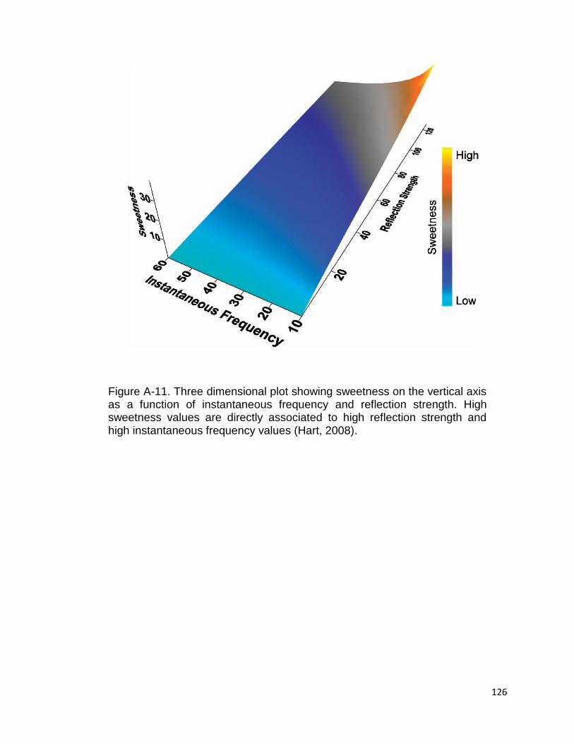
126
Figure A-11. Three dimensional plot showing sweetness on the vertical axis as a function of instantaneous frequency and reflection strength. High sweetness values are directly associated to high reflection strength and high instantaneous frequency values (Hart, 2008).

127
APPENDIX B: Derivation of trace envelope
The trace envelope can be defined as a function that, at any given time, is
the maximum value that a seismic trace can attain through a constant
phase rotation. This definition takes us to a mathematical expression for the
envelope as well as to a formula for the phase rotation angle (Barnes,
2007).
Ideally, a phase rotation changes the phase spectrum by a constant angle
without altering the amplitude spectrum. A phase rotator that subtracts an
angle θ can be expressed as a time-domain convolutional operator p(t,θ)
given by equation B-1.
sin)(cos)(),( thttp (B-1)
Where δ(t) is the delta function and h(t) is the quadrature filter or Hilbert
transform operator (Appendix C). Applying the quadrature filter to a seismic
trace x(t) produces a quadrature trace y(t). Applying the phase subtractor
p(t,θ) to a seismic trace x(t) produces a rotated trace x(t) produces a rotated
x’(t) given as described on equation B-2.
sin)(cos)()(),()(' tytxtxtptx (B-2)
The change of the rotated trace with respect to the rotation angle θ is given
in equation B-3:
cos)(sin)()('
tytxtx
(B-3)
Let θ(t) be the rotation angle that at time t maximizes the value of the
rotated trace. By definition, the envelope a(t) equals this maximum value.
Hence from Equation B-2 we obtain equation B-4:
)(sin)()(cos)()( ttyttxta (B-4)

128
When the rotated trace equals the envelope, its change with respect to
rotation angle θ is zero and θ = θ(t). Hence from equation B-3:
)(cos)()(sin)(0)(
)(ttyttx
t
ta
(B-5)
)(cos)()(sin)( ttyttx (B-6)
An expression for trace envelope follows by squaring equation B-4 and B-5
and adding them to obtain equation B-7.
)()()( 22 tytxta (B-7)
And lastly, an expression for the phase rotation angle is obtained from
equation B-6 as displayed on equation B-8:
)(
)(arctan)(
tx
tyt (B-8)

129
APPENDIX C: Hilbert Transform
The Hilbert transform or quadrature filter is an ideal phase rotator that
subtracts 90o of phase from a seismic trace. Convolving the Hilbert
transform operator h(t) with a cosine wave that has arbitrary amplitude a,
arbitrary but nonzero constant frequency f, and constant phase θ produces
a sine wave of the same amplitude, frequency, and phase, just as
described on equation C-1.
)2sin()2cos()( ftaftath (C-1)
With the constraint of linearity, equation C-1 uniquely defines the Hilbert
transform (Vakman, 1998). Some authors define the Hilbert transform such
that it adds 90o phase, which reverses the sign of the quadrature trace
(e.g., Claerbout, 1985).
The Hilbert transform operator h(t) has the form of equation C-2.
tth
1)( (C-2)
While the Fourier transform H(f), has the form described on equation C-3.
0
)( i
i
fH
0
0
0
f
f
f
(C-3)
The discrete Hilbert transform operator h(n), where n is the sample index is
defined in equation C-4.
0
2
)( nnh 0orevenn
oddn (C-4)
This operator drops off slowly with sample n and so requires long lengths in
application, though half the samples are zero and can be ignored.
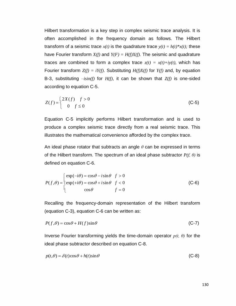
130
Hilbert transformation is a key step in complex seismic trace analysis. It is
often accomplished in the frequency domain as follows. The Hilbert
transform of a seismic trace x(t) is the quadrature trace y(t) = h(t)*x(t); these
have Fourier transform X(f) and Y(F) = H(f)X(f). The seismic and quadrature
traces are combined to form a complex trace z(t) = x(t)+iy(t), which has
Fourier transform Z(f) = iY(f). Substituting H(f)X(f) for Y(f) and, by equation
B-3, substituting –isin(f) for H(f), it can be shown that Z(f) is one-sided
according to equation C-5.
00
0)(2)(
f
ffXfZ (C-5)
Equation C-5 implicitly performs Hilbert transformation and is used to
produce a complex seismic trace directly from a real seismic trace. This
illustrates the mathematical convenience afforded by the complex trace.
An ideal phase rotator that subtracts an angle θ can be expressed in terms
of the Hilbert transform. The spectrum of an ideal phase subtractor P(f, θ) is
defined on equation C-6.
cos
sincos)exp(
sincos)exp(
),( ii
ii
fP
0
0
0
f
f
f
(C-6)
Recalling the frequency-domain representation of the Hilbert transform
(equation C-3), equation C-6 can be written as:
sin)(cos),( fHfP (C-7)
Inverse Fourier transforming yields the time-domain operator p(t, θ) for the
ideal phase subtractor described on equation C-8.
sin)(cos)(),( thttp (C-8)
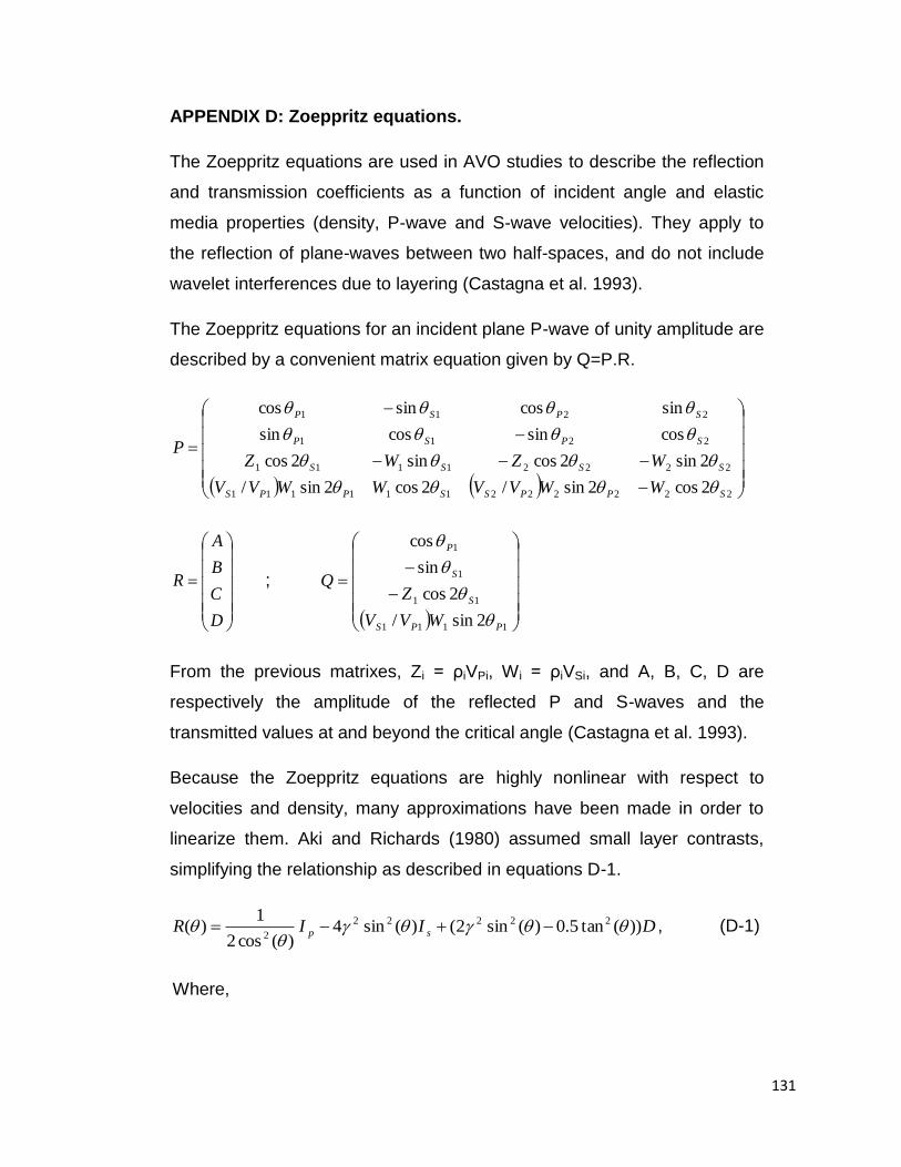
131
APPENDIX D: Zoeppritz equations.
The Zoeppritz equations are used in AVO studies to describe the reflection
and transmission coefficients as a function of incident angle and elastic
media properties (density, P-wave and S-wave velocities). They apply to
the reflection of plane-waves between two half-spaces, and do not include
wavelet interferences due to layering (Castagna et al. 1993).
The Zoeppritz equations for an incident plane P-wave of unity amplitude are
described by a convenient matrix equation given by Q=P.R.
222222111111
22221111
2211
2211
2cos2sin/2cos2sin/
2sin2cossin2cos
cossincossin
sincossincos
SPPSSPPS
SSSS
SPSP
SPSP
WWVVWWVV
WZWZP
D
C
B
A
R ;
1111
11
1
1
2sin/
2cos
sin
cos
PPS
S
S
P
WVV
ZQ
From the previous matrixes, Zi = ρiVPi, Wi = ρiVSi, and A, B, C, D are
respectively the amplitude of the reflected P and S-waves and the
transmitted values at and beyond the critical angle (Castagna et al. 1993).
Because the Zoeppritz equations are highly nonlinear with respect to
velocities and density, many approximations have been made in order to
linearize them. Aki and Richards (1980) assumed small layer contrasts,
simplifying the relationship as described in equations D-1.
DIIR sp ))(tan5.0)(sin2()(sin4)(cos2
1)( 22222
2
, (D-1)
Where,
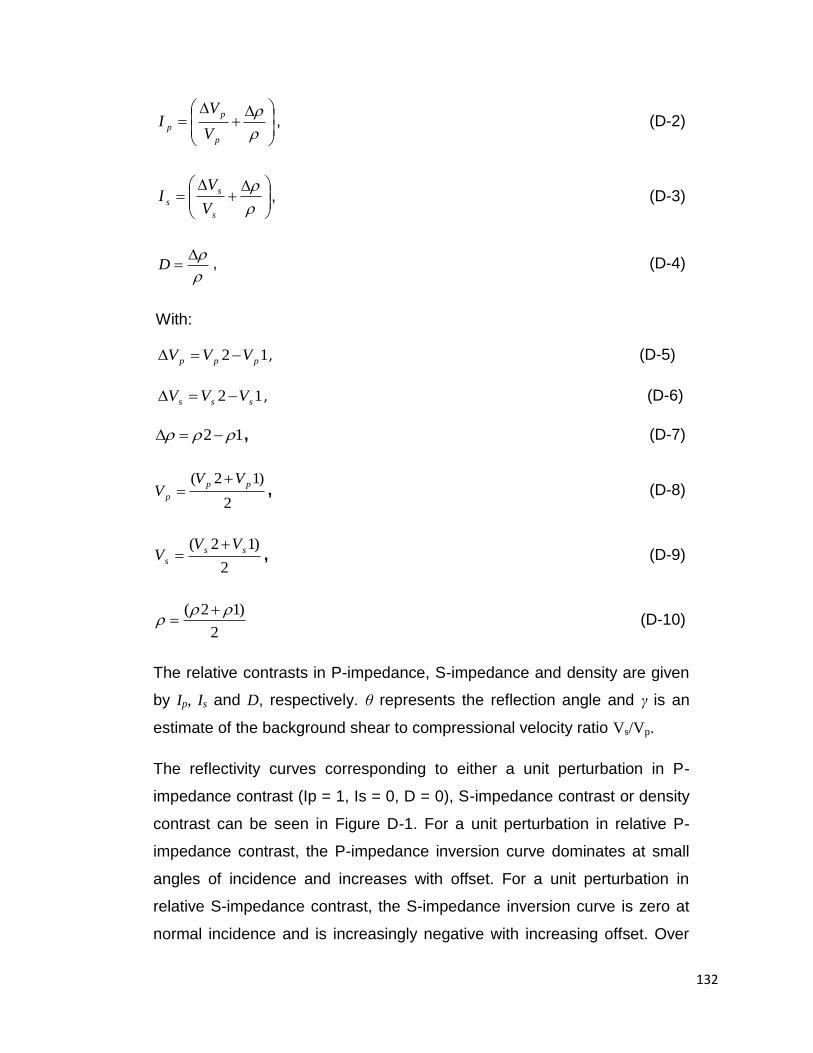
132
p
p
pV
VI , (D-2)
s
s
sV
VI , (D-3)
D , (D-4)
With:
12 ppp VVV , (D-5)
12 sss VVV , (D-6)
12 , (D-7)
2
)12( pp
p
VVV
, (D-8)
2
)12( ss
s
VVV
, (D-9)
2
)12(
(D-10)
The relative contrasts in P-impedance, S-impedance and density are given
by Ip, Is and D, respectively. θ represents the reflection angle and γ is an
estimate of the background shear to compressional velocity ratio Vs/Vp.
The reflectivity curves corresponding to either a unit perturbation in P-
impedance contrast (Ip = 1, Is = 0, D = 0), S-impedance contrast or density
contrast can be seen in Figure D-1. For a unit perturbation in relative P-
impedance contrast, the P-impedance inversion curve dominates at small
angles of incidence and increases with offset. For a unit perturbation in
relative S-impedance contrast, the S-impedance inversion curve is zero at
normal incidence and is increasingly negative with increasing offset. Over
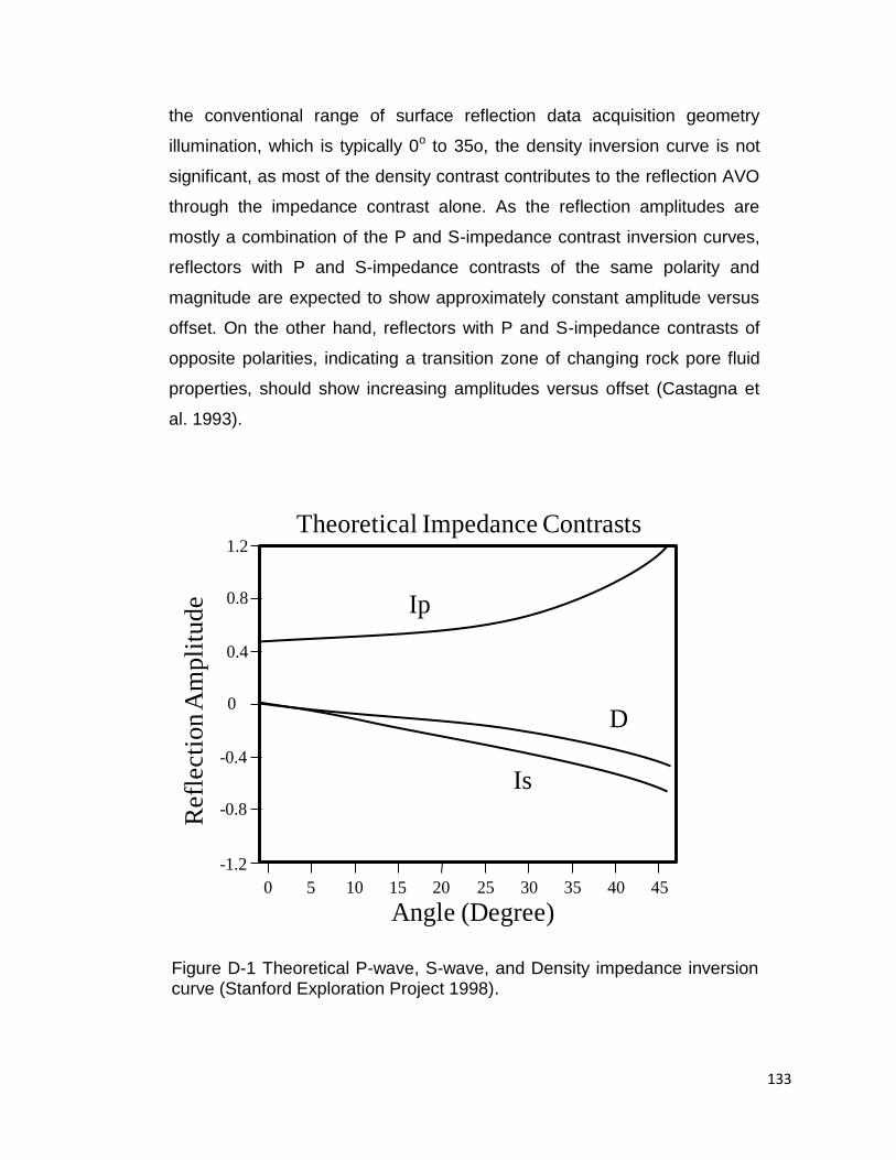
133
the conventional range of surface reflection data acquisition geometry
illumination, which is typically 0o to 35o, the density inversion curve is not
significant, as most of the density contrast contributes to the reflection AVO
through the impedance contrast alone. As the reflection amplitudes are
mostly a combination of the P and S-impedance contrast inversion curves,
reflectors with P and S-impedance contrasts of the same polarity and
magnitude are expected to show approximately constant amplitude versus
offset. On the other hand, reflectors with P and S-impedance contrasts of
opposite polarities, indicating a transition zone of changing rock pore fluid
properties, should show increasing amplitudes versus offset (Castagna et
al. 1993).
Theoretical Impedance Contrasts
Angle (Degree)
Refl
ecti
on A
mpli
tude
0 5 10 15 20 25 30 35 40 45
-1.2
-0.8
-0.4
0
0.4
0.8
1.2
Ip
D
Is
Figure D-1 Theoretical P-wave, S-wave, and Density impedance inversion curve (Stanford Exploration Project 1998).
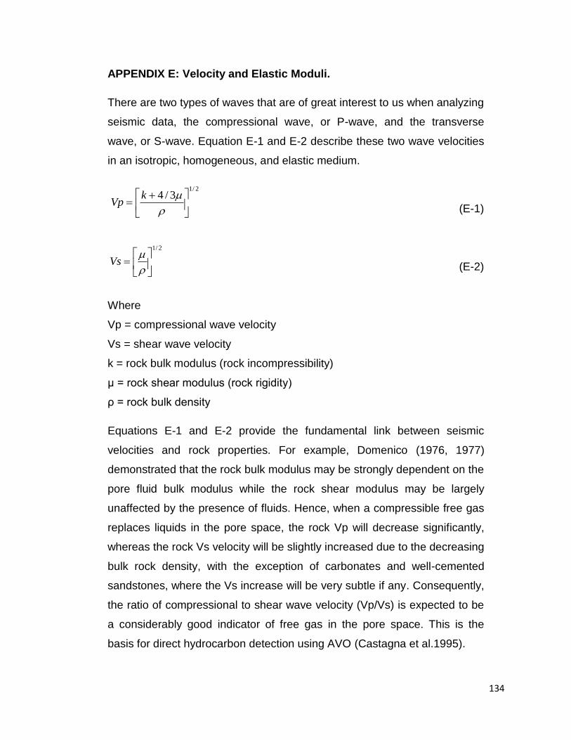
134
2/1
3/4
kVp
2/1
Vs
APPENDIX E: Velocity and Elastic Moduli.
There are two types of waves that are of great interest to us when analyzing
seismic data, the compressional wave, or P-wave, and the transverse
wave, or S-wave. Equation E-1 and E-2 describe these two wave velocities
in an isotropic, homogeneous, and elastic medium.
(E-1)
(E-2)
Where
Vp = compressional wave velocity
Vs = shear wave velocity
k = rock bulk modulus (rock incompressibility)
μ = rock shear modulus (rock rigidity)
ρ = rock bulk density
Equations E-1 and E-2 provide the fundamental link between seismic
velocities and rock properties. For example, Domenico (1976, 1977)
demonstrated that the rock bulk modulus may be strongly dependent on the
pore fluid bulk modulus while the rock shear modulus may be largely
unaffected by the presence of fluids. Hence, when a compressible free gas
replaces liquids in the pore space, the rock Vp will decrease significantly,
whereas the rock Vs velocity will be slightly increased due to the decreasing
bulk rock density, with the exception of carbonates and well-cemented
sandstones, where the Vs increase will be very subtle if any. Consequently,
the ratio of compressional to shear wave velocity (Vp/Vs) is expected to be
a considerably good indicator of free gas in the pore space. This is the
basis for direct hydrocarbon detection using AVO (Castagna et al.1995).
135
For a homogeneous isotropic material which is deforming elastically under
uniaxial compression, Poisson‟s ratio (σ) is defined as the negative
fractional change in length. Poisson‟s ratio is directly related to the Vp/Vs
ratio by equation E-3.
1)/(
1)/(5.0
2
2
sp
sp
VV
VV (E-3)
A Poisson‟s ratio equal to zero corresponds to Vp/Vs equal to 1.41. Fluids
have a Poisson‟s ratio of 0.5, where Vp/Vs equals infinity.
The shear modulus (μ) is the ratio of shear stress to shear strain. Similarly,
the bulk modulus (k) is the ratio of volumetric stress to volumetric strain and
is the reciprocal of the compressibility (Castagna et al. 1995).
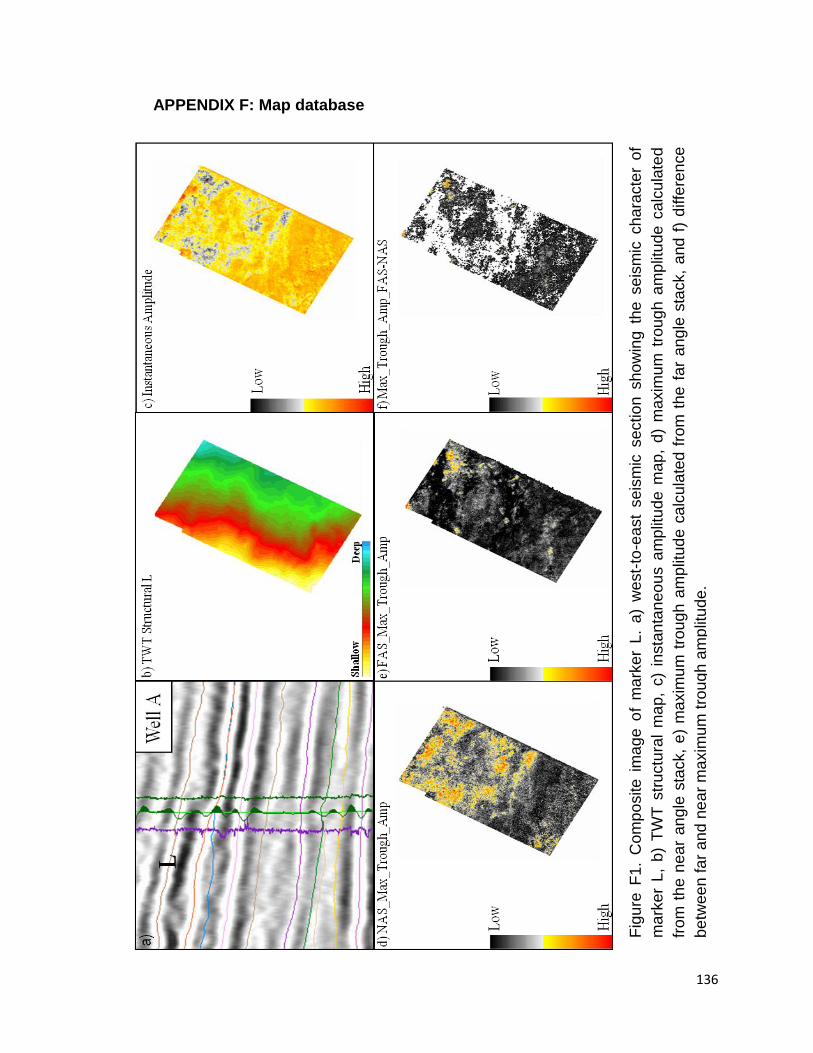
136
APPENDIX F: Map database
Fig
ure
F1.
Com
po
site i
ma
ge
of
ma
rker
L.
a)
west-
to-e
ast
se
ism
ic s
ectio
n s
ho
win
g t
he s
eis
mic
ch
ara
cte
r o
f
ma
rker
L,
b)
TW
T s
tru
ctu
ral
ma
p,
c)
insta
nta
neo
us a
mp
litu
de m
ap
, d
) m
axim
um
tro
ug
h a
mp
litu
de
ca
lcula
ted
from
th
e n
ea
r an
gle
sta
ck,
e)
ma
xim
um
tro
ug
h a
mp
litud
e c
alc
ula
ted
fro
m t
he
fa
r an
gle
sta
ck,
and
f)
diffe
ren
ce
be
twee
n fa
r and
ne
ar
ma
xim
um
tro
ug
h a
mp
litu
de.
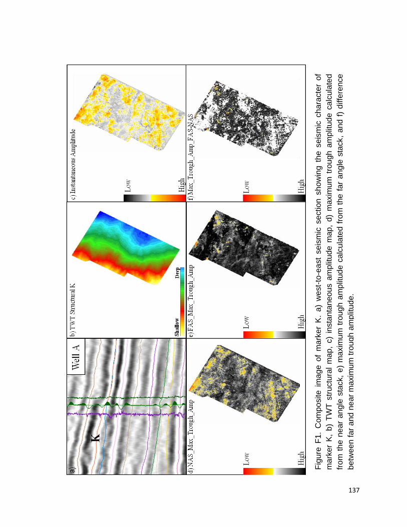
137
Fig
ure
F1.
Com
po
site i
ma
ge
of
ma
rker
K.
a)
west-
to-e
ast
se
ism
ic s
ectio
n s
ho
win
g t
he s
eis
mic
ch
ara
cte
r o
f
ma
rker
K,
b)
TW
T s
tructu
ral
ma
p,
c)
insta
nta
neo
us a
mp
litud
e m
ap
, d
) m
axim
um
tro
ugh a
mp
litu
de
ca
lcula
ted
from
th
e n
ea
r an
gle
sta
ck,
e)
ma
xim
um
tro
ug
h a
mp
litud
e c
alc
ula
ted
fro
m t
he
fa
r an
gle
sta
ck,
and
f)
diffe
ren
ce
be
twee
n fa
r and
ne
ar
ma
xim
um
tro
ug
h a
mp
litu
de.
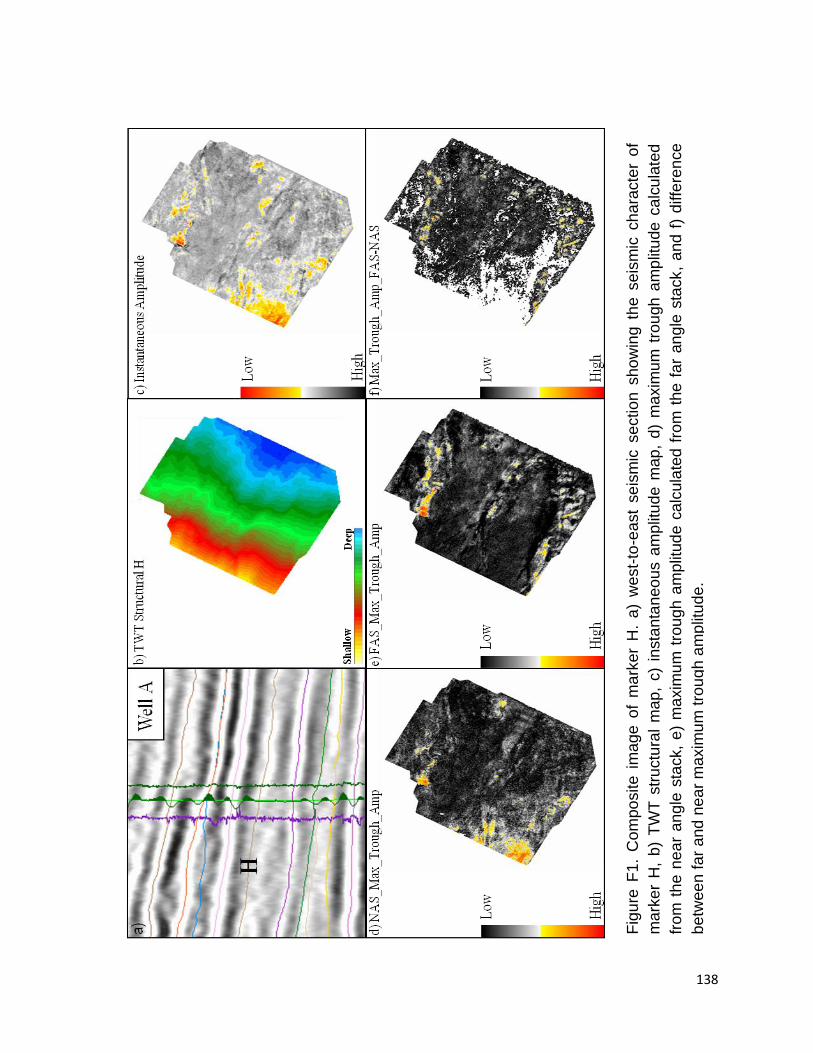
138
Fig
ure
F1.
Com
po
site i
ma
ge
of
ma
rker
H.
a)
west-
to-e
ast
se
ism
ic s
ectio
n s
ho
win
g t
he s
eis
mic
ch
ara
cte
r o
f
ma
rker
H,
b)
TW
T s
tru
ctu
ral
map
, c)
insta
nta
neo
us a
mp
litu
de
map
, d
) m
axim
um
tro
ugh a
mp
litu
de
ca
lcu
late
d
from
th
e n
ea
r an
gle
sta
ck,
e)
ma
xim
um
tro
ug
h a
mp
litud
e c
alc
ula
ted
fro
m t
he
fa
r an
gle
sta
ck,
and
f)
diffe
ren
ce
be
twee
n fa
r and
ne
ar
ma
xim
um
tro
ug
h a
mp
litu
de.
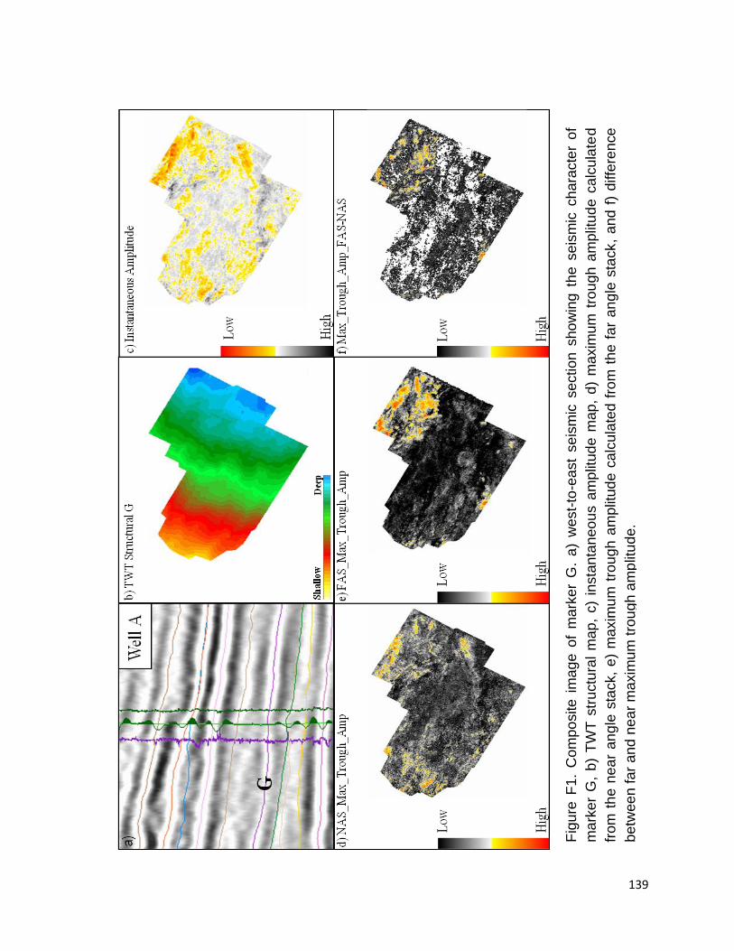
139
Fig
ure
F1.
Com
po
site i
ma
ge
of
ma
rker
G.
a)
west-
to-e
ast
se
ism
ic s
ectio
n s
ho
win
g t
he s
eis
mic
ch
ara
cte
r o
f
ma
rker
G,
b)
TW
T s
tru
ctu
ral
ma
p,
c)
insta
nta
neo
us a
mp
litud
e m
ap
, d
) m
axim
um
tro
ug
h a
mp
litu
de
ca
lcula
ted
from
th
e n
ea
r an
gle
sta
ck,
e)
ma
xim
um
tro
ug
h a
mp
litud
e c
alc
ula
ted
fro
m t
he
fa
r an
gle
sta
ck,
and
f)
diffe
ren
ce
be
twee
n fa
r and
ne
ar
ma
xim
um
tro
ug
h a
mp
litu
de.
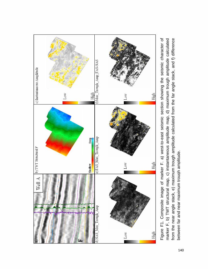
140
Fig
ure
F1.
Co
mp
osite i
ma
ge
of
ma
rker
F.
a)
west-
to-e
ast
se
ism
ic s
ectio
n s
ho
win
g t
he s
eis
mic
ch
ara
cte
r of
ma
rker
F,
b)
TW
T s
tru
ctu
ral
ma
p,
c)
insta
nta
neo
us a
mp
litu
de
ma
p,
d)
ma
xim
um
tro
ug
h a
mp
litu
de
ca
lcula
ted
from
th
e n
ea
r an
gle
sta
ck,
e)
ma
xim
um
tro
ug
h a
mp
litud
e c
alc
ula
ted
fro
m t
he
fa
r an
gle
sta
ck,
and
f)
diffe
ren
ce
be
twee
n fa
r and
ne
ar
ma
xim
um
tro
ug
h a
mp
litu
de.
141
Fig
ure
F1.
Com
po
site
im
ag
e o
f m
ark
er
E_
a.
a)
west-
to-e
ast
se
ism
ic s
ectio
n s
ho
win
g t
he
se
ism
ic c
ha
racte
r of
ma
rker
E_
a b
) T
WT
str
uctu
ral
ma
p,
c)
insta
nta
neo
us a
mp
litu
de
map
, d
) m
axim
um
tro
ugh a
mp
litu
de
ca
lcula
ted
from
th
e n
ea
r an
gle
sta
ck,
e)
ma
xim
um
tro
ug
h a
mp
litud
e c
alc
ula
ted
fro
m t
he
fa
r an
gle
sta
ck,
and
f)
diffe
ren
ce
be
twee
n fa
r and
ne
ar
ma
xim
um
tro
ug
h a
mp
litu
de.
142
Fig
ure
F1.
Com
po
site i
ma
ge
of
ma
rker
E.
a)
west-
to-e
ast
se
ism
ic s
ectio
n s
ho
win
g t
he s
eis
mic
ch
ara
cte
r o
f
ma
rker
E,
b)
TW
T s
tructu
ral
ma
p,
c)
insta
nta
neo
us a
mp
litud
e m
ap
, d
) m
axim
um
tro
ugh a
mp
litu
de
ca
lcula
ted
from
th
e n
ea
r an
gle
sta
ck,
e)
ma
xim
um
tro
ug
h a
mp
litud
e c
alc
ula
ted
fro
m t
he
fa
r an
gle
sta
ck,
and
f)
diffe
ren
ce
be
twee
n fa
r and
ne
ar
ma
xim
um
tro
ug
h a
mp
litu
de.

143
Fig
ure
F1.
Com
po
site i
ma
ge
of
ma
rker
D.
a)
west-
to-e
ast
se
ism
ic s
ectio
n s
ho
win
g t
he s
eis
mic
ch
ara
cte
r o
f
ma
rker
D,
b)
TW
T s
tru
ctu
ral
map
, c)
insta
nta
neo
us a
mp
litu
de
map
, d
) m
axim
um
tro
ugh a
mp
litu
de
ca
lcu
late
d
from
th
e n
ea
r an
gle
sta
ck,
e)
ma
xim
um
tro
ug
h a
mp
litud
e c
alc
ula
ted
fro
m t
he
fa
r an
gle
sta
ck,
and
f)
diffe
ren
ce
be
twee
n fa
r and
ne
ar
ma
xim
um
tro
ug
h a
mp
litu
de.
144
Fig
ure
F1.
Com
po
site i
ma
ge
of
ma
rker
Ca
. a
) w
est-
to-e
ast
se
ism
ic s
ectio
n s
ho
win
g t
he s
eis
mic
ch
ara
cte
r o
f
ma
rker
Ca
, b
) T
WT
str
uctu
ral
ma
p,
c)
insta
nta
neo
us a
mp
litu
de
map
, d
) m
axim
um
tro
ugh a
mp
litu
de
ca
lcu
late
d
from
th
e n
ea
r an
gle
sta
ck,
e)
ma
xim
um
tro
ug
h a
mp
litud
e c
alc
ula
ted
fro
m t
he
fa
r an
gle
sta
ck,
and
f)
diffe
ren
ce
be
twee
n fa
r and
ne
ar
ma
xim
um
tro
ug
h a
mp
litu
de.
145
Fig
ure
F1.
Com
po
site i
ma
ge
of
ma
rker
B.
a)
west-
to-e
ast
se
ism
ic s
ectio
n s
ho
win
g t
he s
eis
mic
ch
ara
cte
r o
f
ma
rker
B,
b)
TW
T s
tructu
ral
ma
p,
c)
insta
nta
neo
us a
mp
litud
e m
ap
, d
) m
axim
um
tro
ugh a
mp
litu
de
ca
lcula
ted
from
th
e n
ea
r an
gle
sta
ck,
e)
ma
xim
um
tro
ug
h a
mp
litud
e c
alc
ula
ted
fro
m t
he
fa
r an
gle
sta
ck,
and
f)
diffe
ren
ce
be
twee
n fa
r and
ne
ar
ma
xim
um
tro
ug
h a
mp
litu
de.
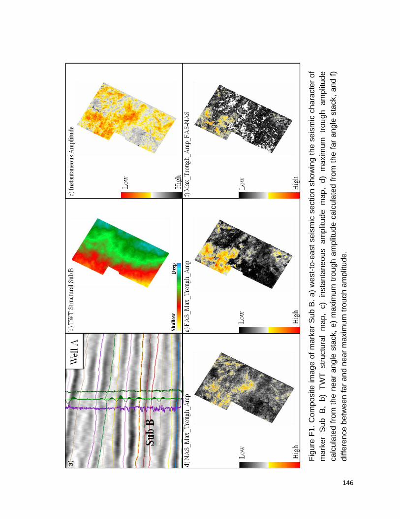
146
Fig
ure
F1.
Com
po
site
im
ag
e o
f m
ark
er
Sub
B.
a)
west-
to-e
ast
se
ism
ic s
ectio
n s
ho
win
g t
he s
eis
mic
ch
ara
cte
r o
f
ma
rker
Su
b
B,
b)
TW
T
str
uctu
ral
ma
p,
c)
insta
nta
ne
ou
s
am
plit
ud
e
ma
p,
d)
ma
xim
um
tr
ou
gh
a
mp
litude
ca
lcula
ted
fro
m t
he
nea
r a
ng
le s
tack,
e)
ma
xim
um
tro
ug
h a
mp
litu
de
ca
lcula
ted
fro
m t
he
fa
r a
ng
le s
tack,
and
f)
diffe
ren
ce
be
twee
n fa
r a
nd
ne
ar
ma
xim
um
tro
ug
h a
mp
litu
de
.
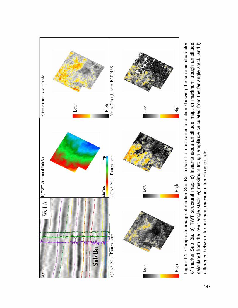
147
Fig
ure
F1.
Com
po
site
im
ag
e o
f m
ark
er
Su
b B
a.
a)
west-
to-e
ast
se
ism
ic s
ectio
n s
ho
win
g t
he
se
ism
ic c
ha
racte
r
of
ma
rker
Su
b B
a,
b)
TW
T s
tructu
ral
ma
p,
c)
insta
nta
ne
ou
s a
mp
litu
de
ma
p,
d)
ma
xim
um
tro
ug
h a
mp
litude
ca
lcula
ted
fro
m t
he
nea
r a
ng
le s
tack,
e)
ma
xim
um
tro
ug
h a
mp
litu
de
ca
lcula
ted
fro
m t
he
fa
r a
ng
le s
tack,
and
f)
diffe
ren
ce
be
twee
n fa
r a
nd
ne
ar
ma
xim
um
tro
ug
h a
mp
litu
de
.
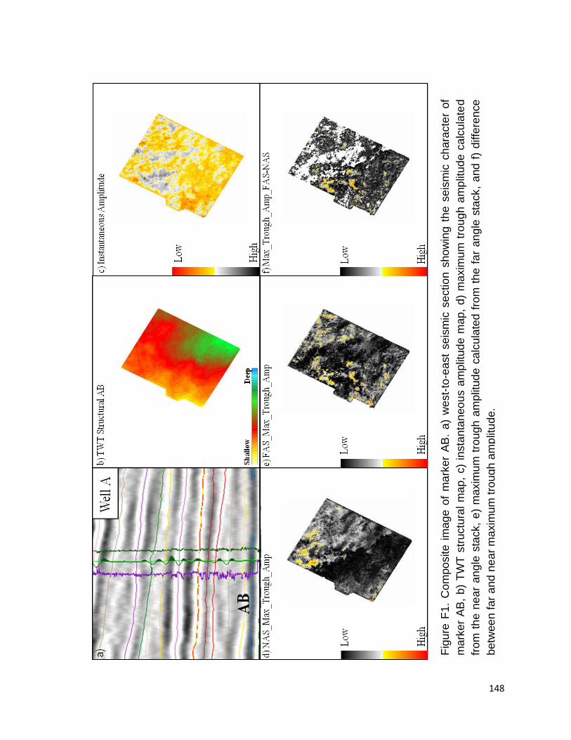
148
Fig
ure
F1.
Com
po
site i
ma
ge
of
ma
rker
AB
. a
) w
est-
to-e
ast
se
ism
ic s
ectio
n s
ho
win
g t
he s
eis
mic
ch
ara
cte
r of
ma
rker
AB
, b
) T
WT
str
uctu
ral
ma
p,
c)
insta
nta
neo
us a
mp
litud
e m
ap
, d
) m
axim
um
tro
ug
h a
mp
litu
de
ca
lcula
ted
from
th
e n
ea
r an
gle
sta
ck,
e)
ma
xim
um
tro
ug
h a
mp
litud
e c
alc
ula
ted
fro
m t
he
fa
r an
gle
sta
ck,
and
f)
diffe
ren
ce
be
twee
n fa
r and
ne
ar
ma
xim
um
tro
ug
h a
mp
litu
de.
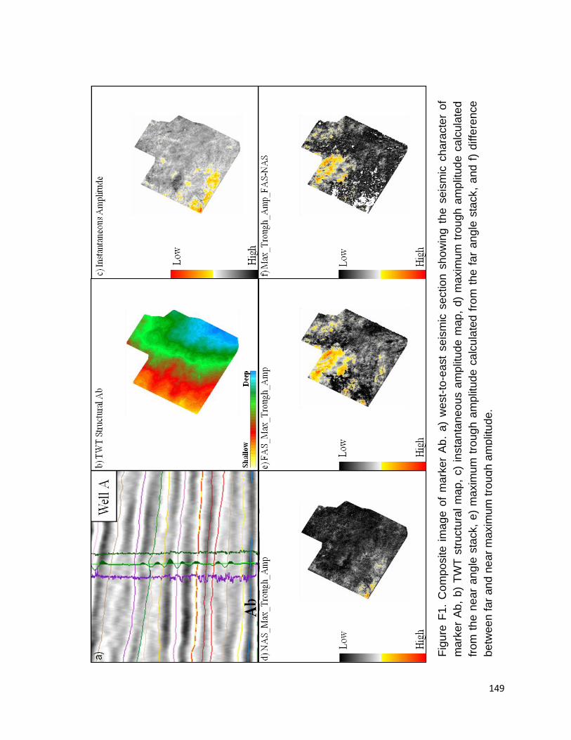
149
Fig
ure
F1.
Com
po
site i
ma
ge
of
ma
rker
Ab
. a
) w
est-
to-e
ast
se
ism
ic s
ectio
n s
ho
win
g t
he s
eis
mic
ch
ara
cte
r o
f
ma
rker
Ab
, b
) T
WT
str
uctu
ral
ma
p,
c)
insta
nta
neo
us a
mp
litud
e m
ap
, d
) m
axim
um
tro
ugh a
mp
litu
de
ca
lcula
ted
from
th
e n
ea
r an
gle
sta
ck,
e)
ma
xim
um
tro
ug
h a
mp
litud
e c
alc
ula
ted
fro
m t
he
fa
r an
gle
sta
ck,
and
f)
diffe
ren
ce
be
twee
n fa
r and
ne
ar
ma
xim
um
tro
ug
h a
mp
litu
de.


![TAR-SANDS (ARENAS BITUMINOSAS) [OIL-SANDS]](https://img.pdfslide.net/doc/110x75/546e6d60b4af9faa268b468b/tar-sands-arenas-bituminosas-oil-sands.jpg)