Identification of rotating sound source based on

22ème Congrès Français de Mécanique Lyon, 24 au 28 Août 2015

Identification of rotating sound source based on microphone array measurements

L. GENGa,b, Q. LECLEREb, A. PEREIRAb,c, C.X. BIa

a. Institute of Sound and Vibration Research, Hefei University of Technology, 193 Tunxi

Road, Hefei 230009, People’s Republic of China, [email protected] b. Laboratoire Vibrations Acoustique, INSA Lyon, 25 bis av. J. Capelle 69621 Villeurbanne

cedex, [email protected] c. Laboratoire de Mécanique des Fluides et d’Acoustique, École Centrale de Lyon, 36, avenue

Guy de Collongue, 69134 Écully cedex

Abstract:

A time-domain beamforming method based on microphone array measurements is applied to identify the location of the rotating sound source. The identification process of the beamforming method is briefly described first. And then, numerical simulations of two rotating monopole sources generating different signals at a constant angular frequency are investigated to testify the feasibility of the time-domain beamforming method. The simulation results demonstrate that this beamforming method can identify the locations of these two rotating sources very well. Finally, an experiment of a rotating disk with two small speakers is carried out to further show the identification ability of the beamforming method. The experimental results demonstrate that this beamforming method is effective in identifying the location of rotating source.

1 Introduction Microphone array measurements have become a standard technique to localize and quantify

source in kinds of sound fields. The simplest approach is the beamforming that applies the phase differences between the measured signals to determine the direction of arrival of the wave fronts and provides the beamform map for the locations of the source, which constitutes the delay and sum (DS) beamforming method. These possible source positions on the focus surface can be identified by adjusting the delay times of the microphone signals relative to each other, and the strengths of the investigated sources can be shown in the beamform map. Microphone array measurements are expanded to locate the moving source [1-2]. A dedopplerization technique [3] is introduced to place the moving source into a moving reference frame. Here, the rotating source with a constant angular frequency is focused. The DS beamforming method is extended for the rotating source, which is called Rotating Source Identifier (ROSI) beamforming method [4]. The calculation is performed in the time domain. Besides, the Rotating Beamforming method [5] in the frequency domain is also useful for investigating the rotating source. The purpose of this paper is to display the identification ability of ROSI beamforming. The identification process of this method is briefly recalled first. Numerical simulations of two rotating monopole sources driven by different signals are used to testify the ROSI beamforming method. And then, this method is experimentally applied to identify the locations of two small speakers installed in a rotating disk in a semi-anechoic chamber.


2 Theory of ROSI beamforming The general solution ),( trp in the wave equation for a rotating monopole source can be

expressed as [4]

),(4),(

),(τπ

τwR

rstrp s= , (1)

where ),( τsrs is the rotating source signal, sr is the time-dependent position of the rotating source,

w is the angular frequency of the rotation, z-axis is the rotating axis, srrwR −=),( τ is the distance

between the field point r and the rotating source, and the emission time τ is a solution of the following equation:

),()( ττ wRtc =− , (2)

where c is the sound velocity.

Figure 1. Geometric description of the measurement plane H, the focusing plane E, and the rotating monopole source.

Figure 1 shows the geometry of the measurement plane H, the focusing plane E, and the rotating monopole source. There are M measurement points distributed on the plane H and N focusing points

distributed on the plane E. Suppose ),( trpm (m=1,…,M) are the pressure signal recorded by M

microphones. If a virtual point source located at er on the focusing plane E is present, the microphone

pressure signal ),( trpm can be written as

),(4),(

),(e

eem wR

rstrp

τπτ= . (3)

In order to reconstruct the virtual source signal ),( eers τ from the pressure signal ),( trpm , the

emission time is fixed. The Eq. (3) can be rewritten as

),(4),(

),(e

eeim wR

rstrp

τπτ= . (4)

The receiver time it of the microphone can be calculated by,

cwRt eei /),( ττ += . (5)

The reconstructed signal ),(~eers τ can be calculated with the delay and sum procedure:

),(),(~1

im

M

mmee trpwrs ∑

=

=τ , (6)

where mw is the beamforming steering vector.


3 Numerical simulation Numerical simulation with two rotating monopole sources is investigated to testify the feasibility

of the ROSI beamforming method. The geometry of two rotating sources, the measurement ring H and the focusing plane E are shown in Fig. 2. The initial locations of the rotating monopole sources S1 and S2 are (0.15 m, 0 m, 0 m) and (0 m, 0.1 m, 0 m) , respectively. The measurement ring H is located at

z=0.15 m in the Cartesian coordinate system ),,( zyxo . The measurement ring H provides 50

measured points. The focusing plane E with 13× 13 points is located at =z 0 m and the grid spacing is 0.05 m in both x and y directions. The rotating frequency is set as 50 Hz. The pressure signal is simulated with a sampling frequency of 25.6 kHz, providing 5120 sampling points. The theoretical pressure generated by the rotating monopole source is calculated according to the advance time approach in Ref. [6].

Figure 2. Geometry of two rotating monopole sources, the measurement ring H, and the focusing plane

E in the Cartesian coordinate system ),,( zyxo .

3.1 Sweep frequency signal The rotating sources S1 and S2 generate sweep frequency signals in the [2000, 6000] Hz band. A

Gaussian white noise with a signal-to-noise ratio of 20 dB is added to the simulated signals. The time-domain pressure waveform at one microphone without rotation is shown in Fig. 3(a),

and its spectrum is depicted in Fig. 3(b), which contains contributions of two correlated sources during the sweep. The time-domain pressure waveform at the microphone with rotation and its spectrum are shown in Figs. 3(c) and 3(d), respectively. In Fig. 3, it can be found that the pressure signals generated by rotating monopole source are different from those without rotation. The ROSI beamforming method is applied to the rotating data. The identification maps at two 1/3 octave frequencies are shown in Fig. 4. It is obvious that the two rotating monopole sources are identified very well.


Figure 3. (a) Pressure signal at one microphone without rotation and (b) its spectrum signal, and (c) pressure signal at one microphone with rotation and (d) its spectrum signal.

Figure 4. Identification maps at 1/3 octave (a) 2000 Hz, and (b) 4000 Hz. The rotating frequency is 50 Hz.


3.2 Random signal The rotating sources S1 and S2 generate random signals. The ROSI beamforming method is

applied to the rotating data. The identification maps at two 1/3 octave frequencies are shown in Fig. 5. From the identification maps, the two rotating monopole sources can be identified clearly.

Figure 5. Identification maps at 1/3 octave (a) 2000 Hz, and (b) 4000 Hz. The rotating frequency is 50 Hz.

4 Experiment and analysis

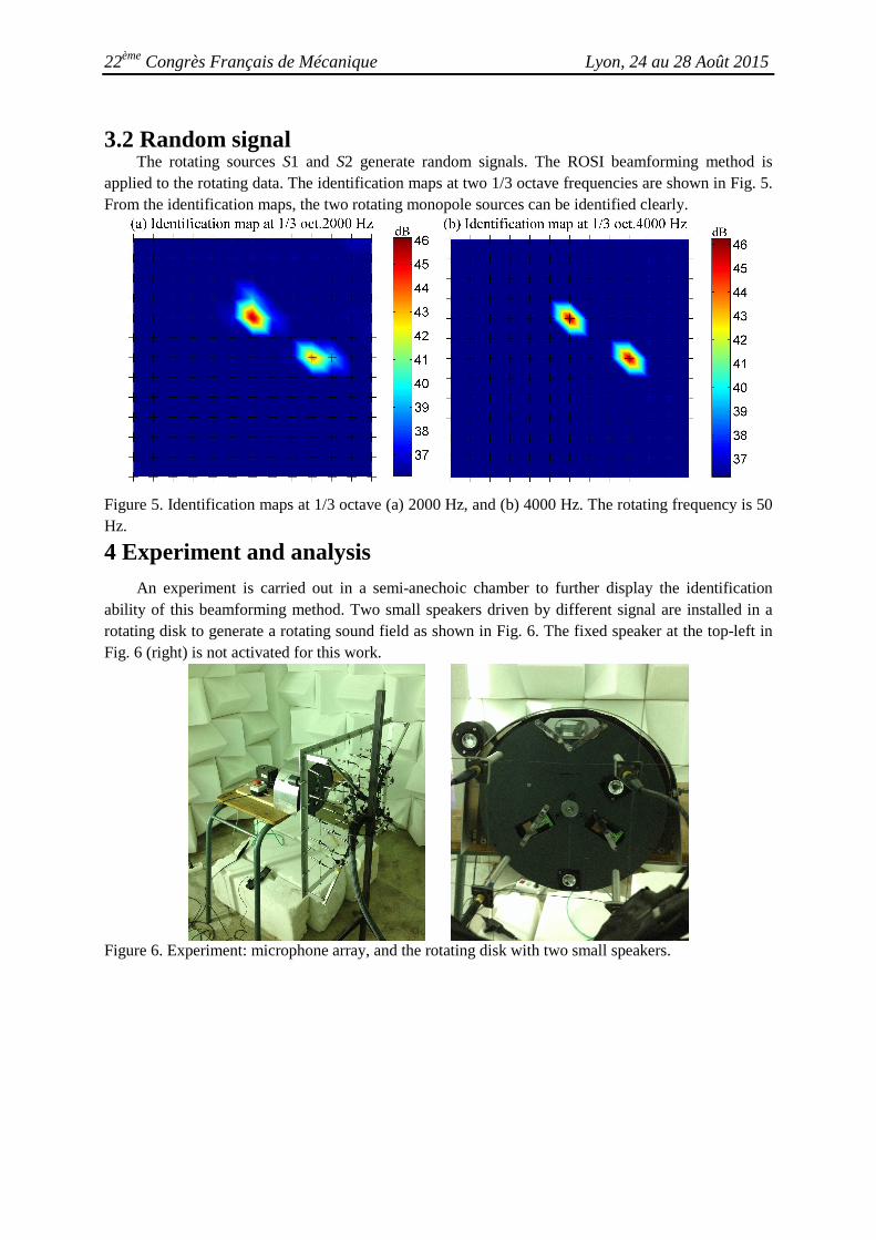
An experiment is carried out in a semi-anechoic chamber to further display the identification ability of this beamforming method. Two small speakers driven by different signal are installed in a rotating disk to generate a rotating sound field as shown in Fig. 6. The fixed speaker at the top-left in Fig. 6 (right) is not activated for this work.

Figure 6. Experiment: microphone array, and the rotating disk with two small speakers.


Figure 7. Geometry of the rotating disk with two small speakers, the measurement plane H, and the

focusing plane E in the Cartesian coordinate system ),,( zyxo .

The geometry of the rotating disk with two small speakers, the measurement plane H, and the focusing plane E is shown in Fig. 7. The initial center locations of the two small speakers are (0 m, 0.115 m, 0 m) and (0.065 m, 0.0375 m, 0 m), respectively. The measurement plane H is located at

z=0.15 m in the Cartesian coordinate system ),,( zyxo . The measurement plane H provides 5× 6

measured points and the grid spacing is 0.1 m in both x and y directions. The focusing plane E with 17× 21 points is located at =z 0 m and the grid spacing is 0.025 m in both x and y directions. The rotating frequency is set as 15 Hz, and the rotation speed is measured with an optical tachometer. The pressure signal is measured with a sampling frequency of 25.6 kHz, providing 5120 sampling points.

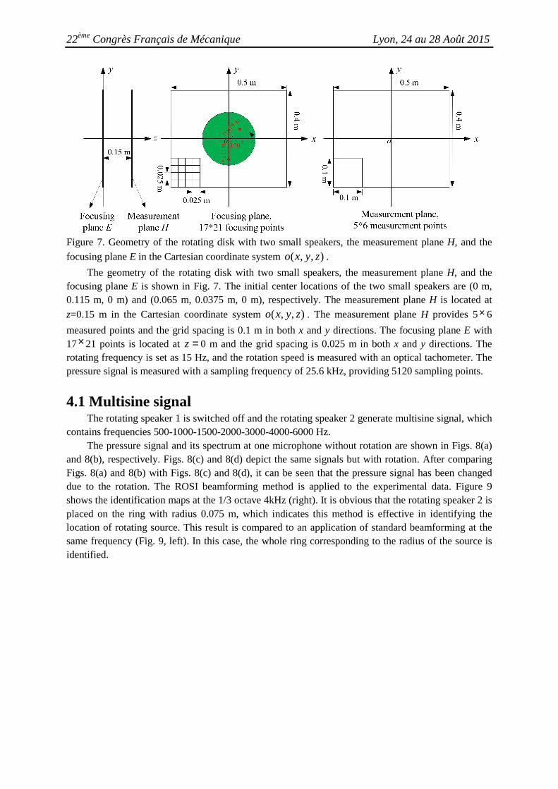
4.1 Multisine signal The rotating speaker 1 is switched off and the rotating speaker 2 generate multisine signal, which

contains frequencies 500-1000-1500-2000-3000-4000-6000 Hz. The pressure signal and its spectrum at one microphone without rotation are shown in Figs. 8(a)

and 8(b), respectively. Figs. 8(c) and 8(d) depict the same signals but with rotation. After comparing Figs. 8(a) and 8(b) with Figs. 8(c) and 8(d), it can be seen that the pressure signal has been changed due to the rotation. The ROSI beamforming method is applied to the experimental data. Figure 9 shows the identification maps at the 1/3 octave 4kHz (right). It is obvious that the rotating speaker 2 is placed on the ring with radius 0.075 m, which indicates this method is effective in identifying the location of rotating source. This result is compared to an application of standard beamforming at the same frequency (Fig. 9, left). In this case, the whole ring corresponding to the radius of the source is identified.


Figure 8. (a) Pressure signal at one microphone without rotation and (b) its spectrum signal, and (c) pressure signal at one microphone with rotation and (d) its spectrum signal.

Figure 9. Multisine signal, identification maps at 1/3 octave 4000 Hz, with standard beamforming (left) and with ROSI (right). The rotating frequency is 15 Hz. The green circle corresponds to the radial position of the loudspeaker. The initial angle for ROSI is chosen to match the angular position of the source in figure 6.

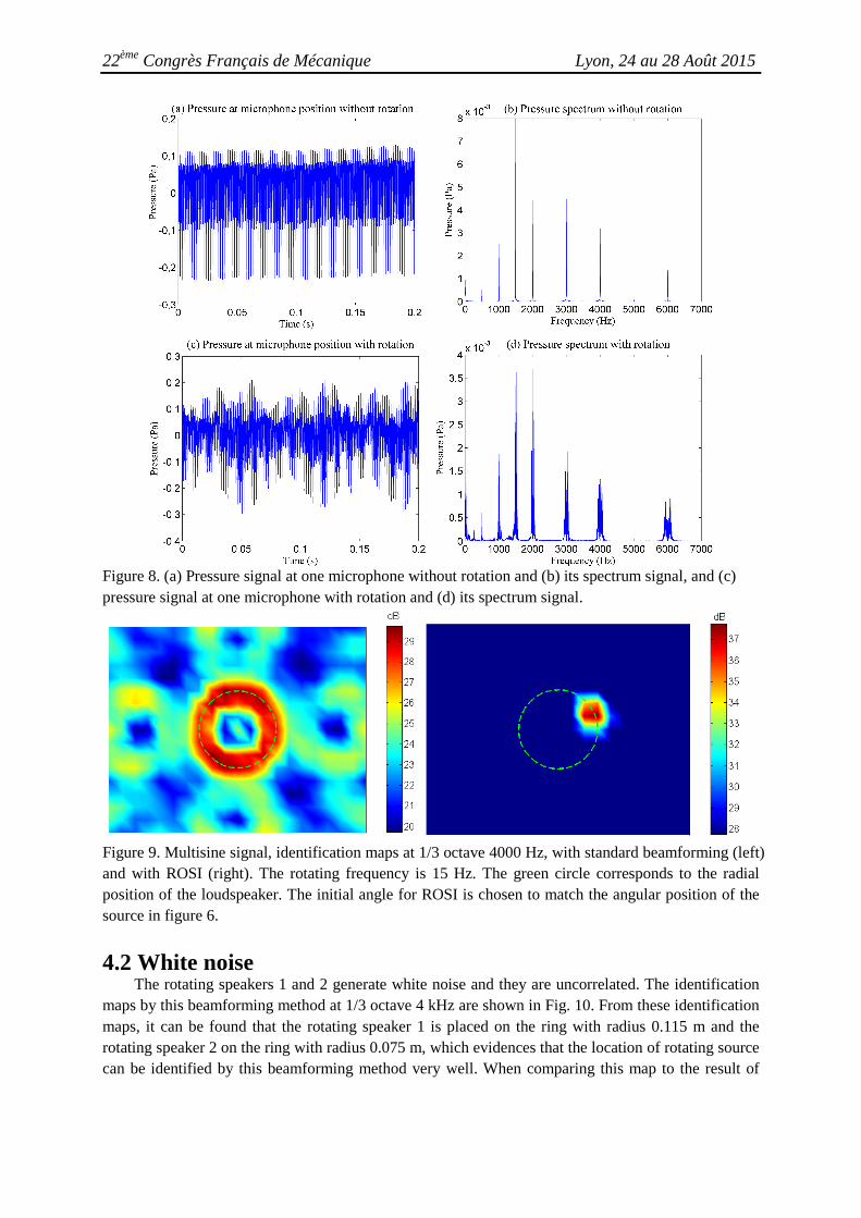
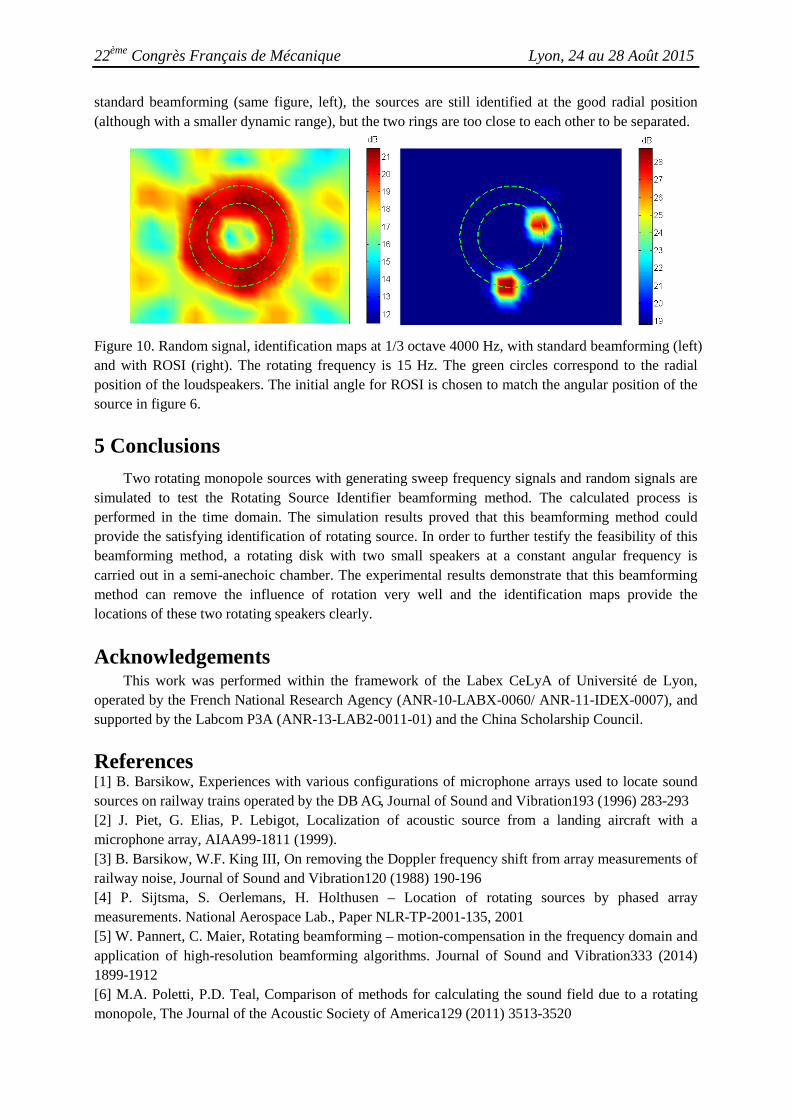
4.2 White noise The rotating speakers 1 and 2 generate white noise and they are uncorrelated. The identification

maps by this beamforming method at 1/3 octave 4 kHz are shown in Fig. 10. From these identification maps, it can be found that the rotating speaker 1 is placed on the ring with radius 0.115 m and the rotating speaker 2 on the ring with radius 0.075 m, which evidences that the location of rotating source can be identified by this beamforming method very well. When comparing this map to the result of


standard beamforming (same figure, left), the sources are still identified at the good radial position (although with a smaller dynamic range), but the two rings are too close to each other to be separated.

Figure 10. Random signal, identification maps at 1/3 octave 4000 Hz, with standard beamforming (left) and with ROSI (right). The rotating frequency is 15 Hz. The green circles correspond to the radial position of the loudspeakers. The initial angle for ROSI is chosen to match the angular position of the source in figure 6.

5 Conclusions

Two rotating monopole sources with generating sweep frequency signals and random signals are simulated to test the Rotating Source Identifier beamforming method. The calculated process is performed in the time domain. The simulation results proved that this beamforming method could provide the satisfying identification of rotating source. In order to further testify the feasibility of this beamforming method, a rotating disk with two small speakers at a constant angular frequency is carried out in a semi-anechoic chamber. The experimental results demonstrate that this beamforming method can remove the influence of rotation very well and the identification maps provide the locations of these two rotating speakers clearly.

Acknowledgements This work was performed within the framework of the Labex CeLyA of Université de Lyon,

operated by the French National Research Agency (ANR-10-LABX-0060/ ANR-11-IDEX-0007), and supported by the Labcom P3A (ANR-13-LAB2-0011-01) and the China Scholarship Council.

References [1] B. Barsikow, Experiences with various configurations of microphone arrays used to locate sound sources on railway trains operated by the DB AG, Journal of Sound and Vibration193 (1996) 283-293 [2] J. Piet, G. Elias, P. Lebigot, Localization of acoustic source from a landing aircraft with a microphone array, AIAA99-1811 (1999). [3] B. Barsikow, W.F. King III, On removing the Doppler frequency shift from array measurements of railway noise, Journal of Sound and Vibration120 (1988) 190-196 [4] P. Sijtsma, S. Oerlemans, H. Holthusen – Location of rotating sources by phased array measurements. National Aerospace Lab., Paper NLR-TP-2001-135, 2001 [5] W. Pannert, C. Maier, Rotating beamforming – motion-compensation in the frequency domain and application of high-resolution beamforming algorithms. Journal of Sound and Vibration333 (2014) 1899-1912 [6] M.A. Poletti, P.D. Teal, Comparison of methods for calculating the sound field due to a rotating monopole, The Journal of the Acoustic Society of America129 (2011) 3513-3520

Documents

Identification of rotating sound source based on