Identification of the cloud base height over the centra l H ... 1 Identification of the cloud base height over the centra l 2 H imalayan region: Intercomparison of Ceilometer and Doppler

1

Identification of the cloud base height over the central 1

Himalayan region: Intercomparison of Ceilometer and Doppler 2

Lidar 3

4

5

K.K. Shukla1, 2

, K. Niranjan Kumar3, D.V. Phanikumar

1, Rob K Newsom

4, V. R. Kotamarthi

5 6

Taha B.M.J. Ouarda3, 6

and M. Venkat Ratnam7 7

8

1Aryabhatta Research Institute of observational sciences, Nainital, India 9

2Pt. Ravishankar Shukla University, Raipur, Chhattisgarh, India 10

3Institute Center for Water and Environment, Masdar Institute of Science and Technology, Abu Dhabi, United Arab 11

Emirates 12 4Pacific Northwest National Laboratory, Richland, Washington, USA 13

5Argonne National Laboratory, Argonne, Illinois, USA

6INRS-ETE, Quebec City (Qc), Canada 14

7National Atmospheric Research Laboratory, Gadanki, Tirupati, India 15

16

Correspondence to: D V Phanikumar ([email protected]; [email protected]) 17

18

Abstract. We present the measurement of cloud base height (CBH) derived from the Doppler Lidar (DL), 19

Ceilometer (CM) and Moderate Resolution Imaging Spectroradiometer (MODIS) satellite over a high altitude 20

station in the central Himalayan region for the first time. We analyzed six cases of cloud overpass during the 21

daytime convection period by using the cloud images captured by total sky imager. The occurrence of thick clouds 22

(> 50%) over the site is more frequent than thin clouds (< 40 %). In every case, the CBH indicates less than 1.2 km, 23

above ground level (AGL) observed by both DL and CM instruments. The presence of low level clouds in the 24

height-time variation of signal to noise ratio of DL and backscatter of CM shows a similar diurnal pattern on all 25

days. Cloud fraction is found to be maximum during the convective period. The CBH estimated by the DL and CM 26

showed reasonably good correlation (R2=0.76). The DL observed updraft fraction and cloud base vertical velocity 27

also shows good correlation (R2=0.66). The inter-comparison between DL and CM will have implications in filling 28

the gap of CBH measurements by the DL, in absence of CM. More deployments of such instruments will be 29

invaluable for the validations of meteorological models over the observationally sparse Indian regions. 30

31

Key words: Cloud base height, Doppler Lidar, Celiometer, Radiosonde 32

33

34

35

Atmos. Meas. Tech. Discuss., doi:10.5194/amt-2016-162, 2016Manuscript under review for journal Atmos. Meas. Tech.Published: 13 July 2016c© Author(s) 2016. CC-BY 3.0 License.

2

1. Introduction 1

2

The Earth‟s shortwave and longwave radiation at the surface and as well as the top of the atmosphere is influenced 3

by cloud microphysical properties such as cloud coverage and cloud base height (CBH) (Considine et al., 1997; 4

Meerkӧtter and Bugliaro, 2009). The formation of all weather clouds occurs in lowest layer of the atmosphere (i.e. 5

troposphere). The extensive occurrence of stratocumulus and stratus clouds over ocean (~34%) and land surface 6

(~18%) in the lower atmosphere and near the atmospheric boundary layer (ABL) is well documented (Heymsfield, 7

1993; Considine et al., 1997). It was found that there is an increase in planetary albedo and a decrease in shortwave 8

radiation at the surface due to ABL clouds (Heymsfield, 1993; Berg and Kassianov, 2007). Moreover, clouds can 9

also affect the structure of atmospheric parameters like ABL height, temperature and relative humidity because of 10

their vital role in altering the water cycle over the Earth‟s surface and play a critical role in the removal of 11

atmospheric pollutants through precipitation (Ghate et al., 2011). 12

A strong coupling is observed between the fair weather ABL cumulus clouds and associated turbulence in 13

the ABL, which have impact on the ABL diurnal variability (Brown et al., 2002). These clouds can be lifted more 14

than a few hundred meters due to the ABL evolution during morning to the afternoon hours over the land 15

(Meerkӧtter and Bugliaro, 2009). The cloud top height can be retrieved with different retrieval algorithms (Forsythe 16

et al., 2000; Hutchison, 2002; Huang et al., 2006; Weisz et al., 2007) for use with various satellite observations such 17

as the Cloud-Aerosol Lidar and Infrared Pathfinder Satellite Observations (CALIPSO) (Winker et al., 2003), 18

CloudSat and Tropical Rainfall Measuring Mission (TRMM) (Stephens et al., 2002; Kummerow et al., 1998). 19

Due to the various feedbacks between clouds, radiation and dynamics described above, it is extremely 20

important to have the simultaneous observations of the fair weather cumulus clouds and vertical velocity in the 21

Earth‟s atmosphere for the appropriate representation in the Global Circulation Models (GCMS) (Randall et al., 22

1985; Tonttila et al., 2011). The vertical structure of convective and cumulonimbus clouds are studied by using 23

precipitation radar over the south Asian region (Bhat and Kumar, 2015). Sharma et al., (2016) studied the CBH 24

observed by using Ceilometer (CM) during 2013-2015 over the western site in India and also compared with the 25

Moderate Resolution Imaging Spectroradiometer (MODIS) satellite. The observed CBH by ground-based 26

(ceilometer) and space-based satellite (MODIS) observations are showing good correlation over the western Indian 27

site. 28

In addition, observations of vertical velocity remain sparse over most of the site in the Indian region and in 29

particular over regions with the high altitude and complex topography. The atmospheric radiation measurements 30

(ARM) Mobile Facility (AMF1) conducted a field campaign during June 2011-March 2012 over a high altitude site 31

Manora Peak (29.4o N; 79.2

o E; 1958 m amsl), Nainital to have a better understanding about the cloud, precipitation 32

and aerosols in the Ganges basin, i.e. Ganges Valley Aerosol eXperiment (GVAX). During GVAX, different ground 33

based remote sensing instruments were operated to measure the atmospheric dynamical parameters. A Doppler Lidar 34

(DL) was continuously operated to measure the vertical velocity and backscatter from the fair-weather ABL clouds. 35

Along with the DL, CM and Total Sky Imager (TSI) were also operated continuously to measure CBH and to 36

capture the cloud images, respectively, in the daytime over the observational site. 37


3

In the current study, our main objective is to evaluate the capability of DL in estimating the CBH and 1

comparing the results with CM, the standard instrument for the CBH measurement and CBH derived from the 2

MODIS. The advantage of DL over the other two measurements is that one can get the simultaneous information on 3

both vertical velocities near clouds along with the CBH. In this study, we have considered six selected cases based 4

on cloud coverage, residence time of clouds and availability of simultaneous datasets with other ground based 5

instruments over the site during the observational period (05-10 UT). 6

7

2. Observational site, instrumentation and methodology 8

9

Ganges valley region of the Indian subcontinent is a heavily populated region and shows an increase in the 10

pollutants level in the current climate (Ramanathan et al. 2005; Lau and Kim 2006; Bollasina et al., 2011). Bollasina 11

et al., (2011) showed the increment in the concentration of anthropogenic aerosols over the Ganges valley region 12

which has the ability to modify the Indian Summer Monsoon (ISM) rainfall. To understand climate change over the 13

Indo-Gangetic Plain (IGP), the geographical location of Manora Peak (29.4o N; 79.2

o E; 1958 m amsl), Nainital is 14

suitable for measuring the various atmospheric parameters in campaign mode. To have a better understanding of the 15

impact of measured parameters like aerosol, convection, cloud, and radiative characteristics of the Indian monsoon, 16

Atmospheric radiation measurement (ARM) mobile facility conducted a field campaign over the site which is 17

known as Ganges Valley Aerosol Experiment (GVAX) (Kotamarthi, 2010). The GVAX campaign was utilized to 18

quantify the impact of aerosols on ISM, role of atmospheric boundary layer in aerosol transportation in the Ganges 19

valley region and also the effect of aerosols in the cloud formation. By considering all the above serious issues, the 20

current observational site is selected to conduct the campaign mode observations (Kotamarthi, 2013). 21

The observational site Manora Peak, Nainital is located in the central Gangetic Himalayan region and is 22

considered as a high altitude site in the northern part of the Indian region. It is away from the urban/industrial 23

pollution. The total population of the Nainital is ~ 0.5 million (according to census 2011) with population density ~ 24

50 persons per km2. The small-industries having cities i.e. Haldwani and Rudrapur are located ~20-40 km away in 25

the south of the observational site. A mega city, New Delhi, the capital of India is located ~ 225 km in the southwest 26

of the study region (Sagar et al., 2015). The site is surrounded by a dense forest. The maximum and minimum 27

temperatures are observed to be ~ 20 0C and 1

0C during pre-monsoon (March April May) and winter (December 28

January February) seasons, respectively (Dumka et al., 2014; Shukla et al., 2014). Moreover, wind patterns over the 29

site during monsoon and winter are southwesterly and northwesterly, respectively. The seasonal change in wind 30

pattern every year persists over the Indian subcontinent (Asnani, 2005). The detailed description about the site and 31

current research works carried out over the observational site can be found in detail in Sagar et al. (2015). 32

33

2.1 Total Sky Imager (TSI) 34

The TSI is manufactured by Yankee Environmental Systems (YES), and is commercialized version of the 35

hemispheric Sky Imager prototype (Long et al., 2006). The TSI 440/660 was deployed over the Manora Peak, 36


4

Nainital during the GVAX to capture the cloud images during the daytime. The sky cloud images captured by TSI 1

are 24-bit color JPEG images at 352x288 pixel resolution. TSI captures the cloud image at every 30 sec during 2

daytime. In order to retrieve cloud information, we have processed the raw cloud images of the TSI. Sky cover 3

retrieval from TSI images is valid only for solar elevation angles >100 (zenith angles < 80

0) and images are 4

processed for a 1600 field of view, ignoring the 10

0 of sky near the horizon. It has a sun-blocking strip mask, which 5

represents the location of the sun with a yellow dot in the image. We have used TSI images to infer the presence of 6

clouds over the site for a subsequent CBH estimate. The TSI observations of cloud images are also utilized for the 7

estimation of percentage of thin and opaque clouds over the site. The detailed discussion about the estimation of 8

cloud properties by using TSI images are given somewhere else in previous reports (Long et al., 2001, 2006; Morris, 9

2005). 10

11

2.2 Doppler Lidar 12

13

DL was operated over a high altitude site to measure the temporal and altitude resolved vertical velocity and 14

attenuated backscatter. In order to retrieve the radial velocity by using Doppler principle, DL uses aerosols as tracer 15

in the atmosphere to observe the Doppler shift. The influence of insects or pollen is less in the DL observations 16

because the small aerosols in the background dominate the signal. The DL uses an eye-safe laser of wavelength ~1.5 17

µm. It provides the vertical velocity and attenuated backscatter at a spatial resolution of ~30m and a temporal 18

resolution of 1 sec. The DL can scan the atmosphere in different modes (i.e. vertically Fixed-Beam Stare (FPT), 19

Range-Height Indicator (RHI) scan and Plan-Position Indicator (PPI) scan mode). The RHI and PPI scan modes are 20

known as the elevational and azimuthal scan of the atmosphere, respectively. A detailed technical description of the 21

DL system can be found in previous studies (Pearson et al., 2009; Newsom, 2012; Shukla et al., 2014). In the current 22

study, the vertically fixed-beam stare mode of the DL is used to estimate CBH. To minimize/remove random noise 23

fluctuations in the DL data, a threshold on signal to noise ratio (SNR) of -20 dB is applied. 24

25

2.3 Laser Ceilometer 26

27

The Väisälä laser Ceilometer (CT25K) is deployed over the site for precise measurements of the CBH, vertical 28

visibility and vertical profile of aerosol backscatter during GVAX (Väisälä Oyj, 2002). It has an eye-safe laser 29

source of wavelength ~905 nm. It provides the information at a temporal resolution of 16 sec and a spatial resolution 30

of 30 m in the atmosphere (Morris, 2012). The 16 sec interval data is aggregated to 1 min for better comparison with 31

the DL. 32

33

2.4 Surface Meteorology System 34

35

The in-situ sensors are used to measure the surface temperature (T), relative humidity (RH), pressure, wind speed 36

and wind direction by the ARM surface meteorology systems (MET). The in-situ sensors are installed at specific 37


5

standard heights for measurement of meteorological parameters (i.e. T & RH at 2 m; Barometric pressure at 1 m and 1

wind speed and direction at 10 m) (Ritsche and Prell, 2011). The MET sensors provide the data at a temporal 2

resolution of 1-min and we have averaged for 10-min from 1-min data to calculate the lifted condensation level 3

(LCL) for comparison with the CBH of DL and CM, respectively. 4

5

2.5 Radiosonde 6

7

Väisälä Radiosondes (RS-92) were launched during GVAX at 00, 06, 12 and 18 UT daily regularly. The profiles of 8

atmospheric parameters (temperature, relative humidity and winds) are measured by the Radiosonde (RS) at a 9

vertical resolution of 10 m as the ascent rate of balloon is 5 ms-1

and transmitter time resolution is 2 sec. In the 10

current study, we have used the 06 UT (11.5 hr LT) data of RS to calculate the LCL for all the cloud cases. The 11

detailed description about the RS can be found in previous reports (Holdridge et al., 2011; Shukla et al., 2014). 12

13

2.6 Moderate resolution imaging spectroradiometer 14

15

In addition to the ground based remote sensing techniques used for the estimation of CBH, we have also utilized the 16

MODIS satellite derived CBH over the observational site. The MODIS Terra data is obtained for the same cases as 17

measured by the ground based remote sensing instruments. However, the spatial resolution of MODIS cloud data is 18

of 10 x 1

0 latitude-longitude grids. We have used the cloud top pressure, cloud optical depth and effective radius of 19

liquid cloud for all the cases. 20

21

3. Retrieval of Cloud base height (CBH) and Lifting Condensation Level (LCL) 22

23

3.1 Cloud Statistics from the DL 24

25

We have used the vertical velocity and cloud statistics derived data of the DL during GVAX (Newsom et al., 2015). 26

In addition to clear-air vertical velocity statistics, we can derive the CBH, cloud fraction, cloud base vertical velocity 27

and cloud base updraft fraction. For the current data set, the averaging interval was 30 min oversampled for every 10 28

min. The cloud fraction is the fraction of time during the averaging interval that a cloud is detected at any height. 29

Similarly, the cloud base updraft fraction is the fraction of time that a positive (upward) cloud base vertical velocity 30

is observed during the averaging interval. 31

CBH estimates are obtained from the 1-sec DL data by detecting the heights of sharp spikes in the range-32

corrected SNR. In order to identify the cloud bases, the DL uses a narrow Gaussian filter in the scattered signal due 33

to the presence of clouds in the atmosphere. The Gaussian filter is convolved with each SNR profile to detect the 34

cloud base. To minimize false detections, the CBH algorithm uses a method based on the first derivative of the 35

range-corrected SNR. First, the range-corrected SNR profiles are differentiated using a simple central-difference 36

approximation. When a cloud is present in the profile, the first derivative shows a strong positive peak immediately 37


6

below and a strong negative peak immediately above the cloud base. The algorithm then locates the maximum in the 1

range-corrected SNR between these two extrema. Additional checks are applied to minimize false detections by 2

rejecting temporally isolated peaks. The cloud base vertical velocity is then simply the vertical velocity at the CBH. 3

The vertical velocity and cloud statistics derived from the DL reports the median CBH and the median cloud base 4

vertical velocity over a given 30-min averaging interval. Further details are given in Newsom et al. (2015). 5

6

3.2 CBH retrieval by using CM 7

8

The measurement of the CBH with CM is known as standard method of the ground-based active remote sensing 9

technique. The time delay between the transmitted and backscattered signal from the haze, fog, virga, mist and 10

precipitation to the receiver of CM can be used to estimate the CBH. By knowing the time delay in equation (1), 11

CBH can be estimated as 12

Cloud base height (h) = (c*t/2) (1) 13

where c (= 3 x 108 m s

-1) is the speed of light and t is the time delay. The backscattering coefficient is estimated by 14

using the strength and attenuation of the backscattered signal from the atmosphere. Cloud base is identified by the 15

strong increase of the backscatter coefficient and three layers of clouds can be detected if the lower clouds are 16

transparent (Emeis et al., 2009; Morris, 2012). 17

18

3.3 CBH Retrieval by MODIS 19

20

The CBH from the MODIS is calculated by taking the difference between the cloud top height and the thickness of 21

cloud (∆Z) which is given in equation (2). 22

ZCloud base height = ZCloud top height - (∆Z) (2) 23

where ∆Z is the cloud thickness and ∆Z is ratio of LWP and LWC. 24

The thickness of water cloud depends on the relation between liquid water path (LWP) and liquid water 25

content (LWC). Liou (1992) showed that the relation of cloud optical thickness (τ) and effective radius of cloud 26

particle size (reff) with LWP is given by 27

LWP= (2* τ* reff)/3 g.m-2

(3) 28

LWC=0.26 g.m-3

taken for cumulus cloud in clean condition (Hess et al., 1998). 29

∆Z= (LWP/LWC) (4) 30

By using LWP & LWC in equation (4), we have calculated the thickness of cloud (∆Z). 31

We have estimated the CBH for water cloud present in the atmosphere by using equation (2) & (4). Based 32

on the method described by Hutchison (2002) and Sharma et al., (2016), we have used the cloud top pressure and 33

liquid water path during daytime from MODIS Terra satellite over the observational site for cloud passages 34

observed by the TSI. 35

36

37


7

3.4 Lifted condensation level estimation by using surface MET and RS datasets 1

2

The estimation of water vapor content from surface MET data has been derived by using equation (5) with T and 3

RH of surface meteorology (Goff-Gratch, 1946). 4

es=est * 10Z (5)

5

where 6

7

8

and A = -7.90298, B= 5.02808, C=-1.3816 X 10-7

, D= 11.344, F=8.1328 X 10-3

, H= -3.49149 are the constants. est 9

(=1013.246 mb) is saturation vapor pressure (es) at boiling temperature (Ts=373.16 K) at standard atmospheric 10

pressure. By using saturation vapor pressure (es) from equation (5) and surface RH in equation (6), we have 11

calculated the water vapor pressure (e) 12

(6) 13

Dew point temperature (Td) estimation by using surface MET vapor pressure (e) is given by the equation (7) 14

(7) 15

where T0=273 K, eo = 0.611 kPa, , e - vapor pressure 16

By knowing the temperature (T) and dew point temperature (Td) from surface meteorology and RS, we have 17

calculated LCL by using equation (8) 18

Lifting Condensation level (LCL) height (km) = 0.125* (T-Td) (8) 19

20

4. Results and discussion 21

22

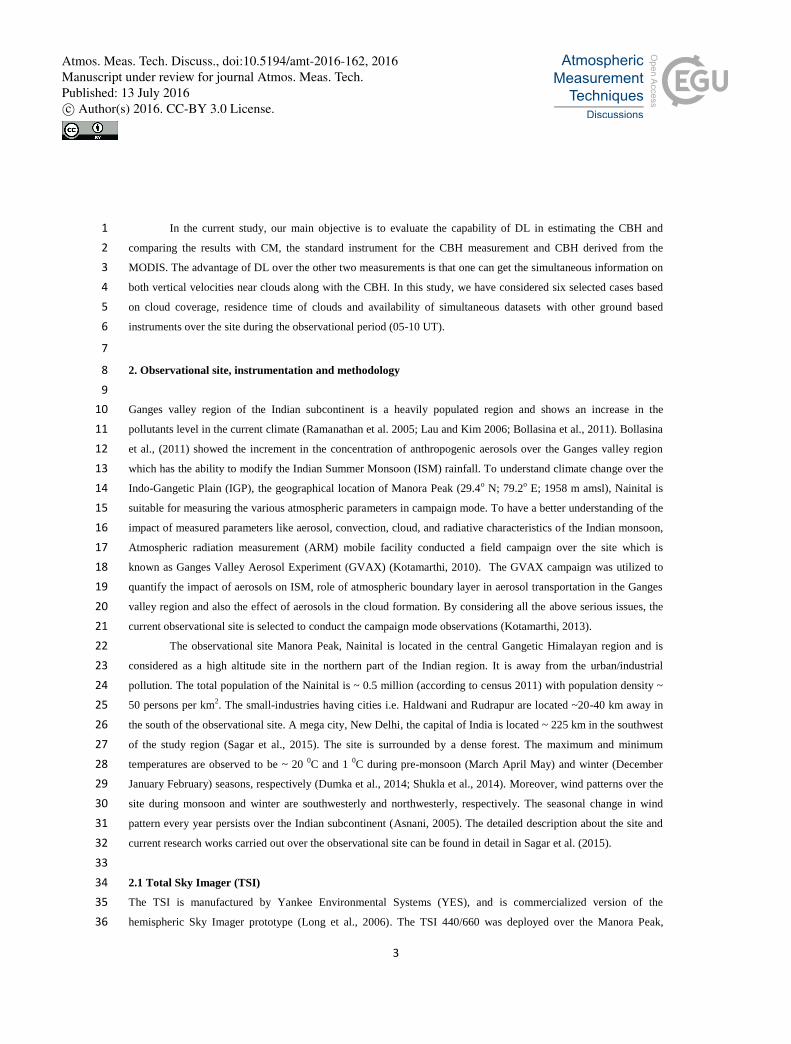
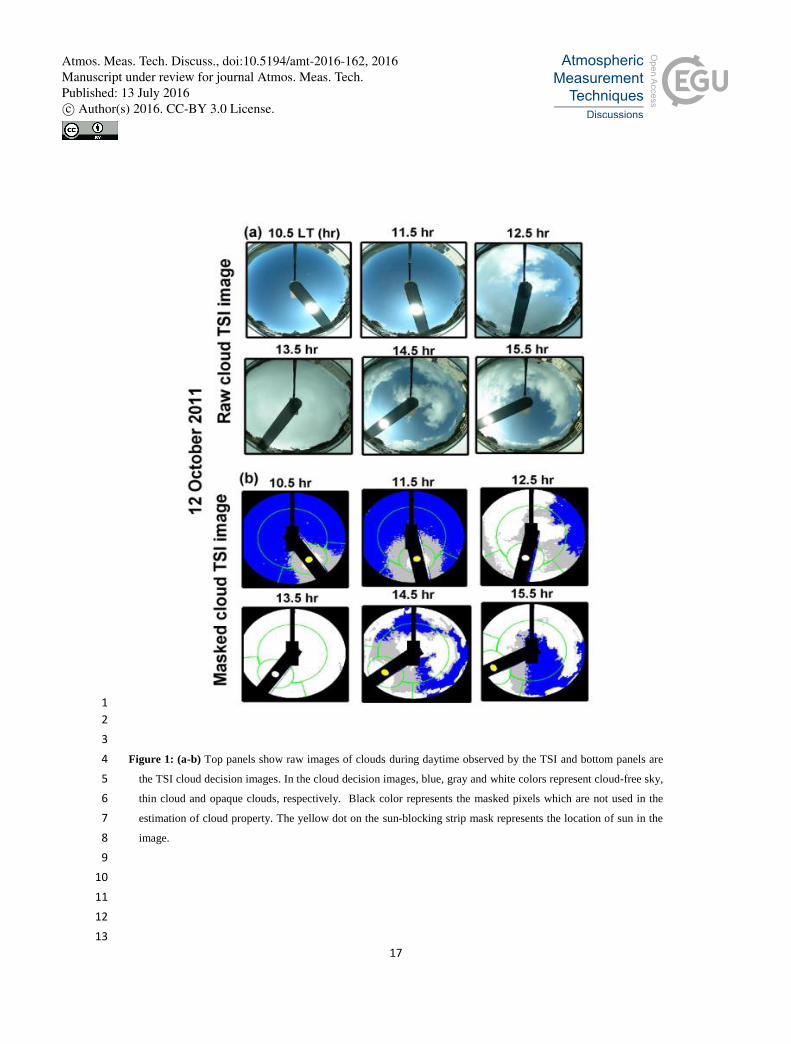
Figure 1 shows one of the six (12 October 2011, 21 November 2011, 11 December 2011, 20 January 2012, 08 23

February 2012 and 14 March 2012) cloud case examples considered in this study observed by TSI for the estimation 24

and comparison of CBH by different instruments over the observational site. It shows the raw (Figure 1a) and 25

masked (Figure 1b) cloud images by TSI at hourly interval during daytime from (10.5-15.5 hr) on 12 October 2011. 26

The “yellow dot” in the TSI masked image represents the position of the sun, not obscured by the clouds. However, 27

if this “yellow dot” becomes “white” then the sun is obscured completely by the clouds (Figure 1b; Pfister et al., 28

2003). It is also to be noted that the presence of cloud is clearly apparent with the raw image of the sky captured by 29

TSI (Figure 1a). However, the masked images strongly confirm the presence of clouds and further distinguish 30

between the thin and opaque clouds by the color of the image. For instance, the blue, gray, and white colors in 31


8

Figure 1b represent the cloud free-sky, thin and opaque clouds, respectively. While the black color in Figure 1b 1

represent the masked pixels which are not used in determining the microphysical property of cloud by the TSI. 2

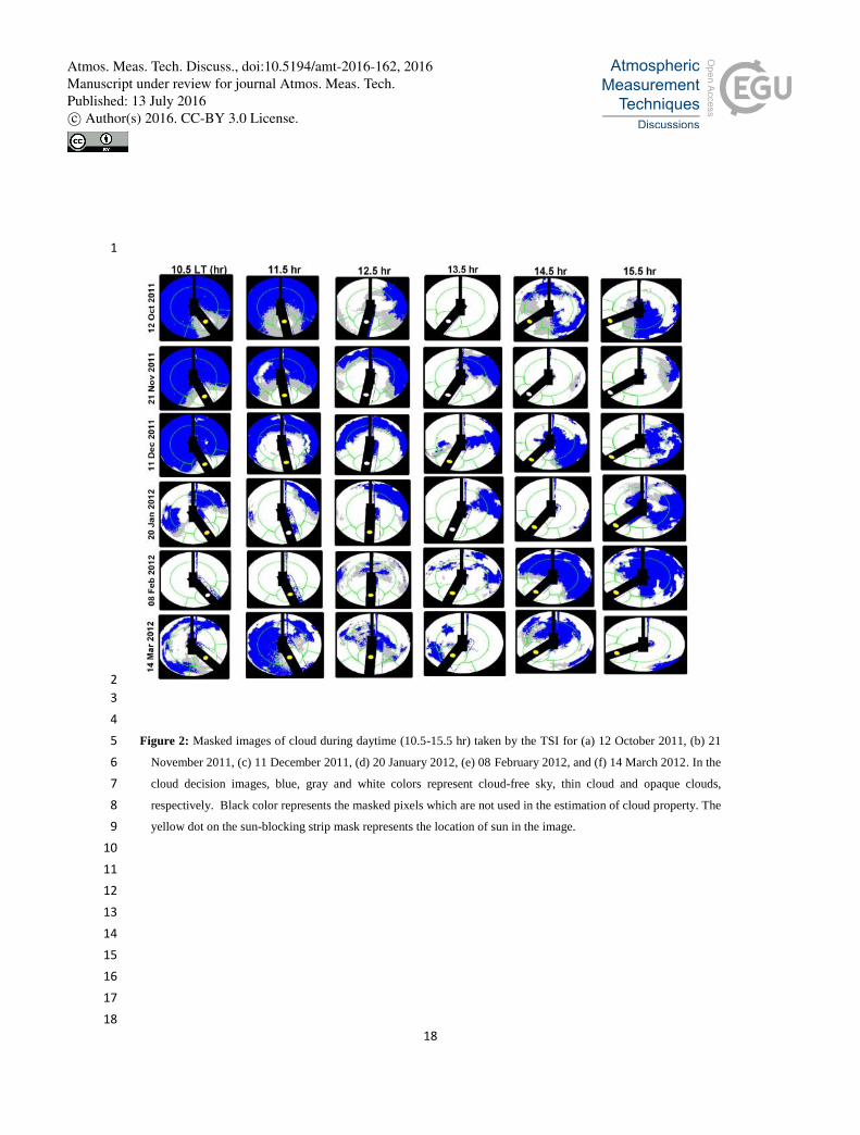
Temporal variation of masked images of clouds captured by TSI for all cases in the 1600 field of view 3

(FOV) centered at zenith in the cloud images during 10.5-15.5 LT is shown in Figure 2. Due to masked sky images, 4

the loss of about 17 % of the hemispherical solid angle of the sky dome is resulted. In the analysis of clear/cloudy 5

pixels, these masked „black‟ parts are ignored (Long et al., 2006). From Figure 2, it is clearly seen that there are 6

lesser clouds in the forenoon (before 12.5 LT) in comparison to afternoon (after 12.5 LT) on 12 October, 21 7

November and 11 December 2011. We have observed the clouds at every hour on 20 January, 08 February and 14 8

March 2012. 9

In Figure 3 (a-f), we also show the temporal variation of the percentage occurrence of thin (shown by black 10

line with black open circle) and opaque clouds (red line with red open rectangle) for all the six cloud overpasses 11

over the observational site. To classify the thin and opaque clouds, we have performed the red-green-blue (RGB) 12

pixel classification of the cloud images. The scattering of blue light is more than red in clear skies and no aerosols 13

conditions (i.e. molecular scattering). If cloud is present in the atmosphere then red pixel value is greater than where 14

no clouds. 15

For clouds the relative ratio of red/blue pixel is greater than clear sky. Koehler at al. (1991) developed the 16

cloud decision threshold (red/blue ratio) algorithms for thin and opaque clouds for the first time from the TSI. If the 17

relative red/blue ratio of the pixel is higher than 0.6 then it is categorized as cloudy and lesser values are marked as 18

cloud free. The detailed descriptions about the classification of thin and opaque clouds are given in Slater et al., 19

(2001). In most of the cases of figure 3(a-f), the percentage of opaque clouds are greater than percentage of thin 20

clouds. The dominance of opaque clouds is clearly seen from the figure 3(a-f) during afternoon (12.5 LT) hours over 21

the site. It is also evident from Figure 3 that the percentage occurrence of opaque clouds is more frequent over the 22

site relative to the thin clouds during the observational period. 23

Figures 4 (a1-f1) and (a2-f2), illustrate the height-time variation of SNR and backscatter for different cases 24

of cloud passage over the observational site observed by DL and CM, respectively. Figure 4 depicts the presence of 25

ABL clouds over the site. The development of convective clouds in the lowest part of ABL is due to the presence of 26

convective thermals. These convective thermals are crucial in the formation of the clouds because these thermals can 27

rise from the surface to the top of the mixing layer without being diluted (Crum and Stull, 1987). It should be noted 28

that the presence of the convective clouds in the ABL can be confirmed by using the observed CBH from DL and 29

CM and lifted condensation level (LCL) estimated from the surface (Stull and Eloranta, 1985; Zhang and Klein, 30

2013). During the convection, the maximum SNR is observed due to the presence of low level ABL cumulus clouds. 31

Also, the observed cloud cases show different dynamics of the cumulus clouds over the site. Figure 4(a1) shows the 32

SNR maximum around 11.5-12.5 LT showing high percentage of opaque cloud during 12.5-14.5 LT and then 33

dominated by a thin clouds, consistent with Figures 4(a1) and 4(b1). Other cases also depict similar variation with 34

opaque clouds more frequent than the thin clouds during convection (see Figures 4b1-f1). Similarly, Figure 4 (a2-f2) 35

shows the height-time variation of averaged backscatter (srad-1

.km-1

.10-4

) by the CM observed for all cloud cases in 36


9

the study. It is interesting to note that the temporal evolution and duration of thin and opaque clouds in both the 1

instruments are in reasonable agreement during all events. 2

In Figure 5 (a-f), we have plotted the temporal variation of CBH (with DL & CM) and cloud occurrence 3

frequency (with DL). The detailed description about the estimation of CBH is given in the section 3.1. The 4

fraction of time that a cloud is detected at any altitude during the given averaging period is defined as cloud 5

frequency. Varikoden et al. (2011) showed that the occurrence of low level clouds are more in comparison to the 6

mid-level clouds by using CM over a tropical station Akkulam, Thiruvananthapuram (8.29◦ N, 76.59◦ E, 15 m 7

above sea level) in India. They have also showed that the occurrence of low level clouds is higher during the 8

afternoon hours. We have also found that the frequency of occurrence of clouds is higher during afternoon in the 9

observed cases with both CM and DL over a high altitude site. 10

Figure 6 depicts the temporal variation of CBH observed by the DL and CM along with lifted condensation 11

level (LCL) height estimated by using surface MET parameter and RS on (a) 12 October 2011 (b) 21 November 12

2011 (c) 11 December 2011 (d) 20 January 2012 (e) 08 February 2012 and (f) 14 March 2012. There is a strong co-13

relation between the CBH observed by the DL and CM for all cases. On an average, the CBH from both the 14

instruments is higher during the convective period and is associated with the change in LCL in the ABL during 15

daytime. ABL cloud heights are estimated by using LCL (Stackpole, 1967). The well-mixed ABL air parcels which 16

have a dry-adiabatic temperature profile and a constant mixing ratio are used to determine the LCL profile (Craven 17

et al., 2002). For the detection of CBH, the LCL is a good approximation as the CBH depends on the relative 18

humidity and temperature near the surface. The LCL depends on the temperature and dew point temperature above 19

the surface and thus a good proxy for CBH. We have estimated the LCL with surface MET and RS to compare with 20

the CBH of DL and CM. In 12 October 2011 case, a small difference is observed between the CBH (DL) and LCL 21

heights but LCL heights with the MET and RS shows a similar pattern as CBH (CM) implying the strong 22

association with ABL dynamics (Jones et al., 2011). From Figure 6 (a-f), it is clearly observed that in all the cases, 23

CBH is coupled with the LCL estimated from the surface meteorological parameters. This strong dependence of 24

CBH with LCL suggests the link between cloud formation and development of convection on the surface (Zheng et 25

al., 2015; Zheng and Rosenfeld, 2015). 26

In Figure 7, we have plotted the temporal variation of CBH with cloud base vertical velocity for all cases. 27

CBH observed with both the instruments are showing similar temporal variation throughout the observational time 28

period (10.5-15.5 LT). From figure 7(a-f), it is clearly evident that the updrafts are dominant due to the diurnal 29

evolution of convective ABL during daytime over the site. In some cases like 12 October 2011, 21 November 2011 30

and 08 February 2012, the vertical velocity follows the similar pattern. We have also plotted the temporal variation 31

of cloud base vertical velocity with cloud base vertical velocity updraft fraction (m) for all cases in Figure 8 (a-f). 32

From this figure, it is clearly seen that both the parameter are well correlated. 33

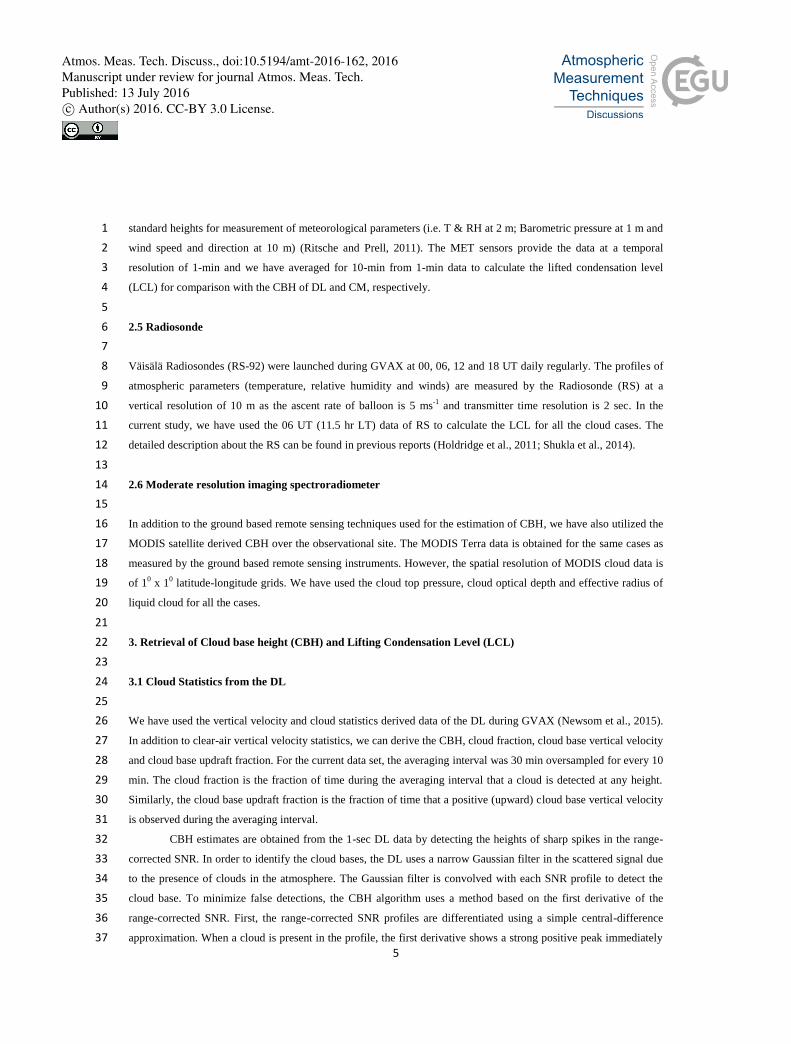
We have also compared the CBH calculated by the DL and CM with the MODIS derived CBH for all cloud 34

passes over the observational site. For instance, Figure 9 shows the MODIS Terra derived CBH and the daily mean 35

(05-10 UT) CBH measured by the DL and CM. We have taken the mean of latitude/longitude ± 1 degree by 36

centering the latitude/longitude of the observational site. The observed CBH from MODIS is well within the 37


10

estimated standard deviation from ground based CBH. It shows reasonably good agreement with the estimation of 1

CBH from the ground based and DL and CM CBH in all the cases except in two cases (21 November 2011 and 14 2

March 2012) where the differences are slightly higher and need to be investigated for the possible inconsistencies. 3

Further, we have used the DL and CM CBH as well as cloud updraft and cloud base vertical velocity 4

observed by the DL for all six cases to see the correlation which is plotted in Figure 10. The correlation of CBH 5

between the DL and CM is shown in Figure 10a. It is noticed that the CBH estimated by the DL is well correlated 6

(R2=0.76) with the CM measured CBH when we combine all the cases shown in Figure 10a. In addition, Figure 10b 7

illustrates the relation between cloud base vertical velocity and cloud updraft fraction observed by DL for all cloud 8

passes over the observational site. As indicated in Figure 10b, a strong correlation is also noted between these two 9

parameters. Further, it is noticed that when the cloud updraft fraction is less than 40%, the cloud base vertical 10

velocity tend to be negative. However, positive vertical velocities are noted when the cloud updraft fraction is more 11

than 50%. Kollias et al. (2001) showed that the cloud base vertical velocity is consistent with the updraft speed. We 12

have also observed similar behavior between the cloud base vertical velocity and updraft fraction although our 13

observations are from a high altitude location. 14

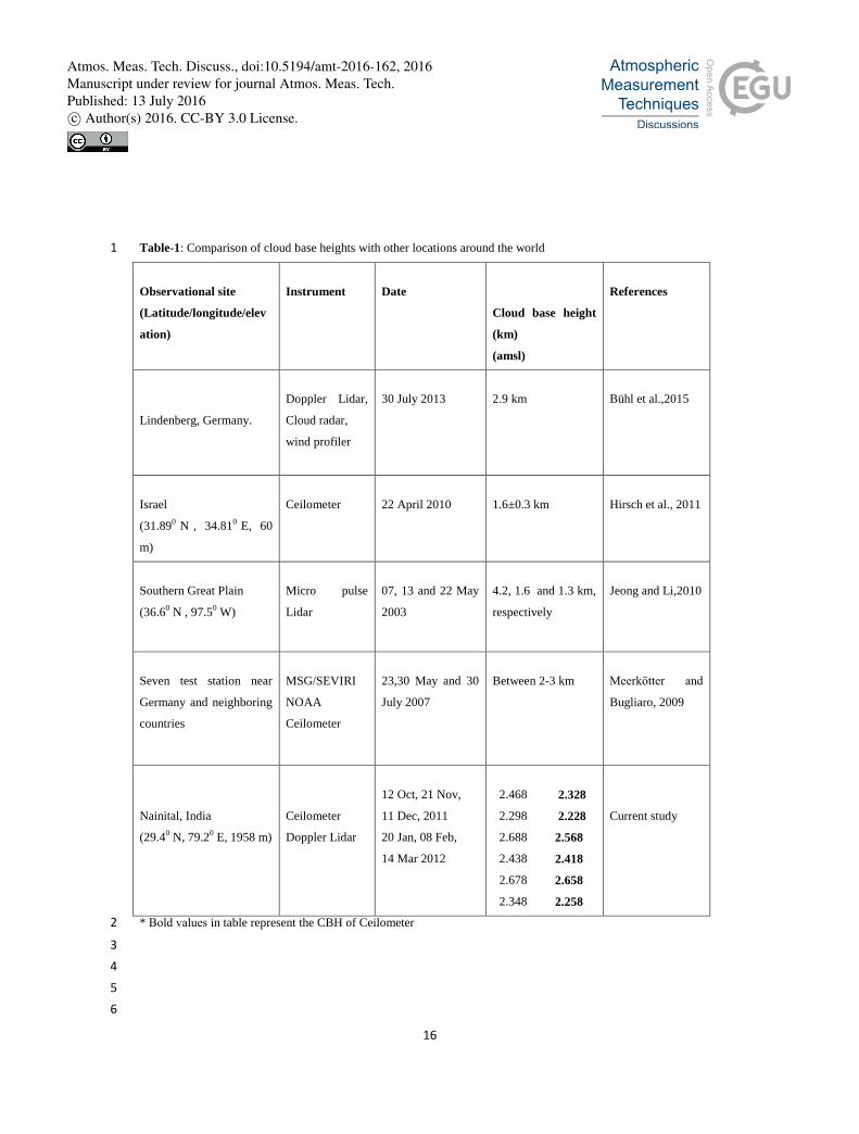
Jeong and Li (2010) estimated the CBH by using micropluse Lidar for few case studies by applying the 15

threshold condition of aerosol particle diameter less than 1 µm and relative humidity 40 % over the southern great 16

plain site. They have observed the cumulus cloud on all cases and found the CBH varying in between 1-4 km, above 17

mean sea level (amsl). A detailed comparison of CBH estimated over various parts of the world by using different 18

ground based instruments and satellite datasets is shown in Table-1. Despite different site morphologies, our CBH 19

values observed with both DL and CM (Table-1) are in agreement with past studies across the globe. Bühl et al., 20

(2015) observed the cloud and vertical velocity by using different ground based instruments e.g. DL, cloud radar and 21

wind profiler over meteorological observatory, Lindenberg, Germany. 22

The observations from all the instruments at this site with cloud layer overhead are ~3 km. The presence of 23

large-scale updrafts in the cloud layers was also observed. The observed vertical velocity in the cloud layer varied 24

between ± 1.5 ms-1

. Similar characteristics were observed at Manora Peak, Nainital. We have observed that cloud 25

base vertical velocity varies between ± 2 ms-1

except for 20 January 2012 during which higher vertical velocities of 26

0-4 ms-1

were obtained. The observed CBH also varies between 2.3-2.7 km amsl in both instruments over Manora 27

Peak, Nainital. Hirsch et al. (2011) retrieved the CBH by CM, and observed the shallow cumulus cloud during 28

daytime and CBH at 1.6±0.3 km, amsl. Also, Meerkӧtter and Bugliaro, (2009) estimated the CBH by using 29

MSG/SEVIRI, NOAA satellite data and CM data for convective cloud cases over the seven test stations near 30

Germany and neighboring countries. By using geostationary satellite and ground based CMs, they have observed 31

that CBH varies between ~ 2-3 km and also showed a significant correlation. Thus, our results are in good 32

agreement with the temporal variation of CBHs observed by DL compared with CM in previous studies. 33

34

5. Summary and Conclusions 35

In this study, we have presented comparison of the CBH estimated by using the DL with CM and MODIS derived 36

CBH over a high altitude site in the central Himalayan region. Total sky imager shows the presence of cloud over 37


11

the site for the cases evaluated in the current study and also opaque clouds are more frequently observed than thin 1

clouds over the site during the observational period. The height-time variation of signal to noise ratio of DL and 2

backscatter by the CM depict a similar pattern for the cases evaluated with opaque (thin) clouds dominating during 3

morning (afternoon) hours in most of the cases. Strong correlation (R2=0.76) between DL and CM CBH is observed 4

suggesting that DL can also be used as a potential instrument for measuring CBH apart from standard instrument 5

CM. Similarly, we have observed the good correlation (R2=0.66) between cloud base vertical velocity and cloud 6

updraft fraction. We have observed a similar temporal variation between CBH (estimated from DL and CM) and 7

LCL height (Surface MET and RS) during all the cases. The CBH height and LCL height derived from surface MET 8

and RS are also comparable. The estimated CBH with the MODIS data is also in close agreement with the ground 9

based instruments in most of the observed cases. 10

Further, our results also show close agreement with the CBH derived by DL, CM and MODIS derived satellite 11

data sets in all cases. Therefore, our results depict that DL is also a potential instrument for cloud studies apart from 12

standard CM instrument in measuring the CBH. The cooling and warming of the atmosphere is governed by the 13

presence of clouds at different altitudes in the atmosphere (Kiehl and Trenberth, 1997). CBH of low level clouds 14

coupled with shallow convection is playing an essential role in the parameterization of weather and climate models 15

(Chandra et al., 2015). Also the uncertainty observed in climate models is due to low-level clouds (Bony and 16

Dufresne, 2005) especially when model grid spacing is much larger than the size of low level. Therefore, the 17

continuous estimation of CBH will be a useful input for the models. Further, the cloud radiative cooling, relative 18

humidity in the ABL and cloud cover have direct association with the low altitude clouds (Brient and Bony, 2012). 19

Therefore, the accurate and systematic measurements of low level cloud base become important for the 20

improvement of the models. 21

Hence, in this report we investigated the potential of the DL in measuring the CBH over the site in comparison 22

to CM. From the current study, it is also clearly seen that we can use DL for CBH study over the site. It also 23

demonstrates that the precise observations of the CBH over the complex topography are very useful for model 24

validation. By considering the importance of the current study, CBH estimations by DL along with the cloud updraft 25

velocities will be utilized in our future studies as potential inputs for numerical weather prediction models over the 26

Central Himalayan region. 27

28

Acknowledgments 29

30

This work has been carried out as a part of GVAX campaign under joint collaboration among Atmospheric 31

Radiation Measurement (ARM), Department of Energy (US), Indian Institute of Science (IISc) and Indian Space 32

Research Organization (ISRO), India. We thank Director, ARIES for providing the necessary support. We also 33

thank MODIS team for providing the valuable datasets used in the present study. The authors wish also to thank the 34

Associate Editor, for his judicious comments which helped improve the quality of the paper. 35


12

References 1

2

Asnani, G. C., Climatology of the tropics, in Tropical Meteorology, vol. 1, pp. 100–204, 2005 . 3

Berg, L. K., and Kassianov, E. I.: Temporal variability of fair-weather cumulus statistics at the ACRF SGP site, J. 4

Climate, 21, 3344-3358, 2008. 5

Bhat, G. S. and Kumar, S.: Vertical structure of cumulonimbus towers and intense convective clouds over the South 6

Asian region during the summer monsoon season, J. Geophys. Res.-Atmos., 120, 1710-1722, 2015. 7

Bollasina, M A, Y Ming, and V Ramaswamy: Anthropogenic aerosols and the weakening of the South Asian 8

summer monsoon, Science 334(6055): 502–505, 2011. 9

Bony, S., and Dufresne, J. L.: Marine boundary layer clouds at the heart of tropical cloud feedback uncertainties in 10

climate models, Geophys. Res. Lett., 32, L20806, 2005. 11

Brient, F., and Bony, S.: Interpretation of the positive low cloud feedback predicted by a climate model under global 12

warming. Clim. Dyn., 40: 2415, 2012. 13

Brown, A. R., et al.: Large-eddy simulation of the diurnal cycle of shallow cumulus convection over land, Q. J. R. 14

Meteorol. Soc., 128, 1075-1093, 2002. 15

Bühl, J., Leinweber, R., Görsdorf, U., Radenz, M., Ansmann, A., and Lehmann, V.: Combined vertical-velocity 16

observations with Doppler Lidar, cloud radar and wind profiler, Atmos. Meas. Tech., 8, 3527-3536, 2015. 17

Chandra, A. S., C. Zhang, S. A. Klein, and H.-Y. Ma: Low-cloud characteristics over the tropical western Pacific 18

from ARM observations and CAM5 simulations, J. Geophys. Res. Atmos., 120, 2015. 19

Considine, G., Curry, Judith A., and Wielicki, Bruce: Modeling cloud fraction and horizontal variability in marine 20

boundary layer cloud, J. Geophy. Res., 102, 13517-13525, 1997. 21

Crum, T. D., and Stull, R. B.: Field measurements of the amount of surface layer air versus height in the entrainment 22

zone, J. Atmos. Sci., 44(19), 2743–2753, 1987. 23

Craven, J. P., Jewell, R. E., and Brooks, H. E.: Comparison between observed convective cloud-base heights and 24

lifting condensation level for two different lifted air parcels, Weather Forecast., 17, 885–890, 2002. 25

Dumka et al.: Seasonal in homogeneity in cloud precursors over Gangetic Himalayan region during GVAX 26

campaign, Atmos. Res., 155,158-175, 2014. 27

Emeis, S, K Schäfer, and Münkel, C. : Observation of the structure of the urban boundary layer with different 28

ceilometers and validation by RASS data. Meteorologische Zeitschrift 18: 49-154, 2009. 29

Forsythe, J. M., Vonder Haar, T. H., and Reinke, D. L.: Cloud-Base Height Estimates Using a Combination of 30

Meterological Satellite Imagery and Surface Reports, J. Appl. Meteorol., 39, 2336–2347, 2000. 31

Ghate, Virendra P., Mark A. Miller, and Lynne Di Pretore: Vertical velocity structure of marine boundary layer 32

trade wind cumulus clouds, J. Geophy. Res., 116, D16206, 2011. 33

Goff, J. A. and Gratch, S.: Low-pressure properties of water from -160 to 212 °F. Trans. Amer. Soc. Heating Vent. 34

Eng., 95-122, 52nd Annual Meeting, NewYork, 1946. 35

Hess, M., Koepke P. and Schult I.: Optical Properties of Aerosols and clouds: The Software Package OPAC., B. 36

Am. Meteorol. Soc., 79, 5, 831-844, 1998. 37


13

Heymsfield, A.J.: Microphysical structures of stratiform and cirrus clouds, Aerosol-Cloud-Climate Interactions, P. 1

Hobbs, Ed., International Geophysics Series, Vol 54, Academic Press, 97-121, 1993. 2

Hirsh, E., E. Agassi and Koren, I.: A noval technique for extracting clouds base height using ground based imaging. 3

Atmos. Meas. Tech., 4,117-130, 2011. 4

Holdridge, Donna J., Prell, Jenni A., Ritsche, Michael T. and Coulter, Rich : Balloon-Bourn sounding system 5

Handbook, DOE/SC-ARM-TR-029, 2011. 6

Huang, J.-P., P. Minnis, B. Lin, T. Wang, Y. Yi, Y. Hu, S. Sun-Mack, and Ayers, K.: Possible influences of Asian 7

dust aerosols on cloud properties and radiative forcing observed from MODIS and CERES, Geophys. Res. Lett., 33, 8

L06824, doi: 10.1029/2005GL024724, 2006. 9

Hutchison, K.D.: The retrieval of cloud base heights from MODIS and three-dimensional cloud fields from NASA‟s 10

EOS Aqua mission. Int. J. Remote Sensing, 23, 5249-5265, 2002. 11

Jeong, M. J., and Li, Z.: Separating real and apparent effects of cloud, humidity, and dynamics on aerosol optical 12

thickness near cloud edges, J. Geophys. Res., 115, D00K32, 2010. 13

Jones, C. R., Bretherton, C. S., and Leon, D.: Coupled vs. decoupled boundary layers in VOCALS-REx, Atmos. 14

Chem. Phys., 11, 7143–7153, doi: 10.5194/acp-11-7143-2011, 2011. 15

Kiehl, J. T. and Trenberth, K. E.: Earth‟s Annual Global Mean Energy Budget, B. Am. Meteorol. Soc., 78, 197-208, 16

1997. 17

Koehler, T. L., R. W. Johnson, and Shields, J. E.: Status of the whole sky imager database. Proc. Cloud Impacts on 18

DOD Operations and Systems-1991 Conference, El Segundo, CA, Department of Defense, 77–80, 1991. 19

Kollias, P., B. A. Albrecht, R. Lhermitte, and Savtchenko, A.: Radar observations of updrafts, downdrafts, and 20

turbulence in fair-weather cumuli. J. Atmos. Sci., 58, 1750–1766, 2001. 21

Kotamarthi, V. R.: Ganges Valley Aerosol Experiment: Science and Operations Plan, DOE/SC-ARM-10-019, June 22

2010. 23

Kotamarthi, V. R.: Ganges Valley Aerosol Experiment (GVAX) Final Campaign Report. DOE/SC-ARM-14-011, 24

2013. 25

Kummerow, C., Barnes, W., Kozu, T., Shiue, J., and Simpson, J.: The Tropical Rainfall measuring Mission 26

(TRMM) Sensor Package, J. Atmos. Ocean. Tech., 15, 809–817, 1998. 27

Lau, K M, and K M Kim: Observational relationships between aerosol and Asian monsoon rainfall, and circulation, 28

Geophys. Res. Lett., 33: L21810, 2006. 29

Long, C. N., D. W. Slater, and Tooman , T.: Total Sky Imager Model 880 Status and Testing Results. ARM 30

Technical Report ARM TR-006, U.S. Department of Energy, Washington, D.C, 2001. 31

Liou, K-N.: Radiation and Cloud Processes in the Atmosphere (Oxford: Oxford University Press), 1992. 32

Long C.N., Sabburg, J.M., Calbo, J. and Pages, D.: Retrieving cloud characteristics from Ground-based daytime 33

color all-sky image. J. Atmos. Oceanic Technol., 23, 633-652, 2006. 34

Meerkӧtter, R. and Bugliaro, L.: Diurnal evolution of cloud base heights in convective cloud fields from 35

MSG/SEVIRI data, Atmos. Chem. Phys., 9, 1767-1778, 2009. 36

Morris Victor: Total Sky Imager Handbook, DOE/SC-ARM-TR-017, 2005. 37


14

Morris V.R.: Vaisala Ceilometer (VCEIL) Handbook, DOE/SC-ARM-TR-020, 2012. 1

Newsom R. K.: Doppler Lidar (DL) Handbook, DOE/SC-ARM-TR-101, 2012. 2

Newsom, R.K., Sivaraman, C., Shippert, T.R. and Riihimaki, L.D.: Doppler Lidar vertical velocity statistics value-3

added product, DOE/SC-ARM-TR-149, 2015. 4

Pearson, G.N., Davies, F., Collier, C.: An analysis of the performance of the UFAM pulsed Doppler Lidar for 5

observing the boundary layer. J.Atmos.Oceanic Technol., 26, 240-250, 2009. 6

Pfister, G., R. L. McKenzie, J. B. Liley, A. Thomas, B. W. Forgan, and Long, C. N.: Cloud coverage based on all-7

sky imaging and its impact on surface solar irradiance. J. Appl. Meteor., 42, 1421-1434, 2003. 8

Ramanathan, V, C Chung, D Kim, T Bettge, L Buja, JT Kielh, WM Washington, Q Fu, DR Sikka, and M Wild. 9

2005: Atmospheric brown clouds: Impacts on South Asian climate and hydrological cycle. Proceedings of the 10

National Academy of Sciences 102: 5326-5333, 2005. 11

Randall, D. A., J. A. Abeles and Corseti, T. G.: Seasonal simulations of the planetary boundary layer and boundary 12

layer stratocumulus with a general circulation model. J. Atmos. Sci. 42, 641-676, 1985. 13

Ritsche, Michael T. and Prell, Jenni (2011), ARM Surface Meteorology Systems Handbook, 14

DOE/SC-ARM-TR-086, 2011. 15

Rodts, S. M. A., P. G. Duynkerke, and Jonker, H. J. J.: Size distributions and dynamical properties of shallow 16

cumulus clouds from aircraft observations and satellite data, J. Atmos. Sci., 60, 1895-1912, 2003. 17

Sagar, R., Dumka, U. C., Naja, M., Singh, N., Phanikumar, D. V.: ARIES, Nainital: a strategically important 18

location for climate change studies in the central Gangetic Himalayan region. Current Science, Vol. 109, No. 4, 25 19

August 2015. 20

Sarangi, T., Naja, M., Ojha, N., Kumar, R., Lal, S., Venkataramani, S., Kumar, A., Sagar, R. and Chandola, H. C.: 21

First simultaneous measurements of ozone, CO, and NOy at a high-altitude regional representative site in the 22

central Himalayas, J. Geophys. Res. Atmos., 119, 1592–1611, 2014. 23

Sharma, S., Vaishnav, R., Shukla, M. V., Kumar, P., Kumar, P., Thapliyal, P. K., Lal, S., and Acharya, Y. B.: 24

Evaluation of cloud base height measurements from Ceilometer CL31 and MODIS satellite over Ahmedabad, 25

India, Atmos. Meas. Tech., 9, 711-719, doi:10.5194/amt-9-711-2016, 2016. 26

Shukla et al.: Estimation of the mixing layer height over a high altitude site in Central Himalayan region by using 27

Doppler Lidar, J. Atmos. Solar-Terrestrial Phys.,109,48-53, 2014. 28

Slater, D.W., Long, C. N. and Tooman, T.P.: Total sky Imager/Whole sky Imager cloud fraction comparison, 29

Eleventh ARM Science team meeting Proceedings, Atlanta, Georgia, 2001. 30

Stackpole, J. D.: Numerical analysis of atmospheric soundings. J. Appl. Meteor., 6, 464-467, 1967. 31

Stephens, G. L., Vane, D. G., Boain, R. J., Mace, G. G., Sassen, K., Wang, Z., Illingworth, A. J., O‟Connor, E. J., 32

Rossow, W. G., Durden, S. L., Miller, S. D., Austin, R. T., Benedetti, A., and Mitrescu, C.: The cloudsat mission 33

and the A-train, B. Am. Meteorol. Soc., 83, 1771–1790, 2002. 34

Stull, R. B.: A fair-weather cumulus cloud classification scheme for mixed layer studies, J. Clim. Appl. Meteorol. 35

24, 49-56, 1985. 36


15

Tonttila, J. et al.: Cloud base vertical velocity statistics: a comparison between an atmospheric mesoscale model and 1

remote sensing observation. Atmos. Chem. Phys., 11, 9207-9218, 2011. 2

Väisälä Oyj: Ceilometer CT25K: User‟s guide, Väisälä Oyj, Vantaa, 2002. 3

Varikoden, Hamza, R. Harikumar, R. Vishnu, V. Sasi Kumar, S. Sampath, S. Murali Das and G. Mohan Kumar: 4

Observational study of cloud base height and its frequency over a tropical station, Thiruvananthapuram, using a 5

ceilometer, I. J.. Rem. Sens., 32, 8505-8518, 2011. 6

Weisz, E., Li, J., Menzel, W. P., Heidinger, A. K., Kahn, B. H.,and Liu, C.-Y.: Comparison of AIRS, MODIS, 7

CloudSat and CALIPSO cloud top height retrievals, Geophys. Res. Lett., 34, L17811, 2007. 8

Winker, D. M., Pelon, J. R., and McCormick, M. P.: The CALIPSO mission: space borne lidar for observations of 9

aerosols and clouds, Proc. SPIE, 4893, 1-11, 2003. 10

Zheng, Y., D. Rosenfeld, and Li, Z.: Satellite inference of thermals and cloud-base updraft speeds based on retrieved 11

surface and cloud base temperatures, J. Atmos. Sci., 72(6), 2411-2428, 2015. 12

Zheng, Y., and Rosenfeld, D.: Linear relation between convective cloud base height and updrafts and application to 13

satellite retrievals, Geophys. Res. Lett., 42, 6485–6491, doi: 10.1002/2015GL064809, 2015. 14

15

16

17

18

19

20

21

22

23

24

25

26

27

28

29

30

31

32

33

34

35

36

37


16

Table-1: Comparison of cloud base heights with other locations around the world 1

Observational site

(Latitude/longitude/elev

ation)

Instrument

Date

Cloud base height

(km)

(amsl)

References

Lindenberg, Germany.

Doppler Lidar,

Cloud radar,

wind profiler

30 July 2013

2.9 km

Bühl et al.,2015

Israel

(31.890 N , 34.81

0 E, 60

m)

Ceilometer

22 April 2010

1.6±0.3 km

Hirsch et al., 2011

Southern Great Plain

(36.60 N , 97.5

0 W)

Micro pulse

Lidar

07, 13 and 22 May

2003

4.2, 1.6 and 1.3 km,

respectively

Jeong and Li,2010

Seven test station near

Germany and neighboring

countries

MSG/SEVIRI

NOAA

Ceilometer

23,30 May and 30

July 2007

Between 2-3 km

Meerkӧtter and

Bugliaro, 2009

Nainital, India

(29.40 N, 79.2

0 E, 1958 m)

Ceilometer

Doppler Lidar

12 Oct, 21 Nov,

11 Dec, 2011

20 Jan, 08 Feb,

14 Mar 2012

2.468 2.328

2.298 2.228

2.688 2.568

2.438 2.418

2.678 2.658

2.348 2.258

Current study

3

4

5

6

2 * Bold values in table represent the CBH of Ceilometer


17

1

2

3

Figure 1: (a-b) Top panels show raw images of clouds during daytime observed by the TSI and bottom panels are 4

the TSI cloud decision images. In the cloud decision images, blue, gray and white colors represent cloud-free sky, 5

thin cloud and opaque clouds, respectively. Black color represents the masked pixels which are not used in the 6

estimation of cloud property. The yellow dot on the sun-blocking strip mask represents the location of sun in the 7

image. 8

9

10

11

12

13


18

1

2

3

4

Figure 2: Masked images of cloud during daytime (10.5-15.5 hr) taken by the TSI for (a) 12 October 2011, (b) 21 5

November 2011, (c) 11 December 2011, (d) 20 January 2012, (e) 08 February 2012, and (f) 14 March 2012. In the 6

cloud decision images, blue, gray and white colors represent cloud-free sky, thin cloud and opaque clouds, 7

respectively. Black color represents the masked pixels which are not used in the estimation of cloud property. The 8

yellow dot on the sun-blocking strip mask represents the location of sun in the image. 9

10

11

12

13

14

15

16

17

18


19

1

2

3

Figure 3: Temporal variation of (a) Percentage occurrence of thin clouds and (b) Opaque clouds observed by total 4

sky imager over the site during (a) 12 October 2011, (b) 21 November 2011, (c) 11 December 2011, (d) 20 5

January 2012, (e) 08 February 2012, and (f) 14 March 2012. 6

7

8

9

10

11

12

13

14

15

16

17

18

19

20

21


20

1

2

3

4

5

6

7

Figure 4: (a1-f1) Height-time variation of signal to noise ratio by Doppler Lidar and (a2-f2) Height-time variation 8

of backscatter observed by the Ceilometer during (a) 12 October 2011, (b) 21 November 2011, (c) 11 December 9

2011, (d) 20 January 2012, (e) 08 February 2012, and (f) 14 March 2012. 10

11

12

13

14

15

16

17

18

19

20

21


21

1

2

3

4

5

6

Figure 5: Temporal variation of cloud base height along with the cloud fraction observed by the Doppler Lidar 7

observed during (a) 12 October 2011, (b) 21 November 2011, (c) 11 December 2011, (d) 20 January 2012, (e) 08 8

February 2012, and (f) 14 March 2012. 9

10

11

12

13

14

15

16

17

18

19


22

1

2

3

Figure 6: (a-f) Comparison of the cloud base height observed by Doppler Lidar and Ceilometer with lifting 4

condensation level (LCL) estimated by the surface meteorological parameters and Radiosonde during (a) 12 5

October 2011, (b) 21 November 2011, (c) 11 December 2011, (d) 20 January 2012, (e) 08 February 2012, and (f) 6

14 March 2012. 7

8

9

10

11

12

13

14


23

1

2

3

4

5

6

7

Figure 7: Temporal variation of CBH estimated by Doppler Lidar and Ceilometer with cloud base vertical velocity 8

observed by the Doppler Lidar observed during (a) 12 October 2011, (b) 21 November 2011, (c) 11 December 9

2011, (d) 20 January 2012, (e) 08 February 2012, and (f) 14 March 2012. 10

11

12

13

14

15

16

17

18

19

20


24

1

2

3

4

5

6

7

8

Figure 8: Temporal variation of cloud base vertical velocity along with cloud base vertical velocity updraft fraction 9

observed during (a) 12 October 2011, (b) 21 November 2011, (c) 11 December 2011, (d) 20 January 2012, (e) 08 10

February 2012, and (f) 14 March 2012. 11

12

13

14

15

16

17

18


25

1

2

3

4

5

6

7

8

Figure 9: Comparison of cloud base height estimated by Doppler Lidar and Ceilometer during 05-10 UT and 9

MODIS Terra centered at 10.30 LT during (a) 12 October 2011, (b) 21 November 2011, (c) 11 December 2011, 10

(d) 20 January 2012, (e) 08 February 2012, and (f) 14 March 2012. 11

12

13

14

15

16

17

18

19

20

21


26

1

2

3

4

5

Figure 10: Co-relation between (a) the observed cloud base height from the Doppler Lidar and Ceilometer for all 6

the above six cases during 10.5-15.5 LT (hr), and (b) Cloud base vertical velocity and Cloud updraft fraction 7

measured by Doppler Lidar. 8

9


Documents

Identification of the cloud base height over the centra l H ... 1 Identification of the cloud base height over the centra l 2 H imalayan region: Intercomparison of Ceilometer and Doppler